supply chain design and cost analysis through …

HAL Id: hal-00580110https://hal.archives-ouvertes.fr/hal-00580110

Submitted on 26 Mar 2011

HAL is a multi-disciplinary open accessarchive for the deposit and dissemination of sci-entific research documents, whether they are pub-lished or not. The documents may come fromteaching and research institutions in France orabroad, or from public or private research centers.

L’archive ouverte pluridisciplinaire HAL, estdestinée au dépôt et à la diffusion de documentsscientifiques de niveau recherche, publiés ou non,émanant des établissements d’enseignement et derecherche français ou étrangers, des laboratoirespublics ou privés.

SUPPLY CHAIN DESIGN AND COST ANALYSISTHROUGH SIMULATIONEleonora Bottani, Roberto Montanari

To cite this version:Eleonora Bottani, Roberto Montanari. SUPPLY CHAIN DESIGN AND COST ANALYSISTHROUGH SIMULATION. International Journal of Production Research, Taylor & Francis, 2010,48 (10), pp.2859-2886. �10.1080/00207540902960299�. �hal-00580110�

https://hal.archives-ouvertes.fr/hal-00580110

https://hal.archives-ouvertes.fr

For Peer Review O

nly

SUPPLY CHAIN DESIGN AND COST ANALYSIS THROUGH

SIMULATION

Journal: International Journal of Production Research

Manuscript ID: TPRS-2008-IJPR-0439.R2

Manuscript Type: Original Manuscript

Date Submitted by the Author:

02-Apr-2009

Complete List of Authors: Bottani, Eleonora; University of Parma, Industrial Engineering Montanari, Roberto; University of Parma, Department of Industrial Engineering

Keywords: SUPPLY CHAIN MANAGEMENT, SIMULATION, COST ANALYSIS, BULLWIP EFFECT, DESIGN OF EXPERIMENTS

Keywords (user): SUPPLY CHAIN MANAGEMENT, SIMULATION

http://mc.manuscriptcentral.com/tprs Email: [email protected]

International Journal of Production Research

For Peer Review O

nly

1

SUPPLY CHAIN DESIGN AND COST ANALYSIS

THROUGH SIMULATION

Eleonora BOTTANI, Roberto MONTANARI

Department of Industrial Engineering - University of Parma

viale G.P.Usberti 181/A, 43100 Parma (ITALY)

Please address correspondence to

Eleonora BOTTANI, Eng. Ph.D.

Lecturer – Logistics and Supply Chain Management

phone +39 0521 905872; fax +39 0521 905705

[email protected]

Page 2 of 45



123456789101112131415161718192021222324252627282930313233343536373839404142434445464748495051525354555657585960

For Peer Review O

nly

2

SUPPLY CHAIN DESIGN AND COST ANALYSIS

THROUGH SIMULATION

Abstract

This paper is grounded on a discrete-event simulation model, reproducing a Fast Moving Consumer Goods

(FMCG) supply chain, and aims at quantitatively assessing the effects of different supply configurations on the

resulting total supply chain costs and bullwhip effect. Specifically, 30 supply chain configurations are examined,

stemming from the combination of several supply chain design parameters, namely number of echelons (from 3

to 5), reorder and inventory management policies (EOQ vs EOI), demand information sharing (absence vs

presence of information sharing mechanisms), demand value (absence vs presence of demand “peak”),

responsiveness of supply chain players. For each configuration, the total logistics costs and the resulting demand

variance amplification are computed. A subsequent statistical analysis is performed on 20 representative supply

chain configurations, with the aim to identify significant single and combined effects of the above parameters on

the results observed.

From effects analysis, bullwhip effect and costs outcomes, 11 key results are derived, which provide useful

insights and suggestions to optimize supply chain design.

Keywords: supply chain management, supply chain design, simulation model, economical analysis, design of

experiments, Fast Moving Consumer Goods.

1 Introduction

The concept of Supply Chain Management (SCM) is gaining increased importance in today’s

economy, due to its impact on firms’ competitive advantage. SCM describes the discipline of

optimizing the delivery of goods, services and related information from supplier to customer,

and is concerned with the effectiveness of dealing with final customer demand by the parties

engaged in the provision of the product as a whole (Cooper et al., 1997).

Page 3 of 45



123456789101112131415161718192021222324252627282930313233343536373839404142434445464748495051525354555657585960

For Peer Review O

nly

3

Efficiently and effectively managing the flow of material from supply sources to the ultimate

customer involves proper design, planning and control of supply chains, and offers

opportunities in terms of quality improvement, cost and lead time reduction (Persson &

Olhager, 2002), rapid response to changes or new developments (Bowersox & Closs, 1996).

According to Lambert, (2001), managing the supply chain involves three interrelated topics,

namely (i) defining the supply chain (or supply network) structure, (ii) identifying the supply

chain business processes and (iii) identifying the business components. The first topic, in

particular, encompasses a set of decisions concerning, among others, number of echelons

required and number of facilities per echelon, reorder policy to be adopted by echelons,

assignment of each market region to one or more locations, and selection of suppliers for sub-

assemblies, components and materials (Chopra & Meindl, 2004; Hammami et al., 2008).

Moreover, different supply chain configurations react differently to the bullwhip effect, a well-

known wasteful phenomenon involved by lack of information sharing across the supply chain.

Hence, they result in different levels of safety stocks required (Lee et al., 2004).

This paper examines the effects of different configurations on the supply chain costs and

bullwhip effect, with the ultimate aim to provide insights to optimize supply chain design. We

consider the following design parameters: number of echelons, reorder policy, information

sharing mechanisms, demand value, and responsiveness of supply chain players (see Lowson, et

al., 1999, for a formal definition of responsiveness). The analysis is based on a discrete-event

simulation model, reproducing a Fast Moving Consumer Goods (FMCG) supply chain, and on

the computation of total logistics costs and of the demand variance amplification for the supply

chain configurations examined. A subsequent statistical analysis is performed to identify and

quantify single and combined effects of the above parameters on the results observed.

The paper is organized as follows. The next section reviews the relevant literature concerning

supply chain simulation studies, with a particular attention to works focusing on supply chain

design and optimization. In section 3, we describe the simulation model developed to reproduce

Page 4 of 45



123456789101112131415161718192021222324252627282930313233343536373839404142434445464748495051525354555657585960

For Peer Review O

nly

4

the FMCG supply chain (some details concerning the FMCG examined and the corresponding

data are proposed in Appendix). The key results of the simulation runs and effects analysis are

detailed in section 4. Concluding remarks and future research directions are finally proposed.

2 Literature analysis: supply chain simulation

Simulation represents one of the tools most frequently used to observe the behaviour of supply

chains, in order to highlight their efficiency level and evaluate new management solutions in a

relatively short time (Iannone et al., 2007). A main advantage of simulation models can be

found in their capability to provide estimates of efficiency and effectiveness of systems and to

assess the impact of changed input parameters on the resulting performance, without examining

real case examples (Harrison et al., 2007).

In the context of supply chain analysis, Persson & Olhager, (2002), develop a simulation model

to examine a case study company. They evaluate alternative supply chain scenarios, with the

aim to improve the resulting quality and costs; moreover, the authors strive to understand how

quality and costs affect each other. Sen et al., (2004), exploit simulation to examine viable

supply chain positioning strategy, such as make-to-stock, make-to-order, and assemble-to-order,

and explore possible integrations between those strategies, referring to a company in the

electronic industry. Similarly, a simulation model is developed by Higuchi & Troutt, (2004), to

investigate the bullwhip effect and boom-and-bust phenomena, in the particular context of short

life cycle products. Chan & Chan, (2005), use simulation for building and testing five different

supply chain models. Their main aim is to determine which supply chain models could achieve

the optimal performance, in term of inventory level, order lead time, resources utilization, and

transportation costs. Persson & Araldi, (2007), developed a supply chain design tool integrating

the Supply Chain Operation Reference (SCOR) methodology with discrete event simulation.

The model is particularly suitable to be used when attempting to study the supply chain from a

dynamic perspective, by analyzing the effect of changes in supply chain structure on the

Page 5 of 45



123456789101112131415161718192021222324252627282930313233343536373839404142434445464748495051525354555657585960

For Peer Review O

nly

5

resulting performance. Longo & Mirabelli, (2008), develop an advanced simulation model to

support supply chain management. Their research focuses on two main objectives, namely

developing a flexible and efficient simulator and implementing a decision making tool for

supply chain managers. Several simulation studies have also been developed with the aim to

assess the impact of information sharing mechanisms on the resulting supply chain costs and

performance (e.g. Zhang & Zhang, 2007; Lau et al., 2005; Zhao & Xie, 2002).

However, the existing literature is often limited to the analysis of few supply chain

configurations, usually referring to a two-echelon system, or specific SCM topics (e.g.

information sharing, reorder policy or manufacturing strategy). Consequently, the issue of

optimizing the supply chain configuration is not fully embraced in those works. A limited

number of works either deal with more complex supply chains or examine multiple

configurations. Among these, Hwarng et al., (2005), modelled a complex supply chain and

investigate the effects of several parameters, including demand and lead time distribution, and

postponement strategies, on the resulting performance. Similarly, Shang et al., (2004), applied

simulation, Taguchi method and response surface methodology to identify the ‘best’ operating

conditions for a supply chain. They examined the following supply chain parameters:

information sharing, postponement, capacity, reorder policy, lead time and supplier’s reliability.

In this work, we exploit simulation with the aim to analyze a complex supply chain,

encompassing up to 5 echelons, and apply experimental design to examine different operational

conditions of the supply chain, resulting from the combination of several input parameters. As

the supply chain network continues to grow in complexity, both in terms of number of levels

and number of linkages, examining complex scenarios is required to derive insights for supply

chain optimization. Simulations are also completed by a detailed economical analysis of the

scenarios examined.

Page 6 of 45



123456789101112131415161718192021222324252627282930313233343536373839404142434445464748495051525354555657585960

For Peer Review O

nly

6

3 The simulation model

3.1 General overview

The simulation model has been developed under Simul8TM

Professional, release 12 (Visual

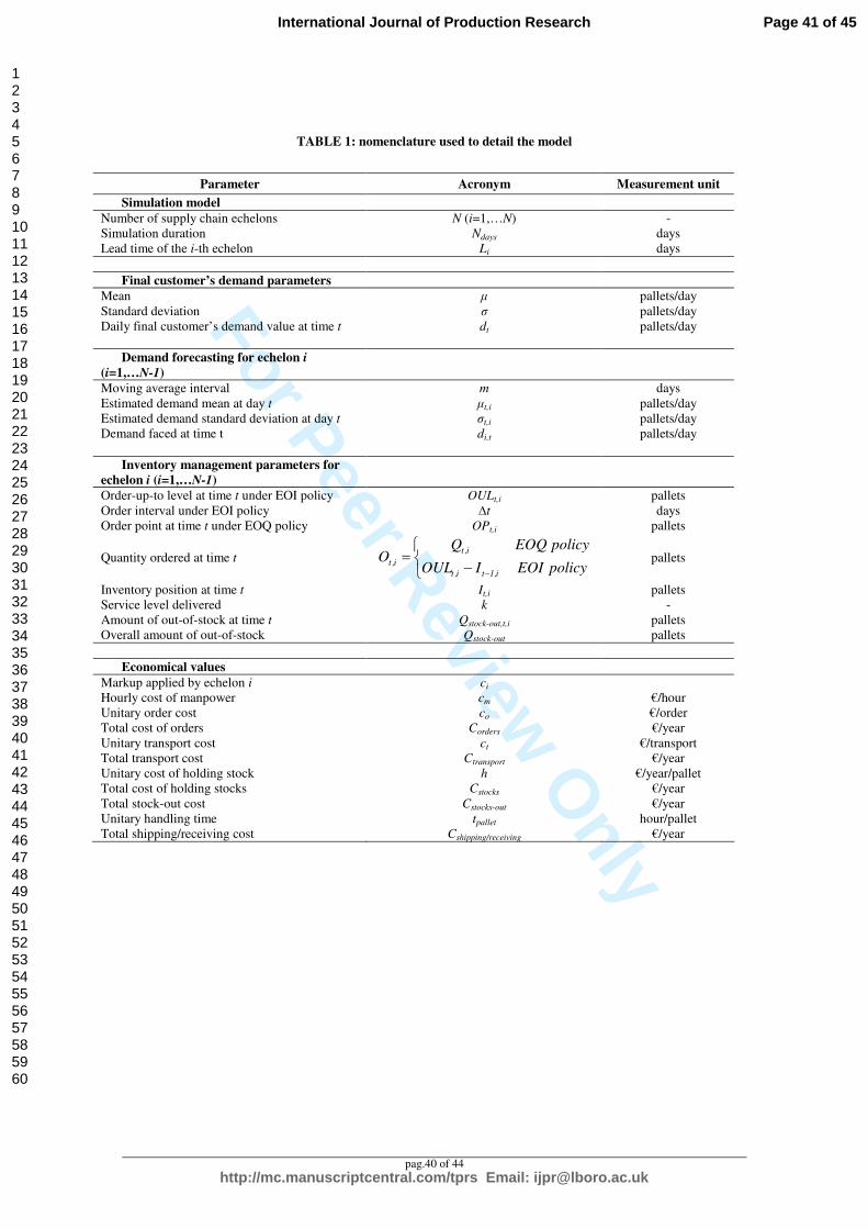
Thinking International Inc.). The nomenclature proposed in TABLE 1 is used to describe the

model and the corresponding input parameters.

INSERT TABLE 1

In this study, we adopt the representation by Shapiro (2001), suggesting that the supply chain

can be described in terms of two main processes, namely products flow and orders flow.

Accordingly, the generic i-th echelon (i=1,..N) receives orders from echelon i-1 and products

(i.e. pallets) from echelon i+1, through transport activities. For each echelon, a procurement

lead time Li is introduced, encompassing the time required for transports, ordering and

warehousing activities. We assume deterministic lead time (Dejonckheere et al., 2003), and thus

order crossover phenomena (Reizebos, 2006) are not considered in this study. For simplicity,

we model the flow of a single product.

According to several studies in literature (Chatfield et al., 2004; Zhang, 2004), the number of

players per echelon is set at one. Echelon 1 (i.e., the retail store) directly faces the final

customer’s demand, whose value at day t is dt. Customer’s demand is a stochastic variable, with

normal distribution N(µ;σ). Other supply chain players (except the manufacturer) forecast

demand through a moving average model based on the last m observations (Chen et al., 2000;

Zhang, 2004; Sun & Ren, 2005).

Each player stores product in a warehouse, whose inventory level is initially set at a defined

value. This latter is assumed to be the same for all echelons considered, except echelon N, for

which an infinite stock availability is hypothesised.

Page 7 of 45



123456789101112131415161718192021222324252627282930313233343536373839404142434445464748495051525354555657585960

For Peer Review O

nly

7

3.2 The supply chain configurations considered

In this section, we describe the supply chain configurations examined in this study, in terms of

the following parameters: (i) number of players; (ii) reorder policy; (iii) demand information

sharing mechanisms; and (iv) demand behaviour.

3.2.1 Number of echelons

The supply chain modelled may range from 3 (i.e. manufacturer – distributor – retail store) up

to 5 echelons (i.e. manufacturer – distributor1 – distributor2 – distributor3 - retail store).

3.2.2 Reorder policy

Each player can place orders according to an Economic Order Quantity (EOQ) or Economic

Order Interval (EOI) policy. The same reorder policy is assumed for all supply chain players.

Under EOI policy, the reorder process of echelon i can be described as follows:

i. at time t (t=1,...Ndays), the i-th echelon estimates demand mean (µt,i) and standard

deviation (σt,i) according to the moving average model, i.e.:

( )∑

∑

−=

−=

−−

=

=

t

mtk

2

i,ti,k

2

i,t

t

mtk

i,ki,t

d1m

1

dm

1

µσ

µ

(1)

where dt,i indicates the demand faced by echelon i at time t, corresponding either to the

final customer’s demand or to orders placed by echelon i-1, i.e.:

−=

==

− 1,...2

1

1,

,NiO

idd

it

t

it (2)

ii. the above values are used to compute the order-up-to level at time t (OULt,i), according

to eq.3 (Bottani et al., 2007; Dejonckheere et al., 2003):

2

,,, )()( itiitiit LtkLtOUL σµ +∆++∆= (3)

Page 8 of 45



123456789101112131415161718192021222324252627282930313233343536373839404142434445464748495051525354555657585960

For Peer Review O

nly

8

iii. each ∆t, the supply chain player checks the stock available It-1,i to decide whether to

place an order. The amount of product to be ordered is derived as OULt,i-It-1,i. It should

be noted that It-1,i also takes into account products ordered but not yet received;

iv. whenever the order is placed, the inventory level It,i is updated based on OULt,i.

Under EOQ policy, the reorder process of echelon i is as follows:

i. eq.1 is exploited to estimate µt,i and σt,i at time t;

ii. the above parameters are used to compute the value of OPt,i, based on eq.4 (Bottani et

al., 2007; Dejonckheere et al., 2003):

2

,,, itiitiit LkLOP σµ += (4)

iii. in the case It-1,i<OPt,i, the supply chain player places an order. The quantity to be

ordered Qt,i is computed starting from µt,i, as detailed below:

h

c2Q oi,t

i,t

××=

µ (5)

iv. at time t, the inventory level It,i of echelon i is updated based on the observed demand

dt,i, i.e.

itititit QdII ,,,1, +−= − (6)

As we modelled a stochastic demand, orders placed by supply chain players could always

exceed the available product stock, resulting in a stock-out. Under such circumstance, orders are

fulfilled by an external supplier, with infinite products availability. The overall quantity

supplied by this player (Qstock-out) is used to assess the corresponding stock-out costs. In the case

the stock-out occurs at the retail store, it is assumed that the final customer buys the quantity of

products available; conversely, for all the remaining players, Qstock-out,i accounts for the whole

quantity ordered to echelon i. Eq.7 summarises the computation of Qstock-out,i:

Page 9 of 45



123456789101112131415161718192021222324252627282930313233343536373839404142434445464748495051525354555657585960

For Peer Review O

nly

9

−=

=−=

−

−−− 1,...2

1

1,

1,1

,,NiO

iIdQ

it

itt

itoutstock (7)

Due to infinite stock availability, no stock-out may occur for the manufacturer.

3.2.3 Information sharing mechanisms

Point of sale (POS) data can be shared between supply chain players or only available to the

retail store. Under this latter scenario, echelon i forecasts demand only based on dt,i previously

defined in eq.2. Conversely, when POS data are shared, this additional information is available

to all supply chain players to forecast demand. Hence, for i=1,…N-1 we have dt,i=dt in eq.2.

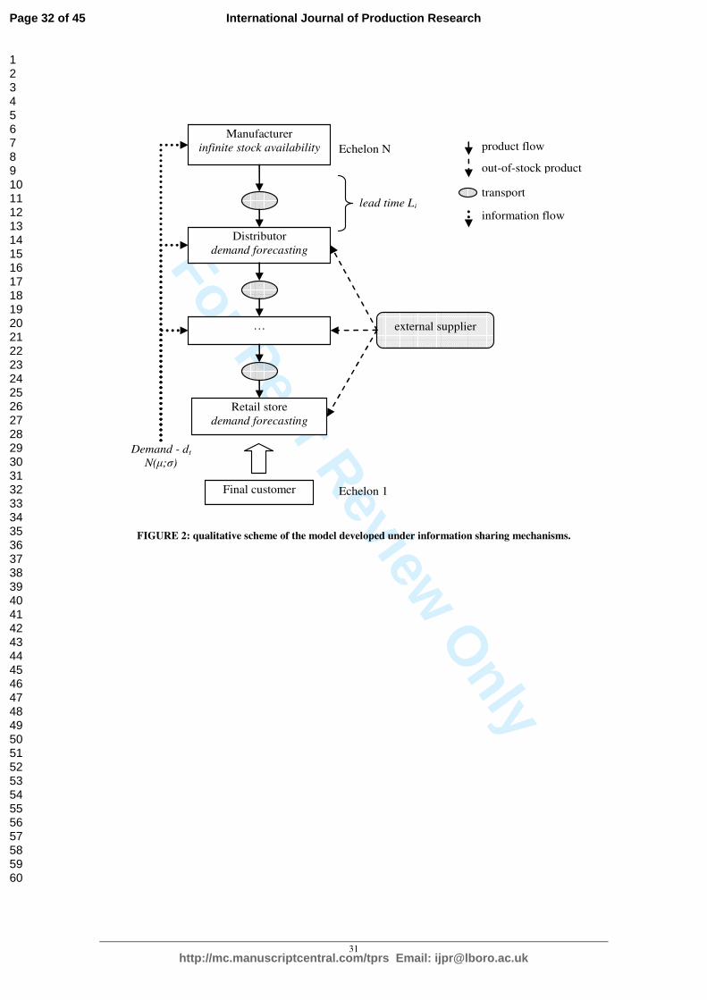
FIGURE 1 and FIGURE 2 show a scheme of the model structure (in terms of products, orders

and information flow) respectively under absence of information sharing and when information

sharing mechanisms are implemented.

INSERT FIGURE 1 AND FIGURE 2

Demand information sharing can be seen as a possible consequence of the adoption of advanced

Information Technology (IT) tools for product identification and monitoring. This is, for

instance, the case of Radio Frequency Identification (RFID) coupled with EPC Network

(Bottani & Rizzi, 2008).

3.2.4 Demand behaviour

The final customer’s demand may or may not experience an increase, referred to as demand

“peak”, during a simulation run. In the case of non-increase, the demand mean and standard

deviation are known parameters (µ and σ). When simulating an increase in demand, the demand

mean and standard deviation are changed to µ’=2µ and σ’=σ at the middle of the simulation,

and kept unchanged until the simulation ends.

Under the EOQ policy, the “peak” of demand involves updating Qt,i and OPt,i parameters, by

exploiting eqs.4-5 with µ’ and σ’. The same happens, under EOI policy, for the OULt,i parameter

Page 10 of 45



123456789101112131415161718192021222324252627282930313233343536373839404142434445464748495051525354555657585960

For Peer Review O

nly

10

(eq.3). Moreover, the reorder interval ∆t also depends on the demand mean; in this regard, in

real cases, it is expected that each supply chain echelon will modify ∆t based on µ’ and σ’. In

modelling this behaviour, we consider two additional scenarios, namely:

a. “responsive” supply chain players (Lowson et al., 1999) – ∆t is updated 3 days

after the demand “peak” occurred;

b. “non-responsive” supply chain players - ∆t is updated 5 days after the demand

“peak” occurred.

3.3 Experiments setting and outcomes

To provide a detailed investigation of the supply chain, we examine 30 different scenarios,

which are obtained by combining the parameters described in the above sections, according to

Design of Experiments (DoE) (Montgomery & Runger, 2003). The resulting scheme is

proposed in FIGURE 3.

INSERT FIGURE 3

For each scenario, we assessed the outputs listed below (numerical values of input parameters

required for the computation are detailed in section 3.4):

i. Bullwhip effect, defined as the ratio between variance of orders received by echelon N

and the variance of final customer’s demand, i.e. . Under “peak” of demand, the

resulting σ is analytically computed based on dt values;

ii. cost of holding stocks (Cstocks): it is computed starting from unitary cost of stocks and

amount of stock available at the warehouse, i.e.:

(8)

Page 11 of 45



123456789101112131415161718192021222324252627282930313233343536373839404142434445464748495051525354555657585960

For Peer Review O

nly

11

Due to infinite stock availability, such cost is not computed for the manufacturer;

iii. stock-out cost (Cstock-out): it is computed starting from the mark-up applied by each

supply chain player (ci), corresponding to the economical loss experienced, and from

Qstock-out,t,i, as described by eq.9:

(9)

iv. order cost (Corder): it results from unitary cost of orders co and number of orders placed

by supply chain players Norders,i (except the manufacturer), i.e.:

(10)

The number of orders is a direct outcome of the simulation run;

v. transport cost (Ctransport): transport cost is assumed not to be affected by the order

quantity, and to only depend upon the number of orders fulfilled. It thus results from

Norders,i and unitary cost of transport (ct), according to eq.11:

(11)

vi. shipping/receiving cost (Cshipping/receiving): for each echelon, this cost is derived from

average number of pallets handled per year, average hourly cost of manpower (cm) and

time required to handle a pallet (tpallet). As the model considers a player per echelon, the

average number of pallets handled reflects the average customer’s demand (µ), which is

the same for all echelons. Hence, Cshipping/receiving only depends on the number of echelons

considered. In the computation, it should also be considered that the manufacturer only

performs shipping activities, while the retail store only performs receiving activities.

The following formula is thus used to assess Cshipping/receiving:

Page 12 of 45



123456789101112131415161718192021222324252627282930313233343536373839404142434445464748495051525354555657585960

For Peer Review O

nly

12

(12)

3.4 Input data

Input data used in the model were derived from a previous study in the field of the FMCG

supply chain, performed by one of the authors. Some details concerning the data collected in the

previous work and the case study features are proposed in Appendix. The reader is referred to

Bottani & Rizzi, (2008), for a comprehensive description of the case study.

The data used for the present study are described in the following list.

• The initial value of the inventory level is set at 472 pallets for echelons 1,…N-1. Such

value is derived from the average capacity of a FMCG warehouse (i.e., 500 pallets),

which is usually at 80% saturation;

• the demand distribution is characterized by µ=150 pallets/day and σ=42 pallets/day.

Those values are used under absence of demand “peak”; when “peak” of demand

occurs, they are updated to µ’=300 pallets/day and σ’=59.4 pallets/day;

• the service level provided by supply chain players, corresponding to the probability to

fulfil orders with the available stock, is set at 90%. Consequently, we have k=1.28 in

eqs.3-4;

• the moving average interval is m=5 for distributors and m=6 for the retail store;

• Li is set at 4.5 days for all supply chain players, except the manufacturer, whose lead

time is 10 days. In both cases, 0.5 days are spent for transport activities;

• h is estimated in approx 153.52 €/pallet/year, corresponding to 0.42 €/pallet/day, which

is derived as the average between costs experienced by distributor and manufacturer;

• the average value of products in the FMCG context accounts for 475 €/pallet. It is

supposed that each echelon applies 10% mark-up to this value, which is close to typical

Page 13 of 45



123456789101112131415161718192021222324252627282930313233343536373839404142434445464748495051525354555657585960

For Peer Review O

nly

13

mark-up for food products (Anderson & Billou, 2007). Hence, ci in eq.9 varies

depending on the echelon considered;

• co and ct are set at 10 €/order and 780 €/transport, respectively;

• Cshipping/receiving is estimated in approx 123,187.50 €/year/echelon under absence of

demand “peak” and for 185,287.50 €/year/echelon when demand “peak” is considered;

• ∆t, computed starting from the parameters described above, accounts for 5 days under

absence of demand “peak”, and is changed to 3 days when demand “peak” is observed.

4 Results and discussion

The simulation duration was set at Ndays=365 days. For each scenario, 25 replications were

performed. This value was observed to allow reaching stabilization of the simulation outputs for

echelon N. As an example of stabilization of model outputs, FIGURE 4 shows the number of

orders received by echelon N under “EOQ-5-no_sharing-no_peak” scenario as a function of the

number of replications.

INSERT FIGURE 4

Bullwhip effect results are detailed in TABLE 2, and graphically illustrated in FIGURE 5, in

terms of standard deviation ratio (σN/σ), instead of variance ratio, to simplify the representation.

TABLE 3 and FIGURE 6 provide a detailed illustration of the costs resulting in the scenarios

examined. Statistical analysis of outcomes was also performed, with the aim to identify and

assess single and combined effects of the supply chain parameters on the simulation results. The

procedure described by Montgomery & Runger, (2003), was followed to this extent. Outcomes,

in terms of Sum of Squares (SS), Mean Square (MS), F-test and corresponding significance

value (sig.) are proposed in TABLE 4. It should be noted that this analysis is limited to 20

scenarios, resulting from the following combinations of factors:

• reorder policy (factor A) – EOQ (low) or EOI (high);

Page 14 of 45



123456789101112131415161718192021222324252627282930313233343536373839404142434445464748495051525354555657585960

For Peer Review O

nly

14

• number of supply chain echelons (factor B) – 3 (low) or 5 (high);

• demand information sharing (factor C) – absence (low) or presence (high) of

information sharing mechanisms;

• demand behaviour (factor D) – absence (low) or presence (high) of demand “peak”;

• responsiveness (factor E) – non responsive (low) or responsive (high) supply chain

players. This factor is only considered in conjunction with demand peak (D) under EOI

(A) inventory management policy, according to the previous description.

FIGURE 7÷FIGURE 10 join the total costs with the bullwhip effect results; outcomes are

shared into four quadrants, resulting from the combination of high/low values of total

costs/bullwhip effect1. Dots in FIGURE 7÷FIGURE 10 represent the scenarios examined; the

corresponding percentage values of total cost and bullwhip effect are proposed in TABLE 5. For

each quadrant, the percentage sharing of number of supply chain players (FIGURE 7), inventory

management policies (FIGURE 8), information sharing mechanisms (FIGURE 9) and demand

behaviour (FIGURE 10) is displayed.

INSERT TABLE 2÷TABLE 5 and FIGURE 5÷FIGURE 10

4.1 Bullwhip effect results

To validate the model outcomes, the bullwhip effect values from the simulation runs were

compared with those resulting from the application of the analytical approach by Chen et al.,

(2000). Specifically, the authors derived a lower bound for the variance amplification for

echelon i, expressed as:

2

2

11

2

222

1)(

)(

m

L

m

L

d

o

i

k

k

i

k

k

i

+

+≥∑∑==

σσ

(13)

1 For visualization purpose, boundaries to the high/low values of both costs and bullwhip effect were set at 12.5% of the maximum

observed value.

Page 15 of 45



123456789101112131415161718192021222324252627282930313233343536373839404142434445464748495051525354555657585960

For Peer Review O

nly

15

being σ2(oi) the variance of orders placed by the i-th supply chain echelon, σ

2(d) the variance of

the final customer’s demand, Li the procurement lead time of echelon i, and m the moving

average interval. As the above formula is valid under demand information sharing and EOQ

inventory management policy, we compare analytical results with simulation outcomes for the

“EOQ-5-sharing-no_peak” scenario. It should be noted that in eq.13 the same value of m is

assumed for all echelons, which is not the case considered in our study. Hence, two

computations were performed with m=5 and m=6, obtaining σ2

N/σ2=54.58 and σ

2N/σ

2=39.51,

respectively. It can be seen from TABLE 2 that the simulated bullwhip effect for this scenario

correctly results in an intermediate value, i.e. 46.11, providing validation of the model

developed.

Bullwhip effect outcomes can be summarised in the following key results.

Result 1: other things being equal, the bullwhip effect in higher under EOI than under EOQ

inventory management policy.

This result was expected; in fact, under an EOI policy, orders are placed at a defined time

interval ∆t, while the quantity ordered is null in other periods. As a result, an amplification of

the demand variance is observed by the supplier. This confirms a similar result by Jakšič &

Rusjan, (2008), which observed that “order-up-to” replenishment rules induce higher bullwhip

effect than others inventory management policies. Outcomes from TABLE 4 also show that the

impact of factor A on the resulting bullwhip effect is statistically significant at p<0.05.

Result 2: other things being equal, the bullwhip effect is greater when the number of supply

chain players increase.

Again, this result was expected, as it is a direct consequence of the bullwhip effect definition

(see eq.13). As can be seen from TABLE 4, statistical analyses show a significant (p<0.05)

Page 16 of 45



123456789101112131415161718192021222324252627282930313233343536373839404142434445464748495051525354555657585960

For Peer Review O

nly

16

impact of number of factor B on the resulting bullwhip effect. FIGURE 7 shows that supply

chains with high bullwhip effect and high total costs encompass 4 (43%) or 5 (57%) echelons,

while supply chains with high bullwhip effect and low total costs are composed of 3 (50%) or 4

(50%) echelons.

From TABLE 2 it can also be noted that the number of supply chain players substantially

increase the bullwhip effect under absence of information sharing; conversely, under

information sharing, outcomes of the simulation runs support this result to a lower extent. In this

regard, focusing on TABLE 4, it can be appreciated that the combined effect of demand

information sharing and number of supply chain players (i.e. factors BC) has not significant

impact on the bullwhip effect. This could be explained considering that complete supply chain

visibility provides, as output, substantially lower demand amplification; consequently, most of

the resulting scenarios are characterised by similar values of the bullwhip effect, regardless of

the number of echelons.

Outcomes of TABLE 4 also suggest that the combined implementation of EOI inventory

management policy and high number of supply chain echelons (i.e., factors AB) has a

significant (p<0.05) impact on the resulting bullwhip effect. As explained in result 1, under an

EOI policy, several “null” orders are observed, as supply chain players place orders every ∆t. In

particular, as the OULt,i is computed according to the orders received (see eqs.1 and 3), under

this scenario it is found that, due to substantial demand variance amplification, orders to echelon

N are very limited in number. Conversely, quantities ordered are dramatically increased. This

effect is particularly evident for high N.

Result 3: other things being equal, the bullwhip effect is greater under absence of information

sharing.

Page 17 of 45



123456789101112131415161718192021222324252627282930313233343536373839404142434445464748495051525354555657585960

For Peer Review O

nly

17

This result is known in literature (Lee et al., 2000; Chen et al., 2004; Chatfield et al., 2004), and

should be ascribed to the possibility of supply chain players to exploit POS data, rather than

orders, to forecast demand, thus reducing the resulting variability. Statistical analyses also show

that demand information sharing is the factor having the highest impact on the bullwhip effect

(p=0.002). FIGURE 9 also shows that 100% of scenarios experiencing high bullwhip effect are

characterised by absence of information sharing mechanisms.

Interestingly, a statistically significant impact of demand information sharing mechanisms in

conjunction with EOI policy, with/without high number of supply chain echelons (i.e., factors

BC/factors ABC) on the resulting bullwhip effect can be observed from the results obtained.

Result 4: under some circumstances, the bullwhip effect is lower when a “peak” of demand is

introduced in the supply chain.

Outcomes from TABLE 4 show that the single effect of the “peak” of demand against the

bullwhip effect is not statistically significant (p>0.05); this suggests that the demand “peak”, per

se, does not significantly affect the observed bullwhip effect. In this regard, it can be seen from

FIGURE 10 that high bullwhip effect may occur either under presence or absence of demand

“peak”. From the same figure, it is also interesting to note that high bullwhip effect combined

with low total cost always occur under absence of demand “peak” (100% of the scenarios

examined).

The combined introduction of demand “peak” and EOI inventory management policy (i.e.,

factors AD), as well as of demand “peak” and high number of supply chain players (i.e., factors

BD), have significant impact on the resulting bullwhip effect. Specifically, outcomes in TABLE

2 indicate that a lower bullwhip effect is usually observed when demand “peak” is introduced in

the model. The same result is indicated in FIGURE 8, which shows that scenarios with high

bullwhip effect and high total costs are mainly characterised by EOI policy (86% of the

Page 18 of 45



123456789101112131415161718192021222324252627282930313233343536373839404142434445464748495051525354555657585960

For Peer Review O

nly

18

scenarios examined), while EOI and EOQ policies are equally shared in scenarios with high

bullwhip effect and low total costs.

From an operational perspective, this result could be explained considering that, when an

unexpected increase in demand is observed, a supply chain player tends to increase the number

of orders placed. Under an EOI policy, this involves reducing the ordering interval ∆t;

consequently, a lower number of “null” orders are observed. From the computational point of

view, a lower order variance emerges. This effect is particularly emphasised when N=5, as can

be seen from FIGURE 7.

Result 5: under “peak” of demand, the bullwhip effect is lower if the supply chain is able to

quickly react to the demand variation.

This result is evident from numerical outcomes in TABLE 2, as all “responsive” scenarios show

a lower bullwhip effect than the corresponding “non responsive” ones. A reactive supply chain

player is able to quickly update the reorder policy parameters (i.e., the order interval ∆t), which

results in the capability to better follow the demand trend, avoiding to introduce additional

variability. Nonetheless, it should be noted that no statistical evidence can be provided in this

regard.

4.2 Costs analysis

Outcomes from cost analysis can be summarized in the following key points.

Result 6: the total costs observed under scenarios “EOI-5-no_sharing-peak-no_resp”, “EOI-5-

no_sharing-no_peak”, and “EOI-5-no_sharing-peak-resp” are significantly higher than all the

remaining scenarios.

Page 19 of 45



123456789101112131415161718192021222324252627282930313233343536373839404142434445464748495051525354555657585960

For Peer Review O

nly

19

This result was derived from the analysis of outcomes in TABLE 3. The above scenarios are all

composed of 5 echelons, and operate under EOI policy and absence of information sharing. The

resulting costs ranges from about 15 to 19 million €/year, while all other scenarios experience

costs lower than 7 million €/year. It can be easily noted that the costs are almost entirely due to

stocks, which account for 83.2% (under “EOI-5-no_sharing-peak-resp” scenario) to 86.8%

(under “EOI-5-no_sharing-peak-no_resp” scenario) of the total costs. This result, in turn, is a

consequence of the bullwhip effect observed, ranging from 53.24 to 108.4 in terms of σN/σ for

the scenarios considered (see TABLE 2), which involves high safety stock levels. In particular,

looking at FIGURE 8 and FIGURE 9, one can see that high bullwhip effect combined with high

total costs is mainly observed under EOI policy (86% of the scenarios examined) and absence of

information sharing mechanisms (100% of the scenarios examined).

Result 7: other things being equal, the total costs observed are significantly higher when the

number of supply chain players increase.

The number of supply chain echelons has the highest impact on the observed total costs of the

supply chain (p=0.000). In particular, statistically significant effects of factor B are observed

against all cost components considered in this study. FIGURE 7 confirms that supply chain

configurations with high costs are only composed of 4 or 5 echelons.

This is an obvious result, since the increase in the number of supply chain echelons clearly

involves increase in all cost components considered, due to the need of adding the cost

contributions of each echelon (see eqs.8-12).

Result 8: other things being equal, the total costs observed are significantly higher under EOI

than EOQ inventory management policy.

Page 20 of 45



123456789101112131415161718192021222324252627282930313233343536373839404142434445464748495051525354555657585960

For Peer Review O

nly

20

This result, which is supported from previous studies by Chopra & Meindl, (2004), can be

observed from outcomes in TABLE 4, indicating a high significance of factor A on the resulting

total costs (p<0.05). Overall, statistical analyses indicate that factor A substantially affects most

of the costs components examined, except stock-out costs, and that its impact is statistically

significant at p<0.05. In this regard, FIGURE 8 highlights that high costs coupled by high

bullwhip effect are mainly observed under EOI rather than EOQ policy (86% vs. 14% of the

scenarios examined), while EOI and EOQ are equally shared in scenarios experiencing high cost

with low bullwhip effect.

As mentioned already, EOI policy usually involves a higher average stock level, as a

consequence of the lower number of orders, with wider quantities. This is confirmed by

statistical analyses performed, which highlight a significant impact (p=0.002) of factor A on the

resulting costs of holding stocks. As order and transport costs are both computed starting from

the number of orders (see eqs.11-12), the statistically significant impact of EOI inventory

management policy on those cost components is a direct consequence of the number of orders

placed by supply chain players under that policy.

As a further outcome, the combined effect of factors AB (i.e., EOI policy coupled with high

number of supply chain echelons) is also found to significantly impact the total costs.

Specifically, it is reasonable that factors AB substantially increase each cost component

examined, since both the number of echelons and the EOI policy involve a significant increase

of the cost components. This is confirmed by results in TABLE 3.

Result 9: other things being equal, the total costs observed tend to be lower when demand

information sharing is introduced. However, demand information sharing has a different impact

on each cost component.

Page 21 of 45



123456789101112131415161718192021222324252627282930313233343536373839404142434445464748495051525354555657585960

For Peer Review O

nly

21

From TABLE 3, TABLE 4 and FIGURE 9, it can be appreciated that total costs observed are

usually lower when demand information sharing mechanisms are introduced, and that the effect

is statistically significant at p=0.001.

This result is a consequence of several effects. As a first point, it can be observed from TABLE

3 that costs of holding stocks are substantially lower under demand information sharing. In fact,

as mentioned in result 3, the availability of POS data allows reducing the orders variability,

resulting in a lower bullwhip effect and in a significant reduction of the amount of stocks

required at each supply chain echelon. In this regard, a significant impact (p=0.000) of demand

information sharing mechanisms on the resulting costs of holding stocks is observed in TABLE

4. Although this is a general result, it can be particularly appreciated when examining a 5-

echelon supply chain, where the resulting bullwhip effect is extremely high (see TABLE 2 and

result 2).

Conversely, results presented in TABLE 3 indicate that stock-out costs tend to increase when

demand information sharing is implemented, although the availability of POS data, per se, has

no significant effect (p=0.055) on the observed stock-out costs. This result should mainly be

ascribed to the way stock-out costs were modelled in our study. In fact, under demand

information sharing, each supply chain player places orders based on POS data; hence,

quantities ordered are usually lower than those required under unknown customer’s demand,

resulting in reduced average stock level. However, under stochastic demand it is always

possible that demand values (and consequently orders placed) exceed the amount of stocks

available; this is exacerbated when the average stock level is lower. Consequently, stock-out

costs increase under demand information sharing mechanism.

Finally, demand information sharing mechanisms appear to significantly affect the observed

order (p=0.003) and transport (p=0.003) costs. Looking at TABLE 3, it can be seen that, in

particular, demand information sharing tends to increase the resulting order and transport costs.

In fact, the availability of POS data allows reducing the observed demand variability, allowing

Page 22 of 45



123456789101112131415161718192021222324252627282930313233343536373839404142434445464748495051525354555657585960

For Peer Review O

nly

22

orders placed to better follow the demand behaviour: specifically, lower quantities are ordered

more frequently, with a resulting increase in the number of orders placed.

The combined effect of the above described cost components leads to very different results,

depending on the supply chain configuration examined. More precisely, it can be seen from

FIGURE 6 and TABLE 3 that costs of holding stocks are by far the most important cost

component of 5-echelon supply chains. Demand information sharing thus involves a significant

decrease of costs for those supply chains. An opposite situation occurs for 3-echelon supply

chains. In fact, given the low number of echelons, this supply chain configuration is affected by

costs of holding stocks and stock-out costs to a similar extent: such costs account for about 35%

and 37% on the total costs, respectively. By amplifying the stock-out costs, information sharing

leads to a slight increase of the total costs for those scenarios. Finally, 4-echelon supply chain

scenarios appear to be closer to 5-echelon ones, i.e. information sharing involves decrease in the

total costs; however, due to the lower number of echelons, this result is less evident.

Besides the above result, outcomes of the statistical analysis and economical assessment also

show that demand information sharing mechanisms, in conjunction with EOI policy and high

number of supply chain echelons (i.e. factors ABC), appear to significantly affect the observed

order (p=0.005) and transport (p=0.007) costs, and in particular tend to increase such costs. This

is again a consequence of the increased number of orders placed, resulting from the reduced

demand variability and corresponding decrease of quantities per order.

Result 10: other things being equal, the total costs observed increase when “peak” of demand is

introduced.

Results in TABLE 3, TABLE 4 and FIGURE 10 indicate that total supply chain costs are higher

when “peak” of demand is introduced, and that the impact of demand “peak” (i.e., factor D) on

the observed costs is significant at p=0.012. More precisely, demand “peak” involves increase

Page 23 of 45



123456789101112131415161718192021222324252627282930313233343536373839404142434445464748495051525354555657585960

For Peer Review O

nly

23

of stock-out (p=0.005), order (p=0.000), transport (p=0.000), and shipping/receiving (p=0.000)

costs, resulting in substantially higher total costs.

The increase of stock-out costs was expected, since, as a consequence of demand “peak”, the

amount of stock available for each supply chain player is more likely to be lower than the

quantity requested. Moreover, as already discussed, when a demand increase is introduced, a

supply chain player tends to increase the number of orders placed, regardless of the inventory

management policy applied. Hence, an increase in order costs and corresponding transport costs

is observed. Finally, due to the computational procedure followed, shipping/receiving costs are

amplified as a consequence of the increased quantity of pallets handled per year.

The combined effect of factors AD (i.e., demand peak and EOI inventory management policy)

on the total costs, and in particular on the costs of holding stocks, is also significant. It can be

observed from TABLE 3 that cost of holding stocks tends to increase under peak of demand and

EOI policy. This result should be ascribed to the increased order variance caused by demand

peak under EOI inventory management policy, which, in turn, involves increase in the required

safety stocks for each echelon.

Similar considerations can be drawn for the combined effect of factors BD (i.e., demand “peak”

coupled with high number of supply chain echelons) on the total costs. More precisely, factors

BD significantly affect the resulting costs of holding stocks (p=0.000), orders (p=0.031) and

transport (p=0.036). From TABLE 3, it can be seen that all the above costs components tend to

be higher when examining 5-echelon supply chains under demand “peak”. As previously

mentioned, the higher order variance caused by demand “peak” involves increase in the required

safety stocks for each supply chain echelon, resulting in a corresponding increase in their costs.

Demand “peak” also involves an increase in the number of orders placed, due to higher demand

observed. Order and transport costs are thus amplified correspondingly.

Page 24 of 45



123456789101112131415161718192021222324252627282930313233343536373839404142434445464748495051525354555657585960

For Peer Review O

nly

24

Result 11: other things being equal, under “peak” of demand, the total costs observed decrease

if the supply chain is able to quickly react to the demand variation.

It can be seen from TABLE 4 that the combined effect of demand “peak” and responsiveness,

under EOI inventory management policy (i.e., factors ADE) has a significant impact (p=0.03)

on the resulting total costs observed. In fact, a quick reaction of the supply chain implies that

each player updates inventory management parameters (in particular, the ∆t interval)

immediately after the demand “peak” is observed. The main outcome of such reaction is that the

average stock level is quickly adapted to the new demand value, thus optimizing the overall cost

of stocks. Outcomes from TABLE 4 also highlight that the combined effect of factors ADE

significantly decreases the resulting stock-out (p=0.034), order (p=0.000), transport (p=0.000)

and shipping/receiving (p=0.001) costs. As a result, the observed total costs decrease under this

scenario.

5 Conclusions

Based on a discrete-event simulation model, reproducing a Fast Moving Consumer Goods

(FMCG) supply chain, we have provided a quantitative assessment of the effects of different

configurations on the total costs and bullwhip effect observed in the supply chain. Our analysis

covers 30 possible supply chain configurations, resulting from the combination of several

design parameters, such as number of echelons, reorder policy adopted, demand information

sharing mechanisms, demand behaviour, and responsiveness. For each scenario, total costs and

bullwhip effect were computed starting from simulation outcomes and several input parameters

available in literature. Moreover, a statistical analysis of effects was performed to identify

possible significant impact of single/combined supply chain design parameters on the resulting

costs and demand variance amplification.

The key results of this study show that both the total logistics cost and the bullwhip effect are

affected by all supply chain design parameters examined, although to a different extent. In

Page 25 of 45



123456789101112131415161718192021222324252627282930313233343536373839404142434445464748495051525354555657585960

For Peer Review O

nly

25

particular, the number of supply chain echelons and the implementation of an EOI inventory

management policy involve a substantial increase in the total costs and bullwhip effect, and

their impact is significant at p<0.05. The presence of demand “peak” also causes an increase in

the total logistics costs, although, per se, it does not significantly affect the resulting bullwhip

effect. Conversely, demand information sharing mechanisms tend to reduce both the bullwhip

effect and the resulting total costs, due to the significant (p=0.000) decrease in costs of holding

stocks.

As the simulation model was developed using average data of the FMCG context, our results

can be useful in practice to identify the optimal supply chain configuration as a function of the

operating conditions. Moreover, outcomes from this study provide some insights about the

supply chain cost components and their trend depending on the configuration considered.

Our study is grounded on the simulation of a single-product flow. To derive more general

results, it would be appropriate to extend the model to include: (1) the flow of different

products, with different characteristics; (2) several supply chain players per echelon; (3) lead-

time stochasticity and corresponding order crossover investigation; and (4) a sensitivity analysis

of model outcomes as a function of different values of the input parameters.

References

Anderson, J. and Billou, N., 2007. Serving the world’s poor: innovation at the base of the economic pyramid, Journal

of Business Strategy, 28(2), 14-21

Bottani, E. and Rizzi, A., 2008. Economical assessment of the impact of RFID technology and EPC system on the

Fast Moving Consumer Goods supply chain. International Journal of Production Economics, 112(2), 548-569

Bottani, E., Montanari, R. and Volpi, A., 2007. Quantifying the Bullwhip Effect in inventory management policies.

Proceedings of the 12th International Symposium in Logistics, Budapest (Hungary)

Bowersox, J., and Closs, D.J., 1996. Logistical management. McGraw-Hill, New York

Chan, F.T.S. and Chan, H.K., 2005. Simulation modeling for comparative evaluation of supply chain management

strategies. Journal of Advanced Manufacturing Technology, 25, 998–1006.

Page 26 of 45



123456789101112131415161718192021222324252627282930313233343536373839404142434445464748495051525354555657585960

For Peer Review O

nly

26

Chatfield, D.C., Kim, J.G., Harrison, T. P. and Hayya, J.C., 2004. The Bullwhip Effect—Impact of Stochastic Lead

Time, Information Quality, and Information Sharing: A Simulation Study. Production and Operations Management

13(4), 340-353

Chen, F., Drezner, Z., Ryan, J.K. and Simchi-Levi, D., 2000. Quantifying the bullwhip effect in a simple supply

chain: the impact of forecasting, lead time, and information. Management Science 46(3), 436-443

Chopra, S. and Meindl, P., 2004. Supply chain management: Strategy, planning and operations (2nd edition). Prentice

Hall, Upper Saddle River, NJ

Cooper, M.C., Lambert, D.M. and Pagh, J.D., 1997. Supply chain management: More than a new name for logistics.

The International Journal of Logistics Management, 8(1), 1–13

Dejonckheere, J., Disney, S.M., Lambrecht, M.R. and Towill, D.R., 2003. Measuring and avoiding the bullwhip

effect: A control theoretic approach. European Journal of Operational Research 147, 567–590

Hammami, R., Frein, Y. and Hadj-Alouane, A.B., 2008. Supply chain design in the delocalization context: Relevant

features and new modeling tendencies. International Journal of Production Economics, 113(2), 641-656

Harrison J.R., Lin Z., Carroll G.R. and Carley K.M., 2007. Simulation modeling in organizational and management

research. Academy of Management Review, 32(4), 1229–1245

Higuchi, T. and Troutt, M.D., 2004. Dynamic simulation of the supply chain for a short life cycle product—Lessons

from the Tamagotchi case. Computers & Operations Research, 31, 1097–1114

Hwarng, H.B., Chong, C.S.P., Xie, N. and Burgess, T.F., 2005. Modelling a complex supply chain: understanding the

effect of simplified assumptions. International Journal of Production Research, 43(13), 2829–2872

Iannone, R., Miranda, S. and Riemma, S., 2007. Supply chain distributed simulation: An efficient architecture for

multi-model synchronization. Simulation Modelling Practice and Theory, 15, 221–236

Jakšič, M., and Rusjan, B., 2008. The effect of replenishment policies on the bullwhip effect: A transfer function

approach. European Journal of Operational Research, 184, 946–961

Lambert, D.M., 2001. The supply chain management and logistics controversy. In Brewer, A., Button, K.J., Hensher,

D.A., (Eds.), Handbook of Logistics and Supply Chain Management. Pergamon, Oxford

Lau, J.S.K., Huang, G.Q. and Mak, K.L., 2004. Impact of information sharing on inventory replenishment in

divergent supply chains. International Journal of Production Research 42(5), 919–941

Lee, H.L., Padmanabhan, V., and Whang, S., 2004. Information distortion in the supply chain: the bullwhip effect.

Management Science 50(12), 1875-1886

Lee, H.L., So K.C., and Tang, C.S., 2000. The value of information sharing in a two-level supply chain. Management

Science, 46(5), 626-643

Lowson, B., King, R., and Hunter, A., 1999. Quick Response: Managing the Supply Chain to Meet Customer

Demand. John Wiley & Sons, Chichester

Longo, F., and Mirabelli, G., 2008. An advanced supply chain management tool based on modeling and simulation.

Computers & Industrial Engineering, 54, 570–588

Montgomery, D.C., and Runger G.C., 2003. Applied Statistics and Probability for Engineers (3rd Edition). John

Wiley & Sons Inc, USA

Page 27 of 45



123456789101112131415161718192021222324252627282930313233343536373839404142434445464748495051525354555657585960

For Peer Review O

nly

27

Persson, F. and Araldi, M., 2007. The development of a dynamic supply chain analysis tool—Integration of SCOR

and discrete event simulation. International Journal of Production Economics, doi:10.1016/j.ijpe.2006.12.064

Persson, F. and Olhager J., 2002. Performance simulation of supply chain designs. International Journal of

Production Economics, 77, 231-245

Reizebos, J., 2006. Inventory order crossover. International Journal of Production Economics, 104, 666-675

Sen, W., Pokharel, S. and YuLei, W., 2004. Supply chain positioning strategy integration, evaluation, simulation, and

optimization. Computers & Industrial Engineering, 46, 781-792

Shang, J.S., Li, S. and Tadikamalla, P., 2004. Operational design of a supply chain system using the Taguchi method,

response surface methodology, simulation, and optimization. International Journal of Production Research, 42(18),

3823–3849

Shapiro, J., 2001. Modelling the supply chain. Duxbury Thomson Learning, Pacific Groove, CA

Sun, H.X. and Ren, Y.T., 2005. The impact of forecasting methods on bullwhip effect in supply chain management.

Proceedings of the 2005 Engineering Management Conference 1, 215- 219

Zhang, C. and Zhang, C., 2007. Design and simulation of demand information sharing in a supply chain. Simulation

Modeling Practice and Theory, 15, 32–46

Zhang, X., 2004. The impact of forecasting methods on the bullwhip effect. International Journal of Production

Economics, 88, 15–27

Zhao, X. and Xie, J., 2002. Forecasting errors and the value of information sharing in a supply chain. International

Journal of Production Research, 40(2), 311-335

Page 28 of 45



123456789101112131415161718192021222324252627282930313233343536373839404142434445464748495051525354555657585960

For Peer Review O

nly

28

Appendix: case study details

The data related to the supply chain considered is this paper were derived from a previous

research by Bottani & Rizzi (2008), in the field of FMCG. In this section, we detail the research

methodology followed by the authors and the resulting supply chain data.

The data collection phase involved a panel of 11 enterprises, operating as manufacturers (6

companies) and distributors (5 companies) of FMCG. For each participant, the analysis was

focused on a distribution centre (DC), suggested by the company to be enough representative of

logistics processes. In addition, for each distributor, a retail store (RS) was identified and

investigated. The aim of the analysis was to detail the relevant logistics processes of each

participant. To this extent, an appropriate survey phase was carried out, where two different

questionnaires have been deployed to collect comprehensive data both for DCs and RSs. In both

questionnaires, a first part was aimed at collecting general information about the participant, as

well as common data for all processes examined (e.g., products type, average value of

pallet/case, number of employees and related costs, DC/RS area). Moreover, specific sections

were added to collect data related to the processes performed by DCs and RSs (i.e., “receiving”,

“putaway”, “picking and sorting” and “shipping” for DCs, and “receiving”, “backroom

management” and “expositive area management” for RSs). For each process, quantitative

parameters were examined, such as amount of goods flow, stock levels, amount of safety stock,

or stock-outs. A list of quantitative data collected, relevant for the present study, is proposed in

the following:

Quantitative data collected

Distribution centres Number of pallets/day received; number of orders/day received; number of

receiving bays; average pallet value; storage capacity; average storage

saturation; number of fork lift truck; average stock-out; amount of safety

stocks; amount of shrink; number of orders/day fulfilled; number of

pallets/day shipped; orders profile; number of shipping bays; mobile mean

interval; average lead time; number of employees; average hourly cost of

manpower

Page 29 of 45



123456789101112131415161718192021222324252627282930313233343536373839404142434445464748495051525354555657585960

For Peer Review O

nly

29

Retail stores Number of pallets/day received; number of orders/day received; number of

receiving bays; storage capacity; number of fork lift trucks; average pallet

value; average stock-out; amount of safety stocks; number of pallet/day

sold; mobile mean interval; average lead time; number of employees;

average hourly cost of manpower

The data collection phase, together with site visits, approximately took from November 2004 to

April 2005; for each visit, about 2-3 hours were spent for visiting the structure and answering

the questionnaire.

Starting from the data collected, as many case studies were edited, detailing the processes

currently performed by the DC/RS and the corresponding performance. The case studies were

used to outline a “representative” FMGC supply chain, on the basis of the similarities between

processes analysed. The “representative” supply chain is composed of three echelons, namely a

manufacturer’s DC, a distributor’s DC and a RS. Representative structures are characterised by

average features which have been obtained from data collected. Quantitative parameters (e.g.,

the amount of pallets received or shipped, or the stock level of DCs and retail stores) have been

derived as the mathematical average of the data collected, and are exploited in this study as

input parameters for the simulation model.

Page 30 of 45



123456789101112131415161718192021222324252627282930313233343536373839404142434445464748495051525354555657585960

For Peer Review O

nly

30

[1]

product flow

order’s flow

external supplier

out-of-stock product

Manufacturer

infinite stock availability

Distributor

demand forecasting

Retail store

demand forecasting

Final customer

…

transport

lead time Li

Demand - dt

N(µ;σ)

Quantity ordered

Ot,i

Echelon 1

Echelon N

Qstock-out,t,i

FIGURE 1: qualitative scheme of the model developed under absence of information sharing.

Page 31 of 45



123456789101112131415161718192021222324252627282930313233343536373839404142434445464748495051525354555657585960

For Peer Review O

nly

31

product flow

external supplier

out-of-stock product

Manufacturer

infinite stock availability

Distributor

demand forecasting

Retail store

demand forecasting

Final customer

…

transport lead time Li

Demand - dt

N(µ;σ)

Echelon N

Echelon 1

information flow

FIGURE 2: qualitative scheme of the model developed under information sharing mechanisms.

Page 32 of 45



123456789101112131415161718192021222324252627282930313233343536373839404142434445464748495051525354555657585960

For Peer Review O

nly

32

REORDER POLICY N INFORMATION SHARING DEMAND BEHAVIOUR RESPONSIVENESS ID SCENARIO

no peak of demand EOQ-3-no_sharing-no_peak

peak of demand EOQ-3-no_sharing-peak

no peak of demand EOQ-3-sharing-no_peak

peak of demand EOQ-3-sharing-peak









no peak of demand EOI-3-no_sharing-no_peak

responsive EOI-3-no_sharing-peak-resp

non-responsive EOI-3-no_sharing-peak-no_resp

no peak of demand EOI-3-sharing-no_peak

responsive EOI-3-sharing-peak-resp

non-responsive EOI-3-sharing-peak-no_resp













EOI policy

EOQ policy

no information sharing

information sharing

3

4

5

3

4

5


information sharing


information sharing


information sharing


information sharing


information sharing

peak of demand

peak of demand

peak of demand

peak of demand

peak of demand

peak of demand

FIGURE 3: scenarios examined during simulation runs.

Page 33 of 45



123456789101112131415161718192021222324252627282930313233343536373839404142434445464748495051525354555657585960

For Peer Review O

nly

33

5

7

9

11

13

15

17

19

3 4 5 6 7 8 9 10 11 12 13 14 15 16 17 18 19 20 21 22 23 24 25 26 27 28 29 30

Nu

mb

er

of

ord

ers

receiv

ed

by t

he

man

ufa

ctu

rer

Number of replications

EOQ-5-no_sharing-no_peak

FIGURE 4: number of orders received by the manufacturer as a function of the number of replications.

Page 34 of 45



123456789101112131415161718192021222324252627282930313233343536373839404142434445464748495051525354555657585960

For Peer Review Only

34

0

20

40

60

80

100

120

EO

I-5

-no

_sh

ari

ng

-no

_p

ea

k

EO

I-5

-no

_sh

ari

ng

-pe

ak

-no

_re

sp

EO

I-5

-no

_sh

ari

ng

-pe

ak

-re

sp

EO

I-4

-no

_sh

ari

ng

-no

_p

ea

k

EO

I-4

-no

_sh

ari

ng

-pe

ak-n

o_

resp

EO

I-4

-no

_sh

ari

ng

-pe

ak

-re

sp

EO

Q-5

-no

_sh

ari

ng

-no

_p

ea

k

EO

I-3

-no

_sh

ari

ng

-no

_p

ea

k

EO

Q-4

-no

_sh

ari

ng

-no

_p

ea

k

EO

Q-3

-no

_sh

ari

ng

-no

_p

ea

k

EO

Q-5

-no

_sh

ari

ng

-pe

ak

EO

I-3

-no

_sh

ari

ng

-pe

ak

-no

_re

sp

EO

I-3

-no

_sh

ari

ng

-pe

ak

-re

sp

EO

Q-4

-no

_sh

ari

ng

-pe

ak

EO

I-4

-sh

ari

ng

-no

_p

eak

EO

I-3

-sh

ari

ng

-no

_p

eak

EO

Q-3

-sh

ari

ng

-no

_p

eak

EO

I-5

-sh

ari

ng

-no

_p

eak

EO

Q-4

-sh

ari

ng

-no

_p

eak

EO

Q-5

-sh

ari

ng

-no

_p

eak

EO

Q-3

-no

_sh

ari

ng

-pe

ak

EO

Q-3

-sh

ari

ng

-pe

ak

EO

Q-4

-sh

ari

ng

-pe

ak

EO

Q-5

-sh

ari

ng

-pe

ak

EO

I-4

-sh

ari

ng

-pe

ak-n

o_

resp

EO

I-3

-sh

ari

ng

-pe

ak-n

o_

resp

EO

I-3

-sh

ari

ng

-pe

ak

-re

sp

EO

I-4

-sh

ari

ng

-pe

ak

-re

sp

EO

I-5

-sh

ari

ng

-pe

ak-n

o_

resp

EO

I-5

-sh

ari

ng

-pe

ak

-re

sp

FIGURE 5: Bullwhip effect (σN /σ) for the scenarios examined.

Page 35 of 45



123456789101112131415161718192021222324252627282930313233343536373839404142434445464748495051525354555657585960


35

FIGURE 6: total costs for the scenarios examined.

Page 36 of 45



123456789101112131415161718192021222324252627282930313233343536373839404142434445464748495051525354555657585960

For Peer Review O

nly

pag.36 of 44

FIGURE 7: supply chain structure as a function of total costs and bullwhip effect.

Page 37 of 45



123456789101112131415161718192021222324252627282930313233343536373839404142434445464748495051525354555657585960

For Peer Review O

nly

pag.37 of 44

FIGURE 8: reorder policy as a function of total costs and bullwhip effect.

Page 38 of 45



123456789101112131415161718192021222324252627282930313233343536373839404142434445464748495051525354555657585960

For Peer Review O

nly

pag.38 of 44

FIGURE 9: information sharing mechanisms as a function of total costs and bullwhip effect (Note: sh =

information sharing; n-sh = no information sharing).

Page 39 of 45



123456789101112131415161718192021222324252627282930313233343536373839404142434445464748495051525354555657585960

For Peer Review O

nly

pag.39 of 44

FIGURE 10: demand behaviour as a function of total costs and bullwhip effect.

Page 40 of 45



123456789101112131415161718192021222324252627282930313233343536373839404142434445464748495051525354555657585960

For Peer Review O

nly

pag.40 of 44

TABLE 1: nomenclature used to detail the model

Parameter Acronym Measurement unit

Simulation model

Number of supply chain echelons N (i=1,…N) -

Simulation duration Ndays days

Lead time of the i-th echelon Li days

Final customer’s demand parameters

Mean µ pallets/day

Standard deviation σ pallets/day

Daily final customer’s demand value at time t dt pallets/day

Demand forecasting for echelon i

(i=1,…N-1)

Moving average interval m days

Estimated demand mean at day t µt,i pallets/day

Estimated demand standard deviation at day t σt,i pallets/day

Demand faced at time t di,t pallets/day

Inventory management parameters for

echelon i (i=1,…N-1)

Order-up-to level at time t under EOI policy OULt,i pallets

Order interval under EOI policy ∆t days

Order point at time t under EOQ policy OPt,i pallets

Quantity ordered at time t

−=

− policyEOIIOUL

policyEOQQO

i,1ti,t

i,t

i,t

pallets

Inventory position at time t It,i pallets

Service level delivered k -

Amount of out-of-stock at time t Qstock-out,t,i pallets

Overall amount of out-of-stock Qstock-out pallets

Economical values

Markup applied by echelon i ci

Hourly cost of manpower cm €/hour

Unitary order cost co €/order

Total cost of orders Corders €/year

Unitary transport cost ct €/transport

Total transport cost Ctransport €/year

Unitary cost of holding stock h €/year/pallet

Total cost of holding stocks Cstocks €/year

Total stock-out cost Cstocks-out €/year

Unitary handling time tpallet hour/pallet

Total shipping/receiving cost Cshipping/receiving €/year

Page 41 of 45



123456789101112131415161718192021222324252627282930313233343536373839404142434445464748495051525354555657585960

For Peer Review O

nly

pag.41 of 44

TABLE 2: bullwhip effect results for the scenario examined.

Bullwhip effect

σorders/σ variance ratio

EOI-5-no_sharing-no_peak 108.4 11,750.59

EOI-5-no_sharing-peak-no_resp 58.49 3,421.05

EOI-5-no_sharing-peak-resp 53.24 2,834.20

EOI-4-no_sharing-no_peak 36.53 1,334.12

EOI-4-no_sharing-peak-no_resp 23.85 569.02

EOI-4-no_sharing-peak-resp 18.84 354.97

EOQ-5-no_sharing-no_peak 17.98 323.18

EOI-3-no_sharing-no_peak 14.77 218.14



EOQ-5-no_sharing-peak 10.11 102.15

EOI-3-no_sharing-peak-no_resp 9.73 94.62

EOI-3-no_sharing-peak-resp 8.91 79.42


EOI-4-sharing-no_peak 7.89 62.25


EOQ-3-sharing-no_peak 7.7 59.36





EOQ-3-sharing-peak 5.32 28.35



EOI-4-sharing-peak-no_resp 4.87 23.68


EOI-3-sharing-peak-resp 4.8 23.03




Page 42 of 45



123456789101112131415161718192021222324252627282930313233343536373839404142434445464748495051525354555657585960


pag.42 of 44

TABLE 3: average total costs [€/year] for the scenarios examined.

ID SCENARIO TOTAL COSTS Cost of holding stocks Stock-out cost Order cost Transport cost Shipping and receiving cost

EOI-5-no_sharing-peak-no_resp 19,973,364.03 17,337,335.78 1,757,661.44 1,777.60 135,439.20 741,150.00

EOI-5-no_sharing-no_peak 14,747,761.19 12,695,583.38 1,452,176.61 1,358.40 105,892.80 492,750.00

EOI-5-no_sharing-peak-resp 14,592,879.65 12,146,048.40 1,560,366.45 1,857.20 143,457.60 741,150.00

EOQ-5-no_sharing-peak 6,533,270.95 4,197,198.86 1,471,176.48 1,566.40 122,179.20 741,150.00

EOQ-5-no_sharing-no_peak 5,461,406.71 3,790,859.18 1,077,435.92 1,270.40 99,091.20 492,750.00

EOI-4-no_sharing-peak-no_resp 5,186,724.78 3,840,898.80 659,421.49 1,686.00 128,856.00 555,862.50

EOI-4-no_sharing-peak-resp 3,791,942.72 2,582,563.58 515,403.84 1,768.80 136,344.00 555,862.50

EOI-5-sharing-peak-no_resp 3,637,852.24 886,370.06 1,747,833.39 3,414.00 259,084.80 741,150.00

EOQ-5-sharing-peak 3,632,396.45 767,442.36 1,981,035.29 1,807.20 140,961.60 741,150.00

EOI-5-sharing-peak-resp 3,587,797.15 874,606.30 1,706,329.25 3,413.20 262,298.40 741,150.00

EOI-4-no_sharing-no_peak 3,398,587.89 2,484,194.94 443,136.45 1,292.40 100,401.60 369,562.50

EOQ-4-no_sharing-peak 3,008,253.84 1,733,412.66 610,975.08 1,393.20 106,610.40 555,862.50

EOQ-5-sharing-no_peak 2,934,056.21 695,982.71 1,636,145.50 1,382.00 107,796.00 492,750.00

EOQ-4-sharing-peak 2,847,750.47 565,680.23 1,615,766.14 1,428.80 109,012.80 555,862.50

EOI-5-sharing-no_peak 2,713,933.03 858,915.55 1,168,387.48 2,468.00 191,412.00 492,750.00

EOI-4-sharing-peak-no_resp 2,639,074.49 616,758.40 1,264,043.59 2,636.40 199,773.60 555,862.50

EOI-4-sharing-peak-resp 2,636,943.12 611,658.51 1,264,610.51 2,635.60 202,176.00 555,862.50

EOQ-4-sharing-no_peak 2,441,693.77 509,900.91 1,479,902.76 1,051.60 81,276.00 369,562.50

EOQ-4-no_sharing-no_peak 2,272,850.76 1,437,082.13 377,644.93 1,138.80 87,422.40 369,562.50

EOI-4-sharing-no_peak 2,016,822.94 598,189.29 899,366.35 1,910.40 147,794.40 369,562.50

EOQ-3-sharing-peak 1,944,395.81 364,137.24 1,131,895.17 1,005.20 76,783.20 370,575.00

EOI-3-sharing-peak-no_resp 1,741,195.05 363,546.30 871,105.35 1,777.20 134,191.20 370,575.00

EOI-3-sharing-peak-resp 1,728,346.57 358,514.46 861,191.91 1,783.60 136,281.60 370,575.00

EOQ-3-sharing-no_peak 1,648,968.13 314,576.02 1,028,376.71 766.00 58,874.40 246,375.00

EOI-3-no_sharing-peak-no_resp 1,511,305.63 707,635.68 326,306.95 1,394.40 105,393.60 370,575.00

EOI-3-no_sharing-peak-resp 1,493,487.98 691,967.97 321,107.41 1,417.60 108,420.00 370,575.00

EOQ-3-no_sharing-peak 1,389,211.28 709,975.41 226,604.07 1,061.60 80,995.20 370,575.00

EOI-3-sharing-no_peak 1,387,179.21 343,717.82 695,791.59 1,298.80 99,996.00 246,375.00

EOI-3-no_sharing-no_peak 1,192,291.45 599,941.36 263,771.49 1,052.40 81,151.20 246,375.00

EOQ-3-no_sharing-no_peak 1,133,866.48 655,676.77 167,083.91 833.20 63,897.60 246,375.00

Page 43 of 45



123456789101112131415161718192021222324252627282930313233343536373839404142434445464748495051525354555657585960


pag.43 of 44

TABLE 4: statistical analysis of experiments.

Single effects Combined effects

A B C D AB AC ABC AD ADE BC BD CD ABD BCD ACD ABCD ACDE ABDE BCDE ABCDE

SSt 3.89E+5 SS 3.69E+4 2.97E+4 4.51E+4 2.84E+1 3.63E+4 2.46E+4 3.05E+4 2.41E+4 5.81E+2 1.05E+4 3.09E+4 9.62E+ 1.47E+1 3.90E+ 1.44E+1 1.10E+2 9.05E+0 6.84E+3 5.79E+3 6.80E+3

Sse 9.98E+4 MS 3.69E+4 2.97E+4 4.51E+4 2.84E+1 3.63E+4 2.46E+4 3.05E+4 2.41E+4 5.81E+2 1.05E+4 3.09E+4 9.62E+ 1.47E+1 3.90E+ 1.44E+1 1.10E+2 9.05E+0 6.84E+3 5.79E+3 6.80E+3

Mse 3.84E+3 F 9.61 7.73 11.76 0.01 9.46 6.40 7.95 6.29 0.15 2.73 8.04 0.00 0.00 0.00 0.00 0.03 0.00 1.78 1.51 1.77 Bull

wh

ip

effe

ct

sig 0.005 0.010 0.002 0.932 0.005 0.018 0.009 0.019 0.700 0.110 0.009 0.960 0.951 0.975 0.952 0.867 0.962 0.194 0.230 0.195


SSt 1.82E+16 SS 1.49E+15 3.07E+15 1.45E+15 7.29E+14 1.97E+15 1.11E+15 9.22E+14 8.79E+14 5.24E+14 2.23E+14 1.69E+15 3.66E+14 1.85E+14 2.88E+14 2.00E+14 1.69E+14 1.80E+14 3.65E+13 8.95E+13 3.29E+13

Sse 2.60E+15 MS 1.49E+15 3.07E+15 1.45E+15 7.29E+14 1.97E+15 1.11E+15 9.22E+14 8.79E+14 5.24E+14 2.23E+14 1.69E+15 3.66E+14 1.85E+14 2.88E+14 2.00E+14 1.69E+14 1.80E+14 3.65E+13 8.95E+13 3.29E+13

Mse 1.00E+14 F 14.856 30.627 14.479 7.282 19.652 11.125 9.212 8.777 5.237 2.229 16.899 3.660 1.844 2.882 1.995 1.687 1.794 0.365 0.894 0.329

To

tal

cost

s

sig 0.001 0.000 0.001 0.012 0.000 0.003 0.005 0.006 0.030 0.147 0.000 0.067 0.186 0.102 0.170 0.205 0.192 0.551 0.353 0.571




Mse 8.42E+13 F 12.280 22.419 21.128 3.512 9.048 10.939 10.283 9.981 3.104 0.902 18.354 2.647 2.573 2.418 2.316 2.367 2.126 0.487 0.565 0.343 Co

st o

f

hold

ing

stock

s

sig 0.002 0.000 0.000 0.072 0.006 0.003 0.004 0.004 0.090 0.351 0.000 0.116 0.121 0.132 0.140 0.136 0.157 0.491 0.459 0.563




Mse 3.42E+12 F 3.682 21.367 4.043 9.585 36.047 1.364 0.492 0.214 4.989 4.089 1.277 2.502 0.261 1.063 0.024 0.266 0.004 0.020 0.927 0.049 Sto

ck-o

ut

cost

s

sig 0.066 0.000 0.055 0.005 0.000 0.254 0.489 0.648 0.034 0.054 0.269 0.126 0.614 0.312 0.877 0.611 0.947 0.889 0.345 0.827




Mse 2.14E+6 F 64.892 22.966 11.168 51.322 90.852 3.755 9.395 2.931 32.788 20.434 5.233 3.007 2.716 2.038 1.055 2.187 0.782 0.716 1.156 0.170

Ord

er c

ost

s

sig 0.000 0.000 0.003 0.000 0.000 0.064 0.005 0.099 0.000 0.000 0.031 0.095 0.111 0.165 0.314 0.151 0.385 0.405 0.292 0.684




Mse 1.33E+10 F 60.205 22.696 10.448 47.298 86.375 3.459 8.718 2.735 30.014 20.173 4.913 2.871 2.484 1.873 0.969 1.986 0.709 0.704 1.210 0.168 Tra

nsp

ort

cost

s

sig 0.000 0.000 0.003 0.000 0.000 0.074 0.007 0.110 0.000 0.000 0.036 0.102 0.127 0.183 0.334 0.171 0.407 0.409 0.281 0.685




Mse 2.19E+11 F 14.119 42.304 0.196 43.201 104.599 3.395 0.196 0.196 14.119 14.119 0.196 7.734 0.196 3.395 0.196 0.196 0.196 0.196 3.395 0.196

Sh

ippin

g/r

e

ceiv

ing

cost

s

sig 0.001 0.000 0.662 0.000 0.000 0.077 0.662 0.662 0.001 0.001 0.662 0.010 0.662 0.077 0.662 0.662 0.662 0.662 0.077 0.662

Page 44 of 45



123456789101112131415161718192021222324252627282930313233343536373839404142434445464748495051525354555657585960

For Peer Review O

nly

pag.44 of 44

TABLE 5: percentage values of total costs and bullwhip effect (used for FIGURE 7÷FIGURE 10).

Bullwhip effect

(percentage values)

Total cost

(percentage values)

EOQ-5-sharing-peak 4.52% 18.19%

EOQ-5-sharing-no_peak 6.26% 14.69%

EOQ-5-no_sharing-peak 9.33% 32.71%

EOQ-5-no_sharing-no_peak 16.59% 27.34%









'EOI-5-sharing-peak-resp 4.27% 17.96%

EOI-5-sharing-peak-no_resp 4.33% 18.21%

EOI-5-sharing-no_peak 7.07% 13.59%

EOI-5-no_sharing-peak-resp 49.11% 73.06%

EOI-5-no_sharing-peak-no_resp 53.96% 100.00%

EOI-5-no_sharing-no_peak 100.00% 73.84%

EOI-4-sharing-peak-resp 4.35% 13.20%






EOI-3-sharing-peak-resp 4.43% 8.65%






Page 45 of 45



123456789101112131415161718192021222324252627282930313233343536373839404142434445464748495051525354555657585960

supply chain design and cost analysis through …

Documents