www.sciencemag.org/content/347/6218/159/suppl/DC1

Supplementary Materials for

Electronic dura mater for long-term multimodal neural interfaces

Ivan R. Minev, Pavel Musienko, Arthur Hirsch, Quentin Barraud, Nikolaus Wenger, Eduardo Martin Moraud, Jérôme Gandar, Marco Capogrosso, Tomislav Milekovic,

Léonie Asboth, Rafael Fajardo Torres, Nicolas Vachicouras, Qihan Liu, Natalia Pavlova, Simone Duis, Alexandre Larmagnac, Janos Vörös, Silvestro Micera, Zhigang Suo,

Grégoire Courtine,* Stéphanie P. Lacour*

*Corresponding author. E-mail: gregoire.courtine@epfl.ch (G.C.); stephanie.lacour@epfl.ch (S.P.L.)

Published 9 January 2015, Science 347, 159 (2015) DOI: 10.1126/science.1260318

This PDF file includes:

Materials and Methods Supplementary Text Captions for movies S1 to S3 Figs. S1 to S18 Table S1 References

Other Supporting Online Material for this manuscript includes the following: (available at www.sciencemag.org/content/347/6218/159/suppl/DC1)

Movies S1 to S3

2

Materials and Methods

Soft e-dura materials and fabrication process

We designed and fabricated brain and spinal e-dura implants using soft neurotechnology. The

spinal implant hosts seven electrodes, distributed along the length of the implant in a 3-1-3

configuration array, and a microfluidic delivery system (single channel). The brain implant

consists of electrodes, patterned in a 3x3 matrix. A generic fabrication process is presented fig.

S2. The fabrication steps of the three components integrated in e-dura implants are detailed

below.

Interconnects (fig. S2-1)

i) First a 100μm thick substrate of polydimethylsiloxane (PDMS, Sylgard 184, Dow Corning,

mixed at 10:1, w:w, pre-polymer:cross-linker) was spin-coated on a 3” silicon carrier wafer

pre-coated with polystyrene sulfonic acid (water soluble release layer). The PDMS substrate

was then cured overnight in a convection oven (80°C).

ii) Then a customized Kapton©

shadow mask patterned with the negative of the electrode layout

was laminated on the PDMS substrate. Thermal evaporation of 5/35nm of chromium/gold

(Cr/Au) metal films through the shadow mask deposited the interconnect tracks (Auto 360,

Edwards).

Electrical passivation layer (fig. S2-2)

i) The interconnect passivation layer was prepared in parallel. A 5” wafer sized, 5mm thick

slab of PDMS was produced and its surface was functionalized with a 1H,1H,2H,2H-

perfluorooctyltriethoxysilane (Sigma-Aldrich) release monolayer under weak vacuum. Two

thin PDMS layers of 20μm thickness were sequentially spin-coated on the thick PDMS slab,

individually cured then treated with the debonding monolayer. In cross-section, the structure

was a triple stack consisting of a thick PDMS slab and two thin PDMS layers. The release

coatings allowed for each of the 20μm thick layers to be peeled off independently at a later

stage.

ii) Using a hollow glass capillary of a pre-defined tip diameter, both 20μm thick PDMS layers

were simultaneously punctured at locations corresponding to the sites of the electrodes.

Encapsulation (fig. S2-3)

i) Both PDMS triple stack and interconnect wafers were exposed to brief air plasma activating

the silicone surfaces. The triple stack was flipped upside down to align the punctured holes

with the underlying electrodes.

ii) The two pieces were brought together to form a covalent bond. The thick PDMS slab was

peeled off, leaving behind the two 20μm thick PDMS layers on top of the interconnects.

3

Soft platinum-silicone composite preparation and patterning (fig. S2-4)

i) e-dura electrode sites were coated with a customized platinum-silicone composite. The

conductive composite was a blend of platinum nano-micro particles and PDMS (Sylgard

184, Dow Corning). The PDMS pre-polymer, mixed with its cross-linker, was diluted in

heptane in a 1:2 w:w ratio to create a low viscosity liquid. In a small container, 100mg of

platinum microparticles (Pt powder, particle size 0.5-1.2μm, Sigma-Aldrich) was added to

5mg of PDMS (15μL of heptane diluted PDMS). This mixture was thoroughly stirred and

put aside for evaporation of the heptane fraction. The addition of 5mg doses of PDMS was

repeated until the mixture (after heptane evaporation) became a paste. Paste formation

occurs when the PDMS content is 15-20% by weight. Immediately before dispensing onto

the electrode sites, the paste may be thinned with a drop of pure heptane.

ii) To form the active electrode coating, a bolus of conductive composite paste was “printed”

i.e. spread and pressed into the holes of the upper encapsulation layer.

iii) The upper encapsulation layer was then peeled off, leaving bumps of conductive composite

precisely at the active electrode sites. The bottom 20μm thick PDMS layer remained

permanently bonded to the electrode-interconnect e-dura substrate, thereby providing

electrical encapsulation. The array was placed in a convection oven at 60°C overnight to

ensure full polymerization of the conductive paste.

Microfluidic and connector integration (fig. S2-5)

i) To form the microfluidic delivery system, an additional 80μm thick PDMS layer was bonded

to the metallized e-dura substrate. This layer covered approximately a third of the length of

the implant and contained a central microfluidic channel (100x50μm2 in cross section),

terminating 2 mm caudally from the 3 caudal electrodes (Movie S1). The connector side of

the microchannel was interfaced with a polyethylene capillary (0.008” i.d., 0.014” o.d.,

Strategic Applications Inc.) and sealed with a bolus of fast-cure silicone (KWIK-SIL, World

Precision Instruments).

ii) A custom-made soft-to-wires electrical connector was assembled for all the e-dura implants.

De-insulated ends of ‘Cooner’ wires (multistranded steel insulated wire, 300μm o.d., Cooner

wire Inc.) were carefully positioned above the terminal pads of the gold film interconnects.

The electrical contact was enhanced by ‘soldering’ the wires to the contact pads with a

conductive polymer paste (H27D, component A, EPO-TEK) deposited below and around

each electrical wire. To stabilize the connector, the ‘solder’ connection area was flooded

with a silicone adhesive to form a package (One component silicone sealant 734, Dow

Corning) (Fig. 1D).

Release (fig. S2-6)

i) The contour of the finished implant was cut out from the wafer using a razor blade. The

implant was released from the carrier wafer upon a brief immersion in water.

4

Description of the implants prepared for the biocompatibility study

For the purpose of the biocompatibility study, we designed and fabricated soft e-dura and stiff

implants. Four copies of each type were fabricated and implanted chronically in the subdural

space of the lumbosacral spinal cord in healthy rats.

Soft implants

The e-dura were functional silicone implants, including both the microfluidic channel and seven

electrodes, and were designed to fit the intrathecal space of the spinal cord. The implants were

prepared following the process presented above.

Stiff implants

Stiff implants were cut out from 25μm thick polyimide foil (KaptonTM-100HN, DuPont). The

intraspinal dwelling portion of these devices was 3.2mm wide and 3cm long. The contour of the

implant was cut out using a laser micromachining tool (LAB 3550, Inno6 Inc.) and had rounded

edges to minimize tissue trauma during insertion. At its caudal end, the implant integrated the

same trans-spinal electrical connector as the one used in the soft implants. However, neither

electrodes nor interconnects were patterned on the polyimide foil. The dummy connector was

8mm long, 11mm wide and 2mm thick and coupled seven insulated wires (multistranded steel

insulated wire, 300μm o.d., Cooner wire Inc.) that run sub-cutaneous away from the spinal

orthosis to a head mounted socket (12 pin male micro-circular connector, Omnetics corp.).

Sham-operated rats

Sham-operated rats received an implant without intraspinal portion. The implant consisted of the

same connector as that used in the other two types of implants, which was secured with the

spinal orthosis, and then attached to seven wires running subcutaneously, and terminating in a

head-mounted Omnetics connector.

Mechanical spinal cord model (fig. S9A)

We assembled a spinal cord model to simulate the mechanical interaction between spinal tissue

and soft versus stiff implants after their positioning on the spinal tissue and during dynamic

movement of the spinal cord. Artificial dura mater and spinal tissues were fabricated from

PDMS and gelatin hydrogel, respectively (31, 32). One end of a polystyrene rod (20cm long, 3.2mm diameter) was attached to the drive shaft of a mixer. The mixer was positioned so that

the rod was horizontal and rotating about its long axis, approximately a centimeter above the

surface of a hotplate. Several grams of freshly prepared PDMS pre-polymer (Sylgard 184, Dow

Corning) were dispensed along the length of the rotating rod. By adjusting the rotation speed,

the distance between rod and hotplate, and the hotplate temperature, the thickness of the PDMS

film that coated the polystyrene rod was controlled. Following thorough curing of the silicone

coating, the polystyrene core was dissolved by immersion in acetone overnight. Thorough

rinsing and de-swelling of the silicone in water left a PDMS tube with wall thickness ranging 80-

5

120μm. One end of the tube was pinched and sealed with a bolus of fast-cure silicone (KWIK-

SIL, World Precision Instruments), the other end was trimmed to a total tube length of 8.5 cm.

Artificial spinal tissue was fabricated by pouring warm (≈ 40°C) gelatin solution (10% gelatin by

weight in water, gelatin from bovine skin, Sigma-Aldrich) into a silicone mold containing a

cylindrical cavity, 3.2mm in diameter and 10cm long. The mold was then placed in a fridge for

1h to allow for the gel to set. The gelatin ‘spinal tissue’ was recovered from the mold and placed

in a desiccator under mild vacuum for several hours. Partial loss of water content caused

shrinkage and stiffening of the gelatin ‘spinal tissue’. This allowed for its insertion inside the

surrogate dura mater tube together with a stiff or soft implant. The assembled model was then

immersed in water overnight to re-hydrate the hydrogel ‘spinal tissue’ and secure the implant in

the artificial intrathecal space. The open end of the model was then sealed with quick setting

silicone and the model was ready for mechanical tests.

Verification of the compression modulus of the hydrogel was conducted through an indentation

test. A large slab (6cm thickness, 12cm diameter) of gelatin hydrogel was prepared and indented

with a spherical indenter (6mm diameter) mounted on a mechanical testing platform (Model 42,

MTS Criterion). By fitting a Hertz contact model to experimental force versus displacement data

we obtained a compressive elastic modulus of 9.2±0.6 kPa (n=5 test runs) for the 10% gelatin

hydrogel. Indentation of rat spinal cords yields closely comparable values (33).

In vitro electrochemical characterization of e-dura electrodes

In vitro Electrochemical Impedance Spectroscopy of e-dura electrodes under stretch (Fig. 3A, 3E,

fig. S13)

We developed an experimental set-up combining electrochemical impedance spectroscopy with

cyclic mechanical loading. The e-dura implant under test was mounted in a customized uni-axial

stretcher and immersed in saline solution to conduct electrochemical characterization of the

electrodes following different stretching protocols.

Electrochemical Impedance Spectroscopy measurements were conducted in phosphate buffered

saline (PBS, pH 7.4, Gibco) at room temperature using a three-electrode setup and a potentiostat

equipped with a frequency response analyzer (Reference 600, Gamry Instruments). A 5cm long

Pt wire served as counter electrode and a Standard Calomel Electrode (SCE) as reference.

Impedance spectra were taken at the open circuit potential. The excitation voltage amplitude

was 7mV. Impedance spectra of individual electrodes were measured at tensile strains of 0%,

20% and 45%.

Stretching in PBS of the e-dura implants was conducted in a LabView-controlled, custom-built

uniaxial tensile stretcher programmed to actuate two clamps moving in opposite directions along

a horizontal rail. Each clamp held a stiff plastic rod pointing downwards from the plane of

motion. The lower halves of the rods were submerged in a vessel holding electrolyte. The

device under test was attached to the submerged part of the rods with silicone glue (KWIK-SIL,

World Precision Instruments), so that the motion of the clams was transferred to the device under

6

test (Movie S1). The stretcher was programmed to hold the implant under test at a specific strain

or to execute a pre-set number of stretch-relaxation cycles (for example 0%-20%-0% at a stretch

rate of 40%/s).

Cyclic Voltammetry (CV) of electrodes under stretch (Fig. 3B)

CV responses were recorded in 0.15M H2SO4 (pH 0.9) under N2 purge. A potential scan rate of

50mV/s was used within the potential range of -0.28V to +1.15V (vs. SCE). Due to the

difference in pH, this potential range corresponds to -0.6V to +0.8V (vs. SCE) in PBS. For each

tested electrode, 20 priming cycles (1,000mV/s) were applied to allow the electrode to reach a

steady state.

Charge injection capacity (CIC) of e-dura electrodes (fig. S12, Fig. 3C)

CIC is a measure of the maximum charge per phase per unit area an electrode coating can deliver

through reversible surface reactions. For CIC determination, electrodes with the platinum-

silicone composite coating were immersed in PBS and cathodic-first, biphasic current pulses

(200μs per phase) were passed between the electrode and a large platinum counter electrode. A

pulse stimulator (Model 2100, A-M Systems) delivered the current pulses, and the electrode

polarization (vs. SCE) was recorded on an oscilloscope (DPO 2024 Digital Phosphor

Oscilloscope, Tektronix). The amplitude of the current pulses was gradually increased until the

electrode under test was polarized just outside the water window (the instantaneous polarization

of the electrodes due to Ohmic resistances in the circuit was subtracted from voltage traces).

For experiments where the CIC was determined after cyclic pulse delivery, the repeating pulses

were charge balanced, biphasic (200μs per phase) with amplitude of 100μA.

In vivo Electrochemical Impedance Spectroscopy of e-dura electrodes (fig. 3E)

The impedance of e-dura electrodes implanted over lumbosacral segments were recorded using a

bipolar electrode configuration (working and counter electrode only). The counter electrode was

a ‘Cooner’ wire whose de-insulated tip was implanted in the osseous body of vertebra L1. As

with in vitro measurements, impedance spectra were obtained with a potentiostat equipped with a

frequency response analyzer (Reference 600, Gamry Instruments) using the same settings.

Weekly electrochemical impedance spectroscopy measurements of all electrodes were made in

fully awake rats held by an experienced handler.

Scanning Electron Microscopy of e-dura electrodes (fig. S14)

Scanning electron microscopy (Zeiss Merlin FE-scanning electrode microscope) was used to

visualize e-dura electrodes under tensile strain. Prior to imaging, a 5nm thick layer of platinum

was sputtered on the implant under investigation. To image the electrode active sites under

tensile strain in situ, the e-dura implant was mounted and stretched in a custom-made miniature

stretcher that can be inserted in the microscope chamber.

7

Mechanical characterization of the platinum-silicone composite (fig. S3)

A block of platinum-silicone composite was cut to produce a high aspect-ratio pillar of 3mm

height and 480µm x 110µm rectangular base. The sample was glued to a glass slide so that the

pillar’s long axis was vertical (sticking out of the plane of the glass slide). A miniature force

probe (FT-S10000 Lateral Microforce Sensing Probe, FemtoTools) applied a force at the tip of

and normal to the pillar. Using beam bending theory, the geometry of the beam, and its force-

displacement characteristics, we computed a value for the composite’s Young’s modulus of 10

MPa.

Tensile mechanical properties of rat spinal cord (Fig. 1B)

A section of rat dura mater was explanted from a 2-month old Lewis rat and cut to a strip with

dimensions of 3.4mm x 1mm. Immediately post explantation, each end of the strip was secured

to a glass cover slip using a fast acting cyanoacrylate adhesive. The cover slips were inserted

into the clamps of a tensile testing platform (Model 42, MTS Criterion). Extension at strain rate

of 0.5%/s was continuously applied until the dura mater sample failed. The thickness of the dura

mater sample was determined from optical micrographs. During the process of mounting and

stretching, the dura mater sample was kept hydrated with saline dispensed from a micropipette.

The stress(strain) response plotted Fig. 1B for spinal tissues was adapted from (31).

Animal groups and surgical procedures

All surgical procedures were performed in accordance with Swiss federal legislation and under

the guidelines established at EPFL. Local Swiss Veterinary Offices approved all the procedures.

Experiments were performed on Lewis rats (LEW/ORlj) with initial weight of 180-200g.

Animal groups

In the biocompatibility study, rats received either a sham (n=4), stiff (n=4) or soft (n=4)

implant. Prior to surgery rats were handled and trained daily in the locomotor tasks for three

weeks. These tasks included walking overground along a straight runway, and crossing a

horizontal ladder with irregularly spaced rungs. Prior to the training, rats underwent a mild

food deprivation and were rewarded with yoghurt at the end of each trial. The body weight

was monitored closely; in case of weight loss the food deprivation was adjusted. The animals

were terminated 6 weeks post-implantation.

In the study with electrochemical spinal cord stimulation, rats (n=3) were first implanted with

an e-dura over lumbosacral segments, and with bipolar electrodes into ankle muscles to record

electromyographic (EMG) activity. After 10 days of recovery from surgery, they received a

spinal cord injury.

8

Recording of electrospinograms were obtained in a separate group of rats that were implanted

with an e-dura over lumbosacral segments, and with bipolar electrodes into ankle muscles of

both legs. Recordings were obtained after 6 weeks of implantation.

Recording of electrocorticograms were obtained in a group of rats (n = 3) that were implanted

with an e-dura over the leg area of the motor cortex, and with bipolar electrodes into ankle

muscles of both legs. These rats followed the same behavioral training as rats in the

biocompatibility group.

Recording of electrocorticograms following optical stimulation were obtained in Thy1-ChR2-

YFP transgenic mice (Jackson Laboratories, B6.Cg-Tg-(Thy1-COP4/EYFP)18Gfng/J) under

acute, anesthetized conditions.

Implantation of e-dura into the spinal subdural space (fig. S5A-B)

The e-dura were implanted under Isoflurane/Dorbene anesthesia. Under sterile conditions, a

dorsal midline skin incision was made and the muscles covering the dorsal vertebral column

were removed. A partial laminectomy was performed at vertebrae levels L3-L4 and T12-T13 to

create entry and exit points for the implant. To access the intrathecal space, a 3mm long

mediolateral incision was performed in the dura mater at both laminectomy sites. A loop of

surgical suture (Ethilon 4.0) was inserted through the rostral (T12-T13) dura mater incision and

pushed horizontally along the subdural space until the loop emerged through the caudal (L3-L4)

dura mater incision. The extremity of the implant was then folded around the suture loop. The

loop was then retracted gently to position the implant over the spinal cord. A small portion of

the implant protruded beyond the rostral dura mater incision and could be manipulated with fine

forceps to adjust the mediolateral and rostrocaudal positioning of the implant.

Electrophysiological testing was performed intra-operatively to fine-tune positioning of

electrodes with respect to lumbar and sacral segments (30). The protruded extremity of the

implant became encapsulated within connective tissues, which secured positioning of the implant

in the chronic stages.

The soft-to-wires (and microfluidic) connector was secured to the bone using a newly developed

vertebral orthosis. The connector was first positioned above the vertebral bone. Four micro-

screws (Precision Stainless Steel 303 Machine Screw, Binding Head, Slotted Drive, ANSI

B18.6.3, #000-120, 0.125) were inserted into the bone of rostral and caudal vertebrae. Surgical

suture (Ethilon 4.0) was used to form a cage around the micro-screws and connector. The walls

of the cage were plastered using freshly mixed dental cement (ProBase Cold, Ivoclar Vivadent)

extruded through a syringe. After solidification of the dental cement, the electrical wires and

microfluidic tube were routed sub-cutaneously to the head of the rat, where the Omnetics

electrical connector and the microfluidic access port were secured to the skull using dental

cement. The same method was used to create the vertebral orthosis for stiff and sham implants

in the biocompatibility study.

9

Implantation of e-dura into the cortical subdural space (fig. S5C-D)

The e-dura were implanted under Isoflurane/Dorbene anesthesia. Under sterile conditions, 2

trepanations were performed on the left half of the skull to create two windows rostral and caudal

to the leg area of the motor cortex. The first window was located cranially with respect to the

coronal suture, while the second window was located cranially with respect to the interparietal

suture. Both windows were located close to sagittal suture in order to position the center of the

e-dura electrodes 1 mm lateral and 1mm caudal relative to the bregma. The surgical insertion

technique developed for passing e-dura into the spinal subdural space was also used to implant e-

dura into the cortical subdural space. Excess PDMS material was cut in the cranial window, and

the edge of the implants sutured to the dura mater using a Ethilon 8.0 suture. The exposed parts

of the brain and external part of the e-dura were covered with surgical silicone (KWIK-SIL). A

total of 4 screws were implanted into the skull around the e-dura connector before covering the

entire device, the connector, and the percutaneous amphenol connector with dental cement.

Implantation of electrodes to record muscle activity

All the procedures have been reported previously (30). Briefly, bipolar intramuscular electrodes

(AS632; Cooner Wire) were implanted into the tibialis anterior and medial gastrocnemius

muscles, bilaterally. Recording electrodes were fabricated by removing a small part (1mm

notch) of insulation from each wire. A common ground wire (1cm of Teflon removed at the

distal end) was inserted subcutaneously over the right shoulder. All electrode wires were

connected to a percutaneous amphenol connector (Omnetics Connector Corporation) cemented

to the skull of the rat. The proper location of EMG electrodes was verified post-mortem.

Spinal cord injury

Under Isoflurane/Dorbene anesthesia, a dorsal midline skin incision was made from vertebral

level T5 to L2 and the underlying muscles were removed. A partial laminectomy was performed

from around T8 to expose the spinal cord. The exposed spinal cord was then impacted with a

metal probe with a force of 250 kDyn (IH-0400 Impactor, Precision Systems and

Instrumentation). The accuracy of the impact was verified intra-operatively, and all the lesions

of the animals used in this study were reconstructed post-mortem.

Rehabilitation procedures after spinal cord injury

Rats with severe contusion spinal cord injury were trained daily for 30min, starting 7 days post-

injury. The neurorehabilitation program was conducted on a treadmill using a robotic

bodyweight support system (Robomedica) that was adjusted to provide optimal assistance during

bipedal stepping (4, 30). To enable locomotion of the paralyzed legs, a serotonergic replacement

therapy combining quipazine (0.03 ml) and 8-OHDPAT (0.02 ml) was administered through the

microfluidic channel of chronically implanted e-dura, and tonic electrical stimulation was

delivered through the electrodes located overlying the midline of lumbar (L2) and sacral (S1)

segments (40Hz, 0.2ms pulse duration, 50-200µA) (30).

10

Histology and Morphology of explanted spinal cord

Fixation and explantation

At the end of the experimental procedures, rats were perfused with Ringer's solution containing

100 000 IU/L heparin and 0.25% NaNO2 followed by 4% phosphate buffered paraformaldehyde,

pH 7.4 containing 5% sucrose. The spinal cords were dissected, post-fixed overnight, and

transferred to 30% phosphate buffered sucrose for cryoprotection. After 4 days, the tissue was

embedded and the entire lumbosacral tract sectioned in a cryostat at a 40µm thickness.

3D reconstruction of the spinal cord (Fig. 2B, fig. S7)

To assess spinal cord morphology, a Nissl staining was performed on 25 evenly spaced

lumbosacral cross-sections separated by 0.8 mm, for each rat. The slides were assembled into

the Neurolucida image analysis software (MBF Bioscience, USA) to reconstruct lumbosacral

segments in 3D. Spinal cord compression was quantified using a circularity index defined as 4π

area/perimeter2. Circularity index was measured for all the slices, and averaged for each rat to

obtain a mean value that was compared across groups.

Immunohistochemistry protocols (Fig. 2C, fig. S8)

Microglial and astrocytic reactivity was revealed by performing immunohistological staining

against glial fibrillary acidic protein (GFAP) and ionized calcium binding adapter molecule 1

(Iba1), respectively. Briefly, lumbosacral spinal cord coronal sections were incubated overnight

in serum containing anti-Iba1 (1:1000, Abcam, USA) or anti-GFAP (1:1000, Dako, USA)

antibodies. Immunoreactions were visualized with appropriate secondary antibodies labeled

with Alexa fluor® 488 or 555. A fluorescent counterstaining of the Nissl substance was

performed with the Neurotrace 640/660 solution (1:50, Invitrogen, USA). Sections were

mounted onto microscope slides using anti-fade fluorescent mounting medium and covered with

a cover- glass. The tissue sections were observed and photographed with a laser confocal

fluorescence microscope (Leica, Germany).

Immunostaining quantification

Immunostaining density was measured offline using 6 representative confocal images of

lumbosacral segments per rat. Images were acquired using standard imaging settings that were

kept constant across rats. Images were analyzed using custom-written Matlab scripts according

to previously described methods (4). Confocal output images were divided into square regions

of interest (ROI), and densities computed within each ROI as the ratio of traced fibers (amount

of pixels) per ROI area. Files were color-filtered and binarized by means of an intensity

threshold. Threshold values were set empirically and maintained across sections, animals and

groups. All the analyses were performed blindly.

11

μ-Computed Tomography

Spinal cord model (Fig 2D, fig. S10)

Non-destructive computed tomography (CT) reconstructions of the spinal cord model were

obtained with a Skyscan 1076 scanner (Bruker microCT, Kontich, Belgium). The following

settings were used: accelerating voltage 40 kV, accelerating current 250 µA, exposure time per

image 180 ms, angular resolution 0.5°. The resultant projection images were reconstructed into

3D renderings of the model using NRecon and GPURecon Server (Bruker microCT, Kontich,

Belgium). The resultant volumetric reconstructions had a voxel size of 37μm. This limit

prevented the direct visualization of stiff implants, whose thickness was 25μm.

In-vivo implant imaging (Fig. 1F)

Imaging of implanted e-dura (5 weeks post implantation) was conducted in the same scanner.

Rats were kept under Isoflurane anesthesia during the scan to reduce motion artifacts. Scanner

settings were adjusted to avoid artefacts induced by metallic parts of the spinal orthosis (typical

settings were: 1 mm aluminum filter, voltage 100 kV, current 100 µA, exposure time 120 ms,

rotation step 0.5). Prior to imaging, a contrast agent (Lopamiro 300, Bracco, Switzerland) was

injected through the microfluidic channel of the implants to enable visualization of soft tissues

and e-dura. Segmentation and 3D model were constructed with Amira® (FEI Vizualisation

Sciences Group, Burlington, USA).

Recordings and analysis of muscle activity and whole-body kinematics (Fig. 2, Fig. 4, fig.

S6, fig. S17, fig. S18)

Bilateral hindlimb kinematics were recorded using 12 infrared motion capture cameras (200 Hz;

Vicon). Reflective markers were attached bilaterally overlying iliac crest, greater trochanter

(hip), lateral condyle (knee), lateral malleolus (ankle), distal end of the fifth metatarsal (limb

endpoint) and the toe (tip). Nexus (Vicon) was used to obtain 3D coordinates of the markers.

The body was modeled as an interconnected chain of rigid segments, and joint angles were

generated accordingly. Muscle activity signals (2 kHz) were amplified, filtered (10–1000-Hz

bandpass) and recorded using the integrated Vicon system. Concurrent video recordings (200

Hz) were obtained using two cameras (Basler Vision Technologies) oriented at 90° and

270° with respect to the direction of locomotion (4, 30).

A minimum of 8 gait cycles was extracted for each experimental condition and rat. A total of

135 parameters quantifying gait, kinematics, ground reaction force, and muscle activity features

were computed for each limb and gait cycle according to methods described in detail previously

(4, 30). These parameters provide a comprehensive quantification of gait patterns ranging from

general features of locomotion to fine details of limb motion. The entire list of 135 computed

parameters is described in table S1.

12

Principal component analysis

The various experimental conditions led to substantial gait changes, which were evident in the

modification of a large proportion of the computed parameters. In order to extract the relevant

gait characteristics for each experimental condition, we implemented a multi-step statistical

procedure based on principal component (PC) analysis (4, 30). PC analyses were applied on data

from all individual gait cycles for all the rats together. Data were analyzed using the correlation

method, which adjusts the mean of the data to zero and the standard deviation to 1. This is a

conservative procedure that is appropriate for variables that differ in their variance (e.g.

kinematic vs. muscle activity data). PC scores we extracted to quantify differences between

groups or conditions. Analysis of factor loadings, i.e. correlation between each variable and PC,

identified the most relevant parameters to explain differences illustrated on each PC.

Acute recordings of electrocorticograms in mice (Fig. 4A)

Thy1-ChR2-YFP mice were anesthetized with Ketamine/Xylasine and head-fixed in a

stereotaxic frame (David Kopf Instruments). A 2x2 mm2 craniotomy was performed over the leg

area of the motor cortex, which was verified by the induction of leg movements in response to

optogenetic stimulation. The e-dura was placed over the exposed motor cortex and covered with

physiological saline. We employed a diode-pumped solid state blue laser (473 nm, Laserglow

technologies) coupled via a FC/PC terminal connected to a 200µm core optical fiber (ThorLabs)

to deliver optical stimulation. Using a micromanipulator, the fiber was placed at the center of

each square formed by 4 adjacent electrodes. Optical stimulation was delivered through the

transparent elastomeric substrate to illuminate the surface of the motor cortex. A train of light

pulses was delivered at 4Hz, 9ms duration, 30mW intensity for each site of stimulation.

Electrocorticograms were recorded using the same methods as employed in rats. For each

electrode, the amplitude of light-induced electrocorticograms was extracted, normalized to the

maximum recorded amplitude for that electrode, and the peak to peak amplitude calculated. The

values measured across all the electrodes were used to generate color-coded neuronal activation

maps.

Long-term in vivo recordings of electrocorticograms in freely behaving rats (Fig. 4B, fig.

S15)

Electrocorticograms were measured in conjunction with whole body kinematics and muscle

activity recordings during standing and walking in freely behaving rats (n=3 rats). The rats were

tested every week for 3 weeks after chronic implantation of the e-dura over the hindlimb area of

the motor cortex. A lateral active site integrated in the e-dura was used as a reference for

differential amplification. A wire ground was fixed to the skull using a metallic screw.

Differential recordings were obtained using a TDT RZ2 system (Tucker Davis Technologies),

amplified with a PZ2 pre-amplifier, sampled at 25 kHz, and digital band-passed filtered (0.1 -

5000 Hz). Raw electrocorticograms were elaborated using previously described methods (28),

13

which are summarized in fig. S15. Kinematic and muscle activity recordings were used to

dissociate standing and walking states.

Chronic recordings of electrospinograms (Fig. 4C, fig. S16)

Recordings of electrical potentials from the electrodes integrated in the chronically implanted e-

dura, which we called electrospinograms, were performed after 6 weeks of implantation (n=3

rats). Experiments were performed under urethane (1 g/kg, i.p.) anesthesia. Both

electrospinograms and muscle activity were recorded in response to stimulation delivered to

peripheral nerve or motor cortex. The sciatic nerve was exposed, and insulated from the

surrounding tissue using a flexible plastic support. A hook electrode was used to deliver single

biphasic pulses of increasing amplitude, ranging from 150 to 350 µA, and 100 µs pulse-width, at

0.5 Hz. Each trial was composed of at least 30 pulses. Responses measured in chronically

implanted muscles and from each electrode integrated in the e-dura, were extracted and

triggered-averaged. To elicit a descending volley, a custom-made wire electrode was inserted

overlying the leg area of the motor cortex, in direct contact with the dura mater. Current

controlled bi-phasic pulses were delivered every minute using a 1mA, 1ms pulse-width stimulus.

Responses were then extracted, and triggered-averaged. Signals were recorded using a TDT RZ2

system (Tucker Davis Technologies), amplified with a PZ2 Pre-amplifier, and sampled at 25 kHz

with a digital band-passed filtered (1 - 5000 Hz). Electrospinograms were recorded differentially

from each active site of the implants with respect to a reference fixed to one of the bony

vertebrae. The latency, amplitude, and amplitude density spectrum of the recorded signals were

analyzed offline.

Electrochemical stimulation of the spinal cord (Fig. 4E, fig. S17)

Electrochemical stimulation protocols were selected based on an extensive amount of previous

studies in rats with spinal cord injury (4, 29, 30). The chemical stimulation used during training

was administered through the microfluidic channel integrated in the chronically implanted e-

dura. After 1-2 minutes, subdural electrical stimulation currents were delivered between active

electrodes located on the lateral aspect or midline of sacral (S1) and lumbar (L2) segments, and

an indifferent ground located subcutaneously. The intensity of electrical spinal cord stimulation

was tuned (40Hz, 20-150μA, biphasic rectangular pulses, 0.2ms duration) to obtain optimal

stepping visually. To demonstrate the synergy between chemical and electrical stimulation, we

tested rats without any stimulation, with chemical or electrical stimulation alone, and with

concurrent electrochemical stimulation. To demonstrate the previously inaccessible capacity to

facilitate specific aspects of locomotion with subdural electrical stimulation, we delivered

electrical stimulation using electrodes located on the lateral aspects of lumbar and sacral

segments, and compared locomotor movements with stimulation delivered bilaterally.

14

Statistical analysis

All the displayed quantifications are reported as mean values ± SEM (standard error of mean),

unless otherwise stated. Statistical evaluations were performed using paired Student’s t-test,

one-way analysis of variance (ANOVA), repeated-measure ANOVA or Friedman test,

depending on the experimental design. In case of limited number of measurements, we used

their non-parametric equivalents: Wilcoxon ranksum test and Kruskal-Wallis one-way analysis

of variance. The Tukey’s range test and Bonferroni procedure were applied to test post-hoc

differences when appropriate.

15

Supplementary text:

Deformation analysis of the spinal cord - implant model (fig. S10)

The biomechanical coupling of the implant with the spinal cord depends on the implant’s

materials and geometry, and the mechanical response of the spinal cord.

Influence of implant bending stiffness

Bending stiffness is defined by Eq. 1,

(1)

where and are Young’s modulus and Poisson’s ratio of the implant material, respectively,

and is the thickness of the implant. We neglected the contribution of the thin metal

interconnects on the overall implant mechanical behavior.

If the bending stiffness of the implant is large compared to that of the surrounding tissue, the

implant cannot accommodate the deformation of the tissue. In the context of an implant inserted

in the intrathecal space, this translates in compression of the spinal tissue. We used plane strain

finite element simulation to investigate the effect of bending stiffness of the implant on the

deformation of spinal tissues and quantified the resulting maximum principal logarithmic strain

inside the hydrogel ‘spinal tissue’. When the bending stiffness of the implant is much higher

than that of dura mater, the implant distorts the spinal tissue. The lower the bending stiffness,

the less interference is induced by the implant. Ideally the bending stiffness of the implant

should be as low as possible. In practice, bending stiffness comparable to dura mater may be

sufficient, as demonstrated with results obtained with the soft e-dura implants.

Influence of tensile stiffness mismatch (fig. S10C)

Tensile stiffness is defined in Eq. 2:

(2)

with A, the cross-sectional area of the structure perpendicular to the tensile/compression

direction and E, the Young’s modulus of the implant material.

We define three zones along the length of the spinal cord model: in zone 1, the spinal tissue is

implant-free, in zone 2, the implant sits above the spinal tissues, and zones 3 depict the transition

between zones 1 and 2.

Except for the transition region of the size comparable to the diameter of the spinal cord, the

strain of the regions 1 and 2 should be homogeneous. By force balance we will have:

(3)

with ɛ1 and ɛ2 the strain in zone 1 and 2 respectively.

If the implant is very stiff, then . As a result, and the implant will severely limit

the motion of the spinal tissue.

3

212 1

EtD

E

t

EAS

2211 SS

21 SS 21

16

A stiff implant may also result in debonding during stretch. The debonded implant will slide

relative to the spinal cord and dura mater as the animal moves. Such repetitive relative

movements may trigger and maintain neuroinflamation in the spinal tissue. The energy release

rate G for debonding is expressed in Eq. 4:

(4)

where is the bonding width of the implant (25).

When an overall strain is applied along the spinal cord system,

(5)

Once the implant material and geometry are selected, , and can be resolved with

equations (3)-(4)-(5). The table below summarizes these parameters when the spinal cord-

implant model is stretched by 10% strain, and compares the different coverage rate of the

implant, characterized by the ratio l1/l, for the soft (PDMS) and stiff (polyimide) implants. Two

thicknesses of polyimide implants are simulated (25µm and 2.5µm). The bending stiffness of an

extremely thin (2.5µm) polyimide is negligible compared to that of a 25µm thick polyimide film

(fig. S10).

120μm PDMS

( 33.1/ 21 SS )

25μm Polyimide

( 88.13/ 21 SS )

2.5μm Polyimide

( 9.71/ 21 SS )

ll /1 1 2 G 1 2 G 1 2 G

10% 7.7% 10.3% 1.0J/𝑚2 0.1% 11.0% 4.4J/𝑚2 0.1% 11.0% 3.9J/𝑚2

50% 8.6% 11.4% 1.2J/𝑚2 0.2% 19.8% 13.9J/𝑚2 0.2% 18.1% 10.6J/𝑚2

90% 9.7% 12.9% 1.5J/𝑚2 1.0% 90.7% 291.9J/𝑚2 5.0% 51.9% 86.7J/𝑚2

A stiff implant, even extremely thin, severely constraints the motion of the underlying spinal

tissues (0.1% < ɛ1 <1% for ɛappl = 10%). Furthermore, as the coverage rate increases, the strain

in zone 2 (outside of the implant coverage) is rapidly increasing reaching 50% (2.5µm thick

implant) and 90% (25µm thick implant) (for ɛappl = 10%) when the implant covers 90% of the

length of the spinal cord. As the result of this strain concentration, the energy release rate for

debonding is one order of magnitude higher than a soft e-dura implant made of PDMS.

w

S

w

SG

22

2

11

2

22

w

app

2211 lll app

1 2 G

17

Movie S1: Electronic dura mater.

This movie illustrates the resilience of the e-dura under various conditions, and shows a 3D

rendering of a computed tomography scan of the e-dura inserted in the spinal subdural space of a

rat.

Movie S2: e-dura bio-integration.

This movie shows leg kinematics during locomotion along a horizontal ladder for a sham-

operated rat, a rat implanted with the e-dura and a rat implanted with a stiff implant, and a 3D

rendering of the reconstructed spinal cords after 6 weeks of implantation.

Movie S3: e-dura applications.

This movie shows leg kinematics during bipedal locomotion on a treadmill under various

combinations of chemical and electrical stimulation of lumbosacral segments for a rat that

received a severe spinal cord injury leading to permanent paralysis.

18

Figure S1. Tensile response of natural dura mater, silicone and e-dura implant.

Stress-strain curves of explanted rat dura mater, e-dura and plain membrane of silicone (PDMS).

Both e-dura (120µm thick) and the plain silicone membrane (85µm thick) are linearly elastic in

the tested strain range and poses similar elastic moduli of approximately 1.2MPa. Freshly

explanted spinal rat dura exhibits a ‘J’ shaped stress-strain curve typical of collagen rich

biomaterials. At elongations up to approximately 10%, natural rat dura and e-dura exhibit

similar tensile properties. Strain rate is 0.5%/s.

19

Figure S2. Soft neurotechnology for e-dura implants.

The process flow, illustrated in cross-sectional views, consists of 6 main steps. (1) Elastomeric

substrate and stretchable interconnects fabrication. Patterning (2) and bonding (3) of

interconnects’ passivation layer. (4) Coating of the electrodes with a customized platinum-

silicone composite screen-printed above the electrode sites. (5) Integration of the PDMS

microfluidic channel and connector. (6) Release of the e-dura implant in water.

20

Figure S3. Mechanical characterization of the platinum-silicone composite.

(A) To estimate the elastic modulus of the coating composite, we fabricated a high aspect ratio

pillar with a rectangular cross-section (L = 3 mm, h= 113 µm, w=480 µm, 4:1 w:w Pt:PDMS

composite). The pillar was then mounted vertically. (B) To obtain a force-displacement curve,

we measured the force required to deflect the free end of the pillar by a small distance Δx. We

used a linear fit to the loading portion of the force-displacement curve and bending beam theory

to derive the Young’s Modulus (E) of the composite. In this equation, I is the moment of inertia

defined by the known cross-section dimensions of the beam, E is the elastic modulus of the

beam, and Fx is the force needed to produce a displacement Δx. We found the elastic modulus of

the platinum-silicone composite was approximately 10 MPa.

21

Figure S4. e-dura chemotrode: compliant fluidic microchannel.

(A) Determination of the hydrodynamic resistance of the microfluidic system. The continuous

line displays the fluid flow predicted by the Poiseuille-Hagen equation. Monitoring the

hydrodynamic response of the chemotrode before surgery and after explantation following 6

weeks of chronic implantation demonstrated that the microfluidic channels do not become

occluded with tissue or debris, and maintain functionality during prolonged subdural

implantation. (B) Blue-colored water was injected through the chemotrode under different

tensile conditions. The integrity and functionality of the microfluidic channel was maintained

when the implants was stretched up to a strain of 40%.

22

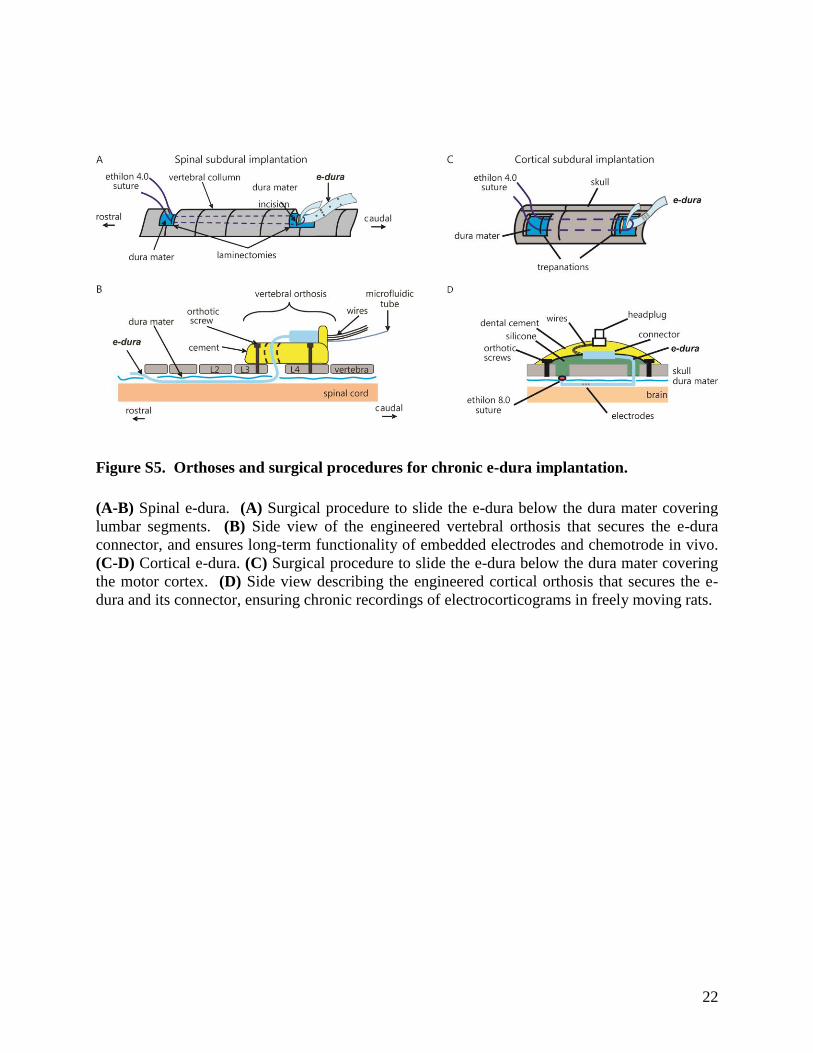
Figure S5. Orthoses and surgical procedures for chronic e-dura implantation.

(A-B) Spinal e-dura. (A) Surgical procedure to slide the e-dura below the dura mater covering

lumbar segments. (B) Side view of the engineered vertebral orthosis that secures the e-dura

connector, and ensures long-term functionality of embedded electrodes and chemotrode in vivo.

(C-D) Cortical e-dura. (C) Surgical procedure to slide the e-dura below the dura mater covering

the motor cortex. (D) Side view describing the engineered cortical orthosis that secures the e-

dura and its connector, ensuring chronic recordings of electrocorticograms in freely moving rats.

23

Figure S6. Kinematic analysis of gait patterns during basic overground locomotion.

(A) Representative stick diagram decomposition of hindlimb movement during two successive

gait cycles performed along a horizontal unobstructed runway. Recordings were obtained 6

weeks after surgery for a sham-implant rat, and for a rat implanted with an e-dura or a stiff

implant, from left to right. (B) A total of 135 parameters providing comprehensive gait

quantification (Table S1) were computed from high-resolution kinematic recordings. All the

parameters computed for a minimum of 8 gait cycles per rat at 6 weeks post-implantation were

subjected to a principal component (PC) analysis. All gait cycles (n = 102, individual dots) from

all tested rats (n = 4 per group) are represented in the new 3D space created by PC1-3, which

explained 40% of the total data variance. This analysis revealed that sham-operated rats and rats

with e-dura exhibited similar gait patterns, whereas rats with stiff implants showed markedly

different gait characteristics compared to both other groups. (C) To identify the specific features

underlying these differences, we extracted the parameters with high factor loadings on PC1, and

regrouped them into functional clusters (not shown), which we named for clarity. This analysis

revealed that rats with stiff implants displayed impaired foot control, reduced amplitude of leg

movement, and postural imbalance. To illustrate these deficits using more classic parameters,

we generated plots reporting mean values (± SEM) of variables with high factor loadings for

each of the 3 identified functional clusters. Statistical test: Kruskal-Wallis ANOVA. ***, P <

0.001. **, P < 0.01. *, P < 0.05. ns, non-significant. Error bars: standard error of mean, SEM.

24

Figure S7. Damage of spinal tissues after chronic implantation of stiff, but not soft,

implants.

3D reconstructions of lumbosacral segments for all 16 tested rats (3 groups of 4 animals),

including enhanced views. The spinal cords were explanted and reconstructed through serial

Nissl-stained cross-sections after 6-week implantation. Stiff implants induced dramatic damage

of neural tissues, whereas the soft implant had a negligible impact on the macroscopic shape of

the spinal cord. The arrowheads indicate the position of the entrance of the implant into the

subdural space.

25

Figure S8. Significant neuro-inflammatory responses after chronic implantation of stiff,

but not soft, implants.

Cross-section of the L5 lumbar segment stained for the neuro-inflammatory markers GFAP

(astrocytes) and Iba1 (microglia) after 6-week implantation. A representative photograph is

shown for each group of rats. The stiff implant leads to a dramatic increase in the density of

neuro-inflammatory cells, whereas the e-dura had a negligible impact on these responses. Scale

bars, 500µm.

26

Figure S9. Model of spinal cord and experimental quantification of vertebral column

curvatures in freely behaving rats.

(A) The mechanical model of spinal cord is composed of a hydrogel that simulates spinal tissue,

and a silicone membrane that simulates the dura mater. The soft or stiff implant was inserted

between the hydrogel and the silicone membrane. The water trapped under the simulated dura

mater ensured constant lubrication of the entire implant. Both ends of the model were sealed

with silicone forming the clamping pads used in stretching experiments. (B) To measure the

range of physiologically relevant vertebral column curvatures, we recorded spontaneous

movement of a healthy rat during exploration of a novel environment. Reflective markers were

attached overlying bony landmarks to measure motion of the vertebral column. The photographs

displayed the stereotypical motor behaviors that were extracted for further analysis. For each

behavior, we fitted a polynomial function through the inter-connected chain of markers. The

resulting curvatures are reported along the x-axis. Since the markers were attached to the

moving skin, the radii of curvature experienced by the vertebral column, and even more by the

spinal cord itself, are expected to be at least 1 to 2mm smaller. We used the measured radii of

curvature to define the bending limits applied to the spinal cord-implant model tested under

flexion.

10 20 30 40 50

Spinal radius of curvature (mm)

A

implant

hydrogel ‘spinal cord’

silicone ‘dura mater’

clamping pad 1 cm

B

27

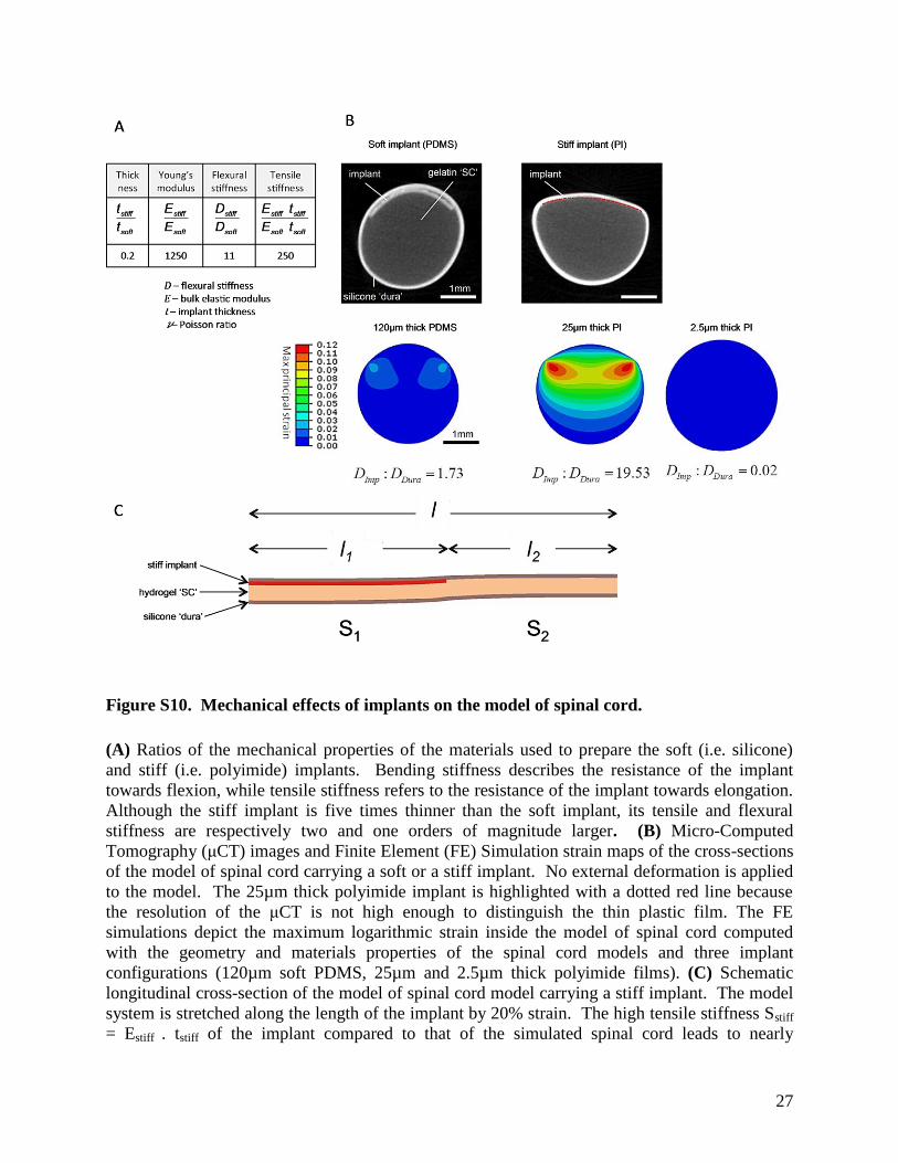
Figure S10. Mechanical effects of implants on the model of spinal cord.

(A) Ratios of the mechanical properties of the materials used to prepare the soft (i.e. silicone)

and stiff (i.e. polyimide) implants. Bending stiffness describes the resistance of the implant

towards flexion, while tensile stiffness refers to the resistance of the implant towards elongation.

Although the stiff implant is five times thinner than the soft implant, its tensile and flexural

stiffness are respectively two and one orders of magnitude larger. (B) Micro-Computed

Tomography (μCT) images and Finite Element (FE) Simulation strain maps of the cross-sections

of the model of spinal cord carrying a soft or a stiff implant. No external deformation is applied

to the model. The 25µm thick polyimide implant is highlighted with a dotted red line because

the resolution of the μCT is not high enough to distinguish the thin plastic film. The FE

simulations depict the maximum logarithmic strain inside the model of spinal cord computed

with the geometry and materials properties of the spinal cord models and three implant

configurations (120µm soft PDMS, 25µm and 2.5µm thick polyimide films). (C) Schematic

longitudinal cross-section of the model of spinal cord model carrying a stiff implant. The model

system is stretched along the length of the implant by 20% strain. The high tensile stiffness Sstiff

= Estiff . tstiff of the implant compared to that of the simulated spinal cord leads to nearly

28

unstretched simulated spinal tissues immediately underneath the implant and highly deformed

spinal tissues away from the implant.

29

Figure S11. Effect of tensile deformations on the implants and on the model of spinal cord.

(A) To measure local strains, we tracked fiducial markers in the hydrogel ‘spinal tissue’ and on

the soft or stiff implant. Graphite powder particles were mixed with the hydrogel during gel

preparation. Parallel lines with 1mm inter-distance were drawn directly onto the surface of the

implants. The model was flexed to controlled bending radii, which covered the entire range of

physiologically relevant spinal movement determined in vivo (fig. S9). The soft implant

conformed to the flexion of simulated spinal tissues. The strain along the sagittal crest of the

model (broken line) was determined experimentally (discrete symbols) and compared to a

geometrical prediction (continuous line). The stiff implant started wrinkling with radii smaller

than 30mm. The amplitude of wrinkles, termed A, and the wavelength depended on the bending

radius. (B) The spinal cord - implant model was placed under uniaxial (global) tensile stretch.

Local strain was measured by tracking the displacement of pairs of particles in the gel (n=8

pairs), or neighboring stripes on the implants (n=10 pairs). The graphs quantify locally induced

strain in the implant and in the hydrogel core (spinal tissues) as a function of the global applied

strain to the model. The soft implant stretched with the model of spinal cord. In contrast, there

was a substantial mismatch between the local strain inside the model and the induced

deformation of the stiff implant. Consequently, the stiff implant slid between the silicone and

the hydrogel during stretch. Mean ± standard deviation (SD).

30

Figure S12. Determination of charge injection capacity of electrodes with platinum-silicone

coating.

(A) Charge-balanced, biphasic current pulses were injected through electrodes immersed in

Phosphate Buffer Saline solution (PBS). The duration of each pulse phase was fixed at 200μs

per phase, which corresponds to the typical pulse duration used during therapeutic applications.

(B) The amplitude of the current pulses was gradually increased. As the current density flowing

through the coating and its polarization increased, a significant portion of the recorded voltage

drop occurred in the electrode interconnects and the electrolyte above the coating. (C) To obtain

the true voltage transients at the coating surface with respect to the reference electrode, the

instantaneous polarization of the cell was subtracted. The maximum safe current density was

reached when the coating polarization exited the water window.

31

Figure S13. Impedance spectroscopy of the soft electrodes under cyclic stretching to 20%

strain.

(A) Apparatus for conducting electrochemical characterization of soft implants under tensile

strain. The ends of the implant were glued to two probes that are clamped to the jaws of a

custom built extensimeter. The implant and (partially) the probes were then submerged in

Phosphate Buffered Saline solution (PBS). The extensimeter applied pre-defined static strain to

the implant, or performed a cyclic stretch-relax program. A counter and a reference electrode

were submerged in the electrolyte to complete the circuit (not shown). (B) Representative

impedance plots recorded from one electrode. The spectra were recorded at 0% applied strain

after 10, 1,000, 10,000, 100,000 and 1 million stretch cycles. Each stretch cycle lasted 1s. The

implants remained immersed in PBS throughout the evaluations. The remaining 6 electrodes in

the tested implants exhibited a similar behavior.

32

Figure S14. In-situ scanning electron micrographs of platinum-silicone coatings.

(A) Images collected during the first stretch cycle to 20% applied strain (from pristine electrode).

Low magnification scanning electron micrographs taken at 20% strain revealed the appearance

of cracks, but the absence of delamination. The high effective surface area of the composite

coating is clearly visible in medium magnification scanning electron micrographs (lower panels).

(B) Images collected before (cycle 0) and after one million stretch cycles to 20% strain. All the

images were taken at 0% strain. High-magnification scanning electron micrographs revealed the

effects of fatigue cycling on the nano-scale morphology of the composite coating.

33

Figure S15. Motor cortex electrocorticograms reflect motor states in freely moving rats.

(A) Raw color-coded electrocorticograms recorded against the common average for each

electrode of the chronically implanted e-dura. Colors correspond to motor states (identified from

video) and labeled as continuous walking, transition between walking and standing, and

standing. (B) Each electrocorticogram was Fourier transformed into time resolved power

spectral densities (trPSD), shown in units of standard deviation (std). (C) trPSDs averaged

across all electrodes. Each trPSD was normalized to mean trPSD in each frequency in order to

account for drop in power with increasing frequencies. The transparent regions corresponds to

the frequency sub-bands that were excluded from the analysis to remove the effect of the 50Hz

line noise and its higher order harmonics. (D) Mean ± SEM of power spectral density for

34

standing and walking states. To calculate the time-resolved power of electrocorticograms within

each contiguous band, we integrated the electrode-averaged trPSD across that band. We then

compared all time-resolved power measurements during walking periods against all time-

resolved power measurements during standing periods for each band using Wilcoxon rank-sum

test. The low (LFB) and high (HFB) frequency bands (shared areas) were identified as bands

with the local minima of p values. Histogram plots report the mean values ± SEM of electrode-

averaged power in the identified bands. ***, p < 0.001. p value corrected for multiple

comparisons using Bonferroni correction (ntests = 45,150 for each rat). (E) Electrode-averaged

trPSD, identified low and high frequency bands, and histogram plots reporting means ± SEM of

power in identified bands for walking and standing states, are shown for each rat (n = 3 rats in

total). Elevated power in low and high frequency bands during walking compared to standing is

consistent with electrocorticogram recordings during hand movements in humans (28).

35

Figure S16. Recordings of electrospinograms following peripheral nerve and brain

stimulation.

An e-dura was chronically implanted over lumbosacral segments for 6 weeks in 3 rats. Terminal

experiments were performed under urethane anesthesia. (A) Electrospinograms and left medial

gastrocnemius muscle activity were recorded in response to electrical stimulation of the left

sciatic nerve. (B) Representative color-coded electrospinograms and muscle activity responses

are displayed for increasing stimulation intensities. Electrospinograms appeared at lower

threshold than muscle responses, suggesting that e-dura electrodes measured neural activity

related to the recruitment of myelinated fibers. (C) Electrospinogram mean amplitudes for left

versus right side electrodes (10 trials per rat). Responses were significantly larger on the

stimulation side (t-test, ***, P < 0.001). (D) Correlation plot showing the relationship between

electrode location and the latency of electrospinogram responses. The locations are referred to

the left L2 electrode, which is the closest to sciatic nerve afferent neurons. The measured neural

conduction velocity from lumbar to sacral segments, which was derived from the correlation

line, is coherent with the conduction velocity of large-myelinated fibers. (E) Power spectrum of

electrospinograms is condensed in the region below 1,000Hz, which is consistent with a lead

field potential signal, most likely arising from the afferent volley and related synaptic events.

These combined results demonstrate the high degree of spatial and temporal selectivity in the

36

neural recordings obtained with e-dura. (F) A stimulating electrode was positioned over the

motor cortex of the same rats (n = 3) to elicit a descending volley. (G) Representative color-

coded recording of an electrospinogram and muscle activity following a single pulse of motor

cortex stimulation. (H) Bar plot reporting the mean (10 trials per rat) latency (± SEM) of

electrospinograms and muscle activity responses following a single pulse of stimulation.

Electrospinograms systematically preceded muscle evoked responses (t-test, *, P < 0.05). (I)

The power spectrum of electrospinograms was condensed in the region below 1,000Hz, which

was consistent with a neural response related to multiple descending pathways.

37

Figure S17. Drug delivery through the chemotrode annihilates side effects.

(A) Rats (n = 4) were tested during bipedal locomotion under robotic support after 1 week of

rehabilitation. Recordings were performed without stimulation, and with concurrent

electrochemical stimulation. Chemical stimulation was delivered either intrathecally through the

chemotrode, or intraperitonaelly. The drug volumes were adjusted to obtain the same quality of

stepping. Color-coded stick diagram decompositions of hindlimb movements are shown together

with muscle activity of antagonist ankle muscles. (B) Drug volumes required to obtain optimal

facilitation of locomotion for each serotonergic agonist. (n = 4 rats). (C) Effects of optimal drug

volumes on autonomic functions. Salivation and micturition are reported using a visual scaling

system ranging from 0 (baseline, no drug) to 5 (maximum possible effects). (n = 4 rats).

38

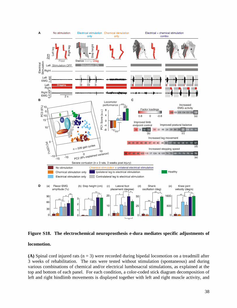
Figure S18. The electrochemical neuroprosthesis e-dura mediates specific adjustments of

locomotion.

(A) Spinal cord injured rats (n = 3) were recorded during bipedal locomotion on a treadmill after

3 weeks of rehabilitation. The rats were tested without stimulation (spontaneous) and during

various combinations of chemical and/or electrical lumbosacral stimulations, as explained at the

top and bottom of each panel. For each condition, a color-coded stick diagram decomposition of

left and right hindlimb movements is displayed together with left and right muscle activity, and

39

the color-coded duration of stance, swing, and drag phases. Without stimulation, both legs

dragged along the treadmill belt. Electrical stimulation alone delivered at the level of lumbar

(L2) and sacral (S1) electrodes, but only on the left side, induced rhythmic movement restricted

to the left leg. Chemical stimulation alone, composed of 5HT1A/7 and 5HT2 agonists, did not

induce locomotion, but raised the level of tonic muscle activity in both legs. After chemical

injection, delivery of electrical stimulation on the left side induced robust locomotor movements

restricted to the left leg. The combination of chemical and bilateral electrical stimulation

promoted coordinated locomotor movements with weight bearing, plantar placement, and

alternation of left and right leg oscillations. (B) A total of 135 parameters providing

comprehensive gait quantification (Table S1) was computed from kinematic, kinetic, and muscle

activity recordings. All the parameters were subjected to a PC analysis, as described in fig. S6.

All the gait cycles (n = 226, individual dots) from all the tested rats (n = 3) and 3 healthy rats are

represented in the new 3D space created by PC1-3, which explained nearly 50% of the total data

variance. The inset shows elliptic fitting applied on 3D clusters to emphasize the differences

between experimental conditions. The bar plot reports locomotor performance, which was

quantified as the mean values ±SEM of scores on PC1 (4). This analysis illustrates the graded

improvement of locomotor performance under the progressive combination of chemical and

bilateral electrical stimulation. Statistical test: Friedman test ANOVA. ***, P < 0.001. (C) To

identify the specific features modulated with chemical and electrical stimulation, we extracted

the parameters correlating with PC1 (factor loadings), and regrouped them into functional

clusters, which we named for clarity. The numbers refer to variables described in Table S1. (D)

Mean values ± SEM of variables with high factor loadings, for each of the 5 functional clusters,

as highlighted in panel C. Statistical test: Friedman test ANOVA. **, P < 0.01. *, P < 0.05.

Error bars: standard error of mean, SEM.

40

PARAMETERS VARIABLE DETAILED EXPLANATION

KINEMATICS

Temporal features

1 Cycle duration 2 Cycle velocity 3 Stance duration 4 Swing duration 5 Relative stance duration (percent of the cycle duration)

Limb endpoint (Metatarsal phalange) trajectory

6 Interlimb temporal coupling 7 Duration of double stance phase 8 Stride length 9 Step length 10 3D limb endpoint path length 11 Maximum backward position 12 Minimum forward position 13 Step height 14 Maximum speed during swing 15 Relative timing of maximum velocity during swing 16 Acceleration at swing onset 17 Average endpoint velocity 18 Orientation of the velocity vector at swing onset 19 Dragging 20 Relative dragging duration (percent of swing duration)

Stability

Base of support 21 Positioning of the foot at stance onset with respect to the pelvis 22 Stance width

Trunk and pelvic

position and

oscillations

23 Maximum hip sagittal position 24 Minimum hip sagittal position 25 Amplitude of sagittal hip oscillations 26 Variability of sagittal crest position 27 Variability of sagittal crest velocity 28 Variability of vertical hip movement 29 Variability of sagittal hip movement 30 Variability of the 3D hip oscillations 31 Length of pelvis displacements in the forward direction 32 Length of pelvis displacements in the medio-lateral direction 33 Length of pelvis displacements in the vertical direction 34 Length of pelvis displacements in all directions

Joint angles and segmental oscillations

Backward 35 Crest oscillations 36 Thigh oscillations 37 Leg oscillations 38 Foot oscillations 39 Whole limb oscillations

Forward 40 Crest oscillations 41 Thigh oscillations 42 Leg oscillations 43 Foot oscillations 44 Whole limb oscillations

Flexion 45 Hip joint angle 46 Knee joint angle 47 Ankle joint angle

Abduction 48 Whole limb abduction 49 Foot abduction

Extension 50 Hip joint angle 51 Knee joint angle 52 Ankle joint angle

41

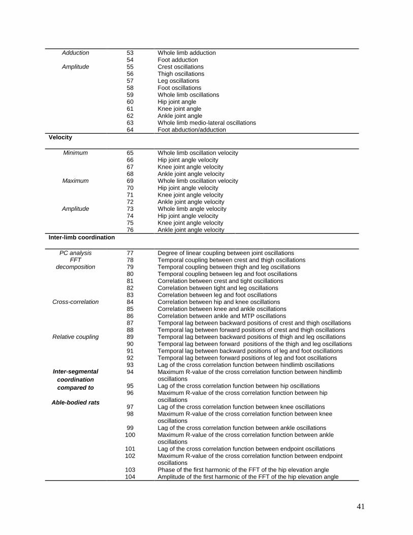
Adduction 53 Whole limb adduction 54 Foot adduction

Amplitude 55 Crest oscillations 56 Thigh oscillations 57 Leg oscillations 58 Foot oscillations 59 Whole limb oscillations 60 Hip joint angle 61 Knee joint angle 62 Ankle joint angle 63 Whole limb medio-lateral oscillations 64 Foot abduction/adduction

Velocity

Minimum 65 Whole limb oscillation velocity 66 Hip joint angle velocity 67 Knee joint angle velocity 68 Ankle joint angle velocity

Maximum 69 Whole limb oscillation velocity 70 Hip joint angle velocity 71 Knee joint angle velocity 72 Ankle joint angle velocity

Amplitude 73 Whole limb angle velocity 74 Hip joint angle velocity 75 Knee joint angle velocity 76 Ankle joint angle velocity

Inter-limb coordination

PC analysis 77 Degree of linear coupling between joint oscillations FFT

decomposition 78 Temporal coupling between crest and thigh oscillations 79 Temporal coupling between thigh and leg oscillations 80 Temporal coupling between leg and foot oscillations 81 Correlation between crest and tight oscillations 82 Correlation between tight and leg oscillations 83 Correlation between leg and foot oscillations

Cross-correlation 84 Correlation between hip and knee oscillations 85 Correlation between knee and ankle oscillations 86 Correlation between ankle and MTP oscillations 87 Temporal lag between backward positions of crest and thigh oscillations 88 Temporal lag between forward positions of crest and thigh oscillations

Relative coupling 89 Temporal lag between backward positions of thigh and leg oscillations 90 Temporal lag between forward positions of the thigh and leg oscillations 91 Temporal lag between backward positions of leg and foot oscillations 92 Temporal lag between forward positions of leg and foot oscillations

Inter-segmental

coordination

compared to

Able-bodied rats

93 Lag of the cross correlation function between hindlimb oscillations 94 Maximum R-value of the cross correlation function between hindlimb

oscillations 95 Lag of the cross correlation function between hip oscillations 96 Maximum R-value of the cross correlation function between hip

oscillations 97 Lag of the cross correlation function between knee oscillations 98 Maximum R-value of the cross correlation function between knee

oscillations 99 Lag of the cross correlation function between ankle oscillations

100 Maximum R-value of the cross correlation function between ankle oscillations

101 Lag of the cross correlation function between endpoint oscillations 102 Maximum R-value of the cross correlation function between endpoint

oscillations 103 Phase of the first harmonic of the FFT of the hip elevation angle 104 Amplitude of the first harmonic of the FFT of the hip elevation angle

42

105 Phase of the first harmonic of the FFT of the knee elevation angle 106 Amplitude of the first harmonic of the FFT of the knee elevation angle 107 Phase of the first harmonic of the FFT of the ankle elevation angle 108 Amplitude of the first harmonic of the FFT of the ankle elevation angle

Left–right

hindlimb

coordination

109 Phase of the first harmonic of the FFT of the endpoint elevation angle 110 Amplitude of the first harmonic of the FFT of the endpoint elevation angle 111 Phase of the first harmonic of the FFT of the hindlimb elevation angle 112 Amplitude of the first harmonic of the FFT of the hindlimb elevation angle 113 Lag of the cross correlation function between crest and thigh limb

elevation angles

Hindlimb

coordination

114 Lag of the cross correlation function between thigh and hindlimb elevation angles

115 Lag of the cross correlation function between hip and thigh elevation angles

116 Lag of the cross correlation function between hindlimb and foot elevation angles

117 Lag of the cross correlation function between thigh and ankle elevation angles

118 Lag of the cross correlation function between ankle and foot elevation angles

KINETICS

119 Medio-lateral forces 120 Anteroposterior forces 121 Vertical forces 122 Weight-bearing level

MUSCLE ACTIVITY

Timing (relative to cycle duration, paw contact to paw contact)

Extensor

123 Relative onset of ipsilateral extensor muscle activity burst 124 Relative end of ipsilateral extensor muscle activity burst

Flexor

125 Relative onset of ipsilateral flexor muscle activity burst 126 Relative end of ipsilateral flexor muscle activity burst

Duration

Extensor 127 Duration of ipsilateral extensor muscle activity burst Flexor 128 Duration of ipsilateral flexor muscle activity burst

Amplitude

Extensor 129 Mean amplitude of ipsilateral muscle activity burst 130 Integral of ipsilateral extensor muscle activity burst 131 Root mean square of ipsilateral extensor muscle activity burst

Flexor 132 Mean amplitude of ipsilateral flexor muscle activity burst 133 Integral of ipsilateral flexor muscle activity burst 134 Root mean square of ipsilateral flexor muscle activity burst

Muscle coactivation 135 Co-contraction of flexor and extensor muscle

Table S1: Computed kinematic, ground reaction force, and muscle activity variables.

References and Notes 1. D. Borton, S. Micera, J. R. Millán, G. Courtine, Personalized neuroprosthetics. Sci. Transl.

Med. 5, 210rv2 (2013). Medline doi:10.1126/scitranslmed.3005968

2. D.-H. Kim, J. Viventi, J. J. Amsden, J. Xiao, L. Vigeland, Y. S. Kim, J. A. Blanco, B. Panilaitis, E. S. Frechette, D. Contreras, D. L. Kaplan, F. G. Omenetto, Y. Huang, K. C. Hwang, M. R. Zakin, B. Litt, J. A. Rogers, Dissolvable films of silk fibroin for ultrathin conformal bio-integrated electronics. Nat. Mater. 9, 511–517 (2010). Medline doi:10.1038/nmat2745

3. P. Fattahi, G. Yang, G. Kim, M. R. Abidian, A review of organic and inorganic biomaterials for neural interfaces. Adv. Mater. 26, 1846–1885 (2014). Medline doi:10.1002/adma.201304496

4. R. van den Brand, J. Heutschi, Q. Barraud, J. DiGiovanna, K. Bartholdi, M. Huerlimann, L. Friedli, I. Vollenweider, E. M. Moraud, S. Duis, N. Dominici, S. Micera, P. Musienko, G. Courtine, Restoring voluntary control of locomotion after paralyzing spinal cord injury. Science 336, 1182–1185 (2012). Medline doi:10.1126/science.1217416

5. D. W. Park, A. A. Schendel, S. Mikael, S. K. Brodnick, T. J. Richner, J. P. Ness, M. R. Hayat, F. Atry, S. T. Frye, R. Pashaie, S. Thongpang, Z. Ma, J. C. Williams, Graphene-based carbon-layered electrode array technology for neural imaging and optogenetic applications. Nat. Commun. 5, 5258 (2014). Medline doi:10.1038/ncomms6258

6. J. C. Barrese, N. Rao, K. Paroo, C. Triebwasser, C. Vargas-Irwin, L. Franquemont, J. P. Donoghue, Failure mode analysis of silicon-based intracortical microelectrode arrays in non-human primates. J. Neural Eng. 10, 066014 (2013). Medline doi:10.1088/1741-2560/10/6/066014

7. P. Moshayedi, G. Ng, J. C. Kwok, G. S. Yeo, C. E. Bryant, J. W. Fawcett, K. Franze, J. Guck, The relationship between glial cell mechanosensitivity and foreign body reactions in the central nervous system. Biomaterials 35, 3919–3925 (2014). Medline doi:10.1016/j.biomaterials.2014.01.038

8. K. A. Potter, M. Jorfi, K. T. Householder, E. J. Foster, C. Weder, J. R. Capadona, Curcumin-releasing mechanically adaptive intracortical implants improve the proximal neuronal density and blood-brain barrier stability. Acta Biomater. 10, 2209–2222 (2014). Medline doi:10.1016/j.actbio.2014.01.018

9. Y.-B. Lu, K. Franze, G. Seifert, C. Steinhäuser, F. Kirchhoff, H. Wolburg, J. Guck, P. Janmey, E. Q. Wei, J. Käs, A. Reichenbach, Viscoelastic properties of individual glial cells and neurons in the CNS. Proc. Natl. Acad. Sci. U.S.A. 103, 17759–17764 (2006). Medline doi:10.1073/pnas.0606150103

10. B. S. Elkin, A. I. Ilankovan, B. Morrison 3rd, A detailed viscoelastic characterization of the P17 and adult rat brain. J. Neurotrauma 28, 2235–2244 (2011). Medline doi:10.1089/neu.2010.1604

11. A. F. Christ, K. Franze, H. Gautier, P. Moshayedi, J. Fawcett, R. J. Franklin, R. T. Karadottir, J. Guck, Mechanical difference between white and gray matter in the rat

43

cerebellum measured by scanning force microscopy. J. Biomech. 43, 2986–2992 (2010). Medline doi:10.1016/j.jbiomech.2010.07.002

12. B. S. Elkin, E. U. Azeloglu, K. D. Costa, B. Morrison 3rd, Mechanical heterogeneity of the rat hippocampus measured by atomic force microscope indentation. J. Neurotrauma 24, 812–822 (2007). Medline doi:10.1089/neu.2006.0169

13. D. R. Enzmann, N. J. Pelc, Brain motion: Measurement with phase-contrast MR imaging. Radiology 185, 653–660 (1992). Medline doi:10.1148/radiology.185.3.1438741

14. D. E. Harrison, R. Cailliet, D. D. Harrison, S. J. Troyanovich, S. O. Harrison, T. SJ, A review of biomechanics of the central nervous system—Part I: Spinal canal deformations due to changes in posture. J. Manipulative Physiol. Ther. 22, 227–234 (1999). doi:10.1016/S0161-4754(99)70049-7

15. P. Konrad, T. Shanks, Implantable brain computer interface: Challenges to neurotechnology translation. Neurobiol. Dis. 38, 369–375 (2010). Medline doi:10.1016/j.nbd.2009.12.007

16. P. Musienko, R. van den Brand, O. Maerzendorfer, A. Larmagnac, G. Courtine, Combinatory electrical and pharmacological neuroprosthetic interfaces to regain motor function after spinal cord injury. IEEE Trans. Biomed. Eng. 56, 2707–2711 (2009). Medline doi:10.1109/TBME.2009.2027226

17. S. P. Lacour, D. Chan, S. Wagner, T. Li, Z. Suo, Mechanisms of reversible stretchability of thin metal films on elastomeric substrates. Appl. Phys. Lett. 88, 204103 (2006). doi:10.1063/1.2201874

18. A. Mailis-Gagnon, A. D. Furlan, J. A. Sandoval, R. Taylor, Spinal cord stimulation for chronic pain. Cochrane Database Syst. Rev. (3): CD003783 (2004). Medline

19. C. A. Angeli, V. R. Edgerton, Y. P. Gerasimenko, S. J. Harkema, Altering spinal cord excitability enables voluntary movements after chronic complete paralysis in humans. Brain 137, 1394–1409 (2014). Medline doi:10.1093/brain/awu038

20. P. Gad, J. Choe, M. S. Nandra, H. Zhong, R. R. Roy, Y. C. Tai, V. R. Edgerton, Development of a multi-electrode array for spinal cord epidural stimulation to facilitate stepping and standing after a complete spinal cord injury in adult rats. J. Neuroeng. Rehabil. 10, 2 (2013). Medline doi:10.1186/1743-0003-10-2

21. NeuroNexus, Surface Probes. http://neuronexus.com/products/neural-probes/surface-probes, (2014).

22. C. F. Guo, T. Sun, Q. Liu, Z. Suo, Z. Ren, Highly stretchable and transparent nanomesh electrodes made by grain boundary lithography. Nat. Commun. 5, 3121 (2014). Medline doi:10.1038/ncomms4121

23. J. A. Fan, W. H. Yeo, Y. Su, Y. Hattori, W. Lee, S. Y. Jung, Y. Zhang, Z. Liu, H. Cheng, L. Falgout, M. Bajema, T. Coleman, D. Gregoire, R. J. Larsen, Y. Huang, J. A. Rogers, Fractal design concepts for stretchable electronics. Nat. Commun. 5, 3266 (2014). Medline doi:10.1038/ncomms4266

24. J. Vanfleteren, I. Chtioui, B. Plovie, Y. Yang, F. Bossuyt, T. Vervust, S. Dunphy, B. Vandecasteele, Arbitrarily Shaped 2.5D Circuits Using stretchable interconnections and

44

embedding in thermoplastic polymers. Procedia Technology 15, 208–215 (2014). doi:10.1016/j.protcy.2014.09.073

25. D.-H. Kim, R. Ghaffari, N. Lu, S. Wang, S. P. Lee, H. Keum, R. D’Angelo, L. Klinker, Y. Su, C. Lu, Y. S. Kim, A. Ameen, Y. Li, Y. Zhang, B. de Graff, Y. Y. Hsu, Z. Liu, J. Ruskin, L. Xu, C. Lu, F. G. Omenetto, Y. Huang, M. Mansour, M. J. Slepian, J. A. Rogers, Electronic sensor and actuator webs for large-area complex geometry cardiac mapping and therapy. Proc. Natl. Acad. Sci. U.S.A. 109, 19910–19915 (2012). Medline doi:10.1073/pnas.1205923109

26. S. F. Cogan, Neural stimulation and recording electrodes. Annu. Rev. Biomed. Eng. 10, 275–309 (2008). Medline doi:10.1146/annurev.bioeng.10.061807.160518

27. U. A. Aregueta-Robles, A. J. Woolley, L. A. Poole-Warren, N. H. Lovell, R. A. Green, Organic electrode coatings for next-generation neural interfaces. Frontiers in Neuroengineering 7, 15 (2014). Medline doi:10.3389/fneng.2014.00015

28. T. Pistohl, A. Schulze-Bonhage, A. Aertsen, C. Mehring, T. Ball, Decoding natural grasp types from human ECoG. Neuroimage 59, 248–260 (2012). Medline doi:10.1016/j.neuroimage.2011.06.084

29. P. Musienko, R. van den Brand, O. Märzendorfer, R. R. Roy, Y. Gerasimenko, V. R. Edgerton, G. Courtine, Controlling specific locomotor behaviors through multidimensional monoaminergic modulation of spinal circuitries. J. Neurosci. 31, 9264–9278 (2011). Medline doi:10.1523/JNEUROSCI.5796-10.2011

30. G. Courtine, Y. Gerasimenko, R. van den Brand, A. Yew, P. Musienko, H. Zhong, B. Song, Y. Ao, R. M. Ichiyama, I. Lavrov, R. R. Roy, M. V. Sofroniew, V. R. Edgerton, Transformation of nonfunctional spinal circuits into functional states after the loss of brain input. Nat. Neurosci. 12, 1333–1342 (2009). Medline doi:10.1038/nn.2401

31. L. E. Bilston, L. E. Thibault, The mechanical properties of the human cervical spinal cord in vitro. Ann. Biomed. Eng. 24, 67–74 (1996). Medline doi:10.1007/BF02770996

32. S. Cheng, E. C. Clarke, L. E. Bilston, Rheological properties of the tissues of the central nervous system: A review. Med. Eng. Phys. 30, 1318–1337 (2008). Medline doi:10.1016/j.medengphy.2008.06.003

33. T. Saxena, J. L. Gilbert, J. M. Hasenwinkel, A versatile mesoindentation system to evaluate the micromechanical properties of soft, hydrated substrates on a cellular scale. J. Biomed. Mater. Res. A 90A, 1206–1217 (2009). Medline doi:10.1002/jbm.a.32178

45