supplementary materials for: dynamic prediction of
TRANSCRIPT
1
Supplementary materials for:
Dynamic prediction of survival in cystic fibrosis:
A landmarking analysis using UK patient registry data
eAppendix 1. Creation of landmark data sets
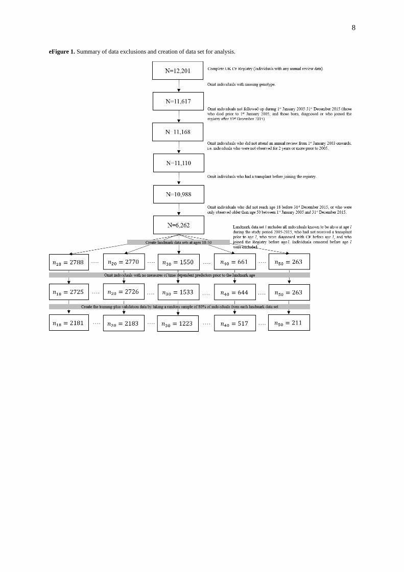
eFigure 1 illustrates how the landmark data sets arose. An individual was included in the landmark
data set at age if they met all of the following criteria:
They reached age between 1st January 2005 and 31
st December 2015.
They joined the Registry prior to reaching age . The date of joining the Registry is the date of
the first annual review at which data were obtained.
They were diagnosed with CF prior to reaching age . They have not received an organ transplant of any type prior to reaching age . They have measures of all time-dependent variables recorded prior to reaching age .
We refer to an individual as “eligible for the th landmark data set” if she/he satisfied these five
conditions. eTable 1 summarises the landmark data sets in terms of number of individuals, number of
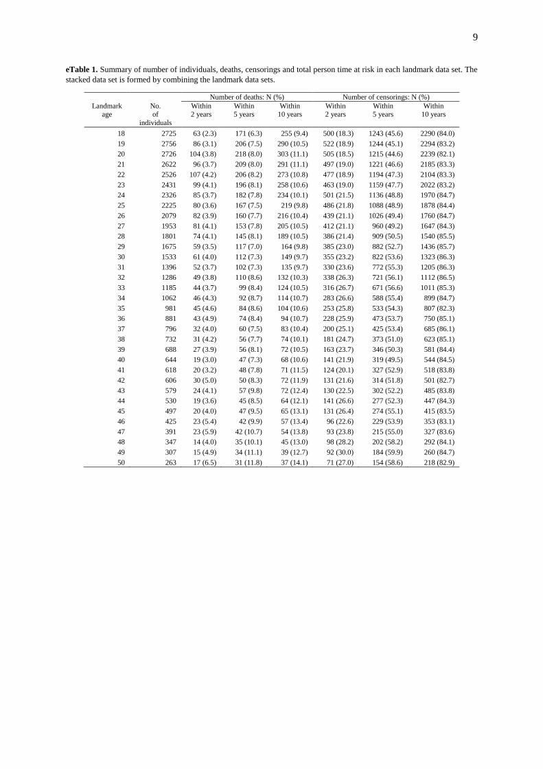
deaths within 2, 5 and 10 years of the landmark age, and number of censorings.
eAppendix 2. Survival prediction models
Time scale and follow-up
In all models the time origin is date of birth and analyses are performed using left-truncation at the
landmark age. The censoring time was the earliest of death, 31st December 2015 and a specified time
horizon . Since dates of birth and death were only available in month/year format, the day was
imputed as the 15th of the month. For example, an individual aged 18 on 1
st January 2005 (who has
been diagnosed, joined the Registry, and not received a transplant) contributes up to 11 years of
follow-up until the end of 2015 to the landmark data set for age 18 and up to 10 years of follow-up for
the landmark dataset for age 19 (if they do not die or have a transplant between ages 18 and 19), and
so on. An individual aged 18 on 1st January 2014 contributes up to 2 years of follow-up to the
landmark data set for age 18 and up to 1 year of follow-up for the landmark dataset for age 19. The UK CF Registry aims to capture deaths from all causes. Of the 931 deaths used in this study, 775
(83.2%) were due to respiratory or cardiorespiratory failure, 55 (5.9%) were transplantation-related,
13 (1.4%) were due to liver disease or failure, 9 (1.0%) were due to cancer, 9 (1.0%) were due to
trauma or suicide, 34 (3.7%) were due to “other causes” (recorded in a separate field and including
“End state cystic fibrosis” and “Haemoptysis”), 35 (3.9%) were due to an unknown cause, and for 1
individual the cause was not recorded.
We assumed that all deaths are captured and the main results presented assume censoring is entirely
administrative. In a sensitivity analysis we treated individuals not recorded at an annual follow-up for
over 2 years as lost-to-follow-up. This did not materially alter the results – the C-indexes for 2-5- and
10-year survival from the final model (Model 2) were 0.874, 0.847, 0.807 respectively, and
corresponding Brier scores were 0.036, 0.075, 0.130.
Landmark survival models
We let denote the vector of baseline predictors (sex, genotype and age of diagnosis) and denote the vector of the last-observation-carried-forward (LOCF) values for time-dependent
predictors (calendar year, FEV%, FEV%, weight, height, CFRD. pancreatic insufficiency,
Pseudomonas aeruginosa, Burkholderia cepacia, Staphylococcus aureus, Methicillin-resistant
Staphylococcus aureus (MRSA), non-IV hospitalization, number of IV days) at landmark age .
2
Model 1 for the log conditional hazard is
where is the baseline hazard at age conditional on eligibility for the th landmark data set, and
and are vectors of log hazard ratios specific to landmark age . Model 1 is in fact models,
which are fitted in each landmark data set .
Model 2 for the log conditional hazard is
where is again the baseline hazard at age conditional on eligibility for the th landmark data
set . and are vectors of log hazard ratios, which are assumed to be the same for all . Model 2 therefore allows a separate baseline hazard from each landmark age, but common predictor
coefficients across all landmark ages. It is fitted in the stacked data set using Cox regression with a
stratified baseline hazard.1,2
We note that for Models 1 and 2, using age as the time scale or time-
since-landmark as the timescale are exactly equivalent.
Models 1 and 2 make the proportional hazards assumption that the association of the predictors and with the hazard is the same over time since , i.e. that the and parameters are not time-
dependent. Models 1 and 2 were initially fitted using a time horizon of 10 years ( ), which
enables us to obtain predicted survival probabilities for any time up to 10 years. We also investigated
whether 2-year and 5-year survival could be better predicted by using a shorter time horizon by fitting
Models 1 and 2 using and respectively.
Model 3 extends Model 2 by allowing the log hazard ratios to depend on in a smooth way:
where and denote vectors of log hazard ratios that are functions of . We considered linear
forms and and restricted cubic spline forms with
knots at 18, 30, 40 and 50. The results reported in Table 3 of the main text are from the analysis using
the linear form for , as using restricted cubic splines did not materially improve predictive
performance.
In Model 4 the supermodel was extended to allow time-varying coefficients, with the association
between the predictors and the hazard dependent on time-since landmark :
where and denote vectors of log hazard ratios that are functions of . We
considered linear forms and and restricted
cubic spline forms with knots at . The results reported in Table 3 of the main text are
from the analysis using the linear form for , as using restricted cubic splines did not
materially improve predictive performance.
Model 5 uses an overall baseline hazard instead of separate baseline hazards for each landmark age,
with the impact of landmark age modelled using regression terms:
3
where is a common baseline hazard and is a function of landmark age. We used a
restricted cubic spline form for with knots at 18, 30, 40 and 50.
In Model 6 we extended Model 2 by adding the fitted values and slopes from the multivariate mixed
model (see below) for FEV%, FVC% and weight to the set of time-dependent predictors at each
landmark age:
where denotes the vector of predicted values and slopes for FEV%, FVC% and weight from the
multivariate mixed model.
All models were fitted by maximum partial likelihood.
Multivariate mixed model
A multivariate linear mixed model for FEV1%, FVC%, BMI and weight was fitted to the repeated
measures up to landmark age for individuals in the landmark data set at age . Separate
models were fitted for each landmark age. The longitudinal variables were modelled as a linear
function of age with a random intercept and slope. We also included fixed effects of all the other
predictors, including both baseline and time-dependent predictors. For each individual in landmark
dataset ( ) the individual fitted values and slopes for FEV1%, FVC% and weight at age
were obtained. The numbers of longitudinal measurements used in the multivariate mixed models are
summarised in eTable 2.
Predicted survival probabilities
From each model the predicted survival probability to time after the landmark age, conditional on
survival to the landmark age, on baseline variables and on values of time-dependent predictors at
the landmark age , , was obtained using the relationship
For models without time-varying hazard ratios (Models 1-3 and 5-6) we used the estimator:
where denotes the baseline hazard at time estimated from the increments in Breslow’s estimate
of the cumulative baseline hazard and the sum is over event times.3 For Model 4, which has time-
varying hazard ratios, we used the estimator
eAppendix 3. Model assessment
Overview
Models were assessed and compared based on the “3-in-1” procedure described by Yong et al (2013),
which incorporates model building using cross-validation, final model choice, and statistical
inference.4 The data were first divided into a “training+validation” (TV) set and a “holdout” set. The
TV set is used in the model development and assessment. The holdout set is reserved for applying the
selected model at the end. No models are fitted using the holdout data. The TV set is a sample of 80%
4
from the stacked data, stratified by landmark age. The holdout set is formed from the remaining 20%
of individuals at each landmark age. Some individuals appear in both the TV and holdout stacked data
sets, but not with the same landmark age.
For model assessment we used the C-index,5–8
the Brier score,9,10
and percentage reduction in the
Brier score relative to the null model (i.e. the model excluding all predictors, using Kaplan-Meier
estimates).11
The C-index and Brier scores were obtained using inverse probability of censoring
weights. For Model 4 we accommodated the time-varying coefficients into the estimation of the C-
Index and Brier score.8
A Monte-Carlo cross-validation procedure was used within the TV data set to avoid over-optimism
due to overfitting 12
. The procedure was as follows:
(i) An 80% stratified random sample, with stratification by landmark age , was obtained from the TV
data set.
(ii) The model was fitted on the 80% sample.
(iii) The fitted model was used to obtain predicted survival probabilities to a given time from each
landmark age (see below) for the 20% not in the sample.
(iv) Model performance measures (C-index, Brier score, and percentage reduction in the Brier score)
were obtained in the 20% not in the sample on which the model was fitted.
(v) Steps (i)-(iv) were repeated 200 times and we obtained the average C-index, Brier score and Brier
score reduction across the 200 samples.
Model assessment measures were obtained for 2-year, 5-year and 10-year survival from each
landmark age. Therefore there are 99 averaged C-indices and Brier scores for each model ( ,
where 33 is the number of landmark ages 18-50). For each model we also obtained an overall C-index
and Brier score which are not age-adjusted. Further details are given below. To simplify the notation
we give the details of the C-index and Brier score as if applied to the complete stacked data (the TV
and holdout data combined).
Truncated C-Index
The following description of the C-index follows that of Gerds et al..7 Let and denote
respectively the event time and censoring time for individual . We observe and the
event indicator . Let denote the estimated probability of survival
beyond age conditional on survival to age and given predictor values at age . The
truncated C-index is
where the expectation is with respect to two subjects , both alive at age . Not all pairs of
individuals are comparable. We can compare two individuals who both have the event prior to age
; two individuals, one of whom has the event prior to age and the other of which is known
to be alive (censored) at age . We cannot compare two individuals who are both known to be
alive (censored) at age , two individuals both censored before age , or a pair in which one
individual has the event and the other is censored before the other’s event time. The fact that not all
pairs of individuals can be compared is handled using inverse probability of censoring weights
(IPCW). The truncated C-Index can be expressed as
5
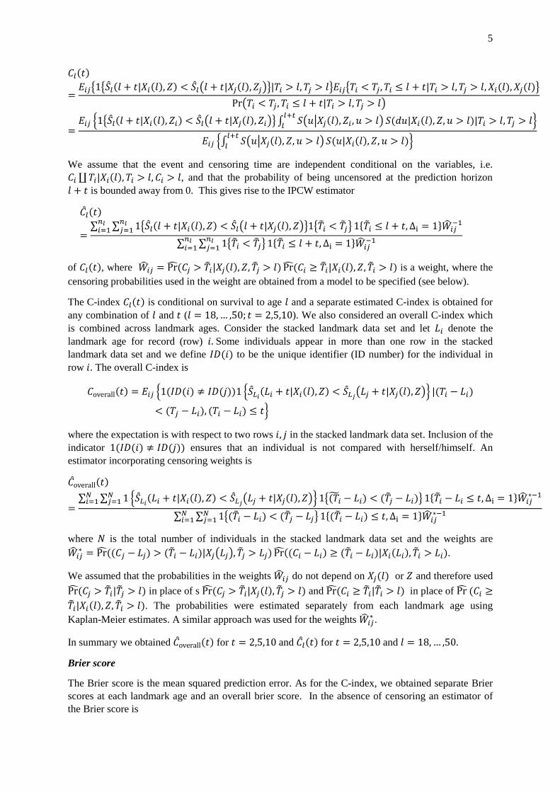
We assume that the event and censoring time are independent conditional on the variables, i.e.
, and that the probability of being uncensored at the prediction horizon
is bounded away from 0. This gives rise to the IPCW estimator
of , where is a weight, where the
censoring probabilities used in the weight are obtained from a model to be specified (see below).
The C-index is conditional on survival to age and a separate estimated C-index is obtained for
any combination of and ( ). We also considered an overall C-index which
is combined across landmark ages. Consider the stacked landmark data set and let denote the
landmark age for record (row) Some individuals appear in more than one row in the stacked
landmark data set and we define to be the unique identifier (ID number) for the individual in
row . The overall C-index is
where the expectation is with respect to two rows in the stacked landmark data set. Inclusion of the
indicator ensures that an individual is not compared with herself/himself. An
estimator incorporating censoring weights is
where is the total number of individuals in the stacked landmark data set and the weights are
.
We assumed that the probabilities in the weights do not depend on or and therefore used
in place of s and in place of
. The probabilities were estimated separately from each landmark age using
Kaplan-Meier estimates. A similar approach was used for the weights .
In summary we obtained for and for and
Brier score
The Brier score is the mean squared prediction error. As for the C-index, we obtained separate Brier
scores at each landmark age and an overall brier score. In the absence of censoring an estimator of
the Brier score is
6
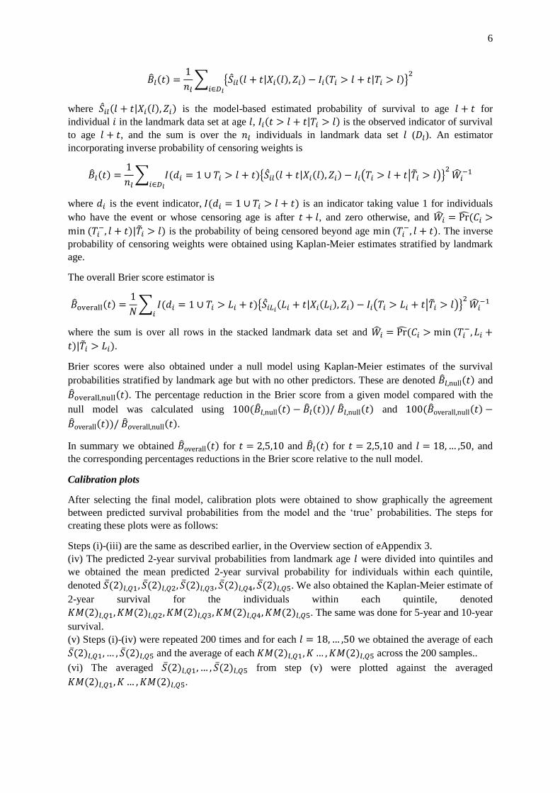
where is the model-based estimated probability of survival to age for
individual in the landmark data set at age , is the observed indicator of survival
to age , and the sum is over the individuals in landmark data set ( ). An estimator
incorporating inverse probability of censoring weights is
where is the event indicator, is an indicator taking value 1 for individuals
who have the event or whose censoring age is after , and zero otherwise, and
is the probability of being censored beyond age
. The inverse
probability of censoring weights were obtained using Kaplan-Meier estimates stratified by landmark
age.
The overall Brier score estimator is
where the sum is over all rows in the stacked landmark data set and
.
Brier scores were also obtained under a null model using Kaplan-Meier estimates of the survival
probabilities stratified by landmark age but with no other predictors. These are denoted and
. The percentage reduction in the Brier score from a given model compared with the
null model was calculated using and
.
In summary we obtained for and for and , and
the corresponding percentages reductions in the Brier score relative to the null model.
Calibration plots
After selecting the final model, calibration plots were obtained to show graphically the agreement
between predicted survival probabilities from the model and the ‘true’ probabilities. The steps for
creating these plots were as follows:
Steps (i)-(iii) are the same as described earlier, in the Overview section of eAppendix 3.
(iv) The predicted 2-year survival probabilities from landmark age were divided into quintiles and
we obtained the mean predicted 2-year survival probability for individuals within each quintile,
denoted . We also obtained the Kaplan-Meier estimate of
2-year survival for the individuals within each quintile, denoted
. The same was done for 5-year and 10-year
survival.
(v) Steps (i)-(iv) were repeated 200 times and for each we obtained the average of each
and the average of each across the 200 samples..
(vi) The averaged from step (v) were plotted against the averaged
.
7
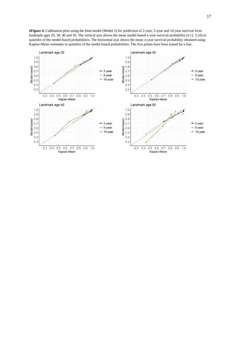
Calibration plots for landmark ages 20, 30, 40 and 50 are shown in eFigure 4. In a well-calibrated
model the five points lie on the line.
eAppendix 4. Software
All analyses were performed using R. The landmark models described in eAppendix 2 can be fitted
easily using the coxph function from the survival package after some rearrangement of the data.13
Some of the data rearrangement can be performed using the dynpred package,14
for example using the
cutLM function, though we did not use that here. Estimated survival probabilities can be obtained
using ‘predict’ after coxph, though special code was written to obtain the predicted survival
probabilities from Model 4, which included time-varying coefficients.
There exist various packages for obtaining C-indexes and Brier scores. None of the existing functions
for estimating the C-index appear to accommodate a stratified baseline hazard, and so we used
bespoke code. We used ‘pew’ from the dynpred package to estimate the Brier scores; this requires
pre-estimation of matrices of predicted survival and censoring probabilities.
The multivariate mixed model used to obtain the additional predictors for Model 6 was fitted
using the lme function from the nlme package.15
Existing software, including the nlme package, does
not appear to allow out-of-sample predictions from mixed models. We therefore used bespoke code
which is available from https://github.com/ruthkeogh/landmark_CF .
eAppendix 5. Final model specification
R code for obtaining estimated survival probabilities from the final model is provided at
https://github.com/ruthkeogh/landmark_CF. This includes csv files containing estimated cumulative
baseline hazards for each landmark age ( ).
eAppendix 6. Comparisons with other models
In an analysis of the French CF Registry Nkam et al reported a cross-validated C-statistic of 0.90 for
prediction of 3-year survival.16
They did not report a Brier score. Aside from focusing on 3-year
survival and using different set of predictors, there are a number of differences between their
approach and ours. They used a composite outcome of death and transplant, and for their logistic
regression analysis, they excluded individuals who were censored before the end of the 3-year follow-
up period.
Liou et al used a logistic regression analysis of the US CF Registry to predict 5-year survival.17
A
calibration plot showed good performance using a validation data set. However, they did not present
measures of predictive performance that are comparable to those in this paper. Mayer-Hamblett et al
also used a logistic regression analysis of the US CF Registry to develop a model for predicting 2-year
survival.18
They presented an ROC curve but did not report an area under the ROC curve, which could
be compared to our C-Index. They presented sensitivities and specificities, and positive- and negative
predictive values, finding that their model was better at predicting who would survive 2 years than
who would die.
McCarthy et al developed the CF-ABLE score using logistic regression modelling of data from the CF
population in Ireland.19
Based on a validation data set, the area under the ROC curve was 0.82 for 4-
year survival, though it is not clear how censoring was treated.
8
eFigure 1. Summary of data exclusions and creation of data set for analysis.
9
eTable 1. Summary of number of individuals, deaths, censorings and total person time at risk in each landmark data set. The
stacked data set is formed by combining the landmark data sets.
Number of deaths: N (%) Number of censorings: N (%)
Landmark age
No. of
individuals
Within 2 years
Within 5 years
Within 10 years
Within 2 years
Within 5 years
Within 10 years
18 2725 63 (2.3) 171 (6.3) 255 (9.4) 500 (18.3) 1243 (45.6) 2290 (84.0)
19 2756 86 (3.1) 206 (7.5) 290 (10.5) 522 (18.9) 1244 (45.1) 2294 (83.2)
20 2726 104 (3.8) 218 (8.0) 303 (11.1) 505 (18.5) 1215 (44.6) 2239 (82.1)
21 2622 96 (3.7) 209 (8.0) 291 (11.1) 497 (19.0) 1221 (46.6) 2185 (83.3)
22 2526 107 (4.2) 206 (8.2) 273 (10.8) 477 (18.9) 1194 (47.3) 2104 (83.3)
23 2431 99 (4.1) 196 (8.1) 258 (10.6) 463 (19.0) 1159 (47.7) 2022 (83.2)
24 2326 85 (3.7) 182 (7.8) 234 (10.1) 501 (21.5) 1136 (48.8) 1970 (84.7)
25 2225 80 (3.6) 167 (7.5) 219 (9.8) 486 (21.8) 1088 (48.9) 1878 (84.4)
26 2079 82 (3.9) 160 (7.7) 216 (10.4) 439 (21.1) 1026 (49.4) 1760 (84.7)
27 1953 81 (4.1) 153 (7.8) 205 (10.5) 412 (21.1) 960 (49.2) 1647 (84.3)
28 1801 74 (4.1) 145 (8.1) 189 (10.5) 386 (21.4) 909 (50.5) 1540 (85.5)
29 1675 59 (3.5) 117 (7.0) 164 (9.8) 385 (23.0) 882 (52.7) 1436 (85.7)
30 1533 61 (4.0) 112 (7.3) 149 (9.7) 355 (23.2) 822 (53.6) 1323 (86.3)
31 1396 52 (3.7) 102 (7.3) 135 (9.7) 330 (23.6) 772 (55.3) 1205 (86.3)
32 1286 49 (3.8) 110 (8.6) 132 (10.3) 338 (26.3) 721 (56.1) 1112 (86.5)
33 1185 44 (3.7) 99 (8.4) 124 (10.5) 316 (26.7) 671 (56.6) 1011 (85.3)
34 1062 46 (4.3) 92 (8.7) 114 (10.7) 283 (26.6) 588 (55.4) 899 (84.7)
35 981 45 (4.6) 84 (8.6) 104 (10.6) 253 (25.8) 533 (54.3) 807 (82.3)
36 881 43 (4.9) 74 (8.4) 94 (10.7) 228 (25.9) 473 (53.7) 750 (85.1)
37 796 32 (4.0) 60 (7.5) 83 (10.4) 200 (25.1) 425 (53.4) 685 (86.1)
38 732 31 (4.2) 56 (7.7) 74 (10.1) 181 (24.7) 373 (51.0) 623 (85.1)
39 688 27 (3.9) 56 (8.1) 72 (10.5) 163 (23.7) 346 (50.3) 581 (84.4)
40 644 19 (3.0) 47 (7.3) 68 (10.6) 141 (21.9) 319 (49.5) 544 (84.5)
41 618 20 (3.2) 48 (7.8) 71 (11.5) 124 (20.1) 327 (52.9) 518 (83.8)
42 606 30 (5.0) 50 (8.3) 72 (11.9) 131 (21.6) 314 (51.8) 501 (82.7)
43 579 24 (4.1) 57 (9.8) 72 (12.4) 130 (22.5) 302 (52.2) 485 (83.8)
44 530 19 (3.6) 45 (8.5) 64 (12.1) 141 (26.6) 277 (52.3) 447 (84.3)
45 497 20 (4.0) 47 (9.5) 65 (13.1) 131 (26.4) 274 (55.1) 415 (83.5)
46 425 23 (5.4) 42 (9.9) 57 (13.4) 96 (22.6) 229 (53.9) 353 (83.1)
47 391 23 (5.9) 42 (10.7) 54 (13.8) 93 (23.8) 215 (55.0) 327 (83.6)
48 347 14 (4.0) 35 (10.1) 45 (13.0) 98 (28.2) 202 (58.2) 292 (84.1)
49 307 15 (4.9) 34 (11.1) 39 (12.7) 92 (30.0) 184 (59.9) 260 (84.7)
50 263 17 (6.5) 31 (11.8) 37 (14.1) 71 (27.0) 154 (58.6) 218 (82.9)
10
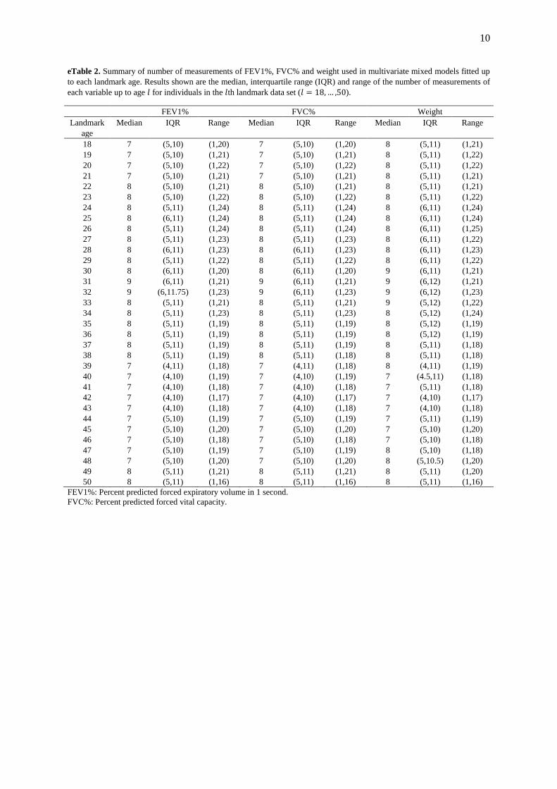
eTable 2. Summary of number of measurements of FEV1%, FVC% and weight used in multivariate mixed models fitted up
to each landmark age. Results shown are the median, interquartile range (IQR) and range of the number of measurements of
each variable up to age for individuals in the th landmark data set ( ).
FEV1% FVC% Weight
Landmark
age
Median IQR Range Median IQR Range Median IQR Range
18 7 (5,10) (1,20) 7 (5,10) (1,20) 8 (5,11) (1,21)
19 7 (5,10) (1,21) 7 (5,10) (1,21) 8 (5,11) (1,22)
20 7 (5,10) (1,22) 7 (5,10) (1,22) 8 (5,11) (1,22)
21 7 (5,10) (1,21) 7 (5,10) (1,21) 8 (5,11) (1,21)
22 8 (5,10) (1,21) 8 (5,10) (1,21) 8 (5,11) (1,21)
23 8 (5,10) (1,22) 8 (5,10) (1,22) 8 (5,11) (1,22)
24 8 (5,11) (1,24) 8 (5,11) (1,24) 8 (6,11) (1,24)
25 8 (6,11) (1,24) 8 (5,11) (1,24) 8 (6,11) (1,24)
26 8 (5,11) (1,24) 8 (5,11) (1,24) 8 (6,11) (1,25)
27 8 (5,11) (1,23) 8 (5,11) (1,23) 8 (6,11) (1,22)
28 8 (6,11) (1,23) 8 (6,11) (1,23) 8 (6,11) (1,23)
29 8 (5,11) (1,22) 8 (5,11) (1,22) 8 (6,11) (1,22)
30 8 (6,11) (1,20) 8 (6,11) (1,20) 9 (6,11) (1,21)
31 9 (6,11) (1,21) 9 (6,11) (1,21) 9 (6,12) (1,21)
32 9 (6,11.75) (1,23) 9 (6,11) (1,23) 9 (6,12) (1,23)
33 8 (5,11) (1,21) 8 (5,11) (1,21) 9 (5,12) (1,22)
34 8 (5,11) (1,23) 8 (5,11) (1,23) 8 (5,12) (1,24)
35 8 (5,11) (1,19) 8 (5,11) (1,19) 8 (5,12) (1,19)
36 8 (5,11) (1,19) 8 (5,11) (1,19) 8 (5,12) (1,19)
37 8 (5,11) (1,19) 8 (5,11) (1,19) 8 (5,11) (1,18)
38 8 (5,11) (1,19) 8 (5,11) (1,18) 8 (5,11) (1,18)
39 7 (4,11) (1,18) 7 (4,11) (1,18) 8 (4,11) (1,19)
40 7 (4,10) (1,19) 7 (4,10) (1,19) 7 (4.5,11) (1,18)
41 7 (4,10) (1,18) 7 (4,10) (1,18) 7 (5,11) (1,18)
42 7 (4,10) (1,17) 7 (4,10) (1,17) 7 (4,10) (1,17)
43 7 (4,10) (1,18) 7 (4,10) (1,18) 7 (4,10) (1,18)
44 7 (5,10) (1,19) 7 (5,10) (1,19) 7 (5,11) (1,19)
45 7 (5,10) (1,20) 7 (5,10) (1,20) 7 (5,10) (1,20)
46 7 (5,10) (1,18) 7 (5,10) (1,18) 7 (5,10) (1,18)
47 7 (5,10) (1,19) 7 (5,10) (1,19) 8 (5,10) (1,18)
48 7 (5,10) (1,20) 7 (5,10) (1,20) 8 (5,10.5) (1,20)
49 8 (5,11) (1,21) 8 (5,11) (1,21) 8 (5,11) (1,20)
50 8 (5,11) (1,16) 8 (5,11) (1,16) 8 (5,11) (1,16)
FEV1%: Percent predicted forced expiratory volume in 1 second.
FVC%: Percent predicted forced vital capacity.
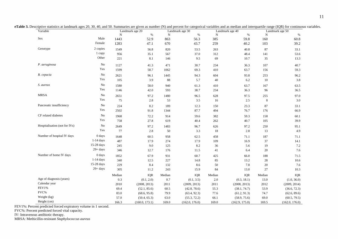
11 eTable 3. Descriptive statistics at landmark ages 20, 30, 40, and 50. Summaries are given as number (N) and percent for categorical variables and as median and interquartile range (IQR) for continuous variables.
Variable Landmark age 20 Landmark age 30 Landmark age 40 Landmark age 50 N % N % N % N %
Sex Male 1443 52.9 863 56.3 385 59.8 160 60.8 Female 1283 47.1 670 43.7 259 40.2 103 39.2 Genotype 2 copies 1549 56.8 820 53.5 263 40.8 87 33.1
1 copy 956 35.1 567 37.0 312 48.4 141 53.6
Other 221 8.1 146 9.5 69 10.7 35 13.3 P. aeruginosa No 1127 41.3 471 30.7 234 36.3 107 40.7
Yes 1599 58.7 1062 69.3 410 63.7 156 59.3 B. cepacia No 2621 96.1 1445 94.3 604 93.8 253 96.2
Yes 105 3.9 88 5.7 40 6.2 10 3.8
S. aureus No 1580 58.0 940 61.3 410 63.7 167 63.5
Yes 1146 42.0 593 38.7 234 36.3 96 36.5
MRSA No 2651 97.2 1480 96.5 628 97.5 255 97.0 Yes 75 2.8 53 3.5 16 2.5 8 3.0
Pancreatic insufficiency No 224 8.2 189 12.3 150 23.3 87 33.1
Yes 2502 91.8 1344 87.7 494 76.7 176 66.9 CF related diabetes No 1968 72.2 914 59.6 382 59.3 158 60.1
Yes 758 27.8 619 40.4 262 40.7 105 39.9
Hospitalisation (not for IVs) No 2649 97.2 1483 96.7 626 97.2 250 95.1
Yes 77 2.8 50 3.3 18 2.8 13 4.9
Number of hospital IV days 0 days 1648 60.5 958 62.5 458 71.1 187 71.1 1-14 days 487 17.9 274 17.9 109 16.9 37 14.1
15-28 days 245 9.0 125 8.2 36 5.6 19 7.2
29+ days 346 12.7 176 11.5 41 6.4 20 7.6
Number of home IV days 0 days 1852 67.9 931 60.7 425 66.0 188 71.5
1-14 days 340 12.5 227 14.8 85 13.2 28 10.6
15-28 days 229 8.4 132 8.6 50 7.8 20 7.6
29+ days 305 11.2 243 15.9 84 13.0 27 10.3 Median IQR Median IQR Median IQR Median IQR
Age of diagnosis (years) 0.3 (0.1, 2.0) 0.7 (0.1, 3.5) 2.0 (0.3, 18.1) 13.0 (1.0, 36.0)
Calendar year 2010 (2008, 2013) 2011 (2009, 2013) 2011 (2008, 2013) 2012 (2009, 2014) FEV1% 69.4 (52.1, 85.6) 60.5 (42.8, 78.6) 55.3 (38.1, 74.7) 53.9 (36.6, 72.3)
FVC% 83.0 (68.6, 95.8) 79.9 (63.4, 92.3) 77.6 (61.2, 91.3) 74.7 (62.6, 89.6)
Weight (kg) 57.0 (50.4, 65.3) 63.0 (55.3, 72.2) 66.1 (58.9, 75.6) 69.0 (60.5, 79.5)
Height (cm) 166.3 (160.0, 173.1) 169.0 (162.0, 176.0) 169.0 (162.9, 175.0) 169.5 (162.0, 176.0)
FEV1%: Percent predicted forced expiratory volume in 1 second.
FVC%: Percent predicted forced vital capacity.
IV: Intravenous antibiotic therapy.
MRSA: Methicillin-resistant Staphylococcus aureus

12
13
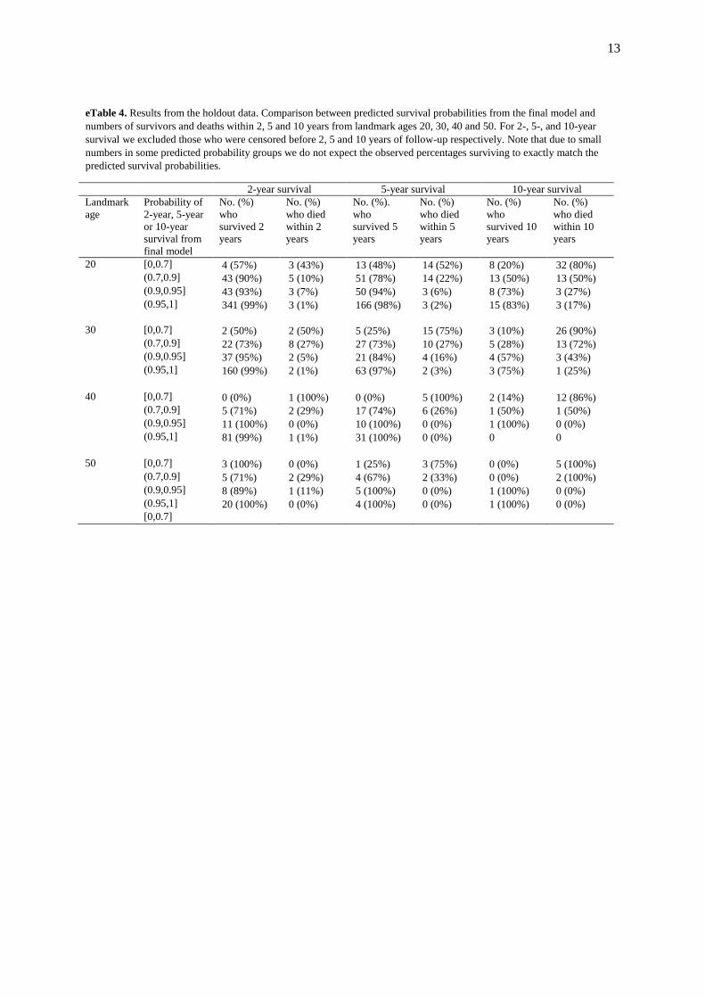
eTable 4. Results from the holdout data. Comparison between predicted survival probabilities from the final model and
numbers of survivors and deaths within 2, 5 and 10 years from landmark ages 20, 30, 40 and 50. For 2-, 5-, and 10-year
survival we excluded those who were censored before 2, 5 and 10 years of follow-up respectively. Note that due to small
numbers in some predicted probability groups we do not expect the observed percentages surviving to exactly match the
predicted survival probabilities.
2-year survival 5-year survival 10-year survival
Landmark
age
Probability of
2-year, 5-year
or 10-year
survival from
final model
No. (%)
who
survived 2
years
No. (%)
who died
within 2
years
No. (%).
who
survived 5
years
No. (%)
who died
within 5
years
No. (%)
who
survived 10
years
No. (%)
who died
within 10
years
20 [0,0.7] 4 (57%) 3 (43%) 13 (48%) 14 (52%) 8 (20%) 32 (80%)
(0.7,0.9] 43 (90%) 5 (10%) 51 (78%) 14 (22%) 13 (50%) 13 (50%)
(0.9,0.95] 43 (93%) 3 (7%) 50 (94%) 3 (6%) 8 (73%) 3 (27%)
(0.95,1] 341 (99%) 3 (1%) 166 (98%) 3 (2%) 15 (83%) 3 (17%)
30 [0,0.7] 2 (50%) 2 (50%) 5 (25%) 15 (75%) 3 (10%) 26 (90%)
(0.7,0.9] 22 (73%) 8 (27%) 27 (73%) 10 (27%) 5 (28%) 13 (72%)
(0.9,0.95] 37 (95%) 2 (5%) 21 (84%) 4 (16%) 4 (57%) 3 (43%)
(0.95,1] 160 (99%) 2 (1%) 63 (97%) 2 (3%) 3 (75%) 1 (25%)
40 [0,0.7] 0 (0%) 1 (100%) 0 (0%) 5 (100%) 2 (14%) 12 (86%)
(0.7,0.9] 5 (71%) 2 (29%) 17 (74%) 6 (26%) 1 (50%) 1 (50%)
(0.9,0.95] 11 (100%) 0 (0%) 10 (100%) 0 (0%) 1 (100%) 0 (0%)
(0.95,1] 81 (99%) 1 (1%) 31 (100%) 0 (0%) 0 0
50 [0,0.7] 3 (100%) 0 (0%) 1 (25%) 3 (75%) 0 (0%) 5 (100%)
(0.7,0.9] 5 (71%) 2 (29%) 4 (67%) 2 (33%) 0 (0%) 2 (100%)
(0.9,0.95] 8 (89%) 1 (11%) 5 (100%) 0 (0%) 1 (100%) 0 (0%)
(0.95,1] 20 (100%) 0 (0%) 4 (100%) 0 (0%) 1 (100%) 0 (0%)
[0,0.7]
14
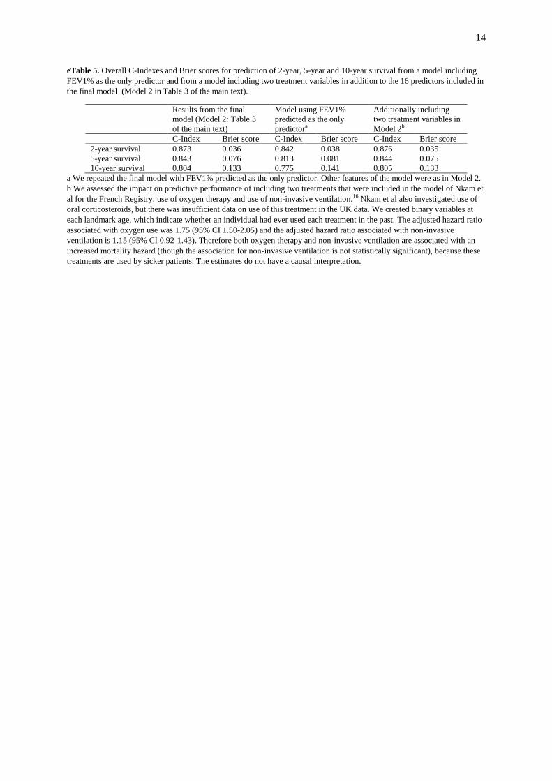
eTable 5. Overall C-Indexes and Brier scores for prediction of 2-year, 5-year and 10-year survival from a model including
FEV1% as the only predictor and from a model including two treatment variables in addition to the 16 predictors included in
the final model (Model 2 in Table 3 of the main text).
Results from the final
model (Model 2: Table 3
of the main text)
Model using FEV1%
predicted as the only
predictora
Additionally including
two treatment variables in
Model 2b
C-Index Brier score C-Index Brier score C-Index Brier score
2-year survival 0.873 0.036 0.842 0.038 0.876 0.035
5-year survival 0.843 0.076 0.813 0.081 0.844 0.075
10-year survival 0.804 0.133 0.775 0.141 0.805 0.133
a We repeated the final model with FEV1% predicted as the only predictor. Other features of the model were as in Model 2.
b We assessed the impact on predictive performance of including two treatments that were included in the model of Nkam et
al for the French Registry: use of oxygen therapy and use of non-invasive ventilation.16 Nkam et al also investigated use of
oral corticosteroids, but there was insufficient data on use of this treatment in the UK data. We created binary variables at
each landmark age, which indicate whether an individual had ever used each treatment in the past. The adjusted hazard ratio
associated with oxygen use was 1.75 (95% CI 1.50-2.05) and the adjusted hazard ratio associated with non-invasive
ventilation is 1.15 (95% CI 0.92-1.43). Therefore both oxygen therapy and non-invasive ventilation are associated with an
increased mortality hazard (though the association for non-invasive ventilation is not statistically significant), because these
treatments are used by sicker patients. The estimates do not have a causal interpretation.
15
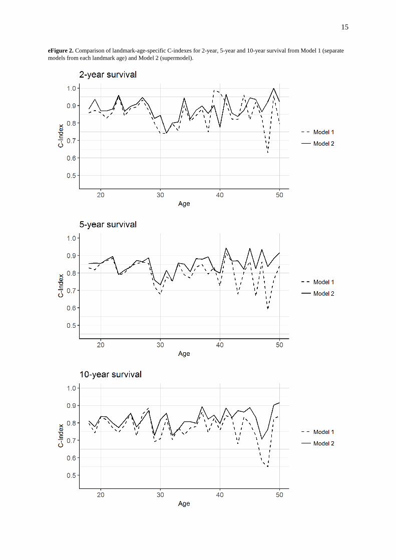
eFigure 2. Comparison of landmark-age-specific C-indexes for 2-year, 5-year and 10-year survival from Model 1 (separate
models from each landmark age) and Model 2 (supermodel).
16
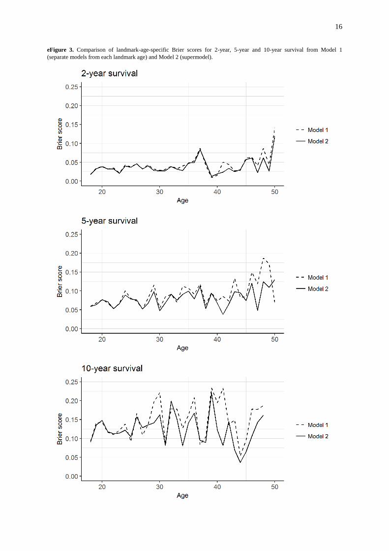
eFigure 3. Comparison of landmark-age-specific Brier scores for 2-year, 5-year and 10-year survival from Model 1
(separate models from each landmark age) and Model 2 (supermodel).
17
eFigure 4. Calibration plots using the final model (Model 2) for prediction of 2-year, 5-year and 10-year survival from
landmark ages 20, 30, 40 and 50. The vertical axis shows the mean model-based x-year survival probability (x=2, 5,10) in
quintiles of the model-based probabilities. The horizontal axis shows the mean x-year survival probability obtained using
Kaplan-Meier estimates in quintiles of the model-based probabilities. The five points have been joined by a line.
18
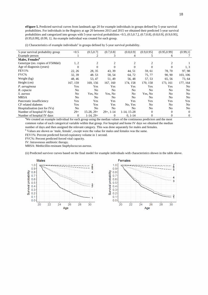
eFigure 5. Predicted survival curves from landmark age 20 for example individuals in groups defined by 5-year survival
probabilities. For individuals in the Registry at age 20 between 2013 and 2015 we obtained their predicted 5-year survival
probabilities and categorized into groups with 5-year survival probabilities <0.5, (0.5,0.7,], (0.7,0.8], (0.8,0.9], (0.9,0.95],
(0.95,0.99], (0.99, 1]. An example individual was created for each group.
(i) Characteristics of example individualsa in groups defined by 5-year survival probability.
5-year survival probability group <0.5 (0.5,0.7] (0.7,0.8] (0.8,0.9] (0.9,0.95] (0.95,0.99] (0.99,1]
Example person 1 2 3 4 5 6 7
Males, Femalesb
Genotype (no. copies of F508del) 1, 2 2 2 2 2 2 1
Age of diagnosis (years) 0 0 0 0 0 0 1, 3
FEV1% 22, 26 28, 35 43, 39 44, 51 59, 61 78, 70 97, 98
FVC% 32, 39 48. 53 58, 54 64, 72 75, 77 90, 90 103, 106
Weight (kg) 48, 46 53, 47 51, 49 56, 48 57, 53 65, 56 73, 64
Height (cm) 167, 159 169, 156 167, 160 174, 158 170, 158 173, 161 177, 164
P. aeruginosa Yes Yes Yes Yes Yes Yes No
B. cepacia No No No No No No No
S. aureus No Yes, No Yes, No No Yes, No No No
MRSA No No No No No No No
Pancreatic insufficiency Yes Yes Yes Yes Yes Yes Yes
CF related diabetes Yes Yes Yes No, Yes No No No
Hospitalisation (not for IVs) No No No No No No No
Number of hospital IV days 29+ 15-28, 29+ 29+, 1-14 1-14, 15-28 0 0 0
Number of hospital IV days 0 1-14, 29+ 0 0, 1-14 0 0 0 aWe created an example individual for each group using the median values of the continuous predictors and the most
common value of each categorical variable within that group. For hospital and home IV days we obtained the median
number of days and then assigned the relevant category. This was done separately for males and females. b Values are shown as ‘male, female’, except were the value for males and females was the same.
FEV1%: Percent predicted forced expiratory volume in 1 second.
FVC%: Percent predicted forced vital capacity.
IV: Intravenous antibiotic therapy.
MRSA: Methicillin-resistant Staphylococcus aureus.
(ii) Predicted survivor curves based on the final model for example individuals with characteristics shown in the table above.
19
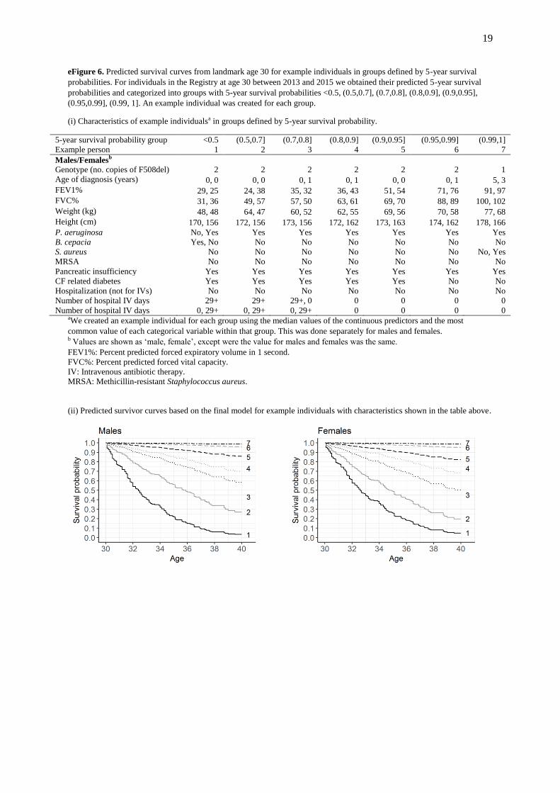
eFigure 6. Predicted survival curves from landmark age 30 for example individuals in groups defined by 5-year survival
probabilities. For individuals in the Registry at age 30 between 2013 and 2015 we obtained their predicted 5-year survival
probabilities and categorized into groups with 5-year survival probabilities <0.5, (0.5,0.7], (0.7,0.8], (0.8,0.9], (0.9,0.95],
(0.95,0.99], (0.99, 1]. An example individual was created for each group.
(i) Characteristics of example individualsa in groups defined by 5-year survival probability.
5-year survival probability group <0.5 (0.5,0.7] (0.7,0.8] (0.8,0.9] (0.9,0.95] (0.95,0.99] (0.99,1]
Example person 1 2 3 4 5 6 7
Males/Femalesb
Genotype (no. copies of F508del) 2 2 2 2 2 2 1
Age of diagnosis (years) 0, 0 0, 0 0, 1 0, 1 0, 0 0, 1 5, 3
FEV1% 29, 25 24, 38 35, 32 36, 43 51, 54 71, 76 91, 97
FVC% 31, 36 49, 57 57, 50 63, 61 69, 70 88, 89 100, 102
Weight (kg) 48, 48 64, 47 60, 52 62, 55 69, 56 70, 58 77, 68
Height (cm) 170, 156 172, 156 173, 156 172, 162 173, 163 174, 162 178, 166
P. aeruginosa No, Yes Yes Yes Yes Yes Yes Yes
B. cepacia Yes, No No No No No No No
S. aureus No No No No No No No, Yes
MRSA No No No No No No No
Pancreatic insufficiency Yes Yes Yes Yes Yes Yes Yes
CF related diabetes Yes Yes Yes Yes Yes No No
Hospitalization (not for IVs) No No No No No No No
Number of hospital IV days 29+ 29+ 29+, 0 0 0 0 0
Number of hospital IV days 0, 29+ 0, 29+ 0, 29+ 0 0 0 0 aWe created an example individual for each group using the median values of the continuous predictors and the most
common value of each categorical variable within that group. This was done separately for males and females. b Values are shown as ‘male, female’, except were the value for males and females was the same.
FEV1%: Percent predicted forced expiratory volume in 1 second.
FVC%: Percent predicted forced vital capacity.
IV: Intravenous antibiotic therapy.
MRSA: Methicillin-resistant Staphylococcus aureus.
(ii) Predicted survivor curves based on the final model for example individuals with characteristics shown in the table above.
20
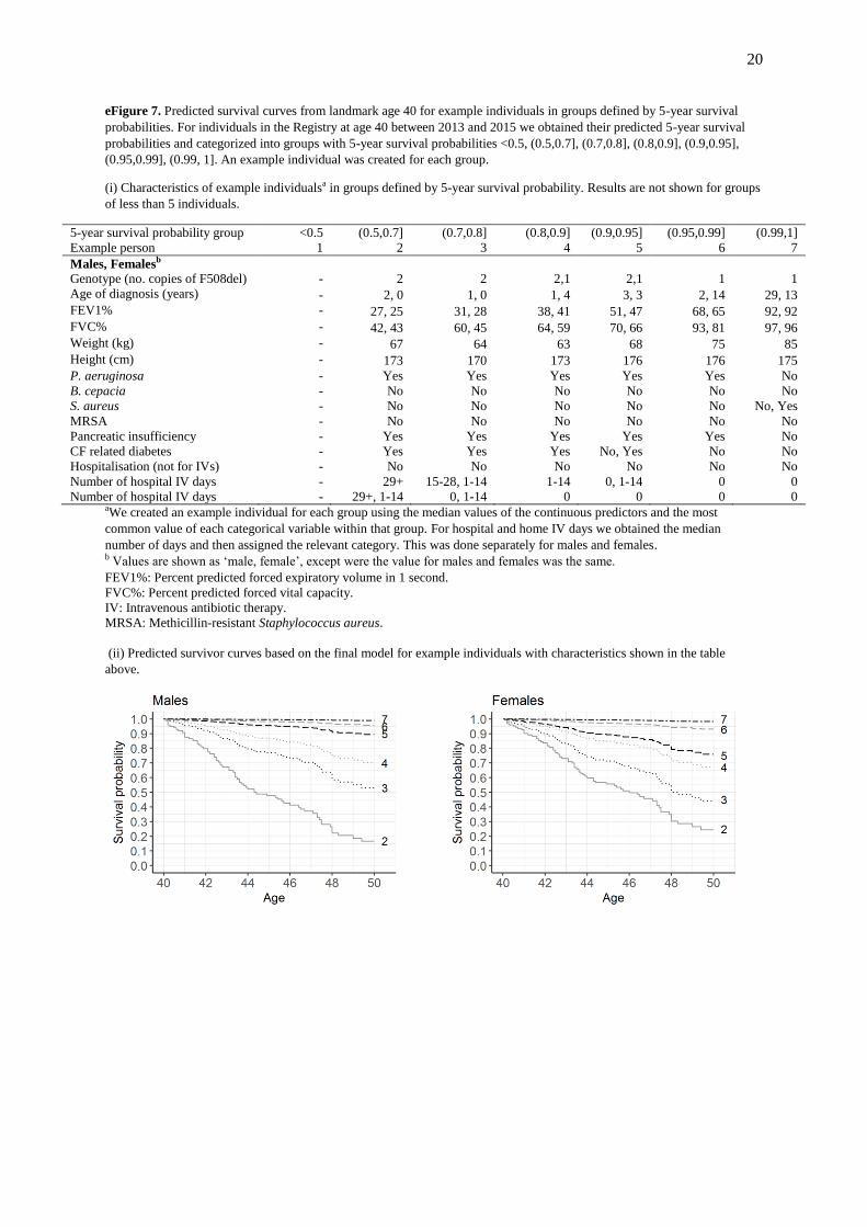
eFigure 7. Predicted survival curves from landmark age 40 for example individuals in groups defined by 5-year survival
probabilities. For individuals in the Registry at age 40 between 2013 and 2015 we obtained their predicted 5-year survival
probabilities and categorized into groups with 5-year survival probabilities <0.5, (0.5,0.7], (0.7,0.8], (0.8,0.9], (0.9,0.95],
(0.95,0.99], (0.99, 1]. An example individual was created for each group.
(i) Characteristics of example individualsa in groups defined by 5-year survival probability. Results are not shown for groups
of less than 5 individuals.
5-year survival probability group <0.5 (0.5,0.7] (0.7,0.8] (0.8,0.9] (0.9,0.95] (0.95,0.99] (0.99,1]
Example person 1 2 3 4 5 6 7
Males, Femalesb
Genotype (no. copies of F508del) - 2 2 2,1 2,1 1 1
Age of diagnosis (years) - 2, 0 1, 0 1, 4 3, 3 2, 14 29, 13
FEV1% - 27, 25 31, 28 38, 41 51, 47 68, 65 92, 92
FVC% - 42, 43 60, 45 64, 59 70, 66 93, 81 97, 96
Weight (kg) - 67 64 63 68 75 85
Height (cm) - 173 170 173 176 176 175
P. aeruginosa - Yes Yes Yes Yes Yes No
B. cepacia - No No No No No No
S. aureus - No No No No No No, Yes
MRSA - No No No No No No
Pancreatic insufficiency - Yes Yes Yes Yes Yes No
CF related diabetes - Yes Yes Yes No, Yes No No
Hospitalisation (not for IVs) - No No No No No No
Number of hospital IV days - 29+ 15-28, 1-14 1-14 0, 1-14 0 0
Number of hospital IV days - 29+, 1-14 0, 1-14 0 0 0 0 aWe created an example individual for each group using the median values of the continuous predictors and the most
common value of each categorical variable within that group. For hospital and home IV days we obtained the median
number of days and then assigned the relevant category. This was done separately for males and females. b Values are shown as ‘male, female’, except were the value for males and females was the same.
FEV1%: Percent predicted forced expiratory volume in 1 second.
FVC%: Percent predicted forced vital capacity.
IV: Intravenous antibiotic therapy.
MRSA: Methicillin-resistant Staphylococcus aureus.
(ii) Predicted survivor curves based on the final model for example individuals with characteristics shown in the table
above.
21
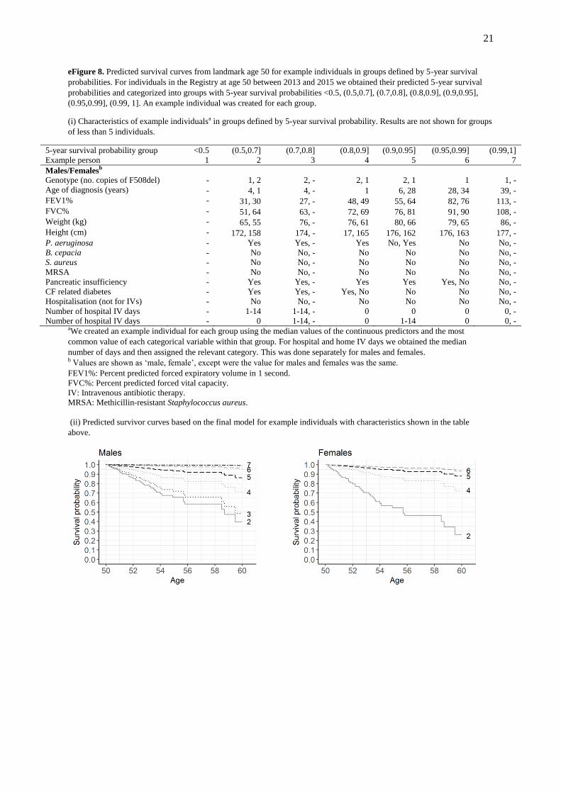
eFigure 8. Predicted survival curves from landmark age 50 for example individuals in groups defined by 5-year survival
probabilities. For individuals in the Registry at age 50 between 2013 and 2015 we obtained their predicted 5-year survival
probabilities and categorized into groups with 5-year survival probabilities <0.5, (0.5,0.7], (0.7,0.8], (0.8,0.9], (0.9,0.95],
(0.95,0.99], (0.99, 1]. An example individual was created for each group.
(i) Characteristics of example individualsa in groups defined by 5-year survival probability. Results are not shown for groups
of less than 5 individuals.
5-year survival probability group <0.5 (0.5,0.7] (0.7,0.8] (0.8,0.9] (0.9,0.95] (0.95,0.99] (0.99,1]
Example person 1 2 3 4 5 6 7
Males/Femalesb
Genotype (no. copies of F508del) - 1, 2 2, - 2, 1 2, 1 1 1, -
Age of diagnosis (years) - 4, 1 4, - 1 6, 28 28, 34 39, -
FEV1% - 31, 30 27, - 48, 49 55, 64 82, 76 113, -
FVC% - 51, 64 63, - 72, 69 76, 81 91, 90 108, -
Weight (kg) - 65, 55 76, - 76, 61 80, 66 79, 65 86, -
Height (cm) - 172, 158 174, - 17, 165 176, 162 176, 163 177, -
P. aeruginosa - Yes Yes, - Yes No, Yes No No, -
B. cepacia - No No, - No No No No, -
S. aureus - No No, - No No No No, -
MRSA - No No, - No No No No, -
Pancreatic insufficiency - Yes Yes, - Yes Yes Yes, No No, -
CF related diabetes - Yes Yes, - Yes, No No No No, -
Hospitalisation (not for IVs) - No No, - No No No No, -
Number of hospital IV days - 1-14 1-14, - 0 0 0 0, -
Number of hospital IV days - 0 1-14, - 0 1-14 0 0, - aWe created an example individual for each group using the median values of the continuous predictors and the most
common value of each categorical variable within that group. For hospital and home IV days we obtained the median
number of days and then assigned the relevant category. This was done separately for males and females. b Values are shown as ‘male, female’, except were the value for males and females was the same.
FEV1%: Percent predicted forced expiratory volume in 1 second.
FVC%: Percent predicted forced vital capacity.
IV: Intravenous antibiotic therapy.
MRSA: Methicillin-resistant Staphylococcus aureus.
(ii) Predicted survivor curves based on the final model for example individuals with characteristics shown in the table
above.
22
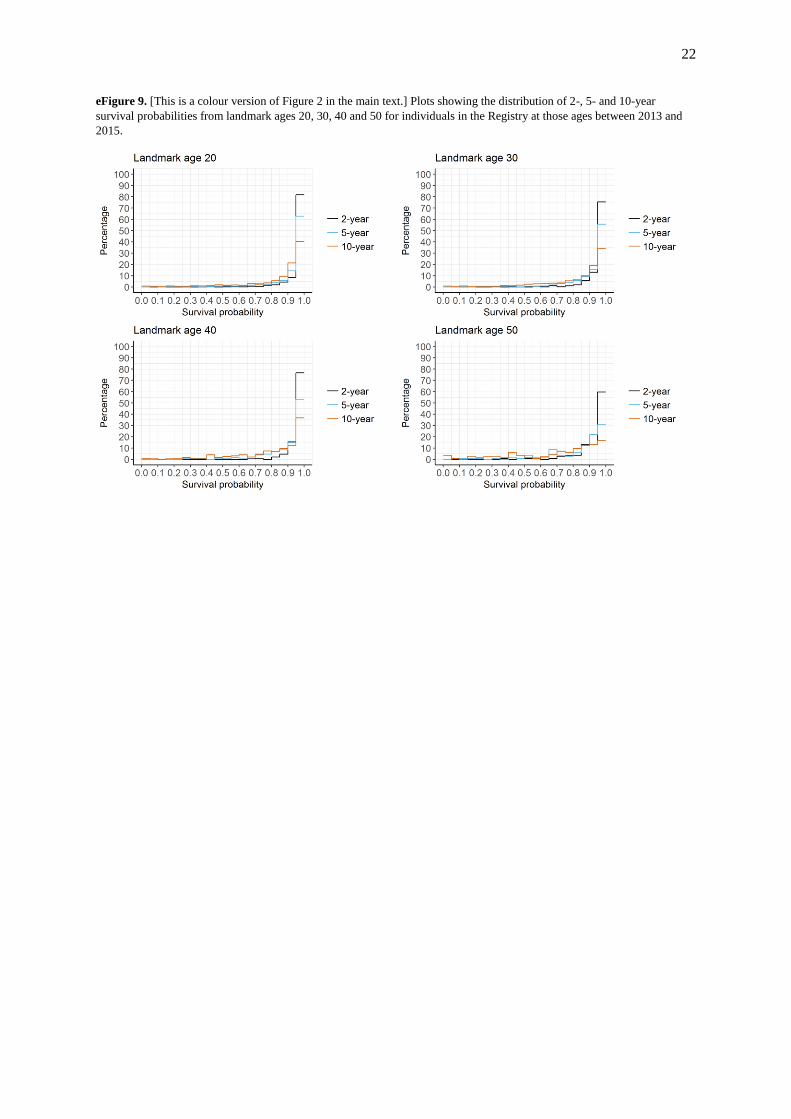
eFigure 9. [This is a colour version of Figure 2 in the main text.] Plots showing the distribution of 2-, 5- and 10-year
survival probabilities from landmark ages 20, 30, 40 and 50 for individuals in the Registry at those ages between 2013 and
2015.
23
References
1. Cox, D. R. Models and Life-Tables Regression. J. R. Stat. Soc. Ser. B. 34, 187–220 (1972).
2. Cox, D. R.. Partial likelihood. Biometrika 62, 269–276 (1975).
3. Breslow, N. Discussion of the paper by D. R. Cox. J. R. Stat. Soc. Ser. B 34, 216–217 (1972).
4. Yong, F., Cai, T., Wei, L. & Tian, L. Classical model selection. in Handbook of Survival
Analysis (eds. Klein, J., van Houwelingen, H., Ibrahim, J. & Scheike, T.) (CRC Press, 2014).
5. Pencina, M. J., D’Agostino, R. B., D’Agostino, R. B. & Vasan, R. S. Evaluating the added
predictive ability of a new marker: From area under the ROC curve to reclassification and
beyond. Stat. Med. 27, 157–172 (2008).
6. Uno, H., Cai, T., Pencina, M. J., D’Agostino, R. B. & Wei, L. J. On the C-statistics for
evaluating overall adequacy of risk prediction procedures with censored survival data. Stat.
Med. 30, 1105–1117 (2011).
7. Gerds, T. A., Kattan, M. W., Schumacher, M. & Yu, C. Estimating a time-dependent
concordance index for survival prediction models with covariate dependent censoring. Stat.
Med. 32, 2173–2184 (2013).
8. Antolini, L., Boracchi, P. & Biganzoli, E. A time-dependent discrimination index for survival
data. Stat. Med. 24, 3927–3944 (2005).
9. Graf, E., Schmoor, C., Sauerbrei, W. & Schumacher, M. Assessment and comparison of
prognostic classification schemes for survival data. Stat. Med. 18, 2529–2545 (1999).
10. Gerds, T. A. & Schumacher, M. Consistent Estimation of the Expected Brier Score in General
Survival Models with Right-Censored Event Times. Biometrical J. 48, 1029–1040 (2006).
11. van Houwelingen, H. C. & Putter, H. Dynamic prediction in clinical survival analysis. (CRC
Press/Chapman and Hall, 2012).
12. Kuhn, M. & Johnson, K. Over-Fitting and Model Tuning. In Applied Predictive Modelling. pp.
61–92 (Springer, 2013).
13. Therneau, T. A Package for Survival Analysis in S. R package version 2.38. https://CRAN.R-
project.org/package=survival (2015).
14. Putter, H. Dynpred package. https://cran.r-project.org/package=dynpred (2015).
15. Pinheiro, J., Bates, D., DebRoy, S., Sarkar, D. & R Core Team. nlme: Linear and Nonlinear
Mixed Effects Models. R package version 3.1-131.1. https://CRAN.R-
project.org/package=nlme (2018).
16. Nkam, L., Lambert, J., Latouche, A., Bellis, G., Burgel, P. R. & Hocine, M. N. A 3-year
prognostic score for adults with cystic fibrosis. J. Cyst. Fibros. 16, 701-708 (2017).
17. Liou, T. G., Adler, F.R., FitzSimmons, S. C., Cahill, B. C., Hibbs, J. R. & Marshall, B. C.
Predictive 5-year survivorship model of cystic fibrosis. Am. J. Epidemiol. 153, 345–352
(2001).
18. Mayer-Hamblett, N., Rosenfeld, M., Emerson, J., Goss, C. H. & Aitken, M. L. Developing
Cystic Fibrosis Lung Transplant Referral Criteria Using Predictors of 2-Year Mortality. Am. J.
Respir. Crit. Care Med. 166, 1550–1555 (2002).
19. McCarthy, C., Dimitrov, B. D., Meurling, I. J., Gunaratnam, C. & McElvaney, N. G. The CF-
ABLE score: A novel clinical prediction rule for prognosis in patients with cystic fibrosis.
Chest 143, 1358–1364 (2013).

24