supplementary materials for - california institute of...

advances.sciencemag.org/cgi/content/full/2/1/e1500989/DC1

Supplementary Materials for

An epidermis-driven mechanism positions and scales stem cell niches in

plants

Jérémy Gruel, Benoit Landrein, Paul Tarr, Christoph Schuster, Yassin Refahi, Arun Sampathkumar,

Olivier Hamant, Elliot M. Meyerowitz, Henrik Jönsson

Published 29 January 2016, Sci. Adv. 2, e1500989 (2016)

DOI: 10.1126/sciadv.1500989

This PDF file includes:

Fig. S1. Templates.

Fig. S2. Optimization strategy.

Fig. S3. The model is able to represent a large collection of perturbations.

Fig. S4. pCLV3::WUS.

Fig. S5. WUS domain size variation.

Fig. S6. CLV3 domain size variation.

Fig. S7. pCLV3 >> GFP meristem shapes and expression domains.

Fig. S8. clasp1 pWUS >> GFP meristems, grown in long days.

Fig. S9. clasp1 pWUS >> GFP meristems, grown in long days followed by short days.

Fig. S10. Col.0 pWUS >> GFP meristems, grown in long days.

Fig. S11. Col.0 pWUS >> GFP meristems, grown in long days followed by short days.

Fig. S12. WS-4 pWUS >> GFP meristems, grown in long days.

Fig. S13. WS-4 pWUS >> GFP meristems, grown in long days followed by short days.

Fig. S14. clasp1 pCLV3 >> GFP meristems, grown in long days.

Fig. S15. clasp1 pCLV3 >> GFP meristems, grown in long days followed by short days.

Fig. S16. Col.0 pCLV3 >> GFP meristems, grown in long days.

Fig. S17. Col.0 pCLV3 >> GFP meristems, grown in long days followed by short days.

Fig. S18. WS-4 pCLV3 >> GFP meristems, grown in long days.

Fig. S19. WS-4 pCLV3 >> GFP meristems, grown in long days followed by short days.

Fig. S20. Example of expression domain variations upon tissue shape changes.

Fig. S21. Meristem size measure versus shape measure.

Fig. S22. Long-range and short-range signals.

Fig. S23. WUS sensitivity analysis.

Fig. S24. CLV3 sensitivity analysis.

Table S1. Example parameter sets.

Legend for movie S1

Other Supplementary Material for this manuscript includes the following:

(available at advances.sciencemag.org/cgi/content/full/2/1/e1500989/DC1)

Movie S1 (.mp4 format). Primordium growth.

Figure S1 – Templates

The model runs on three different templates, from top to bottom, the lines display: the two-

dimensional abstract template, the three-dimensional abstract template and the realistic template.

From left to right and in green, are the fixed components used during computations: the boundaries

(L1 and Sink), the optimisation targets (WUS, CLV3 and KAN1), and the part of the template

considered during optimisation of tissues containing primordia.

Figure S2 - Optimization strategy The divide and conquer approach used to optimise the system is summed up in 5 steps. 1)

Optimisation of WUS using the template defined CLV3 expression domain. 2) Optimisation of

CLV3. 3) Re-optimisation of CLV3 peptide gradient. 4) Equilibrium of the core model. 5)

Optimisation of KAN1. Red: optimised elements, black: fixed element, blue: elements to stabilise,

grey: unused elements.

Figure S3 - The model is able to represent a large collection of perturbations

The top panel presents the wild type expression patterns obtained after optimisation and is compared

to the outcome of various perturbations of the system. Experimentally described mutants are

referenced in (12).

Figure S4 – pCLV3::WUS Comparison between wild type expression domains and a pCLV3::WUS mutant applied to a large

meristematic tissue

Figure S5 - WUS domain size variation

Comparison between size of WUS domains and size of SAMs for different growth conditions and

genotypes. LD indicates plants grown in long day conditions while SD-LD indicates plants grown

in short days followed by long days. A regression line is given with each plot along with its slope,

intercept and a p-value testing a null slope.

Figure S6 – CLV3 domain size variation

Comparison between size of CLV3 domains and size of SAMs for different growth conditions and

genotypes. LD indicates plants grown in long day conditions while SD-LD indicates plants grown

in short days followed by long days. A regression line is given with each plot along with its slope,

intercept and a p-value testing a null slope.

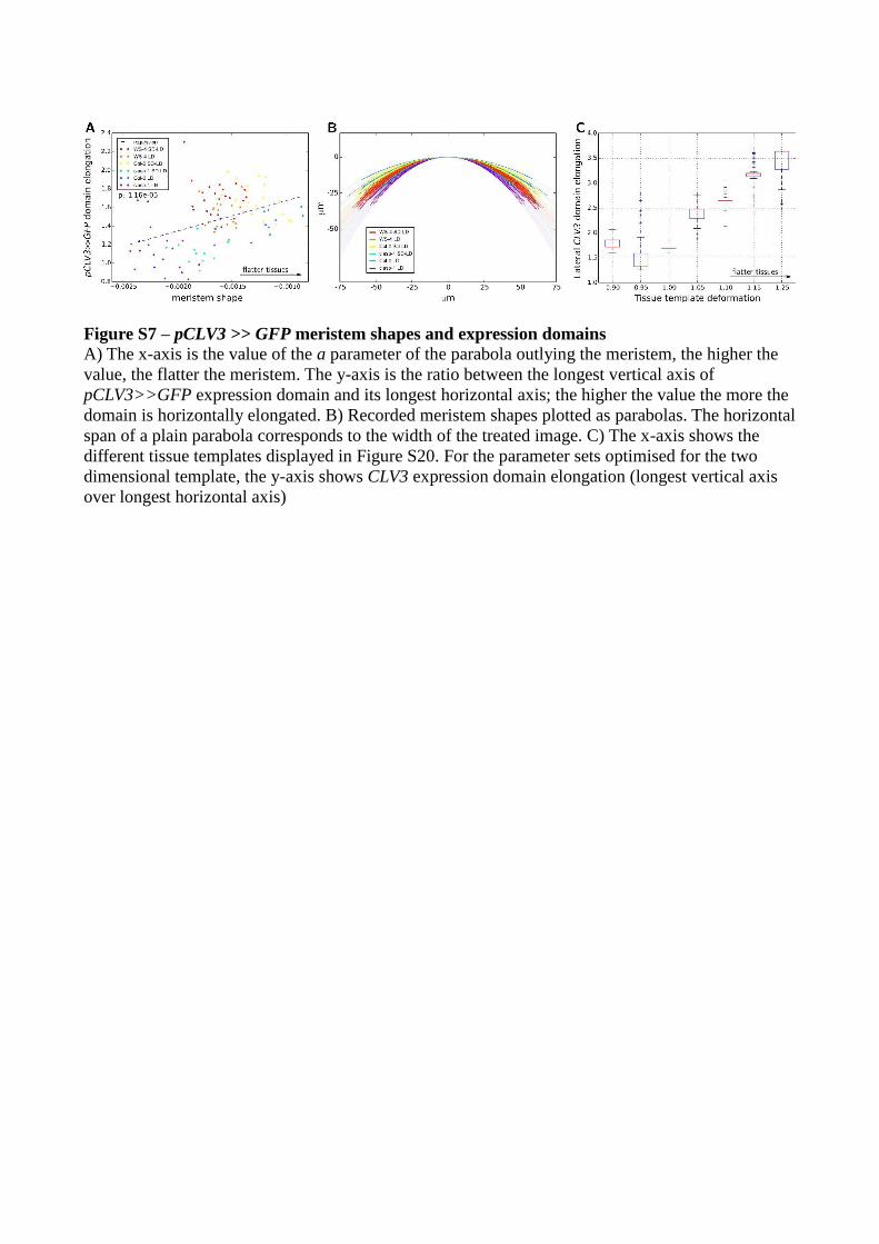
Figure S7 – pCLV3 >> GFP meristem shapes and expression domains

A) The x-axis is the value of the a parameter of the parabola outlying the meristem, the higher the

value, the flatter the meristem. The y-axis is the ratio between the longest vertical axis of

pCLV3>>GFP expression domain and its longest horizontal axis; the higher the value the more the

domain is horizontally elongated. B) Recorded meristem shapes plotted as parabolas. The horizontal

span of a plain parabola corresponds to the width of the treated image. C) The x-axis shows the

different tissue templates displayed in Figure S20. For the parameter sets optimised for the two

dimensional template, the y-axis shows CLV3 expression domain elongation (longest vertical axis

over longest horizontal axis)

Figure S8 - clasp1 pWUS >> GFP meristems, grown in long days

The top left number in each panel is the a parameter describing the blue parabola outlying the

meristem shape, the second number is the ratio of the two blue axis describing the expression

domain of WUS. The number above each meristem is a visual count of the amount of cell layers

between the tip of the meristem and the top of WUS expression domain. A few images were

manually corrected (blue patches) to help the algorithm quantifying the shape of the meristem and

expression domain. Scale bar: 20μm.

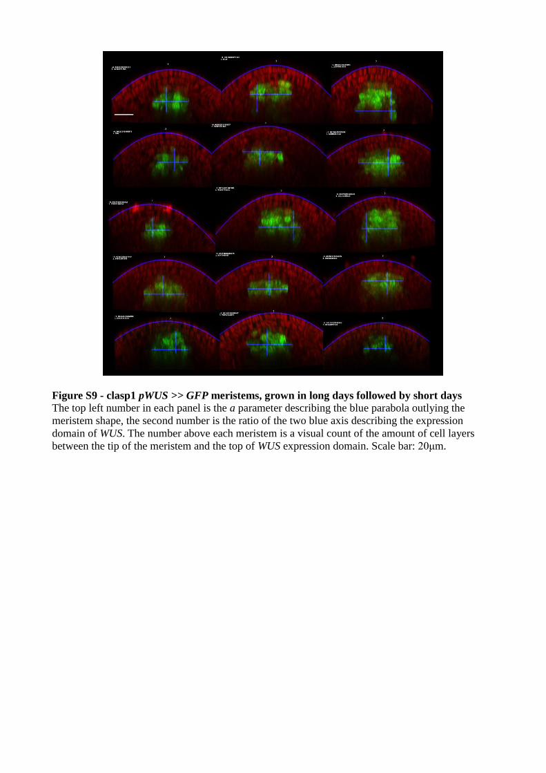
Figure S9 - clasp1 pWUS >> GFP meristems, grown in long days followed by short days




between the tip of the meristem and the top of WUS expression domain. Scale bar: 20μm.

Figure S10 – Col.0 pWUS >> GFP meristems, grown in long days





Figure S11 – Col.0 pWUS >> GFP meristems, grown in long days followed by short days




between the tip of the meristem and the top of WUS expression domain. In one image, the outline of

the meristem was manually traced (red line) to help the algorithm quantifying the shape. Scale bar:

20μm.

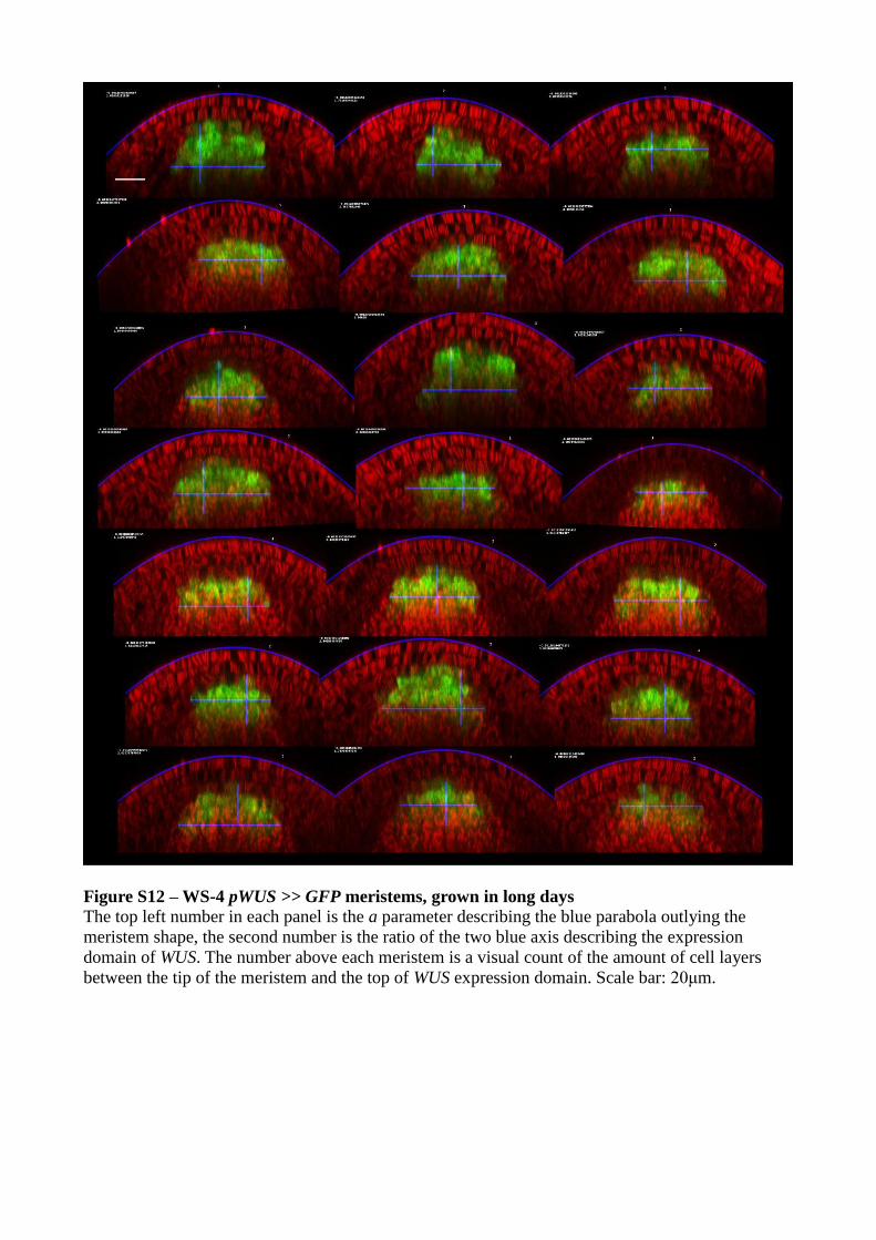
Figure S12 – WS-4 pWUS >> GFP meristems, grown in long days





Figure S13 – WS-4 pWUS >> GFP meristems, grown in long days followed by short days





Figure S14 - clasp1 pCLV3 >> GFP meristems, grown in long days



domain of WUS. Scale bar: 20μm.

Figure S15 - clasp1 pCLV3 >> GFP meristems, grown in long days followed by short days

The automatically defined parabolas and expression domain axes are displayed in blue. The top left

number in each panel is the a parameter describing the blue parabola outlying the meristem shape,

the second number is the ratio of the two blue axis describing the expression domain of WUS. Scale

bar: 20μm.

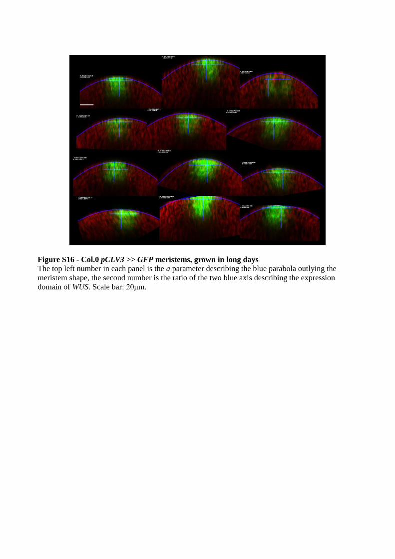
Figure S16 - Col.0 pCLV3 >> GFP meristems, grown in long days




Figure S17 - Col.0 pCLV3 >> GFP meristems, grown in long days followed by short days




Figure S18 - WS-4 pCLV3 >> GFP meristems, grown in long days




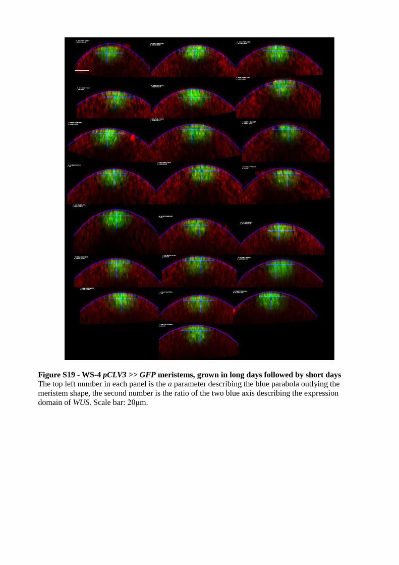
Figure S19 - WS-4 pCLV3 >> GFP meristems, grown in long days followed by short days




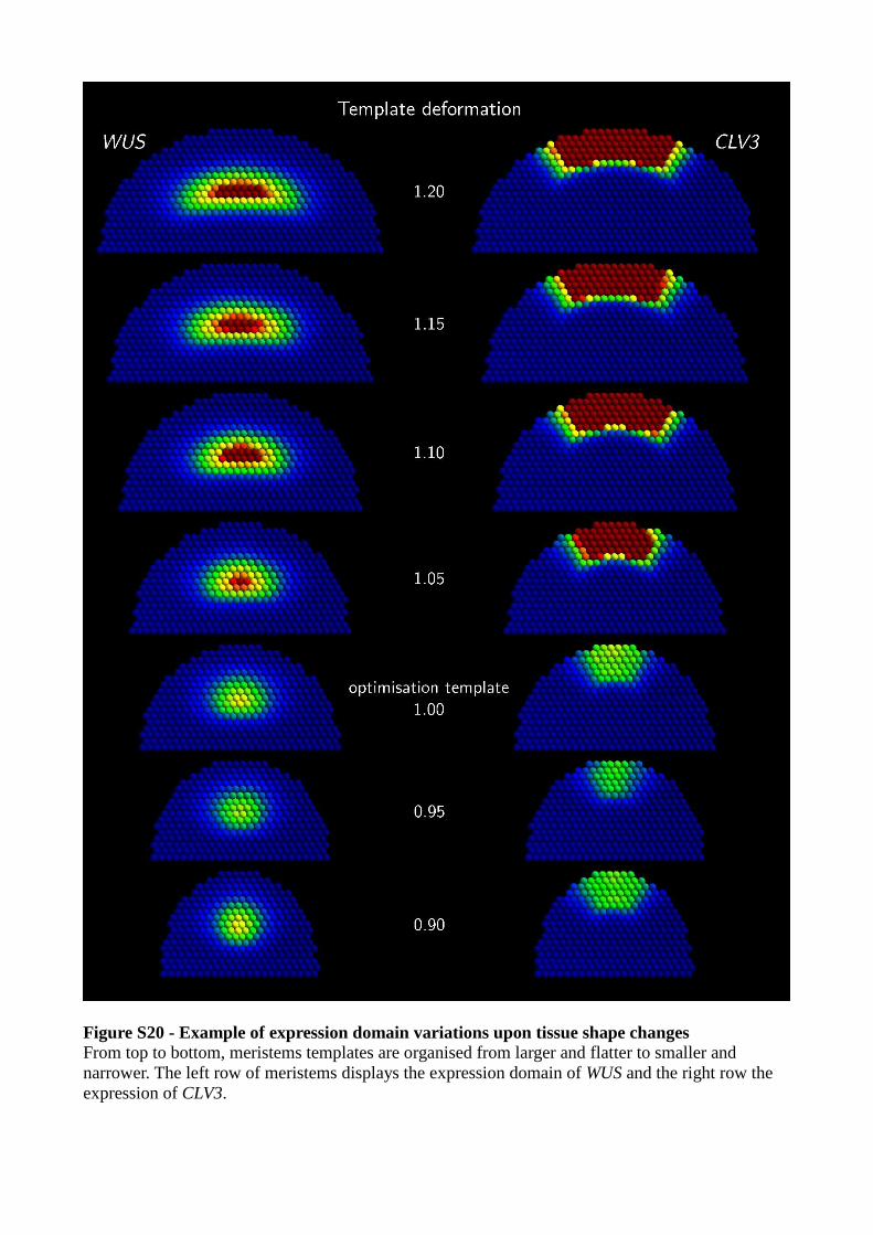
Figure S20 - Example of expression domain variations upon tissue shape changes

From top to bottom, meristems templates are organised from larger and flatter to smaller and

narrower. The left row of meristems displays the expression domain of WUS and the right row the

expression of CLV3.

Figure S21 - Meristem size measure versus shape measure

For both panels, the x-axis is the shape of the recorded parabolas (a parameter) for the measured

meristems. The y-axis is the measured meristem size (Figure 2, main text). In each panel, the linear

regression of the data is plotted and the resulting p-value indicated. A) pWUS>>GFP meristems. B)

pCLV3>>GFP meristems.

Figure S22 - Long-range and short-range signals

The two first panels plot the optimised diffusion rates against the optimised degradation rates

obtained for the three dimensional abstract (left) and realistic (right) templates. The top two dashed

lines represent the short-range signals exemplified in Figure 5 (main text), the bottom one is the

long-range signal. The right panel explains the outlier point of the realistic template panel (blue

point at the bottom) where CLV3a has a long-range type of signal. The simulation presents the

outcome of a pCLV3::WUS mutant in the case of the outlier and in another example. The outlier can

be rejected as it does not display the correct overlap of both WUS and CLV3 domains in the outer

cell layers.

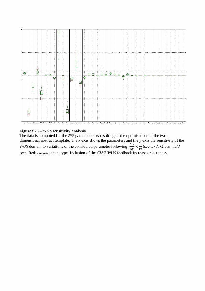
Figure S23 – WUS sensitivity analysis

The data is computed for the 255 parameter sets resulting of the optimisations of the two-

dimensional abstract template. The x-axis shows the parameters and the y-axis the sensitivity of the

WUS domain to variations of the considered parameter following: Δ𝑚

Δ𝑝×

𝑝

𝑚 (see text). Green: wild

type. Red: clavata phenotype. Inclusion of the CLV3/WUS feedback increases robustness.

Figure S24 – CLV3 sensitivity analysis

The data is computed for the 255 parameter sets resulting of the optimisations of the two-

dimensional abstract template. The x-axis shows the parameters and the y-axis the sensitivity of the

CLV3 domain to variations of the considered parameter following: Δ𝑚

Δ𝑝×

𝑝

𝑚 (see text). Green: wild

type. Red: clavata phenotype. Inclusion of the CLV3/WUS feedback increases robustness.

parameter 2D 3D Real parameter 2D 3D Real

𝑉𝑊 8.42e+00 1.84e+01 1.51e+01 𝑘𝐿𝑐𝑊 1.13e+01 8.20e+00 1.79e+01

𝑛𝐿𝑐𝑊 1.04e+01 2.09e+01 7.26e+00 𝑘𝐿𝑎𝑊 2.19e+01 1.00e-04 7.99e+00

𝑛𝐿𝑎𝑊 1.62e+00 1.34e+00 1.99e+00 𝑘𝑐𝑊 1.24e+01 6.67e+00 5.07e-02

𝑛𝑐𝑊 1.00e+00 1.00e+00 6.66e+00 𝑔𝑊 6.05e-03 2.39e-04 2.29e-03

𝑝𝑤 1.68e+01 1.03e+01 1.50e+00 𝑔𝑤 1.49e+00 1.37e+01 2.10e-13

𝐷𝑤 1.21e+01 2.07e+01 4.37e+00 𝑉𝐶 3.84e+01 1.24e+01 1.80e+01

𝑘𝐿𝐶𝐶 1.36e+00 6.10e+00 3.08e+00 𝑛𝐿𝐶𝐶 1.77e+00 1.51e+01 9.20e+00

𝑘𝑤𝐶 2.97e+00 8.21e-02 3.94e+00 𝑛𝑤𝐶 9.52e+00 3.63e+00 5.36e+00

𝑔𝐶 1.69e-02 5.59e-02 3.76e+00 𝑝𝑐 4.39e+00 2.27e+00 3.97e+00

𝑔𝑐 7.61E-02 3.46e-15 1.02e+01 𝐷𝑐 2.71e+00 4.63e+00 3.45e-12

𝑉𝐾 7.74e+00 2.00e+00 𝑘𝐿𝐾𝐾 1.76e+01 5.85e-01

𝑛𝐿𝐾𝐾 1.33+00 1.43e+00 𝑘𝑤𝐾 5.39e-01 9.63e-03

𝑛𝑤𝐾 4.47e+00 4.10e+00 𝑔𝐾 6.78e+00 1.97e+00

𝑝𝐿𝑐 1.10e+00 2.21e+01 3.28e+00 𝑔𝐿𝑐 2.63e-06 8.38e-02 5.97e-04

𝐷𝐿𝑐 1.04e+00 1.57e+01 4.90e+00 𝑝𝐿𝑎 1.45e+00 2.41e+00 5.76e+00

𝑔𝐿𝑎 3.45e-05 2.70e-01 1.80e-03 𝐷𝐿𝑎 3.00e-05 2.45e-02 4.51e-03

𝑝𝐿𝐶 1.37e+01 5.23e+00 4.65e-01 𝑔𝐿𝐶 2.83e+00 1.00e-04 3.11e-13

𝐷𝐿𝐶 1.10e+00 7.57e+00 3.43e+00 𝑝𝐿𝐾 1.14e+01 2.61e+01

𝑔𝐿𝐾 1.76e-04 3.48e-02 𝐷𝐿𝐾 5.07e-08 1.00e-04

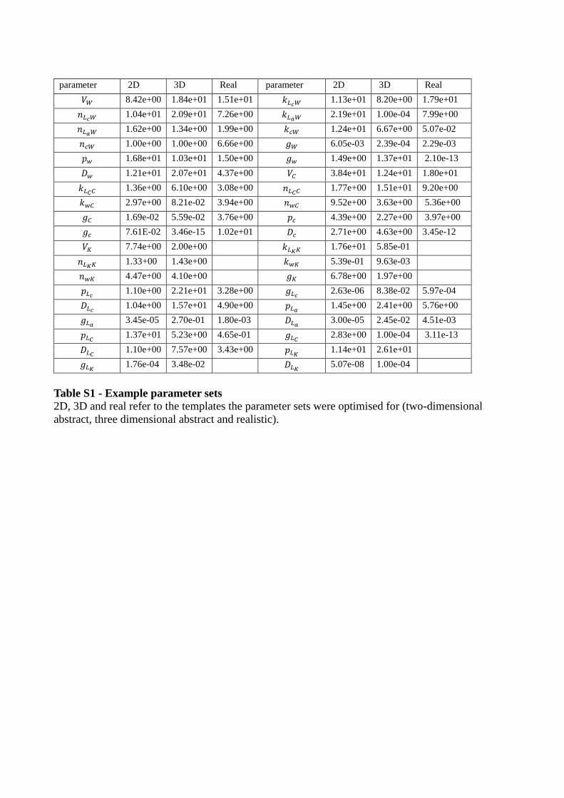
Table S1 - Example parameter sets

2D, 3D and real refer to the templates the parameter sets were optimised for (two-dimensional

abstract, three dimensional abstract and realistic).

Movie S1 - Primordium growth

Simulation showing the result of the growth of a primordium like domain on the side of the three-

dimensional abstract template. The colour scale for gene expression domains is the same as in

Figure 1. The colour scale for diffusing molecules is relative to the concentration of the considered

molecule across the whole simulation (red: maximum, blue: minimum).

supplementary materials for - california institute of...

Documents