supplementary material: probabilistic cause-of-death ...tylermc/insilico_supplement_r1.pdf ·...

Supplementary Material: Probabilistic Cause-of-death Assignment

using Verbal Autopsies∗

Tyler H. McCormick1,2,3,*, Zehang Richard Li1, Clara Calvert8,6, Mia Crampin6,8,9,Kathleen Kahn5,7, and Samuel J. Clark3,4,5,6,7

1Department of Statistics, University of Washington2Center for Statistics and the Social Sciences (CSSS), University of Washington

3Department of Sociology, University of Washington4Institute of Behavioral Science (IBS), University of Colorado at Boulder

5MRC/Wits Rural Public Health and Health Transitions Research Unit (Agincourt), School of PublicHealth, Faculty of Health Sciences, University of the Witwatersrand

6ALPHA Network, London7INDEPTH Network, Ghana

8London School of Hygiene and Tropical Medicine9Karonga HDSS, Malawi

*Correspondence to: [email protected]

1 Simulation studies

To evaluate the potential of InSilicoVA and to compare it to InterVA, we fit both InSilicoVA andInterVA to simulated data and compare the results in terms of accuracy of individual cause as-signment. We performed two simulation studies using data generated with various conditionalprobability matrices Ps|c designed to explore different aspects of the performance of the two mod-els, and within each study we compared three levels of additional variation to reflect conditionscommonly found in practice.

In each case we simulated 100 datasets, each with 1, 000 deaths. For each dataset we firstsimulated a set of deaths with a pre-specified cause distribution. Since cause distributions varysubstantially between areas, we used the reported population cause distribution from multipleHDSS sites in the ALPHA network (Maher et al., 2010), mentioned in the introduction. Foreach simulation run, we randomly picked the Agincourt study, uMkhanyakude cohort, or KarongaPrevention Study/Kisesa open cohort HDSS site, then used the cause distribution from that siteas the “true” cause distribution in that simulation run. Karonga and Kisesa actually representtwo HDSS sites, though we combined their results for our simulation purposes because both haverelatively small sample sizes.

∗Preparation of this manuscript was supported by the Bill and Melinda Gates Foundation, with partial supportfrom a seed grant from the Center for the Studies of Demography and Ecology at the University of Washingtonalong with grant K01 HD057246 to Clark and K01 HD078452 to McCormick, both from the National Institute ofChild Health and Human Development (NICHD). The authors are grateful to Peter Byass, Basia Zaba, Laina Mercer,Stephen Tollman, Adrian Raftery, Philip Setel, Osman Sankoh, and Jon Wakefield for helpful discussions. We are alsograteful to the MRC/Wits Rural Public Health and Health Transitions Research Unit and the Karonga PreventionStudy for sharing their data for this project.

1

In the simulation studies that follow we explore various aspects of the performance of InSili-coVA and InterVA. Recall that we wish to assign causes of death and estimate a population causedistribution using data from the VA interviews and the physician-reported cause – sign/symptomassociation matrix Ps|c. We focus specifically on the first two limitations we identified with InterVA:lack of a probabilistic framework and inability to quantify uncertainty. In Section 1.1 we evaluateminor/no perturbation to Ps|c under more realistic scenarios in which data from VA interviewsare missing or imperfect. Then in Section 1.2 we examine the performance of both models whenaltering the range of possible probabilities in Ps|c. These simulations demonstrate that the choice ofvalues of Ps|c impacts the resulting cause assignments and population cause distribution, providingevidence and support for our probabilistic approach that appropriately captures this uncertainty.

1.1 Simulation 1: InterVA Ps|c

The first set of three simulation studies maintains the basic structure of the table of conditionalprobabilities Ps|c that describes the associations between signs/symptoms and causes. Three varia-tions explore the ideal situation, the effect of changing the precise values in Ps|c and what happenswhen the data are not perfect.

Baseline First we test and compare InSilicoVA and InterVA under “best case” conditions inwhich both use perfect information. To accomplish this we use the association between signs/symptomsand causes described in Table 1 in the paper. In each simulation run we sample a new conditionalprobability matrix Ps|c with exactly the same distribution of levels as displayed in Table 1 from thepaper. In this setup both InSilicoVA and InterVA are given the sampled Ps|c so that they have thetrue conditional probability matrix used to simulate symptoms, i.e. they have all the informationnecessary to recover the “real” individual cause assignments. For InsilicoVA this means that theprior mean of the conditional probability matrix is correct, and InterVA has correct conditionalprobabilities. We run both algorithms on the simulated data. For InSilicoVA the cause assignedto each death is the one with the highest posterior mean, and for InterVA the assigned cause isthe one with the highest final propensity score. Accuracy is the fraction of simulated deaths withassigned causes matching the simulated cause.

The left panel of Figure 1 displays accuracy of both methods. We also computed accuracy forthe top three causes for each method and found only very minor differences in the results. Underthese ideal conditions InsilicoVA performs nearly perfectly all the time, and InterVA also performswell, although there is more variance in the performance of InterVA.

Resampled Ps|c Next we test the effect of mis-specifying the exact numeric values of Ps|c, asituation that is always true in reality. It is not realistic to expect physicians to produce numericallyaccurate conditional probabilities associating causes with signs/symptoms, and for this reasonwe want to understand the extent to which each method is affected by mis-specification of theconditional probability values in Table 1 in the main paper. Recall that the Ps|c supplied withInterVA (described in Table 1 from the manuscript and used throughout this paper) contains theranked lists of signs/symptoms provided by physicians and arbitrary values attached to each level.

We performed a simulation designed to evaluate the sensitivity of the algorithms to the valuesassigned to the conditional probabilities in Ps|c. The probabilities assigned by InterVA increaseapproximately linearly on a log scale. We preserve this relationship but assign new values to eachprobability in Ps|c by drawing new values uniformly between log(10−6) and log(0.9999) and thenexponentiating and ordering the results. We fit both methods with the new Ps|c on the simulateddata described above.

2

Figure 1: Simulation setup 1: InterVA Ps|c.

●●●

●

●

●●

0.0

0.2

0.4

0.6

0.8

1.0

Baseline

Acc

urac

y

InsilicoVA InterVA

●●●●●●●

●●

●

●●●

●

0.0

0.2

0.4

0.6

0.8

1.0

Resampled

Acc

urac

y

InsilicoVA InterVA

●●

●

●

●

●

●

0.0

0.2

0.4

0.6

0.8

1.0

Reporting Error

Acc

urac

y

InsilicoVA InterVA

Both InSilicoVA and InterVA use the Ps|c supplied by InterVA. Left: Classification accuracy of deaths by causeusing ideal simulated data, i.e. data generated directly from Ps|c with no alteration. Middle: Classificationaccuracy when using resampled Ps|c. Right: Classification accuracy when there is 10% reporting error.

The middle panel of Figure 1 displays the accuracy of both methods using the misspecified Ps|con the ideal simulated data. InSilicoVA’s performance is unchanged indicating that InSilicoVA isable to adjust the probabilities correctly using the data and is therefore more robust to misspec-ification of the conditional probability table. InterVA performs slightly worse with a reduction inmedian accuracy and an increase in accuracy variance.

Reporting Error Finally we investigate the effects of reporting error. Given the nature of VAquestionnaires we expect multiple sources of error in the data. To explore the impact of reportingerror like this, we conduct a third simulation that includes reporting error. We first generate dataas described above for the best case baseline simulation; then we randomly choose a small fractionof signs/symptoms and reverse their simulated value, i.e. generate some false positive and falsenegative reports of signs/symptoms.

The accuracy of each method run on simulated data with reporting error is contained in theright panel of Figure 1. Reporting error reduces the accuracy and increases the variance in accuracyfor both methods. The effect on InSilicoVA is relatively small with median accuracy pulled downto ∼ 95%, while InterVA suffers dramatically with a median accuracy of less than 40% and a largeincrease in accuracy variance.

1.2 Simulation 2: Compressed range of values in Ps|c

The second set of simulation studies investigates the performance of the two methods with amodified set of conditional probabilities Ps|c. The Ps|c supplied with InterVA contains very ex-treme values that range from [0, 1] inclusive. The extreme values in this table give their cor-responding signs/symptoms disproportionate influence that can overwhelm any/all of the othersigns/symptoms occurring with a death. This set of simulation studies is aimed at understandingthe effect of the extreme values in Ps|c. To accomplish this we retain the log-linear relationship

3

among the ordered values in Ps|c, but we draw new values for each of the conditional probabilitiesfrom the range [0.25, 0.75]. We then repeat the same three simulation studies described above.The results are shown in Figure 2. This change significantly degrades the performance of both

Figure 2: Simulation setup 2: compressed range of values in Ps|c.

●●

●

●

0.0

0.2

0.4

0.6

0.8

1.0

Baseline

Acc

urac

y

InsilicoVA InterVA

●●

●

0.0

0.2

0.4

0.6

0.8

1.0

Resampled

Acc

urac

y

InsilicoVA InterVA

0.0

0.2

0.4

0.6

0.8

1.0

Reporting Error

Acc

urac

y

InsilicoVA InterVA

Both InSilicoVA and InterVA use new Ps|c with values restricted to the range [0.25, 0.75]. Left:Classification accuracy of deaths by cause using ideal simulated data, i.e. data generated directlyfrom Ps|c with no alteration. Middle: Classification accuracy when using resampled Ps|c. Right:Classification accuracy when there is 10% reporting error.

InSilicoVA and InterVA with reductions in median accuracy and increases in accuracy variance.Yet across all scenarios InsilicoVA still maintains a mean performance around 70 − 90% while In-terVA drops to around 40−60% with larger variance. Given this substantial reduction in accuracy,we also calculate accuracy using the top three causes identified by each method. In practice it isstill useful to have the correct cause identified as one of the top three. Figure 3 displays accuracyallowing any of the three most likely causes to agree with the true cause. Accuracy increases forboth algorithms, but InsilicoVA consistently outperforms InterVA by more than 10% and withmuch smaller variance. This result indicates that InterVA relies on the extreme values in Ps|c whileInsilicoVA is more robust in situations where the conditional probabilities are less informative.

2 PHMRC data summary

In this section we describe the PHMRC data in additional detail. We also describe in detail theother methods we use for comparison and provide specifics about our evaluation metrics.

2.1 Original data

The data consist of 7, 841 adult deaths collected in Murray et al. (2011b) from six sites (see Table 1).Each death in the raw format consist of 251 items and 678 stem word indicators from free text inthe interviewer’s recording. The gold standard causes are provided in three levels each consistingof 55, 46 and 34 causes. We use the highest level cause list with 34 causes.

4

Figure 3: Simulation setup 2, top 3: compressed range of values in Ps|c.

●

●

●

●

●

●

●●●

0.0

0.2

0.4

0.6

0.8

1.0

Baseline

Top

3 A

ccur

acy

InsilicoVA InterVA

●

●●

●

●

●

●

●

●

0.0

0.2

0.4

0.6

0.8

1.0

Resampled

Top

3 A

ccur

acy

InsilicoVA InterVA

●

0.0

0.2

0.4

0.6

0.8

1.0

Reporting Error

Top

3 A

ccur

acy

InsilicoVA InterVA

Both InSilicoVA and InterVA use new Ps|c with values restricted to the range [0.25, 0.75]. Accuracycalculated using the three most likely causes identified by each method; if the correct cause is one ofthe top 3, the death is considered to be accurately classified. Left: Classification accuracy of deaths bycause using ideal simulated data, i.e. data generated directly from Ps|c with no alteration. Middle:Classification accuracy when using resampled Ps|c. Right: Classification accuracy when there is 10%reporting error.

Table 1: Sample size in each of the six sites.

AP Bohol Dar Mexico Pemba UP

Size 1554 1259 1726 1586 297 1419

2.2 Selected symptoms

2.2.1 Items

We extracted 164 items corresponding to symptoms and demographics information (sex, age, drink-ing, etc.) out of the 251 (the rest are designated as about the health care experience and informationabout the interviewee). For each item we convert the response into three categories: Yes (“Y”),No (“N”), and Missing (“.”), where missing includes “Don’t Know”, “Refused to Answer” and nodata. After dichotomization, we have 177 items.

To dichotomize the variables into these three categories, we followed the following two rules:

1. Continuous variables Use a cut-off value to decide if it is short/small or long/large. Thecut-off used are in Additional file 9 provided in Murray et al. (2011b)

2. Categorical variables with multiple levels Split into multiple questions or combine somelevels based on Additional file 10 provided in Murray et al. (2011b)

2.2.2 Words

The words came from two sources: (1) questions such as “Where was the rash located?: face,trunk, extremities, everywhere, or other (specify: ).” and (2) open-ended section at the end of

5

questionnaire. In the original paper (Murray et al., 2011b), they further mapped the 678 keywordsinto 106 binary variables as a word dictionary (See Additional file 12 provided in Murray et al.(2011b)).

For the words in the first case, we simply added an “other” category in the dichotomizationprocess described above. We grouped all responses not in the specified categories into “other”, andtreat it as a level in the categorical variables.

Words in the second case are referred to as Healthcare Experience (HCE) by Murray et al.(2011b). There are two sources of HCE in the data: (1) questions similar to “Have you ever beendiagnosed with...” and (2) free text parsed and stemmed from open-ended section. HCE has beenreported to significantly increase algorithm performance. yet to achieve fair comparison with theother methods, we exclude all HCE information in the comparison.

2.2.3 Comments on selected symptoms

There are some undocumented symptoms in the data.

• There are some repeated questions with different questions, e.g. a2 63 1 and a2 63 2. In suchsituations, both are included.

• The age of the deceased is recorded in two items, g1 07 and g5 04, and usually slightlydifferent. We used g1 07 only.

2.3 Simulation approaches

To evaluate the performances of different methods, we conducted three studies where the data isdivided into train and test set in the following three ways:

• Randomly assign 75% of deaths as training set and use the rest of the data as testing set.Repeat the steps and do analysis 100 times.

• Randomly assign 75% of deaths as training set. Sample a CSMF distribution fromDirichlet(1),and resample the rest of the data to match the generated CSMF. Use this re-sampled datasetas testing set. Further information on this approach below.Repeat the steps and do analysis100 times.

• Each time extract one site as testing set, and use the following three types of training set:

– all the data as training set,

– all the rest of the data as training set,

– one of the sites as training set.

Implementation of train-test split in literature All three papers from IHME (James et al.(2011), Murray et al. (2011b) and Murray et al. (2014)) use the same train-test split procedure:

1. Split the data with N death into 75% training and 25% testing.

2. Sample a CSMF distribution from noninformative Dirichlet. The above papers do not specifywhat “noninformative” means precisely. We assume it means Dirichlet(1).

3. Re-sample within test set with replacement, to create a new set with N death and CSMF assampled in previous step.

4. Repeat the steps and do analysis 500 times.

6

2.4 Comparison methods

We now present detailed descriptions of the methods used for comparison on the PHMRC data.

2.4.1 Tariff (James et al., 2011)

Let Xij denotes the count of combination for cause i and symptom j. Tariff score calculates

Tariffij =Xij −median(X1j , X2j , ..., XCj)

IQR(X1j , X2j , ..., XCj)

Then Tariff score for each death n = 1, 2, ..., N and cause i = 1, 2, ..., C is calculated by

Scoreni =

S∑j=1

Tariffij1nj

where 1nj denotes the indicator for symptom j exists in death i.A few implementation details in the paper:

1. Tariffij is rounded to the closest 0.5, which the authors claim is to avoid over-fitting.

2. For each cause (row) of Tariffij , only the top 40 values are used, others are forced to be 0.The referenced paper does not explicitly say top 40 in terms of absolute value, though this isour best deduction based on the information available.

Tariff score into rank This deals with how to assign cause of death given a vector of tariff scorefor each death. The easiest way is to just assign the cause based on score values. Desai et al. (2014)reported the simple approach performs better.

The method to turn Tariff score into ranks is described as

1. Re-sample training set to have uniform cause distribution. Maybe it means stratified re-sampling training set so all causes have the same counts?

2. In the re-sampled training set, calculates Tariff score for each death.

3. The distribution of Tariff score under each cause obtained are taken to be a reference distri-bution to calculate ranks from.

Based on the description in the published work, we are unclear about the number of re-samplingiterations for the training set. The description of the “uniform cause distribution” is also notsufficiently precise for replication. We have attempted to follow the published description as closelyas possible.

Updated methods (Murray et al., 2014) This is some update of Tariff method since firstintroduced. The major changes are as follows:

1. 500 bootstrapped samples of symptom data were used to recreate the tariff matrix.

2. Constraints were added to disallow biologically impossible cause of death assignments.

3. When changing score into rank, if the highest rank is not high enough (for example, 89%percentile for adults), it will be classified as “undetermined”.

7

Based on the brief descriptions in the Tariff update, we are able to follow the first change ofbootstrap. The second change requires detailed instruction to remove impossible causes and thusimpossible to replicate. To ensure fair comparisons with other methods, we do not assume anyundetermined causes throughout the analysis.

Open-sourced Tariff Method Desai et al. (2014) citetdesai2014performance used open-sourced Tariff method they developed, without specifying the test-train split detail. As accordingto the additional file 1 of the paper, the method is freely available at www.cghr.org/. We wereunable to find the codes for the method on this website. They use a symptom set of 96 indicators,but they did not specify the details of the indicators.

Our implementation For our implementation, we basically followed the original Tariff methodwith minor update. We use all the tariff instead of only top 40 values. In practice we found thisgives better accuracy. The tariff matrix contains only significant cells after bootstrapping 100 timesas suggested by the updated Tariff. And we performed the rank transform as discussed above. Wefound the rank transformed Tariff score to be always more accurate than the original scores, whichis consistent with the findings in James et al. (2011) but different from Desai et al. (2014).

2.4.2 King-Lu implementation (King and Lu, 2008)

The basic formulation of King-Lu method is

Pr(S) = Pr(S|C)train Pr(C),

where S indicates random sample of a subset of k symptoms, and the Pr(S) is estimated by both

training and testing data. The assumption for the above equation to hold is Pr(S|C)train =Pr(S|C)test. The CSMF of interest is Pr(C), which is estimated by constrained least square, andaveraged across different draws of S.

We used the R package VA provided on the authors’ website, though we note that this packageis no longer compatible with the latest versions of R. We set the number of subset symptoms to be10. Higher number of subset is recommended by the authors in cases where the number of totalsymptoms is high. But it gets less stable in our experiment.

2.4.3 SSP implementation (Murray et al., 2011a)

We implemented Simplified Symptom Pattern method as proposed in Murray et al. (2007). Thecore algorithm calculates

P (C|~S) =P (~S|C)P (C)∑′C P (~S|C ′)P (C ′)

,

where P (C) are calculated from King-Lu algorithm, and the subset of symptoms ~S are simplerandom draws of 15 symptoms from the whole set. The P (C|~S) are calculated by taking the meanof repeated draws of symptoms. We performed 50 draws as in the original paper.

2.4.4 InterVA implementation (Byass et al., 2012)

In both InterVA and InsilicoVA implementation, we need to extract a conditional probability tablefrom the training data. We first remove all symptoms that are missing over 95% of the times, andthen calculate the empirical conditional probability of symptoms given each cause. Then we need

8

www.cghr.org/

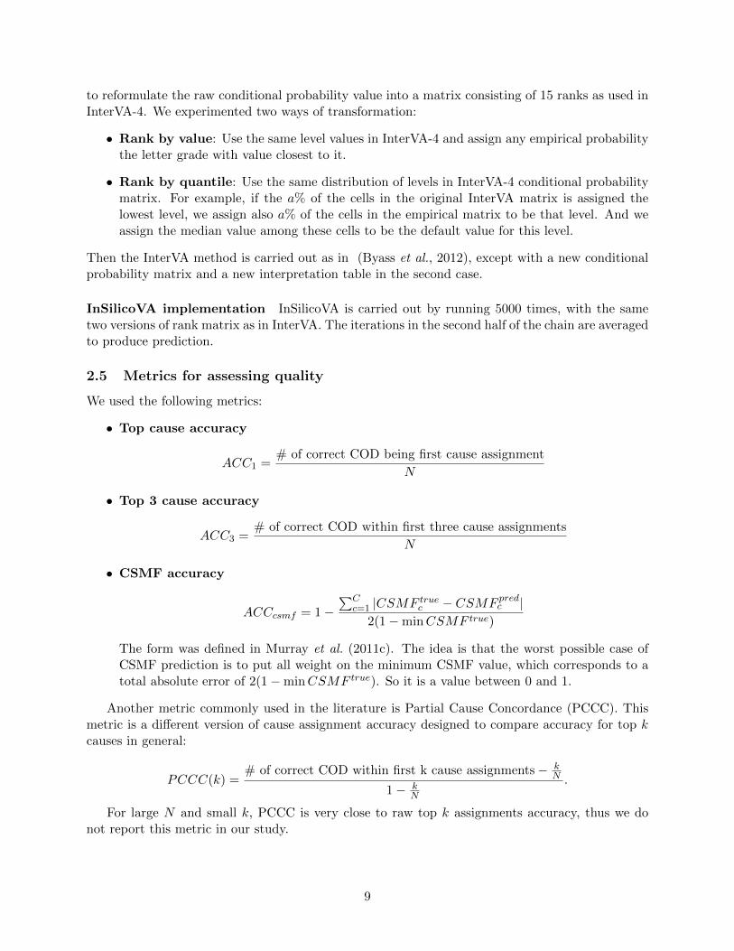
to reformulate the raw conditional probability value into a matrix consisting of 15 ranks as used inInterVA-4. We experimented two ways of transformation:

• Rank by value: Use the same level values in InterVA-4 and assign any empirical probabilitythe letter grade with value closest to it.

• Rank by quantile: Use the same distribution of levels in InterVA-4 conditional probabilitymatrix. For example, if the a% of the cells in the original InterVA matrix is assigned thelowest level, we assign also a% of the cells in the empirical matrix to be that level. And weassign the median value among these cells to be the default value for this level.

Then the InterVA method is carried out as in (Byass et al., 2012), except with a new conditionalprobability matrix and a new interpretation table in the second case.

InSilicoVA implementation InSilicoVA is carried out by running 5000 times, with the sametwo versions of rank matrix as in InterVA. The iterations in the second half of the chain are averagedto produce prediction.

2.5 Metrics for assessing quality

We used the following metrics:

• Top cause accuracy

ACC1 =# of correct COD being first cause assignment

N

• Top 3 cause accuracy

ACC3 =# of correct COD within first three cause assignments

N

• CSMF accuracy

ACCcsmf = 1−∑C

c=1 |CSMF truec − CSMF predc |2(1−minCSMF true)

The form was defined in Murray et al. (2011c). The idea is that the worst possible case ofCSMF prediction is to put all weight on the minimum CSMF value, which corresponds to atotal absolute error of 2(1−minCSMF true). So it is a value between 0 and 1.

Another metric commonly used in the literature is Partial Cause Concordance (PCCC). Thismetric is a different version of cause assignment accuracy designed to compare accuracy for top kcauses in general:

PCCC(k) =# of correct COD within first k cause assignments− k

N

1− kN

.

For large N and small k, PCCC is very close to raw top k assignments accuracy, thus we donot report this metric in our study.

9

2.6 Results using CCC

For comparability with existing literature, we also evaluated our method using chance-correctedconcordance. This metric can be defined as follows:

• chance-corrected concordance (CCC) for cause j

CCCj =

TPj

TPj+TNj− 1

N

1− 1N

where TPj is the number of true positive for cause j, and TNj is the number of true negativefor cause j. It is worth noting particularly here that the definition of TNj is the the numberof cases where cause assigned to a death is not cause j while the true cause is cause j.

So CCC could also be written as

CCCj =

# correctly assigned to cause j# total number of death from cause j −

1N

1− 1N

.

• overall chance-corrected concordance (CCC) Then the overall CCC is defined as a weightedsum of cause-specific CCC. Three ways to construct the weight is discussed in Murray et al.(2011c), and “based on considerations of simplicity of explanation, ease of implementation,and comparability”, they recommend the overall CCC be calculated as the average of thecause-specific CCC, i.e., equal weights will be used.

Using this metric, Figures 4 show results from the same evaluation study presented in the mainpaper. As in the main paper, the left panel in Figure 4 has results for the case where we samplea simple random sample without replacement for testing/training causes and the right panel inFigure 4 uses the Dirichlet procedure described above.

Figure 4: Random and Dirichlet sample CCC results

●

●●●●

0.2

0.3

0.4

InSilic

oVA

Quant

ile p

rior

InSilic

oVA

Table

1 p

rior

Inte

rVA

Quant

ile p

rior

Inte

rVA

Table

1 p

rior Ta

riff

SSP

Method

CC

C

Chance−corrected concordance100 random train−test splits

●

●

●●●●●

●

0.2

0.3

0.4

InSilic

oVA

Quant

ile p

rior

InSilic

oVA

Table

1 p

rior

Inte

rVA

Quant

ile p

rior

Inte

rVA

Table

1 p

rior Ta

riff

SSP

Method

CC

C

Chance−corrected concordance100 random splits with re−sampling

10

3 Results for cross-site comparisons

In this section we provide additional results obtained by using each site in the PHMRC dataas testing data, then using as training set: (1) all the sites, (2) all other sites, and (3) - (8)each of the single sites. These results indicate that performance is very sensitive to the modelinputs, i.e., the training set. For each site, we present results of (1) CCC, (2) CSMF accuracy,(3) Top cause accuracy, and (4) Top 3 causes accuracy. Since InSilicoVA estimates CSMF throughiteratively sampling in posterior distribution, we could also construct error bars for CSMF accuracyby calculating on all samples of CSMF distributions. The results are shown in Figure 5 - 10.

Figure 5: Comparison of Andhra Pradesh, India

●

●

●

● ●● ●

●0.2

0.4

0.6

All

Leav

e on

eou

t

Andhr

a Pra

desh

,

India Boh

ol,

Philipp

ines

Dar e

s Sala

am,

Tanz

ania

Mex

ico C

ity,

Mex

ico

Pemba

Islan

d,

Tanz

ania

Uttar P

rade

sh,

India

Train

chan

ce−

corr

ecte

d co

ncor

danc

e

Method● InSilicoVA − Quantile prior

InSilicoVA − Table 1 prior

InterVA − Quantile prior

InterVA − Table 1 prior

Tariff

SSP

chance−corrected concordance (CCC) tested on: Andhra Pradesh, India

●●

●

●

●

●

●

●

0.3

0.4

0.5

0.6

0.7

0.8

All

Leav

e on

eou

t

Andhr

a Pra

desh

,

India Boh

ol,

Philipp

ines

Dar e

s Sala

am,

Tanz

ania

Mex

ico C

ity,

Mex

ico

Pemba

Islan

d,

Tanz

ania

Uttar P

rade

sh,

India

Train

CS

MF

Acc

urac

y





King−Lu

Tariff

CSMF accuracy tested on: Andhra Pradesh, India

●

●

●

●●

●●

●

0.1

0.2

0.3

0.4

0.5

All

Leav

e on

eou

t

Andhr

a Pra

desh

,

India Boh

ol,

Philipp

ines

Dar e

s Sala

am,

Tanz

ania

Mex

ico C

ity,

Mex

ico

Pemba

Islan

d,

Tanz

ania

Uttar P

rade

sh,

India

Train

Top

CO

D A

ccur

acy





Tariff

SSP

COD assignment accuracy tested on: Andhra Pradesh, India

●

●

●

●●

●●

●

0.2

0.4

0.6

0.8

All

Leav

e on

eou

t

Andhr

a Pra

desh

,

India Boh

ol,

Philipp

ines

Dar e

s Sala

am,

Tanz

ania

Mex

ico C

ity,

Mex

ico

Pemba

Islan

d,

Tanz

ania

Uttar P

rade

sh,

India

Train

Top

Thr

ee C

OD

Acc

urac

y





Tariff

SSP

COD assignment accuracy tested on: Andhra Pradesh, India

11

Figure 6: Comparison of Bohol, Philippines

●

●●

●

●●

●

●

0.0

0.2

0.4

0.6

All

Leav

e on

eou

t

Andhr

a Pra

desh

,

India Boh

ol,

Philipp

ines

Dar e

s Sala

am,

Tanz

ania

Mex

ico C

ity,

Mex

ico

Pemba

Islan

d,

Tanz

ania

Uttar P

rade

sh,

India

Train

chan

ce−

corr

ecte

d co

ncor

danc

e





Tariff

SSP

chance−corrected concordance (CCC) tested on: Bohol, Philippines

●

●

●

●

●

●

●

●

0.4

0.5

0.6

0.7

0.8

All

Leav

e on

eou

t

Andhr

a Pra

desh

,

India Boh

ol,

Philipp

ines

Dar e

s Sala

am,

Tanz

ania

Mex

ico C

ity,

Mex

ico

Pemba

Islan

d,

Tanz

ania

Uttar P

rade

sh,

India

Train

CS

MF

Acc

urac

y





King−Lu

Tariff

CSMF accuracy tested on: Bohol, Philippines

●

●●

●

●

●

●

●

0.0

0.2

0.4

0.6

All

Leav

e on

eou

t

Andhr

a Pra

desh

,

India Boh

ol,

Philipp

ines

Dar e

s Sala

am,

Tanz

ania

Mex

ico C

ity,

Mex

ico

Pemba

Islan

d,

Tanz

ania

Uttar P

rade

sh,

India

Train

Top

CO

D A

ccur

acy





Tariff

SSP

COD assignment accuracy tested on: Bohol, Philippines

●

● ●

●

●●

●

●

0.0

0.2

0.4

0.6

0.8

All

Leav

e on

eou

t

Andhr

a Pra

desh

,

India Boh

ol,

Philipp

ines

Dar e

s Sala

am,

Tanz

ania

Mex

ico C

ity,

Mex

ico

Pemba

Islan

d,

Tanz

ania

Uttar P

rade

sh,

India

Train

Top

Thr

ee C

OD

Acc

urac

y





Tariff

SSP

COD assignment accuracy tested on: Bohol, Philippines

12

Figure 7: Comparison of Dar es Salaam, Tanzania

●

●

●●

●

●●

●

0.1

0.2

0.3

0.4

0.5

All

Leav

e on

eou

t

Andhr

a Pra

desh

,

India Boh

ol,

Philipp

ines

Dar e

s Sala

am,

Tanz

ania

Mex

ico C

ity,

Mex

ico

Pemba

Islan

d,

Tanz

ania

Uttar P

rade

sh,

India

Train

chan

ce−

corr

ecte

d co

ncor

danc

e





Tariff

SSP

chance−corrected concordance (CCC) tested on: Dar es Salaam, Tanzania

●

●

●

●

●

●

●

●

0.4

0.5

0.6

0.7

0.8

All

Leav

e on

eou

t

Andhr

a Pra

desh

,

India Boh

ol,

Philipp

ines

Dar e

s Sala

am,

Tanz

ania

Mex

ico C

ity,

Mex

ico

Pemba

Islan

d,

Tanz

ania

Uttar P

rade

sh,

India

Train

CS

MF

Acc

urac

y





King−Lu

Tariff

CSMF accuracy tested on: Dar es Salaam, Tanzania

●

●

●

●

●

●

●●0.2

0.4

0.6

All

Leav

e on

eou

t

Andhr

a Pra

desh

,

India Boh

ol,

Philipp

ines

Dar e

s Sala

am,

Tanz

ania

Mex

ico C

ity,

Mex

ico

Pemba

Islan

d,

Tanz

ania

Uttar P

rade

sh,

India

Train

Top

CO

D A

ccur

acy





Tariff

SSP

COD assignment accuracy tested on: Dar es Salaam, Tanzania

●

● ●

●

●

●

●

●

0.2

0.4

0.6

0.8

All

Leav

e on

eou

t

Andhr

a Pra

desh

,

India Boh

ol,

Philipp

ines

Dar e

s Sala

am,

Tanz

ania

Mex

ico C

ity,

Mex

ico

Pemba

Islan

d,

Tanz

ania

Uttar P

rade

sh,

India

Train

Top

Thr

ee C

OD

Acc

urac

y





Tariff

SSP

COD assignment accuracy tested on: Dar es Salaam, Tanzania

13

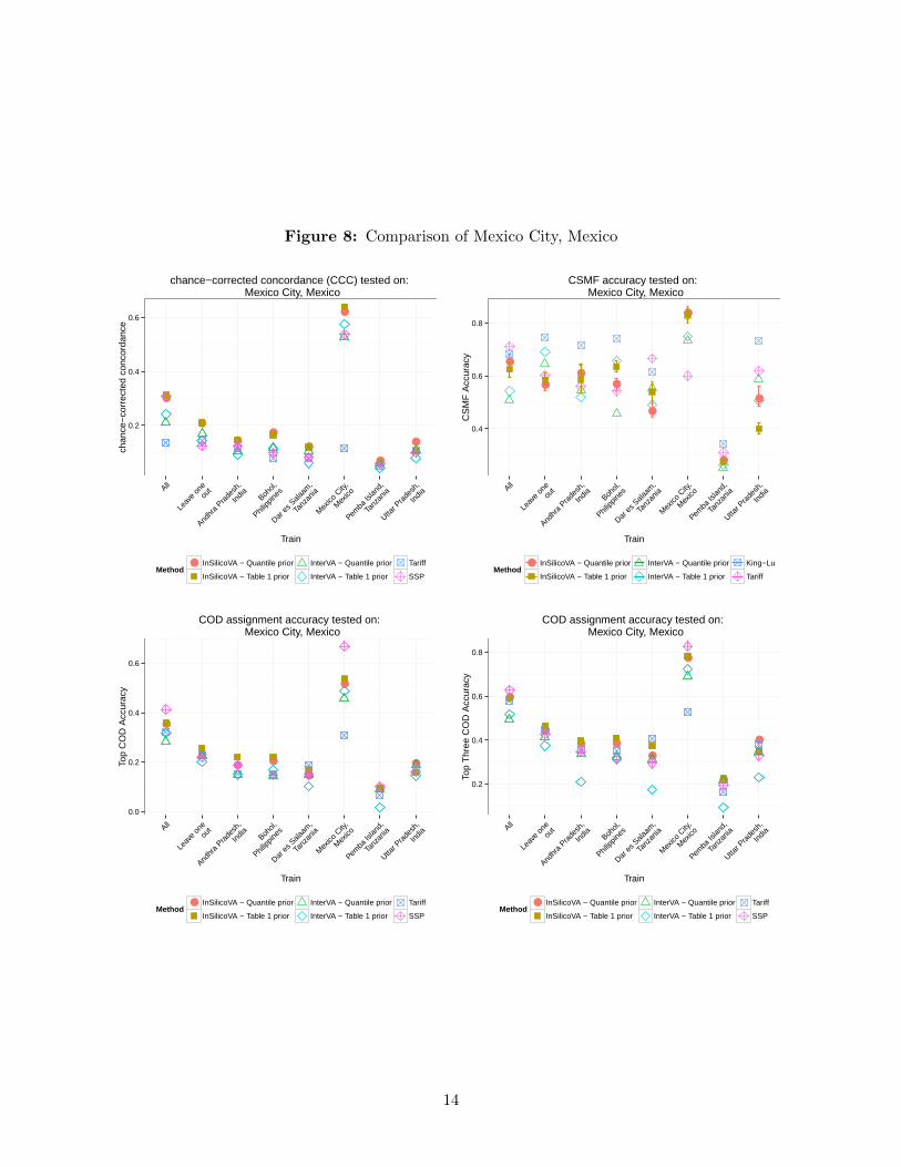
Figure 8: Comparison of Mexico City, Mexico

●

●

●●

●

●

●

●

0.2

0.4

0.6

All

Leav

e on

eou

t

Andhr

a Pra

desh

,

India Boh

ol,

Philipp

ines

Dar e

s Sala

am,

Tanz

ania

Mex

ico C

ity,

Mex

ico

Pemba

Islan

d,

Tanz

ania

Uttar P

rade

sh,

India

Train

chan

ce−

corr

ecte

d co

ncor

danc

e





Tariff

SSP

chance−corrected concordance (CCC) tested on: Mexico City, Mexico

●

●

●●

●

●

●

●

0.4

0.6

0.8

All

Leav

e on

eou

t

Andhr

a Pra

desh

,

India Boh

ol,

Philipp

ines

Dar e

s Sala

am,

Tanz

ania

Mex

ico C

ity,

Mex

ico

Pemba

Islan

d,

Tanz

ania

Uttar P

rade

sh,

India

Train

CS

MF

Acc

urac

y





King−Lu

Tariff

CSMF accuracy tested on: Mexico City, Mexico

●

●● ●

●

●

●

●

0.0

0.2

0.4

0.6

All

Leav

e on

eou

t

Andhr

a Pra

desh

,

India Boh

ol,

Philipp

ines

Dar e

s Sala

am,

Tanz

ania

Mex

ico C

ity,

Mex

ico

Pemba

Islan

d,

Tanz

ania

Uttar P

rade

sh,

India

Train

Top

CO

D A

ccur

acy





Tariff

SSP

COD assignment accuracy tested on: Mexico City, Mexico

●

●

● ●

●

●

●

●

0.2

0.4

0.6

0.8

All

Leav

e on

eou

t

Andhr

a Pra

desh

,

India Boh

ol,

Philipp

ines

Dar e

s Sala

am,

Tanz

ania

Mex

ico C

ity,

Mex

ico

Pemba

Islan

d,

Tanz

ania

Uttar P

rade

sh,

India

Train

Top

Thr

ee C

OD

Acc

urac

y





Tariff

SSP

COD assignment accuracy tested on: Mexico City, Mexico

14

Figure 9: Comparison of Pemba Island, Tanzania

●

●●

●● ●

●

●

0.0

0.2

0.4

0.6

0.8

All

Leav

e on

eou

t

Andhr

a Pra

desh

,

India Boh

ol,

Philipp

ines

Dar e

s Sala

am,

Tanz

ania

Mex

ico C

ity,

Mex

ico

Pemba

Islan

d,

Tanz

ania

Uttar P

rade

sh,

India

Train

chan

ce−

corr

ecte

d co

ncor

danc

e





Tariff

SSP

chance−corrected concordance (CCC) tested on: Pemba Island, Tanzania

●

●●

●

●

●

●

●

0.2

0.4

0.6

0.8

All

Leav

e on

eou

t

Andhr

a Pra

desh

,

India Boh

ol,

Philipp

ines

Dar e

s Sala

am,

Tanz

ania

Mex

ico C

ity,

Mex

ico

Pemba

Islan

d,

Tanz

ania

Uttar P

rade

sh,

India

Train

CS

MF

Acc

urac

y





King−Lu

Tariff

CSMF accuracy tested on: Pemba Island, Tanzania

●

● ●

●

●●

●

●

0.2

0.4

0.6

0.8

All

Leav

e on

eou

t

Andhr

a Pra

desh

,

India Boh

ol,

Philipp

ines

Dar e

s Sala

am,

Tanz

ania

Mex

ico C

ity,

Mex

ico

Pemba

Islan

d,

Tanz

ania

Uttar P

rade

sh,

India

Train

Top

CO

D A

ccur

acy





Tariff

SSP

COD assignment accuracy tested on: Pemba Island, Tanzania

●

●●

●

●

●

●

●

0.25

0.50

0.75

1.00

All

Leav

e on

eou

t

Andhr

a Pra

desh

,

India Boh

ol,

Philipp

ines

Dar e

s Sala

am,

Tanz

ania

Mex

ico C

ity,

Mex

ico

Pemba

Islan

d,

Tanz

ania

Uttar P

rade

sh,

India

Train

Top

Thr

ee C

OD

Acc

urac

y





Tariff

SSP

COD assignment accuracy tested on: Pemba Island, Tanzania

15

Figure 10: Comparison of Uttar Pradesh, India

●

● ●

● ●●

●

●

0.2

0.4

0.6

All

Leav

e on

eou

t

Andhr

a Pra

desh

,

India Boh

ol,

Philipp

ines

Dar e

s Sala

am,

Tanz

ania

Mex

ico C

ity,

Mex

ico

Pemba

Islan

d,

Tanz

ania

Uttar P

rade

sh,

India

Train

chan

ce−

corr

ecte

d co

ncor

danc

e





Tariff

SSP

chance−corrected concordance (CCC) tested on: Uttar Pradesh, India

●

●

●

●●

●

●

●

0.4

0.6

0.8

All

Leav

e on

eou

t

Andhr

a Pra

desh

,

India Boh

ol,

Philipp

ines

Dar e

s Sala

am,

Tanz

ania

Mex

ico C

ity,

Mex

ico

Pemba

Islan

d,

Tanz

ania

Uttar P

rade

sh,

India

Train

CS

MF

Acc

urac

y





King−Lu

Tariff

CSMF accuracy tested on: Uttar Pradesh, India

●

●●

● ●

●

●

●

0.2

0.4

0.6

All

Leav

e on

eou

t

Andhr

a Pra

desh

,

India Boh

ol,

Philipp

ines

Dar e

s Sala

am,

Tanz

ania

Mex

ico C

ity,

Mex

ico

Pemba

Islan

d,

Tanz

ania

Uttar P

rade

sh,

India

Train

Top

CO

D A

ccur

acy





Tariff

SSP

COD assignment accuracy tested on: Uttar Pradesh, India

●

●

●

●●

●

●

●

0.25

0.50

0.75

All

Leav

e on

eou

t

Andhr

a Pra

desh

,

India Boh

ol,

Philipp

ines

Dar e

s Sala

am,

Tanz

ania

Mex

ico C

ity,

Mex

ico

Pemba

Islan

d,

Tanz

ania

Uttar P

rade

sh,

India

Train

Top

Thr

ee C

OD

Acc

urac

y





Tariff

SSP

COD assignment accuracy tested on: Uttar Pradesh, India

16

3.1 Cause-specific performance

In this section we provide additional results for prediction performance for each cause. We comparethe average top cause accuracy (ACC1) for each of the four methods tested on 100 random splitof training and testing set with Dirichlet re-sampling. To reduce redundancy, for both InSilicoVAand InterVA we only report the version with conditional probabilities ranked by InterVA-4 cut-offvalues. The results are presented in Table 2. There are no methods dominating the accuracies forall causes. InSilicoVA has the highest accuracy for more than one third of the causes, achievingthe best performance among all methods. The confusion matrix for each methods is presented inFigure 11.

Figure 11: Confusion matrix for four methods.

Confusion matrix for InSilicoVA

Predicted Causes

True

Cau

ses

Esophageal CancerAsthma

Prostate CancerEpilepsy

Stomach CancerBite of Venomous Animal

PoisoningsColorectal Cancer

MalariaOther InjuriesLung Cancer

DrowningFires

SuicideCervical Cancer

Leukemia/LymphomasHomicide

COPDFalls

Breast CancerRoad Traffic

Diarrhea/DysenteryOther Infectious Diseases

TBCirrhosis

Acute Myocardial InfarctionDiabetes

Renal FailureOther Cardiovascular Diseases

MaternalAIDS

PneumoniaOther Non−communicable Diseases

Stroke

Str

oke

Oth

er N

on−

com

mun

icab

le D

isea

ses

Pne

umon

iaA

IDS

Mat

erna

lO

ther

Car

diov

ascu

lar

Dis

ease

sR

enal

Fai

lure

Dia

bete

sA

cute

Myo

card

ial I

nfar

ctio

nC

irrho

sis

TB

Oth

er In

fect

ious

Dis

ease

sD

iarr

hea/

Dys

ente

ryR

oad

Traf

ficB

reas

t Can

cer

Falls

CO

PD

Hom

icid

eLe

ukem

ia/L

ymph

omas

Cer

vica

l Can

cer

Sui

cide

Fire

sD

row

ning

Lung

Can

cer

Oth

er In

jurie

sM

alar

iaC

olor

ecta

l Can

cer

Poi

soni

ngs

Bite

of V

enom

ous

Ani

mal

Sto

mac

h C

ance

rE

pile

psy

Pro

stat

e C

ance

rA

sthm

aE

soph

agea

l Can

cer 0.0

0.2

0.4

0.6

0.8

1.0

Confusion matrix for InterVA

Predicted Causes

True

Cau

ses






DrowningFires



COPDFalls



TBCirrhosis



MaternalAIDS


Stroke

Str

oke

Oth

er N

on−

com

mun

icab

le D

isea

ses

Pne

umon

iaA

IDS

Mat

erna

lO

ther

Car

diov

ascu

lar

Dis

ease

sR

enal

Fai

lure

Dia

bete

sA

cute

Myo

card

ial I

nfar

ctio

nC

irrho

sis

TB

Oth

er In

fect

ious

Dis

ease

sD

iarr

hea/

Dys

ente

ryR

oad

Traf

ficB

reas

t Can

cer

Falls

CO

PD

Hom

icid

eLe

ukem

ia/L

ymph

omas

Cer

vica

l Can

cer

Sui

cide

Fire

sD

row

ning

Lung

Can

cer

Oth

er In

jurie

sM

alar

iaC

olor

ecta

l Can

cer

Poi

soni

ngs

Bite

of V

enom

ous

Ani

mal

Sto

mac

h C

ance

rE

pile

psy

Pro

stat

e C

ance

rA

sthm

aE

soph

agea

l Can

cer 0.0

0.2

0.4

0.6

0.8

1.0

Confusion matrix for Tariff

Predicted Causes

True

Cau

ses






DrowningFires



COPDFalls



TBCirrhosis



MaternalAIDS


Stroke

Str

oke

Oth

er N

on−

com

mun

icab

le D

isea

ses

Pne

umon

iaA

IDS

Mat

erna

lO

ther

Car

diov

ascu

lar

Dis

ease

sR

enal

Fai

lure

Dia

bete

sA

cute

Myo

card

ial I

nfar

ctio

nC

irrho

sis

TB

Oth

er In

fect

ious

Dis

ease

sD

iarr

hea/

Dys

ente

ryR

oad

Traf

ficB

reas

t Can

cer

Falls

CO

PD

Hom

icid

eLe

ukem

ia/L

ymph

omas

Cer

vica

l Can

cer

Sui

cide

Fire

sD

row

ning

Lung

Can

cer

Oth

er In

jurie

sM

alar

iaC

olor

ecta

l Can

cer

Poi

soni

ngs

Bite

of V

enom

ous

Ani

mal

Sto

mac

h C

ance

rE

pile

psy

Pro

stat

e C

ance

rA

sthm

aE

soph

agea

l Can

cer 0.0

0.2

0.4

0.6

0.8

1.0

Confusion matrix for SSP

Predicted Causes

True

Cau

ses






DrowningFires



COPDFalls



TBCirrhosis



MaternalAIDS


Stroke

Str

oke

Oth

er N

on−

com

mun

icab

le D

isea

ses

Pne

umon

iaA

IDS

Mat

erna

lO

ther

Car

diov

ascu

lar

Dis

ease

sR

enal

Fai

lure

Dia

bete

sA

cute

Myo

card

ial I

nfar

ctio

nC

irrho

sis

TB

Oth

er In

fect

ious

Dis

ease

sD

iarr

hea/

Dys

ente

ryR

oad

Traf

ficB

reas

t Can

cer

Falls

CO

PD

Hom

icid

eLe

ukem

ia/L

ymph

omas

Cer

vica

l Can

cer

Sui

cide

Fire

sD

row

ning

Lung

Can

cer

Oth

er In

jurie

sM

alar

iaC

olor

ecta

l Can

cer

Poi

soni

ngs

Bite

of V

enom

ous

Ani

mal

Sto

mac

h C

ance

rE

pile

psy

Pro

stat

e C

ance

rA

sthm

aE

soph

agea

l Can

cer 0.0

0.2

0.4

0.6

0.8

1.0

17

Table 2: Cause-specific accuracy of top predicted cause by four methods. Method with highestaccuracy for each cause is highlighted. The causes are arranged in decreasing order ofCSMFs.

CSMF InSilicoVA InterVA Tariff SSP

Stroke 0.0803 0.5085 0.4358 0.3796 0.3344Other Non-communicable Diseases 0.0764 0.0073 0.0032 0.0110 0.0776

Pneumonia 0.0689 0.0891 0.0433 0.0184 0.0887AIDS 0.0640 0.1665 0.4668 0.4405 0.6005

Maternal 0.0597 0.8360 0.5542 0.5371 0.0796Other Cardiovascular Diseases 0.0531 0.1052 0.0278 0.0552 0.1338

Renal Failure 0.0531 0.0862 0.0950 0.0446 0.0518Diabetes 0.0528 0.3537 0.3689 0.3084 0.5041

Acute Myocardial Infarction 0.0510 0.4350 0.2261 0.3422 0.3355Cirrhosis 0.0399 0.5314 0.7180 0.3349 0.0502

TB 0.0352 0.5270 0.3527 0.4784 0.4880Other Infectious Diseases 0.0335 0.0706 0.0669 0.1118 0.0654

Diarrhea/Dysentery 0.0291 0.3138 0.0647 0.2893 0.0220Road Traffic 0.0258 0.4482 0.2763 0.7173 0.0093

Breast Cancer 0.0249 0.7164 0.7596 0.6689 0.2316Falls 0.0221 0.1941 0.2308 0.4349 0.0042

COPD 0.0218 0.3840 0.4504 0.5560 0.3246Homicide 0.0213 0.5124 0.4824 0.7054 0.1321

Leukemia/Lymphomas 0.0199 0.2506 0.2761 0.2081 0.1040Cervical Cancer 0.0198 0.6701 0.4185 0.4833 0.3102

Suicide 0.0158 0.3093 0.1758 0.2684 0.1524Fires 0.0156 0.2745 0.2506 0.7114 0.0331

Drowning 0.0135 0.8116 0.6085 0.6034 0.3430Lung Cancer 0.0135 0.3700 0.6201 0.3666 0.0926

Other Injuries 0.0131 0.5346 0.3755 0.5853 0.0804Malaria 0.0128 0.2543 0.0295 0.3148 0.1842

Colorectal Cancer 0.0126 0.0795 0.1218 0.2743 0.0201Poisonings 0.0110 0.2991 0.3119 0.2903 0.0127

Bite of Venomous Animal 0.0084 0.8003 0.5008 0.9042 0.1294Stomach Cancer 0.0079 0.2458 0.2953 0.1537 0.0574

Epilepsy 0.0061 0.5628 0.5225 0.4209 0.1842Prostate Cancer 0.0061 0.4105 0.1728 0.0875 0.0455

Asthma 0.0060 0.3865 0.1219 0.1925 0.2661Esophageal Cancer 0.0051 0.5194 0.2536 0.1797 0.2161

18

4 Prior sensitivity analysis

We need to choose is the strength of the truncated beta distribution for the conditional probabilitytables. For the normal prior on transformed CSMF parameter θk, we put a diffuse uniform priorson hyper-parameter µ and σ2 so that no prior knowledge of the whole CSMF distribution is neededwhen fitting the model, which is usually the case in practice. In this section, we demonstrate theinfluence of (1) different prior means and (2) different prior variances of PL(s|c). We show boththe changes in posterior distribution of PL(s|c) and in the estimated CSMF. Finally we show thenumber of levels does not affect the results for the algorithm very much.

Prior means of PL(s|c) In the model, the truncated beta prior for PL(s|c) is specified such that

PL(s|c) ∼ Beta(αs|c,M − αs|c) and PL(s|c) ∈ (PL(s|c)−1, PL(s|c)+1).

We first evaluated the different choices of αs|c on the fitted results. We ran the model on thewhole PHMRC dataset, using the conditional probability matrix extracted from the same data andranked by quantile (described in Section 2.4.4). Instead of using the median value in each level asthe prior mean

αs|cM , we instead assign an ordered random vector between 0 and 1 for each level of

αs|cM . In our experiment, we sampled from a truncated Exponential(1) distribution 10 times with

fixed M and performed the analysis. It could be seen from Figure 12 that even the prior mean israndomly assigned, InSilicoVA successfully found the posterior mean close to truth. It should benoticed that since the real PS|C matrix is not in ranked form, the red reference line in Figure 12are only the median of the binned probabilities in each level, thus it is acceptable as long as theposteriors are close to them. Firgure 13 shows CSMF accuracy for each of the 10 simulations. Itcould be seen most of the bars overlap, and all ranges mostly between 0.70 to 0.74, indicating similarperformances. Figure 14 shows most of the CSMF distributions does not change dramatically giventhe very different prior mean specifications either.

Prior variance of PL(s|c) The strength of prior is specified through the constant M . When the

prior meanαs|cM is fixed, larger M imposes stronger belief on the prior mean. Since the posterior of

PL(s|c)|S, ~y depends on the sample size N in the data (see main text for detail), we compared the

influence of MN on both the CSMF (see Figure 15) and the estimated PL(s|c) vector (see Figure 16).

The fitted CSMF is relatively more sensitive to the ratio of MN , which is as expected since it affects

the posterior distribution of P (S|C) matrix. As could be seen from Figure 16, increasing the ratiowill lead to posterior samples closer to prior mean.

Number of levels in PL(s|c) The number of levels in PL(s|c) is set at 15 in all other sections ofthe paper and supplementary material. We show here changing the number of levels does not affectthe results by much. We again use the whole PHMRC dataset to generate a conditional probabilitymatrix and use it to fit the model on the dataset itself. When generating the ranked conditionalprobability matrix, we now order every value in the empirical conditional probability matrix, andbin them in into K bins so that each bin contains the same number of cells. We then assign eachbin a letter level and use the median value in it as the prior mean. The CSMF accuracy is presentedin Figure 17. It could be seen that the CSMF accuracy remains at a roughly the same level whenthe number of levels is greater than 15.

19

Figure 12: Prior and posterior of PL(s|c) in 10 simulations. The blue circles are the prior meanand the black dots with error bars are the posterior distribution. The red lines are themedian value within each level in real data.

2 4 6 8 10

0.6

0.8

1.0

level I

Simulation

Pro

babi

lity

●●

●●

●

●

●●

●●

●●

●●

●

●

●

●

●

●

2 4 6 8 10

0.6

0.8

level A+

Simulation

Pro

babi

lity ●● ●

●

●

●

●

●

●● ●

●

●

●

●

●

●

●●

●

2 4 6 8 10

0.5

0.7

0.9

level A

Simulation

Pro

babi

lity

●

●

●●

●

●

●

●

●

●

●

●

●

●

●

●

●

●

●

●

2 4 6 8 10

0.4

0.6

0.8

level A−

Simulation

Pro

babi

lity

●●

●●

●

●

●

●

●

●

●

●

●●

●●

●

●

●

●

2 4 6 8 10

0.4

0.6

level B+

Simulation

Pro

babi

lity

●● ●● ●

●

●

●

●●

●

●

●

●

●

●

●

●

●

●

2 4 6 8 10

0.3

0.5

level B

Simulation

Pro

babi

lity

●

●

●● ●●

●

●

●● ●

●

●

●

●

●

●

●

●

●

2 4 6 8 10

0.3

0.5

level B−

Simulation

Pro

babi

lity

●

●

●

●

●

●

●

●

●

●

●

●

●●

●

●

●

●

●●

2 4 6 8 10

0.20

0.35

0.50

level C+

Simulation

Pro

babi

lity

●

●

●

●

●

●

●● ●

●

●

●

●

●

●

●

●

●

●●

2 4 6 8 10

0.15

0.30

0.45

level C

Simulation

Pro

babi

lity

●

●

●

●

●

●

●●

●

●

●

●

●● ●

●

●●

●

●

2 4 6 8 10

0.10

0.25

0.40

level C−

Simulation

Pro

babi

lity

●

●

●

●

●

●

●

●

●

●

●

●

●

●

●

●

●

●

●

●

2 4 6 8 10

0.10

0.20

level D+

Simulation

Pro

babi

lity

●

●

●

●

●

●

●

●

●

●

●

●

●

●

●

●

●

●

●

●

2 4 6 8 10

0.05

0.15

level D

Simulation

Pro

babi

lity

●

●

●

●

●

●

●

●

●

●

●

●

●

●

●

●

●

●

●

●

2 4 6 8 10

0.05

0.15

level D−

Simulation

Pro

babi

lity

●

●

●

●

●

●

●

●

●

●

●

●

●

●

●

●

●

●

●

●

2 4 6 8 100.

000.

040.

080.

12

level E

Simulation

Pro

babi

lity

●

●

●

●

●

●

●

●

●

●

●

●

●

●

●

●

●

●●

●

2 4 6 8 10

0.00

0.04

0.08

level N

Simulation

Pro

babi

lity

●

●

●

●

●

●

●●

●

●

●

●

●

●

●

●

●●

●

●

Figure 13: CSMF accuracy distributions in 10 simulations, ordered by the mean accuracy in eachsimulations. The red dotted lines are the 95% confidence interval for the accuracymetric across all 10 simulations

●●●●●●●

●●●●

1 2 3 4 5 6 7 8 9 10

0.68

0.69

0.70

0.71

0.72

0.73

0.74

0.75

CSMF Accuracy for 10 simulations

simulations

CS

MF

Acc

urac

y

20

Figure 14: Top 12 CSMFs in 10 simulations. The blue dotted lines are the mean value across all10 simulations

●●●●●●

●●●●●●●●●●●●●●●●●●●●●●●●●●●●●●●●●●

●●●●●●●●●●●●●●●●●●●●●●●●●●●●●●●

●

●●●●●●●●●●●●●●●●●●●●●●●●●●

●●●●●●●●

●●

●●●●●●●●●●●●●●●●●

●●●●●●●●●●●●●●

1 2 3 4 5 6 7 8 9 10

0.07

00.

080

0.09

0

Maternal

simulation

CS

MF

●●●●●●●●●●●●●●●●●●●●●●

●●●●●●●●●●●●●●●●●●●●●●●●●●●●●●●●●●●●●●●

●

●●●●●●●●●●●●●●●●●●●●

●●●●●●●●●●●●●●

●●●●●●●●●

●●●

●●●●●●●●●●●

●●●●●●●●●●●●●●●●●●●●●●

●●●●●●●●

1 2 3 4 5 6 7 8 9 10

0.06

50.

080

Stroke

simulation

CS

MF

●●●●●●●●●●●●●●●●●●●●●●●●●●

●●●●●●●●●●●●●●●●●●●●●●

●●●●●●●●●●●●●●●●●●●●●●●

●●●●●●●

●●●●●●●

●●●●●●●●●

●●●●●●●●●●●●●●●●●●●●●●●●●●●●●●●●●

●●●●●●●●●●●●●●●●●●●●●●

1 2 3 4 5 6 7 8 9 10

0.06

00.

070

TB

simulation

CS

MF

●● ●●●●●●●●●●●●●●●●●●●●●●●●●●●●●●

●●●●●●●●●●●●●●●●●●●●●●●●●●

●●●●●

●●●●●

●●●●●●●●

1 2 3 4 5 6 7 8 9 10

0.05

00.

060

0.07

0

Cirrhosis

simulation

CS

MF

●●●●●

●●●●●●●●●●●●●●●●●●●●●●

●●●●

●●●●●●●

●●●●●●●●●●●●●●●●●●●●●●●●●●●●●●●●

●●●●●

●●●●

●●●●

●●●●●●●●●●

●●●●●●●●●●●●●●●●●●●●●●●●●●●●●●●●●●

●●●●●●●●● ●

1 2 3 4 5 6 7 8 9 10

0.04

50.

055

0.06

5

Acute Myocardial Infarction

simulation

CS

MF

●●●●●●●●●●●●●●●●●●●●●●●●●●●●●●●●●

●●●●●●●●●●●●●●●●●●●●●●●●●●●●●●

●●●●●●●●●●●●●●●●●●●●●●●●●●

●●●●●

●●●●●

1 2 3 4 5 6 7 8 9 10

0.04

50.

055

Malaria

simulationC

SM

F

●●●●●●●●●●●●●●●●●●●●●● ●●●●●●●●●

●●●●●●●●●●●●●●●●●●●●●●●●●●●●●●●●●●●●●●●●●●●●

●●●●●●●

●●●●●●●

●●●●●●●●●

●●●●●●●●●●●●●●●

●●●●●●●●●●●●●●●●●

●●●●●●●●●●●●●●●●●●●●●●●●●●

●●●●●●●●●●

●●●●●●●● ●●●●●

●●●●●●●●●●●●●●

1 2 3 4 5 6 7 8 9 10

0.03

50.

045

Diabetes

simulation

CS

MF

●●●●●●●●●●●●●●

●●●●●●●●●●●●●●●●●●●●●●●

●●●●

●●●●●●●●●

●●

●●●●●●●●●●●●●

●●●●●●●●●●●●●●●●●●●●●●●●●●

●●●●●

●●●●●

●●●●●●●●

1 2 3 4 5 6 7 8 9 10

0.03

00.

040

Road Traffic

simulation

CS

MF

●●●●●●●●●●●●●

●●●●●●●●●●●●●●●●●●●●●●

●●●●●●●●●●●●●●●●●●●●

●●●●●●●●●●●

●●●●●●●●●●●●●

●●●●●

●●●●

●●●●●●●●●●●●●●●●●●●●●●●●●●●●●●●

●●●●●●●●●

●

●●●●●●●●●●●●●●●●●●●●●●●●●●●●●●●●

●●●●●●●●●●●●●●●●●●●●●●●●●●

●

●●●●●

●●●●●●●●●●●●●●●●

●●●●●●●●●

●●●●●

●●●●●●●●●

●●●●●●●●●●●●●●●●●●●●●●●●●●●●●●●●●●

1 2 3 4 5 6 7 8 9 10

0.03

00.

040

Pneumonia

simulation

CS

MF

●●●●●●●●●●●●●●●●●●●●●●

●●●●●●●●●●●●●●●●●●●●●●●●●●●●

●●●●●●●●●●●●●●●●●●●●●●●●●●●●●●●

●●●●●●●●●●●

●●●●●●●●●●●●●

●●●●●●●●●●●●●●●●●●●●●●●●●●●●●●●●●

●●●

●●●●●●●●●●●

●●●●●●●●●●●●●●●●●●●●●●

●●●●●●●●●●●●●●●●●●●●●

●

●●●●●

●●●●●●●

1 2 3 4 5 6 7 8 9 10

0.03

00.

040

Cervical Cancer

simulation

CS

MF

●●●●●●●

●●●●●

●●●●●●●●●●●●●●●●●●●●●●●●●●●●●●●●●●●

●

●●●●●●●●●●●●●●●●●●●●●●●●●●

●●●●●

1 2 3 4 5 6 7 8 9 10

0.02

50.

035

0.04

5

Diarrhea/Dysentery

simulation

CS

MF

●●●●●●●●●●●

●●●●●

●●●●●

●●●●●●●●●

●●●●●

●●●●●●●●●

1 2 3 4 5 6 7 8 9 10

0.02

60.

032

0.03

8

Breast Cancer

simulation

CS

MF

21

Figure 15: top 12 CSMF distributions in simulations using different M . . The blue dotted linesare the mean value across all 6 simulations

●●

●●●●●●●●●

●●●●●●●●●●●●●●●●●●●●●●●●●●

●●●●●●●●●●●●●●●●●●●●●●●●●●●●●●

●●●●●●●●●●●●●●●●●●●

●●●●●●●●●●●●●●●●●●●●●●●●●●●●●●●●●●●●●

0.07

50.

085

Maternal

M/N

CS

MF

0.1 0.5 1 5 10 50

●●●●●●●●●●●●●●●●●●●●●●●●●●●●●

●●●●●●●●●●●●●●●●●●●

●●●●●●●●●●●●●●●●●●●●●●●●●●●●●●●●●●●●●

0.07

00.

076

0.08

2

Stroke

M/N

CS

MF

0.1 0.5 1 5 10 50

●●●●●●●●●●●●●●●●●●●●●●●●●●●●●●●●●●●●●●●●●●●●●●●●●●●●●●●●●●●●●

●●

●●●●●●●●●

●●●●●●●●●●●●●●●●●●●●●●●●●●

●●●●●●●●●●●●●●●●●●●●

●●●●●●●●●●●●●●●●●●●

●●●●●●●●●●●●●●●●●●●●●●●●●●●●●●●●●●●●●

0.06

00.

066

0.07

2

TB

M/N

CS

MF

0.1 0.5 1 5 10 50

●●●●●●●●●●●●●●●●●●●●●●●●●●●●●●●●●●●●●●●●●●●●●●●●●●●●●●●●●●

●●●●●●●●●●●●●●●●●●●

●●●●●●●●●●●●●●●●●●●●●●●●●●●●●●●●●●●●●

0.05

20.

058

0.06

4

Cirrhosis

M/N

CS

MF

0.1 0.5 1 5 10 50

●●●●●●●●●●●●●●●●●●●●●●●●●●●●●●●●●●●●●●●●●●●●●●●●●●●●●●●●●●●●●

●●

●●●●●●●●●

●●●●●●●●●●●●●●●●●●●●●●●●●●

●●●●●●●●●●●●●●●●●●●●

●●●●●●●●●●●●●●●●●●●●●●●●●●●●●●

●●●●●●●●●●●●●●●●●●●●●●●●●●●●●●●●●●●●●●●●●●●●●●

●●●●●●●●●●●●●●●●●●●●●●●●●●●●●●●●●●●●●●●●●●●●●●●●●●●●●●●●

0.05

40.

060

Acute Myocardial Infarction

M/N

CS

MF

0.1 0.5 1 5 10 50

●●●●●●●●●●●●●●●●●●●●●●●●●●●●●●●●●●●●●●●●●●●●●●●●●●●●●●●●●●

●●●●●●●●●●●●●●●●●●●●●●●●●●●●●●●●●●●

●●●●●●●●●●●●●●●●●●●

●●●●●●●●●●●●●●●●●●●●●●●●●●●●●●●●●●●●●

0.04

50.

055

Malaria

M/NC

SM

F0.1 0.5 1 5 10 50

●●●●●●●●●●●●●●●●●●●●●●●●●●●●●●●●●●●●●●●●●●●●●●●●●●●●●●●●●●

●●

●●●●●●●●●

●●●●●●●●●●●●●●●●●●●●●●●●●●

●●●●●●●●●●●●●●●●●●●●

●●●●●●●●●●●●●●●●●●●

●●●●●●●●●●●●●●●●●●●●●●●●●●●●●●●●●●●●●

0.03

80.

044

0.05

0

Diabetes

M/N

CS

MF

0.1 0.5 1 5 10 50

●●●●●●●●●●●●●●●●●●●●●●●●●●●●●●●●●●●●●●●●●●●●●●●●●●●●●●●●●●●●●

●●●●●●●●●●●

●●●●●●●●●●●●●●●●●●●●

●●●●●●●●●●●●●●●●●●●●●●●●●●●●●●●●●●●●●●●●●●●●●●

●●●●●●●●●●●●●●●●●●● ●●●●●●●●●●●●●●●●●●●●●●●●●●●●●●●●●●●●●

0.03

40.

040

0.04

6

Pneumonia

M/N

CS

MF

0.1 0.5 1 5 10 50

●●●●●●●●●●●●●●●●●●●●●●●●●●●●●●●●●●●●●●●●●●●●●●●●●●●●●●●●●●●●●

●●●●●●●●●●●●●●●●●●●

●●●●●●●●●●●●●●●●●●●●●●●●●●●●●●●●●●●●●

0.03

00.

040

Other Injuries

M/N

CS

MF

0.1 0.5 1 5 10 50

●●●●●●●●●●●●●●●●●●●●●●●●●●●●●●●●●●●●●●●●●●●●●●

●●●●●●●●●●●●●●●●●●●

●●●●●●●●●●●●●●●●●●●●●●●●●●●●●●●●●●●●●

0.03

00.

033

0.03

6

Road Traffic

M/N

CS

MF

0.1 0.5 1 5 10 50

●●●●●●●●●●●●●●●●●●● ●●●●●●●●●●●●●●●●●●●●●●●●●●●●●●●●●●●●●

0.02

50.

035

Diarrhea/Dysentery

M/N

CS

MF

0.1 0.5 1 5 10 50

●●●●●●●●●●●●●●●●●●●●●●●●●●●●

●●●●●●●●●●●●●●●●●●●

●●●●●●●●●●●●●●●●●●●●●●●●●●●●●●●●●●●●●0.02

90.

033

Breast Cancer

M/N

CS

MF

0.1 0.5 1 5 10 50

22

Figure 16: Prior and posterior of PL(s|c) with different M . The blue circles are the prior meanand the black dots with error bars are the posterior distribution. The red lines is theprior mean of each level, which is the median value within each level in real data.

0.95

0.97

0.99

level I

M/N

Pro

babi

lity

●

●

●

● ● ●

0.1 0.5 1 5 10 50

0.86

00.

870

level A+

M/N

Pro

babi

lity

●●

●● ● ●

0.1 0.5 1 5 10 50

0.72

0.74

0.76

level A

M/N

Pro

babi

lity

● ●●

●

●

●

0.1 0.5 1 5 10 500.

610.

63

level A−

M/NP

roba

bilit

y ●●

●

●

●

●

0.1 0.5 1 5 10 50

0.55

0.57

0.59

level B+

M/N

Pro

babi

lity ●

●

●

●

●

●

0.1 0.5 1 5 10 50

0.41

00.

425

0.44

0

level B

M/N

Pro

babi

lity

● ● ●

●

●

●

0.1 0.5 1 5 10 50

0.30

50.

320

level B−

M/N

Pro

babi

lity

●

●●

●●

●

0.1 0.5 1 5 10 50

0.28

00.

295

0.31

0

level C+

M/N

Pro

babi

lity ●

●●

●

●

●

0.1 0.5 1 5 10 50

0.16

00.

170

level C

M/N

Pro

babi

lity

● ● ●●

●

●

0.1 0.5 1 5 10 50

0.08

20.

086

level C−

M/N

Pro

babi

lity

●● ●

● ●●

0.1 0.5 1 5 10 50

0.07

60.

082

level D+

M/N

Pro

babi

lity

●● ●

● ● ●

0.1 0.5 1 5 10 50

0.03

30.

035

level D

M/N

Pro

babi

lity

● ● ● ● ●

●

0.1 0.5 1 5 10 50

0.00

90.

012

level D−

M/N

Pro

babi

lity

●●

●

● ●●

0.1 0.5 1 5 10 50

0.00

450.

0065

level E

M/N

Pro

babi

lity

● ● ●

●

●

●

0.1 0.5 1 5 10 50

0e+

004e

−04

level N

M/N

Pro

babi

lity ●

● ●

●

●

●

0.1 0.5 1 5 10 50

23

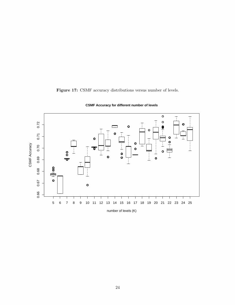
Figure 17: CSMF accuracy distributions versus number of levels.

●●●●●●●●●●●●●●●●●●●●

●●●●●

●●●●●●●●●●●●●

●●

●●●●●●●●●●●●●●●●●●●●

●●●●●●●●●●●●●●●●●●●●●●●●●●●●●●●●●

●●●●●●●●●●

●●●●●●

●●●●●●●●●●●●●●●●●●●●●●●●●

●●●●●●●●●●●●●●●●●●●●●●●●●●

●●●●●●●●●●●●●●●●●●●●●●●●●●●

●●●●●●●●●●●●●●●●●●●●●●●●●●●●●●●●●●●●●●●●●●●●●●●●●●●●●●●●●●●

●●●●●●●●●●●●●●●●●●●●●●●●●●●●●●●●●●●●●●●●●●●●●

●●●●●●●●●●●●●●●●●●●●●●●●●

●●●●●

●●●●●●●●●●●●●

●●●●●●●●●●●●●●●●●●

●●●●●●●●●●●●●●●●●●●●●●●●●●●●●●●

●●●

●●●●●●●●●●●●

●●●●●

●●

●●●●●●

●●

●●●●●●●●●●●●●

●●●●●●●

●●●●●●●●●●●●●

●●●●●●●●●●●●●●●●●●●●●●●●●●●●●●●●●●●●●●●●●●●●●●●●●●●●●

0.66

0.67

0.68

0.69

0.70

0.71

0.72

CSMF Accuracy for different number of levels

number of levels (K)

CS

MF

Acc

urac

y

5 6 7 8 9 10 11 12 13 14 15 16 17 18 19 20 21 22 23 24 25

24

5 Convergence analysis

5.1 Gelman-Rubin statistics

In this section we present the Gelman-Rubin statistics for both Agincourt and Karonga data. Wefocus on the convergence of CSMF that are greater than 0.01. The point estimates of the Gelman-Ruin statistics are mostly close to 1 for except for some causes with small fractions. In practicewe found the small CSMF values (less than 1%) do not converge well, though they only have veryminimum effect on the entire CSMF distribution. It should be improved with a larger data size.

Table 3: Gelman-Rubin statistics for Agincourt CSMF over 1%, arranged in descending order bythe mean.

Point est. Upper C.I.

HIV/AIDS related death 1.02 1.09Pulmonary tuberculosis 1.00 1.01

Severe malnutrition 1.06 1.19Diabetes mellitus 1.01 1.04

Acute resp infect incl pneumonia 1.11 1.35Other and unspecified cardiac dis 1.06 1.21Other and unspecified neoplasms 1.04 1.13Other and unspecified infect dis 1.08 1.23

Respiratory neoplasms 1.14 1.41Liver cirrhosis 1.07 1.22

Asthma 1.11 1.32Stroke 1.19 1.56

Table 4: Gelman-Rubin statistics for Karonga CSMF over 1%, arranged in descending order bythe mean.

Point est. Upper C.I.

Other and unspecified infect dis 1.01 1.05HIV/AIDS related death 1.00 1.01Other and unspecified neoplasms 1.04 1.12Pulmonary tuberculosis 1.03 1.10Digestive neoplasms 1.07 1.24Liver cirrhosis 1.01 1.03Other and unspecified cardiac dis 1.04 1.14Acute resp infect incl pneumonia 1.03 1.09Meningitis and encephalitis 1.14 1.46Acute abdomen 1.05 1.14

25

5.2 Trace plots

Figure 18: Trace plots for each CSMF posterior samples from three chains before thinning andincluding the burn-in period, arranged in descending order by the mean.

0 2000 4000 6000 8000 10000

0.05

0.15

0.25

0.35

HIV/AIDS related death

iterations

0 2000 4000 6000 8000 10000

0.05

0.15

0.25

Pulmonary tuberculosis

iterations

0 2000 4000 6000 8000 10000

0.00

0.04

0.08

0.12

Severe malnutrition

iterations

0 2000 4000 6000 8000 10000

0.02

0.06

0.10

Diabetes mellitus

iterations

0 2000 4000 6000 8000 10000

0.02

0.06

Acute resp infect incl pneumonia

iterations

0 2000 4000 6000 8000 10000

0.01

0.03

0.05

Other and unspecified cardiac dis

iterations

0 2000 4000 6000 8000 10000

0.01

0.03

0.05

Other and unspecified neoplasms

iterations

0 2000 4000 6000 8000 10000

0.01

0.03

Other and unspecified infect dis

iterations

0 2000 4000 6000 8000 10000

0.01

0.03

0.05

Respiratory neoplasms

iterations

0 2000 4000 6000 8000 10000

0.01

0.03

Liver cirrhosis

iterations

0 2000 4000 6000 8000 10000

0.00

00.

010

0.02

0

Asthma

iterations

0 2000 4000 6000 8000 10000

0.00

50.

010

0.01

5

Stroke

iterations

26

Figure 19: Trace plots for each CSMF posterior samples from three chains after thinning, arrangedin descending order by the mean.

0 50 100 150 200 250

0.25

50.

270

0.28

5


iterations

0 50 100 150 200 250

0.18

50.

195

0.20

5


iterations

0 50 100 150 200 250

0.09

00.

100

0.11

0

Severe malnutrition

iterations

0 50 100 150 200 250

0.06

00.

070

Diabetes mellitus

iterations

0 50 100 150 200 2500.

060

0.07

0


iterations

0 50 100 150 200 250

0.03

50.

040

0.04

50.

050


iterations

0 50 100 150 200 250

0.03

50.

040

0.04

5


iterations

0 50 100 150 200 250

0.02

50.

030

0.03

50.

040


iterations

0 50 100 150 200 250

0.01

40.

018

0.02

2


iterations

0 50 100 150 200 250

0.01

00.

014

Liver cirrhosis

iterations

0 50 100 150 200 250

0.01

00.

014

Asthma

iterations

0 50 100 150 200 250

0.00

80.

012

0.01

6

Stroke

iterations

Figure 20: Trace plots for each CSMF posterior samples from three chains before thinning andincluding the burn-in period, arranged in descending order by the mean.

0 2000 4000 6000 8000 10000

0.0

0.1

0.2

0.3

0.4


iterations

0 2000 4000 6000 8000 10000

0.05

0.15

0.25


iterations

0 2000 4000 6000 8000 10000

0.02

0.06

0.10

0.14


iterations

0 2000 4000 6000 8000 10000

0.02

0.06


iterations

0 2000 4000 6000 8000 10000

0.00

0.02

0.04

0.06

Digestive neoplasms

iterations

0 2000 4000 6000 8000 10000

0.02

0.06

Liver cirrhosis

iterations

0 2000 4000 6000 8000 10000

0.00

0.02

0.04


iterations

0 2000 4000 6000 8000 10000

0.01

0.03

0.05

0.07


iterations

0 2000 4000 6000 8000 10000

0.00

0.02

0.04

0.06

Meningitis and encephalitis

iterations

0 2000 4000 6000 8000 10000

0.00

00.

010

0.02

00.

030

Acute abdomen

iterations

27


0 50 100 150 200 250

0.32

0.36

0.40


iterations

0 50 100 150 200 250

0.18

0.20

0.22

0.24


iterations

0 50 100 150 200 250

0.06

0.10

0.14


iterations

0 50 100 150 200 250

0.04

0.06

0.08


iterations

0 50 100 150 200 250

0.03

0.05

0.07

Digestive neoplasms

iterations

0 50 100 150 200 250

0.03

0.04

0.05

0.06

Liver cirrhosis

iterations

0 50 100 150 200 250

0.01

50.

030

0.04

5


iterations

0 50 100 150 200 250

0.01

00.

020

0.03

0


iterations

0 50 100 150 200 250

0.01

00.

020


iterations

0 50 100 150 200 250

0.00

50.

015

0.02

5

Acute abdomen

iterations

28

5.3 Autocorrelation plots


0 5 10 15 20

0.0

0.2

0.4

0.6

0.8

1.0

Lag

AC

F


0 5 10 15 20

0.0

0.2

0.4

0.6

0.8

1.0

LagA

CF


0 5 10 15 20

0.0

0.2

0.4

0.6

0.8

1.0

Lag

AC

F


0 5 10 15 20

0.0

0.2

0.4

0.6

0.8

1.0

Lag

AC

F


0 5 10 15 20

−0.

20.

00.

20.

40.

60.

81.

0

Lag

AC

F


0 5 10 15 20

−0.

20.

00.

20.

40.

60.

81.

0

Lag

AC

F


0 5 10 15 20

0.0

0.2

0.4

0.6

0.8

1.0

Lag

AC

F

Severe malnutrition

0 5 10 15 20

0.0

0.2

0.4

0.6

0.8

1.0

Lag

AC

F

Severe malnutrition

0 5 10 15 20

0.0

0.2

0.4

0.6

0.8

1.0

Lag

AC

F

Severe malnutrition

0 5 10 15 20

0.0

0.2

0.4

0.6

0.8

1.0

Lag

AC

F

Diabetes mellitus

0 5 10 15 20

−0.

20.

00.

20.

40.

60.

81.

0

Lag

AC

F

Diabetes mellitus

0 5 10 15 20

0.0

0.2

0.4

0.6

0.8

1.0

Lag

AC

F

Diabetes mellitus

0 5 10 15 20

0.0

0.2

0.4

0.6

0.8

1.0

Lag

AC

F


0 5 10 15 20

0.0

0.2

0.4

0.6

0.8

1.0

Lag

AC

F


0 5 10 15 20

0.0

0.2

0.4

0.6

0.8

1.0

Lag

AC

F


0 5 10 15 20

0.0

0.2

0.4

0.6

0.8

1.0

Lag

AC

F


0 5 10 15 20

0.0

0.2

0.4

0.6

0.8

1.0

Lag

AC

F


0 5 10 15 20

0.0

0.2

0.4

0.6

0.8

1.0

Lag

AC

F


29

Figure 22(cont.): Trace plots for each CSMF posterior samples from three chains afterthinning, arranged in descending order by the mean.

0 5 10 15 20

0.0

0.2

0.4

0.6

0.8

1.0

Lag

AC

F


0 5 10 15 20

0.0

0.2

0.4

0.6

0.8

1.0

Lag

AC

F


0 5 10 15 20

0.0

0.2

0.4

0.6

0.8

1.0

Lag

AC

F


0 5 10 15 20

0.0

0.2

0.4

0.6

0.8

1.0

Lag

AC

F


0 5 10 15 20

0.0

0.2

0.4

0.6

0.8

1.0

Lag

AC

F


0 5 10 15 20

0.0

0.2

0.4

0.6

0.8

1.0

Lag

AC

F


0 5 10 15 20

−0.

20.

00.

20.

40.

60.

81.

0

Lag

AC

F


0 5 10 15 20

0.0

0.2

0.4

0.6

0.8

1.0

Lag

AC

F


0 5 10 15 20

0.0

0.2

0.4

0.6

0.8

1.0

Lag

AC

F


0 5 10 15 20

0.0

0.2

0.4

0.6

0.8

1.0

Lag

AC

F

Liver cirrhosis

0 5 10 15 20

−0.

20.

00.

20.

40.

60.

81.

0

Lag

AC

F

Liver cirrhosis

0 5 10 15 20

0.0

0.2

0.4

0.6

0.8

1.0

Lag

AC

F

Liver cirrhosis

0 5 10 15 20

0.0

0.2

0.4

0.6

0.8

1.0

Lag

AC

F

Asthma

0 5 10 15 20

0.0

0.2

0.4

0.6

0.8

1.0

Lag

AC

F

Asthma

0 5 10 15 20

0.0

0.2

0.4

0.6

0.8

1.0

Lag

AC

F

Asthma

0 5 10 15 20

0.0

0.2

0.4

0.6

0.8

1.0

Lag

AC

F

Stroke

0 5 10 15 20

0.0

0.2

0.4

0.6

0.8

1.0

Lag

AC

F

Stroke

0 5 10 15 20

0.0

0.2

0.4

0.6

0.8

1.0

Lag

AC

F

Stroke

30


0 5 10 15 20

0.0

0.2

0.4

0.6

0.8

1.0

Lag

AC

F


0 5 10 15 200.

00.

20.

40.

60.

81.

0

Lag

AC

F


0 5 10 15 20

−0.

20.

00.

20.

40.

60.

81.

0

Lag

AC

F


0 5 10 15 20

−0.

20.

00.

20.

40.

60.

81.

0

Lag

AC

F


0 5 10 15 20

0.0

0.2

0.4

0.6

0.8

1.0

Lag

AC

F


0 5 10 15 20

0.0

0.2

0.4

0.6

0.8

1.0

Lag

AC

F


0 5 10 15 20

0.0

0.2

0.4

0.6

0.8

1.0

Lag

AC

F


0 5 10 15 20

0.0

0.2

0.4

0.6

0.8

1.0

Lag

AC

F


0 5 10 15 20

0.0

0.2

0.4

0.6

0.8

1.0

Lag

AC

F


0 5 10 15 20

−0.

20.

00.

20.

40.

60.

81.

0

Lag

AC

F


0 5 10 15 20

0.0

0.2

0.4

0.6

0.8

1.0

Lag

AC

F


0 5 10 15 20

0.0

0.2

0.4

0.6

0.8

1.0

Lag

AC

F


0 5 10 15 20

0.0

0.2

0.4

0.6

0.8

1.0

Lag

AC

F

Digestive neoplasms

0 5 10 15 20

0.0

0.2

0.4

0.6

0.8

1.0

Lag

AC

F

Digestive neoplasms

0 5 10 15 20

0.0

0.2

0.4

0.6

0.8

1.0

Lag

AC

F

Digestive neoplasms

31

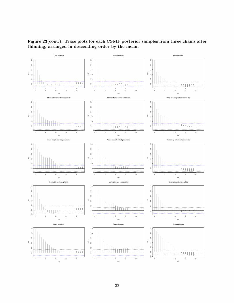
Figure 23(cont.): Trace plots for each CSMF posterior samples from three chains afterthinning, arranged in descending order by the mean.

0 5 10 15 20

0.0

0.2

0.4

0.6

0.8

1.0

Lag

AC

F

Liver cirrhosis

0 5 10 15 200.

00.

20.

40.

60.

81.

0

Lag

AC

F

Liver cirrhosis

0 5 10 15 20

0.0

0.2

0.4

0.6

0.8

1.0

Lag

AC

F

Liver cirrhosis

0 5 10 15 20

0.0

0.2

0.4

0.6

0.8

1.0

Lag

AC

F


0 5 10 15 20

0.0

0.2

0.4

0.6

0.8

1.0

Lag

AC

F


0 5 10 15 20

0.0

0.2

0.4

0.6

0.8

1.0

Lag

AC

F


0 5 10 15 20

0.0

0.2

0.4

0.6

0.8

1.0

Lag

AC

F


0 5 10 15 20

0.0

0.2

0.4

0.6

0.8

1.0

Lag

AC

F


0 5 10 15 20

0.0

0.2

0.4

0.6

0.8

1.0

Lag

AC

F


0 5 10 15 20

−0.

20.

00.

20.

40.

60.

81.

0

Lag

AC

F


0 5 10 15 20

0.0

0.2

0.4

0.6

0.8

1.0

Lag

AC

F


0 5 10 15 20

0.0

0.2

0.4

0.6

0.8

1.0

Lag

AC

F


0 5 10 15 20

0.0

0.2

0.4

0.6

0.8

1.0

Lag

AC

F

Acute abdomen

0 5 10 15 20

0.0

0.2

0.4

0.6

0.8

1.0

Lag

AC

F

Acute abdomen

0 5 10 15 20

−0.

20.

00.

20.

40.

60.

81.

0

Lag

AC

F

Acute abdomen

32

References

P. Byass, D. Chandramohan, S. Clark, L. D’Ambruoso, E. Fottrell, W. Graham, A. Herbst,A. Hodgson, S. Hounton, K. Kahn, A. Krishnan, J. Leitao, F. Odhiambo, O. Sankoh, andS. Tollman. Strengthening standardised interpretation of verbal autopsy data: the new interva-4tool. Global Health Action, 5(0), 2012.

N. Desai, L. Aleksandrowicz, P. Miasnikof, Y. Lu, J. Leitao, P. Byass, S. Tollman, P. Mee, D. Alam,S. K. Rathi, et al. Performance of four computer-coded verbal autopsy methods for cause of deathassignment compared with physician coding on 24,000 deaths in low-and middle-income countries.BMC medicine, 12(1):20, 2014.

S. L. James, A. D. Flaxman, C. J. Murray, and Consortium Population Health Metrics Research.Performance of the tariff method: validation of a simple additive algorithm for analysis of verbalautopsies. Popul Health Metr, 9(31), 2011.

G. King and Y. Lu. Verbal autopsy methods with multiple causes of death. Statistical Science,100(469), 2008.

D. Maher, S. Biraro, V. Hosegood, R. Isingo, T. Lutalo, P. Mushati, B. Ngwira, M. Nyirenda,J. Todd, and B. Zaba. Translating global health research aims into action: the example of thealpha network. Tropical Medicine & International Health, 15(3):321–328, 2010.

C. J. Murray, A. D. Lopez, D. M. Feehan, S. T. Peter, and G. Yang. Validation of the symptompattern method for analyzing verbal autopsy data. PLoS Medicine, 4(11):e327, 2007.

C. J. Murray, S. L. James, J. K. Birnbaum, M. K. Freeman, R. Lozano, A. D. Lopez, and Consor-tium Population Health Metrics Research. Simplified symptom pattern method for verbal autopsyanalysis: multisite validation study using clinical diagnostic gold standards. Popul Health Metr,9(30), 2011.

C. J. Murray, A. D. Lopez, R. Black, R. Ahuja, S. M. Ali, A. Baqui, L. Dandona, E. Dantzer, V. Das,U. Dhingra, et al. Population health metrics research consortium gold standard verbal autopsyvalidation study: design, implementation, and development of analysis datasets. Populationhealth metrics, 9(1):27, 2011.

C. J. Murray, R. Lozano, A. D. Flaxman, A. Vahdatpour, and A. D. Lopez. Robust metrics forassessing the performance of different verbal autopsy cause assignment methods in validationstudies. Popul Health Metr, 9(1):28, 2011.

C. J. Murray, R. Lozano, A. D. Flaxman, P. Serina, D. Phillips, A. Stewart, S. L. James, A. Vah-datpour, C. Atkinson, M. K. Freeman, et al. Using verbal autopsy to measure causes of death:the comparative performance of existing methods. BMC medicine, 12(1):5, 2014.

33

supplementary material: probabilistic cause-of-death ...tylermc/insilico_supplement_r1.pdf ·...

Documents