Supplementary Material for

Measuring Economic Activity in China with

Mobile Big Data

Lei Dong∗1,2,3, Sicong Chen2, Yunsheng Cheng2, Zhengwei Wu2, Chao Li2, andHaishan Wu†2

1Institute of Remote Sensing and Geographical Information Systems, PekingUniversity, Beijing, 100871, China

2Big Data Lab, Baidu Research, Baidu, Beijing, 100085, China3School of Architecture, Tsinghua University, Beijing, 100084, China

Data Access

All indices mentioned in the main text could be accessed via http://bdl.baidu.com/mobimetrics,or the Bloomberg Terminal.

Tags of POI

POI, or Points of Interest, refer to the geo-position points in maps. POI provided byBaidu Maps come from different sources. To assure the quality of POI, Baidu checkedthe validity of every POI and merged them into a standardized dataset. By comparingnames and spatial coordinates of POI, calculating similarities and hashing, Baidu builtits own POI dataset with a precision higher than 95%. All the POI were assigned withcorrect tags that described the attributes of locations. Each POI belongs to a standardizedtag, and there are 30 categories and about 240 subcategories in total. In our research, wechose categories related to consumer activities: such as Shopping, Financial Institutions,Hotels, Tourism, Restaurants, Auto Services, and Entertainments.

Spatial Distribution of AOI

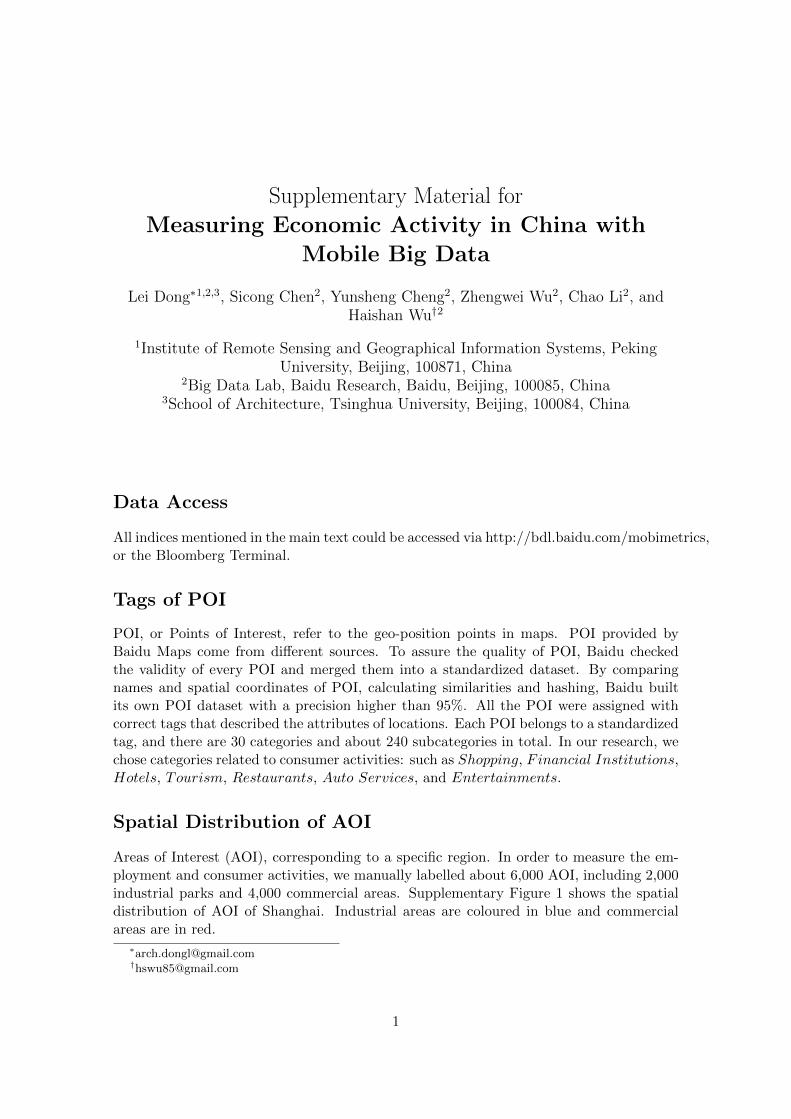
Areas of Interest (AOI), corresponding to a specific region. In order to measure the em-ployment and consumer activities, we manually labelled about 6,000 AOI, including 2,000industrial parks and 4,000 commercial areas. Supplementary Figure 1 shows the spatialdistribution of AOI of Shanghai. Industrial areas are coloured in blue and commercialareas are in red.

∗arch.dongl@gmail.com†hswu85@gmail.com

1

Supplementary Figure 1: (A) Illustration of the spatial distribution of labelled AOI. In-dustrial areas are coloured in blue and commercial areas are in red. Zoomed-in part: (B)and (C) are industrial parks and commercial areas, respectively. Maps were created byQGIS 2.12 (http://qgis.org/).

Parameters of DBSCAN

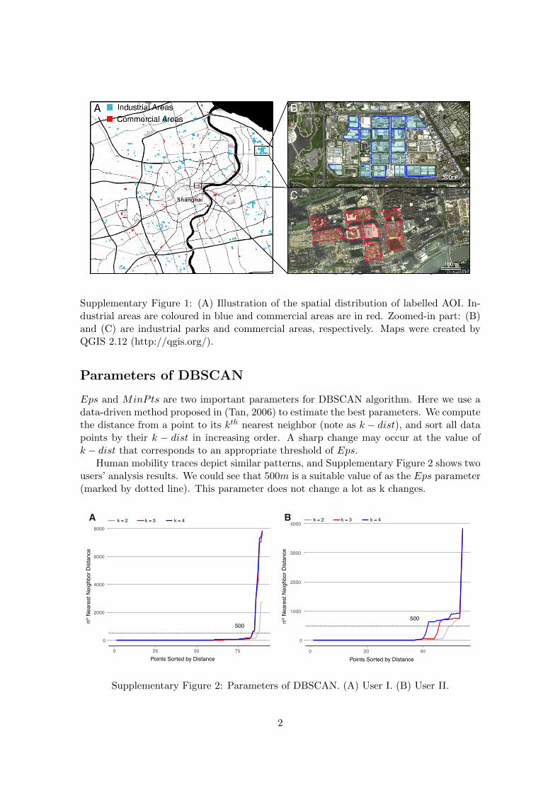
Eps and MinPts are two important parameters for DBSCAN algorithm. Here we use adata-driven method proposed in (Tan, 2006) to estimate the best parameters. We computethe distance from a point to its kth nearest neighbor (note as k − dist), and sort all datapoints by their k − dist in increasing order. A sharp change may occur at the value ofk − dist that corresponds to an appropriate threshold of Eps.

Human mobility traces depict similar patterns, and Supplementary Figure 2 shows twousers’ analysis results. We could see that 500m is a suitable value of as the Eps parameter(marked by dotted line). This parameter does not change a lot as k changes.

A B k = 2 k = 3 k = 4k = 2 k = 3 k = 4

500

0

1000

2000

3000

4000

0 20 40Points Sorted by Distance

nth N

eare

st N

eigh

bor D

ista

nce

nth N

eare

st N

eigh

bor D

ista

nce

500

0

2000

4000

6000

8000

0 25 50 75Points Sorted by Distance

Supplementary Figure 2: Parameters of DBSCAN. (A) User I. (B) User II.

2

Parameters of Consumer Detection

We use 10 minutes as the threshold to define a visit to a place in the main context. Tocheck whether the analysis change by varying this threshold, we set 5, 10, 15, 30 minutes asthe threshold respectively. Supplementary Figure 3 shows that the selection of thresholdhas little impact to the results.

A B5 min 10 min 30 min15 min 5 min 10 min 30 min15 min

0.4

0.6

0.8

1.0

0 10 20 30Time

Nor

mal

ized

Con

sum

ers

0.4

0.6

0.8

1.0

0 10 20 30Time

Nor

mal

ized

Con

sum

ers

Supplementary Figure 3: Time threshold and consumer detection. (A) AOI I. (B) AOI II.

Manufacturing Purchasing Management Index (PMI)

There are two main PMI data sources in China: One is published by National Bureau ofStatistics (NBS), the other one is called by Caixin PMI. In Supplementary Figure 4, weshow employment index derived from the NBS manufacturing PMI.

47.0

47.5

48.0

48.5

49.0

2014−01 2014−07 2015−01 2015−07 2016−01 2016−07Time

PMI

Supplementary Figure 4: National Bureau of Statistics Manufacturing Purchasing Man-agement Index (Employment Index) [Data source: http://data.stats.gov.cn].

3

The List of Selected Apple Stores

We selected POI of Apple Stores (China) based on the store list from Apple’s officialwebsite: https://www.apple.com/cn/retail/storelist/. Since Apple kept on expanding itsoffline stores in China, we only selected those opened before 2015y. The final list was asfollows:

• Beijing (Sanlitun, Dayuecheng, Wangfujing, Huamao)

• Shanghai (Guojin Center, Nanjing East Road, HongKong Plaza)

• Tianjin (Henglong Plaza)

• Chengdu (Wanxiangcheng)

• Wuxi (Henglong Plaza)

• Chongqing (Beichengtianjie)

• Shengzhen (Yitian Holiday Plaza)

The quarterly financial results were downloaded from: http://investor.apple.com/.

Map Query and Box Office

The baseline model for box office prediction is auto regression with 1 day and 7 day lags:

yt = β0 + β1yt−1 + β2yt−7 + et (1)

where yt, yt−1, and yt−7 are the revenues of box office at time t, t − 1, and t − 7,respectively. And the map query model is the baseline model plus map query variables:

yt = β1yt−1 + β2yt−7 + β3qt + β4qt−1 + β5qt−7 + et (2)

where q is the normalized (by page view) volume of map queries for cinemas.Results are shown in Supplementary Table 1. Map query improves the R2 of the

baseline model from 0.489 to 0.934.

Map Query Trends

As stated in the main text, the proposed map query trends are valuable for not onlyimproving forecasting accuracy, but also strengthening policy suggestions, which could befurther investigated through cross validation with more data sources.

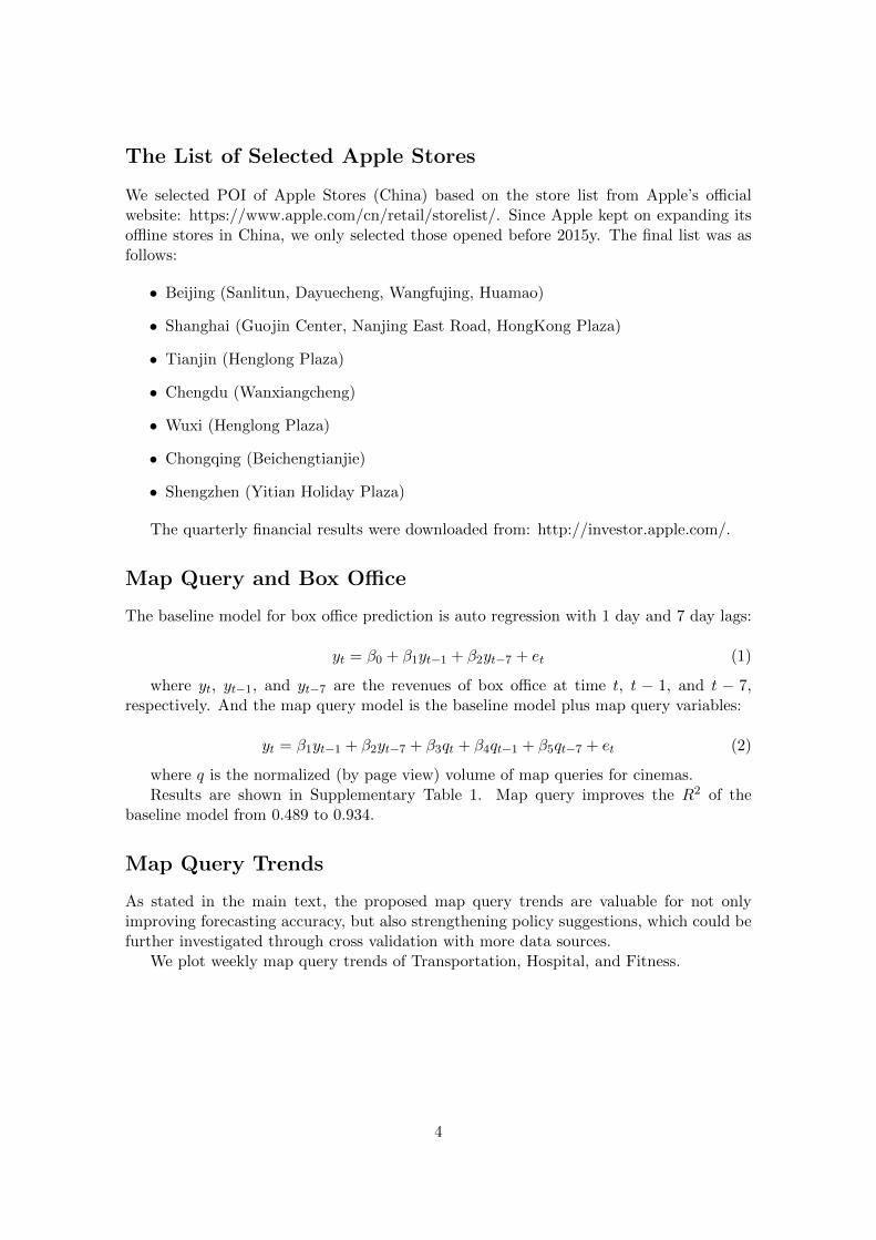
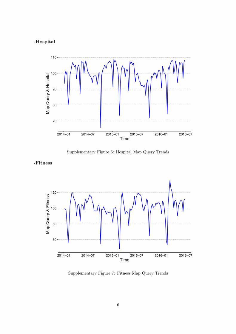
We plot weekly map query trends of Transportation, Hospital, and Fitness.

4

Variables Baseline Model + Map Query

yt−1 0.557*** 0.805***(0.041) (0.035)

yt−7 0.264*** 0.083(0.041) (0.034)

q 0.471***(0.010)

qt−1 -0.348***(0.019)

qt−7 -0.045***(0.017)

Observations 353 353R-squared 0.489 0.934

Note: OLS regressions are estimated with a con-stant that is not reported in this table. Standarderrors are shown in brackets. *** p < 0.001, **p < 0.01, * p < 0.05.

Supplementary Table 1: Regressions of foot trafficand map query

-Transportation

100

120

140

160

2014−01 2014−07 2015−01 2015−07 2016−01 2016−07Time

Map

Que

ry &

Tra

nspo

rtatio

n

Spring Festival (Chunyun)

National Holiday

Supplementary Figure 5: Transportation Map Query Trends.

5

-Hospital

70

80

90

100

110

2014−01 2014−07 2015−01 2015−07 2016−01 2016−07Time

Map

Que

ry &

Hos

pita

l

Supplementary Figure 6: Hospital Map Query Trends

-Fitness

60

80

100

120

2014−01 2014−07 2015−01 2015−07 2016−01 2016−07Time

Map

Que

ry &

Fitn

ess

Supplementary Figure 7: Fitness Map Query Trends

6

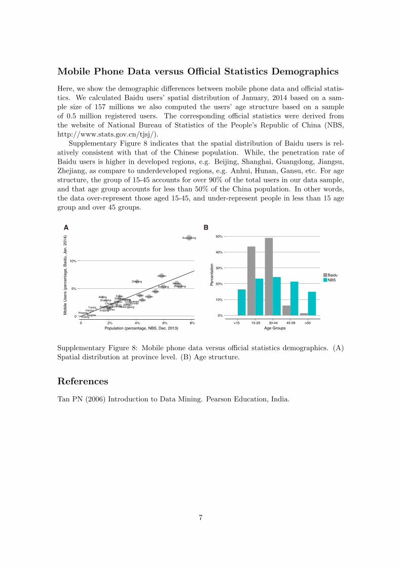
Mobile Phone Data versus Official Statistics Demographics

Here, we show the demographic differences between mobile phone data and official statis-tics. We calculated Baidu users’ spatial distribution of January, 2014 based on a sam-ple size of 157 millions we also computed the users’ age structure based on a sampleof 0.5 million registered users. The corresponding official statistics were derived fromthe website of National Bureau of Statistics of the People’s Republic of China (NBS,http://www.stats.gov.cn/tjsj/).

Supplementary Figure 8 indicates that the spatial distribution of Baidu users is rel-atively consistent with that of the Chinese population. While, the penetration rate ofBaidu users is higher in developed regions, e.g. Beijing, Shanghai, Guangdong, Jiangsu,Zhejiang, as compare to underdeveloped regions, e.g. Anhui, Hunan, Gansu, etc. For agestructure, the group of 15-45 accounts for over 90% of the total users in our data sample,and that age group accounts for less than 50% of the China population. In other words,the data over-represent those aged 15-45, and under-represent people in less than 15 agegroup and over 45 groups.

A B

0%

10%

20%

30%

40%

50%

<15 15-29 30-44 45-59 >50Age Groups

Perc

enta

tion

BaiduNBS

Beijing

Tianjin

Hebei

Shanxi

Neimenggu

Liaoning

Jilin Heilongjiang

Shanghai

Jiangsu

Zhejiang

AnhuiFujian

Jiangxi

ShandongHenan

Hubei Hunan

Guangdong

Guangxi

Hainan

Chongqing

Sichuang

GuizhouYunnan

Xizang

Shaanxi

Gansu

QinghaiNingxia

Xinjiang

0

5%

10%

0 2% 4% 6% 8%Population (percentage, NBS, Dec. 2013)

Mob

ile U

sers

(per

cent

age,

Bai

du, J

an. 2

014)

Supplementary Figure 8: Mobile phone data versus official statistics demographics. (A)Spatial distribution at province level. (B) Age structure.

References

Tan PN (2006) Introduction to Data Mining. Pearson Education, India.

7