supplementary information supplementary information … · recorders and manual measurements at...

SUPPLEMENTARY INFORMATIONDOI: 10.1038/NGEO1615

NATURE GEOSCIENCE | www.nature.com/naturegeoscience 1

Supplementary Information

for

Linking the historic 2011 Mississippi River flood to coastal wetland

sedimentation

Federico Falcini1,2,3, Nicole S. Khan1, Leonardo Macelloni4, Benjamin P. Horton1, Carol B.

Lutken4, Karen L. McKee5, Rosalia Santoleri2, Simone Colella2, Chunyan Li6, Gianluca

Volpe2, Marco D’Emidio4, Alessandro Salusti1,7, Douglas J. Jerolmack1*.

1 Department of Earth and Environmental Science, University of Pennsylvania, Philadelphia,

Pennsylvania 19104, USA.2Istituto di Scienze dell’ Atmosfera e del Clima, Consiglio Nazionale delle Ricerche, Rome

00133, Italy.3 St Anthony Falls Laboratory, and National Center for Earth-surface Dynamics, University

of Minnesota, Minneapolis, Minnesota 55414, USA.

4Mississippi Mineral Resources Institute, University of Mississippi, University, Mississippi

38677, USA.5 U. S. Geological Survey, National Wetlands Research Center, Lafayette, Louisiana 70506,

USA.6 Department of Oceanography and Coastal Sciences, School of the Coast and Environment,

Louisiana State University, Baton Rouge, Louisiana 70803, USA.7 Dipartimento Scienze Geologiche, Roma Tre, 00146 Rome, Italy.

*Corresponding Author. E-mail: [email protected]

Abstract.

We provide here supplementary materials such as methodologies, complementary data, and

theoretical and experimental analysis. Section 1 provides general information about the

historic 2011 Mississippi River (MR) flood and includes a review of various press releases

and hydrologic data from the U.S. Army Corps of Engineers and U.S. Geologic Survey.

Section 2 describes all the satellite, hydrographic and current meter data, providing

supporting analyses and sampling methodologies. We also present theoretical techniques for

the validation of the suspended sediment regime, the estimation of the suspended sediment,

and the Potential Vorticity theory which diagnoses the ability of the MR outflow to deliver

1

© 2012 Macmillan Publishers Limited. All rights reserved.

sediment offshore efficiently. Finally, Section 3 describes the marsh sediment sampling,

presenting supporting analyses and methodologies.

1. Background

The Historic 2011 Mississippi River (MR) Flood is among the largest floods of the past

century including, notably, those of 1927, 1973, and 1993 (Figure S1). In April 2011, the

MR watershed experienced the combination of two major storms and the springtime snow-

melt. By early May, the River began to swell to record levels (Figure 1d). According to the

United States Army Corps of Engineers, areas around Baton Rouge, LA were expected to be

inundated with 20-30 feet (6.1-9.1 m) of water1.

In order to avoid catastrophic floods, diversion of 3,500 m3/s of water from the Mis-

sissippi River to the Atchafalaya River Basin was planned (Figure 1d). The Morganza Spill-

way (Figures S1, S2), unused for nearly 40 years, was opened beginning on 14 May, 2011,

and operated at about 21% of its capacity1 (Figure S2), deliberately flooding 4,600 square

miles (12,000 km2) of rural Louisiana to protect Baton Rouge and New Orleans2. This diver-

sion also aimed to reduce floodwater stress on the Old River Control Structure (Figure S1),

a floodgate system that regulates the flow of water leaving the MR by diverting about 30%

of the MR flow into the Atchafalaya River (AR)3. In addition, the Bonnet Carre Spillway,

3 0 m i l e s n o r t h o f New Orleans, was opened to allow Mississippi River f l o od wa-

ters to drain into Lake Pontchartrain (Figure 1d, Figure S1)4..

In order to investigate the temporal evolution of water discharge and suspended sedi-

ment concentration (SSC) of the lower MR and AR, we examined USGS (National Water

Information System) surface water time-series data at Belle Chasse, LA and Morgan City,

LA, respectively (Figure 1d), over the range from April 1st to June 30th, 2011. SSC data for

the lower AR were collected at Simmesport, LA. These data were collected by automatic

2


recorders and manual measurements at field installations, and show that (Figure 1d): (i) SSC

for all sites peaked in about the 2nd week of May, i.e., ~10 days before the flood crest; (ii)

the two AR and Wax Lake samples had similar SSC to the MR at low discharge, but were

50% higher than MR at high discharge, a feature that may have been due to scouring of the

AR basin5.

We note that differences in the measured magnitude and spatial pattern of marsh sedi-

mentation that we report along the shoreline may have resulted from a variety of factors that

we do not examine here, e.g.: differences in relative elevation of marsh surfaces and duration

of flooding; the spatial distribution of natural or man-made barriers to water flows; differ-

ences in plant stem density that affects water flows and sediment trapping/resuspension; and

differential post-deposition reworking and erosion of sediment by waves or tides. It was not

possible to measure or account for these factors, which vary at a local scale beyond the scope

of our satellite-driven analysis. Accordingly, we examined spatial variations in coastal waters

– sea-surface temperature, suspended-sediment concentration, salinity, and velocity of ocean

currents – at kilometre to Delta scale, using satellite data calibrated to in-situ measurements

from a boat survey conducted around the Mississippi Birdsfoot Delta lobe. Although river

plume and coastal hydrodynamics are not the only important factors, we found a strong cor-

respondence between observed marsh sedimentation patterns and river plume sediment con-

centrations. In addition, we present a physical framework for nearshore dynamics that sup-

ports the hypothesis that sediment plume structure, along with the inundation pattern of

flooding, exerted a strong control on coastal deposition.

2. Measuring the MR sediment plume

Satellite data

3


We performed qualitative analyses of daily sea surface temperature (SST), and ocean true-

colour MODIS data from satellites to recognize river plume dispersion and sediment

migration paths in the nearshore zone for the MR and AR (Figure 1; Figure S3-SST-

ImageJ_MODIS daily), for period May 5 to June 5, 2011. Moreover, we processed and

analyzed MODIS Level-1A products containing the raw radiance counts from all bands, to

quantify the river plume patterns through time during the flood.

SST data are recorded by the Advanced Very High Resolution Radiometer

(AVHRR), a sensor operating onboard of the NOAA - POES series (Polar-Orbiting

Operational Environmental Satellites). The AVHRR sensor is a radiation-detection imager

that can be used for remotely determining the surface temperature of a body of water. This

scanning radiometer uses 6 detectors that collect different bands of radiation wavelengths

with a spatial resolution of 1.1 km [ref. 6]. Along-track wavelength data have to be processed

and interpolated in order to obtain high-resolution SST maps. For our work we used SST

maps provided by the Earth Scan Laboratory of the Louisiana State University7.

From SST data and from a detailed image statistical analysis of these SST, we

recognized that the two plumes from the MR and AR had distinctive characteristics: a diffuse

flow for the AR that remained close to the shoreline; and a filament-like jet for the MR that

penetrated far offshore with little apparent mixing (Figure S3), most notably that of the

Southwest Pass. The plumes can be recognized from the temperature contrast between the sea

water and the fresh, colder river water.

We also performed a similar comparative analysis by using ocean true-colour images

obtained from the Moderate Resolution Imaging Spectroradiometer (MODIS), a key

instrument aboard the Terra and Aqua satellites. Terra MODIS and Aqua MODIS view the

entire Earth's surface every 1 to 2 days and provide high radiometric sensitivity (12 bit) in 36

spectral bands ranging in wavelength from 0.4 µm to 14.4 µm. Two bands are imaged at a

4


nominal resolution of 250 m at nadir, with five bands at 500 m, and the remaining 29 bands at

1 km [ref. 8]. We employed MODIS images processed by the Institute of Marine Remote

Sensing of the University of South Florida9.

By using these near real-time MODIS true colour-images (Figure 1), it was possible

to track suspended sediment of the MR and AR plumes during the flood. This allowed us to

direct oceanographic surveys in real time, and thus to sample the plume velocity, suspended

sediment, and hydrologic features.

In order to make our plume analysis more quantitative, we then processed MODIS

Level-1A products by following a procedure for estimating suspended load from remote sens-

ing reflectance high resolution band 1 at 645nm [ref. 10]. MODIS images were downloaded

through the NASA Internet servers OceanColor Web. Data were processed using SeaDAS

MODIS commands, which generate level-1B products. The atmospheric correction was

performed by subtracting the minimum reflectance of band 2 at 859 nm to the band 1 at

645nm [ref. 10]. The algorithm consists of a linear equation that establishes a relationship

between field turbidity units (TU, see below) data and the corrected MODIS reflectance at

645 nm. The square correlation coefficient (R2=0.53; n=38) suggested a fairly good

relationship between these two parameters, indicating a correspondence between MODIS

reflectances and in situ TU. Based on this analysis the following algorithm was implemented:

SSC=1236 .74 ( MODIS_645)−34 .0692 . Using this field-calibrated SSC MODIS data, we

created two Hovmöller (space-time) plots of SSC, where the time evolution of both MR

Southwest Pass and AR plumes can be followed along two cross-plume transects perpendicu-

lar to the flow (Figure 1b,c). For the Southwest Pass we observed a plume width of about 20

km, as averaged through the flood period, while the AR plume width was ~40 km. Our ana-

lysis shows that the MR Southwest Pass sediment plume did not make contact with the

shoreline, remaining offshore and maintaining its filament-like character for the entire flood

5


period. The same analysis on the Atchafalaya plume shows a different pattern: sediment was

present along the shoreline in high concentration and decreased offshore, suggesting an

alongshore sediment flux that could have contributed to wetland sedimentation. Such a pat-

tern can be also observed more broadly from an SSC MODIS map for the survey day 1 June,

2011 (Figure 2c). Since we could not collect any suspended sediment data in the AR basin,

we warn the reader that the extrapolation of MR-calibrated MODIS SSC satellite images to

the AR may introduce errors; therefore, we use this analysis primarily to quantify the plume

patterns of both MR and AR systems, rather than to estimate an absolute value of SSC.

Finally, we present coastal current nowcast results from the South Atlantic Bight and

Gulf of Mexico Circulation Model (SABGOM) to compare plume dynamics to coastal dy-

namics. It is clear that a generally western coastal current pattern dominates for the flood,

with the largest magnitudes (almost 1 m/s) occurring in the vicinity of Southwest Pass (Fig-

ure S8). Nonetheless, the Southwest Pass sediment plume appears to penetrate deep offshore

with little influence, attesting to the lack of interaction of the MR plume with coastal cur-

rents. The AR sediment plume, on the other hand, appears to be strongly driven by the coastal

current – note the change in plume characteristics as the coastal current shifts from west to

south in Figure S8.

Boat Survey

A boat survey measured the currents and sediment concentrations of the MR plume

in-situ during the peak of the flood, from May 29 to June 1, 2011 (Figure S4). The diffuse

AR plume was not amenable to such a survey. The survey was aboard R/V Acadiana, a

Louisiana University Marine Consortium vessel outfitted for such work. Hydrographic

transects and station locations were based on the satellite analysis of the MR plume, and

communicated in quasi-real-time to the R/V. A hull-mounted Teledyne RD Instruments 600

kHz acoustic Doppler current profiler (ADCP) was used to measure velocity profiles

6


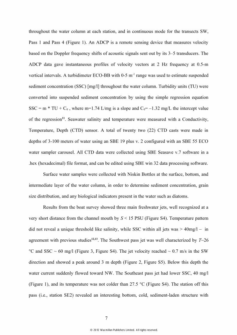
throughout the water column at each station, and in continuous mode for the transects SW,

Pass 1 and Pass 4 (Figure 1). An ADCP is a remote sensing device that measures velocity

based on the Doppler frequency shifts of acoustic signals sent out by its 3–5 transducers. The

ADCP data gave instantaneous profiles of velocity vectors at 2 Hz frequency at 0.5-m

vertical intervals. A turbidimeter ECO-BB with 0-5 m-1 range was used to estimate suspended

sediment concentration (SSC) [mg/l] throughout the water column. Turbidity units (TU) were

converted into suspended sediment concentration by using the simple regression equation

SSC = m * TU + C0 , where m=1.74 L/mg is a slope and C0= –1.32 mg/L the intercept value

of the regression11. Seawater salinity and temperature were measured with a Conductivity,

Temperature, Depth (CTD) sensor. A total of twenty two (22) CTD casts were made in

depths of 3-100 meters of water using an SBE 19 plus v. 2 configured with an SBE 55 ECO

water sampler carousel. All CTD data were collected using SBE Seasave v.7 software in a

.hex (hexadecimal) file format, and can be edited using SBE win 32 data processing software.

Surface water samples were collected with Niskin Bottles at the surface, bottom, and

intermediate layer of the water column, in order to determine sediment concentration, grain

size distribution, and any biological indicators present in the water such as diatoms.

Results from the boat survey showed three main freshwater jets, well recognized at a

very short distance from the channel mouth by S < 15 PSU (Figure S4). Temperature pattern

did not reveal a unique threshold like salinity, while SSC within all jets was > 40mg/l – in

agreement with previous studies12,13. The Southwest pass jet was well characterized by T~26

°C and SSC ~ 60 mg/l (Figure 3, Figure S4). The jet velocity reached ~ 0.7 m/s in the SW

direction and showed a peak around 3 m depth (Figure 2, Figure S5). Below this depth the

water current suddenly flowed toward NW. The Southeast pass jet had lower SSC, 40 mg/l

(Figure 1), and its temperature was not colder than 27.5 °C (Figure S4). The station off this

pass (i.e., station SE2) revealed an interesting bottom, cold, sediment-laden structure with

7


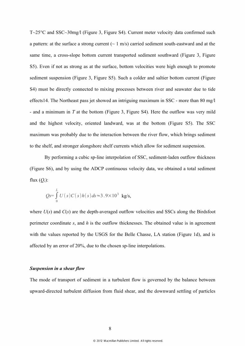
T~25°C and SSC~30mg/l (Figure 3, Figure S4). Current meter velocity data confirmed such

a pattern: at the surface a strong current (~ 1 m/s) carried sediment south-eastward and at the

same time, a cross-slope bottom current transported sediment southward (Figure 3, Figure

S5). Even if not as strong as at the surface, bottom velocities were high enough to promote

sediment suspension (Figure 3, Figure S5). Such a colder and saltier bottom current (Figure

S4) must be directly connected to mixing processes between river and seawater due to tide

effects14. The Northeast pass jet showed an intriguing maximum in SSC - more than 80 mg/l

- and a minimum in T at the bottom (Figure 3, Figure S4). Here the outflow was very mild

and the highest velocity, oriented landward, was at the bottom (Figure S5). The SSC

maximum was probably due to the interaction between the river flow, which brings sediment

to the shelf, and stronger alongshore shelf currents which allow for sediment suspension.

By performing a cubic sp-line interpolation of SSC, sediment-laden outflow thickness

(Figure S6), and by using the ADCP continuous velocity data, we obtained a total sediment

flux (Qs):

Qs=∫0

L

U ( s )C ( s )h( s )ds≈3 .9×103 kg/s,

where U(s) and C(s) are the depth-averaged outflow velocities and SSCs along the Birdsfoot

perimeter coordinate s, and h is the outflow thicknesses. The obtained value is in agreement

with the values reported by the USGS for the Belle Chasse, LA station (Figure 1d), and is

affected by an error of 20%, due to the chosen sp-line interpolations.

Suspension in a shear flow

The mode of transport of sediment in a turbulent flow is governed by the balance between

upward-directed turbulent diffusion from fluid shear, and the downward settling of particles

8


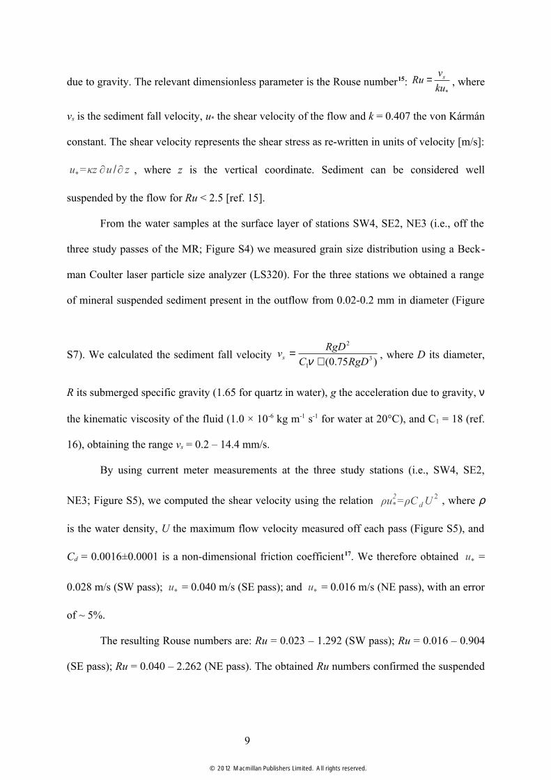
due to gravity. The relevant dimensionless parameter is the Rouse number15: *ku

vRu s= , where

vs is the sediment fall velocity, u* the shear velocity of the flow and k = 0.407 the von Kármán

constant. The shear velocity represents the shear stress as re-written in units of velocity [m/s]:

u* =κz ∂u /∂ z , where z is the vertical coordinate. Sediment can be considered well

suspended by the flow for Ru < 2.5 [ref. 15].

From the water samples at the surface layer of stations SW4, SE2, NE3 (i.e., off the

three study passes of the MR; Figure S4) we measured grain size distribution using a Beck-

man Coulter laser particle size analyzer (LS320). For the three stations we obtained a range

of mineral suspended sediment present in the outflow from 0.02-0.2 mm in diameter (Figure

S7). We calculated the sediment fall velocity )75.0( 3

1

2

RgDC

RgDvs +

=ν , where D its diameter,

R its submerged specific gravity (1.65 for quartz in water), g the acceleration due to gravity, ν

the kinematic viscosity of the fluid (1.0 × 10-6 kg m-1 s-1 for water at 20°C), and C1 = 18 (ref.

16), obtaining the range vs = 0.2 – 14.4 mm/s.

By using current meter measurements at the three study stations (i.e., SW4, SE2,

NE3; Figure S5), we computed the shear velocity using the relation ρu*2=ρC d U 2 , where ρ

is the water density, U the maximum flow velocity measured off each pass (Figure S5), and

Cd = 0.0016±0.0001 is a non-dimensional friction coefficient17. We therefore obtained u* =

0.028 m/s (SW pass); u* = 0.040 m/s (SE pass); and u* = 0.016 m/s (NE pass), with an error

of ~ 5%.

The resulting Rouse numbers are: Ru = 0.023 – 1.292 (SW pass); Ru = 0.016 – 0.904

(SE pass); Ru = 0.040 – 2.262 (NE pass). The obtained Ru numbers confirmed the suspended

9


load regime of the sediment-laden outflows, and in particular that the SW and SE passes had

well-suspended sediment, indicating strong jets that may have limited deposition.

The sediment-Potential Vorticity

We provide here the essential definitions and tools required to determine the sediment-

Potential Vorticity (PV) of a sediment-laden river plume and to understand its physical

meaning. The material presented here is based on Pedlosky18 and Falcini and Jerolmack19.

From (i) the continuity equation ∇⋅⃗u=−1ρ

dρdt

, where u⃗ is the velocity, ρ the water

density, p the pressure, and t the time; (ii) the Navier-Stokes equation

, where ω⃗=∇× u⃗ the relative flow

vorticity, 2Ω

the planetary vorticity, φ the force potential due to the gravity, F⃗ the ex-

ternal force per unit volume; and assuming that (iii) the SSC (c) within a sediment-laden jet

can be considered as a scalar fluid property not materially conserved, such that dcdt

=Ψ ,

where Ψ is a source/sink term for c, the Ertel20 PV theorem gives

ddt (

2 +ωΩ

ρ⋅∇ c)=2+ω⃗Ω ρ

∇ ρ×∇ p

ρ3

∇ cρ [∇×( F⃗

ρ )] , (S1)

where Π c=2+ω⃗Ω ρ

is the PV for suspended sediment. Equation (S1) provides a

mathematical framework for describing the offshore evolution of the MR: Π c is a pairing

between the jet vorticity due to the internal shearing and the gradient of SSC; it constitutes a

general parameter that describes the pertinent sediment and flow conditions of the river-

mouth plume.

10


It is worth noting that the definition of PV collects all the key features of a sediment-

laden spreading jet, where the vertical and horizontal shear velocity is coupled with the hori-

zontal and vertical distribution of suspended sediments19:

, (S2)

where we reasonably assumed that, at the local scale, the planetary vorticity is smaller than

the shear vorticity of the jet.

One can moreover assume that ∇ c⋅∇ ρ×∇ p≈0 if the density of a river outflow is

mainly driven by the suspended sediment. This makes (S1) more compact:

ddt

Π c=ω⃗ρ⋅∇ Ψ+

∇ cρ

⋅[∇×( F⃗ρ )] . (S3)

S3 shows that if a strong PV system (i.e., strong shear vorticity) input at the outlet of a river

remains conserved (i.e., 0=Π cdt

d), without losing sediment ( ∇Ψ=0 ) and in absence of

friction ( ∇×( F⃗ρ )=0 ), then the jet will propagate, conserving its shearing structure and

behaving like a self-sharpening filament19,21-26.

We estimated PV values at the Southwest, Southeast, and Northeast pass outlets (i.e.,

stations SW4, SE2, NE3; Figure 1, Figure S4, Figure S5), as well as the PV evolution along

the Southwest pass plume (i.e., transects SW, Pass 1, Pass 4; Figure 3, Figure S4 and Figure

S5), by scaling PV from equation (S2):

ρΠ c=( ∂v∂ x

−∂ u∂ y )∂ c

∂ z+

∂ u∂ z

∂ c∂ y

≈Uh

CW , (S4)

11


where U and C are the maximum values for the depth-averaged outflow velocities and SSCs,

h is the outflow thicknesses, and W the outflow width (Figure 3, Figure S5). PV values are

reported in Table S1. According to (S4), a high-PV system would represent a river plume

with a high sediment flux through a small cross-sectional area, a feature that seems to be in

agreement with the filament like plume observed for the MR at the Southwest pass.

Πc values along the Southwest pass outflow (SW4/SW, Pass1, and Pass 4 in Table S1)

lead to the conclusion that 0=Π cdt

d along this outflow. This demonstrates that PV is

approximately conserved, and thus the Southwest pass plume maintains its internal shearing,

delivering sediment far offshore. As discussed, a conserved PV is the necessary condition for

self-sharpening jet dynamics27,28, and justifies the ability of the MR to penetrate the coastal

current – which would otherwise deliver the sediment alongshore (Figure S8). On the

contrary, the high PV-conserved filament from the MR delivers sediment offshore and is

characterized by no (or very mild) lateral spreading.

3. Marsh Sediment Sampling

Potential sampling sites were pre-selected in each of four basins in coastal Louisiana

(Atchafalaya, Terrebonne, Barataria, and Mississippi River (“Birdsfoot”) Delta) using aerial

photography and maps. The majority of sites were selected based on proximity to long-term

monitoring stations (Coast-wide Referencing Monitoring System (CRMS)) maintained by the

State of Louisiana’s Office of Coastal Protection and Restoration

(http://lacoast.gov/crms_viewer/). Using information from the CRMS database and aerial

photography, we identified sites dominated by herbaceous vegetation (freshwater marshes in

12


http://lacoast.gov/crms_viewer/

the Atchafalaya and Birdsfoot basins and salt marshes in Barataria and Terrebonne basins).

A few additional sites were identified in areas without a CRMS station or where the site or

soil surface was inaccessible. From this pool of potential sites, 45 were randomly selected

for sampling. Sites were visited once in the early summer of 2011 on June 21, 22, 23 (Eastern

Terrebonne, Barataria, and Birdsfoot) and 27 (Atchafalaya and western Terrebonne).

Sites were accessed with a Bell 2063B Jet Ranger helicopter with fixed floats (allowing

marsh landings), which was positioned so that sampling would occur at a consistent distance

from a waterway (about 5 m). At each location, the soil surface was identified, and four soil

cores were collected with a piston corer (2 cm diameter x 15 cm length), which minimizes

vertical compression, and extruded onto a clean, flat surface. As a check for core

compression, a fifth core was collected with a “mini-McCauley” corer, which cuts a half-

section of a soil core in a horizontal plane against a stationary blade. In most cases, there was

a visually obvious surface layer of sediment of variable thickness but which was readily

distinguished as a recent deposit by the lack of plant roots and unconsolidated consistency.

Also, there was often a natural break in the soil core at the juncture between the surface

deposit and deeper layers, which were of a different colour, texture, and consistency. The

thickness of the surface layer for all five cores was measured and recorded; these five values

were averaged to provide a mean value for each sampling site. The four piston cores were

subsampled for further analysis. The upper layer of each core was carefully separated and

placed into a zip-lock bag; a segment (2 cm length) of the underlying material was also

collected and bagged separately. Samples of the surface water and pore water were collected

at each site with a sipper device and salinity was measured in the field with a refractometer.

The dominant vegetation at each site was identified to species and recorded.

At the laboratory, half of the soil samples (n = 2 cores x 2 depths per site) were weighed

wet, dried in an oven at 60 °C to constant mass, and reweighed. Dry bulk density was

13


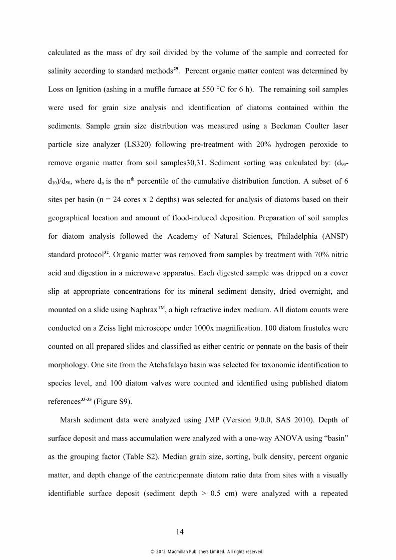
calculated as the mass of dry soil divided by the volume of the sample and corrected for

salinity according to standard methods29. Percent organic matter content was determined by

Loss on Ignition (ashing in a muffle furnace at 550 °C for 6 h). The remaining soil samples

were used for grain size analysis and identification of diatoms contained within the

sediments. Sample grain size distribution was measured using a Beckman Coulter laser

particle size analyzer (LS320) following pre-treatment with 20% hydrogen peroxide to

remove organic matter from soil samples30,31. Sediment sorting was calculated by: (d90-

d10)/d50, where dn is the nth percentile of the cumulative distribution function. A subset of 6

sites per basin (n = 24 cores x 2 depths) was selected for analysis of diatoms based on their

geographical location and amount of flood-induced deposition. Preparation of soil samples

for diatom analysis followed the Academy of Natural Sciences, Philadelphia (ANSP)

standard protocol32. Organic matter was removed from samples by treatment with 70% nitric

acid and digestion in a microwave apparatus. Each digested sample was dripped on a cover

slip at appropriate concentrations for its mineral sediment density, dried overnight, and

mounted on a slide using NaphraxTM, a high refractive index medium. All diatom counts were

conducted on a Zeiss light microscope under 1000x magnification. 100 diatom frustules were

counted on all prepared slides and classified as either centric or pennate on the basis of their

morphology. One site from the Atchafalaya basin was selected for taxonomic identification to

species level, and 100 diatom valves were counted and identified using published diatom

references33-35 (Figure S9).

Marsh sediment data were analyzed using JMP (Version 9.0.0, SAS 2010). Depth of

surface deposit and mass accumulation were analyzed with a one-way ANOVA using “basin”

as the grouping factor (Table S2). Median grain size, sorting, bulk density, percent organic

matter, and depth change of the centric:pennate diatom ratio data from sites with a visually

identifiable surface deposit (sediment depth > 0.5 cm) were analyzed with a repeated

14


measures ANOVA using basin as the grouping factor and soil depth (upper, lower) as the

repeated measure (Table S3). Data were log-transformed where necessary to meet

assumptions of ANOVA (equal variance, normality). In a few cases, data outliers were

identified (Mahalanobis distance) and excluded from analysis. When a significant effect was

found, differences among multiple means were identified with Tukey’s Honestly Significant

Difference.

Tables

Table S1. MR plume values for the estimation of the bulk PV (ρΠc): maximum values for the depth-averaged outflow velocity (U) and SSC (C); and outflow thicknesses (h) and outflow width (W). See Figure 1, Figure 3, Figure S4, and Figure S5.Station/Transect U [m/s] C[mg/l] h[m] W[m×103] ρΠc[kg m-4s-1]SW4/SW 1.4 80 3 1.5 2.49×10-5

SE2 1.0 50 2 1 2.50×10-5

NE3 0.4 100 4 1 1.00×10-5

Pass 1 1.4 60 2.5 1.5 2.24×10-5

Pass 4 1.2 40 2 1.5 2.14×10-5

Table S2. Summary of statistical analyses of marsh sedimentation data. One-way Analysis of Variance (ANOVA) using basin as the grouping factor was used to analyze porewater salinity, flood sediment depth and accumulation (depth x bulk density). Significant differences among means for the main effect of basin (Tukey’s Honestly Significant Difference) are indicated by different letters.

Basin n Marsh TypePorewater

Salinity (‰)

s.e.Sediment

Depth (cm)

s.e.Sediment

Accumulation (g cm-2)

s.e.

Atchafalaya 14 Freshwater <1a <1 2.6a 0.7 1.61a 0.48 Barataria 8 Saline 23b 3 0.8ab 0.2 0.32ab 0.10

Birdsfoot 9 Freshwater <1a <1 1.4ab 0.3 1.14ab 0.39

Terrebonne 14 Saline 21b 3 0.7b 0.2 0.41b 0.08 Overall Mean

45 10.7 1.9 1.5 0.3 0.91 0.19

Probability > F <0.0001 0.0194 0.017

Table S3. Summary of statistical analyses of marsh sediment characteristic data. Mean and standard error (s.e.) are listed only for sites with a distinct surface sediment layer (sediment depth > 0.5 cm). Repeated measures ANOVA was used to measure bulk density, percent (%) organic matter, mean grain size, sorting and centric:pennate (C:P) ratio. Depth (upper (flood), lower (pre-flood)) was the repeated measure and basin was the grouping factor, where the

15


interaction term indicates a different pattern across basins in depth variation. Significant differences among means for the main effect of basin (Tukey’s Honestly Significant Difference) are indicated by different letters. Data outliers identified by Mahalanaobis Distance (based on upper x lower correlation) were excluded from analysis of some variables: bulk density (2 outliers), organic matter (2 outliers), median grain size (3 outliers), sorting (3 outliers), and centric:pennate ratio (3 outliers).

Basin nBulk

Density (g cm-3)

s.e.Organic Matter

(%)s.e.

Median Grain

Size (µm)s.e. Sorting* s.e.

C:P ratio†

s.e.

Atchafalaya 9 0.65 0.10 6a 1 11.4ab 2.5 3.9 0.6 0.73 0.23Barataria 5 0.39 0.12 18b 2 21.9a 3.2 5.2 0.7 0.47 0.23Birdsfoot 7 0.68 0.11 7a 1 13.5ab 3.2 4.5 0.8 1.36 0.21Terrebonne 7 0.63 0.10 11a 1 9.4b 2.7 5 0.6 0.59 0.23OverallMean

29 0.60 0.05 10 1 13.4 1.6 4.6 0.3 0.6 0.05

Source of Variation Probability of >F; ‘ns’ indicates test was not significant at p<0.05 levelBasin ns 0.0002 0.0369 ns nsDepth 0.0011 0.0435 ns 0.0360 0.006Basin x Depth ns ns ns ns 0.009

*Sorting was calculated by (d90-d10)/d50, where dn is nth percentile of cumulative distribution function.† C:P = centric:pennate ratio for a subset of n = 6 sites per basin.

16


References

1. http://www.mvn.usace.army.mil/bcarre/morganza.asp.

2. CBS News/Associated Press. http://www.cbsnews.com/stories/ 2011/05/14/national/

main20062948.shtml.

3. The Watchers. http://thewatchers.adorraeli.com/2011/05/14/morganza-spillway-about-to-

open/.

4. The Associated Press. http://www.nola.com/environment/index.ssf/2011/06/

last_gates_at_bonnet_carre_spi.html.

5. Kroes, D. The Effect of the opening of the Morganza Spillway on the Flow Patterns and

Sediment Distribution within the Swamps of the Atchafalaya River Basin. AGU- Fall

Meeting 2011, B24D-02.

6. http://www.oso.noaa.gov/poes/

7. http://www.esl.lsu.edu/home/

8. http://modis.gsfc.nasa.gov/

9. http://imars.marine.usf.edu/

10. Rodríguez-Guzmán, V. & Gilbes-Santaella, F. Using MODIS 250 m imagery to estimate

total suspended solids in a Tropical Open Bay. International Journal of Systems

Applications, Engineering & Development. 3, 36–44 (2009)

11. Guillén, J. et al. Field calibration of optical sensors for measuring suspended sediment

concentration in the western Mediterranean. Scientia Marina 64, 427-435 (2000)

12. Rego, J., Meselhe, E., Stronach, J. & Habib, E. Numerical Modeling of the Mississippi-

Atchafalaya Rivers' Sediment Transport and Fate: Considerations for Diversion

Scenarios. J. Coastal Res. 26, 212-229 (2010).

13. Yuan J., Miller R. L., Powell, R. T. & Dagg M. J. Storm-induced injection of the

Mississippi River plume into the open Gulf of Mexico. Geophys. Res. Lett. 31 (2004).

14. Li, C. et al. Summertime tidal flushing of Barataria Bay: Transports of water and

suspended sediments. J. Geophys. Res. 116, C04009 (2011)

15. Bagnold, R. An approach to the sediment transport problem from general physics, U.S.

Geol. Surv. Prof. Pap. 422-I (1966).

16. Ferguson R. I. & Church, M. A Simple Universal Equation for Grain Settling Velocity. J.

of Sediment. Res. 74, 933-937 (2004).

17


http://imars.marine.usf.edu/

17. Rowland, J. C., Dietrich, W. E. & Stacey, M. T. Morphodynamics of subaqueous levee

formation: Insights into river mouth morphologies arising from experiments, J. Geophys.

Res. 115, F04007 (2010).

18. Pedlosky, J. Geophysical Fluid Dynamics, Springer-Verlag, New York (1979).

19. Falcini, F. & Jerolmack, D.J. A potential vorticity theory for the formation of elongate

channels in river deltas and lakes. J. Geophys. Res. 115, F04038 (2010).

20. Ertel, H. Ein neuer hydrodynamischer Wirbelsatz, Meteorol. Z. 59, 277–281 (1942).

21. Hu, C. et al. Mississippi River water in the Florida Straits and in the Gulf Stream off

Georgia in summer 2004, Geophys. Res. Lett. 32, L14606 (2005).

22. Shi, W. & Wang, M. Satellite observations of flood-driven Mississippi River plume in the

spring of 2008. Geophys. Res. Lett. 36, L07607 (2009).

23. Peckham, S. D. A new method for estimating suspended sediment concentrations and

deposition rates from satellite imagery based on the physics of plumes. Comput. Geosci.

34, 1198-1222 (2008).

24. Walker, N. D., Rouse Jr., L. J., Fargion, G. S. & Biggs, D. C. The Great Flood of summer

1993: Mississippi River discharge studied, Eos Trans. AGU 75, 409 (1994).

25. Bignami, F. et al. On the dynamics of surface cold filaments in the Mediterranean Sea, J.

Mar. Res. 74, 429-442 (2008).

26. Holland, W. R. On the wind-driven circulation in an ocean with bottom topography,

Tellus 19, 582-600 (1967).

27. Wood, R. B. & McIntyre, M. E. A general theorem on angular-momentum changes due to

potential vorticity mixing and on potential-energy changes due to buoyancy mixing. J.

Atmos. Sci. 67, 1261-1274 (2010).

28. Dritschel, D. G. & Scott, R. K. Jet sharpening by turbulent mixing. Phil. Trans. R. Soc. A

369, 754-770 (2011).

29. Noorany, I. Phase relations in marine soils. Journal of Geotechnical Engineering 110,

539-543 (1984).

30. Allen, J. R. L. & Thornley, D. M. Laser granulometry of Holocene estuarine silts: effects

of hydrogen peroxide treatment. Holocene 14, 290-295 (2004).

31. Hawkes, A. D. et al. Sediments deposited by the 2004 Indian Ocean Tsunami along the

Malaysia-Thailand Peninsula. Mar Geol 242, 169-190 (2007).

32. Charles, D. F., Knowles, C. & Davis, R. Protocols for the analysis of algal samples

collected as part of the U.S. Geological Survey National Water-Quality Assessment

Program. (The Academy of Natural Sciences, Philadelphia, 2002).

18


33. Lange-Bertalot, H. Diatoms of Europe: Diatoms of the European inland waters and

comparable habitats. Vol. 3 (Koeltz Scientific Books, 2002).

34. Witkowski, A., Lange-Bertalot, H. & Metzeltin, D. Diatom flora of marine coasts. Vol.

07: Diversity - Taxonomy - Identification (Koeltz Scientific Books, 2000).

35. Krammer, K. & Lange-Bertalot, H. Bacillariophyceae. Band 2/1-4 (Gustav Fischer

Verlag, 1991).

19


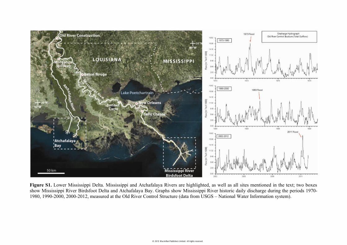
Figure S1. Lower Mississippi Delta. Mississippi and Atchafalaya Rivers are highlighted, as well as all sites mentioned in the text; two boxes show Mississippi River Birdsfoot Delta and Atchafalaya Bay. Graphs show Mississippi River historic daily discharge during the periods 1970-1980, 1990-2000, 2000-2012, measured at the Old River Control Structure (data from USGS – National Water Information system).


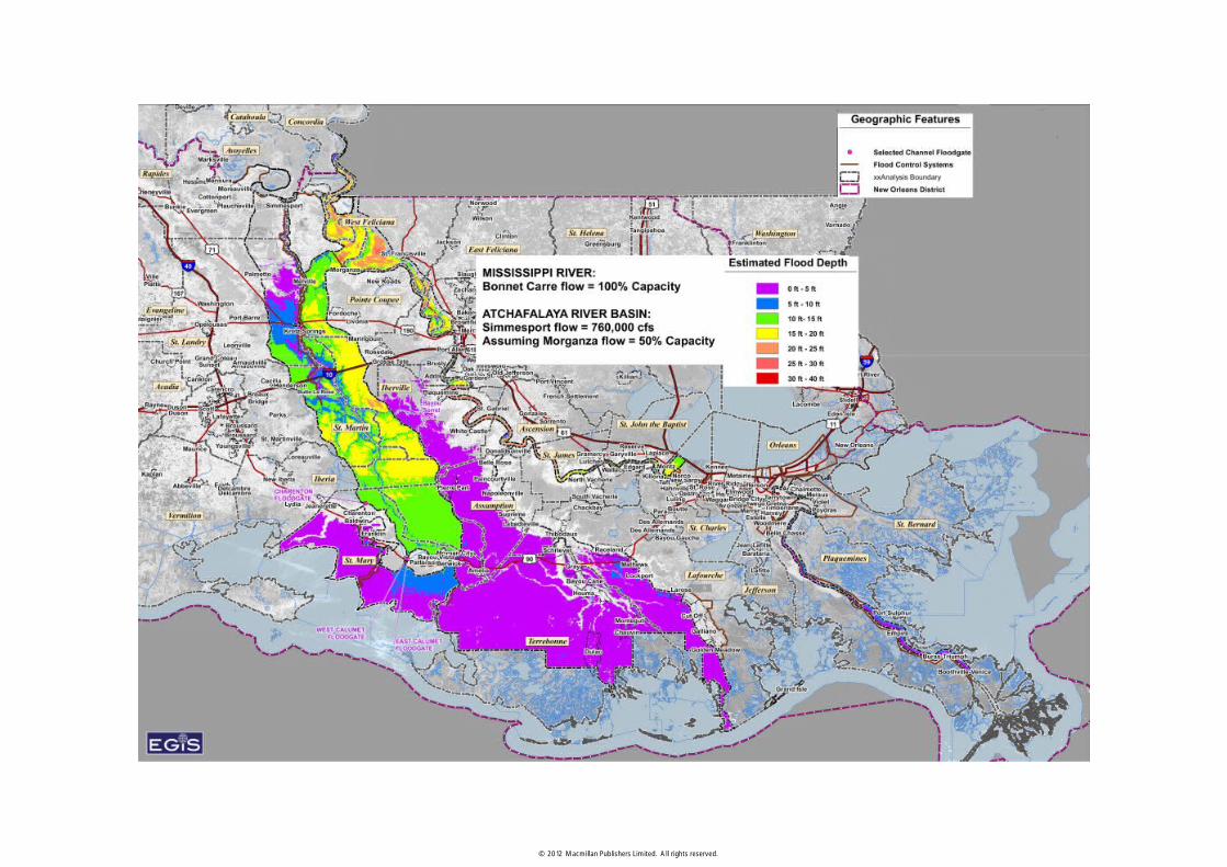
Figure S2. Map of projected inundation of the Atchafalaya Basin resulting from opening of the Morganza Floodway, generated for flood preparation by United States Army Corps of Engineers (http://www.mvn.usace.army.mil/news/view.asp?ID=461). The inundation pattern suggests that some Atchafalaya Basin wetland sedimentation likely resulted from direct deposition by flood waters, in addition to plume-derived sedimentation from the mouth. On the other hand, the Birdsfoot Delta and neighbouring basins were not significantly inundated by overland flow, limiting direct deposition of sediment from flood waters; plume-derived sedimentation likely dominated in areas outside of the Atchafalaya Basin.


http://www.mvn.usace.army.mil/news/view.asp?ID=461

Figure S3. Mississippi River (MR) and Atchafalaya River (AR) plume patterns seen from sea surface temperature (SST) data. a, Time-averaged SST reveals the position of the Southwest pass MR plume during the 2011 flood (5 May – 5 June); white zones indicate the dominant position of the plume during that time. b, Standard deviation related to the average on panel a; the narrow, dark zone off the Southwest pass highlights the low variability of the plume position in that region. Image statistical analysis was carried out from SST maps using ImageJ Software. c, d, NOVA/AHRR SST along the Atchafalaya Bay and the Birdsfoot Delta, respectively, on June 1, 2011 (data processed by the Earth Scan Lab – Coastal Studies Institute, Louisiana State University).


Figure S4. Hydrographic transects around the MR Birdsfoot Delta on June 1, 2011. a, Bathymetric map of the area, with hydrographic/ suspended sediment station and ADCP transects performed during the boat survey (see text); the large scale transect A-A’ around the Delta is highlighted in grey. b, Salinity cross-section profile around the Birdsfoot Delta: three main freshwater plumes can be observed at ~ 20, 80, and 150 km of distance from the beginning of the transect. c, Temperature cross-section profile around the Birdsfoot Delta: cold jet from the Southwest pass can be observed at ~ 20 km of distance from the beginning of the transect; the two bottom cold waters at ~80 and 150 km are likely associated with hyperpicnal flows coming from the Southeast and Northeast passes, respectively.


Figure S5. Current meter measurements off the MR Birdsfoot Delta on June 1, 2011. a, Velocity profiles (magnitude and stick vectors) off the Southwest, Southeast, and Northeast passes (from left to right); the bottom current directions differ from the surface, indicating a baroclinic structure due to the river dynamics. b, Continuous current meter data along the transects SW, Pass 1 and Pass 4, from left to right (see Figure S4); blue colours (>80 cm/s) are associated with the Southwest pass jet, which conserved PV and momentum and thus maintained its coherent structure (see text).


Figure S6. Analytic interpolations for the outflow characteristics of the Southwest, Southeast, and Northeast outflow (respectively at ~20, 100, and 150 km of distance from the beginning of the transect A-A’, see Figure S4). a, Cubic sp-line interpolation of suspended sediment (C) and outflow depths (h). b, Gaussian interpolation of the outflow velocities. Dots indicate the related measured values around the Birdsfoot Delta and off each pass. The interpolation of flow velocity off the SW pass is constrained by the ADCP data of transect SW. The width of the Gaussian interpolation for the passes SE and NE is obtained from the channel widths.


Figure S7. Example grain size distribution, from a surface sample at the station SW (see Figure S4). The analysis was performed using a Beckman Coulter laser particle size analyzer (LS320).


Figure S8. Nowcast results showing superficial ocean current (white vectors), from South Atlantic Bight and GoM Circulation Model (SABGOM; developed, operated and maintained by Ocean Observing and Modeling Group of Department of Marine, Earth and Atmospheric Sciences, NCSU) superimposed on MODIS ocean colour images (data processed by Institute of Marine Remote Sensing, USF) for two representative days of the flood (31 May and 2 June, 2011). Both maps show that the Mississippi River sediment plume penetrated the coastal current, despite large near-shore drift velocities (up to 1 m/s), and delivered sediment far offshore. The Atchafalaya plume, however, remained completely contained within the coastal current; note that the plume followed the shift in coastal current from west to south, indicating that the coastal current dominated Atchafalaya plume dynamics.


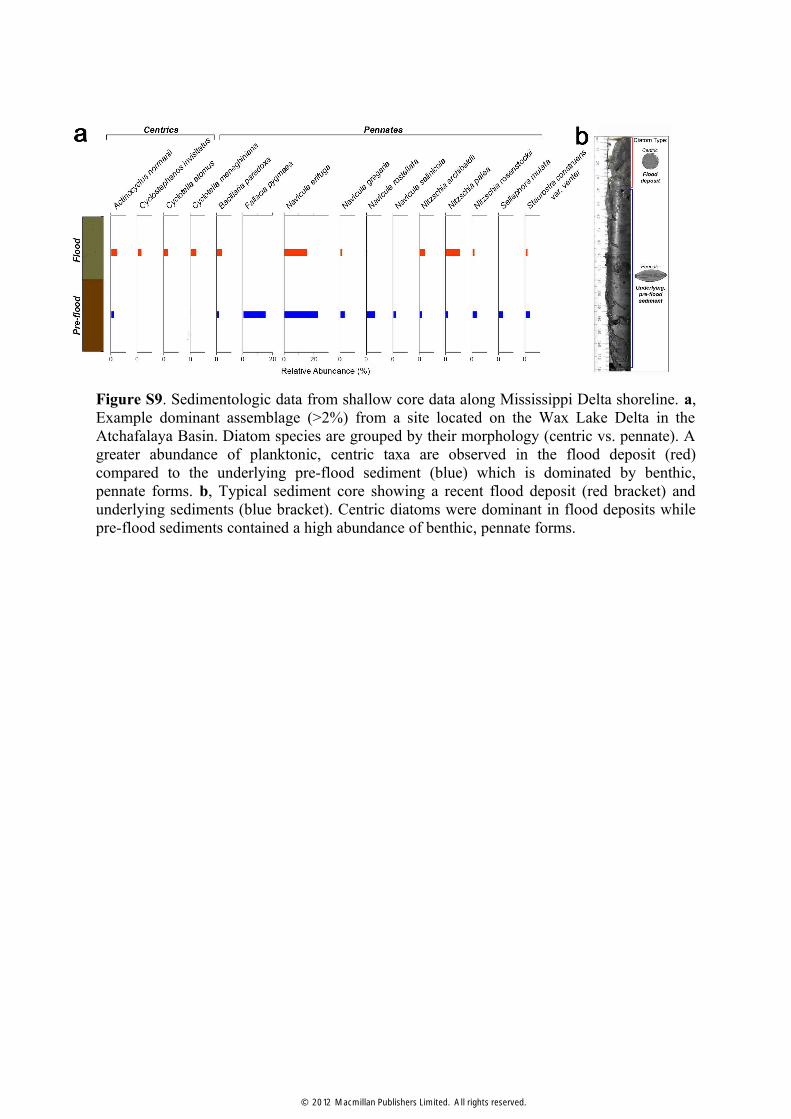
Figure S9. Sedimentologic data from shallow core data along Mississippi Delta shoreline. a, Example dominant assemblage (>2%) from a site located on the Wax Lake Delta in the Atchafalaya Basin. Diatom species are grouped by their morphology (centric vs. pennate). A greater abundance of planktonic, centric taxa are observed in the flood deposit (red) compared to the underlying pre-flood sediment (blue) which is dominated by benthic, pennate forms. b, Typical sediment core showing a recent flood deposit (red bracket) and underlying sediments (blue bracket). Centric diatoms were dominant in flood deposits while pre-flood sediments contained a high abundance of benthic, pennate forms.


supplementary information supplementary information … · recorders and manual measurements at...

Documents