supplementary information - media.nature.com · cut using a disposable stainless steel dissection...

Supplementary Methods

Supplementary Methods 1

1. Sample Processing Overview 3 2. Tissue Collection and Processing 4

a. Postmortem Tissue Acquisition and Screening 4 b. Initial Tissue Dissection and Freezing 6 c. Large Format Sectioning and Blockface Imaging 7 d. Slab Partitioning 7 e. Processing and Sectioning of 2x3 Blocks 8 f. Microarray Sample Collection by Macrodissection or

Laser Microdissection (LMD) 10 i. Manual Macrodissection 10 ii. LMD 11

g. RNA Isolation 12 i. RNA Isolation from Macrodissected Tissue Samples 12 ii. RNA Isolation from LMD Dissected Tissue Samples 13

h. Sample Preparation for Microarray Analysis 14 3. Data Generation 15

a. Magnetic Resonance Imaging 15 b. Histological Stains 15

i. Hematoxylin and Eosin (H&E) 16 ii. Nissl Stain 16 iii. Modified Bielschowski Silver Stain 16 iv. SMI‐32 Immunohistochemistry 17 v. In Situ Hybridization (ISH) 17

c. Microarray Data Generation 17 4. Data Processing 18

a. Microarray Data Processing 18 i. Initial Data Quality Control (QC) 18 ii. Normalization within a Single Brain 20 iii. Normalization across Multiple Brains 22

b. Digital Imaging and Processing of Histologically Stained Sections 22 c. MR Image Processing 22 d. Anatomic Mapping and Visualization 22

5. QC and Scientific Quality Assessment 24


1. Construction of Landscape Plot and Visualization 27 2. Data Processing for Weighted Gene Coexpression Network Analyses 27

a. Network Formation and Module Characterization 27 b. Comparative Analyses Accompanying WGCNA 28

3. Construction of Differential Correlograms and Clustering 29

WWW.NATURE.COM/NATURE | 1

SUPPLEMENTARY INFORMATIONdoi:10.1038/nature11405


1. Computation of Regionally Enriched Marker Genes 30 2. Cortical Analysis and Reconstruction 30 3. Least Squares Fitting in 3‐dimensions (3D) with Respect to Translation,

Rotation, and Scaling 30 4. Quaternions 32

References 36


SUPPLEMENTARY INFORMATIONRESEARCHdoi:10.1038/nature11405


Sample Processing Overview

The central challenge to the creation of an atlas of the entire human brain was the development of a process that enabled identification, delineation, and sampling of specific anatomic structures for microarray analysis, and that also allowed for the mapping of this sampling and resulting data back into three‐dimensional neuroanatomic space. The process involved multiple brain and tissue subdivision steps, with collection of anatomic and histological information at each partitioning level, where the resolution of the anatomic and histological information became higher as the tissue became further subdivided, ultimately resulting in delineation and dissection of small tissue samples for microarray analysis. A schematic of this process is shown in Figure 1. The steps were as follows:

1. Initial tissue collection and processing occurred at independent tissue banks or tissue repositories, and resulted in fresh frozen tissue slabs shipped to the Allen Institute for further processing.

2. After successful screening and QC of the tissue, a limited set of large format histology data was collected from each tissue slab with a 4.65 µm/pixel digital image resolution. A minimum specified amount of tissue in each slab was saved for the next processing step.

3. Each tissue slab was then subdivided into smaller tissue blocks categorized according to whether they contained primarily cortical or subcortical brain structures. These tissue blocks were sectioned for histology data with a final digital image resolution of 1 µm/pixel. If the blocks contained subcortical structures, additional sections were collected onto membrane slides that would allow LMD of these structures. A minimum specified amount of tissue in each block was saved for the next processing step.

4. Anatomically defined samples were collected for microarray analysis by either manual macrodissection of the remaining tissue from each block (cortical and some subcortical structures) or by laser microdissection (subcortical areas).

5. Tissue samples collected for microarray analysis were processed for RNA isolation, quantification, and normalization.

6. RNA samples that passed quality control metrics were sent for microarray analysis to an independent service company, Beckman Coulter Genomics (Morrisville, NC).

7. Data returned by Beckman Coulter Genomics were reviewed against quality control criteria, normalized and analyzed prior to inclusion in the Allen Human Brain Atlas dataset.

Throughout the process described above, anatomic data (MR, blockface images, and histology) were annotated to provide the information necessary to collect anatomically defined samples for microarray that also represented all structures from the human brain. Overall, the goal was to collect approximately 1,000 samples from each brain, representing all structures within the brain in approximate proportion to the volumetric representation of each cortical, subcortical, cerebellar and brainstem structure.

The following descriptions are divided into three main sections:

• Tissue Collection and Processing: provides information about tissue acquisition and screening, specific methods and anatomic criteria used to section and subdivide tissue, including sampling for microarray, and methods for RNA isolation and processing;



• Data Generation: provides specific methods for MR imaging, histological staining, and microarray experimental design and execution;

• Data Processing: describes processing steps required after data generation to include integrated data modalities in the online resource. This includes digital imaging of histological data, microarray data quality control and processing, and methods for anatomic visualization and mapping.

Figure 1. Process schematic of primary steps in the creation of the whole brain microarray survey of the Allen Human Brain Atlas. LIMS is the Laboratory Information Management System in which all data are tracked and processed for online presentation of data.

TISSUE COLLECTION AND PROCESSING

Postmortem Tissue Acquisition and Screening

Postmortem brains from men and women between 18 and 68 years of age, with no known neuropsychiatric or neuropathological history (‘control’ cases) were eligible for inclusion in the Atlas. Consent from next‐of‐kin was obtained in all cases. A screening process was employed to validate, as much as possible, a ‘control’ diagnosis, as well as to qualify the tissue for cytoarchitectural integrity and acceptable RNA quality. In addition to evidence of known history of neuropathological or neuropsychiatric disease, cases with long‐term illnesses or events that resulted in hypoxic conditions lasting more than an hour were also excluded. Recent literature indicates that hypoxia is one primary contributor to detrimental effects on RNA quality1,2. As a safety precaution, a serology screen was performed to exclude cases with Hepatitis B, Hepatitis C, or HIV‐1/HIV‐2 (ViroMed, Minnetonka, MN). Blood samples from each case were submitted for toxicology screening (NMS Labs, Willow Grove, PA) to determine presence of medications that might indicate neuropathology or neuropsychiatric disorder, including substance abuse or addiction. Gross neuropathology reports were provided by neuroradiologists based on MR data. Microneuropathology assessment was performed by a pathology consultant who viewed selected large format tissue sections stained with hematoxylin‐eosin (H&E),



thionin‐based Nissl stain, or silver to determine: (1) presence of local ischemic events; (2) evidence of senile plaques or neurofibrillary tangles; or (3) other cytoarchitectural abnormalities. In each case, the selected tissue sections targeted specific regions in which these events or phenomena were likely to occur (see Table 1). All screening and validation data were reviewed by a Case Review Committee (CRC) consisting of Allen Institute staff and external advisors with varying expertise in imaging, genetics, and neuroanatomy. Figure 2 shows the general timing of screening information availability and CRC decision points.

Table 1. Anatomic regions routinely assessed for microneuropathology. Anatomic Regions for Microneuropathology Assessment Section Orientation Slide Size

At level of amygdala Coronal 6x8

Frontal lobe at level of anterior temporal pole Coronal 6x8

Dorsal half of substantia nigra/posterior hippocampus Coronal 6x8

Posterior parietal lobe Coronal 6x8

Occipital lobe (towards occipital pole) Coronal 6x8

Cerebellum, lateral hemisphere, right Sagittal 6x8

Cerebellum, lateral hemisphere, left Sagittal 6x8



Figure 2. Timeline for availability of screening and quality control data used to qualify tissue for further processing for microarray. The Case Review Committee (CRC) was notified when data became available and met as needed depending on the complexity of data received.

Initial Tissue Dissection and Freezing

Initial collection, dissection, and freezing of whole brain were performed at the NICHD Brain and Tissue Bank at the University of Maryland, Baltimore, or at the Functional Genomics Laboratory at the Department of Psychiatry and Human Behavior, University of California, Irvine. A multipart dissection and processing protocol was utilized, resulting in fresh frozen tissue comprising: (1) full cerebral slabs cut in coronal orientation; (2) cerebellar slabs cut in sagittal orientation; and (3) whole brainstem. Slab thicknesses ranged from approximately 0.5 to 1 cm at the time of dissection. This slabbing scheme was established to acquire the most recognizable histology results to define anatomic regions for microarray analysis.

The dissection and freezing protocol involved a number of detailed steps. Briefly, upon completion of MR imaging (see ‘DATA GENERATION ‐ Magnetic Resonance Imaging’ below), the whole brain was chilled to approximately 4°C and dissected by separating the cerebellum and brainstem from the cerebrum. A small sample of the frontal pole was taken for pH measurement. The brainstem was then removed from the cerebellum with a transverse cut just dorsal to the pons. The brainstem was immediately placed on a Teflon freezing plate and frozen slowly to avoid cracking.

In the meantime, the cerebrum and cerebellum were prepared for dissection by encasing each structure separately in alginate (Cavex BV, Haarlem, The Netherlands) and chilling the alginate to just above freezing. Typically used for dental impressions, alginate was used here to preserve overall brain shape during the slabbing process. Liquid alginate was prepared by combining 250 g of alginate powder with 2 l of ultra pure water in a blender. The cerebellum or cerebrum was placed in a structure‐specific molded



cavity created with a brain model (Global Technologies, Sunrise, FL) partially submerged in liquid alginate. Once the alginate hardened the tissue was placed in the molded cavity in place of the model, covered with additional liquid alginate to completely encase the tissue and placed in 4°C or ‐80°C to cool. Once the alginate cooled sufficiently and the tissue became firmer, the cerebellum and cerebrum were cut into approximately 0.5‐ to 1‐cm‐thick slabs using a metal apparatus custom‐designed to ensure consistency of slab thickness. The apparatus included a sliding platform on which the alginate‐encased tissue was placed. For each slab, the platform was advanced in 0.5 or 1 cm increments and tissue was cut using a disposable stainless steel dissection knife (Mopec, Oak Park, MI). A knife guide affixed to the apparatus was used to control the path of the knife through the tissue and alginate. Tissue slabs were frozen almost immediately after they were cut by controlled immersion in a bath of dry ice and isopentane. Each slab was placed between two metal plates during freezing to maintain flat surfaces in the cutting plane. Each frozen slab was stored separately in a labeled vacuum‐sealed plastic bag at ‐80°C prior to shipping to the Allen Institute.

Frozen slabs were individually placed in 6x8 inches padded envelopes to guard against breakage, snugly packed in a polystyrene foam box containing dry ice and shipped via overnight courier to the Allen Institute. Upon receipt, slabs were photographed and inspected for uniformity of slab thickness, anatomic plane of slabbing, and possible damage such as cracks or breaks in the tissue. Following inspection, slabs were stored at ‐80°C until future use. Photographic images taken at the time of slabbing and tissue receipt were reviewed to assess gross brain morphology, and symmetry and consistency of the cutting plane. Issues were documented for review and discussion by the CRC.

Large Format Sectioning and Blockface Imaging

In preparation for large format sectioning, frozen coronal and sagittal slabs were embedded and surrounded in mounting medium (OCT or CMC), resulting in flat frozen rectangular slabs comprising mounting media surrounding centrally embedded tissue. This process was done on a metal platform set on dry ice so that the tissue stayed frozen at all times. Care was taken to level the metal platform and tissue as much as possible. Aluminum bars were used as a frame to contain the media when first applied around the tissue and were removed as soon as the edges of the media solidified. Once all of the media solidified, embedded slabs were stored at ‐20°C for at least 24 hours prior to sectioning. Large format full coronal and sagittal tissue sections were placed on large glass slides (6x8) for histological staining using a tape transfer method. Briefly, an embedded slab was mounted using OCT on the leveled chuck of a Reichert‐Jung Cryo‐Polycut (‐18°C to ‐20°C at the chuck) and sectioned with a wedge‐shaped steel blade (Leica, Wetzlar, Germany) until the top layer of mounting media was removed. Coronally cut cerebral slabs were mounted with the anterior surface facing up while sagitally cut cerebellar slabs were mounted with the anatomic left‐facing surface facing up. When a full tissue section was achieved, blockface imaging and collection of tissue sections for histology commenced. When it was not possible to obtain a full tissue section due to inconsistencies in tissue flatness, sections were taken at a tissue depth that allowed further processing of the slab for microarray sampling. Tissue sections for histology (25 or 50 µm thick) were placed on chilled (‐11°C to ‐13°C) glass slides coated with Solution A and Solution B (Instrumedics, Ann Arbor, MI) pretreatment and adhesive, respectively, using Macro‐Tape‐Transfer System (Instrumedics). Tape flags cut to be slightly longer than the embedded slab were adhered to the tissue surface and smoothed with a brush to eliminate air bubbles. The tape was used to pick up the tissue section after it was cut at approximately half‐speed (setting 10 on a 1 to 20



scale). The flag and tissue were then placed tissue side down onto the surface of a glass slide. A brush was used to smooth the tissue and eliminate air bubbles. Tissue was adhered to the slide using a UV polymerizer placed over the glass slide for approximately 2 x 30 s flashes. After removal of the tape, tissue slides were allowed to dry at room temperature and were subsequently stored at ‐20°C until histological staining. Blockface digital images were obtained after every histology tissue section was collected using a Canon EOS Rebel XSi camera with a Canon EF 50 mm macrolens and Canon MT‐24EX flash. The camera was permanently mounted approximately two feet above the chuck and centered above the chuck’s stopping point. Blockface images were used for annotation of anatomic regions and for mapping histological and gene expression information into 3D MR image space.

Slab Partitioning

Slab partitioning was done after large format sectioning to subdivide full coronal or full sagittal tissue slabs into pieces that could be further processed for histology data and microarray sampling using smaller (2x3 inches) microscope slides. These smaller sizes allowed the use of existing high‐throughput histology equipment and processes for increased rate of data generation and higher image resolution of histological data relative to processes for 6x8‐inch data generation.

Each slab was partitioned on a flat metal dissection table housed in a modified temperature‐controlled cryostat (‐15°C). The slab was placed on a pre‐chilled Teflon dissection board and subdivided using a steel blocking blade (Brain Research Laboratories, Newton, MA) and disposable sterile surgical blades (#11, #15, and #21, Feather Safety Razor Company, Osaka, Japan). A partitioning diagram was used to guide the placement of each cut into the slab. This diagram was drawn on the last blockface image collected for each slab, with cutting lines placed so that: (1) all resulting pieces fit onto 2x3 slides; (2) cuts through cortex were perpendicular through all cortical layers (i.e., there were no transverse cuts separating cortical layers); (3) each 2x3 block contained mostly cortical or mostly subcortical structures; (4) subcortical structures were kept intact as much as possible (cuts through the putamen were almost always necessary); and (5) sufficient tissue support was maintained around periventricular structures in order to minimize tissue warping during processing. Each piece was categorized into one of three subtypes for future processing based on being either (1) primarily cortical (cx), (2) subcortical with small or oddly shaped structures (s1), or (3) subcortical with large structures (s2). A representative partitioning diagram (Figure 3A) shows cutting lines used for a slab with all cx blocks and associated grid

Figure 3. Representative slab partitioning diagram (A) andannotated Nissl image (B). The partitioning diagram (A) shows cx block designations and x, y, z coordinates within the slab to assist inlater reconstruction efforts. The Nissl image shows cortical delineations of major gyri labeled according to the Atlas ontology.Red arrows point to corresponding anatomic features in the Nisslimages relative to the partitioning diagram. The yellow circleindicates a macrodissection site outlined on the Nissl image as asquare shape. Multiple macrodissection sites can be seen in B.

A B



coordinates (x, y, z) for each piece in that slab. Grid coordinates were later used for reconstruction of 2x3 pieces into a full slab (see ‘Anatomic Mapping and Visualization’). After subdivision, the full slab was reassembled and an image was taken and saved. Each resulting block was stored at ‐80°C in a separate plastic storage bag with a unique identifying label until sectioning. The entire partitioning process was video recorded in case it became necessary to track down inadvertent sample swaps at a later date.

The brainstem did not require subdividing in this same manner because transverse sections already fit onto 2 x 3 slides. However, the brainstem was subdivided in the transverse plane by cutting below the pons to create blocks less than 3 cm in length to be compatible with maximum clearance in the cryostat.

Processing and Sectioning of 2x3 Blocks

Slab partitioning resulted in 3 primary tissue type blocks based on anatomic areas contained within each block and the type of dissection required to collect microarray samples of the desired structures at the desired resolution. Cortical (cx) blocks contained primarily cortical regions for which manual macrodissections were done to collect tissue samples for microarray analysis. Subcortical s1 blocks contained primarily subcortical regions with oddly shaped structures or small substructures that required dissection by LMD. For example, s1 blocks contained structures such as amygdala, hypothalamus and thalamus. Subcortical s2 blocks contained primarily subcortical regions that were designated for manual macrodissection, such as caudate, putamen and globus pallidus. Tissue sections were collected from each block for histological staining for anatomic structure identification and annotation. Histological data for each block type varied depending on the amount of anatomic information required to identify and dissect structures. All blocks had back‐up slides collected in the event of a staining process failure. Sections from subcortical scheme 1 were collected every 50 µm onto PEN (polyethylene naphthalate) membrane slides, which would be used for LMD. Tissue was sectioned such that approximately 1 to 2 mm of tissue remained from each block for macrodissection. For s1 and brainstem blocks, half of the sections were collected onto PEN slides for downstream LMD. Table 2 below provides a summary of the data collected for each block type.

Table 2. Summary of dissection methods used and histological stain frequency for each 2x3 tissue block type.

Cortical (cx)

Subcortical 1 (s1)

Subcortical 2 (s2) Brainstem

Dissection Methods Used*

Manual Macrodissection Yes Yes Yes No

Laser Microdissection No Yes No Yes

Histological Stain Frequency

Nissl every 250 µm every 250 µm every 250 µm every 250 µm



Silver or SMI‐32** every 1 mm every 250 µm every 250 µm every 250 µm

ISH*** every 1 mm every 1 mm every 1 mm every 1 mm

PEN none every 50 µm none every 50 µm

* Macrodissections were possible for every block except brainstem tissue. LMD was required for s1 blocks containing subcortical structures or cerebellar nuclei and brainstem, necessitating PEN slides for every other section.

** A silver stain was used in earlier stages of the project and was later replaced by SMI‐32. The frequency was higher for s1, s2, and brainstem due to the higher resolution of anatomic information required to annotate structures appropriately.

*** ISH was added to provide additional anatomic information and context. Four gene markers: NEFH, GRIN1, GAD1 and GAP43 were characterized in each block type except cx, in which NEFH and GRIN1 were assessed. The stain frequency listed is the frequency for each gene marker.

Frozen tissue samples were sectioned at 25 µm thickness in Leica CM3050 S cryostats (‐10°C object temperature, ‐15°C chamber temperature). The sectioning plane was coronal for cerebral blocks, sagittal for cerebellar blocks and transverse for the brainstem. One section was placed on either a positively charged Superfrost Plus™ 2x3 microscope slide (Erie Scientific, Portsmouth, NH) or a 2x3 PEN membrane slide (Bartels & Stout, Issaquah, WA). All slides were uniquely barcoded and labeled for tracking purposes. After sectioning, tissue slides were processed as appropriate for each histological stain (see ‘DATA GENERATION ‐ Histological Stains’ below). PEN slides were not stained and were stored vacuum‐sealed at ‐80°C until processed for LMD.

Microarray Sample Collection by Macrodissection or LMD

Collection of tissue samples that systematically represented all structures throughout the brain was done by either manual macrodissection for structures that were large enough to be easily identifiable, or by LMD, for smaller or oddly shaped structures that required microscopic visualization or handling for certainty regarding annotation or precision for sample collection.

Manual Macrodissection

Areas sampled by macrodissection included regions of the cerebral and cerebellar cortices and large, regular nuclei within the subcortex. These areas were identified based on recognized neuroanatomy sources and named according to the Atlas ontology. In the subcortex, macrodissection was limited to structures that were easily identified in non‐stained tissue, such as the caudate and putamen. Specific areas for macrodissection were first identified by neuroanatomists using images of Nissl‐ and silver‐ or SMI‐32‐stained tissue sections immediately adjacent to the sampled tissue. Figure 3B shows an annotated Nissl‐stained section with outlines of specific cortical gyri and outlines (squares) of macrodissection sample sites. In the cortex, the size of the sample was approximately 5 linear mm along the length of the cortex and extending perpendicularly from the pial surface to the white matter. Macrodissection sites were placed on the bank of the sulcus, avoiding tangential cuts through the cortex in order to maintain proportional ratios of cell types through matching cell layer content. Between 1 to 4



macrodissection samples were taken per cortical gyrus, depending on the size and structure of the gyrus. Subcortical structures were extracted in their entirety.

Tissue was kept frozen throughout the macrodissection process using a temperature‐controlled dissection table maintained at ‐15°C. All instruments and cutting surfaces were cleaned with 70% ethanol and RNaseZAP (Applied Biosystems/Ambion, Austin, TX) and were chilled to ‐15°C before use. Using the annotated Nissl and silver images as a guide, the indicated areas of tissue for collection were excised from the final 1 to 2 mm of the appropriate frozen 2x3 tissue block using a scalpel. Between 50 to 200 mg of tissue was excised during macrodissection depending on the region. Cortical sample sizes were 100 mg on average. Subcortical sample sizes were dependent on the size and portion of the nucleus, as well as position in the tissue. After dissection, each sample was immediately transferred using chilled forceps to an individual pre‐weighed tube that was pre‐chilled on dry ice. Care was taken to avoid unnecessary warming of the tissue or collection tube throughout the process. All surfaces and instruments were cleaned between dissections to prevent cross contamination. Tubes containing tissue were stored at ‐80°C until processing for RNA isolation.

LMD

Subcortical structures and cerebellar nuclei were sampled by LMD. For these structures, every other section was collected from appropriate tissue blocks and placed on a polyethylene naphthalate (PEN) slide designed for LMD. As with macrodissection, neuroanatomists drew structural boundaries and provided structure labels on Nissl images to guide LMD (see Figure 4). Because all structures required that several PEN slides throughout each tissue block should be sampled to collect enough tissue for RNA isolation for microarray gene expression analysis, images of all Nissl‐stained sections throughout the block were annotated. Based on these annotations, a plan was manually formulated which estimated the number and location of the PEN slides to use for each structure in each block. In addition to minimum tissue requirements, the criteria for slide selection included systematic sampling throughout the structure using a minimum of three PEN slides in order to capture throughout the length of the structure. The maximum area of tissue that could be laser captured at a time was approximately 3.8 mm2 (1.6x2.4 mm) due to physical system limitations. Therefore multiple captures through at least three PEN slides were required to collect the minimum tissue needed (36 mm2) from a designated structure for microarray analysis. In many cases, several different structures were collected from the same PEN slide or set of slides.



Figure 4. Annotated Nissl stained image of hippocampal structures (A) that were subsequently dissected by LMD (B). Multiple captures can be seen in various regions such as CA1 and CA3. All captures for a specific structure were collected in a single tube. For example, all CA3 captures were collected in a tube; all CA4 captures were collected in a separate tube. DG, dentate gyrus; S, subiculum.

Leica LMD6000 laser microdissection systems (Leica Microsystems) were used for laser microdissection. Each system included an upright research microscope fitted with a diode laser and a CCD camera to acquire live images of slides. The scope and laser were controlled via a dedicated computer running Leica LMD software (v.6.6.2.3552). At the time of LMD dissection, the appropriate set of unstained PEN slides was removed from the freezer and allowed to equilibrate to room temperature for 30 minutes before being moved to a vacuum desiccator, where they were stored at all times unless on the LMD scope for tissue capture. PEN slides were stable for 8 hours at room temperature and humidity on the scope, or for one week at room temperature under vacuum, without detectable loss in RNA quality.

PEN slides were loaded individually onto the microscope and each structure to be dissected from the slide was identified by examining the tissue images and referring to the Nissl stain‐based dissection guide for landmarks. Specific tissue captures were hand‐drawn using a tablet and stylus onto the slide image displayed on the computer monitor. The specified tissue was cut with the laser typically at full power using the 5x objective. Overview images of each slide taken at 1.25x before and after laser capture were saved as documentation of specific dissections. These overview images were also registered to the nearest Nissl in LIMS, allowing display of capture sites on the project web site. Cut tissue was dropped into 8‐tube PCR strips, where each tube was designated for one structure only and was prefilled with 100 µl of MELT enzyme cocktail (Ambion) prepared fresh daily with β‐mercaptoethanol (BME). Tissue was collected from designated slides until 36 mm2 of tissue (or the equivalent of 0.9 mm3) was collected. Care was taken to avoid capturing tissue with sectioning or preservation artifacts that might affect RNA quality. Once sufficient tissue was collected from up to 8 structures, the strip was carefully unloaded from the LMD scope, fitted onto an adapted foam plate mounted and vortexed on high (8‐9) for at least 10 minutes. Additional MELT buffer + BME were added to bring each sample to 1.2 mm2/100 µl. For the majority of samples, this resulted in 300 µl of final lysate. Lysates were then stored at ‐80°C until RNA isolation or for long‐term storage.

RNA Isolation

Processes for RNA isolation differed slightly between manually macrodissected samples and LMD dissected samples (see Table 3). Briefly, RNA from macrodissected samples was isolated using a guanidium‐thiocynate‐phenol‐chloroform‐based extraction method (TRI Reagent, Applied Biosystems)



while RNA from LMD samples was isolated using the MELT system. For LMD samples, a DNAse step was necessary to remove DNA from the RNA isolates. RNA isolation was done for all samples using a magnetic bead‐based system (MagMAX Express 96 Type 710, Applied Biosystems).

Table 3. RNA isolation methods applied to macrodissected and LMD samples.

Capture Method

Sample Size Sample per RNA Prep

Lysis Homogenization DNA Removal

RNA Isolation

Macrodissection 50‐200 mg ~10 mg TRIZOL Omni‐Prep rotor‐stator

Phase separation

Bead Purification

LMD 3.6x106 mm2 (0.9 mm3)

1.2x106 mm2

MELT Enzyme

Vortex DNase Bead Purification

RNA Isolation from Macrodissected Tissue Samples

Tubes containing tissue were kept on dry ice and weighed to determine the mass of the dissected tissue. TRI was added to achieve a 50 mg/ml concentration, with at least 1 ml of TRI added for tissue samples under 50 mg. Up to 6 samples were lysed and homogenized at a time, using an Omni‐Prep Homogenizer (Omni International, Kennesaw, GA). Tissue was lysed and homogenized for 1 minute at 20,000 rpm. If complete lysis was not achieved by visual inspection, the tissue was homogenized for an additional minute at 20,000 rpm. Once complete lysis was confirmed visually, tubes were incubated for 30 minute in a 25°C water bath. Using this protocol, up to 100 samples could be lysed and homogenized in one hour. Following incubation, samples were phase separated to isolate RNA or were stored at ‐80°C.

Phase separation was performed in batches of 24 tubes. First, 500 µl of homogenized TRI lysate was added to labeled 1.5‐ml tubes containing 50 µl of bromochloropropane (BCP). The contents were mixed by inversion, allowed to sit at room temperature for 5 minutes, and phase separated by centrifugation at 16,000 x g at 4°C for 10 minutes. Two 100‐µl aliquots of the aqueous phase from each tube were distributed into the appropriate wells on two different 96‐well plates, designated as lysate (LYS) plates. These plates were either sealed and stored at ‐80°C, or were immediately processed for RNA isolation. The remaining TRI lysate that was not phase separated was stored at ‐80°C in barcoded 2‐ml tubes for future use.

RNA isolation was done using the MagMAX Express 96 (MME) system and reagents from a custom Ambion RNA isolation kit, similar to the MELT Total Nucleic Acid Isolation System by Ambion. LYS plates that were previously frozen were first allowed to thaw. All LYS plates received 45 µl isopropanol (100%, ACS grade) in each well; LYS samples were then pipette‐mixed with the added isopropanol. Magnetic beads (10 µl) were then added to each well of the LYS plate. These magnetic beads were coated with a proprietary silica‐like substance that bound nucleotides under conditions of high salt or low water concentrations. Two wash steps in Wash Solution 2 (150 µl per wash) were performed to remove any unbound or contaminating material, and RNA samples were eluted with 50 µl of Elution Buffer in new, barcoded 96‐well plates. Two µl of eluted RNA were removed and aliquoted into a 96‐well PCR plate for



quantification on a Nanodrop 8000 spectrophotometer (Thermo Scientific, Wilmington, DE). The plate containing the eluted RNA was sealed and stored in a ‐80°C freezer until normalization and QC.

RNA sample aliquots of 10 µl and 2 µl were normalized with nuclease free‐water to 25 ng/µl and 7 ng/µl, respectively. RNA was confirmed to have a concentration of 25 ng/µl with UV spectrophotometry. RNA QC was performed using a Bioanalyzer (Agilent Technologies, Santa Clara, CA) with 1 µl of each RNA sample (at 7 ng/µl) loaded onto an Agilent Pico Chip. In general, samples with RNA integrity number scores (RIN;3) below 5.5, quantities below 50 ng, obvious RNA degradation or significant 28S ribosomal degradation, and/or with noticeable DNA or background contaminants did not pass QC, and were withheld from microarray analysis. Each sample was assessed individually and the final pass/fail call was made after weighing and evaluating all data.

RNA Isolation from LMD Dissected Tissue Samples

RNA isolation from LMD dissected tissue samples followed a process similar to that of macrodissected samples with an additional initial wash to remove any enzymes remaining from the previous MELT lysis step and a post‐alcohol wash to remove DNA remaining in the samples. All reagents used in this process were provided in the same custom RNA isolation kit from Ambion used for macrodissected samples. A mixture Lysis/Binding Solution, Elution Buffer and Bead Mix (200 µl total) was added to each 100 µl sample of a LYS plate. Each mixture was washed in 150 µl Wash 1 Solution, washed in 150 µl Wash 2 Solution and treated with 50 µl DNase solution (1 µl Turbo DNase enzyme in 49 µl Turbo DNase Buffer) followed by 100 µl RNA rebinding solution. RNA was finally eluted in 50 µl nuclease‐free deionized water (NFdH2O). Because LMD samples typically produced low yields of RNA, samples were immediately transferred to a SpeedVac (Savant IS110, Thermo Fisher Scientific, Wilmington, DE) and dried for 40 minutes at room temperature to generate a final sample volume of 15 to 20 µl in water.

Two separate 100 µl lysates for each LMD sample went through RNA isolation. The separate RNA isolates were visually confirmed to be of comparable quality after running 1 µl on the Agilent Bioanalyzer 2100 using a Pico Chip (Agilent, Santa Clara, CA). As long as the RNA looked comparable, then the RNA eluants were pooled (under witness), ran on another Pico chip, and then were subjected to RNA normalization. This was necessary because the microarray labeling protocol required samples to be at a concentration of 25 ng/µl, and a typical yield of LMD samples was 50 to 100 ng total from one lysate.

RNA normalization for LMD samples started with concentrating the pooled RNA via SpeedVac, quantitating using the Nanodrop, then manually normalizing to 25 ng/µl. RNA QC for LMD dissected samples followed the same procedures used for macrodissected samples. While it was generally the case that RNA from LMD samples was of lower quality than RNA from macrodissected samples, the QC evaluation followed the same procedures. For failed LMD samples, the LMD capture process was repeated on stored backup PEN slides containing the appropriate structure.

Sample Preparation for Microarray Analysis



Throughout the course of this project, multiple batches of RNA samples in 96‐well plates (MAP plates) were submitted to Beckman Coulter Genomics for microarray analysis. Because of this, specific experimental design choices were made to avoid the introduction of systematic bias in the microarray data. Design choices included initial selection of non‐sequential tissue slabs for processing that allowed concomitant sampling of functionally and anatomically distinct areas, randomization of sample order for each MAP plate (batch) sent to Beckman Coulter Genomics, and randomization of selection of technical replicate samples. Each plate contained multiple experimental, control, and replicate samples. A total of 50 ng of RNA was prepared for microarray analysis by aliquoting 2 µl normalized RNA (25 ng/µl) to a barcoded 96‐well PCR plate. RNA samples were placed in random order on each plate. Each batch of RNA (approximately 45 to 96 samples) included up to 9 technical replicate samples. There were several types of technical replicates: (1) the same RNA in two different wells in the same microarray plate; (2) the same RNA in two different MAP plates; and (3) the same sample lysate, resulting in an additional RNA isolate, in two different MAP plates. Additionally, sample capture replicates were included at the tissue dissection level. About 13% of samples submitted for microarray were replicates. Every submitted MAP plate included at least two different reference RNA samples as positive controls and markers for batch effects. For Brain 1, Ambion FirstChoice Human Brain Universal Reference RNA (normalized to 25 ng/µl) was used in addition to an internal reference RNA control made from pooling 300 cortical RNA samples from Brain 1. Subsequently, only internal reference RNA controls were used (two wells containing Brain 1 Internal Control, and two wells containing Brain 2 Internal Control). Finally, a well containing NFdH2O was provided as a negative control.

The final step in the preparation of samples to submit for microarray analysis was the addition of a selected set of External RNA Control Consortium (ERCC) transcripts to each well of each microarray plate. The ERCC developed and tested external RNA transcripts for use in assessment of technical performance of microarray or RT‐PCR gene expression assays4. The use of ERCC transcripts in the Allen Human Brain Atlas project was made possible through a Phase V testing opportunity from the ERCC. A set of 20 unique transcripts were selected for use, with each transcript assigned to every well of one column or every well of a one row in a 96‐well plate. Thus, each individual well contained a unique combination of two transcripts depending on its row x column position, and providing a ‘molecular barcode’ that was tracked in the microarray data to ensure proper sample handling. ERCC transcripts (1 µl) were transferred to appropriate wells at the appropriate concentrations. The placement of ERCC transcripts was constant for all microarray plates submitted for analysis.

DATA GENERATION

Magnetic Resonance Imaging Magnetic resonance (MR) images were collected for anatomic visualization of each brain prior to dissection. In T1‐weighted images, white matter voxels exhibit higher signal intensity than grey matter voxels. Conversely, in T2‐weighted MR images grey matter shows higher intensity than white matter. T2‐weighted fluid attenuated inversion recovery (FLAIR) scans are helpful for visualization of lesions in white matter to detect pathology or ischemic changes present in the brain. Inversion recovery images are T1‐weighted images often used to suppress the contribution of fat to the MRI signal.



Various T1‐weighted, T2‐weighted, FLAIR and inversion recovery were acquired on 3 T Siemens Magnetom Trio scanners (Erlangen, Germany) at the Department of Radiology, University of Maryland School of Medicine and University of Maryland Medical Center, Baltimore, MD, or at the University of California Irvine Medical Center, Irvine, CA. The specific scan sequences were as follows:

• T2 FLAIR images acquired in 0.86x0.86 mm axial slices and 5 mm slices with a 1 mm gap, TI = 2500 ms, TR = 8000 ms, TE = 67 ms, 170o flip angle, image matrix = 256x192x256 voxels.

• T1‐weighted MPRAGE structural MRI with 1‐mm isotropic voxels, 3D acquisition, 3 averages, TI = 900 ms, TR = 1900 ms, TE = 2.63 ms, 9o flip angle, image matrix = 256x192x256 voxels.

• T2‐weighted gradient echo images taken in axial slices with 0.86x0.86 mm and 6‐mm slices, TR = 613 ms, TE = 20 ms, 20o flip angle, image matrix = 256x256x26 voxels.

• T2‐weighted images were taken in 3D with 0.9 mm isotropic voxels, TR = 3210 ms, TE = 540 ms, 120o flip angle, image matrix = 224x256x180 voxels.

• Inversion recovery images taken with sagittal sections with 0.86 mm x 0.86 sagittal sections and 4‐mm slices, TI = 185 ms, TR = 5523.2 ms, TE = 62 ms, 170o flip angle, image matrix = 248x256x33 voxels.

MR scans were of either in cranio or ex cranio brains, depending on where the tissue was collected. Ex cranio brains were encased in alginate to provide stability and help the brain maintain shape as much as possible during scanning. De‐identified MR datasets were electronically transferred in DICOM file format to the Allen Institute for further processing.

Histological Stains

The staining procedures described below were utilized for tissue sections on both 6x8 and 2x3 slides. In general, the protocols were similar for the different slide sizes except that 2x3 slides were processed in automated stainers (Leica Autostainer XL or Microm HMS 760X (Microm International, Walldorf, Germany)) whereas 6x8 slides were processed in custom‐designed staining containers that held up to six 6x8 slides at a time and required manual movement of slides from one reagent to the next after the appropriate incubation time.

Hematoxylin and Eosin (H&E)

Tissue sections from selected regions on large format 6x8 slides (see Table 1) were subjected to a regressive H&E stain5 for microneuropathology assessment. Tissue was fixed with 10% neutral buffered formalin (NBF) 30 minutes to 2 hours after sectioning. Slides were then stored for up to two weeks prior to staining. Sections were stained with commercially prepared Harris hematoxylin (VWR), differentiated in 1% HCl in 70% ethanol, blued with 1% lithium carbonate and stained in 1% eosin Y in 1% aqueous calcium chloride. Sections were then dehydrated in a graded series of 50%, 70%, 95% and 100% ethanol, cleared in xylene and coverslipped with either DPX or CureMount mounting media.

Nissl Stain



Nissl stained sections provided cytoarchitectural reference in 6x8 and 2x3 slide formats to help identify anatomic regions. After brain tissue was sectioned, slides were stored at 37°C for 1 to 5 days and were removed 5 to 15 minutes prior to staining. Sections were defatted with xylene or the xylene substitute Formula 83, and hydrated through a graded series containing 100%, 95%, 70%, and 50% ethanol. After incubation in water, the sections were stained in 0.213% thionin, then differentiated and dehydrated in water and a graded series containing 50%, 70%, 95%, and 100% ethanol. Finally, the slides were incubated in xylene or Formula 83, and coverslipped with the mounting agent DPX. After drying, the slides were analyzed microscopically to ensure staining quality. Slides that passed QC were stored at room temperature in slide boxes before being cleaned in preparation for digital imaging.

Modified Bielschowski Silver Stain

Silver staining6 was used to visualize axons on fresh frozen human tissue mounted on 2x3 and 6x8 slides. Silver staining was included in the microneuropathology screen to assess the possible presence of neurofibrillary tangles or amyloid plaques associated with dementia or Alzheimer’s disease. After brain tissue was sectioned, slides were stored in desiccator cabinets until staining. One day prior to staining, sections were fixed overnight in 10% NBF. The following day, sections were defatted with xylene or Formula 83, and hydrated through a graded series containing 100%, 95%, 70%, and 50% ethanol. After incubation in water, the sections were stained in 0.5% silver nitrate solution heated to 65°C. Following a wash and gum mastic step to stabilize the tissue, sections were placed in a 65°C silver nitrate developing solution for 25 min. Next, the sections were differentiated and dehydrated in water and a graded series containing 50%, 70%, 95%, and 100% ethanol. Finally, the slides were incubated in xylene or Formula 83, and coverslipped with the mounting agent DPX. After drying, the slides were analyzed microscopically to ensure staining quality. Slides that passed QC were stored at room temperature in slide boxes before being cleaned and scanned. SMI‐32 Immunohistochemistry Immunohistochemical staining using SMI‐32, an antibody that reacts with an epitope on non‐phosphorylated neurofilament H proteins, was used to visualize cell bodies and processes to help delineate anatomic regions. Stored fresh frozen tissue sections on slides were taken out of storage at ‐80°C, equilibrated to room temperature and fixed with 100% ice‐cold acetone. Sections were then rehydrated in 1X PBS with potassium, pH 7.4 (1:10 dilution of 10X PBS, Ambion). Non‐specific binding was blocked with 5% horse serum (Vector Laboratories, Burlingame, CA) in PBS and permeabilized with 0.3% Triton‐X. Endogenous peroxidase activity was blocked in 3% hydrogen peroxide in methanol. Sections were then incubated in 1:1000 dilution of mouse anti‐nonphosphorylated neurofilament protein antibody (SMI‐32; Covance, Princeton, NJ) for 1 hour. Sections were rinsed in PBS–Tween 20 (0.0005%), then incubated in 1:100 biotinylated horse anti‐mouse IgG secondary antibody (Vector Laboratories), rinsed in PBS‐Tween, and incubated for 30 minutes in ABC (Vectastain, Vector Laboratories). The reaction product was visualized with 0.5% DAB (Sigma‐Aldrich, St. Louis, MO), activated with 0.003% hydrogen peroxide. Sections were dehydrated through graded alcohols, cleared with Formula 83 and coverslipped with DPX. Slides were assessed for staining quality and stored at room temperature prior to digital imaging. In situ hybridization (ISH)



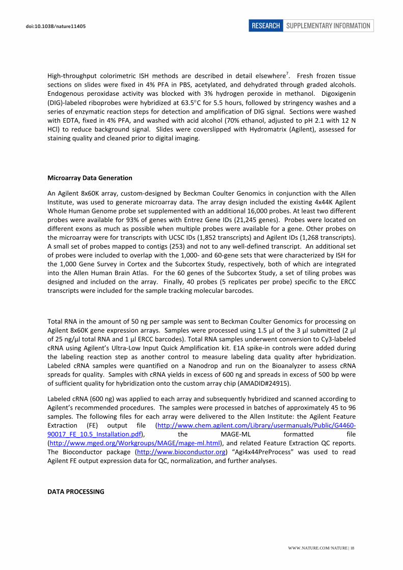
High‐throughput colorimetric ISH methods are described in detail elsewhere7. Fresh frozen tissue sections on slides were fixed in 4% PFA in PBS, acetylated, and dehydrated through graded alcohols. Endogenous peroxidase activity was blocked with 3% hydrogen peroxide in methanol. Digoxigenin (DIG)‐labeled riboprobes were hybridized at 63.5°C for 5.5 hours, followed by stringency washes and a series of enzymatic reaction steps for detection and amplification of DIG signal. Sections were washed with EDTA, fixed in 4% PFA, and washed with acid alcohol (70% ethanol, adjusted to pH 2.1 with 12 N HCl) to reduce background signal. Slides were coverslipped with Hydromatrix (Agilent), assessed for staining quality and cleaned prior to digital imaging.

Microarray Data Generation

An Agilent 8x60K array, custom‐designed by Beckman Coulter Genomics in conjunction with the Allen Institute, was used to generate microarray data. The array design included the existing 4x44K Agilent Whole Human Genome probe set supplemented with an additional 16,000 probes. At least two different probes were available for 93% of genes with Entrez Gene IDs (21,245 genes). Probes were located on different exons as much as possible when multiple probes were available for a gene. Other probes on the microarray were for transcripts with UCSC IDs (1,852 transcripts) and Agilent IDs (1,268 transcripts). A small set of probes mapped to contigs (253) and not to any well‐defined transcript. An additional set of probes were included to overlap with the 1,000‐ and 60‐gene sets that were characterized by ISH for the 1,000 Gene Survey in Cortex and the Subcortex Study, respectively, both of which are integrated into the Allen Human Brain Atlas. For the 60 genes of the Subcortex Study, a set of tiling probes was designed and included on the array. Finally, 40 probes (5 replicates per probe) specific to the ERCC transcripts were included for the sample tracking molecular barcodes.

Total RNA in the amount of 50 ng per sample was sent to Beckman Coulter Genomics for processing on Agilent 8x60K gene expression arrays. Samples were processed using 1.5 µl of the 3 µl submitted (2 µl of 25 ng/µl total RNA and 1 µl ERCC barcodes). Total RNA samples underwent conversion to Cy3‐labeled cRNA using Agilent’s Ultra‐Low Input Quick Amplification kit. E1A spike‐in controls were added during the labeling reaction step as another control to measure labeling data quality after hybridization. Labeled cRNA samples were quantified on a Nanodrop and run on the Bioanalyzer to assess cRNA spreads for quality. Samples with cRNA yields in excess of 600 ng and spreads in excess of 500 bp were of sufficient quality for hybridization onto the custom array chip (AMADID#24915).

Labeled cRNA (600 ng) was applied to each array and subsequently hybridized and scanned according to Agilent’s recommended procedures. The samples were processed in batches of approximately 45 to 96 samples. The following files for each array were delivered to the Allen Institute: the Agilent Feature Extraction (FE) output file (http://www.chem.agilent.com/Library/usermanuals/Public/G4460‐90017_FE_10.5_Installation.pdf), the MAGE‐ML formatted file (http://www.mged.org/Workgroups/MAGE/mage‐ml.html), and related Feature Extraction QC reports. The Bioconductor package (http://www.bioconductor.org) “Agi4x44PreProcess” was used to read Agilent FE output expression data for QC, normalization, and further analyses.

DATA PROCESSING



Microarray Data Processing

Initial Data Quality Control

The first steps in microarray data processing were assessing the overall data quality. Every sample went through basic QC steps, including recording and assessment of: 1) the 99% non‐control probe signal, 2) visual inspection of array thumbnails, 3) %CV of non‐control probes, 4) E1A control signal, 5) outlier detection (all metrics available in Agilent’s Feature Extraction (FE) output).

Default GE1 QC thresholds were used as initial quality control criteria of the microarray data (see Table 4). Any arrays with values outside of the threshold ranges were further evaluated. If an explanation for the values outside of threshold could not be determined the array was failed. Furthermore, we also visually assessed and recorded notes for the Spatial Distributions of All Outliers, the Spot Finding of the Four Corners of the Array and the Histogram of Signal Plots for each individual array. This was done to track both hybridization performance and RNA sample quality (Figures can be found on pages 65‐67 of Agilent Feature Extraction Software Reference Guide v10.5).

Table 4. Evaluation metrics for initial microarray data quality control.

Metric Name Value Upper Limit

Lower Limit Is Mandatory

AnyColorPrcntFeatNonUnif 0.01 1.0 NA FALSE

DetectionLimit 1.38 2.0 0.01 FALSE

absGE1E1aSlope 0.99 1.2 0.9 FALSE

gE1aMedCVProcSignal 4.30 8.0 NA FALSE

gNegCtrlAveBGSubSig ‐2.64 5.0 ‐10 FALSE

gNegCtrlAveNetSig 28.6 40.0 NA FALSE



gNegCtrlSDevBGSubSig 2.60 10.0 NA FALSE

gNonCntrlMedCVProcSignal 4.72 8.0 NA FALSE

gSpatialDetrendRMSFilter 3.44 15.0 NA FALSE

In addition, a heuristic detection rule was designed to identify outlier candidates for each batch (see Table 5). Samples identified as outliers were resubmitted for microarray data generation.

Table 5. Outlier detection based on Inter‐Array Connectivity (IAC).

Sample Capture Method When, IQD(IAC of batch) Sample is called an outlier, IF

IQD(IAC) ≥ 0.02 IAC(s) < 0.92 Macrodissection

IQD(IAC) < 0.02 IAC(s) < 0.92, s is in lowest 5% end

IQD(IAC) ≥ 0.02 IAC(s) < 0.80, s is in lowest 5% end LMD

IQD(IAC) < 0.02 Samples in lowest 5% end

IAC of a sample is the mean of correlation values between the sample and all other samples in the batch. Inter‐Quartile Distance (IQD) of IAC is used to identify the range of the distribution of IAC.

The ERCC transcripts were used to detect possible errors in sample handling related to mixing samples in wells or inadvertently loading an incorrect sample onto a particular array. Microarray data for ERCC specific probes were assessed using a heat map to track placement of samples. The quality control process included confirming that only the expected row and column spiked transcripts showed signal above background. Samples were failed if they did not contain exclusively the ERCC transcripts spiked into the RNA well. Figure 5 below shows an example heat map in which a sample event mimicking cross‐contamination was detected.



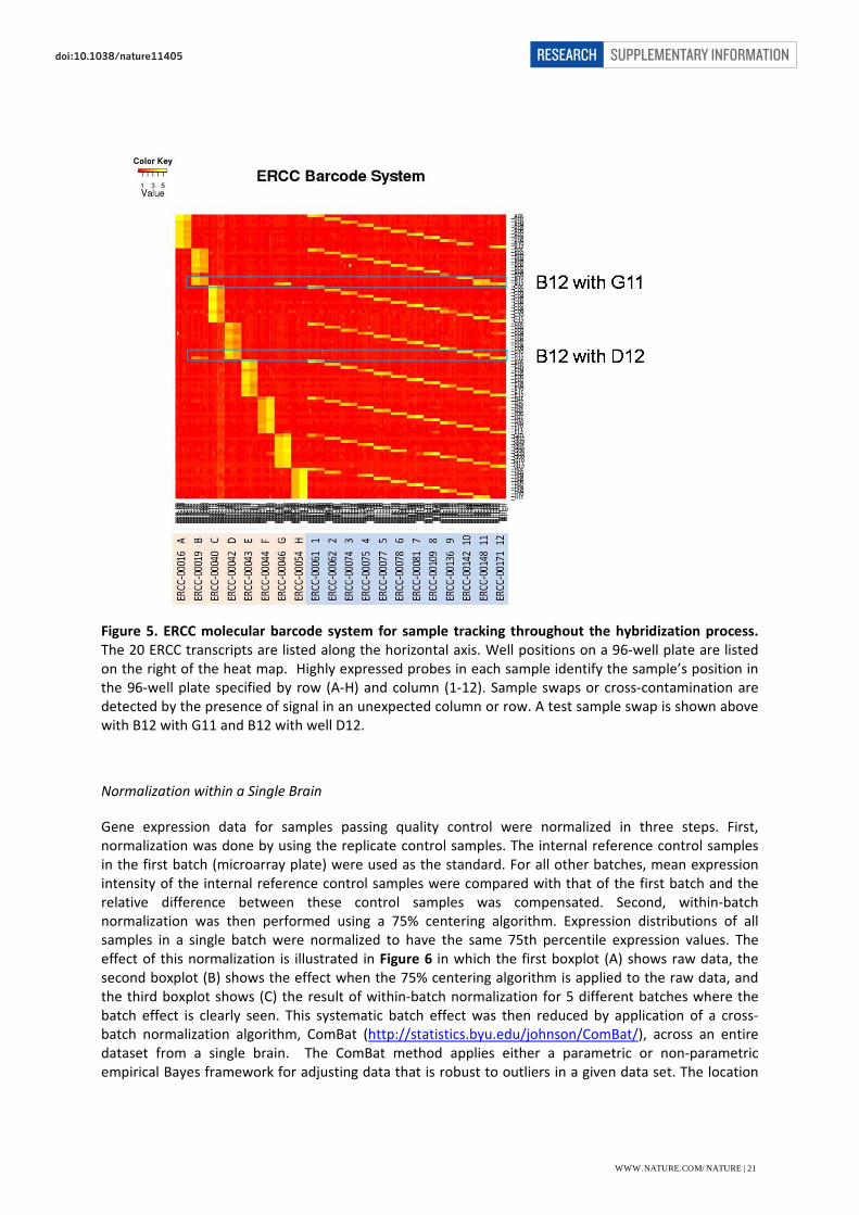
Figure 5. ERCC molecular barcode system for sample tracking throughout the hybridization process. The 20 ERCC transcripts are listed along the horizontal axis. Well positions on a 96‐well plate are listed on the right of the heat map. Highly expressed probes in each sample identify the sample’s position in the 96‐well plate specified by row (A‐H) and column (1‐12). Sample swaps or cross‐contamination are detected by the presence of signal in an unexpected column or row. A test sample swap is shown above with B12 with G11 and B12 with well D12.

Normalization within a Single Brain

Gene expression data for samples passing quality control were normalized in three steps. First, normalization was done by using the replicate control samples. The internal reference control samples in the first batch (microarray plate) were used as the standard. For all other batches, mean expression intensity of the internal reference control samples were compared with that of the first batch and the relative difference between these control samples was compensated. Second, within‐batch normalization was then performed using a 75% centering algorithm. Expression distributions of all samples in a single batch were normalized to have the same 75th percentile expression values. The effect of this normalization is illustrated in Figure 6 in which the first boxplot (A) shows raw data, the second boxplot (B) shows the effect when the 75% centering algorithm is applied to the raw data, and the third boxplot shows (C) the result of within‐batch normalization for 5 different batches where the batch effect is clearly seen. This systematic batch effect was then reduced by application of a cross‐batch normalization algorithm, ComBat (http://statistics.byu.edu/johnson/ComBat/), across an entire dataset from a single brain. The ComBat method applies either a parametric or non‐parametric empirical Bayes framework for adjusting data that is robust to outliers in a given data set. The location



(mean) and scale (variance) model parameters were specifically estimated by pooling information across genes in each batch to shrink the batch effect parameter estimated toward the overall mean of the batch effect estimates. After the ComBat algorithm was applied, the differences between batches disappear, as shown in Figure 6D. Raw expression values, within‐batch normalized expression values, and cross‐batch normalized expression values were all uploaded into the database for further data analyses and data visualization.

Figure 6. Effect of 75% centering normalization algorithm and cross‐batch normalization over 5 data batches. The first boxplot (A) shows the distribution of raw expression values for each sample prior to any normalization. The second boxplot (B) shows the application of the 75% centering algorithm to all samples. The third boxplot (C) displays the result of applying the 75% centering algorithm to each batch separately, e.g., within‐batch normalization. The fourth boxplot (D) shows cross‐batch normalization with the ComBat algorithm applied to the within‐batch normalized data from (C).

Normalization across Multiple Brains

To allow comparison of microarray data across 2 or more brains, a final cross‐brain normalization was performed by aligning the mean 75th percentile expression values of all internal reference control samples of each brain to that of the first brain.

A B C D



Digital Imaging and Processing of Histologically Stained Sections

Digital imaging of 6x8 large format slides was performed the Kodak/Creo flatbed iQsmart3 scanner at 215,000 dpi resolution (4.65 µm/pixel). Endpoint adjustments were done prior to scanning to compensate for variance in light intensity across each slide. Digital imaging of 2x3 slides was done using the ScanScope XT (Aperio Technologies, Vista, CA) with slide autoloader. Gain adjustments were made to lighten background for the darker silver stain. Final resolution of 2x3 images was 1 µm/pixel. All images were databased and preprocessed, then assessed for quality to ensure optimal focus and that no process artifacts were present on the slide images. Images that passed this initial QC were further assessed to ensure that the staining data were as expected. Once all QC criteria were met, images became available for annotation of anatomic structures as well as for anatomic visualization and mapping processes described below.

MR Image Postprocessing

All T1‐weighted volumes were anatomically segmented using the standardized recon‐all pipeline FreeSurfer image analysis suite, which is documented and freely available for download online (http://surfer.nmr.mgh.harvard.edu/). Technical details of these processes are described elsewhere (for examples, see 8‐10). In short, intensity inhomogeneity correction, tissue classification (grey/white matter and cerebrospinal fluid), skull stripping, cortical surface reconstruction, and cortical and subcortical segmentation of structures based on tissue class likelihood estimates, geometric features, and structure‐wise likelihood estimates were performed. The pipeline required an initial matching of the each T1‐weighted scan to MNI‐space. While the standard pipeline is capable of accomplishing this, in cases where the initial linear MRI‐to‐MNI space transformation estimation procedure failed, a manually initialized affine transformation was estimated through the placement of homologous landmark pairs in register, part of the MNI/MINC toolbox (http://www.bic.mni.mcgill.ca/ServicesSoftware/HomePage).

Anatomic Mapping and Visualization

To enable unified navigation and visualization, spatial correspondences between 2x3 images, 6x8 images and MR volumes were obtained via a series of assisted registration processes. Registration started with the construction of virtual slab images by creating mosaics from representative Nissl images from 2x3 blocks. Typically, the last image from a block Nissl series, where macrodissection sites were annotated, was chosen as the representative image. For each slab, a SVG (scalable vector graphics) file was created containing pointers to downsampled representative block images. Each block was visually placed (rotated and translated) into its correct orientation using Inkscape (http://www.inkscape.org; an open source SVG editor) creating a virtual slab image. The transform parameters for each block was parsed from the SVG file and saved for downstream use.

In the next step, each virtual slab image was placed in context of the T1 weighted MR volume. The removal of the cerebellum and brain stem from the cerebrum during tissue dissection caused significant deformation compared to the brain in its native conformation in the skull. Further deformation was introduced during the slabbing procedure where the type and severity of the distortion varied from slab to slab. The severity of the overall deformation necessitated an intensive landmark based registration process in order to establish spatial correspondences. For each slab, 50 to 100 corresponding landmark



points were manually placed on the virtual slab image and T1 MR volume using the facility provided by BioImage Suite (http://www.bioimagesuite.org). The landmark information was saved as text files for further processing. Initially, a “best‐fit” affine transform was estimated that coarsely oriented a slab within the 3D MR volume. A deformation field was then estimated from the remaining displacement using thinplate radial base function interpolation.

As needed other block images were registered to the “representative” block image. Similarly other slab‐based images (blockface, 6x8 images) were registered to the “virtual” slab image. These additional transforms combined with those described above allowed spatial correspondences to be established between 2x3 images, 6x8 images and MR volumes.

Results from the registration processes above allowed the construction of MR‐based navigation maps shown in 2D triplanar view. For each position in 3D MR space, a nearest slab and nearest block were pre‐computed allowing the use of the 3D MR volumes to navigate through different slabs and blocks. Inversely, information annotated in block images was projected back into MR space. For example, the “center” location of macrodissection and LMD dissection sites were mapped back into MR space and used as representative locations for visualization the spatial variation in gene expression for each probe.



QC AND SCIENTIFIC QUALITY ASSESSMENT

To ensure quality data, numerous QC checkpoints were incorporated throughout the entire microarray data production pipeline for the Allen Human Brain Atlas, as illustrated diagrammatically in Figure 7. Such QC checkpoints were used to qualify material to advance further down the pipeline and to measure, trend and improve all phases of laboratory operations.

The major QC processes and steps indicated in Figure 7 are summarized in Table 6. These range from tissue qualification and assessment through generation and final qualification of the data for inclusion in the online public resource.

Table 6. QC steps.

QC Step Description

Q1 Gross evaluation of the frozen, slabbed brain upon receipt after shipping. The tissue was evaluated for issues that include breakage, surface irregularities, and freezing and storage artifacts. Each slab is assigned a pass/fail score based on these variables.

Q2 Evaluation of full‐coronal tissue sections. Each section was checked for adhesion to the glass slide, tissue integrity, wrinkles, and drying artifacts.

Q3 Histology assessment. Each stained section was assigned a quality score (1‐failing to 5‐excellent) based on stain quality, tissue quality and observed artifacts.

Q4 Evaluation of tissue blocks created by subdivision of frozen slabs. Each resulting tissue block was evaluated for tissue quality and anatomic accuracy of subdivision.

Q5 (& Q15) Evaluation of tissue sections on 2x3 slides. Each section was checked for adhesion to the glass slide, tissue integrity, wrinkles, and drying artifacts.

Q6 (& Q13) Histology assessment. Each stained section was assigned a quality score (1‐failing to 5‐excellent) based on stain quality, tissue quality and observed artifacts.

Q7 (& Q14) Post‐dissection validation of tissue sampling. The accuracy and quality of each dissected sample was compared to annotated images of the region to ensure the correct anatomic areas were captured.

Q8 (& Q12) Post‐scanning assessment of 2x3 histology images. Each digital image was checked for orientation, focus, white balance, staining quality and tissue quality. Failed images were excluded from further processing.



Q9 (& Q11) RNA assessment. Quantity and quality of total RNA isolated from dissected tissue samples was evaluated.

Q10 Microarray expression assessment. All microarray data were analyzed to identify outliers and to verify that the correct samples were processed and associated with the correct brain region. For samples identified as outliers or incorrectly tracked, microarrays were rerun.

Q11 See Q9.

Q12 See Q8.

Q13 See Q6.

Q14 See Q7.

Q15 See Q5.

Q16 Assessment of blockface images. Each blockface image was evaluated for focus, image quality and orientation at the time of image acquisition, thereby allowing real‐time adjustments to ensure that each image passed QC.

Q17 MRI assessment. Each set of imaging data was evaluated for contrast, consistency of signal across the dataset and signal‐to‐noise ratio.

Q18 cRNA QC. Each cRNA product is evaluated for yield and product size.



Figure 7. Data production pipeline indicating key QC steps for the whole brain microarray survey of the Allen Human Brain Atlas. CRC is the Case Review Committee, a group of experts that evaluate the available donor and tissue information to qualify cases for data generation. µNP is the microneuropathology screen. LIMS is the Laboratory Information Management System in which all data are tracked and processed for presentation of data online.




Construction of Landscape Plot and Visualization

The open source software graphics package R (http://www.r‐project.org/) was extensively used for the plotting and visualization in Figure 2 of the main manuscript and Supplementary Figure 1. To transform expression values into the same scale across genes, the median expression value for a given gene was subtracted. Since most genes were represented by more than one probe, the best probe for each gene was identified by best correlation across 146 regions between the two brains. Expression plots for the neurotransmitter pathways were generated based on these expression values. After transformation

into linear expression values by a 2x transformation, expression values were truncated at 20. These R graphics methods are available on request.

For the PSD plot in Figure 2b of the main manuscript, PSD genes were ranked by regional fold expression difference and confirmation of the significance of the differential expression was performed post hoc. Briefly, each gene's expression values were averaged across regions of the same name in both hemispheres (if relevant), and the maximal and minimal‐expressing regions were identified. The averaged log2 expression values of the maximal and minimal‐expressing regions were subtracted to obtain the fold difference in expression. Significance of the expression difference was computed using the expression values from the original samples in the maximal and minimal‐expressing regions. ANOVA of expression was performed with respect to which brain the sample was from and the region the sample was from. The p value for the main effect of brain region was corrected by the Benjamini‐Hochberg false discovery rate procedure. In Supplemental Table 3 we report the maximum and minimum‐expressing regions and false discovery rate (Benjamini‐Hochberg) of the expression difference which was always less than 1% (median FDR is 4e‐10 for the 74 highest fold‐change PSD genes).

Data Processing for Weighted Gene Coexpression Analyses

Unprocessed expression microarray data was collected and normalized as described in the main text. Then, the following preprocessing steps were applied: 1) omit the 11,673 probes that lack a Entrez Gene Id; 2) transform the expression data from log space to normal space; 3) remove outlier samples with exceptionally low inter‐array correlation (7 out of 918 samples were removed); 4) remove the 6,041 remaining probes that were present in <1% of the samples (as called by the Agilent software); 5) select the "best" probe for each gene using the function collapseRows in the WGCNA library11. Specifically, only the probe with the maximum connectivity (summed adjacency) was retained if there were at least three probes for a gene, otherwise the probe with the maximum variance was retained. After preprocessing, there were a total of 21,337 genes measured across 911 samples in Brain 1 that were used for WGCNA. Genes in Brain 2 were assigned using the same probes as in Brain 1 for between‐brain comparisons; thus, no data preprocessing from Brain 2 was required.

Network Formation and Module Characterization



For whole brain (all 911 samples) we created a network from normalized expression data by following the standard procedure of WGCNA12,13. Briefly, for each network we calculated pair‐wise Pearson correlations between each gene pair, and then transformed this matrix into a signed adjacency matrix using a power function. The components of this matrix (connection strengths) were then used to calculate "topological overlap" (TO), a robust and biologically meaningful measurement of gene similarity, which quantitatively assesses the similarity of two genes' coexpression networks12,14. In other words, a pair of genes whose "neighbors" are highly coexpressed will have high TO. Genes were hierarchically clustered using the 1‐TO as the distance measure, and initial module assignments were determined by using a dynamic tree‐cutting algorithm15. Final module assignments were then found by adjusting module characterizations based on general biological and statistical criteria (see below).

Modules in each network were characterized using several strategies. First, modules were annotated based on gene ontology enrichment using Enrichment Analysis Systematic Explorer16. Second, modules were further annotated by measuring their overlap with previous brain‐related lists using the function userListEnrichment in the WGCNA library and setting useBrainLists=TRUE11. These lists include modules from previous WGCNA studies of human and mouse brain, and experimentally‐derived marker genes for cell‐types, and region‐enriched and disease‐specific genes from previous microarray studies, and others (see the help file of this function for more details and references). Third, modules were characterized based on the expression of the module eigengene (ME), or the first principle component of the module. Specifically, bar plots showing the expression of MEs across brain subregions were created in order to assess the brain region specificity of each module. Finally, the Pearson correlation between each gene and each ME—referred to as a gene's module membership (kME)

17,18—was calculated. Representative ("hub") genes with high kME for some modules are presented in Figure 3c in main manuscript, while all kME values are reported in Supplementary Table 4.

Comparative Analyses Accompanying WGCNA

Several comparative analyses were performed using data from the network analyses, which generally fall into two categories: comparisons between brain regions (within Brain 1) and comparisons across brains. To visualize the region‐enrichment of each gene within each region in the whole brain network, t values of samples in a given region were compared with all samples not in that region using a Student's t‐test, and were then plotted with red representing higher expression and green representing lower expression in that region relative to other regions. The 25 top‐level regions were then sorted manually to highlight regions with similar highly expressed genes (with the exception of subthalamus and white matter which had too few samples to perform this comparison). For each region in the whole brain network, we then assessed the preservation of each module, basically showing for which regions the overall coexpression patterns of each module are also present. Module preservation was calculated as described previously19. In short, several density measures assessing how tightly connected genes are in a module and several connectivity measures quantifying whether the internal structure (i.e., hub genes) is preserved are calculated, after which the resulting statistical significances are summarized by a single number. Values of this Z summary statistic that are ~10 or greater suggest significant module preservation between data sets.

Expression levels of select MEs were also shown summarized at the level of subregions. In this case, bars represent the average expression of each sample within a given subregion, with error bars showing standard error. The significance of overall regionality was calculated using a Kruskall‐Wallis one‐way ANOVA (all p‐values are highly significant, but are not shown). Bar graphs are displayed following an



anatomically relevant order, which can be approximated as follows: first, neocortical and then subcortical structures are ordered approximately rostral to caudal, with exceptions made for regions that are more anatomically similar and due to the fact that the brain has three dimensions; second, within each structure samples have rostral to caudal ordering (based on slab number); and finally, samples are ordered left‐to‐right hemisphere within each slab.

In addition to the between‐region comparisons, two comparisons between data sets were done in the whole brain network. First, module preservation was performed between Brain 1 and Brain 2, and between Brain 1 and the human network from20, as described above. Second, correlation of average gene expression between Brain 1 and Brain 2 across the 170 subregions with samples in both brains was calculated. For each gene, the average expression levels of these 170 subregions were calculated in both brains (as in Figure 3 in the main manuscript), with the resulting values in Brains 1 and 2 matched, correlated, and visualized.

Finally, a consensus network across all three brains was created by finding the TO matrix individually for each brain (as described above) and then using the component‐wise minimum value as input into downstream analyses21. Module assignments from Brain 1 (Figure 3b in the main manuscript) were then imposed on this consensus network, and MEs were calculated in Brains 2 and 3 using these modules.

Construction of Differential Correlograms and Clustering

Differential fold change relationships were recorded for all genes between all pairs of 146 structures for which at least two samples were available in both brains. Fold changes of at least 1.5 log2 were recorded and corrected for multiple hypothesis testing using Benjamini‐Hochberg (p < 0.01) method in the statistical package R (http://www.r‐project.org/). Both the number of differential relationships and the average magnitude of the highest fold changes were recorded. Through scaling with a jet color heat map and RColorBrewer package this enabled the visualizations in Figure 4a of the main manuscript and Supplementary Figures 2 and 3. Structural delineations were annotated by anatomists. Heatmap clustering was performed using the method heatmap.2 in R with appropriate color palate choice and ordering by anatomy fixed.




Computation of Regionally Enriched Marker Genes

Genes that are regionally over‐represented in expression were identified by computing the ratio of gene expression in a local structure to expression in the complementary set of structures in a larger macrostructure not containing the given structure. Genes were recorded as markers if they exhibited a 2‐fold enrichment in a particular subregion compared to the combined set of complementary regions. For example, a marker gene for CA2 in the hippocampus has 2‐fold enrichment in CA2 compared to CA1, CA3, CA4, subiculum, and dentate gyrus combined. These relationships are fully determined by the structural ontology presented in Supplementary Table 2.

Cortical Analysis and Reconstruction

Cortical samples were pooled to 56 cortical subregions and a mean gene expression score for each gene in each subregion was computed. These data were Z‐score normalized for consistent scaling across genes and hierarchically clustered in the R statistical package. Principal component analysis and multidimensional scaling were performed using the R package as well. To obtain the representation in Figure 6e of the main manuscript, multidimensional scaling (MDS) was used. Given only a set of distances defined between points in a higher dimensional space (in this case gene expression vectors of cortical samples), this method seeks to find a lower dimensional embedding of the original unknown coordinate points (usually dimension 2 or 3) that approximates the distance relationships in a least squared sense. Closely related to standard PCA, the coordinate vectors along these projected dimensions can be shown to be equivalent to coordinates along the principal component vectors in a standard PCA representation22. For each gene from the 1000 most differential gene set an expression vector across the 56 samples is formed. (The method works equivalently using any gene set.) Correlation between these samples allows a genetic distance between samples 1 2,s s to be defined as

21 2 1 2( , ) 1 ( , ) .d s s s sρ= − This distance matrix is input to the MDS algorithm producing the coordinate

embedding to the 2D representation shown in Figure 6e in the main manuscript.

Using the mapping of the samples into the MNI space representation one can compute the correlation of gene expression as a function of physical distance in the cortex. We first inflate the cortex to a spherical representation using FreeSurfer8 (http://surfer.nmr.mgh.harvard.edu/) so as to compare distances more accurately along a representation of the cortical plate. Correlation of gene expression vectors of length 1000 at each physical distance in Montreal Neurological Institute (MNI) space were computed and lowest fit with f = 1/4 in the statistical package R. Error bars are presented as the standard error of the mean.

Least Squares Fitting in 3D with Respect to Translation, Rotation, and Scaling

The representation of Figure 6e of the main manuscript using MDS provides a representation for relatively relocating samples on the cortical plate using genetic distance alone. Using appropriate centering, rotation, and scaling operations we can compute how close this representation is to the



actual sample coordinates as determined by the native MNI representation. The mathematics of this approach is described below.

We are given two collections of vectors iv and ib in 3D space. We can assume without loss of

generality that both collections are mean‐centered. We want to calculate the optimal orthogonal transformation R and scale factor s that minimizes the squared distance

∑ −=i

ii bsRvRsF 2),( .

Quaternions

The general transformation sRT = where R is an orthogonal transformation and s is a positive scalar can be written as

⎥⎥⎥

⎦

⎤

⎢⎢⎢

⎣

⎡

+−−+−−−+−++−−−+

=2222

2222

2222

222222222222

dcbaabcdacbdabcddcbabcadacbdadbcdcba

T

with 2222 dcbas +++= .

For ease in writing some equations, it is convenient to let au =1 , bu =2 , cu =3 , du =4 . In this

notation

∑=

=4

1,kjjkkj KuuT

where each jkK is defined as a 33× matrix entry in this 44× block matrix:

⎟⎟⎟⎟⎟

⎠

⎞

⎜⎜⎜⎜⎜

⎝

⎛

+−−++−+−+−+−++−−−−−−

=

TTTTTTTTT

TTTTTTTTT

TTTTTTTTT

TTTTTT

eeeeeeeeeeeeeeeeeeeeeeeeeeeeeeeeeeeeeeeeeeeeeeeeeeeeeeeeeeeeeeeeeeI

K

332211322331132112

322333221112211331

311312213322113223

211213313223

.



To simplify the equations, we introduce a scaling to the data. We let ∑=i

ibB 2 and

∑=i

ivV 2. Then if we let VtBs /= we can write

∑∑ −=−=i

iii

ii BbVtRvBbsRvRsF 222 //),( .

In other words, the minimum squared error is always some factor of the sum of the squares of the coordinates of the data. To find the minimum error factor, it suffices to assume that both B and V are scaled to equal 1. We can easily solve this minimization problem:

minimize 2( , , , ) .i i

iG a b c d Tv b= −∑

Note that ),(21),(2),( 2222iiiiiiiiiiii bTvsbTvbTvbTvbTvbTv −+=−+=−−=− . Thus we

have

⎥⎥⎥

⎦

⎤

⎢⎢⎢

⎣

⎡

−−

−=+++=

∂∂

=abcbad

cdadKcKbKaK

aTTa 22222 14131211

⎥⎥⎥

⎦

⎤

⎢⎢⎢

⎣

⎡

−−−=+++=

∂∂

=badabc

dcbdKcKbKaK

bTTb 22222 24232221

⎥⎥⎥

⎦

⎤

⎢⎢⎢

⎣

⎡

−−

−=+++=

∂∂

=cda

dcbabc

dKcKbKaKcTTc 22222 34333231

⎥⎥⎥

⎦

⎤

⎢⎢⎢

⎣

⎡−−−

=+++=∂∂

=dcbcdabad

dKcKbKaKdTTd 22222 44434241 .



With these equalities we can calculate the equations that determine the critical solutions:

asbvTaG

ii

ia 4),(20 +−=∂∂

= ∑

bsbvTbG

ii

ib 4),(20 +−=∂∂

= ∑

csbvTcG

ii

ic 4),(20 +−=∂∂

= ∑

dsbvTdG

ii

id 4),(20 +−=∂∂

= ∑

2222 dcbas +++= .

Thus we have to solve

⎟⎟⎟⎟⎟

⎠

⎞

⎜⎜⎜⎜⎜

⎝

⎛

=

⎟⎟⎟⎟⎟

⎠

⎞

⎜⎜⎜⎜⎜

⎝

⎛

dcba

s

dcba

M

where the kj, entry of the matrix M is given by ∑i

ijkTi vKb . This equation has the form

xxMx 2||||= .We can solve this equation by examining the eigenvalue equation yMy λ= . Let y be a

unit norm eigenvector with eigenvalue λ . Let λyx = . Then λ== 2|||| xs and

xxxMx 2||||== λ . In particular, for each solution x



24

1,

),( sMxxvuKubbTv T

i kjikjkj

Ti

iii === ∑ ∑∑

=

.

Finally, we see that at the critical points

222 11),( λ−=−=−= ∑ sbsRvRsFi

ii

so the optimal solution occurs at the eigenvalue that is largest in magnitude.

What fraction of the data is explained by the model?

We address this first as a more general problem. Suppose we are given a unit vector u and an approximation vector v , which comes from a model. What fraction of u is explained by v ? One measure of this fraction is the projection of u onto v . In the case where the error vector vu − is orthogonal to the model vector v , this is very simply solved using the leg rule for a right triangle: the square of one side is equal to the product of the hypotenuse and the corresponding leg formed by the altitude. In the present case, the hypotenuse has length 1 so this says that the length of the projection is the square of the length of the model vector. Thus in this case the fraction of the data explained by the model is the square of the length of the model vector.

To apply this to our model, note that we have scaled the problem so that the length of the data vector is

1, the length of our model vector is λ=s and the length of the error vector is 21 λ− . Thus the error vector is orthogonal to the model vector and the fraction of the data explained by the model is the

square of the length of the model vector, namely the square of the eigenvalue 2λ .



References

1 Atz, M. et al. Methodological considerations for gene expression profiling of human brain. J Neurosci Methods 163, 295‐309 (2007).

2 Durrenberger, P. F. et al. Effects of antemortem and postmortem variables on human brain mRNA quality: a BrainNet Europe study. J Neuropathol Exp Neurol 69, 70‐81 (2010).

3 Schroeder, A. et al. The RIN: an RNA integrity number for assigning integrity values to RNA measurements. BMC Mol Biol 7, 3 (2006).

4 Proposed methods for testing and selecting the ERCC external RNA controls. BMC Genomics 6, 150 (2005).

5 Culling, C. F. A., Allison, R. T. & Barr, W. T. Cellular Pathology Technique. Fourth edn, 160‐161 (Butterworths, 1985).

6 Garvey, W., Fathi, A., Bigelow, F., Jiminez, C. & Carpenter, B. A reliable silver impregnation technique for the nervous system. J Histotechnology 10, 245‐247 (1987).

7 Lein, E. S. et al. Genome‐wide atlas of gene expression in the adult mouse brain. Nature 445, 168‐176 (2007).

8 Dale, A. M., Fischl, B. & Sereno, M. I. Cortical surface‐based analysis. I. Segmentation and surface reconstruction. NeuroImage 9, 179‐194 (1999).

9 Fischl, B. et al. Whole brain segmentation: automated labeling of neuroanatomical structures in the human brain. Neuron 33, 341‐355 (2002).

10 Segonne, F. et al. A hybrid approach to the skull stripping problem in MRI. NeuroImage 22, 1060‐1075 (2004).

11 Miller, J. A. et al. Strategies for aggregating gene expression data: The collapseRows R function. BMC Bioinformatics. 12, 322. (2011).

12 Zhang, B. & Horvath, S. A general framework for weighted gene co‐expression network analysis. Stat Appl Genet Mol Biol 4, Article17 (2005).

13 Horvath, S. et al. Analysis of oncogenic signaling networks in glioblastoma identifies ASPM as a molecular target. Proc Natl Acad Sci U S A 14, 17402‐17407 (2006).

14 Ravasz, E., Somera, A. L., Mongru, D. A., Oltvai, Z. N. & Barabasi, A. L. Hierarchical Organization of Modularity in Metabolic Networks. Science 297, 1551‐1555 (2002).

15 Langfelder, P., Zhang, B. & Horvath, S. Defining clusters from a hierarchical cluster tree: the Dynamic Tree Cut package for R. Bioinformatics. 24, 719‐720. Epub 2007 Nov 2016. (2008).

16 Hosack, D. A., Dennis, G., Sherman, B. T., Lane, H. C. & Lempicki, R. A. Identifying biological themes within lists of genes with EASE. Genome Biology 4 (2003).

17 Horvath, S. & Dong, J. Geometric interpretation of gene coexpression network analysis. PLoS Comput Biol 4, e1000117 (2008).

18 Oldham, M. C. et al. Functional organization of the transcriptome in human brain. Nat Neurosci 11, 1271‐1282 (2008).

19 Langfelder, P., Luo, R., Oldham, M. & Horvath, S. Is my network module preserved and reproducible? PLoS computational biology 7, e1001057 (2011).

20 Miller, J., Horvath, S. & Geschwind, D. Divergence of human and mouse brain transcriptome highlights Alzheimer disease pathways. Proceedings of the National Academy of Sciences of the United States of America 107, 12698‐12703 (2010).

21 Langfelder, P. & Horvath, S. WGCNA: an R package for weighted correlation network analysis. BMC Bioinformatics 9, 559, doi:1471‐2105‐9‐559 [pii]10.1186/1471‐2105‐9‐559 [doi] (2008).

22 Cox, T. F. & Cox, M. A. A. Multidimensional scaling. (Chapman and Hall, 2001).



supplementary information - media.nature.com · cut using a disposable stainless steel dissection...

Documents