supervisor: professor rui manuel menezes carneiro de ... · given according to a buckling mode) may...

ASPECTS ON NONLINEAR GEOMETRIC AND MATERIAL ANALYSIS OF THREE-DIMENSIONAL FRAMED STRUCTURES

ALBANO ANTÓNIO DE ABREU E PRESA DE CASTRO E SOUSA

Dissertation submitted for partial satisfaction of the requirements for the degree of

MASTER IN CIVIL ENGINEERING — SPECIALIZATION IN STRUCTURAL ENGINEERING

Supervisor: Professor Rui Manuel Menezes Carneiro de Barros, PhD

Co-Supervisor: Structural Engineer Miguel Pereira

JULHO DE 2009

MASTERS IN CIVIL ENGINEERING 2008/2009

DEPARTMENT OF CIVIL ENGINEERING

Tel. +351-22-508 1901

Fax +351-22-508 1446

� [email protected]

Edited by

FACULTY OF ENGINEERING OF THE UNIVERSITY OF PORTO

Rua Dr. Roberto Frias

4200-465 PORTO

Portugal

Tel. +351-22-508 1400

Fax +351-22-508 1440

� [email protected]

� http://www.fe.up.pt

Partial reproductions of this document are allowed on the condition that the Author is mentioned and that reference is made to Masters in Civil Engineering – 2008/2009 – Department of Civil Engineering, Faculty of Engineering of the University of Porto, Porto, Portugal, 2009.

The opinions and information included in this document represent solely the point of view of the respective Author, while the Editor cannot accept any legal responsibility or other with respect to errors or omissions that may exist.

This document was produced from an electronic version supplied by the respective Author.

Aspects On Nonlinear Geometric and Material Analysis of Three-Dimensional Framed Structures

No snowflake in an avalanche ever feels responsible.

Voltaire


i

ACKNOWLEDGEMENTS

To Professor Rui Carneiro de Barros and Structural Engineer Miguel Pereira for their overwhelming

enthusiasm, availability and patience to discuss the several critical aspects involved in the

development of this thesis.

To the engineering consulting firm AFAConsult and its entire staff a special thanks is due both for

welcoming me to their working space and for sharing their body of knowledge, along with making

available critical software in the development of this thesis – Fagus, Pyrus and Robot.

To Labest and its scientific coordinator, Professor Joaquim Figueiras, for making available the

computer program Diana.

To all the Professors that have assisted me in this thesis either by sharing their time, expertise or

critical bibliographical references: Professor José Miguel Castro, Professor Mário Pimentel, Professor

Rui Faria, Professor Manuel Braz César, Professor Xavier Romão, and Professor Raimundo Delgado.

To all my colleagues for their input and feedback on this thesis namely Ricardo Teixeira Pinto, Hélder

Francisco Xavier, Bruno Duarte, Bruno Quintas Vieira, Pedro Julião Tavares, José Pedro Cabral,

Daniel Amaral, Edgar Brito, Vítor Resende and Valdir Pereira.

To my family, my father, my mother and my brother, for all their help and sacrifice, I convey my most

humble and heartfelt gratitude.


ii

Aspects On Nonlinear Geometric and Material Analysis of Framed Structures

iii

ABSTRACT

The design of three-dimensional framed structures, especially tall framed structures, is an analysis that

must take into account both geometric and material nonlinearities in an ultimate limit state. For

material nonlinearity, involving two of the most common materials (concrete and steel), this involves

addressing both short term and long term effects; the former having to do with cracking and nonlinear

stress-strain relations, and the latter with creep, shrinkage and relaxation. With respect to geometric

nonlinearities, these effects are well established for linear elastic materials.

This thesis will address several aspects of current state of the art methodologies that are used to study

both geometric and material nonlinearities in conjunction. It will also discuss the basic simplified

procedures that current codes practice allow for the design of frames as a way to bypass a more

rigorous and advanced analysis, as it is also a more expensive, complex and time consuming one.

On the subject of geometric nonlinearity an in-depth analysis on the issue of effective lengths is made,

as well as a comparison between several codes of practice.

Stiffness reductions factors, recommend by various design codes, are put to test through an advanced

nonlinear geometric and material analysis of: 140 reinforced concrete beams; 252 reinforced concrete

columns; and 252 concrete encased composite steel-concrete columns, including effects of, not often

modeled, different end restraints on the structural members.

As for the analysis of three-dimensional framed structures, a methodology is proposed from an

extension of CEB-FIP’s Model Code 90 procedures, so that a practical second-order linear elastic

analysis using the effective stiffness of a cross-section, made any material, can be done. Since the

analysis must involve the effects of geometrical imperfections, and since these deformations (usually

given according to a buckling mode) may not have the same direction as the deformed shape that

arises from external loading, a way assuring the compatibility of these displacements is addressed. The

proposed method is numerically tested and its principal limitations are outlined.

KEYWORDS: nonlinear, geometric, material, effective length, stiffness reduction, spatial frames


iv


v

RESUMO

O dimensionamento de estruturas porticadas tridimensionais, especialmente estruturas altas, é uma análise ter em conta não linearidades geométricas e materiais em estado limite último. Em relação à não linearidade material que envolve os dois tipos de materiais mais correntes (betão e aço), este tipo de análise terá que abordar efeitos tanto a curto como a longo prazo: fendilhação e relações tensão-extensão não lineares, a curto prazo; e fluência, retracção e relaxação, a longo prazo. Os efeitos da não linearidade geométrica segundo a teoria da elasticidade estão já bastante estabelecidos na literatura.

Esta tese procurará abordar vários aspectos do actual estado de arte no que concerne às várias metodologias usadas para tratar em conjuntos não linearidades geométricas e materiais. Procurará, igualmente, discutir os vários processos simplificados que alguns regulamentos prevêem como maneira de ultrapassar uma análise mais rigorosa e avançada, já que esta é, em geral, de alguma complexidade, onerosa e morosa.

No que diz respeito à não linearidade geométrica, é efectuada uma análise aprofundada em relação ao uso de comprimentos de encurvadura, bem como uma comparação entre as diferentes abordagens a esta metodologia são feitas por diversos regulamentos.

Reduções de rigidez recomendadas por alguns regulamentos são testadas através de uma análise não linear geométrica e material avançada a: 140 vigas de betão armado; 252 colunas de betão armada; e 252 colunas mistas de betão-aço, isto incluindo efeitos, não modelados frequentemente, de diferentes restrições nas extremidades dos elementos.

Já em relação à analise de estruturas porticadas tridimensionais, uma metodologia é proposta, através da extensão de um procedimento recomendado pelo Model Code 90 da CEB-FIP, a fim de efectuar uma análise linear elástica de segunda ordem prática, usando uma rigidez efectiva de uma secção constituída por qualquer tipo de material. Como este tipo de análise terá de ter em conta os efeitos de imperfeições geométricas e, como estas deformações (geralmente assumidas segundo um modo de encurvadura) são podem não ter a mesma direcção das provocadas pelo carregamento exterior, uma maneira de abordar a compatibilidade destes deslocamentos é discutida. A metodologia proposta é modelada numericamente e as suas principais limitações delineadas.

PALAVRAS -CHAVE: não linearidade geométrica, não linearidade material, comprimento de encurvadura, rigidez nominal, pórticos tridimensionais


vi


vii

GENERAL INDEX

ACKNOWLEDGEMENTS ............................................................................................................................ i

ABSTRACT .............................................................................................................................. iii

RESUMO ................................................................................................................................................... v

1. INTRODUCTION ............................................................................................................... 1

1.1. BACKGROUND TO THE THESIS ....................................................................................................... 1

1.2. OBJECTIVES ..................................................................................................................................... 1

1.3. OUTLINE OF THE CHAPTERS .......................................................................................................... 2

2. STATE OF THE ART .................................................................................................... 5

2.1. GEOMETRIC NONLINEARITY ............................................................................................................ 5

2.2. MATERIAL NONLINEARITY ............................................................................................................... 8

2.3. GEOMETRIC AND MATERIAL NONLINEARITY ................................................................................ 11

2.4. CONCLUSIONS................................................................................................................................ 11

3. CODES OF PRACTICE ............................................................................................ 13

3.1. EFFECTIVE LENGTH ....................................................................................................................... 13

3.1.1. THEORETICAL BACKGROUND ........................................................................................................... 13

3.1.2. EUROPEAN CODES OF PRACTICE – EUROCODES 2 AND3 .................................................................. 14

3.1.3. AMERICAN CODES OF PRACTICE – AISC AND ACI ............................................................................ 19

3.1.4. COMPARISON BETWEEN CODES OF PRACTICE ................................................................................. 28

3.2. STIFFNESS REDUCTIONS FACTORS .............................................................................................. 35

3.2.1. EUROCODE 2 .................................................................................................................................. 35

3.2.2. EUROCODE 4 .................................................................................................................................. 40

3.2.3. ACI ................................................................................................................................................ 41

3.2.4. BRIEF COMMENTARY ...................................................................................................................... 42

3.3. AMPLIFICATIONS DUE TO SECOND-ORDER EFFECTS ................................................................ 42

3.3.1. EUROCODE 2 .................................................................................................................................. 42

3.3.2. EUROCODE 3 .................................................................................................................................. 45

3.3.3. EUROCODE 4 .................................................................................................................................. 45

3.3.4. ACI ................................................................................................................................................ 46


viii

3.3.5. AISC ............................................................................................................................................ 47

3.3.6. MODEL CODE 90 ........................................................................................................................... 49

3.3.7. BRIEF COMMENTARY ...................................................................................................................... 50

3.4. CONCLUSIONS ............................................................................................................................... 51

4. GUIDELINES FOR PRACTICE ........................................................................ 53

4.1. EFFECTIVE LENGTH ...................................................................................................................... 53

4.2. STIFFNESS REDUCTION FACTORS FOR REINFORCED CONCRETE AND COMPOSITE

ELEMENTS ..................................................................................................................................... 56

4.2.1. REINFORCED CONCRETE STRUCTURAL ELEMENTS WITH NEGLIGIBLE AXIAL LOAD – ADJACENT

ELEMENTS ..................................................................................................................................... 56

4.2.2. COMPRESSED STRUCTURAL ELEMENTS .......................................................................................... 65

4.3. POTENTIAL FOR THE USE OF VISCO-ELASTIC MODELS IN NONLINEAR MATERIAL AND

GEOMETRIC ANALYSIS ................................................................................................................ 73

4.3.1. THEORETICAL BACKGROUND .......................................................................................................... 73

4.3.2. WORKED EXAMPLE AND VERIFICATION ........................................................................................... 77

4.4. CONCLUSIONS ............................................................................................................................... 82

5. 3D APPROACH FOR THE ASSESSMENT OF

SECOND-ORDER EFFECTS – AN EXTENSION

OF MC90 SIMPLIFIED METHOD .................................................................... 83

5.1. INTRODUCTION .............................................................................................................................. 83

5.2. EXAMPLES ..................................................................................................................................... 88

5.2.1. STRUCTURE 1 ................................................................................................................................ 89

5.2.2. STRUCTURE 2 ................................................................................................................................ 92

5.2.3. STRUCTURE 3 ................................................................................................................................ 94

5.2. CONCLUSIONS ............................................................................................................................... 97

6. FINAL REMARKS ......................................................................................................... 99

6.1. CONCLUSIONS ............................................................................................................................... 99

6.2. RECOMMENDED FUTURE DEVELOPMENTS ................................................................................ 100


ix

REFERENCES ............................................................................................................................. 103

ANNEXES ...................................................................................................................................... 105


x


xi

FIGURE INDEX

Figure 2.1 – Second-Order Effects In Building Frames – From [7] .......................................................... 5

Figure 2.2 – Comparison Between The Variation Of Determinants Of a) Flexibility Matrix and b) Stiffness Matrix .................................................................................................................. 7

Figure 2.3 – Model of Irregular Prestressed Concrete Cross-Section: a) Arbitrary Arrangements and Interior Openings; b) Contribution of Concrete Under Compression or Tension (Trapezoid i) – As Presented in [14]....................................................................................................... 9

Figure 2.4 – Finite Elements Models: a) One Dimensional; b)Two Dimensional; c) Three-Dimensional – Adapted From [16], [17] and [18], respectively. .............................................................. 10

Figure 3.1 – Infinitesimal Segment of a Statically Undetermined Column [8] ........................................ 13

Figure 3.2 – Loading of a Pinned – Fixed Column ................................................................................. 15

Figure 3.3 – Loading of a Pinned – Partially Fixed Column ................................................................... 17

Figure 3.4 – AISC Alignment Charts for Nonsway (a)) and for Sway (b)).............................................. 21

Figure 3.5 – Beam Pinned At Both Ends With Applied End Moments ................................................... 22

Figure 3.6 – Buckling modes for a one-storey frame - Nonsway (a)) and for Sway (b))........................ 23

Figure 3.7 – Multistory Frame Buckling Nonsway – Adapted from [23] ................................................. 24

Figure 3.8 – Multistory Frame Buckling Sway – Adapted from [23] ....................................................... 27

Figure 3.9 – Comparison of K-Factors given by EC2 and EC3 in NonSway ......................................... 30

Figure 3.10 – Comparison of K-Factors given by EC2 and EC3 in Sway .............................................. 30

Figure 3.11 – Comparison Between Codes of Practice for Nonsway .................................................... 33

Figure 3.12 – Comparison Between Codes of Practice for Sway - { }0.3;0.2;3.1∈fK .................... 33

Figure 3.13 – Comparison Between Codes of Practice for Sway - { }0.15;0.10;0.8;0.7∈fK ......... 34

Figure 3.14 – Simple Way to Accounting for Creep Effects – From [21] ............................................... 38

Figure 3.15 – Fully Cracked Elastic Cross-Section ................................................................................ 38

Figure 3.16 – Stiffness Reductions Factors For a Rectangular Cross-Section Beam in Short Term

Loading .............................................................................................................................. 40

Figure 3.17 – Representation Of The Simplified Method For Assessing The Maximum Displacement Due To Second-Order Effects – From [6] .......................................................................... 49

Figure 4.1 – Worked Example – Load Cases i) and ii); Nonsway a) and Sway b) ................................ 53

Figure 4.2 – Spacial Arrangement Of a Tested Beam [mm] – According to [27] ................................... 56

Figure 4.3 – Comparison Between Experimental and Numerical Modelling .......................................... 57

Figure 4.4 – Simply Supported Beam Under Uniform Transverse Loading ........................................... 58

Figure 4.5 – Different Types Of Constraints Analyzed For a Beam Under Uniform Transverse Loading59


xii

Figure 4.6 – Deformation Of A Beam For A CO3 Type Of Constraints ................................................. 60

Figure 4.7 – Stiffness Reduction Factors for Constraints CO1 ............................................................. 61



Figure 4.10 – Stiffness Reduction Factors for Constraints CO4 ........................................................... 63

Figure 4.11 – Comparison Between Averages And Code Requirements ............................................. 64

Figure 4.12 – Bending of a Beam-Column by End Moments ................................................................ 65

Figure 4.13 – Schematic Representation of the Modeled Columns ...................................................... 66

Figure 4.14 – Span Of Tested Eccentricities On An Interaction Diagram – Diagram from [32] ............ 67

Figure 4.15 – Stiffness Reduction Factors For 2,0=ϖ and 3=l ..................................................... 68



Figure 4.18 – Stiffness Reduction Factors For 2,0=ϖ ...................................................................... 70

Figure 4.19 – Composite Cross-Sections Analyzed – a) Section 1; b) Section 2; c) Section 3 ............ 71

Figure 4.20 – Stiffness Reduction Factors For Section 1 ...................................................................... 71



Figure 4.23 – Kelvin Model .................................................................................................................... 75

Figure 4.24 – Kelvin Chain Model ......................................................................................................... 76

Figure 4.25 – Multidirectional fixed cracking model [36] ....................................................................... 77

Figure 4.26 – Hordijk Softening Curve – Taken from [36] ..................................................................... 78

Figure 4.27 – Details and Testing Arrangements For The Columns [mm] – Taken from [17] .............. 78

Figure 4.28 – Results for Column C1 .................................................................................................... 79





Figure 5.1 – a) Deformed Structure and Its Approximation; b) Spatial Consideration of The Approximation ................................................................................................................. 83

Figure 5.2 – Projection of the First and Second Order Displacements of the Column in Plane XY ...... 85

Figure 5.3 – Projection of the First and Second Order Displacements of a Cantilever Column in Plane XY in a Simplified Loading ................................................................................................ 85

Figure 5.4 – Flow Chart Of The Proposed Methodology ....................................................................... 88

Figure 5.5 – Structure 1 – Loading No. 1 – a) Loading; b) Buckling Mode ........................................... 89


xiii

Figure 5.6 – Structure 1 – Loading No. 2 – a) Loading; b) Buckling Mode ............................................ 91



Figure 5.9 – Structure 3 – Loading No. 1 – a) Loading; b) 1st Buckling Mode ....................................... 94

Figure 5.10 – 1 Floor 1 Bay Frame Projected on Plane XY ................................................................... 96


xiv


xv

TABLE INDEX

Table 3.1 – Relations Between Nodal Stiffness Ratios of EC3, EC2 and AISC ................................................ 31

Table 3.2 – Flexural Stiffness Reduction Factors For Structural Elements With Negligible Axial Load ................ 41

Table 3.3 – Factors β For The Determination Of Moments To Second-Order Theory – From [3] ..................... 45

Table 4.1 – Material Properties – According to [27] ....................................................................................... 56

Table 4.2 – Parameter Values .................................................................................................................... 59

Table 4.3 – Cross-Section Dimensions and Beam Length For Each Set [m] .................................................... 61

Table 4.4 – Statistical Quantities Associated With The Results ...................................................................... 63

Table 4.5 – Summary of Factors That Can Be Used to Define The Creep Coefficient ....................................... 74

Table 4.6 – Loading Details [17] .................................................................................................................. 79

Table 4.7 – Material Properties [17] ............................................................................................................. 79

Table 5.1 – Structure 1 – Load No.1 – Principal Results For a Critical Load Factor of 10 .................................. 89

Table 5.2 – Structure 1 – Load No. 1 – Relative Differences For a Critical Load Factor of 10 ............................ 90

Table 5.3 – Structure 1 – Load No. 1 – Relative Differences For a Critical Load Factors of 10, 7 and 5 .............. 90

Table 5.4 – Structure 1 – Load No. 2 – Relative Differences For a Critical Load Factors of 10, 7 and 5 .............. 91

Table 5.5 – Structure 2 – Relative Differences For a Critical Load Factors of 5 and Loadings No.1 and No. 2 ..... 93

Table 5.6 – Structure 3 – Critical Load Factors and Classical Amplifications .................................................... 94

Table 5.7 – Structure 3 – Relative Differences For a Critical Load Factor of 5 .................................................. 95

Table 5.8 – Structure 3 – Relative Differences For Different Modes According To Classical Amplifications ......... 95


xvi


xvii

SYMBOLS AND ABBREVIATIONS (MOST RELEVANT ONES)

P – Axial Load

E - Modulus of Elasticity

I – Cross-section’s Moments of Inertia

l - Member’s System Length

[ ]K - Stiffness Matrix of the Element

{ }u - Element Nodal Displacement Vector

{ }0F - Element Second-Order Fixed End Forces

{ }F - Element Nodal Forces at the Element’s Ends

[ ]lF - Flexibility Matrix of the Element

{ }0u - Element’s Second-Order Characteristic Displacement Vector Caused by External Effects

Applied to the Isolated Disconnect Element

M – Moment

Φ - Curvature

EP - Euler’s Critical Buckling Load

crP - Critical Buckling Load

fK - K-factor

)(xp - Transverse Distributed Loads

V – Tranverse Reaction

0l - Effective Length

iθ - Rotation on Node i

K – Stiffness Coefficient

s - Stability Function

c - Carry-Over Factor

C - Generalized Carry-Over Factor

eα - Coefficient that Depends on the Intersecting Beams End Restraints (EC3)

eβ - Coefficient that Depends on the Intersecting Beams End Restraints (EC2)

b - Coefficient that Depends on the Intersecting Beams End Restraints (Generalized)

0b - Reference Value of Parameter b


xviii

m - Ratio between b and 0b

iη - Nominal Distribution Coefficient (EC3)

ik - Relative Flexibility (EC2)

iG - Distribution Coefficient (AISC)

iΨ - Distribution Coefficient (ACI)

cdE - Design Value of the Concrete Modulus of Elasticity

cI - Concrete’s Cross-section’s Moment of Inertia

cK - Coefficient that Takes Into Account Nonlinear Effects (EC2)

sE - Reinforcement Steel’s Modulus of Elasticity

sI - Reinforcement Steel’s Moment of Inertia in Relation to the Cross-Section’s Centroid

sK - Coefficient that Takes Into Account The Contribution of Reinforcement On the Overall Nominal

Stiffness

cmE - Average Value of the Concrete Modulus of Elasticity

Ec,γ - Modulus of Elasticity’s Partial Safety Coefficient

efϕ - Effective Creep Coefficient

),( 0ttϕ - Creep Coefficient At Time t When Loading Is Applied At Time 0t

i - Radius of Gyration

υ - Reduced Axial Load

µ - Reduced Moment

ϖ - Mechanical Reinforcement Ratio

µ - Geometrical Reinforcement Ratio

r - Reduction Factor

iG - Distribution Coefficient (AISC)

aE - Structural Steel’s Modulus of Elasticity (EC4)

aI - Structural Steel’s Moment of Inertia (EC4)

sxE - Structural Steel’s Modulus of Elasticity (ACI)

sxI - Structural Steel’s Moment of Inertia (ACI)

cdf - Concrete’s Design Compressive Strength

ydf - Steel Design Compressive/Tensile Strength


xix

ie - End Eccentricity

fG - Fracture Energy

ε - Strain

σ - Stress

( )τ,tJ - Creep Function

EC2 – Eurocode 2

EC3 – Eurocode 3

EC4 – Eurocode 4

AISC – American Institute of Steel Construction 360

ACI – American Concrete Institute 318

MC90 – Model Codel 1990

LE1 – Linear Elastic First-Order Analyis

PM – Proposed Method

NL – Nonlinear Analysis


xx


1 INTRODUCTION

3. 1.1. BACKGROUND TO THE THESIS

This masters thesis was developed in partnership with the engineering consulting firm AFAConsult and was made with the purpose of researching geometric and material nonlinearities in reinforced concrete framed structures. The need to do so arises from the fact that a comprehensive analysis of this nature, for current design purposes is often unpractical due to complexities in the variables that are involved in these phenomena, intricate computer modulations and excessive time consumption.

To perform an approximate, yet reasonable, analysis, building codes often allow a simplified elastic analysis of framed structures where the stiffness that is considered in the process is reduced so that it is able to simulate material and geometric nonlinearities – commonly known as the nominal or effective stiffness method. Testing and learning the background of these recommended stiffness reductions is of great interest and should be done so by using advanced calculation methods, and is done so in this thesis.

Also, a global simplified analysis of this kind of structure is usually carried only in a two dimensional perspective, where second-order effects are recurrently accounted for by amplification factors or an iterative analysis. This approach, while valid for structures with appreciable plane symmetries, may not be valid when there are relevant asymmetries.

ΔP

Another aspect that is cause for some confusion in geometric nonlinear analysis is the use of effective lengths. Since several codes of practice tend to take them into account in ways that are unmistakably different, the idea that they are completely distinct is not only a probable assumption but also makes for a persistent doubt that needs to be cleared.

1.2. OBJECTIVES

The main objectives of this thesis can be summarized in the following bullets points:

• To provide a brief study on the main aspects that rule geometric and material nonlinearity and principal procedures that are used to model their behavior;

• To do a comprehensive analysis of how these aspects are approached by several codes of practice and their respective background;

1


• To evaluate the stiffness reductions that are recommended by several codes of practice;

• To provide some guidelines on how the implementation of codes of practice recommendations should be conducted (namely a critical judgment on the application of effective lengths; range of application of the stiffness reductions and their conservative or unconservative nature; and the application of more complex analyses with respect to long term effects);

• To propose a simplified linear elastic second-order analysis method, whereby three-dimensional effects pertaining to the structure’s spatial arrangement can be accounted for.

1.3. OUTLINE OF THE CHAPTERS

Chapter 2

In this Chapter, a brief state of the art is made. The main variables that play a part in geometric and material nonlinearities are discussed, as well as several approaches that can be used to take them into account.

Chapter 3

Here, an in-depth analysis is made as to the concept of effective lengths, and different approaches that are used in several codes of practice are explored as are most of their respective formulations derived so that they can be compared. This Chapter also offers a detailed exposition on the different stiffness reduction factors that are recommended and a presentation as to the origins of most of the amplification factors that are used by each code of practice is made. The codes of practice that are to be analyzed are: Eurocode 2 (EC2)[1], Eurocode 3(EC3)[2], Eurocode 4 (EC4)[3], American Concrete Institute 318 (ACI)[4], American Institute of Steel Construction 360 (AISC)[5] and CEB-FIP’s Model Code 1990 (MC90)[6].

Chapter 4

The use of effective lengths, with regard to their practical implementation, is addressed in this Chapter. Stiffness reductions pertaining to compressed reinforced concrete elements and uncompressed elements are also addressed. Since, one is to propose a simplified global second-order linear elastic analysis, where the only difference between a reinforced concrete model, a composite steel-concrete model, or a structural steel model is its effective stiffness, then it was found to be of interest to also include in the stiffness reduction analysis, reductions for composite column cross-sections. Also, the potential for the use of intricate creep visco-elastic models is presented. A few columns subject to compressive forces and moment gradients are modeled and respective outcomes are validated with experimental results.

2


Chapter 5

In this Chapter an attempt is made for an extension of Model Code 90’s method to account for second-order effects for two-dimensional structures to three-dimensional frames. Applications are made to exemplify the procedure and compare them to a more rigorous nonlinear geometric analysis.

Chapter 6

In this final Chapter, final remarks are made regarding the principal conclusions to be taken from this work. Also, recommendations are made for future developments.

3


4


2 STATE OF THE ART

4. 2.1. GEOMETRIC NONLINEARITY

Geometric nonlinearities are a common effect that is present in a wide range of fields. In a structural sense, they assume an important role when elements are subjected to compression forces, for they lead to a loss in stiffness in the elements of the structure, and, as such, should be taken into account in frame design, as opposed to only performing a first-order analysis. Tension forces are not usually a problem for they lead to an increase in stiffness of the elements in the system. To better understand the loss of stiffness in structural elements consider Figure 2.1

Figure 2.1 – Second-Order Effects In Building Frames – From [7]

In first-order theory, the transverse loading necessary to cause a transverse displacement equal to unity between the two end nodes (where both of which are fixed) is 312 lEI ; where E is the material’s modulus of elasticity, I the cross-section’s moments of inertia and l the member’s length. If one is to glance at Figure 2.1, one intuitively perceives that the presence of axial load on this deformed shape will cause an extra transverse displacement. Then, if there is that extra displacement, the transverse

5


force needed to cause a unit displacement will decrease i.e. the stiffness in this degree of freedom will be less than 312 lEI . Similar reasoning can be made for other degrees of freedom, including δP effects. In a limit state, if the axial load is big enough to cause the element’s stiffness to vanish completely, that phenomenon is called instability and the axial load the critical buckling load.

Approaches To The Problem

There are three main approaches to deal with geometric nonlinearities in a pre-buckling structural analysis: amplification factors, iterative ΔP analysis and matrix analysis.

The subject of amplification factors is discussed more thoroughly in Chapter 3, and consists of a magnification of external loads through a criterion that is based on the relation between the applied axial load and the critical load.

Iterative ΔP analysis is based on the notion that, for practical design purposes, δP effects are small enough to be neglected in an overall frame analysis (about to two to four percent of the total member forces)[7]. Then, if one is to consider, again, the case of Figure 2.1, the loss in stiffness that was discussed can be simulated through an increase in the external transverse loading, caused by the moment resulting from the deformed shape ΔP , by lPΔ . This, of course, causes the element to deform even more causing another second-order moment to appear. One can, immediately see the progression of this iterative process and the procedure stops when an appropriate criterion is achieved.

The matrix analysis approach is perhaps the most comprehensive procedure in taking into account these effects. There are two sets of distinct but combinable methods, the first set pertaining to the type of method employed to arrive at the structure’s internal forces (the displacement method and the force method) and the second set pertaining to the consideration of second-order effects in the structure (stability functions or geometric stiffness approach). They are combinable in the sense that one can use a stability function or a geometric stiffness approach in both stiffness and flexibility formulations.

In a stiffness formulation, element equilibrium is imposed by,

[ ]{ } { } { }FFuK =+ 0 (2.1)

where [ is the stiffness matrix of the element, ]K { }u the element nodal displacement vector, the element second-order fixed end forces and

{ 0F }{ }F the element nodal forces at the element’s ends[8].

In a flexibility formulation, element compatibility is imposed by,

[ ]{ } { } { }uuFFl =+ 0 (2.2)

where is the flexibility matrix of the element, [ ]lF { }F the element nodal forces at the element ends, the element second order characteristic displacement vector caused by external effects applied to

the isolated disconnect element, and { the element nodal displacement vector.

{ }0u}u

6


Stability functions are functions that account for an element’s change in stiffness or flexibility by reducing or augmenting them according to the presence of compressive or tension axial force. They are based on the governing differential equations of an initially straight, elastic beam-column and, assuming small strains and neglecting effects of bowing on the member, constitute an exact formulation of the problem at hand[7]. These stability functions, based on a stiffness approach, are covered more in-depth in Chapter 3, and some are even derived.

The geometric stiffness approach is merely an approximation of the stability functions that are applied at each of the element of the stiffness or flexibility matrix. This aspect of stability functions versus approximations in the stiffness matrix is very much established in the literature and can be seen in references [9-10]. The practical consequence of this approximation is that it allows for the separation of the stiffness matrix into to two different matrices: the elastic matrix and the geometric stiffness matrix. The separation in two separate matrices is most useful when one takes into account that the first term of the approximation that is used depends linearly on the applied load, which leads to practical eigenvalue analysis in order to determine the structure’s buckling load, as opposed to stability function that are transcendent in nature.

The main disadvantage of using this geometric stiffness approach is that, since it is an approximation, depending on the conditions of loading and end restraints, it may require more than 1 element in the structure to present errors that are suitable for structural engineering design – often a minimum of 3 elements in current frames are necessary [7, 10]. One of the advantages of this method is that it presents itself as being more easily extended to a three-dimensional analysis than the stability function approach [7]. Recently, however, stability functions have been proposed by [11-12] that extend the classic stability functions to three-dimensional framed structures with sidesway uninhibited, sidesway partially inhibited, and sidesway inhibited.

The question of the use of a flexibility approach versus a stiffness one is discussed in reference [9] in a nonlinear geometric perspective. The main difficulty in implementing a flexibility method approach can be seen in Figure 2.2, which illustrates the evolution of the determinant of a flexibility matrix and a stiffness matrix for a typical stability problem presented in reference [10] using stability functions. Details of this problem are not given in this presentation for they are deemed to be unimportant for the conclusions that are to be made. However, if one is to investigate this matter further, reference [9] presents itself to be an excellent guide.

a) b)

Figure 2.2 – Comparison Between The Variation Of Determinants Of a) Flexibility Matrix and b) Stiffness Matrix

7


EP is defined as the column’s Euler buckling load in that problem. As a note, the ratio EPP is only plotted to achieve a more perceivable measure of the variation, but one could just as correctly have plotted the figure using only the variation of the applied load . P

As one can see from Figure 2.2 - a), the variation of the determinant of the flexibility matrix shows that some of its elements typically become infinite before the matrix becomes singular (i.e. instability is reached). Also, it may even assume negative values for stable states (before the matrix becomes singular). Hence, various iteration methods cannot be based on a flexibility approach, because they would not be guaranteed to converge [9]. From Figure 2.2 b), one can observe a much more steady approach given by the stiffness method where the value of the determinant not only is positive for loads smaller than the critical load, but also does not become infinite before instability is reached, thus overcoming the problems posed by the flexibility method. In conclusion, even though both methods achieve exactly the same results, the stiffness method presents itself as a better candidate for solving geometrically nonlinear problems.

2.2. MATERIAL NONLINEARITY

When addressing the issue of material nonlinearity one must first define the materials that one is analyzing and the variables that lead to those nonlinearities. The two most widespread materials in structural engineering are concrete and steel. The first has a well know brittle behavior, with very dissimilar responses for tension and compression. In tension it demonstrates so little tensile strength that most codes of practice typically neglect it [13]. In compression, its stiffness decreases for stresses higher than half of its uniaxial compressive strength, after which it softens at a rate that depends on the amount of lateral confinement [13]. The second material, steel, exhibits an elastoplastic behavior in both tension and compression and, furthermore, structural members made of this material contain, due to fabrication or erection procedures, residual stresses that ought to be taken into account. [13]. In composite systems, connections between steel and concrete also contribute to this nonlinearity for stress transfers mechanism between these two components may exhibit complicated and highly nonlinear behavior.[13]

Reference [14] categorizes the following variables as being the ones that have the major effects on material nonlinearity:

• Effects of types of applied loads – effects of short-term (cracking) and long-term loadings (creep, shrinkage and relaxation)[15] as well as cyclic loadings;

• Effects of biaxial bending;

• Effects of support condition;

• Effects of variable cross-section;

• Effects of prestressing steel and high strength concrete

• Effects of concrete encased composite column;

• Effects of steel encased composite columns.

8


Approaches To The Problem

There are two general approaches that can be used to simulate a cross-section’s response with respect to material nonlinearities: expressions that provide the cross-section interaction relationships (moment-axial load-curvature diagrams - M-P-Φ) and a numerical finite element approach.

M-P-Φ diagrams are derived by the integration of stresses along the cross-sections. Reference [15] offers expression to derive these diagrams for reinforced, partially and fully prestressed concrete section under biaxial bending. The proposed method uses a nonlinear stress-strain diagram for concrete, a multilinear elasto-plastic diagram for the steel reinforcement, a modified Ramberg-Osgood function for the prestressed steel and a Gaussian numerical integration method, is able to account for effects like cracking, creep, confinement, tension-stiffening of the concrete, and relaxation of the prestressed steel on the behavior, strength, ductility and failure mode of the cross-section[15]. Figure 2.3 illustrates the procedure by which this method arrives at the diagrams for a general cross-section.

a) b)

Figure 2.3 – Model of Irregular Prestressed Concrete Cross-Section: a) Arbitrary Arrangements and Interior Openings; b) Contribution of Concrete Under Compression or Tension (Trapezoid i) – As Presented in [15]

The integration is processed by subdividing the cross-section into small trapezoids (enough to sufficiently approximate the section’s geometry), in which concrete assumes a certain predefined stress-strain relationship for tension and compression – represented in Figure 2.3 – b) for trapezoid i.

The nonlinear finite element approach is a numerical procedure that has been developed over the past few decades on the need to predict the nonlinear response of structures[16]. There are three basic choices when it comes to the type of elements with one is to model a member of a framed structure: 1-dimensional beam-column element; 2-dimensional element (usually plane stress); and a 3-dimensional ‘brick’ element. These distinct options are illustrated Figure 2.4, where one can appreciate the different nature of the choices that can be made.

9


a) b)

c)

Figure 2.4 – Finite Elements Models: a) One Dimensional; b)Two Dimensional; c) Three-Dimensional – Adapted From [17], [18] and [19], respectively.

Figure 2.4 a) illustrates the fiber model which is based on a 1D beam-column finite element. On its length integration points, the cross section is divided into small areas each with their respective constitutive law. In Figure 2.4-b) one can see the membrane model of a beam and assumes symmetry of the cross section. From Figure 2.4-c), one can see the solid nature of the three-dimensional model using ‘brick’ elements.

Although membrane and brick models can provide an accurate estimation of the behavior of R/C members, they pose excessive computational demands which prevent their application to realistic structural problems [16, 19]. Hence, fiber models are recognizably the most indicated finite element models for practical structural design for its computational efficiency and reasonably accuracy [16].

This approach can be further minimized by the use of an adaptive nonlinear analysis. Conventional fiber models require a considerable amount of elasto-plastic elements for each member and, as such, require a lot of computational power since the use of these elements are widespread within a structure [16]. An adaptive procedure starts the analysis with only one element per member and, as the iterative process develops, the range applicability of this element is tested[16]. When the element reaches this limit, it is refined into a number of elasto-plastic elements before the nonlinear analysis is resumed from the current equilibrium step[16]. This achieves computational savings often exceeding 90% and at least 75%[16].

Also, as a note, nonlinearities like cracking, creep, shrinkage, relaxation can be made as well. This method constitutes an advantage to the M-P-Φ diagrams for it is more easily extended to take into account other factors, like bond-slip effects between steel and concrete components, or even more complex models, like creep visco-elastic models – of which an example is made in Chapter 4.

10


2.3. GEOMETRIC AND MATERIAL NONLINEARITY

Advanced geometric and material nonlinearity, is simply a combination of the two previous sub-sections. If the approach given by stability functions is not usually implemented with a material nonlinear analysis of framed structures, as opposed to employing a geometric stiffness method, the same cannot be readily assumed for the issue of flexibility versus stiffness method.

Using a finite element approach, reference [20] offers a flexibility based approach which enforces equilibrium along a one dimensional fiber element, but which satisfies displacement compatibility and the constitutive section response to a specified tolerance [16]. This approach, however, cannot readily incorporate geometric nonlinearities for it requires a flexibility formulation for the cross-section response which may not be available if the cross-section is on a failure surface, adding to which the calculation and storage of flexibility matrices presents itself as being an excessive computational challenge [16].

Recently, another formulation involving finite elements has emerged [19] and it involves a parallel analysis of one-dimensional finite elements and a three-dimensional ‘brick’ elements. The main goal of this comparative body model is to account for the effect of limited distortions under torsional action in space reinforced concrete frames [19].

The main theory for combining M-P-Φ diagrams with a nonlinear geometric analysis can be consulted in reference [14]. Although the cross-sections response is calculated with the aid of appropriated expressions, geometric nonlinearities are usually accounted for with the use of finite elements. By incorporating finite elements in a structural member, and for an incremental loading, one can calculate the deformation field of the element and, thus the curvature at each node of the element. For each curvature a corresponding internal loading can be associated with it by the use of the M-P-Φ diagrams. By implementing a procedure that seeks the equilibrium between the internal forces and the applied external loads, one can model the full extent of both the material and geometrical nonlinearities – up to the point where the models reach their limitations (for example, finite elements that account for second-order effects make intrinsic approximations that may lead to errors).

For current structural design purposes, however, even 1 dimensional finite element adaptive models prove to be impractical for either the recent nature of the method, the computational requirements or the complexities that involve such an approach. That is why current codes of practice allow for the use of a simpler procedure that involves reducing the stiffness of structural members so that it simulates both the effects of geometric and material nonlinearity.

2.4. CONCLUSIONS

A brief state of the art was made in this Chapter. It addressed the issue of geometric and material nonlinearities both separately and in conjunction.

The next Chapter will discuss three main issues as they are addressed in current codes of practice: effective lengths, stiffness reductions and amplification factors and will try to provide the background reasons for their consideration in such codes.

11


12


3 CODES OF PRACTICE

5. 3.1. EFFECTIVE LENGTH 3.1.1. THEORETICAL BACKGROUND

The concept of effective length is a useful tool in individual stability checks of columns in multi-storey frames. It is essentially a mean of comparison between the critical load of a member subject to any type of end restraints and its corresponding theoretical Euler load, and was developed assuming linear elastic behavior in framed rectangular structures.

2

2

lEIPE

π= (3.1)

( )2

2

20

2

lKEI

lEIP

fcr

ππ== (3.2)

cr

Ef P

PK = (3.3)

Where is the Euler load, l the system length of the member, the effective length and the

well known K-factor. E 0 fP l K

In order to derive the appropriate K-factor for a particular column and its end restraints, as done by Wood[21] and later used in the derivation of the EC3[2] charts, one must first understand the concept of stability functions. Consider the infinitesimal segment of a statically undetermined column in Figure 3.1.

Figure 3.1 – Infinitesimal Segment of a Statically Undetermined Column [9]

13


The following equations (3.4 and 3.5) can be obtained by the interpretation of Figure 3.1.

( ) 0− + ⋅+ dxpVdVV = (3.4)

( ) 02

)( =⎟⎠⎞

⎜⎝⎛⋅⋅−⋅+⋅+−+

dxdxpdwPdxVMdMM (3.5)

Dividing these equations by and considering that dx we obtain the following results[9], dx 0→

pV −=' (3.6)

VwPM −=⋅+ '' (3.7)

Differentiating 3.7 and substituting in 3.6, and considering that in this coordinate system ' , one gets, 'wEIM ⋅=

( ) ( ) pwPwEI =⋅+⋅ '''''' (3.8)

As one can see this equation is a forth order differential equation and, provided that (compression) and that

0>PEI and are constant along the beam, the general solution assumes the form

of [9], P

( ) ( )xwDCxjxBjxAxw p++++= cossin (3.9)

where A,B,C and D are arbitrary constants, ( )xwp is a particular solution corresponding to the

transverse distributed loads and )(xp EIPj = .

3.1.2. EUROPEAN CODES OF PRACTICE – EUROCODES 2 AND 3

Consider Figure 3.2,

14


Figure 3.2 – Loading of a Pinned – Fixed Column

The figure represents the loading of a Pinned – Fixed column, which is materialized by a compressive force P and an imposed rotation of aθ . The purpose is to ascertain the value of the end moment that has to be applied in order to produce that rotation and the corresponding reaction moment. Applying the following boundary conditions to equation 3.9 (in which because

),

aM

bM( ) 0=xwp

0)( =xp

0=x 0=w ' aw θ= − (3.10.)

lx = 0=w 0'=w

(3.11)

yields,

0=+ DB

aCAj = θ−+

0cossin =+++ DCljlBjlA 0sincos =+− CjlBjjlAj

(3.12)

15


Defining

EPPl

EIPjl ⋅=⋅== πλ (3.13)

and solving the set of equations in 3.11, the value of the constants A,B,C and D can be obtained. Since BjEIEIwMM a ⋅⋅−=== 2)0('')0(

aa KM θ⋅= (3.14)

in which K is the stiffness coefficient equal to lEIs ⋅ where,

( )λλλ

λλλλsincos22

cossin−−

−=s (3.15)

Similarly the corresponding reaction moment can be obtained, since

. Therefore c can be defined as the relation between each end moment, which in practical terms becomes a carry-over factor, analogous to the moment-distribution method (Cross Method),

bM)( λλ cossin)('')( 2 BAjEIlEIwlMM b +⋅⋅−==−=

λλλλλ

cossinsin

−−

==a

b

MM

c (3.16)

The understanding of the derivation of the carry-over factor is crucial to the understanding of the derivation of the K-factors.

Equations 3.14 and 3.15 represent stability functions which, in effect, modulate the stiffness of the beam as a function of its axial force. For 0=P , 4=s and 2/1=c a well known result.

Consider now the same column of Figure 3.2 but instead of the fixed end (on the bottom end), consider that there is a set of beams with negligible axial load instead, with a rotational stiffness at the intersection of ( )bottombK∑ - see Figure 3.3

16


Figure 3.3 – Loading of a Pinned – Partially Fixed Column

If we apply a moment it is expected that the other end moment will be , (where C is the generalized carry-over factor for any type of stability function – the s and c functions are only for non-sway instabilities) but since this end is not fixed anymore there is a distribution of moments at the node according to its local stiffness.

aM ab CMM =

( )bottombK

lEIs

lEIs

k∑+

=' (3.17)

Therefore, there is a resulting moment that is distributed back to the original node equal to and to maintain the end rotation CkCM a '− aθ the applied net moment is

( )'1 2kCMM anet

a −= (3.18)

From 3.18 and attending to the relation in 3.14, one can derive the stiffness coefficient for this situation as being

( )'1 2kCl

EIsK −= (3.19)

17


Now let’s consider that, on the top node of the same figure, there is another set of beams with rotational stiffness ( ) topbK∑ in order for the column to collapse, the node must lose all its stiffness –

as expressed in 3.20 for no-sway.

( )( ) 01 2 =+

⎪⎪⎭

⎪⎪⎬

⎫

⎪⎪⎩

⎪⎪⎨

⎧

⎟⎟⎟⎟

⎠

⎞

⎜⎜⎜⎜

⎝

⎛

+− ∑

∑topb

bottomb

KK

lEIs

lEIs

cl

EIs (3.20)

As 3.20 is an equation with s and c as variables, and since s and c are only a function of the axial load (see 3.13, 3.15 and 3.16), then the solution of this equation is the critical load of the beam and the corresponding K-factor can be inferred by 3.3. A noteworthy fact to be emphasized is that the loss of stiffness at each node occurs at the same time for the critical load [21].

However all that is needed for the construction of charts, such as those Eurocode 3 – Annex E [2] uses, is the nominal distribution coefficient,

∑ ⎟⎠⎞

⎜⎝⎛+

=

i bie

i

lI

lI

lI

αη (3.21)

where lI

eα is the effective stiffness coefficient as presented in table E.1 of Annex E of the EC3,

depending on the intersecting beams end restraints.

The effect of an adjacent column is accounted for as expressed in 3.19, in correspondence with 3.21 and 3.17, per reference 1 and EC3.

∑ ⎟⎠⎞

⎜⎝⎛+⎟

⎟⎠

⎞⎜⎜⎝

⎛⎟⎠⎞

⎜⎝⎛+⎟

⎠⎞

⎜⎝⎛

⎟⎟⎠

⎞⎜⎜⎝

⎛⎟⎠⎞

⎜⎝⎛+⎟

⎠⎞

⎜⎝⎛

=

i ibeame

columnsadjacentstudy

columnsadjacentstudyi

lI

lI

lI

lI

lI

,

α

η (3.22)

The approximate expressions that the Eurocode 3 proposes for K factors, with the index 1 and 2 indicating the top and bottom nodes, respectively, are as follows

( ) ( )22121 055.014.05.0 ηηηη ++++=fK (3.23) Nonsway

18


Sway ( )( )

5.0

2121

2121

6,08,0112,02,01

⎥⎦

⎤⎢⎣

⎡⋅++⋅−⋅−+⋅−

=ηηηηηηηη

fK (3.24)

In Eurocode 2 [1], however, what defines the K-factor is the relative flexibility at each node

lEI

Mki

θ= (3.25)

where θ is defined as the rotation of the elements that oppose the rotation imposed by moment M[1].

Through this definition, one can infer that this relative flexibility also means,

∑

∑

⎟⎠⎞

⎜⎝⎛

⎟⎠⎞

⎜⎝⎛

=

beamse

columnsi

lEI

lEI

kβ

(3.26)

where eβ is a parameter dependent of the end restraints of the beam (equal to 4 if the end restraint is

fixed; 3 if it is pinned, etc.), analogous to lI

eα in 3.21.

Eurocode 2 proposes the following expressions for the K-factors,

Nonsway ⎟⎟⎠

⎞⎜⎜⎝

⎛+

+⋅⎟⎟⎠

⎞⎜⎜⎝

⎛+

+⋅=2

2

1

1

45.01

45.015.0

kk

kkK f (3.27)

Sway ⎪⎭

⎪⎬⎫

⎪⎩

⎪⎨⎧

⎟⎟⎠

⎞⎜⎜⎝

⎛+

+⋅⎟⎟⎠

⎞⎜⎜⎝

⎛+

++⋅

⋅+=2

2

1

1

21

21

11

11;101max

kk

kk

kkkkK f (3.28)

It is noteworthy that the expressions above presented have no physical interpretation, but are merely a numerical approximation to the exact solution [22].

3.1.3. AMERICAN CODES OF PRACTICE – AISC AND ACI

When one observes the American Codes of practice it is apparent that the definition for the assessment of a columns end restraints is the same – 3.29 for AISC [5] and 3.30 for ACI [4].

19


∑

∑

⎟⎠⎞

⎜⎝⎛

⎟⎠⎞

⎜⎝⎛

=

beams

columnsi

lEIl

EI

G (3.29)

∑

∑

⎟⎠⎞

⎜⎝⎛

⎟⎠⎞

⎜⎝⎛

=

beams

columnsi

lEIl

EI

ψ (3.30)

From 3.29 and 3.30, it is apparent that and iG iψ are identical and that this definition is closely related to EC2’s – see 3.26. ik

AISC offers the following implicit transcendent equations for the calculation of K-Factors, which constitute the exact solution to the problem,

Nonsway 1

2

2tan

tan1

2421

2

21 =+

⎟⎟⎟⎟⎟

⎠

⎞

⎜⎜⎜⎜⎜

⎝

⎛

−⎟⎠⎞

⎜⎝⎛ +

+⎟⎟⎠

⎞⎜⎜⎝

⎛

f

f

f

f

f

K

K

K

KGGK

GGπ

π

π

ππ

(3.31)

Sway ( )

f

ff

K

KGG

KGG

π

ππ

tan6

36

21

2

21

=+

−⎟⎟⎠

⎞⎜⎜⎝

⎛

(3.32)

Since 3.31 and 3.32 are quite impractical for recurrent use, AISC presents two alignment charts which serve the same purpose, as presented in Figure 3.4

ACI also offers alignment charts which, through a quick comparison, are found to be identical to the ones that AISC uses. It also presents some expressions which allow the designer a quick assessment of K-Factors – these are equations 3.33 through 3.37. As one examines these equations it is apparent that it directly contradicts its own alignment charts. An example of this is to consider, for nonsway, a column with both ends fixed and compare the two results: with the alignment chart one obtains the theoretical value of 0.5 but using expressions 3.33 and 3.34 one finds that the K-Factor is 0.7. Since these expressions are not closely correlated to the exact formulation of the charts the subsequent analysis will not be made. Instead, the following examination will be based on the conclusion that the ACI charts are identical to the ones presented in AISC and, therefore, a thorough investigation into the workings of AISC’s expressions will also render the same conclusions to ACI.

20


a) b)

Figure 3.4 – AISC Alignment Charts for Nonsway (a)) and for Sway (b))

Nonsway

(minimum of the two expressions)

0.1)(05.07.0 21 ≤+⋅+= ψψfK (3.33)

0.105.085.0 min ≤⋅+= ψfK (3.34)

Sway

Restrained at both ends

2<mψ mm

fK ψψ

+−

= 120

20 (3.35)

2≥mψ mfK ψ+= 19.0 (3.36)

Hinged at one end

ψ⋅+= 3.00.2K f (3.37)

where mψ is the average of iψ values at both ends of the column and ψ the value at the restrained

end.

21


The immediate application of 3.29 should be carefully considered because it is based on a few simplified assumptions. In AISC little reference is made to this fact except for the following statements: for ‘sidesway inhibited frames these adjustments for different beam end conditions may be made: 1. If the far end of a girder is fixed multiply (EI/L)g of the member by 2.0; 2. If the far end of the girder is pinned, multiply (EI/L)g of the member by 1.5’[5] and for sidesway uninhibited frames ‘1. If the far end of a girder is fixed multiply (EI/L)g of the member by 2/3; 2. If the far end of the girder is pinned, multiply (EI/L)g of the member by 0.5’[5]. Also for sidesway uninhibited frames, it allows the use of a modified beam length – see 3.38.

⎟⎟⎠

⎞⎜⎜⎝

⎛−⋅=

n

fbeambeam

MM

ll 2' (3.38)

where is the moment at the far end, and the moment at the near end. fM nM

To clarify this consider the beam in Figure 3.5.

Figure 3.5 – Beam Pinned At Both Ends With Applied End Moments

Applying the well know relation 3.39, the first equation yields 3.40.

⎥⎦

⎤⎢⎣

⎡⋅⎥

⎦

⎤⎢⎣

⎡⎟⎠⎞

⎜⎝⎛=⎥

⎦

⎤⎢⎣

⎡

f

n

beamf

n

lEI

MM

θθ

4224

(3.39)

beamn

f

n

n

lEIM

⎟⎠⎞

⎜⎝⎛⋅⎟⎟

⎠

⎞⎜⎜⎝

⎛+⋅=

θθ

θ5.014 (3.40)

Defining b as,

22


⎟⎟⎠

⎞⎜⎜⎝

⎛+⋅=

n

fbθθ

5.014 (3.41)

and as a reference value, one can infer that 3.29 can be generally defined by 3.42 [23]. 0b

∑

∑

∑

∑

⎟⎠⎞

⎜⎝⎛

⎟⎠⎞

⎜⎝⎛

=

⎟⎟⎠

⎞⎜⎜⎝

⎛

⎟⎠⎞

⎜⎝⎛

=

beams

columns

beams

columnsi

lEIm

lEI

lEI

bb

lEI

G

0

(3.42)

The parameter quantifies the effect of the beam’s end restraints on the overall stiffness of the node, and the difference between the codes of practice, to some extent, depend on the reference value. For example, in EC3 the reference value is set to 4 and in EC2 that value is equal to 1. What one can conclude from AISC’s statements is that the reference value for which the transcendent equations 3.31 and 3.32 were derived, depends itself on the type of structure being analyzed – ( for nonsway ;

for sway) [23] as is proven by the derivation of those expressions presented ahead [24].

m

20 =b60 =b

To better understand this, consider the following structures

a) b)

Figure 3.6 – Buckling modes for a one-storey frame - Nonsway (a)) and for Sway (b))

The corresponding value for Figure 3.6 a), since the rotations at both ends are equal and opposite, is equal to 2, the same as the reference value b for nonsway frames. Similarly, for sway (Figure 3.6 b)) since the rotations at both ends are equal both in magnitude and direction, the b value is 6, equal to

. As such, one may conclude that the derivations for the K-Factors were made this way so that the

b

m’s

0

0bdesign of these two basic and recurrent pes of frames could be done without having to consider

every time the bea end restraints (i.e.

ty

only ∑ is used in the analyses). ⎟⎠⎞

⎜⎝⎛

beamslEI

23


To derive equation 3.31, consider the following figure,

Figure 3.7 – Multistory Frame Buckling Nonsway – Adapted from [24]

Where cl is the column’s length and the adjacent beam’s length and the governing equation of the deform shape, w undary conditions nd as ing P as the critical load, i

bl

s, ed

signhich can be obtained from 3.9 by attributing the appropriate bo

a

⎟⎟⎞

⎜⎛

=xAy π

⎠⎜⎝ cf lK

sin (3.43)

Since,

⎟⎟⎠

⎞⎜⎜⎝

⎛−=−=

=cf

xx lKxAy 2

2 sin2

πδ (3.44)

nd,

a

⎥⎥⎦

⎤

⎢⎢⎣

⎡⎟⎟⎠

⎞⎜⎜⎝

⎛⋅⎟

⎟⎠

⎞⎜⎜⎝

⎛−⎟

⎟⎠

⎞⎜⎜⎝

⎛⋅⎟

⎟⎠

⎞⎜⎜⎝

⎛−=−=

−=fcffcf

lxx KlKx

KlKxAy

c

ππππδ sincoscossin 22

12

(3.45)

24


then,

( )⎪⎭

⎪⎬⎫

⎪⎩

⎪⎨⎧

⎟⎟⎠

⎞⎜⎜⎝

⎛⋅⎟

⎟⎠

⎞⎜⎜⎝

⎛+

⎥⎥⎦

⎤

⎢⎢⎣

⎡⎟⎟⎠

⎞⎜⎜⎝

⎛−⋅⎟

⎟⎠

⎞⎜⎜⎝

⎛−=−=

fcffcfcc KlK

xKlK

xlAl ππππ

δδα sincoscos1sin 2212 (3.46)

Furthermore,

⎪⎭⎪⎩ ⎥⎦⎢⎣⎟⎠

⎜⎝

⎟⎠

⎜⎝⎥⎦⎢⎣

⎟⎠

⎜⎝

⎟⎠

⎜⎝

⎪⎬⎫⎪

⎨⎧

⎥⎤

⎢⎡

−⎟⎞

⎜⎛

⋅⎟⎞

⎜⎛

+⎥⎤

⎢⎡

⎟⎞

⎜⎛

−⋅⎟⎞

⎜⎛

=−ffcffcfcx KKlK

xKlK

xlAdy πππππ

α sincoscos1sin 22

2

(3.47)

and,

−==xdx

θ 2

⎪⎪⎪

⎭

⎪⎪⎪

⎬

⎫

⎪⎪⎪

⎩

⎪⎪⎪

⎨

⎧

⎥⎥⎦

⎤

⎢⎢⎣

⎡⎟⎟⎠

⎞⎜⎜⎝

⎛−⎟

⎟⎠

⎞⎜⎜⎝

⎛⋅⎟

⎟⎠

⎞⎜⎜⎝

⎛+

+⎥⎥⎦

⎤

⎢⎢⎣

⎡⎟⎟⎠

⎞⎜⎜⎝

⎛+−⎟

⎟⎠

⎞⎜⎜⎝

⎛⋅⎟

⎟⎠

⎞⎜⎜⎝

⎛

=−−=−=

fffcf

fffcf

clxx

KKKlKx

KKKlKx

lA

dxdy

c ππππ

ππππ

αθ

sincoscos

cos1sinsin

2

2

12

(3.48)

Assuming a frame deflection typical of nonsway buckling modes in which the beams at level 1 and 2 all have a corresponding moment of inertia and 2 respectively, and, similarly, all the columns

, the bending moment throughout the be ’s lengt will be constant with absolute values of 1bI

ambI

h cI 1δP at

2δP at level 2, with Plevel 1 and the column’s axial load. As such and since, as discussed, the end rotations of the beams are equal and opposite (i.e. 2=b ), the rotation can be obtained by,[24]

2

22 2

b

EIlP

b

δθ = (3.49)

Substituting, for the critical buckling load and taking 2P δ from 3.44, 3.49 becomes

⎟⎟⎠

⎟⎟⎠

⎜⎜⎝⎟

⎟⎠

⎜⎜⎝

−=cfbc

bc

fc lKIlKl2

22 si

2θ (3.50)

⎞⎜⎜⎝

⎛⎞⎛⎞⎛ xlIA2

nππ

In this case, the relative stiffness ratio at node 2 is then the already defined 2G ,

25


22

bc IlbclI

G = (3.51)

Similarly, at node 1,

⎥⎥⎦

⎤

⎢⎢⎣

⎡⎟⎟⎠

⎞⎜⎜⎝

⎛⎟⎟⎠

⎞⎜⎜⎝

⎛−⎟

⎟⎠

⎞⎜⎜⎝

⎛⎟⎟⎠

⎞⎜⎜⎝

⎛⎟⎟⎠

⎞⎜⎜⎝

⎛−=

fcffcffc KlKx

KlKx

KlAG πππππθ sincoscossin21

22

2

1 (3.52)

From equations 3.47 and 3.50, one can obtain the following expression,

ff

ff KKxπ−⎟

⎠⎜⎝

+⎟⎠

⎜⎝

−⎟⎞

⎜⎛

1cos2

2

cf

KK

G

lK ππ

ππ

−⎟⎟⎠

⎞⎜⎜⎝

⎛

⎟⎞

⎜⎛

⎟⎞

⎜⎛

=⎟⎠

⎜⎝ sin

cot

2

2

(3.53)

Proceeding similarly for equations 3.48 and 3.52,

⎟⎟⎠

⎞⎜⎜⎝

⎛⎟⎟⎠

⎞⎜⎜⎝

⎛−⎟

⎟⎠

⎞⎜⎜⎝

⎛−⎟

⎟⎠

⎞⎜⎜⎝

⎛

⎟⎟⎠

⎞⎜⎜⎝

⎛−⎟

⎟⎠

⎞⎜⎜⎝

⎛−+⎟

⎠⎜⎝

⎟⎠

⎜⎝

−⎟⎞

⎜⎛ ff KKxπ

cos2

2

⎟⎞

⎜⎛

⎟⎞

⎜⎛

=⎟⎠

⎜⎝

fffff

fff

cf

KKG

KKK

KKKG

lK πππππ

πππππ

cos2

sincos

sincos1

cot 2

1

2

1

(3.54)

The expression for nonsway that is offered by AISC can then be obtained from 3.53 and

3.54,

12

12121 =+⎟⎟

⎜⎜ −⎟

⎞⎜⎛ +

+⎟⎞

⎜⎛ ff KKGGGG π

(3.55)

2

tan

tan24

2

⎟⎟

⎟

⎠

⎞

⎜⎜

⎜

⎝

⎛

⎠⎝⎟⎠

⎜⎝

ff

f

KKK π

π

π

π

For sway frames, consider the following figure,

26


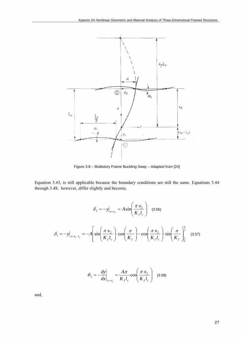
Figure 3.8 – Multistory Frame Buckling Sway – Adapted from [24]

quation 3.43, is still applicable because the boundary conditions are still the same. Equations 3.44 Ethrough 3.48, however, differ slightly and become,

⎟⎟⎞

⎜⎜⎛

=−==xx

xAy 2

2 sinπ

δ (3.56)

⎠⎝ cf lK2

⎥⎥⎦

⎤

⎢⎢⎣

⎡⎟⎟⎠

⎞⎜⎜⎝

⎛⋅⎟

⎟⎠

⎞⎜⎜⎝

⎛−⎟

⎟⎠

⎞⎜⎜⎝

⎛⋅⎟

⎟⎠

⎞⎜⎜⎝

⎛−=−=

−=fcffcf

lxx KlKx

KlKxAy

c

ππππδ sincoscossin 22

12

(3.57)

⎟⎟⎠

⎞⎜⎜⎝

⎛=−=

= cfcfxx lKx

lKA

dxdy 2

2 cos2

ππθ (3.58)

nd, a

27


⎥⎥⎦

⎤

⎢⎢⎣

⎡⎟⎟⎠

⎞⎜⎜⎝

⎛⎟⎟⎠

⎞⎜⎜⎝

⎛+⎟

⎟⎠

⎞⎜⎜⎝

⎛⎟⎟⎠

⎞⎜⎜⎝

⎛=−=

−= fcffcfcflxx KlKx

KlKx

lKA

dxdy

c

πππππθ sinsincoscos 221

2

(3.59)

imilarly, for frame deflections according to sway buckling modes, where the moment of inertia of the Sbeams is constant at each level, and all columns in the frame have the same moment of inertia, the rotations at each end of a beam are equal both in magnitude and direction. As such, 6=b and the rotation, for example, at node 2 can be expressed as,

2

22 6 b

b

EIlPδ

θ = (3.60)

ubstituting P for the critical buckling load and taking 2δ fromS 3.56, 3.60 becomes

⎟⎟⎠

⎞⎜⎜⎝

⎛⎟⎟⎠

⎞⎜⎜⎝

⎛=

cffc lKx

KlAG 2

2

22 sin

6ππθ (3.61)

roceeding in the same manner for P 1θ ,

⎥⎥⎦

⎤

⎢⎢⎣

⎡⎟⎟⎠

⎞⎜⎜⎝

⎛⎟⎟⎠

⎞⎜⎜⎝

⎛+⎟

⎟⎠

⎞⎜⎜⎝

⎛⎟⎟⎠

⎞⎜⎜⎝

⎛−=−=

−= fcffcfclxx KlKx

KlKx

lAG

dxdy

c

ππππθ sincoscossin

6221

12

(3.62)

liminating 2θ from 3.58 and 3.61, and 1θE from 3.59 and 3.62, one obtains two expressions for

clfKx2cotπ (similarly to 3.53 and 3.54). Eliminating this and simplifying the result one obtains the

that is used in AISC,

final expression

( )

f

ff

K

KGG

KGG

π

ππ

tan6

36

21

2

21

=+

−⎟⎟⎠

⎞⎜⎜⎝

⎛

(3.63)

.1.4. COMPARISON BETWEEN CODES OF PRACTICE

the present form, immediate comparison of the K-Factor expressions is impossible because of the

3

Indifferent nature of the distribution coefficients (EC3), the relative flexibility ratio (EC2) and relative stiffness ratios (AISC) – which in essence are the same, but one will differentiate between them for the

28


sake clarity. However, consider 3.63 as a transformation of 3.22 from a nominal distribution coefficient to an effective distribution coefficient

=⎟⎠⎞

⎜⎝⎛+⎟

⎠⎞

⎜⎝⎛

⎟⎠⎞

⎜⎝⎛

⋅⋅

=⎟⎠⎞

⎜⎝⎛+⎟

⎠⎞

⎜⎝⎛

⎟⎠⎞

⎜⎝⎛

=

∑∑

∑

∑∑

∑

i ibeamcolumns

columns

i ibeamcolumns

columnsi

lI

lI

lI

EE

lI

lI

lI

,,

44

ααη

∑∑

∑

∑∑

∑

⎟⎠⎞

⎜⎝⎛+⎟

⎠⎞

⎜⎝⎛

⎟⎠⎞

⎜⎝⎛

=⎟⎠⎞

⎜⎝⎛+⎟

⎠⎞

⎜⎝⎛

⎟⎠⎞

⎜⎝⎛

=

i ibeamcolumns

columns

i ibeamcolumns

columns

lEI

lEI

lEI

lEI

lEI

lEI

,,

4

4

44

4

βα

(3.63)

one divides by ik iηIf one obtains,

=

⎟⎠⎞

⎜⎝⎛+⎟

⎠⎞

⎜⎝⎛

⎟⎠⎞

⎜⎝⎛⋅

⎟⎠⎞

⎜⎝⎛

⎟⎠⎞

⎜⎝⎛

=

⎟⎠⎞

⎜⎝⎛+⎟

⎠⎞

⎜⎝⎛

⎟⎠⎞

⎜⎝⎛

⎟⎠⎞

⎜⎝⎛

⎟⎠⎞

⎜⎝⎛

=

∑∑

∑

∑

∑

∑∑

∑

∑

∑

i ibeamcolumns

columns

i ibeam

columns

i ibeamcolumns

columns

i ibeam

columns

i

i

lEI

lEI

lEIl

EIl

EI

lEI

lEI

lEI

lEI

lEI

k

,

,

,

,

4

4

4

4

β

β

β

β

η

41

4

44

41

,,

, +⎟⎠⎞

⎜⎝⎛⋅

⎟⎠⎞

⎜⎝⎛

=⎟⎠⎞

⎜⎝⎛

⎟⎠⎞

⎜⎝⎛+⎟

⎠⎞

⎜⎝⎛

=

∑

∑

∑

∑∑

i ibeam

columns

i ibeam

i ibeamcolumns

lEI

lEI

lEI

lEI

lEI

ββ

β

.64)

ttending to 3.26,

(3

a

( )i

ii

iii

k

kk

ηη

η

−⋅=⇔

⇔⋅⎟⎠⎞

⎜⎝⎛ +=

14

41

(3.65)

29


ves a relation between distribution coefficients and relative flexibility ratio, used in

differences between the K-Factors given by EC3 (dashed lines)

Equation 3.65 giboth EC3 and EC2, respectively.

In Figures 3.9 and 3.10 one can see the and EC2 (continuous lines) for nonsway and sway cases, respectively.

Figure 3.9 – Comparison of K-Factors given by EC2 and EC3 in NonSway

Figure 3.10 – Comparison of K-Factors given by EC2 and EC3 in Sway

zing the data, one can assess the maximum difference between the two codes of practice, which Analyfor nonsway is about 3% and for sway about 15%. Since both procedures are a result of equations adjusted to transcendent expressions (3.23, 3.24, 3.27 and 3.28), one can state that the observed differences are a result of numerical adjustments - EC3 being overall the most conservative.

30


Proceeding in the same way as 3.64 and 3.65, one can derive the relation between AISC’s nodal stiffness ratios and it’s counterparts in EC2 and EC3. Table 3.1 summarizes all of these relations.

Table 3.1 – Relations Between Nodal Stiffness Ratios of EC3, EC2 and AISC

EC3 EC2 AISC

EC3 - i

ii k41+

=ηk4

4

0bGi

i+

=ηGi

EC2 ( )i

iik

ηη−⋅

=14

- 0b

Gk i

i =

AISC ( )i

ii

bG

ηη−⋅

=140 ii kbG 0= -

Since the AISC expressions for K-Factors are implicit, a practical alternative for comparing different results is to solve the equation as a function of one of its end restraints ratios for a given K-Factor, as presented in 3.66 and 3.67, derived from 3.31 and 3.32 respectively.

Nonsway

⎟⎟⎟⎟⎟

⎠

⎞

⎜⎜⎜⎜⎜

⎝

⎛

−+⎟⎟⎠

⎞⎜⎜⎝

⎛

⎥⎥⎥⎥

⎦

⎤

⎢⎢⎢⎢

⎣

⎡

+

⎟⎟⎟⎟⎟

⎠

⎞

⎜⎜⎜⎜⎜

⎝

⎛

−−⋅

=

f

f

f

f

f

f

f

K

KK

G

K

K

K

KG

G

π

ππ

π

π

π

π

tan1

2

2

2tan

tan1

212

2

1

1

2 (3.66)

Sway

f

f

f

f

f

K

KK

G

K

KG

G

π

ππ

π

π

tan6

36tan

6

2

1

1

2

−⎟⎟⎠

⎞⎜⎜⎝

⎛

+

= (3.67)

Proceeding similarly for EC3 one obtains,

31


Nonsway a

acbb2

42

2−±−

=η (3.68)

where,

055.0=a

111.014.0 η+=b

fKc −++= 211 055.014.05.0 ηη

(3.69)

and,

Sway( )

( ) 2.012.06.08.0

12.08.01

112

112

2−−−

−+−=

ηη

ηηη

f

f

K

K(3.70)

As for EC2, deriving from expression 3.27 yields,

Nonsway

1

1

21

1

2

2

45.01

42

1

45.01

4

45.0

kk

Kk

kK

kf

f

++

−

−

++

⋅= (3.71)

Since 3.28 defines the K-Factor as a maximum of two expression, one has to apply the same procedure to both and, when plotting the comparison, judge which one translate into the highest K-Factor.

Sway

Expression A

1

1

1

1

2

11

2

1

11

kk

Kk

kK

kf

f

++

−

−

++

= (3.72)

Expression B ( )

( )11.0

11.02

1

12

2−−

−=

f

f

Kk

kKk (3.73)

32


With the expressions that have been presented (3.66 through 3.73), and using the relations of table 3.1, one can obtain the following results (Figures 3.11 through 3.13).

Figure 3.11 – Comparison Between Codes of Practice for Nonsway

Figure 3.12 – Comparison Between Codes of Practice for Sway - { }0.3;0.2;3.1∈fK

33


Figure 3.13 – Comparison Between Codes of Practice for Sway - { }0.15;0.10;0.8;0.7∈fK

An important aspect of the figures plotted above is that conclusions as to the difference in K-Factors, as those made for Figures 3.9 and 3.10, are not immediately possible because what is displayed is in fact the difference in nominal distribution coefficients iη . Since the variation in a iη is not representative of the variation in the K-Factor – for instance in nonsway,

3.1599.00 21 =→=∧= fKηη and 1.1273.00 21 =→=∧= fKηη therefore a difference of

120% in iη corresponds to a variation of 18.2% in the K-Factor. What can be inferred, however, is the relative significance of each curve, i.e. whether one is more conservative than the other, and under what conditions those assertions are valid. As such, the constructed charts serve as qualitative basis for analysis.

From the figures presented, one can validate the conclusion that the expressions given by each code of practice are very closely related and are not equal because EC3 and EC2 are numerical approximations of the exact formulation of the problem, which correspond to AISC’s curves.

Figure 3.11 charts the comparison for nonsway between EC3, EC2 and AISC for three values of K-Factors – 0.55; 0.7; and 0.85. The main conclusion from the analysis of this chart is that EC3 is overall more conservative than EC2 – same conclusion reached for Figure 3.9 – and EC2 goes as far as being non-conservative. But since the differences between EC2 and EC3 are at the most 3% for these cases, this is of negligible significance.

In Figures 3.12 and 3.13 one can see the comparison for sway between EC3, EC2 and AISC. Perhaps this is the most interesting case to analyze because of the two expressions given by EC2. As one can observe there is a discontinuity in the EC2 - A curve that gives way to EC2 –B, each with different

34


curvatures. As the K-Factor increases, EC2 – A loses its weight in the expression entirely – see Figure 3.12, in which EC2 – A was plotted purposefully. EC3 for small values of K- Factor (< 3)

is conservative. For values higher than 3 it becomes non conservative – see Figure 3.12. This fact in itself is not very alarming because as one can see from Figure 3.10, for high K-Factors, EC3 and EC2 practically coincide and since both are upper and lower boundaries, the difference between EC3 and the exact formulation is negligible. In EC2, however, problems arise precisely where the difference seen in Figure 3.10 is most critical (yielding errors between 10-15%). This area can be observed in Figure 3.12 for

0.3=fK

0.3=fK where it is clear that the curve EC2 – B diverges from the exact solution as

iη increases. This aspect is critical because it is on the unsafe side, even though this translates, for example, in a difference between 2.91 and 3.33 in K-Factor values.

In conclusion, the best numerical adjustment for K-Factor values is the EC3 expressions, yielding minimal errors and being overall the most conservative. When it is not conservative the errors are found to be negligible.

3.2. STIFFNESS REDUCTIONS FACTORS

The need for stiffness reduction factors arises from the demand to predict the behavior of a structure in which nonlinear effects have an increased significance in its performance. These effects can be fundamentally of two different natures: geometric nonlinearity and material nonlinearity. The geometric behavior comprises the second order effects induced by loss of stiffness in the presence of axial loads in structural members, as well as additional internal forces raised from the deformed shape of the structure. Material nonlinearity includes a variety of phenomena such as: material plasticity, cracking, creep, shrinkage, relaxation and temperature.

Since a correct nonlinear analysis, which has all of these variables taken into account, can be very time consuming for common purposes, the practical design of these structures calls for simplifications in the way the analysis is made in order to most effectively simulate the nonlinear behavior. Where a fire assessment isn’t present, material nonlinearity can be modeled essentially by three parameters: plasticity, cracking and creep.

The following subsections will present the recommendations of different codes of practice as a way of dealing with this issue.

3.2.1. EUROCODE 2

Eurocode 2 proposes three methods of carrying out nonlinear analysis. The first is through the full nonlinear material and geometric analysis – the General Method. The latter two are simplified methods: the Nominal Stiffness Method and the Nominal Curvature Method.

The Nominal Curvature Method, according to the code, is particularly ‘adequate for isolated elements subject to a constant normal force and a defined effective length’ and gives a ‘nominal second order moment based on a displacement which, in itself, is based on the effective length and an estimated maximum curvature’. Due to the restrictive range of application of this method, an in depth analysis will not be made.

35


As for the Nominal Stiffness Method it, in essence, is based in finding an equivalent stiffness that simulates the nonlinear geometric and material behavior, and has a wider range of application.

Compressed Structural Elements

For this purpose, the code of practice presents the following expression which, it stipulates, can be used for any cross section,

sssccdc IEKIEKEI + =

cdE

(3.74)

where, is the design value of the concrete modulus of elasticity given by expression 3.75, the concrete’s cross section moment of inertia, the design value of the reinforcement steel modulus of elasticity, the reinforcement steel’s moment of inertia in relation to the cross section’s centroid,

a coefficient that takes into account nonlinear effects, and a coefficient that takes into account the contribution of the reinforcement in the overall nominal stiffness.

cI

sE

sI

cK sK

2,1cm

cE

cmcd

EEE ==

γ(3.75)

cK and can be obtained through two sets of expressions (one more elaborated, one more simplified). The first set, which is valid only if the geometric reinforcement ratio is higher than 0,2%, is as follows,

sK

1=sK

efc

kkKϕ+

=1

21 (3.76)

where,

201

ckfk = (3.77)

20,01702 ≤⋅=λνk (3.78)

36


Ed

Eqpef M

Mt

0

00 ),( ⋅∞= ϕϕ (3.79)

and,

il0=λ (3.80)

efϕ is the effective creep coefficient, the characteristic compressive strength of the concrete; ckf ν

the reduced normal load; λ the slenderness of the element; ),( 0t∞ϕ the final creep coefficient; the first order moment in the quasi-permanent combination of action; the first order

moment in ultimate limit state; l the effective length; the radius of gyration. EqpM 0 EdM 0

0 i

2If the slenderness of the element is not defined, one can use an alternate expression for k ,

20,030,02 ≤⋅=νk (3.81)

The second set, which is valid only if the geometric reinforcement ratio is higher than 1%, is as follows,

0=sK

efcK

ϕ5,013,0

+= (3.82)

Eurocode 2 states that this second set, might be adequate for a quick preliminary analysis, followed by a more rigorous assessment using 3.76.

Long term nonlinear material effects are particularly influenced by creep, as one can see from 3.76 and 3.82. The method that Eurocode2 uses for accounting this phenomenon is to modify the extensions in the constitutive law of the concrete, as seen in Figure 3.14

37


Figure 3.14 – Simple Way to Accounting for Creep Effects – From [22]

Structural Elements With Negligible Axial Load – Adjacent Elements

For redundant structures, the effect of the adjacent elements influences the overall performance of the structure. However, the evaluation of the stiffness reduction factors in these cases cannot be done through the application of the expressions presented in 3.76 or 3.82, because the axial load in these elements is negligible and thus the effects of geometrical nonlinearity are minimal. Eurocode 2 allows as a simplification to consider the cross sections as fully cracked throughout its length. In order to evaluate these reductions let us consider the rectangular beam cross-section presented in Figure 3.15.

Figure 3.15 – Fully Cracked Elastic Cross-Section

38


Given that is the cross section’s height, the cross section’s width, the reinforcement’s area, the distance from the top fiber to the reinforcement’s centroid, and

h b Asd x as the distance from the top fiber to the neutral axis, one can define the following quantities,

dx

=ξ (3.83)

c

s

EE

=α (3.84)

bdAs=ρ (3.85)

Since this analysis is elastic, it can be easily proven that the neutral axis’s position is only a function of the ratio between modulus of elasticity (equation 3.84) and its geometric reinforcement ratio (equation 3.85) and is given by the following expression,

0222 =−+ αραρξξ (3.86)

Through the manipulation of equations 3.83 to 3.86 and disregarding , one can reach the conclusion that the fully cracked moment of inertia of the cross-section is,

dh −

( ) ⎥⎦

⎤⎢⎣

⎡−+= 2

33 1

3ξαρξbdI cracked (3.87)

as opposed to,

⎥⎦⎤

⎢⎣⎡ +=

41213 αρbdIuncracked (3.88)

The stiffness reduction factor then is nothing but the relation between the two,

( )

4121

13

23

αρ

ξαρξ

+

−+==

uncracked

cracked

II

r (3.89)

39


Figure 3.16 illustrates these reductions for a concrete grade of C30/37, including the partial safety coefficient presented in 3.75, for short term loading.

Figure 3.16 – Stiffness Reduction Factors For a Rectangular Cross-Section Beam in Short Term Loading

3.2.2. EUROCODE 4

Eurocode 4 [3] allows for the consideration of material and geometric nonlinearity in a way similar to the Nominal Stiffness Method, that Eurocode 2 proposes for compressed structural elements. It, however, gives two expressions for the definition of the effective flexural stiffness, depending on the purpose of the analysis that is performed. If one’s purpose is to ascertain the relative slenderness of a column, or to determine the internal forces in a second order linear elastic analysis, one should use expressions 3.90 and 3.91, respectively.

( ) ccmssaaeff IEIEIEEI 6,0++= (3.90)

( ) ( ccmssaaIIeff IEIEIEEI 5,09,0, )++= (3.91)

where, is the design value of the structural steel’s modulus of elasticity, the structural steel’s section moment of inertia, the average value for the concrete’s modulus of elasticity.

aE aIEcm

Long term effects are also taken into account similarly to EC2, as is expressed in equation 3.92

( )( )0,, ,1

1ttNN

EEEdEdG

cmeffc ϕ⋅+= (3.92)

40


where, is the part of the normal force that is permanent; the design normal force, and EdGN ,

)EdN

( 0, ttϕ the creep coefficient at time t as estimated by Eurocode 2.

3.2.3. ACI

This code of practice proposes the following expressions for an effective stiffness in structural elements subject to compression,

d

sscc IEIEEI

β++

=1

2,0(3.93)

d

cc IEEI

β+=

14,0

(3.94)

Long term loading is account for with dβ+1 where dβ for nonsway is defined by the ratio of maximum factored axial sustained load to the maximum factored axial load, and for sway frames as the maximum factored sustained shear within a story to the maximum factored shear in that story. In equation 3.93, this term is divided by both the concrete and reinforcement contributions. Although this fact is, in itself, difficult to comprehend, the code’s commentary offers the explanation that ‘this reflects the premature yielding of steel in columns subjected to sustained load’.

For elements with negligible axial force it suggests the following reductions to their moments of inertia:

Table 3.2 – Flexural Stiffness Reduction Factors For Structural Elements With Negligible Axial Load

Structural Element Reduction Factor

Beams 0,35

Flat Plates and Flat Slabs 0,25

ACI also offers an expression to account for loss of stiffness in a composite cross-section and is as follows,

sxsxd

cc IEIE

EI ++

=β1

51(3.95)

where, is the value of the structural steel’s modulus of elasticity, and the structural steel’s cross section moment of inertia.

sxE sxI

41


3.2.4. BRIEF COMMENTARY

As one can see from 3.93, for short term loading, the reduction factor for concrete that ACI proposes is equal to 0,2 and if one examines the expression 3.78 is precisely the upper bound that Eurocode 2 stipulates. It however does not directly relate to the reduction factor because in Eurocode 2 also depends on the concrete grade – see equation 3.76 and 3.77. Directly comparable are the more simplified expression 3.94 and 3.82, where the Eurocode presents itself as being more conservative than ACI – with 0,3 for a reduction factor rather than 0,4.

cK

Long term loadings are similarly handled by Eurocodes 2 and 4, as can be seen from 3.79 and 3.92. Between the European codes and ACI there is a very clear difference which lays in the fact that the American code does not explicitly consider a creep coefficient. In expressions 3.93 and 3.94, it is as if the creep coefficient is always equal to 1.

3.3. AMPLIFICATIONS DUE TO SECOND-ORDER EFFECTS

Amplification factors are simplified ways to account for additional internal forces that arise from second order effects. As it will be shown, there is great affinity between codes of practice in this area – namely Eurocodes 2, 3 and 4 and ACI and AISC. They all are a function in some way or another of the ratio of an applied load to the critical buckling load – see 3.96.

crPP

−1

1(3.96)

This expression can be used as an approximation to estimate the maximum mid span deflection of a beam-column under three conditions of symmetrical loading (concentrated load at mid span; uniform transverse loading; and two equal end moments)[25] and can be derived through an expansion in a Fourier trigonometric series of the deflection curve. If the values of crPP aren’t large – less than 0,6 – than the expression has negligible errors – less than 2% [25].

There are, however, other alternatives to this ‘classic’ evaluation, as is the case of CEB’s Model Code 90[6] which calculates the amplification not through the relation between the applied load and it’s corresponding critical load, but through the estimation of a second order displacement or rotation. Eurocode 2, also supplies a formulation that allows for a different approach, which will be presented ahead.

3.3.1. EUROCODE 2

Eurocode 2 proposes two sets of amplification factors: the first being a moment amplification; the second a horizontal force amplification.

42


Moment Amplification

Using Eurocode’s notation, consider equation 3.96

⎥⎥⎥⎥

⎦⎢⎢⎢⎢

⎣−

+=1

10

Ed

BEdEd

NN

MM β⎤⎡

EdM 0

(3.97)

where is the first order moment; β a coefficient that depends on the distribution of the first and second order moments (admitted to have a sinusoidal configuration) and is equal to equation 3.98; the critical buckling load based on nominal stiffness (see subsection 3.2.1); the axial design load.

BN

EdN

For isolated elements of constant cross-section and axial load,

0

2

cπβ = (3.98)

where is a coefficient that depends on the distribution of the first order moment (0c 80 =c for a constant first order moment; for a parabolic distribution; 6,90 =c 120 =c for a symmetric triangular distribution, etc.).

For elements not subject to transverse loading, different first order moments at the extremities, and , can be replaced by an equivalent first order moment, ,as is expressed in 3.99,

02M

01M e0M

0201020 4,04,06,0 MMMM e ≥+= (3.99)

In cases where the before mentioned conditions do not apply, 1=β usually constitutes ‘a reasonable simplification’ and 3.97 becomes 3.100, an expression that mimics 3.96.

B

Ed

EdEd

NN

MM

−=

1

0

(3.100)

43


Horizontal Force Amplification

The horizontal force amplification factors are a way to conduct a global second order analysis and its effects on the structure. To this effect Eurocode 2 allows the use of two expressions, the first one being identical to equation 3.96, and is presented in equation 3.101.

BV

EdVEdH

FF

,

,,

1−

EdHFF 0,=

EdHF ,

(3.101)

where, is the amplified fictitious horizontal force; the first order horizontal force due to

wind or imperfection loads, for example; the total vertical load in the bracing and braced

elements; the global critical buckling load using nominal stiffness values.

EdHF 0,

EdVF ,

BVF ,

Eurocode 2, also allows the horizontal amplification factor to be determined in a different way. Consider equation 3.102,

EdH

EdH

EdHEdH

FF

FF

0,

1,

0,,

1−=

(3.102)

where is a horizontal fictitious force that produces the same flexural moments as the vertical

load acting on the deformed shape of structure caused by the first order forces and calculated

using nominal stiffness values.

EdHF 1,

EdHF 0,

This expression (3.102) arises from a step by step analysis where the effects of the structure’s deformation and subsequent increments in internal forces due to vertical load (simulated through equivalent horizontal forces) are successively added and form a geometric series after a few steps. If one assumes that that happens from the very first step then the sum will take the form of equation 3.102. This hypothesis requires that the stiffness values that represent the final stage of deformation are used on all steps. If not, the expression can be modified to accommodate this fact by adding more terms to the calculation sequence, for example:

EdH

EdH

EdHEdHEdHEdH

FF

FFFF

2,

3,

2,1,0,,

1−++=

(3.103)

44


3.3.2. EUROCODE 3

Eurocode 3 allows the use of an amplification factor defined by,

crα11−

1(3.104)

where, crα is the factor by which the design loading would have to be increased to cause elastic instability in a global mode. One can immediately infer that crcr PP=α1 and therefore 3.104 is equal to 3.96. This factor is allowed to be used in the analysis of multi-storey frames when all stories have similar distribution of vertical loads, horizontal loads and frame stiffness with respect to the applied storey shear forces.

It also provides an approximate formula for the determination of this load factor,

⎟⎟⎠

⎞⎜⎜⎝

⎛⎟⎟⎠

⎞⎜⎜⎝

⎛=

EdHEd

Edcr

hVH

,δα (3.105)

where is the design value of the horizontal reaction at the bottom of the story to the horizontal load and fictitious horizontal loads; is the total design vertical load on the structure on the bottom of the story;

EdH

EdV

EdH ,δ is the inter-story drift when the frame is loaded with horizontal loads and fictitious horizontal loads, applied at each floor level; h the storey height.

3.3.3. EUROCODE 4

According to Eurocode 4, ‘Second-order effects may be included indirectly by using a first-order analysis with the appropriate amplification’[3]. For isolated structural elements, it allows the first order design bending moment to be multiplied by a factor given by, EdM k

effcr

Ed

NN

k

,

1−=

β(3.106)

where, is the critical buckling load for the relevant axis and corresponding flexural stiffness

(equation 3.91) with the effective length taken as the columns length and effcrN ,

β an equivalent moment factor given by Table 3.3.

45


Table 3.3 – Factors β For The Determination Of Moments To Second-Order Theory – From [3]

Moment distribution Moment factors β Comment

First-order bending moments from member

imperfection or lateral load:

0,1=β

EdM is the maximum bending moment within the

column length ignoring second-order effects

End moments:

r44,066,0 +=β

but 44,0≥β

EdM EdrMand are the end moments from first-order or second-order global analysis

As one can see from 3.106, the amplification factors is fairly similar to 3.96, apart some corrections made to account for loading conditions.

3.3.4. ACI

Nonsway Frames

For nonsway frames, ACI defines an amplification factor nsδ as,

0,1

75.01

≥−

=

cr

u

mns

PP

Cδ

(3.107)

where is a coefficient by which one multiplies the maximum absolute moment in the element to obtain an equivalent constant moment throughout the beam, akin to 3.99 (see equation 3.108). and the factored axial load. The critical load here is calculated for each member and its corresponding effective length and equivalent stiffness (obtained either by 3.93 or 3.94 or 3.95).

mC

uP

4,04,06,02

1 ≥+=MMCm (3.108)

46


Sway Frames

ACI for these types of frames allows two types of expressions. The first is presented in equation 3.109

0,11

≥=sδ

75.01−

∑∑

cr

u

PP (3.109)

The 0,75 factors (both in the nonsway and sway expressions), the code’s commentary states[4], is a stiffness reduction factor. Alas, this fact is not very clear to the author for it suggests that the stiffness reductions are considered twice in the amplification factor. Adding to which, the critical load is evaluated as the sum of the individual column’s buckling load as opposed to the more intuitive global critical load as Eurocode 2 uses in 3.101. However, it is not to say that the approach behind the calculation of the magnification is different. The fundamental traits are very much similar to the one’s expressed in 3.96.

The second is a variation of the simplified method also present in Eurocode 3, as one can see from 3.110 and 3.111

0,11

1≥

−=

Qsδ (3.110)

where,

crcus

ou

lVP 1Δ

Qα

== ∑(3.111)

and is the inter story drift; V the total horizontal story shear; and l the story’s height. oΔ us c

2B

3.3.5. AISC

The amplified first-order elastic analysis provided by AISC is based on two types of amplifiers: for second order effects caused by displacements between brace points; and to account for effects caused by displacements of braced points.

1B

The required second-order flexural strength, , and axial strength, , are determined by equations 3.112 and 3.113 respectively.

rM rP

ltntr MBMBM 21 += (3.112)

47


ltntr PBPP 2+= (3.113)

1B is defined as follows,

0,1

11

1 ≥−

=

e

r

m

PP

CB

α (3.114)

and , 2B

0,1

1

1

2

2 ≥

−

=

∑∑

e

nt

PP

Bα (3.115)

where, is the same coefficient that ACI uses (apart some sign conventions); mC α a partial safety

coefficient; the elastic critical buckling resistance of the member for nonsway; the elastic

critical buckling resistance for the story in sway buckling; with subscripts ‘nt’ meaning ‘no lateral translation of the frame’ and ‘lt’ meaning ‘

1eP ∑ 2eP

only lateral translation of the frame’.

∑ 2eP is allowed to be calculated through two ways: one the sum of the critical buckling load of each

member of the story (similar to ACI’s equation 3.109); the other by the following expression,

H

Me

LHRP

Δ= ∑∑ 2 (3.116)

where, is the inter-story drift; the story shear produced by the lateral forces used to

compute the drift; the story’s height; and a coefficient equal to 1,0 in braced-frame systems and 0,85 for a moment-frame and combined systems, unless a larger values are justified by analysis.

HΔ ∑ HL MR

If one takes 3.114 and replaces it into 3.113, it yields an expression that is very similar to the one offered by ACI (equations 3.110 and 3.111) and consequently akin to Eurocode 3’s equations 3.104 and 3.105. Although the approach to the magnifications is the same, their application differs, since AISC quite clearly separates the effects caused by loadings that do not produce any lateral translations (where the factor is applied) and those that do (where the factor is applied) – see equations 3.112 and 3.113.

1B 2B

48


3.3.6. MODEL CODE 90

Model Code 90 offers an alternative way for evaluating second-order effects in sway frames, which is applicable to uniformly distributed horizontal and vertical loads and constitutes a special form of the P-Δ method. Consider Figure 3.17

Figure 3.17 – Representation Of The Simplified Method For Assessing The Maximum Displacement Due To

Second-Order Effects – From [6]

Also, let us define as a design horizontal load, a design vertical load, an incremental horizontal design force;

SdH SdV SdHΔ

aα the slope associated with global imperfections; the first order top displacement of the frame due to horizontal forces ;

( SdHa' )SdH ( )SdVa'

''a first order top displacement of

the frame due to the vertical load on the deformed shape; the second order top displacement of the frame;

SdV''α the second order slope; and l as the height of the frame.

The procedure to calculate ''α is as follows:

lHa

la Sd

a)(''''

ΔΔ++= αα (3.117)

Through a direct proportion one can estimate lHa Sd )(' ΔΔ through,

( )

lHa

xHxH

lHa Sd

Sd

SdSd ')('

∑∑Δ

=ΔΔ

∑Δ

(3.118)

Equation 3.118 represents the fact that the incremental rotation is equal to the rotation caused by the first order moment in proportion to the incremental second-order moment . ∑ xH Sd xH Sd

49


Since,

SdSd VH ''α=Δ (3.119)

Then equation 3.117 becomes,

lHa

xHV

la Sd

Sd

Sda

)(''''''∑

∑++=α

αα (3.120)

And, therefore,

lHa

xHV

la

Sd

Sd

Sd

a

)('1

'

''

∑∑−

+=

αα (3.121)

The effective horizontal load, , is therefore equal to, efSdH ,

SdSd

SdSdSdefSd H

HV

VHH ⎟⎟⎠

⎞⎜⎜⎝

⎛+=+= ''1'', αα (3.122)

Where ⎟⎟⎠

⎞⎜⎜⎝

⎛+

Sd

Sd

HV''1 α constitutes the magnification factor.

As a note, in chapter 5 an attempt at an extension of this method from 2D to 3D is made and a small shift in nomenclature is made so that the text becomes more understandable. For example displacements become a δ and axis X, that represents the direction of the height of the structure, becomes Z.

3.3.7. BRIEF COMMENTARY

The bulk of amplification factors that were summarized in this section fall behind the same classical approach – the ratio between the applied axial load and the corresponding critical buckling load. All of the codes of practice under analysis are at their very core equal to one another, except for Model Code 90 and one procedure allowed by Eurocode 2.

50


There are, however, some differences on how to calculate the critical buckling loads in sway modes, and the most pronounced difference is brought forth by AISC that completely separates loads that cause floor translation from those that do not.

3.4. CONCLUSIONS

In this Chapter, three different aspects that relate to nonlinear geometric and material analysis were analyzed under the perspective of several codes of practice: effective lengths, stiffness reductions and amplification factors.

With respect to effective lengths, it was found that, throughout the different codes of practice that were comparable (Eurocode 2 and 3, ACI and AISC), the manner with which each length was calculated, although different in ways of evaluating end restraints, yields the same results, apart some numerical errors.

As for stiffness reduction factors, two different features present themselves – the assessment of short term and long term loading. For short term loading, ACI and Eurocode 2 have some similarities, although the European code offers a more sophisticated way of calculating the stiffness reductions that involves variables such as the applied reduced axial load, the slenderness of the member and the concrete grade that is used – none of which are an issue for ACI. For long term loading, the approach behind its consideration is very similar for Eurocodes 2 and 4, but differs from ACI’s as the American code considers the effect of creep to be applied not only to concrete but also to the reinforcement part of the cross section’s flexural stiffness.

Amplification factors were found to be, at their very core, almost identical between all the codes of practice that were analyzed, except for one – Model Code 90. The basic assumption that is used to calculate the magnification, is based on an extrapolation of an amplification derived from an isolated beam-column under specified symmetrical loads. Corrections are made available in some codes for types of loading that do not coincide with the scope of the theoretical derivation. There are, however, alternatives for the calculation of the magnifications, such as the one proposed by Model Code 90.

The following Chapter will deal more specifically with the criteria for the application of the several aspects that were discussed in this one. It will address issues like the limitations associated with effective lengths, the code requirements for stiffness reduction (the way which they were derived and a comparative analysis of several sets of numerically modeled beams and columns) and the potential for the use of visco-elastic models for a comprehensible structural analysis.

51


52


4 GUIDELINES FOR PRACTICE

6. 4.1. EFFECTIVE LENGTH

Although may the theory behind the concept of effective lengths be very much established, its application time and again proves to be of difficult interpretation and often leads to miscalculations. It is such that in certain countries Eurocode 3’s national annex prohibits the use of effective lengths to calculate critical loads[26].

Being the most effective way to illustrate this problem, consider the following worked example, adapted from [27] and presented in Figure 4.1.

Figure 4.1 – Worked Example – Load Cases i) and ii); Nonsway a) and Sway b)

53


Let us calculate the buckling length (using Eurocode 3) and global critical buckling loads for each example:

a-i)

From 3.22,

0;75,0

5,15,0

21 ==+

= ηη

lI

lI

lI

Which from 3.23, yields . From a global elastic stability analysis one obtains 64,0=fK22308,2 lEIPcr π= which from 3.3, yields 66,0=fK , very similar results.

a-ii)

Basing the effective length calculation solely on an intuitive symmetrical deformed shape, the K-Factor is, in fact, the same for a-i) being 64,0=fK . In a global analysis, however, the critical load is

found to be 22245,1 lEIPcr π= and since the applied load is different in each column the has to be, necessary different buckling lengths for each one, per equation 3.3: ,leftfKK

63,0= and

. 90,0, =rightf

b-i)

From 3.22,

0;50,0

5,15,1

21 ==+

= ηη

lI

lI

lI

Which from 3.23, yields . From a global elastic stability analysis one obtains 23,1=fK22660,0 lEIPcr π= which from 3.3, yields 23,1=fK .

54


b-ii)

y on an in the same for b-i) bei

Again, basing the effective length calculation in solel tuitive anti-symmetrical deformed shape, the K-Factor is, in fact, ng 23.1=fK . In a global analysis, however, the

critical load is found to be 22439,0 lEIPcr π= and since the applied load is different in each has to rycolumn the be, necessa different buc one, per equation 3.3:

e

kling lengths for each07,1, =leftfK and 51,1, =rightfK .

Having arrived at these results one might be inclined to say this method suffers from the fact that it only seems to work for load and stiffness distributions so that the critical load of the column is reached simultaneously to the frame’s buckling load. But there is a fundamental assumption in these calculations: the assumed deformed shape. In fact, for case loadings a-i) and b-i) a symmetrical and anti-symmetrical deformed shape is quite true. But for case loadings a-ii) and b-ii), this is not the case because one column has higher axial load then the other, leading to an asymmetrical loss of stiffness – the left being more flexible than the right. This automatically leads to more rotation in th upper node of the left column than in the right one and, as such, the assumptions used to calculated iη cannot be the same for both: a-i) and a-ii); and b-i) and b-ii). The pa erameter α , then, cannot be obtain by considering equal and opposit tations of the beam ( 0,5ee end ro α = ) or equal end rotations both in magnitude and in direction ( 1,5eα = ) but should be calculated using a relation between the end rotations like the o e givenn by 3.41 , which

quation 4.1, that applies to the case that was analyzed (with equal column moments of inertia) – [28].

equation for use in Eurocode 3 should be used along with a reference value 0b of 4.

The fundamental misconception then is that nonsway frames always have a symmetrical buckling mode for a symmetrical arrangement of stiffness and, that sway frames always have an anti- symmetrical buckling mode for a symmetrical arrangement of stiffness. This, as it was pointed out, is untrue and consequently leads to miscalculations. The evaluation of effective lengths must therefore always be expressed in terms of end rotations given by its true buckling mode, be that nonsway or sway, which takes into account not only the arrangement of stiffness in the structure but also asymmetries in the loading and interaction effects between members. One must first determine the structure’s buckling mode to perform this analysis correctly. For simple cases, however, expressions can be derived that take this effect into account, such as those in e

⎟⎟⎠

⎞⎜⎜⎝

⎛+

++=

left

rightleftf P

Pc

cK 121

5,731,

(4.1)

where

columnbeam

Applying 4.27 and its equivalent for the right column, y

beamcolumn

lIlI

c = (4.2)

ields 06,1, =leftfK and 51,1, =rightfK ,

almost identical to the values given by the global analysis.

55


4.2. STIFFNESS REDUCTION FACTORS FOR REINFORCED CONCRETE AND COMPOSITE ELEMENTS

4.2.1. REINFORCED CONCRETE STRUCTURAL ELEMENTS WITH NEGLIGIBLE AXIAL LOAD – ADJACENT

ELEMENTS

This sub-section will discuss the required stiffness reduction factors for elements with negligible axial load, in ultimate limit state. To accomplish this one must first present the basic assumptions used in the numerical modeling of such elements. To this effect, consider the following beam [29]

Figure 4.2 – Spacial Arrangement Of a Tested Beam [mm] – According to [29]

and, the following material properties, [29]

Table 4.1 – Material Properties – According to [29]

Concrete Compressive Strength (N/mm2)

Reinforcement Bars (φ16)

Yield Strength (N/mm2)

Tensile Strength (N/mm2)

Young Modulus (kN/mm2)

38,5 368 568 200

The numerical tests were performed using the computer software Diana [30] and, as such subject to its numerical models. The formulation of reinforced concrete nonlinear behavior which was used for these trials (Total Strain –Fixed Cracking – Brittle in Tension and Ideal in Compression) can be seen as an extension of theory of elasticity models to account for the behavior of concrete cracking, which is usually associated with a nonlinear elastic model in compression [31]. Fixed cracking models admit that once the concrete reaches its maximum tensile strength, a zone appears where cracking has taken place with a direction that is perpendicular to the maximum stress and remains with that direction throughout the loading [31]. As soon as the limit stress is reached, the variation of the normal stress within this zone can be specified to account for tension softening, tension stiffening effects or, more conservatively, that the stress falls immediately to zero (Brittle in Tension). The nonlinear behavior in compression was, in this case, assumed to be elasto-plastic which was deemed to be a reasonable approximation for the purposes of this work.

As one can see Figure 4.3, the modeled beam fits quite well with the experimental data.

56


Figure 4.3 – Comparison Between Experimental and Numerical Modelling

As such and defining as the criteria for attaining an ultimate limit state (ULS) the reaching of the reinforcement steel’s yield strength or the concrete’s ultimate extension (3,5 ‰), one can estimate the element’s deformed shape for this state.

Since cracking and plasticity do not occur equally throughout the span of the beam, one has to define also a criterion to approximate the effective flexural stiffness. One way to do so, is estimate the deformed shape in ULS by the theoretical deformations given by the well known relation,

( )( ))('')(''

xyxMEI

EIxMxy −=⇔−= (4.3)

where by adjusting the values of the curvatures one obtains a fair approximation of EI (yielding 2R values of over 98%).

The main difficulty with doing this approximation is that a normal least-square method for the estimation of the parameters that define the deformation, do not necessarily comply with the exact solution given by the beam’s boundary conditions. For example, take 4.4 as the law that defines a simply supported beam’s deformed shape, for uniform transverse loading (Figure 4.4),

57


Figure 4.4 – Simply Supported Beam Under Uniform Transverse Loading

( ) 432 exdxcxbxaxy ++++= (4.4)

If one is to apply a least square fit without regard to the beam’s boundary conditions the most common outcome would be to have and , which is untrue and distorts the purpose of using such a method. The most common boundary conditions are expressed in expressions 4.5, 4.6 and 4.7 (pinned, fixed and no support and loading, respectively)

0≠a 0≠c

02

2

==dx

ydy (4.5)

0==dxdyy (4.6)

03

3

2

2

==dx

yddx

yd(4.7)

Consider Figure 4.5 that presents the different types of constraints analysed.

58


Figure 4.5 – Different Types Of Constraints Analyzed For a Beam Under Uniform Transverse Loading

Table 4.2, on the other hand, represents the values that the different parameters in equation 4.4 have to have so that they respect the boundary conditions of each type of constraints.

Table 4.2 – Parameter Values

a b c d e

CO1 0 3el 0 el2− e

CO2 0 0 2el el2− e

CO3 0 0 25,1 el el5,2− e

CO4 0 0 26el el4− e

Furthermore, one can approximate the deformed shape merely by changing the values of e so that it fits the least square criterion. Differentiating 4.4, and substituting into 4.3, yields,

21262)(

exdxcxMEI++

−= (4.8)

To demonstrate the effectiveness of such a method consider Figure 4.6 that represents the deformed shape of a beam (CO3) for ULS and its corresponding least square fit,

59


Figure 4.6 – Deformation Of A Beam For A CO3 Type Of Constraints

Having discussed the methodology to estimate the effective flexural stiffness, one must now make a series of numerical tests. The principal variable to be evaluated is naturally the reduced moment of the beam, and, as such, the modeled beams were designed according to current standards to take this factor into account. For example, let us say that beam X is designed for a reduced moment of 0,2 ( 2,0=μ ) and, as such, per equilibrium equations, has a mechanical reinforcement ratio of 0,226 ( 226,0=ϖ ). To that ratio corresponds exactly a reinforcement area and that is exactly the amount that was used in the modeling of the beam. For redundant cases, such as CO2 and CO3, the reinforcement area was calculated so that the critical sections would yield at the same time. Then beam X is modeled and an effective stiffness estimated. The reduction factor is then calculated as,

sA

Uncracked

Estimated

EIEI

r = (4.9)

The modeled beams were all calculated for a concrete grade C30/37 and reinforcement steel S500, and Table 4.3 presents the most pertinent dimensions of each set,

60


Table 4.3 – Cross-Section Dimensions and Beam Length For Each Set [m]

b h d l

Set 1 0,2 0,45 0,41 5

Set 2 0,3 0,7 0,66 7

Set 3 0,2 0,35 0,31 3

Set 4 0.3 0,5 0,46 7

Set 5 0,5 0,29 0,25 5

Set 6 0,6 0,24 0,20 5

Set 7 0,6 0,27 0,23 7

Each set was modeled for four types of constraints and for five reduced moments ( { 3,0;25,0;2,0;15,0;1,0∈ }μ ), tallying up to 140 modeled beams (7x4x5). Figures 4.6 to 4.9 illustrate the results that were obtained.

Figure 4.7 – Stiffness Reduction Factors for Constraints CO1

61




62



As one can see, the general tendency to diminish the reductions for growing values of reduced moment (for there is also a growth in the mechanical reinforcement ratio that contributes the section’s overall flexural inertia) is verified. Also, one can observe a fairly wide range of values for each type of constraint and a given reduced moment. To this effect let us turn the attention to Table 4.4 that summarizes the most important statistical quantities in the results that were obtained.

Table 4.4 – Statistical Quantities Associated With The Results

μ r stdvσ vc μ r stdvσ vc

CO1

0,1 0,211 0,029 13,7%

CO3

0,1 0,127 0,017 13,6% 0,15 0,298 0,038 12,9% 0,15 0,182 0,025 13,6% 0,2 0,372 0,048 12,8% 0,2 0,233 0,033 14,1% 0,25 0,433 0,056 13,0% 0,25 0,288 0,041 14,3% 0,3 0,478 0,060 12,6% 0,3 0,341 0,050 14,5%

CO2

0,1 0,107 0,014 12,7%

CO4

0,1 0,214 0,027 12,4% 0,15 0,152 0,019 12,4% 0,15 0,294 0,039 13,2% 0,2 0,196 0,027 13,6% 0,2 0,375 0,049 13,0% 0,25 0,242 0,030 12,4% 0,25 0,441 0,059 13,5% 0,3 0,286 0,036 12,5% 0,3 0,508 0,065 12,9%

where, r is the average of the reductions, stdvσ the standard deviation and the coefficient of variation.

vc

63


From Table 4.4, one can observe fairly high standard deviations in some cases (0,065 for example). However, if one is to analyze the distribution with a dimensionless quantity, such as the coefficient of variation (that represents the ratio between the standard deviation and the average) in may conclude that they are somewhat similar, ranging in an interval from 12,4% to 14,5%.

If one is to analyze the results through the calculated averages, one can, not only establish a comparison of the estimated reduction factors between types of constraints, but also compare it with code requirements as presented in Chapter 3. To this effect, observe Figure 4.11

Figure 4.11 – Comparison Between Averages And Code Requirements

The differences that come from the consideration of different end restraints are immediately evident in Figure 4.11. A very useful conclusion that one can make from this figure is that the degree of redundancy seems to be a factor of considerable importance. Simply supported and cantilever beams have almost identical reductions but are very dissimilar for constraints CO2 and CO3. This effect can be explained if one imagines several stages of loading of a beam fixed at both ends. In a first stage the beam is uncracked throughout its length and has stiffness provided not by its cross-section but also by the inability of its extremity sections to rotate. In a second phase, the beam starts to crack at the extremities, losing stiffness not only through the loss of some of its effective cross-section but also through the increasing ability for the sections immediately adjacent to the extremities to rotate. This is the cause for a higher reduction in redundant members.

With regard to code requirements, since most beams are designed for a reduced moment of 0,25, ACI’s required value falls fairly between the two most extreme values (CO1 and CO2). If one is to consider for an adjacent element a unidirectional slab, since its design is conditioned only by one direction (i.e. no interaction between stresses from another direction), the assumption that these results are applicable to those cases is considered to be a legitimate approximation. As such, since the design

64


value commonly used in the design of these elements is 0,15, ACI’s reduction factor also falls in the interval defined by the two most extreme values – although more close to the limit imposed by CO1.

Although from the analysis of Figure 4.11 one is inclined to dismiss Eurocode 2’s reduction factors as being on the unsafe side, one must first consider how they were obtained. The geometric reinforcement ratio in Figure 3.16, was converted in a mechanical reinforcement ratio and from this ratio a corresponding reduced moment was calculated. However, one must keep in mind that the graph portrayed in Figure 3.16 was obtained with the basic assumption that dh − was a quantity sufficiently small to be disregarded. If one is to compare the plotted Eurocode 2 reduction factors in Figure 4.11 with Figure 4.7 one would reach the conclusion that the EC2 reduction factors are very closely related to Set 2’s reductions, precisely the Set that has the highest ( )dhh − ratio. This being said, Eurocode 2’s requirements do not seem so far on the unsafe side as it may appear in Figure 4.11, but follows the same trend values as a stiffness reduction factor of a simply supported beam, which may not be the most appropriate.

4.2.2. COMPRESSED STRUCTURAL ELEMENTS

In addition to material nonlinearity, these cases present themselves with an additional factor – geometric nonlinearity. Similarly to the elements with negligible axial load, stiffness reduction factors are evaluated through the approximation of the deformed shape by a least square fit. In this case, however, a direct adjustment is made due to the fact that the flexural stiffness is directly part of the deformed shape – as given by equation 4.10 [25], in correspondence with Figure 4.12.

Figure 4.12 – Bending of a Beam-Column by End Moments

( ) ( )⎟⎟⎠

⎞⎜⎜⎝

⎛ −−

−+⎟⎟

⎠

⎞⎜⎜⎝

⎛−=

lxl

jlxlj

PM

lx

jljx

PMxy

sinsin

sinsin 12 (4.10)

where,

EIPj = (4.11)

65


This analysis was made with the help of two computer programs Fagus and Pyrus[32-33]. The first was developed with the purpose of cross sectional calculations, namely interaction curves (N-MX-My) , moment-curvature (M-ϕ) curves and moment-flexural stiffness curves (M-EI) of both reinforced concrete and composite steel-concrete sections. For a given state of strain the program associates a selected stress-strain relation to the cross-section – the stress-strain curve used in these analysis is the one proposed by Eurocode 2. Then, internal forces are determined by integration of stresses along the section. Since in the tests that were performed what was given was a particular state of external forces and not a state of strain, the program reaches a solution through an iterative process that involves incrementing the sections strain diagram by a Newton-Raphson procedure until internal forces and external forces are equilibrium.

The second program, Pyrus, performs a nonlinear material and geometric analysis through an iterative process that stops when a satisfactory tolerance is reached and is based on a nonlinear finite element method. Geometric nonlinearity is accounted for by establishing equilibrium conditions in the deformed structure - including effects of large deformations. Material nonlinearity is taken into account by performing an integral of the cross-section stresses for a given state of strain – parallel to Fagus. The criteria used to evaluate a column’s ultimate load were: achieving the cross-section’s ultimate load (i.e. reaching limit strains for the concrete or steel) or achieving a collapse due to instability. The schematic arrangement of the modeled columns is presented in Figure 4.13.

Figure 4.13 – Schematic Representation of the Modeled Columns

Reinforced Concrete Columns

Eurocode 2 stiffness reductions factors, presented in Chapter 3, were estimated for columns that have equal end eccentricities, both in magnitude and direction (i.e. 121 =ee )[22]. Evaluations of ACI’s expression for stiffness reduction factors have been made also by using this method[34]. Since a column rarely experiences pure flexure, an investigation to the effect of three different end eccentricities have been made – 121 =ee ; 121 −=ee ; 5,021 −=ee .

66


Another factor that plays a key role in this evaluation is not the end eccentricities but its relative eccentricity, a dimensionless parameter as expressed in 4.12:

he

ff

bhP

ff

bhPe

ff

bhP

ff

bhM

yd

cd

yd

cd

yd

cd

yd

cd

===22

νμ

(4.12)

Figure 4.14 presents the range of tested relative eccentricities, in an intuitive way – spanning across an interaction diagram for rectangular cross-sections.

Figure 4.14 – Span Of Tested Eccentricities On An Interaction Diagram – Diagram from [35]

Then, if a cross-section is designed for a given a set of relative eccentricities, a particular point in the interaction diagram is defined by the mechanical reinforcement ratio of the section. Three distinct values of mechanical reinforcement ratio were tested: 2,0=ϖ , 4,0=ϖ , and 6,0=ϖ , that for the columns that were analyzed (C30/37 and S500) represent roughly 1, 2 and 3% of geometric reinforcement ratio.

Also, the cross-section that was used for these calculations consists of a 30x30 cm square with 3 cm of cover. Two sets of slenderness were also modulated by considering two different heights: ml 3= and

ml 6= that correspond roughly to 35=λ and 70=λ , respectively. Accounting for all of these

67


variable mns (14 eccentricities the tally goes up to 252 colu s x 3 types of eccentricities x 3 mechanical reinforcement ratios x 2 different column heights). The bulk of the research is too extensive to be comprehensively presented in this document. However, sufficient information to understand the key findings of the numerical trials is presented in the proceeding figures – 4.15 to 4.18.

Figure 4.15 – Stiffness Reduction Factors For 2,0=ϖ and 3=l

here EC2 represents in expression 3.76, for short terms loading; and ACI the concrete reduction w cKin expression 3.93.

Figure 4.16 – Stiffness Reduction Factors For 2,0=ϖ and 6=l

68


Figure 4.17 – Stiffness Reduction Factors For 4,0=ϖ and

rom Figures 4.15, 4.16 and 4.17 one can immediately reach four conclusions: the first that the

eductions for low slenderness values

er slenderness values, approximations given by Eurocode 2 do not follow the same pattern of

f one is to examine it’s behavior

portant conclusion is that the ratio between the end eccentricities does influence a great

3=l

FEurocode 2 expressions are generally conservative; the second that they approximate the concrete reduction more effectively for lower slenderness values; the third that ACI’s reductions are on the unsafe side if one is to examine the whole span of e/h values; and finally that the difference in end eccentricities plays a key role in the definition of the reductions.

Eurocode 2 expressions mimic fairly well the decay in stiffness ras one can see from Figures 4.15 and 4.17. There is, however, an appreciable discrepancy between these expressions and the modeled values for low relative eccentricity values. This is more visible in Figure 4.17 and suggests that for this range and with these slenderness values, the dominating collapse behavior is dictated by material nonlinearity and, as such, the concrete reductions are significantly higher.

For highdecay as the modeled columns. However, they still offer a reasonable degree of approximation for e/h values in an interval between 0,1 and 0,7 – most common values in design application [34]But for other values the proposed equations appear to be fairly conservative.

ACI’s reductions seem to be, in loose terms, on the unsafe side, but ifor the range for which the equations were developed e/h<0,4 [34]one can observe more reasonable differences.

The other imdeal the concrete reduction factors, leading overall to smaller reductions (higher values). The differences between these relationships for different slenderness values can be seen in Figure 4.18. For the sake interpretation, only 121 =ee and 121 −=ee are plotted.

69


Figure 4.18 – Stiffness Reduction Factors For 2,0=ϖ

As one can observe in Figure 4.18, there is a tendency for columns with 121 =ee to have lower reductions as the slenderness increases. This fact is counter-intuitive but can be explained by the tendency for the column to destabilize before the material reaches its full resisting capacity and, therefore, the need to reduce the stiffness is less if the predominant behavior is geometric in nature. For 121 −=ee , the column has less tendency for instability and, hence, the predominant behavior is material in nature. This conclusion is all the more compelling for low e/h values, as can be seen in Figure 4.18.

Composite Steel-Concrete Columns

The analysis for composite columns is a little more difficult to perform as section characteristics are not easily evaluated in terms of dimensionless parameters as can be done with reinforced concrete sections. Thus, the calculations that have been done necessarily express the nature of a particular section, as opposed to a family of similar sections (as is done for RC sections by reduced axial loads and moments). Also, a fundamental assumption was taken in this analysis that consists of considering that the ratio e/h is representative of the relationship between loading and stiffness reductions – akin to distribution presented in Figure 4.14.

Since the stiffness reduction factors in Eurocode 4 present variables reducing both the concrete and the structural and reinforcement steel’s part of the flexural stiffness, the evaluation was made by analysing the reduction of the cross-sections as a whole (see – equation 4.9).

Three cross-sections were analyzed as were two types of slenderness (roughly corresponding to 35=λ and 70=λ ) and three types of end eccentricity ratios, tallying up to 252 columns.

The following figures show the geometric characteristics of the three cross sections that were modeled.

70


a) b)

c)

Figure 4.19 – Composite Cross-Sections Analyzed – a) Section 1; b) Section 2; c) Section 3

As for the material characteristics, the concrete grade used was C30/37, the reinforcement steel S500 and the structural steel S355.

Figure 4.20 – Stiffness Reduction Factors For Section 1

71




As one can see, slenderness effects are much more pronounced in these types of columns. From Figure 4.20, one can immediately infer that for low values of e/h, the reductions greatly vary for the behavior is dictated by either material nonlinearity (lower slenderness) of geometric nonlinearity (higher slenderness). Fact that by itself is not very surprising, for it was also observed in reinforced concrete columns, but to verify that for 121 −=ee and 5,021 ee = − this also happens, when in these conditions the column is much less prone to instability, is indeed a significant result. This behavior, however, is less evident for sections 2 and 3 where, for the referred end eccentricity ratios, geometric

72


nonlinearity is less pronounced – more in consonance with the reinforced concrete columns. Since the models have comparable slenderness values, the only difference in the whole analysis seems to point out that the geometric arrangement of the cross-section plays a significant role.

With respect to code requirements, one can conclude that Eurocode 4 is much more aware to the fact that different type of end eccentricity ratios are a relevant issue, as one can see from Figures 4.20, 4.21 and 4.22. The Eurocode’s approximation is more closely related to values of 121 −=ee and

5,021 −=ee , fact that is all the more visible for higher slenderness values. For cases where material nonlinearity is the dominant behavior, the required limit falls short of an accurate prediction and is on the unsafe side. However, since this fact was only analyzed for concrete encased sections, and since effects of concrete confinement are not taken into account, this statement can hardly be considered conclusive and applied to all types of composite cross sections. Thus, this analysis serves primarily to make assertions on a qualitative base.

ACI’s predictions seem to be in accord with 121 =ee types of ratio and appear to be conservative in most cases, especially for relevant slenderness values.

4.3. POTENTIAL FOR THE USE OF VISCO-ELASTIC MODELS IN NONLINEAR MATERIAL AND GEOMETRIC ANALYSIS

All of the stiffness reduction factors that were analyzed in the preceding sub-sections share a common characteristic: they are applicable for short term loadings. Since deformation is a critical aspect for geometric nonlinear, certainly creep and possibly shrinkage effects play a key role in the structure’s overall performance.

4.3.1. THEORETICAL BACKGROUND

Strains in concrete can be fully accounted for by the sum of several components of deformation each responsible by a different type of phenomenon – see equation 4.13.

( ) ( ) ( ) ( ) ( )ttttt cTcscccic εεεεε +++= (4.13)

where, ( )tcε is the total concrete strain, ( )tciε the instantaneous strain due to loading, ( )tccε the creep component of strain, ( )tcsε the shrinkage component of strain; ( )tcTε the thermal component of strain; and t time.

Setting aside the thermal component, and if one is to consider a constant stress, the concrete stress is given by

( ) ( )( )

( )( ) ( ) (ttttEt

tEt

t csc

c

c

cc εϕ )σσ

ε ++= 00

0

0 , (4.14)

73


If the stress varies over time, the principle of superposition applies and equation 4.14 becomes,

( ) ( )( ) ( ) ( ) ( )tdtJtEtt cs

c

c

cc ετ

ττστσε

τ+

∂∂

+= ∫00

0 , (4.15)

( )τwhere ,tJ is the creep function, defined by the creep coefficient and modulus of elasticity, both of which are time dependent.

The creep coefficient itself is a very hard thing to evaluate for it depends on many factors. The main factors have in essence two distinct natures: intrinsic (concerning the concrete itself) and extrinsic (concerning exterior factors). Table 4.5 presents a summary of these factors as done by [36] but not all of them are used in the prediction of the creep coefficient.

Table 4.5 – Summary of Factors That Can Be Used to Define The Creep Coefficient

Intrinsic Factors Extrinsic Factors Aggregate Type Age At First Loading

A/C Ratio Age of Sample Air Content Applied Stress

Cement Content Characteristic Strength at Loading Cement Type Cross-Section Shape

Concrete Density Curing Conditions Fine/Total Aggregate Ratio (Mass) Compressive Strength at 28 Days

Slump Duration of Load W/C Ratio Effective Thickness

Water Content Elastic Modulus at Age of Loading Elastic Modulus at 28 Days

Relative Humidity Temperature

Time Drying Commences

The most common way of computing this phenomenon is through the use of Kelvin chain models. Consider Figure 4.23,

74


Figure 4.23 – Kelvin Model

where η is the dashpot viscosity, dσ the stress in the dashpot and sσ the stress in the spring.

Also consider the following equations,

ds σσσ += (4.16)

εσ Es = (4.17)

dtd

dεησ = (4.18)

Substituting 4.18 and 4.17 in 4.16 one obtains,

dtdE εηεσ += (4.19)

If one considers that a constant stress is applied then the solution of the differential equation 4.19 assumes the form of,

( ) ( )( )

teCtEt

t λσε −+= 1

0

0 (4.20)

where

ηλ E

= (4.21)

75


Since the stress is constant, the variation of the strain must necessarily be constant as well. This provides an initial condition because it illustrates that the strain cannot suffer jumps between the instant in which the model is unstressed and instant in which the stress is applied. This implies that

( ) 00 =+tε [37] then becomes, 1C

( )( )0

01 tE

tC

σ−= (4.22)

and, hence,

( ) ( )( )

( )( )010

0 ttetEt

t −−−= λσε (4.23)

As such, the creep function can also be expressed as,

( ) ( )( )( )011,

00

ttetE

ttJ −−−= λ(4.24)

If one is to consider a chain model like Figure 4.24, the creep function becomes equation 4.25,

Figure 4.24 – Kelvin Chain Model

( ) ( )( )( )∑

=

−−−=n

i

tt

i

ietE

ttJ1 0

0011, λ

(4.25)

For variable stress over time equation 4.15 still applies and 4.25 becomes

( ) ( )( )( )∑

=

−−−=n

i

t

i

ieE

tJ1

11, τλ

ττ (4.26)

Also, one can see the creep function as,

76


( ) ( )( ) ( )

( )( )011,,

00

00

ttetEtE

ttttJ −−−== λϕ

(4.27)

And, therefore,

( ) ( )01, 0ttett −−−= λϕ (4.28)

So, in other words, the creep coefficient defines the dashpot’s viscosity.

4.3.2. WORKED EXAMPLE AND VERIFICATION

The following example is based on experimental data presented in reference [18].

Creep coefficient and shrinkage strains are calculated through Model Code 90’s predictions. For creep these predictions are almost identical to Eurocode 2’s expressions but for shrinkage are somewhat different. Since further development and comparison of these predictions would result in a somewhat extensive presentation, far beyond the purpose of this work, the author suggests the consultation of the referred standards [1, 6].

The software used in this numerical modeling is Diana [30]. Other material nonlinearity effects such as cracking is accounted for through the use of multidirectional fixed cracking model. This consists of smeared cracking model with strain decomposition (i.e. the total strain is equal to the sum of two independent components: the elastic strain and the crack strain) and allows for the consideration of multiple cracks with various directions at the same sampling point [38] – see Figure 4.25.

Figure 4.25 – Multidirectional fixed cracking model [38]

The tensile behavior of the concrete was considered to perform under a softening curve proposed by Hordijk [39] – see Figure 4.26

77


Figure 4.26 – Hordijk Softening Curve – Taken from [38]

where, the stress in the crack normal to the plane of the crack, ultimate strain of the crack

normal to the plane of the crack, the concrete’s tensile strength, the concrete’s fracture energy, and the estimated crack bandwidth (i.e. an idealized bandwidth within which the cracking occurs at a constant strain; depends on the type and refinement of the finite element model).

crnnσ cr

ultnn,ε

fGtfh

The finite element model that was used consists of eighty, three-node, two-dimensional Timoshenko beam type of elements, integrated throughout its length by 2 Gauss points and throughout it height with 11 Simpson points.

The experiment is done on a slender column, and the geometric configuration is presented in Figure 4.27.

Figure 4.27 – Details and Testing Arrangements For The Columns [mm] – Taken from [18]

78


The loading details are presented in Table 4.6 and material properties can be observed in Table 4.7

Table 4.6 – Loading Details [18]

Specimen C1 C2 C3 C4 C5

Te (mm) 50 50 50 50 50

Be (mm) 50 25 0 -25 50

Load (kN) 70.0 70.0 80.0 80.0 85.0

Table 4.7 – Material Properties [18]

cmf 28,cE 28,ctf υ γ fG sE syf

29,3 MPa 35,4MPa 2,2 MPa 0,2 23,5 kN/m3 75 N/mm 200 GPa 500 MPa

Figures 4.28 to 4.32 show the principal results that were obtained.

Figure 4.28 – Results for Column C1

79




80




As one can see from the figures that have been shown there is a strong correlation between the observed and the modeled deflections curves. The model correctly predicts the behavior of the column when subject to various moment gradients. As a note, the software that was used to model these columns (Diana) does not allow an updated Lagrangean formulation to beam elements; only solids, plane strain elements, axisymmetric elements and interface elements can use it[38]. Perhaps this is the

81


reason for a somewhat under estimation of the displacement values above, but since the applied load is fairly lower then the critical buckling load, this effect was considered to be relative importance. Therefore, the performed analysis can only be made using these types of elements in this particular program (which will require a great deal of elements) or by another program that has this type of visco-elastic formulation.

4.4. CONCLUSIONS

In this Chapter issues like the implementation of effective lengths, stiffness reduction factors for both uncompressed and compressed elements, and the potential for the use of visco-elastic models in long term nonlinear geometric and material analysis are discussed.

With regard to effective lengths, their implementation is analyzed and the potential for miscalculations using this method is highlighted using a simple example where the simple assertion that the buckling mode assumes a particular shape (symmetric and anti-symmetric) leads to results that are notably inconsistent with a global analysis. This is due to the wrong assumption of the buckling mode shape that, for an asymmetrical loading, will not lead to a symmetric or anti-symmetric buckling mode, depending on if the structure is nonsway or sway.

The main conclusion that can be made from what is presented about stiffness reduction factors is that the effect of end restraints is without a doubt a relevant issue and should be taken into account in code requirements. This aspect is of sizeable importance with respect to non-compressed structural elements for the analysis that was made suggests that higher reductions occur precisely when these elements are redundant in nature – and most of these types of elements in frames are precisely that. For compressed structural elements, the effect of end restraints is particularly sensitive to their end eccentricity ratio. For eccentricity ratios of 121 −=ee these reductions can be diminished and correspond to moment gradients typical of a column in a framed structure.

As for the use of visco-elastic models, the usefulness of these methods, having validated its predictions, is their application to structures with a low buckling load factor to evaluate their long term effects on its overall performance. That is precisely a study that is recommended for future development.

In the next Chapter an attempt is made at an extension of Model Code 90’s amplification method, as is presented in Chapter 3, so that it might be able to tackle the three-dimensional nature of a structure’s spatial arrangement.

82


5 3D APPROACH FOR THE ASSESSMENT OF SECOND ORDER EFFECTS – AN EXTENSION OF MC90 SIMPLIFIED METHOD

5. 5.1. INTRODUCTION

The assessment of second order effects in a global structural analysis can be done through the amplification factors that were discussed in Chapter 3. However, the application of these magnification factors, with regard to three-dimensional structures, usually involves two two-dimensional analyses, one per perpendicular plane. This results in two independent analyses that in a three-dimensional perspective may not be the most suitable, for the added stresses from second order effects in one direction, can result in stresses in the other perpendicular direction due to the structure’s torsional response. It is in this context that an attempt at an extension for the assessment of these effects is made in order to incorporate three-dimensional behavior. To this end, the method proposed by Model Code 90 [6], presented in sub-section 3.3.6, seems to be an excellent candidate for such extension.

Consider the following figure,

a) b)

Figure 5.1 – a) Deformed Structure and Its Approximation; b) Spatial Consideration of The Approximation

83


In Figure 5.1 a), one can see the deformed shape of a basic structure and, as is assumed by MC 90, an approximation of the deformation of each column that consists of a linear variation throughout the column’s length ( ) from the top displacement of the column (l δ ) to its foundation (in red). This approximation can be better seen and understood in Figure 5.1 b), where α represents the distortion ( lδ ) and β the angle that the projection of the deformation makes in plane XY with the axis X.

Let us make some simple remarks on the projections represented in Figure 5.1 b) and consider the projection of displacement δ on axis X,

βδδ cos=x (5.1)

Dividing both members by the column length, one obtains,

βααβδδcoscos =⇔= x

x

ll(5.2)

and, as such, the projection of the distortion in plane XZ can be calculated merely by multiplying global distortion the cosine of angle β . Proceeding similarly for the Y axis returns,

βαα sin=y (5.3)

This result suggests that the distortion of each individual column can be evaluated by two independent planes, regardless of the distortion being first-order or second-order in nature.

The main difficulty associated with the three-dimensional nature of this problem, is that the deformation due to imperfections (associated to a buckling mode) may not have the same direction as the deformation that results from the actual loading of the structure. Therefore, if one is to tackle this problem in a three-dimensional point of view, one must first find a way to consider both of these effects in the analysis. With the conclusion that each column can be analyzed through two independent directions, if one is to consider each factor (imperfection and loading) regardless of each other, which for a linear analysis is a valid assumption, and if one is to work on them through their projections on two independent planes, then the final result can be derived simply by the sum of their effects in their projections. To better understand this, consider Figure 5.2, where all the displacements represent the top deformation of the column and iδ the displacement due to imperfection, ( )VSDH'δ the first order displacement associated to the vertical load on the deformed structure (imperfections), SDV ( )SDH'δ the first order displacement associated to the horizontal load , SDH ( )VSDH''δ the second order displacement associated to the vertical load on the deformed structure (imperfections), SDV ( )SDH''δ the second-order displacement associated to the horizontal load and 'SDH 'δ the total top displacement of the column.

84


Figure 5.2 –Projection of the First and Second Order Displacements of the Column in Plane XY

Let us now consider an analysis per axis and, thus, add all the respective components in, for example, the X axis, as is expressed in 5.4.

( ) ( ) ( ) ( ) θδζδγδϖδβδδ cos''cos''cos'cos'cos'' SDVSDSDVSDix HHHH ++++= (5.4)

From 5.4, one immediately acknowledges that angles ζ and θ are an important factor in this relation. However, in light of Model Code 90’s method, these angles need not be determined or, more precisely, can be determined but indirectly. Consider, for example a cantilever column whose top displacement is represented in Figure 5.3.

Figure 5.3 –Projection of the First and Second Order Displacements of a Cantilever Column in Plane XY in a

Simplified Loading

85


Because of the difference of the column’s inertia in plane X and Y, even if a loading is such that the first order displacement is carried out in a 45 degree angle, the presence of axial force (vertical load

) can be seen as producing an equal effect on the structure through two equal horizontal forces in both directions ( and ) which inexorably leads to a displacement that is carried out, not in the same angle than the previous 45 degrees, but in a naturally higher angle that one calls

SDV

xSDH ,Δ ySDH ,Δθ . If one

takes the projection of the second order displacement in the X axis, according to the Model Code 90’s approach, it can be estimated by a proportion involving other displacements in the same axis and the forces that lead to those displacements. This assumption results in the following equality,

( ) ( )xSD

xSD

SDSD H

HH

H ,,

º45cos'cos'' Δ=

δθδ (5.5)

thus, circumventing the need to calculate the angle θ .

This, of course, also applies to angle ζ in Figure 5.2, and applying this concept to Equation 5.4, in correspondence with Equation 3.117, one obtains,

( ) ( ) +++= γδϖδβδδ cos'cos'cos'' SDVSDix HH

( ) ( ) ∑∑∑∑⋅Δ

⋅+⋅Δ

⋅+ zH

zHHzH

zHH

xSDxSD

SDxSD

xVSD

VSD,

,,

,

cos'cos' γδϖδ

(5.6)

Attending to 3.119,

( ) ( ) +++= γδϖδβδδ cos'cos'cos'' SDVSDix HH

( ) ( ) ∑∑∑∑ ⋅+

⋅+ SD

x

xSD

SDSD

x

xVSD

VSD VlzH

HV

lzHH ''cos'''cos'

,,

δγδδϖδ

(5.7)

Which yields,

( ) ( )=⎟

⎟⎠

⎞⎜⎜⎝

⎛

⋅+

⋅− ∑∑∑∑ SD

x

xSD

SDSD

x

xVSD

VSDx V

lzHH

VlzH

H ''cos'''cos'''

,,

δγδδϖδδ

( ) ( )δ β δ ϖ γδ cos'cos'cos SDVSDi HH ++=

(5.8)

and finally, the final second-order displacement in the X axis is given by,

86


( ) ( )( ) ( )

⎟⎟⎠

⎞⎜⎜⎝

⎛

⋅+

⋅−

++=

∑∑∑

zHH

zHH

lV

HH

xSD

SD

xVSD

VSDSD

SDVSDix

,,

cos'cos'1

cos'cos'cos''

γδϖδ

γδϖδβδδ

(5.9)

Proceeding similarly for the Y axis, yields,

( ) ( )( ) ( )

⎟⎟⎠

⎞⎜⎜⎝

⎛

⋅+

⋅−

++=

∑∑∑

zHH

zHH

lV

HH

ySD

SD

yVSD

VSDSD

SDVSDiy

,,

sin'sin'1

sin'sin'sin''

γδϖδ

γδϖδβδδ

(5.10)

As such, the equivalent second-order horizontal forces are equal to,

SDx

xSDxeqSD Vl

HH''

,,,δ

+= (5.11)

and,

SDy

ySDyeqSD Vl

HH''

,,,

δ+= (5.12)

Having arrived at this stage, one must now interpret the way in which these equations should be, implemented - which is not the most immediate. Consider, for example, a case where geometrical imperfections aren’t considered on the analysis and that a structure, like the one portrayed in Figure 5.1 a), is subject to a torsional moment applied by two horizontal forces on two diametrically opposed nodes. In this situation, one might be inclined to say that for the columns which have no directly applied load, expressions 5.9 and 5.10 do not have meaning for they tend to zero. However, this only an apparent limitation for all the external loads can be applied to the structure through equivalent loads, in several ways. Two immediately come to mind: transforming the external loads in three independent loads (horizontal load in the X axis; horizontal load in the Y axis; and a torsional moment) applied at the shear centre of the floor, and distribute those loads according to each member’s stiffness; or, by applying the loads in a normal first order analysis, and obtaining the whole structure’s internal forces, one can, at each member, interpret its shear forces as external equivalent horizontal loads, thus applicable to equations 5.9 and 5.10. The latter procedure presents itself as the most practical and will be used in the examples that are presented ahead.

The methodology, then, can be comprised in a series of steps that are presented in the flow chart in Figure 5.4.

87


Figure 5.4 – Flow Chart Of The Proposed Methodology

Another detail that deserves further consideration is the application of global geometric imperfections to the structure. In the examples that are developed ahead, the imperfections were given according to the structure’s first buckling mode, be that a torsional buckling mode, or a pure translational one, and, as such, the deformed shape is scaled so that the maximum top displacement of a column reflects a distortion of 1/200. This, however, is a simplification of the problem for there are other two factors that play a significant role. The first that, the distortion is usually an upper bound of values that is used for design purposes, because, for example, Eurocodes 2 and 3[1-2] allow for the use of reduction coefficients that depend on the structure’s height and number of elements per floor. The second that, even though for high vertical loads the structure tends to buckle in the first critical mode, regardless of the direction of lateral loading, for design purposes (vertical loads sufficiently lower than the buckling load) if imperfections are taken to be only in to be the first mode, there may be cases where it is not conservative to consider the imperfections only this mode – especially if the critical loads of the first, second, or even third mode are very close together. It is, therefore, recommended that the imperfections be given not only according to the first buckling mode, but also other modes that are considered to be relevant in the analysis.

5.2. EXAMPLES

The examples that are presented ahead were solved with the aid of the computer program Robot Structural Analysis [40]. However, from known experience, this software may not be this most adequate for nonlinear geometric structural analysis and, as such, the values that are brought forth are merely indicative of the behavior of the proposed equations, because any errors that occur, for example, in the determination of the structure’s critical load, will affect in the same way the vertical

88


load that was used in the proposed formulas for what is used is a critical load factor. Hence, it is highly recommended that the proposed extension be put to test and validated with the aid of more powerful and reliable software.

5.2.1. STRUCTURE 1

Consider Figure 5.5, which represent loading number one of Structure 1, perpendicular the structure’s buckling mode.

a) b)

Figure 5.5 – Structure 1 – Loading No. 1 – a) Loading; b) Buckling Mode

Structure 1 has one floor (3 m), one Bay in the X direction (3 m), one Bay in direction Y (3 m), and all columns and beams are in structural steel, hot-rolled section HEB240. Lastly, actual relative displacements on the floor level are taken into account by introducing a concrete 30cm slab (C30/37).

Table 5.1 presents the principal results from the proposed methodology, for a critical load factor equal to 10.

Table 5.1 – Structure 1 – Load No.1 – Principal Results For a Critical Load Factor of 10

1st Order Linear Elastic (LE1) Proposed Method (PM) Nonlinear Analysis (NL)Column Node MY (kNm) MX (kNm) MY (kNm) MX (kNm) MY (kNm) MX (kNm)

1 Bottom 32,13465 6,637733 33,20231 7,402137 33,33985 7,097551 Top ‐28,0357 ‐6,35361 ‐28,9691 ‐7,0821 ‐29,2015 ‐7,10556

2 Bottom 32,09644 6,58409 33,15969 7,346032 32,96042 7,023587 Top ‐27,9591 ‐6,22457 ‐28,8837 ‐6,94813 ‐28,8141 ‐6,96459

3 Bottom 31,97055 6,56358 33,03379 7,325519 33,15227 7,048977 Top ‐27,8591 ‐6,2052 ‐28,7837 ‐6,92875 ‐29,0145 ‐7,00828

4 Bottom 32,00876 6,658243 33,0764 7,42265 32,87077 7,13225 Top ‐27,9357 ‐6,37298 ‐28,8691 ‐7,10147 ‐28,7892 ‐7,16582

89


Table 5.2 represents the relative differences between analysis,

Table 5.2 – Structure 1 – Load No. 1 – Relative Differences For a Critical Load Factor of 10

(LE1‐NL)/LE1 (PM‐NL)/PM

Col. N. MY MX MY MX

1 Bot. ‐3,8% ‐6,9% ‐0,4% 4,1% Top ‐4,2% ‐11,8% ‐0,8% ‐0,3%

2 Bot. ‐2,7% ‐6,7% 0,6% 4,4% Top ‐3,1% ‐11,9% 0,2% ‐0,2%

3 Bot. ‐3,7% ‐7,4% ‐0,4% 3,8% Top ‐4,1% ‐12,9% ‐0,8% ‐1,1%

4 Bot. ‐2,7% ‐7,1% 0,6% 3,9% Top ‐3,1% ‐12,4% 0,3% ‐0,9%

Proceeding similarly for other critical load factors (5 and 7) one comprise all of these errors in a single table for easy comparison,

Table 5.3 – Structure 1 – Load No. 1 – Relative Differences For a Critical Load Factors of 10, 7 and 5

Load Factor = 10 Load Factor = 7 Load Factor = 5 (LE1‐NL)/LE1 (PM‐NL)/PM (LE1‐NL)/LE1 (PM‐NL)/PM (LE1‐NL)/LE1 (PM‐NL)/PM

Col. N. MY MX MY MX MY MX MY MX MY MX MY MX

1 Bot. ‐3,8% ‐6,9% ‐0,4% 4,1% ‐5,2% ‐12,8% ‐0,4% 3,4% ‐7,3% ‐21,0% ‐0,5% 2,2%Top ‐4,2% ‐11,8% ‐0,8% ‐0,3% ‐5,8% ‐18,0% ‐1,0% ‐1,2% ‐8,1% ‐26,7% ‐1,3% ‐2,4%

2 Bot. ‐2,7% ‐6,7% 0,6% 4,4% ‐4,1% ‐12,5% 0,6% 3,6% ‐6,1% ‐20,8% 0,5% 2,5%Top ‐3,1% ‐11,9% 0,2% ‐0,2% ‐4,7% ‐18,0% 0,1% ‐1,1% ‐6,9% ‐26,7% ‐0,2% ‐2,3%

3 Bot. ‐3,7% ‐7,4% ‐0,4% 3,8% ‐5,2% ‐13,1% ‐0,4% 3,2% ‐7,2% ‐21,3% ‐0,5% 2,1%Top ‐4,1% ‐12,9% ‐0,8% ‐1,1% ‐5,8% ‐18,8% ‐1,0% ‐1,7% ‐8,1% ‐27,4% ‐1,3% ‐2,8%

4 Bot. ‐2,7% ‐7,1% 0,6% 3,9% ‐4,2% ‐12,8% 0,6% 3,3% ‐6,2% ‐20,9% 0,5% 2,3%Top ‐3,1% ‐12,4% 0,3% ‐0,9% ‐4,7% ‐18,3% 0,1% ‐1,5% ‐7,0% ‐26,8% ‐0,2% ‐2,6%

As one can see from Table 5.3, there is a general tendency for attenuation of errors with the implementation of the proposed method. In cases where the vertical loads have some importance (critical load factor of 5) the formulas that are presented still work reasonably well reducing error of -27.4% to -2.8%. For this case, it is interesting to note that in situations where the proposed method has the highest errors, they are also on the safe side for they are overestimated.

Another interesting case to analyze is the same structure but subject to a torsional moment as presented in Figure 5.6,

90


a) b)


Mimicking Table 5.3, in Table 5.4 there can be seen the principal results that were obtained.

Table 5.4 – Structure 1 – Load No. 2 – Relative Differences For a Critical Load Factors of 10, 7 and 5

Load Factor = 10 Load Factor = 7 Load Factor = 5

(LE1‐NL)/LE1 (PM‐NL)/PM (LE1‐NL)/LE1 (PM‐NL)/PM (LE1‐NL)/LE1 (PM‐NL)/PM

Col. N. MY MX MY MX MY MX MY MX MY MX MY MX

1 Bot. ‐4,9% ‐1,9% ‐1,3% ‐0,5% ‐7,3% ‐1,4% ‐0,4% 0,9% ‐10,6% 2,2% ‐0,9% 0,8%

Top ‐5,0% ‐2,0% ‐1,4% ‐0,6% ‐7,5% ‐1,1% ‐0,6% 1,2% ‐11,1% 3,4% ‐1,3% 2,1%

2 Bot. ‐4,5% ‐3,4% ‐0,9% ‐2,0% ‐6,8% ‐3,2% 0,0% ‐0,9% ‐10,1% ‐0,1% ‐0,5% ‐1,6%

Top ‐5,2% ‐1,3% ‐1,6% 0,1% ‐7,7% ‐0,3% ‐0,8% 2,0% ‐11,3% 4,4% ‐1,5% 3,1%

3 Bot. ‐4,3% ‐4,8% ‐0,7% 0,2% ‐6,6% ‐7,8% 0,2% 1,4% ‐9,8% ‐12,5% ‐0,2% 1,5%

Top ‐4,9% ‐5,5% ‐1,3% ‐0,4% ‐7,4% ‐8,9% ‐0,5% 0,4% ‐10,9% ‐14,3% ‐1,2% 0,0%

4 Bot. ‐4,5% ‐4,3% ‐0,9% 0,7% ‐6,9% ‐7,3% 0,0% 1,9% ‐10,1% ‐12,0% ‐0,5% 1,9%

Top ‐4,7% ‐6,4% ‐1,1% ‐1,3% ‐7,2% ‐9,7% ‐0,3% ‐0,4% ‐10,6% ‐15,0% ‐1,0% ‐0,8%

As one can observe from Table 5.4, under this torsional load second order effects are not as pronounced. Even for critical load factors of 5, and in spite of being more redistributed, errors in first order linear elastic analysis are at their maximum -15%, where for loading number one it was close to -27.4%. For columns 1 and 2, there can be seen small errors in moments over axis X and this is caused by deformed shape induced by the horizontal loading, which for these two columns in direction Y opposes the buckling mode and corresponding imperfection deformations, resulting in less top displacements of the column, and, consequently, less impact of second-order effects. The tendency to attenuate the errors in the analysis when compared with the first-order linear elastic is again observed, suggesting accurate predictions of the proposed method.

91


5.2.2. STRUCTURE 2

In Figure 5.7, one can observe Structure 2 under loading number 1.

a) b)


Structure 2 is very similar to Structure 1, except for having another bay in the Y direction (3 m). Loading number one consists of horizontal loads solely in the X direction, as seen in Figure 5.7 a) and vertical loads that in columns 2 and 5 are double the ones on columns 1, 3, 4 and 6.

In Figure 5.8, one can see Structure 2 under loading number 2, which consists of the same horizontal loading but subject to vertical loads that are equal in all columns.

a) b)


Under these conditions, the results that were obtained are displayed in Table 5.5 only for a critical load factor of 5, a value that represents a sizeable sensibility of the structure to second-order effects.

92


Table 5.5 – Structure 2 – Relative Differences For a Critical Load Factors of 5 and Loadings No.1 and No. 2

Loading No. 1 Loading No. 2 (LE1‐NL)/LE1 (PM‐NL)/PM (LE1‐NL)/LE1 (PM‐NL)/PM

Col. N. MY MX MX MX MY MX MX MX

1 Bot. ‐7,0% ‐42,1% ‐0,4% ‐6,4% ‐7,0% ‐21,7% ‐0,4% 1,6%

Top ‐7,7% ‐103,0% ‐1,0% ‐24,7% ‐7,8% ‐28,9% ‐1,1% ‐4,4%

2 Bot. ‐6,1% ‐13,2% 0,5% 8,4% ‐6,7% ‐23,0% ‐0,1% 0,6%

Top ‐6,6% ‐17,2% ‐0,1% 5,2% ‐7,2% ‐26,1% ‐0,6% ‐1,9%

3 Bot. ‐6,9% ‐23,8% ‐0,3% ‐4,8% ‐6,3% ‐21,3% 0,3% 1,9%

Top ‐7,5% ‐20,7% ‐0,8% ‐5,5% ‐7,0% ‐29,5% ‐0,4% ‐4,5%

4 Bot. ‐6,9% ‐38,7% ‐0,3% ‐3,3% ‐6,9% ‐20,0% ‐0,2% 3,2%

Top ‐7,5% ‐109,0% ‐0,9% ‐24,1% ‐7,8% ‐29,1% ‐1,0% ‐4,0%

5 Bot. ‐6,0% ‐10,3% 0,7% 10,8% ‐6,6% ‐20,9% 0,1% 2,3%

Top ‐7,1% ‐14,4% ‐0,2% 7,5% ‐7,1% ‐24,4% ‐0,5% ‐0,5%

6 Bot. ‐6,7% ‐21,8% ‐0,1% ‐3,1% ‐6,2% ‐19,4% 0,4% 3,3%

Top ‐7,3% ‐18,9% ‐0,7% ‐4,0% ‐7,0% ‐27,6% ‐0,3% ‐3,5%

The main conclusion to be taken from the analysis of Table 5.5 lies on the fact that for variable distribution of vertical loads on the floor level, the estimated amplifications given by the proposed method are over estimated for the columns that have higher axial load, and underestimated for columns with lower axial load. Comparing this loading with the uniform vertical distribution of loading No. 2, one can quickly reach the conclusion that the developed methodology is more inclined to evaluate second-order effects that result from a homogenous distribution of vertical loads. This, in fact, is a basic assumption that Model Code 90 makes – that vertical and horizontal loading is uniform throughout the structure. Once again, the method for the conditions of load no. 2, proves to be consistent in reducing the errors that one makes by simply performing a first-order analysis. The highest difference occurs simultaneously with the highest difference made by the first order analysis, and brings a difference of -29.31% down to -4.5%, which demonstrates the effectiveness of the developed formulation.

93


5.2.3. STRUCTURE 3

In Figure 5.9, one can see Structure 3’s spacial arrangement.

a) b)

Figure 5.9 – Structure 3 – Loading No. 1 – a) Loading; b) 1st Buckling Mode

Similarly to Structure 2, this Structure has all the same characteristics as Structure 1 except for the existence of more bays – both in the X axis and in the Y axis – all of which have 3 meters in length, and are arranged so that in plane XY the Structure is asymmetric.

With this model it is intended to evaluate the behavior of the proposed equations in terms of asymmetric geometrical dispositions that inevitably leads to an asymmetric torsional loading. Also, a comparison is made between the proposed methodology and the procedure that is presented in most codes of practice – the so-called ‘classical amplifications’ (CA). To that effect, several amplifications were considered, according to the critical load factor associated with each buckling mode. Since the magnifications are applied directly to the external load of the structure, and since that loading has associated internal state of forces, applying the amplification to the external load or the internal load is equivalent, and, as such, the amplifications are given directly to the structure’s internal forces. Table 5.6 summarizes the amplifications considered in the analysis.

Table 5.6 – Structure 3 – Critical Load Factors and Classical Amplifications

Mode Applied Axial Load Critical Load Critical Load Factor Classical Amplification

1 1741,54 8707,69 5 1,25

2 1741,54 18235,98 10,47 1,11

3 1741,54 23230,91 13,34 1,08

Let us examine Table 5.7 which displays the relative differences of the proposed method with respect to a more comprehensible nonlinear analysis, and Table 5.8 that compares that same nonlinear analysis to amplifications given by the classical amplifications procedures. Mode 1 is represented in Figure 5.9 –b), Mode 2 is a torsional buckling mode and Mode 3 is a translational mode on the X axis.

94


Table 5.7 – Structure 3 – Relative Differences For a Critical Load Factor of 5

(LE1‐NL)/LE1 (PM‐NL)/PM (LE1‐NL)/LE1 (PM‐NL)/PM Col. N. MY MX MY MX Col. N. MY MX MY MX

1 Bot. ‐7,2% ‐34,3% ‐0,2% 8,8%

6 Bot. ‐6,8% ‐20,3% 0,0% 6,8%

Top ‐8,0% ‐45,3% ‐0,9% 1,0% Top ‐7,4% ‐23,1% ‐0,5% 4,5%

2 Bot. ‐6,9% ‐36,7% ‐0,2% 7,6%

7 Bot. ‐6,5% ‐21,9% ‐0,1% 5,5%

Top ‐7,4% ‐42,2% ‐0,6% 4,2% Top ‐6,8% ‐23,8% ‐0,3% 3,9%

3 Bot. ‐6,5% ‐36,5% ‐0,1% 7,4%

8 Bot. ‐6,0% ‐21,7% 0,0% 5,9%

Top ‐7,1% ‐41,2% ‐0,6% 4,3% Top ‐6,3% ‐26,0% ‐0,3% 2,6%

4 Bot. ‐5,8% ‐33,7% 0,1% 8,7%

9 Bot. ‐6,3% ‐16,6% 0,2% 5,2%

Top ‐6,7% ‐44,5% ‐0,6% 1,3% Top ‐7,2% ‐21,0% ‐0,7% 1,6%

5 Bot. ‐7,0% ‐19,2% 0,0% 8,0%

10 Bot. ‐5,7% ‐16,4% 0,3% 5,2%

Top ‐7,9% ‐26,9% ‐0,8% 2,1% Top ‐6,6% ‐20,8% ‐0,6% 1,7%

Table 5.8 – Structure 3 – Relative Differences For Different Modes According To Classical Amplifications

Mode 1 Mode 2 Mode 3

(CA‐NL)/CA (CA‐NL)/CA (CA‐NL)/CA Col. N. MY MX MY MX MY MX

1 Bot. 14,2% ‐7,5% 3,0% ‐21,5% 0,8% ‐24,3%Top 13,6% ‐16,2% 2,4% ‐31,4% 0,1% ‐34,4%

2 Bot. 14,5% ‐9,4% 3,3% ‐23,7% 1,1% ‐26,5%Top 14,0% ‐13,7% 2,8% ‐28,6% 0,6% ‐31,5%

3 Bot. 14,8% ‐9,2% 3,6% ‐23,5% 1,4% ‐26,3%Top 14,3% ‐13,0% 3,2% ‐27,7% 1,0% ‐30,6%

4 Bot. 15,3% ‐7,0% 4,3% ‐21,0% 2,1% ‐23,7%Top 14,7% ‐15,6% 3,5% ‐30,7% 1,3% ‐33,7%

5 Bot. 14,4% 4,7% 3,2% ‐7,8% 1,0% ‐10,2%Top 13,7% ‐1,5% 2,4% ‐14,8% 0,2% ‐17,4%

6 Bot. 14,6% 3,7% 3,4% ‐8,8% 1,2% ‐11,3%Top 14,1% 1,5% 2,9% ‐11,4% 0,7% ‐13,9%

7 Bot. 14,8% 2,5% 3,6% ‐10,2% 1,4% ‐12,8%Top 14,6% 0,9% 3,4% ‐12,0% 1,2% ‐14,6%

8 Bot. 15,2% 2,6% 4,1% ‐10,1% 2,0% ‐12,6%Top 15,0% ‐0,8% 3,8% ‐14,0% 1,7% ‐16,6%

9 Bot. 14,9% 6,7% 3,8% ‐5,4% 1,6% ‐7,8%Top 14,2% 3,2% 3,0% ‐9,4% 0,8% ‐11,9%

10 Bot. 15,4% 6,9% 4,4% ‐5,3% 2,2% ‐7,7%Top 14,7% 3,4% 3,5% ‐9,2% 1,3% ‐11,7%

95


As one can see from Table 5.7, there is an overall improvement of the estimations in the moments over the Y axis, but an overestimation of the methodology in the moments in the X axis. However, as one compares them with the classical amplifications, the proposed method, while being over conservative, predicts moments over the X axis whose relative differences reach values of up to 8.8%, as opposed to the classical method which yields a maximum error on the same axis of -16.2%, -31.4% and -34.4% for modes 1, 2 and 3, respectively. For moments over the Y axis, that difference is all the more clear for mode 1, where the classical approach reaches overestimations of up to 15.4% but when the analysis is processed according to the buckling mode that has the most predominance over the moments over the Y direction (translational buckling mode on the X direction – mode 3) these differences fade to values that are very much acceptable (2.3%). However, for this mode, moments in the other direction are underestimated by values that are completely incompatible with engineering standards.

The analysis of Table 5.8 suggests that since the amplification factors that are given are global (i.e. they amplify all external loads in the same way, regardless of the direction they take) if in one direction it is predicting appropriate magnifications, in the other that is not necessarily so. In spite of, considering amplifications according to torsional buckling mode, this effect can still be observed in Table 5.8 for mode no. 2. Another, possibility may arise that consists of two independent analysis according to two perpendicular axis, i.e. amplifying moments over the X direction by considering the translational buckling mode in the Y direction, and vice-versa. While, in this case, this approach proves to be effective for moments over the Y axis, for moments over the X axis it still yields differences of up to -16.2%. This suggests that a three-dimensional analysis, like the one that is proposed, is unavoidable in order to take all of these effects into account.

The question of overestimation of the proposed method indicates that there are factors that are not being taken into account, or not being taken into account correctly. One possible explanation can be made if one considers Figure 5.10.

Figure 5.10 – 1 Floor 1 Bay Frame Projected on Plane XY

96


Figure 5.10 illustrate the projection on plane XY of a 1 floor 1 bay frame, where both columns that are represented are considered to be linked by an infinitely rigid beam. It also shows the first-order displacements of each column and assumes a possible direction for their respective second-order displacement. The basic idea to be retained from this example consists on how the calculation of the increment, given by the presence of axial load on the columns, is processed. In this case the first-order loading of the structure is such that results in equal displacements of the columns in a 45 degree angle. However, the increments in horizontal load that are calculated are done so by assuming that the increment is in fact equal to SDV''α and rightly so in terms of exterior loads, but terms of interior loads the increment in column 2, , is redistributed to column 1 because it has more stiffness

and thus the proportions that are calculated suffer fundamentally from this situation. 2,SDHΔ

5.3. CONCLUSIONS

The proposed methodology seems to suggest that it is a valid candidate for an extension for three-dimensional second-order linear elastic analysis of frames, in spite of suffering from some limitations. The first one that was presented consisted in non-uniformity of vertical loads acting on each floor, and that condition is, in fact, one assumption that is present in the original method brought forth by Model Code 90 [6]. The second can be seen in example 3 that for differences in stiffness in the structure or geometric asymmetries, the method does not perform the adequate predictions of horizontal increments for they must be based on a redistribution of those increments according to the structure’s particular characteristics. This implies that the proposed equations only have a limited number of applications and, in order to be applied to a wider set of structures, must be further developed.

97


98


6 FINAL REMARKS

6. 6.1. CONCLUSIONS

The main conclusions of this thesis can be summarized by chapters in the following way.

Chapter 2

In this Chapter, an analysis of the state of the art with respect to material and geometric nonlinearities is discussed. Different approaches regarding geometric nonlinearities (flexibility vs stiffness and stability functions vs geometric stiffness matrix) and material nonlinearities (M-P-Φ diagrams vs finite elements) are addressed both in isolated terms and integrated, and the main papers that deal with these issues are referenced.

Chapter 3

With respect to effective lengths, this Chapter offers a comparison between the European and American codes of practice. Although there are fundamental differences with the approach each code uses in deriving the expressions (apart from ACI and AISC), and in implementing them (i.e. different types of evaluation of a column’s end restraints) the end result presents itself as being fundamentally the same.

With regard to stiffness reductions, the evaluation between codes of practice is made on two fronts: short term and long term loadings. For short term loadings, ACI and Eurocode 2 have some similarities, although the European code offers a more sophisticated way of calculating the stiffness reductions. It involves variables such as the applied reduced axial load, the slenderness of the member and the concrete grade that is used – none of which are considered in ACI. For long term loading, the approach behind its design is very similar for Eurocodes 2 and 4, but differs from ACI’s as the American code considers the effect of creep to be applied not only to concrete but also to the reinforcement part of the cross section’s flexural stiffness.

As for amplification factors, they were found to be very similar between all codes of practice except one (Model Code 90). They are based on an extrapolation of an amplification derived from an isolated beam column.

99


Chapter 4

In this Chapter, one discusses the implementation of effective lengths, stiffness reductions and complex visco-elastic models.

It was found that, with respect to effective lengths, the potential for miscalculations is inherent. This fact is due to the erroneous assumption of a buckling shape (symmetric or asymmetric) that may not be the case for an asymmetric loading. In doing so, one is wrongly calculating nodal stiffness distributions for the ratio of an adjacent element’s end rotations may be different than -1 or 1 (symmetric and asymmetric respectively), depending on if the structure is sway or nonsway.

The main conclusion that can be made from what is presented about stiffness reductions is that the effect of end restraints is without a doubt a relevant issue and should be taken into account in code requirements. This aspect is of sizeable importance with respect to non-compressed structural elements, for the analysis that was made suggests that higher reductions occur precisely when these elements are redundant in nature – and most of these types of elements in frames are precisely that. For compressed structural elements, the effect of end restraints is particularly sensitive to their end eccentricity ratio. For eccentricity ratios of 121 −=ee these reductions can be diminished and correspond to moment gradients typical of a column in a framed structure.

Having validated the predictions from visco-elastic models, one can immediately appreciate its potential for the use of these models to evaluate long-term effects on a geometrically nonlinear analysis on an overall structural performance of framed structures.

Chapter 5

In Chapter 5, a methodology is presented to account for second-order effects in three-dimensional framed structures in linear elastic analysis. This approach arises from the attempt to extend Model Code 90’s method whose range of application is limited to two-dimensional frames. In spite of suffering from some limitations, the analysis seems to suggest that this method is a valid candidate for such an extension. It’s principle limitation lies in the fact that for differences in stiffness in the structure or geometric asymmetries, the method does not perform the adequate predictions of horizontal increments for they must be based on a redistribution of those increments according to the structure’s particular characteristics.

6.2. RECOMMENDED FUTURE DEVELOPMENTS

A big part of this thesis is dedicated to stiffness reductions that account for nonlinear geometric and material analysis. These reductions are calculated for isolated members although, in this thesis, end restraints were simulated as to account for effects they might exhibit when interacting in a redundant structure. An interesting analysis that can be performed is to compare the simplified approach that is allowed by most codes of practice to a more rigorous analysis, using advanced procedures, in the overall behavior of a three-dimensional reinforced concrete or composite framed structures. This analysis would include effects of short-term as well as long-term loadings, where visco-elastic models could be applied.

100


With regard to stiffness reduction factors, an analysis should be conducted to assess the sensibility of these factors to different concrete, reinforcement steel and structural steel classes, as well as different degrees of confinement.

Since the proposed three-dimensional second-order linear elastic extension is relatively new and was not thoroughly examined, it is highly recommend that this methodology is tested to its ultimate implications so as to appreciate the full extent of its limitations. One of them was already pointed out in this work and the need to generalize the proposed expressions is a recognizable evidence. However, it is also contended that these expressions are inherently able to be extended further and, thus, research as to achieve this goal is also valid a recommendation.

101


102


REFERENCES

1. European Committee for Standardization, Eurocode 2: Design of concrete structures Part 1-1

General rules and rules for buildings. 2004, CEN: Brussels. 2. European Committee for Standardization, Eurocode 3: Design of steel structures - Part 1-1

General rules and rules for buildings. 2005, CEN: Brussels. 3. European Committee for Standardization, Eurocode 4: Design of composite steel and

concrete structures - Part 1-1:General rules and rules for buildings. 2004, CEN: Brussels. 4. American Concrete Institute, Building Code Requirements For Structural Concrete and

Commentary 2005, ACI. 5. American Institute Of Steel Construction, Specification for Structural Steel Buildings. 2005,

AISC. 6. Comite Euro-International du Beton, CEB-FIP model code 1990 design code. 1993, London:

Thomas Telford. 7. White, D.W. and J.F. Hajjar, Application of second-order elastic analysis in LRFD: research to

practice. Engineering Journal, 1991. 28(4): p. 133-148. 8. César, M.T.B., Estudos paramétricos sobre a instabilidade de pórticos metálicos

bidimensionais e tridimensionais. 2005, Porto: [s. n.]. XXVI, 250 p.-XXVI, 250 p. 9. Bazant, Z.P. and L. Cedolin, Stability of structures Elastic, inelastic, fracture and damage

theories. Oxford Engineering Sciences Series. 1991, New York: Oxford University Press. XXIV, 984 p.-XXIV, 984 p.

10. Rui Carneiro Barros, S.O., Análise Elástica de 2ª Ordem de Pórticos Planos em Calculadora Programável (in Portuguese). 2003, Faculdade de Engenharia da Universidade do Porto: Porto.

11. Aristizabal-Ochoa, J.D., Classic buckling of three-dimensional multicolumn systems under gravity loads. Journal of Engineering Mechanics, 2002. 128(6): p. 613-624.

12. Aristizabal-Ochoa, J.D., Elastic stability and second-order analysis of three-dimensional frames: Effects of column orientation. Journal of Engineering Mechanics, 2003. 129(11): p. 1254-1267.

13. Spacone, E. and S. El-Tawil, Nonlinear analysis of steel-concrete composite structures: State of the art. Journal of Structural Engineering, 2004. 130(2): p. 159-168.

14. Rodriguez-Gutierrez, J.A. and J.D. Aristizabal-Ochoa, Reinforced, partially, and fully prestressed slender concrete columns under biaxial bending and axial load. Journal of Structural Engineering, 2001. 127(7): p. 774-783.

15. Rodriguez-Gutierrez, J.A. and J.D. Aristizabal-Ochoa, M-P-Φ diagrams for reinforced, partially, and fully prestressed concrete sections under biaxial bending and axial load. Journal of Structural Engineering, 2001. 127(7): p. 763-773.

16. Izzuddin, B.A., A.A.F.M. Siyam, and D.L. Smith, An efficient beam-column formulation for 3D reinforced concrete frames. Computers and Structures, 2002. 80(7-8): p. 659-676.

17. Monti, G. and E. Spacone, Reinforced Concrete Fiber Beam Element With Bond-Slip. J. Struct. Engrg., 2000. Volume 126(Issue 6): p. 654-661.

18. Chong, K.T., S.J. Foster, and R.I. Gilbert, Time-dependent modelling of RC structures using the cracked membrane model and solidification theory. Computers and Structures, 2008. 86(11-12): p. 1305-1317.

19. Trogrlic, B. and A. Mihanovic, The comparitive body model in material and geometric nonlinear analysis of space R/C frames. Engineering Computations: International Journal for Computer-Aided Engineering and Software, 2008. Vol. 25(No. 2): p. 155-171.

20. Spacone, E., V. Ciampi, and F.C. Filippou, Mixed formulation of nonlinear beam finite element. Computers & Structures, 1996. 58(1): p. 71-83.

21. Wood, R.H., Effective Lengths of Columns in Multi-Storey Buildings - Part 1. Structural Engineer, 1974. 52(7): p. 235-244.

22. Westerberg, B., Second Order Effects In Slender Concrete Structures, in Background to the rules in EC2. 2004, KTH Civil and Architectural Engineering: Stockholm.

23. Hellesland, J. and R. Bjorhovde, Restraint demand factors and effective lengths of braced columns. Journal of Structural Engineering, 1996. 122(10): p. 1216-1224.

24. McGuire, W., Steel Structures. 1968, Englewood Cliffs, N.J.: Prentice-Hall, Inc.

103


104

25. Timoshenko, S.P. and J.M. Gere, Theory of elastic stability. 1982, Auckland: McGraw- Hill International Book Company.

26. European Committee for Standardization, Eurocode 3: Design of steel structures - Part 1-1 General rules and rules for buildings (Portuguese National Annex). 2005, CEN: Brussels.

27. Simões, R.A.D., Manual de Dimensionamento de Estruturas Metálicas 2ª Edição (In Portuguese). 2007: CMM - Associação Portuguesa de Construção Metálica e Mista.

28. Djalaly, H., Longeur de Flambement des éléments de structures (in French). Construction Metallique, 1976(Nº 4).

29. Tadashi ABE, T.K., Toshiaki SAWANO, Masaaki HOSHINO, and Kiyoshi KATO, Flexural Load-Carrying Capacity and Failure Mechanism of RC Beams with Low Effective Depth under Running Wheel-Load. Materials Science Research International, 2001. 7(No.3): p. 186-193.

30. TNO Diana BV, Diana - Release 9.3 - Teacher Edition. 2008. 31. Pimentel, M., Modelação e análise de estruturas laminares de betão: Possibilidades e

desafios (In Portuguese), in Department of Civil Engineering 2004, Faculdade de Engenharia da Universidade do Porto (F.E.U.P.): Porto.

32. Cubus AG, Fagus -5, Version 1.22.0, Build 275. 2000-2006: Zurïch. 33. Cubus AG, Pyrus - 5, Version 1.02, Release 1, Build 62. 2003-2006: Zurïch. 34. Mirza, S.A., Flexural Stiffness of Rectangular Reinforced Concrete Columns. ACI Structural

Journal, 1990. Vol. 87(No. 4): p. pp. 425 - 435. 35. Joaquim Figueiras, H.B., Ábacos para Estruturas de Betão, in Ábacos para Estruturas de

Betão - Versão Provisória para Alunos de Estruturas de Betão 1 2007, Faculdade de Engenharia da Universidade do Porto: Porto.

36. George C Fanourakis, Y.B. Predicting Creeps Deformation of Concrete: A Comparison O f Results From Different Investigations. in 11th FIG Symposium on Deformation Measurements. 2003. Santorini, Greece.

37. Flügge, W., Viscoelasticity. 1975: Springer-Verlag. 38. TNO Diana BV, Diana User's Manual - Release 9.3 - Teacher Edition. 2008. 39. Cornelisseen, H.A., Hordijk, D.A., and Reinhardt, H.W., Experimental determination of crack

softening characteristics of normalweight and lightweight concrete. Heron 31, 2 1986. 40. Autodesk, Autodesk Robot Structural Analysis Professional 2009 32-bit (English). 2009.

Aspects On Nonlinear Geometric And Material Analysis Of Three-Dimensional Framed Structures

ANNEXES

Figure A.1 – Stiffness Reduction Factors For 2,0=ϖ and 3=l


105




106


107



supervisor: professor rui manuel menezes carneiro de ... · given according to a buckling mode) may...

Documents