Supervised detection of conserved motifs in DNAsequences with cosmo

Oliver Bembom, Fabian Gallusser, Sandrine Dudoit

Division of Biostatistics, University of California, Berkeley

October 18, 2010

Contents

1 Introduction 21.1 Overview . . . . . . . . . . . . . . . . . . . . . . . . . . . . . . . . . . . . . 21.2 Motivation . . . . . . . . . . . . . . . . . . . . . . . . . . . . . . . . . . . . . 2

2 Methods 32.1 Probabilistic models . . . . . . . . . . . . . . . . . . . . . . . . . . . . . . . 3

2.1.1 Motifs and background . . . . . . . . . . . . . . . . . . . . . . . . . . 32.1.2 OOPS . . . . . . . . . . . . . . . . . . . . . . . . . . . . . . . . . . . 42.1.3 ZOOPS . . . . . . . . . . . . . . . . . . . . . . . . . . . . . . . . . . 42.1.4 TCM . . . . . . . . . . . . . . . . . . . . . . . . . . . . . . . . . . . . 4

2.2 Constraints . . . . . . . . . . . . . . . . . . . . . . . . . . . . . . . . . . . . 42.2.1 Motif intervals . . . . . . . . . . . . . . . . . . . . . . . . . . . . . . . 42.2.2 Bound constraints on the information content across an interval . . . 52.2.3 Shape constraints on the information content profile across an interval 52.2.4 Lower bounds on nucleotide frequencies across an interval . . . . . . . 52.2.5 Palindromic intervals . . . . . . . . . . . . . . . . . . . . . . . . . . . 62.2.6 Submotifs . . . . . . . . . . . . . . . . . . . . . . . . . . . . . . . . . 62.2.7 Bounds on differences of shape parameters . . . . . . . . . . . . . . . 6

2.3 Model selection . . . . . . . . . . . . . . . . . . . . . . . . . . . . . . . . . . 62.3.1 Likelihood-based validity functionals . . . . . . . . . . . . . . . . . . 72.3.2 E-value of the resulting multiple alignment . . . . . . . . . . . . . . . 72.3.3 Likelihood-based cross-validation . . . . . . . . . . . . . . . . . . . . 72.3.4 Cross-validation based on the Euclidean norm . . . . . . . . . . . . . 82.3.5 Separate model selection criteria for different parameters . . . . . . . 8

1

3 Software implementation 83.1 Overview . . . . . . . . . . . . . . . . . . . . . . . . . . . . . . . . . . . . . 83.2 Simulating sequences . . . . . . . . . . . . . . . . . . . . . . . . . . . . . . . 93.3 Constructing constraint sets . . . . . . . . . . . . . . . . . . . . . . . . . . . 123.4 cosmo function . . . . . . . . . . . . . . . . . . . . . . . . . . . . . . . . . . 143.5 External estimates of the background Markov model . . . . . . . . . . . . . 203.6 Software Design . . . . . . . . . . . . . . . . . . . . . . . . . . . . . . . . . . 253.7 License . . . . . . . . . . . . . . . . . . . . . . . . . . . . . . . . . . . . . . . 25

4 Discussion 26

1 Introduction

1.1 Overview

The Bioconductor R package cosmo implements an algorithm for searching a set of unalignedDNA sequences for a shared motif that may, for example, represent a common transcriptionfactor binding site (Bembom et al., 2007). cosmo is extends the popular motif discovery toolMEME (Bailey and Elkan, 1995) in that it allows the search to be supervised by specifyinga set of constraints that the motif to be discovered must satisfy. Such constraints may, forexample, consist of bounds on the information content across certain regions of the unknownmotif and can often be formulated on the basis of prior knowledge about the structure of thetranscription factor in question. The user is not required to specify a priori the width of theunknown motif, the distribution of motif occurrences among the input sequences (OOPS,ZOOPS, or TCM), or a single correct constraint set. Instead these three model parameterscan be selected in a data-adaptive manner.

1.2 Motivation

An important goal in contemporary biology consists of deciphering the complex network thatregulates the expression of an organism’s genome. A central role in this network is played bytranscription factors that regulate gene expression by binding to conserved short sequencesin the vicinity of their target genes (Davidson, 2001). The discovery and description of thesebinding sites or motifs has therefore been at the heart of efforts aimed at understanding generegulatory networks.

Traditionally, experimental methods have been used for this purpose, leading to a set oftarget sites from multiple genes that could then be aligned to estimate the position weightmatrix (PWM) of the motif - a 4 ×W matrix in which position (j, w) gives the probabilityof observing nucleotide j in position w of a motif of length W . Currently, however, suchposition weight matrix estimates are more commonly obtained by applying pattern discoveryalgorithms to functional genomics data. Modern high-throughput methods such as cDNAmicroarrays (Roth et al., 1998; Eisen et al., 1998; Bussemaker et al., 2001)or SAGE (Powell,

2

2000), for example, can identify sets of co-regulated genes whose promoter sequences canthen be scanned for statistically over-represented patterns that are likely transcription factorbinding sites (Lawrence et al., 1993; Bussemaker et al., 2001).

While this approach has proven fruitful for the discovery of such binding sites in yeast, itsapplication to metazoan genomes has met with considerable difficulty since binding sites tendto be spread out over much larger regions of genomic sequence. Efforts at tackling this signal-to-noise problem have concentrated mostly on phylogenetic footprinting, i.e. cross-speciessequence comparisons that remove noise by focusing on sequences under selective pressure(Fickett and Wasserman, 2000). Sandelin and Wassermann (2004), however, recently de-scribed an alternative approach that is based on prior knowledge about the structural classof the mediating transcription factor of interest. Such knowledge is often available on thebasis of genetics or similarities between biological systems. For most structurally related fam-ilies of transcription factors, there are clear similarities in the sequences of the sites to whichthey bind (Luscombe et al., 2000). Eisen (2005), for example, has demonstrated that motifsbound by proteins with structurally similar DNA binding domains tend to have similar infor-mation content profiles (Schneider et al., 1986). Prior knowledge about the structural classof the mediating transcription factor thus often translates into constraints on the unknownposition weight matrix that can be used to enhance the performance of pattern discoveryalgorithms. Sandelin and Wassermann (2004) show that the benefit of such prior knowledgeis comparable to the specificity improvements obtained through phylogenetic footprinting.

Currently, only a few motif finding algorithms such as ANN-Spec (Workman and Stormo,2000) or the Gibbs motif sampler (Neuwald et al., 1995; Thompson et al., 2003) are capable ofincorporating prior knowledge about the unknown motif. These algorithms generally requirethe user to supply an appropriate prior distribution on the entries of the correspondingposition weight matrix. cosmo instead allows the user to target the motif search by specifyinga set of constraints that the unknown position weight matrix must satisfy. The algorithm isbased on a probabilistic model that describes the DNA sequences of interest through a two-component multinomial mixture model as first introduced by Lawrence and Reilly (1990),with estimates of the position weight matrix entries obtained by maximizing the observeddata likelihood over the smaller parameter space corresponding to the imposed constraints.

2 Methods

2.1 Probabilistic models

2.1.1 Motifs and background

All of the models described below assume that sequences are generated according to a multi-nomial mixture model with two components, one that describes the distribution of nucleotidesin the motif, and one that describes the distribution of nucleotides in the background. Nu-cleotides that are part of the length-W transcription factor binding site are assumed to begenerated independently of each other according to multinomial distributions that are al-lowed to be different for each nucleotide in the motif. Nucleotides that are not part of a

3

motif are assumed to be generated according to a k-th order Markov model that allows theparameter vector of the multinomial distribution of the current nucleotide to depend on theprevious k nucleotides.

2.1.2 OOPS

The one-occurrence-per-sequence (OOPS) model assumes that every sequence contains ex-actly one occurrence of the motif. For a given sequence of length Li, any of the Li −W + 1eligible motif starts are equally likely to be the start site of the motif. At a given start site,the motif is equally likely to be present in either one of the two possible orientations. Forexample, a motif with consensus sequence ATGCCC may be present as ATGCCC or in itsreverse complement orientation as GGGCAT.

2.1.3 ZOOPS

The zero-or-one-occurrence-per-sequence (ZOOPS) model assumes that a given sequencecontains one occurrence of the motif with probability π and no occurrences of the motif withprobability 1− π. For a given sequence that contains a motif, any of the Li −W + 1 eligiblemotif starts are equally to be the start site of the motif. At a given start site, the motif isequally likely to be present in either one of the two possible orientations.

2.1.4 TCM

The OOPS and ZOOPS models allow at most one occurrence of the motif per sequence.However, there are many biological examples of DNA sequences that contain multiple oc-currences of the same transcription factor binding site. Bailey and Elkan (1995) propose atwo-component mixture (TCM) model for this situation that allows each sequence to con-tain an arbitrary number of non-overlapping occurrences of the motif. This model assumesthat a given sequence is generated by repeatedly deciding whether to insert a backgroundnucleotide or a motif of width W . As before, a motif is inserted in either one of the twopossible orientations with equal probability. We denote by λ the probability that a motif isinserted at a given position rather than a background nucleotide.

2.2 Constraints

2.2.1 Motif intervals

Many motifs can be conceptually divided into separate intervals that each correspond to adistinct set of constraints on the position weight matrix. In order to specify constraints forcosmo, we hence first specify how the motif can be divided into separate intervals. Since thetrue motif width is usually unknown, forcing cosmo to search a range of candidate values,we have to specify how the width of each interval changes with varying motif widths. Weoffer three possibilities: The length of an interval may be a fixed number of based pairs nomatter what the length of the whole motif is; alternatively, the length of an interval may

4

always be a fixed proportion of the length of the whole motif; finally, a motif may containone interval that for each motif width is assigned whatever number of base pairs is left afterall intervals of the first two kinds have been allocated. Once the motif has been divided intoseparate intervals, we can add a number of different constraints to individual intervals or tothe motif as a whole.

2.2.2 Bound constraints on the information content across an interval

An important summary measure of a given position weight matrix is its information contentprofile. The information content at position w of the motif is given by

IC(w) = log2(J) +J∑

j=1

pwj log2(pwj) = log2(J) − entropy(w)

where J denotes the number of letters in the alphabet from which the sequences have beenderived so that here J = 4. The information content is measured in bits and, in the caseof DNA sequences, ranges from 0 to 2 bits. A position in the motif at which all nucleotidesoccur with equal probability has an information content of 0 bits, while a position at whichonly a single nucleotide can occur has an information content of 2 bits. The informationcontent at a given position can therefore be thought of as giving a measure of the tolerancefor substitutions in that position: Positions that are highly conserved and thus have a lowtolerance for substitutions correspond to high information content, while positions with ahigh tolerance for substitutions correspond to low information content.

It has been shown that the information content at a given position of a motif is propor-tional to the number of contacts between the protein and the base pair at that position. Wetherefore expect higher information content in regions of the motif that are bound by thetranscription factor than in the remaining regions. If the transcription factor contains twoDNA-binding domains whose target sequences in the motif are separated by a short stretchof sequence that does not interact with the protein, we would expect that the informationcontent of the motif follows a high-low-high pattern. In this case, it may be useful to givebounds on the information content across an individual interval.

2.2.3 Shape constraints on the information content profile across an interval

We may want to exclude position weight matrices from consideration whose informationcontent profile is sharply discontinuous across a given interval. This can be achieved byrequiring the information content profile across that interval to follow a linear or monotoneshape. In both cases, we may also give bounds on the information content at the left andright edge of the interval.

2.2.4 Lower bounds on nucleotide frequencies across an interval

We may suspect that a given nucleotide occurs with high frequency across a certain interval.In that case, we may require that the average frequency of a given nucleotide j across all

5

positions in the interval is no less than some lower bound. Similarly, we may require thatthe GC-content or AT-content across an interval is no less than some lower bound. If thelength of the interval does not change with varying motif width, we may also impose lowerbounds for nucleotide frequencies at a single position in that interval.

2.2.5 Palindromic intervals

If the DNA-binding domains of the transcription factor are homodimeric, the DNA stretchesthat are bound by the transcription factor will be palindromes of each other. cosmo allows theuser to specify two intervals that are thought to be palindromic with respect to each other.In particular, we require that the frequency of nucleotide j at position l in the interval equalthe frequency of the palindrome of nucleotide j at position l from the right edge of interval,to within a given error bound.

2.2.6 Submotifs

Families of transcription factors are often characterized by the occurrence of a certain sub-motif within the motif. The exact location of the submotif within the motif, however, canvary widely. DNA sequences bound by transcription factors with an ETS domain, for ex-ample, all contain the stretch GGAA somewhere within the binding site. cosmo allows theuser to specify such a submotif that is then required to occur somewhere within the motifof interest, with nucleotide frequencies of the consensus nucleotides in the submotif roughlyequal to some user-specified frequency.

2.2.7 Bounds on differences of shape parameters

Sometimes we may wish to impose constraints on the shape of the information content thatcannot be specified by the shape constraints described above. For example, we may wishto require that the information content across a certain interval is constant, or that theinformation content profile be continuous at the junction between two intervals.

Such constraints can be formulated by giving bounds on the difference between twoshape parameters. Recall that shape constraints on the information content profile acrossan interval are parameterized using the information content at the left and right edge ofthe interval. Hence we may require that these two quantities be identical, correspondingto a constant information content profile across that interval. As another example, wemight require that the information content at the end of one interval is identical to theinformation content at the beginning of the next interval, corresponding to the constraintthat the information content profile be continuous at the junction between the two intervals.

2.3 Model selection

The probabilistic models described above are indexed by by following four parameters:

1. The order of the background Markov model.

6

2. The width of the motif.

3. The type of model used to describe the data generating process (OOPS, ZOOPS, orTCM).

4. The set of constraints on the position weight matrix of the motif,

For each one of these four parameters, cosmo allows the user to either make a man-ual selection or to have the appropriate index selected data-adaptively. For data-adaptiveselection, the user may choose from among a number of different model selection approaches.

2.3.1 Likelihood-based validity functionals

Apart from the likelihood, we also consider Akaike’s Information Criterion AIC (Akaike,1973) and the Bayesian Information Criterion BIC (Schwarz, 1978). BIC has been foundto work fairly well for selecting the unknown motif width, while the likelihood and AICgenerally perform quite poorly in the model selection tasks we consider.

2.3.2 E-value of the resulting multiple alignment

The E-value of the multiple alignment consisting of the predicted motif occurrences is anapproximate p-value for testing the null hypothesis that this alignment was obtained from aset of sequences that were generated entirely from the background distribution against thealternative hypothesis that the sequences were generated according to the estimated model.

This measure of statistical significance has been found to work well for all three modelselection problems and forms the default approach used by cosmo for selecting the motifwidth as well as the distribution of motif occurrences.

2.3.3 Likelihood-based cross-validation

Likelihood-based cross-validation is a popular approach to model selection in the contextof density estimation (van der Laan et al., 2003). The general idea of cross-validation isto divide the original dataset into a training set that is used to estimate the parameters ofa given model and a validation set that is then used to evaluate the performance of thisestimated model. This performance assessment is based on an appropriately specified lossfunction. In the context of likelihood-based cross-validation this loss function is taken to bethe Kullback-Leibler divergence (DKL), which gives a measure of the distance between twodensities f and g.

Likelihood-based cross-validation generally performs rather poorly at the model selectionproblems encountered here, presumably because it is aimed at estimating the entire densityof the data-generating distribution well instead of the lower dimensional functionals of thisdensity we are concerned with here.

7

2.3.4 Cross-validation based on the Euclidean norm

For selection problems in which W is fixed, notably in selecting between candidate constraintsets, we may want to use as loss function the Euclidean norm between a position weightmatrix estimate obtained under a candidate constraint set and an independent positionweight matrix estimate obtained under no constraints.

Cross-validation based on this loss function has been found to perform well for the pur-pose of selecting between different candidate constraint sets and forms the default approachemployed by cosmo for this problem.

2.3.5 Separate model selection criteria for different parameters

The user is allowed to specify different model selection criteria for selecting the differentparameters. In fact, the default settings cause cosmo to select the motif width and themodel type based on the E-value criterion, but the constraint set by cross-validation basedon the Euclidean-norm loss function.

cosmo handles such situations using the following profiling approach. For each givencombination of constraint set and model, it first finds the optimal motif width based on thecriterion selected for choosing the motif width. In the next step, it selects the optimal modeltype for each given constraint set at the chosen value for the motif width. Finally, it selectsthe optimal constraint set for the chosen values of the motif width and model type. Thisapproach is computationally attractive since cosmo is not required to evaluate the differentmodel selection criteria for all possible candidate models.

3 Software implementation

3.1 Overview

The supervised motif detection algorithm described above is implemented in the Biocon-ductor R package cosmo. This package offers functions for generating random sequencesaccording to the three different probabilistic models, functions for generating R objects rep-resenting sets of constraints on the unknown position weight matrix, as well as a functionfor carrying out the algorithm itself.

Before being able to access these functions, the user is required to load the package usingthe library() command:

> library(cosmo)

Welcome to cosmo version 1.16.0

cosmo is free for research purposes only. For more details, type

license.cosmo(). Type citation('cosmo') for details on how to cite

cosmo in publications.

8

3.2 Simulating sequences

The function rseq() allows the user to generate random sequences according to the OOPS,ZOOPS, or TCM models:

> args(rseq)

function (numSeqs, seqLength, rate, pwm, transMats, model = "ZOOPS",

posOnly = FALSE)

NULL

INPUT.

1. The number of sequences to be generated, numSeqs.

2. The number of nucleotides in each sequence, seqLength. This may be either a singlenumber, in which case that number is taken to be the common length of all sequence,or a vector of sequence lengths.

3. The intensity parameter for the ZOOPS and TCM models, rate. For the ZOOPSmodel, this corresponds to π; for the TCM model, this corresponds to λ.

4. The position weight matrix of the motif, pwm.

5. The transition matrix for the background Markov model, transMats. This is a listof matrices, with the first matrix given the transition probabilities for the 0th orderMarkov model, the second matrix giving the transition probabilities for a 1st orderMarkov model, and so on.

6. The distribution of motif occurrences, model. This is either “ZOOPS” or “TCM”; theOOPS model is a special case of the “ZOOPS” model.

7. A choice for whether motifs may only be inserted in the forward strand orientationinstead of allowing the reverse complement orientation as well, posOnly.

OUTPUT.

1. A list of the generated sequences, seqs.

2. An align object motifs summarizing the positions of the inserted motif occurrences.

3. An object empPWM of class pwm representing the position weight matrix obtained byaligning the inserted motifs.

EXAMPLE.

The cosmo package contains the following example of a position weight matrix for a motifof width 8:

9

Figure 1: Sequence logo of motif used for simulating sequences.

1 2 3 4 5 6 7 8

Position

0

0.5

1

1.5

2

Info

rmat

ion

cont

ent

> data(motifPWM)

> motifPWM

1 2 3 4 5 6 7 8

A 0.0 0.0 0.0 0.3 0.2 0.0 0.0 0.0

C 0.8 0.2 0.8 0.3 0.4 0.2 0.8 0.2

G 0.2 0.8 0.2 0.4 0.3 0.8 0.2 0.8

T 0.0 0.0 0.0 0.0 0.1 0.0 0.0 0.0

The seqLogo() function found in the seqLogo package can be used to produce the sequencelogo shown in figure 1 (Schneider and Stephens, 1990). The cosmo package also containsthe following example of transition matrices needed for a second-order Markov model for thedistribution of background nucleotides:

> data(transMats)

> transMats

$order0

A C G T

-- 0.3226181 0.1783398 0.1776999 0.3213423

$order1

A C G T

10

A 0.3750312 0.1604460 0.1771620 0.2873608

C 0.3253088 0.1891273 0.1671617 0.3184022

G 0.3140129 0.2090844 0.1865159 0.2903868

T 0.2732550 0.1739084 0.1795711 0.3732655

$order2

A C G T

AA 0.4224705 0.1437651 0.1841981 0.2495663

AC 0.3480425 0.1806008 0.1724194 0.2989373

AG 0.3419518 0.1958921 0.1892899 0.2728662

AT 0.3400486 0.1576593 0.1794790 0.3228131

CA 0.3492801 0.1812818 0.1829259 0.2865122

CC 0.3095298 0.1987338 0.1695311 0.3222054

CG 0.2844824 0.2251332 0.1906993 0.2996852

CT 0.2440334 0.1832112 0.1850531 0.3877023

GA 0.4109319 0.1418031 0.1867843 0.2604807

GC 0.3298844 0.1913179 0.1809832 0.2978145

GG 0.3169036 0.2158552 0.1905797 0.2766614

GT 0.3079272 0.1532995 0.2011074 0.3376659

TA 0.3046557 0.1818625 0.1577414 0.3557404

TC 0.3109209 0.1894812 0.1518175 0.3477804

TG 0.2995633 0.2100971 0.1795034 0.3108363

TT 0.2210835 0.1909250 0.1678571 0.4201344

We may now generate 20 sequence each of length 100 nucleotides according to the OOPSmodel and this position weight matrix and background distribution as follows:

> simSeqs <- rseq(20, 100, 1, motifPWM, transMats, "ZOOPS")

> simSeqs$motifs

seq pos orient motif prob

1 Seq1 93 -1 CGCCCGCG 1

2 Seq2 40 -1 GCGACCCG 1

3 Seq3 17 -1 GGCGTCGG 1

4 Seq4 92 -1 CGCCCGCG 1

5 Seq5 67 -1 CCCAAGCG 1

6 Seq6 9 -1 CGCACCGG 1

7 Seq7 36 -1 CGCACGGC 1

8 Seq8 45 1 CGCCCGGG 1

9 Seq9 15 -1 CGCGCGCG 1

10 Seq10 35 1 CGCAGGCG 1

11 Seq11 66 1 CGGCCGGG 1

12 Seq12 27 1 CCCACGCG 1

13 Seq13 73 -1 CGCCCCCG 1

11

14 Seq14 64 1 CGCCTGCG 1

15 Seq15 63 1 CCCGCGCG 1

16 Seq16 13 -1 CGCGGGCG 1

17 Seq17 45 1 CGCCCGCG 1

18 Seq18 83 1 CCCGAGCG 1

19 Seq19 31 1 CGCACGGC 1

20 Seq20 1 -1 CGCACGCC 1

3.3 Constructing constraint sets

The cosmo package defines classes constraintSet and constraintGroup that represent asingle constraint sets and a collection of constraint Sets, respectively. A constraintSet

object is initially constructed using the function makeConSet()

> args(makeConSet)

function (numInt, type, length, descrip = "Constraint Set")

NULL

that takes as arguments the number of intervals that the motif is to be divided into, thetypes of those intervals and the lengths of those intervals. A constraint set consisting of a3-bp interval, a variable-length interval, and another 3-bp interval is constructed as

> conSet1 <- makeConSet(numInt = 3, type = c("B", "V", "B"), length = c(3,

+ NA, 3))

constraintSet objects are displayed in the format employed by the cosmoweb web applica-tion (http://cosmoweb.berkeley.edu):

> conSet1

@ ConstraintSet: 1

>IntervalSetup

Length: 3 bp

Length: variable

Length: 3 bp

We may now construct a list of constraints that can then be added to this constraint set. Torequire the information content across the first interval to be bounded between 1.0 and 2.0,we construct the following boundCon object:

> boundCon1 <- makeBoundCon(lower = 1, upper = 2)

Likewise, we construct the following bound constraint for the second interval:

> boundCon2 <- makeBoundCon(lower = 0, upper = 1)

12

Lastly, we may construct a palCon object to require that intervals 1 and 3 be palindromesof each other:

> palCon1 <- makePalCon(int1 = 1, int2 = 3, errBnd = 0.05)

These constraints can now be added to the appropriate intervals of the initially definedconstraintSet object:

> constraint <- list(boundCon1, boundCon2, palCon1)

> int <- list(1, 2, NA)

> conSet1 <- addCon(conSet = conSet1, constraint = constraint,

+ int = int)

> conSet1

@ ConstraintSet: 1

>IntervalSetup

Length: 3 bp

Length: variable

Length: 3 bp

>IcBounds

Interval: 1

Bounds: 1 to 2

>IcBounds

Interval: 2

Bounds: 0 to 1

>Pal

Intervals: 1 and 3

ErrorTol: 0.05

We construct a second constraint set that requires the motif to contain the submotif TATA:

> conSet2 <- makeConSet(numInt = 1, type = "V", length = NA)

> subCon1 <- makeSubMotifCon(submotif = "TATA", minfreq = 0.9)

> conSet2 <- addCon(conSet = conSet2, constraint = subCon1, int = NA)

> conSet2

@ ConstraintSet: 1

>IntervalSetup

Length: variable

>SubMotif

Motif: TATA

MinFreq: 0.9

13

3.4 cosmo function

The cosmo() function carries out the supervised motif detection algorithm described above.

> args(cosmo)

function (seqs = "browse", constraints = "None", minW = 6, maxW = 15,

models = "ZOOPS", revComp = TRUE, minSites = NULL, maxSites = NULL,

starts = 5, approx = "over", cutFac = 5, wCrit = "bic", wFold = 5,

wTrunc = 100, modCrit = "lik", modFold = 5, modTrunc = 100,

conCrit = "likCV", conFold = 5, conTrunc = 90, intCrit = "lik",

intFold = 5, intTrunc = 100, maxIntensity = FALSE, lstarts = FALSE,

backSeqs = NULL, backFold = 5, bfile = NULL, transMat = NULL,

order = NULL, maxOrder = 6, silent = FALSE)

NULL

INPUT.

1. A reference to the set of sequence to be analyzed, seqs. This may be a list with eachelement representing a sequence in the form of a single string such as ”ACGTAGCTAG”(”seq” entry) and a description (”desc” entry), the path of a file that contains thesequences in FASTA format, or the string “browse”, in which case the user is promptedto browse for a FASTA file containing the input sequences.

2. A reference to the constraint sets, constraints. This may be a constraintSet object,a list of such objects, the name of a file containing the constraint definitions in theformat used by cosmoweb, the string“None”for no constraints. If the cosmoGUI packagehas been installed, constraint sets may also be defined through an interactive Tcl/Tk-based GUI by specifying constraints= GUI (see figure 2).

3. The minimum and maximum motif widths to search through, minW and maxW.

4. A character vector giving the model types to be considered as candidates for the se-quences at hand, models. The possible candidates are“OOPS”,“ZOOPS”, and“TCM”.

5. A logical indicator for whether motifs are allowed to occur in the reverse complementorientation, revComp.

6. The minimum and maximum number of motif occurrences in the entire set of sequences,minSites and maxSites.

7. The number of starting values to use for the constrained optimization of the likelihoodfunction, starts. In many cases, increasing the number of starting values can helpimprove the performance of the algorithm, whereas decreaseing the number of startingvalues will reduce the computing time.

14

Figure 2: GUI for constructing constraint sets.

8. A number of more advanced parameters, pertaining mostly to the model selectionprocedure. The default values will be perfectly sufficient for the vast majority of users,with the available options mostly given for testing and simulation purposes.

OUTPUT.

The S4 class/method object-oriented programming approach was adopted to summarize theresults of the motif search. Specifically, the output is an instance of the class cosmo. A briefdescription of the class is given next. Please consult the documentation for details, e.g.,using class ? cosmo and methods ? cosmo.

> slotNames("cosmo")

[1] "seqs" "pwm" "back" "tmat" "cand"

[6] "cons" "sel" "motifs" "probs" "objectCall"

1. A list seqs with each element representing one sequence of the input dataset in theform of a single string such as ”ACGTAGCTAG”(”seq”entry) and a description (”desc”entry).

2. The estimated position weight matrix, pwm. This is an instance of the class pwm,containing additionally the information content profile of the position weight matrixand the corresponding consensus sequence. Invoking the plot() method on an object ofclass pwm produces a plot of the sequence logo of the position weight matrix (Schneideret al., 1986)

3. A summary of the model selection process for the order of the background Markovmodel, back. This is a data.frame that gives for each candidate order the cross-validated Kullback-Leibler divergence.

15

4. The estimated transition matrices for the background Markov model, tmat.

5. A summary of the model selection process for selecting the motif width, model type,and constraint set, cand. This is a data.frame that gives for each candidate modelconsidered the values of the relevant model selection criteria.

6. The selected constraint set, cons. This is an instance of the class constraintSet.

7. A description of the selected model, sel. This is a data.frame that summarized theselections made for the constraint set, the model type, the motif width, and the orderof the background Markov model.

8. A summary of the predicted motif occurrences, motifs. This is an instance of theclass align that gives, for each predicted motif occurrence, the sequence name, theposition on the sequence, the orientation of the motif, the motif itself, and the posteriorprobability of this site being a motif occurrence.

9. A list probs with each entry giving the posterior probabilities of motif occurrencesalong a given sequence. If the motif is more likely to occur in the reverse complementorientation, this posterior probability appears with a negative sign.

EXAMPLE.

The cosmo package includes the example FASTA file seq.fasta. It contains 20 sequencesthat were simulated as above according to the OOPS model to each contain one occurrenceof the motif whose sequence logo is given in figure 1. We can search these sequences for ashared motif, considering as candidate constraint sets the two constraint sets constructedin section 3.3, as candidate model types OOPS and TCM, and as candidate motif widths 7through 8:

> seqFile <- system.file("Exfiles/seq.fasta", package = "cosmo")

> res <- cosmo(seqs = seqFile, constraints = list(conSet1, conSet2),

+ minW = 7, maxW = 8, models = c("OOPS", "TCM"))

The print() method outputs the estimated position weight matrix:

> print(res)

1 2 3 4 5 6 7 8

A 0.0000 0.0000 0.0000 0.1591 0.1932 0.0000 0.0000 0.0000

C 0.8165 0.2294 0.7676 0.3531 0.2984 0.1824 0.8206 0.2335

G 0.1835 0.7706 0.2324 0.4878 0.1607 0.8176 0.1794 0.7665

T 0.0000 0.0000 0.0000 0.0000 0.3476 0.0000 0.0000 0.0000

A more detailed summary of the results is obtained through the summary() method:

16

> summary(res)

Input dataset:

Sequence Length

1 Seq1 100

2 Seq2 100

3 Seq3 100

4 Seq4 100

5 Seq5 100

6 Seq6 100

7 Seq7 100

8 Seq8 100

9 Seq9 100

10 Seq10 100

Candidate orders for background Markov model:

order klDiv

1 0 1.351885e+02

2 1 1.352459e+02

3 2 1.367819e+02

4 3 1.797693e+308

5 4 Inf

6 5 Inf

7 6 Inf

Candidate models considered:

conSet model width wCrit modCrit conCrit

1 1 OOPS 7 2705.698 NA NA

2 1 OOPS 8 2686.247 -1315.493 133.2590

3 1 TCM 7 2720.641 NA NA

4 1 TCM 8 2706.129 -1324.282 NA

5 2 OOPS 7 2731.628 NA NA

6 2 OOPS 8 2729.742 -1337.240 142.9390

7 2 TCM 7 2736.589 -1342.966 NA

8 2 TCM 8 2738.835 NA NA

Selected model:

choice crit critVal

Constraint 1 likCV 133.2590

Model OOPS lik -1315.4926

17

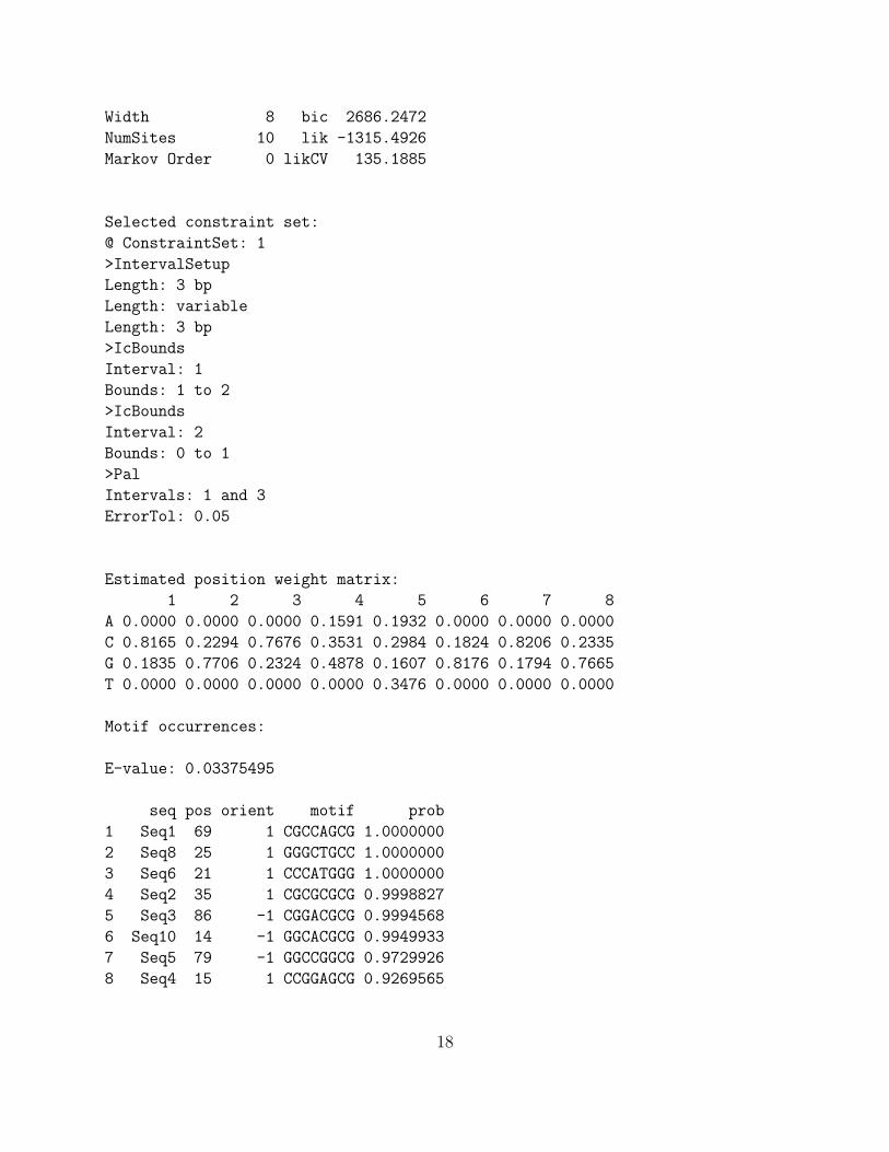
Width 8 bic 2686.2472

NumSites 10 lik -1315.4926

Markov Order 0 likCV 135.1885

Selected constraint set:

@ ConstraintSet: 1

>IntervalSetup

Length: 3 bp

Length: variable

Length: 3 bp

>IcBounds

Interval: 1

Bounds: 1 to 2

>IcBounds

Interval: 2

Bounds: 0 to 1

>Pal

Intervals: 1 and 3

ErrorTol: 0.05

Estimated position weight matrix:

1 2 3 4 5 6 7 8

A 0.0000 0.0000 0.0000 0.1591 0.1932 0.0000 0.0000 0.0000

C 0.8165 0.2294 0.7676 0.3531 0.2984 0.1824 0.8206 0.2335

G 0.1835 0.7706 0.2324 0.4878 0.1607 0.8176 0.1794 0.7665

T 0.0000 0.0000 0.0000 0.0000 0.3476 0.0000 0.0000 0.0000

Motif occurrences:

E-value: 0.03375495

seq pos orient motif prob

1 Seq1 69 1 CGCCAGCG 1.0000000

2 Seq8 25 1 GGGCTGCC 1.0000000

3 Seq6 21 1 CCCATGGG 1.0000000

4 Seq2 35 1 CGCGCGCG 0.9998827

5 Seq3 86 -1 CGGACGCG 0.9994568

6 Seq10 14 -1 GGCACGCG 0.9949933

7 Seq5 79 -1 GGCCGGCG 0.9729926

8 Seq4 15 1 CCGGAGCG 0.9269565

18

9 Seq7 69 -1 CGGGCGGG 0.9082883

10 Seq9 7 1 CGCCCGCG 0.9020536

The cand slot of the cosmo object consists of a data frame that summarizes the modelselection process:

> res@cand

conSet model width wCrit modCrit conCrit

1 1 OOPS 7 2705.698 NA NA

2 1 OOPS 8 2686.247 -1315.493 133.2590

3 1 TCM 7 2720.641 NA NA

4 1 TCM 8 2706.129 -1324.282 NA

5 2 OOPS 7 2731.628 NA NA

6 2 OOPS 8 2729.742 -1337.240 142.9390

7 2 TCM 7 2736.589 -1342.966 NA

8 2 TCM 8 2738.835 NA NA

Note that the E-value criterion was evaluated for all candidate models to select the optimalmotif width for each given combination of model type and constraint. The model typecritertion then needs to be only evaluated for that each combination of model type, constraintset and selected motif width. The constraint set criterion, lastly, needs to be evaluated onlyfor the optimal motif widht and model type for each candidate constraint set. In this case,cosmo selected a motif width of 8, the one-occurrence-per-sequence model, and the firstconstraint set, choices that agree well with the data-generating distribution described above.

The alignment of predicted motif occurrences is stored in the motifs slot of the cosmo

output object:

> summary(res@motifs)

Motif sites:

E-value: 0.03375495

seq pos orient motif prob

1 Seq1 69 1 CGCCAGCG 1.0000000

2 Seq8 25 1 GGGCTGCC 1.0000000

3 Seq6 21 1 CCCATGGG 1.0000000

4 Seq2 35 1 CGCGCGCG 0.9998827

5 Seq3 86 -1 CGGACGCG 0.9994568

6 Seq10 14 -1 GGCACGCG 0.9949933

7 Seq5 79 -1 GGCCGGCG 0.9729926

8 Seq4 15 1 CCGGAGCG 0.9269565

9 Seq7 69 -1 CGGGCGGG 0.9082883

10 Seq9 7 1 CGCCCGCG 0.9020536

19

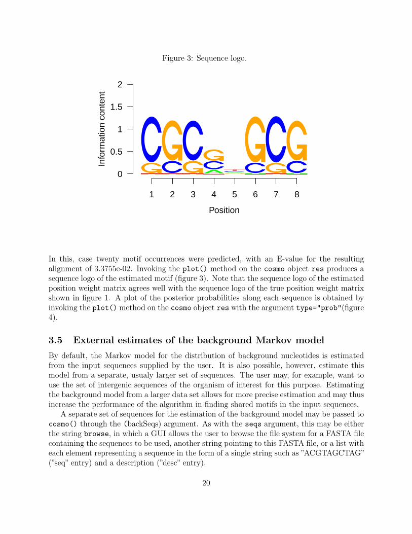
Figure 3: Sequence logo.

1 2 3 4 5 6 7 8

Position

0

0.5

1

1.5

2

Info

rmat

ion

cont

ent

In this, case twenty motif occurrences were predicted, with an E-value for the resultingalignment of 3.3755e-02. Invoking the plot() method on the cosmo object res produces asequence logo of the estimated motif (figure 3). Note that the sequence logo of the estimatedposition weight matrix agrees well with the sequence logo of the true position weight matrixshown in figure 1. A plot of the posterior probabilities along each sequence is obtained byinvoking the plot() method on the cosmo object res with the argument type="prob"(figure4).

3.5 External estimates of the background Markov model

By default, the Markov model for the distribution of background nucleotides is estimatedfrom the input sequences supplied by the user. It is also possible, however, estimate thismodel from a separate, usualy larger set of sequences. The user may, for example, want touse the set of intergenic sequences of the organism of interest for this purpose. Estimatingthe background model from a larger data set allows for more precise estimation and may thusincrease the performance of the algorithm in finding shared motifs in the input sequences.

A separate set of sequences for the estimation of the background model may be passed tocosmo() through the (backSeqs) argument. As with the seqs argument, this may be eitherthe string browse, in which a GUI allows the user to browse the file system for a FASTA filecontaining the sequences to be used, another string pointing to this FASTA file, or a list witheach element representing a sequence in the form of a single string such as ”ACGTAGCTAG”(”seq” entry) and a description (”desc” entry).

20

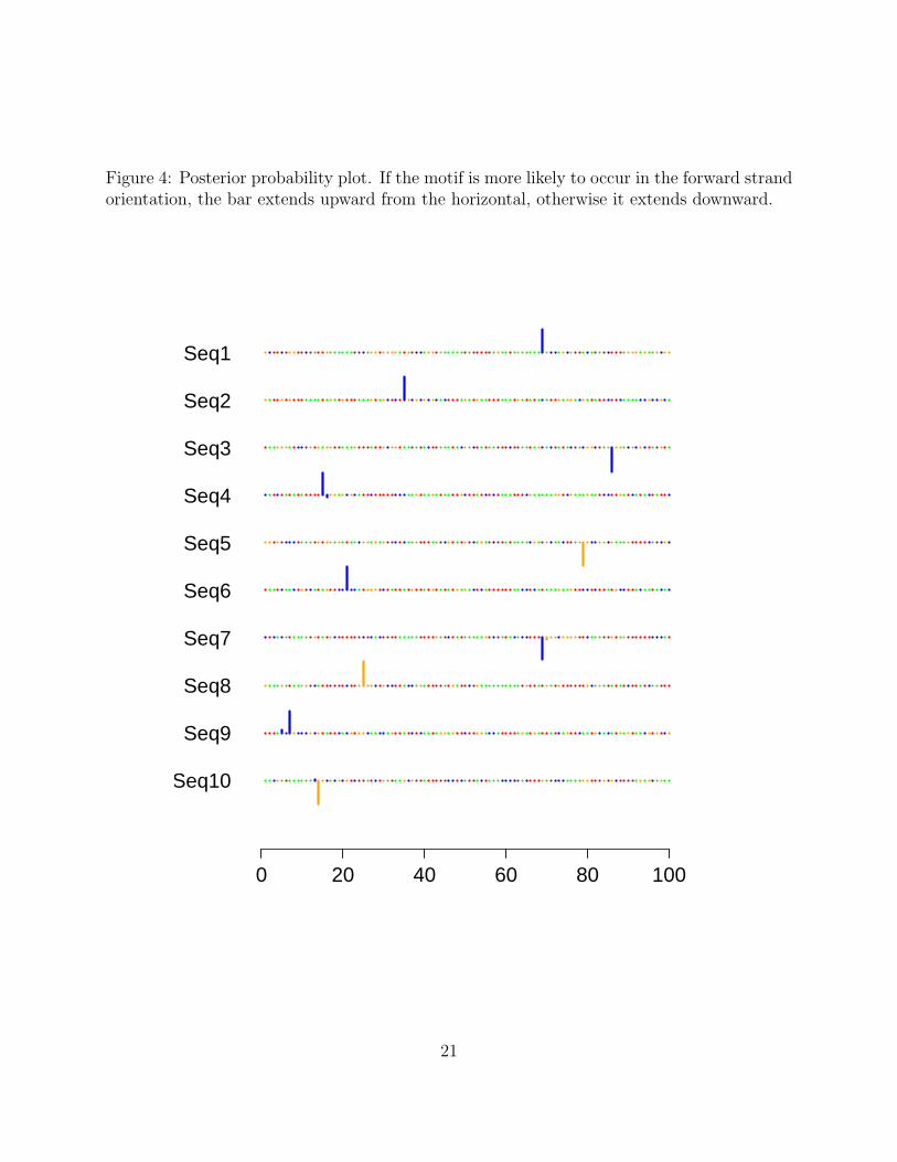
Figure 4: Posterior probability plot. If the motif is more likely to occur in the forward strandorientation, the bar extends upward from the horizontal, otherwise it extends downward.

Seq10

Seq9

Seq8

Seq7

Seq6

Seq5

Seq4

Seq3

Seq2

Seq1

0 20 40 60 80 100

21

If the background data set is large, one may wish to estimate the background Markovmodel in a preliminary step and then pass the obtained estimates to all following calls tocosmo(). The function bgModel() can be used for this purpose:

> args(bgModel)

function (seqs, order = NULL, fold = 5, maxOrder = 6)

NULL

Its main argument consists of the sequences from which the background model is to be esti-mated. If a Markov model of a specific order is desired, this order may be specified throughthe order argument. If order==NULL, the appropriate order is chosen data-adaptivelythrough likelihood-based cross-validation. This approach will larger orders, with correspond-ing models that become more difficult to estimate, as the amount of available data increases.The maxOrder argument gives the largest candidate order that is to be considered. To obtainan estimate of the background Markov model from a set of example sequences contained inthe file bgSeqs, we might use the call

> bgFile <- system.file("Exfiles", "bgSeqs", package = "cosmo")

> tm <- bgModel(bgFile)

cvOrder: Order of background Markov model estimated as order = 2 by CV

The output produced by bgModel() is a list containing the selected order, a summary ofthe Kullback-Leibler divergences for the different candidate orders, as well as the estimatedtransition matrices:

> tm

$transMat

$transMat$order0

A C G T

-- 0.3210294 0.1994118 0.1820588 0.2975

$transMat$order1

A C G T

A 0.3581267 0.1864096 0.1769972 0.2784665

C 0.3621262 0.2045035 0.1513474 0.2820229

G 0.2983023 0.2215036 0.1843169 0.2958771

T 0.2675569 0.1965875 0.2064787 0.3293769

$transMat$order2

A C G T

AA 0.4163449 0.1570142 0.1898327 0.2368082

22

AC 0.3797781 0.1997534 0.1553637 0.2651048

AG 0.3328999 0.2015605 0.1768531 0.2886866

AT 0.3649876 0.1775392 0.1725846 0.2848885

CA 0.3159509 0.2361963 0.1758691 0.2719836

CC 0.4007220 0.2003610 0.1624549 0.2364621

CG 0.2926829 0.2243902 0.1658537 0.3170732

CT 0.2172775 0.2185864 0.2028796 0.3612565

GA 0.3717775 0.1763908 0.1818182 0.2700136

GC 0.3345521 0.2230347 0.1590494 0.2833638

GG 0.3114035 0.2609649 0.1600877 0.2675439

GT 0.2855191 0.1680328 0.2745902 0.2718579

TA 0.3022181 0.1903882 0.1561922 0.3512015

TC 0.3362720 0.1989924 0.1347607 0.3299748

TG 0.2598802 0.2179641 0.2131737 0.3089820

TT 0.1966967 0.2162162 0.2027027 0.3843844

$order

[1] 2

$klDivs

order klDiv

1 0 1.085906e+03

2 1 1.082700e+03

3 2 1.077639e+03

4 3 1.078179e+03

5 4 1.797693e+308

6 5 Inf

7 6 Inf

The transMat element of this list contains one estimated transition matrix for each orderbetween zero and the selected order. The entry in cell (i, j) of a given transition matrix givesthe estimated probability of observing nucleotide j in a given position after having observedthe tuple i in the previous k positions. The Kullback-Leibler divergences summarized in theklDivs element of the output give the estimated risk for each candidate order correspondingto the minus log loss function; likelihood-based cross-validation selects the order with theminimal Kullback-Leibler divergence. The estimated transition matrix may be passed tocosmo() through the transMat argument:

> res <- cosmo(seqs = seqFile, constraints = "None", minW = 8,

+ maxW = 8, models = "OOPS", transMat = tm$transMat)

> res

23

1 2 3 4 5 6 7 8

A 0.0000 0.0000 0.000 0.2700 0.2000 0 0.000 0.0000

C 0.7544 0.1999 0.578 0.3818 0.4513 0 0.778 0.1752

G 0.2456 0.8001 0.422 0.3482 0.1189 1 0.222 0.8248

T 0.0000 0.0000 0.000 0.0000 0.2299 0 0.000 0.0000

MEME allows the user to specify the background Markov model in a slightly different format.The files it accepts for specifyint a 1st-order Markov model, for example, are of the form

# tuple frequency_non_coding

a 0.324

c 0.176

g 0.176

t 0.324

# tuple frequency_non_coding

aa 0.119

ac 0.052

ag 0.056

at 0.097

ca 0.058

cc 0.033

cg 0.028

ct 0.056

ga 0.056

gc 0.035

gg 0.033

gt 0.052

ta 0.091

tc 0.056

tg 0.058

tt 0.119

Such files contain estimates of all relevant tuple frequencies. Note that these frequencies aredifferent from the conditional probabilities given in a transition matrix: The tuple frequenciesgive an estimate of the probability of observing a given tuple, while the frequencies containedin a transition matrix give estimates of the probality of observing a given nucleotide giventhe previous k nucleotides. Thus, the entries in each row of a transition matrix must sumto 1.0, not the entries in an entire matrix, as is the case with a MEME-style tupe frequencymatrix. A MEME-style background file may be passed to cosmo() through the bfile argument.Alternatively, a MEME-style background file may be converted into a transition matrix by usingthe function bfile2tmat():

> tmat <- bfile2tmat(bfile)

> tmat

24

$order0

A C G T

-- 0.324 0.176 0.176 0.324

$order1

A C G T

A 0.3672840 0.1604938 0.1728395 0.2993827

C 0.3314286 0.1885714 0.1600000 0.3200000

G 0.3181818 0.1988636 0.1875000 0.2954545

T 0.2808642 0.1728395 0.1790123 0.3672840

3.6 Software Design

The following features of the programming approach employed in cosmo may be of interestto users.

Class/method object-oriented programming. Like many other Bioconductor pack-ages, cosmo has adopted the S4 class/method objected-oriented programming approach pre-sented in Chambers (1998). In particular, a new class, cosmo, is defined to represent theresults obtained by the constrained motif search algorithm. As discussed to some extentabove, several methods are provided to operate on this class.

Calls to C. The R package was derived from an earlier stand-alone application thatwas written entirely in C. This design was necessary to ensure that the computationallyintensive constrained optimization algorithm does not take too much time. The constrainedoptimiziation itself is carried out using the donlp2() function by Peter Spellucci, availableat http://plato.asu.edu/ftp/donlp2/donlp2_intv_dyn.tar.gz.

3.7 License

The cosmo package incorporates two sources of foreign code whose free use has been restrictedto research purposes. Commercial purposes require permission and licensing by the ownersof the copyright to that code. This is true for the donlp2() function that is used here toperform the constrained optimization of the likelihood function as well as of code that isused by cosmo to compute the E-value criterion. The copyright to donlp2() is owned by itsauthor, Peter Spellucci; the copyright to the second piece of code, written by Timoty Bailey,is owned by the Regents of the University of California. For these reasons, the cosmo packagemust likewise be restricted to research purposes, with commercial uses requiring permissionby Oliver Bembom, Peter Spellucci, as well as the Regents of the University of California.

The license under with donlp2() is distributed furthermore requires that its use must beacknowledged in any publication containing results obtained with donlp2() or parts of it.The same is hence true for publications containing results obtained with cosmo. Citation ofthe author’s name and netlib-source is suitable for this purpose.

25

4 Discussion

The Bioconductor package cosmo implements a constrained motif detection algorithm thatincludes as an important special case the popular motif detection tool MEME, but also allowsthe user to enhance the performance of the algorithm by specifying constraints on the positionweight matrix to the be estimated.

We note that the same algorithm has also been implemented in the form of a web appli-cation, accessible at http://cosmoweb.berkeley.edu, that allows users to submit jobs todesignated web servers, with results posted in HTML as well as XML format on a tempo-rary web page. In this case, constraint definitions are supplied in a text file according to astraightforward standard. In particular, the R function writeConFile() in the cosmo pack-age can be used to convert a constraintSet or constraintGroup object into such a textfile. Lastly, we have also posted the source code of the original stand-alone C implementationof the algorithm on this web site.

References

H. Akaike. Information theory and an extension of the maximum likelihood principle.Academiai Kiado, 1973.

T.L. Bailey and C.P. Elkan. Unsupervised learning of multiple motifs in biolpolymers usingexpectation maximization. Machine Learning, pages 51–80, 1995.

O. Bembom, S. Keles, and M.J. van der Laan. Supervised detection of conserved motifs inDNA sequences with cosmo. Statistical Applications in Genetics and Molecular Biology:Vol. 6 : Iss. 1, Article 8. URL http://www.bepress.com/sagmb/vol6/iss1/art8.

H.J. Bussemaker, H. Li, and E.D. Siggia. Regulatory element detection using correlationwith expression. Nature Genetics, 27:167–171, 2001.

J.M. Chambers Programming with Data: A Guide to the S Language. Springer Verlag, NewYork, 1998.

E. Davidson. Genomic Regulatory Systems. Development and Evolution. Academic Press,San Diego, 2001.

M.B. Eisen. All motifs are not created equal: structural properties of transcription factor -DNA interactions and the inference of sequences specificity. Genome Biology, 6:P7, 2005.

M.B. Eisen, P.T. Spellman, P.O. Brown, and D. Botstein. Cluster analysis and display ofgenome-wide expression patterns. Proceedings of the National Academy of Science, 95:14863–14868, 1998.

J.W. Fickett and W.W. Wasserman. Discovery and modeling of transcriptional regulatoryregions. Current Opinions in Biotechnology, 11:19–24, 2000.

26

C. Lawrence and A. Reilly. An expectation maximization (EM) algorithm for the identifica-tion and characterization of common sites in unaligned biopolymer sequences. Proteins:Structure, Function and Genetics, 7:41–51, 1990.

C.E. Lawrence, S.F. Altschul, M.S. Boguski, J.S. Liu, A.F. Neuwald, and J.C. Wootton. De-tecting subtle sequence signals: a Gibbs sampling strategy for multiple alignment. Science,262:208–214, 1993.

N.M. Luscombe, S.E. Austin, H.M. Berman, and J.M. Thornton. An overview of the struc-tures of protein-DNA complexes. Genome Biology, 1:1–37, 2000.

A.F. Neuwald, J.S. Liu, and C.E. Lawrence. Gibbs motif sampling: detection of bacterialouter membrane repeats. Protein Science, 4:1618–1632, 1995.

J. Powell. SAGE. The serial analysis of gene expression. Methods of Molecular Biology, 99:297–319, 2000.

F.P. Roth, J.D. Hughes, P.W. Estep, and G.M. Church. Finding DNA regulatory motifswithin unaligned noncoding sequences clustered by whole-genome mRNA quantitation.Nature Biotechnology, 16:939–945, 1998.

A. Sandelin and W.W. Wassermann. Constrained binding site diversity within familiesof transcription factors enhances pattern discovery bioinformatics. Journal of MolecularBiology, 338:207–215, 2004.

T. D. Schneider, G. D. Stormo, L. Gold, and A. Ehrenfeucht. Information content of bindingsites on nucleotide sequences. Journal of Molecular Biology, 188:415–431, 1986.

T. D. Schneider, and R. R. Stephens. Sequence Logos: A New Way to Display ConsensusSequences Nucleic Acid Research, 18:6097–6100, 1990.

G. Schwarz. Estimating the dimension of a model. Annals of Statistics, 6:461–464, 1978.

W. Thompson, E.C. Rouchka, and C.E. Lawrence. Gibbs recursive sampler: finding tran-scription factor binding sites. Nucleic Acid Research, 31:3580–3585, 2003.

M.J. van der Laan, S. Dudoit, and S. Keles. Asymptotics optimality of likelihood basedcross-validation. Technical Report 125, Division of Biostatistics, University of California,Berkeley, 2003. URL www.bepress.com/ucbbiostat/paper125.

C.T. Workman and G.D. Stormo. ANN-Spec: a method for discovering transcription fac-tor binding sites with improved specificity. In Proceedings of the Pacific Symposium onBiocomputation, pages 467–478, 2000.

27