Utah State UniversityDigitalCommons@USU

Mathematics and Statistics Faculty Publications Mathematics and Statistics

2009

Superposition Formulas for Darboux IntegrableExterior Differential Sys-temsIan M. AndersonUtah State University

Mark E. FelsUtah State University

Peter J. Vassiliou

Follow this and additional works at: https://digitalcommons.usu.edu/mathsci_facpub

Part of the Mathematics Commons

This Article is brought to you for free and open access by the Mathematicsand Statistics at DigitalCommons@USU. It has been accepted for inclusionin Mathematics and Statistics Faculty Publications by an authorizedadministrator of DigitalCommons@USU. For more information, pleasecontact dylan.burns@usu.edu.

Recommended CitationIan M. Anderson, Mark E. Fels, Peter J. Vassiliou, Superposition formulas for exterior differential systems, Advances in Mathematics,Volume 221, Issue 6, 20 August 2009, Pages 1910-1963, ISSN 0001-8708, 10.1016/j.aim.2009.03.010.

arX

iv:0

708.

0679

v2 [

mat

h.D

G]

11

Jun

2008

Superposition Formulas for

Exterior Differential Systems

Ian Anderson

Dept of Math. and Stat.

Utah State University

Mark Fels

Dept of Math. and Stat.

Utah State University

Peter Vassiliou

Dept. of Math and Stat.

University of Canberra

June 11, 2008

1

Introduction 1

1 Introduction

In this paper we use the method of symmetry reduction for exterior differ-

ential systems to obtain a far-reaching generalization of Vessiot’s integration

method [27], [28] for Darboux integrable, partial differential equations. This

group-theoretic approach provides deep insights into this classical method; un-

covers the fundamental geometric invariants of Darboux integrable systems;

provides for their algorithmic integration; and has applications well beyond

those currently found in the literature. In particular, our integration method

is applicable to systems of hyperbolic PDE such as the Toda lattice equations,

[19], [20], [22], 2-dimensional wave maps [3] and systems of overdetermined PDE

such as those studied by Cartan [8].

Central to our generalization of Vessiot’s work is the novel concept of a

superposition formula for an exterior differential system I on a manifold M .

A superposition formula for I is a pair of differential systems W, W, defined on

manifolds M1 and M2, and a mapping

Σ: M1 ×M2 →M (1.1)

such that

Σ∗(I) ⊂ π∗1(W) + π∗

2(W). (1.2)

Here π∗1(W + π∗

2(W) is the differential system generated by the pullbacks of Wand W to the product manifold M1 ×M2 by the canonical projection maps π1

and π2. It is then clear that if φ : N1 → M1 and φ : N2 → M2 are integral

manifolds for W and W , then

φ = Σ (φ, φ) : N1 ×N2 →M (1.3)

is an (possibly non-immersed) integral manifold of I.

In this article we shall

[i] establish general sufficiency conditions (in terms of geometric invariants of

the differential system I) for the existence of a superposition formula;

[ii] establish general sufficiency conditions under which the superposition for-

mula gives all local integral manifolds of I in terms of the integral manifolds

of π∗1(W)+π∗

2(W) on M1×M2 (in which case we say that the superposition

formula is surjective);

[iii] provide an algorithmic procedure for finding the superposition formula; and

Introduction 2

[iv] demonstrate the effectiveness of our approach with an extensive number of

examples and applications.

Differential systems admitting superposition formula are easily constructed

by symmetry reduction. To briefly describe this construction, let G be a sym-

metry group of a differential system W on a manifold N . We assume that the

quotient space M = N/G of N by the orbits of G has a smooth manifold struc-

ture for which the projection map q : N → M is smooth. We then define the

G reduction of W or quotient of W by G as the differential system on M

given by

W/G = ω ∈ Ω∗(M) |q∗(ω) ∈ W . (1.4)

The traditional application of symmetry reduction has been to integrate W by

integrating W/G. See, for example, [1].

But now suppose that differential systems W and W on manifolds M1 and

M2 have a common symmetry group G. Define the differential system W =

π∗1(W)+ π∗

2(W) on M1 ×M2 and let G act on M1 ×M2 by the diagonal action.

Then, by definition, the quotient map q : M1 × M2 → M = (M1 × M2)/G

defines a superposition formula for the quotient differential system W/G on M .

In this paper we discover the means by which the inverse process to symmetry

reduction is possible, that is, we show how certain general classes of differential

systems I on M can be identified with a quotient system W/G in which case

the integral manifolds of I can then be found from those of W and W.

To intrinsically describe the class of differential systems for which we shall

construct superposition formulas, we first introduce the definition of a decom-

posable differential system.

Definition 1.1. An exterior differential system I on M is decomposable of

type [p, q], where p, q ≥ 2, if about each point x ∈M there is a coframe

θ1, . . . , θr, σ1, . . . , σp, σ1, . . . , σq, (1.5)

such that I is algebraically generated by 1-forms and 2-forms

I = θ1, . . . , θr, Ω1, . . . , Ωs, Ω1, . . . , Ωt , (1.6)

where s, t ≥ 1, Ωa ∈ Ω2(σ1, . . . , σp), and Ωα ∈ Ω2(σ1, . . . , σq). The differential

systems algebraically generated by

V = θi, σa, Ωα and V = θi, σα, Ωa (1.7)

Introduction 3

are called the associated singular differential systems for I with respect to

the decomposition (1.6).

With the goal of constructing superposition formulas, we have found it most

natural to focus on the case where I is decomposable (but not necessarily Pfaf-

fian) and V and V are (constant rank) Pfaffian1. All of the examples we consider

are of this type. Note that any class r hyperbolic differential system, as defined

in [6], is a decomposable differential system and that the associated character-

istic Pfaffian systems coincide, for r > 0, with the singular systems(1.7).

The definition of a Darboux integrable, decomposable differential system is

given in terms of its singular systems. For any Pfaffian system V , let V (∞)

denoted the largest integrable subbundle of V . The rank of V (∞) gives the

number of functionally independent first integrals for V . By definition, a scalar

second order partial differential equation in the plane is Darboux integrable if

the associated singular Pfaffian systems V and V each admit at least 2 (func-

tionally independent) first integrals. Thus, in order to generalize the definition

of Darboux integrablity, we must determine the required number of function-

ally independent first integrals necessary to integrate a general decomposable

Pfaffian system. We do this with the following definitions.

Definition 1.2. A pair of Pfaffian systems V and V define a Darboux pair

if the following conditions hold.

[i] V + V(∞)

= T ∗M and V + V(∞)

= T ∗M. (1.8)

[ii] V(∞) ∩ V∞

= 0 . (1.9)

[iii] dω ∈ Ω2(V ) + Ω2(V ) for all ω ∈ Ω1(V ∩ V ) . (1.10)

Definition 1.3. Let I be a decomposable differential system and assume that

the associated singular systems V and V are Pfaffian. Then I is said to be

Darboux integrable if V , V define a Darboux pair.

Property [i] of Definition 1.2 is the critical one – it will insure that there

are a sufficient number of first integrals to construct a superposition formula.

Property [ii] is a technical condition which states simply that V and V share no

1We use the term Pfaffian system to designate either a constant rank subbundle V of T ∗M

or the differential system, denoted by the corresponding calligraphic letter V , generated by

the sections of V .

Introduction 4

common integrals – this condition can always be satisfied by restricting V and

V to a level set of any common integrals. The form of the structure equations

for V ∩ V required by property [iii] is always satisfied when V and V are the

singular Pfaffian systems for a decomposable differential system I.

Our main result can now be stated.

Theorem 1.4. Let I be a decomposable differential system on M whose asso-

ciated singular Pfaffian systems V , V define a Darboux pair. Then there are

Pfaffian systems W1 and W2 on manifolds M1 and M2 which admit a common

Lie group G of symmetries and such that

[i] the manifold M can be identified (at least locally) as the quotient of M1×M2

by the diagonal action of the group G;

[ii] I = (π∗1(W + π∗

2(W))/G; and (1.11)

[iii] the quotient map q : M1 ×M2 → M defines a surjective superposition for-

mula for I.

The manifolds M1 and M2 in Theorem 1.4 are simply any maximal integral

manifolds for V(∞)

and V(∞)

and the Pfaffian systems W1 and W2 are just the

restrictions of V and V to these manifolds. But the proper identification of the

Lie group G and its action on M1 and M2 is not so easy to uncover. This is done

through a sequence of non-trivial coframe adaptations and represents the prin-

ciple technical achievement of the paper (See Theorem 4.1 and Definition 5.7)

We call G the Vessiot group for the Darboux integrable, differential system

I.

The paper is organized as follows. In Section 2 we obtain some simple

sufficiency conditions for a differential system to be decomposable and we give

necessary and sufficient conditions for a Pfaffian system to be decomposable

(Theorem 2.3). We also introduce the initial adapted coframes for a Darboux

pair (Theorem 2.9). In Section 3 we answer the question of when the symmetry

reduction of a Darboux pair is also a Darboux pair (Theorem 3.2) and we

use this result to give a general method for constructing Darboux integrable

differential systems (Theorem 3.3). Section 4 establishes the sequence of coframe

adaptations leading to the definition of the Vessiot group G and its action on

M and hence on M1 and M2 (Theorem 4.1). In Section 5 we construct the

superposition formula (Theorem 5.10) and prove that it may be identified with

Introduction 5

the quotient for the diagonal action of the Vessiot group. This proves Theorem

1.4.

A substantial portion of the paper is devoted to examples. These exam-

ples, given in Section 6, provide closed-form general solutions to a wide range

of differential equations, explicitly illustrate the various coframe adaptations

of Section 4, and underscore the importance of the Vessiot group as the fun-

damental invariant for Darboux integrable differential systems. The first two

examples are taken from the classical literature. The equation considered in

Example 6.1 is specifically chosen to illustrate in complete detail all the various

coframe adaptations used to determine the superposition formula. In Example

6.2 we integrate all non-linear Darboux equations of the type uxx = f(uyy) (with

second order invariants) and relate the integration of these equations to Car-

tan’s classification of rank 3 Pfaffian systems in 5 variables [7]. This connection

between the method of Darboux and Cartan’s classification is apparent from

our interpretation of the method of Darboux in terms of symmetry reduction of

differential systems.

In Examples 6.3 and 6.4 we present a number of examples of Darboux in-

tegrable equations where the unknown function takes values in a group or in a

non-commutative algebra. Example 6.3 provides us with a system whose Vessiot

group is an arbitrary Lie group G.

Some of the simplest examples of systems of Darboux integrable partial dif-

ferential equations can be constructed by the coupling of a nonlinear Darboux

integrable scalar equation to a linear or Moutard-type equation. These are pre-

sented in Example 6.5. It is noteworthy that for these equations the Vessiot

group is a semi-direct product of the Vessiot group for the non-linear equa-

tion with an Abelian group. The representation theoretical implications of this

observation will be further explored elsewhere.

In Example 6.6 we illustrate the computational power of our methods by

explicitly integrating the B2 Toda lattice system. While the general solution

to the An Toda systems were known to Darboux, this is, to the best of our

knowledge, the first time explicit general solutions to other Toda systems have

been given. Based on this work we conjecture that the Vessiot group for the g

Toda lattice system, where g is any semi-simple Lie group, is the associated Lie

group G itself. In Example 6.7 we integrate a wave map system – this system

admits a number of interesting geometric properties which will be explored

Introduction 6

in detail in a subsequent paper. Finally, in Example 6.8, we present some

original examples of Darboux integrable, non-linear, over-determined systems

in 3 independent variables.

The extensive computations required by all these examples were done using

the DifferentialGeometry package in Maple 11. This research was supported by

NSF grant DMS-0410373 and DMS-0713830.

Preliminaries 7

2 Preliminaries

2.1 Decomposable Differential Systems

In this section we give some simple necessary conditions, in terms of the

notion of singular vectors, for a differential system2 I to be decomposable (see

Definition 1.1); we give sufficient conditions for a Pfaffian system to be decom-

posable; and we address the problem (see Theorem 2.6) of re-constructing a

decomposable differential system from its associated singular systems.

Let I be a differential system on M . Fix a point x in M and let

E1x(I) = X ∈ TxM | θ(X) = 0 for all 1-forms θ ∈ I .

The polar equations determined by a non-zero vector X ∈ E1x(I) are, by

definition, the linear system of equations for Y ∈ E1x(I) given by

θ(X,Y ) = 0 for all 2-forms θ ∈ I.

Then X ∈ E1x(I) is said to be regular if the rank of its polar equations is

maximal and singular otherwise.

Lemma 2.1. Let I be a decomposable differential system of type [p, q]. Then

E1x(I) decomposes into a direct sum of p and q dimensional subspaces

E1x(I) = S1 ⊕ S2 (2.1)

such that

[i] every vector in S1 and every vector in S2 is singular; and

[ii] every 2 plane spanned by any pair of vectors X ∈ S1 and Y ∈ S2 is an

integral 2-plane for I.

Proof. Let ∂θi, ∂σa , ∂σα denote the dual frame to (1.5). Then E1x(I) =

span ∂σa , ∂σα and the polar equations for X = X1 +X2, where X1 = ta∂σa

and X2 = sα∂σα , are

Ωa(X1, Y ) = 0 and Ωα(X2, Y ) = 0.

Then, clearly, the vectors X1 and X2 are singular vectors and, moreover, the

plane spanned by X1, X2 is an integral 2-plane.

2We assume that all exterior differential systems are of constant rank.

2.1 Decomposable Differential Systems 8

Remark 2.2. The differential system V defined by (1.7) is the smallest differ-

ential system containing I and Ann(S2) and it is for this reason that we have

opted to called V (and V) the singular differential systems associated to the

decomposition of I.

The necessary conditions for decomposability given in Lemma 2.1 are seldom

sufficient. However, if I is a Pfaffian system and properties [i] and [ii] of Lemma

2.1 are satisfied, then there exists a local coframe

θ1, . . . , θr, σ1, . . . , σp, σ1, . . . , σq

on M with I = θi and with structure equations

dθi ≡ Aiab σ

a ∧ σb +Biαβ σ

α ∧ σβ mod I. (2.2)

At each point x0 of M define linear maps

A = [Aiab(x0)] : Rr → Λ2(Rp) and B = [Bi

αβ(x0)] : Rr → Λ2(Rq). (2.3)

Theorem 2.3. Let I be a Pfaffian system. Then I is decomposable if properties

[i] and [ii] of Lemma 2.1 are satisfied; the matrices Aiab and Bi

αβ given by (2.2),

are non-zero, constant rank; and

dim(

ker(A) + ker(B))

= rank I. (2.4)

Proof. Equation (2.4) implies that we can find r linearly independent r dimen-

sional column vectors T 1,. . . , T r1,. . . , T r2, . . . , T r such that

ker(A) ∩ ker(B) = spanT 1, . . . , T r1 ,ker(B) = spanT 1, . . . , T r1, T r1+1, . . . , T r2 , and

ker(A) = spanT 1, . . . , T r1 , T r2+1, . . . , T r .

The 1-forms θi = tij θj , where T i = [tij ], then satisfy

dθi ≡ 0 for i = 1 . . . r1,

dθi ≡ tijAjab σ

a ∧ σb for i = r1 + 1 . . . r2,

dθi ≡ tijBjαβ σ

α ∧ σβ for i = r2 + 1 . . . r,

(2.5)

and the decomposability of I follows by taking Ωi = tijAjab σ

a ∧ σb for i =

r1 + 1 . . . r2 and Ωi = tijBjαβ σ

a ∧ σb for i = r2 + 1 . . . r. That the integers s and

t in Definition 1.1 satisfy s, t ≥ 1 follows from the fact that Aiab and Bi

αβ are

non-zero and that [tij ] is invertible.

2.1 Decomposable Differential Systems 9

Corollary 2.4. If I is a decomposable Pfaffian system, then the singular sys-

tems V and V are also Pfaffian.

Proof. This is immediate from (1.7) and (2.5).

To each decomposable exterior differential system I we have associated a

pair of differential systems V and V and, when these are Pfaffian, we have

defined what it means for V , V to define a Darboux pair. In our subsequent

analysis, the Darboux pair V , V will be taken as the fundamental object of

study. From this viewpoint, it becomes important to address the problem of

reconstructing the EDS I from its singular systems. To this end, we introduce

the following novel construction.

Definition 2.5. Let V and V be two differential systems on a manifold M .

Define a new differential system K = V ∩+ V to be the exterior differential system

whose integral elements are precisely the integral elements of V, the integral

elements of V, and the sum of integral elements of V with integral elements of

V.

This definition is motivated by two observations. First we note that if I is a

decomposable exterior differential system with singular Pfaffian systems V and

V then in general I properly contains the Pfaffian system with generators V ∩ Vand is properly contained in the EDS V ∩V so that neither of these set-theoretic

constructions reproduce I.

Secondly, one can interprete the EDS K in Definition 2.5 as satisfying an

infinitesimal superposition principle with respect to V, V at the level

of integral elements. Of course, this by itself does not imply that K admits a

superposition principle for its integral manifolds. The main results of this article

can then be re-formulated as follows: if the EDS K admits a superposition

principle for its integral elements with respect to a Darboux pair V , V , then

K admits a superposition principle for its integral manifolds.

Theorem 2.6. If I is a decomposable exterior differential system with singular

differential systems V and V, then I = V ∩+ V.

Proof. We first remark that the differential system V ∩+ V is always contained in

V ∩ V . Let θi, σa, σα be the coframe given by Definition 1.1. By definition,

the algebraic generators for V and V are

V = θi, σa, Ωβ and V = θ, σα, Ωb

2.2 The first adapted coframes for a Darboux pair 10

from which it is not difficult to show that

V ∩ V = θi, Ωb, Ωβ , σa ∧ σα.

Since ∂σα defines a 1-integral element for V and ∂σα defines a 1-integral element

for V , the 2-plane spanned by ∂σα , ∂σa must be a integral element for V ∩+ Vand therefore the forms σa ∧ σα /∈ V ∩+ V . In view of (1.6), we conclude that

V ∩+ V ⊂ I.

To complete the proof, it suffices to check that every (r + s)-form ω ∈ Ivanishes on every plane Er + Es, where Er is an r-integral plane of V and Es

is an s-integral plane of V . The form ω is a linear combination of the wedge

product of the 1-forms in (1.6) with arbitrary (r+ s− 1)-forms ρ and the wedge

product of the 2-forms in (1.6) with arbitrary (r + s − 2)-forms τ . It is clear

that (θi ∧ ρ)|(Er+Es) = 0. The values of (Ωb ∧ τ)|(Er+Es)can be calculated as

linear combinations of terms involving

Ωb(X, Y ), Ωb(X, Y ), Ωb(X, Y ), Ωb(X, Y ),

where X, Y ∈ Er and X, Y ∈ Es. These terms all vanish and in this way we

may complete the proof of the theorem.

2.2 The first adapted coframes for a Darboux pair

Let V , V be a Darboux pair on a manifold M . In addition to the prop-

erties listed in Definition 1.2, we shall assume that the derived systems V(∞)

and V(∞)

, as well as the intersections V(∞) ∩ V , V ∩ V (∞)

and V ∩ V are all

(constant rank) subbundles of T ∗M .

To define our initial adapted coframe for the Darboux pair V , V , we first

chose tuples of independent 1-forms η and η which satisfy

V(∞) ∩ V = spanη and V ∩ V (∞)

= spanη. (2.6a)

Property (1.9) implies that the forms η, η are linearly independent. Then

chose tuples of 1-forms θ, σ and σ such that

V(∞)

= span σ, η , V (∞)= span σ, η , V ∩ V = span θ, η, η (2.6b)

and such that the sets of 1-forms σ, η , σ, η and θ, η, η are linearly

independent.

2.2 The first adapted coframes for a Darboux pair 11

Lemma 2.7. Let V , V be a Darboux pair on a manifold M . Then the 1-

forms θ, σ, η, σ, η satisfying (2.6) define a local coframe for T ∗M and

V = span θ, σ, η, η and V = span θ, η, σ, η . (2.6c)

Proof. From the definitions (2.6a) and (2.6b) it is clear that span θ, σ, η, η ⊂V and span θ, η, σ, η ⊂ V . Property (1.8) then implies that the forms

θ, σ, η, σ, η span T ∗M .

To prove the first of (2.6c), let ω = aθ + b σ + c η + d σ + e η. If ω ∈ V ,

then the 1-forms d σ ∈ V and therefore, by (2.6b), d σ ∈ V ∩ V (∞). Since the

forms η and σ are independent, we must have d = 0 and (2.6c) is established.

To prove the independence of the forms θ, σ, η, σ, η , set ω = 0. Then

the argument just given implies that d = 0 so that bσ ∈ V ∩ V . Therefore

bσ ∈ V(∞)∩ V and this forces b = 0. The independence of the forms θ, η, η

then gives a = c = e = 0 and the lemma is proved.

Any local coframe θ, σ, η, σ, η satisfying (2.6) is called a 0-adapted

coframe for the Darboux pair V , V .We shall also need the definition of a 0-adapted frame as the dual of the

0-adapted coframe. Let

H = ann V , H = ann V , H(∞)

= ann V(∞)

, H(∞)

= ann V(∞)

,

and K = H(∞) ∩ H(∞)

.

(2.7)

The definition of Darboux integrability can be re-formulated in terms of the

distributions H, H ([26]). If we introduce the dual basis ∂θ, ∂σ, ∂η, ∂σ, ∂η to the 0-adapted coframe θ, σ, η, σ, η, that is,

θ(∂θ) = 1, σ(∂σ) = 1, η(∂η) = 1, σ(∂σ) = 1, η(∂η) = 1, (2.8)

with all others pairings yielding 0, then it readily follows that

H = span∂σ , H(∞)

= span∂θ, ∂σ , ∂η ,H = span∂σ, H

(∞)= span∂θ, ∂σ , ∂η ,

and K = span∂θ .

(2.9)

Any local frame ∂θ, ∂σ, ∂η, ∂σ , ∂η satisfying (2.9) is called a 0-adapted

frame.

We shall use the following lemma repeatedly.

2.2 The first adapted coframes for a Darboux pair 12

Lemma 2.8. Let f be a real-valued function on M . If X(f) = 0 for all vector

fields in H, then df ∈ V(∞)

. Likewise, if X(f) = 0 for all vector fields in H,

then df ∈ V(∞)

.

Proof. It suffices to note that if X(f) = 0 for all vector fields X ∈ H , then

Z(f) = Z df = 0 for all vector fields Z ∈ H(∞)

and therefore df ∈ ann H(∞)

=

V(∞)

.

Real-valued functions on M with df ∈ V (or V (∞)) are called first integrals

for V . We denote the algebra of all first integrals for V by Int(V ).

Our 1-adapted coframe for a Darboux pair is easily constructed from com-

plete sets of functionally independent first integrals for V(∞)

and V(∞)

, that is,

locally defined functions I and I such that

V(∞)

= span d I and V(∞)

= span d I .

Complete the 1-forms η in (2.6a) to the local basis (2.6b) for V(∞)

using

forms

σ = d I1 (2.10)

chosen from the d I . Next let I2 be a complementary set of invariants to

the set I1 , that is, I = I1, I2 . Because the forms η belong to V∞

we

can write

η = R0 d I1 + S0 d I2.

Since the 1-forms η are independent of the 1-forms σ, the coefficient matrix S0

must be invertible and we can therefore adjust our local basis of 1-forms η for V

(∞) ∩ V by setting

η = d I2 + R d I1 = d I2 + R σ. (2.11)

The exterior derivatives of these forms are

d η = dR ∧ σ = ∂σ(R) σ ∧ σ + · · ·

and therefore, on account of (1.10), the fact that η ∈ V(∞) ∩ V , and (2.6c), we

must have ∂σ(R) = 0. Lemma 2.8 implies that d(R) ∈ V(∞)

and consequently

d η = E η ∧ σ + F σ ∧ σ. (2.12)

Similar arguments are used to modify the forms σ and η. These adaptations

are summarized in the following theorem.

2.2 The first adapted coframes for a Darboux pair 13

Theorem 2.9. Let V , V be a Darboux pair on a manifold M . Then about

each point of M there exists a 0-adapted coframe θ, σ, η, σ, η with structure

equations

d σ = 0, d η = E η ∧ σ + F σ ∧ σ,

d σ = 0, d η = E η ∧ σ + F σ ∧ σ,(2.13)

dθ ≡ A σ ∧ σ + B σ ∧ σ mod θ, η, η. (2.14)

We remark that the structure equations for the 1-forms θ ∈ V ∩V are a conse-

quence of (1.10) and the properties (2.6) of a 0-adapted coframe. A 1-adapted

coframe for the Darboux pair V , V is a 0-adapted coframe θ, σ, η, σ, η satisfying the structure equations (2.13) and (2.14).

Corollary 2.10. If V , V define a Darboux pair, then V ∩+ V is always a de-

composable exterior differential system for which V and V are singular Pfaffian

systems.

Proof. It follows from Theorem 2.9 that the algebraic generators for V and Vare

V = θ, η, η, σ, F σ ∧ σ, B σ ∧ σ and

V = θ, η, η, σ, F σ ∧ σ, A σ ∧ σ .

From these equations it is not difficult to argue that the differential system V ∩Vhas generators

V ∩ V = θ, η, η, σ ∧ σ, F σ ∧ σ, A σ ∧ σ, F σ ∧ σ, B σ ∧ σ .

A repetition of the arguments used in the proof of Theorem 2.6 shows that

V ∩+ V = θ, η, η, F σ ∧ σ, A σ ∧ σ, F σ ∧ σ, B σ ∧ σ . (2.15)

It is then clear that V ∩+ V is a decomposable differential system (Definition 1.1)

and that V and V are singular Pfaffian systems.

Example 2.11. There are many examples of differential equations which can

be described either by Pfaffian differential systems or by differential systems

generated by 1-forms and 2-forms. Our definition of Darboux integrability in

terms of decomposable differential system is such that theseequations will be

2.2 The first adapted coframes for a Darboux pair 14

Darboux integrable irrespective of their formulation as an exterior differential

system. The simplest example, but by no means the only example, is the wave

equation uxy = 0. The wave equation can be encoded as adifferential system on

manifold of dimensions 5, 6 and 7 by

I1 = θ, dp ∧ dx, dq ∧ dy , V 1 = θ, dp, dx , V = θ, dq, dy ,I2 = θ, θx, dq ∧ dy , V 2 = θ, θx, dp, dx , V 2 = θ, θx, dq, dy ,I3 = θ, θx, θy , V 3 = θ, θx, θy, dp, dx , V 3 = θ, θx, θy, dq, dy ,

where θ = du − p dx − q dy, θx = dp − r dx and θy = dq − t dy. Each of these

satisfy the definition of a decomposable, Darboux integrable differential system.

Consistent with Corollary 2.6, one easily checks that Ii = Vi ∩+ V i.

We remark that for the standard contact system on J1(R,R), that is,

I4 = θ, dp ∧ dx + dq ∧ dy , the Pfaffian systems V 4 = θ, dp, dx and V =

θ, dq, dy , are singular systems which form a Darboux pair but V 4 ∩+ V 4 6= I4.

Equality fails because I4 is not decomposable.

Remark 2.12. In very special cases, such as Liouville’s equation uxy = eu,

one finds that V ∩ V(∞)

= V(∞) ∩ V = 0 so that the vector space sums

appearing in (1.8) are direct sum decompositions. Under these circumstances,

our 0-adapted coframe is simply θ, σ, σ . This initial coframe is then auto-

matically 2-adapted (see Theorem 4.3) and the sequence of coframe adaptations

needed to prove Theorem 4.1 can begin with the third coframe adaptation (Sec-

tion 4.2).

Remark 2.13. We define an involution of a Darboux pair V , V on M

to be a diffeomorphism Φ: M → M such that Φ2 = idM and Φ∗(V ) = V . For

such maps Φ∗(V(∞)

) = V(∞)

and therefore, given 1 adapted co-frame elements

η and σ, one may take

η = Φ∗(η) and σ = Φ∗(σ).

Such involutions are quite common, especially for differential equations arising

in geometric and physical applications, where the diffeomorphism Φ arises from

a symmetry of the differential equations in the independent variables.

The group theoretic construction of Darboux pairs 15

3 The group theoretic construction of Darboux

pairs

3.1 Direct Sums of Pfaffian Systems and Trivial Darboux

Pairs

Let W1 and W2 be differential systems on manifolds M1 and M2. Then the

direct sum W1+W2 is the EDS on M1×M2 generated by the pullbacks of W1

and W2 by the canonical projection maps πi : M1 ×M2 → Mi. The following

theorem shows that if W1 and W2 are Pfaffian, then W1 + W2 is Darboux

integrable in the sense of Definition 1.3.

Theorem 3.1. Let W1 and W2 be Pfaffian systems on manifolds M1 and M2

such that W(∞)1 = W

(∞)2 = 0. Then the direct sum J = W1 +W2 on M1 ×M2

is a decomposable Pfaffian system. The associated singular Pfaffian systems

W = W1 ⊕ Λ1(M2) and W = Λ1(M1) ⊕W2 (3.1)

form a Darboux pair and

W1 + W2 = W ∩+ W , (3.2)

where W1,W2, W, W are the differential systems generated by W1,W2, W , W .

Proof. It is easy to check that J is decomposable with singular systems (3.1).

Properties [i] and [ii] of Definition 1.2 follow directly from (3.1) and the simple

observations that

W(∞)

= Λ1(M2) and W(∞)

= Λ1(M1). (3.3)

Let ω =∑

i(fi θi1 + gi θ

i2), where the coefficients fi, gi ∈ C∞(M1 ×M2) and

the θiℓ ∈ Wℓ are 1-forms in J . Then to check property [iii], it suffices to note

that every summand in the exterior derivative

dω =∑

i

d1fi ∧ θi1 + d2fi ∧ θi

1 + fi d1θi1 + d1gj ∧ θj

2 + d2gj ∧ θj2 + gi d2θ

i2,

where di = dMi, lies either in Ω2(W ) or Ω2(W ). Equation (3.2) is a direct

consequence of Theorem 2.6.

Darboux pairs of the form (3.1) are said to be trivial.

3.2 Symmetry Reduction of Darboux Pairs 16

3.2 Symmetry Reduction of Darboux Pairs

A Lie group G is a regular symmetry group of a differential system

I on a manifold M if there is a regular action of G on M which preserves I. By

the definition of regularity, the quotient space M/G of M by the orbits of G has

a smooth manifold structure such that [i] the projection map q : M → M/G is

a smooth submersion, and [ii] local, smooth cross-sections to q exist on some

open neighborhood of each point of M/G. The G reduction of I or the

quotient of I by G is the differential system on M = M/G given by

I/G = ω ∈ Ω∗(M) |q∗(ω) ∈ I . (3.4)

Details of this construction and basis facts regarding the G reduction of differ-

ential systems are given in [1].

To obtain the main results of this section, we shall require that G be trans-

verse to I in the sense which we now define. Let I be any G invariant sub-

bundle of T ∗M and let Γ be the infinitesimal generators for G. We say that G

is transverse to I if for each x ∈M

Γx ∩ ann Ix = 0 . (3.5)

We say that G is transverse to the differential system I if G is transverse to the

sub-bundle of T ∗M whose sections are 1-forms in I. With this transversality

condition, I/G is assured to be a constant rank differential system whose local

sections can be determined as follows. If A is any sub-bundle of Λk(M) or sub-

algebra of Λ∗(M), then the sub-bundle or sub-algebra of semi-basic forms in

A is defined as

Asb = ω ∈ A |X ω = 0 for all X ∈ Γ . (3.6)

Denote by Isb the sections of I which are semi-basic, that is, which take values

in Λ∗sb

(M). Then one can show (see Lemma 4.1 of [1]) that

(I/G)|U = ξ∗(Isb|U ), (3.7)

where U is any (sufficiently small) open set of M , ξ : U → M is a smooth

cross-section of q, and U = q−1(U). We remark that the G reduction I/G of a

Pfaffian system I need not be Pfaffian (but see [c] below).

For the proof of the next theorem on the G reduction of Darboux pairs, we

shall require the following elementary facts regarding the reduction of Pfaffian

3.2 Symmetry Reduction of Darboux Pairs 17

systems. Here I and J are Pfaffian systems with regular symmetry group G, we

assume that G is transverse to I, and the G bundle reduction of I is defined as

I/G = ω ∈ Λ1(M) |q∗(ω) ∈ I . (3.8)

By transversality, this is a sub-bundle of T ∗M of dimension dim I − q, where q

is the dimension of the orbits of G.

[a] If I ⊂ J , then G is transverse to J .

[b] If G is transverse to I ∩ J , then (I/G) ∩ (J/G) = (I ∩ J)/G.

[c] If G is transverse to the derived system I ′, then the quotient differen-

tial system I/G is the constant rank Pfaffian system determined by I/G and

(I/G)′ = I ′/G .

[d] If G is transverse to I(∞), then (I/G)(∞) = I(∞)/G.

Facts [a] and [b] are trivial, while [c] is Theorem 5.1 in [1]. Fact [d] follows

from [a] and [c] by induction.

Finally, we shall also use the following technical observation. If Z is a sub-

bundle of I, then the canonical pairing (X,ω) = ω(X) on Γx×Zx, where x ∈M ,

is non-degenerate if and only if

I = q∗(I/G) ⊕ Z. (3.9)

Such bundles Z can always be constructed locally on G invariant open subsets

of M .

Theorem 3.2. Let W , W be a Darboux pair on M . Suppose that G is a

regular symmetry group of W and W and that, in addition, G is transverse to

W∩W (∞)and W

(∞)∩W . Then the quotient differential systems W/G, W/G on M are (constant rank) Pfaffian systems and form a Darboux pair.

Proof of Theorem 3.2. Since W(∞)∩W ⊂ W

(∞) ⊂ W′ ⊂ W and G is transverse

to W(∞) ∩ W , it follows that G is transverse to W

(∞), W

′and W . Thus, by

[c], V = W/G and, similarly, V = W/G are the Pfaffian systems for V = W/G

and V = W/G. By [d]

(W/G)(∞) = W(∞)

/G and (W/G)(∞) = W(∞)

/G. (3.10)

3.2 Symmetry Reduction of Darboux Pairs 18

We now verify the three conditions in Definition 1.2 for V , V to be a

Darboux pair. From (3.8), (3.10) and fact [b] we deduce that

dim(V ) = dim W − q,

dim(V(∞)

) = dim(W(∞)

/G) = dim W(∞) − q, and

dim(V ∩ V (∞)) = dim

(

(W/G) ∩ (W(∞)

/G))

= dim(

(W ∩ W (∞))/G

)

= dim(W ∩ W (∞)) − q.

From these equations and property [i] in the definition of Darboux pair (applied

to W , W ) we calculate

dim(

V + V(∞))

= dim(V ) + dim(V(∞)

) − dim(V ∩ V (∞))

= dim W + dim W(∞)

+ dim(W ∩ W (∞)) − q

= dimM − q = dimM.

This proves that V + V(∞)

= T ∗M . Similar arguments yield V(∞)

+ V = T ∗M

and so V , V satisfy property [i] of a Darboux pair.

To check that V , V satisfy property [ii] of a Darboux pair, we use [b] and

(3.10) to calculate

V(∞) ∩ V (∞)

= (W(∞)

/G) ∩ (W(∞)

/G) = (W(∞) ∩ W (∞)

)/G = 0. (3.11)

To prove property [iii] of a Darboux pair, we first prove that

[Λ2(W ) + Λ2(W )]sb = Λ2(W sb) + Λ2(W sb). (3.12)

It suffices to check this locally. Since G acts transversally to W(∞) ∩ W , there

is a locally defined sub-bundle Z of W(∞) ∩ W such that the canonical pairing

on Γ×Z is pointwise non-degenerate. For any such sub-bundle Z we have that

W = W sb ⊕ Z and W = W sb ⊕ Z and therefore

Λ2(W ) + Λ2(W ) = Λ2(W sb) + Λ2(W sb) + T ∗M ∧ Z.

This (local) decomposition immediately leads to (3.12). To complete the proof of

property [iii], let ω ∈ V ∩ V . Then q∗(ω) ∈ W ∩W and hence, by the properties

of the Darboux pair W , W and (3.12), q∗(dω) ∈ Ω2(W sb) + Ω2(W sb). We

pullback this last equation by a local cross-section of q and invoke (3.7) to

conclude that dω ∈ Ω2(V ) + Ω2(V ).

3.2 Symmetry Reduction of Darboux Pairs 19

Theorem 3.3. Let W , W be a Darboux pair on M . Suppose that G is a

regular symmetry group of W and W and that, in addition, G is transverse to

W(∞) ∩ W and W ∩ W (∞)

. Then

(W ∩+ W)/G = (W/G) ∩+ (W/G). (3.13)

Proof. We first remark that Theorem 3.2 implies that V = W/G and V = W/G

define a Darboux pair and, second, that it suffices to check (3.13) locally.

Transversality implies that there are locally defined sub-bundles Z ⊂ W(∞)∩

W and Z ⊂ W ∩ W (∞)on which the natural pairing with Γ (the infinitesimal

generators for G) is non-degenerate at each point x ∈ M . It follows from (3.9)

that

W(∞) ∩ W = q∗(V

(∞) ∩ V ) ⊕ Z, W(∞)

= q∗(V(∞)

) ⊕ Z, (3.14a)

W ∩ W (∞)= q∗(V ∩ V (∞)

) ⊕ Z, W(∞)

= q∗(V(∞)

) ⊕ Z, (3.14b)

W = q∗(V ) ⊕ Z, W = q∗(V ) ⊕ Z, and (3.14c)

W ∩ W = q∗(V ∩ V ) + Z = q∗(V ∩ V ) + Z. (3.14d)

If ζ and ζ are local basis of sections for Z and Z then, because ζ ∈ W(∞)

and

ζ ∈ W(∞)

, d ζ ≡ 0 mod W(∞)

and d ζ ≡ 0 mod W(∞)

, or

d ζ ≡ 0 mod q∗(V(∞)

), ζ and d ζ ≡ 0 mod q∗(V(∞)

), ζ .

These equations, together with (3.14c), show that the Pfaffian systems W and

W are algebraically generated as

W = q∗(V), ζ and W = q∗(V), ζ . (3.15)

To complete the proof of the theorem, we now make the key observation that

since ζ ∈ W ∩ W , (3.14c) implies that we may express these forms as linear

combinations of the ζ and the forms in q∗(V ∩V ). Hence W is also algebraically

generated as W = q∗(V), ζ . We may list an explicit set of local generators

for q∗(V) and q∗(V) using the 1-adapted coframe constructed for the Darboux

pair V , V in Theorem 2.9. The arguments given in the proof of Theorem

2.10 can then be repeated to show that W ∩+ W = q∗(V ∩+ V), ζ and hence

(W ∩+ W)sb = q∗(V ∩+ V), as required.

3.2 Symmetry Reduction of Darboux Pairs 20

Corollary 3.4. Let W1 and W2 be Pfaffian systems on manifolds M1 and M2

with W(∞)1 = W

(∞)2 = 0. Suppose that

[i] a Lie group G acts freely on M1 and M2 and as symmetry groups of both W1

and W2;

[ii] G is transverse to both W1 and W2; and

[iii] the diagonal action of G on M1 ×M2 is regular.

Then the quotient differential system

J = (W1 + W2)/G (3.16)

is a decomposable, Darboux integrable, differential system with respect to the

Darboux pair

U = (W1 ⊕ Λ1(M2))/G and U = (Λ1(M1) ⊕W2)/G. (3.17)

Proof. As in Theorem 3.1, define the Darboux pair W = W1 ⊕ Λ1(M2) and

W = Λ1(M1)⊕W2. To conclude from Theorem 3.2 that U = W/G, U = W/G

are also a Darboux pair, we observe that [i] and [ii] imply that the diagonal

action of G on M1×M2 is transverse to the Pfaffian systems W1 and W2 pulled

back to M1 ×M2 (a fact which is not true without [i]. We also note that, by

(3.3),

W ∩ W (∞)= W1 and W

(∞) ∩ W = W2. (3.18)

We now use (3.2) and Theorem 3.3 to deduce that

J = (W1 + W2)/G = (W ∩+ W)/G = (W/G) ∩+ (W/G) = U ∩+ U .

An application of Corollary 2.10 completes the proof.

The coframe adaptations for a Darboux pair 21

4 The coframe adaptations for a Darboux pair

In this section we present a series of coframe adaptations for any Darboux

pair V , V . These coframe adaptations lead to the proof of the following

theorem.

Theorem 4.1. Let V , V be a Darboux pair of Pfaffian differential systems

on a manifold M . Then around each point of M there are 2 coframes

θi, πa, πα and θi, πa, πα (4.1)

such that

V = θi, πa , V∞

= πa , V = θi, πa , V∞

= πa (4.2)

and with structure equations

dθi =1

2Gi

αβ πα ∧ πβ +

1

2Ci

jk θj ∧ θk and

dθi =1

2Hi

abπa ∧ πb − 1

2Ci

jk θj ∧ θk.

(4.3)

The coefficients Cijk are the structure constants of a Lie algebra whose isomor-

phism class is an invariant of the Darboux pair V , V .

We have already constructed the first coframe adaptation in Section 2. The

second coframe (Section 4.1) adaptation provides us with a stronger form for

the decomposition of the structure equations than that initially given by (2.5).

The third and fourth coframe adaptations (Section 4.2 and 4.3) lead to the

definition of the Vessiot Lie algebra vess(V , V ), with structure constants Cijk,

as a fundamental invariant for any Darboux integrable differential system. The

importance of this algebra was first observed by Vassiliou [26] who introduced

the notion of the tangential symmetry algebra for certain special classes of

Darboux integrable systems. The tangential symmetry algebra is a Lie algebra

of vector fields Γ on M which is isomorphic (as an abstract Lie algebra) to the

Vessiot Lie algebra. The tangential symmetry algebra also plays a significant

role in Eendebak’s projection method [10] for Darboux integrable equations.

Of course, the tangential symmetry algebra Γ determines a local transforma-

tion group on M but this transformation group will generally not be the correct

one required for constructing the superposition formula (See Example 6.1). One

4.1 The second adapted coframe for a Darboux pair. 22

final coframe adaptation (Section 4.4) is needed to arrive at the proper trans-

formation groups (See Definition 5.7) for this construction – this is the coframe

that satisfies the structure equations given in Theorem 4.1.

The coframe adaptations 1 – 4 involve only differentiations and elementary

linear algebra operations. For the fifth coframe adaptation, in the case where

the Vessiot algebra is not semi-simple, one must integrate a linear system of

total differential equations (see (4.61)) and also solve the exterior derivative

equation d(α) = β, where β is a closed 1 or 2-form (see (4.64) and (4.73)).

4.1 The second adapted coframe for a Darboux pair.

Let V , V be a Darboux pair and let θ, σ, η, σ, η be a 1-adapted

coframe with dual frame ∂θ, ∂σ , ∂η, ∂σ, ∂η . From this point forward, we

are solely interested in adjustments to the forms θ that will simplify the 1-

adapted structure equations

dθ = A σ ∧ σ + B σ ∧ σ mod θ, η, η . (4.4)

Of the “mixed” wedge products

σ ∧ σ, σ ∧ η, η ∧ σ, and η ∧ η (4.5)

the products σ ∧ σ are the only ones definitely not present in (4.4). We shall

now show that it is possible to make an adjustment to the 1-forms θ of the type

θ′ = θ + P η + Q η (4.6)

so that the structure equations for the modified forms θ′ are free of all the wedge

products (4.5). We begin with the following simple observation.

Lemma 4.2. If ∂θ, ∂σ, ∂η, ∂σ, ∂η is the dual frame to a 1-adapted coframe

for the Darboux pair V , V , then

[ ∂σ, ∂σ ] = 0. (4.7)

Proof. It suffices to note that none of the structure equations for a 1-adapted

coframe contain any of the wedge products σ ∧ σ.

The construction of the second adapted coframe is completely algebraic in

that only differentiations and linear algebraic operations are involved. Let Sa =

4.1 The second adapted coframe for a Darboux pair. 23

∂σa and Sα = ∂σα and define two sequences of vector fields inductively by

Sa1a2···aℓ= [ Sa1a2···aℓ−1

, Saℓ, ] and Sα1α2···αℓ

= [ Sα1α2···αℓ−1, Sαℓ

]. (4.8)

Because the vector fields Saℓ∈ H , the vector fields Sa1a2···aℓ

belong to H(∞)

and

are therefore linear combinations of the vector fields ∂θ, ∂σ, ∂η. However,

because d σ = 0, one can deduce by a straightforward induction that in fact

Sa1a2···aℓ∈ span∂θ, ∂η and, likewise, Sα1α2···αℓ

∈ span∂θ, ∂η . (4.9)

The Jacobi identity also shows that

H(∞)

= span Sa1a2···aℓℓ≥1 and H

(∞)= span Sα1α2···αℓ

ℓ≥1. (4.10)

From (4.7) it also follows that

[ Sa1a2···ak, Sα1α2···αℓ

] = 0. (4.11)

for k, l ≥ 1. By virtue of (4.10) we can choose a specific collection of iter-

ated Lie brackets Sa1a2···aℓand Sα1α2···αℓ

, ℓ ≥ 2, which complete ∂θ, ∂σ and ∂θ, ∂σ to local bases for H

(∞)and H

(∞)respectively. Denote the

iterated brackets so chosen by s′ and s′ . Since span∂θ, ∂σ, ∂η =

span∂θ, ∂σ , s′ and span∂θ, ∂σ , ∂η = span∂θ, ∂σ, s′, this gives us a

preferred 0-adapted frame ∂θ,∂σ, s′,∂σ, s

′ where, on account of (4.11),

[ ∂σ, ∂σ ] = 0, [ ∂σ , s′ ] = 0 [ s′, ∂σ ] = 0, [ s′, s′ ] = 0. (4.12)

It follows that the coframe θ′, σ′, η′, σ′, η′ dual to ∂θ, ∂σ, s′, ∂σ , s′ is

a 0-adapted coframe for the Darboux pair V , V . Equations (4.9) imply (4.6).

On account of (4.12), the structure equations for the forms θ′ are free of

all the wedge products σ′ ∧ σ′, σ′ ∧ η′, η′ ∧ σ′, and η′ ∧ η′. We can express

this result by writing

dθ′ ∈ Ω2(V(∞)

) + Ω2(V(∞)

) mod θ′ .

The coframe θ′, σ, η, σ, η therefore satisfies the criteria of the following

theorem.

Theorem 4.3. Let V , V be a Darboux pair on a manifold M . Then about

each point of M there exists a 1-adapted coframe θ, σ, η, σ, η with structure

equations (2.13) and

dθ = A π ∧ π + B π ∧ π mod θ , (4.13)

where π and π denote the tuples of forms ( σ, η ) and ( σ, η ).

4.1 The second adapted coframe for a Darboux pair. 24

Coframes which satisfy the conditions of Theorem 2.8 are call 2-adapted

coframes.

4.2 The third adapted coframes for a Darboux pair 25

4.2 The third adapted coframes for a Darboux pair

Written out in full, the structure equations (4.13) are

dθ = A π ∧ π + B π ∧ π + C θ ∧ θ + M π ∧ θ + N π ∧ θ. (4.14)

We obtain the third coframe reduction for a Darboux pair by showing that a

change of coframe θ′ = P θ can be made so as to eliminate either all the wedge

products π ∧ θ or all the wedge products π ∧ θ in (4.14). The construction of

this coframe uses another set of iterated Lie brackets.

We start with a 2-adapted coframe θ, σ, η, σ, η, , where π = ( σ, η ) and

π = ( σ, η ), and introduce the provisional frame θ, ι, ι, where ι = d I and

ι = d I. This is not a 0-adapted coframe although it is the case that

span ι = span π and span ι = span π . (4.15)

From (4.14) and (4.15) we find that the structure equations for this coframe are

d ι = 0, d ι = 0, and

dθ = A ι ∧ ι + B ι ∧ ι + C θ ∧ θ + M ι ∧ θ + N ι ∧ θ.(4.16)

Denote the dual to this provisional coframe by ∂θ, U , U. Since

span∂σ = ann V = ann θ, ι, σ ⊂ ann θ, ι = span U ,

we have that

∂σ ⊂ span U and ∂σ ⊂ span U . (4.17)

From (4.16) it follows that the structure equations for the vectors fields U

and U are[ U , U ] = −A∂θ, [ U , ∂θ ] = −M∂θ,

[ U , U ] = −B∂θ, [ U , ∂θ ] = −N∂θ,

and [ U , U ] = 0.

(4.18)

As in Section 4.2, define two sequences of vector fields inductively by

Ua1a2···aℓ= [ Ua1a2···aℓ−1

, Uaℓ] and Uα1α2···αℓ

= [ Uα1α2···αℓ−1Uαℓ

]. (4.19)

A simple induction argument, based upon the last of (4.18) and the Jacobi

identity, shows that

[ Ua1a2···ak, Uα1α2···αℓ

] = 0. (4.20)

4.2 The third adapted coframes for a Darboux pair 26

for k, l ≥ 1. On account of (2.7), (2.9) and (4.17) the iterated brackets Ua1a2···aℓ

will span all of H and therefore, by the first two equations in (2.9), we can choose

a basis X for K = H(∞) ∩ H(∞)

(see (2.7)) consisting of a linear independent

set of the vector fields Ua1a2···aℓ. Alternatively, we can choose a basis Y for

K consisting of a linear independent set of the vector fields Ua1a2···aℓ. Due to

(4.20) these two bases for K satisfy

[ X, U ] = 0, [ X, Y ] = 0, [ Y , U ] = 0. (4.21)

Denote the dual of the coframe X, U , U by θX, ι , ι and the dual of the

coframe Y , U , U by θY , ι , ι .

Theorem 4.4. Let V , V be a Darboux pair on a manifold M . Then about

each point of M there are two 2-adapted coframes

θX, σ, η, σ, η and θY , σ, η, σ, η

with structure equations (2.13),

dθX = A π ∧ π + B π ∧ π + C θX ∧ θX + M π ∧ θX , (4.22)

anddθY = E π ∧ π + F π ∧ π + K θY ∧ θY + N π ∧ θY . (4.23)

Moreover, span θX = span θY and the vector fields X, Y belonging to the

dual frames X, ∂σ, ∂η, ∂σ, ∂η and Y , ∂σ, ∂η, ∂σ, ∂η satisfy

[ X,Y ] = 0. (4.24)

Coframes which satisfy the conditions of Theorem 4.4 are called 3-adapted

coframes.

Remark 4.5. In the special case where the pair V , V admits an involution

(see Remark 2.13) the forms θY may be defined by θY = Φ∗(θX). Then the

structure equations (4.23) can be immediately inferred from (4.22).

4.3 The fourth adapted coframe and the Vessiot algebra 27

4.3 The fourth adapted coframe and the Vessiot algebra

for a Darboux pair.

We now show that any 3-adapted coframe may be adjusted so that the

structure functions Cijk and Ki

jk (see (4.22)–(4.24)) are constants and satisfy

Cijk = −Ki

jk.

Theorem 4.6. Let V , V be a Darboux pair on M .

[i] Then, about each point of M , there exist local coframes θiX , π

a, πα and

θiY , π

a, πα which are 3-adapted and with structure equations

dθiX =

1

2Ai

ab πa ∧ πb +

1

2Bi

αβ πα ∧ πβ +

1

2Ci

jkθjX ∧ θk

X +M iajπ

a ∧ θjX (4.25)

and

dθiY =

1

2Ei

ab πa ∧ πb +

1

2F i

αβ πα ∧ πβ − 1

2Ci

jkθjY ∧ θk

Y +N iαj π

α ∧ θjY . (4.26)

The structure functions Cijk = −Ci

kj are constant on M and are the structure

constants of a real Lie algebra.

[ii] The isomorphism class of the Lie algebra defined by the structure constants

Cijk is an invariant of the Darboux pair V , V .

Coframes which satisfy the conditions of Theorem 4.6 are called 4-adapted

coframes. As with the 2 and 3-adapted coframes defined previously, π =

(σ, η) and π = (σ, η), with structure equations (2.13). In passing from the

3-adapted coframes to the 4-adapted coframes only the forms θiX and θi

Y are

modified. The (abstract) Lie algebra defined by the structure constants Cijk

is called the Vessiot algebra for the Darboux pair V , V and is denoted

by vess(V , V ). The vectors fields Xi in the dual basis Xi, Ua, Uα to the 4-

adapted coframe θiX , π

a, πα define a realization for vess(V , V ), with structure

equations [Xj , Xk ] = −CijkXi.

Proof of Theorem 4.6 . Theorem 4.4 provides us with two locally defined 3-

adapted frames Xi, Ua, Uα and Yi, Ua, Uα and dual coframes θiX , π

a, πα and θi

Y , πa, πα . The structure equations are (4.22)–(4.24). We begin the

proof of part [i] by showing that the Cijk are functions only of the first integrals

Ia

while the Kijk are functions only of the first integrals I

α.

Since span θX = span θY , there is an invertible matrix Q such that

θiX = Qi

jθjY . (4.27)

4.3 The fourth adapted coframe and the Vessiot algebra 28

On account of the structure equations (4.22) and the fact that the vector fields

Xi and Yj commute, the identity

dθiX(Xj , Yk) = Xj(θ

iX(Yk)) − Yk(θi

X(Xj)) − θiX([Xj , Yk])

leads to

Xj(Qik) = Ci

jℓQℓk. (4.28)

We shall use this result repeatedly in what follows – it is equivalent to the fact

that the vector fields Xi and Yj commute, a property of the two 3-adapted

coframes which is not encoded in the structure equations (4.22) and (4.23).

We next substitute (4.27) into (4.22) and equate the coefficients of θjY ∧ θk

Y

to deduce that

Xℓ(Qik)Qℓ

j −Xl(Qij)Q

lk +Qi

lKljk = Ci

ℓmQℓjQ

mk .

By virtue of (4.28), this equation simplifies to

QilK

ljk = −Ci

lmQljQ

mk . (4.29)

Also, by equating to zero the coefficients of πα ∧ θiX ∧ θj

X and πa ∧ θiY ∧ θj

Y in

the expansions of the identities d2θiX = 0 and d2θi

Y = 0, we find that

Ua(Cijk) = 0 and Uα(Ki

jk) = 0.

By Lemma 2.8, these equations imply that

Cijk ∈ Int(V ) and Ki

jk ∈ Int(V ). (4.30)

Our next goal is to show that the coframes θiX and θi

Y may be adjusted so that

Kijk = −Ci

jk while still preserving (4.22)–(4.24). To this end we introduce local

coordinates (Ia, I

α, zm) on M satisfying (2.10) and (2.11). Then, on account of

(4.30), equation (4.29) becomes

Qℓk(I

a, I

α, zm)Kk

ij(Iα) = −Cℓ

hk(Ia)Qh

i (Ia, I

α, zm)Qk

j (Ia, I

α, zm). (4.31)

Evaluate this equation, first at a fixed point (Ia0 , I

α0 , z

m0 ) and then at the point

(Ia, I

α0 , z

m0 ). With

o

Kkij = Kk

ij(Iα0 ),

o

Ckij = Ck

ij(Ia0),

o

Qji = Qj

i (Ia0 , I

α0 , z

m0 ), and

Qji (I

a) = Qj

i (Ia, I

α0 , z

m0 )

4.3 The fourth adapted coframe and the Vessiot algebra 29

the results are

o

Qℓk

o

Kkij = −

o

Cℓhk

o

Qhi

o

Qkj and Qℓ

k(Ia)

o

Kkij = −Cℓ

hk(Ia)Qh

i (Ia)Qk

j (Ia). (4.32)

It then readily follows that the matrix

P ij (I

a) = Qi

ℓ(Ia)(

o

Q−1)ℓj . (4.33)

satisfies

P ℓk(I

a)

o

Ckij = Cℓ

hk(Ia)P h

i (Ia)P k

j (Ia). (4.34)

The 1-formso

θiX defined by

o

θjXP

ij = θi

X (4.35)

then satisfy structure equations of the required form (4.25), where the structure

functions Cijk coincide with the constants

o

C ijk. Finally, by evaluating (4.31) at

(Ia0 , I

α, zm

0 ), it follows that

Rij(I

α) = (Q−1(I

a0 , I

α, zm

0 ))ij (4.36)

satisfies

−Rℓk(I

α)

o

Ckij = Kℓ

hk(Iα)Rh

i (Iα)Rk

j (Iα) (4.37)

and the 1-formso

θiY defined by

o

θjY R

ij = θi

Y (4.38)

satisfy the required structure equations (4.26), again with Cijk =

o

C ijk.

The next step in the proof of [i] requires us to check that the coframes we

have just constructed are still 3-adapted. We must therefore show that the dual

vector fieldso

Xi ando

Yj commute and for this it suffices to show, because of our

remarks at the beginning of this proof, that

o

Xj(o

Qik) =

o

Cijl

o

Qlk where

o

θiX =

o

Qij

o

θjY , (4.39)

The proof of this formula follows from three simple observations. We first

note that (4.35) and (4.38) implyo

Q ik = (P−1)i

ℓQℓmRm

k . Secondly, because

o

Xi, πa, πα is the dual frame to o

θiX , π

a, πα , we haveo

Xi = P ji Xj . Finally,

because P ij = P i

j (Ia) and Ri

j = Rij(I

α), it follows that

o

Xj(Pik) =

o

Xj(Rik) = 0. A

straightforward calculation based upon these three observations and equations

(4.28) and (4.34) leads to (4.39), as required.

4.3 The fourth adapted coframe and the Vessiot algebra 30

Finally, by equating to zero the coefficients of θiX ∧ θj

X ∧ θkX in the expansion

of the equations d2θiX = 0 one finds that the Ci

jk satisfy the Jacobi identity and

are therefore the structure constants of a real r-dimensional Lie algebra.

To prove [ii], let θ′iX , π′a, π′α be another coframe adapted to the Darboux

pair V , V with structure equations

dθ′iX =1

2A′i

ab π′a ∧ π′b +

1

2B′i

αβ π′α ∧ π′β +

1

2C′i

jkθ′j ∧ θ′k +M ′i

ajπ′a ∧ θ′j . (4.40)

From the definition of a 0-adapted coframe (see (2.6b)) we have

θ′iX = Rijθ

j + Sipη

p + Siqη

q,

where the matrix Rij is invertible. Substitute this equation into (4.40) and then

substitute from (2.13) and (4.25). From the coefficients of σ∧θ we deduce that

∂σRij = 0. By Lemma 2.8 this implies that Ri

j ∈ Inv(V ) in which case one finds

from the coefficients of θj ∧ θk that

C′ilmR

ljR

mk = Ri

lCljk.

Hence the structure constants Cijk and C′i

jk define the same abstract Lie algebra

and the proof of part [ii] is complete.

Corollary 4.7. Let V , V and W , W be Darboux pairs on manifolds M

and N respectively and suppose that φ : M → N is smooth map satisfying

φ∗(W ) ⊂ V and φ∗(W ) ⊂ V . (4.41)

Then φ induces a Lie algebra homomorphism

φ : vess(V , V ) → vess(W , W ). (4.42)

Proof. The proof of this corollary is similar to that of part [ii] of Theorem 4.6.

Let θ′sX , π′c, π′γ be a 4-adapted coframe on N for the Darboux pair W , W ,with structure equations

dθ′sX =1

2A′s

cd π′c ∧ π′d +

1

2B′s

γδ π′γ ∧ π′δ +

1

2Ks

rtθ′r ∧ θ′t +M ′s

atπ′a ∧ θ′t. (4.43)

The constants Ksrt are the structure constants for the Lie algebra vess(W , W ).

Denote the dual frame by X ′r, U

′c, U

′γ .

Let θiX , π

a, πα be a 4-adapted coframe on M for the Darboux pair V , V with the structure equations (4.25). The inclusions (4.41) imply that

φ∗(W ∩ W ) ⊂ V ∩ V , φ∗(W(∞)

) ⊂ V(∞)

and φ∗(W(∞)

) ⊂ V(∞)

4.3 The fourth adapted coframe and the Vessiot algebra 31

and therefore there are functions Rsi , S

sp, S

sq T

ca and T

γα on M such that

φ∗(θ′sX) = Rsi θ

iX + S

spη

p + Ssq η

q, φ∗(π′c) = Tcaπ

a and φ∗(π′γ) = Tγαπ

α.

We pullback (4.43) using these equations and substitute from (4.25). The same

arguments as in the proof of [ii] of Theorem 4.6 now show that Rsi ∈ Inv(V )

and RriC

ijk = Kr

stRsjR

tk. This proves that the Jacobian mapping φ∗(Xi) = Rt

iX′t

induces a Lie algebra homomorphism of Vessiot algebras.

Remark 4.8. Let θiX , π

a, πα and θiY , π

a, πα be two coframes which are

4-adapted to the Darboux pair V , V and which satisfy the structure equations

(4.25) and (4.26). Then it is not difficult to check that the commutativity of

the dual vector fields Xi and Yj is equivalent to the supposition that the change

of frame (4.27) defines an automorphism of the Vessiot algebra, that is,

QiℓC

ℓjk = Ci

lmQℓjQ

mk . (4.44)

In the next section we shall need all the derivatives of the matrix Qij . The πa

and πα components of dQij are easily determined by substituting (4.27) into

(4.25) and comparing the result with (4.26). If we then take into account (4.28)

and (4.44) we find that

dQij = Qℓ

jMiℓ −Qi

ℓNℓj + Ci

jℓQℓkθ

jX , (4.45)

where M ij = M i

ajπa and N i

j = N iαj π

α. We note, also for future use, that

Aiab = Qi

jEjab and Bi

αβ = QijF

jαβ . (4.46)

where Ejab and F j

αβ are defined by (2.13).

4.4 The proof of Theorem 4.1 32

4.4 The fifth adapted coframe for a Darboux pair and the

proof of Theorem 4.1

Let V , V be a Darboux pair on M and let θiX , π

a, πα and θiY , π

a, πα be local coframes on M which are 4-adapted to the Darboux pair V , V and

which therefore satisfy the structure equations (4.25) and (4.26). In this section

we shall prove that it is possible to define forms

θi = Rijθ

jX + φi

a πa and θi = R

ijθ

jY + ψi

a πa, (4.47)

where Rij , φ

ia ∈ Int(V ) and R

ij , ψ

iα ∈ Int(V ),

which satisfy structure equations

dθi =1

2Gi

αβ πα ∧ πβ +

1

2Ci

jk θj ∧ θk (4.48)

and

dθi =1

2Hi

ab πa ∧ πb − 1

2Ci

jk θj ∧ θk. (4.49)

These are the structure equations for the Darboux pair V , V announced in

Theorem 4.1.

We shall focus on (4.48) and simply note that the proof of (4.49) is similar.

Our starting point are the equations (4.25) and (4.26), in particular,

dθiX =

1

2Ai

ab πa ∧ πb +

1

2Bi

αβ πα ∧ πβ +

1

2Ci

jkθjX ∧ θk

X +M iaj π

a ∧ θjX . (4.50)

In what follows it will be useful to introduce the 1-forms and 2-forms

M ℓj = M ℓ

aj πa, N ℓ

j = N ℓαj π

α, Aℓ = Aℓabπ

a ∧ πb F ℓ = F ℓαβ π

α ∧ πβ . (4.51)

By setting to zero the coefficients of πa ∧ πα ∧ θiX and πα ∧ πa ∧ πb in

the equations d2θiX = 0, we find that Uα(M i

aj) = 0 and Uα(Aiab) = 0. These

equations imply that M iaj ∈ Int(V ) and Ai

ab ∈ Int(V ) and therefore (see Lemma

2.8)

dM iaj = Ub(M

iaj) π

b and dAiab = Uc(A

iab) π

c. (4.52)

Bearing these two results in mind, we then respectively deduce from the coeffi-

cients of πa ∧ θjX ∧ θk

X , πa ∧ πb ∧ θjX and πc ∧ πa ∧ πb in d2θi

X = 0 that

M ℓajC

iℓk +M ℓ

akCijℓ −M i

aℓCℓjk = 0, (4.53)

dM ij −M i

ℓ ∧M ℓj + Ci

ℓjAℓ = 0, and (4.54)

dAi −AℓM iℓ = 0. (4.55)

4.4 The proof of Theorem 4.1 33

The proof of Theorem 4.1 hinges upon a detailed analysis of equations (4.53)–

(4.55). We deal first with (4.53) since this is a purely algebraic constraint. It

states that for each fixed value of a, the linear transformation Ma : vess → vess

defined by

Ma(Xj) = M iajXi

is a derivation or infinitesimal automorphism of the Vessiot Lie algebra vess =

vess(V , V ). Consequently, to analyze this equation we shall invoke some basic

structure theory for Lie algebras. Specifically, we shall consider separately the

cases where vess is semi-simple, where vess is abelian, and where vess is solvable.

Then we shall make use of the Levi decomposition of vess to solve the general

case.

Case I. We first consider the case where the Lie algebra vess is semi-simple.

Here the proof of (4.48) is relatively straightforward and is based upon the fact

that every derivation of a semi-simple Lie algebra is an inner derivation (see, for

example, Varadarajan[25], page 215). In fact, because the proof of this result is

constructive, we can deduce from (4.53) that there are uniquely defined smooth

functions φℓa ∈ Int(V ) such that

M iaj = φℓ

aCiℓj . (4.56)

The forms θi defined by

θi = θiX + φi

aπa (4.57)

then satisfy structure equations of the form

dθi =1

2Ai

ab πa ∧ πb +

1

2Bi

αβ πα ∧ πβ +

1

2Ci

jk θj ∧ θk. (4.58)

For these structure equations, equations (4.54) reduce to CiℓjA

ℓab = 0. Since we

are assuming that vess is semi-simple, the center of vess is trivial and therefore

this equation implies that Aℓab = 0. The structure equations (4.58) then reduce

to the form (4.50), as desired.

Case II. Now we consider the other extreme case, namely, the case where

vess is abelian. Strictly speaking, we need not treat this as a separate case but

the analysis here will simplify our subsequent discussion of the case where vess

is solvable. When vess is abelian the structure equations (4.50) are

dθiX =

1

2Ai

ab πa ∧ πb +

1

2Bi

αβ πα ∧ πβ +M i

aj πa ∧ θj

X , (4.59)

4.4 The proof of Theorem 4.1 34

equation (4.53) is vacuous and, by virtue of (4.52), (4.54) simplifies to

dM ij −M i

ℓ ∧M ℓj = 0, where M i

j = M iaj π

a. (4.60)

By the Frobenius theorem we conclude that there are locally defined functions

Rij ∈ Int(V ) such that

d(Rij) +Ri

ℓMℓj = 0 and det(Ri

j) 6= 0. (4.61)

(For this precise application of the Frobenius theorem see, for example, Flanders

[11], page 102.) We remark that this is the first (and only) step in all our coframe

adaptations that require the solution to systems of linear ordinary differential

equations

The forms θi0 = Ri

jθjX are then easily seen to satisfy

dθi0 =

1

2

0

Aiab π

a ∧ πb +1

2

0

Biαβ π

α ∧ πβ . (4.62)

Since the structure functions0

Aiab = Ri

j Ajab ∈ Int(V ) it follows, either directly

from (4.62) or from (4.55) (with M iaℓ = 0) that the 2-forms

χi =1

2

0

Aiab π

a ∧ πb (4.63)

are all d-closed. If we pick 1-forms φi = φia π

a, with φia ∈ Int(V ), such that

dφi = −χi, then the forms

θi = θi0 + φi

a πa = Ri

jθjX + φi

a πa (4.64)

will satisfy the required structure equations (4.48), with Cijk = 0. By applying

the usual homotopy formula for the de Rham complex, we see that this last

coframe adaptation can be implemented by quadratures.

Case III. Now we suppose that vess is solvable. Recall that a Lie algebra g

is said to be p-step solvable if the derived algebras g(i) = [g(i−1), g(i−1)] satisfy

g = g(0) ⊃ g(1) ⊃ g(2) · · · ⊃ g(p−1) ⊃ g(p) = 0.

The annihilating subspaces Λ(i) = ann(g(i)) therefore satisfy

0 = Λ(0) ⊂ Λ(1) ⊂ Λ(2) · · · ⊂ Λ(p−1) ⊂ Λ(p) = g∗ (4.65)

and, because the g(i) are all ideals,

dΛ(i) ⊂ Λ(i−1) ⊗ Λ(i). (4.66)

4.4 The proof of Theorem 4.1 35

Let s = dim(g) and si = dimΛ(i). If M : g → g is a derivation, then a simple

induction shows that M : g(i) → g(i) and therefore

M∗ : Λ(i) → Λ(i). (4.67)

Thus the matrix representing M∗, with respect to any basis for g∗ adapted to

the flag (4.65), is block triangular.

We apply these observations to the forms θiX and the structure equations

(4.50). The forms θiX , restricted to the vectors Xi, define a basis for vess∗

and consequently, by a constant coefficient change of basis, we can suppose

that the basis θiX is adapted to the derived flag (4.65). Since the notation

for this adaptation becomes rather cumbersome in the general case of a p-step

Lie algebra, we shall consider just the cases where vess is a 2-step or a 3-step

solvable Lie algebra. The construction of the coframe with structure equations

(4.48) in these two special cases will make the nature of the general construction

apparent.

In the case where vess is a 2-step solvable Lie algebra, we begin with a

4-adapted coframe

θ11, . . . , θs1

1 , θs1+12 , . . . , θs2

2 , πa, πα ,

wherespan θ1X , . . . , θs

X = span θ11, . . . , θs1

1 , θs1+12 , . . . , θs2

2 over R,

and where θ11, . . . , θs1

1 is a basis for Λ(1)(vess). In this basis the structure

equations (4.50) become

dθr1 =

1

2Ar

ab πa ∧ πb +

1

2Br

αβ πα ∧ πβ +M r

as πa ∧ θs

1, and (4.68a)

dθi2 =

1

2Ai

ab πa ∧ πb +

1

2Bi

αβ πα ∧ πβ +

1

2Ci

rs θr1 ∧ θs

1 + Cirj θ

r1 ∧ θj

2 (4.68b)

+M iar π

a ∧ θr1 +M i

aj πa ∧ θj

2.

In these equations the indices r, s range from 1 to s1 and the indices i, j range

from s1 + 1 to s2. On account of (4.66), there are no quadratic θ terms in

(4.68a) because θr1 ∈ Λ(1)(vess) and there are no θi

2∧θj2 terms in (4.68b) because

θ21 ∈ Λ(2)(vess). There are no πa ∧ θi2 terms in (4.68a) by virtue of (4.67).

Since the structure equations (4.68a) are identical in form to the structure

equations (4.59) for the abelian case, we can invoke the arguments there to

define new forms

θr1 = Rr

sθs1 + φr

aπa (4.69)

4.4 The proof of Theorem 4.1 36

so that the structure equations (4.68) reduce to

dθr1 =

1

2

0

Brαβ π

α ∧ πβ , and (4.70a)

dθi2 =

1

2

0

Aiab π

a ∧ πb +1

2

0

Biαβ π

α ∧ πβ +1

2

0

Cirs θ

r1 ∧ θs

1 +0

Cirj θ

r1 ∧ θj

2 (4.70b)

+0

M iar π

a ∧ θr1 +

0

M iaj π

a ∧ θj2.

It is important to track the coordinate dependencies of the coefficients in these

structure equations as we perform these frame changes. Since the coefficients

Aiab, M

iar and M i

aj in (4.68b) and the coefficients Rrs and φr

a in (4.69) are all V

first integrals, it is easily checked that the same is true of the coefficients0

Aiab,

0

Cirs,

0

Cirj ,

0

M iar and

0

M iaj in (4.70b).

The coefficients of πa ∧ πb ∧ θi2 and πa ∧ πb ∧ πc in d2θi

2 = 0 give the same

equations as we had in the abelian case and consequently we can define

θi2 = Ri

jθj2 + φi

aπa (4.71)

so as to eliminate the πa ∧ πb and πa ∧ θj2 terms in (4.70b). The structure

equations are now

dθr1 =

1

2

0

Brαβ π

α ∧ πβ , and (4.72a)

dθi2 =

1

2

1

Biαβ π

α ∧ πβ +1

2

1

Cirs θ

r1 ∧ θs

1 +1

Cirj θ

r1 ∧ θj

2 +1

M iar π

a ∧ θr1 . (4.72b)

Finally, from the coefficients of πa ∧ πb ∧ θr1 in d2θi

2 = 0 we find that

d1

M ib = 0, where

1

M ib =

1

M ibr π

r, (4.73)

and therefore, again by the de Rham homotopy formula, there are functions

Rir ∈ Int(V ) such that M i

ar = Ua(Rir). The change of frame

θi2 =

ˆθi2 +Ri

r θr1 (4.74)

then leads to the desired structure equations

dθr1 =

1

2

0

Brαβ π

α ∧ πβ , and (4.75a)

dˆθi2 =

1

2

2

Biαβ π

α ∧ πβ +1

2

2

Cirsθ

r1 ∧ θs

1 +2

Cirj θ

r1 ∧ ˆ

θj2. (4.75b)

At this point it is a simple matter to check that the equations d2 ˆθi2 = 0 force the

coefficients2

Cirs and

2

Cirj (which belong to Int(V )) to be constant. Equations

(4.75) establish (4.48) for the case of a 2-step solvable Vessiot algebra.

4.4 The proof of Theorem 4.1 37

When vess is a 3-step solvable Lie algebra we assume that the 4-adapted

coframe θr1, θ

u2 , θ

i3, π

a, πα is adapted to the flag (4.65) in the sense that

Λ(1) = span θr1 , Λ(2) = span θr

1, θu2 and Λ(3) = span θr

1, θu2 , θ

i3 .

The structure equations (4.76b) are then of the form

dθr1 =

1

2Ar

ab πa ∧ πb +

1

2Br

αβ πα ∧ πβ +M r

as πa ∧ θs

1, (4.76a)

dθu2 =

1

2Au

ab πa ∧ πb +

1

2Bu

αβ πα ∧ πβ +

1

2Cu

rs θr1 ∧ θs

1 + Curv θ

r1 ∧ θv

2 (4.76b)

+Muar π

a ∧ θr1 +Mu

av πa ∧ θv

2 , and

dθi3 =

1

2Ai

ab πa ∧ πb +

1

2Bi

αβ πα ∧ πβ (4.76c)

+1

2Ci

rs θr1 ∧ θs

1 + Ciru θ

r1 ∧ θu

2 + Cirj θ

r1 ∧ θj

3 +1

2Ci

uv θu2 ∧ θv

2 + Ciuj θ

u2 ∧ θj

3

+M iar π

a ∧ θr1 +M i

au πa ∧ θu

2 +M iaj π

a ∧ θj3.

In these equations r, s range from 1 to s1, u, v from s1 + 1 to s2, and i, j from

s2 + 1 to s3. Note that the form of the structure equations (4.76a)–(4.76c) is

preserved by changes of coframe of the type

θ1 → R11θ1 + φ1π, θ2 → R12θ1 + R22θ2 + φ2π, and

θ3 → R13θ1 + R23θ2 + R33θ3 + φ3π,

where the coefficients Rij ∈ Int(V ). Exactly as in the previous case of a 2-

step solvable algebra, we use such a change of coframe for θ1,θ2 to reduce the

structure equations (4.76) to

dθr1 =

1

2Br

αβ πα ∧ πβ , (4.77a)

dθu2 =

1

2Bu

αβ πα ∧ πβ +

1

2Cu

rs θr1 ∧ θs

1 + Curv θ

r1 ∧ θv

2 , and (4.77b)

dθi3 =

1

2Ai

ab πa ∧ πb +

1

2Bi

αβ πα ∧ πβ (4.77c)

+1

2Ci

rs θr1 ∧ θs

1 + Ciru θ

r1 ∧ θu

2 + Cirj θ

r1 ∧ θj

3 +1

2Ci

uv θu2 ∧ θv

2 + Ciuj θ

u2 ∧ θj

3

+M iar π

a ∧ θr1 +M i

au πa ∧ θu

2 +M iaj π

a ∧ θj3.

Again, as in Case II, a change of frame θ3 = R33θ3 + φ3π leads to the simpli-

4.4 The proof of Theorem 4.1 38

fication of (4.77c) to

dθi3 =

1

2Bi

αβ πα ∧ πβ +M i

ar πa ∧ θr

1 +M iau π

a ∧ θu2 (4.78)

+1

2Ci

rs θr1 ∧ θs

1 + Ciru θ

r1 ∧ θu

2 + Cirj θ

r1 ∧ θj

3 +1

2Ci

uv θu2 ∧ θv

2 + Ciuj θ

u2 ∧ θj

3.

Finally, just as in the reduction from (4.72) to (4.75), we use a change of frame

θ3 → θ3 + R13θ1 + R23θ2 to transform (4.78) to

dθi3 =

1

2Bi

αβ πα ∧ πβ (4.79)

+1

2Ci

rs θr1 ∧ θs

1 + Ciru θ

r1 ∧ θu

2 + Cirj θ

r1 ∧ θj

3 +1

2Ci

uv θu2 ∧ θv

2 + Ciuj θ

u2 ∧ θj

3.

Equations (4.77a), (4.77b) and (4.79) give the desired result. We note once

more that the structure functions C∗∗∗ in (4.77c) and(4.78) are not necessarily

constant but they are constant in (4.79).

The reduction of the structure equations for a general p-step solvable algebra

follows this construction and can be formally defined by induction on p.

Case IV: Finally, we consider the case where vess is a generic Lie algebra.

We use the fact that every real Lie algebra g admits a Levi decomposition into

a semi-direct sum g = s ⊕ r, where r is the radical of g and s is a semi-simple

subalgebra of g. The radical r is the unique maximal solvable ideal in g – the

semi-simple component s in the Levi decomposition is not unique. The dual

space g∗ then decomposes according to

g∗ = ann(r) ⊕ ann(s). (4.80)

The fact that r is an ideal implies that

dann(r) ⊂ Λ2(ann(r)) and dann(s) ⊂ g∗ ⊗ ann(s). (4.81)

IfM : g → g is a derivation, thenM preserves r and henceM∗ : ann(r) → ann(r).

Now choose, by a constant coefficient change of basis, 1-forms θr1, θ

i2

adapted to the decomposition (4.80) with ann(r) = span θr1 and ann(s) =

span θi2 . In view of (4.81), the structure equations (4.50) become

dθr1 =

1

2Ar

ab πa ∧ πb +

1

2Br

αβ πα ∧ πβ +

1

2Cr

st θs1 ∧ θt

1 +M ras π

a ∧ θs1, (4.82a)

dθi2 =

1

2Ai

ab πa ∧ πb +

1

2Bi

αβ πα ∧ πβ +

1

2Ci

jk θj2 ∧ θk

2 + Cirj θ

r1 ∧ θj

2 (4.82b)

+M iar π

a ∧ θr1 +M i

aj πa ∧ θj

2.

4.4 The proof of Theorem 4.1 39

In these equations the indices r, s, t range from 1 to s0 = dim(ann(r)) and i, j,

k range from s0 + 1 to s = dim(g).

Since the structure constants Crst are those for the semi-simple Lie algebra s,

we can return to the analysis presented in Case I to prove that there is a change

of coframe θr1 = θr

1 + φraπ

a (see (4.57)) which reduces the structure equations

(4.82) to

dθr1 =

1

2Br

αβ πα ∧ πβ +

1

2Cr

st θs1 ∧ θt

1, and (4.83a)

dθi2 =

1

2Ai

ab πa ∧ πb +

1

2Bi

αβ πα ∧ πβ +

1

2Ci

jk θj2 ∧ θk

2 + Cirj θ

r1 ∧ θj

2 (4.83b)

+M iar π

a ∧ θr1 +M i

aj πa ∧ θj

2.

The structure functions Crst, C

ijk and Ci

rj in (4.83) are identical to the corre-

sponding structure constants in (4.82). One now checks that the θr1 terms in

(4.83b) do not effect the arguments made in Cases II and III. Thus, by a change

of frame θ2 = Rθ2 + φπ, one can reduce (4.83) to

dθr1 =

1

2Br

αβ πα ∧ πβ +

1

2Cr

st θs1 ∧ θt

1, and (4.84a)

dθi2 =

1

2Bi

αβ πα ∧ πβ +

1

2Ci

jk θj2 ∧ θk

2 + Cirj θ

r1 ∧ θj

2 +M iar π

a ∧ θr1 . (4.84b)

Finally, by a now familiar computation, one sees that a change of frame θ2 →θ2 + Rθ1 allows one to eliminate the πa ∧ θr

1 terms in (4.84b).

This completes our derivation of the structure equations (4.48) and the proof

of Theorem 4.1 is, at last, finished.

Remark 4.9. We collect together a few additional formulas which will be

needed in the next section for the proof of Lemma 5.8 and the construction

of the superposition formula. If the forms θi and θi in (4.47) satisfy (4.48) and

(4.49), then it easy to check that coefficients Rij , R

ij , φ

i = φiaπ

a and ψi = ψiαπ

α

satisfy (see (4.51))

dRij = −Ci

ℓk Rℓj φ

k − RiℓM

ℓj , dR

ij = Ci

ℓk Rℓjψ

k − RiℓN

ℓj , (4.85a)

RiℓB

ℓαβ = Gi

αβ , RiℓE

ℓab = Hi

ab, (4.85b)

dφi =1

2Ci

jkφj ∧ φk − 1

2R

iℓA

ℓ, dψi = −1

2Ci

jkψj ∧ ψk − 1

2R

iℓ F

ℓ. (4.85c)

4.4 The proof of Theorem 4.1 40

The computations leading to (4.85) also show that the matrices Rij and R

ij

define automorphisms of the Vessiot algebra, that is

Riℓ C

ℓjk = Ci

ℓm Rℓj R

mk , and R

iℓ C

ℓjk = Ci

ℓm Rℓj R

mk . (4.86)

Finally, a series of straightforward computations, based on (4.44), (4.45), (4.85a)

and (4.86), shows that the matrix

λ = RQR−1

satisfies (4.87)

λiℓC

ℓjk = Ci

ℓmλℓjλ

mk and dλi

j = Ciℓm λm

j θℓ + λih C

hmj ψ

m. (4.88)

We conclude this section by determining the residual freedom in the de-

termination of the 1-forms θi. Specifically, we compute the group of coframe

transformations which fix the forms πa and πα and which transform the θi by

θi = Λij θ

i + σi, where σi = Siaπ

a (4.89)

in such a manner as to preserve the form of the structure equations (4.48).

If we take the exterior derivative of (4.89) and substitute into the structure

equations for θi we find first, from the πα ∧ θi and the πa ∧ πα terms, that

Λij, S

ia ∈ Int(V ) and then that

dΛij = Ci

ℓk Λℓjσ

k, ΛiℓC

ℓjk = Ci

ℓm Λℓj Λm

k , dσi =1

2Ci

jkσj ∧ σk. (4.90)

To integrate these equations, let G be a local Lie group whose Lie algebra is

the Vessiot algebra vess with structure constants Cijk. On G construct a coframe

ηi of invariant 1-forms with structure equations dηi = 12C

ijkη

j ∧ ηk. Then there

exists ([17], Proposition 1.3) a map σ : Int(V ) → G such that σi = σ∗(ηi).

Define S(I) = Ad(σ(I). Then

dSij = Ci

ℓkσℓSk

j and d(Λiℓ(S

(−1))ℓj) = 0.

and hence the general solution to (4.90) is

σi = σ∗(ηi), Λij =

0

Λiℓ S

ℓj , S = Ad(σ(I)), (4.91)

where the matrix0

Λiℓ is a constant automorphism of the Vessiot algebra. When σ

is a constant map, S is constant inner automorphism so that as far as the general

solution (4.91) is concerned, one can restrict the0

Λiℓ to a set of representatives

of the group of outer automorphisms of the Vessiot algebra.

4.4 The proof of Theorem 4.1 41

Remark 4.10. The bases for the infinitesimal Vessiot transformation groups

Γ = Xi and Γ = Xi are related by Xj = λijX i, where λ is the matrix

(4.87). Let Xr, r = 1 . . .m, be a basis for the center of Γ and pick a comple-

mentary set of vectors Xu, u = m + 1 . . . s, which complete the Xr to a basis

for Γ. Choose a similar basis for Γ. Then, because λ defines a Lie algebra

automorphism, we have that

Xr = λtrXt and Xu = λv

uXv + λtuXt,

where t = 1 . . .m and v = m+1 . . . s. The second equation in (4.88) now implies

that d λrs = 0. Consequently, we may always pick bases for the infinitesimal

Vessiot transformation groups Γ and Γ so that the infinitesimals generators for

the center coincide. In turn, this implies that any vector in the center of either

infinitesimal Vessiot transformation group is a infinitesimal symmetry of both

V and V .

The Superposition Formula for Darboux Pairs 42

5 The Superposition Formula for Darboux Pairs

5.1 A preliminary result

The proof of the superposition formula for a Darboux pair will depend

upon the following technical result concerning group actions and Maurer-Cartan

forms.

Theorem 5.1. Let M be a manifold and G a connected Lie group. Let ωiL and

ωiR be the left and right invariant Maurer-Cartan forms on G, with structure

equations

dωiL =

1

2Ci

jk ωjL ∧ ωk

L and dωiR = −1

2Ci

jk ωjR ∧ ωk

R. (5.1)

Let XLi and XR

i be the dual basis of left and right invariant vector fields on G.

[i] Suppose that there are right and left commuting, regular, free group actions

of G on M ,

µ : G×M →M and µ : G×M →M, (5.2)

with common orbits. Denote the infinitesimal generators of these actions by

(µx)∗(XLi ) = Xi and (µx)∗(X

Ri ) = Xi.

[ii] Suppose there are 1-forms ωi and ωi on M such that [a] ωi(Xj) = δij and

ωi(Xj) = δij; [b] span ωi = span ωi with ωi(x0) = ωi(x0) at some fixed

point of x0 ∈M and; [c]

dωi =1

2Ci

jk ωj ∧ ωk and dωi = −1

2Ci

jk ωj ∧ ωk. (5.3)

Then about each point x0 of M there is an open G bi-invariant neighborhood Uof Mand a mapping ρ : U → G such that

ρ∗(ωiL) = ωi, ρ∗(ωi

R) = ωi, ρ(µ(x, g)) = ρ(x) · g, ρ(µ(g, x)) = g · ρ(x).(5.4)

If M/G is simply connected, then one can take U = M .

Remark 5.2. This theorem can be viewed as a simple extension (or refinement)

of three different, well-known results. First, suppose that [i] holds. Then,

because the actions µ and µ are free and regular, we may construct µ and µ

invariant sets U and U and maps

ρ : U → G and ρ : U → G (5.5)

5.1 A preliminary result 43

which are G equivariant (see, for example, [12]) with respect to the actions µ

and µ, respectively. Theorem 5.1 states that these maps can be chosen such that

they are equal on a common bi-invariant domain, ρ∗(ωiL) = ωi and ρ∗(ωi

R) = ωi.

Secondly, assume [ii]. Then a fundamental theorem in Lie theory (see Griffiths

[17] or Sternburg [23], page 220) asserts that there always exists maps ϕ : M →G and ϕ : M → G such that

ϕ∗(ωiL) = ωi and ϕ∗(ωi

R) = ωi. (5.6)

From this viewpoint, Theorem 5.1 states that these maps can be taken to be

equal and equivariant with respect to the actions µ and µ. Thirdly, suppose

that just one of the actions in [i] is given, that G acts regularly on M and the

corresponding forms (say ωi) in [ii] are given. Then π : M → M/G may be

viewed as a principal G bundle with (by [ii]) flat connection 1-forms ωi. Then

Kobayashi and Nomizu [18](Theorem 9.1, Volume I, page 92) state that there

is an open set U in M/G and a diffeomorphism ψ : π−1(U) → U × G such

that ψ∗(ωiL) = ωi (where the Maurer-Cartan forms ωi

L define the canonical flat

connection on U × G). Moreover when M/G is simply connected, then M is

globally the trivial G bundle with canonical flat connection. Compare this result

with Corollary 5.6 to Theorem 5.1.

We establish Theorem 5.1 with the following sequence of lemmas.

Lemma 5.3. Under the hypothesis of Theorem 5.1 there is a bi-invariant, con-

nected neigborhood U around x0 and a mapping ρ : U → G such that ρ∗(ωiL) = ωi

and ρ∗(ωiR) = ωi. The map ρ is uniquely defined for a given domain U .

Proof. As is customary, we suppose that ωiL(e) = ωi

R(e), where e is the identity

of G. In accordance with the aforementioned Theorem 9.1 in [18] there is a µ

invariant open set U in M and a unique smooth map ρ : U → G such that

ρ∗(ωiL) = ωi and ρ(x0) = e. (5.7)

Since the µ and µ orbits coincide, the set U is actually bi-invariant. Because

G is connected, we may assume that U is connected. The uniqueness of ρ is

established in Theorem 2.3 (page 220) of [23].

In order to prove that ρ satisfies ρ∗(ωiR) = ωi, let Λi

j(g) be the matrix for

the linear transformation

Ad∗(g) = R∗g L∗

g−1 : T ∗e G→ T ∗

eG

5.1 A preliminary result 44

with respect to the basis ωi(e). Then an easy computation shows that

ωiL(g) = Λi

j(g)ωjR(g) and Λi

k(g1g2) = Λij(g2)Λ

jk(g1). (5.8)

The Jacobian of the multiplication map m : G × G → G may be computed in

terms of Λij as

m∗(ωiL)(g1g2) = Λi

j(g2)ωjL(g1) + ωi

L(g2). (5.9)

We take the Lie derivative of the first equation in (5.8) with respect to XLk to

find that LXLkΛi

j = CikℓΛ

ℓj and hence

dΛij = Ci

kℓ Λℓj ω

kL. (5.10)

Similarly, by [ii][b], we may write ωi = λijω

j and calculate from (5.3)

dλij = Ci

kℓ λℓj ω

k. (5.11)

The combination of equations (5.7), (5.10) and (5.11) (and the fact that Λij(e) =

λij(x0)) now shows that

d(

ρ∗(Λij)(λ

−1)jk

)

= 0 and hence ρ∗(Λij) = λi

j . (5.12)

(Here we use the connectivity of U). The equations ρ∗(ωiR) = ωi now follows

immediately from (5.7), (5.8), and (5.12).

We note, for future use, that (5.11) also implies

LˆXiωj = LˆXi

(λ−1)jk ω

k + (λ−1)jk C

kiℓ ω

ℓ = 0. (5.13)

This shows, by virtue of the connectivity of G, that

(µg)∗(ωj) = ωj. (5.14)

Lemma 5.4. With ρ : U → G as in Lemma 5.3, the maps ϕ = ρ µx0: G→ G

and ϕ = ρ µx0: G→ G satisfy

ϕ∗(ωiL) = ωi

L and ϕ∗(ωiR) = ωi

R (5.15)

and hence ϕ = ϕ = idG.

Proof. The definitions (µx)∗(XLi ) = X i and (µx)∗(X

Ri ) = X i, together with

[ii](a), imply that µ∗x0

(ωi) = ωiL and µ∗

x0(ωi) = ωi

R. Equations (5.15) then

follow directly from Lemma 5.3. These equations imply that ϕ and ϕ are trans-

lations in G and therefore, since G is connected and ϕ(e) = ϕ(e) = e, we have

that ϕ = ϕ = idG.

5.1 A preliminary result 45

Lemma 5.5. The maps ρ : U → G satisfies ρ(µ(x, g)) = ρ(x)·g and ρ(µ(x, g)) =

g · ρ(x) for all x ∈ U and g ∈ G.

Proof. To prove these equivariance properties of ρ, define maps

ρ = Rg−1 ρ µg : M → G and ρ = Lg−1 ρ µg : M → G,

where µg(x) = µ(g, x) and µg(x) = µ(g, x). We wish to prove that ρ = ˇρ = ρ.

Lemma 5.4 shows that ρ(x0) = ρ(x0) = e so that it suffices to show that

ρ∗(ωiR) = ωi and ρ∗(ωi

L) = ωi (5.16)

and then to appeal to the uniqueness statement in Lemma 5.3. The first equa-

tion (5.16) follows from the fact that the forms ωiR are right invariant, the

second equation in (5.4) and (5.14). The proof of the second equation in (5.16)

is similar.

Corollary 5.6 (Corollary to Theorem 5.1). Let S be the submanifold of M

defined by S = ρ−1(e), where ρ is the map (5.4). Then the map

Ψ: U → S ×G defined by Ψ(x) = (µ(ρ(x)−1, x), ρ(x))

is a G bi-equivariant diffeomorphism to an open subset of S ×G and satisfies

Ψ∗(X i) = XRi , Ψ∗(X i) = XL

i , Ψ∗(ωiL) = ωi, Ψ∗(ωi

R) = ωi. (5.17)

If M/G is simply-connected, then Ψ: M → S ×G is a global diffeomorphism

Proof. It is easy to check that Ψ sends the intersection of U with the domain

of µ in M into S ×G. To check the equivariance of Ψ, it is convenient to write

µ(g, x) = x ∗ g and µ(g, x) = g ∗ x. Because the orbits for the two actions

coincide, we know that for each g ∈ G there is a g′ such that g ∗ x = x ∗ g′.We then use (5.4) to calculate

Ψ(x ∗ g) =(

(x ∗ g) ∗ ρ(x ∗ g)(−1), ρ(x ∗ g))

=(

x ∗ ρ(x)(−1), ρ(x) ∗ g)

= Ψ(x) ∗ g, and

Ψ(g ∗ x) =(

(g ∗ x) ∗ ρ(g ∗ x)(−1), ρ(g ∗ x))

=(

x ∗ g′) ∗ ρ(x ∗ g′)(−1), g ∗ ρ(x))

=(

(x ∗ ρ(x)(−1), g ∗ ρ(x))

= g ∗ Ψ(x),

as required.

5.2 The Superposition Formula for Darboux Pairs 46

5.2 The Superposition Formula for Darboux Pairs

We are now ready to establish, using the 5-adapted coframe of Section 4.4

and the technical results of Section 5.1, the superposition formula for any Dar-

boux pair.

By way of summary, let us recall that our starting point is the local (0-

adapted) coframe θ, η, σ, η, σ which is adapted to a given Darboux pair

V , V in the sense that

I = spanθ, η, η, V = spanθ, σ, η, η, V = spanθ, η, σ, η. (5.18)

In our first coframe adaption we adjusted the forms η and η to the form

η = d I2 + R σ and η = d I2 + R σ. (5.19)

The fourth coframe adaptations θX , σ, η, σ, η and θY , σ, η, σ, η al-

lowed us to associate to the Darboux pair V , V an abstract Lie algebra

vess(V , V ). We have θiX = Qi

jθjY and we can write

V ∩ V = spanθX, η, η, (5.20)

From the 4-adapted coframes we then constructed the final coframes

θi = Rijθ

jX + φi

aπa, θi = R

ijθ

jY + ψi

απα, (5.21)

where π = [σ, η], and π = [σ, η], with structure equations

dθi =1

2Gi

αβ πα∧ πβ +

1

2Ci

jk θj ∧ θk, d θi =

1

2Hi

ab πa∧ πb− 1

2Ci

jk θj ∧ θk. (5.22)

The coefficients Giαβ are functions of the first integrals I

αwhile the Hi

ab are

functions of the Ia. The two 5-adapted coframes

θ, σ, η, σ, η and θ, σ, η, σ, η (5.23)

are not adapted to the Darboux pair V , V (in the sense of (2.6)) although

we do have

V = span θ, σ, η, η and V = span θ, η, σ, η . (5.24)

Definition 5.7. Let V , V , be a Darboux pair with 5-adapted coframes (5.23).

Let Xi, V a, V α and Xi, W a, Wα be the dual frames corresponding to the

5 adapted coframes so that, in particular,

θi(Xj) = δij , π

a(Xj) = 0, θi(Xj) = δij , π

a(Xj) = 0. (5.25)

5.2 The Superposition Formula for Darboux Pairs 47

The infinitesimal Vessiot group actions for the Darboux pair V , V are

defined by the Lie algebras of vector fields Xi and Xi. These define (local)

groups actions

µ : G×M →M and µ : G×M →M. (5.26)

We take µ to be a right action on M and µ to be a left action.

The vectors fields Xi and Xi are related by (see (4.87) and (4.88))

Xi = λji Xj and satisfy [ Xi, Xj ] = 0. (5.27)

From the structure equations (5.22) we find that

LˆXjθi = Ci

jk θk and LXj

θi = Cijk θ

k. (5.28)

LˆXjπa = LˆXj

πα = LXjπa = LXj

πα = 0. (5.29)

The actions µ and µ commute because [ Xi, Xj ] = 0. In what follows we shall

assume that these actions are regular.

Now let G be a Lie group with Lie algebra vess(V , V ). Let ωiL and ωi

R be

the left and right invariant Maurer-Cartan forms on G, with structure equations

(5.1). We shall assume that these two coframes on G coincide at the identity e.

Let XLi and XR

i be the dual basis of left and right invariant vector fields.

To apply Theorem 5.1 we need to identify the forms ωi and ωi.

Lemma 5.8. The forms ωi and ωi defined in terms of the 5-adapted coframes

( (4.47) or (5.21)) by

ωi = θi + λijψ

jαπ

α and ωi = θi + µijφ

jaπ

a, (5.30)

where λ = RQR−1

and µ = λ−1 (see Remark 4.9), have the same span and

satisfy the structure equations

dωi =1

2Ci

jk ωj ∧ ωk and dωi = −1

2Ci

jk ωj ∧ ωk. (5.31)

Proof. To check that the forms ωi and ωi have the same span we simply use the

various definitions given here to calculate

ωi = θi + λij ψ

jα π

α = Rij θ

jX + φi

aπa + λi

jψjαπ

α

= Rij Q

jk θ

kY + φi

aπa + λi

jψjαπ

α = (R Q R−1

)ij R

jk θ

kY + φi

a πa + λi

j ψjα π

α

= λij (R

jk θ

kY + ψj

aπa + (λ−1)j

k φkα π

α) = λij (θj + µj

k φkα π

α) = λij ω

j . (5.32)

5.2 The Superposition Formula for Darboux Pairs 48

We now calculate dωi using (4.48), (4.85), (4.86) and (4.88) to find that

dωi = dθi + dλij ∧ ψj + λi

j ∧ dψj

=1

2Gi

αβ πα ∧ πβ +

1

2Ci

jk θj ∧ θk + (Ci

ℓm λmj θℓ + λi

h Chmj ψ

m) ∧ ψj

+ λij (−1

2Cj

hkψh ∧ ψk − 1

2R

jℓ F

ℓαβ π

α ∧ πβ)

=1

2Ci

jk θj ∧ θk + Ci

ℓm λmj θℓ ∧ ψj +

1

2λi

ℓ Cℓhk ψ

h ∧ ψk =1

2Ci

jkωj ∧ ωk.

The derivation of the structure equations for ωi is similar.

Let x0 ∈ M . By a change of frame at x0 we may suppose that ωi(x0) =

ωi(x0). At this point all the hypothesis for Theorem 5.1 are satisfied and, in

accordance with this theorem and Corollary 5.6, we can construct maps

ρ : U → G and Ψ: U → S ×G (5.33)

which satisfy (5.4), (5.17) and ρ(x0) = e.

Define S1 and S2 to be the integral manifolds through x0 for the restriction

of V(∞)

and V(∞)

to S. Because

T ∗Sx = V(∞)x ⊕ V

(∞)x for all x ∈ S, (5.34)

we may choose S1 and S2 small enough so as to be assured of the existence of

a local diffeomorphism

χ : S1 × S2 → S0, (5.35)

where S0 is an open set in S. The map χ satisfies (with s = χ(s1, s2) and

si ∈ Si)

χ∗(V(∞)s ) = T ∗

s2S2 and χ∗(V

(∞)s ) = T ∗

s1S1. (5.36)

Set χ(x01, x

02) = x0. Hence, for any first integrals I and I of V and V , we have

I(χ(s1, s2) = I(χ(x01, s2)) and I(χ(s1, s2)) = I(χ(s1, x

02)). (5.37)

Put U0 = Φ−1(S0).

To define the superposition formula for the Darboux pair V , V , we take

M1 to be the (maximal, connected) integral manifold of V(∞)

through x0 in U0

5.2 The Superposition Formula for Darboux Pairs 49

and M2 to be the (maximal, connected) integral manifold of V(∞)

through x0

in U0. The group actions µ and µ and the maps ρ and Ψ all restrict to maps

µi : G×Mi →Mi, µi : G×Mi →Mi,

ρi : Mi → G, and Ψi : Mi → Si ×G(5.38)

for i = 1, 2.

With the maps Ψ and χ defined by (5.4) and (5.35) and with these choices

for M1 and M2, we define

Σ: M1 ×M2 →M by Σ(x1, x2) = µ(

g1 · g2, χ(s1, s2))

, (5.39)

where xi ∈Mi, and Ψ(xi) = (si, gi).

To prove that Σ defines a superposition formula, we must calculate the

pullback by Σ of an adapted coframe on M . To this end, we introduce the

following notation. For any differential form α on M , denote the restriction of

α to Mi by αi. If f is a function on M and xi ∈ Mi, then f(xi) denotes the

value of f at xi, viewed as a point of M . We also remark that the equivariance

of ρ with respect to the group action µ and µ implies that Σ satisfies

(ρ Σ)(x1, x2) = ρ(µ(g1 · g2, χ(s1, s2)) = g1 · g2 · ρ(χ(s1, s2))

= g1 · g2 = ρ1(x1) · ρ2(x2) = (m (ρ1 × ρ2))(x1, x2).

(5.40)

Lemma 5.9. The pullback by Σ of the 4-adapted coframe (see Theorm 4.6) on

M is given in terms of the restrictions of the 5-adapted coframes (5.23) on M1

and M2 by

Σ∗(σ) = σ2, Σ∗(σ) = σ1, Σ∗(η) = η2, Σ∗(η) = η1, (5.41)

Σ∗(RθX) = λ (θ1 + θ2). (5.42)

Proof. We begin with the observation that the first integrals Ia

and Iα

are

invariants of µ and therefore, by (5.37),

Σ∗(Ia)(x1, x2) = I

a(µ(g1g2, χ(s1, s2))) = I

a(χ(s1, s2))

= Ia(χ(x01, s2)) = I

a(µ(g2, χ(x01, s2)))

= Ia(x2), and similarly (5.43)

Σ∗(Iα)(x1, x2) = I

α(x1). (5.44)

5.2 The Superposition Formula for Darboux Pairs 50

For future reference, we note (see (5.21)) that

Σ∗(Giαβ)(x1, x2) = Gi

αβ(x1) and Σ∗(Hiab)(x1, x2) = Gi

ab(x2). (5.45)

From equations (5.43) and (5.44) it follows directly that

Σ∗(σ) = σ2, Σ∗(σ) = σ1, (5.46)

Σ∗(η) = Σ∗(dI + R σ) = η2 and Σ∗(η) = Σ∗(dI + R σ) = η1. (5.47)

Equations (5.41) are therefore established.

Equations (5.21) and (5.30) imply that

Rijθ

jX = ωi − φi

a πa − λi

kψka π

α. (5.48)

We use this equation to calculate Σ∗(Rijθ

jX).

Since φia ∈ Int(V ) and ψi

α ∈ Int(V ), equations (5.43) and (5.44) imply that

Σ∗(φia π

a)(x1, x2) = φia(x2) π

a2 and Σ∗(ψi

a πα)(x1, x2) = ψi

α(x1) πα1 . (5.49)

We deduce from equations (5.8), (5.12) and (5.40) that

Σ∗(λik)(x1, x2) = Σ∗(ρ∗Λi

k)(x1, x2) = Λik(g1 · g2) =

= Λij(g2)Λ

jk(g1) = λi

j(x2)λjk(x1).

(5.50)

To calculate Σ∗(ωi) it is helpful to introduce the projection maps πi : G ×G→ G and to note that πi(ρ1 × ρ2)(x1, x2) = gi, i = 1, 2. We can then re-write

(5.9) as

m∗(ωiL) = π∗

2(λij)π

∗1(ωj

L) + π∗2(ωi

L).

This equation, together with (5.4) and (5.40) leads to

Σ∗(ωi)(x1, x2) = Σ∗(ρ∗(ωiL))(x1, x2) = (ρ∗1 × ρ∗2)(m

∗(ωiL))(x1, x2)

= (ρ∗1 × ρ∗2)(π∗2(λi

j)π∗1(ωj

L) + π∗2(ωi

L))(x1, x2) =

= λij(x2) ω

j1 + ωi

2.

(5.51)

Finally, the combination of equations (5.32) and (5.48) – (5.51) allows us to

calculate

Σ∗(Rij θ

jX) = Σ∗

(

ωi − φia π

a − λik ψ

kα π

α)

= λij(x2) ω

j1 + ωi

2 − φia(x2)π

a2 − λi

j(x2)λjk(x1)ψ

kα(x1) π

α1

= λij(x2)

(

ωj1 − λj

k (x1)ψkα(x1) π

α1

)

+ λij(x2)

(

ωj2 − µj

k(x2)φka(x2) π

a2

)

= λij(x2) θ

j1 + λi

j(x2) θj2, (5.52)

5.2 The Superposition Formula for Darboux Pairs 51

which proves (5.42).

Recall that for any Darboux pair V , V , the EDS V ∩+ V is given by Defi-

nition 2.5.

Theorem 5.10 (The Superposition Formula). Let V , V define a Dar-

boux pair on M. Define M1 and M2 as above and let W1 and W2 be the restric-

tions of V and V to M1 and M2, respectively. Then the map Σ: M1×M2 →M ,

defined by (5.39), satisfies

Σ∗(V ∩ V ) ⊂W1 +W2 and Σ∗(V ∩+ V) ⊂ W1 + W2. (5.53)

Thus Σ defines a superposition formula for V ∩+ V with respect to the Pfaffian

systems W1 and W2.

Proof. To prove this theorem we need only explicitly list the generators for

W1 +W2, W1 +W2, V ∩ V and V ∩+ V and check that, using Lemma (5.17), that

the latter pullback into the former by Σ. For this we use the definitions of V

and V in terms of the 4-adapted and 5-adapted coframes by(5.20) and (5.24).

From the definition of M1 and M2 as integral manifolds of V(∞)

and V(∞)

,

we have that

η1 = 0, σ1 = 0 on M1 and η2 = 0, σ2 = 0 on M2

and hence the two 5-adapted coframes on M restrict to coframes

θ1, η1, σ1 for M1 and θ2, η2, σ2 for M2. (5.54)

These naturally combine to give a coframe on M1 ×M2. The 1-form generators

for the Pfaffian systems W1 and W2 are then given by

W1 = span θ1, η1 and W2 = span θ2, η2 . (5.55)

The differential system W1 + W2 is algebraically generated by the 1-forms

(5.55) and their exterior derivatives (see (2.13), (5.22)), that is,

W1 + W2 = θ1, η1, θ2, η2, d η1, d η2, d θ1, d θ2 .

The restrictions of (5.22) to M1 and M2 lead to the structure equations

d θ1 =1

2G1π1 ∧ π1 mod θ1 =

1

2G1σ1 ∧ σ1 mod θ1, η1 and

d θ2 =1

2H2π2 ∧ π2 mod θ2 =

1

2H2σ2 ∧ σ2 mod θ2, η2

5.2 The Superposition Formula for Darboux Pairs 52

from which it follows that W1 + W2 is algebraically generated by

W1 + W2 = θ1, η1, θ2, η2, F 1σ1 ∧ σ1, F 2σ2 ∧ σ2,H2σ2 ∧ σ2. (5.56)

The Pfaffian system V ∩V is generated by the forms θ, η, η or equivalently

(see (5.20)) by θX , η, η. The first inclusion in (5.53) follows immediately from

the Lemma 5.9 and (5.55).

By definition, the differential system V ∩+ V is algebraically generated, in

terms of the 1-adapted coframe (see Theorem 2.9), as

V ∩+ V = θ, η, η, d η, d η, A σ ∧ σ, B σ ∧ σ

or, equally as well, in terms of the 4-adapted coframe by

V ∩+ V = θ, η, η, F σ ∧ σ, F σ ∧ σ,A σ ∧ σ, B σ ∧ σ .

In this latter equation the coefficients A and B are those appearing in (4.25).

By (4.46) and (4.85), we also have that

V ∩+ V = RθX , η, η, F σ ∧ σ, F σ ∧ σ,H σ ∧ σ, G σ ∧ σ . (5.57)

With the algebraic generators for V ∩+ V in this form, it is easy to calculate the

pullback of V ∩+ V to M1×M2 by Σ. By using (5.41), (5.42), (5.52) we find that

Σ∗(V ∩+ V) = θ1+θ2, η2, η1, F 1σ1∧σ1, F 2σ2∧σ2, H2 σ2∧σ2, G1 σ1∧σ1 (5.58)

and the second inclusion in (5.53) is firmly established.

One may use the first integrals of V and V and the map ρ : U → G, and

local coordinates zi on G to define local coordinates

(Ia

= Ia(x), I

α= I

α(x), zi = ρi(x)) (5.59)

on M and induced coodinates (Iα1 , z

i1) on M1 and (I

a2 , z

i2) on M2. In these

coordinates the superposition formula becomes

Σ(

(Iα1 , z

j1), (I

a2 , z

k2 ))

=(

Ia

= Ia2 , I

α= I

α1 , z

i = (zj1) · (zk

2 ))

. (5.60)

We shall use this formula extensively in the examples in Section 6.

To prove that the superposition map Σ is subjective, at the level of integral

manifolds, we use the concept of an integrable extension of a differential system

5.2 The Superposition Formula for Darboux Pairs 53

I on M [5]. This is a differential system J on a manifold N together with a

submersion ϕ : N → M such that ϕ∗(I) ⊂ J and such that the quotient dif-

ferential system J /ϕ∗I is a completely integrable Pfaffian system. This means

that there are 1-forms ϑℓ ∈ J such that J is algebraically generated by the

forms ϑℓ ∪ ϕ∗I and

dϑℓ ≡ 0 mod ϑℓ ∪ ϕ∗I (5.61)

or, equivalently, modulo the 1-forms in J and the 2-forms in ϕ∗I. Under these

conditions the map ϕ is guaranteed to be a local surjection from the integral

manifolds of J to the integral elements of I. Indeed, as argued in [5], let P ⊂M

be an integral manifold of I defined in a neighborhood of x ∈ M . Choose a

point y ∈ N such that ϕ(y) = x. Then P = ϕ−1(P ) is a submanifold on N

containing y and the restriction of J to P is a completely integrable Pfaffian

system J . By the Frobenius theorem (applied to J as a Pfaffian system on P )

there is locally a unique integral manifold Q for J through y. The manifold Q

is then an integral manifold of J which projects by ϕ to the original integral

manifold P on some open neighborhood of x.

Corollary 5.11. Let V , V be a Darboux pair on M . Then the EDS W1 +W2

on M1 × M2 is an integrable extension of V ∩+ V on M with respect to the

superposition formula Σ: M1 ×M2 →M .

Proof. In view of (5.56) and (5.58) we may take the differential ideal generated

by F = θ1 as a complement to Σ∗(V ∩+ V) in W1 + W2. The 1-forms θ1 are

closed modulo θ1, η1 and G1σ1 ∧ σ1 and therefore the generators for F are

closed, modulo F and modulo the 1-forms and 2-forms in Σ∗(V ∩+ V). Hence

W1 + W2 is an integral extension of V ∩+ V .

Corollary 5.12. Let I be a decomposable, Darboux integrable Pfaffian system.

Then the map Σ: M1 ×M2 → M is a superposition formula for I with respect

to the EDS W1 + W2 which is locally surjective on integral manifolds.

Proof. If V , V is the Darboux pair for I, then I = V ∩+ V and the corollary

follows from Theorem 5.10 and Corollary 5.11.

5.3 Superposition Formulas and Quotients of EDS 54

5.3 Superposition Formulas and Symmetry Reduction of

Differential Systems

In this section we shall use the superposition formula established in Theo-

rem 5.10 to prove that if I is any decomposable differential system for which

the singular Pfaffian systems V , V form a Darboux pair, then I can be real-

ized as a quotient differential system, with respect to its Vessiot group, by the

construction given in Corollary 3.4.

To precisely formulate this result, it is useful to first summarize the essential

results of Sections 4 and 5.1–5.2. We have constructed, through the coframe

adaptation of Section 4, a local Lie groupG and local right and left group actions

µ, µ : G ×M → M. For the sake of simplicity, let us suppose that G is a Lie

group and that these actions are globally defined. The infinitesimal generators

for these actions are the vector fields X i and X i, defined by the duals of the

5-adapted coframes.

[i] The actions µ and µ are free actions with the same orbits (the vector fields

X i and X i are pointwise independent and related by Xi = λji Xj).

[ii] The actions µ and µ commute (see (5.27)).

[iii] The actions µ and µ are symmetry groups of V and V , respectively (see

(5.28)).

[iv] Each integral manifold of V∞

or V∞

is fixed by both actions µ and µ (see

(5.29)).

[v] We have defined ι1 : M1 → M and ι2 : M2 → M to be fixed integral

manifolds of V∞

and V∞

and W1 and W2 to be the restrictions of V and

V to these integral manifolds.

[vi] Properties [i] – [iv] imply that the actions µ and µ restrict to actions on µi

and µi on Mi. These restricted actions are free, µ1 and µ2 are symmetries

of W1 and W2 respectively. The actions µ1 and µ2 are transverse to W1

and W2 (see (5.25)).

The diagonal action δ : G× (M1 ×M2) →M1 ×M2 is defined as the left action

δ(h, (x1, x2)) =(

µ1(h−1, x1), µ2(h, x2)

)

. (5.62)

5.3 Superposition Formulas and Quotients of EDS 55

Note that the infinitesimal generators for δ are

Zi = −X1i + X2i. (5.63)

Granted that the action δ is regular, we then have that all the hypothesis of

Corollary 3.4 are satisfied. We can therefore construct the quotient manifold

q : M1×M2 → (M1×M2)/G, the quotient differential system J = (W1+W2)/G

and the Darboux pairs U , U (see (3.17)).

We use the superposition formula (5.39) to identify the manifold M with

(M1 ×M2)/G and the original differential system I with the quotient system

J .

Theorem 5.13. Let I be a decomposable differential system on M whose sin-

gular Pfaffian systems V , V define a Darboux pair. Let G be the Vessiot

group for V , V and define Pfaffian systems W1 on M1 and W2 on M2 as

above. Then the manifold M can be identified as the quotient of M1 ×M2 by

the diagonal action δ of the Vessiot group G, the superposition formula Σ is the

quotient map, and I = (W1 + W2)/G.

All the manifolds, actions, and differential systems appearing in Theorem

5.13 are presented in the following diagram:

Proof of Theorem 5.13. The following elementary facts are needed.

[i] The superposition map Σ : M1 ×M2 → M is invariant with respect to the

diagonal action δ of the Vessiot group G on M1 ×M2.

[ii] For each point x = (x1, x2) ∈M1 ×M2, kerΣ∗(x) = kerq∗(x).

[iii] Σ∗(V ) = [W1 ⊕ Λ1(M2)]sb and Σ∗(V ) = [Λ1(M1) ⊕W2]sb.

Facts [i] and [ii] show that Σ: M1 ×M2 → M can be identified with q : M1 ×M2 → (M1 ×M2)/G. Fact [iii] shows that V = U and V = U (in the notation

of Corollary 3.4) so that I = V ∩+ V = U ∩+ U = J .

To prove [i], let x1 ∈ M1, x2 ∈ M2 and h ∈ G. If Ψ(x1) = (s1, g1) and

Ψ(x2) = (s2, g2) then it is a simple matter to check, using the G bi-equivariance

of ρ, that µ1(h−1, x1) = (s1, g1 ·h−1) and µ2(h, x2) = (s2, h ·g2). The invariance

of Σ then follows immediately from its definition (5.39).

Lemma 5.9 and (5.63) show that

kerΣ∗ = span∂θ1− ∂θ2

= span−X1i + X2i = spanZi (5.64)

5.3 Superposition Formulas and Quotients of EDS 56

which proves [ii].

Lemma 5.9 and equations (5.18) show that

Σ∗(V ) = Σ∗( θ, σ, η, η = θ1 + θ2, σ2, η2, η1 (5.65)

while (5.54) and (5.55) give

W1 ⊕ Λ1(M2) = θ1, η1, θ2, η2, σ2 (5.66)

in which case [iii] follows immediately from (5.64).

To make precise the identification of M with the quotient manifold M =

(M1×M2)/G, define a map Υ: M →M as follows. For each point x ∈M , pick

a point (x1, x2) ∈ M1 ×M2 such that q(x1, x2) = x and let Υ(x) = Σ(x1, x2).

5.3 Superposition Formulas and Quotients of EDS 57

The diagram

M1 ×M2

M

Error: Incorrect label specification

commutes and, on the domain of any (local) cross-section ζ of q, one has Υ =

Σ ζ. This observation and facts [i] and [ii] then suffice to show that Υ is a

well-defined, smooth diffeomorphism. Moreover, the same computations used

to establish fact [i] show that Σ, and hence Υ, is G equivariant with respect to

the action µ1 on M1 ×M2 and µ on M and also G equivariant with respect to

the action µ2 on M1 ×M2 and µ on M .

Finally, we recall that U and U may be calculated from the cross-section ζ

5.3 Superposition Formulas and Quotients of EDS 58

and the δ semi-basis forms by

U = ζ∗([W1 ⊕ T ∗(M2)]sb) and U = ζ∗(T ∗(M1) ⊕W2]sb) (5.67)

in which case [iii] implies that Υ∗(V) = U and Υ∗(V) = U .

Remark 5.14. Finally we remark that all the results of this section remain

valid in so long as the singular systems for I have algebraic generators

V = θ, η, η, σ, P σ ∧ σ and V = θ, η, η, σ, Q σ ∧ σ, . (5.68)

where P ∈ Int(V ) and Q ∈ Int(V ). Such systems need not be Pfaffian.

Examples 59

6 Examples

In this section we illustrate our general theory with a variety of examples.

Examples 6.1 and 6.2 are taken from the classical literature and are simple

enough that most of the computations can be explicitly given. We consider PDE

where the unknown functions take values in a group or in a non-commutative

algebra in Examples 6.3 and 6.4. In Example 6.5 we present some novel exam-

ples of Darboux integrable systems constructed by the coupling of a nonlinear,

Darboux integrable scalar equation to a linear or Moutard-type equation. A

Toda lattice system and a wave map system are explicitly integrated in Exam-

ples 6.6 and 6.7. In Example 6.8, we solve some non-linear, over-determined

systems in 3 independent variables.

Example 6.1. As our first example we shall find the closed-form, general so-

lution to

uxy =uxuy

u− x. (6.1)

This example is taken from Goursat’s well-known classification (Equation VI)

of Darboux integrable equations [16] and is simple enough that all the steps

leading to the solution can be explicitly given. See also Vessiot [28] (pages

9–22) or Stomark [24] (pages 350–356).

The canonical Pfaffian system for (6.1) is I = α1, α2, α3 , where

α1 = du− p dx− q dy, α2 = dp− r dx− vpq dy, α3 = dq − vpq dx− t dy

and v = 1/(u− x). The associated singular Pfaffian systems are

V = αi, dx, dr − q(vr + v2p) dy and V = αi, dy, dt− tpv dy . (6.2)

The first integrals for V and V are

I1

= x, I2

= vp, I3

= vr + v2p, I1

= y, I2

=t

q− y (6.3)

and we easily calculate that V(∞) ∩ V = η1 and V ∩ V (∞)

= 0 , where

η1 = dI2

+ ((I2)2 − I

3) dI

1= vα2 − v2pα1. (6.4)

A 1-adapted coframe (2.6) is therefore given by

θ1 = α1, θ2 = α3, σ1 = dI1, σ2 = dI

3, η1, σ1 = dI

1, σ2 = dI

2. (6.5)

Examples 60

We relabel the coframes elements by π1 = σ1, π2 = σ2, π3 = η1, π1 = σ1,

π2 = σ2 and calculate

dπ3 = −2 I2π1 ∧ π3 + π1 ∧ π2,

dθ1 = (u − x) π1 ∧ π3 + I2π1 ∧ θ1 + π1 ∧ θ2,

dθ2 = q π1 ∧ π3 + q π1 ∧ π2 + I2π1 ∧ θ2 + I

2π1 ∧ θ2.

(6.6)

This coframe satisfies the structure equations (4.13) and is therefore 2-adapted.

The next step, described in Section 4.2, is to eliminate the πα ∧ θi terms

from (6.6). We calculate the distributions U and U (see (4.15)) and their derived

flags to be

U = ∂π1 + ((I

2)2 − I

3)∂π3 , ∂π3 , ∂π2 , U = ∂

π1 , ∂π2, (6.7)

U(∞)

= U ∪ (u− x) ∂θ1

+ q∂θ2, ∂

θ1, U

(∞)= U ∪ q ∂

θ2, q ∂

θ1.

and then, in accordance with (4.19)-(4.21), define

X1 = (u− x) ∂θ1

+ q∂θ2, X2 = ∂

θ1, Y1 = q ∂

θ2, Y2 = ∂

θ1, (6.8)

The coframes dual to the vector fields Xi, U , U and Yi, U , U are the 3-

adapted coframes

θ1X =1

qθ2, θ2X = θ1 − u− x

qθ2, θ1Y =

1

qθ2, θ2Y =

1

qθ1 with (6.9)

dθ1X = π1 ∧ π3 + π1 ∧ π2 = dθ1Y ,

dθ2X = −(u− x) π1 ∧ π2 + θ1X ∧ θ2X + π1 ∧ θ1X + I2π1 ∧ θ2X ,

dθ2Y =u− x

qπ1 ∧ π3 − θ1Y ∧ θ2Y + π1 ∧ θ1Y − I

2π1 ∧ θ2Y .

(6.10)

The coframe (6.9) is in fact 4-adapted and hence the Vessiot algebra for (6.1) is

a 2 dimensional non-abelian Lie algebra.

We may skip the adaptations given in Section 4.3 and move on to the final

adaptations given in Section 4.4. The Vessiot algebra is 1-step solvable and

the structure equations (6.10) are precisely of the form (4.68). The change of

coframe θ1 = θ1X + I2π1 transforms the structure equations (6.10) to the form

(4.70). The change of coframe θ2 = θ2X − xθ1 leads to the 5-adapted coframe

θ1, θ2 with structure equations

dθ1 = π1 ∧ π2, dθ2 = −u π1 ∧ π2 + θ1 ∧ θ2. (6.11)

Examples 61

Similarly, the 5-adapted coframe θ1 = θ1Y + I2π1, θ2 = θ2Y − yθ1 satisfies

dθ1 = π1 ∧ π3, dθ2 =u− x− yq

qπ1 ∧ π3 − θ1 ∧ θ2. (6.12)

Before continuing we remark that the vector fields X1, X2, defined by (6.8),

are given in terms of the dual vector fields X1 and X2, computed from the 5-

adapted coframe, by X1 = X1 − xX2 and X2 = X2. These vector field systems

have the same orbits and structure equations but the actions are evidently

different and it is the latter action that is needed to properly construct the

superposition formula.

The forms (5.30) are

ω1 = θ1 + I2π1 =

dq

q, ω2 = θ2 − uI

2π1 = du − qdy − u

dq

q,

ω1 = θ1 + I2π1 =

dq

q, ω2 = θ2 + (

p

q+ yvp) π1 =

du

q− dy − y

dq

q.

(6.13)

The Vessiot group for (6.1) is the matrix group

[

1 b

0 a

]

with Maurer-Cartan

forms

ω1L =

da

a, ω1

L = db − b

ada, ω1

R =da

a, ω2

R =db

a.

The map ρ : M → G defined by a = q and b = u− yq satisfies (5.4).

Finally, if we introduce coordinates y1 = y, u1 = u, q1 = q, t1 = t on the

V(∞)

integral manifold M1 = I1= 0, I

2= 0, I

3= 0 and x2 = x, u2 = u,

p2 = p, q2 = u, r2 = r on the V(∞)

integral manifold M2 = I1= 0, I

2= 0 ,

then the superposition formula (5.60) is

x = x2,p

u− x=

p2

u2 − x2,

r

u− x+

p

(u− x)2=

r2u2 − x2

+p2

(u2 − x2)2

y = y1,t

q=t1q1, q = q1q2, u− yq = u2 + (u1 − y1q1)q2,

or, explicitly in terms of the original coordinates x, y, u, p, q, r, t on M,

x = x2, y = y1, u = u2 + q2u1, p = (1 +u1q2

u2 − x2)p2, q = q1q2,

r = (1 +u1q2

u2 − x2)r2 +

u1p2q2(u2 − x2)2

, t = t1q2.(6.14)

It remains to find the integral manifolds for W and W . Restricted to M1,

the Pfaffian system V becomes W = du1 − q1 dy1, dq1 − t1dy1 with integral

manifolds

y1 = β, u1 = f(β), q1 = f ′(β), t1 = f ′′(β). (6.15)

Examples 62

Restricted to M2, the Pfaffian system V becomes W = du2 − p2dx2, dp2 −r2dx2, dq2−

p2q2u2 − x2

dx2. To find the integral manifolds of W we calculate the

second derived Pfaffian system to be W(2)

= dq2 −q2

u2 − x2du2 which leads

to the equation q2 du2 − u2 dq2 + x2 dq2 = 0 or

d

(

u2

q2

)

− x2 d

(

1

q2

)

= 0 or d

(

u2 − x2

q2

)

+1

q2dx2 = 0.

The integral manifolds for W are therefore given by

x2 = α, u2 = x2 − g(α)/g′(α), q2 = −1/g′(α), (6.16)

with p2 and r2 determined algebraically from the vanishing of the first and

second forms in W . The substitution of (6.15) and (6.16) into the superposition

formula (6.14) leads to the closed form general solution

u =−f(y) − g(x)

g′(x)+ x (6.17)

for (6.1).

Examples 63

Example 6.2. In this example we shall construct the superposition formula for

the Pfaffian system I = α1, α2, α3, where

α1 = du− p dx− q dy, α2 = dp+1

b3(tan bτ − bτ) dx− s dy,

α3 = dq − s dx− b(bτ + cot bτ) dy.

(6.18)

The coordinates for this example are (x, y, u, p, q, s, τ) and b is a parameter.

This example nicely illustrates the various coframe adaptations in Sections 4

and has a surprising connection with some of Cartan’s results in the celebrated

5 variables paper [7]. The values b = 1, b =√−1 (the Pffaffian system (6.18)

remains real) and the limiting value b = 0 give the three Pfaffian systems for

the equations

uxx = f(uyy)

which are Darboux integrable at the 2-jet level ([2], pages 373-374) and [4],

pages 400–411). The case b = 0 is treated in Goursat([15] Vol 2, page 130-132.

One easily calculates V∞ ∩ V = V ∩ V∞

= 0 and that the first integrals

for V and V are

I 1 = s+ τ, I 2 = −(x+ b2y)I 1 + q + b2p,

I 1 = s− τ, I 2 = −(x− b2y)I 1 + q − b2p.(6.19)

We immediately arrive at the 2-adapted coframe

π1 = dI 1, π2 = dI 2, π1 = dI 1, π2 = dI 2, θ1 = 2α1,

θ2 = −b cot bτ α2 +1

btan bτ α3, θ3 = −b cot bτ α2 − 1

btan bτ α3,

(6.20)

with structure equations

dθ1 = (x+ b2y) π1 ∧ θ2 + π2 ∧ θ2 − (x− b2y) π1 ∧ θ3 − π2 ∧ θ3,dθ2 = π1 ∧ π2 − b cot 2bτ π1 ∧ θ2 + b csc 2bτ π1 ∧ θ3,dθ3 = π1 ∧ π2 − b csc 2bτ π1 ∧ θ2 + b cot 2bτ π1 ∧ θ3.

(6.21)

To compute the 3-adapted coframe θiX , we simply calculate the derived flag

for the 2 dimensional distribution U = ∂π1 , ∂π2 (see Section 4.2). From the

structure equations (6.21) we find

U(1)

= U ∪ −∂θ2 and

U(2)

= U ∪ −∂θ2, (x+ b2y) ∂θ1 − b cot 2bτ ∂θ2 − b csc 2bτ ∂θ3 , ∂θ1 .(6.22)

Examples 64

We take X1, X2, X3 to be the last 3 vectors in U(2)

and calculate

[X1, X2 ] = b2X3. (6.23)

Therefore the Vessiot algebra for the Pfaffian system (6.18) is abelian if b = 0

and nilpotent otherwise. The 3-adapted coframe θX (see Theorem 4.4) is

θ1X = −θ2 + cos 2bτ θ3, θ2X = −1

bsin 2bτ θ3, θ3X = θ1 +

1

b(x+ b2y) sin 2bτ θ3,

and the structure equations (4.22) are

dθ1X = −π1 ∧ π2 + cos 2bτ π1 ∧ π2 + b2π1 ∧ θ2X ,

dθ2X = −1

bsin 2bτ π1 ∧ π2 − π1 ∧ θ1X ,

dθ3X =1

b(x+ b2y) sin 2bτ π1 ∧ π2 − π2 ∧ θ1X − b2θ1X ∧ θ2X .

(6.24)

This coframe is actually 4-adapted.

We labeled the vectors in the derived flag (6.22) so that the last vector X3

spans the derived algebra of the Vessiot algebra. By doing so we are assured

that the structure equations (6.24) are of the precise form (4.68a)-(4.68b). The

analysis at this point refers back to Case II and the structure equations (4.59),

as applied to just the first two equations in (6.24). The matrices M and R (see

equations (4.60) and (4.61)) are found to be

M =

[

0 b2π1

−π1 0

]

and R =

cos bI 1 −b sin bI 1

1

bsin bI 1 cos bI 1

. (6.25)

We then compute the 2-forms χi and the 1-forms φi (see (4.63)) to be

χ1 = − cos bI 1 π1 ∧ π2, χ2 = −1

bsin bI 1 π1 ∧ π2,

φ1 = −I 2 cos bI 1 π1, φ2 = −1

bI 2 sin bI 1 π1,

(6.26)

so that the forms (4.69) are

θ11 = cos bI 1 θ1X − b sin bI 1 θ2X − I2cos bI 1 π1,

θ21 =1

bsin bI 1 θ1X + cos bI 1θ2X − 1

bI 2 sin bI 1 π1.

(6.27)

The structure equations (6.24) are now reduced to the form (4.70). The final

required frame change (4.74) leads to the 5-adapted coframe

θ1 = θ11 , θ2 = θ21 , θ3 = θ3X +I 2 cos bI 1 θ11+bI 2 sin bI1θ21+

1

2(I 2)2 π2 (6.28)

Examples 65

with structure equations

dθ1 = cos bI 1 π1 ∧ π2, d θ2 =1

bsin bI 1 π1 ∧ π2,

d θ3 =1

b

(

(x+ b2y) sin 2bτ + bI 2 cos 2bτ)

π1 ∧ π2 − b2θ1 ∧ θ2.(6.29)

The diffeomorphism Φ(x, y, u, p, q, s, τ) = (x,−y, u, p,−q,−s, τ) is an invo-

lution for (6.18) in the sense of Remark 2.13 and can therefore be used to find

the 5 adapted coframe.

The forms (5.30) are

ω1 = θ1 + I 2 cos bI 1π1, ω2 = θ2 + I 2 1

bsin bI 1π1, ω3 = θ3 +Aπ1, (6.30)

where A = I2(I 2 cos 2bτ +

1

b(x+ b2y) sin 2bτ − 1

2I 2).

The Vessiot group for this example is the matrix group

1 z1 z3 + b2z1z2/2

0 1 b2z2

0 0 1

(6.31)

with multiplication

z1 = z11 + z1

2 , z2 = z21 + z2

2 , z3 = z31 + z3

2 − b2

2(z1

1z22 − z2

1z12) (6.32)

and left invariant forms

ω1 = dz1, ω2 = dz2, ω3 = dz3 +b2

2(z1dz2 − z2dz1). (6.33)

The map ρ (Theorem 5.1) is then found to be

z1 =1

b2(−2x sin bs sin bτ + 2b2y cos bs cos bτ − bI 2 sin bI 1 + bI 2 sin bI 1),

z2 =1

b3( 2bx cos bs sin bτ + 2yb2 sin bs cos bτ + I 2b cos bI 1 − I 2b cos I 1),

(6.34)

z3 = 2u− 1

2b3(sin 2bτ − 2bτ cos 2bτ)(x2 − b4y2) − 2px cos2 2bτ

− 2qy sin2 2bτ − 1

2bI2I2sin 2bτ.

Finally, the combination of equations (6.19), (6.32) and (6.34) leads to the

Examples 66

superposition formula

x =1

2(x1 + x2 + b2(y2 − y1)) −

sin b(τ1 − τ2)

sin b(τ1 + τ2)ξ,

y =1

2b2(x2 − x1 + b2(y1 + y2)) −

cos b(τ1 − τ2)

b2 cos b(τ1 + τ2)ξ,

u = u1 + u2 + 2p1 sin 2bτ2 − p2 sin 2bτ1)

sin 2b(τ1 + τ2ξ

+1

b2

(

2τ1 sin2(2bτ2)

sin2(2b(τ1 + τ2))+

2τ2 sin2(2bτ1)

sin2(2b(τ1 + τ2))− sin 2bτ1 sin 2bτ2b sin 2b(τ1 + τ2)

)

ξ2,

p = p1 + p2 + 2τ1 sin 2bτ2 − τ2 sin 2bτ1b2 sin 2b(τ1 + τ2)

ξ,

q = −b2p1 + b2p2 − 2τ1 sin 2bτ2 + τ2 sin 2bτ1

sin 2b(τ1 + τ2)ξ,

s = −τ1 + τ2, τ = τ1 + τ2, where ξ =1

2(x2 − x1 − b2(y1 + y2)).

(6.35)

The restriction of V to the manifold M1 = I1= I

2= 0 gives

W = du1 − p1 dx1 + b2 dy1, dp1 − 1/b3(tan bτ1 − bτ1)dx1 + τ1dy1, (6.36)

τ1 dx1 − b(bτ1 + cot(bτ1)) dy1 − b2dp1 . (6.37)

This is a rank 3 Pfaffian system on a 5 manifold whose derived flag has dimen-

sions [3, 2, 0]. The equivalence problem for such systems was analyzed in detail

by Cartan [7], where it is established that the fundamental invariant for such

systems is a certain rank 4 symmetric tensor T in two variables. For b = 0, this

tensor vanishes while for b 6= 0 we find that T is the 4-th symmetric power of

a 1-form. In accordance with Cartan’s result the symmetry algebra of W when

b = 0 is the 14 dimensional exceptional Lie algebra g2 and, indeed, it is not

difficult to transform W to the canonical Pfaffian system for the Hilbert-Cartan

equation z′ = (y′′)2. For b 6= 0 the symmetry algebra of W is the 7 dimensional

solvable Lie algebra with infinitesimal generators

∂x1, ∂y1

, ∂u1, x1∂x1

+ y1∂y1+ 2u1∂u1

+ p1∂p1, (x1 − b2y1)∂u1

− ∂p1, Y1, Y2 ,

(6.38)

where Y2 = [∂y1, Y1] and

Y1 =(x1 + b2y1)(

b cot bτ1∂x1− 1

btan bτ1∂y1

+ 2p1b csc bτ1∂u1+ 2τ1 csc 2bτ1∂p1

)

+ 2x1y1∂u1+ (y1 −

x1

b2)∂p1

− ∂τ1. (6.39)

Examples 67

The Pfaffian (6.37) with b 6= 0 may be transformed into Cartan [7], page

170, equation (5’).

Example 6.3. For our next example, let G be an n-parameter matrix group

and, for the mapping (x, y) → U(x, y) ∈ G, consider the system of differential

equations

Uxy = UxU−1Uy. (6.40)

The general solution to these equations is well-known to be U(x, y) = A(x)B(y),

with A(x), B(y) ∈ G. In the case when U is a 1× 1 matrix, this system reduces

to the wave equation vxy = 0 under the change of variable u = exp(v). We show

how our integration method leads directly to the general solution and, in the

process, we calculate the Vessiot algebra of (6.40) to be the Lie algebra of G.

The Pfaffian system for (6.40) is I = Θ,Θ1,Θ2, where

Θ = dU − Ux dx− Uy dy,

Θ1 = dUx − Uxx dx− UxU−1Uy dy,

Θ2 = dUy − UxU−1Uy dx− Uyy dy.

(6.41)

The first integrals for the singular systems are

I1

= y, I2= U−1Uy, I

3= Dy(I

2) = U−1Uyy − U−1UyU

−1Uy,

I1

= x, I2= UxU

−1, I3

= Dx(I2) = UxxU

−1 − UxU−1UxU

−1,(6.42)

and our 0-adapted coframe for I is Θ, dI1, dI

3, η, dI

1, dI

3, η, where

η = dI2 − I

3dI

1= U−1Θ2 − U−1 Θ I

2, and

η = dI2 − I

3dI

1= Θ1U−1 − I

2ΘU−1.

The structure equations are

dΘ = dI1 ∧ (U η + Θ I

2) + dI

1 ∧ (η U + I2Θ). (6.43)

This coframe satisfies (4.13) and is therefore 2-adapted.

The next step is to eliminate either the dI1∧(I

2Θ) or the dI

1∧(Θ I2) terms

in (6.43). By inspection, we see that the forms ΘX = U−1Θ and ΘY = ΘU−1

provide us with the required 4-adapted coframes, with structure equations

dΘX = dI1 ∧ η + dI

1 ∧ (U−1η U) − ΘX ∧ ΘX + dI1 ∧ (ΘX I

2 − I2ΘX),

dΘY = dI1 ∧ (U η U−1) + dI

1 ∧ η + ΘY ∧ ΘY − dI1 ∧ (ΘY I

2 − I2ΘY ).

(6.44)

Examples 68

Since the forms ΘX and ΘY are Lie algebra valued, these structure equations

show that the Vessiot algebra for (6.40) is the Lie algebra of G (Theorem 4.6).

The final coframe adaptation in Section 4.4 is given by

Θ = ΘX + I2dI

1= U−1dU − U−1Uxdx and

Θ = ΘY + I2dI

1= dU U−1 − Uy U

−1dy,(6.45)

with structure equations

dΘ = dI1 ∧ (U−1η U)− Θ∧ Θ and dΘ = dI

1 ∧ (U η U−1) + Θ∧ Θ. (6.46)

The form (5.30) are then found to be precisely the left and right invariant forms

on G, that is,

ω = U−1 dU and ω = dU U−1, (6.47)

so that the map ρ constructed in Theorem 5.1 is simply ρ(x, y, U, . . .) = U .

With respect to coordinates x, U1, U1x, U1xx on the M1 = Ia = 0 and

coordinates y, U2y, U2yy on the level set M2 = Ia= 0 , the Pfaffian systems

W and W are

W = dU1−U1xdx, dU1x−U1xxdx and W = dU2−U2ydy, dU2y−U2yydy

and the superposition formula is

U = U1U2, Ux = U1xU2, Uy = U1U2y, Uxx = U1xxU2, Uyy = U1U2yy.

Example 6.4. It is an open problem to determine which scalar Darboux inte-

grable equations admit generalizations wherein the dependent variable U takes

values in an arbitrary non-commutative, finite dimensional algebra A. Here are

two such examples which provide us with many Darboux integrable systems

amenable to the methods presented in this paper.

I. Uxy = (Ux + I)U−1 Uy

II. Uxy = Ux (U − y)−1 Uy + Uy (U − x)−1 Ux.

The first integrals for the singular systems (excluding x and y) and general

solutions are 3

3We remark that the solution to II given by Vessiot [28] (equations C2

IIand (70), pages 6

and 45) in the scalar case is incorrect.

Examples 69

I. I1

= (Ux + I)U−1, I2

= Dx(I1), I

2= U−1

y Uyy,

U = (F ′)−1 (−F +G),

II. I1

= (U − x)−1 [Uxx U−1x (U − x) − 2Ux + I ],

I1

= (U − y)−1 [Uyy U−1y (U − y) − 2Uy + I ],

U = (xF ′ + yG′ − F −G) (F ′ +G′)−1,

where F = F (x) and G = G(y) take values in A. For both systems I and II

the Vessiot algebra is the tensor product of A with the Vessiot algebra for the

corresponding scalar equation. We conjecture that all equations of Moutard type

([15] Volume II, page 250, equation 19) admit non-commutative generalizations.

Example 6.5. Some of the simplest examples of Darboux integrable systems

can be constructed by the coupling of a Darboux integrable scalar equation to

a linear or Moutard-type equation. As examples, we give

I. uxy = e2u, vxy = n(n+ 1)e2uv,

II. uxy = euuy, vxy + ((n− α)eu + αux)vx = 0,

III. uxy = euuy, vxy − euvy + (n+ 1)uyvx + (n+ 1)! euuy = 0,

IV. uxy = euux vxy + (ev)x − (nBe−v)y + (n− 2)B = 0,

where B = euux and n is a positive integer. The system I appears in [19](page

116); systems II–IV do not seem to have appeared in the literature.

For each of these systems the restricted Pfaffian systems W and W are jet

spaces for two functions of a single variable (x or y). The Vessiot algebra for I is

the semi-direct product of sl(2) and an Abelian Lie algebra of dimension 2n+1,

as determined by the (unique) (2n + 1)-dimensional irreducible representation

of sl(2). The infinitesimal action of the Vessiot group for I, restricted to W or

W , is the action listed in [14] as number 27 (where now the variables x, y in

[14] serve as the dependent variables for the jet spaces W and W ).

For II the Vessiot algebra is a semi-direct product of the 2-dimensional

solvable algebra with an (n+1)-dimensional Abelian algebra. The infinitesimal

action of the Vessiot group, restricted to W or W , is number 24 in [14]. The

infinitesimal Vessiot groups for III and IV have dimensions n+3 and n+4 and

coincide, respectively, with numbers 25 and 26 in [14].

Examples 70

For n = 1 the general solutions to these systems are

I. u =1

2ln

F ′1G

′1

(F1 +G1)2, v = 2

F2 −G2

F1 +G1− F ′

2

F ′1

+G′

2

G′1

II. u = lnF ′

1

G1 − F1, v =

1

Fα1

(

F2 −G2 − (F1 −G1)G′

2

G′2

)

,

III. u = lnF ′

1

G1 − F1, v =

F2 −G2

(F1 −G1)2− G′

2

(F1 −G1)G′2

− ln(G1 − F1),

IV. u = lnG′

1

F1 −G1,

v = ln( (G′

1 (F2 −G2) −G′2 (F1 −G1) )F ′

1

(F ′1 (F2 −G2) − F ′

2 (F1 −G1)) (F1 −G1)

)

.

The general solutions for arbitrary n can be obtained in closed compact form

by the method of Laplace.

In addition, any non-linear Darboux integrable system can be coupled to its

formal linearization to obtain another Darboux integrable system. For example,

if we prolong the partial differential equations

V. 3uxxu3yy + 1 = 0, vxx − 1

u4yy

vyy = 0

to order 3 in the derivatives of u, we obtain a rank 8 Pfaffian system on a 14-

dimensional manifold which is Darboux integrable, with 4 first integrals for each

associated singular Pfaffian system.

The Vessiot algebra is Abelian and of dimension 6. The two Lie algebras of

vector fields dual to the forms θ and θ for the 5-adapted coframe coincide and

are given by

∂y, ∂u, x∂u+∂ux, ∂v, x∂v +∂vx

, uy∂v +uxy∂vx+uyy∂vy

+uxyy∂vxy+uyyy∂vyy

.

In accordance with Remark 4.10, these vector fields are also infinitesimal sym-

metries for V. In terms of the arbitrary functions φ(α) and ψ(β) appearing in

the general solution to 3uxxu3yy + 1 = 0 (Goursat([15] Vol. 2, page 130), the

general solution for v is given implicitly as

x =1

2

φ′′ − ψ′′

α− β, y =

1

2(β − α)(φ′′ + ψ′′) + φ′ − ψ′, t =

1

α− β, (6.48)

v = F +G− φ′′ − ψ′′ + (β − α)φ′′′

(β − α)φ′′′′F ′ − φ′′ − ψ′′ + (β − α)ψ′′′

(β − α)ψ′′′′G′, (6.49)

where F = F (α) and G = G(β).

Examples 71

Finally, we remark that the Laplace transformation (not the integral one,

Darboux [9] , Forsyth [13], pages 45–59.) can be applied to the linear compo-

nents of any of the above systems to obtain new Darboux integrability systems.

As well, the linear component in any of these systems can be replaced by their

formal adjoint to obtain yet other Darboux integrable systems.

Example 6.6. Although we are unaware of an explicit general proof it is gen-

erally acknowledged that the Toda lattice systems (see, for example, [19], [22])

are Darboux integrable. In this example we shall check that the B2 Toda lattice

equations

uxy = 2eu − 2ev, vxy = −eu + 2ev (6.50)

are Darboux integrable and find the closed-form, general solution. We use this

example to illustrate a slightly different computational approach, one based

upon the symmetry reduction interpretation of the superposition formula given

in Sections 3 and 5.3.

The canonical Pfaffian system for (6.50) satisfies our definition of Darboux

integrable upon prolongation to 4-th order, that is, as a rank 14 Pfaffian system

I on a 20 dimensional manifold. The diffeomorphism x ↔ y interchanges the

singular Pfaffian systems V and V . The first integrals for the singular Pfaffian

system V (containing dx) are

I1

= x, I2

= vxx +2

3uxx − 1

3uxvx − 1

6u2

x − 1

3v2

x, I3

= DxI2, I

4= DxI

3, and

I5

= uxxxx + 2vxxxx − 2vxvxxx − uxxu2x − 2uxuxxvx +

1

8u4

x +1

2u2

xx+

1

2v2

xu2x − v2

xuxx − 1

2vxxu

2x + vxxuxx +

1

2u3

xvx − uxvxxx.

Let W be the restriction of V (or, equivalently, I) to M1 = Ia= 0. We

find that W is a rank 12 Pfaffian system on a 15 manifold. The derived flag

of W has dimensions [12, 10, 8, 6, 4, 2, 1, 0] while the dimensions of the space of

Cauchy characteristics for these derived Pfaffian sytems are [0, 2, 4, 6, 8, 10, 12,

15]. By using the invariants of these Cauchy characteristics as new coordinates,

we are able to write W in the canonical form

W = du2 − u2du1, du2 − u2du1, . . . , du1 − u′1dx, du′1 − du′′1dx, . . . . (6.51)

Here there are 7 contact forms for u2 and 5 for u1. In these coordinates the

integral manifolds of W are given by u1 = F1(x), u′1 = F ′

1(x), . . . and u2 =

F2(F1(x)), u2 = (F2)(F1(x)), . . . .

Examples 72

The 10 dimensional infinitesimal Vessiot group, restricted to M1, now takes a

remarkably simple and well-known form – it is the infinitesimal conformal group

o(3, 2) acting on the 3-dimensional space (u1, u2, u2) by contact transforms.

(See, for example, Olver [21] page 473.) Explicitly, the generating functions for

the infinitesimal action of the Vessiot group on M1 are

Q = [u2,−u2 + u1u2,−u1u22 + 2u2u2,

1

2, u2,

1

2u2

2, u1,

− 1

2u2

1u22 − 2u2

2 + 2u1u2u2,−2u1u2 + u21u2,

1

2u2

1]. (6.52)

To obtain the infinitesimal generator Xq corresponding to a function q ∈ Q, first

construct the vector field X0q = −qu2

∂u1+ (q− u2qu2

)∂u2+(qu + u2qu2

)∂u2and

then prolong X0q to the vector field Xq on M1 by requiring it to be a symmetry

of W . We remark that the basis for o(3, 2) so obtained is the canonical Chevalley

basis in the sense that the first 2 vectors define the Cartan subalgebra, the next

4 correspond to the positive roots, and the last 4 to the negative roots.

By Theorem 5.13, the superposition formula for the B2 Toda lattice can

therefore be constructed from the joint invariants for the diagonal action of the

conformal algebra o(3, 2) onM1×M2. We use coordinates [y, v1, v′1, v

′′1 . . . , v2, v2, v2, . . . ]

on M2. To compactly describe these joint invariants we first calculate the joint

differential invariants in the variables

u1, u′1, v1, v

′1, u2, v2, u2, v2,

...u2,

...v2

for the 7 dimensional subalgebra of o(3, 2) generated by Q1, Q2, Q4, Q5, Q6,

Q7, Q10. These are

J1 = v′1(...u2)

1/3(...v2)

2/3/(u2 − v2), J2 = u′1(...u2)

2/3(...v2)

1/3/(u2 − v2),

J3 = (u2v1 − u2u1 + u2 − v2)(...u2)

1/3(...v2)

2/3/(v2 − u2)2,

J4 = (v2u1 − v2v1 + v2 − u2)(...u2)

2/3(...v2)

1/3/(v2 − u2)2, and (6.53)

J5 = −(u2v2v21 − 2u2v2v1u1 + u2v2u

21 − 2u2u2u1 + 2u2u2v1 + 2u2u2

− 2u2v2 − 2v2v2v1 + 2v2v2u1 + 2v2v2 − 2v2u2 (6.54)

+ u22 − 2u2v2 + v2

2)...u2...v2/(2(v2 − u2)

4).

Then, in terms of these partial invariants the (lowest) order joint differential

invariants for o(3, 2) are

K1 = −J1J2(J3J4 − 2J5)2

(J3J4 − J5)2and K2 = −J1J2(J3J4 − J5)

(J3J4 − 2J5)2(6.55)

Examples 73

and the solutions to the B2 Toda lattice are

u = ln(K1/4) and v = ln(2K2), where (6.56)

u1 = F1(x), u2 = F2(F1(x)), v1 = G1(y), v2 = G2(G1(y)). (6.57)

It is hoped that a more transparent representation of these solutions, similar to

that available for the An Toda lattice will be be obtained.

Example 6.7. Let P denote the 2-dimensional Minkowski plane with metric

dx ⊙ dy and let N be a pseudo-Riemannian manifold with metric g. A map-

ping ϕ : P → N which is a solution to the Euler-Lagrange equations for the

Lagrangian

L = g(∂ϕ

∂x,∂ϕ

∂y) dx ∧ dy (6.58)

is called a wave map. There are precisely two inequivalent, non-flat metrics (up

to constant scaling) in 2 dimensions, namely

g1 =1

1 + e−u(du2 + dv2) and g2 =

1

1 − e−u(du2 + dv2) (6.59)

which define Darboux integrable wave maps at the 2-jet level (that is, without

prolongation). Surprizingly, these metrics are not constant curvature. It is not

difficult to check that under the change of coordinates

x = x− y, t = x+ y, θ = arctan(√eu − 1), χ = v/2 (6.60)

the differential equations (4.13) in [3] become the wave map equations for the

metric g2. The Vessiot algebras for the wave map equations for g1 and g2 are

sl(2) ×R and so(3) ×R respectively.

The wave map equations for g1 are

uxy =vxvy − uxuy

2eu + 2, vxy = −uxvy + uyvx

2eu + 2. (6.61)

The standard encoding of these equations as a Pfaffian system results in a rank

6 Pfaffian system on a 12 manifold. There are 4 first integrals for each singular

Pfaffian system – for the singular Pfaffian system V containing dx the first

integrals are I1

= x, I2

=eu(u2

x + v2x)

1 + eu, I

3= DxI

2, and

I4

=vx

u2x + v2

x

uxx − ux

u2x + v2

x

vxx − (1 + 2eu)vx

2 + 2eu. (6.62)

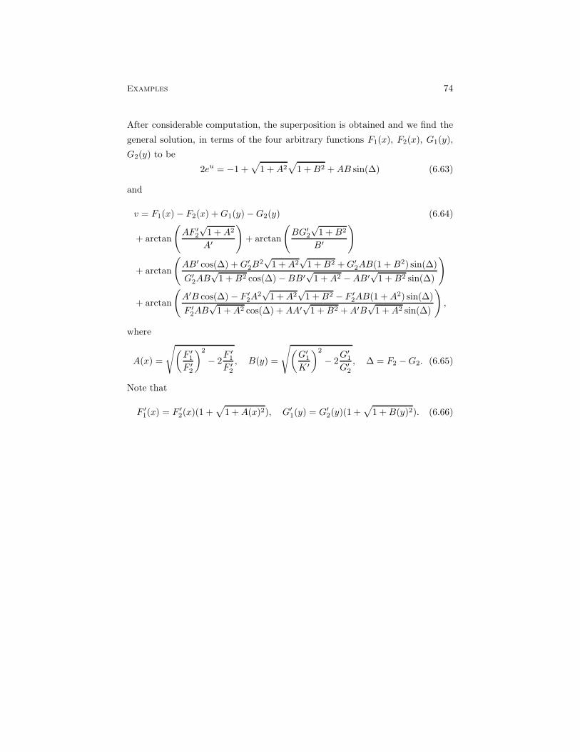
Examples 74

After considerable computation, the superposition is obtained and we find the

general solution, in terms of the four arbitrary functions F1(x), F2(x), G1(y),

G2(y) to be

2eu = −1 +√

1 +A2√

1 +B2 +AB sin(∆) (6.63)

and

v = F1(x) − F2(x) +G1(y) −G2(y) (6.64)

+ arctan

(

AF ′2

√1 +A2

A′

)

+ arctan

(

BG′2

√1 +B2

B′

)

+ arctan

(

AB′ cos(∆) +G′2B

2√

1 +A2√

1 +B2 +G′2AB(1 + B2) sin(∆)

G′2AB

√1 +B2 cos(∆) −BB′

√1 +A2 −AB′

√1 +B2 sin(∆)

)

+ arctan

(

A′B cos(∆) − F ′2A

2√

1 +A2√

1 +B2 − F ′2AB(1 +A2) sin(∆)

F ′2AB

√1 +A2 cos(∆) +AA′

√1 +B2 +A′B

√1 +A2 sin(∆)

)

,

where

A(x) =

√

(

F ′1

F ′2

)2

− 2F ′

1

F ′2

, B(y) =

√

(

G′1

K ′

)2

− 2G′

1

G′2

, ∆ = F2 −G2. (6.65)

Note that

F ′1(x) = F ′

2(x)(1 +√

1 +A(x)2), G′1(y) = G′

2(y)(1 +√

1 +B(y)2). (6.66)

Examples 75

Example 6.8. We turn now to some simple examples of overdetermined sys-

tems for a single unknown function of 3 independent variables, beginning with

the system

uxz = uux, uyz = uuy. (6.67)

The structure equations for the canonical encoding of this system as a rank 4

Pfaffian system I = α1, α2, α3, α4 on an 11-manifold are (modulo I), dα1 ≡ 0,

dα2 ≡ π1 ∧ π3 + π2 ∧ π4, dα3 ≡ π1 ∧ π4 + π2 ∧ π5, dα4 ≡ π1 ∧ π2, (6.68)

where π1 = dx, π2 = dy, π1 = dz,

π3 = duxx − (uxxu+ u2x) dz, π4 = duxy − (uxyu+ uyux) dz,

π5 = duyy − (uyyu+ u2y) dz, π2 = duzz − (uz + u2)(ux dx+ uy dy).

(6.69)

The first integrals for the singular Pfaffian systems V = I ∪ π1, . . . , π5 and

V = I ∪ π1, π2 are I1

= x, I2

= y, I1

= z,

I3

=uy

ux, I

4= DxI

3, I

5= Dy I

3, I

2= uz − u2/2, I

3= Dz I

2. (6.70)

The form π3 is not in V∞

+ V and therefore (6.67) is not Darboux integrable

on the 2-jet. The prolongation of (6.67) defines a decomposable rank 8 Pfaffian

system I [1] = α1, . . . , α8 on a 16 dimensional manifold. In addition to the

first integrals (6.70), we now also have

I6

= D2xI

3, I

7= DxyI

3, I

8= D2

y I3, I

9=uxxx

ux− 3u2

xx

2u2x

, I4

= D2z I

2(6.71)

and the conditions (1.8)–(1.10) for Darboux integrability of I [1] are now satisfied.

A 1-adapted coframe is σ1 = dI1, σ2 = dI

2, σ6 = dI

6, σ7 = dI

7, σ8 = dI

8,

σ9 = dI9, σ1 = dI

1, σ2 = dI

4,

η1 =1

uxα3 − uy

u2x

α2 = dI3 − I

4dI

1 − I5dI

2,

η2 =1

uxα6 − uy

u2x

α5 − uxx

u2x

α3 − uxyux − 2uyuxx

u3x

α2 = dI4 − I

6dI

1 − I7dI

2,

η3 =1

uxα7 − uy

u2x

α6 − uxy

u2x

α3 − −2uyuxy + uyyux

u3x

α2 = dI5 − I

7dI

1 − I8dI

2,

η1 = α4 − uα1 = dI2 − I

3dI

1, η2 = α8 − uα4 − uzα

1 = dI3 − I

4dI

1,

θ1 = α1 = du− ux dx− uy dy − uz dz,

θ2 = α2 = dux − uxx dx− uxy dy − uux dz,

θ3 = α3 = duxx − uxxx dx− uxxy dy − (uuxx + u2x) dz.

Examples 76

This frame is in fact 2-adapted. We next calculate U(∞)

= U ∪ X1, X2, X3and U

(∞)= U ∪ Y1, Y2, Y3, where

X1 = −uxI4∂θ1 − (uxxI

4+ uxI

6)∂θ2 − 3u2

xxI4

+ 4uxxuxI6 − 2u2

xI4I9

2ux∂θ3 ,

X2 = −ux∂θ3 , X3 = −ux∂θ1 − uxx∂θ2 − 3u2xx + 2u2

xI9

2ux∂θ3 , Y1 = −∂θ1, (6.72)

Y2 = u∂θ1 + ux∂θ2 + uxx∂θ3 , Y3 = (−u2

2+ I

2)∂θ1 − uux∂θ2 − (u2

x + uuxx)∂θ3 .

For the computations of Section 4.3 we use the base point defined by setting

u = 0, ux = 1, uxx = 0, I6

= 1, and all other first integrals (6.70)–(6.71) to 0,

The matrices (4.33) and (4.36) are then given by

P =

1

I6

2I4I9

I6 − I

4

I6

0 1 0

0 −I91

and R =

0 −1 0

I2

0 1

1 0 0

. (6.73)

From these matrices we calculate the 4 adapted coframes

θ1X =uxx

u2x

θ1 − 1

uxθ2, θ1Y = −u

2x + uuxx

u3x

θ2 +u

u2x

θ3,

θ2X = −u2xx

2u3x

θ1 +2uxx

u2x

θ2 − 1

uxθ3, θ2Y =

uxx

u3x

θ2 − 1

u2x

θ3, (6.74)

θ3X = − 1

uxθ1, θ3Y = −θ1 +

u(2u2x + uuxx)

2u3x

θ2 − u2

2u2x

θ3.

The Vessiot algebra is sl(2). Because this algebra is semi-simple, we can use

Case I of Section 4.4, Theorem 5.1, and (6.74) to directly determine the map

ρ : M → Aut(sl(2) as

ρ(u, ux, uxx) = λ =

u2x − uuxx

u2x

− u

ux−uxx(uuxx − 2u2

x)

2u3x

uxx

u2x

1

ux

u2xx

2u3x

u(uuxx − 2u2x)

2u2x

u2

2ux

(uuxx − 2ux)2

4u3x

. (6.75)

To obtain the superposition formula we introduce local coordinates (z, w,

wx, wxx, wz , wzz , wzzz) for M1 and (x, y, v, vx, vy, vz, vxx, vxy, vyy, vyz, vxxx,

Examples 77

vxxy, vxyy, vyyy, vyyz) for M2. The inclusions ι1 : M1 → M and ι2 : M2 → M

are fixed by

ι1(wI) = uI , ι∗1(Ia) = 0, ι2(vI) = uI , ι∗2(I

a) = 0.

The superposition formula is then found by solving the equations

ι∗1(Ia) = I

a, ι∗2(I

a) = I

a, ρ(u, ux, uxx) = ρ(w,wx, wxx) ·ρ(v, vx, vxx) (6.76)

for the coordinates of M . We find that

u = w − 2vw2x

−2wx + vwxx. (6.77)

Finally, we calculate the integral manifolds for W and W . It is immediate

that W is the canonical Pfaffian system on J3(R,R2) and hence the integral

manifolds are defined by v = V (x, y). The last non-zero form in the derived flag

for

W = dw − wzdz, dwz − wzz dz, dwzz − wzzz dz, dwx − wxwdz,

dwxx + (−w2x − wwxx)dz

yields the Pfaffian equation

dwxx − wxx

wxdwx − w2

xdz = 0

from which it follows that wx = G′(z) and wxx = G(z)G′(z). One of the

remaining equations in W then gives w = G′′(z)/G′(z). On replacing V (x, y)

by −2/F (x, y), the superposition formula (6.77) becomes

u(x, y, z) =G′′(z)

G′(z)− 2G′(z)

F (x, y) +G(z), (6.78)

which gives the general solution to (6.67).

We continue this example by considering two variations on (6.67). First we

observe that to (6.67) we may add any equation of the form

F (x, y,uy

ux,uyuxx − uxuxy

ux,uyuxy − uxutyy

u2x

) = 0 (6.79)

to obtain a rank 4 Pfaffian system I = α1, α2, α3, α4 on a 10 dimensional

manifold. The structure equations become ( mod I) dα1 ≡ 0,

dα2 ≡ π1 ∧ π2, dα3 ≡ π3 ∧ π4, dα4 ≡ π1 ∧ π2 (6.80)

Examples 78

and hence all such systems are involutive with Cartan character s1 = 3.

For example, consider the system of 3 equations

uyuxy − uxuyy = 0, uxz = uux, uyz = uuy (6.81)

The foregoing calculations can be repeated, almost without modification, to

arrive at the same superposition formula (6.77) – the only difference is that now

W is the (prolonged) canonical Pfaffian system for the equation vyvxy−vxvyy =

0, an equation which is itself Darboux integrable. Thus, in more complicated

situations, the method of Darboux, can be used to integrate the Pfaffian systems

W and W and the superposition formula for the original system is given by a

composition of superposition formulas. In the case of the present example,

the calculation of the first integrals for W reveals that this system is contact

equivalent to the wave equation (via X = x, Y = v, V = y, VX = −vx/vy,

VY = 1/vy) and leads to the parametric solution

x = σ, y = f(σ) + g(τ), u =G′′(z)

G′(z)− 2G′(z)

τ +G(z). (6.82)

Our second variation of (6.67) is obtained by the differential substitution

ux = exp(v). This leads to the equations

vxz = exp(v) and vyzz = vyzvz . (6.83)

It is surprising that the canonical Pfaffian system for these equations (obtained

by the restriction of the contact ideal on J3(R,R2)) does not define a decom-

posable Pfaffian system. The following theorem resolves this difficulty.

Theorem 6.9. The system of differential equations

uxz = F (x, y, z, u, uz, uyz, uzz),

uyzz = G(x, y, z, u, ux, uy, uz, uyz, uzz, uyyz, uzzz)(6.84)

determines the rank 4 Pfaffian system

α1 = du− uxdx− uydy − uzdz, α2 = duz − Fdx− uyzdy − uzzdz,

α3 = duyz −Dy(F )dx − uyyzdy −Gdz,

α4 = duzz −Dz(F )dx −Gdy − uzzzdz,

(6.85)

on an 11 dimensional manifold. If the compatiblity conditions for (6.84) hold,

then this Pfaffian system is decomposable and involutive with Cartan characters

s1 = 1 and s2 = 1.

Examples 79

We use Theorem 6.9 to write (6.83) as a rank 4 Pfaffian system on an 11-

manifold. The prolongation of this system is Darboux integrable and calcula-

tions, virtually identical to those provided for (6.67), lead directly to the general

solution

v(x, y, z) = ln( 2Fx(x, y)G′(z)

(F (x, y) +G(z))2)

. (6.86)

References

[1] I. M. Anderson and M. E. Fels, Exterior Differential Systems with Symmetry, Acta. Appl.

Math. 87 (2005), 3–31.

[2] I. M. Anderson and M. Juras, Generalized Laplace Invariants and the Method of Darboux,

Duke J. Math 89 (1997), 351–375.

[3] B. M. Barbashov, V. V. Nesterenko, and A. M. Chervyakov, General solutions of nonlin-

ear equations in the geometric theory of the relativistic string, Commun. Math Physics

84 (1982), 471–481.

[4] F. De Boer, Application de la methode de Darboux a l’integration de l’equation

differentielle s = f(r,t)., Archives Neerlandaises 27 (1893), 355–412.

[5] R. L Bryant and P. A. Griffiths, Characteristic cohomology of differential systems (I),

Selecta Math. (N.S.) 1 (1995), 21–112.

[6] R. L. Bryant, P. A. Griffiths, and L. Hsu, Hyperbolic exterior differential systems and

their conservation laws, Parts I and II, Selecta Math., New series 1 (1995), 21–122 and

265–323.

[7] E Cartan, Les systemes de Pfaff a cinq variables et les equations aux derivees partielles

du second ordre, Ann. Sci. Ecole Norm. 3 (1910), no. 27, 109–192.

[8] , Sur les systemes en involution d’equations aux deriv’ees partielles du second

ordre a une fonction inconnue de trois variable independantes, Bull Soc. Math France

39 (1911), 352-443.

[9] G. Darboux, Lecons sur la theorie generale des surfaces et les applications geometriques

du calcul infinitesimal, Gauthier-Villars, Paris, 1896.

[10] P. T. Eendebak, Contact Structures of Partial Differential Equations, 2007.

[11] H. Flanders, Differential Forms with Applications to the Physical Sciences, Dover, New

York, 1963.

[12] M. E. Fels and P. J. Olver, Moving coframes I. A practical algorithm, Acta. Appl. Math.

51 (1998), 161-213.

[13] A. Forsyth, Theory of Differential Equations, Vol 6, Dover Press, New York, 1959.

[14] A. Gonzalez-Lopez, N. Kamran, and P. J. Olver, Lie algebras of vector fields in the real

plane, Proc. London Math. Soc. 64 (1992), 339-368.

[15] E. Goursat, Lecon sur l’integration des equations aux deriees partielles du second ordre

a deux variables independantes, Tome 1, Tome 2, Hermann, Paris, 1897.

Examples 80

[16] E. E. Goursat, Recherches sur quelques equations aux deriees partielles du second ordre,

Ann. Fac. Sci. Toulouse 1 (1899), 31–78 and 439–464.

[17] P. Griffiths, On Cartan’s method of Lie groups and moving frames as applied to unique-

ness and existence questions in differential geometry, Duke Math. J. 41 (1974), 775–814.

[18] S.S. Kobyashi and K. Nomizu, Foundations of Differential Geometry, John Wiley, 1963.

[19] A. N. Leznov and M. V. Saleliev, Representation theory and integration of nonlinear

spherically symmetric equations to gauge theories, Commun. Math. Phys. 74 (1980),

111-118.

[20] , Two-dimensional exactly and completely integrable dynamical systems, Com-

mun. Math. Phys. 89 (1983), 59–75.

[21] P. J. Olver, Equivalence, Invariants, and Symmetry (1995).

[22] V. V. Sokolov and A. V. Ziber, On the Darboux integrable hyperbolic equations, Phys

Lett. A 208, 303–308.

[23] S Sternberg, Lectures on Differential Geometry, Second, Chelsa, New York, 1984.

[24] O. Stormark, Lie’s structural approach to PDE systems 80 (2000).

[25] V. S. Varadarajan, Lie Groups, Lie Algebras and Their Representations, Springer-Verlag,

New York, 1984.

[26] P. J. Vassiliou, Vessiot structure for manifolds of (p, q)-hyperbolic type: Darboux integra-

bility and symmetry, Trans. Amer. Math. Soc. 353 (2001), 1705–1739.

[27] E. Vessiot, Sur les equations aux derivees partielles du second ordre, F(x,y,z,p,q,r,s,t)=0,

integrables par la methode de Darboux, J. Math. Pure Appl. 18 (1939), 1–61.

[28] , Sur les equations aux derivees partielles du second ordre, F(x,y,z,p,q,r,s,t)=0,

integrables par la methode de Darboux, J. Math. Pure Appl. 21 (1942), 1–66.