superior guarantees for sequential prediction and lossless

Journal of Machine Learning Research 7 (2006) 379–411 Submitted 8/05; Published 2/06

Superior Guarantees for Sequential Predictionand Lossless Compression via Alphabet Decomposition

Ron Begleiter [email protected]

Ran El-Yaniv [email protected] of Computer ScienceTechnion - Israel Institute of TechnologyHaifa 32000, Israel

Editor: Dana Ron

Abstract

We present worst case bounds for the learning rate of a known prediction method that is based onhierarchical applications of binary context tree weighting (CTW) predictors. A heuristic applicationof this approach that relies on Huffman’s alphabet decomposition is known to achieve state-of-the-art performance in prediction and lossless compression benchmarks. We show that our newbound for this heuristic is tighter than the best known performance guarantees for prediction andlossless compression algorithms in various settings. Thisresult substantiates the efficiency of thishierarchical method and provides a compelling explanationfor its practical success. In addition, wepresent the results of a few experiments that examine other possibilities for improving the multi-alphabet prediction performance of CTW-based algorithms.

Keywords: sequential prediction, the context tree weighting method,variable order Markov mod-els, error bounds

1. Introduction

Sequence prediction and entropy estimation are fundamental tasks in numerous machine learningand data mining applications. Here we consider a standard discrete sequence prediction settingwhere performance is measured via the log-loss (self-information). It is well known that this settingis intimately related to lossless compression, where in fact high quality predictionis essentiallyequivalent to high quality lossless compression.

Despite the major interest in sequence prediction and the existence of a number of universalprediction algorithms, some fundamental issues related to learning from finite (and small) samplesare still open. One issue that motivated the current research is that the finite-sample behavior ofprediction algorithms is still not sufficiently understood.

Among the numerous compression and prediction algorithms there are very few that offer bothfinite sample guarantees and good practical performance. Thecontext tree weighting(CTW) methodof Willems et al. (1995) is a member of this exclusive family of algorithms. TheCTW algorithm isan “ensemble method,” mixing the predictions of many underlying variable order Markov models(VMMs), where each such model is constructed using zero-order conditional probability estimators.The algorithm isuniversalwith respect to the class of bounded-order VMM tree-sources. Moreover,the algorithm has a finite sample point-wise redundancy bound (for any particular sequence).

c©2006 Ron Begleiter and Ran El-Yaniv.

BEGLEITER AND EL-YANIV

The high practical performance of the originalCTW algorithm is most apparent when applied tobinaryprediction problems, in which case it uses the well-known (binary) KT-estimator (Krichevskyand Trofimov, 1981). When the algorithm is applied to non-binary prediction/compression problems(using the multi-alphabet KT-estimator), its empirical performance is mediocre compared to the bestknown results (Tjalkens et al., 1997). Nevertheless, a cleveralphabet decompositionheuristic, sug-gested by Tjalkens et al. (1994) and further developed by Volf (2002), does achieve state-of-the-artcompression and prediction performance on standard benchmarks (see, e.g., Volf, 2002; Sadakaneet al., 2000; Shkarin, 2002; Begleiter et al., 2004). In this approach themulti-alphabet problemis hierarchically decomposed into a number of binary prediction problems. Weterm the resultingprocedure “theDECO algorithm.” Volf suggested applying theDECO algorithm using Huffman’stree as the decomposition structure, where the tree construction is based onletter frequencies. Weare not aware of any previous compelling explanation for the striking empirical success ofDECO.

Our main contribution is a general worst case redundancy bound for algorithm DECO appliedwith any alphabet decomposition structure. The bound proves that the algorithm is universalwithrespect to VMMs. A specialization of the bound to the case of Huffman decompositions results in atight redundancy bound. To the best of our knowledge, this new boundis the sharpest available forprediction and lossless compression for sufficiently large alphabets and sequences.

We also present a few empirical results that provide some insight into the following questions:(1) Can we improve on the Huffman decomposition structure using an optimized decompositiontree? (2) Can other, perhaps “flat” types of alphabet decomposition schemes outperform the hierar-chical approach? (3) Can standardCTW multi-alphabet prediction be improved with other types of(non-KT) zero-order estimators?

Before we start with the technical exposition, we introduce some standard terms and definitions.Throughout the paper,Σ denotes a finite alphabet withk = |Σ| symbols. Suppose we are givena sequencexn

1 = x1x2 · · ·xn. Our goal is to generate a probabilistic predictionP(xn+1|xn1) for the

next symbol given the previous symbols. Clearly this is equivalent to beingable to estimate theprobability P(xn

1) of any complete sequence, sinceP(xn+1|xn1) = P(xn+1

1 )/P(xn1) (provided that the

marginality condition∑σ P(xn1σ) = P(xn

1) holds).We consider a setting where the performance of the prediction algorithm is measured with re-

spect to the best predictor in some reference, which we call here acomparison class. In our casethe comparison class is the set of all variable order Markov models (see details below). LetALG bea prediction algorithm that assigns a probability estimatePALG(xn

1) for any givenxn1. The point-

wise redundancyof ALG with respect to the predictorP and the sequencexn1 is RALG(xn

1,P) =logP(xn

1)− logPALG(xn1). The per-symbol point-wise redundancy is1

nRALG(xn1,P). ALG is called

universalwith respect to a comparison classC , if

limn→∞

supP∈C

maxxn

1

1n

RALG(xn1,P) = 0. (1)

2. Preliminaries

This section presents the relevant technical background for the present work. The contextual back-ground appears in Section 7. We start by presenting the class oftree sources. We then describethe CTW algorithm and discuss some of its known properties and performance guarantees. Finally,we conclude this section with a description of theDECO method for predicting multi-alphabet se-quences using binaryCTW predictors.

380

SUPERIORGUARANTEES FORSEQUENTIAL PREDICTION AND LOSSLESSCOMPRESSION

2.1 Tree Sources

The parametric distribution estimated by theCTW algorithm is the set of depth-bounded tree-sources. A tree-source is a variable order Markov model (VMM). LetΣ be an alphabet of sizek andD a non-negative integer. AD-bounded tree sourceis any full k-ary tree1 whose height≤ D.Each leaf of the tree is associated with a probability distribution overΣ. For example, in Figure 1we depict three tree-sources over a binary alphabet. In this case, the trees are full binary trees. Thesingle node tree in Figure 1(c) is a zero-order (Bernoulli) source and the other two trees (Figure 1(a)and (b)) are 2-bounded sources. Another useful way to view a tree-source is as a setS ⊆ Σ≤D of“suffixes” in which eachs∈ S is a path (of length up toD) froma (unique) leaf to the root. We alsorefer toS as the (tree-source)topology. For example,S = {0,01,11} in Figure 1(b). The path fromthe middle leaf to the root corresponds to the sequences= 01 and therefore we refer to this leafsimply ass. For convenience we also refer to an internal node by the (unique) pathfrom that nodeto the root. Observe that this path is a suffix of somes∈ S . For example, the right child of the rootin Figure 1(b) is denoted by the suffix1.

The (zero-order) distribution associated with the leafs is denotedzs(σ), ∀σ∈Σ, where∑σ zs(σ)=1 andzs(·) ≥ 0.

(a) (b) (c)ε

0

(.5, .5)

0

(.15, .85)

1

1

(.7, .3)

0

(.55, .45)

1

ε

(.25, .75)

0 1

(.35, .65)

0

(.12, .88)

1

ε

(.25, .75)

Figure 1: Three examples forD = 2 bounded tree-sources overΣ = {0,1}. The correspond-ing suffix-sets areS(a) = {00,10,01,11}, S(b) = {0,01,11}, and S(c) = {ε} (ε is theempty sequence). The probabilities for generatingx3

1 = 100 given initial context00areP(a)(100|00) = P(a)(1|00)P(a)(0|01)P(a)(0|10) = 0.5·0.7·0.15,P(b)(100|00) = 0.75·0.35·0.25, andP(c)(100|00) = 0.75·0.25·0.25.

We denote the set of allD-bounded tree-source topologies (suffix sets) byCD. For example,C0 = {{ε}} andC1 = {{ε}, {0,1}}, whereε is the empty sequence.

For eachn, a D-bounded tree-source induces a probability distribution over the setΣn of all n-length sequences. This distribution depends on an initial “context” (or “state”), x0

1−D = x1−D · · ·x0,which can be any sequence inΣD. The tree-source induced probability of the sequencexn

1 =x1x2 · · ·xn is, by the chain rule,

PS (xn1) =

n

∏t=1

PS (xt |xt−1t−D), (2)

wherePS (xt |xt−1t−D) is zs(xt) = PS (xt |s) ands is the (unique) suffix ofxt−1

t−D in S . Clearly, a tree-source can generate sequences: theith symbol is randomly drawn using the conditional distribution

1. A full k-ary tree is a tree in which each node has exactly zero ork children.

381


PS (·|xi−1i−D). Let SUBs(xn

1) be theorderednon-contiguous sub-sequence of symbols appearing afterthe contexts in xn

1. For example, ifx81 = 01100101, ands= 0, then,SUBs(x8

1) = 1011. Let sbe anysuffix in S andym

1 = SUBs(xn1). For everyxn

1 6= ε we definezs(xn1) = ∏m

i=1zs(yi) and for the emptysequencezs(ε) = 1. Thus, we can rewrite Equation (2) as

PS (xn1) = ∏

s∈S

zs(xn1). (3)

2.2 The Context-Tree Weighting Method

Here we describe theCTW prediction algorithm (Willems et al., 1995), originally presented as alossless compression algorithm.2 The goal of theCTW algorithm is to predict a sequence (nearly)as good as the the best tree-source. This goal can be divided into two sub-problems. The first is toguess the topology of the best tree-source, and the second is to estimate thedistributions associatedwith its leaves.

Suppose, first, that the best tree topology (i.e., the suffix-setS ) is known. A good solutionassigns to eachs∈ S a zero-order estimatorzs that estimates the true probability distributionzs

associated withs. This can be done using standard statistical methods; that is, by considering alloccurrences ofs in xn

1 and constructing ˆzs via counting and smoothing. We currently consider ˆzs asa generic estimator and discuss specific implementations later on.

In practice, however, the best tree-source’s topology is unknown. Instead of guessing this topol-ogy, CTW considers all possibleD-bounded topologiesS (each is a subtree of the perfectk-arytree), and for eachS it constructs a predictor by estimating its zero-order leaf probabilities.CTW

then takes a weighted mixture of all these predictors, corresponding to all topologies. Clearly, thereare exponentially manyD-bounded topologies. The beauty of theCTW algorithm is the efficientcomputation of this mixture of exponential size.

In the following description of theCTW algorithm, the output of the algorithm is a probabilityPCTW(xn

1) for the entire sequencexn1. Observe that this is equivalent to estimating the next-symbol

probabilities becausePCTW(σ|xn

1) = PCTW(xn1σ)/PCTW(xn

1) (4)

for eachσ∈Σ (provided that these probabilities can be marginalized, i.e.,∑σ PCTW(xn1σ)= PCTW(xn

1)).We require the following definitions. Letxn

1 be any sequence (inΣn) and fix a boundD andan initial contextx0

1−D. Let s be any context inS , andym1 = SUBs(xn

1). Thesequentialzero-orderestimation forxn

1 is, by the chain-rule,

zs(xn1) =

m

∏i=1

z(yi |yi−11 ), (5)

wherey01 = ε and z(yi |yi−1

1 ) is a zero-order probability estimate based on the symbol counts inyi−1

1 . The product of such predictions is ˆzs(xn1), and hence, we refer to it as a sequential zero-order

estimate.We now describe the mainCTW idea via a simple example and then provide a pseudo-code for

the generalCTW algorithm. Consider a binary alphabet and the caseD = 1. Here,CTW works onthe perfect binary tree of height one and therefore should mix the predictions associated with two

2. As mentioned above, any lossless compression algorithm can be translated into a sequence prediction algorithm andvice versa (see, e.g., Merhav and Feder, 1998).

382


topologies:S0 = {ε} (whereε is the empty sequence), andS1 = {0,1}. Note thatS0 correspondsto the zero-order topology as in Figure 1(c). The algorithm takes a mixture of the zero-order esti-matezε(xn

1) and the one-order estimate. The latter is exactly ˆz0(xn1) · z1(xn

1) because ˆz0 andz1 areindependent. Thus, the final estimate is

PCTW(xn1) =

12zε(xn

1)+12

(z0(xn1) · z1(xn

1)) .

For larger trees (D > 1), CTW uses the same idea, but now, instead of taking zero-order estimatesfor the root’s children, theCTW algorithm recursively computes their estimates. The pseudo-codeof the CTW recursive mixture computation appears in Algorithm 1. We later show in Lemma 3that this code calculates the mixture of allD-bounded tree-source predictions weighted by theircomplexities, which are defined as follows.

Algorithm 1 The context-tree weighting algorithm

/* This code calculates theCTW probability for the (whole) sequencexn1, PCTW(xn

1|x01−D). The input argu-

ments include the sequencexn1, an initial contextx0

1−D (that determines the suffixes for predicting the firstsymbols), a bound D on the order, and an implementation for the sequential zero-order estimatorszs(·).The code uses themix procedure (see below).*/

CTW(xn1, x0

1−D, D, zs(·)) {for everys∈ Σ≤D do

calculate and store ˆzs(xn1) as given in Equation (5).

end forreturn PCTW(xn

1) = mix(ε,xn1,x

01−D).

}

/* This procedure mixes the predictions of all continuations s′s of s∈ Σ≤D, such that s′s is also inΣ≤D.Note that the context of the first few symbols is determined bythe initial contextx0

1−D. */mix (s,xn

1,x01−D) {

if |s| = D thenreturn zs(xn

1).else

return 12 zs(xn

1)+ 12 ∏σ∈Σ mix(σs,xn

1,x01−D).

end if}

Definition 1 Let TS denote the tree associated with the suffix setS . The complexityof TS is definedto be

|TS | = |{s∈ S : |s| < D}|+ |S |−1k−1

.

Recall that the number of leaves in TS is exactly|S | and there are|S |−1k−1 internal nodes in any full

k-ary tree. Therefore,|TS | is the number of nodes in TS minus the number of leaves s∈ S withmaximal depth D.

For example, letT(a) be the tree of Figure 1(a) (resp. for(b) and(c)); |T(a)| = 0+ 3 = 3; |T(b)| =1+2 = 3 (= |T(a)); |T(c)| = 1+0 = 1.

383


Observation 2 Let Sσ = {s : sσ ∈ S}. For any D-bounded topologyS , |S | > 1,

|TS | = 1+ ∑σ∈Σ

|TSσ |.

Note thatSσ is a(D−1)-bounded topology. Note also that the complexity depends on D. Therefore,for the base case (when|S | = 1), the complexity of TS is zero if D= 0 and one if D≥ 1.

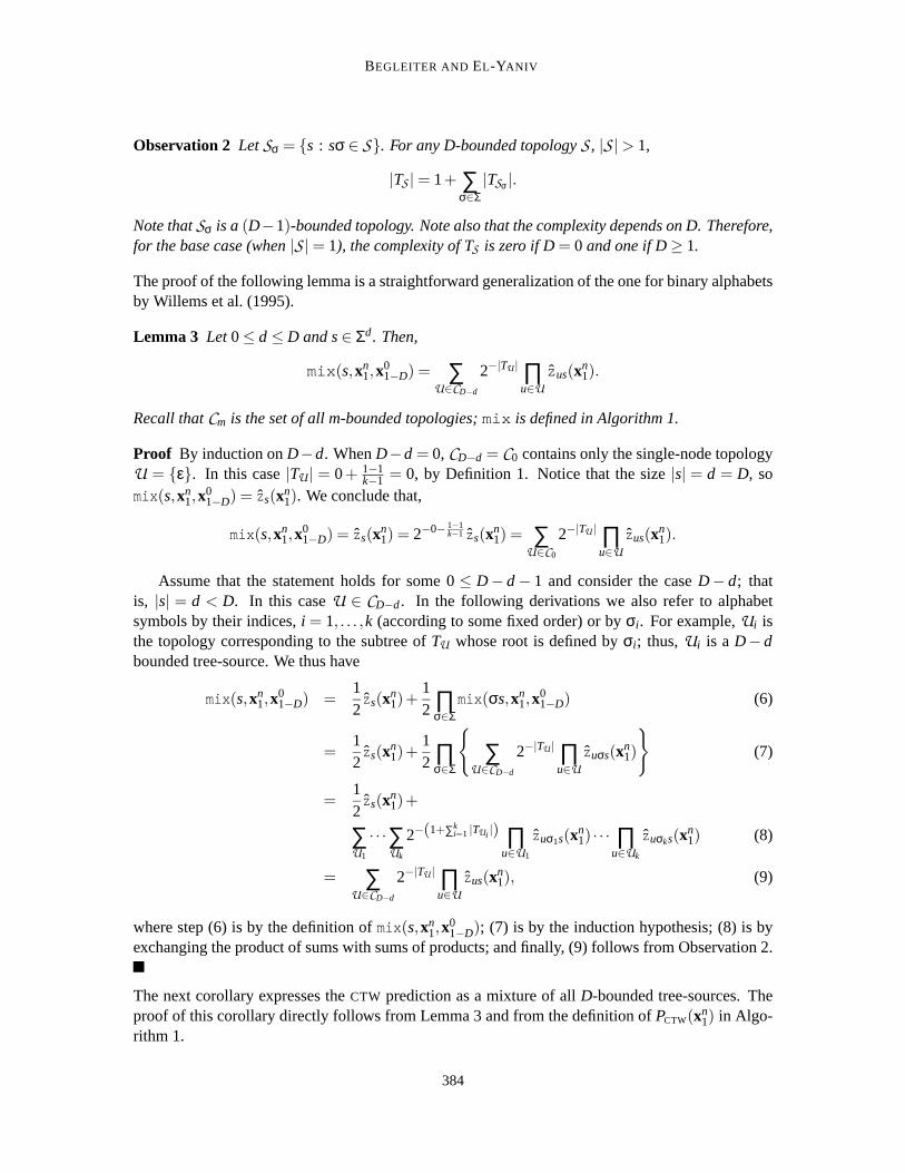
The proof of the following lemma is a straightforward generalization of the onefor binary alphabetsby Willems et al. (1995).

Lemma 3 Let0≤ d ≤ D and s∈ Σd. Then,

mix (s,xn1,x

01−D) = ∑

U∈CD−d

2−|TU | ∏u∈U

zus(xn1).

Recall thatCm is the set of all m-bounded topologies;mix is defined in Algorithm 1.

Proof By induction onD−d. WhenD−d = 0, CD−d = C0 contains only the single-node topologyU = {ε}. In this case|TU | = 0+ 1−1

k−1 = 0, by Definition 1. Notice that the size|s| = d = D, somix(s,xn

1,x01−D) = zs(xn

1). We conclude that,

mix(s,xn1,x

01−D) = zs(xn

1) = 2−0− 1−1k−1 zs(xn

1) = ∑U∈C0

2−|TU | ∏u∈U

zus(xn1).

Assume that the statement holds for some 0≤ D− d− 1 and consider the caseD− d; thatis, |s| = d < D. In this caseU ∈ CD−d. In the following derivations we also refer to alphabetsymbols by their indices,i = 1, . . . ,k (according to some fixed order) or byσi . For example,Ui isthe topology corresponding to the subtree ofTU whose root is defined byσi ; thus,Ui is a D−dbounded tree-source. We thus have

mix(s,xn1,x

01−D) =

12zs(xn

1)+12 ∏

σ∈Σmix(σs,xn

1,x01−D) (6)

=12zs(xn

1)+12 ∏

σ∈Σ

{

∑U∈CD−d

2−|TU | ∏u∈U

zuσs(xn1)

}

(7)

=12zs(xn

1)+

∑U1

· · ·∑Uk

2−(1+∑ki=1 |TUi |) ∏

u∈U1

zuσ1s(xn1) · · · ∏

u∈Uk

zuσks(xn1) (8)

= ∑U∈CD−d

2−|TU | ∏u∈U

zus(xn1), (9)

where step (6) is by the definition ofmix(s,xn1,x

01−D); (7) is by the induction hypothesis; (8) is by

exchanging the product of sums with sums of products; and finally, (9) follows from Observation 2.

The next corollary expresses theCTW prediction as a mixture of allD-bounded tree-sources. Theproof of this corollary directly follows from Lemma 3 and from the definition ofPCTW(xn

1) in Algo-rithm 1.

384


Corollary 4PCTW(xn

1) = mix (ε,xn1,x

01−D) = ∑

S∈CD

2−|TS |∏s∈S

zs(xn1). (10)

Remark 5 The number of tree-source topologies inCD is superexponential (recall that eachS ∈ C

is a pruning of the perfect k-ary tree of height D). Thus, for practical reasons, the calculation ofEquation (10) must be efficient. The pseudo-code of theCTW in Algorithm 1 is conceptual ratherthan efficient. However, the beauty of theCTW is that it can calculate the tree-source mixture inlinear time with respect to n. For a description of an efficient implementation of theCTW algorithm,see for example, Sadakane et al. (2000) and Chapter 4.4 of Volf (2002). Our Java implementationof theCTW algorithm can be found athttp://www.cs.technion.ac.il/˜rani/code/vmm.

2.3 Analysis of CTW for Multi-Alphabets

The analysis ofCTW for multi-alphabets (multi-CTW) relies upon specific implementations of thesequential zero-order estimators ˆzs(·). Such estimators are in general counters of past events. How-ever, these estimators should not neglect unobserved events. In the context of log-loss prediction,assigning zero probability to these “zero frequency” events is harmful because the log-loss of anunobserved but possible event is infinite. The problem of assigning probability mass to unobservedevents is also called the “missing-mass problem” (or the “zero frequency problem”).

The originalCTW algorithm applies the well-knownKT estimator (Krichevsky and Trofimov,1981).

Definition 6 Fix anyxn1 and let Nσ be the frequency ofσ ∈ Σ in xn

1. TheKT estimator assigns thefollowing (sequential zero-order) probability to the sequencexn

1,

z KT(xn1) = z KT(xn−1

1 )Nxn +1/2

∑σ∈Σ Nσ +k/2, (11)

wherez KT(ε) = 1.

Observe that the termP(σ|xn1) = Nσ+1/2

∑σ∈Σ Nσ+k/2, is anadd-half predictor that belongs to the family of

add-constant predictors.3

TheKT estimator provides a prediction that is uniformly close to the setZ of zero-order distri-butions overΣ. Each distributionz ∈ Z is a probability vector from(

�+)k, andz(σ) denotes the

probability ofσ. Thus,z(xn1) = ∏σ z(σ)Nσ . The next theorem provides a performance guarantee on

the worst-case redundancy of theKT estimator. This guarantee is for a whole sequencexn1. Notice

that the per-symbol redundancy ofKT diminishes withn at a ratelognn . For completeness, the proof

of the following theorem is provided in Appendix A.

Theorem 7 (Krichevsky and Trofimov) LetΣ be any alphabet with|Σ|= k≥ 2. For any sequencexn

1 ∈ Σn,

RKT(xn1) = logsup

z∈Z

z(xn1)− logz KT(xn

1) ≤k−1

2logn+ logk. (12)

3. Another famous add-constant predictor is the add-one predictor, also calledLaplace’s law of succession(Laplace,1995).

385


Remark 8 Krichevsky and Trofimov (1981) originally definedKT to be a mixture of all zero-orderdistributions inZ, weighted by the Dirichlet (1/2) distribution. Thus, this mixture is

z KT(xn1) =

Z

Z

w(dz)z(xn1),

where w(dz) is the Dirichlet distribution with parameter1/2 defined by

w(dz) =1√k

Γ( k2)

Γ(12)k

k

∏i=1

z(i)−1/2λ(dz), (13)

Γ(x) =R�

+ tx−1exp(−t)dt is the gamma function (see, for example, Courant and John, 1989), andλ(·) is a measure onZ. Shtarkov (1987) was the first to show that this mixture can be calculatedsequentially as in Definition 6.

The upper bound of Theorem 7 on the redundancy of theKT estimator is a key element inthe proof of the following theorem, providing a finite-sample point-wise redundancy bound for themulti-CTW (see, e.g., Tjalkens et al., 1993; Catoni, 2004).

Theorem 9 (Willems et al.) LetΣ be any alphabet with|Σ|= k≥ 2. For any sequencexn1 ∈ Σn and

any D-bounded tree-source with a topologyS and distribution PS , the following holds:

RCTW(xn1,PS ) ≤

{

nlogk+ k|S |−1k−1 , n < |S |;

(k−1)|S |2 log n

|S | + |S | logk+ k|S |−1k−1 , n≥ |S |.

Proof

RCTW(xn1,PS ) = logPS (xn

1)− logPCTW(xn1)

= logPS (xn

1)

∏s∈S zs(xn1)

︸︷︷︸

(i)

+ log∏s∈S zs(xn

1)

PCTW(xn1)

︸︷︷︸

(ii)

(14)

We now bound the term (14)(i) and define the following auxiliary function:

f (x) =

{

xlogk ,0≤ x < 1;k−1

2 logx+ logk ,x≥ 1.

386


Note that this function is continuous and concave in[0,∞). Let Nσ(s) denote the frequency ofσ inSUBs(xn

1). Thus,

logPS (xn

1)

∏s∈S zs(xn1)

= ∑s∈S

logzs(xn

1)

zs(xn1)

(15)

≤ ∑s∈S , s.t.

∑Nσ(s)>0

(

k−12

log(∑σ

Nσ(s))+ logk

)

(16)

= |S |∑s∈S

1|S | f (∑

σNσ(s))

≤ |S | f (∑s∈S ∑σ Nσ(s)|S | ) (17)

= |S | f ( n|S |)

=

{

nlogk, n < |S |;(k−1)|S |

2 log n|S | + |S | logk, n≥ |S |, (18)

where step (15) follows from an application of Equation (3); step (16) is by the performance guar-antee for theKT prediction, as given in Theorem 7; and step (17) is by Jensen’s inequality.

We now bound the term (14)(ii )

log∏s∈S zs(xn

1)

PCTW(xn1)

= log∏s∈S zs(xn

1)

∑S∈CD2−|TS | ∏s∈S zs(xn

1)(19)

≤ log∏s∈S zs(xn

1)

∑S∈CD2−

k|S |−1k−1 ∏s∈S zs(xn

1)(20)

≤ log∏s∈S zs(xn

1)

2−k|S |−1

k−1 ∏s∈S zs(xn1)

= log2k|S |−1

k−1

=k|S |−1

k−1, (21)

where in step (19) we applied Equation (10) and the justification for (20) is that |{s∈ S : |s| < D}| ≤|S |. Thus, according to Definition 1,|TS | ≤ |S |+ |S |−1

k−1 = k|S |−1k−1 . We complete the proof by summing

up (18) and (21).

Remark 10 TheCTW bound used by Catoni (2004) is somewhat tighter than the bound of Theo-rem 9 but contains some implicit terms.

Remark 11 Willems (1998) provided extensions for theCTW algorithm that eliminate its depen-dency on the maximal bound D and the initial contextx0

1−D. For the extended algorithm and binaryprediction problems, Willems derived a point-wise redundancy bound of

|S |2

logn−∆s(xn

1)

|S | +2|S |−1+∆s(xn1),

387


where∆s(xn1)≤ D denotes the number of symbols in the prefix ofxn

1 that do not appear after a suffixs∈ S .

Remark 12 Interestingly, it can be shown that theCTW algorithm is an instance of the well-knowngenericexpert-advicealgorithm of Vovk (1990). This observation is new, to the best of our knowl-edge, although there are citations that connect theCTW algorithm with the expert-advice scheme(see, e.g., Merhav and Feder, 1998; Helmbold and Schapire, 1997).

It can be shown that these two algorithms are identical when Vovk’s algorithm is applied withthe log-loss (see, e.g., Haussler et al., 1998, example 3.12). In this case, the set of experts inVovk’s algorithm consists of all D-bounded tree-sources,CD; the initial weight of each expert,S ,corresponds to its complexity|TS |; and the weight of each expert at round t equals2−|TS |PS (xt−1

1 ).Note, however, that the power of theCTW method is in its efficiency in mixing exponentially manysources (or experts). Vovk’s algorithm is not concerned with how to compute this average.

2.4 Hierarchical CTW Decompositions

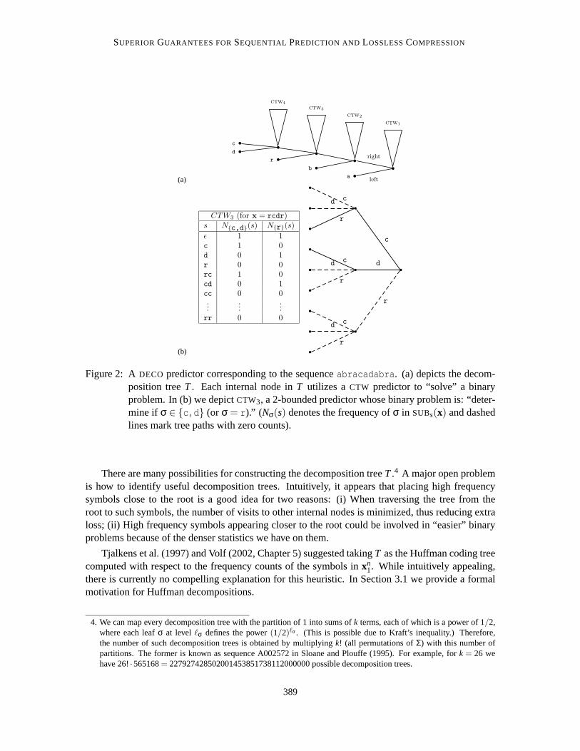
TheCTW algorithm is known to achieve excellent empirical performance inbinaryprediction prob-lems. However, when applyingCTW on sequences over larger alphabets, the resulting performancefalls short of the best known (Tjalkens et al., 1997). This fact motivatesdifferent approaches forapplying theCTW algorithm on multi-alphabet sequences. Volf targeted this issue in his Ph.D. the-sis (2002). Following Tjalkens et al. (1994), who proposed a rudimentary alphabet decompositionapproach, he studied a solution to the multi-alphabet prediction problem that isbased on a tree hi-erarchy of binary problems. Each of these binary problems is solved using a slight variation of thebinaryCTW algorithm. We now describe the resulting ‘decomposedCTW’ approach, which we termfor short the “DECO” algorithm.

Consider a full binarydecomposition tree Twith k = |Σ| leaves, where each leaf is uniquelyassociated with a symbol inΣ. Each internal nodev of T corresponds to the binary problem ofpredicting whether the next symbol is a leaf onv’s left subtree or a leaf onv’s right subtree. For ex-ample, forΣ = {a,b,c,d,r}, Figure 2 depicts a decomposition treeT such that its root correspondsto the problem of predicting whether the next symbol isa or one of the symbols in{b,c,d,r}. Theidea is to learn a binary predictor that is based on theCTW algorithm, for each internal node.

Let v be any internal node ofT and letL(v) (resp.,R(v)) be the left (resp., right) child ofv. Also,let Σv be the set of leaves (symbols) in the sub-tree rooted byv. We denote byCTWv any perfectk-ary tree that provides binary predictions over the binary alphabet{0v,1v}. The supersymbol0v (resp., 1v) representsany of the symbols inΣL(v) (resp.,ΣR(v)). While CTWv generates binarypredictions (for its supersymbols), it still depends on a suffix set over the entirek-ary alphabetΣ.Thus, internal nodev yields the probabilityPCTWv(σsuper|s), whereσsuper ∈ {0v,1v} ands∈ S ⊆Σ≤D. For example, in Figure 2(b) we depictCTW3. Observe that ˆzs estimates a binary distributionthat is based on the counts appearing in the table of Figure 2(b).

Let x be any sequence andσ ∈ Σ. Algorithm DECO generates the multi-alphabet predictionPDECO(σ|x) by multiplying the binary predictions of allCTWv along the path from the root ofT tothe leafσ. Hence,PDECO(σ|x) = ∏v, s.t.,σ∈Σv

PCTWv(σ|x), wherePCTWv(σ|x) is the binary predictionof the appropriate supersymbol (either 0v or 1v).

388


(a)

ctw1

right

ctw2

ctw3

ctw4

c

d

r

b

aleft

(b)

CTW3 (for x = rcdr)s N{c,d}(s) N{r}(s)

ε 1 1c 1 0d 0 1r 0 0rc 1 0cd 0 1cc 0 0...

......

rr 0 0

c

cd

r

dc

d

r

r

cd

r

Figure 2: ADECO predictor corresponding to the sequenceabracadabra. (a) depicts the decom-position treeT. Each internal node inT utilizes aCTW predictor to “solve” a binaryproblem. In (b) we depictCTW3, a 2-bounded predictor whose binary problem is: “deter-mine if σ ∈ {c,d} (or σ = r).” (Nσ(s) denotes the frequency ofσ in SUBs(x) and dashedlines mark tree paths with zero counts).

There are many possibilities for constructing the decomposition treeT.4 A major open problemis how to identify useful decomposition trees. Intuitively, it appears that placing high frequencysymbols close to the root is a good idea for two reasons: (i) When traversing the tree from theroot to such symbols, the number of visits to other internal nodes is minimized, thus reducing extraloss; (ii) High frequency symbols appearing closer to the root could be involved in “easier” binaryproblems because of the denser statistics we have on them.

Tjalkens et al. (1997) and Volf (2002, Chapter 5) suggested takingT as the Huffman coding treecomputed with respect to the frequency counts of the symbols inxn

1. While intuitively appealing,there is currently no compelling explanation for this heuristic. In Section 3.1 weprovide a formalmotivation for Huffman decompositions.

4. We can map every decomposition tree with the partition of 1 into sums ofk terms, each of which is a power of 1/2,where each leafσ at level `σ defines the power(1/2)`σ . (This is possible due to Kraft’s inequality.) Therefore,the number of such decomposition trees is obtained by multiplyingk! (all permutations ofΣ) with this number ofpartitions. The former is known as sequence A002572 in Sloane and Plouffe (1995). For example, fork = 26 wehave 26!·565168= 227927428502001453851738112000000 possible decomposition trees.

389


3. Redundancy Bounds For the DECO Algorithm

We start this section with some definitions that formalize the hierarchical alphabet decompositionapproach. We also define a new category of sources called “decomposed sources,” which willaid in the analysis of algorithmDECO. To this end, we use an equivalence between decomposedsources and the ordinary tree-sources of Section 2.1. The main result of this section is Theorem 19,providing a pointwise redundancy bound for theDECOalgorithm. This bound, in particular, impliesa performance guarantee for Huffman decomposition trees, which is given in Corollary 23.

Let Σ be a multi-alphabet withk symbols and fix some order boundD and initial contextx01−D.

We refer to a decomposition-tree (see Section 2.4) simply as atreeand to an ordinary tree source asamulti-source, denoted byM = (S ,PS ).

Definition 13 (Decomposed Source)A (D-bounded) decomposed sourceT overΣ is a pair

T = (T, {M1, M2, · · · , Mk−1}) ,

where T is a (decomposition) tree overΣ and for each internal node, v∈ T, there is a matchingsource Mv = (Sv, Pv) whose suffix set,Sv, contains all paths of some full k-ary tree (of maximalheight D). Additionally, for every s∈ Sv, Pv(·|s) is abinarydistribution over{0v,1v}. Note that Mi isnot a standard multi-source because it predicts binary sequences of supersymbols while dependingon multi-alphabet contexts. Such sources will always be denoted by Mv for some internal node v.Letx ∈ ΣD be any sequence andσ ∈ Σ. The prediction induced byT is

PT (σ|x) = ∏v, s.t.,σ∈Σv

Pv(σ|x). (22)

We say that two probabilistic tree-sources overΣ areequivalentif they agree on the probabilityof every sequencex ∈ Σ∗. Note that two structurally different tree-sources can be equivalent. Amulti-source isminimal if it has no redundant suffixes. A decomposed source is minimal if all itsMv models are minimal. The formal definitions follow.

Definition 14 (Minimal Sources) (i) A multi-source M= (S , PS ) is minimalif there is no s∈ Σ<D

for which PS (·|σis) = PS (·|σ js) for all σi 6= σ j and bothσis andσ js are in S . (ii) We say thatT = (T, {Mv}) is a minimal decomposed sourceif for all internal nodes v of T , Mv is minimal.

For example, we depict in Figure 3 two equivalent multi-sources. The multi-source in Figure 3 (a)is a minimal multi-source while the multi-source in Figure 3 (b) is not minimal.

There is a simple procedure for transforming a non-minimal source into its equivalent minimalform: Replace each redundant suffix,σs, with its suffixs. That is, trim all children ofs and assignPS (·|s) = PS (·|σs) for someσ.

The following two lemmas facilitate a “translation” between decomposed and multi sources.

Lemma 15 For every multi-source M and tree T there exists a minimal decomposed source T =(T,{Mv}) such that M andT are equivalent.

Proof Let M = (S , P) be aD-bounded multi-source and letT be a tree. We start with the definitionof the modelsMv = (Sv,Pv) and set the suffix setSv = S , for every internal nodev. Let PS (0v|s) =

390


(a)

(.5, .1, .4)

a

(.3, .3, .4)

b

(.9, .1, 0)

c

(b)

a

(.5, .1, .4)

a

(.5, .1, .4)

b

(.5, .1, .4)

c

(.3, .3, .4)

b

(.9, .1, 0)

c

Figure 3: An example of two equivalent multi-sources. Both sources generate the same probabilityto every sequence of length larger than two. Take for examplex = aaba with initialcontextba. Both sources will induce the following prediction:P(aaba|ba) = 0.5 ·0.5 ·0.1·0.3= 0.0075. Observe that the source in (a) is minimal while the other source is not.

∑σ∈0vPS (σ|s) for any (internal node)v ands∈ Sv(= S). Similarly, PS (1v|s) = ∑σ∈1v

PS (σ|s). Letparent(v) denote the parent of nodev. For every internal nodev ands∈ Sv we define

Pv(0v|s) = PS (0v|s)/Pparent(v)(0v∪1v|s),

and similarly forPv(1v|s). For the base case (i.e., the root) we do not divide by the denominator.Clearly, Pv(·|s) is a valid distribution and the resulting structureT = (T, {Mv}) is a decomposedsource.

We shall now prove thatT andM are equivalent. Recall thatS = Sv for every internal nodev.Let v ( 6= root) be any internal node inT andu = parent(v). Assume, without loss of generality,that 0v ⊂ 1u, and therefore, 0v∪1v = 1u. Note that, for everys∈ S ,

Pu(1u|s)Pv(0v|s) = Pu(1u|s)(PS (0v|s)/Pu(0v∪1v|s)) = PS (0v|s).

Therefore,PT (σ|s) of Equation (22) is a telescopic product; hence, for everyσ ∈ Σ and s∈ S ,PT (σ|s) = PS (σ|s). This proves thatM andT are equivalent. Finally, for minimality, we replaceeverySv with its minimal source.

Lemma 16 For every decomposed sourceT there exists a minimal multi-source M that is equiva-lent toT .

Proof Let T = (T, {Mv = {Sv,Pv}}) be a decomposed source. We provide the following construc-tive scheme for building the equivalent multi-source,M = (S , PS ). Start withM = Mroot (the modelcorresponding to the root ofT). We traverse the internal vertices ofT (minus the root) such thatparent nodes are visited before their descendants (i.e., using preorder). We start with one of theroot’s children and for each internal node inT we do the following. For each (internal node)v∈ Tand for everysv ∈ Sv, exactly one of the following three cases holds (because bothSv andS form afull k-ary tree): (a)sv = s∈ S ; or (b)∃s∈ S such thats is a suffix ofsv; or (c)∃s∈ S such thatsv isa suffix ofs. We treat these cases as follows. For the first case, we refine the support set ofPS (·|s)

391


by replacing the supersymbol corresponding to 0v∪1v with the two (super) symbols 0v and 1v, anddefine,

PS (0v|s) = PS (0v∪1v|s) ·Pv(0v|s);PS (1v|s) = PS (0v∪1v|s) ·Pv(1v|s). (23)

Note thatPS (0v∪1v|s) has been already assigned (due to the preorder node traversal). Cases (b) and(c) are treated in exactly the same manner. In case (b) also replaceswith its extensionsv.

We should now prove that the resultingM = (S , PS ) is a multi-source and thatM is equivalentto T . Both proofs are by induction on|Σ|= k. Fork = 2, T consists only ofMroot, which is a binarytree source. Hence, obviously,M = Mroot is a tree source equivalent toT . Assume the statementholds fork−1≥ 2 and examine|Σ|= k. Letv∈T be the last visited node in the constructive scheme.Clearly, by the preorder traversal, the children ofv are both leaves (both 0v and 1v are singletons).Merge the two symbols inΣv ⊆ Σ into some supersymbolσv and considerT ′ = (T ′,{Mv′}), whichis the decomposed source induced by this replacement. The number of leaves of T ′, which canbe denotedΣ′ = Σ \Σv∪{σv}, is equal tok−1. Thus, by the inductive hypothesis, we constructM′ = {S ′,PS ′}, a multi-source that is equivalent toT ′. We now apply the constructive step onM′

andv, resulting withM = (S , PS ). Case (b) of the constructive scheme is the only place that wechangeS ′ (to retrieveS ). S ′ is a tree source topology by the induction hypothesis; so isSv andclearly, the treatment of case (b) induces a valid tree-source topology (that corresponds to a fullk-ary tree). Therefore,S is a tree-source topology. It is also easy to see that the refinement of thesupport set ofS ′, as in (23), induces a valid distribution overΣ. We conclude thatM = (S , PS ) is amulti-source overΣ.

We now turn to prove the equivalence. For everys∈ S and any symbolσ ∈ Σ\Σv, we have byEquation (22) thatPT (σ|s) = PT ′(σ|s), and by the induction hypothesis,PT ′(σ|s) = PS ′(σ|s). Notethat, by the construction, everys′ ∈ S ′ is asuffixof somes∈ S . Therefore, for symbolsσ ∈ Σ\Σv,PS ′(σ|s′) = PS ′(σ|s) = PS (σ|s) (wheres′ is the suffix ofs). Now for symbolsσ ∈ Σv, recall that|Σv| = 2 and therefore, 0v represents some (ordinary) symbolσ ∈ Σ (resp., 1v). Thus,

PS (σ|s) = PS ′(σv|s)Pv(σ|s) (24)

= PT ′(σv|s)Pv(σ|s) (25)

=

(

∏u, s.t.,u∈T ′∧σ∈Σu

Pu(σ|s))

Pv(σ|s) (26)

= ∏u, s.t.,u∈T∧σ∈Σu

Pu(σ|s) (27)

= PT (σ|s),

where (24) is by the construction (23) withσ ∈ {0v,1v}; (25) is by the induction hypothesis; (26)and (27) are by Equation (22). This proves thatM is equivalent toT . Finally, for satisfying theminimality of M, we take its equivalent minimal multi-source.

Remark 17 It can be shown that a minimal decomposed source (resp., multi-source) is unique.Hence, Lemmas 15 and 16 imply that, for a given tree T , there is a one-to-one mapping between theminimal decomposed sources and multi-sources.

392


Consider algorithmDECO applied with a treeTDECO. The redundancy of theDECO algorithm ona sequencexn

1, with respect to any decomposed sourceT = (T,{Mv}), is

RDECO(xn1,T ) = logPT (xn

1)− logPDECO(xn1).

We do not know how to express this redundancy directly in terms of the unknown sourceT . How-ever, we can express it in terms of an equivalent decomposed sourceT ′ that has the same tree as inthe algorithm. This “translation” is done using an equivalent multi-source mediator that can be con-structed according to Lemmas 15 and 16. To facilitate this discussion, we define, for a decomposedsourceT = (T,{Mv}), its T ′-equivalentsource to be any equivalent decomposition source with treeT ′. By Lemmas 15 and 16 this source exists.

Corollary 18 For any decomposed sourceT = (T,{Mv}) and a tree T′ there exists a T′-equivalentsourceT ′ = (T ′,{M′

i}).

Theorem 19 Let TDECO be any tree andxn1 a sequence. For every internal node v∈ TDECO, denote

by CTWv the correspondingCTW predictor of theDECO algorithm applied with TDECO. Let T =(T,{Mv}) be any decomposed source. Then, RDECO(xn

1,PT ) ≤ ∑k−1i=1 Ri(xn

1), where i is an internal-node in TDECO, and

Ri(xn1) =

|Si |2 log ni

|Si | + |Si |+ k|Si |−1k−1 ,ni ≥ |Si |;

ni +k|Si |−1

k−1 ,0 < ni < |Si |;0 ,ni = 0.

(28)

Si is the suffix set of the ith (internal) node of the T′-equivalent source ofT , and ni is the number oftimes this node is visited when predictingxn

1.

Proof Let T ′ = (TDECO,{Mv′}) be theTDECO-equivalent decomposed source ofT . Fix any order onthe internal nodes ofTDECO. We will refer to internal nodes both by their order’s index and by thenotationv. By the chain-rule,Pv(xn

1) = ∏xt∈ΣvPv(xt |xt−1

1−D), wherePv(xt |xt−11−D) = Pv(xt |s) ands∈ Sv

is a suffix ofxt−11−D. Thus,

PT (xn1) = PT ′(xn

1) (29)

=n

∏t=1

PT ′(xt |xt−11−D)

=n

∏t=1

∏v∈TDECO, s.t.,xt∈Σv

Pv(xt |xt−11−D)

= ∏v∈TDECO

∏xt∈Σv

Pv(xt |xt−11−D) = ∏

v∈TDECO

Pv(xn1), (30)

where (29) follows from by Corollary 18.

393


We show thatRDECO(xn1,PT ) ≤ ∑k−1

i=1 Ri(xn1).

RDECO(xn1,PT ) = logPT (xn

1)− logPDECO(xn1) (31)

= logPT ′(xn1)− logPDECO(xn

1) (32)

=k−1

∑j=1

logPj(xn1)−

k−1

∑i=1

logPCTWi (xn1) (33)

=k−1

∑i=1

(logPi(xn1)− logPCTWi (x

n1)) (34)

≤k−1

∑i=1

Ri(xn1),

where (31) follows from Corollary 18; in Equations (32) and (33) the probabilitiesPj andPi refer tointernal nodes ofT ′; in (32) we used Equation (30); and finally, equality (34) directly follows fromthe proof of Theorem 9. In that proof, we applied the bound (18) for the term (14i) with k = 2,because the zero-order predictors,zs(·) , of CTWv provide binary predictions. The bound on theterm (14ii ) remains as is becauseCTWv uses ak-ary tree.

The precise values of the model orders|Si | in the above upper bound are unknown since thedecomposed source is unknown. Nevertheless, for eachi, |Si | ≤ kD. It follows that anyDECO

scheme is universal with respect to the class ofD-bounded (multi) tree-sources. Specifically, givenany multi-source, consider itsTDECO-equivalent decomposed sourceT . For a sequencexn

1, by Theo-rem 19 the per-symbol redundancy is1

nRDECO(xn1,PT ) ≤ 1

n ∑k−1i=1 Ri(xn

1), which vanishes withn sinceni ≤ n for every internal-nodei.

Remark 20 The dependency of theDECOalgorithm on the maximal bound D and the initial contextx0

1−D can be eliminated by using the extensions for theCTW algorithm suggested by Willems (1998).Recall that Willems provided a point-wise redundancy bound for this case (see Remark 11). Thus,we can straightforwardly use this result to derive a corresponding boundfor the DECO algorithm(the details are omitted).

3.1 Huffman Decompositions

The general bound of Theorem 19 holds for any decomposition tree. However, it is expected thatsome trees will result in a tighter bound. Therefore, it is desirable to optimize the bound over alltrees. Unfortunately, the sizes|Si | are unknown. Even if the sizes|Si | were known, it is an NP-hardproblem even to decide on the optimal partition corresponding to the root. Thishardness result canbe obtained by a reduction from MAX-CUT (see, e.g., Papadimitriou, 1994,Chapter 9.3). Hence,we can only hope to approximate the optimal tree.

However, if we replace each|Si | value with its maximal valuekD, we are able to show that thebound is optimized when the decomposition tree is the Huffman decoding tree (see, e.g., Cover andThomas, 1991, Chapter 5.6) of the sequencexn

1.For any decomposition treeT and a sequencexn

1, let ni be the number of times that the internalnodei ∈ T is visited when predictingxn

1 using theDECO algorithm. These are precisely theni usedin Theorem 19, Equation (28). We call theseni “the counters ofT”.

394


Lemma 21 Let xn1 be a sequence and T a decomposition tree constructed using Huffman’s proce-

dure, which is based on the empirical distributionP(σ) = Nσ/n. Let{ni} be the counters of T .Then,∑k−1

i=1 ni and∏k−1i=1 ni are both minimal with respect to any other decomposition tree.

Proof Any treeT induces the following prefix-code overΣ. The codeword of a symbolσ ∈ Σ isthe path from the root ofT to the leafσ. The length of this code for someT, with respect toxn

1, is`(xn

1) = ∑nt=1`(xt), where`(xt) is the codeword length of the symbolxt . It is not hard to see that

`(xn1) = ∑

σNσ · `(σ) =

k−1

∑i=1

ni . (35)

If T is constructed using Huffman’s algorithm, the average code length,1n ∑σ Nσ · `(σ), is the

smallest possible. Therefore,T minimizes1n ∑k−1

i=1 ni .

To prove that Huffman’s tree also minimizes∏k−1i=1 ni , we define the following lexicographic

order on the set of inner nodes of any tree. Given a tree, we letnv be the counter corresponding toinner nodev. We can order the inner nodes, first in ascending order of their counters nv, and then(among nodes with equal counters), in ascending order of the heights ofthe sub-trees they root. LetT be a Huffman tree, andT ′ be any other tree. Let{nv} be the counters ofT and let{nv′} be thecounters ofT ′. We already know that∑vnv ≤∑v′ nv′ . We can order (separately) both sets of countersaccording to the above lexicographic order such thatnv1 ≤ ·· · ≤ nvk−1 (and similarly, forv′i). Weprove, by induction onk, thatnvi ≤ nv′i

, for i = 1, . . . ,k−1. Fork = 2 the statement trivially holds.Assume that fori = 1, . . . ,k−1, nvi ≤ nv′i

. We examine now the case wherei = 1, . . . ,k. Accordingto the construction scheme of the Huffman tree (see, Cover and Thomas, 1991, Chapter 5.6), wehave thatnv1 ≤ nv′1

. Note that the children ofv1 andv′1 are all leaves. Otherwise, the non-leaf childmust have the same counter as its parent and is rooting a sub-tree with smaller height. Therefore, byour lexicographic order, the counter of this child must appear before thecounter of its parent, whichis a contradiction.

Replacev1 (resp.,v′1) with a leaf. Note that every nodev (resp.,v′) in the resulting trees keepsits original counternv (resp.,nv′). Hence, nodes can change their order only with nodes of equalcounter. Thus, by applying the inductive hypothesis we concluded thatnvi ≤ nv′i

for i = 1, . . . ,k.

Remark 22 After establishing Lemma 21, we found that Glassey and Karp (1976) showed that iff (·) is an arbitrary concave function, then the Huffman tree minimizes∑k−1

i=1 f (ni). This generalresult clearly implies Lemma 21.

From Lemma 21 it follows that the tree constructed by Huffman’s algorithm minimizes anylinear function of either∑i ni or ∑i logni , which proves, using Theorem 19, the following corollary.

Corollary 23 Let Ri be the Ri of Equation (28) with every|Si | replaced by its maximal value, kD.Then, RDECO(xn

1,PT ) ≤ ∑i Ri(xn1) and the Huffman coding tree minimizes this bound. The resulting

bound is given in Corollary 25.

395


4. Mind the Gap

Here we compare our redundancy (upper) bound forDECO and the known bound for multi-CTW.Relying on Corollary 23, we focus on the case whereDECO uses the Huffman tree.

A clear advantage of theDECO algorithm is that it “activates” only internal node (binary) pre-dictors corresponding to observed symbols. This can be seen by the bound of Theorem 19, whichdecreases with the number of unobserved symbols. Since the multi-CTW bound is insensitive to al-phabet sparsity, this suggests thatDECO will outperform the multi-CTW when predicting sequencesin which alphabet symbols are sparse.

In this section we prove that the redundancy bound ofDECO is strictly better than the corre-sponding multi-CTW bound, for any sufficiently long sequence. For this purpose, we examine thedifference between the two bounds using a worst-case expression of the DECO bound.

Let Σ be an alphabet with|Σ| = k andxn1 be a sequence overΣ. Fix some orderD and letS be

the topology corresponding to theD-bounded tree-source that maximizes the probability ofxn1 over

CD. Denote byRCTW the multi-CTW redundancy bound (see Theorem 9),

RCTW(xn1) =

(k−1)|S |2

logn|S | + |S | logk+

k|S |−1k−1

. (36)

Similarly, letRHUFF denote the redundancy ofDECO applied with a Huffman-tree (see Theorem 19),

RHUFF(xn1) =

k−1

∑i=1

(Ψ2

logni

Ψ+Ψ+

kΨ−1k−1

)

, (37)

whereΨ is an upper-bound on the model-sizes|Si | (see Equation 28). We would like to boundbelow the gapRCTW − RHUFF between these bounds.

The next lemma and corollary provide a worst case upper bound forRHUFF.

Lemma 24 Let xn1 be a sequence overΣ. Let T be the corresponding Huffman decomposition tree

and{ni}k−1i=1 its internal node counters. Then,

k−1

∑i=1

logni < (k−1) · (logn+ log(1+ logk)− log(k−1)) (38)

Proof Recall that for every symbolσ ∈ Σ, Nσ denote the number of occurrences ofσ in xn1 and`(σ)

denotes the length of the path from the root ofT to the leafσ. Denote byH the empirical entropy,H = −∑σ∈Σ

Nσn log Nσ

n .

k−1

∑i=1

1k−1

logni ≤ log

(k−1

∑i=1

1k−1

logni

)

(39)

= log

(k−1

∑i=1

logni

)

− log(k−1)

= log

(

∑σ∈Σ

Nσ`(σ)

)

− log(k−1) (40)

< log(n· (1+ H)

)− log(k−1) (41)

≤ log(n· (1+ logk))− log(k−1) (42)

= logn+ log(1+ logk)− log(k−1). (43)

396


In (39) we used Jensen’s inequality; (40) is an application of Equation (35); T yields a Huffmancode with an average code length of∑σ∈Σ

Nσn `(σ) < 1+ H (see, e.g., Cover and Thomas, 1991,

Section 5.4 and 5.8), which implies (41); finally, (42) follows from the fact that H ≤ logk (see, e.g.,Cover and Thomas, 1991, Theorem 2.6.4). We conclude by multiplying both sides byk−1.

Corollary 25

RHUFF(xn1) <

(k−1)Ψ2

(

lognΨ

+ log(1+ logk)− log(k−1)+2+2k

k−1

)

.

Proof

RHUFF(xn1) =

k−1

∑i=1

(Ψ2

logni

Ψ+Ψ+

kΨ−1k−1

)

=k−1

∑i=1

(Ψ2

logni

)

+k−1

∑i=1

(

−Ψ2

log(Ψ)+Ψ+kΨ−1k−1

)

=Ψ2

k−1

∑i=1

(logni)+(k−1)

(

−Ψ2


)

<(k−1)Ψ

2(logn+ log(1+ logk)− log(k−1))+

(k−1)

(

−Ψ2


)

(44)

=(k−1)Ψ

2

(

lognΨ

+ log(1+ logk)− log(k−1))

+(k−1)

(

Ψ+kΨ−1k−1

)

<(k−1)Ψ

2

(

lognΨ

+ log(1+ logk)− log(k−1)+2+2k

k−1

)

. (45)

Here (44) follows by application of (38) and we obtained (45) usingkΨ−1k−1 < kΨ

k−1.

The next theorem characterizes cases where theDECO algorithm has a strictly smaller redun-dancy bound than the multi-CTW bound.

Theorem 26 Let Σ be an alphabet with|Σ| = k ≥ 118andxn1 be a sequence overΣ generated by

the (unknown) D-bounded multi-sourceM = (S ,PS ). Then,RCTW(xn1) > RHUFF(xn

1).

Proof We take the upper boundΨ = |S |. By the proof of Lemma 15, when translatingM into itsequivalent decomposed source, the internal node topologies are firstinitiated withS and then may

397


be pruned to achieve minimality. Hence,|S | is an upper bound on the sizes|Si |. Thus, we have

RCTW(xn1)− RHUFF(xn

1) =(k−1)|S |

2log

n|S | + |S | logk+

k|S |−1k−1

−

k−1

∑i=1

( |S |2

logni

|S | + |S |+ k|S |−1k−1

)

>(k−1)|S |

2log

n|S | + |S | logk+

k|S |−1k−1

− (k−1)|S |2

×(

logn|S | + log(1+ logk)− log(k−1)+2+

2kk−1

)

(46)

= |S | logk+k|S |−1

k−1−

(k−1)|S |2

(

log(1+ logk)− log(k−1)+2+2k

k−1

)

, (47)

where (46) is by Corollary 25. Using straightforward analysis it is not hard to show that (47) growswith k and is positive fork≥ 118. This completes the proof.

The gap, between theCTW andDECO bounds, shown in Theorem 26 is relevant when the inter-nal node redundancies ofDECO areRi = |Si |

2 log ni|Si | + |Si |+ k|Si |−1

k−1 . By a simple analysis of Equa-

tion (28) using the functionf (x) = x2 log n

x + x+ kx−1k−1 , we can show that the gap is positive when

ni ≥ max{0.17·Ψ,Si}.We conclude that the redundancy bound ofDECO algorithm converges faster than the bound of

the CTW algorithm for alphabet of sizek ≥ 118. Currently, theCTW algorithm is known to havethe best convergence rate (see Table 5). Therefore, the current bound is the tightest one known forprediction (and lossless compression) in realistic settings.

Remark 27 The result of Theorem 26 is obtained using a worst-case analysis for theDECO re-dundancy. This analysis considered a sequence that contains all alphabet symbols; each symbolappears sufficiently many times. However, in many practical applications(such as predictions ofASCII sequences) most of the symbols are expected to have small frequencies (e.g., by Zipf ’s Law).In this case, theDECO redundancy is even smaller than the worst case bound of Corollary 25 andthe gap between the two bounds is larger.

5. Examining Other Alphabet Decompositions

The boundRHUFF, given in Equation (37), is optimized using a Huffman decomposition tree (Corol-lary 23). However, replacing each|Si | with its maximal value can affect the bound considerably.For example, if we manage to place a very easy (binary) prediction problem at the root, it couldbe the case that the “true” model order for this problem is very small. Such considerations are notexplicitly treated by the Huffman tree optimization. Therefore, it is of major interest to considerother types of alphabet decomposition trees. Also, if our goal is to utilize the (successful)binaryCTW in multi-alphabet problems, there is no apparent reason why we should restrict ourselves tohierarchicalalphabet decompositions as discussed so far. The parallel study of “multi-category de-

398


compositions” in supervised learning suggests other approaches suchone-vs-all, all-pairs, etc. (see,e.g., Allwein et al., 2001).

We empirically targeted two questions: (i) Are there better alphabet decomposition trees for theDECO algorithm? (ii) Can the “flat” decomposition techniques of supervised learningbe effectivelyapplied in our sequential prediction setting?

To answer the first question, we developed a simple heuristic procedure that attempts to increaselog-likelihood performance of theDECO algorithm, starting from any decomposition tree. Thisprocedure searches for a locally optimal tree using the actual performance of DECO on a givensequence. Starting from a given tree, this procedure attempts to swap an alphabet symbol fromone subtree to the other while recursively “optimizing” the resulting subtrees. Each such swap is‘accepted’ only if it improves the actual performance. We applied this procedure using a Huffmantree as the starting point and refer to the resulting algorithm as ‘Improved’.

Sequence Random Improved Huffman Huffman InvertedComb Huffman-Comb

bib 1.91 1.81 1.83 2.04 2.16news 2.47 2.34 2.36 2.65 2.75book1 2.26 2.20 2.21 2.28 2.38book2 1.99 1.92 1.94 2.06 2.14paper1 2.40 2.26 2.27 2.58 2.69paper2 2.31 2.21 2.23 2.41 2.53paper3 2.60 2.45 2.47 2.74 2.87paper4 2.95 2.72 2.75 3.20 3.34paper5 3.12 2.86 2.89 3.42 3.56paper6 2.50 2.32 2.36 2.67 2.84trans 1.52 1.40 1.43 1.71 1.89progc 2.51 2.32 2.35 2.76 2.87progl 1.74 1.64 1.67 1.88 2.01progp 1.78 1.63 1.66 1.92 2.09

Average 2.29 2.15 2.17 2.45 2.58

Table 1: Comparing average log-loss ofDECO with different decomposition structures. The bestresults appear in boldface. Results for the random decomposition reflectan average on tenrandom trees.

We experimented withDECO, ‘Improved,’ and several others decomposition schemes. Follow-ing standard convention in the lossless compression community, we examined thealgorithms overthe ‘Calgary Corpus.’ This Corpus serves as a standard benchmark for testing log-loss predictionand lossless compression algorithms (Bell et al., 1990; Witten and Bell, 1991;Cleary and Teahan,1995; Begleiter et al., 2004). The corpus consists of 18 files of nine different types. Most of thefiles are pure ASCII files and four are binary files. The ASCII files consist of English texts (books1-2 and papers 1-6), a bibliography file (bib), a batch of unedited newsarticles (news), some sourcecode of computer programs (prog c,l,p), and a transcript of a terminal session (trans). The longestfile (book1) has 785kb symbols and the shortest (paper5) 12kb symbols.

399


In addition to the Huffman and ‘Improved’ decompositions, we include the performance of arandom tree and two types of “Huffman Comb” trees. The random tree wasconstructed bottom-upin agglomerative random fashion where symbol cluster pairs to be merged were selected uniformlyat random among all available nodes at each ‘merge’ step. Each of the two‘comb’ trees is a full(binary) tree of heightk−1. That is, such trees operate similarly todecision lists. The comb treewhose leaves (symbols) are ordered top-down according to their ascending frequencies inxn

1 isreferred to as the “Huffman Comb,” and the comb tree whose leaves are reversely ordered is calledthe “Inverted Huffman Comb.” Obviously, it is expected at the outset that the inverted Huffmancomb will give rise to inferior performance.

In all the experimental results below we analyzed the statistical significance of pairwise compar-isons between algorithms using the Wilcoxon signed rank test (Wilcoxon, 1945)5 with a confidencelevel of 95%.

Table 1 shows the average prediction performance ofDECO compared to several tree structuresover the text files of the Calgary Corpus. The slightly better but statistically significant performanceof the improved-DECO indicates that there are more effective trees than Huffman’s. It is also inter-esting to see that the random tree (based on an average of 10 random trees) is significantly betterthan both the Huffman Comb trees. The latter observation suggests that it is hard to construct veryinefficient decomposition structures.

Sequence∗10% DECO All-Pairs One-vs-Allprogc 3.11 4.28 4.04progl 1.66 2.27 2.16progp 2.69 3.53 3.50paper1 3.08 3.82 3.67paper2 3.15 3.66 3.62paper3 3.39 4.10 4.00paper4 3.89 4.62 4.54paper5 3.91 4.82 5.02paper6 3.32 4.11 4.00

Average 3.13 3.91 3.84

Table 2: Comparing three decomposition methods over a reduced version ofthe Calgary Corpus.The best results appear in boldface.

To investigate the second question, regarding other decomposition schemes, we implementedthe ‘one-vs-all’ and ‘all-pairs’ schemes, straightforwardly adapted to our sequential setting. Thereader is referred to Rifkin and Klautau (2004) for a discussion of these techniques in standardsupervised learning. The prediction results, over a reduced version of the Calgary text files, appearin Table 2. In this reduced dataset we took 10% (from the start) of each original sequence. Thereason for considering smaller texts (of shorter sequences) is the excessive memory requirementsof the ‘all-pairs’ algorithm, which requires

(k2

)= 8128 different binary predictors (compared to the

5. The Wilcoxon signed rank test is a nonparametric alternative to the paired t-test, which is similar to the Fisher signtest. This test assumes that there is information in the magnitudes of the differences between paired observations, aswell as the signs.

400


k− 1 andk binary predictors required byDECO and ‘one-vs-all’, respectively).6 The results ofTable 2 indicate that the hierarchical decomposition is better than the other two flat decompositionschemes. (Note that the advantage of ‘one-vs-all’ over ‘all-pairs’ is at90% confidence.)

6. On Applying CTW with Other Zero-Order Estimators

Another interesting direction when attempting to improve the performance of the standardCTW onmulti-alphabet sequences is to use other, perhaps stronger (in some sense), zero-order estimatorsinstead of theKT estimator. In particular, it seems most appropriate to consider well-known esti-mators such as Good-Turing and the very recent ones proposed by Orlitsky et al. (2003), some ofwhich have strong performance guarantees in a certain worst case sense.

To this end, we compared the prediction quality of multi-CTW and DECO each applied withfour different sequential zero-order estimators: Good-Turing (denoted zGT), “Improved add-one”(denoted ˆz+1), “improved Good-Turing” (denoted ˆzGT* ) and standardKT (denoted ˆzKT). The de-scription of the first three estimators is provided in Appendix B.

Sequence zKT z+1 zGT zGT*

bib 2.47 2.35 2.27 2.29news 2.92 2.82 2.75 2.75book1 2.50 2.46 2.42 2.42book2 2.32 2.24 2.19 2.20paper1 2.98 2.83 2.73 2.75paper2 2.77 2.68 2.60 2.61paper3 3.16 3.08 3.00 2.99paper4 3.57 3.50 3.41 3.38paper5 3.76 3.66 3.57 3.56paper6 3.10 2.95 2.84 2.85trans 2.18 1.92 1.76 1.84progc 3.04 2.89 2.79 2.82progl 2.29 2.14 2.05 2.08progp 2.26 2.11 2.00 2.04

Average 2.80 2.69 2.60 2.61

Table 3: Comparing the average log-loss of multi-CTW with different sequential zero-order estima-tors. The comparison is made with textual (|Σ| = 128) sequences taken from the CalgaryCorpus, and with parameterD = 5. Each numerical value is the average log-loss (the lossper symbol). The best (minimal) result of each comparison is marked in boldface.

All four estimators have worst-case performance guarantees based ona maximallikelihoodratio, which is the ratio between the highest possible probability assigned by some distributionand the probability assigned by the estimators. The set of “all possible distributions” considered isreferred to as the comparison class. Orlitsky et al. analyzed the performance of these estimators

6. With our two gigabyte RAM machine the runs with the entire corpus would takeapproximately two months.

401


Sequence zKT z+1 zGT zGT*

bib 1.84 2.39 2.02 2.35news 2.36 2.94 2.54 2.85book1 2.22 2.39 2.23 2.38book2 1.94 2.27 2.02 2.26paper1 2.28 3.03 2.53 2.93paper2 2.23 2.74 2.39 2.68paper3 2.47 3.08 2.66 2.98paper4 2.75 3.52 3.00 3.36paper5 2.90 3.78 3.18 3.59paper6 2.36 3.16 2.63 3.04trans 1.43 2.43 1.83 2.35progc 2.35 3.16 2.61 3.03progl 1.67 2.33 1.90 2.26progp 1.66 2.44 1.95 2.37

Average 2.18 2.83 2.39 2.74

Table 4: Comparing predictions ofDECOwith different sequential zero-order estimators. The com-parison is made with textual (|Σ| = 128) sequences taken from the Calgary Corpus, andwith parameterD = 5. Each numerical value resemble the average log-loss (the loss per-symbol). The best (minimal) result of each comparison is marked in boldface.

for infinite discrete alphabets and a comparison class consisting ofall possible distributions overn-length sequences. They showed that the averageper-symbolratio is infinite for sequential add-constant estimators such asKT. The Good-Turing and Improved add-one estimators assign to each(‘large’) sequence a probability which is at most a factor ofcn (for some constantc> 1) smaller thanthe maximal possible probability; the improved Good-Turing estimator assigns to each sequence aprobability that is within a sub-exponential factor of the maximal probability.

In addition to the above, theKT and Good-Turing estimators enjoy the following guarantees. InTheorem 7 we stated afinite-sampleguarantee for the redundancy of theKT estimator. Recall thatthis guarantee refers tofinitealphabets and a comparison class consisting of zero-order distributions.Moreover, within this setting,KT was shown to be (asymptotically) close, up to a constant, to thebest possible ratio (Xie and Barron, 2000; Freund, 2003), and the constant is proportional to thealphabet size. Thus, when considering the per-symbol ratio,KT is asymptoticallyoptimal. Alongwith the above worst-case guarantees, the Good-Turing estimator also hasa convergence guaranteeto the “true” missing mass probability (McAllester and Schapire, 2000), assuming the existence ofa true underlying distribution that generated the sequence.

In Tables 3 and 4 we provide the respective per symbol log-loss obtainedwith these estimatorsfor all the textual (ASCII) sequences from the Calgary Corpus (14 datasets). In all the experimentsbelow we analyzed the statistical significance of the results using the Wilcoxonsigned rank test at aconfidence of 95%.

Table 3 presents the log-loss of the four zero-order estimators when used as the zero-orderpredictor within the multi-CTW scheme. The support set of the zero-order estimators is of size 128.

402


Observe that multi-CTW with zKT suffers the worst log-loss. On the other hand, when applying theseestimators inDECO (thus, when solving binary prediction problems), as depicted in Table 4, thezKT

outperforms all the other estimators. Also observe that the best multi-CTW result (zGT in Table 3) isworse than the bestDECO result (zKT in Table 4).

In summarizing these results, we note that:

• For text sequences, theCTW algorithm can be significantly improved when applied with theGood-Turing estimator (instead of theKT estimator).

• The improved Good-Turing estimator proposed by Orlitsky et al. (2003) does not improve theGood-Turing.

• The Deco-Huffman algorithm achieves best performance with the original(binary) KT esti-mator.

7. Related Work

To the best of our knowledge, hierarchical alphabet decompositions in the log-loss prediction/comp-ression setting were first considered by Tjalkens, Willems and Shtarkov (1994).7 In this paper, theauthors study a hierarchical decomposition where each internal node in the decomposition tree isassociated with a (binary)KT estimator (instead of binary-CTW instances inDECO). In this settingthe comparison class is the set of all zero order sources. The authors derived a redundancy boundof k− 1+ 1

2 ∑ni>0 logni for this algorithm, where theni terms are the node counters as definedin Theorem 19. This result is similar to a special case of our bound, 2+ 1

2 ∑ni>0 logni , obtainedusing Theorem 19 for the special caseD = 0 (implying |Si | = 1). In that paper Tjalkens et al.proposed the essence of theDECO algorithm as presented here; however, they did not provide thedetails. A thorough study of algorithmDECO and otherCTW-based approaches for dealing withmulti-alphabets are presented in Volf’s Ph.D. thesis (Volf, 2002). In particular, an in-depth empiri-cal study ofDECO, over the Calgary and Canterbury Corpora, indicated that this algorithm achievesstate-of-the-art performance in lossless compression. Thus, it matchesthe good performance of theprediction by partial match(PPM) family of heuristics.8 Further empirical evidence that substanti-ated this observation appears in Sadakane et al. (2000); Shkarin (2002); Begleiter et al. (2004).

There are also many discrete prediction algorithms that are not CTW-based. We restrict thediscussion here to some of the most popular algorithms that are known to be universal with respectto some comparison class. Probably the most famous (and the first) universal lossless compressionalgorithms were proposed by Ziv and Lempel (1977; 1978). For example, the well-known LZ78algorithm is a fast dictionary method that avoids explicit statistical considerations. This algorithmis universal (with respect to the set of ergodic sources); however,in contrast to both conventionalwisdom and the algorithm’s phenomenal commercial success, it is not among the best losslesscompressors (see, e.g., Bell et al., 1990).

Two more recent universal algorithms are the Burrows-Wheeler transform (BWT) (Burrowsand Wheeler, 1994) and grammar-based compression (Yang and Kieffer, 2000). The public-domain

7. A similar paper by Tjalkens, Volf and Willems, proposing the same methodand results, appeared a few years later(Tjalkens et al., 1997).

8. As far as we know, the best PPM performance over the Calgary Corpus is reported for the PPM-II variant, proposedby Shkarin (2002).

403


version of BWT, called BZIP, is considered to be a relatively strong compressor over the CalgaryCorpus, which is fast but somewhat inferior to PPM andDECO. The grammar-based compressionalgorithm has the advantage of providing an “explanation” (grammar) for the way it compressed thetarget sequence.

The point-wise (worst case) redundancy of the prediction game was introduced by Shtarkov(1987). Given a comparison classC of target distributionsP and some hypothesis classP , fromwhich the prediction algorithm selects one approximating distributionP, the point-wise redundancyof this game is

R∗n(C ) = inf

P∈P

supP∈C

maxxn

1

logP(xn

1)

P(xn1)

.

Shtarkov also presented the first asymptotic lower bound on the redundancy for the case where boththe hypothesis and comparison classes are the setD-order Markov sources. To date, the tightestasymptoticlower bound on the point-wise redundancy forD-gram Markov sources was recentlygiven by Jacquet and Szpankowski (2004, Theorem 3). They showed that for large (but unspecified)

n, the lower bound iskD(k−1)

2 log n2π + logA(D,k)+ log(1+ O(1

n)), whereA(D,k) is a constant de-pending on the orderD and the alphabet sizek. In Table 5 we present known upper-bounds (leadingterm) on the redundancy of the algorithms mentioned above. As can be seen,the CTW algorithmenjoys the tightest bound. Note that there exist sequential prediction algorithms that enjoy othertypes of performance guarantees. One example is theprobabilistic suffix trees(PST) algorithm(Ron et al., 1996). The PST is a well-known algorithm that is mainly used in the bioinformaticcommunity (see, e.g., Bejerano and Yona, 2001). The algorithm enjoys a PAC-like performanceguarantee with respect to the class of VMMs (which is valid only if the predicted sequence wasgenerated by a VMM).

Algorithm Per Symbol Comparison Class SourcePoint-wise Redundancy

LZ78 O(1/ logn) Markov Sources Savari (1997);Kieffer and Yang (1999);Potapov (2004)

CTW |S |(|Σ|−1)2n logn Markov sources Willems et al. (1995);

Willems (1998)

BWT |S |(|Σ|+1)2n logn D-order Markov sources Effros et al. (2002)

(average redundancy)

Grammar Based O(log logn/ logn) Ergodic sources Yang and Kieffer (2000)Asymptotic

Lower Bound |S |(|Σ|−1)2n logn D-order Markov sources Shtarkov (1987)

Table 5: Point-wise redundancy (leading term) of several universal lossless compression (and pre-diction) algorithms. The predicted sequence is of lengthn. Note that the stated BWTredundancy matches theaverage redundancy; hence, it bounds the BWT point-wise re-dundancy from below.

404


8. Concluding Remarks

Our main result is the first redundancy bound for theDECO algorithm. Our bounding techniquecan be adapted toDECO-like decomposition schemes using any binary predictor that has a (binary)point-wise redundancy bound with respect to VMMs. To the best of our knowledge, our boundfor the Huffmann decomposition algorithm (proposed by Volf) is the tightest known for predic-tion under the log-loss and therefore, for lossless compression. This result provides a compellingjustification for the superior empirical performance of theDECO-Huffman predictor/compressor asindicated in several works (see, e.g., Volf, 2002; Sadakane et al., 2000).

Our experiments with random decomposition structures indicate that theDECO scheme is quiterobust to the choice of the tree, and even a random tree is likely to outperform the multi-CTW.However, the excellent performance of the Huffman decomposition clearlymotivates attempts tooptimize it. Our local optimization procedure is able to generate better trees than Huffman’s, sug-gesting that better prediction can be obtained with better optimization of the tree structure. Similarobservations were also reported in Volf (2002). Since finding the best decomposition is an NP-hardproblem, a very interesting research question is whether one could optimize the DECO redundancybound over the possible decompositions.

Interestingly, our numerical examples strongly indicate that hierarchical decompositions are bet-ter suited to sequential prediction than the standard ‘flat’ approaches (‘one-vs-all’ and ’all-pairs’)commonly used in supervised learning. This result may further motivate the consideration of hierar-chical decompositions in supervised learning (e.g., as suggested by Huo et al., 2002; Cheong et al.,2004; El-Yaniv and Etzion-Rosenberg, 2004).

The fact that the other zero-order estimators can improve the multi-CTW performance (withlarger alphabets) motivates further research along these lines. First, it would be interesting to trycombiningCTW with other zero-order estimators. Second, it would be interesting to analyzethecombined algorithm(s), possibly by relying on the worst case results of Orlitsky et al. (2003).

But perhaps the most important research target at this time is the developmentof a lower boundon the redundancy of predictors for finite (and short) sequences. While the Jacquet and Szpankowski(2004) lower bound is indicative on the asymptotical achievable rates, it is meaningless in the finite(and small) sample context. For example, our bounds, and even the multi-CTW bounds known today,are smaller than the Jacquet and Szpankowskilower bound.

9. Acknowledgments

We thank Paul A. Volf and Roee Engelberg for the helpful discussions and Tjalling J. Tjalkens forproviding relevant bibliography.

Appendix A. On the KT Estimator - Proof of Theorem 7

We provide a proof for the (worst-case) performance guarantee of the KT estimator as stated inTheorem 7. This proof is based on lecture notes by Catoni (2004).9

9. Krichevsky and Trofimov (1981) proved an asymptotic version of Theorem 7 for the average redundancy; Willemset al. (1995) provided a proof for binary alphabets.

405


Lemma 28 Consider the case whereKT counts all the symbols of the sequencexn1 (i.e., s= ε).

Then,

z KT(xn1) =

Γ( k2)∏σ∈Σ Γ(Nσ + 1

2)

Γ(12)kΓ(∑σ∈Σ Nσ + k

2), (48)

whereΓ(x) =R�

+ tx−1exp(−t)dt is the gamma function.10

ProofThe proof is based on the identityΓ(x+1) = xΓ(x) and on a rewriting of Definition 6,

zKT(xn1) = zKT(xn−1

1 )Nxn +1/2

∑σ∈Σ Nσ +k/2

=∏σ∈Σ ((1/2) · (1+1/2) · (2+1/2) · · ·(Nσ +1/2))

(k/2) · (1+k/2) · (2+k/2) · · ·(∑σ∈Σ Nσ +k/2)

=∏σ∈Σ

(1

Γ( 12)k Γ(Nσ + 1

2))

1Γ( k

2)Γ(∑σ∈Σ Nσ + k

2),

and (48) is obtained by rearranging the terms.

We now provide a proof for Theorem 7. Recall that this theorem states anupper bound ofk−1

2 logn+ logk for the worst-case redundancy of ˆzKT(xn1).

Proof It is sufficient to prove that

zKT(xn1)

supz∈Z z(xn1)

nk−1

2 ≥ 1k. (49)

Let a = (ai)ki=1 ∈ � k be a vector of arbitrary symbol counts for some sequencexn

1.11 For these

counts, by Lemma 28,KT would assign the probability,Γ( k

2)

Γ( 12)k

∏ki=1 Γ(ai+

12)

Γ(∑ki=1 ai+

k2)

. Let z be the correspond-

ing empirical distribution:z(xn1) = ∏k

i=1

(ai

∑ki=1 ai

)ai

, wheren = ∑ki=1ai . It is well known that, given

the countsa, the distribution that maximizes the probability ofxn1 is z, the maximum likelihood dis-

tribution (see, e.g., Cover and Thomas, 1991, Theorem 12.1.2). Thus, taking z= argmaxz′∈Z z′(xn1),

inequality (49) becomes

∆(a) =Γ( k

2)

Γ(12)k

∏ki=1 Γ(ai +

12)

Γ(∑ki=1ai +

k2)

(∑ki=1ai)∑i ai+

k−12

∏ki=1aai

i

≥ 1k.

We have to show that for anya 6= (0,0, . . . ,0), ∆(a) ≥ 1k .

Observe that∆(a) is invariant under any permutation of the coordinations ofa. Also note that,by the identity,Γ(x+1) = xΓ(x),

∆((1,0, . . . ,0)) =Γ( k

2)Γ(1+ 12)

Γ(12)Γ(1+ k

2)=

1k.

10. It can be shown thatΓ(1) = 1 and thatΓ(x+1) = xΓ(x). Therefore, ifn≥ 1 is an integer,Γ(n+1) = n!. For furtherinformation see, e.g., Courant and John (1989).

11. In information theorya is called atype. See, e.g., Cover and Thomas (1991, Chapter 12).

406


It is sufficient to prove that for anya = (a1,a2, . . . ,an) with a1 > 1, ∆(a) ≥ ∆((a1−1,a2, . . . ,ak)).Observe that

∆(a) = ∆(a1−1,a2, . . . ,ak)(a1− 1

2)(a1−1)a1−1

aa11

nn+ k−12

(n+ k2 −1)(n−1)n−1+ k−1

2

.

Thus, it is enough to show that

(a1− 12)(a1−1)a1−1

aa11

nn+ k−12

(n+ k2 −1)(n−1)n−1+ k−1

2

≥ 1, wherea1 ≥ 1, n≥ 2.

This can be done by showing that

f (t) = log

(

(t − 12)(t −1)t−1

tt

)

≥−1;

g(q) = log

(

qq+ k−12

(q+ k2 −1)(q−1)q−1+ k−1

2

)

≥ 1.

Recall that limx→+∞(1+ yx)

x = ey and observe that,

limt→+∞

f (t) = limt→+∞

log

(

1− 12t

)

+(t −1) log

(

1− 1t

)

= −1;

limq→+∞

g(q) = limq→+∞

−(

q−1+k−1

2

)

log

(

1− 1q

)

− log

(

1+k−22q

)

= 1.

We conclude by showing that both functions decreasing monotone to their limits,hence,f ′(t) ≤ 0andg′(q) ≤ 0. For f ′(t) we next show that it is a a non-decreasing function (i.e.,f ′′(t) ≥ 0) that isbounded from above by zero.

f ′(t) =1

t − 12

+ log

(t −1

t

)

;

limt→+∞

f ′(t) = 0;

f ′′(t) =−1

(t − 12)2

+1

t(t −1);

=−1

(t − 12)2

+1

(t − 12)2− 1

4

≥ 0.

Therefore,f ′(t) ≥ 0 for anyt > 1. In a similar manner,

g′(q) = log

(q

1−q

)

+k−1

2

(1q− 1

q−1

)

− 1

q+ k2 −1

;

limq→+∞

g′(q) = 0;

g′′(q) ≥ 0.

407


Appendix B. Zero Order Estimators

In this appendix we describe the sequential zero-order estimators: Good-Turing, “Improved add-one”, “improved Good-Turing” by their “next-symbol” probability assignment. These estimatorsare compared along withKT in Section 6.

Recall that, by the chain-rule, ˆz(xn1) = ∏n−1

t=0 z(xt+1|xt1), wherex0

1 is the empty sequence. Hence,it is sufficient to define the next-symbol prediction, ˆz(xt+1|xt

1), which is based on the symbol countsNσ in xt

1. We require the following definition. Letxt1 be a sequence. Defineam to be the number of

symbols that appear exactlym times inxt1, i.e.,am = |{σ ∈ Σ : Nσ = m}|. We denote the “improved

add-one” estimator by ˆz+1 and the “improvedGT” by zGT* .12

The Good-Turing (GT) estimator (Good, 1953) is well known and most commonly used inlanguage modeling for speech recognition (see, e.g., Chen and Goodman,1996).13 The next-symbol probability generated byGT is

zGT(σ|xt1) =

1St+1

×

a′1t×a0

, if Nσ = 0;Nσ+1

ta′Nσ+1

a′Nσ, otherwise,

(50)

wherea′m is a smoothed version ofam andSt+1 is a normalization factor.14 In the following experi-ments we used the simple smoothing suggested by Orlitsky et al. (2003) wherea′m = max(am,1).

Denote bym the number of distinct symbols inxt1 (i.e., m= ∑t

i=1ai). The next-symbol proba-bility of the improved add-one estimator is

z+1(σ|xt1) =

1St+1

×{ m+1

a0, if Nσ = 0;

(t −m+1)Nσt , Nσ > 0,

(51)

whereSt+1 is a normalization factor.For any natural numberc, define the functionfc(a) = max(a,c). Also define the integer-

sequencecn = dn1/3e. The next-symbol probability assigned by the improvedGT estimator is

zGT* (σ|xt1) =

1St+1

×

fct+1(a1+1)

a0, if Nσ = 0;

(Nσ +1)fct+1(aNσ+1)

fct+1(aNσ ) , otherwise,(52)

whereSt+1 is a normalization factor. The improvedGT estimator (ˆzGT* ) is optimal with respect tothe worst-case criterion of Orlitsky et al. (2003).

References

E. L. Allwein, R. E. Schapire, and Y. Singer. Reducing multiclass to binary: a unifying approachfor margin classifiers.Journal of Machine Learning Research, 1:113–141, 2001.

R. Begleiter, R. El-Yaniv, and G. Yona. On prediction using variable order Markov models.Journalof Artificial Intelligence Research, 22:385–421, 2004.

12. In Orlitsky et al. (2003) the ˆz+1 estimator is denoted byq+1′ andzGT* by q1/3.13. I. J. Good and A. M. Turing used this estimator to break the Enigma Cipher (Hodges, 2000) during World War II.14. Orlitsky et al. mention that Turing had an intuitive motivation for this estimator. Unfortunately, this explanation was

never published.

408


G. Bejerano and G. Yona. Variations on probabilistic suffix trees: Statistical modeling and theprediction of protein families.Bioinformatics, 17(1):23–43, 2001.

T. C. Bell, J. G. Cleary, and I. H. Witten.Text Compression. Prentice-Hall, Inc., 1990.

M. Burrows and D. J. Wheeler. A block-sorting lossless data compression algorithm. TechnicalReport 124, Digital Equipement Corporation, 1994.

O. Catoni. Statistical learning theory and stochastic optimization.Lecture Notes in Mathematics,1851, 2004.

S. F. Chen and J. Goodman. An empirical study of smoothing techniques forlanguage modeling. InProceedings of the 34th Annual Meeting of the Association for Computational Linguistics, pages310–318, 1996.

S. Cheong, S. H. Oh, and S. Lee. Support vector machines with binary tree architecture for multi-class classification.Neural Information Processing - Letters and Reviews, 2(3):47–51, March2004.

J. G. Cleary and W. J. Teahan. Experiments on the zero frequency problem. InDCC ’95: Pro-ceedings of the Conference on Data Compression, page 480, Washington, DC, USA, 1995. IEEEComputer Society.

R. Courant and F. John.Introduction to Calculus and Analysis. Springer-Verlag, 1989.

T. Cover and J. Thomas.Elements of Information Theory. John Wiley and Sons, Inc., 1991.

M. Effros, K. Visweswariah, S. R. Kulkarni, and S. Verdu. Universal lossless source coding withthe Burrows Wheeler transform.IEEE Transactions on Information Theory, 48(5):1061–1081,2002.

R. El-Yaniv and N. Etzion-Rosenberg. Hierarchical multiclass decompositions with application toauthorship determination. Technical Report CS-2004-15, Technion - Israel Institute of Technol-ogy, March 2004.

Y. Freund. Predicting a binary sequence almost as well as the optimal biased coin. Information andComputation, 182(2):73–94, 2003.

C. R. Glassey and R. M. Karp. On the optimality of Huffman trees.SIAM Journal on AppliedMathematics, 31(2):368–378, September 1976.

I. J. Good. The population frequencies of species and the estimation of population parameters.Biometrika, 1953.

D. Haussler, J. Kivinen, and M. K. Warmuth. Sequential prediction of individual sequences undergeneral loss functions.IEEE Transactions on Information Theory, 44(5):1906–1925, 1998.

D. P. Helmbold and R. E. Schapire. Predicting nearly as well as the best pruning of a decision tree.Machine Learning, 27(1):51–68, 1997.

A. Hodges.Alan Turing: the enigma. Walker and Co., 2000.

409


X. Huo, J. Chen, S. Wang, and K. L. Tsui. Support vector trees: Simultaneously realizing theprinciples of maximal margin and maximal purity. Technical report, The Logistics Institute,Georgia Tech, and Asia Pacific, National University of Singapore, 2002.

P. Jacquet and W. Szpankowski. Markov types and minimax redundancyfor Markov sources.IEEETransactions on Information Theory, 50:1393–1402, 2004.

J. C. Kieffer and E. H. Yang. A simple technique for bounding the pointwise redundancy of the1978 Lempel-Ziv algorithm. InDCC ’99: Proceedings of the Conference on Data Compression,page 434. IEEE Computer Society, 1999.

R. Krichevsky and V. Trofimov. The performance of universal encoding. IEEE Transactions onInformation Theory, 27:199–207, 1981.

P. Laplace. Philosophical essays on probabilities.Springer-Verlag, 1995. Translated by A. Dalefrom the 5th (1825) edition.

D. McAllester and R. Schapire. On the convergence rate of Good-Turing estimators. InIn Proceed-ings of the Thirteenth annual conference on computational learning theory, 2000.

N. Merhav and M. Feder. Universal prediction.IEEE Transactions on Information Theory, 44(6):2124–2147, 1998.

A. Orlitsky, N. P. Santhanam, and J. Zhang. Always Good Turing: Asymptotically optimal proba-bility estimation.Science, 302(5644):427–431, October 2003.

C. H. Papadimitriou.Computational Complexity. Addison-Wesley, 1994.

V. N. Potapov. Redundancy estimates for the Lempel-Ziv algorithm of data compression.DiscreteApplied Mathematics, 135(1-3):245–254, 2004. ISSN 0166-218X.

R. Rifkin and A. Klautau. In defense of one-vs-all classification.Journal of Machine LearningResearch, 5:101–141, 2004.

D. Ron, Y. Singer, and N. Tishby. The power of amnesia: Learning probabilistic automata withvariable memory length.Machine Learning, 25(2–3):117–149, 1996.

K. Sadakane, T. Okazaki, and H. Imai. Implementing the context tree weighting method for textcompression. InData Compression Conference, pages 123–132, 2000.

S. A. Savari. Redundancy of the Lempel-Ziv incremental parsing rule.IEEE Transactions onInformation Theory, 43:9–21, 1997.

D. Shkarin. PPM: One step to practicality. InData Compression Conference, pages 202–212, 2002.

Y. Shtarkov. Universal sequential coding of single messages.Problems in Information Transmission,23:175–186, 1987.

N. J. A. Sloane and S. Plouffe.The Encyclopedia of Integer Sequences. Academic Press, 1995.

T. J. Tjalkens, Y. Shtarkov, and F. M. J. Willems. Context tree weighting: Multi-alphabet sources.In Proc. 14th Symp. on Info. Theory, Benelux, pages 128–135, 1993.

410


T. J. Tjalkens, P. A. Volf, and F. M. J. Willems. A context-tree weighting method for text generatingsources. InData Compression Conference, page 472, 1997.

T. J. Tjalkens, F. M. J. Willems, and Y. Shtarkov. Multi-alphabet universal coding using a binarydecomposition context tree weighting algorithm. InProc. 15th Symp.on Info. Theory, Benelux,pages 259–265, 1994.

P. A. Volf. Weighting Techniques in Data Compression Theory and Algorithms. PhD thesis, Tech-nische Universiteit Eindhoven, 2002.

V. Vovk. Aggregating strategies. InProceedings of the 3rd Annual Workshop on ComputationalLearning Theory, pages 371–383, 1990.

F. Wilcoxon. Individual comparisons by ranking methods.Biometrics, 1:80–83, 1945.

F. M. J. Willems. The context-tree weighting method: Extensions.IEEE Transactions on Informa-tion Theory, 44(2):792–798, March 1998.

F. M. J. Willems, Y. M. Shtarkov, and T. J. Tjalkens. The context-tree weighting method: Basicproperties.IEEE Transactions on Information Theory, pages 653–664, 1995.

I. H. Witten and T. C. Bell. The zero-frequency problem: estimating the probabilities of noveleventsin adaptive text compression.IEEE Transactions on Information Theory, 37(4):1085–1094, 1991.

Q. Xie and A. R. Barron. Asymptotic minimax regret for data compression, gambling, and predic-tion. IEEE Transactions on Information Theory, 46(2):431–445, 2000.

E. H. Yang and J. C. Kieffer. Efficient universal lossless data compression algorithms based on agreedy sequential grammar transform. part one: Without context models.IEEE Transactions onInformation Theory, 46(3):755–777, 2000.

J. Ziv and A. Lempel. A universal algorithm for sequential data compression. IEEE Transactionson Information Theory, 23:337–343, May 1977.

J. Ziv and A. Lempel. Compression of individual sequences via variable-rate coding.IEEE Trans-actions on Information Theory, 24:530–536, 1978.

411

superior guarantees for sequential prediction and lossless

Documents