supercomputing engine for mathematica manual - dauger
TRANSCRIPT

Supercomputing Engine for Mathematica v1.2.1
Advanced Cluster Systems, LLC, and Dauger Research, Inc.
P. O. Box Huntington Beach, CA 92605 [email protected] http://advancedclustersystems.com/ http://daugerresearch.com/
Advanced Cluster Systems, LLC, and Dauger Research, Inc.

Table of Contents
Introduction 1
Parallel Computing 1
Categories of parallel computing 1
Pooch, MPI, and Mathematica 1
Setting Up 2
Setting Up the Supercomputing Engine and semath 2
Running Multiple Mathematica Kernels 2
Installing Pooch 3
Macintosh 3
64-bit Linux 3
Using Mathematica’s Front End with SEM 3
Macintosh 3
Automatic Configuration 3
Manual Configuration 3
64-bit Linux 4
Automatic Configuration 4
Manual Configuration 4
Advanced Cluster Systems, LLC, and Dauger Research, Inc.
Supercomputing Engine for Mathematica i

Launching Directly via Pooch 4
Launching from a Command-Line 5
Launching from Mathematica’s Front End 5
Ending the Supercomputing Engine for Mathematica Session 5
SEM Locating Mathematica 5
Macintosh 5
64-bit Linux 5
Using MPI in Mathematica 6
Using MPI 6
Examples 7
Basic MPI 7
Peer-to-Peer MPI 7
Collective MPI 8
High-Level SEM Calls 8
Operations with Non-Trivial Communication 9
Matrix Operations 9
Fourier Transforms 9
Edge Cell Management 9
Element Management 9
Graphics and Parallelism 9
Function List 11
Calling the Supercomputing Engine for Mathematica 11
Advanced Cluster Systems, LLC, and Dauger Research, Inc.
Supercomputing Engine for Mathematica ii

MPI Constants 11
Basic MPI Calls 11
Asynchronous MPI Calls 12
Collective MPI Calls 12
MPI Communicator Calls 13
Other MPI Support Calls 14
High-Level SEM Calls 14
Common Divide-and-Conquer Parallel Evaluation 14
Guard-Cell Management 15
Matrix and Vector Manipulation 15
Element Management 16
Fourier Transform 16
Parallel Disk I/O 17
References 19
Reference materials 19
For additional information 19
Contact information 19
Advanced Cluster Systems, LLC, and Dauger Research, Inc.
Supercomputing Engine for Mathematica iii

Introduction
Parallel ComputingParallel computation occurs when multiple processing units are working at the same time. This general concept is
divided into several categories.
Categories of parallel computing
Type of Parallel
Computing
Characteristic architecture Communication
pattern
Possible applications
Independent
computing
Many processing machines operating
without interaction
No
communication
single-processor problems
Distributed
computing
One or a few centralized servers directing
many slave machines
Master-slave above plus brute-force problem
space sampling
Cluster computing
& supercomputing
Interdependent computing nodes
coordinating work and data
Peer-to-peer and
collective
above plus large problems with
strong interdependence
The capabilities of each category of parallel computing build on those of the one before. Many personal computers
being used in an office are implementing the independent computing category. Grid computing today typically
implements a distributed computing model. Famous examples include SETI@home, Folding@home, and brute force
RSA key breaking, where many client machines receive instructions from a central server or servers and report to that
server whether the they found the answer.
In the 1980s, scientists developed techniques to solve the largest, most complex problems they could conceive using
parallel computing. Through much work, development, and trial and error, they also found that communication between
different computing processors was required to address such problems. In 1994, the Message-Passing Interface (MPI)
standard was established as a supercomputing platform-independent programming interface that could enable any
complex problem to be performed on a parallel computer. Today, usage of MPI has since grown so that MPI has
become the de-facto supported standard in clusters and supercomputers of all types, while almost all known problem
types have been parallelized using MPI.
Pooch, MPI, and MathematicaMathematica was created as an advanced calculation tool for scientists. Our idea was to combine this tool with the
easy-to-use cluster computing solution embodied by Pooch and MacMPI to enable supercomputing-like behavior and
computations within Mathematica. This solution would enable Mathematica kernels, which normally operate as single-
processor codes to be harnessed together the way supercomputers are, expanding their scope well beyond what any
one of these technologies could accomplish alone.
Advanced Cluster Systems, LLC, and Dauger Research, Inc.
Supercomputing Engine for Mathematica 1

Setting Up
Setting Up the Supercomputing Engine and semathThe semath executable provides the infrastructure and API of the Supercomputing Engine for Mathematica (SEM) after
acquiring nodes of the cluster via Pooch. Setting up SEM and semath is very simple. Simply copy the semath
executable to a convenient, and writable, location on your hard drive. Pooch and semath write temporary files to that
directory in the course of normal operation.
Running Multiple Mathematica KernelsThe SEM system runs and uses multiple Mathematica Kernels at once. Wolfram Research requires that each kernel have
a valid license. The default single-user license allows one extra kernel to run on the same machine. Additional kernels are
allowed using their MathLM technology. Wolfram Research provides license and pricing agreements for these
technologies, so they should be consulted for such issues.
As far as Mathematica is concerned, it appears that many different users are each using their own a Mathematica kernel,
when, in fact, the SEM system is using these kernels collectively as one system. Therefore, no further configuration of
the Mathematica kernels are needed.
Possible configuration scenarios to use SEM:
• All Macintosh: Your cluster is entirely composed of Macintoshes running Mac OS X 10.4 or later. Install Pooch and
semath on all these nodes.
• All 64-bit Linux: Your cluster is entire composed of compute nodes running a major 64-bit Linux distribution. Install
poochinstaller and semath on all these nodes. As of this writing, we have tested using Ubuntu 9, SUSE Enterprise
Linux version 10, and Red Hat Linux 5.3.
• Mix of Macintosh and 64-bit Linux: Your controlling node is a Macintosh, but the compute hardware are any
combination of 64-bit Linux and Macintosh nodes. Use semathhelper after installing Pooch and semath on all nodes.
These scenarios are each supported. Please follow the installation instructions for Macintosh versus Linux.
Advanced Cluster Systems, LLC, and Dauger Research, Inc.
Supercomputing Engine for Mathematica 2

Installing Pooch
MacintoshPooch is very easy to install. Just double-click the Pooch Installer on each node where Mathematica can be run. For
command-line installation, use the poochclinstaller.tar.gz tar ball. More information at: http://daugerresearch.com/pooch/
64-bit LinuxPooch on Linux begins with copying the poochinstaller.tar.gz file to the node running 64-bit Linux. The steps and
commands are:
1. Copy the poochinstaller.tar.gz file to the Linux machine (e.g., using scp or sftp)
2. Log in to the Linux machine (e.g., ssh) to issue the following commands at the directory of the poochinstaller.tar.gz:
3. tar -xzf poochinstaller.tar.gz
4. cd poochinstaller
5. su
6. - enter your password for root access -
7. ./install
8. exit
9. logout
Pooch should then be installed on this Linux machine and running. Also SEM, particularly the semath executable, should
now be installed. These are located in sbin/ and bin/ of /var/pooch/. See http://daugerresearch.com/pooch/ for further
details.
Be sure /usr/share/Mathematica/Licensing/mathpass has the valid Mathematica license info on each node. That will
make it possible for any user on that system can access Mathematica. The default single-user Mathematica install places
that file in that user's directory at: ~/.Mathematica/Licensing/mathpass The line in that file with your license info can be
appended to the system-wide mathpass file.
Using Mathematica’s Front End with SEMThe SEM system can intercept commands from Mathematica’s Front End and direct them to the cluster of kernels under
its control as well as display results back in the original Front End. To do so, one must configure the Front End to think
that semath is a Mathematica kernel.
Macintosh
Automatic Configuration
1. Open the Terminal.app and “cd” to the directory where semath resides, usually ~/Apps.
2. Type “./semath -f”, and semath should add itself to the Front End’s Kernel Configuration.
Manual Configuration
1. In the Front End, select the Kernel > Kernel Configuration Options… and click Add… in the dialog.
2. Enter a name for this configuration, such as “semath”, and select the Advanced Options tab.
3. Replace the “Arguments to MLOpen:” field.
• If you are using a single-user license, or for debugging or developing code, use: -LinkMode Launch -LinkName "'/Your/
path/to/semath' -n 1 -m 2 -l 1"
Advanced Cluster Systems, LLC, and Dauger Research, Inc.
Supercomputing Engine for Mathematica 3

• If you are using MathLM or other means of managing Mathematica licenses on a network, you have an upper limit, N,
on how many licenses you may use at once. Substitute that number into the following string and use it in in this kernel
configuration: -LinkMode Launch -LinkName "'/Your/path/to/semath' -n N -l 1"
4. Click Okay to dismiss this dialog and again Okay for the next.
5. Select this new configuration from the Kernel > Default Kernel submenu.
This also makes it possible to create multiple Kernel configurations with different settings for number of nodes or number
of tasks per node.
64-bit Linux1. First, open a terminal access to the Linux node and copy the semath executable to a convenient place in your home
directory, such as with: “mkdir ~/Apps; cp /var/pooch/bin/semath ~/Apps”
Automatic Configuration
2. Use “cd ~/Apps” to access the directory where semath resides.
3. Type “./semath -f”, and semath should add itself to the Front End’s Kernel Configuration.
Manual Configuration
2. In the Front End, select the Kernel > Kernel Configuration Options… and click Add… in the dialog.
3. Enter a name for this configuration, such as “semath”, and select the Advanced Options tab.
4. Replace the “Arguments to MLOpen:” field.
• If you are using a single-user license, or for debugging or developing code, use: -LinkMode Launch -LinkName "'~/
Apps/semath' -n 1 -m 2 -l 1"
• If you are using MathLM or other means of managing Mathematica licenses on a network, you have an upper limit, N,
on how many licenses you may use at once. Substitute that number into the following string and use it in in this kernel
configuration: -LinkMode Launch -LinkProtocol SharedMemory -LinkName "'/Your/path/to/semath' -n N -l 1"
5. Click Okay to dismiss this dialog and again Okay for the next.
6. Select this new configuration from the Kernel > Default Kernel submenu.
Repeat to create multiple Kernel configurations with different settings for number of nodes or number of tasks per node.
Launching Directly via Pooch1. Locate your semath executable and drag it to the Pooch icon (e.g., in the Dock) on the Macintosh
2. Click “Select Nodes…” in the Job window that opens to open the Network Scan window and select nodes that you
know have Mathematica properly installed
3. Click Launch Job
Note: It is recommended that you enable “Launch Unix Jobs using Terimnal.app” under Pooch’s General preferences so
that you can interact with the job.
Advanced Cluster Systems, LLC, and Dauger Research, Inc.
Supercomputing Engine for Mathematica 4

Launching from a Command-Line1. cd to the directory where semath is (one where files are writable, like ~/Apps)
2. use “./semath -n N” to launch on N nodes. It should be using Pooch to access the cluster and launch itself in parallel.
“./semath -h” lists their command-line options.
Launching from Mathematica’s Front EndWith the Front End set with a Kernel configuration as described above, merely enter your first expression. semath will
take a moment to access the cluster and launch itself via Pooch, then determine which nodes have Mathematica
installed and launch the corresponding kernels.
On Macintosh, the “semmathhelper” executable is also available for optional use. Using this executable with “./
semathhelper -f” will configure itself in the Front End. This enables the Macintosh node to control any mix of 64-bit Linux
and Macintosh nodes for SEM usage.
Ending the Supercomputing Engine for Mathematica SessionAt the command-line, typing Quit should be sufficient to have the parallel execution end and release cluster and kernel
resources. From the Front End, choosing Quit from the File menu should have the same effect. The release has a built-in
three second wait for the processes to come into sync.
If there is a problem releasing these resources, e.g., if a busy cluster is interfering with a new SEM session, you can kill it
via Pooch. Using the Network Scan window, click the Job view, and it should show a running job named “semath”.
Select this job and click Kill Job. After several seconds, Pooch should ask the other nodes to kill the job, which should in
turn end the Mathematica kernels. Alternatively, one could select each BUSY node in the Node view and select Get
Node Info, then locate and kill each stray process there.
SEM Locating Mathematica
MacintoshSEM uses Mac OS X’s Launch Services, the usual mechanism that the Finder uses to match documents with
applications. If that document-matching mechanism works, SEM should locate Mathematica and the Kernel inside.
64-bit LinuxThe semath executable on Linux uses numerous mechanisms to locate the Mathematica Kernel. If Mathematica is
installed as Wolfram Research describes, there should be no problem. Add the -v option to expose which method
semath uses and what path it finds. In priority order, semath uses these strategies:
1. Its -k option, such as: “semath -n 1 -k /path/to/Mathematical/Kernel/math”
2. The MATHKERNEL environment variable
3. /var/pooch/bin/math, set up using “ln -s /path/to/Mathematical/Kernel/math /var/pooch/bin/math”
4. which math; be sure $PATH includes a /path/to/Mathematical/Kernel/
5. which -a math; you can also try “ln -s /path/to/Mathematical/Kernel/math /usr/bin/math”
6. whereis -b math
7. locate \math\; You may need to run “updatedb --localpaths=/path/to/Mathematical/Kernel/”
8. find -name math; this is the method of last resort because it is the slowest
Advanced Cluster Systems, LLC, and Dauger Research, Inc.
Supercomputing Engine for Mathematica 5

Using MPI in Mathematica
Using MPIAs discussed in the Introduction, Message-Passing Interface (MPI) is the standard language for sending messages
between nodes on a cluster. We have created a simplified version of MPI that you can call from Mathematica in a way
compatible with its language while offering the power of supercomputing with MPI. Even so, it is not required to use MPI
explicitly, but use the higher-level calls that build on MPI.
The parallel computing model used for MPI combines a distributed memory model with support for passing messages
between any processor subset. A major advantage of the distributed-memory model over shared-memory models is
that there is no way for a processor to manipulate the memory accessed by another unless it explicitly makes an MPI
call. This makes debugging and repeatability of parallel codes much easier and more reliable, besides making the
hardware design easier to scale.
We have adapted this computing model to Mathematica. Mathematica has two basic parts: a Kernel and a Front End.
The user “sees” only the Front End, while the Kernel performs the computations and manages the data. Our adaptation
of the technology is diagrammed below.
Organizational diagram of Supercomputing Engine for Mathematica, illustrated with six kernel connections. In actuality, semath can work with well beyond six kernels.
Advanced Cluster Systems, LLC, and Dauger Research, Inc.
Supercomputing Engine for Mathematica 6

Commands are sent from the Front End (or other user interface) to all the Kernels via semath. Results of evaluations by
the kernel are returned locally, that is, only the local kernel “speaks” directly back to the Front End. Some of these
evaluations could be calls to MPI to direct expressions to be sent from one kernel to others.
ExamplesOften the best way to see how a system works is to see examples. We explore some of its basic operations here.
Basic MPIFundamental data available to each node is its identification number and total processor count.
In[1]:= {$IdProc, $NProc}
Out[1]:= {0, 2}
The first element should be unique for each processor, while the second is same for all. Processor 0 can see what other
values are using a collective (see below) communications call such as mpiGather[].
In[2]:= mpiGather[{$IdProc, $NProc},list,0]; list
Out[2]:= {{0, 2}, {1, 2}}
Peer-to-Peer MPImpiSend and mpiRecv make possible basic message passing, but one needs to define which processor to target. The
following defines a new variable, targetProc, so that each pair of processors will point to each other.
In[3]:= targetProc=If[1==Mod[$IdProc, 2],$IdProc-1,$IdProc+1]
Out[3]:= 1
The even processors target its “right” processor, while the odd ones point its “left”. Then we can send a message:
In[4]:= If[1==Mod[$IdProc, 2],mpiSend[N[Pi,22],targetProc,
mpiCommWorld,d], mpiRecv[a,targetProc,mpiCommWorld,d]]
The If[] causes the processors to evaluate different code: the odd processor sends 22 digits of Pi, while the even receives
that message. Note that these MPI calls return nothing. The received message is in a:
In[5]:= a
Out[5]:= 3.1415926535897932384626
In[6]:= Clear[a]
yet a on the odd processors would have no definition. Also consider that, if $NProc is 8, processor 3 sent Pi to
processor 2, processor 5 sent Pi to processor 4, and so on. These messages were not sent through processor 0, but
they communicated on their own.
mpiISend and mpiIRecv have a letter “I” to indicate asynchronous behavior, making it possible to do other work while
messages are being sent and received, or if the other processor is busy. So, the above example could be done
asynchronously:
In[7]:= If[1==Mod[$IdProc, 2],mpiISend[N[Pi,22],targetProc, d,
mpiCommWorld,e], mpiIRecv[a,targetProc, d, mpiCommWorld,e]]
e has important data identifying the message, and mpiTest[e] must return True before the expressions are to be
accessed. At this point, many other evaluations can be performed. Then, check using mpiTest when you might need
the data:
In[29]:= mpiTest[e]
Out[29]:= True
In[30]:= a
Out[30]:= 3.1415926535897932384626
Advanced Cluster Systems, LLC, and Dauger Research, Inc.
Supercomputing Engine for Mathematica 7

In[31]:= Clear[a,e]
We could have also used mpiWait[e], which does not return until mpiTest[e] returns True. The power of using these peer-
to-peer calls is that it becomes possible to construct any message-passing pattern for any problem.
Collective MPIIn some cases, such explicit control is not required and a commonly used communication pattern is sufficient. Suppose
processor 0 has an expression in b that all processors are meant to have? A broadcast MPI call would do:
In[8]:= mpiBcast[b, 0, mpiCommWorld]
The second argument specifies which processor is the “root” of this broadcast; all others have their b overwritten. To
collect values from all processors, use mpiGather[]:
In[9]:= mpiGather[b, c, 0, mpiCommWorld]
c of processor 0 is written with a list of all the b of all the processors in mpiCommWorld. The temporal opposite is
mpiScatter[]:
In[10]:= Clear[b]; a = {2, 4, 5, 6}; mpiScatter[a, b, 0, mpiCommWorld];
b
Out[10]:= {2, 4}
mpiScatter cuts up a into even pieces (when possible) and scatters them to the processors. This is the result if $NProc =
2, but, if $NProc = 4, b would only have {2}.
MPI provides reduction operations to perform simple computations mixed with messaging. Consider the following:
In[11]:= a = {{2 + $IdProc, 45},3,{1 + $IdProc,$NProc}}; mpiReduce
[a,d,mpiSum,0,mpiCommWorld]
In[12]:= d
Out[12]:= {{5, 90}, 6, {3, 4}}
The mpiSum constant indicates that a of every processor will be summed. In this case, $NProc is 2, so those elements
that were not identical result in odd sums, while those that were the same are even.
Most of these calls have default values if not all are specified. For example each of the following calls will have the
equivalent effect as the above mpiGather[] call:
mpiGather[b, c, 0]
mpiGather[b, c]
c = mpiGather[b]
High-Level SEM CallsMany of these calls are convenient parallel versions of commonly used Mathematica calls. For example, ParallelTable[] is
like Table[], except that the evaluations are automatically performed in a distributed manner:
In[13]:= ParallelTable[i,{i,100},0]
Out[13]:= {1,2,3,4,5, ••• ,99,100}
while the third argument specifies that the answers are collated back to processor 0. This is a useful, simple way to
parallelize many calls to a complex function. One could define a complicated function and evaluate it over a large range
of inputs:
In[14]:= g[x_] := Gamma[2 + 0.5*(x-1)]; ParallelTable[g[i],{i,100},0]
Out[14]:= {1, 1.32934, 2., 3.32335, 6., 11.6317, 24., 52.3428, 120.,
287.885, 720., ••• }
ParallelFunctionToList[] also provides a simplified way to perform this form of parallelism.
Advanced Cluster Systems, LLC, and Dauger Research, Inc.
Supercomputing Engine for Mathematica 8

Operations with Non-Trivial Communication
Matrix Operations
Other functions can help solve matrix calculations in parallel:
In[15]:= a = Table[i+ 3* $IdProc + 2 j, {i, 2}, {j,4}]
Out[15]:= {{3, 5, 7, 9}, {4, 6, 8, 10}}
In[16]:= t = ParallelTranspose[a]
Out[16]:= {{3, 4, 6, 7}, {5, 6, 8, 9}}
Fourier Transforms
A Fourier transform of a large array can be solved faster in parallel, or made possible on a cluster because it can all be
held in memory. A two-dimensional Fourier transform of the above example:
In[17]:= f = ParallelFourier[a]
Out[17]:= {{32. + 0. I, -4. - 4. I, -4., -4. + 4. I}, {-3. - 3. I, 0. +
0. I, 0., 0. + 0. I}}
Edge Cell Management
Many problems require interactions between partitions, but only on the edge elements. Maintaining these edges can be
performed using EdgeCell[].
In[18]:= a = {2, 4, 5, 6, 7}+8*$IdProc
Out[18]:= {2, 4, 5, 6, 7}
In[19]:= EdgeCell[a]; a
Out[19]:= {14, 4, 5, 6, 12}
Element Management
In particle-based problems, these items can drift through space, sometimes outside the partition of a particular
processor. This can be solved with ElementManage[]:
In[20]:= list={{0,4},{1,3},{1,4},{0,5}}; fcn[x_]:=x[[1]]
In[21]:= ElementManage[list, fcn]
Out[21]:= {{0, 4}, {0, 5}, {0, 4}, {0, 5}}
In[21]:= ElementManage[list, 2]
Out[21]:= {{0, 4}, {0, 5}, {0, 4}, {0, 5}}
The second argument of ElementManage describes how to test elements of list. fcn returns which processor is the
“home” of that element. Passing an integer assumes that each elements is itself a list, whose first element is a number
ranging from 0 to the passed argument.
Graphics and ParallelismDisplayed in the Front End, graphics can definitely be combined with parallelism. Frames of an animation can be
computed in parallel and displayed on the Front End. For example, the following loads the Animation package,
computes a series of 3D Plots, then shows the animation:
b = ParallelTable[Plot3D[Module[{r}, r = 2*Sqrt[x^2 + y^2] - (i*2/3);
Sin[r]/r], {x, -Pi, Pi}, {y, -Pi, Pi}], {i, 12}, 0];
ListAnimate[b, AnimationDirection -> ForwardBackward]
That produces frames like:
Advanced Cluster Systems, LLC, and Dauger Research, Inc.
Supercomputing Engine for Mathematica 9

Suppose one wanted a contour plot of a large data set, spread over the cluster because it cannot be held on one node,
but we know the graphics could be because it is much smaller than the original data set. In this example, we define
each subgraphic with c[], calculate and collect them with ParallelTable, then plot using GraphicsArray[].
c[i_] := Module[{cx, cy}, cx = Mod[i, 4]*2; cy = IntegerPart[i/4]*2;
ContourPlot[Sin[x y], {x, cx, cx + 2}, {y, cy, cy + 2}, Frame ->
False, PlotPoints -> 3]]
c = ParallelTable[c[i-1], {i, 16}, 0];
Show[GraphicsArray[Reverse[Partition[c, 4]],GraphicsSpacing->0]]
The result would look like:
Out[27]=
Advanced Cluster Systems, LLC, and Dauger Research, Inc.
Supercomputing Engine for Mathematica 10

Function List
Calling the Supercomputing Engine for MathematicaThe SEM calls are divided into two general categories. The first category includes the basic MPI calls that closely follow
those that are used in supercomputers. Typically, the behavior of the routine with the prefix “mpi” corresponds with the
routine with the prefix “MPI_” in the standard MPI references. The second category are higher-level calls, which are built
on the MPI calls, that perform commonly used tasks or communication patterns.
MPI ConstantsTo send messages to nodes or receive messages from them, we need a way of identifying which is which. In MPI, this is
accomplished by assigning each a unique integer ($IdProc) starting with 0. This data, with a knowledge of the total count
($NProc), makes it possible to programmatically divide any measurable entity.
Constant Description
$IdProc The identification number of the current processor
$NProc The number of processors in the current cluster
$mpiCommWorld The communicator world of the entire cluster (see MPI Communicator routines, below)
mpiCommWorld The default communicator world for the high-level routines.
Basic MPI CallsSimply sending expressions from one node to another is possible with these most basic MPI calls. One node must call
to send an expression while the other calls a corresponding routine to receive the sent expression. Because it is possible
that the receiver has not yet called mpiRecv even if the message has left the sending node, completion of mpiSend is not
a confirmation that it has been received.
Call Description
mpiSend[expr, target, tag,
comm]
Sends an expression expr to a node with the ID target in the communicator world
comm, waiting until that expression has left this kernel
mpiRecv [expr, target, tag,
comm]
Receives an expression into expr from a node with the ID target in the communicator
world comm, waiting until the expression has arrived
Advanced Cluster Systems, LLC, and Dauger Research, Inc.
Supercomputing Engine for Mathematica 11
Call Description
mpiSendRecv[sendexpr,
dest, recvexpr, source,
comm]
Simultaneously sends the expression sendexpr to the node with the ID target and
receives an expression into recvexpr from the node with the ID source in the
communicator world comm, waiting until both operations have returned. Synonym:
mpiSendrecv
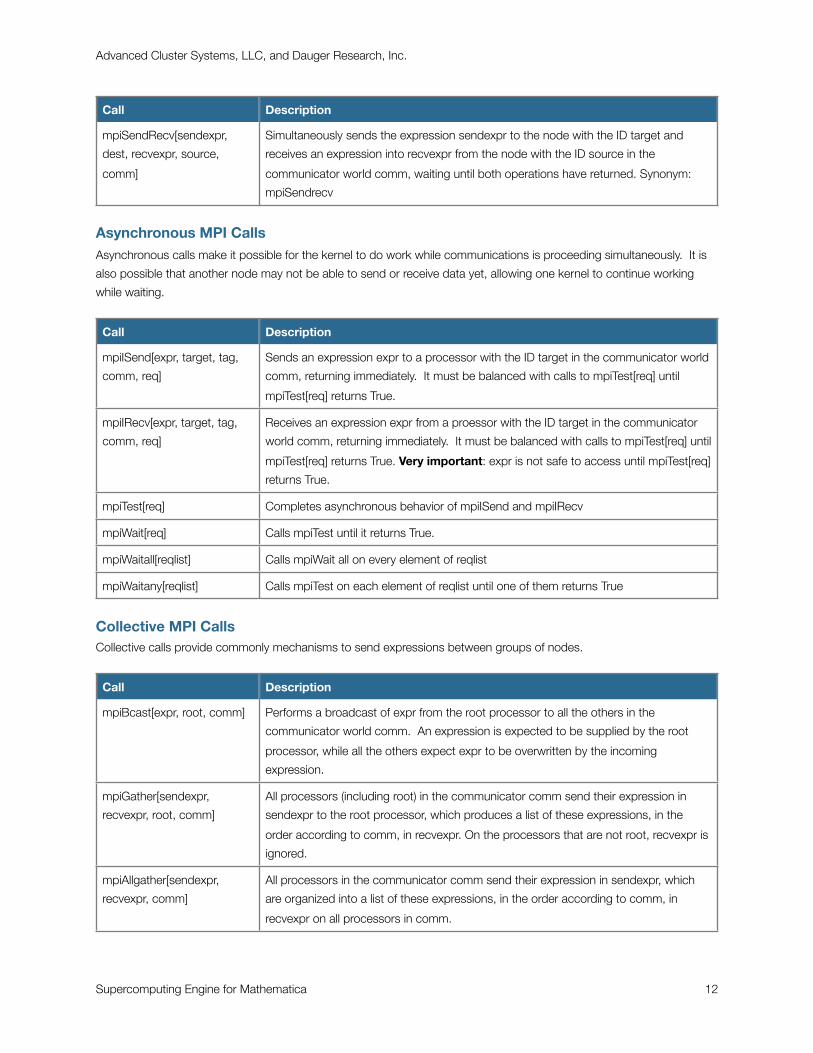
Asynchronous MPI CallsAsynchronous calls make it possible for the kernel to do work while communications is proceeding simultaneously. It is
also possible that another node may not be able to send or receive data yet, allowing one kernel to continue working
while waiting.
Call Description
mpiISend[expr, target, tag,
comm, req]
Sends an expression expr to a processor with the ID target in the communicator world
comm, returning immediately. It must be balanced with calls to mpiTest[req] until
mpiTest[req] returns True.
mpiIRecv[expr, target, tag,
comm, req]
Receives an expression expr from a proessor with the ID target in the communicator
world comm, returning immediately. It must be balanced with calls to mpiTest[req] until
mpiTest[req] returns True. Very important: expr is not safe to access until mpiTest[req]
returns True.
mpiTest[req] Completes asynchronous behavior of mpiISend and mpiIRecv
mpiWait[req] Calls mpiTest until it returns True.
mpiWaitall[reqlist] Calls mpiWait all on every element of reqlist
mpiWaitany[reqlist] Calls mpiTest on each element of reqlist until one of them returns True
Collective MPI CallsCollective calls provide commonly mechanisms to send expressions between groups of nodes.
Call Description
mpiBcast[expr, root, comm] Performs a broadcast of expr from the root processor to all the others in the
communicator world comm. An expression is expected to be supplied by the root
processor, while all the others expect expr to be overwritten by the incoming
expression.
mpiGather[sendexpr,
recvexpr, root, comm]
All processors (including root) in the communicator comm send their expression in
sendexpr to the root processor, which produces a list of these expressions, in the
order according to comm, in recvexpr. On the processors that are not root, recvexpr is
ignored.
mpiAllgather[sendexpr,
recvexpr, comm]
All processors in the communicator comm send their expression in sendexpr, which
are organized into a list of these expressions, in the order according to comm, in
recvexpr on all processors in comm.
Advanced Cluster Systems, LLC, and Dauger Research, Inc.
Supercomputing Engine for Mathematica 12

Call Description
mpiScatter[sendexpr,
recvexpr, root, comm]
Processor root partitions the list in sendexpr into equal parts (if possible) and places
each piece in recvexpr on all the processors (including root) in the communicator world
comm, according the order and size of comm.
mpiAlltoall[sendexpr,
recvexpr, comm]
Each processor sends equal parts of the list in sendexpr to all other processors in the
communicator world comm, which each collects from all other processors are
organizes into the order according to comm.
Additional collective calls perform operations that reduce the data in parallel. The operation argument can be one of the
constants below.
Call Description
mpiReduce[sendexpr,
recvexpr, operation, root,
comm]
Performs a collective reduction operation between expressions on all processors in the
communicator world comm for every element in the list in sendexpr returning the
resulting list in recvexpr on the processor with the ID root.
mpiAllreduce[sendexpr,
recvexpr, operation, comm]
Performs a collective reduction operation between expressions on all processors in the
communicator world comm for every element in the list in sendexpr returning the
resulting list in recvexpr on every processor.
mpiReduceScatter[sendexpr,
recvexpr, operation, comm]
Performs a collective reduction operation between expressions on all processors in the
communicator world comm for every element in the list in sendexpr, partitioning the
resulting list into pieces for each processor’s recvexpr.
Constant Description
mpiSum Specifies that all the elements on different processors be added together in a reduction
call
mpiMax Specifies that the maximum of all the elements on different processors be chosen in a
reduction call
mpiMin Specifies that the minimum of all the elements on different processors be chosen in a
reduction call
MPI Communicator CallsCommunicators organizes groups of nodes into user-defined subsets. The communicator values returned by
mpiCommSplit[] can be used in other MPI calls instead of mpiCommWorld.
Call Description
mpiCommSize[comm] Returns the number of processors within the communicator comm
mpiCommRank[comm] Returns the rank of this processor in the communicator comm
mpiCommDup[comm] Returns a duplicate communicator of the communicator comm
Advanced Cluster Systems, LLC, and Dauger Research, Inc.
Supercomputing Engine for Mathematica 13

Call Description
mpiCommSplit[comm, color,
key]
Creates a new communicator into several disjoint subsets each identified by color.
The sort order within each subset is first by key, second according to the ordering in
the previous communicator. Processors not meant to participate in any new
communicator indicates this by passing the constant mpiUndefined. The
corresponding communicator is returned to each calling processor.
mpiCommMap[comm]
mpiCommMap[comm,
target]
Returns the mapping of the communicator comm to the processor indexed according
to $mpiCommWorld. Adding a second argument returns just the ID of the processor
with the ID target in the communicator comm.
mpiCommFree[comm] Frees the communicator comm
Other MPI Support CallsOther calls that provide other common functions.
Call Description
mpiWtime[] Provides wall-clock time since some fixed time in the past. There is no guarantee that
this time will read the same on all processors.
mpiWtick[] Returns the time resolution of mpiWtime[]
MaxByElement[in] For every nth element of each list of the list in, chooses the maximum according to
Max[], and returns the result as one list. Used in the mpiMax reduction operation.
MinByElement[in] For every nth element of each list of the list in, chooses the minimum according to Min
[], and returns the result as one list. Used in the mpiMin reduction operation.
SetMonitor[state] Sets the MPI monitor window state. 0 means turn off the window and its diagnostics,
1 means open the window (only on Macintosh), and 2 means turn on the window and
write a log of every message to MPIerrs files.
GetMonitor[] Returns the MPI monitor state, as 0, 1, or 2, as described by SetMonitor[].
High-Level SEM CallsBuilt on the MPI calls, below are calls that provide commonly used communication patterns or parallel versions of
Mathematica features. Unless otherwise specified, these are executed in the communicator mpiCommWorld, whose
default is $mpiCommWorld, but can be changed to a valid communicator at run time.
Common Divide-and-Conquer Parallel EvaluationThe following calls address simple parallelization of common tasks.
Call Description
ParallelDo[expr, loopspec] Like Do[] except that it evaluates expr across the cluster, rather than on just one
processor. The rules for how expr is evaluated is specified in loopspec, like in Do[].
Synonyms: SEMDo, SEMParallelDo
Advanced Cluster Systems, LLC, and Dauger Research, Inc.
Supercomputing Engine for Mathematica 14

Call Description
ParallelFunctionToList[f,
count]
ParallelFunctionToList[f,
count, root]
Evaluates the function f[i] from 1 to count, but across the cluster, and returns these
results in a list. The third argument has it gather this list into the processor whose ID is
root.
LoadBalanceFunctionToList
[f, count]
LoadBalanceFunctionToList
[f, count, root]
Like ParallelFunctionToList, evaluates the function f[i] from 1 to count, but across the
cluster, and gathers these results to processor 0 in a list. The difference is that it
performs the functions with load balancing, so that it is less sensitive to different
function calls that take vastly different times to execute. The third argument has it
gather this list into the processor whose ID is root.
ParallelTable[expr, loopspec]
ParallelTable[expr, loopspec,
root]
Like Table[] except that it evaluates expr across the cluster, rather than on just one
processor, returning the locally evalulated portion. The third argument has it gather
this table in to the processor whose ID is root. Synonyms: SEMTable,
SEMParallelTable Exception: If $ParallelTableCollects is set to True, leaving out root
collects results to processor 0.
ParallelFunction[f, inputs,
root]
ParallelFunction[f, inputs]
Like f[inputs] except that it evaluates f on a subset of inputs scattered across the
cluster from processor root and gathered back to root. Without root, the results remain
distributed across processors.
ParallelNIntegrate[expr,
loopspec]
ParallelNIntegrate[expr,
loopspec, digits]
Like NIntegrate[] except that it evaluates a numerical integration of expr over domains
partitioned into the number of processors in the cluster, then returns the sum. The
third argument has each numerical integration execute with at least that many digits of
precision.
Guard-Cell ManagementTypically the space of a problem is divided into partitions. Often, however, neighboring edges of each partition must
interact, so a “guard cell” is inserted on both edges as a substitute for the neighboring data. Thus the space a processor
sees is two elements wider than the actual space for which the processor is responsible. EdgeCell helps maintain these
guard cells.
Call Description
EdgeCell[list] Copies the second element of list to the last element of the left processor and the
second-to-last element of list to the first element of the right processor while
simultaneously receiving the same from its neighbors.
Matrix and Vector ManipulationMatrices are partitioned and stored in processors across the cluster. These calls manipulate these matrices in common
ways.
Advanced Cluster Systems, LLC, and Dauger Research, Inc.
Supercomputing Engine for Mathematica 15

Call Description
ParallelTranspose[matrix] Like Transpose[] except that it transposes matrix that is in fact represented across the
cluster, rather than on just one processor. It returns the portion of the transposed
matrix meant for that processor.
ParallelProduct[matrix,
vector]
Evaluates the product of matrix and vector, as it would on one processor, except that
matrix is represented across the cluster. Synonyms: SEMProduct, SEMParallelProduct
ParallelDimensions[matrix] Like Dimensions[] except that matrix is represented across the cluster, rather than on
just one processor. It returns a list of each dimension.
ParallelTr[matrix] Like Tr[] except that the matrix is represented across the cluster, rather than on just
one processor. It returns the trace of this matrix.
ParallelIdentity[rank] Like Identity[], it generates a new identity matrix, except that the matrix is represented
across the cluster, rather than on just one processor. It returns the portion of the new
matrix for this processor.
ParallelOuter[f, vector1,
vector2]
Like Outer[f, vector1, vector2] except that the answer becomes a matrix represented
across the cluster, rather than on just one processor. It returns the portion of the new
matrix for this processor.
ParallelInverse[matrix] Like Inverse[] except that the matrix is represented across the cluster, rather than on
just one processor. It returns the inverse of the matrix.
Element ManagementBesides the obvious divide-and-conquer approach, a list of elements can also be partitioned in arbitrary ways. This is
useful if elements need to be organized or sorted onto multiple processors. For example particles of a system may drift
out of the space of one processor into another, so their data would need to be redistributed periodically.
Call Description
ElementManage[list, switch] Selects which elements of list will be sent to which processors according to the
function switch[] is evaluated on each element of list. If switch is a function, switch[]
should return the ID of the processor that element should be sent. If switch is an
integer, the call assumes that each elements is itself a list, whose first element is a
number ranging from 0 to the passed argument. This call returns a list of the elements,
from any processor, that is switch selected for this processor.
ElementManage[list] Each element of list must be a list of two elements, the first being the ID of the
processor where the element should be sent, while the second is arbitrary data to
send. This call returns those list elements, from any and all processors, whose first
element is this processors ID in a list. This call is used internally by the two-argument
version of ElementManage[].
Fourier TransformFourier transforms of very large arrays can be difficult to manage, not the least of which is the memory requirements.
Parallelizing the Fourier transform makes it possible to make use of all the memory available on the entire cluster, making
it possible to manipulate problem sizes that no one processor could possibly do alone.
Advanced Cluster Systems, LLC, and Dauger Research, Inc.
Supercomputing Engine for Mathematica 16
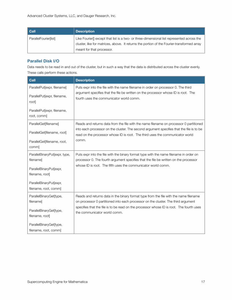
Call Description
ParallelFourier[list] Like Fourier[] except that list is a two- or three-dimensional list represented across the
cluster, like for matrices, above. It returns the portion of the Fourier-transformed array
meant for that processor.
Parallel Disk I/OData needs to be read in and out of the cluster, but in such a way that the data is distributed across the cluster evenly.
These calls perform these actions.
Call Description
ParallelPut[expr, filename]
ParallelPut[expr, filename,
root]
ParallelPut[expr, filename,
root, comm]
Puts expr into the file with the name filename in order on processor 0. The third
argument specifies that the file be written on the processor whose ID is root. The
fourth uses the communicator world comm.
ParallelGet[filename]
ParallelGet[filename, root]
ParallelGet[filename, root,
comm]
Reads and returns data from the file with the name filename on processor 0 partitioned
into each processor on the cluster. The second argument specifies that the file is to be
read on the processor whose ID is root. The third uses the communicator world
comm.
ParallelBinaryPut[expr, type,
filename]
ParallelBinaryPut[expr,
filename, root]
ParallelBinaryPut[expr,
filename, root, comm]
Puts expr into the file with the binary format type with the name filename in order on
processor 0. The fourth argument specifies that the file be written on the processor
whose ID is root. The fifth uses the communicator world comm.
ParallelBinaryGet[type,
filename]
ParallelBinaryGet[type,
filename, root]
ParallelBinaryGet[type,
filename, root, comm]
Reads and returns data in the binary format type from the file with the name filename
on processor 0 partitioned into each processor on the cluster. The third argument
specifies that the file is to be read on the processor whose ID is root. The fourth uses
the communicator world comm.
Advanced Cluster Systems, LLC, and Dauger Research, Inc.
Supercomputing Engine for Mathematica 17

Call Description
ParallelPutPerProcessor
[expr, filename]
ParallelPutPerProcessor
[expr, filename, root]
ParallelPutPerProcessor
[expr, filename, root, comm]
Puts expr into the file with the name filename in order on processor 0, one line per
processor. The third argument specifies that the file be written on the processor whose
ID is root. The fourth uses the communicator world comm.
ParallelGetPerProcessor
[filename]
ParallelGetPerProcessor
[filename, root]
ParallelGetPerProcessor
[filename, root, comm]
Reads and returns data from the file with the name filename on processor 0, one line
for each processor. The second argument specifies that the file is to be read on the
processor whose ID is root. The third uses the communicator world comm.
Advanced Cluster Systems, LLC, and Dauger Research, Inc.
Supercomputing Engine for Mathematica 18

References
Reference materialsTexts used in the creation of this project include descriptions of the MPI standard and guides to parallel computing.
1. M. Snir, S. Otto, S. Huss-Lederman, D. Walker, J. Dongarra, MPI-The Complete Reference, second edition, MIT
Press, Cambridge MA, 1998.
2. G. F. Pfister, In Search of Clusters, Prentice Hall, 1997.
3. V. K. Decyk, “How to Write (Nearly) Portable Fortran Programs for Parallel Computers”, Computers In Physics, 7, p.
418 (1993).
4. V. K. Decyk, “Skeleton PIC Codes for Parallel Computers”, Computers Physics Communications, 87, p. 87 (1995).
For additional informationUseful web sites for learning about parallel computing and techniques to use them are on this site:
http://daugerresearch.com/vault/
It includes links to eight articles on writing parallel code:
• Parallelization - introduces the basic issues when writing parallel code
• Parallel Zoology - compare and contrast the different parallel computing types
• Parallel Knock - exhibition of basic message-passing code
• Parallel Adder - tutorial on parallelizing a single-processor code of independent work
• Parallel Pascal’s Triangle - tutorial on parallelizing propagation-style code requiring local communication
• Parallel Circle Pi - tutorial on creating a load-balancing code divisible into independent work
• Parallel Life - tutorial on parallelizing propagation-style code requiring two-dimensional local communication
• Visualizing Message-Passing - a tutorial on using a graphical monitor window to debug and optimize parallel code
as well as other publications on cluster computing.
Contact informationFor further questions or suggestions email [email protected] and [email protected].
Advanced Cluster Systems, LLC, and Dauger Research, Inc.
Supercomputing Engine for Mathematica 19