Summary ....

Introduction ..

TABLE OF CONTENTSPAGE

· . iii. . 1

Methods 2Current procedure 2

Estimation program 2Estimators 2Outlier detection procedures 2

New procedures 5Standardized Outlier Component Control Charts .. 6Robust Estimator 7

December 1989 Hog Board 8Applications since December 1989 9

Results ....Results for December 1989.Results of September 1989 Simulation

Conclusions ...

Recommendations

References .

Appendix ...

ACKNOWLEDGEMENTS

· .. 10· .. 10· •. 15

. . . . . . . .19

• •• 19

.21

• •• 22

The authors appreciate the initiation of this project by Rich Allenand George Hanuschak. Throughout the project, they providedmanagerial support and encouragement. It was clear they bothstrongly support investigating and establishing formal robustestimation procedures for all multiple frame estimates.

The authors also extend a special thanks to Scot Rumburg for hishelp and investigation of specific outliers observations.

ii

SUMMARYThe National Agricultural statistics service (NASS) conductsquarterly Multiple Frame (MF) hog inventory surveys. The surveydirect expansion estimator for hogs is separated into outlier andnon-outlier components during summary calculations. This reportdocuments a procedure for identifying when the outlier component isunusually large or small. A simple robust estimator that reducesthe impact of unusual outlier components is also presented. TheAgricultural statistics Board used information from theseprocedures when setting the December 1989 hog estimates andrevising September 1989 estimates.

To identify unusual outlier components, standardized outliercomponents (SDOC) are calculated and charted for several quarters.The SDOC gives reviewers a way to judge if the current quarter'soutlier component is influential when compared with previousoutlier components. The robust estimator substitutes the currentquarter's outlier component with an average outlier component overseveral quarters. This discounts the current outlier component andspreads its influence over time. However, the SDOC and the robustestimator can be heavily influenced by unusual historic outliercomponents if not enough historic data are used in thecalculations.

Review of December 1989 robust indications and the Board estimatesindicate that the robust indications influenced Board actions forstates with unusual SDOC's. Simulation of the standardized outliertotals and robust indications for September 1989 indicate that thisinformation would have been helpful to the Board. SDOC controlcharts clearly show the presence of unusual outlier components forseven States in September. The December Board revised the totalhog estimates for five of these seven States in the direction ofthe robust indication. These revisions probably would have beenreduced or eliminated if the SDOC's and robust indications had beenavailable in September.

Clearly these procedures provided useful information to theDecember 1989 Hog Board. Currently, only the robust indication issupplied for the 10 State, 16 State and U.S. total hog estimates.No State level robust indications are used and no standardizedoutlier charts are used at any level.

NASS research and operational statistical methodology units shouldput high priority on jointly developing and implementing robustmultiple frame procedures. Based on this review and evaluation ofthe procedures used for the December 1989 Hog Board, we recommendthe following:

iii

1. Examine methods that reduce the impact of unusualhistoric outlier components on the SDOC and robust estimator. Thisshould include reviewing the amount of historic data used forcalculating the SDOC and robust indications.

2. Review present outlier cutoff limits and examine othercriteria for determin ing these cutoff 1imits. Current cutofflimits do not provide meaningful outlier components for manystates.

3. Research staff should study the statisticalcharacteristics of individual outliers and other components to aidin the development of effective outlier detection and robustestimation procedures.

4. Modify the operational summary systems with several newexperimental outlier cutoff limits and store individual outlierobservations for robust estimation analysis and review.

Once 1 through 4 have been resolved then:

5. The Agency should make it an important goal to implementoutlier detection and robust estimation techniques for SSO andNational Board reviews of most MF crop and livestock estimates.

iv

A Review and Evaluation of Unusual Outlier Component Detectionand Robust Estimation Procedures used by the

December 1989 Hog BoardGary Keough and Charles R. Perry, Jr.

INTRODUCTIONoutliers are common in agricultural commodity survey data becausepopulations are often highly skewed with a large number of smallvalues and a few very large values. However, limited attention isgiven to outliers until they dominate the estimator. Thomas,Perry, and Viroonsri4 examined Empirical Bayes and right censoredestimators for highly skewed populations in order to dampen outliereffects. This report documents procedures to identify when theoutlier component in repeated survey data are unusually larger orsmaller than expected, and a simple robust estimator to be usedwhen this occurs. Dr. Charles Perry developed these procedures forthe National Agricultural statistics Service (NASS) December 1989Hog Board. The Chairperson of the Agricultural Statistics Board,Rich Allen, felt outliers overly influenced the September 1989 hogdata and a procedure for dampening their effect was needed. Sinceoutl ier observations frequently occur in successive NASSAgricultural Surveys within a survey year (June-March) due tosample design, numerous outliers were expected in the December 1989survey.

For this report, an outlier will be broadly defined as an expandedvalue considered unusual or influential by some defined procedure.The outlier component is the sum of these expanded values.

1

Metho~sCurrent proce~ures

Estimation proqram

NASS has estimated quarterly hog numbers in the 10 maj or hogproducing states since 1975. These states are Georgia, Illinois,Indiana, Iowa, Kansas, Minnesota, Missouri, Nebraska, NorthCarolina, and Ohio. In 1988 NASS started making quarterlyestimates for the 16 major hog producing states by adding Kentucky,Michigan, Pennsylvania, South Dakota, Tennessee, and Wisconsin.These 16 States produce about 90 percent of the u.s. total hogs.Only annual estimates as of December 1 are made for the remainingstates.

Estimators

NASS uses a multiple frame (MF) approach for estimating maj oragricultural commodities from the Agricultural Survey Program(ASP). This approach utilizes a list frame and an area frame forproviding survey indications. The list frame consists of a list offarming operations and associated control data. Control data areused to stratify the list frame to improve sampling efficiency. Amajor disadvantage of almost any list frame is that it seldomcontains the entire population of interest. The NASS area frame iscomplete and allows any area of land in the continuous 48 States tobe selected with a known probability. Consequently, the area frameis used to account for the list frame's incompleteness in the MFapproach.Each reporting unit in the area frame sample is matched against thelist frame to determine whether it is on the list or not.Reporting units not on the list frame represent the nonoverlap(NOL) population. The MF estimator is the sum of the list and NOLcomponents. The NOL component is the main contributor to thevariance of the estimator. Outliers typically come from smalloperation list strata and the NOL domain. These have smallsampling fractions and therefore have large expansion factors.For a more detailed discussion of NASS's multiple frame approachsee Nealon2 or Thomas et al.4

A second MF indication adjusts the MF direct expansion (DE) fornonresponse based on information about presence or absence of hogsfor the nonrespondents'. Any outliers that affect the original MFDE would also affect the adjusted indication.

outlier detection procedures

NASS uses two different procedures in the current hog summary andanalysis system for detecting outliers. Each procedure isdescribed below.

2

The oldest procedure, Procedure 1, uses fixed state level cutoffvalues to identify if an observation's expanded value is anoutlier. Table 1 gives the cutoffs by state in 1,000's. Thisprocedure is used on both the LIST and NOL components of themultiple frame data. The history of Procedure 1 is obscure. Nohistorical documentation describing its development is available.The procedure has been a part of NASS's Enumera-tive Summary Systemsince its implementation in 1977.

TABLE 1 -- Procedure 1 cutoff values in l,OOO's of hogs

16 major hog States

GeorgiaIllinoisIndianaIowa

25504080

KansasMinnesotaMissouriNebraska

20404040

N. Carolina 30Ohio 25Kentucky 20Michigan 15

Pennsylvania20S. Dakota 25Tennessee 20Wisconsin 25

Remaining 32 States

Alabama 10Arizona 5Arkansas 10California 5Colorado 10Connecticut 5Delaware 5Florida 10

Idaho 5Loui sLma 5Maine 3Maryland 5Massachusetts 5Mississippi 10Montana 5Nevada 4

N. Hampshire 3N. ,Jersey 5N. Mexico 5N. York 5N. Dakota 5Oklahoma 15Oregon 5Rhode Island 3

S. Carolina 10Texas 20Utah 5Vermont 3Virginia 15Washington 5W. virginia 5Wyoming 5

It appears the state cutoffs are set at approxirrately one percent ofstate's historical hog inventory. Except for the addition of somesmaller states, cutoff limits have the not changed since 1977.

The average percent of the ~F DE due to the outlier component wascalculated using 1975 to 1989 quarterly information for the 10 majorhog States. Average percentages for the remainder of States werecalculated using 1988 and 1989 information. Figure 1 shows theoutlier component is typically 5 to 10 percent of the MF DE for the10 major hog states and about 6 percent at the 48 state level. Theaverage percent varies more among the remaining states. Some Stateshave had outlier components averaging over 45 percent of the MF DEfor these 2 years. Nine states have averaged over 25 percent.

Cutoff limits should be reviewed to insure tha~ meaningful outliercomponents are provided. Outlier components that are 40 percent ormore of the estimate are hardly useful or meaningful. However, itmay not be possible to provide consistently meaningful cutoff limitsfor the very small states with just a few positive reports since anyof these reports can have a large influence on the total DE. Thomaset al.4 discuss cutoff limits in terms of upper quantiles.

3

Figure 1. Outlier Component as a Percentof the Direct Expansion

State/Region

o 5 10 15 20 25 30 35 40 45 50

Percent10 Major States' percents calculatedfrom 1975-1989 Quarterly data, otherscalculated from 1988-1989 Quarterly data

4

The historical NASS database contains state level outliercomponents and standard deviations from all observations classifiedas outliers by this procedure, but neither the individual outliersnor the number of outliers have been archived .. Quarterly statelevel outlier components and standard deviations are available forthe 10 major hog producing States starting with the December 1975quarter. All other States start with the March 1988 quarter.

The newer procedure, Procedure 2, uses historical stratum variancesto detect influential list observations at the stratum level.Procedure 2 was implemented in 1982.5 This procedure compares eachobservation's value to the stratum mean. List values larger than10 standard deviations from the stratum mean are classified asoutliers. This procedure's outlier component was about 3.5 percentof the National estimate in June 1989 and about 4 percent inSeptember 1989.

Two censored estimates that adjust for outliers are computed fromProcedure 2. The first excludes outlier observations and treatsthem as inaccessible responses. The summary system adjusts thesample count of usable observations used to calculate the stratumexpansion factors. The second also excludes outlier observationsbut treats them as positive inaccessible responses in thenonresponse adjustment procedure.

The historical NASS database does not contain individualobservations or the summary statistics from this procedure.However, the list frame individual outliers are available for allquarterly surveys starting with the December 1988 quarter inspecial databases managE~d by statistical Methods Branch. Thecensored estimates are also available starting with the June 1989quarter. Several additional quarters of censored estimates frommicrofilm copies of the hog analysis package output could berecovered with a sufficient clerical effort.

It should be noted that Procedure 2 involves only the list frameand therefore gives no indication of outliers in the NOL componentof the multiple frame estimates. Because the NOL accounts forbetween 2/3 to 3/4 of the total variance in the hog series andbecause of limited data, no further analyses using Procedure 2 datawas justified.

New ProceduresThe techniques described below were produced using Procedure 1historical data. They are intended to supplement currentindications used by the Agricultural Statistics Board in settingNational, Regional and state hog estimates.

The techniques can be divided into two logical groups for ease ofdiscussion;

5

1. Standardized outlier component control charts for thedetecting unusual outlier components, and

2. A simple robust procedure which will dampen the effect ofunusual outlier components.

These procedures are based on the assumption that an averageoutlier component is expected each survey. It is recognized thata sample is not perfect and the outlier component from a sample maynot truly represent the population. The new procedures aredesigned to identify when unusually large or small outliercomponent occur and dampen their affect on the survey expansion.

standardized Outlier Component Control Charts

standardized outlier component (SDOC) control charts identify whenthe current outlier component is unusual compared to previousoutlier components. The SDOC for quarter t, SDOC

t, is calculated

as:

where

0t the outlier component for quarter ti

is the mean of the historic outlier components;

is the standard deviation of the historic outliercomponents;

and n, = the number of quarters from t=l to t-l.

The quarters 1 through n, make up a sliding window. Each quarter,the previous n, quarter's outlier components make up the historicbase used to calculate SDOC's.

For general guidelines to interpret SDOC control charts, considerthe standardized normal distribution, a normal distribution withmean zero and variance of one. Typically, any observation from astandardized normal distribution with a value greater than two orless than minus two is considered unusual. The SDOC values can beinterpreted similarly. This is a generalization and does not implywe can assign probabilities to the event a SDOC is larger than a

6

given value. However, as the SDOC gets larger in absolute value,the more unusual the outlier component is compared to historicoutlier components. We can consider SDOC's within plus or minustwo as common. However, when SDOC's are beyond plus or minus twothe outlier component is influencing the MF DE and moreconsideration should be given to the robust estimator.

Note the outlier component for the current. quarter is not used tocalculate the historic outlier component mean and standarddeviation. Consequently, the current quarter SDOC is anindependent comparison of the current outlier component against itshistoric base. The SDOC is not an indication of the size of theoutlier component. Also, SDOC's, as defined here, are to berecalculated each quarter because each current quarter has adifferent historic base.

Robust Estimator

When an unusually large or small outlier component occurs, the MFwill provide an unreliable indication of the population total.Recall that an underlying assumption of this robust approach isthat it is possible for an unusual outlier component to occur onany survey but its value may not be representative of the trueoutlier component. A better estimate is an average which spreadsunusual outl ier levels over several surveys. Thomas et al.4

examined an empirical Bayes method to stabilize the current surveyestimate. A right-censored estimator for the NOL component of theMF estimate was also examined. The robust estimator presented hereis similar to the right-censored estimator but is applied to theNOL and list components of the sample. The robust estimatorintroduced to the December 1989 Hog Board smooths out the currentquarter's outlier component's influence by replacing it with theaverage outlier component from several quarters. The main reasonfor using the procedure is it's simplicity. The robust estimatorfor quarter t, Rt' is calculated as:

R t = X t - °t + 0h2; ( 1)

where

Xt indication for quarter of interest,

0t = the outlier component for quarter of interest,

is the mean outlier component, and

nz = n, plus the curent quarter.

7

Notice the robust estimator uses all outlier components incalculating the mean outlier component. This procedure spreads anunusual outlier component's influence out over several quarters sothat it does not dominate the current quarter's indication.

The number of quarters, n2, is presently a subjective choice.Guidelines for choosing the number of quarters should be examined.If n2 is too small, influential outlier components are not spreadover enough quarters, possibly causing the robust estimator to bebiased. Similarly, if n2 is too large, any trend in the size ofthe outlier component may also cause the robust estimator to bebiased.

December 1989 Hog BoardFor the December 1989 Hog Board, the robust estimator was appliedto the MF DE and the adjusted MF DE indications. SDOC'controlcharts and time series charts showing the relationship of the MFDE, adjusted MF DE, robust DE, adjusted robust DE, MF DE minusoutlier component, adjusted MF DE minus outlier component, andoutlier component were provided. Time series charts and additionalcomputer listings displayed warning messages when the SDOC was 2 orlarger. Charts and listings were generated for the individual 48multiple frame States, the 16 State Region, 32 State Region, and 48State Region.

SDOC's and robust indications were calculated using outliercomponents from the March 1988 through December 1989 quarters.This corresponds to the start of MF estimates for 48 continuousstates. This was done for convenience since data prior to March1988 is not available for all States. The standardized outliercomponent for December 1989, SDOCo~' was calculated as:

SDOCV89 = (OV89 - 0hl) / So

where

0089 = outlier component for December 1989,

0h1 = mean outlier component calculated using outlier totalsfrom March 1988 through September 1989,

So standard deviation calculated using outlier totals fromMarch 1988 through September 1989.

The robust indications were calculated as:

where

8

= the MF DE when i=l,the adjusted MF DE when i=2,

= mean outlier component calculated using outliercomponents from March 1988 through December 1989.

Note that March 1988 through September 1989estimated using the 6hZ• Thus, robustquarters are calculated using one orcomponents. This was done because of theavailable. In an operational setting,components would be used.

robust indications wereindications for thesemore future outlier

limited amount of dataonly previous outlier

Applications since December 1989currently, only U.S., 10 State, and 16 State Regional chartsshowing the robust indications and Board estimates are provided tothe Board. These charts show March 1988 to present quarterindications. Robust indications are calculated using the March1988 to present outlier components. No state level time seriescharts are used and no SDOC control charts are used at any level bythe Board.

9

RESULTS

Results will be presented in two sections. The first sectiondocuments materials provided to the December 1989 Hog Board. Thesecond section presents an analysis of the September 1989 surveywith SDOC's and robust indications.

Results for December 1989

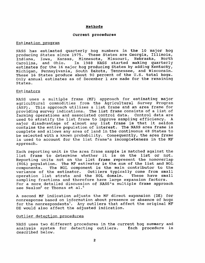
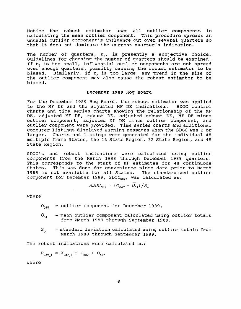
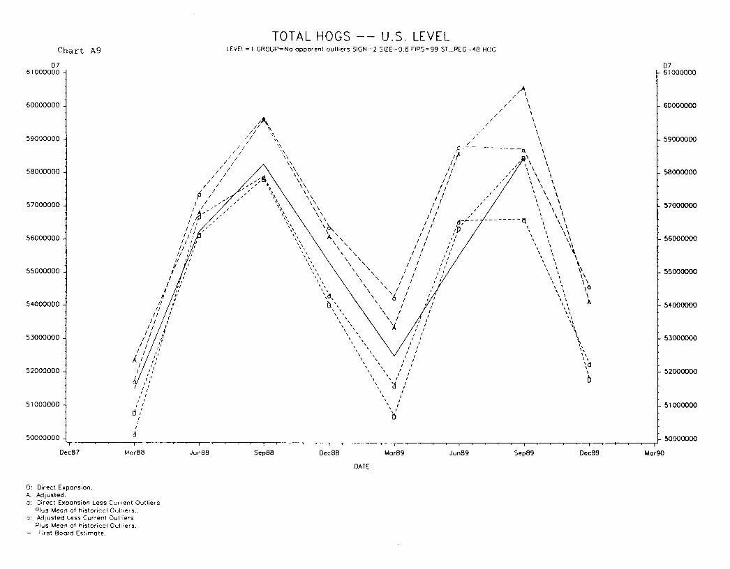
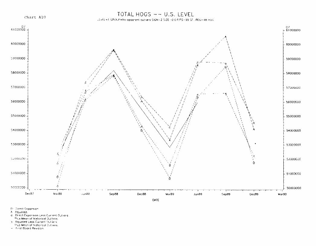
Charts A1 through All in the Appendix are copies of 48 State regionmaterial provided the December 1989 Hog Board. Charts A1 throughA8 show different combinations of the Multiple frame indications,Multiple frame indications minus outlier components, robustindications, first Board estimates, first Board revisions, and theoutlier component. Chart A9 shows only the indications from ChartA3 on a different scale. Chart All is a SDOC control chart.Figures 2-4 are reproductions of the SDOC control charts for the 48State region, 10 State region, and Georgia.

Figures 2 and 3 show that the December SDOC is about -0.5. Thisimplies the December outlier components are not unusual compared tothe previous seven quarters. Figure 4 shows Georgia's SDOC forDecember was about 3.5. This indicates the Georgia's robustindications should be followed more closely than the MF DE andadjusted MF DE. The large December SDOC is due to one NOLoperation that expanded to about 714,000 head in December, or about60 percent of the state's total.

Figure 2. SDOC Control ChartU.S. level, December 1989

41--------~- -~--~~~~~---------------I3.5 r

3LI

2.~ ~ i1.5 ,/ " I

1 \ i\

0.5 \

-o.~ ~.-~~-_~- 1 I

- 1.5 f--2i

Mar Jun Sep1988

Dee Mar Jun Sep1989

DeeI

Standardized Outlier

10

Figure 3. SDOC Control Chart,10 State level, December 1989

I

IIi1

DeeI

- Standardized Outlier

Figure 4. SDOC Control Chart,Georgia, December 1989

4 ,--------

3.5 ~3 '

2.52

1.51

0.5o ---~-

-0.5 _-~---------~---

- 1- 1.5.

_2 L I ~ --' -~-- ---- - _J

Mar Jun Sep Dee MarI 1988

//

- ~---------j

II

-~--~-----~

Jun Sep Dee1989 1

- Standardized Outlier

11

Table 2 shows the SDOC's for the 10 state, 16 state, 32 state, 48state Region, and the 16 individual states from the December 1989Survey. Besides the unusually large SDOC for Georgia, unusuallysmall outlier components for Minnesota and the 32 state Region arepresent. Although Table 2 alone would identify potential outlierproblems, review of the control charts is recommended to identifyany long term problems or trends. For instance, Figure 4 showsthat Georgia's outlier component had been fairly constant untilMarch 1989 then it substantially increased in June, september, andDecember. This information should help with post-survey analysisand revisions. It is also noteworthy that the Regional SDOC's showno apparent outlier problems, but unusual SDOC's could exist forindividual states. In the December 1989 survey, Georgia andMinnesota help offset each other so that the 10 State and 16 Stateregional SDOC's are small. It is important to review eachpublished state's control chart.

Recognizing the unusual outlier levels for Georgia, Minnesota, andthe 32 State Region, Figures 5,6,7, show how the Board used thesimple robust indications in these situations. For Georgia, theDecember MF DE and adjusted MF DE are biased upward due to outliersso the Board more closely followed the robust indications. ForMinnesota and the 32 State Region the MF DE and adjusted MF DE arebiased downward due to small outlier levels, so the Board moreclosely followed the higher levels indicated by the robustindications. In all three cases, apparently the robust indicationswere influential on the Board estimate. Table Al (in the Appendix)shows the indications, first Board and revised estimates, anddifferences for all 16 States and the regions.

Additional review of Figure 5 illustrates the problem of notspreading influential outlier components over enough quarters.Note that the March 1988 through March 1989 robust DE and adjustedrobust DE are substantially higher than the MF DE, adjusted MF DE,and Board values. This is because the large September and Decemberoutlier components are included in the average outlier component.Recall equation 1,

Rt = Xt - 0t + 0h2·

If the average outlier component (Oh2) is substantially larger thanthe current outlier component (Ot)' the robust indication will besubstantially larger than the DE. The intent of the estimator isthat this average will be a "better" indication of the true outliercomponent level. However, the average used in Figure 5 includesthe large September and December outlier component values.Consequently, averages and robust estimates are probably biasedupward for all quarters. This is most noticeable in March 1988through March 1989 where the original outlier component wasrelatively small. This impact could possibly be reduced byincreasing the number of quarters used to calculate 0hZ. Althoughthis is an artificial setting since future data are used to

12

calculate the average outlier component, it still shows largeoutlier components in previous quarters have a major impact on theaverage outlier component if it is calculated with too fewquarters.

Figure 5. Total Hogs--GeorgiaDecember 1989

Thousands1700

1600

1000Mar

IJun Sep

'988Dee Mar JUIl Sep

'989Dee

I

-- D.E. -+--- Adj.D.E. -- Board -+- Ro.D.E. --b- Ro.A.D.E.

13

Figure 6. Total Hogs--MinnesotaDecember 1989

Thousands540052005000

48004600440042001

4000 LMar

I

Jun Sep1988

Dee Mar Jun Sep1989

DeeI

- ,j:-- D.E. -B- Adj.D.E. --+- Board --4- Ro.D.E. --A- Ro.A.D.E.

Figure 7. Total Hogs--32 StateDecember 1989

Thousands540052005000480046004400 7

4200400038003600Mar

IJun Sep

1988Dee Mar Jun Sep

1989Dee

I

--- D.E. -B- Adj.D.E. -- Board --4- Ro.D.E. --A- Ro.A.D.E.

14

Table 2 -- SDOC's for December 1989 Multiple Frame Survey by State

Standardized Standardized Standardized StandardizedOutlier Outlier Outliers Outlier

State Totals State Totals State Totals state Totals

GA. 3.5 KANSAS -0.4 N.CAR. -1.2 PA. 0.3ILL. -1.1 MINN. -2.0 OHIO -1.4 S.DAK. 1.0IND. 0.3 MO. -1.0 KY. 0.4 TENN. -1.6IOWA. -1. 5 NEB. 1.2 MICH. 0.5 WISC. 1.6

10 HOG -0.4 16 HOG -0.2 32 HOG -2.0 48 HOG -0.6

Results of September 1989 simulationDuring the September 1989 survey, it was recognized that outlierswere greatly affecting the survey indications. Analysis wasconducted to examine the possible impact of the outlier detectionand robust estimation techniques if they had been available. To dothis the SDOC's and robust indications were recalculated as if inan operational setting. That is, each charted robust indicationwas calculated using only previous survey data. The SDOC valuesfor the original 10 major hog States were calculated using theprevious seven quarters' (December 1987-June 1989) outliercomponents, while the previous six quarters (March 1988-June 1989)outlier components were used for the remaining six States. Thissimulation is only an example of many possible approaches. Thisapproach was chosen to mirror the December 1989 procedures as muchas possible.

Figure 8 is an example of a simulated September 1989 time serieschart using Georgia hogs indications. Figure 9 is the SDOC controlchart. These figures are similar to Charts A5 and A6,respectively.

Figure 8 shows the robust indications support the Board estimatesup through June 1989. The large September outlier component causesthe MF survey indications to increase over 200,000 hogs from theJune indications while the robust indications decline slightly.Figure 9 shows Georgia's September SDOC is about 8, extremelyunusual. Figures 8 and 9 clearly show the Septe~ber 1989 outliercomponent in Georgia was unusually large and affected the multipleframe indications.

15

",. I,¥/1000 _~._]' 1_.

Dee Mar Jun Sep Dee Mar Jun Sep Dee Mar Jun Sep1986 i 1987 1988 1989 I

Figure 8. Total Hogs--GeorgiaSeptember 1989

Thousands1600

1500

1400

1300

1200 .

1100

---+-- D.E. -+- Adj.D.E. --><- Board -4- Ro.D.E. --b--- Ro.A.D.E.

Figure 9. SDOC Control Chart,Georgia, September 1989

oard

87

6

5

4

321

o- 1

-2Dee19B7

Mar Jun Sep1988

Dee Mar Jun1989

SepI

- Standardized Outlier

16

Comparing Figure 9 (Georgia's September SDOC control chart) withFigure 4 (Georgia's December SDOC control chart) illustrates theimpact that an unusually large outlier component can have on SDOCvalues. Georgia's September outlier component was 598,574. TheSeptember chart (Figure 9) shows this value had a SDOC of abouteight while the December chart (Figure 4) shows September with aSDOC of about two. This is because a different historic base isused each month to calculate the historic outlier component average«\,) and standard deviation (So). September's large outliercomponent is not used to calculate Figure 9's SDOC's while it isused to calculate Figure 4's SDOC' s. This also shows that oneprevious quarter's large outlier component can have a major impacton the current quarter's SDOC if it is calculated with too fewquarters of data. Table 3 shows the historic mean and standarddeviations are very different for each chart. This demonstratesthat the current quarter SDOC is simply a comparison of the currentquarter outlier component against its historic base. It does notindicate the actual size of the outlier component.

Table 3 -- Comparison of Georgia's SDOC values

eptemberSDOCValue 1/

Historic September SSDOC Historic standard OutlierChart Mean Deviation Component

September 127,398 585,810 598,574

December 192,323 188,331 598,574

8

2

1/ SDOC September Outlier Component-Historic M~anHistoric Standard Deviation

Table 4 shows six States, Georgia, Indiana, Minnesota, Nebraska,Ohio, and Wisconsin would have had SDOC's greater than two. TheSDOC for N. Carolina would have been -2.7. Also the, 10 StateRegion, 16 State Region, and National levels would have hadsimilarly high SDOC's. It is obvious there were several unusualoutlier components in the September data.

Table 4 simulated standardized outlier components for September 1989Multiple Frame Survey by State

State SDOC State SDOC State SDOC State SDOC

GA. 8.0 KANSAS -1.9 N.CAR. -2.7 PA. 1.1ILL. 0.6 MINN. 3.5 OHIO 3.4 S.DAK. -0.2IND. 3.0 MO. -1.2 KY. 0.5 TENN. -1.1IOWA. -0.6 NEB. 3.4 MICH. -0.3 WISC. 3.2

10 HOG 3.4 16 HOG 4.4 32 HOG 1.3 48 HOG 3.3

17

Recognizing the impact that the SDOC charts and robust indicationshad on the December Board estimates, it is probable that theSeptember estimates would have been similarly affected. Estimatesfor states with large SDOC's (larger than two) would have followedthe lower robust indications more closely than the operational MFindication. Estimates for States with small SDOC's (smaller thanminus two) would have followed the larger robust indication moreclosely. The initial Board estimates for these targeted states andRegions were subsequently revised as indicated in Table 5. Ingeneral, these revisions were in the direction anticipated by theSDOC value and robust indication. Only North Carolina and ohiowere not revised. Quite likely, revisions would not have beennecessary or at least reduced if these procedures had beenavailable in September.

Table 5 -- September 1989 Hog Indications and Board Estimate

simulated MF Robust First Revisedstate SDOC DE DE Board Board

GA. 8.0 1482 1070 1300 1250IND. 3.0 5158 4440 4650 4550MINN. 3.5 5036 4802 5050 4950NEB. 3.4 4424 4132 4450 4350N.CAR. -2.7 2627 2780 2700 2700OHIO 3.4 2277 2125 2300 2300WISC. 3.2 1407 1239 1350 1300

10 HOG 3.4 45927 44511 45800 4520016 HOG 4.4 53199 51526 53045 52395

Table A2 shows the indications, first Board and revised estimates,and differences for all states and Regions.

18

CONCLUSIONSOccasionally and unpredictably, outliers have a large impact onstate, Regional, and National survey indications. Techniques areneeded to identify when unusual outliers occur and to providerobust indications that dampen the effect of the outliers. Aftera thorough review of outlier detection and robust techniques,simple procedures were developed and implemented for the December1989 Hog Board. SDOC control charts clearly identified thatunusually large and small outlier components were present for somestates and Regions in the December 1989 data. Review of theOfficial estimates indicate that the robust indications didinfluence the Board action for these states and Regions. Analysisalso indicates that SDOC control charts would have identifiedunusual outlier components in the September 1989 data and thatusing the robust indications could have reduced or eliminated therevisions that were later necessary. However, unusual outliercomponents will have a large impact on the SDOC and robustestimator if not enough historic data are used. Also, currentoutlier cutoff limits are not meaningful for many States.

RECOMMENDATIONSNASS research and operational statistical methodology units shouldput high priority on jointly developing and implementing morerobust multiple frame procedures. After reviewing how the SDOCcontrol charts and the robust estimator performed for the December1989 Hog Board and in the September 1989 simJlation, we recommendthe following:

1. Examine methods that reduce the impact of unusual historicoutlier components on the SDOC and robust estimator. This shouldinclude reviewing the amount of historic data used for calculatingthe SDOC and robust indications.

2. Review present outlier cutoff limits and examine othercriteria for determin ing these cutoff Iim its. Current cutoffIimits do not prov ide meaningful outl ier components for manystates.

3. Research staff should study the statistical characteristicsof individual outliers and other components to aid in thedevelopment of effective outlier detection and robust estimationprocedures.

4. Modi fy the operational summary systems with several newexperimental outlier cutoff limits and store individual outlierobservations for robust estimation analysis and review.

Once 1 through 4 have been resolved then:

19

5. The Agency should make it an important goal to implementoutlier detection and robust estimation techniques for SSO andNational Board reviews of most MF crop and livestock estimates.

20

REFERENCES1. Crank, Keith N., The Use of Current Partial Information toAdiust for Non Respondents. April 1979, USDA, ESCS, SRD.

2. Nealon, Jack P., Review of the Multiple and Area FrameEstimators, USDA, SRS, SF & SRB Staff Report No. 80, March 1984.

3. Perry, Charles R., Short Term Technical Assistance Trip ReportAnal ysis and Evaluation of Cameroon Aqricul t,ural Survey Desiqn.Final Report, U.S. Dept. Agr., Nat. Agric. stat. Serv., May 15,1990.

4. Thomas, David R., Perry, Charles R., viroonsri, Boonchai,.Estimation of Totals for Skewed Populations in RepeatedAqricul tural Surveys Hoqs and piqs. NASS Research Report No.SRB-90-02. U.S. Dept. Agr., Nat. Agric. Stat. Serv., April 1990.

5. U.S. Department of Agriculture, National Agriculturalstatistics Service. Iechnical Directive T-49-82.

6. U.S. Department of Agriculture, statistical Reporting Service.Scope and Methods of the statistical Reportinq Service. Misc. Publ.No. 1308, September 1983.

21

APPENDIXTable A1 -- Multiple frame and robust indications, first and revised Boardestimates, 16 major hog states, December 1989

Multiple Frame Ind. Robust Ind. Board

Adj. Adj.state DE *diff DE *diff DE *diff DE *diff First *diff Revised

(000)GA. 1670 -470 1687 -487 1086 114 1103 97 1200 0 1200ILL. 5307 393 5696 4 5460 240 5849 -149 5700 0 5700IND. 4307 43 4489 -139 4196 154 4379 -29 4350 0 4350IOWA. 13022 478 13481 19 13500 0 13959 -459 13500 0 13500KANSAS 1367 83 1461 -11 1378 72 1472 -22 1450 0 1450MINN. 4062 388 4369 81 4262 188 4569 -119 4450 0 4450MO. 2539 161 2612 88 2598 102 2672 28 2700 0 2700NEB. 3793 407 4131 69 3628 572 3966 234 4200 0 4200N.CAR. 2564 6 2651 -81 2664 -94 2751 -181 2570 0 2570OHIO 1807 273 1916 164 1906 174 2015 65 2080 0 208010 HOG 40437 1763 42492 -292 40680 1520 42735 -535 42200 0 42200

KY. 961 14 990 -15 940 35 968 7 975 0 975MICH. 1247 13 1282 -22 1224 36 1258 2 1260 0 1260PA. 940 35 955 20 926 49 941 34 975 0 975S.DAK. 1754 -34 1862 -142 1709 11 1817 -97 1720 0 1720TENN. 653 47 671 29 795 -95 813 -113 700 0 700WISC. 1298 -48 1329 -79 1166 84 1197 53 1250 0 125016 HOG 47289 1791 49579 -499 47438 1642 49728 -648 49080 0 4908032 HOG 4526 246 4573 199 4840 -68 4886 -114 4772 0 4772US HOG 51816 2036 54152 -300 52278 1574 54615 -763 53852 0 53852

*diff is the Revised Board Estimate minus the previous indication.

22

Table A2 -- Multiple frame and simulated robust indications, first andrevised Board estimates, 16 major hog states, September 1989

Multiple Frame Ind. Simulated Robust Ind. BoardAdj. Adj.

State DE *diff DE *diff DE *diff DE *diff First *diff Revised-

(000)GA. 1482 -232 1504 -254 1070 180 1092 15 1300 -50 1250ILL. 5951 149 6181 -81 5879 221 6108 -8 6100 0 6100IND. 5158 -608 5289 -739 4440 110 4571 -21 4650 -100 4550IOWA. 14635 -35 15208 -608 14816 -216 15389 -789 14800 -200 14600KANSAS 1536 14 1639 -89 1579 -29 1682 -132 1600 -50 1550MINN. 5036 -86 5341 -391 4802 148 5108 -158 5050 -100 4950MO. 2801 49 2854 -4 2889 -39 2942 -92 2850 0 2850NEB. 4424 -74 4708 -358 4132 218 4415 -65 4450 -100 4350N.CAR. 2627 73 2676 24 2780 -80 2829 -129 2700 0 2700OHIO 2277 23 2363 -63 2125 175 2211 89 2300 0 230010 HOG 45927 -727 47764 -2564 44511 689 46348 -1148 45800 -600 45200KY. 1028 -3 1047 -22 998 27 1017 8 1025 0 1025MICH. 1262 38 1315 -15 1277 23 1330 -30 1300 0 1300PA. 1038 -18 1045 -25 982 38 989 31 1020 0 1020S.DAK. 1756 -6 1860 -110 1767 -17 1871 -121 1750 0 1750TENN. 781 19 813 -13 874 -74 906 -106 800 0 800WISC. 1407 -107 1429 -129 1239 61 1261 39 1350 -50 130016 HOG 53199 -804 55273 -2878 51526 869 53600 -1205 53045 -650 5239532 HOG 5280 -80 5320 -120 5400 -200 5078 122 5114 86 5200US HOG 58479 -884 60594 -2999 58445 -850 56687 908 58601 -1006 57595

--. --

*diff is the Revised Board Estimate minus the previous indication.

23

Chart Al

D770000000

TOTAL HOGS -- U.S. LEVELLEVEL=1 GROUP=No opporent outliers SIGN=2 512E=0.6 FIPS=99 ST_REG=48 HOG

D770000000

50000000

50000000

40000000

.30000000

20000000

10000000

o

o

o

_---f<:-- _

o o o

__ .....-/1\-

_---0-- -- - -----0""' _

_-d-------------~--_

o

o o

60000000

50000000

40000000

.30000000

20000000

10000000

oDee87 Mor88 Jun88 Sep88 Dee88

DATE

Mor89 Jun89 Sep89 Dec89 Mar90

D: Direct Expansion.". ~dJusted.d: Direct Expansion Less Curre~t OutlIers.a: ~dJusted Less Current OutlIers.-' F:rst Boord ~stimote.o Sum of 011 Outliers.

Chart A2

0770000000

60000000

50000000

40000000

30000000

2COOOOOO 1j

10000000

TOTAL HOGS -- U.S. LEVEL

a

0770000000

60000000"- "- "- "-

;a.

n50000000

1:J

d

40000000

30000000

20000000

'0000000

a a a o

c.--~~----'---r--~-~~..-----,---~'----, --,-_~-~- ~~_~~_~_~ ~__~M,,, fOR

oDec8? Jun88 Sep88 Dec88 Mor89 Jun89 Sep89 Dec89 Mar90

o

DATE

D: Direct Expansion.'" Adjusted.j. Dlr~ct Expon310n Less Current Outl'ersJ Adjusted Less Current Cut llers

r;rst Boord Revt~'on) SuM of all Outliers.

Chart A3

077COOOOOO

60000000

50000000

40000000

30000000

20000000

TOTAL HOGS -- U.S. LEVELLEVEL=l GROUP=No apparent outliers SIGN=2 SIZE=O 6 FIPS=99 ST_REG=48 HOG

0770000000

60000000

50000000

40000000

30000000

20000000

10000000

aa

<J 0 0 aa

0

0~cB7 ~orBB JunBB S~p88 O~cBB ~orB9 Jun89 S~p89

OATE

D. Dir~ct Expansion.k Adjusted.d; Direct Expansion Less Current Outliers

Plus Mean of historical Outliers ..a: Adlu~ted Le~~ Current Out lie's

Plus Mean of historical Outliers.r;r~t Boord Estimate.

0: Sum of all Outliers.

a

0~cB9

10000000

oMor90

Chart A407

70000000

TOTAL HOGS -- u.S. LEVELLE\iEL= 1 GROUP=No apparent outliers SIGN=2 SIZE=O 6 FIPS=99 ST_REG= 48 >jOG

D770000000

60000000

50000000

40000000

30000000

20000000

10000000

_: ~~_:-~~-~:-.:~-=--==--=;---'"',:~:f;;;~'/

- --A-- 60000000

50000000

40000000

30000000

20000000

,0000000

o

DeeS7

o

MorBB

a

Jun88

a

Sep88

a

Dea88

DATE

o

MorS9

o

JunS9

o

SepB9

o

Dee89 l.lor90

a

D. Direct Exponsion.A' Adjusted.d: Direct Expansion Less Current Outliers

PlUS Meon 01 historical Outliers ..a: Adjusted Les, Current Outliers

plUS ~ean of historical OutlIersF;rst Board Revision

J. Sum 01 all Outliers

Chart AS

0770000000

TOTAL HOGS -- U.S. LEVELLEVEL=1 GROUP=No apparent outliers SIGN=2 SIZE=0.6 FIPS=99 ST_REG=48 HOG

0770000000

60000000

50000000

40000000

30000000

20000000

K[j

_---1';--_ 60000000

50000000

40000000

30000000

20000000

10000000 10000000

00

a 0 0 0 00

0 0

0~c87 Mor88 Jun88 S~p88 0~c88 Mor89 Jun89 Sep89 Oec89 Mor90

DATE

D. Dir~ct Exponsion.A. Adjusted.-' First Board Estimate.0: Sum of all Outliers.

Chart A6D7

70000000

60000000

50000000

40000000

30000000

20000000

10000000

TOTAL HOGS -- U.S. LEVELLlvEL=1 GROUP~No opporent outliers SIGN~2 SIZE='J '3 'IPS~99 ST_pr:;=48 HOG

0770000000

60000000

50000000

40000000

30000000

20000000

10000000

o

DeeB 7

D: O;rec\ Expon"on.A.' Adl'.Jsted.

r-;rst Boare qeVt'Sl('r

'J SufT1 of all Cut1lers

o

MorS8

o

,IunRR

o

SeD88

o

Oec88

DATE

o

MarR9

o

Jun89

°

Sep89

°

Dec89 Mar90

o

Chart A7TOTAL HOGS -- U.S. LEVEL

LEVEL=1 GROUP=No apparent outliers SIGN=2 SIZE=0.6 FIPS=99 ST_REG=48 HOG

, -E5

60000000

.-'.-'.-'.-'.-'50000000

40000000

30000000

20000000

_--1)-_-0-_ ---_///.-'~--------

_-<T--- --- -----U-, -'-'~

E560000000

50000000

40000000

30000000

20000000

10000000 '0000000

00

(]a a a 00

0 0

DecBl Mor88 JunBB Sep8B Dee8B Mor89 Jun89 Sep89 Dec89 MargO

DATE

d: Direct Expansion Less Current OutliersFlus !Aeon of historical Outliers ..

a: Ad,u~ted Le~~ Current Out liersPluS Meon of historical Outliers.

- ,irst Board E~timate.0: Sum of all Outliers.

Chart A8 TOTAL HOGS -- U.S. LEVELLEVEL~1 GROUP~No apparent outliers SIGN=2 S12E=0 6 FIPS=99 ST~REG=48 HOG

10000000

0a

<)a a c

a

0 ,DecS7 MorR8 ~un88 SepS8 Dec88 Mor89 Jun89 Sep89

DATE

o

10000000

20000000

30000000

50000000

40000000

EE560000000

MorgO

a

Dec89

Cd

EE560000000

50000000

20000000

30000000

40000000

d: Direct Expansion Less Current OutliersPlus ~eon of historical Outliers

'T AdJusted Less Current CutliersplUS Mean of historiC:): OutlrersFirst Board Rev;~lonSum of all Outliers

TOTAL HOGS U.S. LEVELLEVEL= 1 GROUP=No apparent outliers 51GN=2 512E=0.6 FIP5=99 5T_REG= 48 HOG

1-\/I \\

// ,\

/ I "" / \\

/; ~ ~:I I '.\ I'A

I I \\ I'1// \\ II

I / \\ II/ / \\ II

I / \\ III / \\ II

f / '\ I II / / / \' I,I / -- / \\ IIIA// , \' I'IP " \\ II," / \\. II'I,' " \"', II'I, A, IIII" "IIII,',' , , I III " , , I III" "I,II ' \ , I,. " " I II ' ", I II ,,' , , I I

, 'I II " , , III " " 6 I

II :II I , III I , III " , III I 'J.II \'I I "

;' I I~'I "

~ I ,',I 1/

I /f", ,

, ', ,, ', ', ,

D,',I,

51 000000

52000000

50000000

55000000

53000000

54000000

56000000

57000000

58000000

59000000

60000000

0761000000

lolar90Dec89Sep89

/A/ \

I \/ I

// \/ I

I \

II \

/ \I \

. ' .. - - -Q I

\ I\\ I,\ I

" \ I" \ I\ \ I\ \ I\ \ I

" \ I, \ I, \ I

, " \ I" , \1, " \I, \ \\" \ ,

\ \ \" \\, " 1\

" 1\" 1\

" " 1

0, , \

"" A""'I'\I"I,I,"dIb

Jun89

/,,,,/,,

,,,/

//,

/

d-'- --,~/

""""""

"" ,, ,, ,I',,

, I

I ', ,,,,I ,, ,, ,

I ,, ,, ,, ,, ,I ,

I ,, ,, ,I ,

" ,'cl ",,,, ,, ,b

lAarS9DecS85ep88JunSSMorSS

Chart A907

61000000

60000000

59000000

58000000

57000000

56000000

55000000

54000000

53000000

52000000

51000000

50000000

DecS7

DATE

0: Direct Expansion.A: Adjusted.d: Direct Expansion Less Current Outliers

Plus Mean of hi5torical Outliers ..a: Adjusted Less Current Outliers

Plus Mean af historical Outlier5.First Board Estimate.

LE'vEL~l GROUP=No apparent outlIers SIGN=2 S12E=0 6 FIPS=99 ST_REG~48 HUGChart AlO TOTAL HOGS U.S. LEVEL

D761000000 07

61000000

60000000

"d

-0Q'

II \ \

" '. \'. ,\ ,'. \I

II

60000000

59000000

58000000

f~f- 57000000[L

56000000

55000000

54000000

53000000

ff- 52000000

51000000

b

-,., I-0, \

\ ,, ,, \, \, \

\ I" ,, I, I, I, I\ ,, \, \

\ \, \, \, \, \

'I'\I,

""

,A, 1

1111111111111111

, 1" 1\ \\ '

, \

\1\ 1\ 1

\1,\\I'1,I'101A

//

,\ \, I

\ ~,', I, ,, ,

'- I

b

I"I;' "

11/;fJ

1/"1/ '/II ,

II 'II ;,,'

, 1/1

/ /"/ I' ,','I "1.;1"

II?!

II II /

/ I

'I" ,,'I I,

;'1 "

I, '

" ", "

0,',

~9000000

j5~OOOuOO l

58000000

54000000

57000000

"'3000000

51000000

55000000

56000000

50000000

Dec87

,MorB8 Jun88 Sep88 Dec88 MorB9 Jun89 SepB9 Oec89

50000000

Mor90

DATE

o O'r~ct ExponslonA, Adjusted,d: Oirecl ExpanSion L~ss Curr~"t Outliers

D'US Mean of historical Outliers,0, Adl usted Less Current Out :iers

PluS 'v4ean of historical Cutiters.

r;r st Board Rev'sion.

Chart All

7

5

TOTAL HOGS -- U.S. LEVELLEVEL=l GROUP=Na appar ••nt outli ••rs SIGN=2 SI2E=0.6 FIPS=99 ST_REG=d8 HOG

...

. . .. ..

I I

3

andard

zed

aut -1I

erS

-3

-5

-7

Dec87 Mor88 Jun88 Sep88 Dec88

DATE

Mor89 Jun89 Sep89 Dec89 Mar90

':wrrent outliers - hlst~rlcol outliers rre'Jr,)= - - - ----- - ---- - -- - - -- - -- - - ~-

historIcal standard ~r~or of ,::utllers " 11.5. C.P.D.: 1991-281-ng7:4DD38/~AC;S