HYDRO-IATRI9S-4S- ~ ;l SUMMARY REPORT ON THE INTERAGENCY

HYDRODYNAMIC STUDY OF SAN FRANCISCO BAY-DELTA ESTUARY CALIFORNIA

by Peter E. Smith, Richard N. Oltmann,

and Lawrence H~ Smith U.S. Geological Survey, Sacramento, California '

Technical Report 45 November 1995

Interagency Ecological Program for the

Sacramento-San Joaquin Estuary

_J

A Cooperative Program by the:

California Department of Water Resources California Department of Fish and Game State Water Resources Control Board U.S. Fish and Wildlife Service U.S. Bureau of Reclamation

\' U.S. Geological Survey

U.S. Anny Corps of Engineers U.S.,Envitonmental Protection Agency National Marine Fisheries Service

"

Single copies ofthis report may be ordered without charge from:

State of California Department ofWater Resources

P.O. Box 942836 Sacramento, CA 94236-0001

~_._-------- --------- -- --- ._---- -­

...... ---_. .~.-'" ~-

HVDRO-IATR/95-45

SUMMARY REPORT ON THE INTERAGENCY HYDRODYNAMIC STUDY OF SAN

FRANCISCO BAY-DELTA ESTUARY, CALIFORNIA

-by Peter E. Smith, Richard N. Oltmann,

and Lawrence H. Smith U.S. Geological Survey, Sacramento, California

Technical Report 45 November 1995

Interagency Ecological Program for the

Sacramento-San Joaquin Estuary

A Cooperative Program by the:

California Department of WaterResources California Department of Fish and Game StateWaterResources Control Board U.S. Fishand WildlifeService U.S.Bureau of Reclamation U.S. Geological Survey U.S.Army Corps of Engineers U.S. Environmental Protection Agency

National Marine Fisheries Service

1 I

CONTENTS

EXECUTIVE SUMMARY. . viii

ACKNOWLEDGMENTS x

Chapter 1 INTRODUCTION.......... 1 1 4 4

Biological Effe~ts of Altered Delta Outflows. . .. ' . . . . . 6 6 9

Background on the Hydrodynamic Study. . . . . . . . . . . . . . . . Objectives. . . . . . . . . . . . . . . . . . . . . . . . . . . . . . . Water Development and Freshwater Inflow to San Francisco Bay. . .

Delta Outflow-Related Variations in Hydrodynamics ' .. Density-Driven Circulation . Horizontal Circulation. . . . _. . . . . . . . . . . . . . . . . . . . . . Salt Transport . . . . . . . . . . . . . . . . . . 10

Chapter 2 FIELD ACTIVITIES . .- ; . . . . . . . . . . . . . . . . . . 11 Research Vessels and Instrumentation . . . . . .

11 . . . . . . . 11 . . . . . . . 12 . . . . . . . 12

. . . . . . . . . . . 12

Research Vessels . . . . . . . . . . : . . . . . . . . . Conductivity, Temperature, Depth Profiling Equipment . Conventional Recording Current Meters ' . . Downward-Looking Acoustic Doppler Current Profiler .

Principles of acoustic Doppler current profiler operation

\... .. 6'

11

Field tests for accuracy of the acoustic Doppler current profiler. . . . . . . . 13 Acoustic Doppler current profiler discharge measuring system. . . . -. . . . 13

Upward-Looking Acoustic Doppler Current Profiler. . . . . -. . . . . . . . . . . . . 14 Continuous Monitoring Stations ~ . . . . . . . . . . . . . . . . . . . . . 15 Analysis of Water-Level and Salinity Monitoring Station Data . . . . . . . . . . . . . . . . 17

Spring-Neap and Annual Cycles in Tidal Energy. . . . ." . . . . . . . . . . . . . . . 17 Variations in Salinity Stratification. . . . . . . . . . . . . . . . . . . . . . . 20

Studies. . . ." . . . . . . . . . . . . . . . . . . . . . . . . . . . .. . . . . . . . . . . . . . 20 Salinity Profiling Program . . . . . . . . . . . -. . . . . . . . . . . . . . . . 20 SouthSan Francisco Bay Circulation and Mixing Study ~ . . . . . . . 27 Benicia Sediment Study. . . . . . . . . . . . . . . . . . . . . . . . . . . . . . 29 Carquinez Strait Study ~. . . . . . . . '.' . . . . . . . . . . . . . . . . . . . . . . 29 Measurement of Delta Outflow into San Francisco Bay . . . . . . . . . . . . . . . . 31 Deployments of Upward-Looking Acoustic Doppler Current Profilers . . . . . 33

Carquinez Strait, March-November 1988 . . . . . . . . . . . . . . . . . . . 33 Carquinez Strait, March-April 1990 . . . . . . . . . . . . . . . . . . . . . . 33 San Pablo Bay, October-November 1990 . . . . . . . . . . . . . . . . . 35

. . . . . . . 35Carquinez Strait, December 1990-June 1991. . . . . . . . .

Chapter 3 MODELING ACTIVITIES. . . . . . . . . . . . . . . . . . . . . . . . . . . . . . . . . 37

. . . . . . . . .

38Two-Dimensional Modeling in the Horizontal Plane. . . . . . . . . . . . . . . . . . . . . . Altemating-Direction-Implicit Model. . . . . . . . . . . . . . . . . . . . -. . . . . . . . . . 38

Spectral Model ­ . . . . . . . .". . . . . . . . . . . . . . . . . . . . . . . . . . 42 Tidal, Residual, and Iritertidal Mudflat Two-Dimensional Model . . 46 Discussion of Two-Dimensional Models . . . . . . . . . . . . . . . . . . . . . . . . 46

Two-Dimensional Modeling in the Vertical Plane. . . . . . . . . . . . . . . . . . . . 47 Three-Dimensional Modeling. . . . . . . . . . . . . . . . . . . . . . . . . . . . . . . . . . 48

iii

• • • • • • • • • • • •

• • • • •

EstuarineHydrodynamic Software Model,Three-Dimensional . . . . . 48,0 0 • • • • •

Estuarine, Coastal, and Ocean Model-Semi-Implicit .... 0 52 Tidal, Residual, and IntertidalMudflatThree-Dimensional Model. .. 530 • • •

Chapter4 BATHYMETRIC AND HYDRODYNAMIC DATA BASES... 0 550 0 • • • • • • •

Bathymetric Data Base . . 550 • • • • • • • • • • • • • • • 0 • • • • • • 0 • • 0 0 • • •

Hydrodynamic Data Base 550 0 • • 0 0 • • • • • • • • • • • • • • • • • • • • 0 0 • • 0 0 • 0 • •

Chapter5 NEW PHASE OF TIlE HYDRODYNAMIC'STUDY . 57 Bay Studies . . . . . . 590 • 0 0 0 • • 0 0 • • 0'. • • • 0 • • • • • • • • • • • • • • • • 0 0 0 0

Task 1: Suisun Bay Salt Balanceand Null Zone Study 600 • 0 0 • 0 • • • 0 • 0 • 0 • • •

Experimental studies . . . . . . 60e • • • • • • • • • • '. • • • • • .'. • • • • •

Modeling . . . . ~ . . . . . . . . . . . . 0 • • • • • • • • 0" • • • 62 Task 2: Operate Monitoring Stations and.Analyze Data .. 6300 ••• 0 •• 0 • 0 •••

Task 3: Three-Dimensional Modeling . ." 630 • • • • • • 0 • • • • • • • • • • • 0 • 0

Estuarine Hydrodynamic SoftwareModel, three-dimensional. 630 • • 0 • 0 0 0

Estuarine, Coastal, and OceanModel-semi-implicit. . . . . . . . . . . . 630

Tidal, Residual, and Intertidal Mudflat three-dimensional model . . . . . . 640

Development of a new three-dimensional model. 650 • 0 0 • 0 0 0 0 0 0 0 • 0 •

Delta Studies 650 ••• 0 0 •• 0 •• ' •• 0 0 0 0 0 0 0 0 •• 0 •• 0 • 0 • 0 •

Task 1: ModelDevelopment . . . . 670 • • '. 0 • 0 0.' 0 • • • • 0 • 0 • • • 0 • • • 0 0

"Task 2: Flow Data Collection. . 680 0 • • • 0 0 • 0' • 0 0 • • • 0 • • 0 • 0 • • 0 0 0 0 •

LITERATURE CITED 690 ••••••• 0 0 •••• 0 • 0 •

Tables 1 San Francisco Bay, California, salinity profiling runs . . . . . . . . . 26 2 Hydrodynamic questions for San Francisco Bay, California,ranked by the

Interagency Program Hydrodynamics Committee. . . . . . . . . . . . . . 58 3 Hydrodynamic questions for the null zone, San Francisco Bay-Delta Estuary,

California, ranked by the Interagency Program Hydrodynamics Committee . . 58 4 Hydrodynamic questions for the Sacramento-San Joaquin Delta, California,

ranked by the Interagency Program Hydrodynamics Committee . . . . . . . . 59

iv

5

10

15

20

25

Figures

1 Organizational diagram prior to 1994 for the Interagency Ecological Studies Program for the San Francisco Bay-Delta Estuary, California. . . 0·' • •• • • • • • • • • • • • -. • • 2

2 Location of the San Francisco Bay-Delta Estuary, California . . . _. . . . . . . . . . . 3 3 Gravitational circulation in an estuary caused by the longitudinal density gradient . . 7 4 Null and entrapment zones located at the landward extent of gravitational circulation 7

Flow measurement being made with.an acoustic Doppler discharge measurement system. . 14 6 Locations of continuous monitoring stations in San Francisco Bay, California, and types of data

collected by the U.S. Geological Survey and the California Department of Water Resources. lq 7 Near-surface and low-pass filtered salinities at Point San Pablo, San Francisco Bay,

California . . . . . . . . . . . '0 • • • • • • • • • • • • • • • • • • • • • • • • • • • • • • • • • 18 8 Root-mean-square tide heights for 1989 computed from water-level data collected at Mallard Island

and Martinez, Selby (Wickland Oil Pier), Point San Pablo, and Fort Point (Golden Gate), San Francisco Bay, California. . . . . . . . . . . . . . . . . . . . . . . . . . . . . . . . . . . . . 19

9 Root-mean-square tide heights for 1985, 1986, 1988, and 1989 computed from water-level data collected near the Golden Gate at Fort Point, San Francisco Bay, California . . . . . . . . . . 21 Low-pass filtered salinities at upper and lower sensors at Selby (Wickland Oil Pier), low-pass filtered stratification atSelby, root-mean-square tide heights at Selby and Fort Point, and 7-day moving averages of delta outflow estimates, San Francisco Bay, California . . . . . . 22

11 Low-pass filtered salinities at upper and lower sensors at Point San Pablo, upper sensor at Martinez, and upper sensor at Mallard Island; low-pass filtered salinities at.upper and lower sensors at the Bay Bridge; low-pass filtered salinities at upper and lower sensors at the San Mateo Bridge; and daily estimates of delta outflow, San Francisco Bay, California. . . . . . . . . . . . . 23

12 Low-pass filtered salinity stratification at Point San Pablo, Bay Bridge, and San Mateo Bridge; -and root-mean-square tide heights computed from water-level data collected at Fort Point and San Mateo Bridge, San Francisco Bay, California . . . . . . . . . . . . . . . . . . . . . . . 24

13 Example output from display program for conductivity-temperature-depth profiling-run data 28 14 Locations of data-collection sites for Carquinez Strait study, San Francisco Bay, California. 30

Velocity distributions and flows in Carquinez Strait, San Francisco Bay, California. . . . . . 31 16 Discharges measured by the acoustic Doppler discharge measurement system at Chipps Island,

San Francisco Bay, California. . . . . . . .­ . . . . . . . . . . . . . . . . . . . . . . . . . . . . _. 32 17 DAYFLOW estimates of net delta discharge and integrated graph showing acoustic Doppler

discharge measurement system measurements at Chipps Island, San Francisco Bay, California 32 18 Five bins of low-pass filtered currents from the acoustic Doppler current profiler deployed in

Carquinez Strait, San Francisco Bay, California . . . . . . . . . . . . . . . . . . . . . . . . . 34 19 Locations of current-meter and water-level stations used in calibration and validation of the

Suisun Bay, California, two-dimensional model . . . . . . . . . . . . . . . . . . . . . . . . 40 Current speeds and directions obtained during calibration and validation of the Suisun Bay, California, two-dimensional model. . . . . . . . . . . . .. . . . . . . . . . . . . . • . . . . 41

21 Net (tidally averaged) delta outflow at Chipps Island computed from simulations as a function of the fall iri mean water level across Suisun Bay, California . . . . . . . . . . . . . . . . . . 42

22 Tidal elevations at the Golden Gate, San Francisco Bay, California, estimated for January 1980 showing two highs and two lows each day, two periods of small tidal amplitudes around the 10th and the 24th (neap tides), and three periods of large tidal amplitudes around the 1st, 18th, and 30th (spring tides). . . . . . . . . . . . . . . . . . . . . . . . . . . . . . . . . . . . . . . . . . . . . . 43

23 Amplification of major daily and twice daily tidal constituents and the time difference of high tide within San Francisco Bay, California, in relation to the Golden Gate . . . . . . . . . . . . . . . . 44

24 Finite element grid of San Francisco Bay, California, used for spectral model computations . . . . 45 Cross sections of San Pablo Bay, California, used in analyzing three-dimensional model output. . 50

v

26 Cross-sectional distributions of residual currents in San Pablo Bay, California, simulated by the three-dimensional model . . . . . . . . . . . . . • • 0 0 0 0 • 0 o· 0 o' 0 510 • • .. • • • 0 0 0

27 Cross-sectional distributions of residual currents in San Pablo Bay, California, on a spring and a neap tide. . . . . . . . . . . . . . . . . . . . . . . . . . . . . 520 • • • • • • 0 • • • • •

28 Locations of instruments deployed in Suisun Bay, California, during the 'winter experiment of 1992-93. 610 0 0 0 •••• 0 0 0 0 0 0 ••• 0 0 • 0 • 0 • 0 0 0 •• 0 0 0 • 0 0 • 0 0 0 0 •

29 Three-dimensional model layering schemes necessary to resolve the deep water channel using 10 layers 0 640 00 0 •• 0 0 • • • • • • • 0 • • • 0 0 • • • 0 • 0 • • 0 • • • • • • 0 • 0 • •

30 Locations of existing and planned continuous flow measuring stations with ultrasonic velocity meters in the Sacramento-San Joaquin Delta, California. .. . . . . . . . . . . . . . . . . 66

vi

Acronyms

ADCP, ADDMS,

ADI, ARAP, AVM,

BB-ADCP, BLTM,

CTD, CVP, DFG,

DWR, DWRDSM,

ECOM, ECOM-si, EHSM3D,

FDM, IEP, IHC,

MOC, MLLW, NOAA,

NOS, OBS, RMS, SWP,

SWRCB, TRIM2D, TRIM3D,

USACOE, USBR,

USEPA, USFWS,

USGS, DVM,

I-D, 2-D, 3-D,

acoustic Doppler current profiler gcoustic Doppler Qlscharge measurement .§Ystem altemating-direction-implicit Aeronautical Research Associates of Princeton acoustic velocity meter broad band ADCP hranched Lagrangian transport model conductivity-temperature-depth Federal Central Valley Project California Department of Fish and Game California Department of Water Resources DWR gelta §imulation model Estuarine, Coastal, and Ocean Model . Estuarine, Coastal, and Ocean Model-semi-implicit Estuarine Hydrodynamic S.oftware Model, 3-D Fischer delta model " Interagency Ecological Program Interagency Hydrodynamics Committee method of characteristics mean lower low water National Oceanic and Atmospheric Administration National Ocean Service Qptical hack§catterance root-mean-square State Water Project . California State Water Resources Control Board Tidal, Residual, and Intertidal Mudflat 2-D model Tidal, Residual, and Intertidal Mudflat 3-D model U.S. Army Corps of Engineers U.S. Bureau of Reclamation U.S. Environmental Protection Agency U.S. Fish and Wildlife Service U.S. Geological Survey ultrasonic velocity meter

. one-dimensional two-dimensional three-dimensional

vii

EXECUTIVE SUMMARY

This report summarizes the major activities and accomplishments of a hydrodynamic study of the San Francisco Bay and the Sacramento-San Joaquin Delta that has been underway since 1984. The study is being done by the U.S. Geological Survey in cooperation with other federal agencies

. and the State of California as one element of a large Interagency Ecological Program for the bay-delta estuary. The goal of the hydrodynamic study is to understand circulation and mixing in the estuary and how these processes are affected by freshwater diversions and altered flows resulting from the operations of California's two largest water projects-the State Water Project and the Federal Central Valley Project. The study has employed state-of-the-art instruments to measure currents and salinity in the bay, including in-situ and vessel-mounted acoustic Doppler current profilers. Several extensive field experiments have been carried out on different areas ofthe bay. Studies using two- and three-dimensional models have been done on the bay to understand the effect of freshwater outflow from the Sacramento-San Joaquin Delta on tidal and residual circulation and salt distributions in the bay.

The acoustic Doppler current profiler data and the three-dimensional model results for the northern reach of San Francisco Bay indicate quantitatively that the longitudinal salinity gradient drives a two-layer gravitational circulation in the main channel. The landward gravitational currents are strongest where the channel is deep (>15 meters) and can be either weak or absent where the channel is shallowest (about 11 meters at low tide). The gravitational circulation greatly increases the effect of delta outflow on the transport and mixing capacities of the bay. It also affects the position and maintenance of a null-entrapment zone in the bay .and plays an important role in biological and water-quality processes.

The fortnightly spring-neap cycle in tidal-current speed in the bay causes variations in the vertical, turbulent mixing of momentum and salt that have pronounced effects on the magnitude of the gravitational circulation and also on the degree of salinity stratification. The strongest landward density currents and greatest stratification occur during neap tides because of the, smaller vertical mixing. On a neap tide during low delta outflow, landward density currents in excess of 35 centimeters per second were simulated in the deepest water of San Pablo Bay just south of Point San Pablo. During especially weak neap tides, large landward density currents can cause filling of the estuary and significant landward intrusion of saltwater, especially if the conditions coincide with steady or falling barometric pressures,

Three-dimensional model results indicate that lateral variations in residual currents are large in San Pablo Bay and are influenced primarily by the ebb­flood asymmetry of tidal currents. This asymmetry primarily is the result of tidal flow interacting with the irregular bathymetry. The lateral variations

1 I

are identified with "tidal pumping" and are an important mechanism that controls the salt flux and causes lateral exchanges of solute and particulate \ distributions between the channels and shoals.

Beginning in 1992, a new phase of the hydrodynamic study began with an emphasis 'on studies of delta hydrodynamics in addition to continuing San Francisco Bay studies. As part 'ofthe delta study, a new public domain one­dimensional, hydrodynamic model is being developed and five new stations for measuring flow continuously at interior delta locations using ultrasonic velocity meters are being installed. As part of the bay study, anew, more efficient, three-dimensional model is being developed and a large-scale hydrodynamic field study is being carried out in Suisun Bay to study the null-entrapment zone.

ix

ACKNOWLEDGMENTS

Funding for the hydrodynamic study has been provided by the U.S. Geological Survey (USGS), the California Department of Water Resources (DWR), the U.S. Bureau of Reclamation (USBR), and the California State Water Resources Control Board (SWRCB), with an additional one-time contribution in 1986 by the U.S. Army Corps of Engineers. The authors would especially, like to thank Randall Brown (DWR), James Arthur (USBR), and Gerald Johns (SWRCB) for their help in obtaining funding for the study. Randall Brown and James Arthur also assisted with the planning of many elements of the study. Randall Brown, Peter Anttila (USGS), and David Schoellhamer (USGS) provided many helpful comments during the review of the report than were greatly appreciated.

The work described in this report was done by many individuals in addition to ..the authors. The study team at USGS included Richard Adorador, Jon Burau, Ralph Cheng, Steven Gallanthine, Jeffrey Gartner, Michael Simpson, and Brian Yost. Henry Wong' (USBR) and Michael Ford (DWR) were members of the original modeling team. James Arthur and Douglas Ball (USBR) planned the salinity profiling field program. Members of the DWR Delta Modeling Section, under the supervision of Francis Chung, are developing the new delta model.

This report was prepared by USGS. The editorial team included Judith DeVamne (technical editor), Yvonne Gobert (graphics specialist), and Susan Davis (editor). The authors appreciate the hard work of this team.

x

l

Chapter 1 INTRODUCTION

Since 1984, the U.S. Geological Survey (USGS), in cooperation with other Federal agencies and the State of California, has conducted a hydro­dynamic study of San Francisco Bay to determine the effects of variations in freshwater inflow from the Sacramento-San Joaquin Delta on circulation and mixing processes in. the bay. The study includes field data collection and mathematical modeling activities. As part of the data-collection

-.activities, acoustic Doppler current profilers (ADCPs) and fast-response salinity profilers were used to measure current and salinity distributions in the bay. The ..modeling activities involved a team of investigators developing and applying two- and three-dimensional (2-D and 3-D) hydro­dynamic models to different regions of the bay to help understand the hydrodynamic processes related to freshwater inflow.

This report summarizes the major activities and accomplishments of the hydrodynamics study that have taken place since the start of the inves­tigation in October 1984.The first four chapters of the report are concerned with the period prior to 1992 when the study concentrated exclusively on San Francisco Bay seaward of the freshwater­saltwater mixing zone. Chapters 2 and 3 discuss, respectively, the field and modeling activities during that period. Chapter 4 discusses the bathymetric and hydrodynamic data bases that were developed for the study. Chapter 5 describes a new phase of the hydrodynamic study that began in 1992 with an expanded scope that involves studies of the Sacramento-San Joaquin Delta, in addition to the bay part of the estuary.

Background on the Hydrodynamic Study

The San Francisco Bay hydrodynamic study is one element of a large Interagency Ecological Program (IEP) for the San Francisco Bay-Delta Estuary (fig. 1). The goal of the IEP is to collect and evaluate information on the environmental

effects on fish and wildlife resulting from the operations of California's two largest water projects-the State Water Project (SWP) and the Federal Central Valley Project (CVP). The IEP also recommends and implements the means to minimize any detrimental water project effects. Within the overall goal of the IEP, the hydro­dynamic study was designed to improve the understanding of the effects of delta outflow on the bay part of the estuary (fig. 2), particularly­with respect to important, biologically related, hydrodynamic processes, such as density-driven' (gravitational) circulation, net horizontal

_exchanges of materials and organisms between , .shoals and channels, and the transport and mixing ,of salt. When a new phase of the hydrodynamics study began in 1992, the scope was expanded to include studies 'of the effects of water project diversions on flow and salinity distributions in the network of delta channels.

The IEP was created in 1970 when a Memo­randum of Agreement was signed between the California Department of Water Resources (DWR), the U.S. Bureau of Reclamation (USBR), the California Department of Fish and Game

. (DFG), and the U.S. Fish and Wildlife Service (USFWS). For the first 10 yeats of the program, studies by the four agencies concentrated mostly on the delta and Suisun Bay region of the estuary where the effects of the -water projects are most evident. In 1980, the studies were expanded farther seaward into San Francisco Bay in response to the need for more information on the levels of delta outflow required to protect the bay part of the estuary. The bay study was referred to as the Delta Outflow/San Francisco Bay Study (or San Francisco Bay Study) and initially consisted of a large biological study being done by the DFG and a small hydrodynamic study being done by the DWR. In October 1984, the DWR hydro­dynamics study was replaced with the much larger hydrodynamic study that is the subject of this report.

1

INTERAGENCY ECOLOGICAL PROGRAM FOR THE SAN FRANCISCO BAY-DELTA ESTUARY

I AGENCY DIRECTORS

Federal Agencies State Agencies

AGENCY COORDINATORS

I Program Elements

r Fisheries!

Water Quality

I Fish Facilities

.~

,

Hydrodynamics

1 Delta Outflow!

San Francisco Bav

I Delta

Manaaement

"

I I

Field I I

Mathematical Modellnn

.

Figure 1 ORGANIZATIONAL DIAGRAM(PRIOR TO 1994) FORTHE INTERAGENCY ECOLOGICALSTUDIES

PROGRAM FORTHE SAN FRANCISCO BAY-DELTA ESTUARY, CALIFORNIA. Hydrodynamics became a separate program elementin 1990.Beforethat, it wasa subelement of the DeltaOutflow! San Francisco Bayelement. The entireprogram was completely revised in 1993(Herrgesell and others,1993)and has a new organizational arrangement since 1994.The nameof the program was changed in 1994to Interagency Ecological Program from Interagency Ecological Studies Program. The National Marine Fisheries Servicewas added as anotherfederal agency in 1995.

The USGS and the California State Water Hydrodynamics Subcommittee chaired by the Resources Control Board (SWRCB) were added USGS that reported to a committee overseeing the

San Francisco Bay study. as new members to the IEP in 1984, bringing the membership total to six agencies.' The USGS

IThe IEP consisted of six agencies until 1990 when became the lead technical agency for the hydro­the U.S. Army Corps ofEngineers was added. In 1992,dynamic study and the SWRCB was a major the U.S. Environmental Protection Agency (USEPA)

funding agency for the study. The responsibility was added, and in 1995 the National Marine Fisheries for planning and overseeing the hydrodynamic Service was added, bringing the total number of study was given to an Interagency agencies to nine.

2

122'30' 122'00' 12170'

3870'

38'00'

~--.STOCKTON

15MILES I

10 I I

15 KILOMETERS

STATE WATER PROJECT PUMPING­

PLANT

CENTRAL VAllEY PROJECT PUMPING

PLANT

5 I I I 5 10

o I o

3r30'

Figure 2 LOCATION OF THE SAN FRANCISCO BAY-DELTA ESTUARY, CALIFORNIA.

San Francisco Bay is that part of the estuaryseaward of. Chipps Island including South San Francisco Bay (South Bay), Central Bay, San Pablo Bay, Carquinez Strait,-and Suisun Bay. The northern reach of the bay (or North Bay) is the region northof the Golden Gate. The Sacramento-San Joaquin RiverDeltais the triangular region landward of Chipps Island formed by the confluence of the Sacramento and SanJoaquin Rivers and extending north on the Sacramento Riverto Sacramento and south onthe SanJoaquin Riverto nearVernalis.

3

Until 1990, the hydrodynamics study was placed within the IEP as a subelement of the Delta Outflow/San Francisco Bay Element. At that time, hydrodynamics was elevated to a separate IEP program element (fig. 1) to allow the scope of the study to expand to include investigations of the delta and the freshwater-saltwater mixing zone, in addition to San Francisco Bay. Following the organizational realignment, a new phase of the hydrodynamic study began in 1992 and included a delta element.

The hydrodynamic study design includes both field data collection' and multidimensional, mathe­matical modeling activities. Although some data collection is done in support of modeling studies, field studies usually are carried out separately for use in understanding the processes related to delta outflow.This separation has avoided the necessity of doing a study that is too heavily weighted on multidimensional modeling, which to a certain extent (particularly 3-D modeling) is a discipline in its early stages.

Initially, a five member team was formed to do the modeling tasks for the study. This team was com­posed of three members from the USGS and one member each from the DWR and the USBR. Ralph Cheng, research hydrologist .with the>

USGS National Research Program in Menlo Park, Calif., served as an advisor to the group during the first 3 years of the program and provided assist­ance in the development and application of models. Four members of the modeling team were at the USGS research facility in Palo Alto for the first 2 years of the study. In later years of the study, team members moved to agency offices in Sacramento, Calif. Over the years, the size of the modeling team has been reduced to one'USGS modeler.

The.firstmajor field experiments were carried out from 1985-88 as joint exercises between the USGS, the DWR, and the USBR. All three agencies acquired research vessels for use in the study and purchased several expensive field instruments. After 1988, most field exercises were done by the USGS, either alone or in

collaboration with research scientists outside the IEP.

Annual funding for the hydrodynamic study is provided by the USGS, the DWR, the USBR, and the SWRCB, with an additional one-time contri­bution in 1986 by the U.S. Anny Corps of Engineers (USACOE). The largest part of the funding has' gone to the USGS,. which has maintained a five- to seven-person team through­out the study. Additional funds, not considered a

.part of the study budget, were used to purchase , three agency research vessels.. support two 3-D

modeling contracts, and purchase some of the most expensive field instruments. '

Objectives

" The three primary objectives of the San Francisco Bay hydrodynamic study are:

1. To describe the relation between delta outflow and the magnitude of density-driven gravi­tational circulation in the deep channels ofthe bay.

2. To describe the relation between delta outflow and horizontal circulation in the bay, with ( particular emphasis on the exchanges that take place between tidal flats and channels.

3. To develop the relations between delta outflow and salinity distributions and gradients in the bay.

Each of these objectives relate to delta outflow because of the need to understand how the effects of water project operations on flows affect hydro­dynamics in the bay. In 1992, additional objectives related to delta studies were included in the program and are discussed in Chapter 5.

Water Development and Freshwater Inflowto San Francisco Bay

Ninety percent of the annual volume of freshwater inflow to San Francisco Bay enters from the delta at Chipps Island (referred to as delta outflow): The flow originates mostly as runoff from precipitation in the 153,OOO-km2 delta watershed.

4

Because of the significant seasonal cycle of preci­pitation in California, runoff is naturally highest during the wet winter months and lowest during the dry summer months. Annual runoff tends to vary widely from year-to-year due to annual fluctuations in precipitation.

Both the timing and volume of delta outflows are influenced by hundreds of water projects in the delta watershed. operated by public and private interests. Water flows are affected mostly by storage in 'reservoirs and diversions. The CyP and SWP are by far the largest of the water projects and, at the present level of development, together account for about 60 percent of. the reservoir storage capacity in the watershed and for about 60 to 70 percent of the total diversions of freshwater supply. Reservoirs capture water up­stream of the delta each year for storage and flood control during the wet months of winter and spring, and release' it on a care~lly planned schedule during the summer and fall. Diversions ofwater occur both upstream of the delta and from within the delta for local use and for export. Annual diversions upstream of the delta by all users is presently estimated to be about 11.6 km3

(9.4 million acre-feet) (U.S. Environmental Protection Agency, 1992). Within the delta, the annual diversions of water for local use account for about 1.0 km3 (0.8 million acre-feet) and exports for about 5.9 km3 (4.8 million acre-feet) when averaged over the most recent ten-year period (1985-94) using data from the.. DWR (California Department of Water Resources, 1995). The two large pumping plants operated in the south delta by the CVP and the SWP (fig. 2) account for about 98 percent of delta exports. Water exported is sent to farms in the Central Valley, urban areas south of the delta, and to San Francisco Bay area users. The pumping opera­tions affect the distribution of flow in delta channels ·and reduce the freshwater flow that would enter San Francisco Bay. Over the most recent ten-year period (1985-94) the volume, of water exported from the delta by the CVP and the SWP accounted for about 32 percent of the vol­ume of inflow to the delta (California Department

of Water Resources, 1995). Over the same period the annual volume of delta outflow' averaged 11.6 km3 (9.4 million acre-feet). Fox and others (1990) computed a long-term (1921-86) average of annual delta outfl-ow as 27 km3 (22 million acre-feet).

The greatest reductions in delta outflow attrib­utable to water project operations actually occur in the spring. Because of overriding concerns for flood control in winter, additional storage of water in reservoirs usually occurs in spring. The combi­nation of water storage and delta exports during spring is primarily responsible for a 50 to 60 percent decrease in average annual April and May delta outflows since 1921 (Fox and others, 1990). Williams and Fishbain (1987) reported that

-- springtime delta outflows in dry years can be reduced from unimpairedflows'' by as much as 86. percent. Herrgesell and others (1983, table .1-5) reported that March to May reductions in monthly mean delta outflows can range between 453 and 1 160 m3/s (16,000 and 41,000 ft3/s), of which , 3 usually less than 280 m3/s (10,000 ft Is) is for export pumping and the remainder is for w~ter

storage.

2Attempts at direct measurement of net (nontidal) outflow from the delta has failed so far because of the difficulties resulting from large tidal flows and the wide cross section of the channels. As a result, the net outflow must be calculated by a computer program called DAYFLOW (California Department of Water Resources, 1986). The calculation is based on sub­tracting measured exports and estimated diversions for delta crop irrigation from measured delta inflows (mainly the Sacramento and San Joaquin Rivers and other east-side streams and rivers). The estimated flows are' published annually by DWR (California Department of Water Resources,. 1995). Unless otherwise noted, all numerical values for delta outflow a~pearing in this report are calculated.

Unimpaired flows refer to the hypothetical flows that would occur in the estuary without water storage, diversions, and exports, both upstream and in the delta, but in the presence of the existing channels and levees. Unimpaired flows represent an estimate of the total potential water supply available to the estuary.

5

Although the tidal currents in San Francisco Bay are the dominant cause of water movements over daily time scales, freshwater inflow plays an important role in water movement over longer time scales, such as weeks, months, and years. Many of the important changes\ in biological distributions and water quality in the bay occur over these longer time scales and, therefore, can be affected by delta outflow.

Biological Effects of Altered Delta Outflows

The biological effects from altering the timing and magnitude of delta outflows to San Francisco Bay have been widely debated and. are addressed in several reports (for example, Herrgesell and others, 1983; Armor and Herrgesell, 1985; Herbold and others, 1992). Because of the eco­logicaland hydrodynamic complexities involved, identifying and quantifying the long-term bio­logical response from outflow alterations and establishing definite cause-and-effect relations between the .two are difficult.

Certain species of fish have life cycles that are dependent on, or are influenced by, freshwater inflows to San Francisco Bay. The California DFG has demonstrated this dependence by analyzing 9 years of data on 70 species of fish and

,shrimp to determine statistically if abundances for each species were significantly greater during wet or dry years. The results indicate that, approxi­mately 13 percent of the species are more abundant during dry years, 55 percent are unaffected by year type, and 32 percent are more abundant during wet years (Herrgesell, 1990, p. 94). By analyzing fish catch data from 1980-82, Armor and Herrgesell (1985) reported that pulses of delta outflow can affect the distribution of certain species of fish. .Several of the most abun­dant pelagic fishes, (for example, pacific herring and northern anchovy) were displaced seaward by pulses, whereas a few marine benthic fishes (mainly flatfish) seemed to be transported from the Pacific Ocean into the estuary.

Economically, among the most important classes of fish in the estuary are the anadromous species, including Chinook salmon, striped bass, American shad, and sturgeon. These fish migrate through the North Bay on their way upestuary or through the estuary to spawn. Of this group, striped bass, in particular, has been used as an indicator species of the health of the bay-delta system. During the last several decades, striped bass populations have declined dramatically and the 1989 populations were estimated to be between one-third and one-fourth of the levels observed in the early 1960's (California Department ofFish and Game, 1989). Two of the more commonly cited explanations for this decline are the entrainment 'or-young fish in the exports of the SWP and the CVP and reduced

" delta outflows in spring and early summer (California Department of Fish and Game, 1989).

Delta outflow also has an effect on the ability of San Francisco Bay to dilute, transform, and flush contaminants that are discharged into the bay. Poor water quality can, in tum, affect the biota by increasing their exposure to' contaminarits. Phillips (1987) reported that there are possible biological effects from pollutants in the bay, but whether these pollutants cause any significant change in the composition of the biological com­munities is unclear. Additional research is needed to determine the effect of contaminants on biota and the effect of delta outflow on water quality.

Delta Outflow-Related Variations in Hydrodynamics

The three most important hydrodynamic proc­esses in San Francisco Bay related to variations of delta outflow are discussed below. A few of the mechanisms by which these processes can affect biological resources and/or water quality of the bay are discussed.

Density-Driven Circulation . .'

The mixing of freshwater inflow from the' delta with saltwater from the ocean results in longitudinal and vertical density gradients in San Francisco Bay, primarily due to salinity gradients.

6

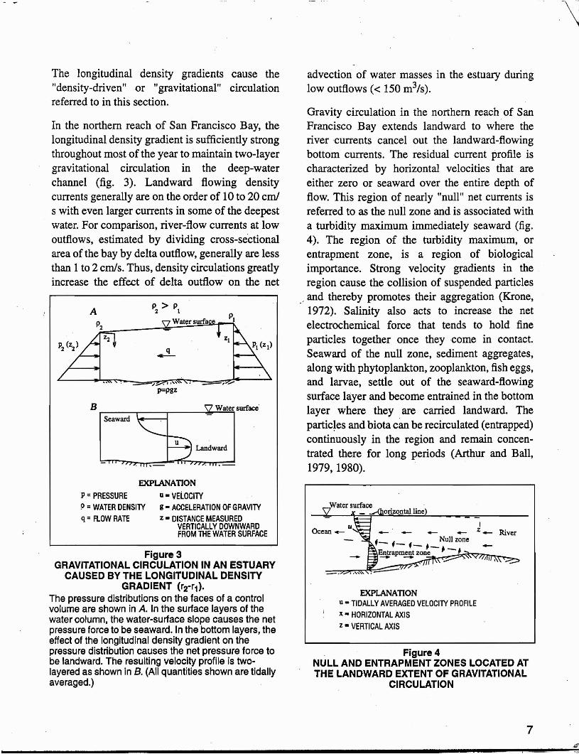
The longitudinal density gradients cause the "density-driven" or "gravitational" circulation referred to in this section.

In the northern reach of San Francisco Bay, the longitudinal density gradient is sufficiently strong throughout most of the year to maintain two-layer gravitational circulation in the deep-water channel (fig. 3). Landward flowing density currents generally are on the order of 10 to 20 cm/ s with even larger currents in some of the deepest water. For comparison, river-flow currents at low outflows, estimated by dividing cross-sectional area of the bay by delta outflow, generally are less than 1 to 2 cm/s. Thus, density circulations greatly increase the effect of delta outflow on the net

"/ ., ," p=pgz

B .--__.--_-r-__~~W.:.::a~tersurface'

Seaward \.----.,,.-1

u Landward

EXPLANATION

P=PRESSURE u- VELOCITY P=WATER DENSITY g - ACCELERATION OF GRAVITY q =FLOW RATE z - DISTANCE MEASURED

VERTICALLY DOWNWARD FROM THE WATER SURFACE

Figure 3 GRAVITATIONAL CIRCULATION IN AN ESTUARY

CAUSED BY THE LONGITUDINAL DENSITY GRADIENT (r2-r1)'

The pressure distributions on the faces of a control volume are shown in A. In the surface layersof the watercolumn. the water-surface slopecausesthe net pressure force to be seaward. In the bottom layers; the effect of the longitudinal densitygradient on the pressure distribution causesthe net pressure force to be landward. The resulting velocityprofile is two­layered as shown in B. (All quantities shown are tidally averaged.)

advection of water masses in the estuary during low outflows « 150 m3/s).

Gravity circulation in the northern reach .of San Francisco Bay extends landward to where the river 'currents cancel out the landward-flowing bottom currents. The residual current profile is characterized by horizontal velocities that are either zero or seaward over the entire depth of flow. This region of nearly "null" net currents is referred to as the null zone and is associated with a turbidity maximum immediately seaward (fig. 4). The region of the turbidity maximum, or entrapment zone, is a region of biological importance. Strong velocity gradients in the region cause the collision of suspended particles

._ and thereby promotes their aggregation (Krone, 1972). Salinity also acts to increase the net electrochemical force that tends to hold fine particles together once they come in contact. Seaward of the null zone, sediment aggregates, along with phytoplankton, zooplankton, fish eggs, and larvae, settle out of the seaward-flowing surface layer and become entrained in the bottom layer where they are carried landward. The particles and biota can be recirculated (entrapped) continuously in the region and remain concen­trated there for long periods (Arthur and Ball, 1979, 1980).

EXPLANATION U - TIDALLY AVERAGED VELOCITY PROFILE x - HORIZONTAL AXIS z - VERTICAL AXIS

Figure 4 NULL AND ENTRAPMENT ZONES LOCATED AT THE LANDWARD EXTENT OF GRAVITATIONAL

CIRCULATION

7

Because tidally-averaged salinity gradients in the northern reach of San Francisco Bay change seasonally and episodically with variations in delta outflow, outflow causes the greatest varia­tion in density currents and location of the null­entrapment zone. As a general rule, the strength; of density currents increases with increasing delta outflow as the null zone moves seaward and the longitudinal salinity gradient is established over a shorter reach of the estuary. The null-entrapment zone generally is found in an area where salinity" is between 1 and 6 (Arthur and Ball, 1979).

In the southern reach of San Francisco Bay, den­sity circulations result in the exchange of waters 'between Central and South Bays. These exchanges usually occur in early winter with the onset of high delta outflows and during late spring with the decline of delta outflows. With the rise or fall of inflow to. North Bay, water densities in Central Bay become less than or greater' than those in South Bay, thereby creating a density gradient that drives the exchanges between the two bays (McCulloch and others, 1970; Walters, 1982).

In addition to delta outflow,the strength of density currents depends on water depth, the intensity of vertical mixing, and tidal energy. Other factors being equal, density currents generally will be larger where the depth of water is greater. In northern San Francisco Bay where channel depths are at aminimum-approximately 11 m below low water at Pinole Shoal in San Pablo Bay and at the western end' of Suisun Bay-the density currents are usually weak' or absent. These shallow channel depths can result in a topographic block on landward flowing bottom currents that originate from deeper waters. The fortnightly spring-neap cycle in the tides also affects the magnitude of density currents. As the amplitude (and energy) of the tide wave varies over a 14-day spring-neap tidal cycle, the amount of vertical mixing and the, strength of gravitational

4Salinity in this report is expressed according to the Practical Salinity Scale, 1978 (Unesco, 1979). The salinity of freshwater is zero and of coastal ocean water near San Francisco Bay is approximately 34.

circulation also will vary. During neap tides when tidal energy and vertical mixing are at a minimum, density currents are greatest. During spring tides, when tidal energy and vertical mixing are at a maximum, density currents are least. The effect the annual cycle in tidal energy has on the magni­tude of density,currents is not well known. During the periods of March and October when monthly averaged tidal energies are the lowest of the year, gravitational circulation for a given delta outflow is probably greater than for other times .during the year with similar outflow, The strong spring tides and weak neap, tides that occur in June and December cause a greater spring-neap variability in density currents" during' those periods than during other times of the year.

" Density-driven circulation plays an important role in biological and water-quality, processes in the bay. It is a 'mechanism '. by which sediment, plankton, invertebrates, larval fish, and contami­nants can move great distances within the system. The landward bottom currents also can bring organisms spawned in the coastal ocean into the estuary and transport them. upstream. Lateral mixing and circulation processes can then transfer the eggs and larvae to nursery grounds in the shoals. (

As noted previously, the position of a null­entrapment zone in the northern reach of San Francisco Bay is determined largely by density circulation and inflow. Providing sufficient flowto position the entrapment zone out of the deeper waters of the Sacramento River and adjacent to the biologically productive shallow areas of Suisun Bay has long been postulated as' being biologically significant, although the data remain unclear on this issue (Kimmerer, 1992). Recently (December 15, 1994) a state-federal agreement was reached calling for an estuarine habitat standard for Suisun Bay, based on a bottom salinity of 2, to be used in managing freshwater discharge to the estuary. The basis for using salinity as a habitat indicator for estuarine biological populations is discussed by Jassbyand others (1995). The location of the entrapment zone is thought to correspond closely with the

8

location of the isohaline associated with a salinity of2.

Horizontal Circulation

The effect of freshwater inflow on net horizontal (vertically uniform) circulation and transport in San Francisco Bay is not well understood. The flow-driven component of horizontal circulation is difficult to identify, except during high flows, because it is dominated bya tidally driven component that is an order of magnitude larger. Wind-driven currents also can be important to horizontal circulation, although the effect in North, Bay is largely unknown because of a lack of current measurements in shallow water where wind effects are greatest,

Because deployment of instruments at more than a few geographic locations' at once is costly, the collection of enough field measurements to analyze fully the patterns of horizontal circulation usually is not. feasible. Multidimensional numerical models, therefore, often are used to study horizontal circulation because they can calculate entire spatial distributions of currents under varying conditions and can isolate the effect on flow from tide and' wind. Models carefully calibrated with field measurements can give reliable results.

During low-flow periods in North Bay, river-flow currents are only 1 to 2 cmls, while the tide­induced residual currents are usually on the order of 10 cmls in Suisun Bay (Walters and ~ others, 1985) and somewhat larger farther seaward. Because of their large magnitude, tide-induced residual currents are an important part of the circulation that produces' longitudinal and transverse mixing in San Francisco Bay.

The tidally driven, residual circulation is the result of tidal currents interacting with the irregular bathymetry in San Francisco Bay and is usually greatest where asymmetries exist between flooding and ebbing currents through a cross­section. Fischer and others (1979) refer to this form of circulation as "tidal pumping." Because of the greater tidal forcing during spring tides, the tidally driven, residual circulation is normally

greater during spring tides than it is during neap tides. This tidally driven flow is in contrast to the density-driven flows, discussed in the previous section, which are weakest during spring tides because of enhanced vertical mixing. Walters and Gartner (1985) discuss how tidally driven and

Idensity-driven flows alternately influence net horizontal circulation in Suisun Bay over 'the spring-neap tidal cycle. During spring tides, a seaward flow across the northern part of Suisun Bay results from the tidally driven, residual flow that dominates the density-driven, landward flow. The south-channel flow is landward during spring tides, which causes the large-scale circulation to be counter clockwise (Walters and others, 1985, fig. 8). During neap tides, the density-driven flow dominates and drives a landward flow into the

,-northern part of Suisun Bay. The large-scale circulation during neap tides, therefore, could be clockwise. The tidally driven, horizontal circulation pattern in San Pablo Bay is unknown, although the geometry indicates a clockwise circulation driven by a tidal jet at the eastern and western boundaries (Walters and others, 1985).

During the wintertime high delta outflows into San Francisco Bay, river-flow induced currents can range from 25 cmls to more than 50 cmls and are easily identified from measured data. These currents generally follow the channel geometry and bathymetric contours of the bay, much like those of a nontidal river. However, because relatively few current measurements are available during high delta outflows, the precise spatial distribution of these currents are not known.

Transport by horizontal circulation, particularly of various materials and organisms back and forth between the deep channels and (biologically productive) shoal areas, is a biologically important phenomena in San Francisco Bay. Some fish species, for example, are transported to shoal areas during the early stages of life, using these areas as a nursery ground before returning to the channels and moving elsewhere within the system or out to sea. Lateral circulation and exchange also can be an important mechanism that produces maxima in turbidity and other

9

properties at the entrapment zone in Suisun Bay. Because wastewater is often discharged into near-shore shallow areas, the flushing times of pollutants from the bay also will depend on the lateral movement of pollutants to deep-water channels where stronger currents can carry them out to sea. The residence time.of water masses in shallow areas are generally affected by lateral exchanges. Walters and others (1985) discuss residence times of water masses in San Francisco Bay and include a table of residence times for the various embayments in the bay.

Salt Transport

Delta outflow has a direct effect on the transport and mixing of salt in San Francisco Bay. During high delta outflows, the salt mass in the northern reach ·of the bay. is displaced from the estuary relatively quickly (from 1 to 3 days), but quickly moves landward as the outflow recedes. Both the net horizontal and the vertical circulation (dis­cussed in the previous two sections) affect the landward salt flux and general mixing of salt. Conomos (1979) estimated that 60 to 70 percent of the upstream salt flux in North Bay is due to net horizontal circulation, such as tidalpumping, and 30 to 40 percent is due to density-driven gravi­tational circulation. Observations in Suisun Bay after a pulse of delta outflow indicate salinity intrudes landward along the channel bottom first and then mixes laterally to the shoals. The salt flux due to gravitational circulation is most dominant during neap tides when stratification is present (Walters and Gartner, 1985).

Although delta outflow isthe dominant cause of variability in mean (tidally averaged) salinity in San Francisco Bay, other factors that can affect variability are dominant during periods of relatively low and steady inflow. Most data records indicate a significant .tfrom 1 to.' 5) spring-neap variability in mean salt concen­trations due to variability in the residual and tidal currents (Walters and others, 1985). The short­term effect ofmeteorological influences or coastal sea-level fluctuations on the variability of salinity within the bay are not well understood, but can be

significant. Cayan and Peterson (1993) discuss the longer term effect of spring climate on interannual variations of salinity in San Francisco Bay. These natural sources of variability in salinity can make controlling salinity in the bay through regulation of upstream flow, such as for a water-quality standard, difficult.

In South Bay, the delta outflow-induced stratifications of salinity that occur during the winter wet season are important because they serve as a control on vertical turbulent mixing. Cloern (1984)· observed that, during periods of prolonged salinity stratification in South Bay, phytoplankton biomass and primary productivity is high in surface layers. Phytoplankton biomass is generally low during dry periods when the

, water column in South Bay is well mixed. Further , research is needed to clarify the effects of unreg­

ulated pulses of winter delta outflow on salinity stratification in South Bay.

The effect of salinity on fish resources probably relates mostly to the physiological salinity tolerance of the fish. However, salinity possibly can have other more subtle effects, such as on the concentration and toxicity ofpollutants and on the overall sensitivity of organisms to pollutants. '.

Because most fish have a range.of salinity in which they do best, salinity influences the move­ment of fish within the estuary. As an example, salinity increases in Suisun Bay are thought. to have caused Delta smelt to shift their habitat use upstream (U.S. Environmental Protection Agency, 1992). Fish are classified in terms oftheir salinity tolerance as marine, estuarine, or fresh­water species.' Marine and freshwater species usually will not be found in areas where salinity changes rapidly. Conversely; estuarine species may thrive in areas of moderate salinities and relatively high rates of change in salinities. Larval fish, generally nonmobile or feeble swimmers, can be affected seriously by rapidly changing salinity levels because of their inability to move to avoid unfavorable conditions. Because long-term reductions in delta outflows will increase salinities in San Francisco Bay, delta outflow changes can affect fish resources.

10

l Chapter 2

FI ELD ACTIVITIES

The two major activities of the hydrodynamic study are field measurements and riumerical modeling. This chapter describes the field activities and is divided into four parts. The first part describes the research vessels and instru­mentation used for field data collection. The second part describes the network of monitoring stations where continuous measurements of water level, 'salinity, temperature, and meteorological data are being collected. The third part presents some analyses of the water-level and salinity data from the continuous monitoring stations. In the fourth part, the actual' field studies that were done are reviewed, with some observations and findings included when they were available.

Research Vessels and Instrumentation

Research Vessels

Early in the study, each agency that participated in the hydrodynamic field program (the USGS, the USBR, and the DWR) acquired research vessels to be used during proposed periods of data col­lection. Each vessel had to be capable of reaching speeds of about 55 km/h. The vessels also needed a reasonably shallow draft for working in shallow waters. Additionally, the USGS vessel needed adequate deck space and' hoisting equipment for deployment and retrieval of current meters.

The USGS and the USBR jointly purchased two new, identical research vessels in 1985. The vessels were 10m long with: aluminum hulls and were powered by dual diesel engines with stem ' outdrives. The vessels were named the RV Saul Rantz (USGS) and the RV Scrutiny (USBR). After delivery of the vessels, each was equipped with radar, _a Loran-C positioning system, a winch, and an anchor. A capstan and an "A" frame were installed on the RV Saul Rantz for hoisting instruments. The RV Saul Rantz was manufactured with an opening in its hull to insert

a transducer array for an acoustic Doppler current profiler.

A 9.1-m-Iong, single engine vessel for use by the DWR was obtained in 1986 by the USBR from a list of Federal surplus property. This vessel had been used as a u.s. Customs patrol boat and needed significant repairs and modifications for use in .the study. The vessel, referred to simply as the "Uniflite," became fully operational in March 1987.

In 1993, after 8 years of using the RV Saul Rantz for the hydrodynamic study, the USGS decided a

"larger vessel was needed for field experiments in which current profilers Were deployed andre­trieved and for servicing monitoring' stations accessible only by boat. A 16.2-m, former fishing vessel was purchased in late 1993 and named the RV Turning Tide. The RV Saul Rantz was sold to the USBR for use in their.biological monitoring programs and was renamed the RV Compliance.

Conductivity, Temperature, Depth Profiling Equipment

Three conductivity-temperature-depth (CTD) profiling systems were purchased in August 1985 for use on each of the three research vessels. The CTD profilers are state-of-the-art systems with sensors that are capable of sampling 24 times per second for measurements of temperature, specific conductance, transparency (similar to turbidity measurement), and sensor depth (pressure). The measurements are recorded as' the instrument rapidly descends through the water column. Salinity is calculated within the system elec­tronics using the measured temperature and specific-conductance data. A shipboard computer stores data from the profiler and graphically displays measurements as they are made. The systems originally were purchased for use in the salinity profiling program, but have since been used in many of the other field studies.

11

Conventional Recording Current Meters

Before the San Francisco Bay hydrodynamic study began, the USGS had 10 recording current meters that were used in earlier studies. These meters measure current speed using a horizontal­axis impeller, a procedure that worked well in deep water deployments made during an intensive USGS and National Oceanic and Atmospheric Administration (NOAA) current measurement study in 1979 and 1980 (Cheng and Gartner, 1984). However, the meters had never been deployed in the shallow waters of San Francisco Bay. To determine if these meters would accu­rately measure currents in the presence of wind waves in shallow water, a current-meter inter­comparison study was carried out in the shallow waters of South Bay during the summer of 1984 prior to the start of the hydrodynamic study. Measurements made using one of the current meters from the existing inventorywere compared with-measurements made using three other meters, each from a different manufacturer. Each of these three meters had a different design for the water­speed sensing system: a vertical-axis rotor, an inclinometer, and an electrom.agnetic probe. The instruments were deployed side-by-side at a height of 1.2 m above the bottom of the bay in water that varied in depth between 2 and 5 m during the study period. A comparison of velocity records indicated that measurements by the vertical-axis rotor and inclinometer meters were significantly affected by wind waves; the horizontal-axis impeller and electromagnetic probe meters, however, did well. On the 'basis of these results, the existing inventory of horizontal­axis impeller meters was considered appropriate for use in future shallow, as well as deep-water, deployments. Detailed results from the inter­comparison study are available in reports by Gartner and Oltmann (1985; 1990).

Downward-Looking Acoustic Doppler Current Profiler

Acoustic Doppler current profilers (ADCPs) are state-of-the-art instruments used to .measure

velocity profiles in oceans and, more recently, in estuaries and rivers. In 1985, the USGS purchased the first commercially available, shallow-water ADCP for use in the hydrodynamic study of San Francisco Bay. The instrument is referred to as "downward-looking" because it is operated using a transducer array that points vertically downward from the water surface and normally is mounted on a platform or in a research vessel. In this case, the transducer array was first mounted in the hull of the USGS research vessel, the RV Saul Rantz.

The ADCP originally was purchased for use in the salinity profiling program so that velocity profiles could be collected, along with salinity profiles, in the deep water channels of San Francisco Bay at ' varying outflows. The instrument also was used to collect velocity data for validating a 3-D model

.:and to measure tidal flows within the estuary by integrating velocity profiles as the research vessel traversed across the estuary. An ADCP. flow measuring system was developed and is described later in this section. The ADCP is a relatively new technology (particularly for use in shallow-water estuaries); therefore, a brief review of the prin­ciples of operation and the field tests used to test the instrument accuracy follows.

Principles of acoustic Doppler current profiler operation

An ADCP operates using an 'array of four trans­ducers that continuously transmit short acoustic pulses, or "pings," into the water column beneath the instrument at angles inclined 30 degrees from vertical. Part of the transmitted sound from each . ping is reflected backward, or is "backscattered," to the transducers from' sound scatterers in the water. The sound scatterers are small suspended particles or plankton that occur everywhere in a water body and move at' the same velocity as the water. In accordance with the Doppler principle, the frequency of the backscattered sound is shifted by an amount that is proportional to the relative velocity between the scatterers and the transducer assembly. The·water velocities are computed first as components along each beam

12

axis and later are converted to three orthogonal components in the north, east, and vertical directions by the shipboard computer. Normally, only the two horizontal components are saved. Because the ADCP samples backscattered sound from each beam at O.l-second intervals, water .velocities can be resolved at depth intervals of 1 m; these intervals are called bins. Measurements are made over approximately 75 percent of the water column. Because of acoustic-beam inter­ference with the boundaries, the near-surface and near-bottom layers are excluded. The velocity measured for each bin is considered to be the aver­age water velocity through the 1-m horizontal slice of the water column bounded by the four acoustic beams.

.. Using a separate acoustic pulse, the velocity of the channel bottom relative to the ADCP, which is equivalent to the vessel velocity, also is deter­mined. This procedure is referred to as bottom tracking. The vessel velocity is used to compute water velocities relative to an Earth-based reference frame.

Although originally developed to measure 3-D current velocities, ADCPs also are used for meas­uring the concentration of suspended material (sediment) in water bodies (Thevenot and Kraus, 1993). The concentration is estimated from ADCP backscatter intensity, which can be calibra­ted with independent measurements of suspended material. By simultaneously measuring water velocity and suspended material concentration, the ADCP holds promise for directly measuring particulate flux. For a further description of ADCP operation, refer to RD Instruments (1989).

Field tests for accuracy of the acoustic Doppler current profiler

Shortly after the delivery of the ADCP, field tests were done to evaluate the accuracy of the instru­ment. The first test was on a lake where the instru­ment was operated from a vessel that was navigated over a straight-line course of precisely measured distance. The ADCP system was used to estimate the distance traveled by the vessel

using bottom-tracking data. The average error in the distances calculated by the ADCP during 13 test runs, using various boat speeds and two directions of travel, was 1.9 percent. Water

.velocities measured by the ADCP were used to estimate quantitatively a short-term random error of-the instrument. Because water in the lake was motionless, any water velocities detected by the ADCP were attributed to random error of the instrument. This random error was evaluated for various averaging periods of the profiler data. The error using a l-second averaging period was 6.5 cm/s; but, for a 20-second averaging period, the error was reduced to 2.3 cm/s. Further averaging reduced the error still more. Simpson (1986) presents the results of the testing in the form of a curve that relates the measurement error

,_ to the averaging period.

A second test of. the instrument was done on a river under moving water conditions. Velocities were measured by the ADCP from an anchored vessel and then were compared with those meas­ured using Price AA and electromagnetic current" meters. The results indicated that the' ADCP measurement errors for moving water were essentially equal to those for still water (Simpson, 1986). The accuracy specifications determined by the tests agreed well with those supplied by the manufacturer. The ADCP provides accurate measurements of currents as long as an averaging period of 20 seconds or more is used.

Acoustic Doppler current profiler discharge measuring system

Development of an ADCP discharge measuring system began in October 1987. The USGS hydro­dynamics study team wrote a computer program that uses the velocity profiles and bottom-tracking data from the ADCP, along with water-depth data provided by a sonic sounder, to integrate flow as the profiler is transported across a channel. Procedures are incorporated into the program to compute total cross-sectional flow by estimating flow in the unmeasured parts of the cross section near the shoreline and in the surface and bottom

13

p

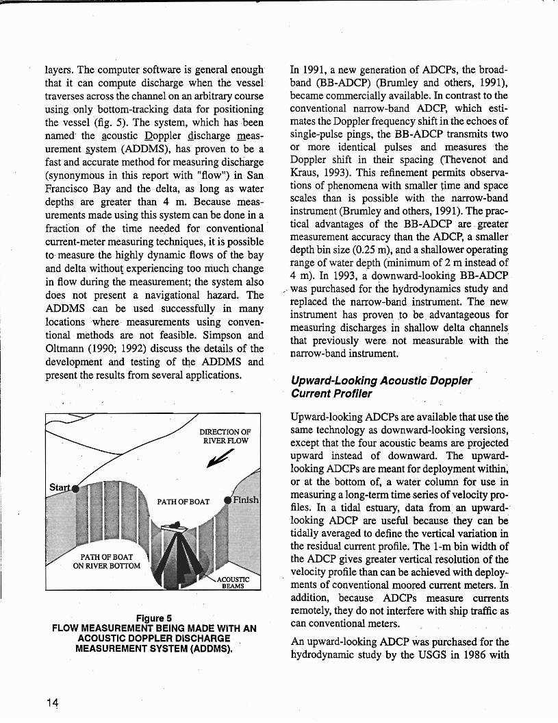
layers. The computer software is general enough' that it can compute discharge when the vessel ' traverses across the channel on an arbitrary course using only bottom-tracking data for positioning the vessel (fig. 5). The system, which has been named' the gcoustic Doppler 4ischarge meas­urement ~stem (ADDMS), has proven to be a fast and accurate method for measuring discharge (synonymous in this report with "flow") in San Francisco Bay and the delta, as long as water depths are greater than 4 m. Because meas­urements made using this system can be done in a fraction of the time needed for conventional ' current-meter measuring techniques, it is possible to measure the highly dynamic flows of the bay and delta without experiencing too much change in flow during the measurement; the system also does not present a navigational hazard. The ADDMS can be used successfully in many locations where measurements using conven­tional .methods are not feasible. Simpson and Oltmann (1990; 1992) discuss the details of the development and testing of the ADDMS and present the results from several applications.

DIRECTION OF RIVER FLOW

PATHOF BOAT

PATHOF BOAT ONRlVER BOTTOM

Figure 5 FLOW MEASUREMENT BEING MADE WITH AN

ACOUSTIC DOPPLER DISCHARGE MEASUREMENT SYSTEM (ADDMS). .

In 1991, a new generation of ADCPs, the broad­band (BB-ADCP) (Brumley and others, 1991), became commercially available. In contrast to the conventional narrow-band ADCP, which esti­mates the Doppler frequency shift in the echoes of single-pulse pings, the BB-ADCP transmits two or more identical pulses and measures the Doppler shift in their spacing (Thevenot and Kraus, 1993). This refinement permits observa­tions of phenomena .with smaller time and space scales than is possible with the narrow-band instrument (Brumley and others, 1991). The prac­tical advantages of the BB-ADCP are .greater measurement accuracy than the ADCP, a smaller ' depth bin size (0.25 m), and a shallower operating range of water depth (minimum of 2 m instead of 4 m). In 1993, a: downward-looking BB-ADCP

-:was purchased for the hydrodynamics study and replaced the narrow-band instrument. The new instrument has proven tobeadvantageous for measuring discharges in shallow delta channels that previously were not measurable with the' narrow-band instrument.

Upward-Looking Acoustic'Doppler Current Profiler

Upward-looking ADCPs are available that use the same technology as downward-looking versions, except that the four acoustic beams are projected upward instead of downward. The upward­looking ADCPs are meant for deployment within; or at the bottom of, a water column for use in measuring a long-term time series of velocity pro­files. In a tidal estuary, data from , an upward­looking ADCP are useful because they can be tidally averaged to define the vertical variation in the residual current profile. The l-m bin width of the ADCP gives greater vertical resolution of the velocity profile than can be achieved with deploy­ments of conventional moored current meters. In , addition, because , ADCPs measure currents remotely, they do not interfere with ship traffic as can conventional meters.

An upward-lookingADCP was purchased for the hydrodynamic study by the USGS in 1986 with

14

funds provided by the USACOE. To deploy the instrument, a specially designed platform was made of corrosion-resistant copper-nickel alloy. This platform rests on the bay bottom and posi­tions the ADCP transducer head at a point about 0.7 m above the bed. The vertical measurement region of the ADCP begins at about 2.1 m above

, the bed and extends to about 2.5 m below the surface. The loss of profiling region near the sur­face is characteristic of the ADCPs and is the result of acoustic beam interference with the water surface.

Data from an ADCP can be transmitted to shore by an underwater cable or can be stored on a memory device in the instrument casing. The ADCP purchased for the hydrodynamic study was initially configured for operation using a cable, but was later (1989) converted to a self-contained unit so that it could be deployed without requiring an instrument shelter on shore. Data from an ADCP are processed and stored using a time cycle that is user-specified. For all deployments in San Francisco Bay, a data-collection time cycle of 10 minutes was used. During each 10-minute cycle, the ADCP determines more than 1,500 in­stantaneous velocity profiles, vector averages the results for each l-m depth bin, and records the final velocity profile.

The ADCP must be deployed and retrieved using a vessel equipped with adequate hoisting equip­ment for lowering and raising the instrument and platform. Each deployment requires a dive team who level the instrument to within its allowable limits. A float and hoisting .line are released acoustically from the platform to the surface for retrieval.

In 1992, the USGS purchased a second upward­looking ADCP for use in the hydrodynamics study. The instrument was used in early 1993 during a field experiment in Suisun Bay, which is discussed later in this report. Both upward­looking ADCPs are narrow-band instruments. The broad-band technology mentioned in the previous section also is available in upward­looking instruments. Ralph Cheng (USGS, Menlo Park) acquired three of the broad-band

instruments and loaned these instruments to the study team for use in field experiments in 1993, 1994, and 1995{see Chapter 5).

Continuous· Monitoring Stations

- In San Francisco Bay, there are significant spatial . variations' and annual, seasonal, diurnal, and

semidiurnal oscillations in water height, and sa­linity as well, that are related to tides, fresh-water inflow, and meteorological forcing. To a lesser degree, there are variations in temperature. By continuously monitoring water-level, salinity, and temperature at various locations in the bay, long­term time-series data are obtainedthat can be analyzed to separate and quantify the degree of variability in these parameters as a result of dif­

>ferent forcing mechanisms. The effect of fresh­waterinflow on salinity, for example, is of partic­ular interest. Time-series data.are.also important for numerical model studies because they are. needed to define boundary conditions and to calibrate and verify the models. .

. As part of the hydrodynamic study, the USGS and the DWR presently (1995) maintain a network of eight monitoring stations where water. tempera­ture and specific conductance are recorded contin­uously at 15-minute intervals. At four of these stations, water level also is recorded. Salinity is computed directly from the specific-conductance data. The locations of the stations, the types of data collected at each station, and the period of. record are identified on figure 6 with the specific­conductance monitoring stations shown as salin­ity stations. Because the degree of vertical. strati­

; fication in salinity and temperature is of interest, six of the stations-e-San Mateo Bridge, Bay Bridge, Point San Pablo, Selby, Martinez, and Mallard Island-record water temperature and specific conductance at two depths, one near the surface and another at approximately mid-cross­section depth. The longest periods of record began in the early 1980's. However, the data records are not continuous from that time because of numerous periods of instrument failure and other problems that resulted in missing or bad data.

15

122°30' 122°00'

EXPLANATION DATA COLLECTED DATA AVAILABLE FROM

• WATER LEVEL, SALINITY,AND TEMPERATURE

• SALINITY AND TEMPERATURE

• METEOROLOGICAL

A STATION OPERATED FROM AUGUST 1988-APRIL 1990

B STATION OPERATED FROM JULY 1991-PRESENT (1994)

C STATION OPERATED FROM AUGUST 1988-JANUARY 1994

STATION WATER' SALINITY NAME LEVEL AND TEMP.

MAL SEPT. 86 JUNE 84 MTZ JUNE86 MAR. 83 WIC OCT. 86 OCT. 86 PSP JUNE86 OCT. 83 FPT -­ OCT. 90 BBR - JAN. 83 5MB -­ NOV. 81 DUM SEPT.a9 SEPT. 89

o 5 10 ,I1---,...-----'-...,...1--......1 MILESI

o "5 10 KILOMETERS

Figure 6 LOCATIONS OF CONTINUOUS MONITORING STATIONS IN SAN FRANCISCO BAY, CALIFORNIA, AND

TYPESOF DATACOLLECTED BY THE U.S.GEOLOGICALSURVEYAND THE CALIFORNIA DEPARTMENT OF WATER RESOURCES. _

Salinityat the sites shown is computed from a measurement of specificconductance.

16

In addition to the salinity and water-level stations, the USGS has operated two meteorological sta­tions in San Francisco Bay since August 1988. The stations are mounted on channel markers in San Pablo and Suisun Bays (fig. 6). The Suisun Bay station was originally at the site marked A on figure 6 until April 1990. At that time, the station was destroyed, presumably by a passing vessel. A replacement station was installed in July 1991 at the site marked B on figure 6. Wind speed and direction and air temperature 'at 15-minute intervals are recorded at each station. The Suisun Bay station also collected atmospheric pressure data from July 1989 until the station was de­stroyed in April 1,990. Atmospheric pressure data

,have been collected at the San Pablo Bay station (site C, fig. 6) since October 1990. Data collection at the San Pablo Bay station was suspended on January 12, 1994 because the need for additional data at the site is not urgent, The instrument shelter was not removed from the station, how­ever, so that data collection can be resumed when necessary.

The data stations operated by the USGS and the DWR are not the only continuous recording stations for water level, salinity, or temperature available in San 'Francisco Bay. The NOAA operates stations at Alameda, Port Chicago, and Fort Point where continuous, 6-minute interval, water-level data are collected. The Fort Point station has been operational for more' than 100 years. NOAA also recently (1995) installed 3 salinity monitoring stations in Suisun Bay. The USBR also collects continuous electrical conduc­tivity and temperature data at two stations in Suisun Bay, although only daily maximum, mini­mum, and mean values are saved at these stations. One additional source of water-level, salinity..and temperature time-series data is available from a joint NOAA and USGS field study conducted in 1979 and 1980. During that study, numerous deployments of current meters were made for periods of 1 month or longer with electrical con­ductivity and temperature recorded on each meter. Water-level observations were made during this same period at 10 stations along the shoreline, of the bay. These data are described in a series of

USGS reports (Cheng and Gartner, Parts I-V, 1984). Almost all data from the continuous moni- . toring stations described above are included in a hydrodynamic data base that is discussed later in the report.

Analysis of Water-Level and Salinity Monitoring Station Data

The monitoring station data are presently (1995) being analyzed using digital low-pass filters and the technique of principal components analysis to understand how subtidal variations in water level and salinity are related to forcing from the tides, freshwater flow, and meteorological factors in San Francisco Bay. A few selected examples from the analyses that were completed using digital filters

" are presented in the next two sections to illustrate the work that is being done. In the first section, the significant fortnightly (spring-neap) and annual cycles in tidal energy that exist within San Francisco Bay are illustrated. In the second section, the variations in stratification in, the bay caused by the spring-neap cycle and delta outflow are discussed.

The digital filtering is done using a Godin tidal filter(Godin, 1972) that consists of applying three consecutive sequences of moving averages to a time series: the first two sequences using 24-point averages (assuming hourly spaced data) and the third using 25-point averages. The filter effec­tively removes the tidal and shorter-period varia­tions from the time series and passes the slowly varying subtidal variations. An illustration of the Godin filter applied to a salinity time. series at Point San Pablo is shown on figure 7 where the filtered curve represents the variation in tidally averaged salinity. In the example, the filtered time series shows the effect of runoff that began about day 46.

Spring-Neap and Annual Cycles in Tidal Energy

Energy input for mixing in San Francisco Bay is derived primarily' from the tides, wind, and freshwater inflow. Under most circumstances, tides are the dominant source of mixing in the bay.

17

~ ~ ..J C1j

--- NEAR SURFACE -lOW-PASS FilTERED

45 50 55 60 65 70 75 80

5

10

25

20

15

DAYS FROM JANUARY 1,1986

Figure 7 . NEAR-SURFACE AND LOW-PASS FILTERED

SALINITIES AT POINT SAN PABLO, SAN FRANCISCO BAY, CALIFORNIA.

A measure of tidal energy is RMS (root-mean­square) tide height defined by

RMSk = «hk-h"J2>1I2 where

hk is a measured time series of water level at times tk = k X L\t,

h is the mean water level, and m

< > denotes that a Godin filter is used to compute a tidal mean of tide height squared.

Computed in this manner, tides are. the major component of variation in RMSk, although other factors that affect water level (atmospheric pressure, wind set-up, and delta outflow) also are included.

The variations in RMS tide heights for calendar year 1989 are shown on figure 8 for the four water-level monitoring stations in North Bay identified on figure 6 and the NOAA water-level monitoring station at Fort Point. On each graph, the horizontal line is the annual mean RMS value computed by simple averaging of the RMS time series. The most apparent variations in RMS about the mean are the fortnightly oscillations due to the spring-neap tidal cycle. This strong spring-

neap variability in tides causes a corresponding spring-neap variability in tidal currents in San Francisco Bay that plays an important role in mixing. The effect of the spring-neap cycle on density-driven gravitational circulation was dis­cussed in Chapter 1. The spring-neap variability is greatest near the Golden Gate at Fort Point before the incoming tides are modified by bay geometry and the increased friction from shallow water. Progressing landward from the Golden Gate, spring-tide amplitudes uniformly decrease, whereas neap-tide amplitudes increase slightly up to Selby at the western end of Carquinez Strait, then decrease through the strait and Suisun Bay. The annual mean RMS value remains relatively constant between 0.55 and 0.57 m up to Carquinez Strait and then drops off markedly through the

.> strait and Suisun Bay.

As the tide wave propagates into San Francisco Bay, there are competing tendencies for the wave height to both amplify and dissipate. The wave height tends to amplify as its energy funnels into shallower water and becomes confined. Wave re­flection off shorelines also serves to amplify the wave height. The wave height tends to dissipate because of the increased frictional effects in shallow water and energy losses at constrictions such as San Pablo and Carquinez Straits. Friction and constriction losses have the greatest effect when tidal currents are strong, which most likely explains the observed decrease in tidal amplitudes proceeding landward on spring tides. During neap tides when tidal currents are weak, friction and constriction losses are less important, and the slight amplification of the tide wave as it pro­gresses up through San Pablo Bay probably is due to the greater importance of geometric effects.

Evidence of an annual tidal cycle is present at all five stations, but is most significant at the seaward stations (fig. 8). Large amplitude spring tides and small amplitude neap tides occur during -the months of June and July (days 152-212) and December and January (days 335-365 and 0-31). Small amplitude spring tides and large amplitude neap tides occur during March (days 60-90) and in late September and early October (days 260-280). The exact timing of spring and neap tidal maxima

18

400

A

35030025020015010050

0.8 r-----.,-----.......~--__r-~-__,.----r__---_r_---__r_---....,

0.7

0.6

0.5

0.4

0.3 a

0.8 B

en 0.7 a: w 0.6 WIC.... w ~

0.5 ~ ...... 0.4::J: C!J , tn 0.3::J: w a 50 100 150 200 250 300 350 400 c j::: wa: -e =>

0.8c en CI z 0.7tiS PSP ~ 0.6~ 0 0 0.5a:

0.4

0.3 0 50 100 150 200 250 300 350 400

o FPT

350 400300 .150 200 250

DAYS FROM JANUARY 1.1989

10050

0.8 ....._----r-----__r_---~---~----....._---__---~---_,

0.7

0.6 I+-++-+-+--++-+--+-~_I_--+-~_+_t_+_++_+_+_++_+_+_++_+___f__+_ll_+__+_+_;..........,J_lr____I'r__+_+_+_++_+_+_

0.5

0.4 0.3 L....- ­ ....L­ ......L... ----L.. -I. L.... ­ ...l.....­ ......L...­ ......

o

Figure 8

ROOT-MEAN-SQUARE TIDE HEIGHTS FOR 1989 COMPUTED FROM WATER-LEVEL DATA COLLECTED AT (A) MALLARD ISLAND (SOLIDLINE)AND MARTINEZ (DASHED LINE),(B) SELBY(WICKLANDOIL PIER), (C)

POINTSAN PABLO, AND (D) FORTPOINT(GOLDEN GATE), SAN FRANCISCO BAY, -CALIFORNIA.

The horizontal lineon each graphis the annual mean RMSvalue.

19

and minima varies.slightly from year to year, but the annual cycle repeats itself each year. The data collected during 1985-89 near the Golden Gate at Fort Point (fig. 9) indicate that winter and summer are periods of high variability (strong spring tides .and weak neap tides) and spring and fall are periods of low variability (weak spring tides and strong neap tides). Theone exception is spring 1986 when the weakest neap tide of the year occurred during a period of very high flows in March. The dashed line on figure 9 is a 30-day moving average of the RMS tide height, which illustrates that spring and fall are also seasons of lower than average overall tidal energy when

.'averaging over the spring-neap cycle is considered.

Variations in Salinity Stratification

During most years, several large delta outflows to San Francisco Bay occur. These outflows create 'conditions of greatly reduced salinity and in­creased stratification in the northern reach of the bay that persist until the outflow recedes and mixing returns the estuary to antecedent conditions. The degree of stratification is influ­enced by the water buoyancy from delta outflows and by the amount of vertical mixing derived from the energy in the tides. Cloern (1984), Walters and others (1985), and Smith and others (1991) have discussed the effect of the spring-neap cycle in­tidal energy on vertical stratification. Stratifica­tion is greater during neap tides than during spring tides because of the smaller vertical mixing, The effect of the annual cycle in the tides on strati­fication is difficult to identify clearly, but it is. likely that, during the spring and fall seasons when the long-term tidal energy reaches an annual minimum (fig. 9), salinity stratification will be maintained for-longer periods.

An example of the response of mean salinities at the Selby station (WIC) (fig. 6) to moderate runoff during March 1989 is shown on figure 10. Salin­ities measured at both surface and mid-depth decreased by over 15 during the month of March (days 60-91) and did not recover to previous levels until July (days 182-200). The low-pass filtered salinity stratification during the period

(fig. lOb) rose to more than L\S=l m-I and re­mained above LlS=0.2 lll-l until after the end of April (day 120). These data indicate that the effects of inflow on salinity can be large and can occur over an extended period of time.

Any effect of the spring-neap tidal cycle on strat­ification following the period of runoff is not . evident in figure lOb because of the missing data. Although the stratifications generally are low, the oscillations between approximately LlS=O.O m-I

and 0.3 m-I prior to the period of runoff seem to be related to the spring-neap cycle. -The effect of the spring-neap cycle on stratification is even more evident during the period of runoff in Feb­ruary 1986 when the largest peak runoff was recorded for the San Francisco Bay stations; the peak was also among the largest estimated during

" the past 150 years. The peak occurred on February3/s20 (fig. l ld, day 51) and was 17,800 m

(630,000 ft3/s). Salinities in the bay decreased rapidly during that week (fig. lla-c), reaching a minimum on February 21 (day 52) at.Point San Pablo and on February 23 (day 54) and February 24 (day 55) at the Bay Bridge and San Mateo Bridge, respectively. The stratifications measured during runoff at the three monitoring stations are

, shown on figure 12(a-c). Minima of tidal energy occurred during neap tides on days 47, 61, 77, 92, and 106 (shown as vertical lines on fig. 12a-d). These minima actually precede the maximum values of mean stratification by afew days.

Studies

Hydrodynamic field studies of San Francisco Bay began in 1985. A brief description of each study, along with the results and findings that are

.available, are given below. When appropriate, references are given for reports that include additional information or data summaries.

Salinity Profiling Program

The first field study was a program to measure the . verticaldistribution of salinity, temperature, and

transparency in the channels of North Bay at various outflows. Twenty-two profiling runs were made in which one, two, or three research vessels

20

0.8 r------r------r------r-----r-----r-----,..-------flrr---------,

0.7

0.6

0.5

0.4 0.3 __----'L.........._....:.....-_L- L--:--__L..._ L....- L..- .L-- ...L....-

o 50 100 150 200 250 300 350 400

DAYS FROM JANUARY 1,1985

~ L- L-_~-L----.L...----L...----L..----.L-----...L....-------'

:I: 0 50 100 150 200 250 300 350 400 w o DAYS FROM JANUARY 1,1986i= wc:::3 0.8 .---r.---r-----.-----.--------,,----,----y-----.-------, o ~ 0.7 L5 ::2: 0.6 § 0.5oc::

0.4 0.3 L-__----I. --'- ...J.... ..J..... .L.....-__----I ----L.. ---'

o 50 100 150 200 250 300 350 400

DAYS FROM JANUARY 1,1988

0.8 r--JI----r------r------,rr---pt---~---y-----.--____:rr_r-_r_-----,

0.7 en ffi 0.6 I:i::i ::2: 0.5 ~ 0.4 . ~ 0.3

0.8 ,....------,------,--------.----.------.-------,r---:--"'""jIT------,

0.7

. 0.6

0.5

0.4 0.3 L­ __----L .....l ­ ..L-__----L ----l... ......L.­ ..L... ­__---I

a 50 100 150 200 250 300 350 . 400

DAYS FROM JANUARY 1,1989

Figure 9

ROOT-MEAN-SQUARE TIDE HEIGHTS FOR1985, 1986, 1988, AND 1989 COMPUTED FROMWATER-LEVEL DATACOLLECTED NEAR THE GOLDENGATEAT FORT POINT, SAN FRANCISCO BAY, CALIFORNIA.

the dashed lines are 30-day movingaverages of the root-mean-square tide heights.

21

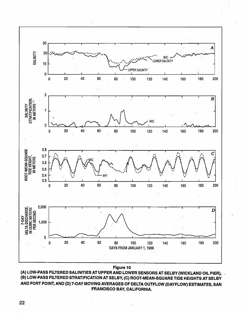
30

~ 20 Z :::i <C en 10

0

2 2-.... O·

~-en~a:-Uw

~u::tu...J_ <C~~ena:Z...-­en

'0

w 0.8a: <C

0.7S'-:chen::I:a:.C!Swz-...- 0.6 Li5~w :!:w~ .CZ 0.5 bi=­ 0.40 a: 0.3

A

0 20 40 60 80 100 120 140 160 180 200

B

0 20 40 60 80 100 120 140 160 180 200

C

0 20 40 60 80 100 120 140 160 180 200

D

20 40 60 80 100 120 DAYS FROM JANUARY 1.1989

140 160 180 200

Figure 10 <

(A) LOW-PASS FILTERED SALINITIES ATUPPERAND LOWER SENSORS ATSELBY(WICKLAND OIL PIER), ( (B) LOW-PASS FILTERED STRATIFICATION ATSELBY, (e) ROOT-MEAN-SQUARE TIDEHEIGHTS ATSELBY ANDFORTPOINT, AND(D) 7-DAYMOVING AVERAGES OF DELTA OUTFLOW (DAYFLOW) ESTIMATES, SAN

FRANCISCO BAY, CALIFORNIA.

---

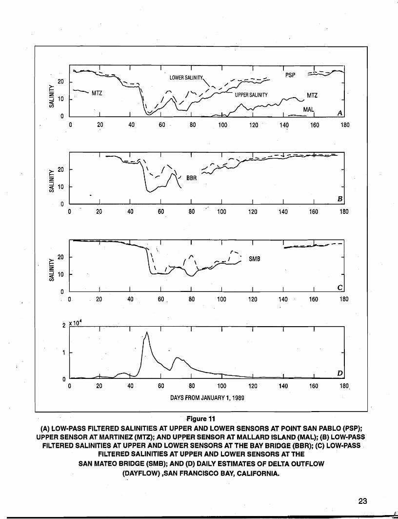
20 ~ Z :J 10 ~

o o 20 40 60 80 100 120 . 140 160 180

~ 20 Z ~ 10 Cf.l

B o o 180

~ 20 Z ~ 10 Cf.l

co . 0 20 40 60 80 100 120 140 160 180

D

20· 40 60 80 100 120 140 160 180

DAYS FROM JANUARY 1,1989

-Figure 11 (A) LOW-PASS FILTERED SALINITIES AT UPPER AND LOWER SENSORS AT POINT SAN PABLO (PSP);

UPPER SENSOR AT MARTINEZ (MTZ); AND UprER SENSOR AT MALLARD ISLAND (MAL); (B) LOW-PASS FILTERED SAlINITIE;S AT UPPER AND LOWER SENSORS AT THE BAY BRIDGE (BBR); (e) LOW-PASS.

FILTERED SALINITIES AT UPPER AND LOWER SENSORS AT THE .

SAN MATEO BRIDGE (SMB); AND (D) DAILY ESTIMATES OF DELTA OUTFLOW

(DAYFLOW) ,SAN FRANCISCO BAY, CALIFORNIA.

23

w 1.00: « =>'-:(1)0::C0: 0.8 C?C'wZi::LH­i:iS::c w 0.6::iEw~ t-!-9~ 0 .... 0.4 0 0:

0.2 0 20 40 60 80 100 120

DAYS FROM JANUARY 1,1989

140. 160 180

Figure 12

LOW-PASS FILTERED SALINITY STRATIFICATION AT (A) POINT SAN PABLO (PSP),

(B) BAY BRIDGE (BBR), AND (C) SAN MATEO BRIDGE (SMB); AND (D) ROOT-MEAN-SQUARE

TIDE HEIGHTS COMPUTED FR~M WATER-LEVEL DATA COLLECTED AT FORT POINT (FPT) AND SAN MATEO"BRIDGE (SMB), SAN FRANCISCO BAY, CALIFORNIA. .

Thedashed vertical lines indicate neap tides that occurred on days 47,61, 77,92, and 106.

24

l

traveled from the Golden Gate Bridge up" the northern estuary, stopping at 2-km intervals to collect profiles using the CTD profiler.

On each profiling run, one vessel traveled up the centerline of the deep-water channel and each additional vessel traveled up one side of the channel. On all runs, the collection of profiles continued landward until salinities were less than 0.5 (landward of the freshwaterlsaltwater inter­face). In places where the channel bifurcates, such as Suisun Bay and the delta, the established route for runs involving a single vessel was to follow the southernmost channel in Suisun Bay and the Sacramento River in the delta; on runs involving two or three vessels, each additional vessel followed one of the two northern channels in Suisun Bay around Roe andlor Ryer Islands and one vessel would follow the San Joaquin River in the delta. On all multivessel runs, the centerline vessel was the USGS vessel RV Saul Rantz, which, in addition to CTD profiles, collected velocity profiles measured with the downward­looking ADCP. A key feature of the study design was that each vessel attempted to collect data while keeping up with the tide wave propagating up the estuary so that tidal phase was a constant for each data set collected. This sampling strategy became known as "running-with-the-tide."

The program, as originally planned in 1985, was to be a joint exercise among the USGS, the USBR, and the DWR using all three research vessels on every profiling run and doing a large number of runs. A dozen or so different delta outflows were to be sampled for tidal phases of high slack, 'low slack, flood, and ebb. Spring and neap tides also were to be sampled for low delta outflows'of less than 425, m3/s (15,000 ft3/s). When the program got fully underway in 1986, other commitments by agency personnel made it unfeasible to sched­ule runs as frequently as originally planned. Because the DWR was unable to provide a research vessel for the first 2 years of the study, their participation was limited to two specially scheduled profiling runs in fall 1988. These two runs were the only three-vessel runs made.' All other runs were made in 1985 or 1986 and were carried out with one or two research vessels

staffed by the USGS and the USBR. Because lowering the CTD profiler turned out to be least difficult during slack water, most runs were made during a slack tide.

The first profiling run was made on October 11, 1985. Because it was intended as a trial run, it started near the San Rafael Bridge (instead of the Golden Gate Bridge) and involved only one ves­sel (the USBR vessel RV Scrutiny). A second test run was made on November 7, 1985, and involved both the USBR and the USGS vessels and started at the Golden Gate Bridge. The run continued landward to Rio Vista on the Sacramento River and required about 2-1/2 hours to complete. Both trial runs confirmed that, during relatively calm wind conditions, it was possible to stop 'and collect profiles at 2-km intervals and still progress

.:up the estuary at a fast enough rate to keep up with the tide wave. The vessels did fall slightly behind the tide wave on both runs, but the amount was insignificant and, in later runs, generally was compensated for by leaving slightly ahead of schedule from the Golden Gate Bridge. Following the successful trial runs, the agencies participating in the hydrodynamic field study decided to pro­ceed with the planned profiling program in 1986. Two intensive periods of profiling runs were carried out in the spring and fall of 1986 during a high- and low-flow period, respectively.

Before the' planned series of spring runs, two unscheduled runs were made in February 1986 during the record high delta outflows that oc­curred that month. On February 20, flow peaked at 17,800 m3/s (630,000 ft3/s). Four days later on

3/sFebruary 24, with a delta outflow of 8,900 m(313,000 ft3/s), the USBR made a profiling run from the Golden Gate Bridge to that part of San Pablo Bay where freshwater was reached. On the following day (February 25), a second run was made using two vessels and again ended in San Pablo Bay. The data indicated intensely stratified conditions in the estuary. At the Golden Gate Bridge, salinities of 12 to 15 were measured in the upper 4 to 5 m and increased to 31 to 33 hear the bottom. In San Pablo Bay, the upper 80 percent of the water' column was essentially freshwater with salinities near the bottom ranging between

25

12 and 24 depending on location. The vertical density gradient in San Pablo Bay occurred over 1 or 2 m of the water column, and velocity shear across the gradient was extremely high; about 1 to 2 mls. On February 24, the USBR also made an unscheduled run through South San Francisco Bay to record conditions there during the high outflow. Conditions in the northern end of South Bay (near the Bay Bridge) were intensely strati­fied with surface' salinities near 5 and bottom salinities near 25. At the extreme southern end of South Bay, the water column was well mixed and had a salinity of about 12.

The planned spring profiling period began in mid­March 1986 and continued for about 1 month. Ten profiling runs were made on the March and April dates listed in table 1. From March 13 to May 2, 1986, seven recording current meters. were de­ployed in mostly shallow-areas of Suisun and San Pablo Bays. The data were collected to estimate water exchanges between the channels and shoals during the salinity sampling. During this period, the estuary was in transition from a high to a medium delta outflow. The unsteady conditions made it possible for a wide range of delta outflows to be sampled in a relatively short period of time.

A planned fall profiling period began in early October 1986 and continued for about 3 weeks, Seven profiling runs were made between October 9 and October 24 (table 1). Five current meters were deployed'during the period from September 23 to November 4, 1986, and seven meters (at three locations) were deployed by OceanSurveys Inc. (under an agreement with the San Francisco State University Tiburon Center for Environ­mental Studies), during the period September 28 to October 29, 1986. The profiling runs during October 1986 were made during low delta out­flows, but included both' spring 'and neap tidal conditions.

, Two three-vessel profiling runs were made on October ,19 and, 25, 1988, to. measure salinity conditions under extreme low delta outflows of 109 m3/s (3,860 ft3/s) and 118 m3/s (4150 ft3/s),

respectively, The October ,19 run was at high slack water o,n a neap tide, and the October 25 run was

Table 1 , .

SAN FRANCISCO BAY, CALIFORNIA, SALINITY PROFILING RUNS

[Vessels per run, number of vessels used during the run; Delta outflow, in cubic meters per second]

Date Vessels per run Delta outflow

October 11, 1985 1 51 November 7, 1985 2 48 February 24, 1986 1 8,870 February 25, 1986 2 7,850 March 20, 1986 . 1 4,700 March 25,1986 2 3,180 March 27, 1986 1 '2,840 March 28, 1986 2- 2,730 April 1, 1986 1 2,270 April 2, 1986 2 2,210 April 4, 1986 1 1,950 April 8, 1986 2 1,870 April 10, 1986 1 1,800 April 18, 1986 1 1,180 October 3, 1986 2 377 October 10, 1986 2 382 October 16, 1986 - 2 300 October 17, 1986 2 309 October 22, 1986 1 232 October 23, 1986 2- 221 October 24, 1986 2 ' 232 October 19, 1988 3 109 October 25, 1988 3 118

at high slack water on a spring tide. The runs con­cluded when salinities of less than 0.2 were measured on the Sacramento River near Rio Vista and on the San Joaquin River near the confluence with the Mokelumne River. The maximum strati­fication observed during the run was less than 2 over the entire depth.

A major shortcoming of the salinity profiling program was the failure of the agencies involved in the study to keep up with the task of processing and graphing the data following each run and

, eventually analyzing the data. The high speed sampling rates of the CTD and Doppler profilers generated large volumes of data that .required more hand editing and checking than was planned. Data were collected and stored on floppy disks, but were not used for analyses or for

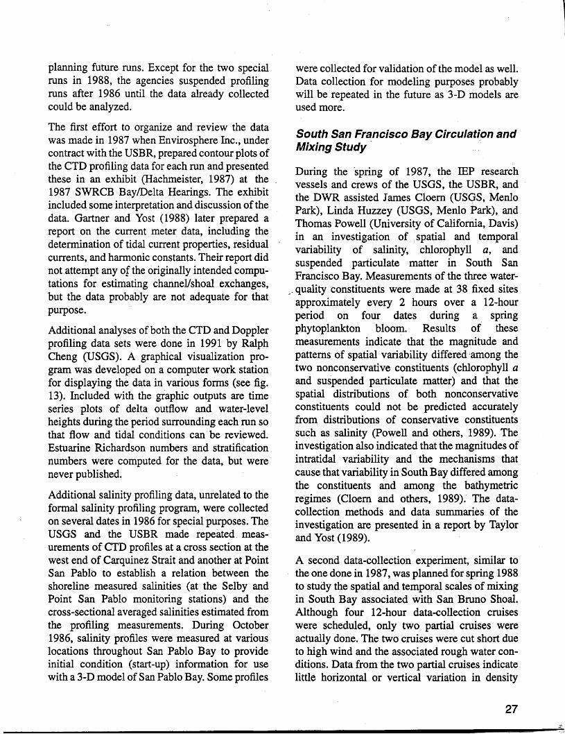
planning future runs. Except for the two special runs in 1988, the agencies suspended profiling runs after 1986 until the data already collected could be analyzed.

The first effort to organize and review the data was made in 1987 when Envirosphere Inc., under contract with the USBR, prepared contour plots of the CTD profiling data for each run and presented these in an exhibit (Hachmeister, 1987) at the 1987 SWRCB BaylDelta Hearings. The exhibit included some interpretation and discussion of the data. Gartner and Yost (1988) later prepared a report on the current meter data, including the determination of tidal current properties, residual currents, and harmonic constants. Their report did notattempt any of the originally intended compu­tations for estimating channel/shoal exchanges, but the data probably are not adequate for that purpose.

Additional analyses of both the CTD and Doppler profiling data sets were done in 1991 by Ralph Cheng (USGS). A graphical visualization pro­gram was developed on a computer work station for displaying the data in various forms (see fig. 13). Included with the graphic outputs are time series plots of delta outflow and water-level heights during the period surrounding each run so that flow and tidal conditions can be reviewed. Estuarine Richardson numbers and stratification numbers were computed for the data, but were never published.

Additional salinity profiling data, unrelated to the formal salinity profiling program, were collected on several dates in 1986 for special purposes. The USGS and the USBR made repeated meas­urements of CTD profiles at a cross section at the west end of Carquinez Strait and another at Point San Pablo to establish a relation between the shoreline measured salinities (at the Selby and Point San Pablo monitoring stations) and the cross-sectional averaged salinities estimated from the profiling measurements. During October 1986, salinity profiles were measured at various locations throughout San Pablo Bay to provide initial condition (start-up) information for use with a 3-D model of San Pablo Bay. Some profiles

were collected for validation of the model as well. Data collection for modeling purposes probably will be repeated in the future as 3-D models are used more.

South San Francisco Bay Circulation and MiXing Study'

During the spring of 1987, the IEP research vessels and crews of the USGS, the USBR, and the DWR assisted James Cloern (USGS, Menlo Park), Linda Huzzey (USGS, Menlo Park), and Thomas Powell (University of California, Davis) in an investigation of spatial and temporal variability of salinity, chlorophyll a, and suspended particulate matter in South San Francisco Bay. Measurements of the three water­

"quality constituents were made at 38 fixed sites approximately every 2 hours over a 12-hour period on four dates during a spring phytoplankton .bloom. Results of these measurements indicate that the magnitude and patterns of spatial variability differed among the two nonconservative constituents (chlorophyll a and suspended particulate matter) and that the spatial distributions of both nonconservative constituents could not be predicted accurately from distributions of conservative constituents such as salinity (Powell and others, 1989). The investigation also indicated that the magnitudes of intratidal variability and the mechanisms that cause that variability in South Bay differed among the constituents and among the bathymetric regimes (Cloern and others, 1989). The data­collection methods and data summaries of the investigation are presented in a report by Taylor and Yost (1989).

A second data-collection experiment, similar to the one done in 1987, was planned for spring 1988 to study the spatial and temporal scales of mixing in South Bay associated with San Bruno Shoal. Although four 12-hour data-collection cruises were scheduled, only two. partial cruises were actually done. The two cruises were cut short due to high wind and the associated rough water con­ditions. Data from the two partial cruises indicate little horizontal or vertical variation in density

27

Benicia Sr.I\) GoldenGate Gr. , IGlullPl, liburon PlnOle Point ' . . ~ . \GarQUinez Sr. IChiPPS 'i~~~1h ofSan JoaqUin ' '' · · · · · PR&,~~.;;' · :=·1I

Color Map M.u: 35.00Min: 0.00

l~:mum tIlItl ~~mum I,· I I

25

-.

t Rip'" MOU!e .. Pan f Mlddlc Mou$C =Zoomr;:B·iU__. I

•.

' l.: '~ · '. ' ."· ·.· :.: .· ,: · ··.··..··..:.· :.·.:··.·.··:..· :.'.....•... ..::: ..:::.'..:: '::.:::,..•.·.·., ·.'·".·,1.'.··.'..'.'·.·.·.··.·.·.····.·.:· ,..:, ,' :: : ' ..:..:..i :..:•....··.··..'·.·.· ··,·.···.·.'.·.· .1•• Salinily [i] ' . 1\ut)jd.

1 1="~~.n ~~·-l i 'I II ' .: Node Discn:lC: V.. -­ <ok< I ':1 Discn:lC _II_ Coolio. I .•. Gra)'Map . Color

!I sros _II_ GRID I ' : . :. : : .: :' ' . ••• • • • b •• • ' ••:. ," '~ . , ' ,:. :::: : : : : : : : : : :

15

..,.. ::~:.: : r:: : ::,=. :.::; :·:~ : .:: ..: :;,,; ,:;.~::: ,: . · '..,..,. :.,:. ':'::... ::::;:-_.'i. LI",. = = = = = = "-"===

TIDES AT THE GOLDEN GATE BRIDGE

5

1.0 0.5 0.0 -h I " If \ f I\ I \ (\ I -0.5 \ I \ J \ } \ I

r ·1.0 ~ ·1.5

" E".,,,.±'i·.,,. , ±'i,,., ., '~,.,,. ,,....,,,. "V"""'_,,;".'M~'.'.,,.,.,.,.,.....Nov 86

Della Outflow =10609 cfs on 10-16-86

Mav86

200000

Nov 8S

0, cfs 240000

HYDROGRAPH

....u.!&:pe; i

~

. . Figure 13 . E~MPLE OUTPUT FROM DISPLAY PROGRAM FOR CONDUCTIVITY-TEMPERATURE-DEPTH PROFILING-RUN DATA.

throughout the area sampled. Based on that finding, and because delta outflow to San Francisco Bay remained very low throughout the study period, the remaining two scheduled cruises were cancelled.

Benicia Sediment StUdy

During March 1990, the hydrodynamic study team participated in a field study of cohesive sedi­ment transport near the eastern end ofCarquinez Strait. The study was a joint effort between Eric Wolanski and his colleagues from the Australian Institute of Marine Science and Ralph Cheng (USGS).

The IEP involvement in the study included the deployment from-March 14 to April-11, 1990, of an upward-looking ADCP and three arrays of two current meters each in a cross section approx­imately 03 km east of the Benicia Bridge crossing of Carquinez Strait. The three current-meter arrays were fairly evenly spaced across the channel, with the ADCP located between the northern and center channel arrays. The ADCP operated well throughout the period, but three of the six current meters failed to provide usable data. The ADCP and current-meter data are pre­sented in a report by J.W. Gartner (USGS, written commun.,1994). Several moving-boat flow meas­urements using the ADDMS were made during the study in an attempt to correlate the measured tidal flows with the measured velocities from the ADCP and current meters. The correlation was never made because of the missing current meter data. The measured tidal flows ranged from -a maximum ebbflow of 16,700 m3/s (590,000 ft3/s)

3/sto a maximum floodflow of 14,200 m(500,000 ft3/s).

More than 30 suspended-sediment profiles, each typically consisting of 7 or 8 suspended-sediment samples, also were collected by the ffiP 'study team at the location of the deployed ADCP. The data were used to develop a correlation between the amplitude of backscattered sound recorded by the ADCP and suspended-sediment concentra­tion. A reasonable correlation for the limited data'

set was obtained. However, the correlation needs further improvement and validation at otherloca­tions in San Francisco Bay. The goal is to use an ADCP for continuous monitoring of suspended­sediment profiles for lengthy periods.

The Australian scientists deployed several erosion sensors on the channel bottom, but these sensors did not function correctly. They also deployed a vertical string of six nephelometers near the location of the ADCP. The nephelometer data confirmed a trend, also indicated by, the suspended-sediment profiles, that the highest 'daily concentrations occurred- near the bottom during floodtides, with, the maximum daily con­centrations occurring during floodflows of spring tides. Because the magnitude of the bottom velocities was less during floodtides than during

" ebbtides, the concentration gradient cannot be related directly to tractive force along the bottom, but probably is related to gravitational circulation and the presence of the entrapment zone.

The Australian scientists also collected a 25-hour set of CTD profiles with an instrument equipped with a nephelometer. Profiles were taken at 9 to 10 locations across the channel at hourly intervals during a complete tidal cycle. The data set was collected to investigate the -variability of suspended-sediment concentrations across, the channel throughout a tidal cycle. Analysis of the data collected during this study has not been completed by the Australian scientists or the USGS.

-,

Carquinez Strait Study

From December 6", 1990, to April 18, 1991, the IEP study team collected data at Carquinez Strait. The purposes of the data collection were to:

1. Obtain data for verifying 3-D models of the strait;

2. Measure the variation in magnitude of gravi­tational circulation in the strait relating to the spring-neap tidal cycle;

3. Measure the magnitude, of tidal flows in the strait using the ADDMS;

29

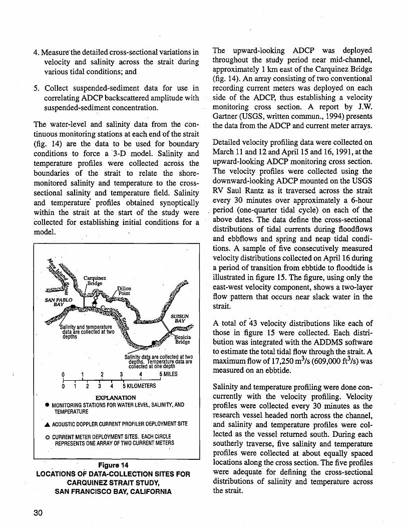
4. Measurethe detailed cross-sectional variations in velocity and salinity across the strait during various tidal conditions; and

5. Collect suspended-sediment data for use in correlating ADCP backscattered amplitude with suspended-sediment concentration.

The water-level and salinity data from the con­tinuous monitoring stations at each end <of the strait (fig. 14) are the data to be used for boundary conditions to force a ',3-D model. Salinity and temperature profiles were collected across the boundaries of the strait to relate the shore­monitored salinity and temperature to the cross­sectional salinity and temperature field. Salinity and temperature" profiles, obtained synoptically within the strait at the start of the study were collected for establishing initial conditions for a model.

o 2 I I

i . i !

I o 234 5KILOMETERS

EXPLANATION • MONITORING STATIONS FOR WATER LEVEL, SALINITY, AND

TEMPERATURE

.A ACOUSTIC DOPPLER CURRENT PROFILER DEPLOYMENT SITE

o ,CURRENT METER DEPLOYMENT SITES. EACH CIRCLE REPRESENTS ONE ARRAY OF TWO CURRENT METERS

Salinitv data are collected attwo depths. Temperature data are collected atone depth

3 4 5 MILES I ,

Figure 14 . . LOCATIONS OF DATA-COLLECTION SITES FOR

CARQUINEZ STRAIT STUDY, SAN FRANCISCO BAY, CALIFORNIA

The upward-looking ADCP was deployed throughout the study period near mid-channel, approximately 1 km east of the Carquinez Bridge (fig. 14). An array' consisting of two conventional recording current meters was deployed on each side of the ADCP, thus establishing a velocity monitoring cross section. A report by 1.w. Gartner (USGS, written commun., 1994) presents the data from the ADCP and current meter arrays.

Detailed velocity profiling data were collected on March 11 and 12 and April 15 and 16, 1991, at the upward-looking ADCP monitoring cross section. The velocity profiles were collected using the downward-looking ADCP mounted on the USGS RV Saul Rantz as it traversed across the strait every 30 minutes over approximately a 6-hour

"period (one-quarter tidal cycle) on 'each of the above dates. The data define the cross-sectional distributions of tidal currents during floodflows and ebbflows and spring and neap tidal condi­tions. A sample of five consecutively measured velocity distributions collected on April 16 during a period of transition from ebbtide to floodtide is illustrated in figure 15. The figure, using only the east-west velocity component, shows a two-layer flow pattern that occurs near slack water in the strait.

A total of 43 velocity distributions like each of those in figure 15 were collected. Each distrl­bution was integrated with the ADDMS software to estimate the total tidal flow through the strait. A maximum flow of 17,250 m3/s (609,000 ft3/s) was measured on an ebbtide.

Salinity and temperature profiling were done con­currently with the velocity profiling. Velocity profiles were collected every 30 minutes as the research vessel headed north across the channel, 'and salinity and temperature profiles were col­lected as the vessel returned south. During each southerly traverse, five salinity and temperature profiles were collected at about equally spaced locations along the cross section. The five profiles were adequate' for defining the cross-sectional distributions of salinity and temperature across the strait.

30

~ 0

l~!!~~~11= 20 ~ Y fu 25 TIME =10:03 Cl DISCHARGE =9,300 CUBIC METERS PER SECOND . .

u! - 40--- 30 - 20- 10 :;.:~ -:""I -- -;-:::-=:. • - ­__ .30 ~20 r: r--;::----~.10-~.

-:::. 20----:-:"10· - - -~_ .. -' . .. 1= 20 fu 25 TIME =10:49 Cl DISCHARGE =2,300 CUBIC METERS PER SECOND

I:i:i 5 ffi o~:iE 10 ~. 15 1= 20 TIME;" 11 :32fu 25 Cl DISCHARGE =-5,000 CUBIC METERS PER SECOND

o......--.....J o 125 DISTANCE INMETERS

SHADING INDICATES AREA OF NEGATIVE (EASTWARD) VELOCITIES. CONTOURS OF VELOCITY IN CUBIC METERS PER SECOND.

Figure 15 VELOCITY DISTRIBUTIONS AND FLOWS (Q) IN

CARQUINEZ STRAIT, SAN FRANCISCO BAY, CALIFORNIA.

Positive velocities and flows are westward. (modified from Smith, 1994.)

Several vessel cruises were made for purposes of depth sounding. The soundings revealed sand dunes were present in the strait and ranged from approximately 0.3 to 5 m in height. The largest dunes were in the deepest water of the strait (35 m) just south of Dillon Point (fig; 14). The location for deploying the upward-looking ADCP was carefully selected in an area of the strait where the dunes were small and little dune move­ment was observed. Despite this precaution, in April 1991, the ADCP was buried under sand. After considerable effort, the unit was retrieved

without sustaining damage, but no data were recorded after March 27 when the transducer head apparently became covered with sand. During April 1991, 14 suspended-sediment profiles, con­sisting of 7 samples each, were collected at the ADCP deployment site for use in calibrating the amplitude of ADCP backscattered sound with suspended-sediment concentration. Because these profiles were collected during the time that the ADCP was buried, calibration could not be attempted.

Data from this study were reduced and organized into computer files for use as a test case for verifying 3-D hydrodynamic models (Smith and others, 1992; Smith, 1994). The detailed distri­

' butions of velocity, salinity, ' and temperature across the strait, combined with the 4 months of continuous measurement of velocity profiles with the upward-looking ADCP, represent one of the most complete data sets for 3-D model veri­fication ever assembled. The data are available in graphical and digital .form on request to the USGS and are being disseminated by the Computational Hydraulics Committee of the American Society of Civil Engineers. It is hoped that several inde­pendent 3-D modelers will begin applying their models to the data set beginning sometime in 1996. The IEP study team plans to oversee model applications to the strait and to incorporate attractive features of the various 3-D models into the new USGS 3-D model.

Measurement of Delta Outflow into San Francisco Bay

As mentioned earlier, the net or tidally averaged flow'into San Francisco Bay from the delta (delta outflow) is not measured directly, but is estimated by a calculation procedure known as DAYFLOW (California Department of Water .Resources, 1986). During spring 1988, two identical experi­ments were carried out to demonstrate the capability of the ADDMS for measuring net delta outflow. The measured outflows were then compared with the outflows estimated by using DAYFLOW.

31

For each experiment, the ADDMS measured tidal flow every 15 minutes across the channel south of Chipps Island (fig. 2) during a 25-hour period (one complete tidal cycle). Each individual tidal-flow measurement required from 6 to 8 minutes to complete depending on the wind and surface-wave conditions that existed when crossing the l-km­wide channel. To obtain the net flow, tidal flows were integrated over the tidal cycle. The first experiment was conducted April 27-28, 1988, on a neap tide and the second May 5-6, 1988, on a spring. tide.

Plots of the 'two sets of tidal flow measurements are shown in figure 16. Tidal flows at Chipps Island

~~ 10 ,., NET DISCHARGE =110=> en 8Ow ~ :" CUBIC METERS PER Z::E 6 ~ •., : t)g SECOND (3,900 CUBIC ~_~ 0 D ° ~ FEET PER SECOND)C!Jc,4 ... 0 0 00::2 2· 0' o • 0

~§ '0 : • o•5!2 ~ -2 ' o. .0 o

C UJ .4 ~ 0 0 o 0 Cl C. •• o 0

~ en .6 ~ ..: • 0

~o:: V~ ~ -8 ~ NEAP TIOE ~. 00::: ~ ·10 0 2..::: 5 10 15 20 5 30

TIME. IN HOURS FROM 1400, APRIL 27. 1988

10 ,,.,,,,,...... NET DISCHARGE =200 CUBIC METERS PER SECOND

8 to : -..- (7,100 CUBIC FEET PER SECOND) o 4IlI6

4 to: ... ,~ .2 ~. : ! .... •

o ·2 ,.

•

•••0 ..

• • • I···4 • • . ,.

·6 to 4\ , •., • •\ . SPRING TIOE .~,.. Y .

5 10 15 20 25 TIME. IN HOURS FROM 0600. MAY 5.1988

Figure 16

DISCHARGES MEASUREDBY THE ACOUSTiC

DOPPLER DISCHARGE MEASUREMENT SYST~M

(ADDMS)AT CHIPPSISLAND, SAN FRANCISCO BAY, CALIFORNIA.

Positive flows are downestuary (westward). Netvaluesare determined by integration over the tidal cycle.

were large, with peak flows exceeding 8,500 m3/s

(300,000 ft3/s). The net flows were calculated to be 110 m3/s (3,900 ft3/s) on the neap tide and 200

3/s,m (7,100 ft3/s) on the spring tide. For comparison, the DA,YFLOW estimates during the period from Apri122 (day 113) to May 9 (day 130) are shown in figure 17 with the ADDMS measurements superimposed..The measured flow was less than the DAYFLOW estimate on the neap tide and greater than the DAYFLOW esti­mate on the spring' tide. These results were expected because the, DAYFLOW calculation, which is based on an upstream mass balance, does not include any variability in the net flow resulting from the spring-neap tidal .cycle, Current meas­urements and numerical model calculations made

, farther seaward in San Francisco Bay indicate that, because of tidal effects, net flows in the bay are greater during spring tides than during neap tides and can sometimes tum .landward during neap tides.

C 700 r--..,.---,--r-r--....--~--r---.....-,.-, 2

~§ 600 0:: en ~ 0:: 500 o~ 5!2 en 400Co::

~ ~ 300 Ld~eQ 200 w al

25100 ~ 0 L-~--L.-~_I...-""'----l-.---L...----L_.L.-......J

112 114 116 118 120 122 124 126 128 130 132 DAYS FROM JANUARY 1.'1988

Figure 17

DAYFLOW ESTIMATES OF NET DELTA DISCHARGE AND INTEGRATED ACOUSTIC

DOPPLER DISCHARGE MEASUREMENT SYSTEM (ADDMS)MEASUREMENTS AT CHIPPS ISLAND,

SAN FRANCISCO BAY, CALIFORNIA. Arrowheads markthedayswith theweakestneapand

the strongest springtides during the period.

32

Deployments of Upward-Looking Acoustic Doppler Current Profilers

Between 1988 and 1992, the upward-looking ADCP was deployed.· four times. Those deployments are described below.

Carquinez Strait, March-November 1988

The first deployment of the upward-looking ADCP was made on" March 25, 1988, at the western end of Carquinez Strait about 180 m from the south bank of the channel at a depth of 16.8 m below mean lower low water (MLLW). Each measured velocity profile was defined by 12 data points spaced at l-m intervals (bins) over the water column. The first measurement point (bin 1) was centered at .a distance of 2.1 m above. the estuary bottom and the uppermost point (bin 12) at a distance of 14.1 m above the bottom, or 2.7 m below the. water surface at MLLW. The data-collection cycle was set at.lfl minutes. After about 7 months of continuous data collection, the instrument was retrieved on November 4,1988.

The ADCP profiles were separated into time series of two horizontal velocity components for each bin, north and east, and were used for pres­entation and analyses of results, including plotting, tidal harmonic analysis, and computation of residual currents (Burau and others, 1993). The four most significant astronomical tidal constit­uents identified were the semidiurnal and diurnal components M2, S2' Kb and 01' These compo­nents have been identified as dominant in many previous analyses of tide and tidal 'current measurements in San Francisco Bay (Cheng and Gartner, 1984). Residual currents were computed by applying a digital, low-pass' filter to the tidal current time series of each bin.

The shifting in and out of phase of the semidiurnal and diurnal tidal constituents (sometimes referred to as "beating") modifies the magnitude of tidal currents in Carquinez Strait by as much as a factor ' of two during a typical 14-day spring-neap cycle. Walters and Gartner (1985) and Walters and others (1985) previously examined ·the effect of the spring-neap cycle on density-driven

gravitational circulation in San Francisco Bay by analyzing subtidal variations in currents from measurements made using conventional current meters. The high resolution, residual current profiles obtained with the ADCP in 1988 provided a much more detailed .measurement of this phenomena in San Francisco Bay and served to substantiate earlier findings.

Nontidal .currents from five" of the .ADCP bins measured during May 1988 are shown in figure 18. A graph of tide heights is included to

.assist in identifying the spring and neap tides. The relation between the density-current speed and the tidal energy is apparent, particularly in the lower layers 'of the water column. During neap tides when vertical mixing is relatively small, the flow reverses along the bottom and maximum land-:

" ward currents are about 8 to 10 crn/s. During spring tides when vertical mixing is greater, the currents are seaward over the entire depth of flow and the overall vertical shear in the profile is con­siderably less than during neap tides. During the deployment period, the variability in delta outflow to SanFrancisco Bay was small, so changes in the magnitude of the gravitational circulation are not attributable' to 'outflow variations. Data from this ADCPdeployment is also discussed in a paper by Smith and others (1991).

Carquinez Strait, March-April 1990

From March 14 to Aprill1, 1990, the ADCP was" . deployed near the east end of Carquinez Strait near Benicia as partof the sediment study that was described previously. The depth of water at the ' deployment sitewas about 15 m. Data from this deployment and two others mentioned below are given. in a report by J.W. Gartner (USGS, written commun., 1994). The report includes' plots of tidal. current speed and -direction for each ADCP bin, results of tidal harmonic analysis, plots of residual . currents, .and other information. No additional analyses of these data have been done. It is expected, however, that all of the ADCP data will be used in calibrating a 3-D model of the entire bay. .

33

10 .-----------------------------, UP BIN 10 NEAR SURFACE

o

-20 L- ---'.u..w.__.....:.:..:....__-,-__~

·20 ~===============================~==================-'__,

+ ESTUARY

-10 t DOWN

10

o

CI -10 z o o

~ a: 10 w Q..

ena: o ~ ~ i=ffi -10 o z >_-. -20t; 10 ...-----------~-----------------,

BIN 4 ~ >

-10

-20 ~==========================================~10 ..... BIN 2

o 1II1111Vll""' ·"',VI'\\IIIIII!II~llllffI~llll$ff!.L\\,',-",IQ/IIIWIVUllffl/llIIb'r'l

-10

NEAR BOnOM

122 124 126 128 130 132 134 136 138 140 142 154 DAYS FROM JANUARY 1,1988

.Figure 18

FIVE BINS OF LOW-PASS FILTERED CURRENTS FROM THE ACOUSTIC DOPPLER CURRENT PROFILER (ADCP) DEPLOYED IN CARQUINEZ STRAIT, SAN FRANCISCO BAY, CALIFORNIA.

(Modified from Smith and others, 1991.)

'", .... 34

San Pablo Bay, October-November 1990

From October 19 to November' 29, 1990, the ADCP was deployed in San Pablo.Bay and col­lected data to be used in verifying a 3-D model. The ADCP was just northwest of the deep water channel and approximately 3 km northwest of Pinole Point. Depth of the water at the. site was about 12 m.

Carquinez Strait, December 1990-June 1991

From December 6, 1990, to June 5, 1991, the ADCP was deployed in Carquinez Strait as part of the study described previously. No data was recorded after March 27 because the transducer head was covered with sand.

35

.' ;

Chapter 3 MODELING ACTIVITIES

Because hydrodynamic field measurements in estuaries are difficult and expensive to do, obtaining measurements dense enough in time and space to provide an adequate description of the circulation and mixing processes usually is not possible. This is especially true for San Francisco Bay where the greatest need is for information on tidally averaged hydrodynamic quantities, which would require continuous data collection during several complete tidal cycles. An alternative to field studies is mathematical modeling studies, which can be particularly useful for deriving dis­tributions of tidally averaged quantities. Modeling studies alone, however, are of little value if they are not adequately verified with field meas­urements. For these reasons, the hydrodynamic study was designed as an integrated program with both mathematical modeling and field meas­urement activities. Field measurements are used for boundary and initial conditions for mathe­matical models and for model calibration and verification. In this chapter, the activities related to the modeling part of the study are discussed and reviewed.

The choice of models and modeling tasks in the hydrodynamic study were influenced by the avail­ability of computer resources. Even with today's sophisticated computers, the computing require­ments for time-varying 2-D and 3-D circulation models are considerable, depending on the spatial grid size, the time step size, and the length of the simulations. For San Francisco Bay, the spatial grid size of the model must be kept small to resolve the bathymetry. The 1- to 2,;,km-wide deep-water channels can be resolved only with grids of0.25-km resolution or less. This small size of the horizontal grid imposes a limitation (called the Courant condition) on the maximum time step allowable for a model to obtain stable and accu­rate solutions. The time-step limitation is greatest where the water is deepest, so Central Bay, with depths exceeding 100 m near the Golden Gate, often becomes a controlling area. In addition,

because many of the biological processes, as well as delta outflows, vary over seasonal and longer time periods, hydrodynamic simulations must be

. made for periods of 3 to 6 months or longer. Therefore, computing times can become lengthy when models are configured to the' entire bay, which would require more than 200,000 (2-D) nodes. When there are a large number of nodes, the size of the central processing memory and disk storage of a computer is an important issue.

Since the start of the hydrodynamic study, the computers used by the modeling team have been upgraded almost every year; the "in-house" com­

.: puters presently (1995) used are more than an order of magnitude faster' than the ones used in 1984. Advances in computer networking allow near easy access to supercomputers that offer even greater speedups in computing times when. needed, especially for large models and long sim­ulations. Advances in the programming and design of numerical software used in hydro­dynamic codes account for an additional 10-fold or more speedup in model run times. The combin­ation of faster computers and, more efficient models now allows much larger and longer model simulations to be done. Whole-bay 2-D sim­ulations with fine grids are accomplished easily on the latest workstations, and whole-bay, 3-D simulations are feasible for the first time. In the early years of the study, the first 2-D model appli­cation was confined to Suisun Bay because of the computing time required, and the first 3-D model simulations for San Pablo Bay could not be accomplished in real time using a course grid and only. a few vertical layers. If improvements in modeling capabilities continue into the future at the same rate as in the recent past, computer requirements will become a much less limiting factor in modeling studies.

Despite an increasing trend in the number of hy­drodynamic modeling studies being done in other estuaries worldwide, there are still relatively few . computer codes available for multi-dimensional

37

modeling. These codes require extended periods of time for development and testing by a team of individuals experienced in modeling, hydrody­namics, and applied mathematics. Few organiza­tions are willing to support these efforts. Most codes that are available were not developed by public agencies, but rather were developed by consultants and universities. Consultant codes usually are proprietary and, therefore, can be obtained only through contract. University codes are primarily the product of research studies and

. generally are not tested or documented suffici­ently for practical applications. Out of necessity, the IEP modeling team developed several "in­house" codes for use in the modeling studies. A new one-dimensional (I-D) delta model and two 2-D models were-programmed almost entirely by the modeling team. Two other 2-D codes used in the study were programmed by the USGS in Menlo Park in collaboration with others, yet some reprogramming and considerable testing of these codes were still required by the IEp· modeling team. Two of the 3-D codes used or tested by the modeling team were obtained through contracts with consultants. A third 3-D code was evaluated for possible future use and is now being further modified' and developed at the University of Trento, Italy. Each of the 2-D and 3-D codes used in the study are discussed below.

One additional issue related to modeling involves the graphical presentation of results. Individual runs of a multidimensional model can easily gen­erate outputs with millions of numbers on time­varying velocities, tidal heights, salinities, and other variables for an estuary. The only way to interpret and analyze these outputs is to use computer graphics. Although only passing mention' of computer graphics is made in this report, developing graphics programs has been a major part of the study and the modeling team has kept abreast of the latest advances in this field. Techniques of scientific visualization are being used to animate time-varying outputs from 2-D and 3-D models. Scientific visualization is a rela­tively new field in computer science and, because of theincreased.availability of relatively low cost scientific workstations with advanced graphics

capabilities, is quite popular. The trend toward scientific visualization is accelerating and will receive increased attention in modeling studies in the years ahead. ­

Two-Dimensional Modeling in the Horizontal Plane

Work tasks involving 2-D models in the hori­zontal plane are reviewed in this section. These models also are referred to as vertically averaged, or x-y models, and solve for the hydrodynamic variables of velocity and salinity as averages over the depth of flow in the' estuary. Vertically averaged models are useful for 'examining the horizontal variation in hydrodynamic variables, but not the vertical variation. These models are to

" be distinguished from 2-D models in'the vertical plane, which are discussed in a later section. A

.limitation of x-y models is that they assume conditions in the estuary are well mixed vertically, which requires that salinity stratification be weak or absent. For San Francisco Bay, these models are most appropriate during periods of low delta outflow. This section is organized around the three 2-D, vertically averaged models that have been used in the hydrodynamic study.

Alternat~ng-Direction-/mplicit Model

The first 2-D model applied by the modeling team was a version of the well known alternating: direction-implicit (ADD, finite-difference model originally described in a report by Leendertse and Gritton (1971). The model was first used in the hydrodynamic study of Suisun Bay by Smith and Cheng (1987). For their application, the model was modified to include, a horizontal, density­gradient (baroclinic), forcing term because of the appreciable horizontal salinity gradients in Suisun Bay. A new solution scheme for the salt-transport equation also was added to the code using the techniques described by Cheng and Casulli (1982). Further details on the numerics in the model are included in the report by Smith and Cheng (1987).

. ,

Suisun B'ay was chosen for study because it is biologically important and because circulation in

this area is affected significantly by delta outflow. The shallow depth of Suisun Bay also makes it more suited for a 2-D analysis than San Pablo or Central Bays where 3-D effects are more dominant. A low-flow summer period was selec­ted for study because 3-D effects at low flows are less important. The boundaries of the modeling study were limited to Suisun Bay because of prac­tical considerations related to the computing time requirements of the model.

The objectives of the Suisun Bay application were first to calibrate and verify the model with sea­level and current-meter data and then to use the model to study the effects of tides, wind, and salinity gradients on tidal and residual circulations during a low-flow summer period. These objectives generally were met.

The model was configured with the finest grid size (0.25 km) that could be run economically with the computer resources available. The depths at 4,500 nodal points were taken from available navigation charts. To verify the input bathymetry, depth contours were drawn and compared with contours on the navigation charts.

Available salinity data for the areas near the' model boundaries at Chipps Island and Carquinez Strait were used to estimate salinity boundary conditions that were consistent with summer conditions. Over a period of several weeks, salinity could be approximated as a sum of sine functions with the same frequencies as the tidal currents; the salinity maxima and minima were assigned at high and low slack water, respectively. This approximation for salinity implies that tidal variations of salinity are dominated by the seaward-landward advection of salt rather than by tidal diffusion. This salinity boundary condition was used for all hypothetical simulations.

November 1979 and November 1980 were selected as the independent periods for the cali­bration and verification of the model because sea­level and current-meter data were available for those periods from a report by Cheng and Gartner (1984). The location of the data stations are shown on figure 19. During calibration, the model

predictions were adjusted by altering the bottom friction and horizontal eddy viscosity coefficients until sea-level and .current predictions best matched the data. Sea-level predictions were close to perfect, whereas velocity predictions had some noticeable differences (fig. 20).. These differences were attributed to three factors:

• The model grid was too coarse to represent the bottom topography in some areas;

• The estimates of delta outflow used to adjust the simulated net flows through Suisun Bay were not accurate enough for modeling pur­poses and did not reflect variation in net flows due to the spring-neap tidal cycle; and

• The measured currents at a single point in the water column obtained from moored current meters could not be compared properly with the vertically averaged currents simulated by the model.

A fourth factor to explain the differences could be the use of a numerical technique called upwinding in the simulations, which was necessary because of the coarse model grid. The use of upwind­weighted finite differences to represent deri­vatives in the governing partial-differential equations can introduce too much artificial visco­sity, or smoothing, in a numerical solution. This artificial smoothing can reduce the gradients of velocities between the channels and shallows and, in particular, can reduce the predicted velocities in the channels at some current-meter sites. Because of these concerns, the grid was eventually refined and the upwind differencing procedure was changed in the AnI model.

This model application demonstrated the effects of salinity (density) gradients and wind on net flow through Suisun Bay. By omitting either density-gradient or wind forcing from the simu­lations, net flow through the bay was changed by as much as an order ofmagnitude (fig. 21). Proper simulations of residence time and residual currents also were dependent on the quality of the sea-level, salinity, and wind data input to the model. To include density forcing in a model, the hydrodynamic and salt-transport equations must

39

o ~

122010' 1220 121°50'

EXPLANATION • CURRENT METER STATION

38°10' £. STAGE STATION

• U.S. GEOLOGICAL SURVEY WEATHER STATION

-2- BATHYMETRIC CONTOUR-­Interval 2meters. Datum is mean lower low water ..

38°05'

·:.. ··:.... ..,.~:.... .:.~

·~11 38°

Figure 19

LOCATIONS OF CURRENT-METER AND WATER-LEVEL STATIONS USED IN CALIBRATION AND VALIDATION OF THE SUISUN BAY, CALIFORNIA, TWO-DIMENSIONAL MODEL. STATION NUMBERS ARE THOSE OF CHENG AND GARTNER (1984). ALSO SHOWN IS THE

LOCATION OF THE U.S. GEOLOGICAL SURVEY WEATHER STATION AT WHICH WIND DATA WERE COLLECTED.

(Modified from Smith and Cheng, 1987.)

(A)

1600 2200 0400

100

o 1000

Station C29

Ebb Flood Flood Ebb

1600 2200 0400 1000 1600 2200

Stat ion C30

0400 1000

!! ! l'I Flood

:! ," \

Ebb Flood

NOVEMBER 2-3, 1979

o 0700 1300

Stat ion C237

,..,.::.==......" Ebb Ebb ;

I ~

I 1900 0100 0700 1300 1900 0100 0700

(B)

Flood Ebb

1300 1900 0100

NOVEMBER 11-12. 1980

Figure 20

CURRENT SPEEDS ANDDIRECTIONS OBTAINED DURING (A) CALIBRATION AND(B) VALIDATION OFTHE SUISUN BAY, CALIFORNIA, TWO-DIMENSIONAL MODEL.

(Modified from Smith and Cheng, .1987.)

41"

5,000 .----..----~...---r-...,--,r--r--r---r---____,

4,000 SIMULATION o WITHOUT SALlNllY GRADIENTS OR WIND

~ 3,000 • WITH WIND, BUT WITHOUT SALINllY GRADIENTS o o WITH SAlINllYGRADIENTS, BUT WITHOUT WINDu UJ

o~ 2,000 UJ a.. en •ex: UJ

tu o 0 ~ 1,000 u a:i 800::::J U

~ 600 • ~ 500 a: ~ 400 uB. 300 o «!3 • 0~ 200 otu z

100 1....-~-...L...-_.L--.....l...-.....L.-....J......Jl.-...I-..L-L..__----l

1 2 . 3 4 5 6 8 10 20 FALL IN MEAN WATER lEVEL ACROSS SUISUN BAY,

IN CENTIMETERS

Figure 21

NET (TIDALLY AVERAGED) DELTA OUTFLOW AT

CHIPPS ISLAND COMPUTED FROM SIMULATIONS . .

AS A FUNCTION OF THE FALL IN MEAN WATER

LEVEL ACROSS SUISUN BAY, CALIFORNIA.

be coupled to each other by including the density­gradient term in the hydrodynamic momentum equations. Previous models.of San Francisco Bay had neglected this term.

Spectral Model

The first 2-D model of the entire San Francisco Bay was a finite-element, spectral model described in reports by Burau and Cheng (1988; 1989a). This model was programmed entirely by the modeling team during the first few years of the study. A spectral model was chosen because long-term simulations are" more economical than those done with traditional time-stepping models, such as the

ADI model discussed above. At the time development of the spectral model, began, applying a time-stepping model to the entire S~

Francisco Bay was not considered feasible.

A spectral model differs in concept from a time­stepping model. The spectral model assumes that water levels and velocities can be represented by a summation of harmonic (normally cosine) func­tions, called tidal constituents (fig. 22), each of which has a particular amplitude, frequency, and phase angle. The amplitude and phase angle of each constituent are unknowns and must be solved at each nodal point of the numerical grid; the frequencies are astronomical constants that are known. In the physical system, the amplitudes and phase angle of each tidal constituent are modified, primarily by friction and basin geometry, as a tide

-: wave propagates through an estuary (fig. 23). Because predictions of tideheights and velocities made using a spectral model involve only the evaluation of simple harmonic functions, long­term simulations are very economical.

The spectral model forSan Francisco Bay is based on a, linearized form of the 2~D governing equations that are described by Burau and Cheng (1989a). These equations contain, two unknowns-the tide height and the tidal velocity vector-s-that vary with location and time. When linearizing the equations, various terms in the governing equations are either neglected or linearized. The model does not, therefore, include all the physics contained in a fully nonlinear model. A limiting assumption in the spectral model for San Francisco Bay is that the density­gradient forcing is neglected. The ADI model study in Suisun Bay identified this term as i~portant under most conditions.

Before solving the governing equations, the time variable in the spectral model is eliminated by substituting harmonic functions" for the unknown tides and tidal velocities. The numerical solution is then performed using the standard Galerkin finite-element procedure. The horizontal grid uses simple triangle-shaped' elements. After' imposing shoreline and open-water boundary conditions,

42

--,

Spring FIELD DATA

+1

o

Neap

·1

o

ena: w

~ 0

o

o

o

o

o

o

o v·2

10 20 30 31

JANUARY, 1980

Figure 22

TIDAL ELEVATIONS AT THE GOLDEN GATE, SAN FRANCISCO BAY, CALIFORNIA, ESTIMATED FOR JANUARY 1980 (MODIFIED FROM CHENG AND GARTNER, 1984) SHOWING TWO HIGHS AND TWO LOWS

EACH DAY,TWO PERIODS OF SMALL TIDAL AMPLITUDES AROUND THE 10TH AND THE 24TH (NEAP TIDES), AND THREE PERIODS OF LARGE TIDAL AMPLITUDES AROUND THE 1ST, 18TH, AND 30TH (SPRING TIDES).

Thecontribution of the majortidal constituents are shown below the elevations. Thoseconstituents with subscript 2 have twice daily 'frequencies, and thosewith subscript 1 have oncedaily frequencies.

43

TIME DIFFERENCE OF AMPLIFICATION OF HIGH WATER, IN HOURS TIDAL AMPLITUDE

o M2

2 3 0.6 0.8 1.0 1.2 1.4 60

40

20

en 0a:: LU

ti:i :::2: 0 ..J 2052 z w.. e.,:)

Z 40~ en

Q

60

80

DUMBARTON BRIDGE

I,, I,,,

I

",,'..,.. I '

I I I,,,

I

-: \ M2 ' , \ \, I

K1 ~' ,, I

I, ",,"

,,,"

62,

'\ '\

'\ '\ ..

'\ '\

'\ '\

'\ '\

'\ '\

'\ '\

'\ '\

'\ '\

'\ '\

'\ '\

'\

" .. .. " .. .. ..

" .. .. ..........

.....

.------r--.....-----.,.....----r---r-~-__r_1 .-----r----r-~---r----r---r____.____.

100

Figure 23 AMPLIFICATION OF MAJOR DAILY(K1) AND TWICE DAILY(M2) TIDAL CONSTITUENTS AND THE

TIME DIFFERENCE OF HIGHTIDE WITHIN SAN FRANCISCO BAY, CALIFORNIA, IN RELATION TO THE GOLDEN GATE.

(Modified from Walters and others, 1985.)

a set of algebraic equations is solved independ- (Burau and Cheng, 1988). Later, a fine resolution ently for each tidal frequency using computerized grid of approximately 18,000 node points, was matrix solution techniques. Subsequently, time- prepared using bathymetric data retrieved from a varyin.g tides and ~dal velocities ar: computed by computerized data base (described in Chapter 4). summmg the solutions for all 'constituents. The fine-grid model was.calibrated and validated

The spectral model was first calibrated for the for six tidal constituents using a mathematical M2 tidal constituent in 1988 using 'a medium procedure that minimizes the mean-squared error resolution grid (fig.24) of 7,000 node points for each constituent.

Figure 24 FINITE ELEMENT GRID OF SAN FRANCISCO BAY, CALIFORNIA, USED FOR

SPECTRAL MODEL COMPUTATIONS• . (From Burau and Cheng, 1988.)

45

The harmonic constants derived by the spectral model were used for the first complete description of the tides within San Francisco Bay. The solutions by the spectral model have not yet been compared with solutions generated by a nonlinear tidal model. Thus, the applicability of a linear, solution to the shallow-water equations for San Francisco Bay cannot be judged. This question must be answered before further use of the spectral model is attempted.

Tidal, Residual, and Intertidal Mudflat Two-Dimensional Model.

In 1991, the modeling team .began using a new 2-D model called TRIM2D (Tidal, Residual, and Intertidal Mudflat 2,-D Model) that was developed by Vincenzo Casulli of Italy in collaboration with Ralph Cheng of the USGS (Cheng and Others, 1993). TRIM2D is a nonlinear, time-stepping model, like the ADI model, but uses a fully multi­dimensional solution technique instead of the alternating-direction technique used in the ADI model. The advantages of the fully multi­dimensional technique are discussed in the next section. The finite-difference scheme in TRIM2D . is semi-implicit, meaning that only certain terms in the 2-D model equations are treated implicitly (involving more than one unknown variable) and the others are treated explicitly (involving a single unknown variable).

By treating certain key terms implicitly, TRIM2D is not constrained by any stability limitation on the maximum size of the time step, a disadvantage of models that are fully explicit. IIi comparison to a fully implicit model, the size of the system of equations that TRIM2D solves with matrix methods is greatly reduced, which has a large effect on efficiency. In addition, the system of equations solved by TRIM2D are linear, whereas those in a fully implicit model are nonlinear and are difficult and inefficient to solve. For use on San Francisco Bay, the semi-implicit TRIM2D is clearly an improvement in efficiency over either explicit or fully implicit models.

A 6-day simulation of San Francisco Bay with TRIM2D requires about 1 hour of computer time. on a 17 mips (million instructions per second)

46.,

workstation using a IS-minute time step and a O.5-km grid size (Cheng and others, 1993). Thus, seasonal simulations can be accomplished over a weekend. Because the model has been vectorized, it can be run efficiently on supercomputers if that becomes necessary.

Although programming on the equation solving parts of the code was not modified by the modeling team, considerable reprogramming of input and output subroutines was done to make the model more amenable to practical applications. Graphics visualization programs were written to interface with model output. The model also was tested by the modeling team, on several hypothetical problems and was applied to Suisun Bay using a very fine (50-m) grid.

Discussion of Two-Dimensional Models

Of the three 2-D'models discussed above, the ADI model and TRIM2D are similar. Both models are nonlinear, time-stepping, finite-difference models. For future applications that require a non­linear model, TRIM2D will be used instead of the ADI model, primarily because of computational efficiency. For simulations of San Francisco Bay, the fully multidimensional numerical approach employed in TRIM2D is more efficient than the ADI approach. In recent years, researchers have discovered that ADI models suffer from a source of inaccuracy known as the ADIeffect (Stelling and others, 1986). This ADI effect is most significant in flow domains where the bathymetry is complex, especially where one or more narrow channels are not aligned with the principal directions of the numerical grid, and can be eliminated only by decreasing the time step or grid size of a simulation. Modeling of San Francisco Bay has shown that the time step of the ADI model must be kept quite small (S2 minutes) to achieve accurate simulations in Suisun Bay where the geometry and bathymetry of the bay are quite complex. By using TRIM2D, a time step of 15 minutes is possible. The largertime step with TRIM2D'results in about.a five-fold speed-up in the runtime of the model compared with the ADI model.

For future 2-D model applications, a choice remains between the spectral model and TRIM2D. This choice will not always be obvious and can depend on the particular application. For straightforward predictions of tidal heights and velocities, the spectral model is completely ade­quate and probably is preferred. The extremely fine grid used with the spectral model results in a better representation of the bathymetry than does the rectangular grid used with TRIM2D. 'The spectral model, despite its fine grid,' is more efficient computationally for most applications than is TRIM2D. But with today's faster com­puters, nonlinear 2-D models like TRIM2D can be economical to run. When nonlinear effects are important, TRIM2D is the preferred _choice. Nonlinear effects-probably play an important role in predictions of long-term transport, and certain types of eddying patterns and some features of residual circulation cannot _be simulated with a linear model. For these reasons, 'TRIM2D may be required for all simulations ofresidual circulation and long-term transport.

Two-Dimensional Modeling in the Vertical Plane

A 2-D model in the vertical plane is referred to as a laterally averaged or x-z model. This type of model solves equations that are integrated laterally across an estuary (perpendicular to the primary direction of the tidal currents) along layers spaced down through the water column. The model can be used to study vertical variations in hydrodynamic quantities, but not horizontal variations. A laterally averaged model was used in the hydrodynamic study to study vertical varia­tions in horizontal circulation instead of doing full 3-D simulations. Because of the simplified equations and limited number of nodal points, an x-z model is efficient computationally when compared with a full 3-D model.

A laterally averaged model was developed in­house by the modeling team in 1987. Because a significant part of San Francisco Bay tidal ranges are large when compared with the total water

depth, the model was formulated with a depth­following vertical coordinate (called sigma­coordinate) that accounts for the variable free surface. Using a sigma-coordinate avoids the problem of choosing a grid arrangement that ensures the free surface will never fall below a surface node point. The fully nonlinear set of laterally averaged hydrodynamic equations are solved in the model, including a salt-transport equation coupled to the flow equations through a baroclinic (density-gradient) term. Thenumerical solution scheme uses explicit leapfrog finite differencing to obtain second order accuracy. The Courant limitation on the time step that is imposed by using an explicit method is not a major concern with the laterally averaged model because the model is relatively economical to run. More

.:details on the numerics and algorithms in the model can be found in a paper by Ford and others (1990).

The laterally averaged model was applied to the· northern reach of San Francisco Bay, fromCentral Bay to upstream of Rio Vista on the Sacramento River. Nine vertical layers and a longitudinal grid spacing of 1 km were used. Because the model is laterally averaged, it effectively represents flowin the deep water channels. In Suisun Bay, three interconnected channels between islands were combined into one equivalent channel in an attempt to preserve the conveyance capacity and time of travel of the wave. Similarly, the western part of the delta, which consists of the lower reaches of both the Sacramento and San Joaquin Rivers, was represented by one equivalent channel. The model was calibrated for a period of varyinf low delta outflow, between 170 and 400 m Is (6,000 and 14,000 ft3/s) during October 1986 and was validated for a period of varying

3/shigh delta outflow between 3,100 and 7,100 m(110,000 and 250,000 ft3/s) during March 1986. Because the exact datums for the water-level boundary conditions were not known, the net nontidal flow through the model was set-up by adjusting the elevation of the landward' datum until the model matched the known value for. delta outflow. Data collected at nine water-level and

47

four velocity measuring stations were used in the calibration and verification of the flow model, and four sets of salinity profile data (from amongthose listed in table 1) were used for the calibration and verification of the salt-transport model. Overall, the magnitude of the predicted vertical salinity gradients agreed well with those observed in the field. Some discrepancies occurred in the loca­tions of the predicted and measured salinity con­tours. These discrepancies were attributable partly to errors in specifying the initial salinity con­ditions for the model, which were estimated from minimal data. The comparisons of model pre­dictions with measured data appear in the paper by Ford and others (1990).

Over the last .several years, use. of .the laterally averaged model by the IEP modeling team essentially has stopped because of a lack of personnel to carry on the effort. The model, however, has been turned over to the Delta Modeling Section at the DWR who have plans to begin new applications with the model i!1 the future. The model will serve two purposes in these new applications. First, it will be used to develop seaward boundary conditions for I-D delta models. Second, it will be used to study the location of the null-entrapment zone. The IEP modeling team plans to consult with the DWR on these applications.' "

Three-Dimensional Modeling

Three 3-D models have been used and evaluated during the hydrodynamic study. A discussion of these models is given below and is intended'as a review of what took place in the 3~D modeling study element up to the start of the new hydrodynamic study in 1992. For the new program, acompletely new, in-house, 3-D model incorporating all the best features for applications to San Francisco Bay is being developed. The rationale for developing a new model, instead of using one of the existing models described below, is discussed in Chapter 5.

Estuarine Hydrodynamic Software Model, Three-Dimensional

The first. 3-D model used in the hydrodynamic study is the EHSM3D (Estuarine Hydroqynamic .software Model ~-ID. This model was obtained by the USGS in 1986 under contract with the Aeronautical Research Associates of Princeton (ARAP) and is described in a final contract report by Sheng and others (1986). An earlier version of the model is described in a report prepared by Sheng (1983) under support from the USACOE. Under the terms of the USGS contract, ARAP added a salt-transport equation to the model, pre­pared a documentation for the,computer program, held a workshop on the model, and demonstrated the use of the model with an application to Suisun Bay. 'During the contract with ARAP and, after­

" wards, the modeling team tested and recoded the 3-D model in preparation for an application to San Pablo Bay. The model did ~ot, have .graphics routines, so a first step before using the model was to develop graphics programs for displaying the model output.

EHSM3D is a fully nonlinear, 3-D model that solves equations of continuity, momentum, tem­perature, and concentration of salt using a finite­difference method. Because EHS¥3D .. has been under continuing development during recent years, several versions of the model under various names are now in use among Federal agencies. Versions exist that have options for a curvilinear

, horizontal grid, a fixed (level plane) vertical grid, and a three-time-level finite-difference scheme; a variety of turbulence closure schemes also are available as options on different versions. The version of the model used in this study allows only rectangular horizontal grids and retains the orig­inal boundary-fitted (sigma-coordinate) vertical grid. A two-time-level finite-difference scheme is used with a choice of differencing methods for the nonlinear advection terms. The turbulence closure is a relatively simple approach that is based on the eddy viscosity-dlffusivity concept, ,

The model was applied to San Pablo Bay using 'a O.S-km square grid with 10 vertical layers and a

48

2-minute time step. The model was calibrated for a low inflow period during October 1986 using measured velocity and salinity profiles and time­series data from eight current meters and three salinity gages. The agreement between the measured and simulated data generally is good. Vertical stratifications in the salinity field that ranged between 2 and 8 during the simulation period were closely reproduced by the model.The success in modeling salinity has to do with the choice of a turbulence model, but it also depends heavily on the proper specification of an initial salinity distribution. Rather than attempt simu­lations of several months to achieve a near­dynamic steady-state independent of the initial salinity distribution, the initial salinities were specified from data. A procedure was developed that uses any number of measured salinity profiles taken around the bay and performs interpolations along horizontal planes between profiles to fill in node points. Points along the centerline of the channel are interpolated first and off-channel points are interpolated second. As long as the number and spacing of measured profiles are adequate, the initial condition can be estimated quite accurately, and simulations can be made without needing a lengthy period of time to converge to a proper initial condition.

To study gravitational circulation, the model was used to simulate a spring-neap cycle during a low delta outflow condition when the- longitudinal salinity difference across the 20 km of San Pablo Bay was about 10. Tidal-varying velocity profiles at 10-minute intervals were saved at locations along six cross-sections of the bay (fig. 25) and were arranged into time series corresponding to individual model layers. The time series were then low-pass filtered to determine the nontidal velocities and were interpolated onto horizontal planes. The 3-D velocities were also depth­integrated to obtain vertically averaged velocities. The velocities were then rotated into the plane of each cross section and the normal components were plotted. The results indicate a significant gravitational circulation that varies with the spring-neap cycle in tidal current speed.

The nontidal velocity distributions for the neap tides at each of the six cross sections are shown in figure 26. Strong landward density currents are observed at cross sections' 1, 2, and 3 because of the deep water and large cross-sectional areas at those locations. The strongest density currents (velocities >35 cm/s) are at cross section 1 near center channel. At cross sections 4, 5, and 6, the bottom currents are all close to zero or seaward. These cross sections are much shallower than cross sections 1 and 2 and have smaller cross­sectional areas than cross sections 1,2, and 3. The consequence of the smaller areas is that river currents themselves, defined by dividing inflow by cross-sectional area, are significant enough to counteract the driving force of the density gradient and to direct the. bottom currents sea­

" ward. This interplay between river and density currents causes a null zone to form. For a delta outflow of approximately 900 m3/s (32,000 ft3/s),

figure 26 implies that a null zone is located seaward of cross section 4 (Pinole Shoal). Field measurements have verified this location as' a frequent place where turbidity maxima are observed. Whether a second null. zone exists farther landward in Suisun Bay at this outflow is unknown.

The lateral variations in residual currents are large (fig. 26). These variations are caused mostly by asymmetries in ebb and flood tidal current distributions over the cross sections. In San Pablo Bay, these asymmetries are attributable to the tidal flow interacting with the irregular bathymetry and, to a lesser extent, to rotational (Coriolis) effects and asymmetric bottom friction. The lateral variation in residual currents is associated with the "tidally driven circulation" or "tidal pumping" referred to in Chapter 1.

A comparison of spring and neap tide distri­butions of nontidal currents are depicted in figure 27 for cross section 1. The stronger land­ward density currents occur on the neap tide when vertical mixing is at a minimum. This phen­omenon was previously observed and is discussed in a report by Walters and others (1985) and was verified more recently from the high resolution

49

I I I

\ XS6 \ \

XS5

XS4

XS3

.... XS2

5 . . I I T .­ I

- O~ <. --5 ~

- -10 ~ --15 ~ .

XS2­ -20 ~ XS5­·25 . . ,

13,000 0 13,000

5 0 :\j -

-5 -10 --15 .

XS3 -20 ... XS6­-25 I , , .

13,000 0 13,000

.

,

5 . I . 5 0

~v - 0

-5 . -5 -10 ~ . - -10 -15 -15 -20 I ­ XS 1 ­ -20 XS4-25 . . , -25

0 13,000 0 13,000

HORIZONTAL DISTANCE,IN METERS

5 I I

OlE v-15 ~ -20 ~

-25' o

5~--"'T"--,---r-~"T"""'""r-'lr--T-....--r-~.,.....,

o -5

-10 -15 -20 -25 L..-L--.L.--L-....L..-..L...-IL........L---'-.....L-..L.-.L-.J---'---J

o

Figure 25

CROSS SECTIONS OF SAN PABLO BAY, CALIFORNIA, USED IN ANALYZING

THREE-DIMENSIONAL MODEL OUTPUT.

50

---x

..

-50 centimeters

per second

CROSS SECTION 1 - SAN PABLO BAY ---"F--X

Nontidal Velocity

a=1091. cubic meters per second Depth =21.8 meters

y

y

CROSS SECTION 2 - SAN PABLO BAY

----:::..------x

------::r-----x

a=1992. cubic meters per second Depth:: 22.1 meters

z y

y 25 centimeters Seaward ILandward.. per second .. -

Nontidal Velocity

CROSS SECTION 3- SAN PABLO BAY ----,,....... X

-

z

--",.,...--x

25 centimeters per second

S:award ILandward..

Nontidal Velocity

Q ::877. cubic meters per second Depth:: 11.7 meters

y

y

-",......-·x

25 centimeters per second

z S:award ILandward.

Nontidal Velocity -

CROSS SECTION 4 - SAN PABLO BAY

Depth Averaged Velocity

a=796. cubic meters per second Depth =8.1 meters

CROSS SECTION 5 - SAN PABLO BAY

x

x

Depth Averaged Velocity

a=802. cubic meters per second Depth:: 12.4 meters

y

y 25 centimeters Z per second Seaward ILandward•- ..

Nontidal Velocity

CROSS SECTION 6 - SAN PABLO BAY

-25 centimeters

per second

S:award ILandward.

Z

--."....-"--x

Nontidal Velocity

Depth Averaged V_el_oc.....:ity~ __ X

y

y

Figure 26 . . .

CROSS-SECTIONAL DISTRIBUTIONS OF RESIDUAL CURRENTS IN SAN PABLO BAY, CALIFORNIA, SIMULATED BY THE THREE-DIMENsIONAL MODEL.

51,

--

---::1SPRING TIDE X

Depth Averaged Velocity

_!!t'""-- X Depth =21.8 meters

z ILandward»y

50centimeters per second

y

Nontldal Velocity

NEAP TIDE - .......__X

Depth Averaged Velocity

X

Depth =21.8 meters

z

y _-I Lanq,ward>

50centimeters per second

Figure 27 CROSS-SECTIONAL DISTRIBUTIONS OF

RESIDUAL CURRENTS IN SAN PABLO BAY. CALIFORNIA. ON A SPRING AND A NEAP TIDE.

(The location is cross section 1.)\

52,.

Nontidal Velocity

velocity profiles collected in Carquinez Strait with the ADCP discussed in Chapter 2. These data lend credibility to the results from the model, although they do not constitute a proper verification because the data were not collected at the same time the model simulations 'were run.

Estuarine, Coastal, and Ocean

Model-Semi-Implicit

ECOM-si is the product of a 3-year contract with HydroQual Inc. that ended in 1991. Support for the contract came from the USGS and the DWR and was initiated for the purpose of obtaining a new 3-D model to replace·EHSM3D. ECOM (an earlier version of EeOM-si) is a 3-D Estuarine, Coastal, and Ocean Model that was developed by

-Alan F. Blumberg arid George L. Mellor at Princeton University beginning about 1975. The model has been widely used on a variety ofhydro­dynamic problems and is well respected in the modeling community. During the 3-year contract, ECOM was updated with many significant advances for use in shallow estuaries and bays. So many changes were introduced, the new code became known as ECOM-si. The most significant change in the code was to incorporate a new semi­implicit, numerical solution method. In addition to delivering the model code, a documentation for the model was prepared and three workshops were conducted.

The features of ECOM-si that are particularly attractive are as follows:

• The model uses a semi-implicit, numerical sol­ution method that permits time steps at least several times greater than the time step implied by the Courant limitation (which limits the time step on explicit models).

• The model has an advanced turbulence closure submodel that may provide improved simu­lations of the vertical distributions of velocity and salinity in San Francisco Bay.

• The model is efficiently programmed with vee­torized coding for fast execution on supercomputers.

I

• The model grid does not have to be rectangular (a curvilinear orthogonal grid is possible).

• The original EeOM was extensively tested and much of the coding from ECOM-si came from ECOM. (The new coding in ECOM-si has not been as thoroughly tested as that in ECOM.)

All the above features are not found in EHSM3D. Both models, however, use a sigma-coordinate in the vertical dimension (similar to that added to the laterally averaged model). An important disad­vantage of using the sigma-coordinate is noted in the next section.

As part of the contract for ECOM-si, the model was tested on San Pablo Bay using the same grid and input parameters as EHSM3D. A number of simulations weremade to compare computer time requirements of both models on a scalar mini­computer and a vector supercomputer. The results indicated ECOM-si was two to four times faster than EHSM3D on the minicomputer and nearly 10 times faster on the supercomputer. The greater speed of ECOM-si on the supercomputer was. due mostly to the use of vectorized coding that imple­mented efficiently on the specialized architecture of .the supercomputer. The coding style of EHSM3D uses many frequent calls to small sub­programs within looping structures.which did not allow the EHSM3D code to vectorize.

Tidal, Residual, and IntertidalMudflat Three-Dimensional Model

TRIM3D (Tidal, Residual, and Intertidal ~udflat

,l-D Model) is a relatively new 3-D model devel­oped by Vincenzo Casulli of the University of Trento, Italy. The model is being tested (1995) on

San Francisco Bay by Ralph Cheng (USGS). The model is mentioned because, in 1991, it was eval­uated for use in future 3-D modeling applications of San Francisco Bay along with EHSM3D and

\

ECOM-si.

TRIM3D is a semi-implicit, finite-difference model similar to ECOM-si except for some differences between the two models in ... how the semi-implicit solution strategy is implemented.

_TRIM3D uses a slightly more "elegant" numerical approach that should result -in computational savings. The most significant difference between TRIM3D and the other two models is that it does not implement the sigma-coordinate transform­ation of the vertical coordinate. The model is formulated using a "level-plane" approach in which the dependent variables are defined in hori­

<zontal layers that are fixed. in space and do not follow the motion of the water surface. The level­plane approach saves many grid points when modeling an estuary like San Francisco Bay because only one, or a few layers, are needed to represent shallow areas. A sigma-coordinate model uses the same number of layers regardless of the depth of water. For San Francisco Bay, this sigma-coordinate leads to "over-resolution" in the shallow parts of the bay. that are well.mixed and that can be represented adequately by one or a few layers. Experience so far with TRIM3D has indicated that the model is very efficient. It has a wetting and drying capability and is vectorizedfor supercomputer applications. However, the model does not have a sophisticated turbulence sub­model and is limited to a rectangular mesh in the horizontal plane. Because the model is new, it has not undergone extensive testing.

53

Chapter 4 BATHYMETRIC AND·HYDRODYNAMIC DATA BASES

The most tedious and time-consuming aspect of a hydrodynamic study often is the handling of data. Data for use in analyses or numerical modeling need to be easily accessible on the computer. To meet the needs of the hydrodynamic 'study for storage, access, and management of data, the study team developed bathymetric and hydro­dynamic data bases and data management software that have proven useful during the study. This chapter briefly describes these data bases.

BathYl!'etric Data Base

Modeling studies of San Francisco Bay require accurate bathymetric data. Estimates of water depth at each horizontal nodal location of the numerical grid are needed for 2-D and 3-D models. Because grids of differing size, orien­tation, or style (for example, rectangular, curvi­linear, or triangular) may be required with each new model application, a computerized method for automatically generating model input depth files is important.

A computerized bathymetric data base for San Francisco Bay was first prepared in 1986 and consisted of approximately 26,000 randomly spaced data points of known water depth taken from NOAA-NOS (National Ocean Service) nautical charts. The coordinates of each point were digitized from the charts by hand. Burau and Cheng (1989b) developed a general computer program that interfaces with the data base and produces water depth (bathymetric) files for hydrodynamic models. The computer program uses finite-element type interpolation between points in the data base to estimate water depths at locations needed for hydrodynamic models. Depth files for models using rectangular grids can be generated by simply specifying the comer location, orientation, and x and y spatial dimen­sions and increments of the grid. For models that

use unstructured grids, such as those based on the finite-element method, the program requires the x and y coordinates of each nodal location.of the model. The program and data base were used to generate most of the bathymetry files for the model studies of San Francisco Bay done since 1987.

In 1991, the hydrodynamic study team obtained a digital, bathymetric data file for San Francisco Bay from NOAA that includes more depth data than are provided on the nautical charts. The NOAA file has replaced the old data-base file and, because of the higher density of points, is useful

" for generating more accurate depth files for very fine numerical grids.

Hydrodynamic Data Base

Work began on a hydrodynamic database for San Francisco Bay in 1987 starting with a set of programs originally written to manage current­meter data during calibration of the 2-D spectral model. The original programs were coded in FORTRAN 77, which was adopted as the programming language for the data base. FORTRAN 77 was considered a logical choice because it is the language most familiar to the study team members.

In addition to current-meter data, the latest ver­sion of the data base can store time-series data for water level, delta outflow, salinity, specific con­ductance, water and air temperature, wind speed and direction, and atmospheric pressure. Data management software was written to interface with the data base through a hierarchy of easily understandable menus. Many data search options are available, as are various choices for graphical display and retrieval of data. A user can, for example, search for all data available for a par­

. ticular site, time period, embayment, range of magnitudes, or range of freshwater inflows. Once

55

I

a subset of data is identified, it can be output graphically to a terminal screen, device­independent metafile, or plotter and/or printed in tabular form to the terminal screen or to a computer file.

The data base contains data from all continuous monitoring stations mentioned in Chapter 2 and water-level data from three NOAA stations in San Francisco Bay and two NOAA stations outside the bay. The data base also includes current speed and direction, salinity, and temperature data collected during 600 current-meter deployments.

The data base can be used to make accurate predictions of water level" and currents at any location in San Francisco Bay' where data were collected. As each water-level and current-meter

data record is processed for storage in the data base, a harmonic analysis is done identical to that illustrated in figure 22 for tides at the Golden Gate and as discussed in Cheng and Gartner (1985). The harmonic constants (amplitude and phase angle) for each tidal constituent are stored in the data base along with the time-series data. The constants can be retrieved and used for the predictions. These predictions are helpful for planning field activities and are used extensively for generating boundary conditions for.numerical models.

\

The data base is stored on a USGS workstation in Sacramento. Development of the data-base and data-management software has been an ongoing process and will continue as new data types" are added and new features are required. .

56

_. Chapter' 5 NEW PHASE OF THE HYDRODYNAMIC STUDY

During 1984-91, the hydrodynamic study was concentrated mostly on San Francisco Bay sea­ward of the null-entrapment zone rather than on the delta part of the estuary. As noted in Chapter 1, the emphasis on the bay was required because of the organizational arrangement of the IEP in which hydrodynamics was identified as a subelement of the Delta Outflow/San Francisco Bay Study (fig. 1). A shortcoming of this arrangement was that the_hydrodynamics study team was not assisting other interagency programs with their hydrodynamic needs for investigations of- the delta and null-entrapment zone. To remedy this situation, hydrodynamics was made a separate interagency program element in 1990. At that time, a new Interagency Hydrodynamics Committee (mC) was formed and charged with reorganizing the hydrodynamic study and developing a 3-year workplan that included studies of the delta and null zone. .

To guide the development of the workplan, the mc asked representatives from each of the IEP program elements, (including hydrodynamics) to submit lists of technical questions related to hydrodynamics of the bay, the null zone, and the delta that are important to agency studies. The hydrodynamics committee combined the lists of questions and ranked each question in order of priority with some consideration given to whether the questions could be -answered within a reasonable time and with available resources. These questions, in order of rank,are presented in tables 2 through 4. The -questions above the horizontal line on each table are those - the committee decided would be given the greatest emphasis in the program redesign. Because of constraints on time and funds, all the questions could not be dealt with in an initial 3-year program.

Questions 1, 2, and 4 in table 2 are circulation­related questions on how variations in delta outflow affect the processes of ocean-bay exchange, channel-shoal (lateral) exchange, and

gravitational circulation. Question 3 in table 2 deals with the relation between delta outflow and salinity where salinity refers to horizontal and, vertical distributions of salt concentrations in the estuary and also the rate of change of salt con­centrations during periods of pulse inflows and between seasons and water years of differing flows. These first four questions on San Francisco Bay are general ones that were discussed ori­ginallyin the first hydrodynamic workplan for the bay. Some of the biological needs and justi­fications for studying circulation and salinity in the bay are mentioned in Chapter 1 of this report.

Question 5 in table 2 specifically relates to a USACOE proposal to deepen the channel in North Bay by 3 m for navigational purposes. Because -the density-driven gravitational circulation in the channel is a strong function of depth, there is a need to determine whether lowering the channel bottom by 3 m might increase landward density currents along the bottom and thereby increase the landward intrusion of salt. Although the issue of dredging is not associated with water project operations in the delta, questionS is considered within the scope of the IEP because dredging is a human activity that · can affect biological resources and, therefore, cannot be ignored in assessing the overall health of the,estuary.

Questions 1and 2 from table 3 on the null zone are related to the bay question on gravitational circu­lation. During low delta outflows, the null zone usually is in Suisun Bay or the lower delta. The seaward advance and later return of the null zone in response to runoff is related to the effect of the runoff on the magnitude of the gravitational circu­lation. The null zone resides where the landward flowing bottom density currents are cancelled by the seaward flowing river currents. Although the entrapment zone located immediately seaward of

57·

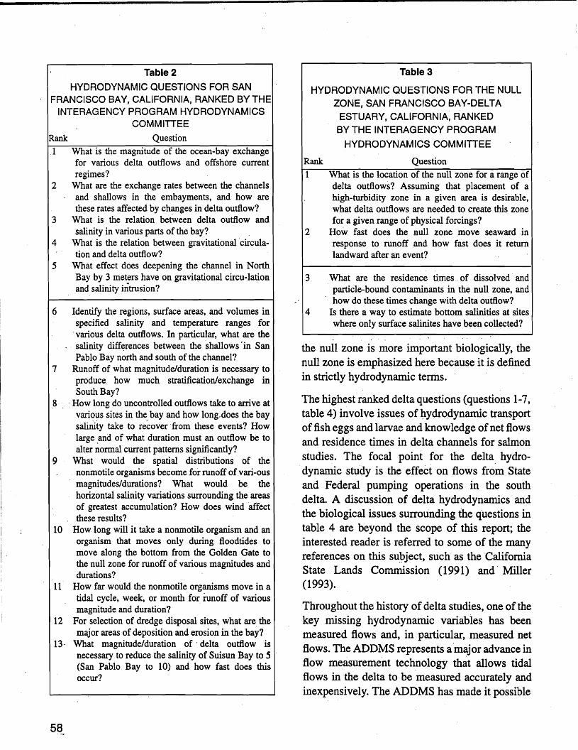
Table 2

HYDRODYNAMIC QUESTIONS FOR SAN FRANCISCO BAY, CALIFORNIA, RANKED BYTHE

INTERAGENCY PROGRAM HYDRODYNAMICS COMMITIEE

Rank Question ,1 What is the magnitude of the ocean-bay exchange

for various delta outflows and offshore current regimes?

2 What are the exchange rates between the channels and shallows in the embayments, and how are these rates affected by changes in delta outflow?

3 What is the relation between delta outflow and salinity in various parts of the bay?

4 What is the relation between gravitational circula­tion and delta outflow?

5 What effect does deepening the channel in North Bay by 3 meters have on gravitational circu-lation and salinity intrusion?

6 Identify the regions, surface areas, and volumes in specified salinity and temperature ranges for

.various delta outflows. In particular, what are the salinity differences between the shallows'in San Pablo Bay north and south of the channel?

7 Runoff of what magnitude/duration is necessary to produce. how much stratification/exchange in South Bay?

8·· How long do uncontrolled outflows take to arrive at various sites in the bay and how long.does the bay salinity take to recover 'from these events? How large and of what duration must an outflow be to alter ~ormal current patterns significantly?

·9 What would, the spatial distributions of the nonmotile organisms become for runoff of vari-ous magnitudes/durations? What would be the horizontal salinity variations surrounding the areas of greatest accumulation'? How does wind affect these results?

10 How long will it take a nonmotile organism and an organism that moves only during floodtides to move along the bottom from the Golden Gate to the null zone for runoff of various magnitudes and durations?

11 How far would the nonmotile organisms move in a tidal cycle, week, or month'for runoff of various

. magnitude and duration? 12 For selection of dredge disposal sites, what are the

major areas of deposition and erosion in the bay? 13· What magnitude/duration of' delta outflow is

necessary to reduce the salinity of Suisun Bay to 5 (San Pablo, Bay to 10) and how fast does this occur?

Table 3

HYDRODYNAMIC QUESTIONS FOR THE NULL ZONE, SAN FRANCISCO BAY-DELTA

ESTUARY, CALIFORNIA, RANKED BY THE INTERAGENCY PROGRAM

HYDRODYNAMICS COMMITIEE

Rank Question

1 What is the location of the null zone for a range of delta outflows? Assuming that placement of a high-turbidity zone in a given area is desirable, what delta outflows are needed to create this zone for a given range of physical forcings?

2 How fast does the null zone move seaward in response to runoff .and how fast does it return landward after an event?

3 What are the residence times. of dissolved and particle-bound contaminants in the null zone, and how do these times change with delta outflow?

4 Is there a way to estimate bottom salinities at sites where only surface salinites have been collected?

the null zone is more important biologically, the null zone is emphasized here because it is defined in strictly hydrodynamic terms.

The highest ranked delta questions (questions 1-7, table 4) involve issues of hydrodynamictransport of fish eggs and larvae and knowledge of net flows and residence times in delta channels for salmon studies. The focal point for the delta, hydro­dynamic study is the effect on flows from State and Federal pumping operations in the south delta. A discussion of delta hydrodynamics and the biological issues surrounding the questions in table 4 are beyond the scope of this report; the interested reader is referred to some of the many references on this subject, such as the 'California State Lands Commission (1991) and' Miller (1993).

Throughout the history of delta studies, one of the key missing hydrodynamic variables has been measured flows and, in particular, measured net flows. The ADDMS represents a major advance in flow measurement technology that allows tidal flows in the delta to be measured accurately and inexpensively. The ADDMS has made it possible.

58

Table 4 HYDRODYNAMIC QUESTIONS,FOR THE SACRAMENTO-SAN JOAQUIN DELTA,

CALIFORNIA, RANKED BY THE INTERAGENCY PROGRAM HYDRODYNAMICS COMMITIEE

Rank Question 1 For salmon studies, the greatest need is for

knowledge of flow magnitudes and directions and residence times in delta channels.

2 For striped bass studies, the most important question is how much delta outflow is required to move larval fish from the delta to Suisun Bay and keep them there.

3 Where are striped bass eggs and larvae transported within the delta? How can project operations be changed to transport them to areas of high food abundance, recognizing that such areas may no longer be in the zone of high turbidity?

4 If zooplankton stocks remain low in Suisun Bay because of Potamocorbula and other benthic bivalves, how can entrainment losses of larvae that remain in the delta be minimized?

5' .If striped bass eggs are transported through the delta in pulses, how might the flow be manipulated for short periods to move pulses into Suisun Bay?

6 Does export pumping affect the flow at the cross-channel gates?

7 Have operational variations of Clifton Court Forebay affected larval entrainment?

8 What is the degree of exposure of striped bass eggs and larvae to rice pesticides that enter the Sacramento River with irrigation water?

9 What is the real variation of delta outflow over a spring-neap cycle, and how is it affected by atmospheric pressure?

10 During export pumping, what is the salinity difference in the western delta between open and closed cross-channel gates?

11 What are the relative contributions of flood control, channelization, and water project storage and diversions on delta outflow?

12 A way of predicting the routes and travel times through the delta of water from different sources is needed for development of sampling schemes of dissolved and particle-bound pesticides and for analyses of pesticides data.

13 Is there a way to estimate bottom salinities at sites where only surface salinities have been collected?

14 Given that dredge materials are used to reinforce delta levees, which levees have the potential for releasing toxic materials to parcels of water that reach municipal or industrial water intakes?

to operate and calibrate continuous monitoring stations for flows in the delta using ultrasonic velocity meters (UVMs). Tidal flows measured by UVMs can be averaged over each tidal cycle to obtain the time variation in net flows. Installing UVM measuring stations at key locations in the delta is one of the main elements of the delta hydrodynamic study.

Details of the hydrodynamic workplan were completed in 1991t and the studies were begun in 1992. In 1994, the time schedule for completing workplan tasks was extended to the end of calendar year 1995. The workplans and studies are discussed in the following two sections begin­ning with the San Francisco,Bay (including null zone) studies, followed by the delta studies. Currently (1995), the new study is nearly

" completed. The emphasis in this chapter is on presenting the workplan rather than on summarizing progress on the work tasks. Results on the new study are due to be reported in 1996.

Bay Studies

The me decided that to answer the San Francisco Bay and null zone questions, a continuing study using multidimensional numerical .modeling, combined with collection and analysis of field data, would offer the best chance for success. The considerable investment of time and resources already spent programming and refining numer­ical models and purchasing and testing the latest field instruments in the earlier program would benefit the study team in the new program. The present (1995) San Francisco Bay study has three main parts. The first part is to conduct a field experiment and 2-D (vertically averaged) mod­eling of Suisun Bay to provide a physical descrip­tion of the null zone region and the processes controlling the salt balance. The second part is to continue operating the network of monitoring stations for water level and salinity in the bay and to analyze the data using powerful time-series and statistical techniques leading toward an improved understanding of the processes that affect salt transport in the estuary. The third part is to develop an efficient 3-D hydrodynamic model that

59

is especially suited for the shallow-water environ­ment of San Francisco Bay and that can be used for making long-term (at least seasonal) simu­lations of the bay. As the 3-D model becomes available, it will eventually replace 2-D models and also will be used to answer questions 'on grav­itational circulation and the null zone that involve the vertical dimension of the estuary. The three parts (tasks) of the study are discussed next. A ' fourth task, not discussed, is the continued devel­opment and maintenance of the hydrodynamic data base.

Task 1: Suisun Bay Salt Balance and Null Zone Study

A field and modeling study of Suisun Bay was undertaken .beginning in the winter season of 1992-93. The objectives of the study are:

• To quantify the dominant mixing processes that .I11aintainthe salt balance in Suisun Bay and to establish the relative .importarice of horizontal versus vertical processes;

• To estimate the movement and location of the . null zone during the study period using field

measurements of current profiles obtained with ADCPs; and

• To analyze the mechanisms that tend to stratify and destratify the water column in Suisun Bay during periods of steady and unsteady river , flow. '

Because of the different length scales that char­acterize the vertical and horizontal dimensions in Suisun Bay, the examination of circulation and mixing can be separated into horizontal (vertically uniform) and vertical (depth-dependent) com­ponents. The first category includes tidally driven residual flows, river inflows, .depth-integrated wind-driven flows, and the mixing process of tidal trapping; these processes must be studied at length scales of 50 m or more. The second category includes gravitational circulation, vertical varia­tions in wind-driven flows, and the processes involved in vertical mixing of mass and momen­tum; these processes must be examined at length scales of 1 m or less. The strategy for the study is

60:~

to use a 2-D, vertically averaged, numerical model to study horizontal processes and to use field measurements in the channel to study vertical ' processes. A working hypothesis for the study is that the salt balance in Suisun Bay is maintained largely by the horizontal processes, except during transient periods of strong gravitational circu­lation associated with runoff. The assumption also is made that, although the physical concept of a null zone is based on the gravitational circulation, the horizontal mixing processes control much of the movement of particles that become entrapped seaward of the null zone and create an entrapment zone of high turbidity. '

Experimental studies

Two experimental field studies are part of the ori­" ginal workplan. The first study was -done during

the winter of 1992-93 from December to April. The second was done during .the .late spring of! 1994. A third field study was carried 'out in late spring and summer of 1995 that was not part of the original workplan; it was added in 1994. This third study is not discussed here.

Winter 1992-93 experiment-The instruments used during this experiment were· deployed as illustrated in figure 28. The most important data were collected from the three ADCPs deployed along the longitudinal axis of the main channel in Suisun Bay at" the three locations' shown (near Chipps Island, Middle Point, and Point Edith).­Time series of tidal velocity profiles were meas-, ured by each instrument at lO-minute intervals. and saved for later analyses. Salinity sensors were deployed at the top and bottom of the water column near the Middle Point and the Point Edith ADCPs and at one additional main channelloca­tion near Roe Island. Single salinity sensors also' were deployed in the shallow waters of Grizzly; and Honker Bays. Salinity measurements at two depths' were .available from the Mallard Island, monitoring station (fig. 6), which is adjacent to the; Chipps Island ADCP. The salinity sensors " recorded time series of salinity that will be used to • determine vertical variations in salinity stratifi-, cation and to estimate salt fluxes. The Chipps Island and Point Edith ADCPs are narrow band

I

122°10' 122°00'

• .. ::~. -... ~ ..... :;'.:.':'~:"'..~ ..:'.:~.:-:.;.•~-4:.:: •.• ~~:.l~~:~~

. I EXPLANATION I ....<,­ •• ,:~' ••:~~: •.... _....,..

38°10' 1-1 ~ Conventional current meter

f'~:~ -;~~~:.~.-; .:;: J ..~ ,:,' •• Salinity sensor

~L~1:;~~i:·/~~:~.~~·::'~ ..~_, .... "":~:• Conventional current meterand salinity sensor

-2- Balhymelrycoolour inteJVal is. • ~ __~

el '~"I ",~...,...."",. "" '!:,••2meers. t ',..-......... : .::.;., ."..' ,.'';; :'••a.' • ••• . \:it . ..: ••Control volume ~~~;.. ~:: .,~~;:;

D = Doppler nb = narrow-baad ,bb =broad-ban

Sd = DataSonde Salinity sensor

S = Ocean sensors Salinity o and Pressure

V =Endeco Current Metere

' .~ .....

"" .

121°50'

38°05'

~

1 ·::-: ;

.Y:.~"

.:.~.eo:,·' ... r-0-:· .:~.

':':::~~:':;~(:~rt:~~+

38°00' ......:: .... :.':~:.I:.:.,:. : .• : .:.:: .:...::::-r.;: .•~.•'..: •.:.:v.': ::0:.. '. . ... ..

Figure 28

LOCATIONS OF INSTRUMENTS DEPLOYED IN SUISUN BAY, CALIFORNIA, DURING THE WINTER 0> EXPERIMENT OF 1992-93. . ,;"",a,.

~j

i.toA.._

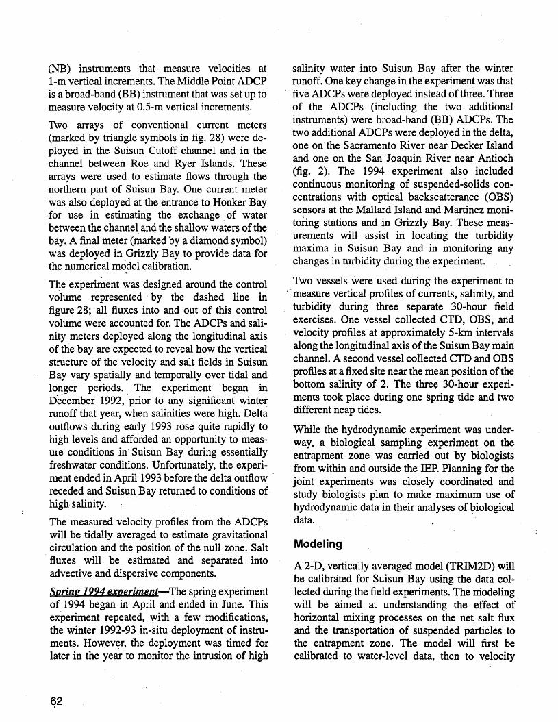
(NB) instruments that measure velocities at l-m vertical increments. The Middle Point ADCP is a broad-band (BB) instrument that was set up to measure velocity at O.5-m vertical increments.

Two arrays of conventional current meters (marked by triangle symbols in fig. 28) were de­ployed in the Suisun Cutoff channel and in the channel between Roe and Ryer Islands. These arrays were used to estimate flows through the northern part of Suisun Bay. One current meter was also deployed at the entrance to Honker Bay for use in estimating the exchange of water between the channel and the shallow waters of the bay. A final meter (marked by a diamond symbol) was deployed in Grizzly Bay to provide data for the numerical model calibration.

The experiment was designed.around the control volume represented' by the dashed line in figure 28; all fluxes into and out of this control volume were accounted for. The ADCPs and sali­nity meters deployed along the longitudinal axis of the bay are expected to reveal how the vertical structure of the velocity and salt fields in Suisun Bay vary spatially and temporally over tidal and longer periods. The experiment began' in December 1992, prior to any significant winter runoff that year, when salinities were high. Delta outflows during early 1993 rose quite rapidly to high levels and afforded an opportunity to meas­ure conditions in Suisun Bay during essentially freshwater conditions. Unfortunately, the experi­ment ended in April 1993 before 'the delta outflow' receded and Suisun Bay returned to conditions of high salinity.

The measured velocity profiles from the ADeps will be tidally averaged to estimate gravitational circulation and the position of the null zone. Salt

. fluxes will be estimated and separated into advective and dispersive components.

Sprine 1994 experiment-The spring experiment of 1994 began in April and ended in June. This experiment repeated, with a few modifications, the winter 1992-93 in-situ deployment of instru­ments.However, the deployment was timed for later in the year to monitor the intrusion of high

salinity water into Suisun Bay after the winter runoff. One key change in the experiment was that five ADCPs were deployed instead of three. Three of the ADCPs (including the two additional instruments) were broad-band (Bfs) ADCPs. The two additional ADeps were deployed in the delta, one onthe Sacramento River near Decker Island and one on the San Joaquin River near Antioch (fig. 2). The 1994 experiment also included continuous monitoring of suspended-solids con­centrations with optical backscatterance (OBS) sensors at the Mallard Island and Martinez moni­toring stations and in Grizzly Bay. These meas­urements will assist in locating the turbidity maxima in Suisun Bay and in monitoring any changes in turbidity during the experiment.

Two vessels were used during the experiment to -: measure vertical profiles of currents, salinity, and

turbidity during three separate 30-hour field exercises. One vessel collected CTD, OBS, and velocity profiles at approximately 5-km intervals along the longitudinal axis of the Suisun Bay main channel. A second vessel collected eTD and OBS profiles at a fixed site near the mean position of the bottom salinity of 2. The three 3D-hour experi­ments took place during one spring tide and two different neap tides.

While the hydrodynamic experiment was under­way, a biological sampling experiment on the entrapment zone was carried out by biologists from within and outside the IEP. Planning for the joint experiments was closely coordinated and study biologists plan to make maximum use of hydrodynamic data in their analyses of biological data.

Modeling

A 2-D, vertically averaged model (TRIM2D) will be calibrated for Suisun Bay using the data col­lected during the field experiments. The modeling will be aimed at understanding the effect of horizontal mixing processes on the net salt flux and the transportation of suspended particles to the entrapment zone. The model will first be calibrated to water-level data, then to velocity

data, and finally to salinity data. A detailed cali­bration' of a 2-D model using measured salinities in San Francisco Bay has not been attempted and could prove to be time consuming. Simulations of salt concentrations require accurate detennina­tions of residual currents and are sensitive to the model coefficients used to parameterize both bottom friction and horizontal mixing. The study will include testing and evaluating several different submodels for the horizontal diffusion process.

A 3-D model presently(1995) is not available for field application to study the transport of salt. The development of a model for that purpose is the task of the hydrodynamic study that is proceeding simultaneously with this study. If it becomes apparent that 3-r5 calculations are in~eed needed for Suisun Bay, then 3-D modeling' will be inte­grated into the study as the model becomes ,available,

Task 2: Operate Monitoring St~tions and Analyze Data

Thernonitoring stations for water temperature, salinity, water level, and meteorology "(see fig. 6) have continued to operate during the new pro­gram, with the exception of moving the Fort Point salinity station to the, south pier of the Golden Gate Bridge in November 1994. The site will be moved again in 1996 or 1997 when seismic retrofit work is scheduled for the bridge.

Analyses of the water-level and s.~inity­

monitoring data are continuing and have been expanded to include the statistical technique of principal components analysis. The data analyses aid in the understanding of the underlying causes for variability in tidally averaged water level and salinity in San Francisco Bay, and, in' particular, how much variability is related to delta outflow, With the recent (December 1994) agreement by state'and federal agencies to impose a bottomsali-_ nity standard of 2 for Suisun Bay, these analyses will attempt to explore how much the location of a bottom salinity of 2 is controlled by delta out­flow and how much is controlled by factors that are not regulated, such as tides and meteorological events.

Task 3: Three-Dimensional Modeling

The third task under the new program is to de­velop a3-D, hydrodynamic model specially suited for making efficient simulations of San Francisco Bay. Before describing the new model, a dis~

cussion of the models mentioned in Chapter 3 and why they will not be used in the new program follows.

Estuarine hydrodynamic software model, three-dimensional

The most serious drawback of the EHSM3D is , that it executes too slowly on workstations to be used successfully for large scale, seasonal appli­cations to San Francisco Bay. For example, on a 50-megahertz workstation, the model requires nearly real time to, run simulations of the entire

'-bay using a coarse grid size of O.5km square. Although run times approximately 10 times faster can be achieved on a supercomputer, the cost is p~ohibitive.· .

EHSM3D is not formulated with a strongly stable numerical algorithm. For the application to San Pablo Bay, the model input' bathymetry and solu­tion variables were smoothedconsiderably before. a stable solution was obtained. The smoothing could have made the model predictions overly diffused.

Although,' theoretically, EHSM3D could be re­coded for greater efficiency and improved stabi­lity, in practice, recoding would not be any easier than developing a new model. Because the docu­mentation available for EHSM3D is limited, interpretation and modification of the computer code would be difficult. In addition, the most efficient algorithms for 3-D modeling of San Francisco Bay are different in structure from those u~ed in EHSM3D and would not easily fit into the framework of the EHSM3D modeling system.

Estuarine, coastal, and ocean model-,'semi-implicit

Although. the computer run time of ECOM-si is significantly faster than EHSM3D, it. is still not optimum for efficient applications to San Francisco Bay. ECOM-si 'incorporates a

63

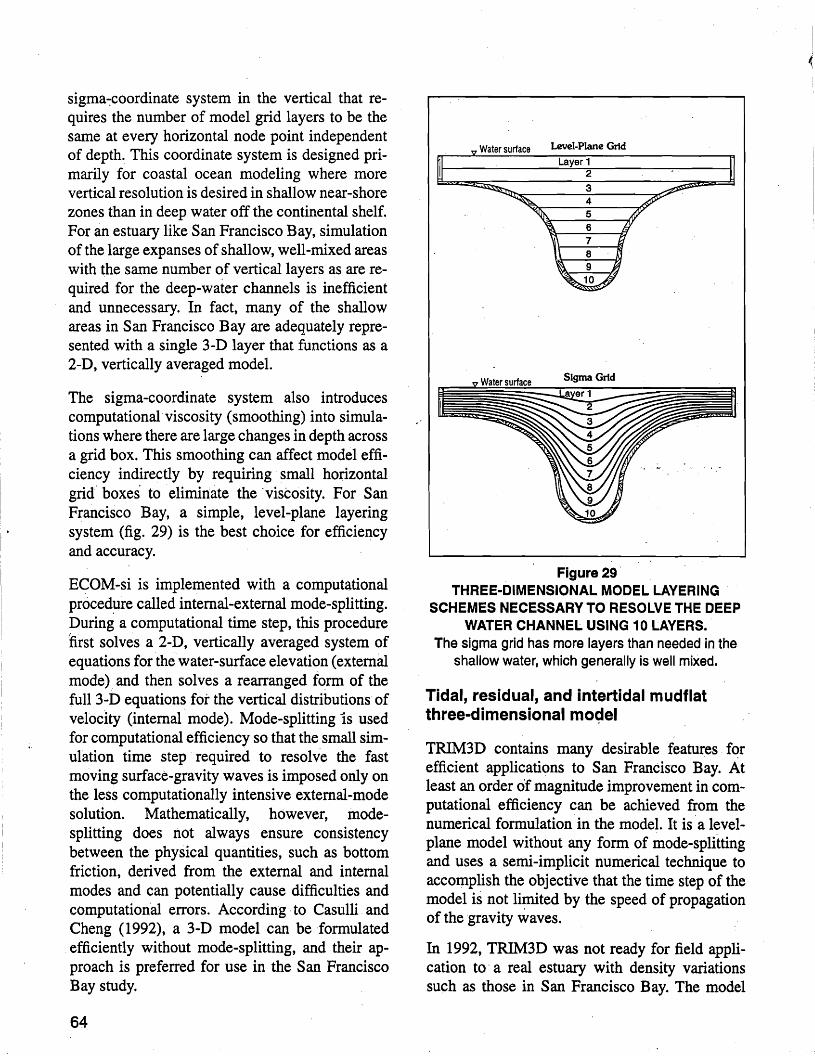
sigma-coordinate system in the vertical that re­quires the number of model grid layers to be the same at every horizontal node point independent of depth. This coordinate system is designed pri­marily for coastal ocean modeling where more vertical resolution is desired in shallow near-shore zones than in deep water off the continental shelf. For an estuary like San Francisco Bay, simulation of the large expanses of shallow, well-mixed areas with the same number of vertical layers as are re­quired for the deep-water channels is inefficient and unnecessary. In fact, many of the shallow areas in San Francisco Bay are adequately repre­sented with a single 3-D layer that functions as a 2-D, vertically averaged model.

The sigma-coordinate system also introduces computationalviscosity (smoothing) into simula­tions where there are large changes in depth across a grid box. This smoothing can affect model effi­ciency indirectly by requiring small horizontal grid boxes' to eliminate the 'viscosity. For San Francisco Bay, a simple, level-plane layering system (fig. 29) is the best choice for efficiency I' and accuracy.

ECOM-si is implemented with a computational procedure called internal-external mode-splitting. During a computational time step, this procedure first solves a 2-D, vertically averaged system of equations for the water-surface elevation (external mode) .and then solves a rearranged form of the full 3-D equations for the vertical distributions of velocity (internal mode). Mode-splitting 1s used for computational efficiency so that the small sim­ulation time step -required to resolve the fast moving surface-gravity waves is imposed only on the less computationally intensive external-mode solution. Mathematically, however, mode­splitting does not always ensure consistency between the physical quantities, such as bottom friction, derived from the external and internal modes and can potentially cause difficulties and computational errors. According to Casulli and Cheng (1992), a 3-D model can be formulated efficiently without mode-splitting, and their ap­proach is preferred for use in the San Francisco Bay study.

64

Figure 29 THREE-DIMENSIONAL MODEL LAYERING .

SCHEMES NECESSARY TO RESOLVE THE DEEP WATER CHANNEL USING 10 LAYERS.

The sigmagrid has more layersthan needed in the shallow water, which generally is well mixed.

Tidal, residual, and intertidal mudflat three-dimensional model

TRIM3D contains many desirable features for efficient applications to San Francisco Bay. At least an order of magnitude improvement in com­putational efficiency can be achieved from the numerical formulation in the model. It is a level­plane model without any form of mode-splitting and uses a semi-implicit numerical technique to accomplish the objective that the time step of the model is not limited by the speed of propagation of the 'gravity waves.

In ·1992, TRIM3D was not ready for field appli­cation to a real estuary with density variations such as those in San Francisco Bay. The model

~.

was not considered for future use in the hydro­dynamic study because the time schedule for its completion could not be estimated. Many of the best features of TRIM3D,' however; .are being included in the 3-D model under development. The in-house code will enable future model studies to be completed considerably quicker than with TRIM3D (or another outside code) because the staff will be familiar with the model pro­gramming, and the familiarity will allow coding changes to be implemented with much less effort.

Development of a new three-dimensional model

In designing the new 3-D model, the following numerical criteria were considered to be important.

• Efficiency, • Second-order accuracy of the numerical solu­

tion algorithm," .

• Mass and momentum conservation,

• No mode-splitting, and

• Oscillation-free advection scheme.

The first and fourth of these criteria are being met by adopting a semi-implicit, finite-difference sol­ution strategy and a level-plane, vertical coor­dinate system as discussed above for TRIM3D. To achieve second-order accuracy in the finite­difference approximations, a three-time-level, leapfrog-trapezoidal scheme is being imple­mented for the time integration technique. Con­servation of mass and momentum are being maintained by.solving the governing equations in a conservative, layer-averaged form and using flux variables as the unknowns. To eliminate any oscillations emanating from the nonlinear advec­tion terms in the model, a special high resolution, flux-corrected transport technique is being used on these terms. A more complete description of the model numerics is presented in a report by Smith and Larock (1993).

The new code is presently (1995) being tested on several problems where known 3-D solutions exist, such as seiching and wind driven flow in a closed rectangular basin. Verification that the

model operatescorrectly on these relatively sim­ple problems before attempting applications to the real estuary is important. Beginning in 1996, the model will be generalized to handle variable geo­metry and arbitrary boundary conditions so that applications to San Francisco Bay can begin. Whether the first application of the model will be made to the entire bay or simply a part of North Bay is undecided. This decision will be made based on the need for modeling studies when the model is ready for field applications. A report on the model detailing the theory, numerics, and testing is due in early 1996.

Delta Studies

Before 1992, the only significant IEP .hydro­dynamic activities. in the delta were the continuous operationIfrom 1987) of two UVMs on Old and Middle Rivers (fig. 30) and the devel­opment and testing (from 1985-87) of a I-D, branching network model by the USBR (Wong and Cheng, 1989). The IEP did not promote delta hydrodynamic studies because, for many years, the DWR has supported its own team of modelers

.who carried out hydrodynamic investigations of the delta..The DWR study team has never been attached administratively to the DWR's IEP staff, but does .collaborate closely with the program members and have completed a number of modeling studies for the IEP. Because the DWR study team concentrates most of its activities in the delta, it originally was intended that the IEP study team would concentrate its activities on hydrodynamic studies needed in the bay part of the estuary. Therefore, the IEP hydrodynamic study team was assigned originally to the Delta­Outflow/San Francisco Bay Study.

By expanding the scope of the new IEP hydrody­namic study to include the delta, the intention is to develop a capability within IEP to carry out delta modeling studies. The IEP can then call upon the

65

12Z00' 45' 121"15'

38°15'

38°00'

381)0'

. 37"45'

. ....

EXPLANATION

• UVM STATION

8, I

12 KiLOMETERS

4

" I 'i 8

. , I 4

NORTHBAY AQU£DUCT~ - ' ~ ~

/~ ,, (

,...._,...;o.~ ..-'" ~.

o I o

Pittsburg 0

---..~~ °Antioch ) ,~utch

' :'. " .' ~" " ~""-~ I---'FmlIIIII.

Figure 30 LOCATIONS OF EXISTING AND PLANNED CONTINUOUS FLOW

MEASURING STATIONS WITH ULTRASONIC VELOCITY METERS IN THE SACRAMENTO-SAN JOAQUIN DELTA, CALIFORNIA.

66

USGS study team or the DWR study team for modeling support. The delta program involves a close collaboration between the USGS and the DWR study teams. The plans are to develop a public domain flow and transport model of the delta and to collect flow data for the calibration and verification of the model. When the model is completed, it will be available to all interested parties and will be used to answer the questions listed in table 4. The two tasks in the delta studies program-(I) model development and (2) flow data collection-are discussed below. Develop­ment of the model is being done by the DWR, and the flow data collection is being done by the USGS. The two agencies meet regularly to agree on the major decisions in the study.

Task 1: Model Development

The delta flow and transport model that presently (1995) is being used by the DWRis referred to as . DWRDSM (DWR .delta ~im:ulation model). Although DWRDSM is the product of the pro­gramming staff at the DWR, it does contain some program modules that are adopted from an earlier proprietary model called the Fischer delta model (FDM) (Fischer, 1982). Because of these proprie­tary modules, the DWRDSM code cannot be dis­tributed freely to all agencies in the IEP or to other potential users. The plan, therefore, is to replace the proprietary modules in DWRDSM so that the reprogrammed model will be available in the public domain. The primary goal of replacing the delta model, however, is not to obtain a.public domain model, but to develop a model that conserves mass, is efficient, and can accept nonprismatic channel geometry as input.

Most of the proprietary modules in DWRDSM involve the numerical solution algorithm that is used to do the flow and transport routing. The algorithm is based on the fixed-grid method of characteristics (MOC) (Lai, 1967; Lai and Onions, 1976). Although the MOC has a number of appealing features, it also has several short­comings that have, in general, led investigators to prefer implicit, finite-difference .methods. One serious shortcoming of the MOC is that it does not guarantee that water and salt mass are conserved

during a simulation. The DWR has determined that, with DWRDSM, the loss of mass during a 1­year simulation of the delta can be significant (Francis Chung, California Department of Water Resources, oral commun., 1993). The overall effect of the loss of mass on the accuracy of predictions is not known, but is worrisome. The MOC also is subject to a restrictive limitation on the maximum size of the simulation time step needed to guarantee the stability of a calculation. For the numerical grid being used with DWRDSM, the time step must be kept to less than or equal to 1 minute, which is much smaller than is needed for accuracy considerations. The time steps of implicit, finite-difference methods are not . limited by stability, so these methods can be used with much larger time steps. Accurate hydro­

" dynamic predictions for the delta using a 15- . minute time step was obtained using an implicit, finite-difference model (Richard Oltmann, USGS, oral .commun., 1993). Obviously, the size of the time step will greatly affect the run time of simu­lations. Also, the MOC algorithm in DWRDSM is not formulated to accept arbitrarily shaped chan­nel geometry data as input; all channel geometry must be idealized into an equivalent rectangular form. Use of the natural channel shapes that represent the real field conditions is desirable.

Several alternative flow routing algorithms have been evaluated by the DWR to replace the MOC

, in DWRDSM. A decision was made to adopt the standard four-point Priessman implicit, finite­difference scheme (Priessman, 1961) as imple­mented in the USGS FoURPT model (DeLong, 1993). The four-point scheme is well proven in other operational unsteady-flow models, such as the National Weather Service model (Fread, 1985), and has become somewhat of a standard method against which others are compared. Testing of the FoURPT model by the DWR on several simple networks has demonstrated that it conserves mass exactly. The model is at least as efficient as the MOC and can run larger time steps without becoming unstable or sacrificing accur­

. acy. The code is well documented with comment statements, which will be helpful when program modifications and additions need to be made.

67

, ­

The salt-transport model in DWRDSM is being replaced with a Lagrangian routing model called BLTM (hranched Lagrangian transport model) (Jobson and Schoellhamer, 1987). Lagrangian means the model operates with a moving coor­dinate system that follows individual water parcels while continuously tracking the salt con­centration of each parcel. This approach conserves salt mass exactly and provides an accu­rate solution to the salt-transport equation. In the new delta .model, the BLTMmodule will be numerically coupled to the FoURPT hydro­dynamic module so that the model will include forcing of the flow by horizontal density gradi­ents. Previous models of the delta have neglected density-gradientforcing, which is important in the west delta. .

Both the FouRPT and BLTM modules are de­signed to accept natural channel geometry, so a new set of channel geometry input for the model will be developed from available data. Some collection of new 'geometry data is planned. The DWR team is in the process of developing a delta channel-geometry data base to facilitate the handling and updating of model geometry data.

Task 2: Flow Data Collection

To improve the accuracy of predictions with the new delta model, additional flow data are needed forcalibrating and verifying the model. Obtaining conventional discharge measurements in the delta is difficult and expensive; therefore, relatively few measurements have been made. These meas­urements and available water-level data were used in the calibration of the DWRDSM. Because transport processes in the delta largely are controlled by tidally averaged (residual) flows, there is a strong need for continuous flow meas­urements that can be averaged over tidal cycles and longer periods for comparison with model simulations.

Flow can be measured continuously in the delta by using DVMs (Laenen, 1985). These instruments (previously called acoustic velocity meters or AVMs) send an acoustic signal across a channel at approximately a 45-degree angle to the primary flow direction. By measuring the time-of-travel of the .signal along its path, an estimate of the path­or line-integrated velocity is obtained. The line velocity is converted to total flow by multiplying it by a coefficient and the channel cross-sectional area. The coefficient must be determined by calibration with measured discharges.

Although DVMs have been available for some time, the inability to make the necessary discharge measurements needed to calibrate the DVM limited the use of the technology in the delta. The

-- availability of the ADDMS to make fast, accurate, and economical discharge measurements makes DVM discharge. measuringstations. practical in the delta.' . . .

As part of the new plan, in addition to the two existing UVM stations on Old and Middle Rivers, six new UVM discharge measuring stations are being installed in the delta and calibrated with the ADDMS. The locations of the stations were chosen to provide data on certain critical flow splits among the delta channels and good geo­graphical coverage for use in flow model cali­bration and verification. The locations of the'eight stations are shown in figure 30. . .

As the DVM data become available, they will be used with other flow and water-level data to calibrate and verify the new delta model. If the calibration process reveals a need for additional tidal discharge measurements, the ADDMS will be used to collect the data. The USGS will collab­orate with the DWR in the calibration/verification process for the model.

68

[_.. -

LITERATURE CITED

Armor, C. and P.L. Herrgesell. 1985. Distribution and abundance of fishes in the San Francisco Bay estuary between 1980 and 1982. In: Temporal Dynamics ofan Estuary-San Francisco Bay. J.E. Cloern, and F.H. Nichols, eds. Hydrobiologia. 129:211-227.

Arthur, J.F., and M.D. Ball. 1979. Factors influencing the entrapment of suspended materials in San Francisco Bay­Delta estuary. In: San Francisco Bay-The Urbanized Estuary, TJ. Conomos. ed., Pacific Division, Amer. Asso. Advance. Sci. San Francisco, CA. pp. 143-174.

__. 1980. The Significance of the Entrapment Zone Location to the Phytoplankton Standing Crop in the San Francisco Bay-Delta Estuary. U.S. Bureau of Reclamation Technical Report. Sacramento, CA. 89 pp!

Brumley, B.H., R.G. Cabrera, K.L. Deines, and E.A. Terray. 1991. Performance of a broad-band acoustic Doppler current profiler. 1. Oceanic Engineering. 16(4):402-407.

Burau, J.R., and R.T. Cheng. 1988. Predicting tidal currents in San Francisco Bay using a spectral model. In: Proceedings ofthe 1988 National Conference on Hydraulic Engineering, Amer. Soc. Civil Eng. Colorado

. Springs, ~O. August 8-12, 1988. pp. 634-639. ­

.,__. 1989a, A Vertically Averaged Spectral Model for Tidal Circulation in .Estuaries-Part 1. Model Formulation. U.S. Geological Survey. Water-Resources Investigations Report 88-4126.31 pp.

__. 1989b. A General Method for Generating Bathymetric Data for Hydrodynamic Computer Models. U.S. . 'Geological Survey Open-File Report 8?-28. 45 pp.

. ~" t . Burau, J.R., M.R. Simpson, and R.T. Cheng. 1993. Tidal and Residual Currents Measured by an Acoustic Doppler

Current Profilerat the West End ofCarquinez Strait, San Francisco Bay, California, Marchto November 1988. U.S. Geological Survey Water-Resources Investigations Report 92-4064.79 pp.

California Department of Fish and Game: 1989. Striped Bass Restoration and Management Plan for the Sacramento-San Joaquin Estuary. Phase I. 39 pp.

California Department of Water Resources, ·1986. DAYFLOW Program Documentation and DAYFLOW Data Summary User's Guide.

__. 1995. DAYFLOW Data Summaryfor Water Year 1994.

California State Lands Commission. 1991. Delta-Estuary, California's Inland' Coast. A Public Trust Report. May 1991. 208 pp. .

Casulli, V., and R.T. Cheng. 1992. Semi-implicit fmite difference methods for three-dimensional shallow water flow. Int. 1. for Numerical Methods in Fluids. 15:629-648.

Cayan, D.R., and D.H. Peterson. 1993. Spring climate and salinity in the San Francisco Bay Estuary. Water Resour. Res. 29(3):293-303.

Cheng, R.T., and V. Casulli. 1982. On Lagrangian residual currents with applications in South San Francisco Bay, California. Water Resour. Res. 18(6):1652-1662.

Cheng, R.T., V. Casulli, and J.W. Gartner. 1993. Tidal, residual, intertidal mudflat (TRIM) model and its applications to San Francisco Bay, California. Estuarine Coastal and ShelfScience. 36:235-280.

Cheng, R.T., and J.W. Gartner. 1984. Tides and Tidal Residual Currents in San Francisco Bay, California-Results ofMeasurements, 1979,-1980. U.S.Geological Survey Water-Resources Investigations Report 84-4339. 319 pp.

__. 1985. Harmonic analysis-of tides and tidal currents in South San Francisco Bay, California. Estuarine Coastal and ShelfScience. 21:57-74.

69

Cloern, J.E. 1984. Temporal dynamics and ecological significance of salinity stratification in an estuary (South San Francisco Bay, USA). Oceanologica Acta. 7(1):137-141.

Cloern, J.E., T.M. Powell, and L.M. Huzzey. 1989. Spatial and temporal variability in South San Francisco Bay. n. Temporal changes in salinity, suspended sediments, and phytoplankton biomass and productivity over tidal time scales. Estuarine Coastal and ShelfScience. 28:599-613.

Conomos, T.J. 1979. Properties and circulation of San Francisco Bay waters. In: San Francisco Bay-The' Urbanized Estuary, T.J. Conomos. ed., Pacific Division, Amer. Asso. Advance. Sci. San Francisco, CA. pp.47-84.

DeLong, L.L. 1993. A numerical model for learning concepts of streamflow simulation. In: Proceedings ofthe 1993 National Conference onHydraulic Engineering. Amer. Soc. Civil Eng. San Francisco, CA. July 25-30, 1993.pp.1586-1591.

Fischer, H.B. 1982. DELFLO and DELSAL, Flow and Transport Models for the Sacramento-San Joaquin Delta. Description and Steady-State Verification. Hugo B. Fischer, Inc. Berkeley, CA. Report HBF 82101.

Fischer, H.B., E.J. List, R.C.Y. Koh, J. Imberger, and N.H. Brooks. 1979. Mixing in Inland and Coastal Waters. Academic Press. New York. 483 pp.

Ford, M., J. Wang: and R.T. Cheng. 1990. Predicting the vertical structure of tidal current and salinity in San Francisco Bay, California. Water Resour. Res. 26{5):1027-1045.

Fox, J.P., T.R. Mongan, and W.J. Miller. 1990. Trends in freshwater inflow to San Francisco Bay from the Sacramento-San Joaquin Delta. Water Resour. Bull. 26(1):101-116.

Fr~~d,D.L. 1985. Channel routing, Chapter 14. In: Hydrological Forecasting, M.G. Anderson and T.P. Burt, eds. John Wiley and Sons, New York. pp. 437-503.

Gartner, J.W., and R.N. Oltmann. 1985. Comparison of recording current meters used for measuring velocities in shallow waters of San Francisco Bay, California. In: Proceedings of the Ocean Engineering and the Environment Conference: Institute of Electrical and Electronics Engineers Ocean Engineering Society. San Diego, CA. pp. 731-737.

__.1990. Comparison ofRecording Current Meters in Shallow Waters ofSan Francisco Bay, California. U.S. Geological Survey Water-Resources Investigations Report 90-4018.84 pp.

Gartner, J.W., and B.T. Yost. 1988. Tides, and Tidal and Residual Currents in Suisun and San Pablo Bays, California-Results of Measurements, 1986. U.S. Geological Survey Water-Resources Investigations Report 88-4027. 94 pp. - ,

Godin, G. 1972. The Analysis ofTides. University of Toronto Press. 264 pp.

Hachmeister, L.E. 1987. Hydrodynamics of the Central and Northern Reaches of the San Francisco Bay-Delta Estuary. U.S. Bureau of Reclamation exhibit No. 109 to State Water Resources Control Board 1987 San Francisco BaylDelta hearings. 20 pp.

Herbold, Bruce, A.D. Jassby, and P.B. Moyle. 1992. Status and Trends Report on Aquatic Resources in the San Francisco Estuary. Report to the U.S. Environmental Protection Agency, San Francisco Estuary Project, San Francisco, CA. 257 pp. plus appendices.

Herrgesell, P.L. comp, 1990.1989 Annual Report. Interagency Ecological Study Program for the S~cramento-San Joaquin Estuary. 112 pp.

Herrgesell, P.L., M.A. Kjelson, J.A. Arthur, L. Wintemitz., and P. Coulston. 1993. A Review of the Interagency Ecological Studies Program and Recommendations for its Revision. Prepared for the agency coordinators of the Interagency Ecological Studies Program, Sacramento, CA. 75 pp.-

Herrgesell, P.L., R.G. Schaffer, and C.T. Larsen. 1983. Effects of Freshwater Outflow on San Francisco Bay Biological Resources. Sacramento, CA. Interagency Ecological Studies Program for the Sacramento-San Joaquin Estuary Technical Report 7.86 pp. .

70

____________________________

Jassby, A.D., W.1. Kimrnerer, S.G. Monismith, C. Armor, J.E. Cloern, T.M. Powell, r.a. Schubel, and T.1. Vendlinski. 1995. Isohaline position as a habitat indicator for estuarine populations. Ecological Applications. 5:1:272-289.

Jobson, H.E., and D.H. Schoellhamer, 1987. Users Manual for a Branched Lagrangian Transport Model. U.S. Geological Survey Water-Resources Investigations Report 87-4163.73 pp.

Kimrnerer, W. 1992. An Evaluation of Existing Data in the Entrapment Zone of the San Francisco Bay Estuary. Sacramento, CA. Interagency Ecological Studies Program for the Sacramento-San Joaquin Estuary Technical Report 33.49 pp.

Krone, R.B. 1972. A Field Study ofFlocculation as a Factor in Estuarial Shoaling Processes. U.S. Army Corps of Engineers Committee on Tidal Hydraulics Technical Bulletin 19, Waterways Experiment Station. Vicksburg, MS. 61 pp. - "

Laenen, Antonius. 1985. Acoustic Velocity Meter Systems. U.S. Geological Survey Techniques of Water-Resources Investigations. Book 3. Chap. A17. 38 pp. '

Lai, Chintu. 1967. Computation of Transient Flows in Rivers and Estuaries by the Multiple-Reach Method of Characteristics. U.S. Geological Survey Professional Paper 575-D. pp. D273-D280.

Lai, Chintu, and C~A. Onions. 1976. Computation of Unsteady Flows in Rivers and Estuaries by the Method of Characteristics. U. S. Geological Survey Computer Contribution. 202 pp. Available only from the U.S. Department of Commerce, National Technical Information Service. Springfield, VA. 22151. Report PB 253785.

Leendertse, J.1., and E.C. Gritton. 1971. A Water-Quality Simulation Modelfor Well-Mixed Estuaries and Coastal Seas. Vol. II. Computation Procedures. Santa Monica, CA. The Rand Corporation. 53 pp.

McCulloch, D.S., D.H. Peterson, P.R. Carlson, and T.J. Conomos. 1970. A Preliminary Study ofthe Effects ofWater Circulation in the San Francisco Bay Estuary: U.S. Geological Survey Circular 637-A. 27 pp.

Miller, W.J. 1993. The Delta, Overview of the Sacramento-San Joaquin Delta. Report prepared for the California Urban Water Agencies. May 1993.49 pp.

Phillips, D.J.H. 1987. Toxic Contaminants in the San Francisco Bay-Delta Estuary and Their Possible Biological Effects. Richmond, CA. San Francisco Bay Aquatic Habitat Institute. 413 pp.

Powell, T.M., J.E. Cloem, and L.M. Huzzey. 1989. Spatial and temporal variability in South San Francisco'Bay, I. Horizontal distributions of salinity, suspended sediments, and phytoplankton biomass and productivity. Estuarine Coastal andMarine Science. 28:583-597.

Preissmann, Alexandre. 1961. Propagation des-intumescences dans les canaux et rivieres [Propagation of translatory waves in channels and rivers]. In: Proc. 1st Congres de l'Assoc. Francoise de Calcul [Proceedings 1st Congress ofthe French Association for Computation.] Grenoble, France. pp. 433-442.

RD Instruments. 1989. Acoustic Doppler Current Profilers-Principles of Operation. A Practical Primer: San Diego, CA. RD Instruments. 36 pp.

Sheng, Y.P. 1983. Mathematical Modeling of Three-Dimensional Coastal Currents and Sediment Dispersion. Model Development and Application. Vicksburg, MS. U.S. Army Corps of Engineers Waterways Experiment Station, Technical Report CERC~83-2. 287 pp. ,

Sheng, Y.P., S.F. Parker, and D.S. Henn. 1986. A Three-Dimensional Estuarine Hydrodynamic Software Model (EHSM3D). Report prepared for the U.S. Geological Survey under Contract no. 14-08-001-21730. 162pp.

Simpson, M.R. 1986. Evaluation of a vessel-mounted acoustic Doppler current profiler for use in rivers and estuaries. In: Proceedings of the Third Working Conference on Current Measurement. Institute of Electrical and Electronics Engineers. Airlie, VA. January 22-24, 1986. pp. 106-121.

71 ~-~-----J

.... o· .;i:..~

Simpson, M.R., and R.N. Oltmann. 1990. An acoustic Doppler discharge-measurement system. In: Proceedings of the 1990 National Conference on Hydraulic Engineering, American Society of Civil Engineers. San Diego, CA. July 30-August 3, 1990. pp. 903-908.

__. 1992. Discharge-Measurement System Using an Acoustic Doppler Current Profiler with Applications to Large Riv,ersand Estuaries. U.S. Geological Survey Water-Suppl~ Paper 2395. 32 pp.

Smith, L.H., and R.T. Cheng. 1987. Tidal and tidally averaged circulation characteristics of Suisun Bay, California: Water Resour. Res. 3(1):143-155.

Smith, P.E. 1994. San Francisco Bay test case for 3-D model verification. In: Proceedings of the 1994 National Conference on Hydraulic Engineering. Amer. Soc. Civil Eng. Buffalo, NY. August 1~5, 1994. pp. 885­889.

Smith, P.E.~R.T. Cheng, J.R. Burau, and M.R. Simpson. 1991. Gravitational circulation in a tidal strait. In: Proceedings of the 1991 National Conference on Hydraulic Engineering. Amer. Soc. Civil Eng. Nashville, TN. July 29-August 2, 1991. pp. 429-434.

Smith, P.E., and B.E. Larock., 1993. A fmite-difference model for 3-D flow in bays and estuaries. In: Proceedings of the 1993 National Conference on Hydraulic Engineering. Amer. Soc. Civil Eng. San Francisco, CA. July 25-30, 1993. pp. 2116-2122. .

Smith, P.E., R.N. Oltmann, and M.R. Simpson. 1992. Data set for verification of 3-D free-surface hydrodynamic models, Carquinez Strait, California. In: Proceedings Hydraulic Engineering Sessions Water Forum '92. Amer. Soc. Civil Eng. Baltimore, MD. August 2-6, 1992. pp. 430-435.

Stelling, G.S., A.K. Wiersma, and J.B.T. Willemse. 1986. Practical aspects of accurate tidal computations. J. Hydraulic Engineering. 112(9):802-817. .

Taylor, MJ., and B.T. Yost. 1989. Description ofSalinity, Temperature, Chlorophyll, Suspended-Sediment, and Velocity Data, South San Francisco Bay, California, February-April 1987. U.S. Geological Survey Open-File Report 89-619. 28 pp.

Thevenot;M.M., and N.C. Kraus. 1993. Comparison of acoustical and optical measurements of suspended material in the Chesapeake Estuary. J. Mar. Environ. Engineering. 1:1:65-79.

Unesco. 1979. Ninth report of the joint panel on oceanographic tables and standards: Unesco Technical papers in Marine Science. 36:24. .

U.S. Environmental Protection Agency. 1992. State of the Estuary-A Report on Conditions and Problems in the San Francisco Bay/Sacramento-San Joaquin Delta Estuary. San Francisco, CA. San Francisco Estuary Project. 270 pp.

Walters, R.A. 1982. Low-frequencyvariationsin sea level and currents in South San Francisco Bay. J. Phys. Ocean. 12:7:658-668.

Walters, R.A., R.T. Cheng, and TJ. Conomos. 1985. Time scales of circulation and mixing processes of San Francisco Bay waters. In: Temporal Dynamics of an Estuary--San Francisco Bay. J.E. Cloern, and F.H. Nichols, eds. Hydrobiologia. 129:13-36.

Walters, R.A., and J.W. Gartner. 1985. Subtidal sea level and current variations in the northern reach of San Francisco Bay. Estuarine, Coastal and ShelfScience. 21:17-32.

Williams, P.B., and L. Fishbain.1987. Analysis of Changes in Delta Outflow Due to Existing and Future Water Development Scenarios. San Francisco, CA. Philip Williams and Associates, Report 412-1. Submitted by the Environment Defense Fund as Exhibit 2, California State Water Resources Control Board, 1987 Water QualitylWater Rights Proceeding on the San Francisco Bay/Sacramento-San Joaquin Delta, California. 11 pp.'

Wong, H.F.N., and R.T. Cheng. 1989. A branched hydrodynamic model of the Sacramento-San Joaquin Delta, California. In: Proceedings ofthe 1989 National Conference on Hydraulic Engineering. Amer. Soc. Civil Eng. New Orleans, LA. August 14-18, 1989. pp. 483-498.