1

Summary Extrapolation Model

Four different flow meters were calibrated under ideal flow conditions at tempera-tures between 10 and 85 °C. The data were used to fit curves for each of them in order to describe the behaviour in a direct or indirect way as a function of tempera-ture. All four flow meters showed a smooth dependency that is easy to extrapolat. For the 10 beam ultrasound flow meter and a magnetic inductive flow meter the dependency to temperature was a direct one, for the orifice plate and the venturi tube the dependency was indirect via Reynolds number. A first fit was extrapolated to indicate the behaviour for temperature and pressure conditions typical for power plants, which means water temperatures between 150 and 300 °C and pressures up to 80 bars. In this report these extrapolation models are now refined to reduce meas-urement uncertainty from extrapolation.

2

Contents

1. Introduction 2. Precondition for the extrapolation work 3. The extrapolation model for the ultrasound meter 4. The extrapolation model for the magnetic induction meter 5. The extrapolation model for the venture tube 6. The extrapolation model for the orifice plate 7. Scaling and general validity of extrapolation References

3

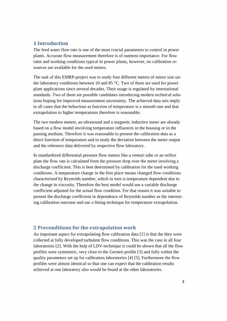
1 Introduction

The feed water flow rate is one of the most crucial parameters to control in power plants. Accurate flow measurement therefore is of outmost importance. For flow rates and working conditions typical in power plants, however, no calibration re-sources are available for the used meters.

The task of this EMRP-project was to study four different meters of minor size un-der laboratory conditions between 10 and 85 °C. Two of them are used for power plant applications since several decades. Their usage is regulated by international standards. Two of them are possible candidates introducing modern technical solu-tions hoping for improved measurement uncertainty. The achieved data sets imply in all cases that the behaviour as function of temperature is a smooth one and that extrapolation to higher temperatures therefore is reasonable.

The two modern meters, an ultrasound and a magnetic inductive meter are already based on a flow model involving temperature influences in the housing or in the passing medium. Therefore it was reasonable to present the calibration data as a direct function of temperature and to study the deviation between the meter output and the reference data delivered by respective flow laboratory.

In standardized differential pressure flow meters like a venturi tube or an orifice plate the flow rate is calculated from the pressure drop over the meter involving a discharge coefficient. This is best determined by calibration for the used working conditions. A temperature change in the first place means changed flow conditions characterized by Reynolds number, which in turn is temperature dependent due to the change in viscosity. Therefore the best model would use a variable discharge coefficient adjusted for the actual flow condition. For that reason it was suitable to present the discharge coefficient in dependence of Reynolds number as the interest-ing calibration outcome and use a fitting technique for temperature extrapolation.

2 Preconditions for the extrapolation work

An important aspect for extrapolating flow calibration data [1] is that the they were collected at fully developed turbulent flow conditions. This was the case in all four laboratories [2]. With the help of LDV-technique it could be shown that all the flow profiles were symmetric, very close to the Gersten profile [3] and fully within the quality parameters set up for calibration laboratories [4] [5]. Furthermore the flow profiles were almost identical so that one can expect that the calibration results achieved at one laboratory also would be found at the other laboratories.

4

3 The extrapolation model for the ultrasound meter

The new 10-beam ultrasound flow meter already has a correction function imple-mented in the flow computer. The meters raw data of the measured flow velocity wRAW is corrected in dependence of pressure p, temperature T and Reynolds number

Re to determine the volume flow rate qv. The refined equation has the following form

qv =km ·kh(Re)·kt(T)·kp(p)·wRAW +Q0 (1)

With kh(Re): 0.9964 Q0: 0.335 m3h-1

The first term, the meter constant km is independent of p, T and Re and is generally

determined by calibration. It also includes geometrical parameters such as the inter-nal cross-section and path angles that cannot easily be determined by other methods with sufficient accuracy. The hydraulic correction term kh was determined in ad-

vance by a factory calibration at 20 C and was later updated based on the available calibration results at PTB. In the refined model the initial hydraulic correction kh was therefore not used in the measurement campaign but the updated correction was applied a posteriori. For the thermal expansion constant kt a linear expansion model

including a linear expansion coefficient was used. The pressure expansion factor kp was not used in this study since a low and constant pressure of 0.2 MPa was pro-vided during all measurements. In addition to these already known parameters [6] it was found necessary to also include an offset term Q0 in the correction, because the

UFM exhibited a clear flow velocity dependency [7].

This behaviour lead to a spread of measured deviations at fixed Reynolds numbers and different temperatures and flow velocities. Q0 was determined by a least squares

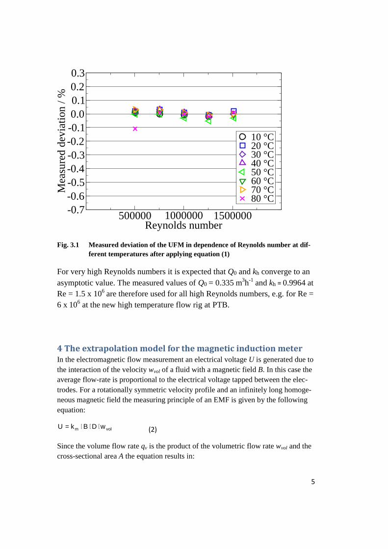
method based on reducing the spread of the measured deviations at the fixed Rey-nolds numbers. The measurements of the UFM include 5 Reynolds numbers and 8 temperatures between 10 C and 80 C. As shown in figure 3.1 the resulting devia-tions after applying all corrections vary about ±0.05 % for all Reynolds numbers. This result implies that the systematic effects are well covered by the presented re-fined correction function given in equation (1).

5

Fig. 3.1 Measured deviation of the UFM in dependence of Reynolds number at dif-ferent temperatures after applying equation (1)

For very high Reynolds numbers it is expected that Q0 and kh converge to an asymptotic value. The measured values of Q0 = 0.335 m3h-1

and kh = 0.9964 at Re = 1.5 x 106 are therefore used for all high Reynolds numbers, e.g. for Re = 6 x 106 at the new high temperature flow rig at PTB.

4 The extrapolation model for the magnetic induction meter

In the electromagnetic flow measurement an electrical voltage U is generated due to the interaction of the velocity wvol of a fluid with a magnetic field B. In this case the average flow-rate is proportional to the electrical voltage tapped between the elec-trodes. For a rotationally symmetric velocity profile and an infinitely long homoge-neous magnetic field the measuring principle of an EMF is given by the following equation:

volm wDBkU ⋅⋅⋅= (2)

Since the volume flow rate qv is the product of the volumetric flow rate wvol and the cross-sectional area A the equation results in:

500000 1000000 1500000Reynolds number

-0.7-0.6-0.5-0.4-0.3-0.2-0.10.00.10.20.3

Mea

sure

d de

viat

ion

/ %

10 °C20 °C30 °C40 °C50 °C60 °C70 °C80 °C

UBk

Dq

mv ⋅

⋅⋅⋅=

4π

(3)

The values of diameter D and plemented in the electronics of the flow meter by the manufacturer. In general also temperature dependencies, e.g. of diameter impossible to have access to the raw data since these are corporate secrets.

Therefore the magnetic inductive meter has been calibrated in terms of the Reynolds numbers corresponding to 5 flow rates and 9 temperatures between 11 and 85 °C. Itcould earlier be shown that the measurement deviation is a linear function of the temperature. This means this meter has more or less no compensation for temperture effects. This is very clearly demonstrated in figure

Fig 4.1 Measurement deviation

for all performed flow rates.

As best refined model for the temperature dependency used for extrapolation to high Reynolds numbers in order to predict a measurement error at temperatures exceeing 200 °C the following equation was ob

Refined model undisturbed flow

with: 0.8 ≤ km ≤ 1.0.

and km · B for the reduced measuring sensitivity are iplemented in the electronics of the flow meter by the manufacturer. In general also

, e.g. of diameter D(T) are mostly implementeimpossible to have access to the raw data since these are corporate secrets.

Therefore the magnetic inductive meter has been calibrated in terms of the Reynolds numbers corresponding to 5 flow rates and 9 temperatures between 11 and 85 °C. It

be shown that the measurement deviation is a linear function of the temperature. This means this meter has more or less no compensation for temperture effects. This is very clearly demonstrated in figure 4.1.

Measurement deviation of the MID in direct dependence of the temperature

for all performed flow rates.

As best refined model for the temperature dependency used for extrapolation to high Reynolds numbers in order to predict a measurement error at temperatures excee

the following equation was obtained:

Refined model undisturbed flow: E[%] = -0.37598 – 3.45812 x 10-9

× Re

6

for the reduced measuring sensitivity are im-plemented in the electronics of the flow meter by the manufacturer. In general also

are mostly implemented. But it is impossible to have access to the raw data since these are corporate secrets.

Therefore the magnetic inductive meter has been calibrated in terms of the Reynolds numbers corresponding to 5 flow rates and 9 temperatures between 11 and 85 °C. It

be shown that the measurement deviation is a linear function of the temperature. This means this meter has more or less no compensation for tempera-

the temperature

As best refined model for the temperature dependency used for extrapolation to high Reynolds numbers in order to predict a measurement error at temperatures exceed-

Re (4)

The effect of the implementing this urement data (undisturbed case) measurement error can be supressedwith an offset of about -0.37 %. The result is almost the same for the disturbed case. The investigated meter innately has a conical reduction of the msection to provide rotationally symmetric velocity profiles nearly independent from the upstream condition.

Fig. 4.2 Measurement deviation of the EMF in dependence of dif ferent temperatures before and after temperature c

5 The extrapolation model for the ventur

The measurement principle for the venturi tube, as for all other differential pressure flow meters, follows from the continuity equation (law of the conservation of mass) and from Bernoulli´s equatirelates the interesting mass flow according to ISO standard

dCq o

m ⋅⋅−⋅

⋅⋅⋅=β

επ2

14 2

2

The effect of the implementing this as temperature correction to the original mea(undisturbed case) is demonstrated in figure 4.2, where the variation in

measurement error can be supressed to lie within a small range of around ±0.05 % 0.37 %. The result is almost the same for the disturbed case.

The investigated meter innately has a conical reduction of the measuring crosssection to provide rotationally symmetric velocity profiles nearly independent from

Measurement deviation of the EMF in dependence of Reynolds number at ferent temperatures before and after temperature correction.

5 The extrapolation model for the venturi tube

The measurement principle for the venturi tube, as for all other differential pressure flow meters, follows from the continuity equation (law of the conservation of mass) and from Bernoulli´s equation. The final measurement equation deduced from these

mass flow qm to the square rot of the pressure difference standard 5167 [8]

dp⋅ρ (5)

7

temperature correction to the original meas-where the variation in

lie within a small range of around ±0.05 % 0.37 %. The result is almost the same for the disturbed case.

easuring cross-section to provide rotationally symmetric velocity profiles nearly independent from

Reynolds number at orrection.

The measurement principle for the venturi tube, as for all other differential pressure flow meters, follows from the continuity equation (law of the conservation of mass)

ent equation deduced from these to the square rot of the pressure difference dp

For an incompressible mediumadditional factor C relatingcase, e.g. frictionless flow rate from Bernoulli’s equationtube the value of this flow rate cclose to a value of 1.0, but it is not a

The calibration of the used classical Venturi tube flow meter with a machined covergent section included 8 temperatures and a number of differeresulting discharge coefficient showed a slight linear dependency with Reynolds number. All measuring results were mainly within the uncertainty limits stated by the standard [11]. In the undisturbed casevalue of one. With a disturber in front in form of an asymmetric swirl generator slightly lower discharge coefficient was measured providing less spread.

In the refined form after having removed data of higher uncertainty tion to the higher Reynolds numbers found the undisturbed and (7) for the disturbed case.

Refined model undisturbed:

Refined model disturbed:

Fig. 5.1 The calibration data of the discharge coefficient for a classical venturi tube at 8 temperatures and several flow rates with and without a disturber ustream fitted with a linear model.

0,994

0,996

0,998

1,000

1,002

1,004

1,006

1,008

1,010

1,012

1,014

0 500000

Me

asu

red

dis

cha

rge

co

eff

icie

nt

CD (undisturbed)

CD (disturbed)

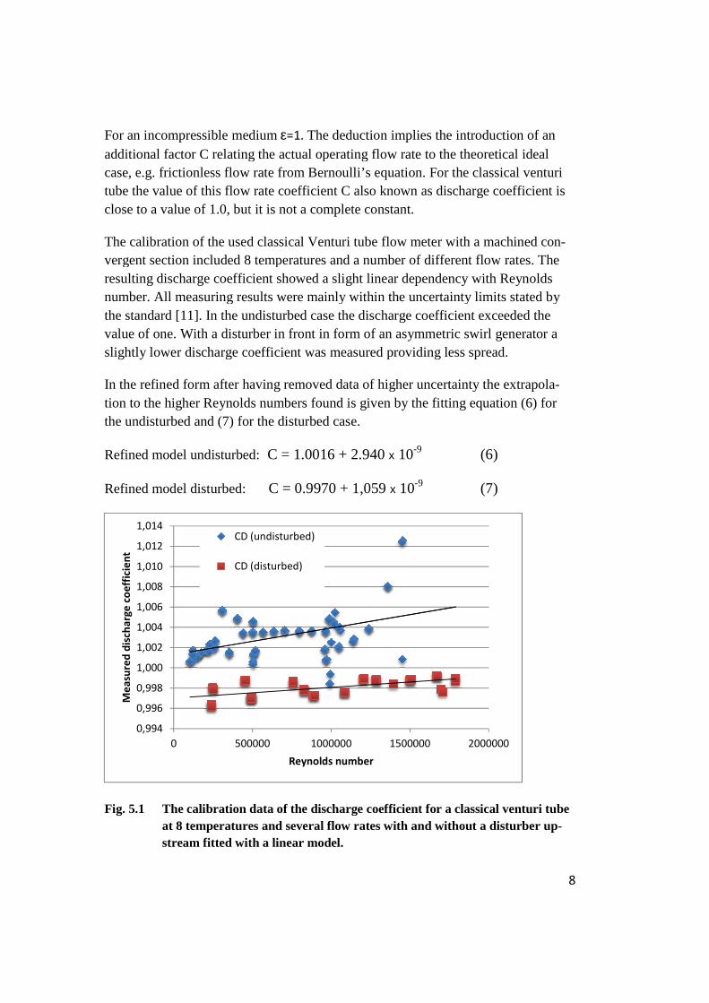
For an incompressible medium ε=1. The deduction implies the introduction of relating the actual operating flow rate to the theoretical ideal

, e.g. frictionless flow rate from Bernoulli’s equation. For the classical venturi tube the value of this flow rate coefficient C also known as discharge coefficiclose to a value of 1.0, but it is not a complete constant.

The calibration of the used classical Venturi tube flow meter with a machined covergent section included 8 temperatures and a number of different flow rates. The resulting discharge coefficient showed a slight linear dependency with Reynolds

ll measuring results were mainly within the uncertainty limits stated by . In the undisturbed case the discharge coefficient exceed

With a disturber in front in form of an asymmetric swirl generator lower discharge coefficient was measured providing less spread.

after having removed data of higher uncertainty the extrapolhigher Reynolds numbers found is given by the fitting equation

the undisturbed and (7) for the disturbed case.

Refined model undisturbed: C = 1.0016 + 2.940 x 10-9 (6)

C = 0.9970 + 1,059 x 10-9 (7)

calibration data of the discharge coefficient for a classical venturi tube at 8 temperatures and several flow rates with and without a disturber ustream fitted with a linear model.

500000 1000000 1500000 2000000

Reynolds number

CD (undisturbed)

CD (disturbed)

8

the introduction of an the actual operating flow rate to the theoretical ideal

classical venturi oefficient C also known as discharge coefficient is

The calibration of the used classical Venturi tube flow meter with a machined con-nt flow rates. The

resulting discharge coefficient showed a slight linear dependency with Reynolds ll measuring results were mainly within the uncertainty limits stated by

exceeded the With a disturber in front in form of an asymmetric swirl generator a

lower discharge coefficient was measured providing less spread.

the extrapola-the fitting equation (6) for

calibration data of the discharge coefficient for a classical venturi tube at 8 temperatures and several flow rates with and without a disturber up-

2000000

9

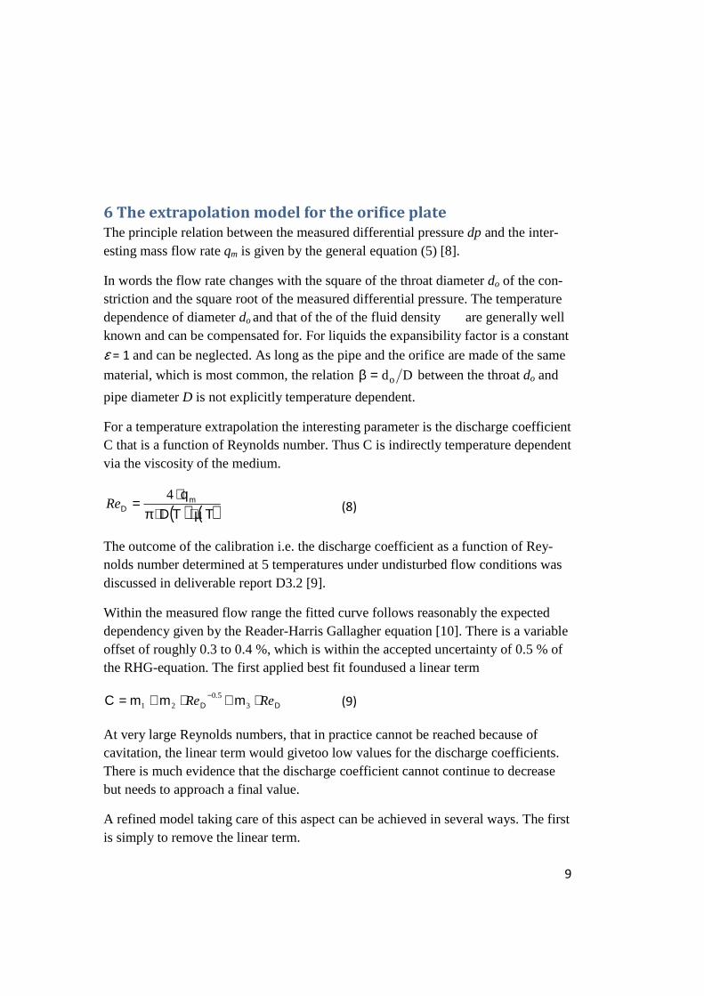
6 The extrapolation model for the orifice plate

The principle relation between the measured differential pressure dp and the inter-esting mass flow rate qm is given by the general equation (5) [8].

In words the flow rate changes with the square of the throat diameter do of the con-striction and the square root of the measured differential pressure. The temperature dependence of diameter do and that of the of the fluid density ��are generally well known and can be compensated for. For liquids the expansibility factor is a constant

ε = 1 and can be neglected. As long as the pipe and the orifice are made of the same

material, which is most common, the relation Ddo=β between the throat do and

pipe diameter D is not explicitly temperature dependent.

For a temperature extrapolation the interesting parameter is the discharge coefficient C that is a function of Reynolds number. Thus C is indirectly temperature dependent via the viscosity of the medium.

(8)

The outcome of the calibration i.e. the discharge coefficient as a function of Rey-nolds number determined at 5 temperatures under undisturbed flow conditions was discussed in deliverable report D3.2 [9].

Within the measured flow range the fitted curve follows reasonably the expected dependency given by the Reader-Harris Gallagher equation [10]. There is a variable offset of roughly 0.3 to 0.4 %, which is within the accepted uncertainty of 0.5 % of the RHG-equation. The first applied best fit foundused a linear term

(9)

At very large Reynolds numbers, that in practice cannot be reached because of cavitation, the linear term would givetoo low values for the discharge coefficients. There is much evidence that the discharge coefficient cannot continue to decrease but needs to approach a final value.

A refined model taking care of this aspect can be achieved in several ways. The first is simply to remove the linear term.

( ) ( )TTDqm

D µ⋅⋅π⋅

=4

Re

DD mmmC ReRe . ⋅+⋅+= −3

5021

10

Refined model 1: (10)

The second model would be to exchange the linear term with a different one.

Refined model 2: (11)

The third approach is to use the priciple RHG-equation model using the different Reynolds number terms with their respective exponents [2]. This equation contains totally four terms containing the pipe Reynoldsnumber ReD. However, for an orifice with corner tapping the fitting of the experimental data can be compressed to

Refined model 3: (12)

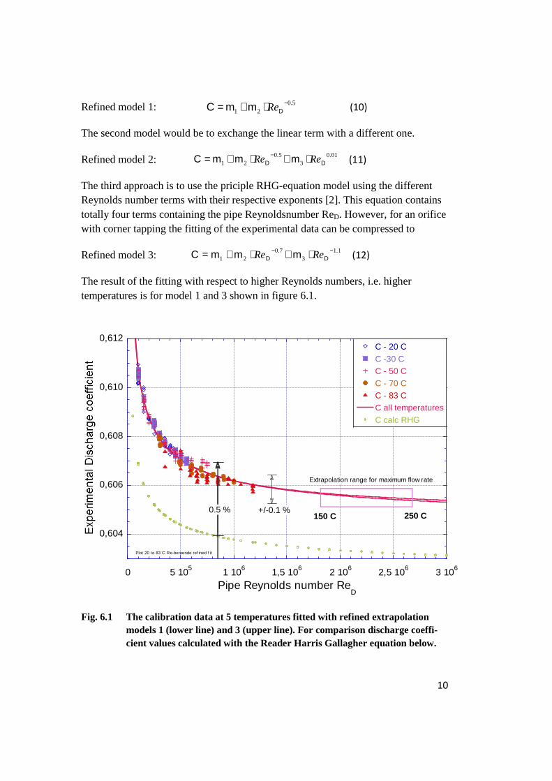
The result of the fitting with respect to higher Reynolds numbers, i.e. higher temperatures is for model 1 and 3 shown in figure 6.1.

Fig. 6.1 The calibration data at 5 temperatures fitted with refined extrapolation models 1 (lower line) and 3 (upper line). For comparison discharge coeffi-cient values calculated with the Reader Harris Gallagher equation below.

5021

.Re −⋅+= DmmC

0103

5021

.. ReRe DD mmmC ⋅+⋅+= −

113

7021

.. ReRe −− ⋅+⋅+= DD mmmC

0,604

0,606

0,608

0,610

0,612

0 5 105 1 106 1,5 106 2 106 2,5 106 3 106

C - 20 C

C -30 CC - 50 C

C - 70 CC - 83 C

C all temperatures

C calc RHG

Pipe Reynolds number ReD

Plot 20 to 83 C Re-beroende ref ined f it

Extrapolation range for maximum flow rate

150 C 250 C+/-0.1 %0.5 %

11

These fits follow well the curvature of the expected dependence according to the standard. Except these three approaches the refined model 1 was also tested with exponents -0.4 and -0,6 for ReD leading to very comparable values in the interesting temperature range of 150 to 250 °C (corresponding to a Reynoldsnumber of 1.8 to 2.7*106). The refined model 3 seems to be the most resonable one, because it reflects the experience from high Reynolds numbers and it is further valid for all types of standardised orifice plates, not only corner tappings. Thus the suggestion is to adopt the refined model 3 as the most suitable one for temperature extension purposes. The corresponding coefficient are collected in table 6.1

Table 6.1 Fitting coefficients for a refined extrapolation model – undisturbed flow

yD

xD mmmC ReRe 210 +⋅+= v

Dz

D mm ReRe 43 ++

Model 1 2 3 3 general

Exponent x

Exponent y

Exponent z

Exponent v

-0.5 -0.5

0.01

-0.7

-1.1

-0.3

-0.7

-0.8

-1.1

Coefficient m0

Coefficient m1

Coefficient m2

Coefficient m3

Coefficient m4

0.6040972

2.086789

-

0.6593323

1.524957

-0.04772729

-

-

0.6046178

28.51499

-930.8763

-

-

0.602756

0.19303

5.10305

-0.001

53.451

Difference from model 3 at ReD = 2 500 000

-0.01 % -0.18 % - -0.04 %

Besides the mentioned approches otehr exponent combinations have been tested too. As the data behaves so nice small variations in the exponents achieve quite similar calculation results for C including the general model 3 with four ReD-terms. This also means the extrapolation is not so critical. Figure 6.2 displayes six curvatures that all fit the data with almost the same quality (correlation coefficient). Several of them differ less than 0.1 % from model 3 even at very high reynolds numbers. Thus the extrapolation should not add sincere uncertainty to the experimental data having a calibration uncertainty of ±0,1 %.

12

Fig. 6.2 Seven varying approaches to fit the calibration data according to the basic form C=m0+m1ReD

x+m2ReDy and the resulting curvature of the calculated

discharge coefficient C for high Reynolds numbers.

The ISO-5167 standard [10] also treats the situation where no ideal profile can be expected. The Reader-Harris Gallager equation is still recommended for determining the discharge coefficient suggesting C decreases with increasing Reynolds number. But extra uncertainty is added to the basic one of 0.5 %.

The test program also contained a test if the extrapolation model can be used when the demands for an ideal flow profile is violated. Figure 6.3 displays the calibration results after a sincere flow disturbance achieved by an asymmetric swirl generator. In contrast to the undisturbed case the discharge coefficient now increases with increasing Reynolds number. In fact the Reader Harris Gal-lagher equation cannot be applied for this conditions. However, as shown in figure 6.3 the same refined extrapolation model is also able to fit the disturbed measurement. Due to the larger spread caused by the swirl generator the fit is not as good as in the undisturbed case. Again model 3 using the exponents ac-cording to Reader Harris Gallagher shows the most reasonable form for the extrapolation. This is a strong argument for the technique to calibrate at rea-

0,603

0,604

0,605

0,606

0,607

0,608

0,609

0,610

0,611

0 1 106

2 106

3 106

4 106

x=-0.4x=-0.5x=-0.6x=-0.7; y=-1.1x=-0.5; y=1x=-0.5; y=0.01x=-0.3; y=-0.7; z=-0.8; v=1.1

Reynolds number

+/- 0.1%

13

sonable laboratory temperatures and use the fitted equation for temperature expansion purposes.

Fig. 6.3 The measured discharge coefficient at 5 temperatures from 20 to 85°C and several flow rates at each temperature and an disturbing asym-metric swirl generator in front.

Table 6.2 contains the coefficients found for the three fitting models with model 3 as the most suitable one.

Table 6.2 Fitting coefficients for are fined extrapolation model – disturbed flow

yD

xD mmmC ReRe 210 +⋅+=

Refined fitting model 1 2 3

Exponent x

Exponent y

-0.5 -0.5

0.01

-0.7

-1.1

Coefficient m0

Coefficient m1

Coefficient m2

0.6195355

-0.8410177

-

0.5534742

-0.3857435

0.05736015

0.6194499

-12.16081

309.7903

Difference from model 3

at ReD = 2 500 000 -0.01 % 0.10 % -

0,610

0,612

0,614

0,616

0,618

0,620

0,622

4 105 8 105 1,2 106 1,6 106 2 106 2,4 106 2,8 106

Cas - 20C1

Cas - 20C2

Cas - 30C1

Cas - 30C2

Cas - 50C1

Cas - 50C2

Cas - 70C1

Cas - 70C2

Cas - 85C1

Cas - 85C2

all temperatures

Pipe Reynolds number ReD

5 temp o virvelskiva 12 D uppströms

+/- 0.1 %

model 1

model 3

model 2

14

Again the difference between the three models is relative small even at high Reynolds numbers. A conclusion of this is that the temperature extrapolation does not add much extra uncertainty to that of the calibration it self.

7 Scaling and validity of extrapolation

Meters cannot be calibrated at conditions typical for feed water in power plants. In specifying measurement uncertainties suppliers of flow meters need to allow for possible errors that cannot be tested experimentally. These uncertainties must take into consideration the various parameters involved (spread in machining, reproduci-bility, pressure and temperature effects as well as unknown dynamic interactions with medium and pipe work etc. at working conditions) with maximum uncertainty contributions combined linearly not in a statistic way.

In four cases with four different meters it could be shown that extrapolation to tem-peratures higher than 90°C is possible and leads to improved flow metering even at conditions beyond those achieved in laboratory. In calibration, even if the interest-ing flow conditions cannot fully be reached, the effect of several of these parameters can be determined under such conditions that an extrapolation is possible and rea-sonable.

However, the meters tested in this project were much smaller than those installed in power plants. Does this mean the results are only valid for the tested meters on an individual basis? Of course the extrapolations based on the coefficients found for the fitting are only valid for the individual meters. The important conclusion, how-ever, is the following. It has been shown possible to produce fully developed flow conditions and to calibrate with the temperature as a direct or indirect independent variable. Thus some of the uncertainties like spread in manufacturing and repro-ducibility could be drastically reduced. The range of data was such that all meters could be fitted with a really simple or reasonable simple model equation. These equations all behaved in a smooth and monotone way so that extrapolation to higher temperature is reasonably well predictable without adding much extra uncertainty.

The four meters, perhaps with the exception of the magnetic inductive meter, can be scaled up easily, which means characteristic measures like diameters etc. will be different but the extrapolation models as such will still hold. As a consequence the work performed in this work package can be repeated with larger meters and the same fitting and extrapolation procedure can be applied on the calibration data achieved. A further conclusion is that if high Reynolds numbers cannot be achieved by increased temperature they can be realized with increased flow rate. This is probably the closest one can come up to concerning traceability in flow at feed wa-ter conditions.

15

16

References:

[1] Set of calibration data on project web site http://www.ptb.de/emrp/ppe-

home.html

[2] Büker, O. et al : Investigations on flow meters used for accurate feed water flow

measurement , Flow Measurement and Instrumentation, 2013. Current status:

submitted.

[3] Gersten, K.: Fully developed turbulent pipe flow. In: Merzkirch, W.: Fluid Me-

chanics of Flow Metering. 1. Aufl., Springer Verlag, Berlin Heidelberg New York

2004.

[4] Dues, M.; Müller, U.: Measurements of flow profiles and characteristic num-

bers for flow conditions on test benches. Meeting of WELMEC WG 11 – Sub

Working group Water and Heat, Braunschweig, Januar 2007.

[5] Müller, U.: Richtlinie zur strömungstechnischen Validierung von Kalibrier-

Prüfständen im Rahmen der EN 1434. Deutsche Fassung, März 2007.

[6] Tawackolian K, Büker O, Hogendoorn J, Lederer T. Calibration of an ultrasonic

flow meter for hot water. Flow Measurement and Instrumentation

2013;30(0):166 -73.

[7] Tawackolian K, Büker O, Hogendoorn J, Lederer T. Investigation of a 10-path

ultrasonic flow meter for accurate feed water measurements. Measurement

Science and Technology 2013; status: submitted.

[8] SS-EN ISO 5167. Measurement of fluid flow by means of pressure differential

devices inserted in circular cross-section conduits running full – Part 1: General

principles and requirements. 2003

[9] Deliverable report D3.2 EMRP-06 Metrology for improved Power Plant Effi-

ciency. Work package 3 - Temperature extrapolation for flow meters beyond

90 °C – undisturbed and disturbed.

[10] SS-EN ISO 5167. Measurement of fluid flow by means of pressure differential

devices inserted in circular cross-section conduits running full – Part 2: Orifice

plates. 2003.

[11] SS-EN ISO 5167. Measurement of fluid flow by means of pressure differential

devices inserted in circular cross-section conduits running full – Part 4: Venturi

tubes. 2003.