sulfur chemistry in the middle atmosphere of venussulfur chemistry in the middle atmosphere of venus...

Icarus 217 (2012) 714–739

Contents lists available at ScienceDirect

Icarus

journal homepage: www.elsevier .com/ locate/ icarus

Sulfur chemistry in the middle atmosphere of Venus

Xi Zhang a,⇑, Mao Chang Liang b,c,d, Franklin P. Mills e,f, Denis A. Belyaev g,h, Yuk L. Yung a

a Division of Geological and Planetary Sciences, California Institute of Technology, Pasadena, CA 91125, USAb Research Center for Environmental Changes, Academia Sinica, Taipei, Taiwanc Graduate Institute of Astronomy, National Central University, Zhongli, Taiwand Institute of Astronomy and Astrophysics, Academia Sinica, Taipei, Taiwane RSPE/AMPL, Mills Rd., Australian National University, Canberra, ACT 0200, Australiaf Fenner School of Environment and Society, Australian National University, Canberra, ACT 0200, Australiag LATMOS, CNRS/INSU/IPSL, Quartier des Garennes, 11 bd. d’Alembert, 78280 Guyancourt, Franceh Space Research Institute (IKI), 84/32 Profsoyuznaya Str., 117997 Moscow, Russia

a r t i c l e i n f o a b s t r a c t

Article history:Available online 14 July 2011

Keywords:Venus, AtmosphereAtmospheres, ChemistryPhotochemistryAtmospheres, Composition

0019-1035/$ - see front matter � 2011 Elsevier Inc. Adoi:10.1016/j.icarus.2011.06.016

⇑ Corresponding author.E-mail address: [email protected] (X. Zhang).

Venus Express measurements of the vertical profiles of SO and SO2 in the middle atmosphere of Venusprovide an opportunity to revisit the sulfur chemistry above the middle cloud tops (�58 km). A onedimensional photochemistry-diffusion model is used to simulate the behavior of the whole chemical sys-tem including oxygen-, hydrogen-, chlorine-, sulfur-, and nitrogen-bearing species. A sulfur source isrequired to explain the SO2 inversion layer above 80 km. The evaporation of the aerosols composed of sul-furic acid (model A) or polysulfur (model B) above 90 km could provide the sulfur source. Measurementsof SO3 and SO (a1D ? X3R-) emission at 1.7 lm may be the key to distinguish between the two models.

� 2011 Elsevier Inc. All rights reserved.

1. Introduction

Venus is a natural laboratory of sulfur chemistry. Due to the dif-ficulty of observing the lower atmosphere, we are still far fromunveiling the chemistry at lower altitudes (Mills et al., 2007). Onthe other hand, the relative abundance of data above the middlecloud tops (�58 km) allows us to test the sulfur chemistry in themiddle atmosphere. Mills et al. (2007) summarized the importantobservations before Venus Express and gave an extensive review ofthe sulfur chemistry on Venus.

Recently, measurements of Venus Express and ground-basedobservations have greatly improved our knowledge of the sulfurchemistry. Marcq et al. (2005, 2006, 2008) reported the latitudinaldistributions of CO, OCS, SO2 and H2O in the 30–40 km region. Theanti-correlation of latitudinal profiles of CO and OCS implies theconversion of OCS to CO in the lower atmosphere (Yung et al.,2009). Using the latitudinal and vertical temperature distributionobtained by Pätzold et al. (2007), Piccialli et al. (2008) deducedthe dynamic structure, which shows a weak zonal wind patternabove �70 km. The discovery of the nightside warm layer by theSpectroscopy for Investigation of Characteristics of the Atmosphereof Venus (SPICAV) onboard Venus Express (Bertaux et al., 2007) is astrong evidence of substantial heating in the lower thermosphere(above 90 km). Near the antisolar point, this heating is consistentwith the existence of a subsolar–antisolar (SSAS) circulation. How-

ll rights reserved.

ever, the nightside warm layer has been reported in SPICAV obser-vations at all observed local times and latitudes and does notappear to be consistent with ground-based submillimeter observa-tions (Clancy et al., 2008). Through the occultation technique, SolarOccultation at Infrared (SOIR) and SPICAV carry out measurementsof the vertical profiles of major species above 70 km, includingH2O, HDO, HCl, HF (Bertaux et al., 2007), CO (Vandaele et al.,2008), SO and SO2 (Belyaev et al., 2008, 2012). Aerosols are foundto be in a bimodal distribution above 70 km (Wilquet et al., 2009).These high vertical resolution profiles are obtained mainly in thepolar region. Using the SPICAV nadir mode, Marcq et al. (2011a)found large temporal and spatial variations of the SO2 columndensities above the cloud top in the period of 2006–2007, whichsuggests that the cloud region is dynamically very active.Ground-based measurements also provide valuable information.Krasnopolsky (2010a, 2010b) obtained spatially resolved distribu-tions of CO2, CO, HDO, HCl, HF, OCS, and SO2 at the cloud tops fromthe CSHELL spectrograph at NASA/IRTF. Sandor et al. (2010) re-ported ground-based submillimeter observations of SO and SO2

inversion layers above 85 km. The submillimeter results are quali-tatively consistent with the vertical profiles from Venus Express(Belyaev et al., 2012). However, only the smallest SO and SO2 abun-dances inferred from the SPICAV observations (Belyaev et al., 2012)are quantitatively similar to those inferred from the submillimeterobservations (Sandor et al., 2010). Spatial and temporal variabilitymay explain at least some of the differences among the observa-tions (Sandor et al., 2010), but detailed inter-comparisons are re-quired. These measurements and the proposed correlation of

http://dx.doi.org/10.1016/j.icarus.2011.06.016

mailto:[email protected]

http://dx.doi.org/10.1016/j.icarus.2011.06.016

http://www.sciencedirect.com/science/journal/00191035

http://www.elsevier.com/locate/icarus

X. Zhang et al. / Icarus 217 (2012) 714–739 715

upper mesosphere SO2 abundances with temperature open up newopportunities to study the photochemical and transport processesin the middle atmosphere of Venus.

Sandor et al. (2010) found that SO and SO2 inversion layers can-not be reproduced by the previous photochemical model (Yungand DeMore, 1982). Therefore they suggested that the photolysisof sulfuric acid aerosol might directly produce the gas phase SOx.A detailed photochemical simulation by Zhang et al. (2010)showed that the evaporation of H2SO4 aerosols with subsequentphotolysis of H2SO4 vapor could provide the major sulfur sourcein the lower thermosphere if the rate of photolysis of H2SO4 vaporis sufficiently high. Their models also predicted supersaturation ofH2SO4 vapor pressure around 100 km. The latest SO and SO2 pro-files retrieved from the Venus Express measurements agree withtheir model results (Belyaev et al., 2012). This mechanism revealsthe close connection between the gaseous sulfur chemistry andaerosols. Previously sulfuric acid was considered only as the ulti-mate sink of gaseous sulfur species in the middle atmosphere. Ifit could also be a source, the thermodynamics and microphysicalproperties of H2SO4 must be examined more carefully. Alterna-tively, if the polysulfur (Sx) is indeed a significant component ofthe aerosols as the unknown UV absorber, Carlson (2010) esti-mated that the elemental sulfur is about 1% of the H2SO4 abun-dance. This might also be enough to produce the sulfur species ifthere is a steady supply of Sx aerosols to the upper atmosphere.

The purpose of this paper is to use photochemical models toinvestigate the sulfur chemistry in the middle atmosphere andits relation with aerosols based on our current knowledge of obser-vational evidence and laboratory measurements. We will intro-duce our model in Section 2. In Section 3, we will discuss thetwo possible sulfur sources above 90 km, H2SO4 and Sx, respec-tively, the roles they play in the sulfur chemistry, their implicationsand how to distinguish the two sources by the future observations.The last section provides a summary of the paper and conclusions.

2. Model description

Our photochemistry-diffusion model is based on the onedimensional Caltech/JPL kinetics code for Venus (Yung and De-More, 1982; Mills, 1998) with updated chemical reactions. Themodel solves the coupled continuity equations with chemicalkinetics and diffusion processes, as functions of time and altitudefrom 58 to 112 km. The atmosphere is assumed to be in hydrostaticequilibrium. We use 32 altitude grids with increments of 0.4 kmfrom 58 to 60 km and 2 km from 60 to 112 km. The diurnally aver-aged radiation field from 100 to 800 nm is calculated using a mod-ified radiative transfer scheme including gas absorption, Rayleighscattering by molecules and Mie scattering by aerosols with wave-length-dependent optical properties (see Appendix A). The un-known UV absorber is approximated by changing the singlescattering albedo of the mode 1 aerosols beyond 310 nm, as sug-gested by Crisp (1986). Because the SO, SO2 and aerosol profilesfrom Venus Express are observed in the polar region during the so-lar minimum period (2007–2008), our calculations are set at a cir-cumpolar latitude (70�N) and we use the low solar activity solarspectra for the duration of the Spacelab 3 ATMOS experiment withan overlay of Lyman alpha as measured by the Solar MesosphericExplorer (SME).

In this study we selected 51 species, namely, O, O(1D), O2,O2(1D), O3, H, H2, OH, HO2, H2O, H2O2, N2, Cl, Cl2, ClO, HCl, HOCl,ClCO, COCl2, ClC(O)OO, CO, CO2, S, S2, S3, S4, S5, S7, S8, SO, (SO)2,SO2, SO3, S2O, HSO3, H2SO4, OCS, OSCl, ClSO2, four chlorosulfanes(ClS, ClS2, Cl2S, and Cl2S2) and eight nitrogen-containing species(N, NO, NO2, NO3, N2O, HNO, HNO2, and HNO3). The chlorosulfanes(SmCln) are included because they open an important pathway to

form S2 and polysulfur Sx(x=2?8) in the region 60–70 km (Millsand Allen, 2007), although there are significant uncertainties intheir chemistry. The chlorosulfane chemistry is not important forthe sulfur cycles above �80 km because the SmCln abundancesare low. Nitrogen-containing species, especially NO and NO2, canact as catalysts for converting SO to SO2 and O to O2 in the 70–80 km region (Krasnopolsky, 2006). A recent study by Sundaramet al. (2011) suggests that the odd nitrogen (NOx) chemistry mightalso have significant effects on the abundances of sulfur oxides inthe 80–90 km region.

In Zhang et al. (2010), the chemistry was simplified because(SO)2, S2O and HSO3 were considered only as the sinks of the sulfurspecies. This might not be accurate enough for the chemistry below80 km where there seems to be difficulty in matching the SO2

observations. Instead, a full set of 41 photodissociation reactionsis used here, along with about 300 neutral chemical reactions, aslisted in Tables 1 and 2 respectively. We take the ClCO thermalequilibrium constant from the 1-sigma model in Mills et al.(2007) so that we can constrain the total O2 column abundancesto �2 � 1018 cm�2. In addition, we introduce the heterogeneousnucleation processes of elemental sulfur (S, S2 and polysulfur) be-cause these sulfur species can readily stick to sulfuric acid dropletsand may provide the source material for the unknown UV absorber(Carlson, 2010). But we neglect all the heterogeneous reactionsamong the condensed elemental sulfur species on the droplet sur-face. The calculation of the heterogeneous condensation rates isdescribed in Appendix B. The accommodation coefficient a is var-ied from 0.01 to 1 for the sensitivity study (Section 4).

The temperature profiles are shown in Fig. 1 (left panel). Thedaytime temperature profile below 100 km (solid line) is obtainedfrom the observations of VeRa onboard Venus Express near the po-lar region (71�N, Fig. 1 of Pätzold et al., 2007). Above 100 km thetemperature is from Seiff (1983). The nighttime temperature pro-file (dashed line) above 90 km is measured by Venus Express in or-bit 104 at latitude 4�S and local time 23:20 h (black curve in Fig. 1of Bertaux et al. (2007)). The nighttime temperature profile is usedto calculate the H2SO4 saturation vapor pressure only.

In the 1-D model, species are assumed to be mixed vertically byturbulent eddies. Molecular diffusion becomes important abovethe homopause region (�130–135 km). The eddy diffusivity in-creases with altitude in the Venus mesosphere for reasons dis-cussed later. Since the zonal wind is observed to decrease withaltitude above 70 km due to the temperature gradient from poleto equator (Piccialli et al., 2008), we assume that vertical transportof gas species is predominantly due to mixing caused by transientinternal gravity waves, as proposed by Prinn (1975). In this casethe eddy diffusion coefficient will be inversely proportional tothe square root of the number density (Lindzen, 1981). Von Zahnet al. (1980) derived the eddy diffusion coefficient�1.4 � 1013 [M]�0.5 cm2 s�1 from the number density around thehomopause region, based on mass spectrometer measurementsfrom Pioneer Venus. In our model we use slightly larger valuesKz = 2.0 � 1013 [M]�0.5 cm2 s�1 above 80 km to include an addi-tional contribution of the SSAS circulation. In the region below80 km, Woo and Ishimaru (1981) estimated the diffusivity64.0 � 104 cm2 s�1 at �60 km from radio signal scintillations.Therefore our eddy diffusivity profile from 58 to 80 km is esti-mated by linear interpolation between the values at 80 and60 km. The eddy diffusion profile is shown in Fig. 1 (right panel).However, the vertical advection due to the SSAS circulation mightbe dominant above 90 km. The SPICAV measurements show thatthe SO2 mixing ratio from �90 to 100 km is almost constant withaltitude, which implies a very efficient transport process.

Since Zhang et al. (2010) has already shown that the modelwithout additional sulfur sources above 90 km cannot explainthe observed SO2 inversion layer, we focus on two models in this

Table 1Photolysis reactions.

Reaction Photolysis coefficient J (s�1) Wavelength (nm) Reference

at 112 km at 68 km

R1 O2 + ht ? 2O 8.8 � 10�8 7.4 � 10�10 3 6 k 6 242 bR2 O2 + ht ? O + O(1D) 2.1 � 10�7 0 117 6 k 6 178 bR3 O3 + ht ? O2 + O 1.2 � 10�3 2.3 � 10�3 158 6 k 6 800 aR4 O3 + ht ? O2(1D) + O(1D) 7.6 � 10�3 1.1 � 10�2 53 6 k 6 325 aR5 O3 + ht ? O2 + O(1D) 2.3 � 10�6 3.2 � 10�6 320 6 k 6 325 aR6 O3 + ht ? O2(1D) + O 2.6 � 10�6 3.2 � 10�6 120 6 k 6 325 aR7 O3 + ht ? 3O 9.2 � 10�7 1.0 � 10�11 53 6 k 6 203 aR8 OH + ht ? O + H 4.8 � 10�6 0 91 6 k 6 193 dR9 HO2 + ht ? OH + O 5.4 � 10�4 7.0 � 10�4 190 6 k 6 260 cR10 H2O + ht ? H + OH 3.1 � 10�6 0.0 61 6 k 6 198 aR11 H2O + ht ? H2 + O(1D) 5.2 � 10�8 0.0 80 6 k 6 143 aR12 H2O + ht ? 2H + O 6.2 � 10�8 0.0 80 6 k 6 143 aR13 H2O2 + ht ? 2OH 9.7 � 10�5 1.3 � 10�4 120 6 k 6 350 aR14 Cl2 + ht ? 2Cl 2.6 � 10�3 3.9 � 10�3 240 6 k 6 475 aR15 ClO + ht ? Cl + O 6.2 � 10�3 8.4 � 10�3 230 6 k 6 325 aR16 HCl + ht ? H + Cl 1.9 � 10�6 5.5 � 10�8 135 6 k 6 232 eR17 HOCl + ht ? OH + Cl 4.6 � 10�4 6.4 � 10�4 200 6 k 6 380 aR18 COCl2 + ht ? 2Cl + CO 5.1 � 10�5 7.4 � 10�5 182 6 k 6 285 aR19 CO2 + ht ? CO + O 1.1 � 10�8 4.3 � 10�13 120 6 k 6 204 aR20 CO2 + ht ? CO + O(1D) 3.5 � 10�9 0.0 63 6 k 6 160 aR21 S2 + ht ? 2S 4.0 � 10�3 5.8 � 10�3 238 6 k 6 278 bR22 S3 + ht ? S2 + S 1.2 2.4 350 6 k 6 455 bR23 S4 + ht ? 2S2 2.2 � 10�1 5.5 � 10�1 425 6 k 6 575 bR24 ClS + ht ? S + Cl 2.6 � 10�2 59 � 10�2 337 6 k 6 500 aR25 Cl2S + ht ? ClS + Cl 2.2 � 10�3 3.9 � 10�3 190 6 k 6 460 aR26 ClS2 + ht ? S2 + Cl 6.8 � 10�2 1.4 � 10�1 327 6 k 6 485 aR27 SO + ht ? S + O 3.7 � 10�4 1.8 � 10�4 113 6 k 6 232 aR28 SO2 + ht ? S + O2 1.5 � 10�6 1.9 � 10�7 63 6 k 6 210 a*

R29 SO2 + ht ? SO + O 2.0 � 10�4 7.2 � 10–5 63 6 k 6 220 aR30 SO3 + ht ? SO2 + O 3.6 � 10�5 3.7 � 10�5 195 6 k 6 300 fR31 OCS + ht ? CO + S 2.8 � 10�5 4.2 � 10�5 185 6 k 6 300 aR32 H2SO4 + ht ? SO3 + H2O 1.4 � 10�6 1.4 � 10�7 121 6 k 6 746 g, h, i, j, kR33 S2O + ht ? SO + S 5.0 � 10�2 6.2 � 10�2 260 6 k 6 335 aR34 ClC(O)OO + ht ? CO2 + ClO 5.3 � 10�3 7.4 � 10�3 205 6 k 6 305 lR35 NO + ht ? N + O 4.3 � 10�6 0.0 175 6 k 6 195 mR36 NO2 + ht ? NO + O 8.6 � 10�3 1.5 � 10�2 120 6 k 6 422 mR37 NO3 + ht ? NO2 + O 1.6 � 10�1 4.4 � 10�1 410 6 k 6 645 nR38 NO3 + ht ? NO + O2 2.4 � 10�2 6.3 � 10�2 590 6 k 6 645 nR39 N2O + ht ? N2 + O(1D) 8.9 � 10�7 3.0 � 10�3 100 6 k 6 240 mR40 HNO2 + ht ? OH + NO 1.9 � 10�3 8.7 � 10�3 310 6 k 6 390 mR41 HNO3 + ht ? NO2 + OH 1.2 � 10�4 5.2 � 10�5 190 6 k 6 350 m

Note: The photolysis coefficient (J) in the units of s�1refers to 112 km and 68 km at mid-latitude (45�N) with diurnal average (divided by 2).References: (a) Mills (1998) and references therein; (b) Moses et al. (2002) and references therein; (c) Sander et al. (2006) and references therein; (d) Moses et al. (2000) andreferences therein; (e) Bahou et al. (2001); (f) Burkholder and McKeen (1997); (g) Vaida et al. (2003); (h) Mills et al. (2005); (i) Burkholder et al. (2000); (j) Hintze et al. (2003);(k) Lane and Kjaergaard (2008); (l) Pernice et al. (2004); (m) DeMore et al. (1994) and references therein; (n) DeMore et al. (1997) and references therein.* Total SO2 absorption cross sections between 227 and 420 nm are updated based on recent measurements by Hermans et al. (2009) and Vandaele et al. (2009).

Table 2Chemical reactions.

Reaction Rate constant Reference

R50 O(1D) + O2 ? O + O2 3.20 � 10�11e70./T cR51 O(1D) + N2 ? O + N2 1.80 � 10�11e110./T cR52 O(1D) + CO2 ? O + CO2 7.40 � 10�11e120./T cR53 O2(1D) + O ? O2 + O 2.00 � 10�16 cR54 O2(1D) + O2 ? 2O2 3.60 � 10�18e�220./T cR55 O2(1D) + H2O ? O2 + H2O 4.80 � 10�18 cR56 O2(1D) + N2 ? O2 + N2 1.00 � 10�20 cR57 O2(1D) + CO ? O2 + CO 1.00 � 10�20 aR58 O2(1D) + CO2 ? O2 + CO2 2.00 � 10�21 EstimatedR59 2O + CO2 ? O2 + CO2 k0 = 3.22 � 10�28T�2.0 EstimatedR60 2O + CO2 ? O2(1D) + CO2 k0 = 9.68 � 10�28T�2.0 EstimatedR61 2O + O2 ? O3 + O k0 = 5.90 � 10�34(T/300.)�2.4 a

k1 = 2.80 � 10�12

R62 O + 2O2 ? O3 + O2 k0 = 5.90 � 10�34(T/300.)�2.4 ak1 = 2.80 � 10�12

R63 O + O2 + N2 ? O3 + N2 k0 = 5.95 � 10�34(T/300.)�2.3 ak1 = 2.80 � 10�12

R64 O + O2 + CO ? O3 + CO k0 = 6.70 � 10�34(T/300.)�2.5 ak1 = 2.80 � 10–12

716 X. Zhang et al. / Icarus 217 (2012) 714–739

Table 2 (continued)


R65 O + O2 + CO2 ? O3 + CO2 k0 = 1.40 � 10�33(T/300.)�2.5 ak1 = 2.80 � 10�12

R66 H + O2 + N2 ? HO2 + N2 k0 = 5.70 � 10�32(T/300.)�1.6 ck1 = 7.50 � 10�11

R67 O + O3 ? 2O2 8.00 � 10�12e�2060./T cR68 O(1D) + O3 ? 2O2 1.20 � 10�10 cR69 O(1D) + O3 ? 2O + O2 1.20 � 10�10 cR70 O2(1D) + O3 ? 2O2 + O 5.20 � 10�11e�2840./T cR71 H + O3 ? OH + O2 1.40 � 10�10e�470./T cR72 OH + O3 ? HO2 + O2 1.70 � 10�12e�940./T cR73 OH + O3 ? HO2 + O2(1D) 3.20 � 10�14e�940./T aR74 HO2 + O3 ? OH + 2O2 1.00 � 10�14e�490./T cR75 O + H + M ? OH + M k0 = 1.30 � 10�29T�1.0 gR76 2H + M ? H2 + M k0 = 2.70 � 10�31T�0.6 dR77 O + H2 ? OH + H 8.50 � 10�20T2.7e�3160./T dR78 O(1D) + H2 ? H + OH 1.10 � 10�10 cR79 OH + H2 ? H2O + H 5.50 � 10�12e�2000./T cR80 O + OH ? O2 + H 2.20 � 10�11e120./T cR81 H + OH + N2 ? H2O + N2 k0 = 6.10 � 10�26T�2.0 dR82 H + OH + CO2 ? H2O + CO2 k0 = 7.70 � 10�26T�2.0 dR83 2OH ? H2O + O 4.20 � 10�12e�240./T cR84 2OH + M ? H2O2 + M k0 = 6.20 � 10�31(T/300.)�1.0 c

k1 = 2.60 � 10�11

R85 O + HO2 ? OH + O2 3.00 � 10�11e200./T cR86 O + HO2 ? OH + O2(1D) 6.00 � 10�13e200./T aR87 H + HO2 ? 2OH 7.21 � 10�11 cR88 H + HO2 ? H2 + O2 7.29 � 10�12 cR89 H + HO2 ? H2 + O2(1D) 1.30 � 10�13 aR90 H + HO2 ? H2O + O 1.62 � 10�12 cR91 OH + HO2 ? H2O + O2 4.80 � 10�11e250./T cR92 OH + HO2 ? H2O + O2(1D) 9.60 � 10�13e250./T cR93 2HO2 ? H2O2 + O2 2.30 � 10�13e600./T cR94 2HO2 ? H2O 2 + O2(1D) 4.60 � 10�15e600./T EstimatedR95 2HO2 + M ? H2O 2 + O2 + M k0 = 1.70 � 10�33e1000./T cR96 O(1D) + H2O ? 2OH 2.20 � 10�10 cR97 O + H2O2 ? OH + HO2 1.40 � 10�12e�2000./T cR98 OH + H2O2 ? H2O + HO2 2.90 � 10�12e�160./T cR99 Cl + O + M ? ClO + M k0 = 5.00 � 10�32 eR100 Cl + O3 ? ClO + O2 2.30 � 10�11e�200./T cR101 Cl + O3 ? ClO + O2(1D) 5.80 � 10�13e�260./T cR102 Cl + H + M ? HCl + M k0 = 1.00 � 0�32 eR103 Cl + H2 ? HCl + H 3.70 � 10�11e�2300./T cR104 Cl + OH ? HCl + O 8.33 � 10�12e�2790./T hR105 Cl + HO2 ? HCl + O2 1.80 � 10�11e170./T cR106 Cl + HO2 ? OH + ClO 4.10 � 10�11e�450./T cR107 Cl + H2O2 ? HCl + HO2 1.10 � 10�11e�980./T cR108 Cl + HOCl ? OH + Cl2 6.00 � 10�13e�130./T cR109 Cl + HOCl ? HCl + ClO 1.90 � 10�12e�130./T cR110 Cl + ClCO ? Cl2 + CO 2.16 � 10�9e�1670./T hR111 Cl + CO + N2 ? ClCO + N2 k0 = 1.30 � 10�33 (T/300.)�3.8 aR112 Cl + OCS ? ClS + CO 1.00 � 10�16 cR113 Cl + ClS2 ? S2 + Cl2 1.00 � 10�12 bR114 Cl + SO2 + M ? ClSO2 + M k0 = 1.30 � 10�34e940./T aR115 2Cl + N2 ? Cl2 + N2 k0 = 6.10 � 10�34e900./T aR116 2Cl + CO2 ? Cl2 + CO2 k0 = 2.60 � 10�33e900./T aR117 O + Cl2 ? ClO + Cl 7.40 � 10�12e�1650./T aR118 O(1D) + Cl2 ? Cl + ClO 1.55 � 10�10 cR119 O(1D) + Cl2 ? Cl2 + O 5.25 � 10�11 cR120 H + Cl2 ? HCl + Cl 1.43 � 10�10e�590./T aR121 OH + Cl2 ? Cl + HOCl 1.40 � 10�12e�900./T cR122 ClCO + Cl2 ? COCl2 + Cl 6.45 � 10�12 k145 (170a+[M]) aR123 ClO + O ? Cl + O2 3.00 � 10�11e70./T cR124 ClO + O ? Cl + O2(1D) 6.00 � 10�13e70./T cR125 ClO + H2 ? HCl + OH 1.00 � 10�12e�4800./T cR126 ClO + OH ? HO2 + Cl 7.40 � 10�12e270./T cR127 ClO + OH ? HCl + O2 6.00 � 10�13e230./T cR128 ClO + HO2 ? HOCl + O2 2.70 � 10�12e220./T cR129 ClO + CO ? CO2 + Cl 1.00 � 10�12e�3700./T cR130 2ClO ? Cl2 + O2 1.00 � 10�12e�1590./T cR131 2ClO ? Cl2 + O2(1D) 2.00 � 10�14e�1590./T cR132 ClO + OCS ? OSCl + CO 2.00 � 10�16 cR133 ClO + SO ? Cl + SO2 2.80 � 10�11 cR134 ClO + SO2 ? Cl + SO3 4.00 � 10�18 cR135 ClO + SO2 + M ? Cl + SO3 + M k0 = 1.00 � 10�35 a

k1 = 4.00 � 10�19

(continued on next page)


Table 2 (continued)


R136 O + HCl ? OH + Cl 1.00 � 10�11e�3300./T cR137 O(1D) + HCl ? Cl + OH 1.00 � 10�10 cR138 O(1D) + HCl ? ClO + H 3.60 � 10�11 cR139 O(1D) + HCl ? O + HCl 1.35 � 10�11 cR140 OH + HCl ? Cl + H2O 2.60 � 10�12e�350./T cR141 O + HOCl ? OH + ClO 1.70 � 10�13 cR142 OH + HOCl ? H2O + ClO 3.00 � 10�12e�500./T cR143 O + ClCO ? Cl + CO2 3.00 � 10�11 eR144 O + ClCO ? CO + ClO 3.00 � 10�12 eR145 ClCO + O2 + M ? ClC(O)OO + M k0 = 5.70 � 10�15e500./T/(1017 + 0.05�[M]) eR146 H + ClCO ? HCl + CO 1.00 � 10�11 eR147 OH + ClCO ? HOCl + CO 1.50 � 10�10 aR148 2ClCO ? COCl2 + CO 5.00 � 10�11 aR149 ClCO + ClC(O)OO ? 2CO2 + 2Cl 1.00 � 10�11 aR150 ClCO + N2 ? CO + Cl + N2 keq = 1.60 � 10�25e4000./T aR151 O(1D) + COCl2 ? Cl2 + CO2 3.60 � 10�10 cR152 O(1D) + COCl2 ? ClCO + ClO 3.60 � 10�10 aR153 O + ClC(O)OO ? Cl + O2 + CO2 1.00 � 10�11 eR154 H + ClC(O)OO ? Cl + OH + CO2 1.00 � 10�11 eR155 Cl + ClC(O)OO ? Cl + ClO + CO2 1.00 � 10�11 eR156 2ClC(O)OO ? 2Cl + 2CO2 + O2 5.00 � 10�12 aR157 H + O2 + CO2 ? HO2 + CO2 k0 = 2.00 � 10�31(T/300.)�1.6 a

k1 = 7.50 � 10�11

R158 H + HCl ? H2 + Cl 1.50 � 10�11e�1750./T aR159 Cl + CO + CO2 ? ClCO + CO2 k0 = 4.20 � 10�33(T/300.)�3.8 aR160 ClCO + CO2 ? CO + Cl + CO2 keq = 1.60 � 10�25e4000./T aR161 O + CO + M ? CO2 + M k0 = 1.70 � 10�33e�1510./T g

k1 = 2.66 � 10�14e�1459./T

R162 O + 2CO ? CO2 + CO k0 = 6.50 � 10�33e�2180./T aR163 2O + CO ? CO2 + O k0 = 3.40 � 10�33e�2180./T aR164 OH + CO ? CO2 + H 1.50 � 10�13 cR165 S + O + M ? SO + M k0 = 1.50 � 10�34e900./T bR166 S + O2 ? SO + O 2.30 � 10�12 iR167 SO + O ? SO2 + O 1.60 � 10�13e�2280./T kR168 HSO3 + O2 HO2 + SO3 1.30 � 10�12e�330./T cR169 ClS + O2 ? SO + ClO 2.00 � 10�15 lR170 S + O3 ? SO + O2 1.20 � 10�11 cR171 SO + O3 ? SO2 + O2 4.50 � 10�12e�1170./T kR172 SO + O3 ? SO2 + O2(1D) 3.60 � 10�13e�1100./T cR173 SO2 + O3 ? SO3 + O2 3.00 � 10�12e�7000./T cR174 SO2 + O3 ? SO3 + O2(1D) 6.00 � 10�14e�7000./T EstimatedR175 S + OH ? SO + H 6.60 � 10�11 cR176 S + HO2 ? SO + OH 3.00 � 10�11e200./T eR177 SO3 + H2O ? H2SO4 2.26 � 10�43 Te�6544/T [H2O] jR178 ClS + Cl2 ? Cl2S + Cl 7.00 � 10�14 lR179 S + Cl + M ? ClS + M k0 = 1.00 � 10�29 T�1.0 bR180 S + Cl2 ? ClS + Cl 2.80 � 10�11e�290.T lR181 S + ClO ? SO + Cl 4.00 � 10�11 bR182 S + ClCO ? CO + ClS 3.00 � 10�12 EstimatedR183 S + ClCO ? OCS + Cl 3.00 � 10�12 EstimatedR184 S + ClC(O)OO ? Cl + SO + CO2 3.00 � 10�11 aR185 S + CO + M ? OCS + M k0 = 4.00 � 10�33e�1940./T EstimatedR186 2S + M ? S2 + M k0 = 1.18 � 10�29 a

k1 = 1.00 � 10�10

R187 O + S2 ? SO + S 2.20 � 10�11e�84./T bR188 S + S2 + M ? S3 + M k0 = 1.00 � 10�25T�2.0 a, b

k1 = 3.00 � 10�11

R189 ClO + S2 ? S2O + Cl 2.80 � 10�11 bR190 2S2 + M ? S4 + M k0 = 2.20 � 10�29 a

k1 = 1.00 � 10�10

R191 O + S3 ? SO + S2 8.00 � 10�11 bR192 S + S3 ? 2S2 8.00 � 10�11 bR193 S + S3 + M ? S4 + M k0 = 1.00 � 10�25T�2.0 a, b

k1 = 3.00 � 10�11

R194 S2 + S3 + M ? S5 + M k0 = 1.00 � 10�25T�2.0 a, bk1 = 3.00 � 10�11

R195 2S3 + M ? S6 + M k0 = 1.00 � 10�30 ak1 = 3.00 � 10�11

R196 O + S4 ? SO + S3 8.00 � 10�11 bR197 Cl + S4 ? ClS2 + S2 2.00 � 10�12 lR198 S + S4 ? S2 + S3 8.00 � 10�11 bR199 S3 + S4 ? S2 + S5 4.00 � 10�11e�200./T bR200 S + S4 + M ? S5 + M k0 = 1.00 � 10�25T�2.0 a, b

k1 = 3.00 � 10�11

R201 S2 + S4 + M ? + M k0 = 1.00 � 10�25T�2.0 a, b


Table 2 (continued)


k1 = 3.00 � 10�11

R202 S3 + S4 + M ? S7 + M k0 = 1.00 � 10�25T�2.0 a, bk1 = 3.00 � 10�11

R203 S4 + M ? 2S2 + M keq = 2.71 � 10�27e13100./T fR204 2S4 + M ? S8 + M k0 = 1.00 � 10�30 a

k1 = 3.00 � 10�11

R205 O + S5 ? S4 + SO 8.00 � 10�11e�200./T bR206 S + S5 ? 2S3 3.00 � 10�11e�200./T bR207 S + S5 ? S2 + S4 5.00 � 10�11e�200./T bR208 S3 + S5 ? S2 + S6 4.00 � 10�11e�200./T bR209 S4 + S5 ? S2 + S7 2.00 � 10�12e�200./T bR210 S4 + S5 ? S3 + S6 2.00 � 10�12e�200./T bR211 S + S5 + M ? S6 + M k0 = 1.00 � 10�25 T�2.0 a, b

k1 = 3.00 � 10�11

R212 S2 + S5 + M ? S7 + M k0 = 1.00 � 10�25 T�2.0 a, bk1 = 3.00 � 0�11

R213 S3 + S5 + M ? S8 + M k0 = 1.00 � 10�25T�2.0 a, bk1 = 3.00 � 10�11

R214 O + S6 ? S5 + SO 8.00 � 10�11e�300./T bR215 S + S6 ? S3 + S4 3.00 � 10�11e�300./T bR216 S + S6 ? S2 + S5 5.00 � 10�11e�300./T bR217 S3 + S6 ? S2 + S7 4.00 � 10�12e�300./T bR218 S4 + S6 ? S2 + S8 2.00 � 10�12e�300./T bR219 S4 + S6 ? 2S5 2.00 � 10�12e�300./T bR220 S + S6 + M ? S7 + M k0 = 1.00 � 10�25 T�2.0 a, b

k1 = 3.00 � 10�11

R221 S2 + S6 + M ? S8 + M k0 = 1.00 � 10�25 T�2.0 a, bk1 = 3.00 � 10�11

R222 S6 + M ? 2S3 + M keq = 2.41 � 10�29e21483./T fR223 O + S7 ? S6 + SO 8.00 � 10�11e�200./T bR224 S + S7 ? S2 + S6 4.00 � 10�11e�200./T bR225 S + S7 ? S3 + S5 2.00 � 10�11e�200./T bR226 S + S7 ? 2S4 2.00 � 10�11e�200./T bR227 S3 + S7 ? S2 + S8 3.00 � 10�11e�200./T bR228 S3 + S7 ? S4 + S6 1.00 � 10�11e�200./T bR229 S3 + S7 ? 2S5 1.00 � 10�11e�200./T bR230 S4 + S7 ? S3 + S8 5.00 � 10�12e�200./T bR231 S4 + S7 ? S5 + S6 5.00 � 10�12e�200./T bR232 S + S7 + M ? S8 + M k0 = 1.00 � 10�25 T�2.0 a, b

k1 = 3.00 � 10�11

R233 O + S8 ? S7 + SO 8.00 � 10�11e�400./T bR234 S + S8 ? S2 + S7 4.00 � 10�11e�400/T bR235 S + S8 ? S3 + S6 2.00 � 10�11e�400./T bR236 S + S8 ? S4 + S5 2.00 � 10�11e�400./T bR237 S2 + S8 ? 2S5 1.00 � 10�11e�1400./T bR238 S8 + M ? 2S4 + M keq = 1.17 � 10�29e22695./T fR239 O + SO ? S + O2 6.60 � 10�13e�2760./T aR240 O + SO + M ? SO2 + M k0 = 5.10 � 10�31 a*

k1 = 5.30 � 10�11

R241 OH + SO ? SO2 + H 8.60 � 10�11 cR242 HO2 + SO ? SO2 + OH 2.80 � 10�11 EstimatedR243 Cl + SO + M ? OSCl + M k0 = 7.30 � 10�21 T�5.0 lR244 ClC(O)OO + SO ? Cl + SO2 + CO2 1.00 � 10�11 aR245 ClS + SO ? S2O + Cl 1.00 � 10�11 bR246 S3 + SO ? S2O + S2 1.00 � 10�12 bR247 S + SO + M ? S2O + M k0 = 3.30 � 10�26 T�2.0 b*

R248 2SO ? SO2 + S 1.00 � 10�12e�1700./T bR249 2SO + M ? (SO)2 + M k0 = 4.40 � 10�31 a

k1 = 1.00 � 10�11

R250 O + (SO)2 ? S2O + O2 3.00 � 10�14 aR251 O + (SO)2 ? SO + SO2 3.00 � 10�15 aR252 S2 + (SO)2 ? 2S2O 3.30 � 10�14 aR253 SO + (SO)2 ? S2O + SO2 3.30 � 10�14 bR254 (SO)2 + M ? 2SO + M keqkeq = 1.00 � 10�28e6000./T aR255 O + SO2 ? SO + O2 8.00 � 10�12e�9800./T aR256 O(1D) + SO2 ? SO2 + O 7.00 � 10�11 bR257 O(1D) + SO2 ? SO + O2 1.30 � 10�10 bR258 O + SO2 + M ? SO3 + M k0 = 1.32 � 10�31e�1000./T k*

R259 OH + SO2 + M ? HSO3 + M k0 = 1.10 � 10�30 (T/300.)�4.3 i*

k1 = 1.60 � 10�12

R260 HO2 + SO2 ? OH + SO3 1.00 � 10�18 cR261 ClC(O)OO + SO2 ? Cl + SO3 + CO2 1.00 � 10�15 aR262 O + SO3 ? SO2 + O2 2.32 � 10�16e�487./T bR263 S + SO3 ? SO2 + SO 1.00 � 10�16 bR264 S2 + SO3 ? S2O + SO2 2.00 � 10�16 bR265 SO + SO3 ? 2SO2 2.00 � 10�15 b

(continued on next page)


Table 2 (continued)


R266 O + S2O ? 2SO 1.70 � 10�12 aR267 S + S2O ? S2 + SO 1.00 � 10�12e�1200./T bR268 2S2O ? S3 + SO2 1.00 � 10�14 aR269 O + ClS ? SO + Cl 1.20 � 10�10 lR270 Cl + ClS ? S + Cl2 1.00 � 10�14 aR271 Cl + ClS + M ? Cl2S + M k0 = 1.00 � 10�30 l

k1 = 5.00 � 10�11

R272 S + ClS ? S2 + Cl 1.00 � 10�11 lR273 S2 + ClS ? S3 + Cl 2.00 � 10�11 bR274 2ClS ? S2 + Cl2 6.00 � 10�12 lR275 2ClS ? Cl2S + S 7.50 � 10�12 aR276 2ClS ? ClS2 + Cl 5.40 � 10�11 lR277 2ClS + M ? Cl2S2 + M k0 = 4.00 � 10�31 a

k1 = 4.00 � 10�12

R278 OCS + ClS ? ClS2 + CO 3.00 � 10�16 aR279 O + ClS2 ? SO + ClS 1.00 � 10�13 bR280 Cl + ClS2 ? Cl2 + S2 1.00 � 10�11 lR281 ClS + ClS2 ? Cl2S + S2 1.00 � 10�12 aR282 H + Cl2S ? HCl + ClS 2.00 � 10�11 aR283 Cl + Cl2S ? Cl2 + ClS 1.00 � 10�19 aR284 2Cl2S ? Cl2S2 + Cl2 1.00 � 10�20 aR285 Cl + Cl2S2 ? Cl2 + ClS2 4.30 � 10�12 aR286 O + OSCl ? SO2 + Cl 5.00 � 10�11e�600./T bR287 O + OSCl ? SO + ClO 2.00 � 10�11e�600./T bR288 Cl + OSCl ? Cl2 + SO 2.30 � 10�11 lR289 S + OSCl ? S2O + Cl 5.00 � 10�11e�600./T bR290 S + OSCl ? SO + ClS 2.00 � 10�11e�600./T bR291 SO + OSCl ? SO2 + ClS 6.00 � 10�13 lR292 OSCl + M ? SO + Cl + M 7.29 � 10�21T�5.0 aR293 O + ClSO2 ? SO2 + ClO 1.00 � 10�11 aR294 H + ClSO2 ? SO2 + HCl 1.00 � 10�11 aR295 Cl + ClSO2 ? SO2 + Cl2 1.00 � 10�20 bR296 ClS + ClSO2 ? SO2 + Cl2S 5.00 � 10–12 lR297 S + ClSO2 ? SO2 + ClS 1.00 � 10�11 bR298 S2 + ClSO2 ? SO2 + ClS2 5.00 � 10�11e�800./T bR299 SO + ClSO2 ? OSCl + SO2 5.00 � 10�11e�800./T bR300 2ClSO2 ? Cl2 + 2SO2 5.00 � 10�13 bR301 O + OCS ? SO + CO 1.60 � 10�11e�2150./T kR302 S + OCS ? S2 + CO 6.63 � 10�20 T2.57e�1180./T mR303 S2 + M ? 2S + M keq = 2.68 � 10�25e50860./T fR304 N + O2 ? NO + O 1.50 � 10�11e�3600./T cR305 HNO + O2 ? NO + HO2 5.25 � 10�12e�1510./T nR306 N + O3 ? NO + O2 2.00 � 10�16 cR307 N + OH ? NO + H 3.80 � 10�11e85./T oR308 O2(1D) + N ? NO + O 9.00 � 10�17 cR309 N + HO2 ? NO + OH 2.20 � 10�11 pR310 2 N + M ? N2 + M k0 = 8.27 � 10�34e490./T qR311 O(1D) + N2 + M ? N2O + M k0 = 3.50 � 10�37 (T/300.)�0.6 cR312 O + NO + M ? NO2 + M k0 = 9.00 � 10�31 (T/300.)�1.5 c

k1 = 3.00 � 10�11

R313 O3 + NO ? NO2 + O2 3.00 � 10�12e�1500./T cR314 H + NO + M ? HNO + M k0 = 3.23 � 10�32 rR315 OH + NO + M ? HNO2 + M k0 = 7.00 � 10�31 (T/300.)�2.6 c

k1 = 3.60 � 10�11 (T/300.)�0.1

R316 HO2 + NO ? NO2 + OH 3.50 � 10�12e250./T cR317 N + NO ? N2 + O 2.10 � 10�11e100./T cR318 O + NO2 ? NO + O2 5.60 � 10�12e180./T cR319 O + NO2 + M ? NO3 + M k0 = 2.50 � 10�31 (T/300.)�1.8 c

k1 = 2.20 � 10�11(T/300.)�0.7

R320 O3 + NO2 ? NO3 + O2 1.20 � 10�13e�2450./T cR321 H + NO2 ? OH + NO 4.00 � 10�10e340./T cR322 OH + NO2 + M ? HNO3 + M k0 = 2.00 � 10�30 (T/300.)�3.0 c

k1 = 2.50 � 10�11e300./T

R323 HO2 + NO2 ? HNO2 + O2 5.00 � 10�16 cR324 N + NO2 ? N2O + O 5.80 � 10�12e220./T cR325 NO3 + NO2 ? NO + NO2 + O2 4.50 � 10�14e�1260./T cR326 O + NO3 ? O2 + NO2 1.00 � 10�11 cR327 H + NO3 ? OH + NO2 1.10 � 10�10 sR328 OH + NO3 ? HO2 + NO2 2.20 � 10�11 cR329 HO2 + NO3 ? HNO3 + O2 3.50 � 10�12 cR330 NO + NO3 ? 2NO2 1.50 � 10�11e170./T cR331 2NO3 ? 2NO2 + O2 8.50 � 10�13e2450./T cR332 HCl + NO3 ? HNO3 + Cl 5.00 � 10�17 cR333 CO + NO3 ? NO2 + CO2 4.00 � 10�19 cR334 O(1D) + N2O ? 2NO 6.70 � 10�11 c


Table 2 (continued)


R335 O(1D) + N2O ? N2 + O2 4.90 � 10�11 cR336 H + HNO ? H2 + NO 1.30 � 10�10 tR337 OH + HNO ? H2O + NO 5.00 � 10�11 uR338 O3 + HNO2 ? O2 + HNO3 5.00 � 10�19 cR339 OH + HNO2 ? H2O + NO2 1.80 � 10�11e�390./T cR340 O + HNO3 ? OH + NO3 3.00 � 10�17 cR341 OH + HNO3 ? NO3 + H2O 7.20 � 10�15e785./T cR342 Cl + NO3 ? ClO + NO2 2.40 � 10�11 cR343 Cl + HNO3 ? HCl + NO3 2.00 � 10�16 cR344 ClO + NO ? Cl + NO2 6.40 � 10�12e290./T cR345 ClO + N2O ? 2NO + Cl 1.00 � 10�12e�4300./T cR346 SO + NO2 ? SO2 + NO 1.40 � 10�11 cR347 SO2 + NO2 ? SO3 + NO 2.00 � 10�26 cR348 SO2 + NO3 ? SO3 + NO2 7.00 � 10�21 cR349 OCS + NO3 ? CO + SO + NO2 1.00 � 10�16 kR350 Sx + Aerosol ? Aerosol See Appendix B

Note: M represents the third body such as N2 or CO2 for three-body reactions. Two-body rate constants and high-pressure limiting rate constants for three-body reactions (k1)are in units of cm3 s�1. Low-pressure limiting rate constants for three-body reactions (k0) are in units of cm6 s�1. keq is the equilibrium constant such that the coefficient forthe reverse reaction is calculated as keq/kforward. The entropies and enthalpies used for the keq calculations are taken from reference (f).References: (a) Mills (1998) and references therein; (b) Moses et al. (2002) and references therein; (c) Sander et al. (2002) and references therein; (d) Baulch et al. (1992) andreferences therein; (e) Yung and DeMore (1982) and references therein; (f) Chase et al. (1985) (JANAF thermochemical tables) and references therein; (g) Moses et al. (2000)and references therein; (h) Baulch et al. (1981) and references therein; (i) Sander et al. (2006) and references therein; (j) Lovejoy et al. (1996); (k) Atkinson et al. (2004) andreferences therein; (l) Mills et al. (2007a) and references therein; (m) Lu et al. (2006); (n) Bryukov et al. (1993); (o) Atkinson et al. (1989) and references therein; (p) Bruneet al. (1983); (q) Campbell and Thrush (1967); (r) Riley et al. (2003); (s) He et al. (1993); (s) Dodonov et al. (1981); (t) Sun et al. (2001).* Reaction rate coefficients corrected by factors of 3.3 and 8.2 for the higher efficiency of the third body CO2 than N2 (R247, R258, R259) and Ar (R240), respectively (Singletonand Cvetanovic, 1988).

150 200 250 Temperature (K)

60

70

80

90

100

110

Altit

ude

(km

)

102 104 106

Eddy Diffusivity (cm2 s-1)

60

70

80

90

100

110

1014 1016 1018

Number Density (cm-3)

Fig. 1. Left panel: daytime temperature profile (solid) and nighttime temperature profile (dashed). Right panel: eddy diffusivity profile (solid) and total number densityprofile (dashed).


study: model A with enhanced H2SO4 abundance above 90 km andmodel B with enhanced S8 abundance above 90 km. In both modelswe fix the vertical profiles of N2, H2O, and H2SO4. The N2 profile isgiven by a constant mixing ratio of 3.5%. The H2O profile (see Fig. 3)is prescribed on the basis of the Venus Express observations (Bert-aux et al., 2007) above 70 km and is assumed to be constant below.The accommodation coefficient of the sulfur nucleation is set tounity (the upper limit) in the standard model.

The H2SO4 saturation vapor pressure (SVP) and the photolysiscross sections are discussed in Appendices C and D, respectively.Appendix C also shows that the H2SO4 weight percent profile de-rived from thermodynamics under the conditions of the Venus

mesosphere is consistent with the photometric observations. Mod-el A uses the nighttime H2SO4 vapor abundance (Fig. A6) and theH2SO4 photolysis cross sections with high UV cross section in theinterval 195–330 nm (dashed line in Fig. A7). The H2SO4 abun-dance above 90 km is scaled to reproduce the observed SO andSO2 data. The day and nighttime Sx saturated mixing ratio profilesbased on Lyons (2008) are shown in Fig. A6. The S8 mixing ratio un-der nighttime temperature could achieve ppb levels at �96 km.Based on this, we fix the S8 profile in model B as the sulfur source.The S8 profile is composed of two parts: (1) below 90 km, we usethe output from model A, which shows the S8 concentration isundersaturated; (2) above 90 km, we scale the S8 saturated vapor

10-12 10-10 10-8 10-6 10-4 10-2

Mixing Ratio

60

70

80

90

100

110

Altit

ude

(km

)

O

O2O2(

1Δ)

O3

CO


abundances under nighttime temperature to match the observa-tions. We also adopt the daytime H2SO4 vapor abundance andthe H2SO4 photolysis cross sections with low UV cross section inthe interval 195–330 nm (solid line in Fig. A7); therefore theH2SO4 photolysis has almost no contribution to the sulfur enhance-ment in model B.

The SO2 and OCS mixing ratios at 58 km are set to 3.5 ppm and1.5 ppm, respectively. The upper and lower boundary conditionsfor the important species are listed in Table 3. We set the HCl mix-ing ratio as 0.4 ppm at 58 km, which is about a factor of 2 largerthan the Venus Express observations (Bertaux et al., 2007). How-ever, other observations support the 0.4 ppm HCl (Connes et al.,1967; Krasnopolsky, 2010a). We argue that since ClC(O)OO is thekey species to convert CO and O2 to CO2 (Mills et al., 2007),0.4 ppm HCl is needed in our model to constrain the total columnabundances of O2.

3. Model results

3.1. Enhanced H2SO4 case (model A)

In model A, the saturation ratio of H2SO4 is 0.25 (undersaturatedH2SO4 under nighttime temperature), corresponding to the peakvalue �0.2 ppm at 96 km. Figs. 2–8 show the volume mixing ratiosof oxygen, hydrogen (including HOx), chlorine, chlorine–sulfur spe-cies, elemental sulfurs, nitrogen species, and sulfur oxides, respec-tively. The observations of SO, SO2 and OCS are also plotted inFig. 8.

The model outputs of oxygen, hydrogen and chlorine speciesgenerally agree with the previous studies (model C in Yung andDeMore (1982); the one-sigma model in Mills (1998)). The differ-ences arise mainly from the differences of the temperature profilesand radiation field between the polar region in our model and themid-latitude in the previous models. Compared with the tempera-ture profile from Seiff (1983) used in the previous models, the cur-rent profile at 70�N is colder in the upper cloud layer (58–70 km)but warmer between 70 km and 80 km. The O2 profile is consistentwith the one-sigma model in Mills (1998). The concentrations ofchlorine species in model A are lower than those in model C ofYung and DeMore (1982) mainly because of the lower boundaryvalues of HCl (0.8 ppm in their model C and 0.4 ppm in our model).The abundances of chlorine-sulfur species in our model are slightly

Table 3Boundary conditions.

Species Lower boundary at 58 km Upper boundary at 112 km

O v = vm U = �5.03 � 1011

O2 v = vm U = 9.00 � 108

O2(1D) v = vm U = 3.00 � 108

Cl v = vm U = �1.00 � 107

HCl f = 4.00 � 10�7 U = 1.00 � 107

CO f = 4.50 � 10�5 U = �5.03 � 1011

CO2 f = 0.965 U = 5.03 � 1011

SO2 f = 3.50 � 10�6 U = 0OCS f = 1.50 � 10�6 U = 0N v = vm U = �3.00 � 108

NO f = 5.50 � 10�9 U = 0Other species v = vm U = 0

Note: The symbols f, U and v refer to the volume mixing ratio and flux (cm�2 s�1)and velocity (cm s�1), respectively. The positive sign of U means the upward flow.The upper boundary fluxes are from Mills (1998). U = 0 means the photochemicalequilibrium state. At the lower boundary, all other species not listed here areassumed to diffuse downward with the maximum deposition velocity (dry depo-sition) vm = K/H, where K and H are the eddy diffusivity and scale height at 58 km,respectively. The lower boundary conditions of CO, HCl and CO2 are from Yung andDeMore (1982) and Mills (1998). The N and NO boundary conditions are fromKrasnopolsky (2006). SO2 and OCS lower boundary mixing ratios are set to matchthe observations from Belyaev et al. (2012) and Krasnopolsky (2010), respectively.

larger than those from Mills (1998) near the lower boundary be-cause there is more OCS at the lower boundary of the model A.The profile for OCS in Fig. 8 differs significantly from that inFig. 1 of Yung et al. (2009). Although the secondary peak around80 km is present in both figures, it is much smaller in the presentmodel. The main reason is that the peak is produced by S + CO,where the S atoms are ultimately derived from SO2 photolysis.The model of Yung et al. (2009) is primarily intended to studythe sulfur chemistry in the lower atmosphere, and its SO2 concen-trations above the cloud tops exceed the observational constraints.We should refer to Fig. 8 as a more realistic representation of theconcentrations of sulfur species in the middle atmosphere. Thenitrogen species in our model are less than that in model B of Yungand DeMore (1982) simply because their lower boundary value ofNO is 30 ppb, which is about six times larger than the observed val-ues, 5.5 ppb on average at 65 km (Krasnopolsky, 2006). Since thepolysulfur chemistry has been updated based on Moses et al.(2002), model A results are different from those of Mills (1998).But the polysulfur chemistry has large uncertainties and more lab-oratory measurements of the reaction coefficients are needed (seediscussions in Section 4). Concentrations of sulfur oxides are obvi-ously different from those of early models when we include thesulfur source above 90 km.

Fig. 2. Volume mixing ratio profiles of the oxygen species from model A.

10-18 10-16 10-14 10-12 10-10 10-8 10-6

Mixing Ratio

60

70

80

90

100

110

Altit

ude

(km

)

H

H2

OH

HO2

H2O2

H2O

Fig. 3. Same as Fig. 2, for hydrogen species.

10-12 10-11 10-10 10-9 10-8 10-7 10-6

Mixing Ratio

60

70

80

90

100

110

Altit

ude

(km

)

Cl

Cl2

ClO

HCl

ClCOClC(O)OO

COCl2

Fig. 4. Same as Fig. 2, for chlorine species.

10-18 10-16 10-14 10-12 10-10 10-8

Mixing Ratio

60

70

80

90

100

110

Altit

ude

(km

)

ClS

ClS2

Cl2S

Cl2S2

OSCl ClSO2

Fig. 5. Same as Fig. 2, for chlorine–sulfur species.

10-25 10-20 10-15 Mixing Ratio

60

70

80

90

100

110

Altit

ude

(km

)

10-

SS2

S3

S4

Fig. 6. Volume mixing ratio profiles (solid) of the elemental sulfur species from model Abased on Lyons (2008), in equilibrium with the daytime temperatures.

10-18 10-16 10-14 10-12 10-10 10-8 10-6

Mixing Ratio

60

70

80

90

100

110

Altit

ude

(km

)

N

NO

NO2

NO3

N2O

HNOHNO2

HNO3

Fig. 7. Same as Fig. 2, for nitrogen species. The NO measurement (5.5 ± 1.5 ppb) isfrom Krasnopolsky (2006).


The photolysis of the parent species CO2, OCS, SO2, H2O andHCl, which are transported by eddy diffusion from 58 km, pro-vides the sources for the other species. Although the sulfur chem-istry is closely coupled with the oxygen and chlorine chemistry inthe region 60–70 km, the sulfur species have little effect on theabundances of the oxygen species (including HOx) and chlorinespecies above 70 km, but not vice versa. In other words, the mod-el without sulfur chemistry would produce roughly the sameamount of oxygen and chlorine species as the model with sulfurspecies does above 70 km where the sulfur species are less abun-dant and can no longer tie up the chlorine and oxygen species.The free oxygen and chlorine bearing radicals, such as O, OH, Cland ClO, are the key catalysts in recycling sulfur species. On theother hand, the sulfur species do not act as catalysts. Therefore,to some extent the sulfur cycle in the mesosphere can be sepa-rated from the other cycles above 70 km. Fig. 9 illustrates theimportant pathways of the sulfur cycle. For simplicity, the chloro-sulfane chemistry and polysulfur chemistry are not shown here.See Mills and Allen (2007) and Yung et al. (2009) for detaileddiscussions. A fast cycle, including the photodissociation and

25 10-20 10-15 10-10

Mixing Ratio

60

70

80

90

100

110

S5

S6

S7

S8

. The dashed lines are the monoclinic Sx saturated mixing ratio profiles over solid Sx

10-18 10-16 10-14 10-12 10-10 10-8 10-6 10-4

Mixing Ratio

60

70

80

90

100

110

Altit

ude

(km

)

SOSO2

SO3

OCS

(SO)2

S2O

Fig. 8. Same as Fig. 2, for the sulfur oxides. The SO2 and SO observations witherrorbars are from the Belyaev et al. (2012). The temperature at 100 km is 165–170 K for the observations. The OCS measurement (0.3–9 ppb with the mean valueof 3 ppb) is from Krasnopolsky (2010).


oxidization processes, exists among the sulfur species. Below90 km, H2SO4 and Sx act as the ultimate sinks rather than thesources of the sulfur species in the region. The total productionrate of H2SO4 from 58 to 112 km is 5.6 � 1011 cm�2 s�1 with apeak value of 1.3 � 106 cm�3 s�1 around 64 km, while the totalloss rate of gaseous elemental sulfur to aerosol through heteroge-neous nucleation processes is 2.6 � 1012 cm�2 s�1, when summedacross all elemental sulfurs that are lost, equivalent to a sulfuratom loss rate �3.3 � 1012 cm�2 s�1. Therefore, the major sinkof sulfur species in model A is the polysulfur aerosols. The poly-

Fig. 9. Important chemical pa

sulfur sink decreases with altitude mainly because both the aero-sol and gaseous sulfur species are less abundant at higher altitude(Fig. 6, also see the discussion in Section 4). For reference, theKrasnopolsky and Pollack model (1994) requires the H2SO4 pro-duction rate of 2.2 � 1012 cm�2 s�1. Some previous models rangefrom 9 � 1011 to 1 � 1013 cm�2 s�1 (Yung and DeMore, 1982; Kra-snopolsky and Pollack, 1994). So the H2SO4 production rate inmodel A is lower than those previously modeled values.

Below �65 km, ClSO2 is in chemical equilibrium with SO2. SO2

reacts with the chlorine radical: Cl + SO2 + CO2 ? ClSO2 + CO2,and ClSO2 reacts with O, S, S2, SO, ClSO2, etc. (Reactions R293–R300 in Table 2) to return back SO2 and produce chlorine speciesincluding chlorosulfanes. Above �65 km, photolysis of SO2 be-comes the dominant sink, with a minor branch of oxidization toSO3. The three-body reaction O + SO produces more SO2, and ClOand ClC(O)OO reacting with SO also play important roles in SO2

production. The major production and loss rates for SO, SO2 andSO3 in model A are plotted in Fig. 10.

The SO and SO2 inversion layers above 80 km are successfullyreproduced in model A (Fig. 8) although the agreement betweenthe model results and observations is not perfect. We attributethe discrepancy to the constant H2SO4 saturation ratio above90 km. The SO2 measurements imply that the H2SO4 abundancein model A might be underestimated above 100 km. The chemistryis mainly driven by the photolysis and reactions with O and O2. Thefast recycling between the sulfur species can be seen from the larg-est production and loss rates in Fig. 10. At 96 km where the peaksof the reaction rates are, the SO3 photolysis rate(�1.5 � 103 cm�3 s�1) and SO3 + H2O rate (�1.5 � 103 cm�3 s�1)are roughly comparable, which implies about half of the sulfur inH2SO4 goes into SOx and produces the inversion layers of SO2 andSO. Model A predicts the existence of an SO3 inversion layer, witha peak value of �13 ppb at 96 km. More discussion will be pro-vided in Section 4.

thways for sulfur species.

102 104 106

60

70

80

90

100

110

)mk(

edutitl A

102 104 106

60

70

80

90

100

110Cl + OSClSx + OSO2 + h(SO)2 + MS + O2S2O + h

SO + ClSO2ClC(O)OO + SOSO + h2SO + MO + SO + MClO + SOSO + NO2

102 104 106

60

70

80

90

100

110

)mk(

edutitlA

102 104 106

60

70

80

90

100

110ClO + SOO + SO + MSO3 + hClSO2 + XClC(O)OO + SOSO + NO2

Cl + SO2 + MSO2 + h SO + OSO2 + h S + O2O + SO2 + M

102 104 106

60

70

80

90

100

110

)mk(

edutitlA

102 104 106

Reaction Rate (cm-3 s-1)Reaction Rate (cm-3 s-1)

Reaction Rate (cm-3 s-1)

Reaction Rate (cm-3 s-1) Reaction Rate (cm-3 s-1)


60

70

80

90

100

110O + SO2 + MH2SO4 + hClC(O)OO + SO2

SO3 + H2OSO3 + hO + SO3SO + SO3

Fig. 10. Important production and loss rates for SO (upper), SO2 (middle) and SO3 (lower) from model A.


10-9 10-8 10-7 10-6 10-5

SO2 Mixing Ratio

60

70

80

90

100

110

Altit

ude

(km

)

10-10 10-9 10-8 10-7 10-6

SO Mixing Ratio

60

70

80

90

100

110

10-13 10-12 10-11 10-10 10-9 10-8 10-7

SO3 Mixing Ratio

60

70

80

90

100

110

Fig. 11. Comparison of volume mixing ratio profiles of SO2 (left), SO (middle) and SO3 (right) from models A (black) and B (red). (For interpretation of the references to colourin this figure legend, the reader is referred to the web version of this article.)


3.2. Enhanced Sx case (model B)

The Sx aerosol might be another possible sulfur source in theupper region because Sx could react with atomic oxygen to produceSO. But this possibility is more ambiguous because: (1) The Sx aer-osol has not been identified although it is the most likely UV absor-ber (Carlson, 2010); (2) As shown in the Fig. 6, the production of Sx

is mainly confined to the region below 65 km. So the Sx in the hazelayer might not be sufficient to supply the sulfur source; (3) The Sx

chemistry has large uncertainty due to the lack of laboratoryexperiments. The reaction coefficients for Sx + O in our model wereestimated by Moses et al. (2002) based on that for S2 + O.

The required saturation ratio of S8 is only 3 � 10�4 in order toproduce the SO and SO2 inversion layers (Fig. 11). That means weneed only 0.1 ppt Sx vapor above 90 km. The SO and SO2 profiles(and other sulfur species) from models A and B are really similardue to the fast sulfur cycle within which the major sulfur speciesare in quasi-equilibrium (see Section 4). However, there is a largedifference in SO3 profiles because the SO3 in model B is derivedmainly from SO2 but not from the photolysis of H2SO4 in modelA. The SO3 at 96 km predicted by model B is �0.1 ppb, which istwo orders of magnitude less than that in model A. Therefore, fu-ture measurement of SO3 could distinguish the two mechanisms.

The major production and loss rates for SO, SO2 and SO3 in mod-el B are plotted in Fig. 12. Note that not only S8 + O produces SO butother Sx derived from S8 also react with O to produce SO, so in factone S8 gas molecule could eventually produce about eight SO mol-ecules. The major differences between models A and B are the SOand SO3 production mechanisms.

4. Discussion

4.1. Summary of chemistry above 80 km

The results of models A and B are summarized in Table 4.For model A, the simplified SOx chemistry from Fig. 9 can be

illustrated as:

Aerosol ) *Evaporation

CondensationH2SO4 �

hm

H2OSO3 �

hm

OSO2 �

hm

OSO �

hm

O2

S �OðweakÞ

Sx

Similar to model A, the chemistry in model B:

Aerosol ) *Evaporation

CondensationSx �

O

SO2�

hmSO

SO �O

hmSO2 �

O

hmSO3 �

H2O

hmðweakÞH2SO4

In fact OCS, S2O and (SO)2 are also in photochemical equilibriumwith the species above but not shown here (see Fig. 9). Therefore,the fast cycle allows us to derive the ratios of the sulfur speciesabove 90 km analytically by equating the production and loss ratesfor each species (the subscripts refer to the reaction numbers in Ta-bles 1 and 2):

½OCS�½S� ¼

k183½ClCO� þ k185½CO�½M�k302½S� þ J31

ð1Þ

½S�½SO� ¼

J27

k166½O2�ð2Þ

½S�½SO2�

¼ J29

k240½O�½M�ð3Þ

In model B:

½SO2�½SO3�

¼ J30 þ k177½H2O�k258½O�½M�

ð4Þ

But in model A, SO3 is approximately independent of other SOx

because of the photolysis of sulfuric acid is the principal source:

½SO3� ¼J23½H2SO4�

J30 þ k177½H2O� ð5Þ

Again, SO3 is the key species to distinguish the two pathwaysbecause other sulfur species are closely coupled to SO2 no matterwhat causes the inversion layers.

The S2O and (SO)2 chemistry is less clear so it needs a morecareful study in the future. In models A and B, the steady-state re-sults are given by:

102 104 106

60

70

80

90

100

110

)mk(

edutitl A

102 104 106

60

70

80

90

100

110Cl + OSClSx + OSO2 + h(SO)2 + MS + O2S2O + h

SO + ClSO2ClC(O)OO + SOSO + h2SO + MO + SO + MClO + SOSO + NO2

102 104 106

60

70

80

90

100

110

)mk(

edutitlA

102 104 106

60

70

80

90

100

110ClO + SOO + SO + MSO3 + hClSO2 + XClC(O)OO + SOSO + NO2

Cl + SO2 + MSO2 + h SO + OSO2 + h S + O2O + SO2 + M

102 104 106

60

70

80

90

100

110

)mk(

edutitl A

102 104 106


Reaction Rate (cm-3 s-1)Reaction Rate (cm-3 s-1)

Reaction Rate (cm-3 s-1) Reaction Rate (cm-3 s-1)


60

70

80

90

100

110O + SO2 + MClC(O)OO + SO2

SO3 + H2OSO3 + hO + SO3SO + SO3

Fig. 12. Important production and loss rates of SO (upper), SO2 (middle) and SO3 (lower) from model B.


Table 4Summary of the models A and B.

Parameters Model A Model B

H2SO4 vapor profile above 90 km Fixed nightside profile (�0.25) Fixed dayside profileSx vapor profile above 90 km Free Fixed nightside profile (�0.0003)H2SO4 photolysis coefficient (s�1) at 90 km 7.1 � 10�6 7.4 � 10�8

SO3 column photolysis loss rate (cm�2 s�1) above 90 km 5.8 � 108 8.7 � 106

O2 column abundance (cm�2) 2.2 � 1018 2.2 � 1018

aSx aerosol column production rate (cm�2 s�1) 3.3 � 1012 (total) 3.3 � 1012 (total)1.2 � 107 (>90 km) 1.1 � 107 (>90 km)

H2SO4 column production rate (cm�2 s�1) 5.6 � 1011 (total) 5.6 � 1011 (total)5.5 � 108 (>90 km) 2.3 � 107 (>90 km)

SO2 column production rate (cm�2 s�1) 2.2 � 1013 (total) 2.2 � 1013 (total)6.6 � 1011 (>80 km) 6.1 � 1011 (>80 km)

O column production rate (cm�2 s�1) 1.7 � 1013 (total) 1.7 � 1013 (total)4.3 � 1012 (>80 km) 4.2 � 1012 (>80 km)

a Define the Sx aerosol production rate (converted to the sulfur content) as:P

i¼1;8i� RðSiÞ, where R(Si) is the heterogeneous loss rates of the elemental sulfur Si (i = 1, 8).

10-9 10-8 10-7 10-6 10-5

SO2 Mixing Ratio

60

70

80

90

100

110

Altit

ude

(km

)

10-9 10-8 10-7 10-6 10-5

SO2 Mixing Ratio

60

70

80

90

100

110

10-14 10-12 10-10 10-8 10-6

OCS Mixing Ratio

60

70

80

90

100

11010.10.01

2.5 ppm3.5 ppm 5 ppm

0.3 ppm1.5 ppm 5 ppm

Fig. 13. Sensitivity studies based on model A. Left panel: cases for different accommodation coefficients (see labels) of the heterogeneous nucleation rate. Middle panel: caseswith different boundary conditions of SO2 (see labels). Right panel: cases with different boundary conditions of OCS (see labels).


½S2O�½ðSOÞ2�

¼ k250½O�J33 þ k266½O�

ð6Þ

½ðSOÞ2�½SO� ¼

k249½SO�½M�k246½O� þ k254½M�

ð7Þ

The total column abundance of O2 is about �2.2 � 1018 cm�2 inmodels A and B. The atomic oxygen (O) column production rateabove 80 km is �4.3 � 1012 cm�2 s�1. The O flux required to repro-duce the mean O2 emission of 0.52 MR in the nightside is�2.9 � 1012 cm�2 s�1 (Krasnopolsky, 2010c). Note that our calcula-tion is at 70�N. If we use 45�N (mid-latitude) instead, we obtain�6 � 1012 cm�2 s�1. This suggests that about 50% of the O atomsproduced in the dayside are transported to the nightside andrecombine to form O2. Therefore, the transport process is at leastas fast as the chemical loss processes. The loss timescale of O is�105–106 s above 80 km. The transport timescale is estimated tobe �104 s, based on the SSAS downward velocity �43 cm s�1

around 100 km in the night side from Bertaux et al. (2007) andthe scale height of 4 km in the lower thermosphere.

Both the SO and SO2 profiles are derived from the observationsabove 90 km. They provide a test of the three-body reaction

SO + O + M ? SO2 + M in the low temperature region, for whichthere are no laboratory measurements. The value adopted in ourmodels is from Singleton and Cvetanovic (1988) at 298 K,k240,0 = 4.2 � 10�31 cm6 s�1 and k240,1 = 5.3 � 10�11 cm3 s�1, andhas been enhanced by a factor of 8.2 for the third-body CO2. Thisreaction coefficient produces the [SO2]/[SO] � 2, which lies in therange of the Venus Express occultation observations for the termi-nator (Beyleav et al., 2011) and the dayside submillimeter observa-tion range (Sandor et al., 2010). The nightside submillimeterobservations find [SO2]/[SO] � 15–50 (Sandor et al., 2010). Thereaction coefficient k240,0 derived from Venus Express observationsdirectly is about 3 � 10�30 at 100 km (168 K). It implies that thisreaction may have no or very weak temperature dependence be-tween 160 and 300 K. Grillo et al. (1979) and Lu et al. (2003) mea-sured the temperature dependence in the high temperature region(�300–3000 K) and the two papers provided the dependence asT�1.84 and T�2.17, respectively. However, this temperature depen-dence is too steep for the low temperature region.

One puzzle from the observed [SO2]/[SO] ratio is that the ratioseems to increase with temperature at 100 km (Belyaev, et al.,2012), although this difference is within the uncertainty associated

100 102 104 106 108

Production Rate (cm-3 s-1)

60

70

80

90

100

110

Altit

ude

(km

)

Model AModel B

Fig. 14. Production rate profiles of H2SO4 (solid) and Sx (dashed) for models A(black) and B (red). (For interpretation of the references to colour in this figurelegend, the reader is referred to the web version of this article.)


with fewer measurements in the high temperature region (the T2(180–185 K) and T3 (190–192 K) regions). In addition, there is dif-ficulty in separating the SO signal from the SO2 signal in thespectrum.

4.2. Sensitivity study

Due to the uncertainty in the adopted value of the accommoda-tion coefficient, we test the sensitivity of model A by slowing downthe heterogeneous nucleation processes (reducing a). As a de-creases, the formation of Sx aerosols is slower so there are moresulfur species in the gas phase. Therefore, the model requires lessSO2 at the lower boundary to reproduce the SO2 observations.The left panel of Fig. 13 summarizes the cases with 1� (modelA), 0.1� and 0.01� a. All three cases show that the major sink ofsulfur species is the polysulfur aerosol. As the polysulfur nucle-ation process slows down, the H2SO4 production rate also de-creases because of the lower SO2 abundances around 62–64 kmwhere the H2SO4 production peak is. One interesting phenomenonis that, when the nucleation process is slower, the production rateof condensed Sx aerosol is less but the equivalent sulfur atom lossrate increases. This is because more high-order polysulfur mole-cules are produced and condense rapidly to form aerosols. There-fore, it is the result of the competition between the cycling ofpolysulfur and the nucleation processes. The region above 85 kmis almost unaffected because the polysulfur sink at those levels isnegligible. Preliminary work by Marcq et al. (2011b) suggests acorrelation between cloud formation during brightening events,SO2 depletion and enhancement in UV absorber. A possible inter-pretation is the conversion of SO2 to polysulfur aerosols in thecloud region, provided that the unknown UV absorber containspolysulfur. Further work especially regarding H2O variations is re-quired to discriminate between this hypothesis and otherpossibilities.

The middle and right panels of Fig. 13 show the sensitivity todifferent lower boundary values of SO2 (2.5–5 ppm) and OCS(0.3–5 ppm). These cases all lie in the observational error bars.The change of SO2 boundary conditions mainly impacts the regionbelow 85 km. The OCS boundary conditions affect only the uppercloud region.

The major uncertainties of model A arise from the vapor abun-dances and the photolysis coefficient of H2SO4. Since half of thesulfur in H2SO4 goes into SOx, we would expect a linear relation-ship between [SO2] and the product of J32 and [H2SO4]. In modelA, the J32 and [H2SO4] at 96 km are 6.7 � 10�6 s�1 and5.0 � 108 cm�3, respectively, so J32[H2SO4] is �3.3 � 103 cm�3 s�1.For model B, although the relationship between the S8 and SO2

abundances is not derived explicitly, we also expect a linear rela-tionship between the two species because all the major sulfur oxi-des in model B above 90 km are linearly dependent with eachother. The reaction coefficients of S8 + O (k233) and [S8] at 96 kmare 7.0 � 10�12 cm3 s�1 and 7.1 � 102 cm�3 respectively, sok233[S8] (the product of k233 and [S8]) is �5.0 � 10�9 s�1. Assumingthat all eight sulfur atoms in S8 eventually go into SO, the produc-tion rate is �2 � 103 cm�3 s�1 given that the O abundance is�4 � 1010 cm�3 at 96 km. This value is of the same order of magni-tude as J32[H2SO4] from model A. Therefore, both models require asulfur source at least this large to match the observations.

4.3. Sulfur budget above 90 km

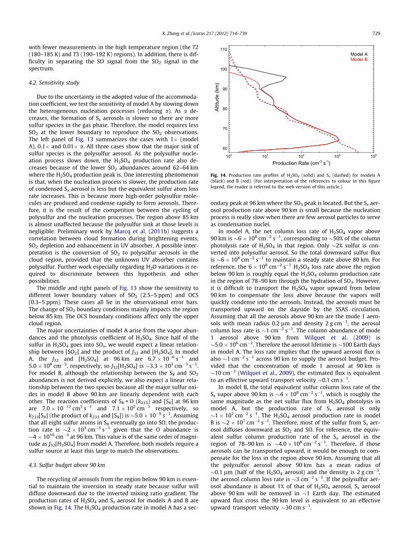
The recycling of aerosols from the region below 90 km is essen-tial to maintain the inversion in steady state because sulfur willdiffuse downward due to the inverted mixing ratio gradient. Theproduction rates of H2SO4 and Sx aerosol for models A and B areshown in Fig. 14. The H2SO4 production rate in model A has a sec-

ondary peak at 96 km where the SO3 peak is located. But the Sx aer-osol production rate above 90 km is small because the nucleationprocess is really slow when there are few aerosol particles to serveas condensation nuclei.

In model A, the net column loss rate of H2SO4 vapor above90 km is �6 � 108 cm�2 s�1, corresponding to �50% of the columnphotolysis rate of H2SO4 in that region. Only �2% sulfur is con-verted into polysulfur aerosol. So the total downward sulfur fluxis �6 � 108 cm�2 s�1 to maintain a steady state above 80 km. Forreference, the 6 � 108 cm�2 s�1 H2SO4 loss rate above the regionbelow 90 km is roughly equal the H2SO4 column production ratein the region of 78–90 km through the hydration of SO3. However,it is difficult to transport the H2SO4 vapor upward from below90 km to compensate the loss above because the vapors willquickly condense into the aerosols. Instead, the aerosols must betransported upward on the dayside by the SSAS circulation.Assuming that all the aerosols above 90 km are the mode 1 aero-sols with mean radius 0.2 lm and density 2 g cm�3, the aerosolcolumn loss rate is �1 cm�2 s�1. The column abundance of mode1 aerosol above 90 km from Wilquet et al. (2009) is�5.0 � 106 cm�2. Therefore the aerosol lifetime is �100 Earth daysin model A. The loss rate implies that the upward aerosol flux isalso �1 cm�2 s�1 across 90 km to supply the aerosol budget. Pro-vided that the concentration of mode 1 aerosol at 90 km is�10 cm�3 (Wilquet et al., 2009), the estimated flux is equivalentto an effective upward transport velocity �0.1 cm s�1.

In model B, the total equivalent sulfur column loss rate of theSx vapor above 90 km is �4 � 108 cm�2 s�1, which is roughly thesame magnitude as the net sulfur flux from H2SO4 photolysis inmodel A, but the production rate of Sx aerosol is only�1 � 107 cm�2 s�1. The H2SO4 aerosol production rate in modelB is �2 � 107 cm�2 s�1. Therefore, most of the sulfur from Sx aer-osol diffuses downward as SO2 and SO. For reference, the equiv-alent sulfur column production rate of the Sx aerosol in theregion of 78–90 km is �4.0 � 108 cm�2 s�1. Therefore, if thoseaerosols can be transported upward, it would be enough to com-pensate for the loss in the region above 90 km. Assuming that allthe polysulfur aerosol above 90 km has a mean radius of�0.1 lm (half of the H2SO4 aerosol) and the density is 2 g cm�3,the aerosol column loss rate is �3 cm�2 s�1. If the polysulfur aer-osol abundance is about 1% of that of H2SO4 aerosol, Sx aerosolabove 90 km will be removed in �1 Earth day. The estimatedupward flux cross the 90 km level is equivalent to an effectiveupward transport velocity �30 cm s�1.


If the SSAS circulation dominates the upper atmosphere, itmight be very efficient for transporting the aerosols upward. Thedownward velocity at 100 km near the anti-solar point is esti-mated to be �43 cm s�1 from the observed nighttime temperatureprofiles in Bertaux et al. (2007). Another derivation in Liang andYung (2009) obtained a different value of �1 cm s�1 at 100 km,which should be corrected to �10 cm s�1. So the two different cal-culations are consistent. However, one should always keep in mindthat the SSAS circulation is a longitudinal pattern, therefore thevertical velocity should strongly depend on the solar zenith angle.The SSAS pattern from recent VTGCM model results by Bougheret al. (personal communication) show that the vertical velocity inthe dayside is on the order of 10 cm s�1 above 100 km and onthe order of 1 cm s�1 from 80 to 100 km. Therefore the velocity re-quired in model A (�0.1 cm s�1) is readily achieved. But the veloc-ity implied by model B (�30 cm s�1) appears to be larger than thedynamic model results.

4.4. Timescales

The dynamics in the 1-D photochemistry-diffusion model isonly a simple parameterization for the complicated transition zonebetween 90 and 100 km. The aerosol microphysics is also simpli-fied because we just assume the instantaneous condensations ofH2O and H2SO4 and ignore the aerosol growth and loss processes.Future 2-D models including SSAS, zonal wind transport, micro-physical processes and photochemical processes for both the day-side and nightside hemisphere might be sufficient to represent allthe dynamical and chemical processes in the upper regions. Weestimate some typical timescales here.

(1) Transport: The timescale for the SSAS transport sSSAS is�104 s(based on Bertaux et al. (2007)) for vertical transport over the4 km scale height near 100 km. Zonal transport timescale dueto Retrograde Zonal (RZ) flow sRZ is�105 s for transport fromthe subsolar point to the antisolar point, provided that thethermal wind velocity is �50 m s�1 by Piccialli et al. (2008)based on the cyclostrophic approximation. Eddy diffusiontimescale seddy is also �105 s near 100 km (Fig. 15).

(2) Aerosol condensation: We assume that the condensation isdominated by the heterogeneous nucleation with timescalescond � 104–105 s (Fig. 15) for the accommodation coefficienta = 1. scond is inversely proportional to a in the free molecu-lar regime for the upper region. Therefore, the lower value ofa might be more appropriate for the H2SO4 condensation inmodel A since the mechanism assumes that the nighttimeH2SO4 vapor could be transported to the dayside andundergo photolysis. Homogeneous nucleation may beimportant in the dayside since both of H2SO4 and Sx arehighly supersaturated. For example, the dayside saturationratios at 100 km are about 106 and 104 for H2SO4 in modelA and S8 in model B, respectively. In model A, these daysidecondensation processes will compete with the photodissoci-ation of H2SO4. However, the homogeneous nucleation ratemarkedly depends on the SVP, which is a steep function oftemperature but not well determined in the lower tempera-ture range. Due to the condensation and photolysis of H2SO4

in the dayside, a zonal gradient of the H2SO4 vapor abun-dance from the nightside to the dayside would be expected.

(3) Chemistry: H2SO4 photolysis timescale sphoto depends on thecross section. For model A, sphoto is �105 s. Sx + O timescalesSxþO depends on the reaction coefficient and the atomicoxygen abundance, sSxþO is �1–10 s in the model B. That iswhy �0.1–1 ppt Sx could provide a sulfur source as largeas the photolysis of �0.1 ppm H2SO4 does. The reactionbetween polysulfur and atomic oxygen is so fast that it has

to happen in the nightside. However, as shown above,whether the circulation could support the Sx aerosol upwardflux across 90 km needs more future studies.

4.5. Basic differences between models A and B

Here, we present several basic differences between models Aand B for future considerations.

First, the two mechanisms are probably applied to different hor-izontal regions. By roughly estimating the chemical timescales anddynamical timescales, we found that the Sx + O reaction in model Bis much faster than the transport. As the Sx aerosols are evaporatedin the nightside, the Sx vapor will be oxidized in less than 10 s,therefore the SOx is first produced in the nightside and then trans-ported to the dayside by the zonal wind and photodissociated. Onthe other hand, H2SO4 photolysis has to happen in the dayside inmodel A. So the SOx should be first produced in the dayside andthen transported to the nightside. A big issue of model A is theH2SO4 condensation rate in the dayside since it is highly supersat-urated. If the homogeneous nucleation were very fast, the super-saturated vapor pressure could not be maintained, and theproduction of SO2 from the photolysis of H2SO4 would be too small.Therefore, the nightside H2SO4 abundances would be also super-saturated in order to supply enough H2SO4 for the dayside.

Secondly, the two mechanisms might require different aerosolflux from below. Since the aerosols cannot be fully recycled above90 km due to diffusion loss of sulfur, an upward aerosol flux isneeded. The estimated aerosol flux is �1 cm�2 s�1 and�3 cm�2 s�1, corresponding to an effective upward transportvelocity �0.1 cm s�1 and �30 cm s�1 for model A and model B,respectively. However, the estimation of Sx transport velocity hereis based on the assumption of the Sx/H2SO4 ratio �1% (Carlson,2010), which remains to be confirmed by future measurements.

Thirdly, in terms of possible observational evidence, model A re-quires H2SO4 number density �108 cm�3 around 96 km in the day-side, which might be observed. The estimated abundance of S8 inthe nightside is only �102 cm�3 around 96 km, which would behard to observe. SO3 might provide another possibility to distin-guish the two mechanisms because SO3 is controlled mainly bythe H2SO4 photolysis in model A but by the SO2 oxidization in mod-el B. The abundance of SO3 at 96 km is �3.3 � 107 cm�3 and�2.2 � 105 cm�3 for models A and B, respectively. Future observa-tions might be able to detect this difference. On the other hand, ifthe SO radical is produced mainly by the polysulfur oxidization inthe nightside, it might be possible to observe the nightglow of SOexcited states, in analogous to the O2 nightglow. The electronictransition of the SO (a1D ? X3R�) at 1.7 lm has been detected inIo’s atmosphere (de Pater et al., 2002).

4.6. OCS above the cloud tops

The OCS mixing ratio in the upper cloud layer is puzzling. OCSoriginates from the lower atmosphere. Marcq et al. (2005, 2006)reported an OCS mixing ratio �0.55 ± 0.15 ppm at �36 km,decreasing with altitude with a gradient of �0.28 ppm/km basedon the ground-based telescope IRTF observation. The VIRTIS mea-surement (Marcq et al., 2008) found the OCS mixing ratio rangingbetween 2.5 ± 1 and 4 ± 1 ppm at 33 km, agreeing with the previ-ous value �4.4 ppm from Pollack et al. (1993). Therefore, OCSwould only be �0.1 ppm or less in the lower cloud layer(�47 km). However, a sensitivity study of model A (Fig. 13) showsthat 0.3–5 ppm OCS at the upper cloud deck (�58 km) is requiredto reproduce the OCS mixing ratio at 65 km in the observed range0.3–9 ppb reported by Krasnopolsky (2010b). Krasnopolsky (2008)reported even larger values, �14 ppb around 65 km and �2 ppbaround 70 km. Venus Express results suggest that the upper limit

100 102 104 106 108

Timescale (s)

60

70

80

90

100

110

Altit

ude

(km

)

NuleationEddyS2 photolysisS3 photolysisS4 photolysis

Fig. 15. Timescales for the heterogeneous nucleation, eddy transport and photol-ysis for S2, S3 and S4.


of OCS is 1.6 ± 2 ppb in the region 70–90 km (Vandaele et al., 2008).But model A can produce only several tens of ppt OCS around70 km. One tentative detection of OCS reported from ground-basedobservations near 12 lm (Sonnabend et al., 2005) found an abun-dance consistent with that calculated by Mills (1998), which spec-ified 0.1 ppm OCS at 58 km. Besides, the scale height of OCS inmodel A is �1 km at 65 km, which matches only the lower limitof the observations (1–4 km from Krasnopolsky (2010b)). It seemsthat the eddy transport required in the upper cloud region needs tobe more efficient to transport OCS upward. This is also consistentwith the �4 km scale height of SO2 around 68 km in the Venus Ex-press measurements. Although the eddy diffusivity at �60 km hasbeen estimated to be less than 4.0 � 104 cm2 s�1 (Woo andIshimaru, 1981), it could have large variations in the cloud layer,leading to large variation in the detected OCS values and mayberelated to the decadal variation of SO2 at the upper cloud top(see Fig. 7 of Belyaev et al. (2008)).

The unexpected large amount of OCS will affect the polysulfurproduction. There are two pathways to produce atomic sulfur(see Fig. 9). One is the photodissociation of SO and ClS (Mills andAllen, 2007). The other way is from the photolysis of OCS. If theOCS abundance is large (e.g. model A), the primary source of atom-ic sulfur below �62 km is from the photolysis of OCS instead ofthat of SO and ClS. There are also two pathways to produce S2.One is from the chlorosulfane chemistry (Mills and Allen, 2007)and the other is from the reaction between S and OCS. It turnsout that the reaction rate of S + OCS in model A is as large as theClS2 photolysis below 60 km. Therefore if there is an abundantOCS layer near the lower boundary, it may greatly enhance the pro-duction of Sx in the 58–60 km region.

4.7. Elemental sulfur supersaturation

Even using the highest nucleation rate (a = 1), the model A re-sults show that the S2, S3, S4 and S5 are highly supersaturated basedon the SVP from Lyons (2008) (see Fig. 6). The column abundancesof gaseous S2, S3, S4 and S5 above 58 km are 1.4 � 1013 cm�2,9.0 � 1010 cm�2, and 2.1 � 1011 cm�2, 4.3 � 109 cm�2, respectively.S5 is supersaturated with the saturation ratio �1000 peaking at60 km but decreases rapidly. The saturation ratio of S4 is about107 at the lower boundary and becomes moderately supersatu-rated above 76 km. S3 is oversaturated by a factor of 105–1010 from58 to 100 km. S2 is extremely supersaturated at all altitudes. Thesaturation ratio is 108 at the bottom and the top, with a peak of1015 at 90 km, where the heterogeneous nucleation of S2 is negligi-ble compared with the production processes from atomic sulfurthrough the three-body reaction 2S + M, and the major loss pro-cesses of S2 are oxidization to SO and the photo-dissociation toatomic sulfur. As illustrated in Fig. 9, the main production pro-cesses of Sx can be summarized as S + Sx�1 ? Sx and S2 + Sx�2 ? Sx,but the reactions ClS + S2 and S2O + S2O are also important for S3

production at the bottom and top of the model atmosphere,respectively. The loss mechanisms of Sx include the heterogeneousnucleation, conversion to other allotropes, and oxidization throughSx + O ? Sx�1 + SO. Fig. 15 shows the comparison of the diurnallyaveraged photolysis timescales of S2, S3 and S4 with the timescalesof the nucleation and eddy transport. The S2 loss process is domi-nated by the nucleation from 58 km to about 72 km where thephotolysis is as fast as the nucleation, but the conversion from S2

to S4 is also important around 60 km. The photolysis timescalesof S3 and S4 are of the order of 1s, much smaller than the nucleationtimescale (�10 s at 60 km and �100 s at 70 km). Therefore, for S3

and S4, photolysis by visible light is the major loss pathway andthe heterogeneous nucleation processes are negligible. Since theS3 and S4 aerosols are the possible candidates of the unknownUV absorbers although they are unstable (Carlson, 2010), the con-

densed S3 and S4 are probably produced from the heterogeneous Sx

chemistry over the H2SO4 droplet surfaces (Lyons, 2008). Since thesupersaturation ratios are very large for Sx vapors, the homoge-neous nucleation process will be important and thus should beconsidered in future work. A proper treatment of the microphysicalprocesses coupled with atmosphere dynamical processes withinthe cloud layer is needed to elucidate the Sx chemistry.

4.8. Alternative hypotheses

Eddy diffusion is able to transport the species only from a re-gion of high mixing ratio to that of a low mixing ratio, and so itcannot generate an inversion layer. A sudden large injection ofSO2 from either volcano (Smrekar et al., 2010) or the instabilityin the cloud region (e.g., VMC measurements from Markiewiczet al. (2007)) may provide a sulfur source at �70 km, where thelong-term natural variability of SO2 has been documented butnot understood. However, it is difficult for these mechanisms to ex-plain the SO2 inversion layer above 80 km because: (1) Volcanoeruption could only reach 70 km but not higher based on a recentVenus convective plume model (Glaze et al., 2010); (2) Even if thesudden injection reaches �100 km high, it is also difficult to main-tain the steady SO2 inversion for an extended period in the VenusExpress era because the gas-phase SO2 lifetime is short (�a fewEarth days or less above 70 km). A continuous upwelling of SO2

from the lower region to the upper region (advection) is possiblealthough the dynamics maintaining the inversion profiles is notunderstood. The upward flux can be estimated by balancing thedownward flux by diffusion:

U ¼ Kzz½M�dfdz

ð8Þ

where U is the vertical flux, Kzz eddy diffusivity, [M] number den-sity, f mixing ratio, and z altitude. Assuming the Kzz � 106 cm2 s�1,df � 10�7, [M] � 1017 cm�3 (at 80 km), dz � 10 km (80–90 km), weobtain U � 1010 cm�2 s�1. To maintain the inversion requires anequal upward flux at 80 km.

Compared with the dynamical mechanism which transportsSO2 directly from 80 km, our mechanism of in situ chemical pro-duction from parents transported in aerosol is more plausible be-cause: (1) the inversion can be explained by the shape of theequilibrium vapor pressure profile above 90 km (models A andB); (2) it needs the upward transport of aerosols only around the90 km region, where the SSAS circulation is strong and has beenverified by the nighttime warm layer (Bertaux et al., 2007).

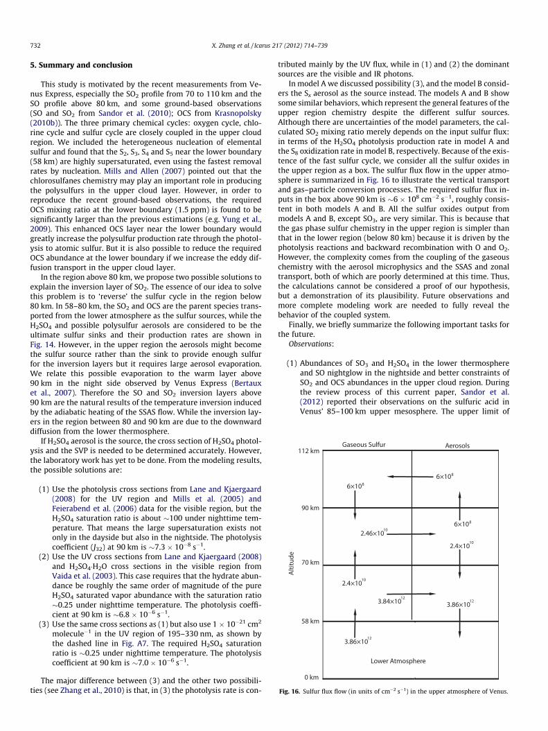
Fig. 16. Sulfur flux flow (in units of cm�2 s�1) in the upper atmosphere of Venus.


5. Summary and conclusion

This study is motivated by the recent measurements from Ve-nus Express, especially the SO2 profile from 70 to 110 km and theSO profile above 80 km, and some ground-based observations(SO and SO2 from Sandor et al. (2010); OCS from Krasnopolsky(2010b)). The three primary chemical cycles: oxygen cycle, chlo-rine cycle and sulfur cycle are closely coupled in the upper cloudregion. We included the heterogeneous nucleation of elementalsulfur and found that the S2, S3, S4 and S5 near the lower boundary(58 km) are highly supersaturated, even using the fastest removalrates by nucleation. Mills and Allen (2007) pointed out that thechlorosulfanes chemistry may play an important role in producingthe polysulfurs in the upper cloud layer. However, in order toreproduce the recent ground-based observations, the requiredOCS mixing ratio at the lower boundary (1.5 ppm) is found to besignificantly larger than the previous estimations (e.g. Yung et al.,2009). This enhanced OCS layer near the lower boundary wouldgreatly increase the polysulfur production rate through the photol-ysis to atomic sulfur. But it is also possible to reduce the requiredOCS abundance at the lower boundary if we increase the eddy dif-fusion transport in the upper cloud layer.

In the region above 80 km, we propose two possible solutions toexplain the inversion layer of SO2. The essence of our idea to solvethis problem is to ‘reverse’ the sulfur cycle in the region below80 km. In 58–80 km, the SO2 and OCS are the parent species trans-ported from the lower atmosphere as the sulfur sources, while theH2SO4 and possible polysulfur aerosols are considered to be theultimate sulfur sinks and their production rates are shown inFig. 14. However, in the upper region the aerosols might becomethe sulfur source rather than the sink to provide enough sulfurfor the inversion layers but it requires large aerosol evaporation.We relate this possible evaporation to the warm layer above90 km in the night side observed by Venus Express (Bertauxet al., 2007). Therefore the SO and SO2 inversion layers above90 km are the natural results of the temperature inversion inducedby the adiabatic heating of the SSAS flow. While the inversion lay-ers in the region between 80 and 90 km are due to the downwarddiffusion from the lower thermosphere.

If H2SO4 aerosol is the source, the cross section of H2SO4 photol-ysis and the SVP is needed to be determined accurately. However,the laboratory work has yet to be done. From the modeling results,the possible solutions are:

(1) Use the photolysis cross sections from Lane and Kjaergaard(2008) for the UV region and Mills et al. (2005) andFeierabend et al. (2006) data for the visible region, but theH2SO4 saturation ratio is about �100 under nighttime tem-perature. That means the large supersaturation exists notonly in the dayside but also in the nightside. The photolysiscoefficient (J32) at 90 km is �7.3 � 10�8 s�1.

(2) Use the UV cross sections from Lane and Kjaergaard (2008)and H2SO4�H2O cross sections in the visible region fromVaida et al. (2003). This case requires that the hydrate abun-dance be roughly the same order of magnitude of the pureH2SO4 saturated vapor abundance with the saturation ratio�0.25 under nighttime temperature. The photolysis coeffi-cient at 90 km is �6.8 � 10�6 s�1.

(3) Use the same cross sections as (1) but also use 1 � 10�21 cm2

molecule�1 in the UV region of 195–330 nm, as shown bythe dashed line in Fig. A7. The required H2SO4 saturationratio is �0.25 under nighttime temperature. The photolysiscoefficient at 90 km is �7.0 � 10�6 s�1.

The major difference between (3) and the other two possibili-ties (see Zhang et al., 2010) is that, in (3) the photolysis rate is con-

tributed mainly by the UV flux, while in (1) and (2) the dominantsources are the visible and IR photons.

In model A we discussed possibility (3), and the model B consid-ers the Sx aerosol as the source instead. The models A and B showsome similar behaviors, which represent the general features of theupper region chemistry despite the different sulfur sources.Although there are uncertainties of the model parameters, the cal-culated SO2 mixing ratio merely depends on the input sulfur flux:in terms of the H2SO4 photolysis production rate in model A andthe S8 oxidization rate in model B, respectively. Because of the exis-tence of the fast sulfur cycle, we consider all the sulfur oxides inthe upper region as a box. The sulfur flux flow in the upper atmo-sphere is summarized in Fig. 16 to illustrate the vertical transportand gas–particle conversion processes. The required sulfur flux in-puts in the box above 90 km is �6 � 108 cm�2 s�1, roughly consis-tent in both models A and B. All the sulfur oxides output frommodels A and B, except SO3, are very similar. This is because thatthe gas phase sulfur chemistry in the upper region is simpler thanthat in the lower region (below 80 km) because it is driven by thephotolysis reactions and backward recombination with O and O2.However, the complexity comes from the coupling of the gaseouschemistry with the aerosol microphysics and the SSAS and zonaltransport, both of which are poorly determined at this time. Thus,the calculations cannot be considered a proof of our hypothesis,but a demonstration of its plausibility. Future observations andmore complete modeling work are needed to fully reveal thebehavior of the coupled system.

Finally, we briefly summarize the following important tasks forthe future.

Observations:

(1) Abundances of SO3 and H2SO4 in the lower thermosphereand SO nightglow in the nightside and better constraints ofSO2 and OCS abundances in the upper cloud region. Duringthe review process of this current paper, Sandor et al.(2012) reported their observations on the sulfuric acid inVenus’ 85–100 km upper mesosphere. The upper limit of


H2SO4 mixing ratio is found to be 3 ppb (�106 cm�3), whichis two orders of magnitude less than the H2SO4 abundancerequired by Zhang et al. (2010).

Laboratory measurements:

(2) Measurements of photodissociation cross section of H2SO4 inthe UV region, especially in the lower energy range (�195–330 nm).

(3) Laboratory measurements of H2SO4 SVP in the lower tem-perature region (�150–240 K).

(4) Determination of polysulfur reaction coefficients.

Unsolved problems:

(5) An explanation of the longtime variation of SO2 at the uppercloud top �70 km and the possible variation of the OCSabundance in the upper cloud region.

(6) The microphysical properties of Sx and H2SO4 aerosols, theirformation and loss processes, transport, vertical profiles andthe cause of the multi-modal distributions.

(7) Coupled mesosphere-thermosphere (�58–135 km) chemis-try including the neutral species and ions to reveal the roleof SSAS transport in both dayside and nightside of Venus.

Acknowledgments

We thank E. Marcq for sharing his latest work with us and forhelpful discussions, C. Parkinson, S. Bougher and A. Brecht for pro-viding us the recent VTGCM results, A. Ingersoll and D. Yang forinsightful comments, R. Zeng for checking the chemical reaction ta-ble, M. Gerstell, M. Line and other members of Yung’s group at Cal-tech for reading the manuscript. We are indebted to T. Clancy forpointing out the importance of Sx aerosols as a potential sourceof SO2 in the mesosphere of Venus. We acknowledge two anony-mous reviewers for their helpful comments. This research was sup-ported by NASA grant NNX07AI63G to the California Institute of

2000 3000 4000 5Wavele

2.02.22.42.62.83.03.2

Qex

t

2000 3000 4000 5Wavele

0.65

0.70

0.75

0.80

Asym

met

ry F

acto

r

2000 3000 4000 5Wavele

0.85

0.90

0.95

1.00

SSA

Fig. A1. Optical properties of mode 1 (solid) and mode 2 (dashed) aerosols above the mextinction efficiency; Middle panel: asymmetry factor; Lower panel: single scattering albe

Technology. M. C. Liang was funded by NSC Grant 98-2111-M-001-014-MY3 to Academia Sinica. F.P. Mills was supported bygrants under the Australian Research Council Discovery Projectsand Linkage International schemes. D. A. Belyaev acknowledgessupport from CNES for a post-doc position at LATMOS.

Appendix A

A.1. Radiative transfer

The diurnally averaged radiation calculation here is modified onthe basis of Mills (1998). The direct attenuated flux and Rayleighscattering calculations remain the same (see details in the Appen-dix H, and I of Mills (1998)). In this study we adopt 550 log-linearoptical depth grids, 112 wavelengths from 960 to 8000 Å, 14 zenithangles for the incoming photons, 8 Gaussian angles for the diffusedphotons. The wavelength-independent middle cloud albedo at thelower boundary is assumed to be 0.6. The depolarization factor ofCO2 Rayleigh scattering equals 0.443.

The absorption of the unknown UV absorber and scattering pro-cesses of haze and cloud particles are crucial for the radiation field,especially in the upper cloud layer. We follow the procedure de-scribed in Crisp (1986). First, we calculated the optical depths fromthe bimodal aerosol profiles (see Appendix B) and scaled to matchthe optical depth values in Table 2 (equatorial cloud model) ofCrisp (1986). Aerosol optical properties are calculated using Mie-code based on the parameters of equator hazes in Table 1 of Crisp(1986). For mode 1, the refractive index is 1.45, radius0.49 ± 0.22 lm. For mode 2, the refractive index is 1.44, radius1.18 ± 0.07 lm. Fig. A1 shows the scattering efficiencies (upper pa-nel) and asymmetry factors (middle panel) of the two modes. Sincethe asymmetry factors do not vary with wavelength significantly,we choose 0.74 as the mean value for all wavelengths. The UV ab-sorber is introduced by decreasing the single scattering albedo ofthe mode 1 aerosol between 3100 and 7800 Å. We take the empir-ical absorption efficiency values from Table 4 of Crisp (1986).Fig. A1 (lower panel) shows the single scattering albedo of themode 1 aerosol mixed with the UV absorber. Because the single

000 6000 7000 8000ngth (Å)

000 6000 7000 8000ngth (Å)

000 6000 7000 8000ngth (Å)

iddle cloud top (�58 km) based on the parameters from Crisp (1986). Upper panel:do mixed with the empirical albedo of the unknown UV absorber from Crisp (1986).


scattering albedo is not constant (from 0.85 to 1) with wavelength,we use the wavelength-dependent values in the calculation. Thespectral actinic fluxes (in units of photons cm�2 s�1 Å�1) for 58,70 and 112 km at 45�N are plotted as functions of wavelength inFig. A2, although in this study our calculation is at 70�N only.Due to absorptions by CO2, SO2 and SO, the UV flux decreases rap-idly as it penetrates deeper into the atmosphere. Rayleigh scatter-ing and aerosol scattering result in the larger actinic flux in thecloud and haze layers than that at the top of the atmosphere. Inthe wavelength range large than 2000 Å, the actinic flux peaksaround �65 km. The UV actinic flux at the lower boundary(�58 km) between 2000 and 3000 Å is roughly anti-correlatedwith the SO2 cross sections and the minimum in its the cross sec-tion profile near 2400 Å may open a window for the UV flux to pen-etrate to the lower atmosphere of Venus. There is an analogousspectral window in the terrestrial atmosphere between 200 and220 nm (Froidevaux and Yung, 1982).

1000 2000 3000 4000 5000 6000 7000Wavelength (Å)

106

108

1010

1012

1014

Spec

tral A

ctin

ic F

lux

(Pho

tons

cm

−2 s

−1Å−1

)

58km70km112km

Fig. A2. Spectral actinic flux in the middle atmosphere of Venus at 45�N.

0.1 1.0 10.0 100.0 1000.0Concentration (cm-3)

60

70

80

90

100

110

Altit

ude

(km

)

10-10 10-9 10-8 10-7 10-6 10-5

Equivalent Sulfur Mixing Ratio

60

70

80

90

100

110

Altit

ude

(km

)

Fig. A3. Left panel: concentration profiles of mode 1 (solid) and mode 2 (dashed)aerosols based on the upper haze profiles from Wilquet et al. (2009) above 72 kmand upper cloud particle profiles from Knollenberg and Hunten (1980) from 58 to65 km. Data are not available in the red region (�66–70 km). Right panel: theequivalent sulfur mixing ratio (ESMR) by volume computed from the H2SO4 aerosol(solid line) and the polysulfur aerosol (dashed line). See the text for details. (Forinterpretation of the references to colour in this figure legend, the reader is referredto the web version of this article.)

Appendix B

B.1. Nucleation rate of elemental sulfur

B.1.1. Aerosol profileAbove the middle cloud top (�58 km), the aerosols are found to

exhibit a bimodal distribution in the upper cloud layer (58–70 km)and upper haze layer (70–90 km). In this study we combine theupper haze profiles from Wilquet et al. (2009) above 72 km andupper cloud particle profiles from Knollenberg and Hunten(1980) from 58 to 65 km. Due to the lack of data for the interme-diate altitudes (65–72 km) at present, interpolation is applied.Fig. A3 shows the bimodal aerosol profiles (left panel).

From the aerosol abundances, we can estimate the sulfur con-tent. Mode 1 aerosols are �0.2 lm in radius constantly for all alti-tudes. For mode 2 aerosols, we use 0.7 lm above 72 km (Wilquetet al., 2009) for the haze particles and 1.1 lm below for the cloudparticles (Knollenberg and Hunten, 1980). The right panel in Fig. A3shows the equivalent sulfur mixing ratio (ESMR) by volume com-puted from the H2SO4 aerosol (solid line) abundances by assumingthat the H2SO4 aerosol density is 2 g cm�3 and weight percent are85% and 75% below and above 72 km, respectively. The ESMR in theH2SO4 droplet is close to 1 ppm at all altitudes, which is enough forthe enhancement of sulfur oxides above 80 km. By assuming thatthe radius of elemental sulfur is about half of the H2SO4 aerosol ra-dius and the density is also 2 g cm�3, we found the ESMR in ele-mental sulfurs in excess of 1 ppb level at most altitude (Fig. A3,right panel, dashed line).

B.1.2. Heterogeneous nucleationThe nucleation rate of elemental sulfurs onto H2SO4 droplets is

estimated as follows. The nucleation rate constant in the contin-uum regime (where the particle size is much larger than the vapormean free path k) is expressed as (Seinfeld and Pandis, 2006):Jc = 4pRpDs, where Rp is the H2SO4 aerosol radius and Ds the molec-ular diffusivity of elemental sulfur vapor.

However, in the Venus cloud layer, the Knudsen Number Kn (=k/Rp) of Sx vapor is not far from 1, so the nucleation process lies in thetransition regime where the mean free path k of the diffusing vapormolecule (e.g., Sx vapor) is comparable to the pre-existing aerosolsize. Therefore, we adopt the Dahneke approach (Dahneke, 1983),which matches the fluxes of continuum regime (K� 1) and freemolecular regime (Kn � 1) by introducing a function f(Kn):

f ðKnÞ ¼1þ Kn

1þ 2Knð1þ KnÞ=aðA1Þ

where a is the molecular accommodation coefficient, which is theprobability of sticking when the vapor molecule encounters a parti-cle. Here the mean free path k in Kn is defined as 2Ds/v, where v isthe mean thermal velocity of the vapor molecule.

Finally we obtain the nucleation rate constant:

J ¼ f ðKnÞJc ¼4pRpDsð1þ KnÞ

1þ 2Knð1þ KnÞ=aðA2Þ

The molecular diffusivity Ds of sulfur vapor can be estimatedusing hard sphere approximation: Ds = b/N, where N is the totalCO2 gas density in the environment and b is the binary collisionparameter:

B ¼ 3

4pðds þ dgÞ22pkTðms þmgÞ

msmg

� �1=2

ðA3Þ

where ds and dg are the diameters of Sx and CO2 molecule, respec-tively (assuming ds = dg = 3 Å), k is the Boltzmann constant, T isthe temperature, ms and mg are the mass of Sx and CO2 molecule,respectively. Fig. 15 shows the total nucleation timescale of S2


calculated from two modes of aerosols (roughly the same for otherallotropes), together with the eddy transport timescale andphotolysis timescales of S2, S3 and S4. See the discussion inSection 4.

Appendix C

C.1. H2SO4 and Sx vapor abundances

C.1.1. H2SO4

If sulfuric acid is in thermodynamic equilibrium with the sur-rounding atmosphere, the saturation vapor pressure (SVP) overH2SO4 aerosol should mainly depend on the temperature and aer-osol composition. However, non-thermodynamic equilibrium inthe real atmosphere is common because the chemical and dynamicprocesses, such as the chemical production, loss, condensation,evaporation and transport, are often involved and play importantroles. The condensation efficiency, which depends on many micro-physical properties of the system like the temperature, diffusivity,aerosol size, surface tension, and interaction between moleculesand aerosols, will greatly affect the H2SO4 vapor pressure overthe liquid droplets. The very low condensation rate could causelarge supersaturation of the H2SO4 vapor. For example, the satura-tion ratio of H2SO4 in the lower stratospheric sulfate layer (Jungelayer) on Earth has been observed to be as large as 102–103

(Arnold, 2006). A similar situation may exist in the Venus upperhaze layer on the dayside when the H2SO4 vapor on the night sideis transported to the dayside, because the SVP of H2SO4 in the nightside is several orders of magnitude larger than that in the dayside(Zhang et al., 2010) due to the large temperature difference above90 km. Zhang et al. (2010) proposed that this might be the keymechanism to explain the SO2 inversion layer because the night-time H2SO4 abundance could be enough to produce the observedSO2 under photochemical processes if the H2SO4 photolysis crosssection is 100 time larger than the current data from Vaida et al.(2003).

10-8 10-6 10-4 10-2 100

Water Activity

60

70

80

90

100

110

Altit

ude

(km

)

10-7 10H2O Mix

60

70

80

90

100

110

Night

%07

06

%88

Day

88%

Fig. A4. Left panel: water activity profiles based on the daytime and nighttime temperawhich H2SO4 weight percent for each altitude could be inferred by comparing the observtemperature situations, respectively.

In the condensation processes, we assume that the sulfate aer-osol will quickly establish equilibrium with respect to water be-cause there are more collisions of aerosol particles with H2Omolecules than with H2SO4 molecules. Therefore, we could derivethe H2SO4 aerosol composition (weight percent) from the wateractivity (or equilibrium relative humidity) defined as the partialpressure of water vapor divided by the SVP over pure water underthe same temperature. The water activity is shown in Fig. A4 (leftpanel) for day and night temperature profile, respectively. We usedthe H2O SVP as function of temperature from Tabazadeh et al.(1997), which is valid between 185 and 260 K.

PH2O¼exp 18:4524�3:5052�103

T�3:3:92�105

T2 �1:2725�107

T3

!

ðA4Þ

where PH2O is the SVP of H2O in mbar and T is temperature. Weextrapolated the formula to the entire temperature range (156–274 K) of Venus mesosphere so there would be some uncertaintiesabove 84 km for the dayside temperature and in the 84–90 km forthe nightside.

The H2SO4 weight percent is roughly estimated by comparingthe observed H2O mixing ratio profile with the theoretical profilesunder different H2SO4 compositions, as shown in Fig. A4 (the mid-dle and right panels). For the 50–80 wt.% H2SO4, we computed theH2O mixing ratio profiles based on Clegg and Brimblecombe (1995)and Tabazadeh et al. (1997). For the more concentrated acids, ourcalculation is based on Gmitro and Vermeulen (1964) although itmay not be very accurate for the low temperature (Mills, 1998).There are also some uncertainties in applying the Tabazadehet al. (1997) formula to Venus because the Clegg andBrimblecombe (1995) is only valid if the water activity larger than0.01. The atmosphere of Venus is very dry (Fig. A4), and so actuallyonly the results in the region from 85 to 100 km in the dayside and85–90 km in the nightside seem robust. However, as we showedbefore, the H2O SVP may have some uncertainties in those regions.Therefore, the H2SO4 weight percent derived here is only a roughestimate based on the current knowledge.

-6 10-5

ing Ratio10-7 10-6 10-5

H2O Mixing Ratio

60

70

80

90

100

110

%05

%08

%

%48 %48

%88

%69

%08

%07%06 %05

%07

%08 %48%88

%09

%08 %08

%08

ture profiles. Middle and right panels: equilibrium H2O mixing ratio contours fromed H2O profile (dashed line). The middle and right panels are for the day and night


The H2SO4 weight percent falls with altitude, associated withthe increase of relative humidity due to the temperature decrease.The values are about 90–84% in 58–70 km and 84–60% in 70–90 km, which are roughly consistent with the H2SO4 compositionsobtained from aerosol refractive indexes based on the photometrymeasurements (85% and 75%, respectively). But in the region above90 km, the large contrast of dayside and nightside temperatures re-sults in large difference of the local H2SO4 weight percent. Forexample, H2SO4 at 100 km is �75% in the dayside but can be largerthan 96% in the nightside if the H2O vapor profiles are the same forboth hemispheres. Actually the temperature profile above 90 kmhas been found to be a function of longitude (Bertaux et al.,2007). Therefore, if the transport is efficient, the H2SO4 aerosolscould have a broad range distribution of various concentrationsabove 90 km but the H2SO4 vapor abundances might be mainlydetermined by the warmest nightside temperature since the vaporabundances is extremely sensitive to the temperature.

The H2SO4 SVP is another uncertainty and maybe the major one.In the supplementary material of Zhang et al. (2010), three H2SO4

SVP formulas as function of temperature and H2SO4 concentrationhave been discussed in details. These formulas could differ by sev-eral orders of magnitude but none of them has been verified in thetemperature range of upper atmosphere of Venus. Instead of usingthe H2SO4 weight percent profile derived in Fig. A4, we simply as-sumed 85% H2SO4 below 70 km and 75% from 70 to 90 km andused the vapor pressure formulas from Ayers et al. (1980) cor-rected by Kulmala and Laaksonen (1990):

ln P0H2SO4

¼ 16:259þ l� l0

8:3143Tþ 10156

� 1Tþ 0:38

Tc � T01þ ln

T0

T

� �� T0

T

� �� ðA5Þ

where Tc = 905 K, T0 = 360.15 K, P0H2SO4

is SVP of H2SO4 in atm, T is thetemperature, l and l0 are the chemical potentials of H2SO4 solu-tions of certain composition and pure acid, respectively. The valuesof l–l0 for the 85% and 75% H2SO4 are, respectively, 1555 cal�1

mole and 3681 cal�1 mole based on Giauque et al. (1960).In fact the H2SO4 abundances in the region below 80 km are not

important because the H2SO4 photolysis is negligible for the lower

10-25 10-20 10-15 10-10

H2SO4 Saturated Mixing Ratio

60

70

80

90

100

110

Altit

ude

(km

)

a

Fig. A5. Left panel: H2SO4 vapor volume mixing ratio profiles in equilibrium with the(H2SO4�H2O) vapor volume mixing ratio profiles.

region chemistry. But in the upper region the H2SO4 might behavelike a sulfur source rather than a sink, and large abundance ofH2SO4 is required in the upper region in order to reproduce theSO2 inversion layer (Zhang et al., 2010). So we adopted the formulaby Stull (1947) just for reference, simply because it gives the larg-est SVP in the Venus temperature range:

PH2SO4 ¼ 10�3954:90=Tþ9:4570 ðA6Þ

where PH2SO4 is the SVP of H2SO4 in mmHg and T is temperature. TheH2SO4 SVP profiles in Fig. A5 (left panel) show large difference be-tween the dayside and nightside caused by the difference in tem-peratures. Since H2SO4 is very hygroscopic, the right panel showsthe abundance of monohydrate (H2SO4�H2O), estimated based onthe extrapolation of the equilibrium constants from the Vaidaet al. (2003) for the Earth atmosphere (223–271 K in the literature).The abundances of H2SO4�H2O above 90 km are less than 5% andmuch less (<10�5) of that of pure H2SO4 for the dayside and night-side, respectively, although the equilibrium constants have not beenverified in the Venus temperature region (�160–240 K).

C.1.2. Sx

Lyons (2008) summarized the previous laboratory measure-ments and computed vapor pressure over the liquid sulfur allo-tropes and the total solid sulfur vapor pressures over theorthorhombic sulfur and the monoclinic sulfur below the meltingpoints. Based on the data, the author estimated the equilibrium va-por pressure over solid sulfur allotropes. In this study, we followthe same method and calculated the monoclinic Sx saturated vol-ume mixing ratio profiles under the daytime and nighttime tem-perature situations. The results are shown in Fig. A6.

Appendix D

D.1. Photolysis cross section

H2SO4 was thought to be photodissociated by the UV photonsonly. Burkholder et al. (2000) and Hintze et al. (2003) estimatedthe upper limits for the UV cross section of H2SO4 based on the fail-ure to detect any absorption beyond 140 nm. The upper limits are

10-24 10-22 10-20 10-18 10-16 10-14

SAM Saturated Mixing Ratio

60

70

80

90

100

110b

daytime (solid) and nighttime temperatures (dashed). Right panel: monohydrate

10-30 10-25 10-20 10-15 10-10

Saturated Mixing Ratio

60

70

80

90

100

110

Altit

ude

(km

)

S2

S3

S4 S5 S6S7

S8

Fig. A6. Saturated vapor volume mixing ratio profiles of Sx allotropes based on themonoclinic Sx saturated vapor pressure over solid Sx based on Lyons (2008), inequilibrium with the daytime (dashed) and nighttime (solid) temperatures.

1000 2000 3000 4000 5000 6000 7000 8000Wavelength (Å)

10−26

10−24

10−22

10−20

10−18

10−16

Cro

ss S

ectio

n (c

m2 m

olec

ule−1

)

Fig. A7. H2SO4 cross sections binned in the model grids. Solid: data from Lane andKjaergaard (2008) for the UV region, and Mills et al. (2005) and Feierabend et al.(2006) for the visible region. Dashed: same as the solid line but also with1 � 10�21 cm2 molecule�1 in the UV region of 195–330 nm.


assumed to be 1 � 10�21 cm2 molecule�1 in the interval 195–330 nm, 1 � 10�19 cm2 molecule�1 in 160–195 nm, and1 � 10�18 cm2 molecule�1 in 140–160 nm. Lane and Kjaergaard(2008) revisited the UV cross sections by calculating the electronictransitions based on the theoretical twin hierarchial approach andthey found that the cross section in the Lyman-a region(�121.6 nm) is about �6 � 10�17 cm2 molecule�1, much largerthan the previously assumed value. And it also seems that the crosssection in the interval 195–330 nm is much smaller than the upperlimits from Burkholder et al. (2000).

Vaida et al. (2003) proposed that in the visible region the exci-tation of the OH-stretching overtone transitions with v P 4(�38.6 kcal mole�1, or �742 nm) is also enough to photolyzeH2SO4 because the energy required for H2SO4 + ht ? SO3 + H2O isonly 32–40 kcal mole�1. This mechanism has been verified by thelaboratory experiments in 4v9 and 5v9 bands from the cavityring-down spectroscopy by Feierabend et al. (2006). Vaida et al.(2003) also proposed that, in the IR and visible regions the OH-stretching overtone transitions with v P 3 (�26.3 kcal/mol, or�1.09 lm) are able to generate the photodissociation of H2SO4�H2O

as well (required energy �25 kcal mole�1) and the total photolysiscoefficient is about �100 times larger than that of pure H2SO4,although a recent simulation by Miller and Gerber (2006) sug-gested that the H2SO4�H2O is more likely to thermally decomposeto H2SO4 and H2O before photodissociation.

The solid line in Fig. 2 shows the cross sections from Lane andKjaergaard (2008) for the UV region and Mills et al. (2005) andFeierabend et al. (2006) data for the visible region and binned inour model spectral grid. As shown in Table 1, the H2SO4 photolysiscoefficient is generally �10�7 s�1 in the upper atmosphere. It is�10�6 s�1 near the upper boundary (112 km) due to the photolysisby the Lyman-a line but only in a very thin layer (<1 km) becausethe Layman alpha intensity decreases very rapidly due to the CO2

absorption. The major contribution to the photolysis is the solarpumping of the vibrational overtones by the 740 nm red light(4v9 band, Vaida et al., 2003). The collisional deactivation mainlydepends on the atmospheric pressure. In Miller et al. (2007) thequantum yield is nearly unity above 60 km where the pressure is0.2 mbar in the Earth atmosphere. In Venus, this pressure level(0.2 mbar) is at �90 km which is the lower boundary of theH2SO4 photolysis region we are interested here. Therefore thequantum yield is assumed to be unity above 90 km.

However, Zhang et al. (2010) showed that the photolysis coeffi-cient �10�7 s�1 is not enough to produce the observed SO2, other-wise a very large supersaturation of H2SO4 (�100) under nighttimetemperature is needed. Although this supersaturation is possible(as seen in Earth), empirically they also found the required crosssection is about �100 times larger than that of pure H2SO4 if keep-ing the H2SO4 vapor abundances roughly the same as the nighttimesaturated abundances. This extreme situation may suggest theexistence of large amount of H2SO4�H2O and maybe other hydrates(like H2SO4�2H2O), although it seems not very likely not only be-cause the equilibrium abundance of the monohydrate is small(see Fig. A5) but also because the sulfuric acid hydrates might read-ily condense into the crystal phase even under the nighttime tem-perature (McGouldrick et al., 2010). Alternatively, the requiredlarge cross section actually could be achieved by assuming theUV cross section as the upper limit of 1 � 10�21 cm2 molecule�1

between 195 and 330 nm, as shown in dashed line in Fig. A7. Weconsider this possibility in the model A. Note that this change ofH2SO4 photolysis may not affect much for the Earth stratospherebelow 35 km because of the absorption of O3 Hartley band domi-nates the actinic flux in that region. However, this is very impor-tant for the Venus mesosphere above the cloud top since the SO2

absorption is not as strong as O3. The H2SO4 photolysis coefficientin this case is �8.3 � 10�6 s�1 at 90 km, roughly the same as that of�8.2 � 10�6 s�1 if we use the H2SO4�H2O photolysis cross sectioninstead (model B in Zhang et al. (2010)).

References

Arnold, F., 2006. Atmospheric aerosol and cloud condensation nuclei formation: Apossible influence of cosmic rays? Space Sci. Rev. 125, 169–186.

Atkinson, R., Baulch, D.L., Cox, R.A., Hampson Jr., R.F., Kerr, J.A., Troe, J., 1989.Evaluated kinetic and photochemical data for atmospheric chemistry:Supplement III. J. Phys. Chem. Ref. Data 18 (3), 881–1097.

Atkinson, R. et al., 2004. Evaluated kinetic and photochemical data for atmosphericchemistry: Volume I – Gas phase reactions of Ox, HOx, NOx and SOx species.Atmos. Chem. Phys. 4, 1461–1738.

Ayers, G.P., Gillett, R.W., Gras, J.L., 1980. On the vapor pressure of sulfuric acid.Geophys. Res. Lett. 7, 433–436.

Bahou, M., Chung, C.Y., Lee, Y.P., Cheng, B.M., Yung, Y.L., Lee, L.C., 2001. Absorptioncross sections of HCl and DCl at 135-232 nanometers: Implications forphotodissociation on Venus. Astrophys. J. Lett. 559, L179–L182.

Baulch, D.L., Duxbury, J., Grant, S.J., Montague, D.C., 1981. Evaluated kinetic data forhigh temperature reactions. Volume 4 homogeneous gas phase reactions ofhalogen- and cyanide-containing species. J. Phys. Chem. Ref. Data, 1–721.

Baulch, D.L. et al., 1992. Evaluated kinetic data for combustion modelling. J. Phys.Chem. Ref. Data 21, 411–734.


Belyaev, D. et al., 2008. First observations of SO2 above Venus’ clouds by means ofSolar Occultation in the Infrared. J. Geophys. Res. 113, E00B25. doi:10.1029/2008JE003143.

Belyaev, D., Montmessin, F., Bertaux, J.L., Mahieux, A., Fedorova, A., Korablev, O.,Marcq, E., Yung, Y.L., Zhang, X., 2012. Vertical profiling of SO2 and SO aboveVenus’ clouds by SPICAV/SOIR Solar Occultations. Icarus 217 (2), 740–751.

Bertaux, J.L. et al., 2007. A warm layer in Venus’ cryosphere and high-altitudemeasurements of HF, HCl, H2O and HDO. Nature 450, 646–649.

Brune, W.H., Schwab, J.J., Anderson, J.O., 1983. Laser magnetic resonance, resonancefluorescence, and resonance absorption studies of the reaction kinetics ofO + OH ? H+O2, O + HO2 ? OH + O2, N + OH ? H+NO, and N + HO2? productsat 300 K between 1 and 5 torr. J. Phys. Chem. A 87, 4503–4514.

Bryukov, M.G., Kachanov, A.A., Timonnen, R., Seetula, J., Vandoren, J., Sarkisova,O.M., 1993. Kinetics of HNO reactions with O2 and HNO. Chem. Phys. Lett. 208,392–398.

Burkholder, J.B., McKeen, S., 1997. UV absorption cross sections for SO3. Geophys.Res. Lett. 24, 3201–3204.

Burkholder, J.B., Mills, M., McKeen, S., 2000. Upper limit for the UV absorption crosssections of H2SO4. Geophys. Res. Lett. 27, 2493–2496.

Campbell, I.M., Thrush, B.A., 1967. The recombination of nitrogen atoms and thenitrogen afterglow. Proc. R. Soc. Lond. B. Biol. Sci. 296, 201–221.

Carlson, R.W., 2010. Venus’ Ultraviolet Absorber and Sulfuric Acid Droplets.International Venus Conference, Aussois, France, 4-4.

Chase, M.W., Davies, C.A., Downey, J.R., Frurip, D.J., McDonald, R.A., Syverud, A.N.,1985. JANAF thermochemical tables. Third edition. I, Al–Co. II, Cr–Zr. J. Phys.Chem. Ref. Data 14 (Suppl.), 1–1856.

Clancy, R.T., Sandor, B., Moriarty-Schieven, G., 2008. Venus upper atmospheric CO,temperature, and winds across the afternoon/evening terminator from June2007 JCMT sub-millimeter line observations. Planet. Space Sci. 56, 1344–1354.

Clegg, S.L., Brimblecombe, P., 1995. Application of a multicomponentthermodynamic model to activities and thermal properties of 0–40 mol kg�1

aqueous sulfuric acid from less than 200 K to 328 K. J. Chem. Eng. Data 40, 43–64.

Connes, P., Connes, J., Benedict, W.S., Kaplan, L.D., 1967. Traces of HCl and HF inatmosphere of Venus. Astrophys. J. 147, 1230–1237.

Crisp, D., 1986. Radiative forcing of the Venus mesosphere 1. Solar fluxes andheating rates. Icarus 67, 484–514.

Dahneke, B., 1983. Simple kinetic theory of Brownian diffusion in vapors andaerosols. In: Meyer, R.E. (Ed.), Theory of Dispersed Multiphase Flow. AcademicPress, New York, pp. 97–133.

de Pater, I., Roe, H., Graham, J.R., Strobel, D.F., Bernath, P., 2002. Detection of theforbidden SO a1D?X3R- rovibronic transition on Io at 1.7 lm. Icarus 156, 296–301.

DeMore, W.B. et al., 1994. Chemical Kinetics and Photochemical Data for Use inStratospheric Modeling: Evaluation Number 11.

DeMore, W.B. et al., 1997. Chemical Kinetics and Photochemical Data for Use inStratospheric Modeling: Evaluation Number 12.

Dodonov, A., Zelenov, V., Strunin, V., Talroze, V., 1981. Mass-spectrometricdetermination of rate constants of reaction steps 7. Flow-rate and contacttime in the mass-spectrometric probing of a diffusional cloud in a flow. Kinet.Catal. 22, 689–697.

Feierabend, K.J., Havey, D.K., Brown, S.S., Vaida, V., 2006. Experimental absoluteintensities of the 4v(9) and 5v(9) O–H stretching overtones of H2SO4. Chem.Phys. Lett. 420, 438–442.

Froidevaux, L., Yung, Y.L., 1982. Radiation and chemistry in the stratosphere:Sensitivity to O2 absorption cross sections in the Herzberg continuum. Geophys.Res. Lett. 9, 854–857.

Giauque, W.F., Hornung, E.W., Kunzler, J.E., Rubin, T.R., 1960. The thermodynamicproperties of aqueous sulfuric acid solutions and hydrates from 15-degrees K to300-degrees K. J. Am. Chem. Soc. 82, 62–70.

Glaze, L.S., Baloga, S.M., Wimert, J., 2010. Volcanic eruptions from linear vents onEarth, Venus and Mars: Comparisons with central vent eruptions. Lunar Planet.Sci. 41, 1147–1148 (abstract).

Gmitro, J.I., Vermeulen, T., 1964. Vapor–liquid equilibria for aqueous sulfuric acid.AIChE J. 10, 740–746.

Grillo, A., Reed, R., Slack, M.W., 1979. Infrared measurements of sulfur-dioxidethermal-decomposition rate in shock-waves. J. Chem. Phys. 70, 1634–1636.

He, Y., Liu, X., Lin, M.C., Melius, C.F., 1993. Thermal reaction of HNCO with NO2 atmoderate temperatures. Int. J. Chem. Kinet. 25, 845–863.

Hermans, C., Vandaele, A.C., Fally, S., 2009. Fourier transform measurements of SO2

absorption cross sections: I. Temperature dependence in the 24000–29000 cm�1 (345–420 nm) region. J. Quant. Spectrosc. Radiat. Transfer 110,756–765.

Hintze, P.E., Kjaergaard, H.G., Vaida, V., Burkholder, J.B., 2003. Vibrational andelectronic spectroscopy of sulfuric acid vapor. J. Phys. Chem. A 107, 1112–1118.

Knollenberg, R.G., Hunten, D.M., 1980. The microphysics of the clouds of Venus:Results of the Pioneer Venus particle size spectrometer experiment. J. Geophys.Res. 85, 8039–8058.

Krasnopolsky, V.A., 2006. A sensitive search for nitric oxide in the loweratmospheres of Venus and Mars: Detection on Venus and upper limit forMars. Icarus 182, 80–91.

Krasnopolsky, V.A., 2008. High-resolution spectroscopy of Venus: Detection of OCS,upper limit to H2S, and latitudinal variations of CO and HF in the upper cloudlayer. Icarus 197, 377–385.

Krasnopolsky, V.A., 2010a. Spatially-resolved high-resolution spectroscopy of Venus1. Variations of CO2, CO, HF, and HCl at the cloud tops. Icarus 208, 539–547.

Krasnopolsky, V.A., 2010b. Spatially-resolved high-resolution spectroscopy ofVenus 2. Variations of HDO, OCS, and SO2 at the cloud tops. Icarus 209, 314–322.

Krasnopolsky, V.A., 2010c. Venus night airglow: Ground-based detection of OH,observations of O2 emissions, and photochemical model. Icarus 207, 17–27.

Krasnopolsky, V.A., Pollack, J.B., 1994. H2O–H2SO4 system in Venus’ clouds and OCS,CO, and H2SO4 profiles in Venus’ troposphere. Icarus 109, 58–78.

Kulmala, M., Laaksonen, A., 1990. Binary nucleation of water-sulphuric acid system:comparison of classical theories with different H2SO4 saturation vapourpressures. J. Chem. Phys. 93, 696–701.

Lane, J.R., Kjaergaard, H.G., 2008. Calculated electronic transitions in sulfuric acidand implications for its photodissociation in the atmosphere. J. Phys. Chem. A112, 4958–4964.

Liang, M.C., Yung, Y.L., 2009. Modeling the distribution of H2O and HDO in the upperatmosphere of Venus. J. Geophys. Res. – Planets 114, E00B28.

Lindzen, R.S., 1981. Turbulence and stress owing to gravity-wave and tidalbreakdown. J. Geophys. Res. – Oceans Atmos. 86, 9707–9714.

Lovejoy, E.R., Hanson, D.R., Huey, L.G., 1996. Kinetics and products of the gas-phasereaction of SO3 with water. J. Phys. Chem. 100, 19911–19916.

Lu, C.W., Wu, Y.J., Lee, Y.P., Zhu, R.S., Lin, M.C., 2003. Experiments and calculationson rate coefficients for pyrolysis of SO2 and the reaction O + SO at hightemperatures. J. Phys. Chem. A 107, 11020–11029.

Lu, C.W., Wu, Y.J., Lee, Y.P., Zhu, R.S., Lin, M.C., 2006. Experimental and theoreticalinvestigation of rate coefficients of the reaction S (3P) + OCS in the temperaturerange of 298–985 K. J. Phys. Chem. 125, 164329. doi:10.1063/1.2357739.

Lyons, J.R., 2008. An estimate of the equilibrium speciation of sulfur vapor over solidsulfur and implications for planetary atmospheres. J. Sulfur Chem. 29, 269–279.

Marcq, E., Bezard, B., Encrenaz, T., Birlan, M., 2005. Latitudinal variations of CO andOCS in the lower atmosphere of Venus from near-infrared nightside spectro-imaging. Icarus 179, 375–386.

Marcq, E., Encrenaz, T., Bezard, B., Birlan, M., 2006. Remote sensing of Venus’ loweratmosphere from ground-based IR spectroscopy: Latitudinal and verticaldistribution of minor species. Planet. Space Sci. 54, 1360–1370.

Marcq, E., Bezard, B., Drossart, P., Piccioni, G., Reess, J.M., Henry, F., 2008. Alatitudinal survey of CO, OCS, H2O, and SO2 in the lower atmosphere of Venus:Spectroscopic studies using VIRTIS-H. J. Geophys. Res. – Planets 113, E00B07.doi:10.1029/2008JE003074.

Marcq, E., Belyaev, D., Montmessin, F., Fedorova, A., Bertaux, J.-L., Vandaele, A.C.,Neefs, E., 2011a. An investigation of the SO2 content of the venusianmesosphere using SPICAV-UV in nadir mode. Icarus 211, 58–69.

Marcq, E., Belyaev, D., Bertaux, J.-L., Fedorova, A., Montmessin, F., 2011b. Long-termmonitoring SO2 above the clouds of Venus using SPICAV-UV in nadir mode. EGUGeneral Assembly 13, EGU2011-2003.

Markiewicz, W.J. et al., 2007. Morphology and dynamics of the upper cloud layer ofVenus. Nature 450, 633–636.

McGouldrick, K., Toon, O.B., Grinspoon, D.H., 2010. Sulfuric acid aerosols in theatmospheres of the terrestrial planets. Planet. Space Sci. doi:10.1016/j.pss.2010.05.020.

Miller, Y., Gerber, R.B., 2006. Dynamics of vibrational overtone excitations of H2SO4,H2SO4-H2O: Hydrogen hopping and photodissociation processes. J. Am. Chem.Soc. 128, 9594–9595.

Miller, Y., Gerber, R.B., Vaida, V., 2007. Photodissociation yields for vibrationallyexcited states of sulfuric acid under atmospheric conditions. Geophys. Res. Lett.34, L16820. doi:10.1029/2007GL030529.

Mills, F.P., 1998. I. Observations and Photochemical Modeling of the Venus MiddleAtmosphere. II. Thermal Infrared Spectroscopy of Europa and Callisto. PhDThesis, California Institute of Technology, pp. 1–277.

Mills, F.P., Allen, M., 2007. A review of selected issues concerning the chemistry inVenus’ middle atmosphere. Planet. Space Sci. 55, 1729–1740.

Mills, M.J. et al., 2005. Photolysis of sulfuric acid vapor by visible light as a source ofthe polar stratospheric CN layer. J. Geophys. Res. 110, D08201. doi:10.1029/2004JD005519.

Mills, F.P., Esposito, L.W., Yung, Y.L., 2007. Atmospheric composition, chemistry, andclouds. In: Esposito, L.W., Stofan, E.R., Cravens, T.E. (Eds.), Exploring Venus as aTerrestrial Planet. American Geophysical Union, Washington, DC, pp. 73–100.

Moses, J.I., Bezard, B., Lellouch, E., Gladstone, G.R., Feuchtgruber, H., Allen, M., 2000.Photochemistry of Saturn’s atmosphere II. Effects of an influx of external oxygenI. Icarus 145, 166–202.

Moses, J.I., Zolotov, M.Y., Fegley, B., 2002. Photochemistry of a volcanically drivenatmosphere on Io: Sulfur and oxygen species from a Pele-type eruption. Icarus156, 76–106.

Pätzold, M. et al., 2007. The structure of Venus’ middle atmosphere and ionosphere.Nature 450, 657–660.

Pernice, H. et al., 2004. Laboratory evidence for a key intermediate in the Venusatmosphere: Peroxychloroformyl radical. Proc. Natl. Acad. Sci. 101, 14007–14010.

Piccialli, A. et al., 2008. Cyclostrophic winds from the Visible and Infrared ThermalImaging Spectrometer temperature sounding: A preliminary analysis. J.Geophys. Res. – Planets 113, E00B11. doi:10.1029/2008JE003127.

Pollack, J.B., Dalton, J.B., Grinspoon, D., Wattson, R.B., Freedman, R., Crisp, D., Allen,D.A., Bezard, B., Debergh, C., Giver, L.P., Ma, Q., Tipping, R., 1993. Near-infraredlight from Venus nightside – A spectroscopic analysis. Icarus 103, 1–42.

Prinn, R.G., 1975. Venus – Chemical and dynamical processes in stratosphere andmesosphere. J. Atmos. Sci. 32, 1237–1247.

Riley, P.S., Cosic, B., Fontijn, A., 2003. The H + NO recombination reaction over awide temperature range. Int. J. Chem. Kinet. 35, 374–380.

http://dx.doi.org/10.1029/2008JE003143

http://dx.doi.org/10.1029/2008JE003143

http://dx.doi.org/10.1063/1.2357739

http://dx.doi.org/10.1029/2008JE003074

http://dx.doi.org/10.1016/j.pss.2010.05.020

http://dx.doi.org/10.1016/j.pss.2010.05.020

http://dx.doi.org/10.1029/2007GL030529

http://dx.doi.org/10.1029/2004JD005519

http://dx.doi.org/10.1029/2004JD005519

http://dx.doi.org/10.1029/2008JE003127


Sander, S.P. et al., 2002. Chemical Kinetics and Photochemical Data for Use inAtmospheric Studies: Evaluation Number 14. Jet Propulsion Laboratory,California Institute of Technology, Pasadena, CA.

Sander, S.P. et al., 2006. Chemical Kinetics and Photochemical Data for Use inAtmospheric Studies: Evaluation Number 15. Jet Propulsion Laboratory,California Institute of Technology, Pasadena, CA.

Sandor, B.J., Clancy, R.T., Moriarty-Schieven, G., Mills, F.P., 2010. Sulfur chemistry inthe Venus mesosphere from SO2 and SO microwave spectra. Icarus 208, 49–60.

Sandor, B.J., Clancy, R.T., Moriarty-Schieven, G.H., 2012. Upper limits for H2SO4 inthe mesosphere of Venus. Icarus 217 (2), 839–844.

Seiff, A., 1983. Models of Venus’s atmospheric structure. In: Hunten, D.M., Colin, L.,Donahue, T.M., Moroz, V.I. (Eds.), Venus. University of Arizona Press, Tucson,Arizona, pp. 1045–1048.

Seinfeld, J.H., Pandis, S.N., 2006. Atmospheric Chemistry and Physics: From AirPollution to Climate Change. John Wiley & Sons, Inc., New York.

Singleton, D.L., Cvetanovic, R.J., 1988. Evaluated chemical kinetic data for thereactions of atomic oxygen O(3P) with sulfur-containing-compounds. J. Phys.Chem. Ref. Data 17, 1377–1437.

Smrekar, S.E. et al., 2010. Recent hot-spot volcanism on Venus from VIRTISemissivity data. Science 328, 605–608.

Sonnabend, G. et al., 2005. A new search for OCS in the middle atmosphere of Venus.Bull. Am. Astron. Soc. 37, 750.

Stull, D.R., 1947. Vapor pressure of pure substances—Inorganic compounds. Ind.Eng. Chem. 39, 540–550.

Sun, F. et al., 2001. Reactions of NH2 with NO2 and of OH with NH2O. J. Phys. Chem.A 105, 6121–6128.

Sundaram, M.S., Mills, F.P., Allen, M., Yung, Y.L., 2011. An initial model assessmentof NOx photochemistry on Venus with heterogeneous oxidation of CO. In:Proceedings of the 10th Australian Space Science Conference, Brisbane,Australia, 119–132.

Tabazadeh, A., Toon, O.B., Clegg, S.L., Hamill, P., 1997. A new parameterization ofH2SO4/H2O aerosol composition: Atmospheric implications. Geophys. Res. Lett.24, 1931–1934.

Vaida, V., Kjaergaard, H.G., Hintze, P.E., Donaldson, D.J., 2003. Photolysis of sulfuricacid vapor by visible solar radiation. Science 299, 1566–1568.

Vandaele, A.C. et al., 2008. Composition of the Venus mesosphere measured by SolarOccultation at Infrared on board Venus Express. J. Geophys. Res. 113, E00B23.doi:10.1029/2008JE003140.

Vandaele, A.C., Hermans, C., Fally, S., 2009. Fourier transform measurements of SO2

absorption cross sections: II. Temperature dependence in the 29000–44000 cm�1 (227–345 nm) region. J. Quant. Spectrosc. Radiat. Transfer 110,2115–2126.

Von Zahn, U., Krankowsky, D., Mauersberger, K., Nier, A.O., Hunten, D.M., 1980.Venus thermosphere – In situ composition measurements, the temperatureprofile, and the homopause altitude. Science 203, 768–770.

Wilquet, V. et al., 2009. Preliminary characterization of the upper haze by SPICAV/SOIR Solar Occultation in UV to mid-IR onboard Venus Express. J. Geophys. Res.114, E00B42. doi:10.1029/2008JE003186.

Woo, R., Ishimaru, A., 1981. Eddy diffusion-coefficient for the atmosphere of Venusfrom radio scintillation measurements. Nature 289, 383–384.

Yung, Y.L., DeMore, W.B., 1982. Photochemistry of the stratosphere of Venus:Implications for atmospheric evolution. Icarus 51, 199–247.

Yung, Y.L. et al., 2009. Evidence for carbonyl sulfide (OCS) conversion to CO in thelower atmosphere of Venus. J. Geophys. Res. 114, E00B34. doi:10.1029/2008JE003094.

Zhang, X., Liang, M.C., Montmessin, F., Bertaux, J.L., Parkinson, C., Yung, Y.L., 2010.Photolysis of sulphuric acid as the source of sulphur oxides in the mesosphereof Venus. Nat. Geosci. 3, 834–837.

http://dx.doi.org/10.1029/2008JE003140

http://dx.doi.org/10.1029/2008JE003186

http://dx.doi.org/10.1029/2008JE003094

http://dx.doi.org/10.1029/2008JE003094

sulfur chemistry in the middle atmosphere of venussulfur chemistry in the middle atmosphere of venus...

Documents