sulfate and alkali silica resistance sudheen anantharaman

SULFATE AND ALKALI SILICA RESISTANCE

OF CLASS C & F FLY ASH REPLACED BLENDED CEMENTS

by

Sudheen Anantharaman

A Thesis Presented in Partial Fulfillment

of the Requirements for the Degree

Master of Science

ARIZONA STATE UNIVERSITY

May 2008

SULFATE RESISTANCE AND ALKALI SILICA RESISTANCE

OF CLASS C & F REPLACED BLENDED CEMENTS

by

Sudheen Anantharaman

has been approved

December 2007

Graduate Supervisory Committee:

Barzin Mobasher, Chair

Apostolos Fafitis

Claudia Zapata

APPROVED BY THE GRADUATE COLLEGE

iii

ABSTRACT

Methodologies to reduce the dependence on Portland cement in concrete

production are desirable from a sustainability perspective since Portland cement

production is a major contributor to the greenhouse gas emission. The use of fly ash as a

cement replacement makes the concrete less permeable to harmful ions due to its finer

particle size distribution and pozzolanic reactions. This results in an enhanced high

performance and more durable concrete.

The concrete industry faces questions involving the characteristics of fly ash that

can be tolerated for the performance-based specification. The current trends are limited to

the production of Type IP cements containing 20% Class F fly ash. Two main

degradation mechanisms of sulfate attack (SA) and alkali silica reaction (ASR) are

addressed in this study. The effect of fly ash in changing the sulfate attack and Alkali-

Silica resistance of concrete for a range of replacement (10-40 %) of Class F and Class C

fly ashes was determined using both experimental and theoretical modeling.

A series of durability tests on the proposed mixes were conducted and guidelines

were developed for concrete containing high doses of Class C and F fly ash. The model

used for the prediction of sulfate resistance of blended cement samples was developed by

Tixier and Mobasher. A simplified version of this model based on diffusion reaction

assumption with a series solution was used. Diffusivity measures were obtained by

applying the model to the expansion time-history data. Results show that both Class C

and F fly ash replacements enhanced the resistance of mortars and pastes specimen to

both sulfate attack and alkali silica reaction. It was also observed that Class C fly ash

needs to be used in higher replacement levels to achieve satisfactory results.

iv

The study of different specimen sizes showed that smaller specimens could be used to

understand the mechanism of degradation in a much shorter duration of time, while

modeling techniques helped in understanding the diffusion and elastic modulus behavior

with the addition of fly ash.

v

TABLE OF CONTENTS

Page

LIST OF TABLES............................................................................................................ IX

LIST OF FIGURES ............................................................................................................X

NOMENCLATURE ...................................................................................................... XIV

DEDICATION.................................................................................................................XV

ACKNOWLEDGMENTS ............................................................................................. XVI

CHAPTER

1. INTRODUCTION ...........................................................................................................1

1.1. Overview...........................................................................................................1

1.2. Problem Statement ............................................................................................2

1.3. Objective of the Study ......................................................................................2

1.4. Scope of the Study ............................................................................................3

1.5. Organization of Report .....................................................................................4

2. LITERATURE REVIEW ................................................................................................6

2.1. Fly Ash and its Engineering Properties ............................................................6

2.2. Pozzolanic Reaction........................................................................................12

2.3. SEM and EDS.................................................................................................14

3. MATERIALS USED .....................................................................................................18

3.1. Cement ............................................................................................................18

3.2. Sand : Silica and Reactive...............................................................................19

3.3. Fly-Ash: Class C and Class F .........................................................................19

3.4. Microstructural Analysis of Material Used.....................................................21

vi

CHAPTER Page

4. EXPERIMENTAL PROCEDURE ................................................................................24

4.1. Introduction.....................................................................................................24

4.2. Sample Preparation .........................................................................................25

4.3. Solution Preparation for SA and ASR ............................................................28

4.4. Storage of Specimens in solution....................................................................29

4.5. Expansion Calculation ....................................................................................30

5. SULFATE ATTACK.....................................................................................................32

5.1. Introduction.....................................................................................................32

5.2. Literature review.............................................................................................33

5.2.1. Ettringite Formation........................................................................ 33

5.2.2. Factors Affecting Sulfate Attack .................................................... 37

5.3. Experimental Results and Observations .........................................................40

5.3.1. Cement Mortar Sample A (1” x 1” x11”) ....................................... 40

5.3.2. Cement Paste Sample A (1” x 1” x11”)........................................ 46

5.3.3. Cement paste Sample B (0.4” x 0.4” x 4”) .................................... 50

5.3.4. Compression Test Mortar .............................................................. 53

5.4. SEM and EDS analysis ...................................................................................60

5.5. Element Mapping Of Microstructure..............................................................64

6. ALKALI SILICA REACTION –ASR...........................................................................68

6.1. Introduction.....................................................................................................68

6.2. Literature Review............................................................................................70

6.2.1. Proposed Theories of ASR.............................................................. 70

vii

CHAPTER Page

6.2.2. Pessimum Effect and Aggregate Size Effect .................................. 71

6.2.3. Effect of SCM and Its Composition on ASR................................. 72

6.2.4. Effect of Cement composition on ASR .......................................... 73

6.3. Experimental Results ......................................................................................74

6.4. SEM and EDS Analysis ..................................................................................78

6.4.1. Microstructural Analysis for 7 Days of Exposure .......................... 78

6.4.2. Microstructural Analysis for 14 Days of Exposure ........................ 80

6.4.3. Microstructural Analysis for 28 Days of Exposure ........................ 82

6.4.4. Different Structures observed on the 28th

Day................................ 84

7. MODELING ..................................................................................................................86

7.1. Introduction.....................................................................................................86

7.2. Simplified Model ............................................................................................87

7.3. Parameters used for Modeling ........................................................................95

7.4. Results of Standard Size Mortar Specimen ....................................................96

7.5. Results of Standard Size Paste Specimen .....................................................100

7.6. Results of Modified Size Paste Specimen ....................................................102

8. CONCLUDING REMARKS.......................................................................................105

REFERENCES ................................................................................................................100

BIBLIOGRAPHY............................................................................................................108

APPENDIX

A - ABBREVIATIONS ...................................................................................................109

B - BATCHING OF SAMPLES......................................................................................112

viii

APPENDIX Page

C - CLEANING OF GRAPHS FROM RAW DATA .....................................................114

ix

LIST OF TABLES

Table Page

2.1.1 Specifications for fly ash in PCC. (ASTM C 618) - Class F and C......................... 11

3.1.1 Chemical analyses of cement used .......................................................................... 18

3.3.1 Chemical analyses of fly ash used ........................................................................... 20

4.1.1 Grading Requirements for Aggregates for ASR...................................................... 24

4.2.1 Total Number of Specimens Prepared ..................................................................... 27

5.3.4.1 Young’s Modulus for Class F Fly Ash ................................................................. 58

5.3.4.2 Strength Activity Index of Class F Fly Ash.......................................................... 58

5.3.4.3 Young’s Modulus for Class C Fly Ash................................................................. 59

5.3.4.4 Strength Activity Index of Class C Fly Ash ......................................................... 59

7.3.1 Parameters Considered For Paste Specimen............................................................ 95

7.3.2 Parameters Considered For Mortar Specimen ......................................................... 95

7.7.1 Surface area to Volume Ratio of Standard and Modified Sample......................... 104

8.1 Concluding Remarks for Standard mortar samples. ................................................. 105

B.1 Sample Excel Sheet for Batching............................................................................. 113

C.1 Excel Sheet for Raw Data. ....................................................................................... 115

x

LIST OF FIGURES

Figure Page

2.1.1 SEM for Fly ash and Cement..................................................................................... 7

2.1.2 Class C and F Fly ash............................................................................................... 11

2.3.1 Schematic drawing of a scanning electron microscope ........................................... 15

2.3.2 SEM Chamber where the samples are loaded.......................................................... 16

2.3.3 Sample SEM image taken at ASU........................................................................... 16

2.3.4 Sample EDS image taken at ASU............................................................................ 17

3.4.1 SEM & EDS for Cement Particles........................................................................... 21

3.4.2 SEM & EDS for Silica Sand Particles used in Sulfate Attack................................. 22

3.4.3 SEM & EDS for Reactive Sand Particles used in ASR........................................... 22

3.4.4 SEM & EDS for Class C Fly-Ash Particles............................................................. 23

3.4.5 SEM & EDS for Class F Fly-Ash Particles ............................................................. 23

4.2.1 A) Steel mold for ASTM C 1012 test (11”), B) Steel stud (end pin)

C) Steel stud held in the hardened specimen. .......................................................... 25

4.2.2 A) Plexy glass mold for modified test, B) Plexy glass stud (end pin) details,

C) Plexy glass stud attached to the specimen. ........................................................ 26

4.2.3. Mixing, Vibrating and Casting of Specimen. ......................................................... 27

4.3.1 Sodium Hydroxide ................................................................................................... 28

4.3.2 Sodium Sulfate......................................................................................................... 29

4.4.1 Sample A and Sample B Specimens in Sodium Sulfate solution ............................ 29

4.4.2 Specimens in Sodium hydroxide solution in Owen at 80°C.................................... 30

xi

4.5.1 A) Digital comparator with standard steel rod,

B) Digital comparator with Sample A and Sample B specimen.............................. 31

5.2.1.1 Ternary representation of ISA. ............................................................................. 35

5.2.1.2 Ternary representation of ESA. ............................................................................ 36

5.3.1.1 Average Expansions for Class C- Fly Ash (ESA) ................................................ 40

5.3.1.2 Average Expansions for Class F- Fly Ash (ESA)................................................. 41

5.3.1.3 Comparison Between 10 % (Class C , F ) & Control Specimen (ESA) ............... 43




5.3.1.7 Comparison Between Control Specimen (ESA) and Lime Water........................ 45











5.3.4.1 Compression Strength for Class C- Fly Ash (ESA) ............................................. 53

5.3.4.2 Compression Strength for Class F- Fly Ash (ESA).............................................. 54

xii

5.3.4.3 Comparison of Compressive Strength for Class F and Class C Fly Ash (ESA)

for the 1st Day........................................................................................................ 55


for the 28th

Day ..................................................................................................... 56


for the 126th

Day ................................................................................................... 56

5.4.1 SEM and EDS of Control Specimen on the 80th

Week (SA)................................... 60

5.4.2 SEM and EDS of Class F Specimen on the 80th

Week (SA)................................... 61

5.4.3 SEM and EDS of Class C Specimen on the 80th

Week (SA) .................................. 62

5.5.1 EDS mapping for Control Specimen on the 80th

Week (SA) .................................. 64

5.5.2 EDS mapping for Class C Specimen on the 80th

Week (SA) .................................. 65

5.5.3 EDS mapping for Class F Specimen on the 80th

Week (SA)................................... 66

6.3.1 Average Expansions for Class C- Fly Ash (ASR)................................................... 74

6.3.2 Average Expansions for Class F- Fly Ash (ASR) ................................................... 74

6.3.3 Comparison Between 20 % (Class C , F ) & Control Specimen (ASR).................. 75

6.3.4 Comparison Between 25 % (Class C, F) & Control Specimen (ASR).................... 76



6.4.1.1 SEM and EDS of Control Specimen on the 7th

Day (ASR).................................. 78

6.4.1.2 SEM and EDS of Fly Ash Specimen on the 7th

Day (ASR) ................................. 79


Day (ASR)................................ 80


Day (ASR) ............................... 80


Day (ASR)................................ 82

xiii


Day (ASR) ............................... 82


Day (ASR)................................ 84


Day (ASR) ............................... 84

6.4.4.3 AAR in Control Specimen on the 28th

Day .......................................................... 85

7.2.1 The schematics of the model for sulfate attack........................................................ 87

7.2.2. a) Sulfate concentration profile in a specimen of length L subjected to sulfates

from at times t=0 and t>0. b) The variation of concrete diffusivity as a function

of crack front located at X=Xs................................................................................ 88

7.4.1 Modeling for 0 % Fly Ash Control - Mortar Specimen........................................... 96

7.4.2 Modeling for 10 % Fly Ash - Mortar Specimen...................................................... 96




7.5.1 Modeling for Control Paste Sample-A Specimen.................................................. 100

7.5.2 Modeling for 10 % Fly Ash Replacement Paste Sample-A Specimen.................. 100

7.5.3 Modeling for 20 % Fly Ash Replacement Paste Sample-A Specimen.................. 101

7.6.1 Modeling for Control Paste Sample-B Specimen.................................................. 102

7.6.2 Modeling for 10 % Fly Ash Replacement Paste Sample-B Specimen .................. 102

7.6.3 Modeling for 20 % Fly Ash Replacement Paste Sample-B Specimen .................. 103

C.1 Schematic Diagram for Cleaning up of Raw Data................................................... 116

xiv

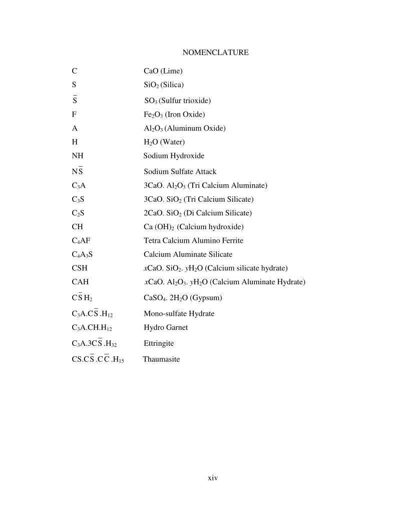
NOMENCLATURE

C CaO (Lime)

S SiO2 (Silica)

S SO3 (Sulfur trioxide)

F Fe2O3 (Iron Oxide)

A Al2O3 (Aluminum Oxide)

H H2O (Water)

NH Sodium Hydroxide

NS Sodium Sulfate Attack

C3A 3CaO. Al2O3 (Tri Calcium Aluminate)

C3S 3CaO. SiO2 (Tri Calcium Silicate)

C2S 2CaO. SiO2 (Di Calcium Silicate)

CH Ca (OH)2 (Calcium hydroxide)

C4AF Tetra Calcium Alumino Ferrite

C4A3S Calcium Aluminate Silicate

CSH xCaO. SiO2. yH2O (Calcium silicate hydrate)

CAH xCaO. Al2O3. yH2O (Calcium Aluminate Hydrate)

CS H2 CaSO4. 2H2O (Gypsum)

C3A.CS .H12 Mono-sulfate Hydrate

C3A.CH.H12 Hydro Garnet

C3A.3CS .H32 Ettringite

CS.CS .C C .H15 Thaumasite

xv

DEDICATION

I would like to dedicate this thesis

from the deepest place in my heart to my parents

H.S.Anantharaman and S.Nagapadmini,

who put the happiness and well being of their four children

ahead of their own interests for the greater part of their lives.

It is to them that I owe my good fortune in life.

xvi

ACKNOWLEDGMENTS

I would like to express my deep and sincere gratitude to my adviser, mentor and

chair of the committee, Dr. Barzin Mobasher, for providing me the opportunity to work

under him at Arizona State University. He has been actively interested in my work and

has always been available to advise me. I am very grateful for his support, patience,

motivation, and immense knowledge in cement chemistry and modeling techniques that

made my thesis work possible.

I would also like to thank my committee members Dr. Apostolos Fafitis and

Dr. Claudia Zapata for taking time to serve on my committee and give their valuable

advice for the completion of this thesis.

I would like to thank Salt River Project (SRP) for their financial support and the fly

ash samples without which this thesis would not be possible. I would also like to thank

Mr. Jeff Hearne of Salt River Materials Group (SRMG) for the supply of cement and his

help in chemical analysis of the raw flyash and cement samples.

I am very thankful to Peter Goguen, Jeffrey Long and Danny Clevenger for the

perpetual energy and enthusiasm they showed in teaching me to conduct experiments.

I would also like to thank my family and friends for their constant support and

motivation. I would like to extend my special thanks to Amir Bonakdar and Juan Alfredo

Erni, as they were my source of inspiration throughout my graduate studies and research

work. I would also like to thank my roommates for their great company during my

graduate studies here at ASU. Last but not the least, I would like to thank my sister Divya

who never let me miss my family and encouraged me in every step during my graduate

studies here at ASU.

1. INTRODUCTION

1.1. Overview

Most people do not realize that durability and strength are not synonymous when

talking about concrete. Durability is the ability to maintain integrity and strength over

time. Strength is only a measure of the ability to sustain loads at a given point in time.

Two concrete mixes with equal cylinder breaks of 4,000 psi at 28 days can vary widely in

their permeability, resistance to chemical attack, resistance to cracking and general

deterioration over time, all of which are important to durability.

Fly ash is a pozzolanic material. A Pozzolan is defined by the American Society for

Testing and Materials (ASTM) as “a siliceous or siliceous and aluminous material which

in itself possesses little or no cementitious value but which will, in finely divided form

and in the presence of moisture, chemically react with calcium hydroxide at ordinary

temperature to form compounds possessing cementitious properties.”[1]. Fly ash has been

successfully used in Portland cement concrete (PCC) as a mineral admixture for nearly

60 years, and more recently as a component of blended cement. The principal benefits

ascribed to the use of fly ash in concrete include enhanced workability due to the

spherical shape of the fly ash particle, reduced bleeding and less water demand, increased

ultimate strength, reduced permeability, lower heat of hydration, greater resistance to

sulfate attack, greater resistance to alkali-silica reaction, and reduced shrinkage. [5]

2

1.2. Problem Statement

Today, there is a general trend to replace higher levels of Portland cement with fly

ash in concrete. The increased pressure to use higher levels of fly ash in concrete systems

is due to three main reasons.

� The first reason being the economical aspect. As the replacement level of fly ash

increases, the cost to produce concrete decreases.

� The second reason and arguably the most important is the environment aspect. Fly

ash is an industrial by-product, much of which is deposited in landfills if not used in

concrete. Also from an environmental perspective, the more fly ash being utilized in

concrete, the less the demand for Portland cement, the less Portland cement

production and therefore the lower CO2 emissions.

� The third and final aspect influencing the use of higher replacement levels is the

technical benefits of high volume fly ash concrete (HVFAC > 30%). HVFAC has

improved performance over ordinary Portland cement concrete, especially in terms of

durability when appropriately used.

Although there are clearly economic and environmental benefits associated with the

use of high levels of fly ash in concrete, there is relatively little information on the

behavior of such concrete and almost no guidance on its production or use.

1.3. Objective of the Study

The objective of this research was to inspect the performance of class C and F fly ash

concrete material with replacement level from 10-40 %. The overall research included

studies on the effects of sulfate attack and alkali silica reaction on time dependent

3

properties such as compressive strength and durability issues by means of Micro-

structural studies using Scanning Electron Microscope (SEM) and Energy dispersive X-

ray spectroscopy (EDS or EDX). Theoretical modeling was used to analyze the service

life and degradation (expansion) of specimen exposed to External Sulfate Attack (ESA).

The studies included different levels of fly ash replacements, different levels of water to

cementitious material ratio (W/Cm), mortar and paste specimens and different size of the

specimens.

1.4. Scope of the Study

The analysis of sulfate attack expansions was obtained from the experimental results

obtained from the average of 4 samples in each batch. 9 batches of mortar specimens and

14 paste specimens were used for this analysis.

The 9 batches of standard size (1”x1”x11”) mortar specimens were prepared with

water to cementitous material ratio of 0.6 and the 9 batches of mortar specimens

consisted of 1 batch for the control specimen, 4 batches for class C and 4 batches for

class F fly ash, the replacement levels of fly ash were considered at 10, 20, 30 and 40 %.

The 14 batches of paste specimens were prepared with water to cementitous material

ratio of 0.4 and the 14 batches of paste specimens consisted of 7 batches of the standard

size (1”x1”x11”) and 7 batches of the modified size (0.4”x0.4”x4”) paste specimens. One

batch for control specimen was used in both cases, 3 batches for class C and 3 batches for

class F fly ash. The replacement levels of fly ash were considered at 10, 20 and 30 %.

The analysis of change in compressive strength due to the degradation of sulfate

attack was obtained from the experimental result of the average of 2 samples in each

4

batch and 27 batches of mortar specimens were used for this analysis. The water to

cementitious material ratio was 0.6 for all the batches. Furthermore the compressive

strength for 2” x 6” cylinder specimens were tested at 1, 28 and 126 days.

The analysis of alkali silica reaction expansions was obtained from the experimental

results obtained from the average of 4 samples in each batch. The 9 batches of standard

size (1”x1”x11”) mortar specimens were prepared with water to cementitous material

ratio of 0.47 and the 9 batches of mortar specimens consisted of 1 batch for the control

specimen, 4 batches for class C and 4 batches for class F fly ash. The replacement levels

of fly ash was considered at 20, 25, 30 and 40 %.

The micro-structural analysis performed for sulfate attack was on the control, 20 %

class C and F paste specimens after a exposure period of 80 weeks and the micro-

structural analysis performed for the alkali silica reaction consisted of control, 20 % class

C and F mortar specimens with a exposure time of 1, 2 and 4 weeks.

1.5. Organization of Report

Chapter 1 provides the introduction, overview, problem statement, objectives, and

scope of work.

Chapter 2 presents a brief literature review, including fly ash and its engineering

properties, chemical reaction involving fly ash (pozzolanic reaction) and a brief

introduction of SEM and EDS.

Chapter 3 describes the material used (Class C and F fly ash, different sand particles

for sulfate attack and alkali silica reaction). It also provides the chemical and

microstructural properties of the materials used.

5

Chapter 4 describes the procedure adopted for the experimental work. It provides the

procedures involving sample and solution preparation, curing and exposure conditions

and the method used for calculating the length change measurements.

Chapter 5 provides a brief introduction on the theory of sulfate attack, types of sulfate

attack, the mechanism of degradation involving sulfate attack, factors effecting sulfate

attack. It also discusses in detail the results, experimental observations for both expansion

calculations and compression strength at different time intervals and the micro-structural

studies obtained for both mortar and paste specimens.

Chapter 6 provides a brief introduction on the different theories proposed for alkali

silica reaction, factors affecting alkali silica reactions such as composition of cement, fly

ash, pessimum effect and aggregate size effect. It also discusses in detail, the results of

the experimental observations for both experimental and micro-structural studies.

Chapter 7 provides a detailed explanation of the model used for the predictions of

expansion. It also provides the detailed modeling observations made during the course

period of time.

Finally, Chapter 8 provides the concluding remarks of the summarized work

presented in this thesis.

6

2. LITERATURE REVIEW

2.1. Fly Ash and its Engineering Properties

Fly ash is the finely divided residue that results from the combustion of pulverized

coal. The pulverized coal, when blown with air into the boiler's combustion chamber

immediately ignites generating heat and producing a molten mineral residue. Boiler tubes

extract the heat from the boiler, cooling the flue gas and causing the molten mineral

residue to harden and form ash. The coarse ash particles, referred to as bottom ash or

slag, fall to the bottom of the combustion chamber, while the lighter fine residue

particles, termed fly ash, remain suspended in the flue gas. Prior to exhausting the flue

gas, fly ash is captured by particulate emission control devices, such as electrostatic

precipitators (ESP) or filter fabric collectors, commonly referred to as bag houses. [5]

According to Kruger report [7] US congress has classified fly ash as the sixth most

abundant resource in The United States of America. Out of the 62 million metric tons of

fly ash produced in 2001, only 32 % (20 million metric tons) of the total produced was

used in various non-landfill applications of which only two thirds was used in the

cement/concrete industry.

Fly ash is used in concrete where cementitous or pozzolanic action, or both, is desired.

The use of fly ash in cement/concrete makes it more cost effective, environment friendly

and also improves its performance in both fresh and hardened state. [5, 6]. The principal

benefits ascribed to the use of fly ash in fresh concrete includes enhanced workability due

to the spherical fly ash particles, called cenospheres; reduction in bleeding and water

demand; and lowering the heat of hydration. The hardened concrete enhances the

7

ultimate strength, reduces permeability, reduces shrinkage and increases durability by

increasing its resistance to sulfate attack and alkali silica reaction with its pozzolanic

action. The principal precautions that need to be taken while using fly ash in concrete are

its potential to decrease the air entraining ability with high carbon content fly ashes,

thereby reducing its durability; the extended initial setting time; the reduced heat of

hydration in colder climates which set seasonal limitations and the slow initial rate of

hydration which reduces the early strength.

Figure.2.1.1 SEM for Fly ash and Cement

Fly ashes are typically finer than Portland cement and lime. As observed in Figure2.1.1,

the SEM images with the same magnifications (800x), the fly ash particles are much

smaller than the cement particles. Usually fly ash particles are silt-sized ranging from 10-

100 microns and are generally spherical in shape. Sub bituminous fly ashes (Class C) are

generally slightly coarser than bituminous fly ash (Class F).

The spherical hollow particles (As observed in Figure.2.1.1) called the cenospheres are

believed to be formed by the expansion of CO2 and H2O gases evolved from the minerals

within the coal being burnt. The predominant forces helping the formation are, however,

8

the pressure and surface tension on the melts, as well as gravity. The predominantly

spherical microscopic structure of the fly ash is related to the equilibrium of the forces on

the molten inorganic particle as it is forced up the furnace or smoke stack against gravity.

The molten particles cool down rapidly, maintaining their equilibrium shape. A similar

situation is found in spherical drops of water falling from a faucet [6]

The engineering properties of fly ash that are of a particular interest when fly ash is

used in concrete or cement as an Supplementary Cementing Material are as following [5,

8]

1. Fineness: Fineness is the primary physical characteristic of fly ash that relates to

pozzolanic activity. As the fineness increases, the pozzolanic activity can be expected

to increase.

2. Pozzolanic activity: Pozzolanic activity refers to the ability of the silica and alumina

components of fly ash to react with available calcium and/or sodium from the

hydration products of the Portland cement.

3. Workability: At a given water-cement ratio, the spherical shape of most fly ash

particles permits greater workability than that acquired with conventional concrete

mixes. When fly ash is used, the absolute volume of cement plus fly ash usually

exceeds that of cement in conventional concrete mixes. The increased ratio of solids

volume to water volume produces a paste with improved plasticity and more

cohesiveness.

4. Time of setting: When replacing up to 25 percent of the Portland cement in concrete,

all Class F fly ashes and most Class C fly ashes increase the time of setting. However,

9

some Class C fly ashes may have little effect on, or possibly even decrease, the time

of setting.

5. Bleeding: Bleeding is usually reduced because of the greater volume of fines and

lower required water content for a given degree of workability.

6. Strength Development: Both Class C and Class F fly ashes when used as SCM are

believed to be beneficial in the development of ultimate strength than that developed

by the conventional PCC concrete. It is believed that Class F fly ash has a slow rate of

strength gain in the initial time period, whereas the Class C fly ash has almost equal

or greater rate of strength gain than the conventional PCC.

7. Mix Design: American concrete institute (ACI) recommends that Class F fly ash

replacements from 15 to 25 percent of the Portland cement and Class C fly ash

replacements from 20 to 35 percent needs to be used in the mix design to get a

durable and better performing concrete.

8. Heat of Hydration : As the fly ash reacts slowly than the conventional PCC it tends to

generate less heat per unit of time Thus, the temperature rise in large masses of

concrete (such as dams) can be significantly reduced if fly ash is substituted for

cement. Class F fly ashes are generally more effective than Class C fly ashes in

reducing the heat of hydration.

9. Permeability: As the size of fly ash is much smaller than the cement the mix is much

denser there by reducing the permeability and the reduced water content also plays an

important factor. The pozzolanic reaction produced by fly ash generates additional

cementitous compounds that act to block bleed channels, filling pore space and

10

reducing the permeability of the hardened concrete. The pozzolanic reaction

consumes calcium hydroxide (Ca OH 2), which is leach able, replacing it with

insoluble calcium silicate hydrates (CSH).

10. Sulfate Attack resistance: The hydration products such as calcium hydroxide or

portlandite and alumina-bearing phases react with the cat ions such as (Sodium and

magnesium) in the presence of water to form gypsum which in turn form expansive

material called ettringite which causes the damage of concrete. When Fly ash is used

as a replacement of cement the fly ash entailing a reduction in the C3A content (i.e.,

dilution effect) and the silica present in the fly ash react with calcium hydroxide or

portlandite to form CSH thereby reducing the formation of ettringite and mitigating

sulfate attack.

11. Alkali-Silica Reaction resistance: The alkalis present in cement reacts with the silica

present in aggregates causing expansive reactions, which can in turn cause failure.

When fly ash is used as a replacement of cement the total alkalis in the mix reduces

there by mitigates ASR. The silica present in the fly ash reacts with the alkalis present

in cement to form a no expansive calcium-alkali-silica gel there by reducing free

alkalis to react with the aggregates.

Fly ashes are classified based on their chemical composition and the source from

which they have been derived. The chemical and mineral compositions vary the color

of the fly ash from brown to tan and gray to black, depending on the amount of

unburnt carbon in the fly ash. The lighter the color, lower is the carbon content.

ASTMC618 specifies two classes of fly ash for the use in concrete 1) Class C fly ash,

11

and 2) Class F fly ash. These fly ashes should satisfy some ASTMC618

specifications as specified in Table 2.1.1 for their use in concrete.

Figure.2.1.2 Class C and F Fly ash

Table 2.1.1

Specifications for fly ash in PCC. (ASTM C 618) - Class F and C

ASTMC618 Chemical Requirement Min/Max Class F Class C

SiO2 + Al2O3 + Fe2O3 min % 70 50

SO3 max % 5 5

Moisture Content max % 3 3

LOI max % 5 5

Optional Chemical Requirement

Available Alkalies max % 1.5 1.5

Physical Requirement

Fineness (+325) max % 34 34

Pozzolanic Activity / Cement (7 Days) min % 75 75

Pozzolanic Activity / Cement (28 Days) min % 75 75

Water Requirement max % 105 105

Autoclave Expansion max % 0.8 0.8

Uniformity Requirement: Density max % 5 5

Uniformity Requirement: Fineness max % 5 5

Optional Physical Requirement

Multiple Factor (LOI x Fineness) 255 --

Increase in Drying Shrinkage max % 0.03 0.03

Uniformity Requirement: Air Entraining Agent max % 20 20

Cement / Alkali Reaction: Mortar Expansion (14

Days) max % 0.01 0.01

12

2.2. Pozzolanic Reaction

The main benefit of fly ash as SCM in concrete is that it not only reduces the

amount of non-durable calcium hydroxide (lime or portlandite), but in the process

converts it into calcium silicate hydrate (CSH), which is the strongest and most durable

portion of the paste in concrete. The paste is the key to durable and strong concrete, at

full hydration; concrete made with typical cements produces approximately 1/4 pound of

non-durable lime per pound of cement in the mix. [A]

Both Class C and Class F fly ashes react in concrete in similar ways they undergo

a “pozzolanic reaction” with the lime (calcium hydroxide) created by the hydration of

cement and water, to create the same binder (calcium silicate hydrate) as cement. The

chemical reactions involved in the pozzolanic reactions are shown in equations 2.2.1 and

2.2.2 In addition, some Class C fly ashes may possess enough lime to be self-cementing,

in addition to the pozzolanic reaction with lime from cement hydration.

Tricalcium silicate + water = Calcium silicate hydrate + Calcium hydroxide

3 2 22C S 6H O CSH 3Ca(OH)+ → + …………………………………..……....….. (2.2.1)

Calcium hydroxide + silica = Tricalcium silicate + water

2 32CH S 2C S 2H+ → + …………………………………..…………......……… (2.2.2)

Pozzolanic Reaction in ESA

Fly ash reduces calcium hydroxide, which combines with sulfates to produce

gypsum. Gypsum is a material that has greater volume than the calcium hydroxide and

sulfates that combine to form it, causing damaging expansion.

13

Typical Sulfate Attack Reaction [10]

Sodium Sulfate + Calcium hydroxide + water = Gypsum

2 4 2 2 2Na SO Ca(OH) 2H O CSH 2Na(OH)+ + → + ...….....................................… (2.2.3)

Tricalcium Aluminate + Gypsum + water = Ettringite

3 2 2 3 32C A 3CSH 26H O C A.3CS.H+ + → ……………………………...……........ (2.2.4)

Pozzolanic Reaction Mitigating Sulfate Attack

2 2 3 23Ca(OH) SiO 2C S 2H O+ → + ………………………....…………………… (2.2.5)

Pozzolanic Reaction in ASR

The glass in Fly ash is itself a very high reactive fine form of silica and has the

ability to react with alkalies (Sodium or potassium) hydroxides in Portland cement paste,

making them unavailable for expansive reaction with reactive silica in certain aggregates.

Typical Alkali Silica Reaction [11]

Calcium hydroxide + silica + Sodium hydroxide + Water = Alkali silica gel

2 2 2 2 2 2Ca(OH) SiO Na(OH) H O wNa O.xCao.ySiO .zH O+ + + → ……….…....... (2.2.6)

Here the gels formed are more or less expansive depending on the CaO content.

However, the presence of calcium appears to be essential for the ASR gel to expand, the

role of which in the reaction mechanism continues to be a matter of controversy. [11]

Pozzolanic Reaction Mitigating ASR [C]

2 2 3 23Ca(OH) SiO 2C S 2H O+ → + ……….............................……………...…… (2.2.7)

Sodium hydroxide + silica = Non expansive silica gel

2 y x zyNa(OH) xSiO Na Si O (Aqueous)+ → ………..........……................……… (2.2.8)

14

2.3. SEM and EDS

SEM: Scanning Electron Microscope

SEM is a type of electron microscope capable of producing high-resolution

images of a sample surfaces. SEM does not contain objective, intermediate and projector

lenses to magnify the image as in the optical microscope. Instead magnification results

from the ratio of the area scanned on the specimen to the area of the television screen.

(http://acept.asu.edu/PiN/rdg/elmicr/elmicr.shtml)

SEM images have a characteristic three-dimensional appearance and are useful

for judging the surface structure of the sample, which makes it perfect to analyze

different elements in cement-based materials. The resolution of the SEM can approach a

few nm and it can operate at magnifications that are easily adjusted from about 10 times -

300,000 times. [12]

In the SEM, the image is formed and presented by a very fine electron beam,

which is focused on the surface of the specimen. The beam is scanned over the specimen

in a series of lines and frames called a raster, just like the (much weaker) electron beam

in an ordinary television. At any given moment, the specimen is bombarded with

electrons over a very small area. Several things may happen to these electrons, usually

they may be absorbed by the specimen and give rise to secondary electrons of very low

energy, together with X- rays.

The secondary electrons are attracted to a grid held at a low (50 volt) positive

potential with respect to the specimen. Behind the grid is a disc held at about 10 kilovolts

positive with respect to the specimen. The disc consists of a layer of scintillant coated

15

with a thin layer of aluminum. The secondary electrons pass through the grid and strike

the disc, causing the emission of light from the scintillant. The light is led down a light

pipe to a photomultiplier tube, which converts the photons of light into a voltage. Thus

the secondary electrons produced from a small area of the specimen give rise to a voltage

signal of a particular strength. The voltage is led out of the microscope column to an

electronic console, where it is processed and amplified to generate a point of brightness

on a cathode ray tube (or television) screen forming an image. In most currently available

SEM’s, the energy of the primary electron beam can range from a few hundred eV up to

30 keV. (SEM/EDS devise at the School of Materials Science, ASU was 20 keV)

Figure.2.3.1 Schematic drawing of a scanning electron microscope

16

Figure.2.3.2 SEM Chamber where the samples are loaded (http://wikipedia.org)

Figure.2.3.3 Sample SEM image taken at ASU

EDS: Energy-Dispersive X-Ray Spectroscopy

EDS also called EDX/EDAX is an analytical tool for analyzing qualitatively and

quantitatively the chemical compositional of materials. The electron beams used are

either that of the SEM or electron beam columns specially constructed for themselves.

The EDS system can detect X-rays (emitted along with the secondary electrons) only

from elements in the periodic table above beryllium, Z-4.

17

When the specimen’s atoms electrons are bombarded with electrons, they knock

some of them off in the process. A position vacated by an ejected inner shell electron is

eventually occupied by a higher-energy electron from an outer shell. To be able to do so,

however, the transferring outer electron must give up some of its energy by emitting an

X-ray.

The amount of energy released by the transferring electron depends on which shell it

is transferring from, as well as which shell it is transferring to. Furthermore, the atom of

every element releases X-rays with unique amounts of energy during the transferring

process. Thus, EDS measures the amounts of energy present in the X-rays being released

by a specimen during electron beam bombardment, Hence the identification of the atom

from which the X-ray was emitted is established.

Figure.2.3.4 Sample EDS image taken at ASU

18

3. MATERIALS USED

3.1. Cement

Commercially available Portland cement type I/II was used for the entire research.

This kind of cement is used for general use, more especially when moderate sulfate

resistance or moderate heat of hydration is desired. The chemical analysis of the cement

used is as given in the table below and it satisfies all the requirements of ASTM C150

(i.e. Total (S+A+F), Total Alkali content = (Na2O + 0.658K2O), Compressive strength

for 1, 3,7,28 days, loss of ignition, etc).

Table 3.1.1

Chemical analyses of cement used

Cement Used Cement Used

SiO2 21.62 Free Lime 0.98

Al2O3 4.06 C3S 55.41

Fe2O3 3.54 C2S 20.27

CaO 63.9 C3S/ C2S 2.73

MgO 1.4 C3A 4.78

SO3 2.81 C4AF 10.76

L.O.I. 1.42 Blaine 4260

Total ( S+A+F) 29.22 Reflect 29

Na2O 0.06 Air 9.4

K2O 0.54 Auto Clave -0.04

Total Alkali 0.415 False Set 79

Moisture Content - Initial Set 3:10

Fineness Plus 325 97.7 Final Set 4:45

Specific Gravity - 1 Day Strength (psi) 2230

Carbon Content - 3 Day Strength (psi) 4130

ASTM Classification N/A 7 Day Strength (psi) 5380

Canadian Classification N/A 28 Day Strength (psi) 6750

Sulfur check Ok

LOI check Ok

19

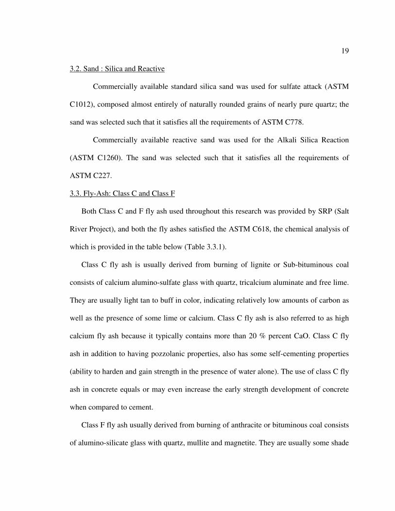
3.2. Sand : Silica and Reactive

Commercially available standard silica sand was used for sulfate attack (ASTM

C1012), composed almost entirely of naturally rounded grains of nearly pure quartz; the

sand was selected such that it satisfies all the requirements of ASTM C778.

Commercially available reactive sand was used for the Alkali Silica Reaction

(ASTM C1260). The sand was selected such that it satisfies all the requirements of

ASTM C227.

3.3. Fly-Ash: Class C and Class F

Both Class C and F fly ash used throughout this research was provided by SRP (Salt

River Project), and both the fly ashes satisfied the ASTM C618, the chemical analysis of

which is provided in the table below (Table 3.3.1).

Class C fly ash is usually derived from burning of lignite or Sub-bituminous coal

consists of calcium alumino-sulfate glass with quartz, tricalcium aluminate and free lime.

They are usually light tan to buff in color, indicating relatively low amounts of carbon as

well as the presence of some lime or calcium. Class C fly ash is also referred to as high

calcium fly ash because it typically contains more than 20 % percent CaO. Class C fly

ash in addition to having pozzolanic properties, also has some self-cementing properties

(ability to harden and gain strength in the presence of water alone). The use of class C fly

ash in concrete equals or may even increase the early strength development of concrete

when compared to cement.

Class F fly ash usually derived from burning of anthracite or bituminous coal consists

of alumino-silicate glass with quartz, mullite and magnetite. They are usually some shade

20

of gray because of the presence of unburnt carbon, with lighter shades of gray generally

indicating a higher quality of fly ash. Class F also called low calcium fly ash has less than

10% CaO. Class F fly ash has pozzolanic properties, with a little or no cementing

properties. The use of class F fly ash in concrete reduces the early strength development

of concrete.

Table 3.3.1

Chemical analyses of fly ash used

SRP Class F SRP Class C

SiO2 57.68 43.5

Al2O3 22.78 20.25

Fe2O3 5.03 6.78

CaO 6.17 16.44

MgO 1.93 3.88

SO3 0.48 1.77

L.O.I. 1.07 1

Total ( S+A+F) 85.49 70.53

Na2O 1.96 1.86

K2O 1.21 0.74

Total Alkali 2.76 2.35

Moisture Content 0.09 0.07

Fineness Plus 325 26.14 20.5

Specific Gravity 2.18 2.43

Carbon Content 0.74 0.91

ASTM Classification Class F Class C

Canadian Classification Class F Class CI

Sulfur check Ok Ok

LOI check Ok Ok

ASTM Classification:

• Class F, if total amount of SiO2+Al2O3+Fe2O3 is greater than 70%

• Class C, if total amount of SiO2+Al2O3+Fe2O3 is less than 70%

21

Canadian Classification:

• Class F, if CaO is less than 8%

• Class CI, if CaO is greater than 8% but less than 20%

• Class F, if CaO is greater than 20%

Other checks are:

• Sulfur check is Ok, if SO3 is less than 5%

• LOI check is OK, if LOI is less than 3

• R factor check is OK, if R factor is less than 2.5

3.4. Microstructural Analysis of Material Used

Cement:

Figure.3.4.1 SEM & EDS for Cement Particles

22

Figure.3.4.2 SEM & EDS for Silica Sand Particles used in Sulfate Attack

Figure.3.4.3 SEM & EDS for Reactive Sand Particles used in ASR

23

Figure.3.4.4 SEM & EDS for Class C Fly-Ash Particles

Figure.3.4.5 SEM & EDS for Class F Fly-Ash Particles

24

4. EXPERIMENTAL PROCEDURE

4.1. Introduction

This chapter details the procedures followed in the preparation of mortar/paste

specimens. The materials used and corresponding specifications are outlined. The various

test methods and test procedures are also detailed and explained. For specimens exposed

to SA, a sand to cementitious material ratio of 2.75 with water to cementitious material

ratio of 0.60 was used for mortar specimens (i.e. for mortar bars (1”x1”x11”) for ASTM

C1012 and mortar Cylinders (2” x 6”) for ASTM C109) and a sand to cementitious

material ratio of 0 with water to cementitious material ratio of 0.460 was used for the

paste specimens (i.e. for paste bars (1”x1”x11”) and ( 0.4”x0.4”x4”) for ASTM C1012 ).

For the specimens exposed to ASR, a reactive sand to cementitious material ratio of

2.25 with water to cementitious material ratio of 0.47 was used for mortar specimens (i.e.

for mortar bars (1”x1”x11”) for ASTM C1260). The reactive sand used in the mortar bars

exposed to ASR was graded as shown in the table below.

Table 4.1.1

Grading Requirements for Aggregates for ASR

Sieve Size

Passing Retained

Mass,%

4.75mm(No.4) 2.36mm(No.8) 10

2.36mm(No.8) 1.18mm(No.16) 25

1.18mm(No.16) 600µm(No.30) 25

600µm(No.30) 300µm(No.50) 25

300µm(No.50) 150µm(No.100) 15

25

4.2. Sample Preparation

4 mortar bar specimens (1”x1”x11”) were cast for each set of mix proportion for

SA and ASR, But 5-6 bar specimens of 0.4”x0.4”x4” measurement were cast for each set

of mix proportion for SA since the 0.4”x0.4”x4” specimen are very weak and easily

broken while de-molding or rough handling. 8 cylinders were cast for each set of mix

proportion specimen for SA (compression test).

Molds were prepared in accordance with ASTM C490 except the interior surfaces

of the mold were covered with releasing agents (i.e. oil in our case). The excess oil was

wiped with a dry cloth so that it does not ingress the mortar/paste specimens causing

additional reactions. Steel molds with two compartments which has provisions for

stainless steel gage studs was used for the 1”x1”x11” specimens refer to Figure 4.2.1 and

a Plexy glass molds with 4 compartments with Plexy glass studs was used for the

0.4”x0.4”x4” specimens refer to figure 4.2.2.

Figure.4.2.1 A) Steel mold for ASTM C 1012 test (11”), B) Steel stud (end pin),

C) Steel stud held in the hardened specimen.

26

Figure .4.2.2 A) Plexy glass mold for modified test, B) Plexy glass stud (end pin) details,

C) Plexy glass stud attached to the specimen.

All mortar/paste batches were mixed according to ASTM C305.The mortar/paste

mixes were mixed in an electrically driven mixer and the procedure is as following the

dry fine aggregates and cement were introduced in the mixer and blended for 60 seconds.

Then the water was slowly added to the mixer and blended for 2 minutes to thoroughly

mix all ingredients. All the molds were filled in two layers with proper compaction in

between the layers. A vibration table was used to help with the consolidation of the fresh

mixture in the molds; with the help of a travel the mortar/paste is level such that the

surface of the specimen is smooth. In accordance to ASTM C192 to prevent evaporation

of water from unhardened mortar/paste, the specimens were immediately covered with,

preferably a non-absorptive, non-reactive sheet of tough, durable impervious plastic.

27

Figure.4.2.3. Mixing, Vibrating and Casting of Specimen.

Table 4.2.1

Total Number of Specimens Prepared

Total Number of Specimens Prepared

SA (Mortar) SA (paste) ASR(Mortar)

1”x1”x11” Bars 36 28 36

0.4”x0.4”x4” Bars - 28 -

2” x 6” Cylinders 64 - -

28

4.3. Solution Preparation for SA and ASR

Sodium Hydroxide Solution for ASR: 40.0 g of NaOH was dissolved in 900 ml of water,

and was diluted with additional distilled water to obtain 1.0 L of solution. The volume

proportion of sodium hydroxide solution to the mortar bars in a storage container was

such that there were 4 ± 0.5 volumes of solution to 1 volume of mortar bars. The volume

of a mortar bar was taken as 184 ml. sufficient test solution was included to ensure

complete immersion of the mortar bars.

Figure.4.3.1 Sodium Hydroxide

Sulfate Solution for SA — 50.0 g of Na2SO4 was dissolved in 900 ml of water, and was

diluted with additional distilled water to obtain 1.0 L of solution. The solution was mixed

one day before use. The pH of the solution was determined before use; the solution with

pH outside the range of 6.0 to 8.0 was rejected. The volume proportion of sodium sulfate

solution to the mortar bars in a storage container was such that there were 4 ± 0.5

volumes of solution to 1 volume of mortar bars. The volume of a mortar bar was taken as

29

184 ml. sufficient test solution was included to ensure complete immersion of the mortar

bars.

Figure.4.3.2 Sodium Sulfate

4.4. Storage of Specimens in solution

Storage of Specimens for SA: The container containing the specimen and sodium sulfate

solution was sealed with gaffers tape to prevent evaporation from the inside. The

container was stored at room temperature of 23 ± 2°C (73.5 ± 3.5°F).

Figure.4.4.1 Sample A and Sample B Specimens in Sodium Sulfate solution

Storage of Specimens for ASR: The container for storage for ASR is chosen such that it

can withstand prolonged exposure to 80°C (176°F) and must be resistant to a 1N NaOH

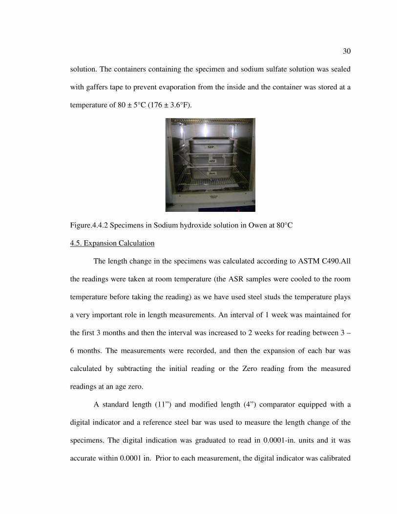
30

solution. The containers containing the specimen and sodium sulfate solution was sealed

with gaffers tape to prevent evaporation from the inside and the container was stored at a

temperature of 80 ± 5°C (176 ± 3.6°F).

Figure.4.4.2 Specimens in Sodium hydroxide solution in Owen at 80°C

4.5. Expansion Calculation

The length change in the specimens was calculated according to ASTM C490.All

the readings were taken at room temperature (the ASR samples were cooled to the room

temperature before taking the reading) as we have used steel studs the temperature plays

a very important role in length measurements. An interval of 1 week was maintained for

the first 3 months and then the interval was increased to 2 weeks for reading between 3 –

6 months. The measurements were recorded, and then the expansion of each bar was

calculated by subtracting the initial reading or the Zero reading from the measured

readings at an age zero.

A standard length (11”) and modified length (4”) comparator equipped with a

digital indicator and a reference steel bar was used to measure the length change of the

specimens. The digital indication was graduated to read in 0.0001-in. units and it was

accurate within 0.0001 in. Prior to each measurement, the digital indicator was calibrated

31

using the reference steel bar. The mortar/paste bars were all measured with the marked

date and the direction of the sample being measured for accurately obtaining comparator

readings. Figure 4.5.1 shows a mortar bar carefully positioned to measure the length

change with a digital comparator.

Figure.4.5.1 A) Digital comparator with standard steel rod,

B) Digital comparator with Sample A and Sample B specimen.

∆L = 100*Lx

LiLx −

Where,

∆L = change in length at x age, in %

Lx = comparator reading of specimen at age x – reference bar comparator reading at x

age.

Li = initial comparator or zero reading of the specimen reference bar comparator reading,

at the zero time.

32

5. SULFATE ATTACK

5.1. Introduction

Sulfate attack is among the major concrete durability and serviceability concerns

in civil infrastructure systems. It is a generic name for a set of complex and overlapping

chemical and physical processes caused by the reactions of numerous cement

components (specially the alumina-bearing components) with sulfates originating from

external or internal sources. External sources could be sulfate rich environment in the

form of sodium, potassium, magnesium and calcium sulfate and the internal sources of

sulfate could be either from cement or gypsum contaminated aggregates.

Different test methods have been developed to study the sulfate resistance of

cementitious materials, from which ASTM C 1012 is considered the most common

approach and much data is available in the literature based on the results of this test

method. This test method was followed and also modified with the following objectives:

1) To study the resistance of Class C and Class F fly ashes to sulfate attack.

2) To study the effect of different level of Class C and Class F replacement (10%-40%)

3) To study the effect of Class C and Class F ashes on the compressive strength of the

mortar cylinders subjected to sulfate attack.

4) To study the behavior and differences of mortar and paste specimens

5) To study the microstructure of specimens subjected to sulfate attack

6) To study the effect of specimen size (ASTM C1012 standard size sample A

(1”x1”x11”) and modified size sample B (0.4”x0.4”x4”)).

33

7) To calibrate a model for prediction of expansion of specimens exposed to sulfate

attack.

5.2. Literature review

5.2.1. Ettringite Formation

Secondary ettringite formation is considered to be the main cause of most of the

expansion and disruption of concrete structures involved in the sulfate attack. However,

sulfate attack is not necessarily caused by ettringite formation. When ettringite occurs

homogeneously and immediately (within hours), it does not cause any significant

disruptive action (Early Ettringite Formation, EEF). This type of harmless ettringite

formation happens, for instance, when gypsum reacts with anhydrous calcium aluminate

in the presence of water.

3 4 2 2 3 32C A 3(CaSO .2H O) 26H O C A.3CS.H+ + → ……………………..…...… (5.2.1.1)

Another example of harmless and useful EEF occurs when, under proper restraint, a

calcium aluminate sulfate (C4A3S ) hydrates within few days producing ettringite

uniformly distributed and then homogeneous expansion throughout the hardened concrete

4 3 2 4 2 2 3 32C A S 6Ca(OH ) 8(CaSO .2H O) 74H O C A.3CS.H+ + + → ……………...(5.2.1.2)

In such a case, the restrained expansion is advantageously transformed into a

rather useful stress (0.2–0.7 MPa in shrinkage-compensated concrete and 3–8 MPa in

self-stressed reinforced concretes).

On the other hand, when ettringite forms later (after several months or years) DEF

(Delayed Ettringite Formation) the related heterogeneous expansion in a very rigid

hardened concrete can produce cracking and spalling. The disruptive effect is due to the

34

non-uniform expansion localized only in the area of the concrete structure where

ettringite forms. Therefore DEF, and not EEF, is associated with a damaging sulfate

attack.

There are two different types of DEF related damage depending on the sulfate

source- external or internal sulfate attack. External sulfate attack (ESA) occurs when

environmental sulfate (from water or soil) penetrates concrete structure. Internal sulfate

attack (ISA) occurs in a sulfate-free environment where the sulfate source is inside the

concrete and comes from either cement with high sulfate content or gypsum-

contaminated aggregate.

Internal Sulfate Attack (ISA):

Modern cements, manufactured in kilns that burn sulfur-rich fuels or organic

residues - such as rubber tires - can incorporate large amounts of sulfate (up to about

2.5%) in the clinker phase, which is available for DEF formation. ISA occurs in a sulfate-

free environment when the sulfate source is inside the concrete and comes from either

cement with high sulfate content or gypsum-contaminated aggregate. The major factors

affecting ISA are: [13, 14]

1. Sulfate Content in cement: It is noticed that concrete manufactured at room

temperatures (20°C) do not show any form of ettringite-related expansion

independently of the SO3 content of the cement (2-4%). On the other hand, concrete

steam-cured at 90°C show a significant expansion related to ettringite provided that the

SO3 content of the cement is relatively high (>4%).

35

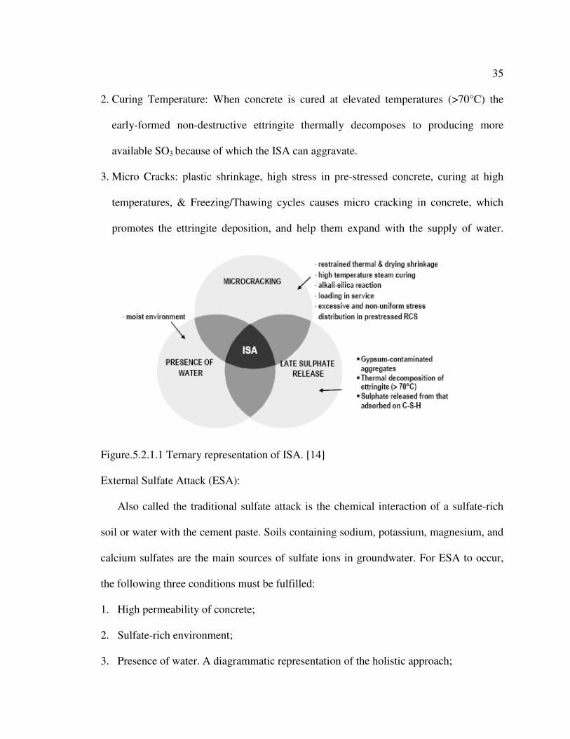
2. Curing Temperature: When concrete is cured at elevated temperatures (>70°C) the

early-formed non-destructive ettringite thermally decomposes to producing more

available SO3 because of which the ISA can aggravate.

3. Micro Cracks: plastic shrinkage, high stress in pre-stressed concrete, curing at high

temperatures, & Freezing/Thawing cycles causes micro cracking in concrete, which

promotes the ettringite deposition, and help them expand with the supply of water.

Figure.5.2.1.1 Ternary representation of ISA. [14]

External Sulfate Attack (ESA):

Also called the traditional sulfate attack is the chemical interaction of a sulfate-rich

soil or water with the cement paste. Soils containing sodium, potassium, magnesium, and

calcium sulfates are the main sources of sulfate ions in groundwater. For ESA to occur,

the following three conditions must be fulfilled:

1. High permeability of concrete;

2. Sulfate-rich environment;

3. Presence of water. A diagrammatic representation of the holistic approach;

36

Figure .5.2.1.2 Ternary representation of ESA. [14]

The ESA damage can be divided in to 3 main chemical processes. [14]

1. Sulfate attack on calcium hydroxide (CH) and calcium silicate hydrate (CSH) in the

presence of water forms gypsum.

2 2CH CSH H O CSH+ + → ………..………..…………………..…………. (5.2.1.3)

This process may cause expansion and spalling. However, its most important feature

is the loss of strength and adhesion of cement paste due to decalcification of CSH,

which is responsible for the binding capacity of the cement paste. This process may

occur with all the sulfate salts (Containing Na+, K

+, etc) except calcium or

magnesium sulfate.

2. Sulfate attack on calcium aluminate hydrates (CAH) and mono sulfate hydrate

(C3A.CS .H12) to form ettringite.

3 12 2 2 3 32CAH C A.CSH H O CSH C A.3CS.H+ + + → ……..…….………..…. (5.2.1.4)

37

This process is mainly responsible for cracking and spalling as a result of expansion

produced by DEF. This process may occur with all the sulfate salts (except MgSO4)

including calcium sulfate.

3. Sulfate attack on CSH and CH in the presence of water and carbonate ions to form

thaumasite.

4 3 2 15CSH CH SO CO H O CS.CS.CC.H+ + + + → ………..…..………….... (5.2.1.5)

The thaumasite formation is accompanied by the most severe loss of strength and

adhesion, which is able to transform hardened concrete into a pulpy mass, since a

significant part of C-S-H can be destroyed according to this reaction. This process

may occur with every type of sulfate salts and is favored by humid atmospheres and

low temperature (<10°C).

4. Sulfate attack on CSH by magnesium sulfate (MgSO4) which is not directly related to

ettringite formation but there is a loss of strength and adhesion of the cement paste

due to decalcification of CSH.

4 2 2 2 2 2CSH CH MgSO H O CSH Mg(OH) SiO xH O+ + + → + + + ………... (5.2.1.6)

5.2.2. Factors Affecting Sulfate Attack

1) Cement Type: The most important mineralogical phases of Portland cements that

affect the intensity of sulfate attack are C3A, C3S/C2S ratio and C4AF. Among the

hydration products, calcium hydroxide and alumina-bearing phases are more

vulnerable to attack by sulfate ions. On hydration, Portland cements with more than

5% tricalcium aluminate (C3A) will contain most of the alumina in the form of

monosulfate hydrate (C3A.CS .H12). If the C3A content of cement is more than 8% the

38

hydration products will also contain the hydrogarnate (C3A.CH.H12). In the presence

of calcium hydroxide, when the cement paste comes in contact with sulfate ions, both

the alumina-containing hydrates are converted to ettringite (C3A. 3CS . H32) causing

expansion and spalling. For example in a study of two type I cements with 11.9% and

9.3% of C3A with a C3S/C2S ratio of 7.88 and 2.57 respectively were investigated

for sulfate deterioration it was observed that the cement with higher C3A content had

a deterioration level 2.5 times higher than the lower C3A content. [15]

2) Cat ion Type: Sulfate attack is usually attributed to sodium, potassium, magnesium

and calcium sulfate salts. Due to the limited solubility of calcium sulfate in water at

normal temperatures (i.e., approximately 1400mg/l), It is noticed that sodium and

potassium sulfates have a very similar sulfate attack and hence it has been studied as

one by many authors hence sulfate attack can be divided in to sodium (NS A) and

magnesium sulfate (MS A) attack. It has been reported that that the strength reduction

in all blended cements exhibited superior performance in the sodium sulfate

environment (NS A) as compared with plain cements. However, the strength

reduction was very high in all the cements exposed to magnesium sulfate solution

(MS A). Further, the reduction in strength in the blended cements was more than that

in the plain cements. This is primarily due to the reduced calcium hydroxide (CH)

content in the blended cements. [15]

It has been reported that the expansions in the specimens exposed to sodium

sulfate environment (NS A) was higher when compared to those specimens exposed

to the magnesium sulfate solution (MS A). Blended cements exhibited a better

39

performance in the sodium sulfate environment (NS A) as compared with plain

cements. However the specimens with blended cements exhibited greater expansion

when compared to plain cements when exposed to magnesium sulfate solution

(MS A). [15]

3) C3S/C2S Ratio: Cements with low C3A generally have a higher C3S/C2S ratio. An

increase in C3S content of the cement generates a significantly higher quantity of

calcium hydroxide. The produced calcium hydroxide may directly combine with

sulfate ions to produce gypsum. The gypsum reduces the stiffness and cohesiveness

of the hardened cement and later gypsum also has the tendency to react with C3A to

form ettringite. For example in a study two mixes PC1 and PC2 with 7.73 % and

11.39% of C3A and C3S/C2S ratio of 4.38 and 3.58 respectively were investigated for

sulfate attack it was observed that larger expansions were sited in PC1 mix than PC2

mix. [16]

4) Effect of Temperature and Concentration: An increase in temperature of the solution

at the early ettringite formation (EEF) stage leads to a decrease in expansion for

specimens stored in the sodium sulfate solution. However, during at the delayed

ettringite formation (DEF) stage the rate of expansion was similar at all temperatures.

In the case of specimens exposed to magnesium sulfate solution, an increase in

temperatures led to an increase of the rate of expansion.

As the concentration of the solution increases the rate of expansion increases for

the specimens stored in sulfate solution at the DEF stage. However it makes no

difference at the EEF stage. In the case of specimens exposed to magnesium sulfate

40

solution the increase in concentration led to higher expansion both at EEF and DEF

stage. [17, 18]

5.3. Experimental Results and Observations

The ASTM C 1012 test method based on the evaluation of the linear expansion of

samples exposed to Sodium Sulfate Solution at room temperature was performed and the

results are presented in the following. It is mentioned that “average expansion” in the

following graphs means the average value for 4 or 5 similar specimens for each set of

paste or mortar bars.

5.3.1. Cement Mortar Sample A (1” x 1” x11”)

0 7 14 21 28

Time, Weeks

0

0.07

0.14

0.21

0.28

Av

erag

e E

xpan

sio

n,

%

ESA_ASTM-C1012 @W/Cm-0.6Sample A-1"x1"x11"

Control

Class C- 10%

Class C- 20%

Class C- 30%

Class C- 40%

NIST LIMIT

Figure.5.3.1.1 Average Expansions for Class C- Fly Ash (ESA)

41

0 7 14 21 28

Time, Weeks

0

0.07

0.14

0.21

0.28

Av

erag

e E

xpan

sio

n,

%


Control

Class F- 10%

Class F- 20%

Class F- 30%

Class F- 40%

NIST LIMIT

Figure.5.3.1.2 Average Expansions for Class F- Fly Ash (ESA)

Figures 5.3.1.1 and 5.3.1.2 show the comparison of control specimens with different

replacement levels (i.e.10, 20, 30 & 40%) of Class C and Class F fly ash respectively.

1) It was noticed that both Class C and F fly ash replaced specimens showed much

lower expansions when compared to control specimen by the end of the testing period

which is being considered as 6 months.

2) Initial expansions (i.e. time being 0-14 week’s) are such that, as the replacement level

increases the expansion increases. Though the 10% replacement of Class F showed

different trend (which was treated as a miss-fit curve).

3) It was observed that for Class C fly ash replaced specimen the replacement level has

to be greater than 10% to mitigate sulfate attack, since 10% replacement specimen did

not pass the NIST limit of 0.1% for 6 months, for all other replacement (i.e.20, 30 &

40%) the specimen passed the NIST limit of 0.1% for 6 months.

42

4) It was observed that for Class F fly ash replaced specimens the expansions of all

replacement level (i.e. 10, 20, 30 & 40%) was under the specified NIST limit of 0.1%

for 6 months though the 10% replacement specimens had expansion greater which

were considered to be a miss fit in the experimental results.

43

0 7 14 21 28

Time, Weeks

0

0.07

0.14

0.21

0.28

Av

erag

e E

xpan

sio

n,

%


Control

Class F- 10%

Class C- 10%

NIST LIMIT

Figure.5.3.1.3 Comparison Between 10 % (Class C , F ) & Control Specimen (ESA)

0 7 14 21 28

Time, Weeks

0

0.07

0.14

0.21

0.28

Av

erag

e E

xpan

sio

n,

%


Control

Class F- 20%

Class C- 20%

NIST LIMIT


44

0 7 14 21 28

Time, Weeks

0

0.07

0.14

0.21

0.28

Av

erag

e E

xpan

sio

n,

%


Control

Class F- 30%

Class C- 30%

NIST LIMIT


0 7 14 21 28

Time, Weeks

0

0.07

0.14

0.21

0.28

Av

erag

e E

xpan

sio

n,

%


Control

Class F- 40%

Class C- 40%

NIST LIMIT


45

Figures 5.3.1.3 through 5.3.1.6 shows the comparison between Control, Class C and

Class F fly ash replaced specimen with replacement levels of 10, 20, 30 & 40%

respectively.

1) It was observed that for the initial period (i.e. time being 0-14 week’s) Class F fly ash

replaced specimen showed greater expansion when compared Class C fly ash

replaced specimens Though the 10 % replacement of Class F showed different trend

(which was treated as a miss-fit curve). But after the 14th week Class F fly ash

replaced specimen mitigated expansions better when compared to Class C.

0 7 14 21 28

Time, Weeks

-0.07

0

0.07

0.14

0.21

0.28

Av

erag

e E

xp

ansi

on,

%


Control_ESA

Control_Lime Water

Figure.5.3.1.7 Comparison Between Control Specimen (ESA) and Lime Water

1) When specimens exposed to external sulfate attack was compared to specimens

exposed to lime water, it was observed that specimens exposed to lime water did not

46

have any expansion this implies that the expansions caused due to external sulfate

attack was solemnly due to the reaction products produced to cement chemistry.

5.3.2. Cement Paste Sample A (1” x 1” x11”)

0 15 30 45 60

Time, Weeks

0

0.03

0.06

0.09

0.12A

ver

age

Exp

ansi

on

, %


Control

Class C- 10%

Class C- 20%

Class C- 30%


47

0 15 30 45 60

Time, Weeks

0

0.025

0.05

0.075

0.1

Av

erag

e E

xp

ansi

on

, %


Control

Class F- 10%

Class F- 20%

Class F- 30%


Figures 5.3.2.1 and 5.3.2.2 shows the comparison of standard sized control paste

specimens with different replacement levels (i.e.10, 20 & 30%) of Class C and Class F

fly ash respectively.

1) It was observed that for standard sized paste Class C fly ash replaced specimen, the

expansion reduced as the replacement level increased and the 10% Class C fly ash

replacement specimens had greater expansions than the control specimen, this implies

that addition of Class C fly ash in lower % may worsen the ability to mitigate sulfate

attack.

2) When we compare the overall expansions of paste and mortar samples it was

observed that the expansions in mortar specimen were much greater than the paste

specimen, this is probably because of the ITZ phase in mortar and high porosity.

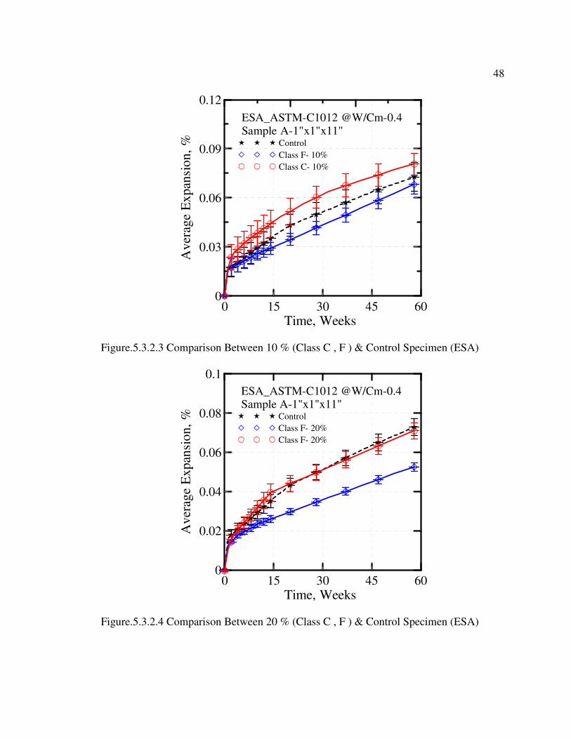
48

0 15 30 45 60

Time, Weeks

0

0.03

0.06

0.09

0.12

Av

erag

e E

xpan

sio

n,

%


Control

Class F- 10%

Class C- 10%


0 15 30 45 60

Time, Weeks

0

0.02

0.04

0.06

0.08

0.1

Av

erag

e E

xpan

sio

n,

%


Control

Class F- 20%

Class F- 20%


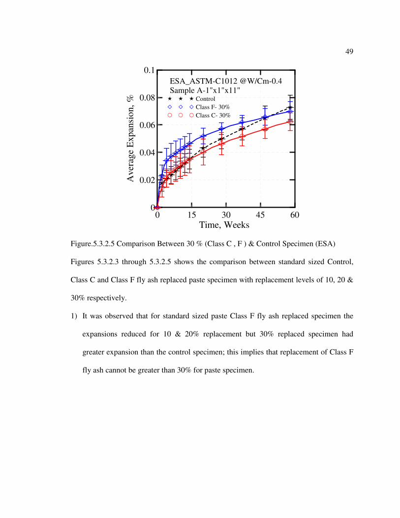
49

0 15 30 45 60

Time, Weeks

0

0.02

0.04

0.06

0.08

0.1

Aver

age

Ex

pan

sio

n,

%


Control

Class F- 30%

Class C- 30%


Figures 5.3.2.3 through 5.3.2.5 shows the comparison between standard sized Control,

Class C and Class F fly ash replaced paste specimen with replacement levels of 10, 20 &

30% respectively.

1) It was observed that for standard sized paste Class F fly ash replaced specimen the

expansions reduced for 10 & 20% replacement but 30% replaced specimen had

greater expansion than the control specimen; this implies that replacement of Class F

fly ash cannot be greater than 30% for paste specimen.

50

5.3.3. Cement paste Sample B (0.4” x 0.4” x 4”)

0 6 12 18 24

Time, Weeks

0

0.1

0.2

0.3

0.4

Av

erag

e E

xp

ansi

on

, %

ESA_ASTM-C1012 @W/Cm-0.4Sample B-0.4"x0.4"x4"

Control

Class C- 10%

Class C- 20%

Class C- 30%


0 6 12 18 24

Time, Weeks

0

0.1

0.2

0.3

0.4

Aver

age

Exp

ansi

on

, %


Control

Class F- 10%

Class F- 20%

Class F- 30%


51

Figures 5.3.3.1 and 5.3.3.2 shows the comparison of modified sized control paste

specimens with different replacement levels (i.e.10, 20 & 30%) of Class C and Class F

fly ash respectively.

1) It was observed that for modified sized Class C fly ash replaced specimen the

expansion decreased as the replacement increased, it was noticed that 10%

replacement specimen had greater expansions than the control sample, Hence Class C

fly ash cannot be used as a replacement below 20%

2) It was observed that for modified sized Class F fly ash replaced specimen the

expansion increased as the replacement increased, it was noticed that 20 & 30%

replacement specimen had greater expansions than the control sample, Hence Class F

fly ash cannot be used in greater replacement (i.e. < 20%).

0 6 12 18 24

Time, Weeks

0

0.1

0.2

0.3

0.4

Av

erag

e E

xp

ansi

on

, %


Control

Class F- 10%

Class C- 10%


52

0 6 12 18 24

Time, Weeks

0

0.1

0.2

0.3

0.4

Av

erag

e E

xp

ansi

on

, %


Control

Class F- 20%

Class C- 20%


0 6 12 18 24

Time, Weeks

0

0.1

0.2

0.3

0.4

Av

erag

e E

xp

ansi

on

, %


Control

Class F- 30%

Class C- 30%


53

Figures 5.3.3.3 through 5.3.3.5 shows the comparison between modified sized Control,

Class C and Class F fly ash replaced paste specimen with replacement levels of 10, 20 &

30% respectively.

1) It was observed that both standard and modified sized specimens follow the same

expansion trends, in both cases Class F ash replaced specimen performed better in

mitigating expansions for lower percentage levels (i.e. 10 & 20 %) whereas Class C

performed better at higher replacement levels (i.e. 30%).

5.3.4. Compression Test Mortar

0

2000

4000

6000

Com

pre

sive

Str

ength

, P

si

1 Day Strength

28 Day Strength

126 Day Strength

10% 20% 30% 40%Control

Class C Replacement

Figure.5.3.4.1 Compression Strength for Class C- Fly Ash (ESA)

54

0

1000

2000

3000

4000

5000

Com

pre

sive

Str

ength

, P

si

1 Day Strength

28 Day Strength

126 Day Strength

10% 20% 30% 40%Control

Class F Replacement

Figure.5.3.4.2 Compression Strength for Class F- Fly Ash (ESA)

Figures 5.3.4.1 and 5.3.4.2 show the comparison of compressive strength of the control

specimens with different replacement levels (i.e.10, 20, 30 & 40%) for 1, 28 & 126 days

of Class C and Class F fly ash respectively.

1) It was observed that the compressive strength of the control specimen increases

initially (i.e. for the 28th Day) but then decreases (i.e. for the 126th Day). This

reduction in strength is due to the degradation of cement matrix due to sulfate attack.

2) It was observed that the compressive strength of the Class C specimen increases with

time for the 10 & 20% but the 30 & 40% replacement levels show a initial increase

for the 28th

day but then decreases for the 126th

day. This behavior can be explained

because of the higher calcium content in Class C fly ash, which can be deleterious in

higher proportions in the cement matrix exposed to sulfate attack.

55

3) It was observed that the compressive strength of the Class F specimen increases with

time for the 30 & 40% but the 10 & 20% replacement levels show a initial increase in

compressive strength for the 28th

day but then decreases for the 126th

day.

0

1000

2000

3000C

om

pre

sive

Str

ength

, P

si

Control Specimen

Class-C Specimen

Class-F Specimen

20% 30% 40%10 %

Figure.5.3.4.3 Comparison of Compressive Strength for Class F and Class C Fly Ash

(ESA) for the 1st Day

56

0

1000

2000

3000

4000

5000

Com

pre

sive

Str

ength

, P

si

Control Specimen

Class-C Specimen

Class-F Specimen

20% 30% 40%10 %


(ESA) for the 28th

Day

0

2000

4000

6000

Com

pre

sive

Str

ength

, P

si

Control Specimen

Class-C Specimen

Class-F Specimen

20% 30% 40%10 %


(ESA) for the 126th

Day

57

Figures 5.3.4.3 through 5.3.4.5 show the comparison of compressive strength of the

control specimens with different replacement levels (i.e.10, 20, 30 & 40%) of Class C

and Class F fly ash for 1, 28 & 126 days respectively.

1) When compressive strengths of specimens exposed to sulfate solution and specimens

cured in limewater were compared it was observed that the specimens exposed to

sulfate attack had greater compressive strengths for all the curing period (i.e. 1st, 28

th

and 126th

day).

2) It was observed that for all replacement levels of Class C fly ash specimens the

compressive strength was lesser than the control specimen strength for 1st day.

3) It was observed that for 10, 20 & 30% replacement of Class F fly ash. The specimens

1st day compressive strength was almost equal to the control specimens compressive

strength for the 1st day, but for the 40% replacement of Class F fly ash had a

compressive strength much lesser than the control specimen.

4) It was observed that for all replacement levels of Class C fly ash specimens the

compressive strength for 28th

Day was greater than the control specimen compressive

strength for the 28th

day.

58

Table 5.3.4.1

Young’s Modulus for Class F Fly Ash

E=57000√f’c psi converted to GPa % Replacement

1st Day 28

th Day 126

th Day

0 16.95 GPa 23.38 GPa 21.03 GPa

10 17.36 GPa 15.78 GPa 22.08 GPa

20 16.91 GPa 23.16 GPa 22.53 GPa

30 16.43 GPa 20.96 GPa 24.36 GPa

40 12.68 GPa 20.35 GPa 25.61 GPa

Table 5.3.4.2

Strength Activity Index of Class F Fly Ash

Strength Activity Index % Replacement

1st Day 28

th Day 126

th Day

0 1 1 1

10 1.04821 0.49695471 1.10239

20 0.99484 1.07012341 1.14771

30 0.93917 0.87670778 1.36927

40 0.55968 0.82255143 1.48844

Tables 5.3.4.1 and 5.3.4.2 illustrate the young’s modulus and strength activity index of

control specimens and replacement levels (i.e.10, 20, 30 & 40%) of Class F fly ash for 1,

28 & 126 days respectively.

1) It was observed that for Class F fly ash specimen the strength activity index reduces

as the percentage level of replacement increases for 1st and 28

th day, but as the time

increases to 126th

day the strength activity increases with the increase in percentage

replacement.

59

Table 5.3.4.3

Young’s Modulus for Class C Fly Ash

E=57000√f’c in psi converted to GPa % Replacement

1st Day 28

th Day 126

th Day

0 16.95 GPa 23.38 GPa 21.03 GPa

10 15.75 GPa 23.27 GPa 25.45 GPa

20 16.02 GPa 21.77 GPa 28.02 GPa

30 15.34 GPa 23.84 GPa 22.01 GPa

40 13.96 GPa 23.59 GPa 22.43 GPa

Table 5.3.4.4

Strength Activity Index of Class C Fly Ash

Strength Activity Index % Replacement

1st Day 28

th Day 126

th Day

0 1 1 1

10 0.86341 1.0808 1.46457

20 0.89326 0.94634 1.77583

30 0.81836 1.13399 1.09549

40 0.67776 1.11095 1.13745

Tables 5.3.4.3 and 5.3.4.4 illustrate the young’s modulus and strength activity index of

control specimens and replacement levels (i.e.10, 20, 30 & 40%) of Class C fly ash for 1,

28 & 126 days respectively.

1) It was observed that for Class C fly ash specimen the strength activity was almost

equal to the control specimen for 1st and 28

th day, but as the time increased to 126

th

day, the strength activity index for lower percentage replacement levels

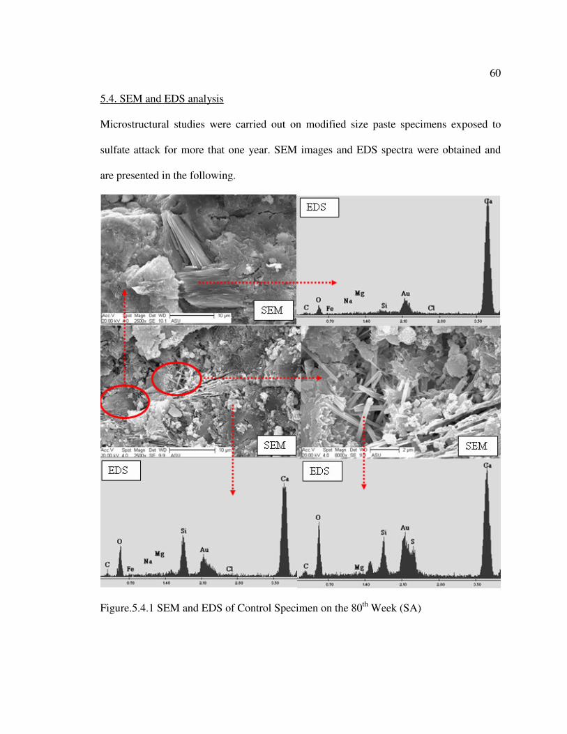
60

5.4. SEM and EDS analysis

Microstructural studies were carried out on modified size paste specimens exposed to

sulfate attack for more that one year. SEM images and EDS spectra were obtained and

are presented in the following.

Figure.5.4.1 SEM and EDS of Control Specimen on the 80th

Week (SA)

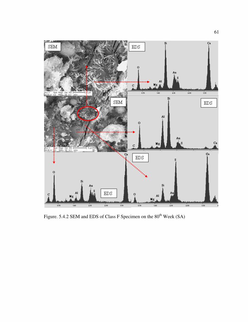
61

Figure. 5.4.2 SEM and EDS of Class F Specimen on the 80th

Week (SA)

62

Figure. 5.4.3 SEM and EDS of Class C Specimen on the 80th

Week (SA)

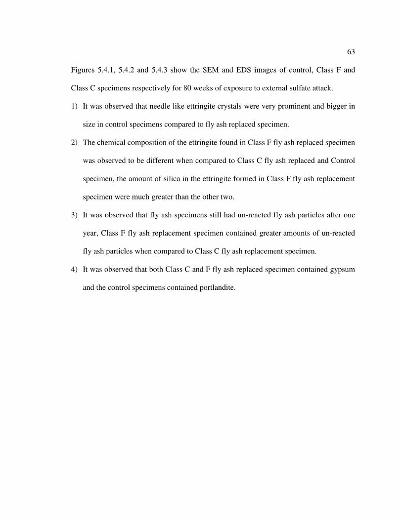
63

Figures 5.4.1, 5.4.2 and 5.4.3 show the SEM and EDS images of control, Class F and

Class C specimens respectively for 80 weeks of exposure to external sulfate attack.

1) It was observed that needle like ettringite crystals were very prominent and bigger in

size in control specimens compared to fly ash replaced specimen.

2) The chemical composition of the ettringite found in Class F fly ash replaced specimen

was observed to be different when compared to Class C fly ash replaced and Control

specimen, the amount of silica in the ettringite formed in Class F fly ash replacement

specimen were much greater than the other two.

3) It was observed that fly ash specimens still had un-reacted fly ash particles after one

year, Class F fly ash replacement specimen contained greater amounts of un-reacted

fly ash particles when compared to Class C fly ash replacement specimen.

4) It was observed that both Class C and F fly ash replaced specimen contained gypsum

and the control specimens contained portlandite.

64

5.5. Element Mapping Of Microstructure

Figure.5.5.1 EDS mapping for Control Specimen on the 80th

Week (SA)

65

Figure.5.5.2 EDS mapping for Class C Specimen on the 80th

Week (SA)

66

Figure.5.5.3 EDS mapping for Class F Specimen on the 80th

Week (SA)

67

Figures 5.5.1, 5.5.2 and 5.5.3 shows the images of element mapping of control, Class C

and Class F specimens respectively for 80 weeks of exposure to external sulfate attack.

1) It was observed that the concentration of sulfates in the scanned area of control

specimens were much greater than the concentration of sulfates found in Class C and

F fly ash replacement specimen.

2) It was observed that the concentration of calcium in Class F were greater to the

concentration of calcium observed in Class C which intern was greater than the

calcium found in the control specimen.

3) It was observed that the concentration of Class F was greater to the concentration of

aluminum in Class C. Which was also noticed in EDS spectrums for the same

specimens.

68

6. ALKALI SILICA REACTION –ASR

6.1. Introduction

An important aspect of concrete durability is its resistance to alkali aggregate

reactions (AAR), Alkali aggregate reaction (AAR) is a chemo-physical expansive

reaction in mortar or concrete between reactive mineral phases in aggregates and alkali

hydroxide and/or calcium hydroxide in the pore solution from the cement paste or from

external sources. The reaction can presently be divided in two types of reactions,

depending on the types of minerals involved 1) Alkali-Carbonate Reaction (ACR) and 2)

Alkali- Silica Reaction (ASR). [19]

1) Alkali-Carbonate Reaction (ACR) is the reaction between carbonate aggregate

particles and the cement paste of Portland cement concrete/mortar. The composition

of the carbonate rock involved determines which type of reaction occurs. Not all

carbonate reactions are deleterious the only form of ACR known to be harmful to

concrete is the "dedolomitization" reaction which may take place between

argillaceous (clay-rich) dolomitic limestone aggregate particles and the high pH of

the pore fluids in cement paste and the reaction involving in dedolomitization is as

follows.[C]

Dolomite+alkali hydroxide = brucite+calcium carbonate+ alkali carbonate

3 2 3 2 3CaMgCO 2ROH Mg(OH) CaCO R CO+ → + + ……..………...……… (6.1.1)

Alkali carbonate + calcium hydroxide = alkali hydroxide+ calcium carbonate

2 3 2 3R CO Ca(OH) 2ROH CaCO+ → + ………..……….….............……...… (6.1.2)

Where R may be any alkali (Sodium, Potassium)

69

2) Alkali silica reaction (ASR) is potentially a very disruptive reaction within concrete it

is a chemical reaction between alkali hydroxide present as the principal source in the

cement, some as the mineral constituents in the aggregate such as illitic clays, micas

or feldspars, ground water and admixtures such as deicing salts, etc. ASR reaction

produces the hydrophilic Alkali-Silica Gel (ASG) which by itself is not expansive but

this gel has a very high tendency/capacity to absorb water from the pore solution

making the pore solution more alkaline and causing the gels present in air voids and

micro crack to expand or swell which intern cause failure of the concrete. The

simplest equation which can be associated with ASR can be described as following

[19, 20]

Silicon dioxide + Alkali Hydroxide = Alkali Silica Gel + Water

2 2 4 9 24SiO 2ROH R Si O H O+ → + ………..…..………..…………...……… (6.1.3)

Where R may be any alkali (Sodium, Potassium)

During the cement hydration a certain amount of alkali ions can be released and

carried into the pore solution. When fly ashes are used in cement as SCM, they reduce the

available alkalies in the pore solution, which is called the dilution effect. Fly ashes do

contain some alkalies in them but these are mainly held in glassy structure and are not

readily available. Typically, only 16- 20 % of the total alkalis in fly ashes are water

soluble. [A]

In this thesis no distinction is made between ACR and ASR. When we use the term ASR

it is the effect of specimens exposed to NaOH solution according to ASTM C1260.

70

The aim of this work was

1) To study the resistance of Class C and Class F fly ashes as a SCM to ASR.

2) To study the effect of different level of Class C and Class F replacement (20%-40%)

3) To study the microstructure of specimen subjected to ASR.

6.2. Literature Review

Many results have been published from the experimental data on ASR and the

mitigation methods. ASTM C 1260 and C 1293 have been traditionally used for short

term and long-term test of ASR, respectively.

6.2.1. Proposed Theories of ASR

Though the exact mechanism of ASR reaction is not very well understood many

theories have been proposed by different researchers and in the literature review they

have been identified as following.

The hydroxyl ions (OH-) attacks the reactive aggregate and provokes its dissolution,

this dissolved silica reacts with alkalis (Na+ or K

+) to form alkali-silica gel (ASR Gel).

1) The expansion of concrete is due to the osmotic pressure generated by alkali silica

gels, which are confined within a semi permeable membrane of cement paste [25].

2) The expansion is a consequence of the formation and subsequent widening of cracks

due to mechanical pressure exerted by the reaction products [26].

3) The expansion of concrete depends on the type of reaction products, i.e. swelling

alkali-silica gel or non-swelling lime-alkali-silica gel. Expansion will occur only

when the swelling alkali-silica gel is formed. The Ca++ ion concentration in concrete

controls the formation of the type of reaction products [27] [28].

71

4) Different theory has been proposed by Chatterji, the main points of which are

delineated as follows: i) During the reaction, OH-, Na

+, K

+ and Ca

++ ions penetrate

reactive grains. The rate of penetration is determined by the size of the ions in

solution. ii). More Ca++ ions are left in the liquid phase because their size is larger.

iii) During the penetration, some fraction of the silica is set free to migrate away from

its original site. (iv) The concentration of Ca++ in the environment controls the rate at

which dissolved silica diffuses out of the grains. (v) An expansion occurs if more

materials penetrate a reactive grain than silica migrates out of the grains.[29]

6.2.2. Pessimum Effect and Aggregate Size Effect

An interesting feature of ASR is that expansion, which depends on the amount of

reactive silica in the aggregate, usually shows a maximum value at some intermediate

proportion of the reactive silica. At low levels of reactive silica increasing the amount

increases the expansion, but at some amount the expansion peaks, and at high levels of

reactive silica increasing the amount decreases the expansion. This is termed a pessimum

effect, because expansion is greatest, or pessimum, at this intermediate proportion of

reactive silica. [21]

A similar feature is observed with particle size of the reactive aggregate. Large sized

particles (say, centimeters in diameter) are slow to react and produce little expansion, at

least at early ages. Crushing the same material to sand size (millimeters in diameter)

speeds up the reaction and produces more expansion at early ages. Grinding the same

material to a powder (micrometers in diameter) fundamentally changes the chemical

reaction, producing calcium silicate hydrate (a normal hydration product of Portland

72

cement), which has little tendency to adsorb water and swell, instead of alkali silica gel,

so expansion is reduced. Materials that are reactive as sands are pozzolanic as powders.

[21]

6.2.3. Effect of SCM and Its Composition on ASR

The utilization of supplementary cementing materials (SCM) example fly ash, silica

fume etc. is one of the most popular ways to minimize the deleterious expansions due to

alkali–silica reaction (ASR). The precise mechanisms by which SCM suppresses

expansion are poorly understood, and the role of SCM has been variously attributed to

the following:

(1) Reduction in pore solution alkalinity

(2) Reduced availability of calcium

(3) Refined pore structure leading to reduced ionic mobility and water permeability.

Pore solution studies have shown the effect of SCM on the alkalis available in

solution to vary depending on the composition of the ash, level of replacement,

age of sample, and alkali content of the cement. [23]

The hydration products of cement-fly ash systems to bind alkalis is a function of the

CaO content of the fly ash, the binding increasing as the calcium content decreases.

However, concerning the long-term effectiveness of SCM against ASR, there are reports

stating that no deleterious expansion has been observed at the Lower Notch dam,

Northern Ontario (Canada), built with a reactive argillite and 20% fly ash, after more than

20 years, some dams built in Britain more than 50 years ago with reactive aggregates and

SCM are still in excellent condition. [19]

73

6.2.4. Effect of Cement composition on ASR

Alkali oxides such as K2O and Na2O are identified as the most significant

contributors to ASR expansion with a less strong correlation to SO3 content. The sodium

and potassium in cement are present as sulfate phases or contained within the aluminate

and silicate phases of the anhydrous cement. More than half of the alkalis not in sulfate

form are found in the C3A, C3S and ferrite in the cement higher concentrations of alkalis

(K or Na) in the pore water solution encourage greater swelling capacities in the gel. The

concentration of sodium and potassium compounds and hydroxyl ions is dependent on

the quantity of sodium and potassium compounds in the anhydrous Portland cement. The

hydroxyl ion concentration in the pore solution of concrete made with high alkali cement

may be ten times as high as that made with low alkali cement. [30]

Studies have shown that free Ca(OH)2 is a requirement for ASR to occur, although

the reactive silica may continue to dissolve without free Ca(OH)2. There appears to be a

correlation between the C/S ratio of C-S-H in portland-cement pastes and potential

deterioration from ASR. Binding C-S-H compounds with lower C/S ratios (or cements

with lower C3S/C2S ratios) are not as susceptible to deterioration as higher C/S ratio C-

S-H compounds and higher silica content binders may increase the resistance to ASR

deterioration. Therefore, cements with lower C3S/C2S ratios produce C-S-H compounds

with lower C/S ratios, which are not as susceptible to generating and sustaining ASR

attack. [30]

74

6.3. Experimental Results

0 2 4 6

Time, Weeks

0

0.2

0.4

0.6

Aver

age

Expan

sion,

%

ASTM Limit

ASR_ASTM-1260 @W/Cm-0.47

Sample A-1"x1"x11"Control

Class C- 20%

Class C- 25%

Class C- 30%

Class C- 40%

Figure.6.3.1 Average Expansions for Class C- Fly Ash (ASR)

0 2 4 6

Time, Weeks

0

0.2

0.4

0.6

Aver

age

Expan

sion,

%

ASTM Limit

ASR_ASTM-C1260 @W/Cm-0.47


Class F - 20%

Class F - 25%

Class F - 30%

Class F - 40%

Figure.6.3.2 Average Expansions for Class F- Fly Ash (ASR)

75

Figures 6.3.1 and 6.3.2 show the comparison of control specimens with different

replacement levels (i.e.20, 25, 30 & 40%) of Class C and Class F fly ash respectively.

1) It was observed that both Class C and F fly ash specimen for all replacement levels

(i.e.20 – 40%) showed a lower expansion when compared to Control specimen

throughout the exposure time.

2) It was also observed that as the amount of flyash was increased in both Class C and

Class F fly ash specimen the overall expansion decreases.

3) It was observed that though both fly ash samples mitigated ASR, class F specimen

seems to show a much better resistant to ASR when compared to class C specimens.

0 2 4 6

Time, Weeks

0

0.2

0.4

0.6

Aver

age

Expan

sion,

%

ASTM Limit



Class F- 20%

Class C- 20%

Figure. 6.3.3 Comparison Between 20 % (Class C , F ) & Control Specimen (ASR)

76

0 2 4 6

Time, Weeks

0

0.2

0.4

0.6

Av

erag

e E

xp

ansi

on

, %

ASTM Limit

ASR_ASTM-1260 @W/Cm-0.47Sample A-1"x1"x11"

Control

Class F- 25%

Class C- 25%

Figure.6.3.4 Comparison Between 25 % (Class C, F) & Control Specimen (ASR)

0 2 4 6

Time, Weeks

0

0.2

0.4

0.6

Aver

age

Expan

sion, %

ASTM Limit



Class F- 30%

Class C- 30%

Figure. 6.3.5 Comparison Between 30 % (Class C, F) & Control Specimen (ASR)

77

0 2 4 6

Time, Weeks

0

0.2

0.4

0.6

Expan

sion,

%ASTM Limit

ASR_ASTM-1260 @W/Cm-0.47Sample A-1"x1"x11"

Control

Class F- 40%

Class C- 40%

Figure. 6.3.6 Comparison Between 40 % (Class C, F) & Control Specimen (ASR)

Figures 6.3.3 through 6.3.6 shows the comparison of expansion for the control specimens

with different replacement levels (i.e.20, 25, 30 & 40%) of Class C and Class F fly ash

respectively.

1) It was observed that for Class C fly ash specimen lower replacements (20 & 25 %)

was not useful in mitigating ASR because the specimen showed greater expansions

than the specified ASTM limit of 0.1 % expansion for 2 weeks exposure time. If class

C needs to be used as a replacement in concrete/ mortar a minimum replacement of

30 % is required to mitigate ASR.

2) It was observed that for Class F fly ash specimen all replacement level’s (i.e. 20 to

40%) showed lesser expansions than the specified ASTM limit of 0.1 % expansion

for 2 weeks of exposure time.

78

6.4. SEM and EDS Analysis

Microstructural studies were carried out on control & 30%Class F fly ash specimens

exposed to sodium hydroxide solution @ 80°C for 7, 14 & 28 days. SEM images and

EDS spectra were obtained and are presented in the following.

6.4.1. Microstructural Analysis for 7 Days of Exposure

Figure. 6.4.1.1 SEM and EDS of Control Specimen on the 7th

Day (ASR)

79

Figure. 6.4.1.2 SEM and EDS of Fly Ash Specimen on the 7th

Day (ASR)

Figures 6.4.1.1 and 6.4.1.2 show the SEM images and their EDS spectra of control and

fly ash specimen respectively for an exposure time of 7 days.

1) It was observed that the pore size (i.e. Radius of the pore) found in control specimen

were almost 200µm where as the pore size in fly ash specimen were of 30 µm.

2) In control specimen prominent ASR gel was found but in the fly ash specimen the

ASR gel layer formed were found in very small pores and were very thin.

3) Thin cracks were observed in control specimen were as the matrix of fly ash

specimen were dense and crack free.

4) The composition of ASR gel in control specimen shows greater amounts of sodium

were as in fly ash specimen aluminum was found in greater quantity compared to

sodium.

80



Day (ASR)


Day (ASR)

81




remained the same where as the pore size in fly ash specimen were bigger compared

to the 7 days of exposure.

2) It was observed that for both control and fly ash specimen the ASR gel formed for the

14th

day was much thicker than the ASR gels formed on the 7th

day.

3) The cracks observed for both control and fly ash specimen were wider for the 14th

day

compared to the cracks found on the 7th

day.

4) The composition of ASR gel in control specimen shows greater amounts of sodium

for the 14th

day compared to the 7th

day, but in the fly ash specimen it was almost the

same.

82



Day (ASR)


Day (ASR)

83




remained almost the same where as the pore size in fly ash specimen were bigger

compared to the 7 & 14 days of exposure.

2) It was observed that for both control and fly ash specimen the ASR gel formed for the

28th

day was much thicker than the ASR gels formed on the 7th

& 14th

day.

3) The cracks observed for both control and fly ash specimen became very prominent

and wider for the 28th

day compared to the cracks found on the 7th

& 14th

day.

4) The composition of ASR gel in control and fly ash specimen shows greater amounts

of sodium when compared to the 7th

& 14th

day.

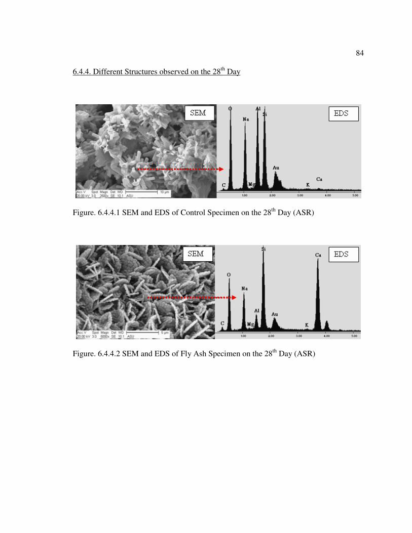
84

6.4.4. Different Structures observed on the 28th

Day


Day (ASR)


Day (ASR)

85

Figure. 6.4.4.3 AAR in Control Specimen on the 28th

Day

Figures 6.4.4.1, 6.4.4.2 and 6.4.4.3 show the SEM images and their EDS spectra of

control and fly ash specimen as mentioned for an exposure time of 28 days.

1) In control and fly ash specimens for the 28th day exposure, different kinds of crystals

were observed with almost equal amount of (Sodium (Na), Silica (Si), Aluminum

(Al) and Oxygen (o)) as ASR gels.

2) In control specimens for the 28th

day, we could observe Alkali Aggregate Reaction

(AAR) where the alkali’s (i.e. Na, sodium in our experiment) penetrated the

aggregate and caused the aggregate to crack, Other than the alkali silica gel pressure

in the pore this could be one of the means of expansion of specimen.

86

7. MODELING

7.1. Introduction

A majority of the durability issues in concrete structures deal with the diffusion of

one or several different ions into the material. Very few durability models are currently

applicable to external sulfate attack. Portland cement-based materials subjected to attack

from external sulfates may suffer from two types of damage: loss of strength of the

matrix due to degradation of C-S-H, and volumetric expansion leading to cracking. Loss

of strength has been linked to decalcification of the cement paste hydrates upon sulfate

ingress, especially of C-S-H, while cracking and expansion are attributed to formation of

expansive compounds such as gypsum or ettringite. [33]

An empirical relationship between ettringite formation and expansion is the basis for

many models where the expansive strain is linearly related to the concentration of

ettringite. This approach has been incorporated in the 4SIGHT program which predicts

the durability of concrete structures, as well as in a model that calculates the service life

of structures subjected to the ingress of sulfates by sorption or mechanical and transport

properties [37]. The work presented here uses a simplified model of the previously

developed model by R. Tixier and B. Mobasher at Arizona state University [33], [34] for

predicting the degradation of cementitious materials exposed to sulfate attack, the

literature relevant to sulfate attack modeling was reviewed and the material parameters

for the model were identified. Finally, the model predictions were compared to

experimental expansion data.

87

7.2. Simplified Model

The simplified model is presented to compute the rate of degradation and

expansion potential using a series solution approach. The model is based on the diffusion-

reaction moving boundary approach and several mechanisms for the reaction of calcium

aluminates with sulfates to form expansive ettringite are considered. There are three

major input parameters categorized under the main categories of 1) Initial Material

Parameters, 2) Size & Shape of members, and 3) Exposure & Environmental Loading.

The input parameters are used to estimate physical parameters such as the diffusivity,

strength, concentration of available calcium aluminates, and the volumetric proportions

due to chemical reactions. A schematic representation of the same is presented in the

Figure 7.2.1.

Figure. 7.2.1 The schematics of the model for sulfate attack [35]

88

Three distinct but coupled problems of sulfate diffusion, calcium aluminate

depletion, and crack front propagation are treated as a moving boundary problem as

shown in Figure 7.2.2. As the time parameter increases, the sulfates diffuse, and then

react with aluminates, resulting in hydration products which expand and potentially cause

cracking.

Figure. 7.2.2. a) Sulfate concentration profile in a specimen of length L subjected to

sulfates from at times t=0 and t>0. b) The variation of concrete diffusivity as a

function of crack front located at X=Xs [35]

It is assumed that the calcium aluminates may be a blend of three different phases of

tricalcium aluminate, tetra calcium alumino hydrate, and monosulfate with parameter γi

representing the proportion of each phase. The cement chemistry notation is used with

(C=CaO, S=SiO2, A=Al2O3, H=H2O, and S =SO3). The total calcium aluminate phase is

then introduced as: “Ca” (Ca= γ1 4 13C AH + γ2 4 12C A S H + γ3 CSH2

). Each of these

compounds may react with the ingression of sulfates (represented in the form of gypsum)

according to stoichiometric amounts defined in equations 7.2.1-7.2.3:

89

4 13 2 6 3 32C AH +3 CSH +14H C AS H +CH→ …………………….……...………….. (7.2.1)

4 12 2 6 3 32C A S H +2 CSH +16H C AS H→ ……............................................................ (7.2.2)

33 2 6 32C A +3CSH +26H C AS H→ ……………....……............................................. (7.2.3)

These reactions are lumped in a global sulfate phase-aluminate phase reaction as:

a 6 3 32C +qS C AS H→ ………………………..……..….………………………....... (7.2.4)

Where 1 2 3 2qS (3 2 3 )CSH= γ + γ + γ represents the weighted stoichiometric

coefficients of the sulfate phase. For any of the individual reactions described above, the

volumetric change due to the difference in specific gravity can be calculated.

( )( ) ( )

36 32

i 2

1C AS HV

P11

P CSHPV V

mV1

V m a m

−

−−

∆= −

+ With

k

kk

VM

dm = ………...…………………....... (7.2.5)

Where kd , kM and k

vm are respectively the density, molar mass and molar volume

of a given compound k. The concentrations of the aluminate and the sulfate phases are

represented as two parameters U and C.

4SO CAU = U and C=U ................................................................................................. (7.2.6)

The coupled differential equation for the penetration of sulfates and their reaction

with the calcium aluminate phase is represented as a first order diffusion reaction

equation and represented as:

2

2

U UD KUC

T X

∂ ∂= −

∂ ∂................................................................................................. (7.2.7)

C kUC

T q

∂= −

∂.............................................................................................................. (7.2.8)

90

Equation 7.2.7 represents the rate of change of concentration of sulfates as a

function of sulfate diffusivity and also the rate of reaction of sulfates presented as the

parameter k. Equation 7.2.8 represents the rate of reaction of Aluminate phase and since

they are assumed to be stationary in space, there is no diffusion of this phase considered.

Therefore, the change of aluminates is considered as a function of time only. It is possible

to obtain a series based solution by making simplifying assumptions regarding the

interaction of Sulfates and the Aluminate phases. If we assume that there is sufficient

amount of aluminates present so that there is no depletion of this phase, one can correlate

the rate of reaction of the Sulfates with the Aluminate phase into a single material

constant, k, representing the rate of depletion of sulfates. The higher this value the more

readily available the reaction of aluminates will be. Furthermore it is assumed that the

diffusivity remains constant and is not affected by the cracking (i.e. D1= D2) refer to

figure 7.2.2. b) Equation 7.2.7 can be simplified as a single variable second order partial

differential equation represented as Equation 7.2.9 and its series solution is represented as

equation 7.2.10 (Taken from the Crank’s Book)

2

2

U UD kU

T X

∂ ∂= −

∂ ∂.................................................................................................... (7.2.9)

[ ]( )00

U 4 1 nπX1 sin k+ν exp -T(k+ν)

U π n(k+ν) Lm

∞

=

= − ∑ ............................................... (7.2.10)

2

nπn = 2m + 1 ,ν=D

L

........................................................................................ (7.2.11)

Computation of expansion in a sample using the simplified series solution

algorithm is as follows. The solution for the series expansion of sulfate distribution is

91

obtained as a function of time for a given diffusivity and rate of reaction (D, and k= finite

amount). The baseline case for the same expression is also solved using an assumption of

k=0 (representing no Sulfate depletion due to reaction). The baseline represents the case

for the amount of sulfates that would have penetrated if there were no reactions. The

difference between the two levels is the amount of reacted sulfates as defined by

Equation 7.2.12. The average values of sulfates penetrated are obtained by integrating

the U/U0 values over the entire depth of the specimen. This level (average value of U/U0)

is multiplied by the initial sulfate concentration at the surface (ex. U0= 0.35moles/Lit,

input) to find the concentration of reacted sulfates. Stoichiometric and molar volume

relations are used to convert reacted sulfates to reacted aluminates, and ettringite formed.

Volumetric changes are related to linear expansion values. The total calcium aluminate

phase is divided into reacted and unreacted amounts and represented respectively as Car

and Cau(x,t) according to:

ar a auC (x,t)=C -C (x,t) ................................................................................................ (7.2.12)

Using a rule-of-mixtures approach, one can relate the expansive nature of the

products with the prescribed specific gravity of the compounds. In the present approach,

calculations of the volumetric changes between reactants and products were conducted by

assuming that ettringite was the only product obtained. Once the amount of reacted

calcium aluminates into ettringite as a function of time and space are obtained, they can

be related to the volumetric strain and the volume changes. It is furthermore assumed

that the crystallization pressure of products of reaction results in a bulk expansion of the

solid. The constitutive response of the matrix and the expansive stresses are calculated

92

from the imposed volumetric strain. The expansive strains are used in the constitutive

stress crack width response and an elastic equivalent stiffness is defined to account for

the reduced stiffness of the sample. An averaging scheme is used the corresponding

expansion based on the molar volumes is defined as:

t 0

V V ar

PP

∆Vε (x,t)=ε (x,t)-f Φ=C -f Φ

V

∑ ................................................................. (7.2.13)

According to equation 7.2.13, the volumetric strain is directly proportional to the

volumetric change due to the reaction products and adjusted by a shift factor representing

the total capillary porosity (Φ). Parameter f is defined as the fraction of capillary porosity

available for the dissipation of the expansion products. The magnitude of the shift

(delay) in the expansion is due to the amount of capillary porosity.

As the expansive pressures generate, localized tensile stresses are imposed on the internal

pore structure of the body. These tensile stresses are assumed to be applied to a sample

under end restrain. While a proper representation of the closing pressure profile that

normally exists in the cement based materials is needed in the formulation, in the present

case, it is assumed that the internal expansive pressures relieve the generation of closing

pressures in the vicinity of cracks. The toughening behavior, which is an inherent

component of failure in cement-based materials, is therefore lost due to the existence of

internal pressures due to the chemical reactions. The proposed procedure is based on a

simplified bridging tractions formulation. The first step is to utilize a stress crack width

relationship model. A simple uniaxial tensile stress-strain law proposed by Sakai and

Suzuki [36] is used to represent the constitutive response and represented in Equations

7.2.14 and 7.2.15. The material is assumed to be linear elastic up to the peak stress, and

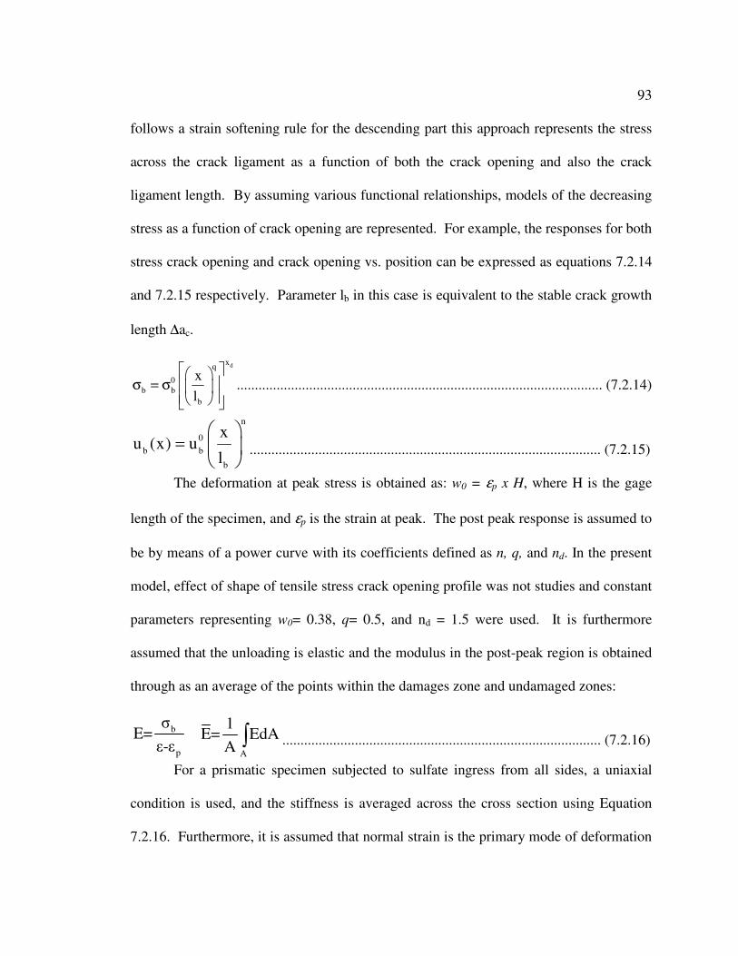
93

follows a strain softening rule for the descending part this approach represents the stress

across the crack ligament as a function of both the crack opening and also the crack

ligament length. By assuming various functional relationships, models of the decreasing

stress as a function of crack opening are represented. For example, the responses for both

stress crack opening and crack opening vs. position can be expressed as equations 7.2.14

and 7.2.15 respectively. Parameter lb in this case is equivalent to the stable crack growth

length ∆ac.

dxq

0

b b

b

x

l

σ = σ

..................................................................................................... (7.2.14)

n

0

b b

b

xu (x) u

l=

................................................................................................. (7.2.15)

The deformation at peak stress is obtained as: w0 = εp x H, where H is the gage

length of the specimen, and εp is the strain at peak. The post peak response is assumed to

be by means of a power curve with its coefficients defined as n, q, and nd. In the present

model, effect of shape of tensile stress crack opening profile was not studies and constant

parameters representing w0= 0.38, q= 0.5, and nd = 1.5 were used. It is furthermore

assumed that the unloading is elastic and the modulus in the post-peak region is obtained

through as an average of the points within the damages zone and undamaged zones:

b

p

σE=ε-ε

A

1E= EdA

A ∫ ........................................................................................ (7.2.16)

For a prismatic specimen subjected to sulfate ingress from all sides, a uniaxial

condition is used, and the stiffness is averaged across the cross section using Equation

7.2.16. Furthermore, it is assumed that normal strain is the primary mode of deformation

94

and no curvature is induced throughout the cross section. The averaged expansion is

obtained using an averaging algorithm:

Absolute expansion = i r

avg 0

1 1

E E

∆ = σ −

.............................................................. (7.2.17)

Overall expansion =

n

i

i 1=

∆ = ∆∑ ................................................................................ (7.2.18)

Parameter avgE is the average instantaneous modulus over the cross-section,

Parameter σr is assumed to be a constant uniform residual stress in the specimen due to

past history before sulfate attack such as a uniform shrinkage. In the present approach it

is assumed as 2-10 MPa, and may be viewed as the scaling parameter used to relate the

changes in the stiffness of the sample to the expansion levels observed in experiments.

95

7.3. Parameters used for Modeling

The replacement of fly ash changes the C3A content and unit weight of paste/

mortars as mentioned in the tables 7.3.1 and 7.3.2 respectively.

Table 7.3.1

Parameters Considered For Paste Specimen.

Replacement Level , W/Cm - 40 % Unit weight of

mortar

C3A

Content in %

0 % Fly ash , 100% Cement 2.5 5

10 % Fly ash, 90% Cement 2.4 4.5

20 % Fly ash, 80% Cement 2.2 4

30 % Fly ash, 70% Cement 2.0 3.5

Table 7.3.2

Parameters Considered For Mortar Specimen

Replacement Level , W/Cm - 60 % Unit weight

of mortar

C3A

Content in %

0 % Fly ash , 100% Cement 2.10 5

10 % Fly ash, 90% Cement 2.00 4.5

20 % Fly ash, 80% Cement 1.80 4

30 % Fly ash, 70% Cement 1.60 3.5

40 % Fly ash, 60% Cement 1.40 3

96

7.4. Results of Standard Size Mortar Specimen

0 46 92 138 184

Time, Days

0

0.1

0.2

0.3

Ex

pan

sio

n, %

Sulfate Attack_ASTM C10121"x1"x11" Specimen Mortar_W/Cm = 0.600% Fly ash Control

Experimental Results

Model:Parameters Used

Stage 2: Cracked

D=5x10-10 m2/sec

E0=18,E1=22 Gpa,C3A= 5 %

K=2.25x10-7 m3/mol.sec

σr= 10 Mpa, f 't= 2 Mpa

Stage 1: Uncracked

D=1x10-11 m2/sec

E0=18,E1=22 Gpa,C3A= 5 %

K=1x10-7 m3/mol.sec


Figure. 7.4.1 Modeling for 0 % Fly Ash Control - Mortar Specimen

0 46 92 138 184

Time, Days

0

0.08

0.16

0.24

Ex

pan

sio

n, %

Sulfate Attack_ASTM C10121"x1"x11" Specimen Mortar_W/Cm = 0.6010% Fly ash Replacement

Experimental Results Model:Parameters Used

Stage 2 : Cracked

D=6x10-10 m2/sec

E0=16,E1=24Gpa,C3A= 0.45 %



Stage 1 : Uncracked

D=3x10-11 m2/sec

E0=16,E1=24 Gpa,C3A=0.45 %

K=1x10-7 m3/mol.sec


Figure. 7.4.2 Modeling for 10 % Fly Ash - Mortar Specimen

97

0 46 92 138 184

Time, Days

0

0.04

0.08

0.12E

xp

ansi

on, %


Experimental Results Model:Parameters Used

Stage 2:Cracked

D=4x10-12 m2/sec

E0=16,E1=25 Gpa,C3A= 4 %


σr= 14Mpa, f 't= 2 Mpa

Stage 1:Uncracked

D=1x10-12 m2/sec

E0=16,E1=25 Gpa,C3A= 4 %




0 46 92 138 184

Time, Days

0

0.02

0.04

0.06

0.08

Ex

pan

sio

n,

%




Stage 1:Uncracked

D=8x10-12 m2/sec

E0=15,E1=26 Gpa,C3A= 3.5 %




98

0 46 92 138 184

Time, Days

0

0.02

0.04

0.06

0.08E

xp

ansi

on

, %




Stage 1:Uncracked

D=3x10-13 m2/sec

E0=14,E1=26 Gpa,C3A= 3 %




Figures 7.4.1 through 7.4.5 shows the comparison between experimental and simulation

data for 0% (Control), 10, 20, 30 & 40% fly ash mortar specimen respectively.

1) Cracking was observed only in control, 10 % and 20 % replacement specimens.

2) In control specimens the diffusivity changed by 50 times with the addition of fly ash

it was noticed that, though cracking was observed the diffusivity decreased to 25

times in the 10 % specimen and 4 times in the 20 % specimens.

3) The change in rate constant of reaction between sulfates and aluminates (i.e. K)

noticed after cracking in control, 10% & 20% is assumed to be because of the greater

surface area exposed to sulfate solution after cracking.

4) The residual hydrostatic expansive stresses (i.e.σr) in the pore microstructure

increased from 8Mpa – 10 Mpa, when cracking was observed in control, 10% & 20%

mortar specimens.

99

5) For mortar specimens it was observed that the Young's modulus of material at

exposure time (t < 28 days) (i.e. E0) decreased with the increase in the fly ash

replacement. It was observed that E0 decreased from 18 Mpa for the control specimen

to 14 Mpa for the 40 % fly ash specimen.

6) For mortar specimens it was also observed that the Young's modulus of material at

exposure time (t > 28 days) (i.e. E1) increased with the increase in the fly ash

replacement. It was observed that E1 increased from 22 Mpa for the control specimen

to 26 Mpa for the 40 % fly ash replacement specimen.

7) In general it was observed that for all mortar specimens it was noticed that the rate

constant of reaction between sulfates and aluminates (i.e. K) decreased with the

increase in fly ash replacements.

100

7.5. Results of Standard Size Paste Specimen

0 91 182 273 364

Time, Days

0

0.03

0.06

0.09

Exp

ansi

on

, %

Sulfate Attack_ASTM C10121"x1"x11" Specimen Paste_W/Cm = 0.400% Fly ash_Control


Model Parameters Used

D=5x10-11m2/sec,C3A=5%

E0=14,E1=22 Gpa


K=1.125x10-7 m3/mol.sec

Figure. 7.5.1 Modeling for Control Paste Sample-A Specimen

0 91 182 273 364

Time, Days

0

0.025

0.05

0.075

Exp

ansi

on

, %

Sulfate Attack_ASTM C10121"x1"x11" Specimen Paste_W/Cm = 0.4010% Fly ash Replacement


Model : Parameters Used

D=1x10-12 m2/sec

E0=14,E1=22 Gpa,C3A= 4.5 %

K=1x10-7 m3/mol.sec


Figure. 7.5.2 Modeling for 10 % Fly Ash Replacement Paste Sample-A Specimen

101

0 91 182 273 364

Time, Days

0

0.02

0.04

0.06

Exp

ansi

on,

%

Sulfate Attack_ASTM C10121"x1"x11" Specimen Paste_W/Cm = 0.4020% Fly ash Replacement


Model: Paramenters Used

D=5x10-13 m 2/Sec

E0=14,E1=22 Gpa,C3A= 4%

K=1e-7 m3/mol.Sec,


Figure. 7.5.3 Modeling for 20 % Fly Ash Replacement Paste Sample-A Specimen

Figures 7.5.1, 7.5.2 and 7.5.3 show the comparison between experimental and simulation

data for 0% (Control), 10 and 20% fly ash paste specimen respectively.

1) It was observed that only by changing the amount of fine aggregates, the model could

simulate expansions in agreement with the experimental results.

2) There was a greater change in diffusivity observed in paste specimen when compared

to mortar specimen. For mortar specimen the change in diffusivity (i.e. Dcontrol / D40%)

was 33.33 where as for the paste specimen the change in diffusivity (i.e. Dcontrol /

D20%) was 100.

102

7.6. Results of Modified Size Paste Specimen

0 42 84 126 168

Time, Days

0

0.1

0.2

0.3

Ex

pan

sion

, %

Sulfate Attack_ASTM C10120.4"x0.4"x4" Specimen Paste_W/Cm = 0.400% Fly ash_Control


Model: Parameters Used

D=5x10-10 m2/sec

E0=5,E1=22 Gpa,C3A= 5 %


σr= 8.5 Mpa, f 't= 2 Mpa

Figure. 7.6.1 Modeling for Control Paste Sample-B Specimen

0 42 84 126 168

Time, Days

0

0.08

0.16

0.24

Ex

pan

sion

, %

Sulfate Attack_ASTM C10120.4"x0.4"x4" Specimen Paste_W/Cm = 0.4010% Fly ash Replacment



D=9x10-11 m2/sec

E0=6,E1=24 Gpa,C3A= 4.5 %



Figure. 7.6.2 Modeling for 10 % Fly Ash Replacement Paste Sample-B Specimen

103

0 42 84 126 168

Time, Days

0

0.08

0.16

0.24

Ex

pan

sion

, %

Sulfate Attack_ASTM C10120.4"x0.4"x4" Specimen Paste_W/Cm = 0.4020% Fly ash Replacment



D=5x10-12 m2/sec

E0=7,E1=22Gpa,C3A= 4 %



Figure. 7.6.3 Modeling for 20 % Fly Ash Replacement Paste Sample-B Specimen

Figures 7.6.1, 7.6.2 and 7.6.3 show the comparison between experimental and simulation

data for the modified sized 0% (Control), 10 and 20% fly ash paste specimen

respectively.

1) One of the most critical observations was with the modeling of modified sized

specimen ( 0.4”x0.4”x4”) the Diffusion (i.e. D) and rate constant of reaction between

sulfates and aluminates (i.e. K) changed by 10 and 2.5 times respectively when

compared to standard sized specimen (1”x 1”x 11”).

This was assumed to be because of the (Surface area to volume) ratio of modified

size specimen was 2.5 times the standard size specimen as it can be observed in the

table below.

104

Table 7.7.1

Surface area to Volume Ratio of Standard and Modified Sample.

Specimen

Size

Volume V

(in.3)

Surface area

Sa (in.2)

Ratio Sa/V

1” x 1” x 11” 11 46 4.18

0.4”x0.4”x4” 0.64 6.72 10.5

Ratio =

10.5/4.18

2.52

2) The change in Young's modulus of material at exposure time (t < 28 days) (i.e. E0)

for the modified size specimen (0.4”x0.4”x4”) had to be considered for the fitting of

curves as 7 Mpa when compared to standard size specimen (1”x 1”x 11”) of 14 Mpa,

which could not be explained.

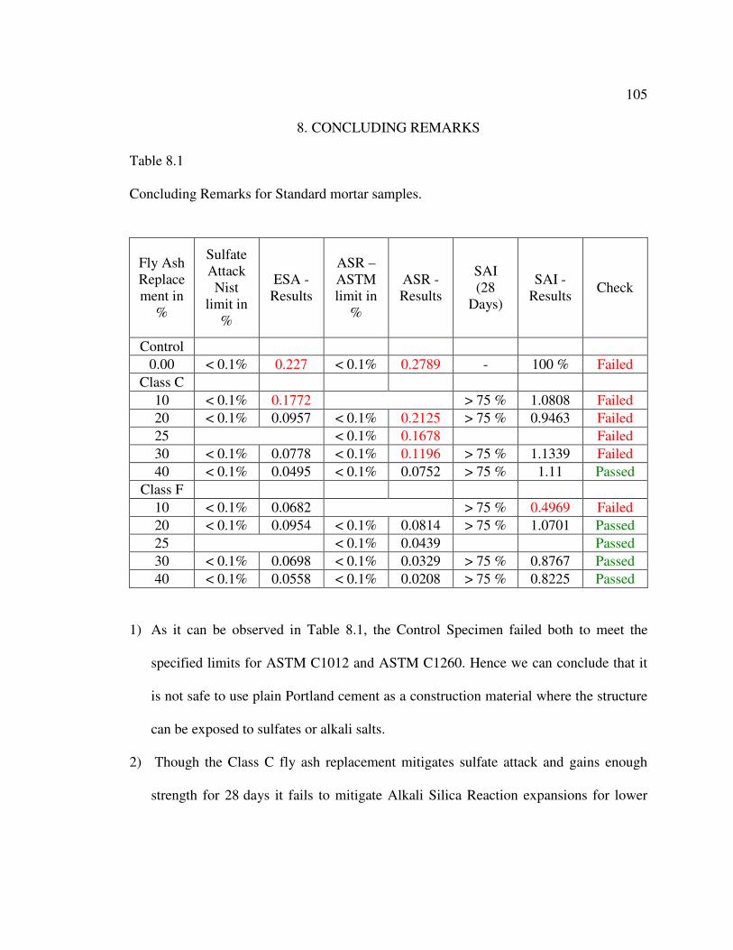
105

8. CONCLUDING REMARKS

Table 8.1

Concluding Remarks for Standard mortar samples.

1) As it can be observed in Table 8.1, the Control Specimen failed both to meet the

specified limits for ASTM C1012 and ASTM C1260. Hence we can conclude that it

is not safe to use plain Portland cement as a construction material where the structure

can be exposed to sulfates or alkali salts.

2) Though the Class C fly ash replacement mitigates sulfate attack and gains enough

strength for 28 days it fails to mitigate Alkali Silica Reaction expansions for lower

Fly Ash

Replace

ment in

%

Sulfate

Attack

Nist

limit in

%

ESA -

Results

ASR –

ASTM

limit in

%

ASR -

Results

SAI

(28

Days)

SAI -

Results Check

Control

0.00 < 0.1% 0.227 < 0.1% 0.2789 - 100 % Failed

Class C

10 < 0.1% 0.1772 > 75 % 1.0808 Failed

20 < 0.1% 0.0957 < 0.1% 0.2125 > 75 % 0.9463 Failed

25 < 0.1% 0.1678 Failed

30 < 0.1% 0.0778 < 0.1% 0.1196 > 75 % 1.1339 Failed

40 < 0.1% 0.0495 < 0.1% 0.0752 > 75 % 1.11 Passed

Class F

10 < 0.1% 0.0682 > 75 % 0.4969 Failed

20 < 0.1% 0.0954 < 0.1% 0.0814 > 75 % 1.0701 Passed

25 < 0.1% 0.0439 Passed

30 < 0.1% 0.0698 < 0.1% 0.0329 > 75 % 0.8767 Passed

40 < 0.1% 0.0558 < 0.1% 0.0208 > 75 % 0.8225 Passed

106

levels of replacements (i.e. 10 though 30 %), hence if class C fly ash needs to be used

as a replacement higher levels such as replacement more than 30 % needs to be used.

3) All % replacements of Class F fly ash (i.e.10 through 40) mitigated expansions for

both sulfate attack and Alkali silica Reaction, but it was noticed throughout the

research that the development of strength in Class F fly ash replaced specimen was

slow and low % replacements as 10 % replacement did not pass the minimum

strength requirement as specified by ASTM C618.

4) Modified samples followed similar trend to that of the standard size specimen. It was

also noticed that the Modified samples (0.4”x0.4”x4”) could produce the same

expansion in 3 months when compared to 6 months taken by the Standard samples

(1”x1”x11”), Hence by reducing the size of the specimen we can get faster and

accurate results.

REFERENCES

1. ASTM C618-92a.Standard Specification for Fly Ash and Raw or Calcined Natural

Pozzolan for Use as Mineral Admixture in Portland Cement Concrete" American

Society for Testing and Materials, Annual Book of ASTM Standards, Volume 04.02,

2. ASTM C 1012. Standard Test Method for Length Change of Hydraulic-Cement

Mortars Exposed to a Sulfate Solution, American Society for Testing and Materials,

Annual Book of ASTM Standards, Volume 04.01,

3. ASTM C1260.Standard Test Method for Potential Alkali Reactivity of Aggregates

(Mortar-Bar Method), American Society for Testing and Materials, Annual Book of

ASTM Standards, Volume 04.01,

4. ASTM C109. Standard Test Method for Compressive Strength of Hydraulic Cement

Mortars, American Society for Testing and Materials, Annual Book of ASTM

Standards, Volume 04.01,

5. American Coal Ash Association. Fly Ash Facts for Highway Engineers. Federal

Highway Administration, Report No. FHWA-SA-94-081, Washington, DC, December

1995.

6. University of Pretoria etd - Landman, AA (2003). Literature Review of Fly Ash in

Aspects of Solid-State Chemistry of Fly Ash and Ultramarine Pigments.

7. R.A.Kruger, South African Journal of science, 1986, 82,177.

8. U.S. Department of transportation, Federal highway administration. Turner-Fairbank

Highway Research Center Recycled waste Material.

9. Halstead, Woodrow J. Use of Fly Ash in Concrete. National Cooperative Highway

Research Program Synthesis of Highway Practice No. 127, Transportation Research

Board, Washington, DC, 1986.

10. Javed I. Bhatty and Peter C. Taylor, Sulfate Resistance of Concrete Using Blended

Cements or Supplementary Cementitious Materials. Portland Cement Association

2006. PCA R&D Serial No. 2916a

11. Fernandez-Jimenez, I. Garcıa-Lodeiro. Durability of alkali-activated fly ash

cementitious materials. Springer Science Business Media, LLC 2006, J Mater Sci

(2007) 42:3055–3065.

12. C. Richard Brundle, Charles A. Evans, Jr., Shaun Wilson. Encyclopedia of material

characterization. Surfaces, Interfaces, Thin Films

105

13. M.Collepardi, S. Collepardi, J.J.Ogoumah Olagot, and R.Troli, Delayed Ettringite

Formation Due to Sulfate Attack Cement Content and Curing Temperature.

14. M. Collepardi, A state-of-the-art review on delayed ettringite attack on concrete,

Cem. Concr. Compos. 25(2003) 401-407.

15. Omar S.Baghabra Al-Amoudi, Attack on plain and blended cements exposed to

aggressive sulfate environments, Cem. Concr. Compos. 24 (2002) 305–316.

16. K.Ramyar, G.Inan, Sodium Sulfate Attack on Plain and Blended Cements, Building

and Environment 42 (2007) 1368-1372.

17. Manu Santhanam, Menashi D.Cohen, Jan Olek. Mechanism of Sulfate Attack: Afresh

Look Part1: Summary of Experimental Results. Cement and Concrete Research 32

(2002) 915 – 921.

18. Manu Santhanam, Menashi D.Cohen, Jan Olek. Mechanism of Sulfate Attack: Afresh

Look Part 2: Proposed mechanisms. Cement and Concrete Research 33 (2003) 341–

346.

19. I. Sims and P. Nixon, RILEM Recommended Test Method AAR-I: Detection of

potential alkali-reactivity of aggregates-Petrographic method, RILEM TC 191-ARP

20. L.J. Malvar, G.D.Cline, D.F.Burke, R.Rolling, T.W.Sherman, and J.L.Greene, Alkali-

Silica Reaction Mitigation State-Of-The-Art and Recommendations, ACI Materials

Journal, Technical Paper Title no. 99-M49

21. George J.Z. Xu, Daniel F. Watt, Peter P. Hudec, Effectiveness of Mineral Admixture

in Reducing ASR Expansion. Cement ad Concrete Research, Vol. 25. No. 6. pp. 1225-

1236.1995

22. Medhat H.Shehata, Michael D.A.Thomas, The Effect of Fly Ash Composition on the

Expansion of Concrete due to Alkali-Silica Reaction. Cement ad Concrete Research,

30 (2000) 1063-1072.

23. Roland F. Bleszynski and Michael D.A. Thomas, Microstructural Studies of Alkali-

Silica Reaction in Fly Ash Concrete Immersed in Alkaline Solution, Advanced

Cement Based Materials 1998,7,66-78.

24. Richard Helmuth, David Stark, Sidney Diamond, Micheline Moranville-Regourd,

Alkali-Silica Reactivity an Overview of Research. Strategic Highway Research

Program, SHRP-C-342.

106

25. L. S. D Glasser, Osmotic Pressure and the Swelling of Gels. Cement at_ Concrete

Research, Vol. 9, 1979, 515-517.

26. H.E. Vivian, Studies in cement aggregate reaction: XVI. The effect of hydroxyl ions

on the reaction of opal, Australian Journal, Applied Science, 2 (1951) 108 - 113.

27. T.C. Powers, H.H. Steinour, An interpretation of some published researches on the

alkali – aggregate reaction. II. A hypothesis concerning safe and unsafe reactions

with reactive silica in concrete, American Concrete Institute journal, 26 (1955) 785–

810.

28. T.C. Powers, H.H. Steinour, An interpretation of some published researches on the

alkali–aggregate reaction: I. The chemical reactions and mechanism of expansion,

American Concrete Institute journal, 26 (1955) 497– 516.

29. S.Chatterji, N.Thaulow, and A.D.Jensen. Studies of Alkali-Silica Reaction.Part:5.

Verification of A Newly Proposed Reaction Mechanism, Cement and Concrete

Research, Mar 1989, Vol. 19, No. 2, pp 177-183.

30. Della M. Roy, Paul J. Tikalsky, Barry E. Scheetz, James Rosenberger, Tara

Cavalline, And Periaswamy Arjunan, Influence of Portland Cement Characteristics

on Alkali Silica Reactivity. TRB 2003 Annual Meeting

31. F.B.Nelson and L.J.Struble, Alkali Silica Reaction in Concrete, Center Of Excellence

for Airport Technology. Technical Note

32. Josee Duchesne, Marc-Andre Berube, Long-term effectiveness of supplementary

cementing materials against alkali–silica reaction. Cement and Concrete Research 31

(2001)1057-1063.

33. Raphael Tixier and Barzin Mobasher, Modeling of Damage in Cement-Based

Material Subjected to External Sulfate Attack. 1: Formulation, ASCE: DOI: 10.1061/

(ASCE) 0899 -1561(2003) 15:4(305).

34. Raphael Tixier and Barzin Mobasher, Modeling of Damage in Cement-Based

Material Subjected to External Sulfate Attack. 11: Comparison with Experiments,

ASCE: DOI: 10.1061/ (ASCE) 0899 -1561(2003) 15:4(314).

35. Mobasher, B. (2007), “Modeling of Stiffness Degradation and Expansion in Cement

Based Materials Subjected to External Sulfate Attack.” Materials Science of Concrete

– Transport Properties and Concrete Quality, Special Volume, American Ceramic

Society, pp. 3157-171.

107

36. Suzuki, T. and Sakai, M. (1994), A Model for Crack-Face Bridging, International

Journal of Fracture, Vol. 65, pp. 329-344.

37. B. Mobasher, and C. Ferraris, Simulation of Expansion in Cement Based Materials

Subjected to External Sulfate Attack. RILEM Technical Meeting on Durability of

Cement Based Materials, March, 2004.

BIBLIOGRAPHY

A. B. S. Choo, John Brian Newman, Advanced Concrete Technology, from Google

books.

B. Skalny, Marchand and Odler, Sulfate Attack on Concrete.

C. R.N.Swamy, the Alkali-Silica Reaction in Concrete, Department of Mechanical and

Process Engineering University of Sheffield.

D. K. Wesche, Fly Ash in Concrete, from Google books.

E. (http://acept.asu.edu/PiN/rdg/elmicr/elmicr.shtml)

APPENDIX A

ABBREVIATIONS

110

HVFAC High-Volume Fly Ash Concrete

ESA External Sulfate-Attack

ISA Internal Sulfate-Attack

AMBM The Accelerated Mortar Bar Method

EEF Early Ettringite Formation

DEF Delayed Ettringite Formation

AAR Alkali-Aggregate Reaction

AASHTO American Association of State Highway and Transportation

Officials

ACR Alkali-Carbonate Reaction

AMBT Accelerated Mortar bar Test

ASR Alkali-Silica Reaction

ASTM American Society for Testing and Materials

CPT Concrete Prism Test

SAI Strength Activity Index

DOT Department of Transportation

FHWA Federal Highway Administration

SCM Supplementary Cementitous Material

SEM Scanning Electron Microscopy

W/Cm Water To Cementitous material Ratio

ASTM C 109 Standard Test Method for Compressive Strength of Hydraulic

Cement Mortars (Using 2-in.x 4-in Cylinder Specimens)

111

ASTM C1012 Standard Test Method for Length Change of Hydraulic- Cement

Mortars Exposed to a Sulfate Solution

ASTM C 1260 The Accelerated Mortar Bar Method (AMBM) or ASTM C 1260

Standard Test Method for Potential Alkali Reactivity of

Aggregates (Mortar-Bar Method)

112

APPENDIX B

BATCHING OF SAMPLES

113

Table B.1

Sample Excel Sheet for Batching.

Sample A – dimensions Compression Test cylinders

Length, inches 11 Length, inches 4

Width, inches 1 Diameter , inches 2

Thickness, inches 1

Volume, ft3 0.006366 Volume, ft

3 0.007273

Number of samples 4 Number of samples 8

Total Volume = 0.08365 ft3

Batch Size Casting Date 3/7/2007

Volume Required+ 10% in ft3 0.092

Volume Required in cm3 2605.52

Mix Proportions (Absolute)

Cement 0.8 In %

Fine Aggregate 2.25 Times (Cement + Fly ash)

W/Cm 0.6 Times (Cement + Fly ash)

Fly ash 0.2 In %

Ingredient Specific

gravity abs vol., cm

3 weight

(Kg) Cement 3.15 402.81 1.27

Water 1 951.65 0.95

Fly ash 3 105.74 0.32

Fine Aggregates 2.5 1427.47 3.57

Total = 2887.67 5.18

Volume Required in cm3 + 10 % (Wastage)

2866.07

Volume of the material obtained based on the weight 2887.67

114

APPENDIX C

CLEANING OF GRAPHS FROM RAW DATA

115

Table C.1

Excel Sheet for Raw Data.

Date

Cast

Batch ID : C60-CF40-W/Cm47

where CF- Class F Weeks

11/10/06 Sample Measurement

Change in length of samples

in mm

1 2 3 4 1 2 3 4 0 11/12/06 -0.31 -0.03 -0.17 -0.26 0.00 0.00 0.00 0.00

0.4 11/15/06 -0.30 -0.02 -0.17 -0.24 0.01 0.01 0.01 0.02

1 11/19/06 -0.29 -0.01 -0.16 -0.23 0.01 0.02 0.02 0.02

2 11/26/06 -0.27 0.00 -0.15 -0.23 0.04 0.02 0.02 0.03

3 12/3/06 -0.27 0.00 -0.15 -0.22 0.04 0.03 0.03 0.03

4 12/10/06 -0.25 0.02 -0.13 -0.20 0.05 0.05 0.04 0.05

6 12/24/06 -0.24 0.02 -0.13 -0.20 0.06 0.05 0.05 0.06

8 1/7/07 -0.24 0.02 -0.12 -0.19 0.07 0.05 0.05 0.07

10 1/21/07 -0.23 0.02 -0.12 -0.18 0.07 0.05 0.06 0.08

12 2/4/07 -0.22 0.04 -0.10 -0.16 0.09 0.06 0.07 0.10

14 2/18/07 -0.19 0.07 -0.08 -0.12 0.12 0.10 0.09 0.13

18 3/18/07 -0.16 0.09 -0.09 0.15 0.12 0.12 0.16

22 4/15/07 -0.10 0.14 -0.02 -0.04 0.21 0.17 0.16 0.22

% of expansion = change in length

( ∆ ) / Original length *100 Samples Original

length in

mm 1 2 3 4

Average

0.000 0.000 0.000 0.000 0

1 279.09 0.003 0.003 0.002 0.005 0.003

2 279.37 0.005 0.007 0.006 0.009 0.007

3 279.23 0.013 0.008 0.007 0.010 0.009

4 279.15 0.015 0.010 0.009 0.012 0.011

0.019 0.018 0.015 0.018 0.017

0.022 0.017 0.016 0.020 0.019

0.024 0.017 0.018 0.024 0.021

0.026 0.018 0.020 0.027 0.023

0.032 0.023 0.026 0.035 0.029

0.043 0.034 0.034 0.048 0.04

0.054 0.043 0.043 0.059 0.05

0.074 0.061 0.056 0.079 0.067

116

Figure. C.1 Schematic Diagram for Cleaning up of Raw Data

sulfate and alkali silica resistance sudheen anantharaman

Documents