8 Subsurface Flow to Drains' H.P. Ritzema2

8.1 Introduction

In subsurface drainage, field drains are used to control the depth of the watertable and the level of salinity in the rootzone by evacuating excess groundwater. In this chapter, we shall use the principles of groundwater flow (Chapter 7) to describe the flow of groundwater towards the field drains. Our discussion will be restricted to parallel drains, which may be either open ditches or pipe drains. Relationships will be derived between the drain properties (diameter, depth, and spacing), the soil characteristics (profile and hydraulic conductivity), the depth of the watertable, and the corresponding discharge. To derive these relationships, we have to make several assumptions. It should be kept in mind that all the solutions are approximations; their accuracy, however, is such that their application in practice is fully justified.

We shall first discuss steady-state drainage equations (Section 8.2). These equations are based on the assumption that the drain discharge equals the recharge to the groundwater, and consequently that the watertable remains in the same position. In irrigated areas or areas with highly variable rainfall, these assumptions are not met and unsteady-state equations are sometimes more appropriate. Unsteady-state equations will be discussed in Section 8.3. In Section 8.4, we compare the steady-state approach with the unsteady state approach, and present a method in which the advantages of the two approaches are combined. Finally, in Section 8.5, we present some special drainage situations. (How the equations are to be applied in the design of subsurface drainage systems will be treated in Chapter 21 .)

8.2 Steady-State Equations

In this section, we discuss the flow of groundwater to parallel field drains under steady- state conditions. This is the typical situation in areas with a humid climate and prolonged periods of fairly uniform, medium-intensity rainfall. The steady-state theory is based on the assumption that the rate of recharge to the groundwater is uniform and steady and that it equals the discharge through the drainage system. Thus, the watertable remains at the same height as long as the recharge continues.

Figure 8.1 shows two typical cross-sections of a drainage system under these conditions. Because the groundwater is under recharge from excess rainfall, excess irrigation, or upward seepage, the watertable is curved, its elevation being highest midway between the drains. Because of the symmetry of the system (Chapter 7, Section 7.7.2), we only have to consider one half of the figure.

To describe the flow of groundwater to the drains, we have to make the following assumptions:

' based on the work carried out by J. Wesseling International Institute for Land Reclamation and Improvement

263

. . . . . . . . . . . . . . . . . . . . . . . . . . . . . . . . . . . . . . . . . . . . . . . . . . . . . . . . . . . . . . . . . . . . . . . . . . . . . . . . . . . . . . . . . . . . . . . . . . . . . . . . . . . . . . . . . . . . . . . . . . . . . . . . . . . . . . . . . . . . . . . . . . . . . . . . . . . . . . . . . . . . . . . . . . . . . . . . . . . . . . . . . . . . . . . . . . . . . . . . . . . . . . . . . . . . . . . . . . . . . . . . . . . . . . . . . . . . . . . . . . . . . . . . . . . . . . . . . . . . . . . . . . . . . . . . . . . . . . . . . . . . . . . . . . . . . . . . . . . . . . . . . . . . . . . . . . . . . . . . . . . . . . . . . . . . . . . . . . . . . . . .

i i i . . . . . . . . . . . . . . . . . . . . . . . . . . . . watertable . . . . . . . . . . . . . . . . . . . . . . . . . . . . . . . . . . . . . . . . . . .

. . . . . . . . . . . . . . . . . . . . . . . . . . . . . . . . . . . . . . . . . . . . . . . . . . . . . . . . . . . . . . . . . . . . . . . . . . . . . . . . . . . . . . . . . . . . . . . . . . . . . . . . . . . . . . . . . . . . . . . . . . . . . . . . . . . . . . . . . . . . . . . . . . . . . . . . . . . . . . . . . . . . . . . . . . . . . . . . . . . . . . . . . . . . . . . . . . . . . . . . . . . . . . . . . . . . . . . . . . . . . . . . . . . . . . . . . . . . . . . . . . . . . . . . . . . . . . . . . . . . . . . . . . . . . . . . . . . . . . . . . . . . . . . . . . . . . . . . . . . . . . . . . . . . . . . . . . . . . . . . . . . . . . . . . . . . . . . . . . . . . . . . . . . . . . . . . . . . . . . . . . . . . . . . . . . . . . .

Figure 8.1 Cross-sections of open field drains (A) and pipe drains (B), showing a curved watertable under recharge from rainfall, irrigation, or upward seepage

- Two-dimensional flow. This means that the flow is considered to be identical in any cross-section perpendicular to the drains; this is only true for infinitely long drains;

- Uniform distribution of the recharge; - Homogeneous and isotropic soils. We thus ignore any spatial variation in the

hydraulic conductivity within a soil layer, although we can treat soil profiles consisting of two or more layers.

Most drainage equations are based on the Dupuit-Forchheimer assumptions (Chapter 7, Section 7.8.1). These allow us to reduce the two-dimensional flow to a one- dimensional flow by assuming parallel and horizontal stream lines. Such a flow pattern will occur as long as the impervious subsoil is close to the drain. The Hooghoudt Equation (Section 8.2.1) is based on these conditions. If the impervious layer does not coincide with the bottom of the drain, the flow in the vicinity of the drains will be radial and the Dupuit-Forchheimer assumptions cannot be applied. Hooghoudt solved this problem by introducing an imaginary impervious layer to take into account the extra head loss caused by the radial flow. Other approximate analytical solutions were derived by Kirkham and Dagan. Kirkham (1958) presented a solution based on the potential flow theory, which takes both the flow above and below drain level into account. Toksöz and Kirkham (1961) prepared nomographs that make it easier to apply the Kirkham Equation for design purposes. The Kirkham Equation can also be used to calculate drain spacings for layered soils (Toksöz and Kirkham 1971). For

264

the calculation of drain spacings in layered soils, Walczak et al. (1988) presented an algorithm based on the Kirkham Equation. Dagan (1 964) considered radial flow close to the drain and horizontal flow further away from it. Ernst (Section 8.2.2) derived a solution for a soil profile consisting of more than one soil layer.

Of the above-mentioned equations, Hooghoudt's gives the best results (Love11 and Youngs 1984). Besides, whichever of the equations is used to calculate the drain spacings, the difference in the results will be minor in comparison with the accuracy of the input data (e.g. data on the hydraulic conductivity; see Chapter 12). We shall therefore concentrate on the Hooghoudt Equation and not further discuss the Kirkham and Dagan solutions. If, however, the soil profile consists of two or more layers with different hydraulic conductivities, we shall use the Ernst Equation.

8.2.1 The Hooghoudt Equation

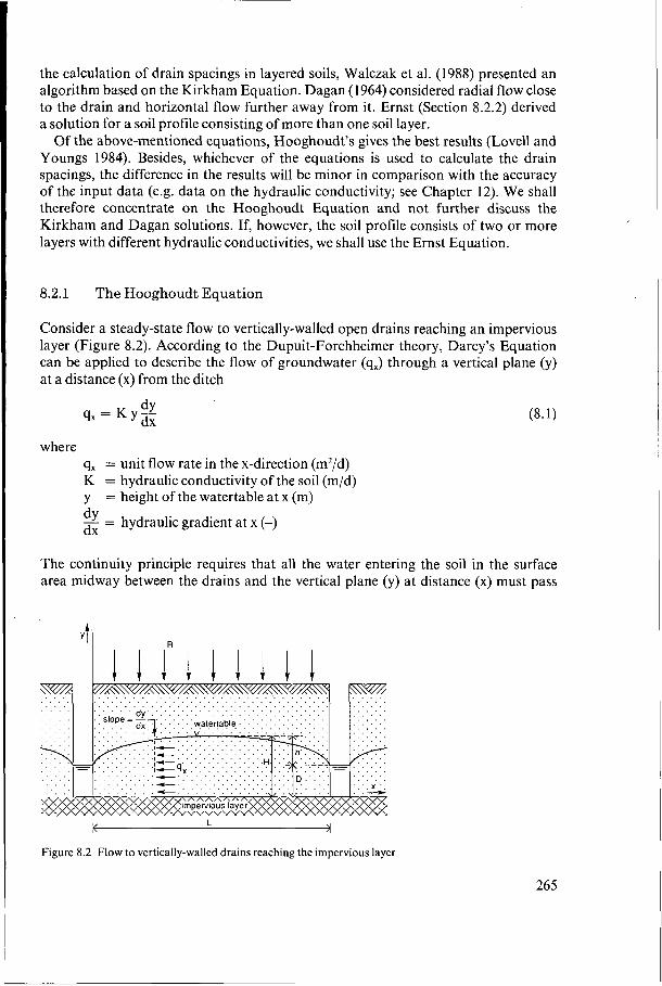
Consider a steady-state flow to vertically-walled open drains reaching an impervious layer (Figure 8.2). According to the Dupuit-Forchheimer theory, Darcy's Equation can be applied to describe the flow of groundwater (qx) through a vertical plane (y) at a distance (x) from the ditch

where q, = unit flow rate in the x-direction (m2/d) K = hydraulic conductivity of the soil (m/d) y = height of the watertable at x (m)

- = hydraulic gradient at x (-) dx dY

The continuity principle requires that all the water entering the soil in the surface area midway between the drains and the vertical plane (y) at distance (x) must pass

ulV~\UlJ,JA~,~ 1

7 . . . . . . . . . . . . . . . . . . . . . . . . . . . . . . . . . . . . . . . . . . . . . . . . . . . . . . . . . . . . . . . . . . . . . . . . .

K L 1

Figure 8.2 Flow to vertically-walled drains reaching the impervious layer

265

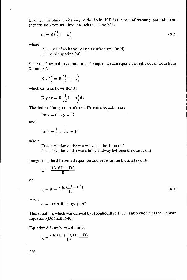
through this plane on its way to the drain. If R is the rate of recharge per unit area, then the flow per unit time through the plane (y) is

(8.2) qx = R ( ' L - ~ )

where R = rate of recharge per unit surface area (m/d) L = drain spacing (m)

Since the flow in the two cases must be equal, we can equa 8.1 and 8.2

e the right side of Equations

which can also be written as

The limits of integration of this differential equation are

for x = O --f y = D

and

1 2 for x = -L + y = H

where D = elevation of the water level in the drain (m) H = elevation of the watertable midway between the drains (m)

Integrating the differential equation and substituting the limits yields

4 k (H2 - D2) R

L2 =

or

(8.3)

where q = drain discharge (m/d)

This equation, which was derived by Hooghoudt in 1936, is also known as the Donnan Equation (Donnan 1946).

Equation 8.3 can be rewritten as

4 K (H + D) (H - D) L2 9 =

266

From Figure 8.2, it follows that H - D = h and thus H + D = 2D + h, where h is the height of the watertable above the water level in the drain. Subsequently, Equation 8.3 changes to

8 K D h + 4 K hZ L2 q =

If the water level in the drain is very low (D M O), Equation 8.4 changes to

4 K h2 q = - L2

This equation describes the flow above drain level.

(8.4)

If the impervious layer is far below drain level (D >> h), the second term in the enumerator of Equation 8.4 can be neglected, giving

8 K D h q=- L2

This equation describes the flow below drain level.

These considerations lead to the conclusion that, if the soil profile consists of two layers with different hydraulic conductivities, and if the drain level is at the interface between the soil layers, Equation 8.4 can be written as

(8.7) 8 Kb D h + 4 K, hZ

L2 q =

where K, = hydraulic conductivity of the layer above drain level (m/d) K, = hydraulic conductivity of the layer below drain level (m/d)

This situation is quite common, the soil above drain level often being more permeable

c V i t t t t I

Figure 8.3 The concept of the equivalent depth, d , to transform a combination of horizontal and radial flow (A) into an equivalent horizontal flow (B)

267

than below drain level because the soil structure above drain level has been improved by: - The periodic wetting and drying of the soil, resulting in the formation of cracks; - The presence of roots, micro-organisms, micro-fauna, etc. (This will be further elaborated in Chapter 12.)

If the pipe or open drains do not reach the impervious layer, the flow lines will converge towards the drain and will thus no longer be horizontal (Figure 8.3A). Consequently, the flow lines are longer and extra head loss is required to have the same volume of water flowing into the drains. This extra head loss results in a higher watertable.

To be able to use the concept of horizontal flow, Hooghoudt (1940) introduced two simplifications (Figure 8.3B): - He assumed an imaginary impervious layer above the real one, which decreases

the thickness of the layer through which the water flows towards the drains; - He replaced the drains by imaginary ditches with their bottoms on the imaginary

impervious layer. Under these assumptions, we can still use Equation 8.4 to express the flow towards

the drains, simply by replacing the actual depth to the impervious layer (D) with a smaller equivalent depth (d). This equivalent depth (d) represents the imaginary thinner soil layer through which the same amount of water will flow per unit time as in the actual situation. This higher flow per unit area introduces an extra head loss, which accounts for the head loss caused by the converging flow lines. Hence Equation 8.4 can be rewritten as

8 K d h + 4 K h Z LZ q =

The only problem that remains is to find a value for the equivalent depth. On the basis of the method of ‘mirror images’, Hooghoudt derived a relationship between the equivalent depth (d) and, respectively, the spacing (L), the depth to the impervious layer (D), and the radius of the drain (ra). This relationship, which is in the form of infinite series, is rather complex. Hooghoudt therefore prepared tables for the most common sizes of drain pipes, from which the equivalent depth (d) can be read directly. Table 8.1 (for ra = O. 1 m) is one such table.

As can be seen from this table, the value of d increases with D until D % &L. If the impervious layer is even deeper, the equivalent depth remains approximately constant; apparently the flow pattern is then no longer affected by the depth of the impervious layer.

Since the drain spacing L depends on the equivalent depth d, which in turn is a function of L, Equation 8.8 can only be solved by iteration. As this calculation method with the use of tables is rather time-consuming, Van Beers (1979) prepared nomographs from which d can easily be read.

Nowadays, with computers readily available, the Hooghoudt approximation method of calculating the equivalent depth can be replaced by exact solutions. A series solution developed by Van der Molen and Wesseling (1991) is presented here. Like Hooghoudt and Dagan, they analyzed the flow problem by the method of ‘mirror

268

Table 8.1 Values for the equivalent depth d of Hooghoudt for ro = 0.1 m, D and L in m (Hooghoudt 1940)

L- 5 m 7.5 10 15 20 25 30 35 40 45 50 L - 50 75 80 85 90 100 150 200 250

D D 0.5 m 0.47 0.48 0.49 0.49 0.49 0.50 0.50 0.50 0.50 0.50 0.50 0.5 0.50 0.50 0.50 0.50 0.50 0.50 0.50 0.50 0.50 0.75 0.60 0.65 0.69 0.71 0.73 0.74 0.75 0.75 0.75 0.76 0.76 1 0.96 0.97 0.97 0.97 0.98 0.98 0.99 0.99 0.99 1.00 0.67 0.75 0.80 0.86 0.89 0.91 0.93 0.94 0.96 0.96 0.96 2 1.72 1.80 1.82 1.82 1.83 1.85 1.00 1.92 1.94 1.25 0.70 0.82 0.89 1.00 1.05 1.09 1.12 1.13 1.14 1.14 1.15 3 2.29 2.49 2.52 2.54 2.56 2.60 2.72 2.70 2.83 1.50 0.70 0.88 0.97 1.11 1.19 1.25 1.28 1.31 1.34 1.35 1.36 4 2.71 3.04 3.08 3.12 3.16 3.24 3.46 3.58 3.66 1.75 0.70 0.91 1.02 1.20 1.30 1.39 1.45 1.49 1.52 1.55 1.57 5 3.02 3.49 3.55 3.61 3.67 3.78 4.12 4.31 4.43 2.00 0.70 0.91 1.08 1.28 1.41 1.5 1.57 1.62 1.66 1.70 1.72 6 3.23 3.85 3.93 4.00 4.08 4.23 4.70 4.97 5.15 2.25 0.70 0.91 1.13 1.34 1.50 1.69 1.69 1.76 1.81 1.84 1.86 7 3.43 4.14 4.23 4.33 4.42 4.62 5.22 5.57 5.81 2.50 0.70 0.91 1.13 1.38 1.57 1.69 1.79 1.87 1.94 1.99 2.02 8 3.56 4.38 4.49 4.61 4.72 4.95 5.68 6.13 6.43 2.75 0.70 0.91 1.13 1.42 1.63 1.76 1.88 1.98 2.05 2.12 2.18 9 3.66 4.57 4.70 4.82 4.95 5.23 6.09 6.63 7.00 3.00 0.70 0.91 1.13 1.45 1.67 1.83 1.97 2.08 2.16 2.23 2.29 10 3.74 4.74 4.89 5.04 5.18 5.47 6.45 7.09 7.53 3.25 0.70 ~ 0.91 1.13 1.48 1.71 1.88 2.04 2.16 2.26 2.35 2.42 12.5 3.74 5.02 5.20 5.38 5.56 5.92 7.20 8.06 8.68 3.50 0.70 0.91 1.13 1.50 1.75 1.93 2.11 2.24 2.35 2.45 2.54 15 3.74 5.20 5.40 5.60 5.80 6.25 7.77 8.84 9.64 3.75 0.70 0.91 1.13 1.52 1.78 1.97 2.17 2.31 2.44 2.54 2.64 17.5 3.74 5.30 5.53 5.76 5.99 6.44 8.20 9.47 10.4 4.00 0.70 0.91 1.13 1.52 1.81 2.02 2.22 2.37 2.51 2.62 2.71 20 3.74 5.30 5.62 5.87 6.12 6.60 8.54 9.97 11.1 4.50 0.70 0.91 1.13 1.52 1.85 2.08 2.31 2.50 2.63 2.76 2.87 25 3.74 5.30 5.74 5.96 6.20 6.79 8.99 10.7 12.1 5.00 0.70 0.91 1.13 1.52 1.88 2.15 2.38 2.58 2.75 2.89 3.02 30 3.74 5.30 5.74 5.96 6.20 6.79 9.27 11.3 12.9 5.50 0.70 0.91 1.13 1.52 1.88 2.20 2.43 2.65 2.84 3.00 3.15 35 3.74 5.30 5.74 5.96 6.20 6.79 9.44 11.6 13.4 6.00 0.70 0.91 1.13 1.52 1.88 2.20 2.48 2.70 2.92 3.09 3.26 40 3.74 5.30 5.74 5.96 6.20 6.79 9.44 11.8 13.8 7.00 0.70 0.91 1.13 1.52 1.88 2.20 2.54 2.81 3.03 3.24 3.43 45 3.74 5.30 5.74 5.96 6.20 6.79 9.44 12.0 13.8 8.00 0.70 0.91 1.13 1.52 1.88 2.20 2.57 2.85 3.13 3.35 3.56 50 3.74 5.30 5.74 5.96 6.20 6.79 9.44 12.1 14.3 9.00 0.70 0.91 1.13 1.52 1.88 2.20 2.57 2.89 3.18 3.43 3.66 60 3.74 5.30 5.74 5.96 6.20 6.79 9.44 12.1 14.6

m 0.71 0.93 1.14 1.53 1.89 2.24 2.58 2.91 3.24 3.56 3.88 10.00 0.70 0.91 1.13 1.52 1.88 2.20 2.57 2.89 3.23 3.48 3.74 m 3.88 5.38 5.76 6.00 6.26 6.82 9.55 12.2 14.7

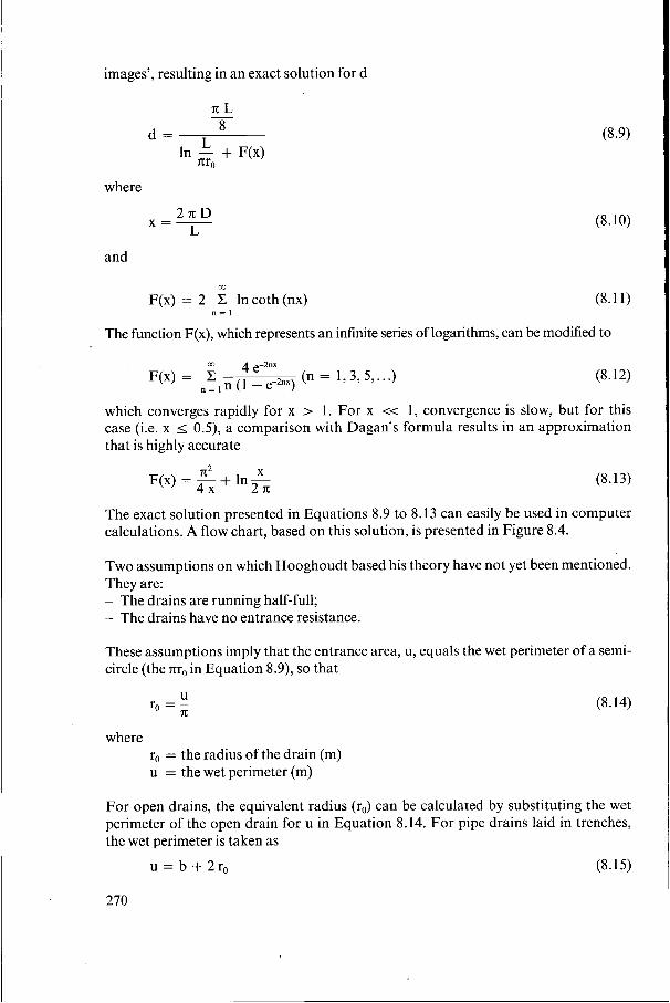
images’, resulting in an exact solution for d

71L

where

27cD L

x = -

and

m

F(x) = 2 C lncoth(nx) n = I

(8.10)

(8.11)

The function F(x), which represents an infinite series of logarithms, can be modified to

m 4 e-2n2nx F(x) = C (n = 1,3,5,. . .)

= , n (1 - e-2nx) (8.12)

which converges rapidly for x > 1. For x << 1, convergence is slow, but for this case (i.e. x 0.5), a comparison with Dagan’s formula results in an approximation that is highly accurate

79 X F(x) = - + In- 4 x 271 (8.13)

The exact solution presented in Equations 8.9 to 8.13 can easily be used in computer calculations. A flow chart, based on this solution, is presented in Figure 8.4.

Two assumptions on which Hooghoudt based his theory have not yet been mentioned. They are: - The drains are running half-full; - The drains have no entrance resistance.

These assumptions imply that the entrance area, u, equals the wet perimeter of a semi- circle (the nr0 in Equation 8.9), so that

U ro = i (8.14)

where r,, = the radius of the drain (m) u = the wet perimeter (m)

For open drains, the equivalent radius (ro) can be calculated by substituting the wet perimeter of the open drain for u in Equation 8.14. For pipe drains laid in trenches, the wet perimeter is taken as

U = b + 2rO (8.15)

270

input : D, ro,

and first estimate of L

no

4e-2nx F(x) = Z -

2 n=1.3.5...n(l-ë2nxX) F(X) = K + In X 4x 2n d = D I d = D I

I I

Figure 8.4 Flow chart for the calculation of Hooghoudt’s equivalent depth

where b = the width of the trench (m)

If an envelope material is used around the pipe drain (Figure 8.5), Equation 8.15 changes to

(8.16) u = b + 2(2r, + m)

where

m = the height of the envelope above the drain (m)

The second assumption (no entrance resistance) means that we are assuming an ideal drain. This is correct as long as the hydraulic conductivity of the drain trench is at least 10 times higher than that of the undisturbed soil outside the trench (Smedema and Rycroft 1983). If the hydraulic conductivity is less, an envelope material can be used to decrease the entrance resistance, so that a greater part of the total head will be available for the flow through the soil. If it is not possible to use an envelope material, the entrance resistance should be introduced into the equations by replacing h with (h - he), in which he is the entrance head loss in metres. The entrance resistance and the use of envelopes will be further discussed in Chapter 21.

27 1

. . . . . . . . . . . . . . . . . . . . . . . . . . . . . . . . . . . . . . . . . . . . . . . . . . . . . . . . . e b - +

Figure 8.5 Drain pipe with gravel envelope in drain trench

8.2.2 The Ernst Equation

So far, we have only discussed solutions that can be applied for a homogeneous soil profile, or for a two-layered soil profile provided that the interface between the two layers coincides with the drain level. The Ernst Equation is applicable to any type of two-layered soil profile. It has the advantage over the Hooghoudt Equation that the interface between the two layers can be either above or below drain level. It is especially useful when the top layer has a considerably lower hydraulic conductivity than the bottom layer.

To obtain a generally applicable solution for soil profiles consisting of layers with different hydraulic conductivities, Ernst (1956; 1962) divided the flow to the drains into a vertical, a horizontal, and a radial component (Figure 8.6). Consequently, the total available head (h) can be divided into a head loss caused by the vertical flow (hJ, the horizontal flow (hh), and the radial flow (h,)

h = h, + hh + h, (8.17)

Ver tical Flow Vertical flow is assumed to take place in the layer between the watertable and the

! ! I ! ! . . . . . . . . . . . . . . . . . . . . . . . . . . . . .

. . . . . . . . . . . . . . . . . . . . . . . . . . . . . . . . . . . . . . +,:,.‘i . . . . . . . . . . . . . . . . . . ~. . . . . . . . . . . . . . . . . . . . . . . . . . . . . . . . . . . . . . . . . . . . . . . . . . . . . . . . . . . . . . . . . . . . . . . .

Figure 8.6 Geometry of two-dimensional flow towards drains, according to Ernst

272

drain level (Figure 8.6). We can obtain the head loss caused by this vertical flow by applying Darcy's Law (Chapter 7, Section 7.4)

or

(8.18)

where

D, = thickness of the layer in which vertical flow is considered (m) Kv = vertical hydraulic conductivity (m/d)

As the vertical hydraulic conductivity is difficult to measure under field conditions, it is often replaced by the horizontal hydraulic conductivity, which is rather easy to measure with the auger-hole method (Chapter 12). In principle, this is not correct, especially not in alluvial soils where great differences between horizontal and vertical conductivity may occur. The vertical head loss, however, is generally small compared with the horizontal and radial head losses, so the error introduced by replacing K, with K, can be neglected.

Horizontal Flow The horizontal flow is assumed to take place below drain level (Figure 8.6). Analogous to Equation 8.6, the horizontal head loss h, can be described by

(8.19)

where C(KD), = transmissivity of the soil layers through which the water flows

horizontally (m2/d)

If the impervious layer is very deep, the value of X(KD), increases to infinity and consequently the horizontal head loss decreases to zero. To prevent this, the maximum thickness of the soil layer below drain level through which flow is considered (ED,) is restricted to +L.

Radial Flow The radial flow is also assumed to take place below drain level (Figure 8.6). The head loss caused by the radial flow can be expressed as

L aD h, = q - l n L XK, u (8.20)

where

K, = radial hydraulic conductivity (m/d) a D, = thickness of the layer in which the radial flow is considered (m) u

= geometry factor of the radial resistance (-)

= wet perimeter of the drain (m)

273

This equation has the same restriction for the depth of the impervious layer as the equation for horizontal flow (i.e. D, < 4L).

The geometry factor (a) depends on the soil profile and the position of the drain. In a homogeneous soil profile, the geometry factor equals one; in a layered soil,. the geometry factor depends on whether the drains are in the top or bottom soil layer. If the drains are in the bottom layer, the radial flow is assumed to be restricted to this layer, and again a = 1. If the drains are in the top layer, the value of a depends on the ratio of the hydraulic conductivity of the bottom (Kb) and top (K,) layer. Using the relaxation method, Ernst (1 962) distinguished the following situations:

- Kb < 0.1: the bottom layer can be considered impervious and the case is reduced Kt to a homogeneous soil profile and a = 1;

K K D - O . 1 < 3 < 50: a depends on the ratios 3 and 3, as given in Table 8.2;

Kt Kt Dt - Kb > 50: a = 4.

Kt

The expressions for, respectively, the vertical flow (Equation 8.18), the horizontal flow (Equation 8.19), and the radial flow (Equation 8.20) can now be substituted into Equation 8.17

L aD + q-ln--' D L2 K, 8C(KD)h nK, U

h=q '+q

or

(8.21)

This equation is generally known as the Ernst Equation. If the design discharge rate

Table 8.2 The geometry factor (a) obtained by the relaxation method (after Van Beers 1979)

1 2 4 8 16 32

1 2.0 3.0 5.0 9.0 15.0 30.0

2 2.4 3.2 4.6 6.2 8.0 10.0

3 2.6 3 .3 4.5 5.5 6.8 8.0

5 2.8 3.5 4.4 4.8 5.6 6.2

10 3.2 3.6 4.2 4.5 4.8 5.0

20 3.6 3.7 4.0 4.2 4.4 4.6

50 3.8 4.0 4.0 4.0 4.2 4.6

274

(4) and the available total hydraulic head (h) are known, this quadratic equation for the spacing (L) can be solved directly.

. . . . . . . . . . . . . . . . . . . . . . . . . . . . . . . . . . . . ' ' : :Kb : . : ,:, . . . . . . . . . . . . . . . . . . . . . .

8.2.3 Discussion of Steady-State Equations

twola ers (K t< ib )

It should be clear from the previous sections that, when we are selecting the most appropriate steady-state equation, two important factors to be considered are the soil profile and the relative position of the drains in that profile. In this section, we shall discuss some of the more common field situations and select the appropriate equation for each of them. The results are summarized in Figure 8.7. In all cases, the lower boundary is formed by an impervious layer.

inbottom layer

Homogeneous Soils For a homogeneous soil, the position of the drain determines which equation should be used:

Ernst

SOIL PROFILE SCHEMATIZATION

-----------I--.-- --I^ . . . . . . . . . . . . . . . . . . . . . . . . . . . . . . . . . ' . ' K b ' . ' . ' . . . . . . . . . . . . . . .

twolayers . . . . . . . . . . . . . . . . . . . . . K b . : . : . : . . . . . . . . . . . . . . . . . . . . . . . . .

twola ers (Kt <Kb)

intop layer Ernst

POSITION T ~ E ~ R ~ OFDRAIN

layer

layer valent depth

l at interlace Hooghoudt olthetwo soillayers

I

EQUATION

2 2 4 K ( H - D )

q= ~

L 2

8 K d h + 4 K h 2 q =

L2

8Kbd h + 4 K t h2 9=

L2

L2 L aD + - l n T )

DV h = q ( - +

Kt 8 ( K b D b + K 1 D 1 ) irKt U

Figure 8.7 Summary of the steady-state equations

275

- If the drains are placed on top of the impervious layer, we can use Equation 8.3 to calculate the drain spacing;

- If the drains are in the region above the impervious layer, we can use either Hooghoudt and the equivalent depth (Equation 8.8), or Ernst (Equation 8.21). The latter has the restriction that the depth of the impervious layer should not exceed +L. For deeper impervious layers, the spacings calculated with the Ernst Equation are generally too small. Since the drain spacing is not known beforehand, this condition has to be checked afterwards. For this type of soil profile, the Ernst Equation gives approximately the same result as the Hooghoudt Equation. We therefore recommend the use of the Hooghoudt Equation because then we do not have the restriction in depth.

Two-Layered Soil Profile For a two-layered soil profile, we can distinguish three situations, depending on the position of the drains: 1) The drains are at the interface of the two layers; 2) The drains are in the bottom soil layer; 3) The drains are in the top soil layer.

If the drains are located at the interface of the two layers (Situation l), we can use the Hooghoudt Equation (Equation 8.7), which differentiates hydraulic conductivity above and below drain level.

If the drains are situated either above or below the interface of the two soil layers (Situation 2 or 3), the hydraulic conductivities cannot be differentiated in the same way and we have to apply Ernst (Equation 8.21). If, however, the bottom layer has a significantly lower hydraulic conductivity than the top layer, we can regard the bottom layer as impervious and simplify the problem to a one-layered profile underlain by an impervious layer. In this case, we can apply Hooghoudt without introducing large errors. Thus Ernst is used mainly for a two-layered soil profile when the top layer has a lower hydraulic conductivity than the bottom layer (K, < Kb).

If the drains are situated in the bottom soil layer (Situation 2 and Figure 8.8A), we can make the following simplifications: - We can neglect the vertical resistance in the bottom layer compared with the vertical

resistance in the top layer, because the hydraulic conductivity in the bottom layer is higher than in the top layer;

- We can neglect the transmissivity of the top layer, because K, < Kb, and in general also D, < Db. Thus in Equation 8.19, C(KD), can be replaced by KbDb;

- The radial flow is restricted to the layer below drain level (DJ and thus a = 1 .

Hence Equation 8.21 is reduced to

If the drains are situated in the top layer (Situation 3 and Figure 8.8B): - There is no vertical flow in the bottom layer; so D, = h;

276

(8.22)

. . . . . . . . . . . . . . . . . . . . . . . . . . . . . . . . . . . . . . . . . . . . . . . . K b ' . . . . . . . . . . . . . . . . . . . . . . . . . . . . . . . . r . . . . . . . . . . . . . . . . . . . . . . . . . . . . . . . . . . . .

. . . . . . . . . . . . . . . . . . . . . . . . . . . . . . . . . . . . . . . . . . . . . . . . . . . . . . . . . . . . . . . . . . . . . . . . . . . . . . . . . . . . . . . . . . . . . . . . . . . . .

Figure 8.8 Geometry of the Ernst Equation for a two-layered soil with the.drain in the bottom layer (A) and in the top layer (B)

- When considering the horizontal flow, however, we cannot neglect the transmissivity of the top layer, and C(KD)h = KbD, + KIDI, in which DI = D, + +h;

- The radial flow is restricted to the region in the top soil layer below drain level and the geometry factor depends on the ratio of the hydraulic conductivity of the top and bottom layer, as was discussed in Section 8.2.2.

In this case, Equation 8.21 can be reduced to

(8.23)

8.2.4 Application of Steady-State Equations

To calculate the drain spacing with steady-state equations, we must have information on the soil characteristics, the agricultural design criteria, and the technical criteria. The required soil data include a description of the.soil profile, the depth of the impervious layer, and the hydraulic conductivity. (For methods to obtain these data, see Chapters 2,3, and 12.)

The agricultural design criteria are the required depth of the watertable (h) and the corresponding design discharge (9). They depend on many factors (e.g. the type of crop, the climate). The ratio q/h is sometimes called the drainage criterion or drainage intensity. The higher the q/h ratio, the more safety is built into the system to prevent high watertables. As the purpose of this section is to demonstrate the use

277

of the steady-state equations, the drainage criteria will not be further elaborated here. (For them, see Chapter 17.)

Finally, we must know the technical criteria such as the drain depth (which depends on the selected construction method and the available machinery) and the drain specifications (ro and u). (These technical criteria will be discussed in Chapter 21 .)

Example 8.1 In an agricultural area, high watertables occur. A subsurface drainage system is to be installed to control the watertable under the following conditions:

Agricultural drainage criteria: - Design discharge rate is 1 mm/d; - The depth of the watertable midway between the drains is to be kept at 1.0 m below

the soil surface.

Technical Criteria: - Drains will be installed at a depth of 2 m; - PVC drain pipes with a radius of 0.10 m will be used.

A deep augering revealed that there is a layer of low conductivity at 6.8 m, which can be regarded as the base of the flow region (Figure 8.9). Auger-hole measurements were made to calculate the hydraulic conductivity of the soil above the impervious layer. Its average value was found to be O. 14 m/d.

If we assume a homogeneous soil profile, we can use the Hooghoudt Equation (Equation 8.8) to calculate the drain spacing. We have the following data:

q = 1 mm/d = 0.001 m/d h = 2.0-1.0 = 1.0m ro = 0.10m K = 0.14m/d D = 6.8-2.0 = 4.8 m

Substitution of the above values into Equation 8.8 yields

0.001 8 K d h + 4 K h 2 - 8 x 0 . 1 4 x d x 1 . 0 + 4 x 0 . 1 4 x ].O2 - L2 =z

L2 = 1120d + 560 9

As the equivalent depth, d, is a function of L (among other things), we can only solve this quadratic equation for L by trial and error.

First estimate: L = 75 m. We can read the equivalent depth, d, from Table 8.1

8 I O d = 3.04 + - (3.49-3.04) = 3.40 m

Thus, L2 = 1120 x 3.40 + 560 = 4368 m2. This is not in agreement with L2 = 752 = 5625 m2. Apparently, the spacing of 75 m is too wide.

278

. . . . . . . . . . . . . . . . . . . . . . . . . . . . . . . . . . . . . . . . . . . . . . . . . . . : . . . . .!y'.' . . . . . . . . . . . . . . . . . . . . . . . . . . . . . . . . . . . . . . . . . . . . . . . . . . . . . . . . . . . . . . . . . . . . . . . . . . . . . . . . . . . . . . . . . . . . . . . . . . . . . . . . . . . . . . . . . . . . . . . . . . . . . . . . . . . . . . . . . . . . . . . . . . . . . . . . . . . . . . . . . . . . . . . . . . . . . . . . . . . . . . . . . . . . . . . . . . . . . . . . . . . . . . . . . . . . . . . . . . . . . . . . . . . . . . . . . . . . . . . . . . . . . . . . . . . . . . . . . . . . . . . . . . . . . . . . . . . . . . . . . . . . . . . . . . . . . . . . . . . . . . . . . . . . . .

. ' K = 0 . 1 4 m / d . ' . ' . ' . ' . ' . ' . ' . ' . ~ . ' . ' . ' . ' . ' . ' . ' . ~ . ' . ' . ' . ' . ' . ' : 4 : 8 . m : ~ : ~ : . . . . . . . . . . . . . . . . . . . . . . . . . . . . . . . . . . . . . . . . . . . . . . . . . . . . . . . . . . . . . . . . . . . . . . . . . . . . . . . . . . . . . . . . . . . . . . . . . . . . . . . . . . . . . . . . . . . . . . . . . . . . . . . . . . . . . . . . . . . . . . . . . . . . . . . . . . . . . . . . . . . . . . . . . . . . . . . . . . . . . . . . . . . . . . . . . . . . . . . . . . . . . . . . . . . . . . . . . . . . . . . . . . . . . . . . . . . . . . . . . . . . . . . . . . . . . . . . . . . . . . . . . . . . . . .

Figure 8.9 The calculation of the drain spacing in a one-layered soil profile (Example 8.1)

Second estimate: L = 50 m. We can read d from Table 8.1

8 10 d = 2.71 + -(3.02-2.71) = 2.96m

Thus, L2 = 1120 x 2.96 + 560 = 3875 m'. This is not in agreement with L2 = 502 = 2500 m'. Thus a spacing of 50 m is too narrow.

Third estimate: L = 65 m:

15 15 25 25 d,, = dso + - (d7s - dso) = 2.96 + - (3.40 - 2.96) = 3.22

Thus L2 = 1120 x 3.22 + 560 = 4171 m'. This is sufficiently close to L2 = 652 = 4225 m'. So we can select a spacing of 65 m.

Note: The series solution presented in Figure 8.4 results in a spacing of 64 m.

Example 8.2 Suppose that the area will be drained by ditches instead of pipe drains. The open drains will have a depth of 2.5 m, a bottom width of 0.5 m, and side slopes of 1 : l . The design water depth in the ditches is 0.5 m; so the water level in the drain is 2.00 m below soil surface. What will be the drain spacing?

The wet perimeter, u, will be

u = 0.5 + 2 x , / ( O S 2 + 0.5') = 1.91 m

and consequently the equivalent radius (Equation 8.14)

We have the same data as in Example 8.1, except now ro = 0.61 m instead of O. 1 O

279

m. As in Example 8.1, we shall use Hooghoudt (Equation 8.8) to calculate the spacing, and we also find

L2 = 1120d + 560

The table prepared by Hooghoudt (1940) to calculate the equivalent depth for ro = 0.60 m is not given in this publication, so we have to apply the solution as presented in Figure 8.4:

First estimate: L = 72 m

= 0.42 2nD 2n x 4.8 L - 72 Equation 8.10: x = ~ -

n2 X n2 0.42 4x 2n Equation 8.13: F(x) = - + In - 2n = o.42 + In- = 3.17

= 4.16 8 - - 8

In - + F(x) 72 + 3.17 L In ~ =r0 n x 0.61

Equation 8.9: d =

Thus, L2 = 1120 x 4.16 + 560 = 5221, which is sufficiently close to L2 = 722 = 5184, so we can select a spacing of 72 m.

Comparing Examples 8.1 and 8.2 clearly shows the influence of the radial flow: for the open drain, the equivalent drain radius is much larger than for the pipe drain, thereby reducing the radial head loss and allowing a wider spacing. This example also shows the benefit of the exact solution. If the flow chart in'Figure 8.4 is converted into a simple computer or spreadsheet program, there is no need to use tables to find an approximate solution for d. (Hooghoudt prepared tables for 31 different situations.)

Example 8.3 For the same area as in Example 8.1, a more detailed soil survey revealed that the soil profile is not homogeneous, but consists of two distinct layers: a top layer of 2.0 m with a hydraulic conductivity of 0.06 m/d, and a bottom layer of 4.8 m with a hydraulic conductivity of 0.30 m/d (Figure 8.10).

The agricultural and technical criteria remain the same. Hence, we have the following information:

q h = 2.0-1.0 = 1.0m ro = 0.10m K, = 0.06m/d K, = 0.30m/d D = 6.8-2.0 = 4.8 m

= 1 mm/d = 0.001 m/d

Again the drain spacing can be calculated with the Hooghoudt Equation, because

280

soil surtace

. . . . . . . . . . . . . . . . . . . . . . . . . Y . . . < . . . . . . . . . . . . . . . . . . . . . . . . . . . . . . . . . . . . . . . . . . . . . . . . . . . . . . . . . . . . . . . . . . . . . . . . . . . . . . . . . . . . . . . . . . . . . . . . . . . . . . . . . . . . . . . . . . . . . . . . . . . . . . . . . . . . . . . . . . . . . . . . . . . . . . . . . . . . . . . . . . . . . . . . . . . . . . . . . . . . . . . . . . . . . . . . . . . . . . . . . . . . . . . . . . . . . . . . . . . . . . . . . . . . . . . . . . . . . . . . . . . . . . . . . . . . . . . . . . . . . . . . . . . . . . . . . . . . . . . . . . . . . . . . . . . . . . . . . . . . . . . . . . . . I . . . . . . . ' . . . . . . . . . . . . . . . . . . . . . . . . . . . . . . . . . ' . K b = 0.30 m/d.: . . . . . . . . . . . . . . . . . . . . . . . . . . . . . . . . . . . . . . . . . . . . . . . m. : ' : ' . . . . . . . . . . . . . . . . . . . . . . . . . . . . . . . . . . . . . . . . . . . . . . . . . . . . . . . . . . . . . . . . . . . . . . . . . . . . . . . . . . . . . . . . . . . . . . . . . . . . . . . . . . . . . . . . . . . . . . . . . . . . . . . . . . . .

.)_

Figure 8.10 The calculation of drain spacing in a two-layered soil profile with the drains at the interface (Example 8.3)

the drain level is at the interface of the two soil layers. Applying Equation 8.7, in which we replace D by d

8 K b d h + 4 K t h 2 - 8 x 0 . 3 0 x d x 1 .0+4xO.O6x 1.02 L2 = -

L2 = 2400d + 240

9 0.001

First estimate: L = 100 m, D = 4.80 m. From Table 8.1, we read

8 10 d = 3.24 + -(3.78 - 3.24) = 3.67

L2 = 2400 x 3.67 + 240 = 9048m2

Check: L2 = loo2 = 10 O00 m2, so spacing is too wide.

Second estimate: L = 90 m, D = 4.80 m. From Table 8.1, we read

8 10 d = 3.16 + -(3.67 - 3.16) = 3.57

L2 = 2400 x 3.57 + 240 = 8808 m2

Check: L2 = 902 = 8100 m2, so spacing is too narrow.

Third estimate: L = 95 m, D = 4.80 m

d,, + d9,, - 3.67 + 3.57 2 2 - = 3.62 d =

L2 = 2400 x 3.62 + 240 = 8928 m2

Check: L2 = 952 = 9025 m2, so okay.

Hence, the required drain spacing is 95 m.

28 1

. . . . . . . . . . . . . . . . . . . . . . . . . . . . . . . . . . . . . . . . . . . . . . . . . . . . . . . . . . . . . . . . . . . . . . . . . . . . . . . . . . . . . . . . . . . . . . . . . . . . . . . . . . . . . . . . . . . . . . . . . . . . : .l.. . . . . . . . . . . . . . . . . . . . . . . . . . . . . . . . . . . . . . . . . . . . . . .

. . . . . . . . . . . . . . . .

.I

Figure 8. I 1 The calculation of drain spacing in a two-layered soil profile with the drains in the top layer (Example 8.4)

We can see that the last term in the equation L2 = 2400 d + 240, which represents the flow above the drain, is small. If we neglect the flow above drain level, we obtain

L2 = 2400dorL = d- = 93m

If we compare Example 8.3 with Example 8.1, we see that the soil data, i.e. the assumptions made for the soil profile and the hydraulic conductivity, have major influence on the calculated drain spacing. Thus a good estimate of this soil data is of utmost importance.

Example 8.4 An area has a soil profile consisting of two distinct layers. Pipe drains with a diameter of O. I m will be installed in the top layer, I .O m above the interface between the two layers (Figure 8.11). We have the following data:

q = 0.007m/d h = 0.70m K, = 0.5m/d K, = 2.0m/d Do = 1.0m D, = 4.0m ra = 0.05m

It is a two-layered soil profile and the drains are not installed at the interface of the layers, so we have to apply the Ernst Equation. As the drains are situated in the top soil layer, we can use Equation 8.23 to calculate the drain spacing.

We know that: D, = h = 0.70m

D, = Do = 1.0m

1 1 2 2 D , = D , + - h = 1.00+-x 0.70= 1.35m