subspace-based system identification and fault detection ... · subspace-based system...
TRANSCRIPT

HAL Id: tel-00953781https://tel.archives-ouvertes.fr/tel-00953781
Submitted on 28 Feb 2014
HAL is a multi-disciplinary open accessarchive for the deposit and dissemination of sci-entific research documents, whether they are pub-lished or not. The documents may come fromteaching and research institutions in France orabroad, or from public or private research centers.
L’archive ouverte pluridisciplinaire HAL, estdestinée au dépôt et à la diffusion de documentsscientifiques de niveau recherche, publiés ou non,émanant des établissements d’enseignement et derecherche français ou étrangers, des laboratoirespublics ou privés.
Subspace-based system identification and faultdetection: Algorithms for large systems and application
to structural vibration analysisMichael Döhler
To cite this version:Michael Döhler. Subspace-based system identification and fault detection: Algorithms for large sys-tems and application to structural vibration analysis. Dynamical Systems [math.DS]. UniversitéRennes 1, 2011. English. <tel-00953781>

No d’ordre : 4390 ANNEE 2011
THESE / UNIVERSITE DE RENNES 1sous le sceau de l’Universite Europeenne de Bretagne
pour le grade de
DOCTEUR DE L’UNIVERSITE DE RENNES 1
Mention : Mathematiques et Applications
Label doctorat europeen
Ecole doctorale Matisse
presentee par
Michael Dohlerpreparee a l’unite de recherche Inria
Subspace-based system
identification and fault
detection: Algorithms
for large systems and
application to structural
vibration analysis
These soutenue a Rennesle 10 octobre 2011
devant le jury compose de :
Albert BENVENISTEDR Inria / president
Dionisio BERNALProfesseur, Northeastern University, USA /rapporteur
Jean-Claude GOLINVALProfesseur, Universite de Liege, Belgique /rapporteur
Lennart LJUNGProfesseur, Linkoping University, Suede /rapporteur
Palle ANDERSENCEO, Structural Vibration Solutions A/S,Danemark / examinateur
Laurent MEVELCR Inria / directeur de these

To Marianne and Albert.

Acknowledgments
First of all, my deepest gratitude is addressed to my directeur de these Laurent Mevel for allthe support and confidence he gave me during these three years. He guided and shaped meduring this thesis, was always available for discussions and was simply a wonderful mentor.His many ideas, enthusiasm and pragmatism were a great source of inspiration. Also, heopened the doors to many collaborations with partners all over the world that I could enjoyduring this thesis, which was a great experience, as well as the numerous conferences that Icould attend. Besides, he awoke my interest in badminton.
Professors Dionisio Bernal, Jean-Claude Golinval and Lennart Ljung acted as rapporteursof this thesis. They took the time to read and review it, which is gratefully acknowledged,as well as their helpful remarks. Thanks also for taking the way to Rennes to come to thedefense or being there on video conference.
The Inria Center in Rennes provided an ideal research environment and I felt more thanwell in the I4S team. Special thanks goes to Albert Benveniste for many fruitful discussionsand helpful advice, as well as for accepting the role as president of the jury for the defenseand giving helping remarks on the thesis manuscript. I would also like to thank MauriceGoursat for the interesting discussions we had on a few occasions. Further thanks goes toDominique Siegert for an insight into civil engineering and preparing many experiments. Alsothanks to the PhD students, engineers and postdocs of the I4S team for scientific exchange,pleasant atmosphere and coffee breaks. Furthermore, Francois Queyroi and Hongguang Zhuhad not much choice but to work with me during their internships and I appreciated thecollaboration. Last but not least, a great thanks goes to our assistant Laurence Dinh forpreparing the missions and taking care of all the administrative part.
Furthermore there are many people that enriched the time inside and outside Inria andbecame good friends. Amongst others, I am grateful to have met Matthias, Carito, Robert,Katarzyna, Sidney, Guillaume, Noel, Ludmila, Romaric, Carole, Aurore, Florian, Phillipe toshare lunch breaks, barbecues and many things more.
I am grateful for having had many international collaborations during this thesis. I wrotemy first conference papers together with Marcin Luczak (LMS, Leuven), and Edwin Reynders(KU Leuven) and Filipe Magalhaes (University of Porto), who I met on several occasions.I had a collaboration with Dionysius Siringoringo (University of Tokyo) including a shortvisit at his university. I am very grateful for an intensive collaboration with Dionisio Bernal(Northeastern University Boston) and his students. I learned a great deal while visitinghim for a week in Boston and I appreciated many fruitful discussions. Within the FP7

project IRIS (whose financial support is also acknowledged) we had a good collaborationwith James Brownjohn (University of Sheffield) and his postdocs Bijaya Jaishi and Ki-YoungKoo. Thanks for inviting me to Sheffield. I very much enjoyed the one week visit and theoccasion to see Humber Bridge and its instrumentation in reality. Another great collaborationemerging from the IRIS project is the one with Falk Hille (BAM Berlin). Each occasion tomeet was a pleasure and I also enjoyed an invitation to Berlin for a week. A contribution of ourcollaborative work to the IRIS project was awarded with the IRIS Prize of Excellence 2011,which is also gratefully acknowledged. Thanks also go to Werner Rucker and Sebastian Thonsfrom BAM. Last but not least, Palle Andersen (SVS, Aalborg) has my deepest gratitude. Ihad the chance to participate in the collaboration with him since the beginning and see someof the algorithms developed in this thesis implemented in his software. With the support ofthe FP7 project ISMS (Marie Curie mobility grant), I stayed at his company for five monthsand got the taste of an industrial research environment, where I learned a lot about the wayfrom research into practice. I am thankful for this unforgettable time in Denmark and all thesupport I got from Palle and all the SVS team with Kristine Nielsen and Henrik Vollesen.
Finally, I wish to express my gratitude to my family. They always supported me in anypossible way and let me emigrate to France. Unfortunately I could not be more present formy grandparents Marianne and Albert, who both passed away during the second year of thisthesis. I will never forget their curiosity, thirst of knowledge and motivation, as well as theirdesire for exploring and traveling the world, which undoubtedly influenced me a lot. At theend of this listing, but actually before everything, is my PACSee Melissande, without whomI would not even have started this thesis. Thank you for your love and never ending support.
– Michael DohlerRennes, October 2011

Contents
Introduction and summary of the contribution 7
I Preliminaries 15
1 State of the art 17
1.1 Introduction . . . . . . . . . . . . . . . . . . . . . . . . . . . . . . . . . . . . . 17
1.2 System identification . . . . . . . . . . . . . . . . . . . . . . . . . . . . . . . . 17
1.3 Fault detection and isolation . . . . . . . . . . . . . . . . . . . . . . . . . . . 20
1.4 Conclusion . . . . . . . . . . . . . . . . . . . . . . . . . . . . . . . . . . . . . 23
2 Background of subspace-based system identification and fault detection 25
2.1 Introduction . . . . . . . . . . . . . . . . . . . . . . . . . . . . . . . . . . . . . 25
2.2 Subspace-based system identification . . . . . . . . . . . . . . . . . . . . . . . 25
2.2.1 Context . . . . . . . . . . . . . . . . . . . . . . . . . . . . . . . . . . . 25
2.2.2 The general Stochastic Subspace Identification (SSI) algorithm . . . . 26
2.2.3 Examples of SSI algorithms . . . . . . . . . . . . . . . . . . . . . . . . 28
2.3 Statistical subspace-based fault detection . . . . . . . . . . . . . . . . . . . . 32
2.3.1 Context . . . . . . . . . . . . . . . . . . . . . . . . . . . . . . . . . . . 32
2.3.2 The residual function and its statistical evaluation . . . . . . . . . . . 32
2.3.3 Covariance-driven subspace-based residual and associated fault detec-tion test . . . . . . . . . . . . . . . . . . . . . . . . . . . . . . . . . . . 36
2.3.4 Non-parametric versions of the covariance-driven subspace-based faultdetection test . . . . . . . . . . . . . . . . . . . . . . . . . . . . . . . . 44
2.4 Structural vibration analysis . . . . . . . . . . . . . . . . . . . . . . . . . . . . 45
2.4.1 Modeling and eigenstructure identification . . . . . . . . . . . . . . . . 46
2.4.2 Further modeling issues . . . . . . . . . . . . . . . . . . . . . . . . . . 47
2.4.3 The stabilization diagram . . . . . . . . . . . . . . . . . . . . . . . . . 48
3 Some numerical considerations for subspace-based algorithms 49
3.1 Introduction . . . . . . . . . . . . . . . . . . . . . . . . . . . . . . . . . . . . . 49
3.2 Definitions . . . . . . . . . . . . . . . . . . . . . . . . . . . . . . . . . . . . . . 50
3.2.1 QR decomposition and Singular Value Decomposition . . . . . . . . . 50
2 Contents
3.2.2 Vectorization operator and Kronecker product . . . . . . . . . . . . . 51
3.3 Some numerical tools . . . . . . . . . . . . . . . . . . . . . . . . . . . . . . . . 54
3.3.1 Iterative QR decompositions . . . . . . . . . . . . . . . . . . . . . . . 54
3.3.2 Efficient computation of singular vector sensitivities . . . . . . . . . . 56
3.4 Remarks on theoretical properties of fault detection test . . . . . . . . . . . . 59
3.4.1 Jacobian computation . . . . . . . . . . . . . . . . . . . . . . . . . . . 59
3.4.2 Weighting matrices and invariance property . . . . . . . . . . . . . . . 62
3.5 Practical issues of fault detection test . . . . . . . . . . . . . . . . . . . . . . 63
3.5.1 Numerical robustness of χ2-test . . . . . . . . . . . . . . . . . . . . . . 63
3.5.2 Covariance estimation of subspace matrix . . . . . . . . . . . . . . . . 65
3.6 Conclusions . . . . . . . . . . . . . . . . . . . . . . . . . . . . . . . . . . . . . 70
3.7 Dissemination . . . . . . . . . . . . . . . . . . . . . . . . . . . . . . . . . . . . 70
II System identification 73
4 Modular subspace-based system identification from multi-setup measure-ments 75
4.1 Introduction . . . . . . . . . . . . . . . . . . . . . . . . . . . . . . . . . . . . . 75
4.2 Subspace-based system identification . . . . . . . . . . . . . . . . . . . . . . . 76
4.3 Multi-setup stochastic subspace identification . . . . . . . . . . . . . . . . . . 78
4.3.1 Modeling multi-setup measurements . . . . . . . . . . . . . . . . . . . 78
4.3.2 The merging problem . . . . . . . . . . . . . . . . . . . . . . . . . . . 79
4.3.3 Merging for covariance-driven SSI from [MBBG02a, MBBG02b] . . . . 81
4.3.4 Generalization of merging algorithm to SSI algorithms with W = I . . 83
4.3.5 Modular merging algorithm for SSI algorithms with W = I . . . . . . 84
4.3.6 Generalized merging algorithm for arbitrary SSI algorithms . . . . . . 85
4.3.7 Scalable computation of (C(all), A) for arbitrary SSI algorithms . . . . 87
4.3.8 Some remarks . . . . . . . . . . . . . . . . . . . . . . . . . . . . . . . . 88
4.4 Non-stationary consistency . . . . . . . . . . . . . . . . . . . . . . . . . . . . 90
4.5 Multi-setup identification under misspecified model order . . . . . . . . . . . 91
4.5.1 Considering truncation due to noise . . . . . . . . . . . . . . . . . . . 92
4.5.2 Multi-order system identification . . . . . . . . . . . . . . . . . . . . . 93
4.6 Application of merging algorithms to data-driven SSI . . . . . . . . . . . . . . 95
4.6.1 Size reduction with LQ decompositions . . . . . . . . . . . . . . . . . 95
4.6.2 Example: Multi-setup reference-based SSI with UPC algorithm . . . . 96
4.7 Structural vibration analysis example . . . . . . . . . . . . . . . . . . . . . . 97
4.8 Conclusions . . . . . . . . . . . . . . . . . . . . . . . . . . . . . . . . . . . . . 99
4.9 Dissemination . . . . . . . . . . . . . . . . . . . . . . . . . . . . . . . . . . . . 100
5 Fast multi-order subspace-based system identification 103
5.1 Introduction . . . . . . . . . . . . . . . . . . . . . . . . . . . . . . . . . . . . . 103
5.2 Stochastic Subspace Identification (SSI) . . . . . . . . . . . . . . . . . . . . . 105
5.2.1 The general SSI algorithm . . . . . . . . . . . . . . . . . . . . . . . . . 105

Contents 3
5.2.2 Multi-order SSI . . . . . . . . . . . . . . . . . . . . . . . . . . . . . . . 106
5.2.3 Computation of system matrices . . . . . . . . . . . . . . . . . . . . . 106
5.2.4 Computational complexities . . . . . . . . . . . . . . . . . . . . . . . . 108
5.3 Fast algorithms for multi-order SSI . . . . . . . . . . . . . . . . . . . . . . . . 108
5.3.1 A first algorithm for fast multi-order computation of system matrices 108
5.3.2 Fast iterative multi-order computation of system matrices . . . . . . . 110
5.3.3 Fast iterative computation of system matrices without preprocessing atthe maximal model order . . . . . . . . . . . . . . . . . . . . . . . . . 112
5.3.4 Comparison of multi-order algorithms . . . . . . . . . . . . . . . . . . 114
5.3.5 Iterative computation of Rt and St . . . . . . . . . . . . . . . . . . . . 115
5.4 Eigensystem Realization Algorithm (ERA) . . . . . . . . . . . . . . . . . . . 115
5.4.1 System identification with ERA . . . . . . . . . . . . . . . . . . . . . . 115
5.4.2 Fast multi-order computation of the system matrices . . . . . . . . . . 116
5.5 Structural vibration analysis example . . . . . . . . . . . . . . . . . . . . . . 118
5.5.1 Numerical results of multi-order system identification . . . . . . . . . 118
5.5.2 Modal parameter estimation and stabilization diagram . . . . . . . . . 122
5.6 Conclusions . . . . . . . . . . . . . . . . . . . . . . . . . . . . . . . . . . . . . 123
5.7 Dissemination . . . . . . . . . . . . . . . . . . . . . . . . . . . . . . . . . . . . 123
III Fault detection 125
6 Robust subspace-based fault detection under changing excitation 127
6.1 Introduction . . . . . . . . . . . . . . . . . . . . . . . . . . . . . . . . . . . . . 127
6.2 Statistical subspace-based fault detection . . . . . . . . . . . . . . . . . . . . 128
6.2.1 General SSI algorithm . . . . . . . . . . . . . . . . . . . . . . . . . . . 128
6.2.2 Subspace-based fault detection algorithm . . . . . . . . . . . . . . . . 130
6.3 Impact of changing excitation on fault detection test . . . . . . . . . . . . . . 131
6.4 Residual with excitation normalization . . . . . . . . . . . . . . . . . . . . . . 133
6.4.1 Single setup . . . . . . . . . . . . . . . . . . . . . . . . . . . . . . . . . 133
6.4.2 Multiple setups . . . . . . . . . . . . . . . . . . . . . . . . . . . . . . . 134
6.5 Residual robust to excitation change . . . . . . . . . . . . . . . . . . . . . . . 136
6.5.1 Definition of residual and χ2-test . . . . . . . . . . . . . . . . . . . . . 136
6.5.2 Non-parametric version of robust fault detection test . . . . . . . . . . 138
6.6 Numerical results . . . . . . . . . . . . . . . . . . . . . . . . . . . . . . . . . . 140
6.6.1 Fault detection with excitation normalization . . . . . . . . . . . . . . 140
6.6.2 Fault detection robust to excitation change . . . . . . . . . . . . . . . 140
6.7 Conclusions . . . . . . . . . . . . . . . . . . . . . . . . . . . . . . . . . . . . . 143
6.8 Dissemination . . . . . . . . . . . . . . . . . . . . . . . . . . . . . . . . . . . . 143
7 Robust subspace-based damage localization using mass-normalized modeshapes 145
7.1 Introduction . . . . . . . . . . . . . . . . . . . . . . . . . . . . . . . . . . . . . 145
7.2 Statistical subspace-based damage localization . . . . . . . . . . . . . . . . . 146

4 Contents
7.2.1 Models and parameters . . . . . . . . . . . . . . . . . . . . . . . . . . 146
7.2.2 Stochastic Subspace Identification . . . . . . . . . . . . . . . . . . . . 147
7.2.3 Damage detection . . . . . . . . . . . . . . . . . . . . . . . . . . . . . 147
7.2.4 Damage localization . . . . . . . . . . . . . . . . . . . . . . . . . . . . 148
7.3 Mutual influence of structural parameters in change detection test . . . . . . 149
7.3.1 Focused change detection in structural parameters . . . . . . . . . . . 149
7.3.2 Change directions and separability of structural parameters . . . . . . 151
7.3.3 Clustering and rejection . . . . . . . . . . . . . . . . . . . . . . . . . . 152
7.4 Damage localization using mass-normalized mode shapes from mass perturba-tions . . . . . . . . . . . . . . . . . . . . . . . . . . . . . . . . . . . . . . . . . 153
7.4.1 Mass-normalization of mode shapes using mass perturbations . . . . . 153
7.4.2 Sensitivities of modal parameters with respect to structural parameters 154
7.4.3 Sensitivities for χ2-tests . . . . . . . . . . . . . . . . . . . . . . . . . . 154
7.4.4 Summary of model-free damage localization algorithm . . . . . . . . . 155
7.5 Numerical results . . . . . . . . . . . . . . . . . . . . . . . . . . . . . . . . . . 155
7.5.1 Detection of changes in stiffness or mass . . . . . . . . . . . . . . . . . 156
7.5.2 Detection of changes in stiffness while rejecting changes in mass . . . 158
7.5.3 Orthogonality of change directions . . . . . . . . . . . . . . . . . . . . 159
7.6 Conclusions . . . . . . . . . . . . . . . . . . . . . . . . . . . . . . . . . . . . . 160
7.7 Dissemination . . . . . . . . . . . . . . . . . . . . . . . . . . . . . . . . . . . . 160
IV Applications 161
8 Modal analysis with multi-setup system identification 163
8.1 Introduction . . . . . . . . . . . . . . . . . . . . . . . . . . . . . . . . . . . . . 163
8.2 Notation and comparison to other methods . . . . . . . . . . . . . . . . . . . 164
8.3 Case studies . . . . . . . . . . . . . . . . . . . . . . . . . . . . . . . . . . . . . 166
8.3.1 A composite plate . . . . . . . . . . . . . . . . . . . . . . . . . . . . . 166
8.3.2 Luiz I Bridge . . . . . . . . . . . . . . . . . . . . . . . . . . . . . . . . 167
8.3.3 Humber Bridge . . . . . . . . . . . . . . . . . . . . . . . . . . . . . . . 173
8.3.4 Heritage Court Tower . . . . . . . . . . . . . . . . . . . . . . . . . . . 178
8.3.5 S101 Bridge . . . . . . . . . . . . . . . . . . . . . . . . . . . . . . . . . 182
8.4 Discussion . . . . . . . . . . . . . . . . . . . . . . . . . . . . . . . . . . . . . . 184
8.5 Conclusions . . . . . . . . . . . . . . . . . . . . . . . . . . . . . . . . . . . . . 185
8.6 Dissemination . . . . . . . . . . . . . . . . . . . . . . . . . . . . . . . . . . . . 185
9 Damage detection and localization 187
9.1 Introduction . . . . . . . . . . . . . . . . . . . . . . . . . . . . . . . . . . . . . 187
9.2 Progressive damage test of S101 Bridge . . . . . . . . . . . . . . . . . . . . . 188
9.2.1 The S101 Bridge . . . . . . . . . . . . . . . . . . . . . . . . . . . . . . 188
9.2.2 Damage description . . . . . . . . . . . . . . . . . . . . . . . . . . . . 189
9.2.3 Measurement description . . . . . . . . . . . . . . . . . . . . . . . . . 190
9.2.4 Damage detection on S101 Bridge . . . . . . . . . . . . . . . . . . . . 190

Contents 5
9.2.5 Comparison to system identification results . . . . . . . . . . . . . . . 1939.2.6 Discussion . . . . . . . . . . . . . . . . . . . . . . . . . . . . . . . . . . 196
9.3 Damage localization on a simulated bridge deck . . . . . . . . . . . . . . . . . 1969.3.1 Finite element model of bridge deck . . . . . . . . . . . . . . . . . . . 1969.3.2 Damage localization . . . . . . . . . . . . . . . . . . . . . . . . . . . . 197
9.4 Conclusions . . . . . . . . . . . . . . . . . . . . . . . . . . . . . . . . . . . . . 1999.5 Dissemination . . . . . . . . . . . . . . . . . . . . . . . . . . . . . . . . . . . . 199
Conclusions 201
Resume in French 205
Bibliography 215

6 Contents
Introduction
Context of the work
Linear system identification and the detection of changes in systems from measured signalsis an area of multidisciplinary research in the fields of mathematical modeling, automaticcontrol, statistics and signal processing. During the last ten to twenty years, system iden-tification methods found a special interest in structural engineering for the identification ofvibration modes and mode shapes of structures, as well as for detecting changes in their vibra-tion characteristics, both under real operation conditions. This Operational Modal Analysis(OMA) consists of three steps: data acquisition, data analysis and evaluation of the results.Advances in data acquisition systems (low cost sensors, fiber optic sensors, wireless sensornetworks, etc.) lead to larger systems that can be monitored and push for the developmentof data analysis methods. The evaluation step is done by the experienced structural engineerand, for example, has an impact on the design of structures, includes finite element modelupdating or the detection of aeroelastic flutter.
This thesis is situated in the data analysis step, where linear system identification andfault detection methods are in use. However, in the Operational Modal Analysis context thefollowing unusual features must be taken into account:
(a) The number of sensors can be very large (up to hundreds, or thousands in the futurewith new technologies); sensors can even be moved from one measurement campaignto another;
(b) The number of modes of interest can be quite large (up to 100 or beyond), thus callingfor methods that can deal with large model orders at a reasonable computation time;
(c) The excitation applied to the structure is usually unmeasured, uncontrolled and natural,thus turbulent and non-stationary.
In this thesis, methods for system identification and fault detection are developed, which takethe features (a)–(c) into account. The developed techniques concern the theoretical designof these methods, but take their importance from the OMA context, where large structuresequipped with many sensors under in operational noisy conditions are the norm.

8 Introduction
System identification
The design and maintenance of mechanical, civil and aeronautical structures subject to noiseand vibrations are relevant structural engineering topics. They are components of comfort,e.g. for cars and buildings, and contribute significantly to safety related aspects, e.g. foraircrafts, aerospace vehicles and payloads, civil structures, wind turbines, etc. It must beassured that dynamic loads, such as people, traffic, wind, waves or earthquakes, do notcompromise the serviceability of these structures. For example, resonance or aeroelasticflutter phenomena need to be avoided. In order to study the dynamic properties of a structure,its vibration modes (natural frequencies and damping ratios) and mode shapes are analyzed.
Requirements from these application areas are numerous and demanding. In the designstage, detailed physical computer models are built, which involve the dynamics of vibrationsand sometimes other physical aspects as fluid-structure interaction, aerodynamics or ther-modynamics. However, not the entire structure can be accurately modeled, such as the linksto the ground for civil engineering structures. Usually, laboratory and in-operation vibrationtests are performed on a prototype structure in order to obtain modes and mode shapesfrom recorded vibration data in these tests. The results are used for updating the designmodel for a better fit to data from the real structure, and for certification purposes. Underoperation conditions, they allow investigating the dynamic properties of the real structureand to monitor for changes in these properties, which might lead to corrective actions.
Therefore, the identification of vibration modes and mode shapes from measured data is abasic service in structural engineering in order to study and monitor the dynamic propertiesof a structure. These vibration characteristics are found in the eigenstructure of a linearsystem, which needs to be identified from the data.
Methods for system identification often originate from control theory, where they haveshown to work for small system orders and controlled excitation. They are proved on theboard, tested on simulated data and validated on artificially excited structures in the lab.The use of these methods on structures in the field for OMA, where the features (a)–(c) fromabove apply, is the last step in this development and the main motivation for this thesis.In this context, techniques are developed that remove some of the bottlenecks for systemidentification for OMA.
Fault detection and isolation
Fault detection and isolation are fields in control engineering concerning the detection ofabnormal conditions in systems and isolating the subsystem, where the fault occurs. Appliedto vibration data of dynamic structures, this corresponds to damage detection and localizationand is done by detecting changes in the vibration characteristics or in structural parametersof a structure. Structural Health Monitoring (SHM) with such methods allows to monitor forexample civil infrastructure and helps to identify damages at an early stage.
Major incidents due to failures in civil infrastructure, transportation, industrial plantsor other areas of human activity are a great risk. Sustainable development urges to betterprotect the built asset, while for example transportation infrastructures are steadily agingand traffic volume is increasing. Assessment and damage detection dictate the choice ofmaintenance policies for these infrastructures. Since maintenance is very costly, reliable and

Introduction 9
sensitive early damage detection capabilities would pay off world-wide. Innumerable bridgeshave already exceeded their estimated service life and many of them approach this limit.In the United States the Federal Highway Administration counts 100 000 highly degradedbridges, which are so deteriorated that they should be closely monitored and inspected orrepaired. Even without considering the possibility of natural catastrophes like earthquakes,which in some areas of the world constitute a major concern, the structural performanceof bridges decreases progressively throughout their service life due to many deteriorationprocesses (fatigue, carbonation, etc.).
SHM has become an important emerging field, in which non-intrusive damage detectiontechniques are used to monitor structures. As such, SHM technologies have a large commercialand economic potential. They can help to identify damages at an early stage, where relativelyminor corrective actions can be taken at the structure before the deterioration or damagegrows to a state where major actions are required. Another example for SHM applicationsis post-earthquake damage assessment. There, they could ensure prompt reoccupation ofsafe civil infrastructure and transport networks, which would mitigate the huge economiclosses associated with major seismic events. Also, and equally important, monitoring theinfrastructure that is approaching or exceeding their initial design life would assure theirreliability and support economically sensible condition-based maintenance. In general, it isdesirable to detect damage in an automated way without the need of visual inspections, whichwould require manpower and is difficult to realize in hazardous or remote environments. SHMsystems also allow engineers to learn from previous designs to improve the performance offuture structures.
Methods for fault detection and isolation have primarily originated in the field of control.They have promising properties and can detect already small changes in the eigenstructureof linear systems. However, for damage detection and localization in the Structural HealthMonitoring context, vibration data is recorded in operation conditions and thus the features(a)–(c) from above apply. They motivate the adaption of existing fault detection techniquesin this thesis to more realistic excitation assumptions. Moreover, numerical robustness andthe fast computation of the damage indicators need to be assured for large structures underoperation conditions.
Proposed methods
Subspace-based system identification methods have been shown efficient for the identificationof linear multi-variable time-invariant systems from measured data under realistic excitationassumptions. There are methods that deal with input/output data as well as output-onlydata, where the unmeasured excitation is assumed as a stochastic process. For OperationalModal Analysis of vibrating structures, the eigenstructure (eigenvalues and eigenvectors) ofthe underlying linear system needs to be identified, from where natural frequencies, dampingratios and mode shapes can be computed. The consistency of many subspace methods foreigenstructure identification under non-stationary noise conditions has been shown, makingthem the preferred methods for OMA.
The following methods are developed in this thesis. They are based on subspace-based

10 Introduction
system identification and fault detection, each motivated by a practical issue of OMA.
(1) Modular subspace-based system identification from multi-setup measure-ments: One problem in OMA is the eigenstructure identification of large structuresas bridges or buildings. Often, only a limited number of sensors is available. In or-der to obtain detailed mode shape information despite the lack of sensor availability,it is common practice to perform multiple measurements, where some of the availablesensors are fixed, while others are moved between different measurement setups. Ineach measurement setup, ambient vibration data is recorded. By fusing in some waythe corresponding data, this allows to perform system identification as if there was avery large number of sensors, even in the range of a few hundreds or thousands. Apossibly different (unmeasured) excitation between the different measurements has tobe taken into account. Based on [MBBG02a, MBBG02b], a global merging approachis proposed, where in a first step the data from different setups is normalized andmerged, before in a second step the global system identification is done. This approachis fully automated and suitable for all subspace methods. It is modular in the sensethat the data of all setups is handled sequentially, and it can handle a huge number ofsetups and sensors without running into memory problems. Concerning its theoreticalproperties, non-stationary consistency and robustness to misspecified model order areproven, which validates the use of the merging approach for system identification onreal structures. It is applied successfully to several civil structures.
(2) Fast multi-order subspace-based system identification: A general problem ineigenstructure identification in the OMA context is the discrimination of true physicalmodes of the system from spurious modes that appear in the identified models, e.g. dueto colored noise, non-linearities, non-stationary excitation or the over-specification ofthe system order. On the other hand, the system order needs to be over-specified inorder to retrieve all modes due to noise contaminated data. Based on the observationthat physical modes remain quite constant when estimated at different over-specifiedmodel orders, while spurious modes vary, they can be distinguished using system iden-tification results from different model orders. In so-called stabilization diagrams, wherethe obtained natural frequencies are plotted against the model order, the final model ischosen. However, this multi-order system identification is computationally quite expen-sive, especially for large structures with many sensors and high model orders. A fastcomputation scheme is proposed in this thesis, which can be applied to all subspaceidentification methods. It reduces the computation cost of the system identificationstep from O(n4max) to O(n3max), where nmax is the maximal assumed model order. Forexample, reductions of the computation time by factor 200 could be achieved.
(3) Robust subspace-based fault detection under changing excitation: With astatistical subspace-based fault detection test [BAB00], data from a possibly faultystate is compared to a model from the reference state using a χ2-test statistics ona residual function and comparing it to a threshold. Thus, it can be decided if theeigenstructure of a system corresponding to newly acquired data still corresponds to thereference state or if it has deviated from the reference state, without actually identifying
Introduction 11
the eigenstructure in the possibly faulty state. This corresponds to damage detectionwhen using structural vibration data. In an OMA context, the ambient excitationis unmeasured and can change, e.g. due to different traffic, wind, earthquakes etc.However, a change in the excitation also influences the χ2-test statistics and may leadto false alarms or no alarm in case of damage. A new fault detection test based on aresidual that is robust to changes in the excitation is proposed.
(4) Robust subspace-based damage localization using mass-normalized modeshapes: A damage localization approach is based on the detection of changes in struc-tural parameters [BMG04, BBM+08] using a χ2-test statistics. For this approach,sensitivities with respect to these structural parameters are required, which are usuallyobtained from a finite element model (FEM). In this thesis, a FE model-free approachis proposed, where the required sensitivities are obtained from OMA data using mea-surements where a known mass perturbation is introduced on the investigated struc-ture. Furthermore, the mutual influence of structural parameters in the χ2-tests isinvestigated and a rejection scheme is proposed. This yields more contrasted dam-age localization results between safe and damaged elements and therefore reduces falsealarms.
These methods are derived in depth and important theoretical properties are proven. Theyare validated on structural vibration data from real structures, when data was available.Otherwise, simulated data was used for a proof of concept.
Outline of the thesis
This thesis is organized in four parts containing nine chapters. Part I contains preliminaries.Then, in Parts II and III methods for subspace-based system identification and fault detection,respectively, are developed. Finally, Part IV is devoted to applications.
Part I comprises Chapters 1–3. In Chapter 1, some contributions from the literaturerelated to system identification and fault detection in general are presented. In Chapter 2,the background of subspace-based system identification and fault detection is explained indetail from the literature, as well as their application to structural vibration analysis. Chap-ter 3 contains the introduction and development of some numerical tools, which are neededthroughout this work. Furthermore, some theoretical properties and practical issues concern-ing the subspace-based fault detection test are derived.
Part II is devoted to developments in subspace-based system identification. It comprisesChapters 4 and 5, where the methods under (1) and (2) from above are derived. Part IIIcontains developments in subspace-based fault detection in Chapters 6 and 7, correspondingto the methods under (3) and (4) from above. These four chapters are as far as possibleself-contained and constitute the main part of this thesis.
Part IV is the application part and comprises Chapters 8 and 9. In Chapter 8, the multi-setup subspace-based system identification from Chapter 4 is successfully applied to the modalanalysis of several large scale civil structures. The vibration data of these structures wasobtained through numerous collaborations, where comparative studies with other multi-setup

12 Introduction
identification algorithms are made and discussed. Chapter 9 is devoted to damage detectionand localization applications. The subspace-based damage detection and localization withtheir improvements from Chapters 3 and 7 are applied to real monitoring data of an artificiallydamaged bridge and to a large-scale simulated bridge deck.
The thesis concludes with an assessment of the developed methods and perspectives forfuture research.

Introduction 13
Notation
Symbols
AT Transposed matrix of A
A∗ Transposed conjugated complex matrix of A
A−1 Inverse of A
A−T Transposed inverse of A
A† Pseudoinverse of Adef= Definition
i Imaginary unit, i2 = −1
<(a), =(a) Real and imaginary part of variable a
A, a Complex conjugate
kerA Kernel, right null space of A
vecA Column-wise vectorization of matrix A
A⊗B Kronecker product of matrices or vectors A and B
X Estimate of variable X
E(X) Expected value of variable X
Eθ(X(Y)) Expected value of variable X, where data Y corresponds to parameter θ
N (M,V ) Normal distribution with mean M and (co-)variance V
N, R, C Set of natural, real, complex numbers
Im Identity matrix of size m×m0m,n Matrix of size m× n containing zeros
O(·), o(·) Landau notation
Variables
n System order
r Number of sensors
r(ref), r0 Number of reference sensors
A State transition matrix
C Observation matrix
Xk System state at index k
Yk System output at index k
H Subspace matrix
J Jacobian matrix
O Observability matrix

14 Introduction
O↑, O↓ Matrices, where the last resp. first block row (usually containing r rows) ofO are deleted
Σ Covariance matrix
Y Data matrix or vector
N Number of samples
Ns Number of setups
Abbreviations
DOF Degree of freedom
FEM Finite element model
OMA Operational modal analysis
OMAX Operational modal analysis with exogenous inputs
SHM Structural health monitoring
SSI Stochastic subspace identification
SVD Singular value decomposition
UPC Unweighted principal component algorithm (for data-driven SSI)
Further conventions
Theorems, propositions or lemmas, which are cited (literally or equivalently) from litera-ture, contain their source directly after their numbering in brackets.

Part I
Preliminaries
15


Chapter 1
State of the art
1.1 Introduction
System identification and the detection of changes in the parameters of systems (“fault de-tection”) are research areas that emerged in the 1960s. In this thesis, methods in the field ofsubspace-based system identification and fault detection are developed and applied to struc-tural vibration analysis.
In this chapter, some contributions from the literature related to system identificationand fault detection in general are presented.
1.2 System identification
In the field of system identification, mathematical models of dynamical systems are builtfrom measured input/output data. It emerged in the 1960s in the control community. Someof the important contributions include Ho and Kalman’s work on the state-space realizationproblem [HK66], Astrom and Bohlin’s work on maximum likelihood methods [AB65], Akaike’swork on stochastic realization theory [Aka74c, Aka75], Ljung’s prediction-error framework[Lju78, LC79] and many more. A reference book of system identification is [Lju99]. In[Gev06] a historical overview of the development of system identification is given.
For linear time-invariant system identification, the main model in use is the state-spacemodel
Xk+1 = AXk +BUk + Vk
Yk = CXk +DUk +Wk
with the states Xk ∈ Rn, the observed inputs Uk ∈ Rm, the outputs Yk ∈ Rr and the un-observed input and output noise Vk and Wk. A problem in system identification is findingthe system matrices A and C from the outputs Yk as well as the inputs Uk, in case there

18 Chapter 1
are observed inputs. If there are no observed inputs, purely stochastic identification meth-ods are used. The state-space model can be represented by an equivalent ARMAX model(autoregressive moving average with exogenous inputs)
Yk =
p∑
i=1
AiYk−i +
q∑
i=0
BiEk−i +
s∑
i=0
CiUk−i,
where Ek is the common noise source of the process and the measurement noise in theinnovations form of the state space recurrence. A problem here is e.g. to identify the ARparameters Ai, which can be done with the Instrumental Variables (IV) method [SS81]. Alink between the state-space and the ARMAX models was made for example in [Aka74b].
The subspace-based system identification algorithms for stochastic inputs emerged in the1970s. Kung presented the Balanced Realization Algorithm in [Kun78]. In 1985, Benvenisteand Fuchs [BF85] proved that the Balanced Realization method for linear system eigenstruc-ture identification is consistent under (unmeasured) non-stationary excitation. Van Over-schee and De Moor introduced their own formalism and popularized subspace methods intheir data-driven form in [VODM96]. The Balanced Realization method using a block Hankelmatrix of output correlations was also popularized as covariance-driven stochastic subspaceidentification by Peeters and De Roeck in [PDR99]. Since then, the family of subspacealgorithms is growing in size and popularity [Lar83, VODM94, Ver94, Vib95], mostly forits capacity to deal with problems of large scale under realistic excitation assumptions. In[MAL96, VODMDS97, Pin02, CGPV06, Akc10], subspace algorithms for frequency responsedata are derived. In [BM07], many subspace algorithms from literature are put in a commonframework and their consistency for eigenstructure identification under non-stationary noiseconditions is proven.
The application of system identification to vibrating structures yielded a new researchdomain in structural engineering, known as modal analysis [Ewi84, POB+91, MS97, HLS98].There, the identified model is the modal model consisting of eigenfrequencies, damping ratiosand mode shapes. Often, the state-space model is used in connection with a system identi-fication method to identify the modal model. The emerging need for reliable identificationmethods for the modal analysis of vibrating structures, where noise and large system ordersof structures under realistic excitation have to be considered, gave another impulse in thedevelopment of system identification methods. Experimental Modal Analysis (EMA), whereonly deterministic inputs are considered, moved to Operational Modal Analysis (OMA) andOperational Modal Analysis with eXogenous inputs (OMAX), where stochastic inputs andcombined stochastic-deterministic inputs are considered, respectively. See e.g. [RDR08].
Another implementation of the Balanced Realization Algorithm is the Eigensystem Re-alization Algorithm (ERA), which was introduced by Juang and Pappa [JP85]. Originallydesigned for modal analysis using impulse response functions, it was adapted to output-onlymeasurements in [JICL95] and became known as Natural Excitation Technique (NExT-ERA).The latter is closely related to covariance-driven subspace identification.
A method for the direct identification of modal parameters by a decomposition of the freeresponse data is the Ibrahim Time Domain (ITD) method [IM76]. In the original formulation,it was assumed that twice the number of sensors equals the system order, where all the

1.2 System identification 19
modes are excited. The Random Decrement (RD) technique was introduced in [Col68] as amethod to transfer the random response of a single degree of freedom (SDOF) system to thefree decays of the SDOF system, from which the modal parameters are identified. It is asimple and fast estimation technique. In [Ibr77], the RD technique was extended to multiplemeasurements/multiple modes in combination with the ITD algorithm. However, results maybe biased. A recent analysis can be found in [MMBF07].
The simplest approach to estimate modal parameters is the Peak Picking method, wherethe eigenvalues are identified as the peaks of a spectrum plot [BG63, BP93]. However,close modes cannot be distinguished and the accuracy is limited to the frequency resolution.The Complex Mode Indicator Function (CMIF) method for modal analysis using frequencyresponse functions was introduced in [STAB88]. It is based on a singular value decompositionof the frequency response functions (FRF) at each spectral line. Then, a peak in the CMIFindicates the location on the frequency axis that is nearest to the eigenvalue within theaccuracy of the frequency resolution. An additional second stage procedure is needed forscaled mode shapes and an accurate eigenvalue estimation. An output-only advancementis the Frequency Domain Decomposition (FDD) method [BVA01, BZA01], where the powerspectral density (PSD) functions are used instead of FRFs. Close modes can be identified,but user interaction is required for identifying modes from the peaks in the singular valuescorresponding to the spectral lines.
A non-iterative maximum likelihood approach for frequency-domain identification is theLeast-Squares Complex Frequency-domain (LSCF) method [GVV98, VdAGVV01]. Themethod fits a common-denominator transfer function model to measured FRFs in a leastsquares sense and is the frequency-domain counterpart to the Least Squares Complex Expo-nential (LSCE) algorithm [BAZM79]. It was extended to polyreference LSCF, also known asPolyMAX, by fitting a right matrix fraction model on the FRFs in [GVV+03, PVdAGL04].This results in more accurate modal models than LSCF in the multiple inputs case. Theseare fast and accurate methods and produce very clear stabilization diagrams, where, however,the damping ratios of the modes might be underestimated [CGV+05]. These methods canalso be applied to output-only data [GVC+03]. An output-only modal analysis approachusing transmissibilities under different loading conditions was developed in [DDSG10], wherethe unknown ambient excitation can be arbitrary as long as the modes of interest are excited.
For prediction error and maximum likelihood methods, the identified parameters areoften the iterative solution of an optimization problem. A broad overview of Prediction ErrorMethods (PEM) is given in [Lju99]. These methods estimate a parameter vector of the systemby minimizing the prediction error, where a predictor can be described as a filter that predictsthe output of a dynamic system given old measured outputs and inputs. Under convenientconditions, estimates from PEM are consistent and statistically efficient, i.e. they have thesmallest possible variance given by the Cramer-Rao bound. There is also a wide range ofrecursive PEM methods for the identification of time-varying systems. Maximum likelihoodapproaches in frequency domain are e.g. addressed in [PSV97, SPVG97, PS01, CGVP03].The solution of underlying least squares problems is e.g. addressed in [GP96, MWVH+05].
Identification methods, where errors or measurement noises on both measured inputs andoutputs are taken into account, are called Errors In Variables (EIV) methods. A recentsurvey is given by Soderstrom in [Sod07]. These methods play an important role when the

20 Chapter 1
purpose is the determination of the physical laws that describe a process, rather than theprediction of its future behavior.
In order to track the system parameters in time-varying systems, methods as the In-strumental Variable Projection Approximation Subspace Tracking (IV-PAST) [Gus98] can beused. These are recursive methods for subspace tracking with application to non-stationaryenvironments. Another recursive method based on the ARMA model of signals and wavelet-transform-based algorithms for tracking modal parameters are presented in [Uhl05]. Bayesianstate and parameter estimation of uncertain dynamical systems was done in [CBP06] usingparticle filters. This computationally expensive method is applicable to highly nonlinearmodels with non-Gaussian uncertainties. For instance, it can be used in structural healthmonitoring to detect changes of dynamical properties of structural systems during earth-quakes and, more generally, it can be used for system identification to better understand thenonlinear behavior of structures subject to seismic loading [CBP06].
1.3 Fault detection and isolation
The problem of fault detection and isolation (FDI) consists in detecting changes in the param-eters of a dynamical system (detection) and distinguishing the changed parameters from theunchanged parameters (isolation). There are many FDI techniques originating from control.An overview can be found, for example, in the survey papers [Wil76, Fra90] or in the books[PFC89, BN93]. In general, these FDI problems are split in two steps: generation of residuals,which are ideally close to zero under no-fault conditions, minimally sensitive to noises anddisturbances, and maximally sensitive to faults; and residual evaluation, namely design ofdecision rules based on these residuals [Bas98]. Many of these FDI techniques are based onthe state estimation and the evaluation of the innovation of a filter, or on the identificationof model parameters or related physical parameters and their comparison.
With the asymptotic local approach to change detection and model validation introducedby Benveniste et al. [BBM87], a fault detection procedure is associated with any parameteridentification algorithm. Like this, a statistical test for detecting changes in the systemparameters can be derived, without the need to actually estimate the parameters in thepossibly faulty system. This strategy is applied to subspace-based system identification byBasseville et al. in [BAB00] and forms the basis for the fault detection tests in the subsequentchapters.
In many applications, the FDI problem is to detect and diagnose changes in the eigenstruc-ture of a linear dynamical system. An important example is structural vibration monitoring,which is also called Structural Health Monitoring (SHM), where damages of civil, mechanicalor aeronautical structures lead to a change in the eigenstructure of the underlying mechanicalsystem and thus in the modal parameters. Vibration-based damage identification methodsdeveloped extensively in the last 30 years. Rytter [Ryt93] defined a classification of thesemethods into four levels:
1. Damage detection,
2. Damage localization,

1.3 Fault detection and isolation 21
3. Damage quantification,
4. Prediction of the remaining service life of the investigated structure.
In [FDN01], an introduction to vibration-based damage identification is given. An overviewof damage identification methods can be found in [DFP98, CF04]. In [WFMP07], Worden etal. postulate axioms as basic principles of structural health monitoring. Amongst them arethe necessity of a comparison between two system states for the assessment of damage, orthe necessity of feature extraction through signal processing and statistical classification toconvert sensor data into damage information.
Often, damage detection is done by estimating the modal parameters of a structure in apossibly damaged state and comparing them to a reference. Especially the natural frequenciesare used, as they can be reliably identified. For example, Kullaa [Kul03] uses control chartsto evaluate changes in the frequencies of Z24 Bridge that are linked to damage. Magalhaeset al. [MaCC08] use the modal parameters for the monitoring of a long span arch bridge.In [MaCC10], they use control charts for an evaluation of the changes. Also, in the lattercontribution the influence of environmental effects on the modal parameters of a structureis considered. Such effects as temperature variation or different loading are also shown in,e.g., [RBS+00, PMDR01]. Worden et al. [WMF00, WSF02] use outlier analysis for damagedetection. In [YKDBG05a, YKDBG05b], Yan et al. propose a damage detection methodbased on a novelty measure and the principal component analysis (PCA), where the effects ofenvironmental changes are taken into account. In beam-like structures, damage was localized,and in connection with an analytical model also quantified, using sensitivities of PCA resultsin [VHG10].
Other methods compare data from the possibly damaged state to a model obtained inthe reference state, without actually estimating the model parameters in the damaged states.The statistical fault detection based on the asymptotic local approach [BAB00] belongs tothis category, as well as in the version of Yan and Golinval [YG06]. The temperature effect onthese methods was considered in [FMG03, BBB+08, BBMN09]. Note that the temperatureeffect will not be considered in this thesis. Damage localization based on the change detectionof structural parameters is considered in [BMG04, BBM+08].
Some damage detection and localization methods use a direct comparison of the modeshapes. Correlation coefficients between mode shapes, such as the Modal Assurance Criterion(MAC) or the Coordinate Modal Assurance Criterion (COMAC) are used as a damage dam-age indicator, when many measured coordinates of a structure are available. For example,West [Wes86] used the MAC for damage localization. Ren and De Roeck [RDR02a, RDR02b]used orthogonality condition sensitivities of the mode shapes in connection with a finite el-ement model (FEM). They concluded that there are significant difficulties regarding noise,modeling and the numerical stability of mode shape methods for practical applications. Thesame holds for methods using the curvature of mode shapes, which were studied by Pandey etal. [PBS91]. Promising results were obtained in [AWDR99], although techniques for improv-ing the quality of measured mode shapes are necessary and higher order mode shapes needto be examined carefully. Methods using changes in the modal strain energy, which is com-puted from the mode shapes, also belong in this category, see for example Kim and Stubbs

22 Chapter 1
[KS95, KS02]. With these algorithms, results for damage localization and quantification wereobtained on beam-like structures.
Another class of methods exploits changes in the flexibility matrix, which is the inverseof the stiffness matrix. Pandey and Biswas [PB94] have shown that changes in the flexibilitymatrix can indicate the presence and location of damage, where the flexibility matrix isestimated from modal parameters of only a few lower frequency modes. Yan and Golinval[YG05] consider both changes in the flexibility and the stiffness for damage localization,where mass-normalized mode shapes are needed. Bernal [Ber02, Ber06] makes use of DamageLocating Vectors (DLV) from the null space of the change in flexibility. Applying these vectorsas loads leads to stress fields that are zero or small over the damaged region. In [Ber10] thisapproach is generalized to DLVs from the null space of the change in the transfer matrix, whichare estimated from output-only identification results and constraints between the realizationmatrices. A closely related method was proposed by Reynders et al. [RDR10] in connectionwith a FEM.
Many methods use FEM updating in order to localize and quantify damage. In thereference state of the structure, the parameters of a FEM are adjusted to match modalparameters with measured data. As this is an inverse problem, several numerical issues arise.Moreover, user input is necessary in the updating process (choice of parameters, . . . ) andengineering judgments are key to the success of the updating procedure [CF04]. A veryaccurate model in the reference state is necessary to avoid false alarms when comparing todata from a possibly damaged state. In [FJK98], Fritzen et al. use sensitivity based algorithmsto locate damage. Jaishi and Ren [JR06] use a modal flexibility residual in connection withFEM updating for damage localization. Reynders et al. [RTDR10] use OMAX data for FEMupdating and compare the computed stiffness between the reference and damaged state.
Also, wavelet transforms can be used to analyze changes in signals. For example, Liewand Wang [LW98] used changes in wavelet coefficients for damage detection on a crackedbeam. Several features can be extracted from wavelet coefficients that can be used for dam-age detection and an overview is given in [KM04]. Zabel [Zab05] successfully used energycomponents of wavelet decompositions of impulse response functions and of transmissibilityfunctions for damage localization on Z24 Bridge.
Artificial neural networks are in general used for pattern recognition. Applications tovibration based damage detection can be found in [MH99, WZ01, GZ08]. They usuallyrequire a big database in the reference state to be trained and are computationally expensive.However, they can be applied in very general settings, where it is difficult to specify an explicitalgorithm. Other methods that involve some optimization procedure are based on geneticalgorithms and are applied to damage detection and localization in [OKC02, GS08].
Level 4 damage identification, the prediction of the remaining service life of a structure,is hardly possible without user input from an experienced engineer. It rather belongs to thefields of fatigue-life analysis or structural design assessment. Life-cycle models of bridgeswere for example built by Wenzel et al. [WVE10].
1.4 Conclusion 23
1.4 Conclusion
In this chapter, different strategies for system identification and damage detection were pre-sented from literature. In the subsequent chapters, the subspace-based system identificationas well as the statistical subspace damage detection based on the local approach and theirapplication to structural vibration analysis are investigated. In Chapter 2, the backgroundof these algorithms from existing literature is explained in detail, before enhancing and de-veloping new methods in this field in Chapters 3–7 with applications in Chapters 8 and 9.

24 Chapter 1

Chapter 2
Background of subspace-basedsystem identification and fault
detection
2.1 Introduction
In this chapter, the theoretical background of subspace-based system identification, faultdetection and its application to structural vibration analysis is introduced from literature, onwhich the subsequent chapters are based.
This chapter is organized as follows. In Section 2.2, the general subspace identificationalgorithm is presented and examples of popular identification algorithms are given. In Sec-tion 2.3, the statistical fault detection is introduced in a very general setting and its subspace-based version is explained. For an application of both algorithms to problems in structuralvibration analysis, the modeling and parameters of interest are detailed in Section 2.4.
2.2 Subspace-based system identification
2.2.1 Context
Stochastic subspace-based system identification methods are efficient tools for the identi-fication of linear time-invariant systems (LTI), fitting a linear model to input/output oroutput-only measurements taken from a system. The excitation of the system is assumedto be noise with certain properties. In 1985, Benveniste and Fuchs [BF85] proved that theInstrumental Variable method and what was called the Balanced Realization method forlinear system eigenstructure identification are consistent under (unmeasured) non-stationaryexcitation. This result was obtained before [VODM96] introduced their own formalism and

26 Chapter 2
popularized subspace methods in their data-driven form. Since then, the family of subspacealgorithms is growing in size and popularity [Lar83, VODM94, Ver94, Vib95, MAL96], mostlyfor its capacity to deal with problems of large scale under realistic excitation assumptions.In [BM07], many subspace algorithms from literature are put in a common framework andtheir non-stationary consistency for eigenstructure identification is proven.
Concerning the theoretical properties of subspace methods, there are a number of con-vergence studies in a stationary context in the literature, see [DPS95, BDS99, BL02, Pin02,CP04a, CP04b, Bau05] to mention just a few of them. These papers provide deep and tech-nically difficult results including convergence rates. They typically address the problem ofidentifying the system matrices or the transfer matrix, i.e. both the pole and zero parts ofthe system.
There is a broad range of applications of subspace algorithms in the identification of pro-cesses in automatic control, see e.g. [BNSR98, JSL01, SPG03, PL08]. During the last decade,subspace methods found a special interest in mechanical, civil and aeronautical engineeringfor the identification of vibration modes (eigenvalues) and mode shapes (corresponding eigen-vectors) of structures. Therefore, identifying an LTI from measurements is a fundamentalpart of vibration monitoring, see e.g. [HVdA99, MBG03, MBB+06, BMCC10].
2.2.2 The general Stochastic Subspace Identification (SSI) algorithm
Consider linear multivariable time invariant systems described by a discrete time state spacemodel
Xk+1 = AXk +BUk + Vk
Yk = CXk +DUk +Wk
(2.1)
with the state X ∈ Rn, the observed input U ∈ Rm, the output Y ∈ Rr and the unobservedinput and output disturbances V and W . The matrices A ∈ Rn×n and C ∈ Rr×n are thestate transition and observation matrices, respectively. The parameter n denotes the systemorder and r the number of observed outputs, which is usually the number of sensors.
Throughout this work, we are interested in identifying only the system matrices A and C.In many cases, e.g. in Operational Modal Analysis, no observed inputs are available (B = 0,D = 0) and identification is done using the output-only data (Yk). When some inputs (Uk)are observed, combined deterministic-stochastic subspace identification algorithms can beused. There exist many Stochastic Subspace Identification algorithms in the literature, seee.g. [VODM96, PDR99, BM07] and the related references for an overview. They all fit inthe following general framework for the identification of the system matrices A and C ofsystem (2.1) and its eigenstructure.
Denote a matrix Hp+1,q as subspace matrix, whose estimate Hp+1,q is built from theoutput or input/output data of the system (2.1) according to a chosen subspace algorithm.The subspace matrix enjoys the factorization property
Hp+1,q = WOp+1Zq (2.2)
2.2 Subspace-based system identification 27
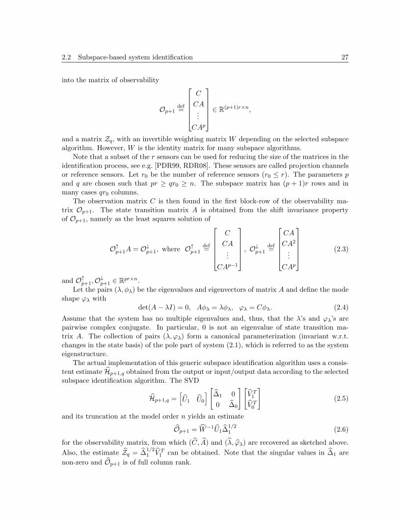
into the matrix of observability
Op+1def=
C
CA...
CAp
∈ R(p+1)r×n,
and a matrix Zq, with an invertible weighting matrix W depending on the selected subspacealgorithm. However, W is the identity matrix for many subspace algorithms.
Note that a subset of the r sensors can be used for reducing the size of the matrices in theidentification process, see e.g. [PDR99, RDR08]. These sensors are called projection channelsor reference sensors. Let r0 be the number of reference sensors (r0 ≤ r). The parameters pand q are chosen such that pr ≥ qr0 ≥ n. The subspace matrix has (p + 1)r rows and inmany cases qr0 columns.
The observation matrix C is then found in the first block-row of the observability ma-trix Op+1. The state transition matrix A is obtained from the shift invariance propertyof Op+1, namely as the least squares solution of
O↑p+1A = O↓p+1, where O↑p+1def=
C
CA...
CAp−1
, O↓p+1
def=
CA
CA2
...
CAp
(2.3)
and O↑p+1,O↓p+1 ∈ Rpr×n.Let the pairs (λ, φλ) be the eigenvalues and eigenvectors of matrix A and define the mode
shape ϕλ withdet(A− λI) = 0, Aφλ = λφλ, ϕλ = Cφλ. (2.4)
Assume that the system has no multiple eigenvalues and, thus, that the λ’s and ϕλ’s arepairwise complex conjugate. In particular, 0 is not an eigenvalue of state transition ma-trix A. The collection of pairs (λ, ϕλ) form a canonical parameterization (invariant w.r.t.changes in the state basis) of the pole part of system (2.1), which is referred to as the systemeigenstructure.
The actual implementation of this generic subspace identification algorithm uses a consis-tent estimate Hp+1,q obtained from the output or input/output data according to the selectedsubspace identification algorithm. The SVD
Hp+1,q =[U1 U0
] [∆1 0
0 ∆0
][V T1
V T0
](2.5)
and its truncation at the model order n yields an estimate
Op+1 = W−1U1∆1/21 (2.6)
for the observability matrix, from which (C, A) and (λ, ϕλ) are recovered as sketched above.
Also, the estimate Zq = ∆1/21 V T
1 can be obtained. Note that the singular values in ∆1 are
non-zero and Op+1 is of full column rank.
28 Chapter 2
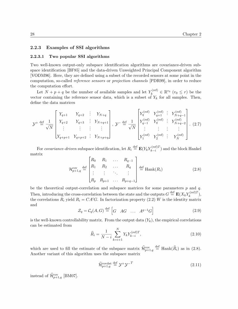
2.2.3 Examples of SSI algorithms
2.2.3.1 Two popular SSI algorithms
Two well-known output-only subspace identification algorithms are covariance-driven sub-space identification [BF85] and the data-driven Unweighted Principal Component algorithm[VODM96]. Here, they are defined using a subset of the recorded sensors at some point in thecomputation, so-called reference sensors or projection channels [PDR99], in order to reducethe computation effort.
Let N + p + q be the number of available samples and let Y(ref)k ∈ Rr0 (r0 ≤ r) be the
vector containing the reference sensor data, which is a subset of Yk for all samples. Then,define the data matrices
Y+ def=
1√N
Yq+1 Yq+2... YN+q
Yq+2 Yq+3... YN+q+1
......
......
Yq+p+1 Yq+p+2... YN+p+q
, Y− def
=1√N
Y(ref)q Y
(ref)q+1
... Y(ref)N+q−1
Y(ref)q−1 Y
(ref)q
... Y(ref)N+q−2
......
......
Y(ref)1 Y
(ref)2
... Y(ref)N
. (2.7)
For covariance-driven subspace identification, let Ridef= E(YkY
(ref)Tk−i ) and the block Hankel
matrix
Hcovp+1,q
def=
R0 R1 . . . Rq−1
R1 R2 . . . Rq...
.... . .
...
Rp Rp+1 . . . Rp+q−1
def= Hank(Ri) (2.8)
be the theoretical output-correlation and subspace matrices for some parameters p and q.
Then, introducing the cross-correlation between the state and the outputs Gdef= E(XkY
(ref)Tk ),
the correlations Ri yield Ri = CAiG. In factorization property (2.2) W is the identity matrixand
Zq = Cq(A,G)def=[G AG . . . Aq−1G
](2.9)
is the well-known controllability matrix. From the output data (Yk), the empirical correlationscan be estimated from
Ri =1
N − iN∑
k=i+1
YkY(ref)Tk−i , (2.10)
which are used to fill the estimate of the subspace matrix Hcovp+1,q
def= Hank(Ri) as in (2.8).
Another variant of this algorithm uses the subspace matrix
Hcovdatp+1,q
def= Y+Y−T (2.11)
instead of Hcovp+1,q [BM07].
2.2 Subspace-based system identification 29
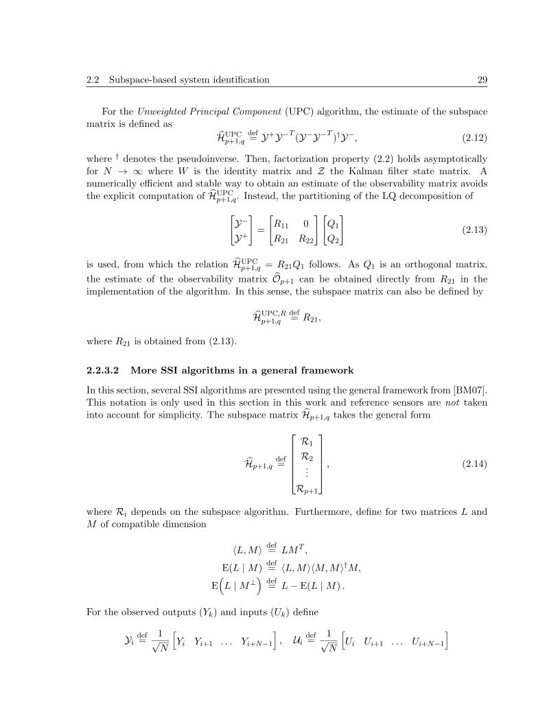
For the Unweighted Principal Component (UPC) algorithm, the estimate of the subspacematrix is defined as
HUPCp+1,q
def= Y+Y−T (Y−Y−T )†Y−, (2.12)
where † denotes the pseudoinverse. Then, factorization property (2.2) holds asymptoticallyfor N → ∞ where W is the identity matrix and Z the Kalman filter state matrix. Anumerically efficient and stable way to obtain an estimate of the observability matrix avoidsthe explicit computation of HUPC
p+1,q. Instead, the partitioning of the LQ decomposition of
[Y−Y+
]=
[R11 0
R21 R22
][Q1
Q2
](2.13)
is used, from which the relation HUPCp+1,q = R21Q1 follows. As Q1 is an orthogonal matrix,
the estimate of the observability matrix Op+1 can be obtained directly from R21 in theimplementation of the algorithm. In this sense, the subspace matrix can also be defined by
HUPC,Rp+1,q
def= R21,
where R21 is obtained from (2.13).
2.2.3.2 More SSI algorithms in a general framework
In this section, several SSI algorithms are presented using the general framework from [BM07].This notation is only used in this section in this work and reference sensors are not takeninto account for simplicity. The subspace matrix Hp+1,q takes the general form
Hp+1,qdef=
R1
R2...
Rp+1
, (2.14)
where Ri depends on the subspace algorithm. Furthermore, define for two matrices L andM of compatible dimension
〈L,M〉 def= LMT ,
E(L |M)def= 〈L,M〉〈M,M〉†M,
E(L |M⊥
)def= L− E(L |M) .
For the observed outputs (Yk) and inputs (Uk) define
Yi def=
1√N
[Yi Yi+1 . . . Yi+N−1
], Ui def
=1√N
[Ui Ui+1 . . . Ui+N−1
]

30 Chapter 2
and
Y+i,p+1
def=
Yi+1
Yi+2...
Yi+p+1
, Y−i,q
def=
YiYi−1
...
Yi−q+1
, U+
i,p+1def=
Ui+1
Ui+2...
Ui+p+1
, U−i,q
def=
UiUi−1
...
Ui−q+1
.
All subspace algorithms summarized in [BM07] can be segmented into two families, thealgorithms based on covariances
Ri def= 〈Yi, Z0〉
and the data-driven algorithms computing some conditional expectation
Ri def= E(Yi | Z0)
with some Z0 and the Ri plugged in (2.14). Both algorithms share the same formalism. Theycan be expressed in function of a single process Z0, also called instrument, the choice of thisinstrument being the determining factor in the design of the algorithm.
Output-only algorithms
Output-only covariance-driven subspace algorithm [BF85, POB+91], see also Equation(2.8)
Ri =[ri ri+1 · · · ri+q−1
]where rj = 〈Yj ,Y0〉
Basic output-only subspace algorithm [BM07], see also Equation (2.11)
Hp+1,q = 〈Y+0,p+1,Y−0,q〉
Output-only data-driven subspace algorithms [VODM96], see also Equation (2.12)
Hp+1,q = E(Y+0,p+1 | Y−0,q
)
In this form, it is called Unweighted Principal Component (UPC) in [VODM96]. Vari-ants of this algorithm use the subspace matrix W1Hp+1,qW2 with different weightingsW1 and W2:
– Principal Component (PC): W1 = I, W2 = Y−T0,q 〈Y−0,q,Y−0,q〉−1/2Y−0,q– Canonical Variate Algorithm (CVA): W1 = 〈Y+
0,p+1,Y+0,p+1〉−1/2, W2 = I

2.2 Subspace-based system identification 31
Input-Output algorithms (combined stochastic-deterministic)
Covariance-driven subspace algorithms using projected past input and output as instru-ments [VWO97]. They encompass the methods also known as IV, CVA, PO-MOESPand N4SID in their covariance form [VWO97]. For example, the instrumental variables(IV) method is defined by
Hp+1,q = 〈Y+0,p+1,L−0,q〉,
where L−0,q is obtained by stacking for i = −q + 1, . . . , 0
Lidef= E
(Wi
∣∣∣∣(U+0,p+1
)⊥), where Wi
def=
[Ui
Yi
]
Covariance-driven subspace algorithm with projection on the orthogonal of the input[GM03].
Ri =[ri ri+1 · · · ri+q−1
]where rj = 〈Yj ,Z0〉 and Z0
def= E
Y0
∣∣∣∣∣∣
[U+0,p+1
U−0,q
]⊥
(2.15)
Data-driven subspace algorithms with projection on the orthogonal of the input[VODM96]. This algorithm is known as the projection algorithm in [VODM96, Ch.2.3.2] and is computed from
Hp+1,q = E(Y+0,p+1 | Z−0,q
),
where Z−0,q is defined analogous to Y−0,q with corresponding Zi is as in (2.15).
Data-driven algorithms using projected inputs as instruments [Ver93, Ver94, CP04b].This algorithm was proposed by [Ver93, Ver94] under the name of PI-MOESP and wasrevisited in [CP04a, CP04b]. It results from the computation of
Hp+1,q = E(Y+0,p+1 | L−0,q
)
where L−0,q is defined by
Lidef= E
(Ui∣∣∣∣(U+0,p+1
)⊥), for i = −q + 1, . . . , 0.
Remark 2.1 (Subspace algorithms using frequency domain data) Many subspacemethods derived for time domain data have a frequency domain counterpart. Then, as pointedout in [BM07], frequency domain methods behave like their time-domain counterparts. LetL ∈ Ra,N and M ∈ Rb,N be matrices of compatible dimension and L ∈ Ra,N and M ∈ Rb,Ntheir Discrete Fourier Transform (DFT) with
L = LF, M = MF,
32 Chapter 2
where
Fdef=
1√N
e−2iπ0N . . . e−2iπ
0NN
e−2iπ1N . . . e−2iπ
1NN
......
...
e−2iπN−1N . . . e−2iπ
(N−1)NN
is the unitary Fourier matrix. Extending the definitions of 〈·, ·〉 and E(· | ·) to complex ma-trices leads to
〈L,M〉 = 〈L,M〉, E(L |M) = E(L |M)F.
Thus, the column space defined by these matrices is the same, either in frequency or intime domain, leading to the same system identification results. Frequency-domain subspacemethods are detailed for example in [MAL96, VODMDS97, Pin02, CGPV06, Akc10].
2.3 Statistical subspace-based fault detection
2.3.1 Context
The considered fault detection techniques are built on an asymptotically Gaussian residualfunction that compares a reference model with data. They date back to Benveniste et al. 1987[BBM87] and are based on Le Cam’s local approach [LC56]. A residual function associatedto subspace methods was proposed in [BAB00], on which this work is based. A summary ofthe local approach to change detection is found in [BBGM06].
With these methods, a χ2-test is performed on a residual function and compared toa threshold. Like this, it can be decided if the system is still in the reference state or ifthe system parameters have changed. The system parameterization is only needed in thereference state, while the residual function is computed directly from the data without theneed of knowing the system parameters in the tested state. An entirely non-parametricversion of the χ2-test was proposed in [BBB+08].
The subspace-based fault detection test finds especially application in vibration monitor-ing for the detection of structural damages (see also Section 2.4). It is extended to dam-age localization in [BMG04, BBM+08] by detecting changes of structural parameters. Asstructures are influenced by environmental conditions, especially temperature changes, therespective damage detection tests are also sensitive to these changes. Tests that are robust tothese changes are proposed in [BBB+08, BBMN09, BBM+10]. There are many applicationsof the subspace-based fault detection tests, see e.g. [MHVdA99, MGB03, MBG03, BBM+08,FK09, ZWM10].
2.3.2 The residual function and its statistical evaluation
Consider the model parameter θ of a system and its reference value θ0, which is for instanceidentified from data from the reference system. In this section, the model parameter isconsidered as a very general parameter, but it can already be viewed as a vector containinga canonical parameterization (eigenvalues, mode shapes) of a state-space system.

2.3 Statistical subspace-based fault detection 33
Consider a new data sample YTk,p+1,q = (Y Tk+p+1, . . . , Y
Tk+1, Y
Tk , . . . , Y
Tk−q+1), k = 1, . . . , N ,
of size N . The detection problem is to decide whether the new data – corresponding tosome parameter θ – are still well described by parameter θ0 or not. A primary residual func-tion K(θ′,Y) is introduced and some functions are derived that originate from this primaryresidual. They share the common notation:
For functions of two variables, the first variable corresponds to the model and the secondto the data.
Model parameter θ0 corresponds to a reference state, θ to an unknown state. Often,data corresponding to θ is confronted to the model defined by θ0.
When computing derivatives or expected values with respect to data, the first andsecond variable of these functions are denoted by θ′ and θ′′ to be unambiguous. At theend, θ0 or θ are plugged in.
2.3.2.1 Primary residual
The fundamental idea of the detection algorithm is to associate the model parameter θ0 witha vector-valued differentiable primary residual function K(θ′,Y), where the data Y are animplicit function of parameter θ′′, and dimK ≥ dim θ. This primary residual is constructedto satisfy the property [Bas98]
Eθ (K(θ0,Y)) = 0 iff θ = θ0, (2.16)
where Eθ is the expectation when the data Y correspond to the model parameter θ′′ = θ. Itsmean deviation with respect to the first variable is defined as
J (1)(θ0, θ)def= − ∂
∂θ′Eθ′′K
(θ′,Y
)∣∣∣∣θ′=θ0,θ′′=θ
. (2.17)
With respect to the second variable, the mean deviation is defined as
J (2)(θ0, θ)def=
∂
∂θ′′Eθ′′K
(θ′,Y
)∣∣∣∣θ′=θ0,θ′′=θ
. (2.18)
Both matrices J (1)(θ0, θ) and J (2)(θ0, θ) can be viewed as Jacobian matrices. Because of(2.16), both expressions are equivalent for θ = θ0 and the notation is simplified to
J (θ0)def= J (1)(θ0, θ0) = J (2)(θ0, θ0). (2.19)
The primary residual is linked to an estimation function [DB97, BBM87], as the modelparameter θ can theoretically be estimated from
θ = argθ′′
N∑
k=1
K(θ0,Yk,p+1,q) = 0
.

34 Chapter 2
2.3.2.2 Local approach to change detection
For a statistical evaluation of the residual its probability distribution is required, which isgenerally unknown for the function K. A solution to this problem is provided by Le Cam[LC56] with the concept of local asymptotic normality to compare statistical distributions by(an infinite number of) observations under close hypotheses. With this concept, the statisticallocal approach to change detection was developed [BBM87, BMP90, ZBB94, Bas98], whichis summarized now.
Assume the close hypotheses
H0 : θ = θ0
H1 : θ = θ0 + δθ/√N
(2.20)
where vector δθ is unknown but fixed. Note that for large N , hypotheses H1 corresponds tosmall deviations in θ. From the primary residual function K, define the residual function
ζN (θ0, θ)def=
1√N
N∑
k=1
K(θ0,Yk,p+1,q),
where the data Y corresponds to parameter θ. Define the residual covariance
ΣN (θ0, θ)def= Eθ
((ζN (θ0, θ)−EθζN (θ0, θ)) (ζN (θ0, θ)−EθζN (θ0, θ))
T), (2.21)
and its limitΣ(θ0)
def= lim
N→∞ΣN (θ0, θ). (2.22)
Note that it also holds
Σ(θ0) = limN→∞
ΣN (θ0, θ0) = limN→∞
Eθ0(ζN (θ0, θ0) ζN (θ0, θ0)T ) (2.23)
as θ → θ0 for N →∞ under the assumption of close hypotheses.Analogously to (2.17) and (2.18), define the Jacobians of the residual function as
J (1)N (θ0, θ)
def= − 1√
N
∂
∂θ′Eθ′′ζN (θ′, θ′′)
∣∣∣∣θ′=θ0,θ′′=θ
, (2.24)
J (2)N (θ0, θ)
def=
1√N
∂
∂θ′′Eθ′′ζN (θ′, θ′′)
∣∣∣∣θ′=θ0,θ′′=θ
. (2.25)
With (2.17)–(2.19) follows
J (1)(θ0, θ) = limN→∞
J (1)N (θ0, θ), J (2)(θ0, θ) = lim
N→∞J (2)N (θ0, θ) (2.26)
as well as
J (θ0) = limN→∞
J (1)N (θ0, θ) = lim
N→∞J (1)N (θ0, θ0) (2.27)
= limN→∞
J (2)N (θ0, θ) = lim
N→∞J (2)N (θ0, θ0) (2.28)

2.3 Statistical subspace-based fault detection 35
under the assumption of close hypotheses.
Under hypothesis H1, a small change in parameter θ, the expected value of the residualfunction with respect to data corresponding to (the unknown) parameter θ can be approx-imated by its Taylor expansion of first order, where (θ − θ0) is replaced by δθ/
√N . This
Taylor expansion can be made with respect to the first or with respect to the second variableof ζN (θ0, θ). In the first case, it holds
EθζN (θ0, θ) ≈ EθζN (θ, θ) +∂
∂θ′EθζN (θ′, θ)
∣∣∣∣θ′=θ
(θ0 − θ)
= − 1√N
∂
∂θ′EθζN (θ′, θ)
∣∣∣∣θ′=θ
δθ
= J (1)N (θ, θ)δθ, (2.29)
as EθζN (θ, θ) = 0 and using (2.24). In the second case, it holds
EθζN (θ0, θ) ≈ Eθ0ζN (θ0, θ0) +∂
∂θ′′Eθ′′ζN (θ0, θ
′′)
∣∣∣∣θ′′=θ0
(θ − θ0)
=1√N
∂
∂θ′′Eθ′′ζN (θ0, θ
′′)
∣∣∣∣θ′′=θ0
δθ
= J (2)N (θ0, θ0)δθ, (2.30)
as Eθ0ζN (θ0, θ0) = 0 and using (2.25). Thus, in both cases the mean of the residual functionasymptotically writes as J (θ0) δθ under the assumption of close hypotheses.
The residual function ζN (θ0, θ) is asymptotically Gaussian for a large class of primaryresiduals K and and the following Central Limit Theorem holds.
Theorem 2.2 Provided that Σ(θ0) is positive definite, the residual ζN (θ0, θ) is asymptoticallyGaussian distributed under both hypotheses H0 and H1 defined in (2.20) and it holds
ζN (θ0, θ)N−→
N (0,Σ(θ0)) under H0
N (J (θ0) δθ,Σ(θ0)) under H1
Hence, a change in the model parameter θ corresponds to a change of the mean of theasymptotically Gaussian distributed residual ζN (θ0, θ).
For simplicity of notation, we will use ζN (θ0) instead of ζN (θ0, θ) in the following, whilestill assuming that the data Y in the residual function corresponds to parameter θ.
2.3.2.3 Generalized likelihood ratio test
The generalized likelihood ratio test is a statistical test for making a decision between twohypotheses, where one hypothesis (the null hypothesis) is a special case of the other one. Con-sider the probability density functions pθ0 , pθ of a Gaussian random variable Z of dimension

36 Chapter 2
d with mean J δθ and covariance Σ under the hypotheses
H0 : δθ = 0
H1 : δθ 6= 0
The probability density function pθ writes as
pθ(Z) = (2π)−d2 (det(Σ))−
12 exp
−1
2(Z − J δθ)TΣ−1(Z − J δθ)
and the generalized log-likelihood ratio writes as
Υ(Z) = −2 logpθ0(Z)
supθ∈H1pθ(Z)
= ZTΣ−1Z + supθ∈H1
(−(Z − J δθ)TΣ−1(Z − J δθ)
)
= supθ∈H1
(2δθTJ TΣ−1Z − δθTJ TΣ−1J δθ
).
The supremum is reached at δθ? = (J TΣ−1J )−1J TΣ−1Z and it follows
Υ(Z) = ZTΣ−1J (J TΣ−1J )−1J TΣ−1Z.
Consider now the asymptotically Gaussian random variable ζN (θ0) and let J and Σ beconsistent estimates of its sensitivity (2.24) and covariance (2.22) computed from the referencemodel θ0. Then, the variable
χ2N (θ0)
def= Υ (ζN (θ0)) = ζN (θ0)
T Σ−1J (J T Σ−1J )−1J T Σ−1ζN (θ0)
is asymptotically χ2 distributed [LC86] with rank(J ) = dim(θ0) degrees of freedom, if J isfull column rank, and the non-centrality parameter δθT J T Σ−1J δθ under H1.
The decision between the hypotheses H0 and H1 is hence determined by the comparisonof χ2
N (θ0) to a threshold γ:
H0 : θ = θ0 if χ2N (θ0) < γ
H1 : θ = θ0 + δθ/√N if χ2
N (θ0) ≥ γ
2.3.3 Covariance-driven subspace-based residual and associated fault de-tection test
A residual function associated to covariance-driven subspace identification and the respectivefault detection test were derived by Basseville et al. [BAB00], which is summarized in thissection. The theoretical foundations of this algorithm are explained in the previous section.

2.3 Statistical subspace-based fault detection 37
2.3.3.1 Definition of residual and χ2-test
The model parameter θ ∈ C(r+1)n consists in the canonical parameterization of state-spacemodel (2.1) by the system eigenstructure
θdef=
[Λ
vec Φ
], where Λ
def=
λ1...
λn
, Φ
def=[ϕ1 . . . ϕn
](2.31)
with the eigenvalues λ1, . . . , λn and respective mode shapes ϕ1, . . . , ϕn of system (2.1), cf.(2.4).
The characterization of the model parameter θ by the estimation function (primary resid-ual) K(θ,Y) is based on the factorization Hp+1,q = Op+1Zq of the covariance-driven subspacematrix (2.8), where Hp+1,q ∈ R(p+1)r×qr0 . Write the observability matrix in the modal basis
Op+1(θ) =
Φ
Φ∆...
Φ∆p
∈ C(p+1)r×n, (2.32)
with the diagonal matrix ∆def= diag(Λ). Note that A = Ψ−1∆Ψ, where the columns of Ψ are
the eigenvectors of A, and Φ = CΨ.The following property characterizes whether a model parameter θ0 agrees with a subspace
matrix Hp+1,q:
Op+1(θ0) and Hp+1,q have the same left null space S.
From a model parameter θ0, the parametric observability matrix Op+1(θ) can be computed.The left null space S ∈ R(p+1)r×s can be obtained from an SVD of Op+1(θ) and it holds
STS = Is (2.33)
STOp+1(θ0) = 0, (2.34)
where s = (p + 1)r − n and n is the system order. Because the left null space S implicitlydepends on θ0, it is denoted by S(θ0), although it is not unique as S(θ0)W with an orthonor-mal matrix W is also a left null space. However, the particular choice of matrix W is notimportant, as will be seen in Section 2.3.3.5.
Hence, the characteristic property of the subspace matrix containing data in the referencestate θ = θ0 writes as
S(θ0)THp+1,q = 0.
To link this result with condition (2.16) for a primary residual K, the covariance-drivensubspace matrix is written as
Hp+1,q = E(Y+k,p+1Y−Tk,q
), (∀k), (2.35)
38 Chapter 2
where
Y+k,p+1
def=
Yk...
Yk+p
∈ R(p+1)r, Y−k,q
def=
Y(ref)k...
Y(ref)k−q+1
∈ Rqr0 .
With Z(Yk) = Y+k,p+1Y−Tk,q the primary residual K(θ0,Yk) ∈ Rsqr0 is defined as [BAB00]
K(θ0,Yk) def= vec
(S(θ0)
TZ(Yk)). (2.36)
Then, the estimate of the covariance-driven subspace matrix writes as
Hp+1,q =1
N
N∑
k=1
Z(Yk) (2.37)
and the subspace-based residual function ζN (θ0) ∈ Rsqr0 is defined as
ζN (θ0)def=
1√N
N∑
k=1
K(θ0,Yk) =√N vec
(S(θ0)
T Hp+1,q
). (2.38)
Note that for consistency of notation to [BAB97, BAB00, BMG04], the subspace-based resid-ual function is denoted as ζN (θ0) instead of ζN (θ0, θ) and the dependence on parameter θ,to which the data in Hp+1,q correspond, is implicit. The main properties of ζN (θ0) aresummarized in the following theorem, based on Sections 2.3.2.2 and 2.3.2.3.
Theorem 2.3 ([BAB00]) Assume the close hypotheses
H0 : θ = θ0
H1 : θ = θ0 + δθ/√N
where vector δθ ∈ C(r+1)n is unknown but fixed. Then, the residual function ζN (θ0) in (2.38)is asymptotically Gaussian distributed under both hypotheses H0 and H1 and it holds
ζN (θ0)N−→
N (0,Σ(θ0)) under H0
N (J (θ0) δθ,Σ(θ0)) under H1
where J (θ0) ∈ Csqr0×(r+1)n and Σ(θ0) ∈ Rsqr0×sqr0 are the sensitivity and covariance of theresidual function. Hypothesis H0 can be tested against H1 by comparing the variable
χ2N (θ0) = ζN (θ0)
T Σ−1J (J T Σ−1J )−1J T Σ−1ζN (θ0) (2.39)
with a threshold, where J and Σ are consistent estimates of J (θ0) and Σ(θ0). The variableχ2N (θ0) is asymptotically χ2 distributed with rank(J ) = dim(θ0) = (r+1)n degrees of freedom,
if J is full column rank, and the non-centrality parameter δθT J T Σ−1J δθ under H1.
To evaluate the χ2-test statistics (2.39), estimates J and Σ of the residual’s asymptoticsensitivity and covariance J (θ0) and Σ(θ0) are needed. Note that neither the residual’s
sensitivity J (1)N (θ0, θ) or J (2)
N (θ0, θ), nor its covariance ΣN (θ0, θ) are considered here, as theyconverge to J (θ0) and Σ(θ0), respectively (cf. Equations (2.21)–(2.30)). Thus, they can becomputed in the reference state θ0 and are detailed in the following sections.
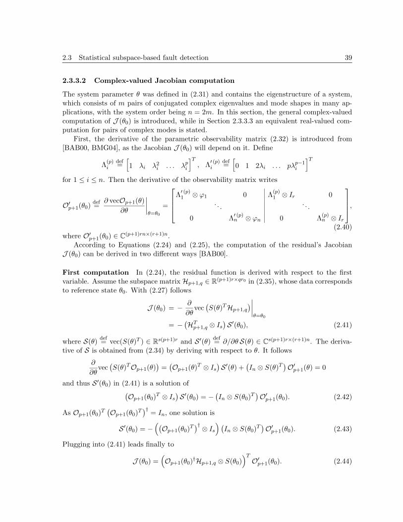
2.3 Statistical subspace-based fault detection 39
2.3.3.2 Complex-valued Jacobian computation
The system parameter θ was defined in (2.31) and contains the eigenstructure of a system,which consists of m pairs of conjugated complex eigenvalues and mode shapes in many ap-plications, with the system order being n = 2m. In this section, the general complex-valuedcomputation of J (θ0) is introduced, while in Section 2.3.3.3 an equivalent real-valued com-putation for pairs of complex modes is stated.
First, the derivative of the parametric observability matrix (2.32) is introduced from[BAB00, BMG04], as the Jacobian J (θ0) will depend on it. Define
Λ(p)i
def=[1 λi λ2i . . . λpi
]T, Λ
′ (p)i
def=[0 1 2λi . . . pλp−1i
]T
for 1 ≤ i ≤ n. Then the derivative of the observability matrix writes
O′p+1(θ0)def=
∂ vecOp+1(θ)
∂θ
∣∣∣∣θ=θ0
=
Λ′ (p)1 ⊗ ϕ1 0 Λ
(p)1 ⊗ Ir 0
. . .. . .
0 Λ′ (p)n ⊗ ϕn 0 Λ
(p)n ⊗ Ir
,
(2.40)where O′p+1(θ0) ∈ C(p+1)rn×(r+1)n.
According to Equations (2.24) and (2.25), the computation of the residual’s JacobianJ (θ0) can be derived in two different ways [BAB00].
First computation In (2.24), the residual function is derived with respect to the firstvariable. Assume the subspace matrix Hp+1,q ∈ R(p+1)r×qr0 in (2.35), whose data correspondsto reference state θ0. With (2.27) follows
J (θ0) = − ∂
∂θvec(S(θ)THp+1,q
)∣∣∣∣θ=θ0
= −(HTp+1,q ⊗ Is
)S ′(θ0), (2.41)
where S(θ)def= vec(S(θ)T ) ∈ Rs(p+1)r and S ′(θ) def
= ∂/∂θ S(θ) ∈ Cs(p+1)r×(r+1)n. The deriva-tive of S is obtained from (2.34) by deriving with respect to θ. It follows
∂
∂θvec(S(θ)TOp+1(θ)
)=(Op+1(θ)
T ⊗ Is)S ′(θ) +
(In ⊗ S(θ)T
)O′p+1(θ) = 0
and thus S ′(θ0) in (2.41) is a solution of(Op+1(θ0)
T ⊗ Is)S ′(θ0) = −
(In ⊗ S(θ0)
T)O′p+1(θ0). (2.42)
As Op+1(θ0)T(Op+1(θ0)
T)†
= In, one solution is
S ′(θ0) = −((Op+1(θ0)
T)† ⊗ Is
) (In ⊗ S(θ0)
T)O′p+1(θ0). (2.43)
Plugging into (2.41) leads finally to
J (θ0) =(Op+1(θ0)
†Hp+1,q ⊗ S(θ0))TO′p+1(θ0). (2.44)

40 Chapter 2
Second computation In (2.25) the residual function is derived with respect to the secondvariable. With (2.28) follows
J (θ0) =∂
∂θvec(S(θ0)
THp+1,q
)∣∣∣∣θ=θ0
,
where Hp+1,q is an implicit function of θ. From (2.2) follows Hp+1,q = Op+1(θ)Zq and thus
J (θ0) =(ZTq ⊗ S(θ0)
T)O′p+1(θ0).
Then, Zq = Op+1(θ0)†Hp+1,q and
J (θ0) =(Op+1(θ0)
†Hp+1,q ⊗ S(θ0))TO′p+1(θ0). (2.45)
Note that in both computations, J (θ0) does not depend on the particular scaling ofthe mode shapes in θ0: Scaling the mode shapes ϕ1, . . . , ϕn with some constants α1, . . . , αnleads to the parametric observability matrix Op+1(θ0)D, where D = diag(α1, . . . , αn). Itsderivative in (2.40) then writes as (D ⊗ I(p+1)r)O′p+1(θ0) and hence
J (θ0) =(
(Op+1(θ0)D)†Hp+1,q ⊗ S(θ0))T
(D ⊗ I(p+1)r)O′p+1(θ0)
=(D−1 (Op+1(θ0))
†Hp+1,q ⊗ I(p+1)rS(θ0))T
(D ⊗ I(p+1)r)O′p+1(θ0)
=(Op+1(θ0)
†Hp+1,q ⊗ S(θ0))TO′p+1(θ0).
In both computations, a consistent estimate J of J (θ0) is obtained by replacing Hp+1,q
in (2.44) or (2.45) with an estimate Hp+1,q (cf. (2.37)) that is obtained from a data samplefrom the reference state corresponding to θ0.
2.3.3.3 Real-valued Jacobian computation
If the system parameter θ consists of m pairs of conjugated complex eigenvalues and modeshapes, with the system order being n = 2m, the computation of the Jacobian J (θ0) can bedone in real values [BAB97, BMG04]. This is for example the case for structural vibrationanalysis, see also Section 2.4.
Recall the definition of θ from (2.31):
θ =
[Λ
vec Φ
], where Λ
def=
λ1...
λn
, Φ
def=[ϕ1 . . . ϕn
]
Let Λc ∈ Cm and Φc ∈ Cr×m contain one element of each pair of the conjugated complexeigenvalues and mode shapes, respectively, such that
Λ =
[Λc
Λc
], Φ =
[Φc Φc
]

2.3 Statistical subspace-based fault detection 41
and thus
θ =
Λc
Λc
vec Φc
vec Φc
.
Define analogously
θcdef=
[Λc
vec Φc
]∈ C(r+1)m.
Then, the parametric observability matrix (2.32) writes as
Op+1(θ) =
Φc Φc
Φc∆c Φc∆c...
...
Φc∆pc Φc∆
pc
=[Op+1(θc) Op+1(θc)
],
where ∆c = diag(Λc). Now define the real-valued system parameter θ by
θdef=
[<(θc)
=(θc)
]=
<(Λc)
vec<(Φc)
=(Λc)
vec=(Φc)
∈ R(r+1)2m (2.46)
and its corresponding real-valued parametric observability matrix by
Op+1(θ)def=
<(Φc) =(Φc)
<(Φc∆c) =(Φc∆c)...
...
<(Φc∆pc) =(Φc∆
pc)
=[< (Op+1(θc)) = (Op+1(θc))
]∈ R(p+1)r×2m. (2.47)
Then, the relation
Op+1(θ) = Op+1(θ)T
holds with the invertible matrix
T =1
2
[Im −iIm
Im iIm
],
where (√
2T )(√
2T )∗ = I. Thus, the left null space S(θ0) of Op+1(θ0) with the properties(2.33)–(2.34) is equivalent to a left null space S(θ0) of Op+1(θ0). Hence, the left null spaceS(θ0) can be replaced by S(θ0) in the residual computation and the system parameter θ0 canbe used instead of θ0.

42 Chapter 2
Note that in the modal basis defined by Op+1(θ), the state transition and observationmatrices write as
A = T−1∆T =
[<(∆c) =(∆c)
−=(∆c) <(∆c)
], C = ΦT =
[<(Φc) =(Φc)
].
For the Jacobian computation using the real-valued system parameter θ, the derivative
O′p+1(θ0)def=
∂ vecOp+1(θ)
∂θ
∣∣∣∣∣θ=θ0
of the real-valued observability matrix is needed, where O′p+1(θ0) ∈ R(p+1)r2m×(r+1)2m. With(2.46)–(2.47) it holds
O′p+1(θ) =
∂ vec< (Op+1(θc))
∂<(θc)
∂ vec< (Op+1(θc))
∂=(θc)
∂ vec= (Op+1(θc))
∂<(θc)
∂ vec= (Op+1(θc))
∂=(θc)
. (2.48)
In (2.40), the complex-valued derivative O′p+1(θ0) ∈ C(p+1)r2m×(r+1)2m was defined. The
complex-valued derivative O′p+1(θc) ∈ C(p+1)rm×(r+1)m with respect to parameter θc can bedefined analogously. With the Wirtinger derivatives [Fis05] of a complex-valued function itfollows
O′p+1(θc) =∂ vec< (Op+1(θc))
∂θc+ i
∂ vec= (Op+1(θc))
∂θc
=1
2
(∂ vec< (Op+1(θc))
∂<(θc)− i
∂ vec< (Op+1(θc))
∂=(θc)+ i
∂ vec= (Op+1(θc))
∂<(θc)
+∂ vec= (Op+1(θc))
∂=(θc)
).
Then, the elements of matrix O′p+1(θ) in (2.48) are obtained from O′p+1(θc) by using the
Cauchy-Riemann equations1
∂ vec< (Op+1(θc))
∂<(θc)=∂ vec= (Op+1(θc))
∂=(θc),
∂ vec< (Op+1(θc))
∂=(θc)= −∂ vec= (Op+1(θc))
∂<(θc)
and it follows
O′p+1(θ) =
<(O′p+1(θc)) −=(O′p+1(θc))
=(O′p+1(θc)) <(O′p+1(θc))
. (2.49)
Thus, the real-valued computation of the Jacobian J (θ0) analogous to (2.44) and (2.45)writes
J (θ0) =(Op+1(θ0)
†Hp+1,q ⊗ S(θ0))TO′p+1(θ0), (2.50)
1Op+1(θc) is a polynomial function and thus holomorphic. Hence the Cauchy-Riemann equations aresatisfied.

2.3 Statistical subspace-based fault detection 43
where the real-valued observability matrix Op+1(θ0) is computed in (2.47), the left null spaceS(θ0) is computed on Op+1(θ0) and O′p+1(θ0) is obtained from (2.49) at θ = θ0.
A consistent estimate J of J (θ0) is obtained by replacingHp+1,q in (2.50) with an estimate
Hp+1,q that is obtained from a data sample from the reference state corresponding to θ0. Notethat θ0 and θ0 denote equivalent canonical parameterizations of the system in the referencestate, where the former is complex-valued and the latter real-valued.
2.3.3.4 Covariance computation
The covariance of the residual function in the reference state is defined in (2.22) and obtainedusing data in the reference state in (2.23):
Σ(θ0) = limN→∞
Eθ0(ζN (θ0) ζN (θ0)T ) ∈ Rsqr0×sqr0
A consistent estimate Σ of the covariance is obtained from the empirical covariance of a sample
of residuals ζ(k)Nb
(θ0), k = 1, . . . , nb, that are computed on different, statistically independentparts of the data, where nb is the number of data samples that are each of length Nb. Let Nbe fixed, and let the nb independent data samples be chosen such that N = nbNb. Denotethe estimates (2.37) of the covariance-driven subspace matrix on each data sample of length
Nb with H(k)p+1,q and the estimate on the data sample of length N with Hp+1,q. Then,
limN→∞
Hp+1,q = limN→∞
1
nb
nb∑
k=1
H(k)p+1,q.
and thus, the covariance of ζN can be expressed as the covariance of the ζ(k)Nb
:
Σ = cov(ζN (θ0)) = cov(ζ(k)Nb
(θ0)).
Replacing the latter with the sample covariance, where the mean Eθ0ζ(k)Nb
(θ0) = 0 is known,yields the estimate
Σ =1
nb
nb∑
k=1
ζ(k)Nb
(θ0)ζ(k)Nb
(θ0)T .
2.3.3.5 Invariance property of χ2-test
The χ2-test (2.39) possesses some important invariance properties.
Lemma 2.4 ([BAB97, Bas99, BAB00]) The χ2-test (2.39) is unchanged when the pri-mary residual function K in (2.36) is premultiplied by an invertible matrix T .
Proof: For the primary residual TK, the subspace-based residual function writesTζN (θ0) and consistent estimates of its sensitivity and covariance are T J and T ΣT T , when
44 Chapter 2
J and Σ are consistent estimates of the sensitivity and covariance of ζN (θ0). Then,
χ2N (θ0) = (TζN (θ0))
T (T ΣT T )−1(T J )(
(T J )T (T ΣT T )−1(T J ))−1
(T J )T (T ΣT T )−1TζN (θ0)
= ζN (θ0)T Σ−1J (J T Σ−1J )−1J T Σ−1ζN (θ0).
In the definition of the left null space S(θ0) in Section 2.3.3.1, the matrix S(θ0) can bereplaced by S(θ0)W , where W is an orthogonal matrix. This leads to a residual function
ζN,W (θ0) =√N vec
((S(θ0)W )T Hp+1,q
)= (I ⊗W T )ζN (θ0).
Thus, from Lemma 2.4 follows that the choice of W has no effect on the resulting χ2-teststatistics. Further aspects of the invariance property are considered in Section 3.4.2.
2.3.4 Non-parametric versions of the covariance-driven subspace-basedfault detection test
This section addresses two implementations of the fault detection test that have provenefficient in practice and were shown in [BBB+08]. They use an entirely non-parametricversion of the test, where no system parameter θ0 needs to be known in the reference state.With this strategy, a test is proposed where an empirical null space S is used, which is the nullspace of different reference states. This can be used for a test that is robust to environmentalchanges. Applications of the non-parametric test are found e.g. in [FM02, YG06, SBMT08,FK09, SMR+09].
2.3.4.1 Non-parametric test
In some cases, it is of interest to replace the parametric approach with a non-parametricone, based on an empirical null space S computed on a reference data set and not on theparametric observability matrix (2.32) or (2.47). Such a null space may result from a SVDof the empirical subspace matrix built on the reference data set (here indexed with 0) and itholds
ST S = Is,
ST H (0)p+1,q = 0 (2.51)
instead of (2.33)–(2.34). The subspace matrix H (0)p+1,q corresponds to reference parameter
θ0 in the previous sections, which is not needed to be known in this case. While θ0 wouldbe estimated from data in practice and thus contains only limited information about the
system in the reference state, the computation of S directly on H (0)p+1,q uses the entire system
response.
2.4 Structural vibration analysis 45
Based on a new data set of length N from the (possibly faulty) system, the empiricalsubspace matrix Hp+1,q (corresponding to state θ) is computed and the residual then writes
ζNdef=√N vec
(ST Hp+1,q
).
As there is no system parameterization, no sensitivity matrix needs to be taken care of. Theχ2-test statistics (2.39) boils down to
χ2N
def= ζTN Σ−1ζN , (2.52)
where Σ is an estimate of the covariance of ζN , which can be computed analogous to Section2.3.3.4.
Note that the empirical χ2-test statistics (2.52) corresponds to testing hypotheses H0
against H1 in Theorem 2.3, where J (θ0) = I. Thus, the residual function plays the role ofthe underlying system parameter itself.
2.3.4.2 Merging different reference states
Assume that J reference data sets are available with corresponding subspace matrices
H (0,1)p+1,q, . . . , H
(0,J)p+1,q that relate to (slightly) different system parameters θ0,1, . . . , θ0,J . This
happens e.g. in structural vibration analysis, where the modal parameters of the healthystructure vary under different environmental conditions. A left null space S is desired withthe property
ST H (0,k)p+1,q = 0, k = 1, . . . , J.
An empirical solution to this problem was proposed in [BBB+08] by the computation of S
on the average of the subspace matrices H (k)p+1,q, such that
STJ∑
k=1
H (0,k)p+1,q = 0.
Then, the residual covariance Σ is computed using the subspace matrices H (0,k)p+1,q, k = 1, . . . , J .
The corresponding χ2-test statistics (2.52) then reacts on changes in the system from thestates corresponding to θ0,1, . . . , θ0,J , but not from a change in the system between thereference states corresponding to some θ0,i to θ0,j . This approach was validated e.g. in[BBM+06, RMLDR08, AMR09, SMR+09].
2.4 Structural vibration analysis
An important application of subspace-based system identification and fault detection lies inthe field of vibration analysis of mechanical, civil and aeronautical structures. In this section,the underlying mechanical model is introduced and its relation to the state space model (2.1)is shown [POB+91, Jua94, PDR99]. Also, practical issues for the modal analysis of structuresare considered.

46 Chapter 2
2.4.1 Modeling and eigenstructure identification
The behavior of a mechanical structure is described by a continuous-time, time-invariant,linear dynamical system, modeled by the vector differential system
M X (t) + C1X (t) +KX (t) = υ(t)
Y (t) = LX (t)(2.53)
where t denotes continuous time; M , C1, and K are mass, damping, and stiffness matrices,respectively; the (high dimensional) state vector X (t) is the displacement vector of the degreesof freedom of the structure; the external unmeasured force υ is modeled as stationary whitenoise with covariance matrix Qυ(t); measurements are collected in the (low dimensional)vector Y and matrix L indicates which degrees of freedom are actually measured, i.e. thesensor locations.
The matrices (M,C1,K) cannot be recovered from measured outputs. However, theparameters to be identified are the eigenvalues (or modes) µ and mode shapes ψµ of system(2.53), which comprise the modal parameters and are solutions of
(µ2M + µC1 +K)Ψµ = 0, ψµ = LΨµ. (2.54)
Sampling model (2.53) at rate 1/τ yields the discrete time state space model (2.1), where thestate and the output are
Xk =
[X (kτ)
X (kτ)
], Yk = Y (kτ),
the state transition and observation matrices are
A = eLτ , where L =
[0 I
−M−1K −M−1C1
], C =
[L 0
].
The state noise (Vk) is stationary, zero-mean, white, with covariance
Qdef= E
(Vk V
Tk
)=
∫ (k+1)τ
kτeLs Q(s) eL
T sds, where Q(s) =
[0 0
0 M−1Qυ(s)M−1
].
The eigenstructure (λ, ϕλ) of system (2.1) is defined by the eigenvalues and eigenvectors ofA and by C:
(A− λI)φλ = 0, ϕλ = Cφλ. (2.55)
The desired modal parameters in (2.54) are equivalently found in the eigenstructure (λ, ϕλ)of (2.1) and it holds
eµτ = λ, ψµ = ϕλ.
The modal frequencies f and damping coefficients ρ are recovered directly from the eigenval-ues λ by
f =a
2πτ, ρ =
100|b|√a2 + b2
, (2.56)
2.4 Structural vibration analysis 47
where a = | arctan<(λ)/=(λ)| and b = ln |λ|.Thus, vibration analysis is stated as the problem of identifying the eigenstructure of a
linear dynamic system. Parameters of interest are modes (modal frequencies f , dampingratios ρ) and mode shapes ϕλ.
2.4.2 Further modeling issues
2.4.2.1 Sensor types
The measurement equation in (2.53) assumes that the sensors are displacement sensors suchas strain gauges. If strain gauges, velocity sensors or accelerometers are available, the mea-surement equation in (2.53) can be written as
Y (t) =
L1X (t)
L2X (t)
L3X (t)
,
and the corresponding discrete time system (2.1) holds with
C =
L1 0
0 L2
−L3M−1K −L3M
−1C1
.
Consequently, the state-space model (2.1) is valid for those three types of sensors and thenature of the sensors influences the observation matrix C only. When accelerometers areused, the sensor noise and process noise are correlated, although we ignore this effect.
2.4.2.2 Input excitation
In Section 2.4.1, the unknown excitation force υ(t) is assumed to be stationary Gaussianwhite noise for simplicity. However, it is more realistic to assume a non-stationary excitation.This is no shortcoming for the subspace algorithms, as non-stationary consistency of manysubspace algorithms for eigenstructure identification was shown in [BM07].
Also, the whiteness assumption made on the input force υ(t) seems unrealistic. Theunknown excitation forces are typically a superposition of harmonics due to rotating partsas well as colored ambient excitation noise. When processing the measured responses withsubspace-based algorithms, harmonics due to rotating parts are found in the form of poleswith zero damping. Since the frequency of rotation is usually known, those harmonics canbe discarded from the results of the analysis. On the other hand, colored input excitationcan always be represented as the output of an unknown excitation filter driven by whitenoise [GD91, BBGM07]. In this case, (2.53) represents the combined system including theexcitation filter. Therefore, (2.54) collects the modes and mode shapes of the combinedsystem. Since the poles corresponding to the excitation filter are generally highly damped,these poles can easily be separated from structural modes, which typically have a much lowerdamping coefficient.

48 Chapter 2
2.4.2.3 Measurement noise
Measurement noise was neither considered in model (2.1) nor in model (2.53). This is some-what unrealistic and the measurement equation in model (2.1) should rather be
Yk = CXk + εk,
where εk is a Gaussian, zero mean, moving-average sequence. However, this kind of noisecan be encompassed up to an index shift when filling the subspace matrix for the subspacealgorithm [VODM96, BAB00]. With this assumption on εk, the measurement noise doesnot affect the eigenstructure of the system in (2.1). This property does not hold if εk is anautoregressive sequence.
2.4.3 The stabilization diagram
In Operational Modal Analysis (OMA), the eigenstructure of mechanical, civil and aeronau-tical structures is identified from output-only data under ambient excitation. With forcedexcitation e.g. by shakers (exogenous inputs, OMAX), some of the inputs are available. Inboth cases, the selection of the model order in (2.5), and thus the parameters p and q of thesubspace matrix Hp+1,q on one hand, and the handling of excitation and measurement noiseson the other hand, are two major practical issues.
In order to retrieve a desired number of modes, an even larger model order must beassumed while performing identification. A number of spurious modes appear in the iden-tified model due to this over-specification, as well as due to colored noise or non-linearities.Techniques from statistics to estimate the best model order, such as AIC, BIC or MDL[Aka74a, Ris78, CMK01], or model order estimation techniques specifically for subspacemethods as in [Bau01] may lead to a model with the best prediction capacity. How-ever, one is rather interested in a model containing only the physical modes of the inves-tigated structured, while rejecting the spurious modes. Based on the observation that phys-ical modes remain quite constant when estimated at different over-specified model orders,while spurious modes vary, they can be distinguished using so-called stabilization diagrams[PDR99, PDR01, VdAP04, CGV+05, Bak11]. There, frequencies estimated from multi-ordersystem identification are plotted against the model order. From the modes common to manymodels and using further stabilization criteria, such as a threshold on damping values, lowvariation between modes and mode shapes of successive orders etc., the final estimated modelis obtained.
Chapter 3
Some numerical considerations forsubspace-based algorithms
3.1 Introduction
This chapter has the purpose to introduce and derive some numerical tools, which are neededthroughout this work. Furthermore, theoretical properties and practical issues concerningthe fault detection test of Section 2.3.3 are derived.
In Section 3.2, definitions of the QR, LQ and singular value decompositions are stated,as well as properties of the vectorization operator and the Kronecker product.
In Section 3.3, an iterative least squares solution for strongly over-determined systems ofequations using the QR decomposition is derived. This algorithm will be useful in Chapters 4and 5 for an iterative solution of the least squares problem for the state transition matrix.Furthermore, an efficient computation of sensitivities of the singular vectors of a randommatrix is derived in the same section, which will be useful in Chapter 6 for the covariancecomputation of a fault detection residual based on the left singular vectors.
In Section 3.4, additional properties of the statistical subspace-based fault detection testof Section 2.3.3 are derived and clarified. They are mainly of theoretical value and concernthe computation of the asymptotic Jacobian of the residual as well as an invariance propertyof the associated χ2-test. The latter concerns the selected null space and weightings for thesubspace matrix. For these issues, inconsistent statements have been made in literature andthis section helps to clarify them.
In Section 3.5, some practical issues of the fault detection test are addressed, whichare important for the implementation of the algorithm and its application to real data. Inmany cases, the estimate of the residual’s asymptotic covariance matrix is rank deficientdue to a lack of data. For this case, a numerically robust and efficient computation of theassociated χ2-test is proposed. Furthermore, the computation of the covariance estimate

50 Chapter 3
itself is explained in detail for covariance-driven SSI and extended to data-driven SSI withthe UPC algorithm. These computations are applied for damage detection using ambientvibration data of a bridge in Chapter 9.
Note that Sections 3.3–3.5 can be skipped for a first reading.
3.2 Definitions
3.2.1 QR decomposition and Singular Value Decomposition
In this section, the notation for QR, LQ and singular value decompositions is defined, basedon [GVL96].
Definition 3.1 The QR decomposition of a matrix Z ∈ Ra×b is denoted by
Z = Q1R1,
where Q1 ∈ Ra×a is an orthogonal matrix with QT1Q1 = Q1QT1 = I and R1 ∈ Ra×b is an
upper triangular matrix. For a ≥ b the thin QR decomposition is denoted by
Z = Q2R2,
where Q2 ∈ Ra×b is a matrix with orthonormal columns (QT2Q2 = I) and R2 ∈ Rb×b is anupper triangular matrix.
Analogously, the LQ decomposition of a matrix Z ∈ Ra×b is denoted by
Z = R3Q3,
where R3 ∈ Ra×b is a lower triangular matrix and Q3 ∈ Rb×b is an orthogonal matrix withQT3Q3 = Q3Q
T3 = I. For a ≤ b the thin LQ decomposition is denoted by
Z = R4Q4,
where R4 ∈ Ra×a is a lower triangular matrix and Q4 ∈ Ra×b is a matrix with orthonormalrows (Q4Q
T4 = I).
Note that if Z is full column rank, R2 from the thin QR decomposition is invertible. IfZ is full row rank, R4 from the thin LQ decomposition is invertible. Still, in both cases, thethin decompositions are not unique. However, they can be defined in a unique way, e.g. bypositive values on the diagonal of R2 and R4, respectively.
In this work, mainly the thin QR and thin LQ decompositions are used.
Definition 3.2 The singular value decomposition (SVD) of a matrix Z ∈ Ra×b is denotedby
Z = U∆V T

3.2 Definitions 51
where U ∈ Ra×a and V ∈ Rb×b are orthogonal matrices containing the left and right singularvectors, and
∆ =
[∆ 0
], if a < b,[
∆
0
], if a > b,
∆, if a = b,
where ∆ = diag(σ1, . . . , σmina,b) is the diagonal matrix containing the singular values of Zwith σ1 ≥ . . . ≥ σmina,b.
For a > b the thin SVD of Z is defined by
Z = U1∆VT ,
where U1 ∈ Ra×b is the first block of the partitioned matrix U =[U1 U2
].
Note that again, the thin SVD of a matrix Z is not a unique decomposition, even if Zis full column rank. However, it can be defined uniquely, e.g. by positive values of the firstcomponent of each left singular vector as in the following definition.
Definition 3.3 Let Z = U∆V T be an arbitrary SVD of matrix Z, where
U =[u1 . . . un
], V =
[v1 . . . vn
]
and n = rank(Z). For j = 1, . . . , n define
uj = sign(u1,j)u1,j , vj = sign(u1,j)v1,j ,
where u1,j is the first entry of vector uj, and
U =[u1 . . . un
], V =
[v1 . . . vn
].
Then, U∆V T is called unique SVD of Z.
In this work, the full SVD is used for the computation of left null spaces. In all othercases, the thin SVD is used.
3.2.2 Vectorization operator and Kronecker product
In this work, the vectorization operator
vecG =
g1
g2...
gn
for G =[g1 g2 . . . gn
]∈ Rm×n

52 Chapter 3
is used extensively. Here, some properties related to Kronecker products are recalled andformulas for vecGT are derived. They are stated in [Fac05, Bro11] and proved in the following.
For arbitrary matrices A ∈ Rp×m, B ∈ Rn×q the Kronecker product A ⊗ B ∈ Rnp×mq isdefined as
A⊗B =
a11B a12B . . . a1mB
a21B a22B . . . a2mB...
.... . .
...
ap1B ap2B . . . apmB
, where A =
a11 a12 . . . a1m
a21 a22 . . . a2m...
.... . .
...
ap1 ap2 . . . apm
.
An important property of the vectorization operation is
vec(AGB) = (BT ⊗A)vecG. (3.1)
Definition 3.4 For i ∈ 1, . . . , n define the unit vector
e(n)i
def=[0 . . . 0 1 0 . . . 0
]T∈ Rn,
where the entry 1 is at the i-th position. Then, the permutation matrix Pm,n ∈ Rmn×mn isdefined as
Pm,n def=
e(n)1 ⊗ e(m)T
1 e(n)2 ⊗ e(m)T
1 . . . e(n)n ⊗ e(m)T
1
e(n)1 ⊗ e(m)T
2 e(n)2 ⊗ e(m)T
2 . . . e(n)n ⊗ e(m)T
2...
.... . .
...
e(n)1 ⊗ e(m)T
m e(n)2 ⊗ e(m)T
m . . . e(n)n ⊗ e(m)T
m
=
In ⊗ e(m)T1
In ⊗ e(m)T2
...
In ⊗ e(m)Tm
.
Lemma 3.5 ([Fac05, Bro11]) Let A ∈ Rp×m, B ∈ Rn×q and G ∈ Rm×n. Then, thepermutation matrix Pm,n has the following properties:
(a) PTm,nPm,n = Pm,nPTm,n = Imn
(b) PTm,n = Pn,m
(c) Pm,nvecG = vecGT
(d) Pn,p(A⊗B)Pm,q = B ⊗A
Proof: Items (a) and (b) follow directly from the definition of Pm,n. To prove item (c),write the vectorization operation as
vecG =
Ge(n)1
Ge(n)2...
Ge(n)n
, vecGT =
GT e(m)1
GT e(m)2
...
GT e(m)m
. (3.2)
3.2 Definitions 53
Then, using Definition (3.4) the k-th block of the product Pm,nvecG writes
[Pm,nvecG
]k
def=[e(n)1 ⊗ e(m)T
k e(n)2 ⊗ e(m)T
k . . . e(n)n ⊗ e(m)T
k
]vecG
=n∑
i=1
(e(n)i ⊗ e
(m)Tk
)Ge
(n)i .
From Ge(n)i = vec(Ge
(n)i ) and with property (3.1) follows
[Pm,nvecG
]k
=n∑
i=1
vec(e(m)Tk
(Ge
(n)i
)e(n)Ti
)
= vec
(e(m)Tk G
n∑
i=1
e(n)i e
(n)Ti
)
= vec(e(m)Tk G
).
As(e(m)Tk G
)is a row vector, its transposed is vec
(e(m)Tk G
)and thus
[Pm,nvecG
]k
= GT e(m)k .
Comparing this result with the k-th block of vecGT in (3.2) proves (c).
The proof of (d) is stated from [Fac05]: Let C ∈ Rm×q be an arbitrary matrix. Then,with property (3.1) and (c) it follows
Pn,p(A⊗B)Pm,qvecC = Pn,p(A⊗B)vecCT
= Pn,pvec(BCTAT
)
= vec(ACBT
)
= (B ⊗A)vecC.
The fact that C is arbitrary finishes the proof.
Remark 3.6 The matrix Pm,n coincides with the matrix
P =
m∑
k1=1
n∑
k2=1
Em,nk1,k2⊗ En,mk2,k1
defined in [PGS07, RPDR08], where Em,nk1,k2∈ 0, 1m×n are matrices whose entries are zeros,
except the entry at position (k1, k2) which is one.

54 Chapter 3
3.3 Some numerical tools
3.3.1 Iterative QR decompositions
In some cases, thin QR decompositions of a large matrix G ∈ Rm,n with m n are necessary,where only matrix R is needed. With the following lemma, the QR decomposition of G isdone iteratively on blocks of G, while in each step only the R part needs to be saved in orderto obtain the corresponding R part of G.
Lemma 3.7 Let G0, . . . , GJ , where Gj ∈ Rmj×n for j = 0, . . . , J , be the J + 1 block rows ofa matrix
G =
G0...
GJ
∈ Rm×n,
where m0 ≥ n and G0 is full column rank. Let the thin QR decompositions
G0 = Q0R0, (3.3)[Rj−1
Gj
]= QjRj , j = 1, . . . , J (3.4)
be given iteratively, where Rj, j = 0, . . . , J , are invertible matrices. Let
Qdef=
[Q0 0
0 Il0
][Q1 0
0 Il1
]· · ·[QJ−1 0
0 IlJ−1
]QJ , (3.5)
Rdef= RJ , (3.6)
where Ilj are identity matrices of appropriate size. Then, a thin QR decomposition of G isgiven by
G = QR.
Proof: The relation G = QR follows from post-multiplying (3.5) with R = RJ , thensubstituting (3.4) in backward order for j = J, . . . , 1 and substituting (3.3) in the last step.R0 is an invertible matrix, because G0 is full column rank, and it follows iteratively from (3.4)that all the Rj , j = 1, . . . , J , are invertible. As the factors in (3.5) have orthogonal columns,Q also has orthogonal columns. Furthermore, R = RJ is upper triangular as it yields theQR decomposition (3.4) for j = J . Thus, G = QR is effectively a QR decomposition of G.
With the iterative QR decomposition of G, the least-squares solution of a large systemof equations GA = H can be obtained iteratively, where G,H ∈ Rm×n and A ∈ Rn×n withm n.

3.3 Some numerical tools 55
Lemma 3.8 Let G0, . . . , GJ and H0, . . . ,HJ , where Gj , Hj ∈ Rmj×n for j = 0, . . . , J , be theJ + 1 block rows of the matrices
G =
G0...
GJ
, H =
H0...
HJ
,
where G,H ∈ Rm×n, m0 ≥ n and G0 is full column rank. Let the thin QR decompositionsand products
G0 = Q0R0, S0def= QT0H0, (3.7)
[Rj−1
Gj
]= QjRj , Sj
def= QTj
[Sj−1
Hj
], j = 1, . . . , J (3.8)
be given iteratively. Then, the least squares solution of
GA = H (3.9)
is given byA = R−1J SJ .
Proof: From Lemma 3.7 follows that
G = QRJ , where Q =
[Q0 0
0 Il0
][Q1 0
0 Il1
]· · ·[QJ−1 0
0 IlJ−1
]QJ ,
is a QR decomposition of G and RJ is invertible. Thus, the solution of the least squaresproblem (3.9) is
A = R−1J QTH
= R−1J QTJ
[QTJ−1 0
0 IlJ−1
]· · ·[QT1 0
0 Il1
][QT0 0
0 Il0
]
H0
H1...
HJ
= R−1J QTJ
[QTJ−1 0
0 IlJ−1
]· · ·[QT1 0
0 Il1
]
QT0H0
H1...
HJ
Plugging in (3.7) and doing the multiplications in this product from the right to the left,where at each step (3.8) is plugged in, leads to the assertion.
56 Chapter 3
Note that Lemma 3.7 can be applied to the LQ decomposition of data matrices for data-driven subspace-based system identification in Section 2.2.3. For example, in (2.13) the LQdecomposition is done of a matrix with possibly a very large number of columns. In the caseof lots of available data, this LQ decomposition may not be feasible anymore. As the factorQ is not needed, Lemma 3.7 can be applied to the transposed data matrix, without keepingthe matrices Qj on the way.
Lemma 3.8 will be useful in Chapters 4 and 5 for an iterative solution of the least squaresproblem for the state transition matrix.
3.3.2 Efficient computation of singular vector sensitivities
Let u1, . . . , un and v1, . . . , vn be the first n left and right singular vectors of an estimated ma-
trix Z ∈ Ra,b with a ≥ b ≥ n, and U1 =[u1 . . . un
]and V1 =
[v1 . . . vn
]. Analogously,
let σ1, . . . , σn be the first n singular values of Z, such that the thin SVD of Z is given by
Z =[U1 U0
] [S1 0
0 S0
][V T1
V T0
], (3.10)
where S1 = diag(σ1, . . . , σn). The aim of this section is to compute sensitivity matrices JU1
and JV1 that link small perturbations in Z to the singular vectors in U1 and V1.Assume Z as a smooth and bounded matrix function of an artificial scalar variable,
where Z(0) is the “true value” of Z and Z(t) is a perturbed (estimated) value of Z, wheret is small. Let M be a placeholder for any matrix from the SVD in (3.10), in particularM ∈ U1, V1, which of course depends on Z. Then, the matrix M can be analogouslyexpressed as M = M(t) when computed from an estimated Z, while M(0) is their true butunknown value. Using the Taylor expansion
M(t) = M(0) + tM(0) +O(t2),
a first-order perturbation is denoted by ∆Mdef= tM(0) ≈ M(t) −M(0) for small t [PGS07,
RPDR08].In this section, an efficient computation of the sensitivities JU1 and JV1 of the left and
right singular vectors is derived in Proposition 3.11. These sensitivities are defined by therelations
∆(vecU1) = JU1∆(vecZ), ∆(vecV1) = JV1∆(vecZ)
and are finally used to express the covariances of the singular vectors using the covarianceof Z: It holds for M ∈ U1, V1
cov(vecM) = cov(vecM(t)) = cov(vecM(t)− vecM(0))
≈ cov∆(vecM) = cov∆(JMvecZ)
≈ cov(JMvecZ)
and thus
cov(vecU1) = JU1 cov(vecZ)J TU1, cov(vecV1) = JV1 cov(vecZ)J TV1 .
3.3 Some numerical tools 57
This result will be used in Section 6.5.The efficient sensitivity computations are based on results obtained in [PGS07, RPDR08].
Pintelon et al. [PGS07] derived the sensitivities of the singular vectors of a matrix Z as statedin the following proposition.
Proposition 3.9 ([PGS07]) Define
Ejdef=
Ia − Zσj
−ZT
σjIb
, Fj
def=
1
σj
[vTj ⊗ (Ia − ujuTj )
(uTj ⊗ (Ib − vjvTj ))Pa,b
], (3.11)
where Pa,b is defined in Definition 3.4. Then, the sensitivity of the stacked j-th left and rightsingular vector of Z is a solution of
Ej
[∆uj
∆vj
]= Fj ∆(vecZ). (3.12)
As Ej is a rank deficient matrix with rank a + b − 1, one possible solution of (3.12) is
E†jFj and the following result was derived in [RPDR08].
Proposition 3.10 ([RPDR08]) Following Proposition 3.9, the sensitivities JU1 and JV1write as
JU1 = S1
E†1F1
...
E†nFn
, JV1 = S2
E†1F1
...
E†nFn
,
where S1 and S2 are selection matrices with S1 = In ⊗[Ia 0a,b
], S2 = In ⊗
[0b,a Ib
].
Using an orthogonality property of the singular vectors in the computation of the sensitiv-ities JU1 and JV1 , the block structure of the matrices Ej can be exploited for their inversion.This leads to a more efficient computation of the sensitivities in the following proposition.
Proposition 3.11 Define
Kjdef=
(Ib +
[0b−1,b
2vTj
]− ZTZ
σ2j
)−1, (3.13)
Ejdef=
[Ia +
Z
σjKj
(ZT
σj−[
0b−1,a
uTj
])Z
σjKj
], (3.14)
Gjdef=
[Kj
(ZT
σj−[
0b−1,a
uTj
])Kj
], (3.15)
Fjdef=
1
σj
[vTj ⊗ (Ia − ujuTj )
(Ib − vjvTj )⊗ uTj
]. (3.16)
58 Chapter 3
Then, the sensitivities JU1 and JV1 write
JU1 =
E1F1
...
EnFn
, JV1 =
G1F1
...
GnFn
. (3.17)
Proof: From (3.12) follows that ∆uj and ∆vj satisfy the condition
Ej
[∆uj
∆vj
]= Fj ∆(vecZ),
where Ej and Fj are defined in (3.11). As the singular vectors uj and vj , j = 1, . . . , n, areorthonormal, they satisfy uTj uj = 1 and vTj vj = 1. It follows uTj ∆uj = 0 and vTj ∆vj = 0 and
thus the condition uTj ∆uj + vTj ∆vj = 0 can be added to the system of equations for ∆uj and∆vj , which was also suggested in [PGS07]. If Z is full column rank, this leads to a system offull column rank. Without loss of generality, this condition can be added to the last row ofthe matrices in (3.12) and a solution writes as
[∆uj
∆vj
]=
(Ej +
[0c,a 0c,b
uTj vTj
])−1Fj ∆(vecZ), (3.18)
where c = a + b − 1. The block matrix inversion formula is used for this matrix inversion.Define [
O P
Q R
]def= Ej +
[0c,a 0c,b
uTj vTj
],
where
Odef= Ia, P
def= − Z
σj, Q
def= −Z
T
σj+
[0b−1,a
uTj
], R
def= Ib +
[0b−1,b
vTj
].
With the block matrix inversion formula follows[O P
Q R
]−1=
[O−1 +O−1PS−1O QO−1 −O−1PS−1O
−S−1O QO−1 S−1O
],
where SOdef= R−QO−1P and thus
SO = Ib +
[0b−1,b
vTj
]−(−Z
T
σj+
[0b−1,a
uTj
])(− Zσj
)= Ib +
[0b−1,b
vTj
]+
[0b−1,b
uTj Z/σj
]− ZTZ
σ2j.
From uTj Z/σj = vTj and with Kj defined in (3.13) follows Kj = S−1O . Then, from (3.14) and(3.15) follows (
Ej +
[0c,a 0c,b
uTj vTj
])−1=
[Ej
Gj
]. (3.19)
3.4 Remarks on theoretical properties of fault detection test 59
It remains to show Fj = Fj with Fj in (3.11) and Fj in (3.16). This follows from Lemma3.5(d): It holds
Pb,1(uTj ⊗ (Ib − vjvTj ))Pa,b = (Ib − vjvTj )⊗ uTj .
From Definition 3.4 follows Pb,1 = Ib and thus Fj = Fj . Then, the assertion follows togetherwith (3.18) and (3.19).
Note that in Proposition 3.11 a matrix inversion only happens when computing Kj , whichis of size b × b. Compared to Proposition 3.10, where the pseudoinverse of matrices of size(a + b) × (a + b) is computed, the new computation in Proposition 3.11 is a significantimprovement. It is of use when applied to the sensitivity computation of subspace matricesof size a × b = (p + 1)r × qr0 in Section 6.5 for a residual based on the left singular vectorsin U1, where usually a > b. Moreover, this computation is a significant time and memoryimprovement in the confidence interval computation of modal parameters from [RPDR08]and is applied in Section 9.2.5.
3.4 Remarks on theoretical properties of fault detection test
3.4.1 Jacobian computation
In Section 2.3.3.2, the asymptotic Jacobian of the subspace-based residual was derived intwo ways, depending on the derived variable. In the first computation, the Jacobian J (θ0)depends on S ′(θ0), which is a solution of (2.42). This equation results from the conditionS(θ0)
TOp+1(θ0) = 0. However, the system of equations (2.42) is under-determined andadditional conditions should be taken into account. From S(θ0)
TS(θ0) = Is results a furthercondition.
Lemma 3.12 Define
JS(θ)def=(S(θ)T ⊗ Is
)+
S(θ)T ⊗ e(s)T1
...
S(θ)T ⊗ e(s)Ts
,
where e(s)j ∈ Rs are the unit vectors. Then, a necessary condition for S(θ0)
TS(θ0) = Is is
JS(θ0)S ′(θ0) = 0. (3.20)
This condition is already fulfilled by the solution
S ′(θ0) = −((Op+1(θ0)
T)† ⊗ Is
) (In ⊗ S(θ0)
T)O′p+1(θ0)
in (2.43).

60 Chapter 3
Proof: From S(θ0)TS(θ0) = Is follows the necessary condition
∂
∂θvec(S(θ)TS(θ)
)=(S(θ)T ⊗ Is
) ∂ vecS(θ)T
∂θ+(Is ⊗ S(θ)T
) ∂ vecS(θ)
∂θ= 0. (3.21)
As S ′(θ0) is defined as
S ′(θ) =∂ vecS(θ)T
∂θ,
the derivative ∂ vec(S(θ))/∂θ has to be expressed in terms of S ′(θ). Using the conclusions ofLemma 3.5, it follows
∂ vecS(θ)
∂θ= PT(p+1)r,s
∂ vecS(θ)T
∂θ, where Pa,b =
Ib ⊗ e(a)T1
Ib ⊗ e(a)T2...
Ib ⊗ e(a)Ta
with the unit vectors e(a)j ∈ Ra defined in Definition 3.4. Then, condition (3.21) is equivalent
to∂
∂θvec(S(θ)TS(θ)
)=((S(θ)T ⊗ Is
)+(Is ⊗ S(θ)T
)PT(p+1)r,s
)S ′(θ) = 0. (3.22)
From Lemma 3.5(a) and (d) follows
(Is ⊗ S(θ)T
)PT(p+1)r,s = Ps,s
(S(θ)T ⊗ Is
)P(p+1)r,sPT(p+1)r,s
= Ps,s(S(θ)T ⊗ Is
)
=
Is ⊗ e(s)T1
...
Is ⊗ e(s)Ts
(S(θ)T ⊗ Is
)
=
S(θ)T ⊗ e(s)T1
...
S(θ)T ⊗ e(s)Ts
.
Plugging this into (3.22), a necessary condition for S(θ0)TS(θ0) = Is writes thus
(S(θ0)
T ⊗ Is)
+
S(θ0)
T ⊗ e(s)T1...
S(θ0)T ⊗ e(s)Ts
S
′(θ0) = 0.
Let Op+1(θ0) = U1∆1VT1 be a thin SVD of Op+1(θ0). Then, Op+1(θ0)
T = V1∆1UT1 and hence(
Op+1(θ0)T)†
= U1∆−11 V T
1 . Thus, Op+1(θ0) and(Op+1(θ0)
T)†
have the same left null space.
3.4 Remarks on theoretical properties of fault detection test 61
As S(θ0)TOp+1(θ0) = 0 it follows S(θ0)
T(Op+1(θ0)
T)†
= 0 and thus
(S(θ0)
T ⊗ Is)
+
S(θ0)
T ⊗ e(s)T1...
S(θ0)T ⊗ e(s)Ts
((Op+1(θ0)
T)† ⊗ Is
)= 0,
which concludes the proof.
Thus, conditions (2.42) and (3.20) lead to a square system of equations for S ′(θ0)(Op+1(θ0)
T ⊗ Is)S ′(θ0) = −
(In ⊗ S(θ0)
T)O′p+1(θ0), (3.23)
JS(θ0)S ′(θ0) = 0, (3.24)
where the first equation results from differentiating S(θ0)TO(θ0) = 0 with respect to θ0
and the second equation results from differentiating S(θ0)TS(θ0) = Is. Note that condition
(Is⊗S(θ0)T )S ′(θ0) = 0 stated in [BAB00] does not result from differentiating S(θ0)
TS(θ0) =Is.
The system (3.23)–(3.24) is in general not of full rank, as the matrix JS(θ0) is in generalnot full row rank. In Section 2.3.3.2 and Lemma 3.12 it was shown that one of the solutionsof this system is (2.43). Fortunately, the solution S ′(θ0) does not need to be unique in orderto get a unique Jacobian J (θ0) in (2.41) with
J (θ0) = −(HTp+1,q ⊗ Is
)S ′(θ0),
as stated in the following lemma.
Lemma 3.13 ([BAB97, BAB00]) The Jacobian J (θ0) = −(HTp+1,q ⊗ Is
)S ′(θ0) is well-
defined and does not depend on a particular solution S ′(θ0) satisfying (3.23).
Proof: Any element in the left null space of Op+1(θ0) is also in the left null space ofHp+1,q and thus
ker(Op+1(θ0)
T ⊗ Is)⊂ ker
(HTp+1,q ⊗ Is
). (3.25)
Assume two solutions S ′1(θ0) and S ′2(θ0) of (3.23). Then,
(Op+1(θ0)
T ⊗ Is)S ′2(θ0)−
(Op+1(θ0)
T ⊗ Is)S ′1(θ0) = 0.
Thus S ′2(θ0)−S ′1(θ0) ∈ ker(Op+1(θ0)
T ⊗ Is)
and because of (3.25) it holds S ′2(θ0)−S ′1(θ0) ∈ker(HTp+1,q ⊗ Is
). It follows
−(HTp+1,q ⊗ Is
)S ′1(θ0) = −
(HTp+1,q ⊗ Is
) (S ′1(θ0) + (S ′2(θ0)− S ′1(θ0))
)
= −(HTp+1,q ⊗ Is
)S ′2(θ0),
showing that J (θ0) is well-defined.

62 Chapter 3
3.4.2 Weighting matrices and invariance property
In Section 2.3, the subspace-based fault detection test was introduced for the covariance-driven subspace matrix Hp+1,q with the factorization property Hp+1,q = Op+1Zq. In a moregeneral setting, the same algorithm can be written using invertible weighting matrices W1 andW2 for a subspace matrix W1Hp+1,qW2 as in [BAB97, Bas99, BAB00]. Then, an invarianceproperty holds, namely that the corresponding χ2-test statistics is the same, either using theweighting matrices or not. In this section, special care is taken about this invariance propertyas there is a slight incoherence in the respective results of [BAB97, Bas99, BAB00].
Use the notation of Section 2.3 for a test corresponding to subspace matrix Hp+1,q, where
ζN (θ0) =√N vec
(S(θ0)
T Hp+1,q
),
and S(θ0) is defined such that S(θ0)TOp+1(θ0) = 0. For subspace matrix W1Hp+1,qW2, define
ζN ;W1,W2(θ0)def=√N vec
(SW1(θ0)
TW1Hp+1,qW2
),
where SW1(θ0) is defined such that SW1(θ0)TW1Op+1(θ0) = 0. Then, there exists a unique
invertible matrix TW1 such that [BAB97]
SW1(θ0)TW1 = TW1S(θ0)
T ,
as both W T1 SW1(θ0) and S(θ0) are left null spaces of Op+1(θ0). Then it follows
ζN ;W1,W2(θ0) = (W T2 ⊗ TW1)ζN (θ0). (3.26)
Thus, with Lemma 2.4 follows that the χ2-test statistics is the same, either using residualfunction ζN (θ0) or the residual function ζN ;W1,W2(θ0) on the weighted subspace matrix. Thisalso justifies why a left weighting matrix of the subspace matrix is omitted in the damagedetection algorithms.
Remark 3.14 To show the invariance property based on a relation like (3.26), in [Bas99,BAB00] an invertible matrix T1 is used with the property
S(θ0)TW1 = T1S(θ0)
T . (3.27)
Postmultiplying this equation with S(θ0) leads to
T1 = S(θ0)TW1S(θ0)
as the only possible solution of (3.27). However, this is in general not a solution of (3.27).A solution of (3.27) only exists, if S(θ0)S(θ0)
TW T1 S(θ0) = W T
1 S(θ0), i.e. W T1 S(θ0) is in the
range of S(θ0). This is the case, if W1 is a multiple of the identity matrix.

3.5 Practical issues of fault detection test 63
3.5 Practical issues of fault detection test
3.5.1 Numerical robustness of χ2-test
In this section, special care is taken of numerical aspects of the computation of the χ2-teststatistics that are used for subspace-based fault detection, as matrix inversions of big andsometimes rank deficient matrices are involved. They appear for example in (2.39), (2.52),(6.13), (6.14), (6.16), (6.21), (6.24) and are always of the form
χ2 = ζTΣ−1J (J TΣ−1J )−1J TΣ−1ζ (3.28)
or, in the non-parametric version,
χ2 = ζTΣ−1ζ. (3.29)
Here we consider only the numerical properties of their computation and thus skip all sub-scripts and superscripts of χ2, ζ, J and Σ. Let c be the dimension of the underlying systemparameter θ in ζ = ζ(θ) and d the dimension of ζ, such that J ∈ Rd×c and Σ ∈ Rd×d.
In all computations, the covariance matrix Σ is not necessarily considered positive definite,as for an empirical estimate Σ the number of samples might not be sufficient to ensure fullrank of Σ. In this case, we assume the use of pseudoinverses, as it might be the only possibilityto compute the χ2-test statistics in practice when using real data.
Assumption 3.15 If Σ is rank deficient, the χ2-test statistics (3.28) and (3.29) can beapproximated by
χ2 = ζTΣ†J (J TΣ†J )†J TΣ†ζ (3.30)
and, in the non-parametric version,
χ2 = ζTΣ†ζ. (3.31)
First, results from [ZB03] for a numerical stable computation of the χ2-test are extendedin Lemma 3.16 and rank conditions on the involved matrices are derived in Corollary 3.17.Second, an efficient computation of the square root inverse of the covariance matrix usingsampled data is derived in Proposition 3.19, which takes a key role in the computation of theχ2-test.
Let Σ−1/2 ∈ Re×d be a square root (pseudo-)inverse of the covariance matrix, such that
Σ−1 = (Σ−1/2)TΣ−1/2,
if Σ is full rank, or
Σ† = (Σ−1/2)TΣ−1/2
in the rank deficient case. Note that in the full rank case, the dimensions of Σ−1/2 yielde ≥ d. In the rank deficient case, only e ≥ rank(Σ) holds and thus e < d is possible.
Lemma 3.16 If
Σ−1/2J is full column rank, (3.32)

64 Chapter 3
the χ2-tests (3.28) and (3.30) write as
χ2 = ξT ξ with ξ = QTΣ−1/2ζ ∈ Rc, (3.33)
where Q is obtained from the thin QR decomposition of Σ−1/2J = QR.
Proof: From (3.28) or (3.30) follows with the definition of Σ−1/2 the relation
χ2 = ζT (Σ−1/2)TΣ−1/2J (J T (Σ−1/2)TΣ−1/2J )†J T (Σ−1/2)TΣ−1/2ζ
Plugging Σ−1/2J = QR, where R is invertible and QTQ = I, into (3.30) yields
χ2 = ζT (Σ−1/2)TQR(RTQTQR)†RTQTΣ−1/2ζ
= ζT (Σ−1/2)TQQTΣ−1/2ζ
and thus the assertion.
From Lemma 3.16 a rank condition on the parametric χ2-test is derived.
Corollary 3.17 Let J ∈ Rd×c and Σ−1/2 ∈ Re×d. If
c ≥ rank(Σ−1/2J ), (3.34)
condition (3.32) is violated and the χ2-test (3.30) boils down to
χ2 = ζTΣ†ζ = ξT ξ with ξ = Σ−1/2ζ. (3.35)
Proof: Let fdef= rank(Σ−1/2J ). Under condition (3.34), a rank-revealing QR decompo-
sition with column pivoting [GVL96] of J T (Σ−1/2)T = QRΠT is possible, where R is invert-ible with dimensions f × f , QTQ = I and Π is a permutation matrix with ΠTΠ = ΠΠT = I.Plugging this QR decomposition into (3.30) yields analogously to the previous lemma
χ2 = ζT (Σ−1/2)TΠRTQT (QRΠTΠRTQT )†QRΠTΣ−1/2ζ.
As Q has orthonormal columns and R is invertible, it follows (QRRTQT )† = QR−TR−1QT ,leading to the assertion.
An empirical estimate of Σ is often based on some samples hk, k = 1, . . . , nb, that areobtained from instances of the subspace matrix H by cutting the sensor data into nb sta-tistically independent blocks (see Section 3.5.2 for some explicit formulae). Then, condition(3.34) is fulfilled, if nb ≤ c. This will become clear in Lemma 3.18. Thus, the number ofsamples must satisfy nb > c as a necessary condition for the use of a Jacobian J . Otherwise,the residual’s sensitivity will disappear in the χ2-test statistics (3.30).
In the χ2-test in (3.33) or (3.35), a computation of Σ−1/2 from the estimated covariancematrix Σ is needed, which can pose a numerical problem when nb is too small for assuring fullrank of Σ. In this work, the covariance matrix Σ of any residual function can be factorizedinto
Σ = AΣHAT , (3.36)
3.5 Practical issues of fault detection test 65
where ΣH = limN
√NH is the asymptotic covariance of the subspace matrix and A is a
matrix depending on the residual function ζ. For example, A = I ⊗ ST for residual function(2.38). Further factorizations of Σ that define A in (3.36) are e.g. (6.11), (6.12) or (6.23). Afactorization property for an estimate of ΣH will now be used for an efficient computation ofΣ−1/2.
Lemma 3.18 Let Σh be an estimate of a covariance Σh with
Σh =1
nb − 1
nb∑
k=1
(hk − h)(hk − h)T ,
using samples hk, k = 1, . . . , nb, hdef= 1
nb
∑nbk=1 hk, and
K def=
1√nb − 1
[h1 h2 . . . hnb
]with hk
def= hk − h.
Then, Σh = KKT .
Proposition 3.19 Let factorization Σ = AΣHAT and an estimate of the covariance of thesubspace matrix ΣH = KKT be given, where K is related to the chosen SSI algorithm. Then,
Σ−1/2 = (AK)† (3.37)
is a square root (pseudo-)inverse of the covariance estimate Σ.
Proposition 3.19 provides an efficient way to compute the square root (pseudo-)inverseof the covariance matrix in case of few available samples nb. With an empirical estimateΣH = KKT of the covariance of the subspace matrix using Lemma 3.18, matrix K only hasnb columns. Then, in (3.37) the pseudoinverse of matrix AK ∈ Rd×nb is computed and thuse = nb. If nb < d = dim ζ, the computation of Σ−1/2 in (3.37) is less costly than computingΣ−1/2 directly from Σ ∈ Rd×d.
Moreover, the computation of the (pseudo-)inverse of matrix AK is numerically morestable than the square root (pseudo-)inverse of the squared matrix Σ = AK(AK)T . Hence,using (3.37) may be favorable, even if nb ≥ d.
3.5.2 Covariance estimation of subspace matrix
As pointed out in the previous section, the asymptotic covariance Σ depends on the asymp-totic covariance ΣH of the subspace matrix. It is defined as
ΣHdef= lim
N→∞cov(√Nvec H), (3.38)
where H is computed on N data samples. The computation of ΣH depends on the chosenSSI algorithm.
The difficulty in the estimation of ΣH lies often in the availability of only comparativelysmall data sets. A dataset of length N , on which an estimate H of the subspace matrix
66 Chapter 3
is computed, might also serve for an estimation of its covariance ΣH. Then, the availabledata is cut into nb blocks of length Nb that are regarded as statistically independent, whereN = nb ·Nb. The “samples” Hk of the subspace matrix can be computed on each data blockk = 1, . . . , nb. However, they cannot be used directly for the covariance computation ΣH,because they are only computed on a data sample of length Nb and thus are not samples ofH (which is computed on a sample of length N). As the covariance estimate ΣH regardinga data sample of length N is of interest, the empirical covariances of H and Hk have to belinked.
In this section, the computation of the covariance estimate ΣH is stated for covariance-driven SSI, where the relation between H and Hk is straightforward. Then, this computationis extended to data-driven SSI with the UPC algorithm.
3.5.2.1 Notation for covariance estimation of subspace matrices of covariance-and data-driven SSI
Details of the covariance- and data-driven SSI algorithm are found in Section 2.2.3 and theirnotation is recalled now. From the output data, the data matrices
Y+ def=
Yq+1 Yq+2... YN+q
Yq+2 Yq+3... YN+q+1
......
......
Yq+p+1 Yq+p+2... YN+q+p
, Y− def
=
Y(ref)q Y
(ref)q+1
... Y(ref)N+q−1
Y(ref)q−1 Y
(ref)q
... Y(ref)N+q−2
......
......
Y(ref)1 Y
(ref)2
... Y(ref)N
(3.39)
are built and normalized by the number of samples to
Y+ def=
1√NY+, Y− def
=1√NY−, (3.40)
cf. (2.7). For the covariance-driven SSI, the subspace matrix
Hcov = Y+ Y− T (3.41)
with Hcov ∈ R(p+1)r×qr0 is built. For the data-driven SSI with the Unweighted PrincipalComponent (UPC) algorithm, the matrix
HUPC = Y+ Y− T (Y− Y− T )−1Y− (3.42)
with HUPC ∈ R(p+1)r×N is defined. This matrix can get very large and in practice, the thinLQ decomposition [
Y−Y+
]= RQ =
[R11 0
R21 R22
][Q1
Q2
], (3.43)
is done at first, where R and Q are partitioned as stated in (3.43). Then, with (3.42) followsHUPC = R21Q1. As Q1 is a matrix with orthogonal rows, the same observability matrix canalso be obtained from R21 in the SSI algorithm. Hence, the subspace matrix estimate
HUPC,R = R21 (3.44)

3.5 Practical issues of fault detection test 67
is used, with HUPC,R ∈ R(p+1)r×qr0 and R21 from (3.43).For the derivation of the covariance ΣH, the unnormalized data matrices Y+ and Y− from
(3.39) are split into nb blocks
Y+ =[Y+1 . . . Y+
nb
], Y− =
[Y−1 . . . Y−nb
]. (3.45)
For simplicity, each block Y+j and Y−j may have the same length Nb, such that nb ·Nb = N .
Each block may be long enough to assume statistical independence between the blocks. Theyare normalized with respect to their length to
Y+j
def=
1√NbY+j , Y−j
def=
1√NbY−j , j = 1, . . . , nb. (3.46)
3.5.2.2 Covariance-driven case
The covariance of the subspace matrix in the covariance-driven case follows easily from thecovariance of the sample mean and was used e.g. in [RPDR08]. On each normalized datablock from (3.46) a subspace matrix estimate Hcov
j is built with
Hcovj
def= Y+
j Y−jT. (3.47)
Proposition 3.20 A covariance estimate ΣHcov of the covariance-driven subspace matrixHcov in (3.41) writes as
ΣHcov =N
nb(nb − 1)
nb∑
j=1
(vec Hcov
j − vec Hcov)(
vec Hcovj − vec Hcov
)T.
Proof: The matrices Hcovj , j = 1, . . . , nb, are independent and identically distributed
(i.i.d.) random variables as the underlying data are independent. The same holds obviouslyfor vec Hcov
j , j = 1, . . . , nb. From (3.40), (3.41), (3.46) and (3.47) follows
Hcov =1
nb
nb∑
j=1
Hcovj . (3.48)
As the vec Hcovj , j = 1, . . . , nb, are i.i.d., they have the same covariance and it follows together
with (3.48)
ΣHcov = cov(√
N vec Hcov)
=N
n2b
nb∑
j=1
cov(
vec Hcovj
)=N
nbcov
(vec Hcov
1
). (3.49)
The estimator of the sample covariance of vec Hcovj , j = 1, . . . , nb, is
1
nb − 1
nb∑
j=1
(vec Hcov
j − vec Hcov)(
vec Hcovj − vec Hcov
)T
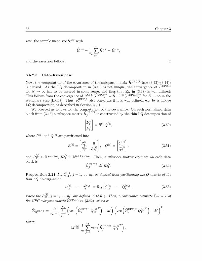
68 Chapter 3
with the sample mean vec Hcov with
Hcov =1
nb
nb∑
j=1
Hcovj = Hcov,
and the assertion follows.
3.5.2.3 Data-driven case
Now, the computation of the covariance of the subspace matrix HUPC,R (see (3.43)–(3.44))is derived. As the LQ decomposition in (3.43) is not unique, the convergence of HUPC,R
for N → ∞ has to be assured in some sense, and thus that ΣH in (3.38) is well-defined:This follows from the convergence of HUPC(HUPC)T = HUPC,R(HUPC,R)T for N →∞ in thestationary case [BM07]. Thus, HUPC,R also converges if it is well-defined, e.g. by a uniqueLQ decomposition as described in Section 3.2.1.
We proceed as follows for the computation of the covariance. On each normalized datablock from (3.46) a subspace matrix HUPC,R
j is constructed by the thin LQ decomposition of
[Y−jY+j
]= R(j)Q(j), (3.50)
where R(j) and Q(j) are partitioned into
R(j) =
[R
(j)11 0
R(j)21 R
(j)22
], Q(j) =
[Q
(j)1
Q(j)2
], (3.51)
and R(j)11 ∈ Rqr0×qr0 , R
(j)21 ∈ R(p+1)r×qr0 . Then, a subspace matrix estimate on each data
block isHUPC,Rj
def= R
(j)21 . (3.52)
Proposition 3.21 Let Q(j)11 , j = 1, . . . , nb, be defined from partitioning the Q matrix of the
thin LQ decomposition[R
(1)11 . . . R
(nb)11
]= R11
[Q
(1)11 . . . Q
(nb)11
], (3.53)
where the R(j)11 , j = 1, . . . , nb, are defined in (3.51). Then, a covariance estimate ΣHUPC,R of
the UPC subspace matrix HUPC,R in (3.42) writes as
ΣHUPC,R =N
nb − 1
nb∑
j=1
(vec
(HUPC,Rj Q
(j)11
T)−M
)(vec
(HUPC,Rj Q
(j)11
T)−M
)T,
where
Mdef=
1
nb
nb∑
j=1
vec
(HUPC,Rj Q
(j)11
T).
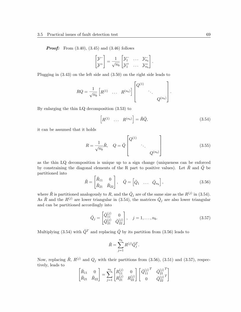
3.5 Practical issues of fault detection test 69
Proof: From (3.40), (3.45) and (3.46) follows
[Y−Y+
]=
1√nb
[Y−1 . . . Y−nbY+1 . . . Y+
nb
].
Plugging in (3.43) on the left side and (3.50) on the right side leads to
RQ =1√nb
[R(1) . . . R(nb)
]Q(1)
. . .
Q(nb)
.
By enlarging the thin LQ decomposition (3.53) to
[R(1) . . . R(nb)
]= RQ, (3.54)
it can be assumed that it holds
R =1√nbR, Q = Q
Q(1)
. . .
Q(nb)
(3.55)
as the thin LQ decomposition is unique up to a sign change (uniqueness can be enforcedby constraining the diagonal elements of the R part to positive values). Let R and Q bepartitioned into
R =
[R11 0
R21 R22
], Q =
[Q1 . . . Qnb
], (3.56)
where R is partitioned analogously to R, and the Qj are of the same size as the R(j) in (3.54).As R and the R(j) are lower triangular in (3.54), the matrices Qj are also lower triangularand can be partitioned accordingly into
Qj =
[Q
(j)11 0
Q(j)21 Q
(j)22
], j = 1, . . . , nb. (3.57)
Multiplying (3.54) with QT and replacing Q by its partition from (3.56) leads to
R =
nb∑
j=1
R(j)QTj .
Now, replacing R, R(j) and Qj with their partitions from (3.56), (3.51) and (3.57), respec-tively, leads to [
R11 0
R21 R22
]=
nb∑
j=1
[R
(j)11 0
R(j)21 R
(j)22
][Q
(j)11
TQ
(j)21
T
0 Q(j)22
T
]

70 Chapter 3
and hence
R21 =
nb∑
j=1
R(j)21 Q
(j)11
T.
Then, together with (3.44), (3.52), (3.55) and (3.56) it follows
HUPC,R =1√nb
nb∑
j=1
HUPC,Rj Q
(j)11
T. (3.58)
Now, regarding the vec(HUPC,Rj Q
(j)11
T), j = 1, . . . , nb, as i.i.d., the relation
ΣHUPC,R = N cov
(vec
(HUPC,R
1 Q(1)11
T))
follows analogously to (3.49) and the assertion follows.
This covariance computation of the data-driven subspace matrix is applied in Section 9.2for uncertainty quantification.
The difficulty for computing the covariance in the data-driven case lies in the non-uniqueness of the LQ decomposition and in the absence of a straightforward relation betweenHUPC,R and HUPC,R
j . In this context, also other approaches could be considered, as link-
ing the covariance computation of the vectorizations of HUPC,R and HUPC,R(HUPC,R)T =HUPC(HUPC)T or employing the matrix
Y+Y−T (Y−Y−T )−1/2,
which is related to HUPC,R by post-multiplying with an orthogonal matrix.
3.6 Conclusions
In this chapter, some basic numerical tools were introduced that are needed throughout thiswork. Additional properties of the statistical fault detection test from Section 2.3 were shownand clarified, deepening the theoretical understanding of this algorithm. Furthermore, somevery practical issues of the χ2-test computation were solved that are related to the handlingof a rank deficient estimate of the covariance matrix. This situation often appears when usingquite short data sets. A numerically robust implementation was suggested. The computationof the covariance matrix itself was detailed for covariance-driven SSI and extended to data-driven SSI with the UPC algorithm. These points increase the applicability of the faultdetection test in practice.
3.7 Dissemination
Parts of this chapter have been published in:

3.7 Dissemination 71
[DM11d] M. Dohler and L. Mevel. Robust subspace based fault detection. In Proc.18th IFAC World Congress, Milan, Italy, 2011.

72 Chapter 3

Part II
System identification
73


Chapter 4
Modular subspace-based systemidentification from multi-setup
measurements
4.1 Introduction
Subspace-based system identification methods have been proven efficient for the identificationof the eigenstructure of linear multivariable systems [BF85, Vib95, VODM96, PDR99, BM07].An important application of these methods is structural vibration analysis, where the vi-brating characteristics (modes, mode shapes) are identified of mechanical, civil or aero-nautical structures subject to uncontrolled, unmeasured and non-stationary excitation[HVdA99, MBG03].
To obtain vibration measurements at many coordinates of a structure with only fewsensors, it is common practice to use multiple sensor setups for the measurements. For thesemulti-setup measurements, some of the sensors, the so-called reference sensors, stay fixedthroughout all the setups, while the other sensors are moved from setup to setup. By fusingin some way the corresponding data, this allows to perform modal identification as if therewas a very large number of sensors, even in the range of a few hundreds or thousands.
Processing multi-setup measurement data for structural analysis is often achieved byperforming eigenstructure identification for each record separately, and then merging theresults obtained for records corresponding to different sensor pools. However, pole matchingmay be not easy in practice, and thus the result of eigenvector gluing may not be consistent[MK00, VdALMH00, CGDV02]. Therefore the question arises to perform eigenstructureidentification by merging the data of the successive records and processing them globally,instead of merging the identification results.
Global merging approaches in frequency domain were proposed for maximum likelihood

76 Chapter 4
identification in [PGC03] and for NExT-ERA in [Bro03, SF09]. In time domain, an empir-ical global merging approach for covariance-driven subspace identification was proposed in[RMDRC09].
In [MBBG02a, MBBG02b] a merging scheme was proposed for the covariance-drivenstochastic subspace identification and the non-stationary consistency of the resulting iden-tification algorithm was proved. We generalize the merging approach from [MBBG02a,MBBG02b], which is only designed for the covariance-driven stochastic subspace identifi-cation, to arbitrary subspace-based identification algorithms.1 Moreover, the new approachis modular, i.e. the data records from different setups are processed one after another insteadof together at the same time, in order to do global system identification. Furthermore, ascalable modular merging algorithm is proposed in this chapter, which uses only little morethan the memory needed for single-setup system identification of the setup actually beingprocessed. Like this, there are practically no limitations on the number of setups or sensorsthat can be processed. Non-stationary consistency of the proposed algorithms is proved forthe general class of subspace algorithms in [BM07].
In Operational Modal Analysis the true system order is unknown and recommendedtechniques from statistics to estimate the best model order (AIC, BIC, MDL, . . . ) may lead toa model with the best prediction capacity. However, one is rather interested in distinguishingbetween true physical modes and noise modes of the investigated system. For doing this,the identification procedure is repeated while truncating at different over-specified modelorders, as the noise modes tend to vary at different orders [PDR99]. In the classical subspacealgorithm, the model obtained by the selection of some lower order from an overestimatedhigher model order coincides with the direct truncation at this given order. We prove thesame property for the proposed merging algorithms.
This chapter is organized as follows. In Section 4.2, the general subspace-based systemidentification algorithm is introduced and two examples of stochastic subspace identificationalgorithms are given. In Section 4.3, the merging problem for multi-setup measurements isaddressed. The merging algorithm for the covariance-driven stochastic subspace identificationfrom [MBBG02a, MBBG02b] is generalized in two steps to arbitrary subspace-based systemidentification algorithms and the scalable merging algorithm is derived. In Section 4.4, non-stationary consistency of the proposed merging algorithms is proved, with the condition ofthe underlying subspace algorithm being consistent to non-stationary excitation [BM07]. InSection 4.5, the robustness of these algorithms to misspecified model order is investigated. InSection 4.6, implementation details are given for the merging algorithms using data-drivensubspace identification. Finally, in Section 4.7, the modal analysis of a bridge from vibra-tion measurements is considered as an application of the merging algorithms, before someconcluding remarks.
4.2 Subspace-based system identification
In this section, the basic principles of subspace-based system identification are recalled fromSection 2.2.2. We consider linear multivariable systems described by a discrete time state
1A slight mistake in the merging procedure in [MBBG02a, MBBG02b] is also corrected in this chapter.
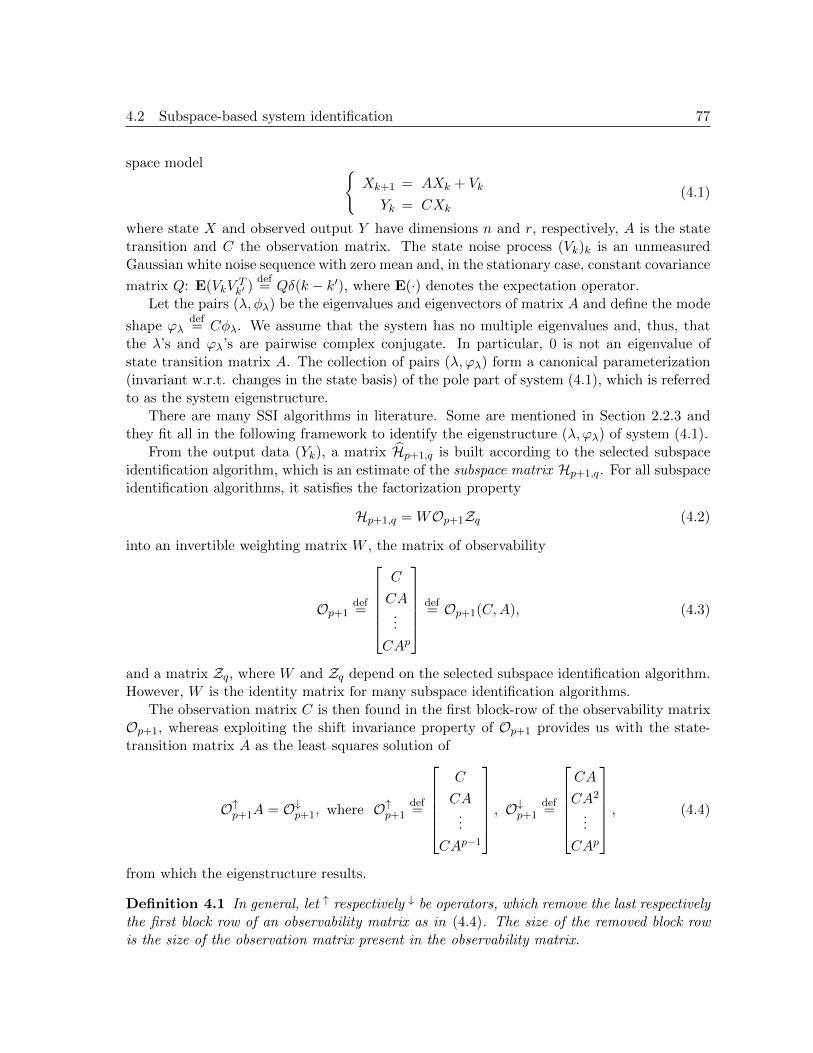
4.2 Subspace-based system identification 77
space model Xk+1 = AXk + Vk
Yk = CXk
(4.1)
where state X and observed output Y have dimensions n and r, respectively, A is the statetransition and C the observation matrix. The state noise process (Vk)k is an unmeasuredGaussian white noise sequence with zero mean and, in the stationary case, constant covariance
matrix Q: E(VkVTk′ )
def= Qδ(k − k′), where E(·) denotes the expectation operator.
Let the pairs (λ, φλ) be the eigenvalues and eigenvectors of matrix A and define the mode
shape ϕλdef= Cφλ. We assume that the system has no multiple eigenvalues and, thus, that
the λ’s and ϕλ’s are pairwise complex conjugate. In particular, 0 is not an eigenvalue ofstate transition matrix A. The collection of pairs (λ, ϕλ) form a canonical parameterization(invariant w.r.t. changes in the state basis) of the pole part of system (4.1), which is referredto as the system eigenstructure.
There are many SSI algorithms in literature. Some are mentioned in Section 2.2.3 andthey fit all in the following framework to identify the eigenstructure (λ, ϕλ) of system (4.1).
From the output data (Yk), a matrix Hp+1,q is built according to the selected subspaceidentification algorithm, which is an estimate of the subspace matrix Hp+1,q. For all subspaceidentification algorithms, it satisfies the factorization property
Hp+1,q = WOp+1Zq (4.2)
into an invertible weighting matrix W , the matrix of observability
Op+1def=
C
CA...
CAp
def= Op+1(C,A), (4.3)
and a matrix Zq, where W and Zq depend on the selected subspace identification algorithm.However, W is the identity matrix for many subspace identification algorithms.
The observation matrix C is then found in the first block-row of the observability matrixOp+1, whereas exploiting the shift invariance property of Op+1 provides us with the state-transition matrix A as the least squares solution of
O↑p+1A = O↓p+1, where O↑p+1def=
C
CA...
CAp−1
, O↓p+1
def=
CA
CA2
...
CAp
, (4.4)
from which the eigenstructure results.
Definition 4.1 In general, let ↑ respectively ↓ be operators, which remove the last respectivelythe first block row of an observability matrix as in (4.4). The size of the removed block rowis the size of the observation matrix present in the observability matrix.

78 Chapter 4
The actual implementation of this generic subspace identification algorithm uses a con-sistent estimate Hp+1,q obtained from the output data according to the selected subspaceidentification algorithm. The SVD
Hp+1,q =[U1 U0
] [∆1 0
0 ∆0
][V T1
V T0
](4.5)
and its truncation at the model order n yields an estimate Op+1 = W−1U1∆1/21 for the
observability matrix, from which (C, A) and (λ, ϕλ) are recovered as sketched above. Also,
the estimate Zq = ∆1/21 V T
1 can be obtained.
For simplicity, let p and q be given, and the subscripts of Hp+1,q, Op+1 and Zq may beskipped.
4.3 Multi-setup stochastic subspace identification
In this section, the state-space model for multi-setup measurements is introduced andthe problem of merging data from different setups is stated. The merging scheme from[MBBG02a, MBBG02b] for the covariance-driven subspace identification algorithm is pre-sented and generalized to subspace identification algorithms without a left weighting (W = I).In Algorithm 4.3 a modular version of this algorithm is derived, where the records of the dif-ferent setups are processed one after another, instead of altogether, for a practical implemen-tation and less numerical operations. In the next step, Algorithm 4.4 is derived that mergesthe observability matrices obtained from the different records to a global observability matrixand thus can be applied to arbitrary subspace identification algorithms. Finally, a scalablecomputation of the system matrices is derived for Algorithm 4.4 in the case of a large numberof sensors and setups.
4.3.1 Modeling multi-setup measurements
Instead of a single record for the output (Yk) of the system (4.1), Ns records
(Y
(1,ref)k
Y(1,mov)k
)
︸ ︷︷ ︸Record 1
(Y
(2,ref)k
Y(2,mov)k
)
︸ ︷︷ ︸Record 2
. . .
(Y
(Ns,ref)k
Y(Ns,mov)k
)
︸ ︷︷ ︸Record Ns
(4.6)
are now available collected successively. Each record j contains data Y(j,ref)k of dimension r(ref)
from a fixed reference sensor pool, and data Y(j,mov)k of dimension r(j) from a moving sensor
pool. Then, the total number of sensor positions is r(all)def= r(ref)+
∑Nsj=1 r
(j). For each setup j,this corresponds to observing the state space system (4.1) at different sets of time instants k,where the observation matrices are different for every setup. The transition matrix A remainsthe same, since the same system is observed. As the sensor settings for the moving sensorschange, the respective observation matrices mapping the states to the observations at the

4.3 Multi-setup stochastic subspace identification 79
moving sensors are different for each setup j, while the observation matrix with respect tothe reference sensors stays the same for all setups. Denote the former observation matricesby C(j,mov) ∈ Rr(j)×n, j = 1, . . . , Ns, and the latter by C(ref) ∈ Rr(ref)×n. Furthermore, denote
the states Xk and state noise Vk from system (2.1) corresponding to record j by X(j)k and
V(j)k , respectively. Thus, to each record j = 1, . . . , Ns corresponds a state-space realization
in the form [MBBG02a, MBBG02b]
X(j)k+1 = A X
(j)k + V
(j)k
Y(j,ref)k = C(ref) X
(j)k (reference pool)
Y(j,mov)k = C(j,mov) X
(j)k (sensor pool noj)
(4.7)
Define the global observation matrix containing information of all the sensor positions as
C(all) def=
C(ref)
C(1,mov)
C(2,mov)
...
C(Ns,mov)
∈ Rr
(all)×n, (4.8)
corresponding to C in (4.1).
Definition 4.2 A subspace matrix H(j) is called local subspace matrix of record j, if itsestimate is built from the output data
Y(j)k
def=
[Y
(j,ref)k
Y(j,mov)k
]
with a selected subspace identification algorithm, and whose associated observability matrixin (4.2) is the local observability matrix
O(j) def= O
([C(ref)
C(j,mov)
], A
), (4.9)
cf. the definition of O in (4.3). A subspace matrix H(all) is called global subspace matrix, if its
associated observability matrix in (4.2) is the global observability matrix O(all) def= O(C(all), A).
4.3.2 The merging problem
In order to identify the eigenstructure of system (4.7) on the basis of the measurements (4.6),the output-only subspace algorithm of Section 4.2 has to be adapted. It is the aim to mergethe data from the different records prior to the identification step of the algorithm, so thatthe identification steps (4.2)–(4.4) only have to be done once. This corresponds to mergingthe local subspace matrices H(j), j = 1, . . . , Ns, to a global subspace matrix H(all), or merging

80 Chapter 4
the local observability matrices O(j) to a global observability matrix O(all), which is the mainproblem in this chapter. Then, the eigenstructure of system (4.7) can be obtained from anidentified pair of system matrices (C(all), A) by applying the generic subspace algorithm ofSection 4.2 on H(all) or on O(all).
A cornerstone in Section 4.2 is factorization (4.2), which, of course, holds for each localsubspace matrix H(j) of the Ns records with a different observability matrix O(j) on the leftand in general a different matrix Z(j) on the right side. If the matrices Z(j) were identical2
for all j = 1, . . . , Ns, interleaving block rows of the matrices H(j) would lead to a globalsubspace matrix having a factorization property (4.2) with Z = Z(j) on the right side, whichcould be used for global system identification.
However, there are several reasons for possible differences between the matrices Z(j):
In general, the matrices Z(j) are dependent on different sensor sets, as the movingsensor set is different for each setup j. Hence, the matrices Z(j) are different.
For most subspace algorithms, e.g. the data-driven algorithms in [VODM96] as UPC,the matrices Z(j) have no expected value as their size depends on the number of samples
N and the initial state X(j)0 , or they are not uniquely defined due to LQ decompositions
as in (2.13), so that in fact only some Z(j)Sj with unknown matrix Sj can be estimated.
The matrices O(j) and Z(j) might be in a different modal basis for each setup j, so thatin fact O(j)Tj and T−1j Z(j) are identified with an invertible unknown change of basismatrix Tj . This is also the reason why matrix (4.8) cannot be obtained straightforwardfrom a separate system identification of the measurement setups j = 1, . . . , Ns.
If the excitation V(j)k is uncontrolled, its covarianceQ(j) with E(V
(j)k V
(j)k′ ) = Q(j)δ(k−k′)
is record dependent. Hence, Z(j) is also dependent on Q(j), which can be differentfor each record. This case appears especially in practice when ambient excitation isconsidered. Multi-setup measurements take place over a longer time period than asingle measurement and it is likely that properties of the ambient excitation changebetween the measurement campaigns.
By normalizing the data in a certain way, it can be achieved that the corresponding
matrices Z(j)are identical for all the records. Thus, the corresponding normalized subspace
matrices can be merged into a global subspace matrix, on which system identification of thewhole system can be done. This is the basic idea of the merging algorithms presented in thefollowing sections.
2By nature, the Z(j)’s are indeed identical for j = 1, . . . , Ns in covariance-driven subspace identificationunder stationary excitation throughout all setups using correlations R
(j)i = E(Y
(j)k Y
(j,ref)Tk−i ) in (2.8). However,
this is a very special case.

4.3 Multi-setup stochastic subspace identification 81
4.3.3 Merging for covariance-driven SSI from [MBBG02a, MBBG02b]
For each setup j, the two families of cross-correlations
R(j,ref)i
def= E
(Y
(j,ref)k Y
(j,ref)Tk−i
), (4.10)
R(j,mov)i
def= E
(Y
(j,mov)k Y
(j,ref)Tk−i
)(4.11)
are defined. From their definition, they enjoy the factorization properties
R(j,ref)i = C(ref)AiG(j), R
(j,mov)i = C(j,mov)AiG(j), (4.12)
where G(j) def= E
(X
(j)k Y
(j,ref)Tk−i
)is the cross-correlation between the state and the reference
outputs of setup j.
In the stationary case, the state-output cross-correlations G(j) are equal for all the setups,G = G(j), j = 1, . . . , Ns. Consequently, the cross-correlations of the outputs can be stackedto a block column vector
R(all)i =
R(1,ref)i
R(1,mov)i
...
R(Ns,mov)i
for each lag i, which factorizes as R(all)i = C(all)AiG. The corresponding block Hankel ma-
trix (see Equation (2.8)) filled with these correlations factorizes as H(all) def= Hank(R
(all)i ) =
O(C(all), A)C(A,G). Thus, the global system identification can be performed on this mergedmatrix. However, this merging approach fails in the non-stationary case, as stressed in[MBBG02a, MBBG02b].
In the non-stationary case, some normalization of the data has to be performed priorto merging. This happens in two steps: First, the factors Z(j) of the subspace matrixfactorization are identified in the same modal basis, and second, the data of all setups isnormalized and merged using the factors Z(j).
Thanks to factorization property (4.12), the block Hankel matrices built from the cross-correlations of the output data in (4.10) and (4.11) factorize as
H(j,ref) def= Hank(R
(j,ref)i ) = O(C(ref), A) C(A,G(j)),
H(j,mov) def= Hank(R
(j,mov)i ) = O(C(j,mov), A) C(A,G(j)). (4.13)
Note that a local subspace matrix H(j) as in Definition 4.2 can be obtained from interleavingthe block rows of H(j,ref) and H(j,mov), and factorization property H(j) = O(j)Z(j) holds withZ(j) = C(A,G(j)). These factors C(A,G(j)) are obtained as follows. Let
R(all,ref)i
def=[R
(1,ref)i . . . R
(Ns,ref)i
](4.14)

82 Chapter 4
be the block row vector of the reference data correlations of all setups. It factorizes as
R(all,ref)i = C(ref)AiG(all), G(all) def
=[G(1) . . . G(Ns)
].
The corresponding block Hankel matrix, which factorizes as
H(all,ref) def= Hank(R
(all,ref)i ) = O(C(ref), A) C(A,G(all)), (4.15)
can be obtained by interleaving block columns of H(j,ref), j = 1, . . . , Ns. Assume that thepair (C(ref), A) is observable. The factors
C(A,G(j)) =[G(j) AG(j) . . . Aq−1G(j)
]
are then obtained by juxtaposing the appropriate block columns of C(A,G(all)), which ispartitioned as
C(A,G(all)) =[G(1) . . . G(Ns) AG(1) . . . AG(Ns) . . . Aq−1G(1) . . . Aq−1G(Ns)
].
(4.16)For doing so, note that C(A,G(all)) has to be partitioned differently than stated in [MBBG02a,MBBG02b].
Assume that for all j the pair (A,G(j)) is controllable and that, up to a permutationon the record indices, C(A,G(1)) is the best conditioned controllability matrix among theC(A,G(j))’s. Then, the right factor C(A,G(j)) in (4.13) is removed and replaced by C(A,G(1))in the normalized matrices
H(j,mov) def= H(j,mov)C(A,G(j))T (C(A,G(j))C(A,G(j))T )−1C(A,G(1)),
as defined in [MBBG02a, MBBG02b]. This notation can be simplified by using the pseudoin-verse:
H(j,mov)= H(j,mov)C(A,G(j))†C(A,G(1)). (4.17)
The normalized matrix H(j,mov)then corresponds to a block Hankel matrix filled with nor-
malized cross-correlations R(j,mov)i = C(j,mov)AiG(1), which can be stacked for the different
setups, together with the cross-correlation of the reference sensors, to
R(all)i
def=
R(1,ref)i
R(1,mov)i
...
R(Ns,mov)i
= C(all)AiG(1), (4.18)
similar to the stationary case. Hence, the corresponding block Hankel matrix H(all)filled
with these correlations fulfills the desired factorization property
H(all) def= Hank(R
(all)i ) = O(C(all), A)C(A,G(1))
and therefore can be used for the global system identification from Section 4.2. This normal-
ized and merged matrix H(all)can be obtained by interleaving the block rows of H(1,ref) and
H(j,mov), j = 1, . . . , Ns.
The merging algorithm described in this section is summarized in Algorithm 4.1.

4.3 Multi-setup stochastic subspace identification 83
Algorithm 4.1 Multi-setup merging for covariance-driven SSI
Input: Subspace matrix estimates for setups j = 1, . . . , Ns :
H(j,ref) = Hank(R(j,ref)i ) Equation (4.10)
H(j,mov) = Hank(R(j,mov)i ) Equation (4.11)
1: Build H(all,ref) by interleaving the block columns of H(j,ref), j = 1, . . . , Ns, analogously to(4.14)
2: SVD of H(all,ref) = U ΣV T and keep C(all) def= C(A,G(all)) = Σ1/2V T Equation (4.15)
3: Partition C(all) =[C(1,1) . . . C(1,Ns) C(2,1) . . . C(2,Ns) . . . C(q,Ns)
], where each
block has r(ref) columns, and set Cj =[C(1,j) . . . C(q,j)
], j = 1, . . . , Ns Equ. (4.16)
4: Compute H(j,mov) = H(j,mov)C†j C1 Equation (4.17)5: Build H(all) by interleaving the block rows of H(1,ref) and H(j,mov), j = 1, . . . , Ns, analo-
gously to (4.18)
Output: Global subspace matrix H(all) for system identification
4.3.4 Generalization of merging algorithm to SSI algorithms with W = I
Now, the merging approach from the previous section is generalized to subspace identificationalgorithms satisfying (4.2) with W = I, i.e. without a left weighting. From the outputdata of the Ns measurement setups of system (4.7), the respective local subspace matricesH(j) = O(j)Z(j) as in Definition 4.2 are built based on the selected algorithm. Again, it isthe aim to obtain a global subspace matrix H(all) from them in order to do a global systemidentification.
First, for each setup j, the local subspace matrix H(j) is separated into the referencesensor part H(j,ref) and the moving sensor part H(j,mov) by selecting the appropriate blockrows, such that the factorization properties
H(j,ref) = O(C(ref), A)Z(j), (4.19)
H(j,mov) = O(C(j,mov), A)Z(j) (4.20)
hold. Assume that (C(ref), A) is observable. Juxtaposing the matrices H(j,ref), j = 1, . . . , Ns,to
H(all,ref) def=[H(1,ref) . . . H(Ns,ref)
](4.21)
– instead of interleaving their block columns as in Algorithm 4.1 –, yields a matrix withfactorization property
H(all,ref) = O(C(ref), A)[Z(1) . . . Z(Ns)
](4.22)
similar to (4.15), from which the matrices Z(1), . . . ,Z(Ns) can be recovered in the same modalbasis.
Assume that all the Z(j)’s are full row rank, and similarly to Algorithm 4.1, that Z(1)
is the best conditioned matrix among the Z(j)’s. Then, the right factor Z(j) in (4.20) is

84 Chapter 4
removed and replaced by Z(1) in the normalized matrices
H(j,mov) def= H(j,mov)Z(j)†Z(1), (4.23)
similar to (4.17), and factorization property H(j,mov)= O(C(j,mov), A)Z(1) follows. Hence,
interleaving the block rows of H(1,ref) and H(j,mov), j = 1, . . . , Ns, yields the desired global
subspace matrix
H(all) def= P
H(1,ref)
H(1,mov)
...
H(Ns,mov)
= O(C(all), A)Z(1), (4.24)
where P is a suitable permutation matrix.
The merging algorithm described in this section is summarized in Algorithm 4.2.
Algorithm 4.2 Multi-setup merging for SSI algorithms without left weighting
Input: Local subspace matrix estimates H(j) for setups j = 1, . . . , Ns Definition 4.21: Separate H(j) into H(j,ref) and H(j,mov), j = 1, . . . , Ns Equations (4.19), (4.20)2: Juxtapose H(j,ref), j = 1, . . . , Ns, to H(all,ref) =
[H(1,ref) . . . H(Ns,ref)
]Equ. (4.21)
3: SVD of H(all,ref) =[U1 U0
] [∆1 0
0 ∆0
][V T1
V T0
], keep Z(all) def
= ∆1/21 V T
1 and recover Z(j),
j = 1, . . . , Ns, from partitioning Z(all) =[Z(1) . . . Z(Ns)
]Equation (4.22)
4: Compute H(j,mov) = H(j,mov)Z(j)†Z(1) Equation (4.23)5: Build H(all) by interleaving the block rows of H(1,ref) and H(j,mov), j = 1, . . . , Ns
Equation (4.24)Output: Global subspace matrix H(all) for system identification
4.3.5 Modular merging algorithm for SSI algorithms with W = I
For obtaining the right factors Z(j) in (4.22), the subspace matrices of all the setups j =1, . . . , Ns need to be in memory at the same time. This can be a problem in the case of alarge number of setups or when it is impractical to access data from different setups at thesame time. With the help of the following lemma, this step can be avoided, thus leading toa more efficient merging procedure.
Lemma 4.3 For each setup j ∈ 1, . . . , Ns let H(j,ref) be given, which is obtained from thelocal subspace matrix H(j) and fulfills factorization property (4.19). Assume that the pair(C(ref), A) is observable, i.e. O(C(ref), A) is full column rank, and Z(j) is full row rank. Then,
Z(j)†Z(1) = H(j,ref)†H(1,ref).

4.3 Multi-setup stochastic subspace identification 85
Proof: From factorization property (4.19) follows
H(j,ref)† = Z(j)†O(C(ref), A)†,
as O(C(ref), A) is full column rank and Z(j) is full row rank. Post-multiplyingH(1,ref) = O(C(ref), A)Z(1) leads to the assertion, again because O(C(ref), A) is fullcolumn rank.
Lemma 4.3 makes the explicit computation of the factors Z(j) unnecessary for the nor-malization in (4.23), which is then equivalent to
H(j,mov)= H(j,mov)H(j,ref)†H(1,ref). (4.25)
The resulting modular merging algorithm is summarized in Algorithm 4.3, where the data ofthe different setups is processed setup after setup, instead of altogether while only keepingH(1,ref) in memory all the time.
Algorithm 4.3 Modular multi-setup merging for SSI algorithms without left weighting
Input: Local subspace matrix estimates H(j) for setups j = 1, . . . , Ns Definition 4.21: for j = 1 to Ns do2: Separate H(j) into H(j,ref) and H(j,mov) Equations (4.19), (4.20)3: Compute H(j,mov) = H(j,mov)H(j,ref)†H(1,ref) Equation (4.25)4: end for5: Build H(all) by interleaving the block rows of H(1,ref) and H(j,mov), j = 1, . . . , Ns
Equation (4.24)Output: Global subspace matrix H(all) for system identification
4.3.6 Generalized merging algorithm for arbitrary SSI algorithms
Let the local subspace matrices H(j), j = 1, . . . , Ns according to Definition 4.2 for anysubspace identification algorithm be given, which fulfill the factorization property
H(j) = W (j)O(j)Z(j) (4.26)
as in (4.2), with an invertible weighting matrix W (j), for any setup j. The respective localobservability matrices O(j), which can be obtained from H(j) as described in Section 4.2, are
now used for merging in order to obtain a global observability matrix O(all) def= O(C(all), A), on
which the system identification can be done. This is slightly different from the last sections,where it was the aim to obtain a global subspace matrix H(all).
As the local observability matrices are obtained from the local subspace matrices for eachsetup separately, they might be in different modal bases, so in fact onlyO(j)Tj can be obtainedfrom H(j), where Tj is an invertible change of basis matrix. The problem for merging regardsnow the different factors Tj instead of the different factors Z(j) as previously.

86 Chapter 4
For any j, the matrix O(j) fulfills property (4.9) and hence can be separated intoO(C(ref), A) and O(C(j,mov), A) by choosing the appropriate block rows of O(j). Hence, sep-arating O(j)Tj in the same way leads to
O(j,ref) def= O(C(ref), A)Tj , O(j,mov) def
= O(C(j,mov), A)Tj . (4.27)
Assume that in each setup j the pair (C(ref), A) is observable, i.e. O(j,ref) is full columnrank. A common modal basis for all setups can then be defined by the chosen modal basis ofone of the setups. Without loss of generality, let this be setup 1, for which T1 = I is defined asthe identity matrix, and hence O(1,ref) = O(C(ref), A). Another possibility to define a commonmodal basis is to make use of all the reference parts of the local observability matrices O(j,ref),to juxtapose them and obtain O(C(ref), A) through the factorization
[O(1,ref) . . . O(Ns,ref)
]= O(C(ref), A)
[T1 . . . TNs
]
by an SVD. In both ways, the obtained matrix O(C(ref), A) defines the modal basis, intowhich the other observability matrices have to be converted prior to merging.
Lemma 4.4 For each setup j ∈ 1, . . . , Ns let O(j,ref) and O(j,mov) be defined as in (4.27),and let (C(ref), A) be observable. Then,
O(C(j,mov), A) = O(j,mov)O(j,ref)†O(C(ref), A). (4.28)
Proof: From the first part of (4.27) follows O(j,ref)T−1j = O(C(ref), A) and hence
T−1j = O(j,ref)†O(C(ref), A),
as (C(ref), A) is observable and thus O(j,ref) is full column rank. Post-multiplying this to thesecond part of (4.27) leads to the assertion.
Lemma 4.4 provides a way to obtain the matrices O(C(j,mov), A), j = 1, . . . , Ns, which arein the same modal basis as O(C(ref), A). Hence, they can be merged together to the globalobservability matrix O(all) by interleaving their block rows
O(all) = P1
O(C(ref), A)
O(C(1,mov), A)...
O(C(Ns,mov), A)
= O(C(all), A), (4.29)
where P1 is a suitable permutation matrix as in (4.24). The resulting merging algorithm,which is suitable for arbitrary subspace identification algorithms, is summarized in Algorithm4.4, where the modal basis is defined by O(C(ref), A) = O(1,ref) in setup 1.

4.3 Multi-setup stochastic subspace identification 87
Algorithm 4.4 Multi-setup merging for arbitrary SSI algorithms
Input: Local subspace matrix estimates H(j) and weightings W (j) for setups j = 1, . . . , Ns
Equation (4.26)1: for j = 1 to Ns do
2: SVD and truncation at model order H(j) =[U1 U0
] [∆1 0
0 ∆0
][V T1
V T0
]Equ. (4.5)
3: Compute O(j) = W (j)−1U1∆1/21
4: Separate O(j) into O(j,ref) and O(j,mov) Equation (4.27)5: Compute O(j,mov) = O(j,mov)O(j,ref)†O(1,ref) Equation (4.28)6: end for7: Build O(all) by interleaving the block rows of O(1,ref) and O(j,mov), j = 1, . . . , Ns
Equation (4.29)Output: Observability matrix O(C(all), A) = O(all) for global system identification
4.3.7 Scalable computation of (C(all), A) for arbitrary SSI algorithms
In the previous section, the local subspace matrices H(j), j = 1, . . . , Ns, are used for thecomputation of a global observability matrix O(all), from which the system matrices (C(all), A)are recovered for system identification as described in Section 4.2: C(all) as the first blockrow of O(all), and A as the least squares solution of (4.4). However, if the number of sensorsand setups is large, the matrix O(all) may also be large, causing possibly memory problemswhen solving the least squares problem for A. In the following, an algorithm is described thatdirectly computes the system matrices (C(all), A) from the local subspace matrices, withoutcomputing O(all) explicitly.
Proposition 4.5 Let the thin QR decompositions and products
O(C(ref), A)↑ = Q0R0, S0def= QT0O(C(ref), A)↓, (4.30)
[Rj−1
O(C(j,mov), A)↑
]= QjRj , Sj
def= QTj
[Sj−1
O(C(j,mov), A)↓
], j = 1, . . . , Ns (4.31)
be given iteratively, where O(C(j,mov), A) is obtained from (4.28) during the iteration. Then,the least squares solution of O(all)↑A = O(all)↓ is given by
A = R−1NsSNs ,
and the parts of C(all) are recovered as the first block row of O(C(ref), A) and eachO(C(j,mov), A), j = 1, . . . , Ns, during the iteration.

88 Chapter 4
Proof: From (4.29) follows
O(all)↑ = P2
O(C(ref), A)↑
O(C(1,mov), A)↑
...
O(C(Ns,mov), A)↑
, O(all)↓ = P2
O(C(ref), A)↓
O(C(1,mov), A)↓
...
O(C(Ns,mov), A)↓
,
with the same permutation matrix P2 for both matrices. Thus, the least squares problem forA is equivalent to
O(C(ref), A)↑
O(C(1,mov), A)↑
...
O(C(Ns,mov), A)↑
A =
O(C(ref), A)↓
O(C(1,mov), A)↓
...
O(C(Ns,mov), A)↓
and the assertion follows from Lemma 3.8.
Note that after obtaining the local observability matrices of size (p+ 1)(r(ref) + r(j))× n,in this algorithm at no time matrices larger than (p ·maxr(j)+ n)× n are processed.
Then, from Proposition 4.5 the iterative computation of the system matrices is derivedin Algorithm 4.5.
Remark 4.6 In Proposition 4.5 and Algorithm 4.5 the estimate of the system matrix A isobtained iteratively at one specific model order from a least squares solution A = R−1S. Ifthe model order is unknown (cf. Section 4.5), the techniques from Chapter 5 can be used toobtain estimates of the system matrix at inferior model orders only by knowing the matricesR and S (cf. Section 5.3.5).
4.3.8 Some remarks
First, a remark is in order about the condition that the pair (C(ref), A) needs to be observablein all setups j = 1, . . . , Ns. This is a reasonable assumption, as it means that all the modes ofthe system need to be excited in the different data records, while the excitation may change.For the choice of the parameters in the identification algorithms it means that p has to bechosen such that Op+1(C
(ref), A)↑ = Op(C(ref), A) is full column rank in all setups, while thenumber of columns of Op(C(ref), A) is the model order n. A necessary condition is hencepr(ref) ≥ n. As parameter q for the subspace matrix (see e.g. (2.7) and (2.8)) is often set as
qdef= p + 1 [BBG+01], it may be useful to construct the local subspace matrices using the
fixed reference sensors as projection channels as in [PDR99] for an efficient implementation.An example is the covariance-driven merging algorithm in Section 4.3.3, where for each setupcross-correlations between all the sensor data and the reference sensor data are used. Anotherexample will be given in Section 4.6.2, where in the data matrices Y(j)− only data from thereference sensors is used.
Second, a remark should be made about the choice between the presented merging al-gorithms. Algorithm 4.1 is only suitable for the covariance-driven subspace identification.

4.3 Multi-setup stochastic subspace identification 89
Algorithm 4.5 Multi-setup merging for arbitrary SSI algorithms with iterative computationof system matrices
Input: Local subspace matrix estimates H(j) and weightings W (j) for setups j = 1, . . . , Ns
Equation (4.26)1: for j = 1 to Ns do
2: SVD and truncation at model order H(j) =[U1 U0
] [∆1 0
0 ∆0
][V T1
V T0
]Equ. (4.5)
3: Compute O(j) = W (j)−1U1∆1/21
4: Separate O(j) into O(j,ref) and O(j,mov) Equation (4.27)5: if j == 1 then6: QR decomposition of O(1,ref)↑ = QR7: Compute S = QT O(1,ref)↓
8: Extract C(ref) from first block row of O(1,ref) and keep it9: end if
10: Compute O(j,mov) = O(j,mov)O(j,ref)†O(1,ref) Equation (4.28)
11: QR decomposition of
[R
O(j,mov)↑
]= QR
12: Compute S = QT
[S
O(j,mov)↓
]
13: Set S = S, R = R
14: Extract C(j,mov) from first block row of O(j,mov) and keep it15: end for16: Compute A = R−1S17: Stack C(ref) and C(j,mov), j = 1, . . . , Ns, to C(all)
Output: A, C(all) system matrices after merging
Algorithms 4.2 and 4.3, which apply to any subspace identification algorithm without a leftweighting, differ in the order of data processing from the measurement setups and the num-ber of numerical operations. As Algorithm 4.3 does not need the SVD of the juxtaposedsubspace matrices related to the reference sensors and has a simpler structure, it is preferableto Algorithm 4.2. Algorithm 4.4 applies to arbitrary subspace identification algorithms. Be-sides the more general setting of Algorithm 4.4, it directly computes the global observabilitymatrix that is needed for the subspace identification. The scalable computation of the systemmatrices A and C in Algorithm 4.5 is an extension of Algorithm 4.4 and should be chosen inthe case of a very large number of sensors and setups when memory problems arise.
Third, a remark about the applicability of the presented algorithms is in order. Theonly condition of the merging algorithm to work with a subspace identification algorithm isfactorization property (4.2) of the respective subspace matrix, and the retrieval of the systemmatrices from the obtained observability matrix. This is a very general condition and applies,up to our knowledge, to all output-only subspace identification algorithms in literature. It

90 Chapter 4
also applies to combined deterministic-stochastic subspace identification algorithms, wheresome of the inputs of the system are known [VODM96], which is even a more general settingthan the output-only system identification considered in this chapter.
4.4 Non-stationary consistency
Until now, we have assumed stationary excitation within each record, but with a record-dependent covariance matrix. A more realistic assumption is that the excitation is non-
stationary within each record, i.e. the excitation covariance E(V(j)k V
(j)Tk′ )
def= Q
(j)k δ(k − k′)
is time-varying. We show that the merging algorithms can still be applied in this case ofnon-stationary excitation with only little modification. Then, the identified system matricesare consistent, once the subspace identification algorithm that is used to obtain the localsubspace matrices for each setup provides consistent estimates for the observation and statetransition matrices. The latter is the case, when the subspace identification algorithm fulfillsthe following assumption.
Assumption 4.7 For each record j there exists a triplet (C(j), A, Tj) and a sequence ofmatrices Tj(N), with Tj(N) and Tj(N)−1 uniformly bounded w.r.t. N , satisfying
C(j)(N)Tj(N) −→ C(j)Tj
Tj(N)−1Aj(N)Tj(N) −→ T−1j ATj
for N →∞, where
C(j) def=
[C(ref)
C(j,mov)
].
Matrix Tj denotes the modal basis defined by record j for N → ∞ where T1 = I, similar to
Tj(N) in (4.27). The pair (C(j)(N), Aj(N)) corresponds to (C, A), which is computed with
subspace system identification as in Section 4.2 from the local subspace matrix H(j) using Ndata samples.
Assumption 4.7 is satisfied under [BM07, Assumption 1] regarding the (stochastic) inputsand [BM07, Condition 2] regarding the chosen subspace algorithm. Notice that all subspacealgorithms mentioned in [BM07] satisfy these conditions, in particular the covariance-drivenand data-driven algorithm that are applied in this chapter, when the factor N in (2.10) and(4.41)–(4.42) is replaced by some value sN satisfying [BM07, Condition 2].
Theorem 4.8 Let the pair (C(all)(N), A(N)) correspond to (C(all), A) that can be recovered
from H(all) defined in Algorithm 4.3 or O(all) defined in Algorithm 4.4. Then, under As-sumption 4.7, there exists a pair (C(all), A) and a sequence of matrices T (N), with T (N) andT (N)−1 uniformly bounded w.r.t. N , satisfying
C(all)(N)T (N) −→ C(all),
T (N)−1A(N)T (N) −→ A
for N →∞.

4.5 Multi-setup identification under misspecified model order 91
Proof: From Assumption 4.7 follows
C(j,ref)(N)Tj(N) −→ C(ref)Tj
C(j,mov)(N)Tj(N) −→ C(j,mov)Tj
when separating C(j)(N) in its reference and moving sensor part, for any setup j. For therespective local observability matrices the convergence properties
O(C(ref)(N), Aj(N))Tj(N) −→ O(C(ref), A)Tj ,
O(C(j,mov)(N), Aj(N))Tj(N) −→ O(C(j,mov), A)Tj
follow and hence for the part of the global observability matrix in Step 5 of Algorithm 4.4
O(C(j,mov)(N), Aj(N))def= O(C(j,mov)(N), Aj(N))Tj(N)
(O(C(j,ref)(N), Aj(N))Tj(N)
)†
· O(C(1,ref)(N), A1(N))T1(N)
−→ O(C(j,mov), A)Tj
(O(C(ref), A)Tj
)†O(C(ref), A)T1
= O(C(j,mov), A).
Interleaving the block rows of O(C(1,ref)(N), A1(N))T1(N) and O(C(j,mov)(N), Aj(N)), j =1, . . . , Ns, and using (4.29), the assertion follows for Algorithm 4.4.
It remains the proof for Algorithm 4.3, when the pair (C(all)(N), A(N)) is recovered from
H(all). Then, under Assumption 4.7 it follows
H(j,ref) = O(C(ref)(N), Aj(N))Z(j)(N) + o(1),
where Z(j)(N) is the empirical counterpart of Z(j) in (4.19) and (4.20), and o(1) tends tozero when N →∞. With the same reasoning as above it follows
H(j,mov) = O(C(j,mov)(N), Aj(N))Z(1)(N) + o(1)
in Step 3 of Algorithm 4.3. Then, together with (4.24) and [BM07, Theorem 1] the assertionfollows for Algorithm 4.3.
The previous theorem proves non-stationary consistency for system identification withAlgorithms 4.3 and 4.4, once the underlying subspace method also provides non-stationaryconsistent estimates. The same holds for Algorithm 4.2, which provides equivalent results asAlgorithm 4.3, and Algorithm 4.5 which provides equivalent results as Algorithm 4.4.
4.5 Multi-setup identification under misspecified model order
In practice, the true system order is often unknown when data are recorded under operationalconditions. Recommended techniques from statistics to estimate the best model order arenot useful in this context. In order to retrieve a desired number of modes, a larger model

92 Chapter 4
order must be assumed. Then, the rank of the respective subspace matrices is hardly thetrue model order n, but full rank due to noise and a limited number of data samples. Thissection addresses two issues: First, the truncation at a desired model order in the mergingalgorithms, and second, the coherence of the merging algorithms during multi-order systemidentification, where the identification procedure is repeated while truncating at differentmodel orders n = nmin, . . . , nmax. The results of the multi-order identification are displayedin stabilization diagrams (see Section 2.4), where system modes can be distinguished fromnoise modes as the latter tend to vary at different orders.
4.5.1 Considering truncation due to noise
When deriving the merging algorithms, the order of the system was assumed to be a fixedvalue n, with all involved subspace matrices being of rank n. However, when subspacematrices are obtained from real data, the rank of the system usually cannot be determinedfrom them, as there is no drop in the singular values to zero due to noise and model reduction.Some assumption about the model order needs to be made for the identification, namely bythe selection of an order n in (4.23), on which Algorithm 4.3 is based, or O(j) in Algorithm 4.4.However, Algorithm 4.3 is based on Lemma 4.3, which assumes that factorization property(4.19) is fulfilled exactly. This is not the case when some system order n is assumed, which islower than the dimension of H(j,ref). In this case, Algorithm 4.3 needs to be slightly modified.
Lemma 4.9 For each setup j ∈ 1, . . . , Ns let H(j,ref) be given, which can be obtained fromthe local subspace matrix H(j). It holds
H(j,ref) = O(C(ref), A)Z(j) + U(j)0 ∆
(j)0 V
(j)T0
similar to factorization property (4.19), where a partitioned SVD of H(j,ref) at model order nis given by
H(j,ref) =[U
(j)1 U
(j)0
] [∆(j)1 0
0 ∆(j)0
][V
(j)T1
V(j)T0
].
Assume that the pair (C(ref), A) is observable, i.e. O(C(ref), A) is full column rank, and Z(j)
is full row rank. Then, it holds
Z(j)†Z(1) = H(j,ref)†,nH(1,ref),
where H(j,ref)†,n def= V
(j)1 ∆
(j)−11 U
(j)T1 denotes the truncated pseudoinverse of H(j,ref) at order n.
Proof: From the definition of the truncated pseudoinverse follows that H(j,ref)†,n isequal to Z(j)†O(C(ref), A)† and hence
H(j,ref)†,nH(1,ref) = Z(j)†Z(1) + Z(j)†O(C(ref), A)†U(1)0 ∆
(1)0 V
(1)T0 . (4.32)
As O(C(ref), A)Z(1) = U(1)1 ∆
(1)1 V
(1)T1 , it follows O(C(ref), A)† = Z(1)V
(1)1 ∆
(1)−11 U
(1)T1 .
Plugging this in (4.32), it is apparent that the second term is zero because of U(1)T1 U
(1)0 = 0,
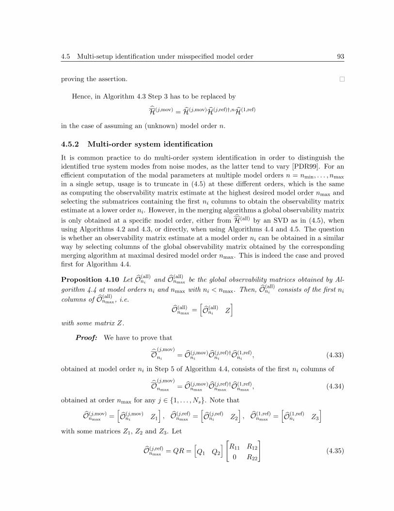
4.5 Multi-setup identification under misspecified model order 93
proving the assertion.
Hence, in Algorithm 4.3 Step 3 has to be replaced by
H(j,mov) = H(j,mov)H(j,ref)†,nH(1,ref)
in the case of assuming an (unknown) model order n.
4.5.2 Multi-order system identification
It is common practice to do multi-order system identification in order to distinguish theidentified true system modes from noise modes, as the latter tend to vary [PDR99]. For anefficient computation of the modal parameters at multiple model orders n = nmin, . . . , nmax
in a single setup, usage is to truncate in (4.5) at these different orders, which is the sameas computing the observability matrix estimate at the highest desired model order nmax andselecting the submatrices containing the first ni columns to obtain the observability matrixestimate at a lower order ni. However, in the merging algorithms a global observability matrix
is only obtained at a specific model order, either from H(all) by an SVD as in (4.5), whenusing Algorithms 4.2 and 4.3, or directly, when using Algorithms 4.4 and 4.5. The questionis whether an observability matrix estimate at a model order ni can be obtained in a similarway by selecting columns of the global observability matrix obtained by the correspondingmerging algorithm at maximal desired model order nmax. This is indeed the case and provedfirst for Algorithm 4.4.
Proposition 4.10 Let O(all)ni and O(all)
nmax be the global observability matrices obtained by Al-
gorithm 4.4 at model orders ni and nmax with ni < nmax. Then, O(all)ni consists of the first ni
columns of O(all)nmax, i.e.
O(all)nmax
=[O(all)ni Z
]
with some matrix Z.
Proof: We have to prove that
O(j,mov)
ni = O(j,mov)ni O(j,ref)†
ni O(1,ref)ni , (4.33)
obtained at model order ni in Step 5 of Algorithm 4.4, consists of the first ni columns of
O(j,mov)
nmax= O(j,mov)
nmaxO(j,ref)†nmax
O(1,ref)nmax
, (4.34)
obtained at order nmax for any j ∈ 1, . . . , Ns. Note that
O(j,mov)nmax
=[O(j,mov)ni Z1
], O(j,ref)
nmax=[O(j,ref)ni Z2
], O(1,ref)
nmax=[O(1,ref)ni Z3
]
with some matrices Z1, Z2 and Z3. Let
O(j,ref)nmax
= QR =[Q1 Q2
] [R11 R12
0 R22
](4.35)

94 Chapter 4
be the QR decomposition of O(j,ref)nmax , where Q and R are partitioned such that Q1 has ni
columns and R11 is of size ni × ni. Then, from (4.34) follows
O(j,mov)
nmax=[O(j,mov)ni Z1
] [R−111 −R−111 R12R−122
0 R−122
][QT1QT2
] [O(1,ref)ni Z3
]
=[O(j,mov)ni R−111 Z1
] [QT1 O(1,ref)ni QT1 Z3
QT2 O(1,ref)ni QT2 Z3
],
where Z1 = −O(j,mov)ni R−111 R12R
−122 + Z1R
−122 . From (4.35) follows
O(j,ref)ni = Q1R11 (4.36)
and hence QT2 O(j,ref)ni = 0. Then, from (4.27) follows QT2 O
(1,ref)ni = 0 and hence
O(j,mov)
nmax=[O(j,mov)ni R−111 Q
T1 O
(1,ref)ni Z2
],
where Z2 = O(j,mov)ni R−111 Q
T1 Z3 + Z1Q
T2 Z3. From (4.36) follows O(j,ref)†
ni = R−111 QT1 , leading
with (4.33) to the assertion.
Proposition 4.10 justifies the computation of the global observability matrix with Algo-rithm 4.4 at a maximal desired model order and the estimation at lower model orders directlyfrom this matrix, as it is done in subspace identification of a single setup. In a similar way,it can be shown that Algorithm 4.3 satisfies the same property:
Corollary 4.11 Let O(all)nmax and O(all)
ni be recovered from H(all)
nmaxand H
(all)
ni , which are obtainedfrom Algorithm 4.3 assuming model order nmax and ni, respectively, where in Algorithm 4.3
Lemma 4.9 is applied. Then, O(all)ni consists of the first ni columns of O(all)
nmax up to a changeof basis, i.e.
O(all)nmax
=[O(all)ni T Z
]
with some invertible matrix T and some matrix Z.
Proof: For each j = 1, . . . , Ns, in Algorithm 4.3 it follows together with Lemma 4.9
H(j,mov)
nmax= H(j,mov)H(j,ref)†,nmaxH(1,ref), H
(j,mov)
ni = H(j,mov)H(j,ref)†,niH(1,ref).
Similarly to Lemma 4.9 it can be shown that
H(j,mov)
nmax= O(j,mov)
nmaxO(j,ref)†nmax
O(1,ref)nmax
Z(1)nmax
,
H(j,mov)
ni = O(j,mov)ni O(j,ref)†
ni O(1,ref)ni Z(1)
ni
and hence
H(all)
nmax= O(all)
nmaxZ(1)nmax
, H(all)
ni = O(all)ni Z(1)
ni ,

4.6 Application of merging algorithms to data-driven SSI 95
using the notations of Proposition 4.10. From Proposition 4.10 follows O(all)nmax =
[O(all)ni Z
]
and as O(all)nmax and O(all)
ni are recovered directly from H(all)
nmaxand H
(all)
ni by an SVD, theassertion follows.
Proposition 4.10 and Corollary 4.11 justify the computation of the global subspace orobservability matrix using the Algorithms 4.3 or 4.4 only once at a maximal desired modelorder. Then, system identification is done at multiple lower model orders using this matrix.This is especially useful in vibration analysis of civil, mechanical or aeronautical structures,where multi-order identification helps to distinguish true structural modes from noise orspurious mathematical modes.
4.6 Application of merging algorithms to data-driven SSI
4.6.1 Size reduction with LQ decompositions
For so-called data-driven subspace identification algorithms such as the UPC algorithm inSection 2.2.3, the number of columns of the subspace matrix H is in the order of the availablesamples N , which is usually very big compared to the model order n. In this case, a thin LQdecomposition of the data like in (2.13) is done at first, leading to a factorization of subspacematrixH = HQ into the matrix H, whose number of columns is only in the order of the modelorder n, and a matrix Q containing orthonormal rows with QQT = I [VODM96, PDR99].Because of this property, the subspace identification algorithm from Section 4.2 can be calledusing H instead H, as the left side of the SVD (4.5), from which the observability matrixis retrieved, is not influenced by a different orthogonal matrix on the right side [VODM96].Hence, matrix H is also a subspace matrix fulfilling a factorization property (4.2). In practice,H instead of H is used for system identification, as it is in general much smaller (less columns)and its computation numerically more stable than the computation of H itself.
Now it is shown that the same size reduction of the local subspace matrices prior to usingmerging algorithms 4.2–4.5 is consistent, i.e. either using H(j), j = 1, . . . , Ns, or the matricesH(j), j = 1, . . . , Ns, with
H(j) = H(j)Qj , QjQTj = I, (4.37)
as local subspace matrices in the merging algorithms yields the same global system identifi-
cation results. Denote the respective global subspace matrices H(all) and H(all), respectively.
4.6.1.1 Algorithms 4.2 and 4.3
With Lemma 4.3, the normalization step in Algorithm 4.3 is equivalent to
H(j,mov) = H(j,mov)H(j,ref)†H(1,ref), (4.38)
using H(j), j = 1, . . . , Ns, and
H(j,mov) = H(j,mov)H(j,ref)†H(1,ref), (4.39)

96 Chapter 4
using H(j), j = 1, . . . , Ns. Separating the subspace matrices into reference and moving sensorparts leads with (4.37) to the relation
H(j,ref) = H(j,ref)Qj , H(j,mov) = H(j,mov)Qj .
Plugging this into (4.38) and using (4.39) leads to
H(j,mov) = (H(j,mov)Qj)(H(j,ref)Qj)†H(1,ref)Q1
= H(j,mov)H(j,ref)†H(1,ref)Q1 = H(j,mov)Q1
for j = 1, . . . , Ns. Furthermore, H(1,ref) = H(1,ref)Q1. Hence, because of (4.24), the merged
subspace matrices H(all) and H(all) enjoy the relation
H(all) = H(all)Q1, (4.40)
proving thatH(all) and H(all) yield the same global system identification results, as Q1QT1 = I.
4.6.1.2 Algorithms 4.4 and 4.5
Algorithms 4.4 and 4.5 compute the local observability matrix O(j), which is used for furthercomputations instead H(j) or H(j). Because of (4.37), the matrices U1 and ∆1, on which O(j)
is computed, can be assumed to be equal without loss of generality, either coming from H(j)
or H(j).3 Hence, global system identification results are the same for both H(j) and H(j).
4.6.2 Example: Multi-setup reference-based SSI with UPC algorithm
The data-driven Unweighted Principal Component (UPC) algorithm [VODM96], [PDR99] isa popular algorithm for stochastic system identification and was described in Section 2.2.3 fora single measurement setup. In this section, implementation details are given for multi-setupsystem identification with the reference-based UPC algorithm.
Choose p such that pr(ref) ≥ n and set q = p+ 1. For each setup j, the data matrices
Y(j)+ def=
1√N
Y(j)q+1 Y
(j)q+2 . . . Y
(j)N+q
Y(j)q+2 Y
(j)q+3 . . . Y
(j)N+q+1
......
. . ....
Y(j)q+p+1 Y
(j)q+p+2 . . . Y
(j)N+q+p
, (4.41)
Y(j)− def=
1√N
Y(j,ref)q Y
(j,ref)q+1 . . . Y
(j,ref)N+q−1
Y(j,ref)q−1 Y
(j,ref)q . . . Y
(j,ref)N+q−2
......
. . ....
Y(j,ref)1 Y
(j,ref)2 . . . Y
(j,ref)N
(4.42)
3By defining a unique SVD, where e.g. the first entries of the left singular vectors are positive values, thematrices U1 and ∆1 are identical in both SVDs of H(j) and H(j).

4.7 Structural vibration analysis example 97
are built, where
Y(j)k
def=
[Y
(j,ref)k
Y(j,mov)k
].
Note that in this reference-based version, matrix Y(j)− only contains data from the referencesensors of the setup, instead of data from all sensors. The local subspace matrix estimate isthen defined as
H(j) = Y(j)+Y(j)−T (Y(j)−Y(j)−T )†Y(j)−,
but not explicitly computed. Instead, the thin LQ decomposition[Y(j)−
Y(j)+
]=
[R
(j)11 0
R(j)21 R
(j)22
][Q
(j)1
Q(j)2
](4.43)
is performed, from which H(j) = R(j)21Q
(j)1 follows. Hence, (4.37) is satisfied with H(j) def
= R(j)21
and Qjdef= Q
(j)1 . Note that the number of columns of H(j) is only qr(ref), which is in general
significantly smaller than N .Then, the merging algorithms can be called using the matrices H(j), j = 1, . . . , Ns. In
the case of a moderate number of sensors and setups, Algorithm 4.3 should be used to obtainthe global subspace matrix, or Algorithm 4.4 should be used to obtain a global observabilitymatrix, from which the system matrices A and C(all) are retrieved. The scalable computationof the system matrices in Algorithm 4.5 should be used in the case of a large number ofsensors and setups.
It is stressed that using matrices H(j) in the merging algorithms is in general much moreefficient than using the matrices H(j), j = 1, . . . , Ns. It should be also noted that with relation
(4.40), the Kalman filter state matrix can be recovered from the merged matrix H(all) andthe orthogonal matrix Q1 from the first setup.
4.7 Structural vibration analysis example
An important instance of eigenstructure identification with subspace-based system identi-fication algorithms is the structural vibration analysis of mechanical structures [POB+91].In Operational Modal Analysis, the excitation of the structure cannot be measured and isuncontrolled, typically turbulent in nature and non-stationary. Typical examples are build-ings subject to wind, or bridges, dams and offshore structures subject to wind or swell. Themulti-setup system identification is of practical interest for these structures, as they can beobserved at many degrees of freedom, while only using a few sensors.
In Section 2.4, the underlying mechanical model and its respective discrete time state-space model were recalled. In the following, the structural vibration analysis example of[MBBG02b] is revisited using covariance-driven and data-driven stochastic subspace identi-fication, now showing very good eigenstructure identification results.
The proposed merging algorithms have been applied on vibrational data of the Z24 Bridge[MDR03], a benchmark of the COST F3 European network. The analyzed data is the responseof the bridge to ambient excitation (traffic under the bridge) measured in 154 points, mainly

98 Chapter 4
in the vertical and at some points also the transverse and lateral directions, and sampled at100 Hz. Because at most 33 sensors were available (counting one sensor for each measureddirection), Ns = 9 data sets have been recorded, each containing the measurements fromr(ref) = 5 fixed and 28 moving sensors, except dataset j = 5 containing only 22 moving sensors.Like this, altogether 251 sensors were mimicked. Each signal contains 65,535 samples.
The merging Algorithms 4.2–4.5 were derived for a wide range of subspace identificationalgorithms. Here, they are tested with subspace matrices from two popular identificationalgorithms, namely the covariance-driven (cf. Equation (4.13)) and the data-driven subspaceidentification with UPC (cf. Section 4.6.2). All available data from the nine setups was used,which includes sensor data from different directions at the same time. For the constructionof the subspace matrices, the parameters p+ 1 = q = 50 have been selected, thus leading tothe maximal possible model order pr(ref) = 245 of the system. The global subspace matricesobtained from Algorithm 4.3 and the global observability matrix obtained from Algorithm 4.4are then of size 12,550 × 250 and do not pose a memory problem yet for further processing.Note that in the scalable computation of the system matrices with Algorithm 4.5, at no timematrices larger than 1,650 × 250 are processed.
In order to separate the true system modes from the noise modes, system identificationwas done selecting model orders from 10 to the maximal possible order 245 at every 5 orders.Then, modes showing up at successive orders and fulfilling certain stabilization criteria, suchas low variability of natural frequency, damping values and mode shapes between successiveorders, low damping values etc., are considered as true system modes. Their frequencies areplotted in a stabilization diagram [PDR99] to support the selection of the estimated model.Thanks to the results of Section 4.5, this multi-order system identification is done by justselecting columns of the global observability matrix obtained from the merging algorithms atthe maximal desired system order, instead of redoing the merging at all desired orders. Thecorresponding stabilization diagram of the natural frequencies is presented in Figure 4.1.
Frequency
302520151050
200
150
100
50
Model order
Stabilization diagram
Figure 4.1 – Stabilization diagram: natural frequencies vs. model order from system identification with data-drivenUPC algorithm.

4.8 Conclusions 99
Table 4.1 – Frequencies (f) and damping coefficients (ρ) of obtained modes with covariance- and data-drivenapproach.
covariance-driven data-driven
Mode f (Hz) ρ (%) f (Hz) ρ (%)
1 3.856 0.73 3.860 0.84
2 4.884 1.36 4.893 1.28
3 9.784 1.28 9.774 1.32
4 10.31 1.65 10.33 1.89
5 12.29 3.40 12.33 3.08
6 13.02 3.93 13.08 3.32
7 17.25 5.36 17.37 7.29
8 19.23 2.75 19.21 2.99
9 19.74 4.49 19.62 3.99
10 26.69 4.94 26.75 4.21
The system identification results after applying the merging with Algorithms 4.3 and 4.4are practically equal for each subspace method, while the results differ slightly comparingdifferent subspace methods. The obtained frequencies and damping coefficients from thecovariance- and the data-driven algorithm are summarized in Table 4.1. The differences inthe obtained frequencies are less than 0.7% for all modes. For the damping coefficients, thedifferences are larger, but still not significant considering the large uncertainty on dampingestimates [Ger74].
In Figure 4.2 the corresponding mode shapes obtained from the data-driven UPC al-gorithm are presented. All the obtained mode shapes are of high quality, except of theapparently lowly excited mode 7. The mode shapes obtained with the covariance-drivenapproach are very similar, but of slightly lesser quality.
Further applications to structural vibration problems are found in Chapter 8.
4.8 Conclusions
In this chapter, we have presented a generalization of a subspace method designed to recovermodal parameters from multi-setup measurements. The new merging approach applies to alarge range of subspace identification methods and is addressing the problem of size explosionfor large systems. Non-stationary consistency and robustness to misspecified model order forthis approach have been proven, which validates the use of the merging algorithms for sys-tem identification on real structures. They have been applied successfully to a large class ofrelevant examples in Chapter 8. Further work will address the computation of asymptotic ef-ficiency for this class of modular subspace approaches and evaluate the impact of the mergingapproach on the uncertainty quantification of the modal parameters.

100 Chapter 4
mode 1 mode 2 mode 3
mode 4 mode 5 mode 6
mode 7 mode 8 mode 9
mode 10
Figure 4.2 – Mode shapes identified with data-driven UPC algorithm.
4.9 Dissemination
Parts of this chapter have been published or are submitted to:
[DAM10] M. Dohler, F. Hille, X.-B. Lam, L. Mevel, and W. Rucker. Confidence in-tervals of modal parameters during progressive damage test. In Proc. 29thInternational Modal Analysis Conference, Jacksonville, FL, USA, 2011.

4.9 Dissemination 101
[DRM+10] M. Dohler, E. Reynders, F. Magalhaes, L. Mevel, G. De Roeck, and A. Cunha.Pre- and post-identification merging for multi-setup OMA with covariance-driven SSI. In Proc. 28th International Modal Analysis Conference, Jack-sonville, FL, USA, 2010.
[DM10] M. Dohler and L. Mevel. Modular subspace-based system identification anddamage detection on large structures. In Proc. 34th International Symposiumon Bridge and Structural Engineering, Venice, Italy, 2010.
[DLM10b] M. Dohler, X.-B. Lam, and L. Mevel. Crystal clear data fusion in subspacesystem identification and damage detection. In Proc. 5th International Con-ference on Bridge Maintenance, Safety and Management, Philadelphia, PA,USA, 2010.
[DM11c] M. Dohler and L. Mevel. Modular subspace-based system identification frommulti-setup measurements. 2011. IEEE Transactions on Automatic Control,under revision.
The merging algorithms have been transferred to the commercial software product ARTeMISExtractor Pro [Str11].

102 Chapter 4

Chapter 5
Fast multi-order subspace-basedsystem identification
5.1 Introduction
Subspace-based system identification methods have been proven efficient for the identificationof linear time-invariant systems (LTI), fitting a linear model to input/output or output-onlymeasurements taken from a system. An overview of subspace methods can be found in[BF85, Vib95, VODM96, PDR99, BM07, Akc10]. There exists a broad range of applicationsin the identification of processes in automatic control, see e.g. [BNSR98, JSL01, SPG03,PL08]. During the last decade, subspace methods found a special interest in mechanical,civil and aeronautical engineering for the identification of vibration modes (eigenvalues) andmode shapes (corresponding eigenvectors) of structures. Therefore, identifying an LTI frommeasurements is a basic service in vibration monitoring, see e.g. [HVdA99, MBG03, MBB+06,BMCC10]. Having done this allows in particular Finite Element Models (FEM) updating andstructural health monitoring.
In an Operational Modal Analysis (OMA) context, however, the following unusual char-acteristics must be taken into account:
The number of sensors can be very large (up to hundreds, or thousands in the future);sensors can even be moved from one measurement campaign to another;
The number of modes of interest can be quite large (up to 100 or beyond), thus callingfor non-standard approaches to model reduction;
The excitation applied to the structure is usually uncontrolled and natural, thus tur-bulent and non-stationary.
Because of the features above, usual tools from linear system identification, such as theSystem Identification Toolbox by Matlab, cannot be used as such. In order to retrieve the

104 Chapter 5
desired large number of modes, an even larger model order must be assumed while per-forming identification. This causes a number of spurious modes to appear in the identifiedmodels. Techniques from statistics to estimate the best model order, such as AIC, BIC orMDL [Aka74a, Ris78, CMK01], or model order estimation techniques specifically for sub-space methods as in [Bau01] lead to a model with the best prediction capacity. However,one is rather interested in a model containing only the physical modes of the investigatedstructures, while rejecting the spurious modes. Based on the observation that physical modesremain quite constant when estimated at different over-specified model orders, while spuriousmodes vary, they can be distinguished using so-called stabilization diagrams [PDR99, PDR01].There, the physical modes are selected from system identification results at multiple modelorders in a GUI-assisted way. Methods for an automation of this selection are e.g. found in[VdAP04, SL05, RHDR11, Bak11]. As system identification is done at an over-specified modelorder and repeated while truncating at multiple model orders, the computational burden forthis procedure is significant especially for large model orders.
A fast identification of the system parameters is of basic interest, e.g. for online structuralhealth monitoring. Existing literature on fast subspace-based system identification coversmainly three subjects:
Convergence rates of the system or transfer matrices for a growing sample size. Theyare e.g. analyzed in [DPS95, BDS99, BL02, CP04a, Bau05] and typically concern thetheoretical properties of a subspace method.
Reduction of the processed data by using only data of a subset of the recorded sensors,so-called reference sensors or projection channels, instead all the sensors at one pointof the subspace algorithms. See e.g. [PDR99, RDR08].
Fast processing of the measurement data prior to estimating the observability matrix.This is considered in [CK95, MKS+01] for subspace methods using a QR decompositionof a data Hankel matrix during preprocessing, and in [Pee00, Sec. 3.2.2] for covariance-driven subspace methods.
In this chapter, the efficient computation of the system matrices from the observabilitymatrix at multiple model orders is investigated. A fast computation scheme is derived,where the structure of the observability matrix estimates at multiple orders is exploitedwhen solving the least squares problem to obtain the system matrices.1 Furthermore, afast computation of the system matrices at multiple orders is derived for the EigensystemRealization Algorithm (ERA) [JP85, JICL95], which is closely related to covariance-drivensubspace-based algorithms.
This chapter is organized as follows. In Section 5.2, the general Stochastic SubspaceIdentification (SSI) algorithm from Section 2.2.2 is recalled and the multi-order identificationproblem is addressed. In Sections 5.3 and 5.4, efficient algorithms to estimate the systemmatrices at multiple model orders with SSI and ERA are derived, which reduce the com-putational burden significantly. In Section 5.5, the computational cost of the algorithms iscompared for doing the system identification on a real test case, validating their efficiency.
1Note that this is different from the structured total least squares problem considered in [MLVH01,MWVH+05], which applies e.g. to maximum likelihood system identification.
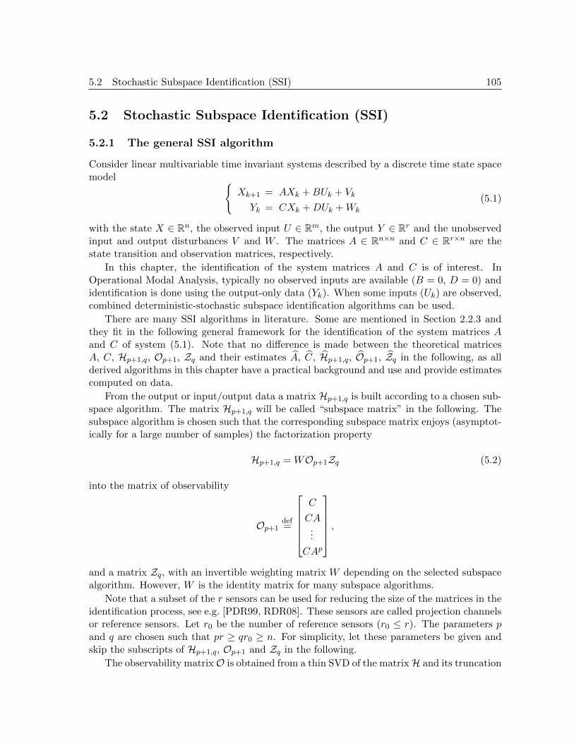
5.2 Stochastic Subspace Identification (SSI) 105
5.2 Stochastic Subspace Identification (SSI)
5.2.1 The general SSI algorithm
Consider linear multivariable time invariant systems described by a discrete time state spacemodel
Xk+1 = AXk +BUk + Vk
Yk = CXk +DUk +Wk
(5.1)
with the state X ∈ Rn, the observed input U ∈ Rm, the output Y ∈ Rr and the unobservedinput and output disturbances V and W . The matrices A ∈ Rn×n and C ∈ Rr×n are thestate transition and observation matrices, respectively.
In this chapter, the identification of the system matrices A and C is of interest. InOperational Modal Analysis, typically no observed inputs are available (B = 0, D = 0) andidentification is done using the output-only data (Yk). When some inputs (Uk) are observed,combined deterministic-stochastic subspace identification algorithms can be used.
There are many SSI algorithms in literature. Some are mentioned in Section 2.2.3 andthey fit in the following general framework for the identification of the system matrices Aand C of system (5.1). Note that no difference is made between the theoretical matricesA, C, Hp+1,q, Op+1, Zq and their estimates A, C, Hp+1,q, Op+1, Zq in the following, as allderived algorithms in this chapter have a practical background and use and provide estimatescomputed on data.
From the output or input/output data a matrix Hp+1,q is built according to a chosen sub-space algorithm. The matrix Hp+1,q will be called “subspace matrix” in the following. Thesubspace algorithm is chosen such that the corresponding subspace matrix enjoys (asymptot-ically for a large number of samples) the factorization property
Hp+1,q = WOp+1Zq (5.2)
into the matrix of observability
Op+1def=
C
CA...
CAp
,
and a matrix Zq, with an invertible weighting matrix W depending on the selected subspacealgorithm. However, W is the identity matrix for many subspace algorithms.
Note that a subset of the r sensors can be used for reducing the size of the matrices in theidentification process, see e.g. [PDR99, RDR08]. These sensors are called projection channelsor reference sensors. Let r0 be the number of reference sensors (r0 ≤ r). The parameters pand q are chosen such that pr ≥ qr0 ≥ n. For simplicity, let these parameters be given andskip the subscripts of Hp+1,q, Op+1 and Zq in the following.
The observability matrixO is obtained from a thin SVD of the matrixH and its truncation

106 Chapter 5
at the desired model order n:
H = U∆V T
=[U1 U0
] [∆1 0
0 ∆0
]V T , (5.3)
O = W−1U1∆1/21 . (5.4)
Note that the singular values in ∆1 are non-zero and O is of full column rank. The observationmatrix C is then found in the first block-row of the observability matrix O. The statetransition matrix A is obtained from the shift invariance property of O, namely as the leastsquares solution of
O↑A = O↓, where O↑ def=
C
CA...
CAp−1
, O↓ def
=
CA
CA2
...
CAp
. (5.5)
5.2.2 Multi-order SSI
In many practical applications the true system order n is unknown and it is common to dothe system identification for models (5.1) at different model orders n = nj , j = 1, . . . , t, with
1 ≤ n1 < n2 < . . . < nt ≤ minpr, qr0, (5.6)
and where t is the number of models to be estimated [PDR99, PDR01, VdAP04]. The choiceof the model orders nj , j = 1, . . . , t, is up to the user and also depends on the problem. Forexample, nj = j + c or nj = 2j + c with some constant c can be chosen. For example, thelatter makes sense for an application as in Section 5.5: There, the eigenvalues of the statetransition matrix are pairwise complex conjugate. Thus, two model orders are needed torecover one new mode.
The following notation for specifying these different model orders is used throughoutthis chapter. Let Oj ∈ R(p+1)r×nj , Aj ∈ Rnj×nj and Cj ∈ Rr×nj be the observability,state transition and observation matrix at model order nj , j ∈ 1, . . . , t, respectively. Let
furthermore be O↑j and O↓j the first respective last p block rows of Oj , analogously to thedefinition in (5.5).
Note that in Section 5.2.1 model order n was used, while from now on model orders nj will
be used. The matrices Aj , Cj , Oj , O↑j and O↓j fulfill the equations in Section 5.2.1, replacing
A, C, O, O↑ and O↓, as well as nj replaces n.
5.2.3 Computation of system matrices
The system matrix Aj is the solution of the least squares problem (5.5) at a chosen modelorder nj :
O↑jAj = O↓j . (5.7)

5.2 Stochastic Subspace Identification (SSI) 107
A numerically stable solution is
Aj = O↑j†O↓j , (5.8)
where † denotes the Moore-Penrose pseudoinverse. A more efficient and also numericallystable way to solve it [GVL96], uses the thin QR decomposition
O↑j = QjRj , (5.9)
where Qj ∈ Rpr×nj is a matrix with orthogonal columns and Rj ∈ Rnj×nj is upper triangular.Rj is assumed to be of full rank, which is reasonable as Oj is of full column rank. With
Sjdef= QTj O↓j , (5.10)
Sj ∈ Rnj×nj , the solution of the least squares problem is
Aj = R−1j Sj . (5.11)
The observation matrix Cj is found in the first block row of Oj .The conventional way to compute the system matrices Aj and Cj at the model orders nj ,
j = 1, . . . , t, is the following [PDR01]: First, the observability matrix Ot is computed at themaximal desired model order nt from (5.3)–(5.4). The observability matrix Oj at order njis obtained from the first nj columns of Ot. Then, the matrices Aj and Cj are the solutionof least squares problem (5.7) and the first block row of Oj , respectively. This approach issummarized in Algorithm 5.1, where the least squares solution is obtained either by usingthe pseudoinverse (5.8) or the QR decomposition with equations (5.9)–(5.11). Note that fora matrix X the matrix X[a1:a2,b1:b2] denotes the submatrix of matrix X containing the blockfrom rows a1 to a2 and columns b1 to b2 of matrix X.
Algorithm 5.1 Multi-order SSI
Input: Ot ∈ R(p+1)r×nt observability matrixn1, . . . , nt desired model orders satisfying (5.6)
1: for j = 1 to t do2: O↑j ←− Ot[1:pr,1:nj ], O
↓j ←− Ot[(pr+1):(p+1)r,1:nj ]
3: if method = pseudoinverse then
4: Aj ←− O↑j†O↓j
5: else if method = QR then6: QR decomposition O↑j = QjRj
7: Sj ←− QTj O↓j8: Aj ←− R−1j Sj9: end if
10: Cj ←− Ot[1:r,1:nj ]11: end forOutput: System matrices Aj , Cj at model orders n1, . . . , nt

108 Chapter 5
5.2.4 Computational complexities
In order to compare the performance of different algorithms for the multi-order computationof the system matrices Aj and Cj , j = 1, . . . , t, their number of floating point operations(flops) needs to be evaluated. Consider the observability matrix Ot at a maximal model
order nmaxdef= nt be given. As Cj is always a submatrix of Ot, only the computation of the
state transition matrices Aj is considered. For comparing different algorithms, the modelorders are assumed to be nj = j = 1, . . . , nmax. Note that all algorithms are derived forarbitrary model orders nj fulfilling (5.6).
The number of flops for an algorithm is determined for the computation of the systemmatrices at orders nj = 1, 2, . . . , n∗, where n∗ ≤ nmax. Thus, the complexity of an algorithmis indicated, where the choice of the parameters is influenced by the maximal model ordernmax and where the computation is stopped at a (possibly smaller) model order n∗. However,for a first evaluation, n∗ = nmax can be assumed.
The subspace matrix H is often of size (p + 1)r × qr0 and in practice it is set p + 1 = q
and nmax = qr0 [BBG+01]. Define cdef= pr/nmax and m
def= pr. Then, c ≈ r/r0 and hence
independent of p, q and nmax. Hence, the total flop count is a function of c, n∗ and nmax.Furthermore, use the simplifications
∑n∗j=1 j ≈ 1
2n2∗,
∑n∗j=1 j
2 ≈ 13n
3∗,
∑n∗j=1 j
3 ≈ 14n
4∗.
For example, the SVD needed for the pseudoinverse in (5.8) takes about 14mj2+8j3 flopsand the thin Householder QR decomposition (5.9) takes about 4mj2 − 4
3j3 flops [GVL96].
Accounting the necessary multiplications, the computation of Aj takes 16mj2 + 10j3 flops in(5.8) and 6mj2− 1
3j3 flops in (5.11). Accumulating the operations for model orders 1, . . . , n∗
and replacing m = cnmax leads to a total flop count of about 163 cnmaxn
3∗ + 5
2n4∗ flops using
the pseudoinverse and 2cnmaxn3∗ − 1
12n4∗ flops using the QR decomposition. Thus, the least
squares solution for the system matrix using the QR decomposition is favorable.
5.3 Fast algorithms for multi-order SSI
The computation of the system matrices at multiple orders is a big computational burden. Inthe previous section it was shown that the conventional algorithm for this task (Algorithm 5.1)has a computational complexity of O(n4max) for the identification of the system matrices atmodel orders 1, 2, . . . , nmax. In this section, efficient algorithms are derived for the multi-orderidentification of the system matrices, having a computational complexity of only O(n3max).
5.3.1 A first algorithm for fast multi-order computation of system matrices
Conventionally, the least squares problem for the state transition matrix Aj is solved at eachdesired model order nj = n1, . . . , nt. Now, an algorithm is derived that solves the leastsquares problem only once at the maximal desired model order nt (Equations (5.9) to (5.11)with j = t), leading to matrices Rt, St and At. Then, instead of solving the least squaresproblems at all the orders n1, . . . , nt−1, it is shown that the state transition matrices Aj atthese lower orders can be computed much more efficiently from submatrices of Rt and St,based on the following main theorem of this chapter.

5.3 Fast algorithms for multi-order SSI 109
Theorem 5.1 Let Ot, Qt, Rt and St be given at the maximal desired model order nt with
O↑t = QtRt, St = QTt O↓t , At = R−1t St, (5.12)
such that At is the least squares solution of
O↑tAt = O↓t .
Let j ∈ 1, . . . , t− 1, and let Rt and St be partitioned into blocks
Rt =
[R
(11)j R
(12)j
0 R(22)j
], St =
[S(11)j S
(12)j
S(21)j S
(22)j
], (5.13)
where R(11)j , S
(11)j ∈ Rnj×nj . Then, the state transition matrix Aj at model order nj, which
is the least squares solution of
O↑jAj = O↓j , (5.14)
satisfies
Aj = R(11)j−1S
(11)j . (5.15)
Proof: From (5.3) and (5.4) it follows that Oj consists of the first nj columns of Ot.This holds analogously for O↑j and O↓j . Hence, O↑t and O↓t can be partitioned into
O↑t =[O↑j O
↑j
], O↓t =
[O↓j O
↓j
], (5.16)
where O↑j and O↓j consist of the remaining columns of O↑t and O↓t . Let Qt be partitioned intothe blocks
Qt =[Q
(1)j Q
(2)j
], (5.17)
where Q(1)j ∈ Rpr×nj . From (5.12) and (5.17) follows
O↑t =[Q
(1)j Q
(2)j
] [R(11)j R
(12)j
0 R(22)j
]=[Q
(1)j R
(11)j B
](5.18)
with B = Q(1)j R
(12)j +Q
(2)j R
(22)j . Comparing (5.16) and (5.18), it follows
O↑j = Q(1)j R
(11)j , (5.19)
which obviously is a QR decomposition of O↑j . As Aj is the least squares solution of (5.14)and because of QR decomposition (5.19), Aj satisfies
Aj = R(11)j−1Q
(1)j
TO↓j . (5.20)

110 Chapter 5
Furthermore, from (5.12), (5.16) and (5.17) follows
St =
Q
(1)j
T
Q(2)j
T
[O↓j O
↓j
]=
Q
(1)j
TO↓j Q
(1)j
TO↓j
Q(2)j
TO↓j Q
(2)j
TO↓j
,
and comparing to (5.13) yields
S(11)j = Q
(1)j
TO↓j .
Plugging this into (5.20) leads to the assertion.
Hence, steps (5.9) and (5.10) for the least squares solution of the state transition matrixAj are not necessary anymore for j = 1, . . . , t− 1, and (5.11) is replaced by (5.15).
Furthermore, matrix R(11)j−1 is a submatrix of R−1t due to its triangular structure. Thus,
the inverse of Rt can be computed beforehand, avoiding the inversion of the matrices R(11)j
at each model order. The resulting algorithm for this fast multi-order computation of thesystem matrices is summarized in Algorithm 5.2.
Algorithm 5.2 Fast multi-order SSI – preliminary version
Input: Ot ∈ R(p+1)r×nt observability matrixn1, . . . , nt desired model orders satisfying (5.6)
1: O↑t ←− Ot[1:pr,1:nt], O↓t ←− Ot[(pr+1):(p+1)r,1:nt]
2: Ct ←− Ot[1:r,1:nt]3: QR decomposition O↑t = QtRt4: T ←− R−1t , St ←− QTt O↓t5: for j = 1 to t do6: Aj ←− T[1:nj ,1:nj ]St[1:nj ,1:nj ]7: Cj ←− Ct[1:r,1:nj ]8: end for
Output: System matrices Aj , Cj at model orders n1, . . . , nt
In Line 6 of Algorithm 5.2, Aj is computed as a matrix product with triangular matrixT[1:nj ,1:nj ] as one factor. This requires n3j flops, when T and St are known. However, com-
puting Aj = R−1t[1:nj ,1:nj ]St[1:nj ,1:nj ] by backward substitution, without computing R−1t[1:nj ,1:nj ]explicitly, has the same computational cost, when Rt and St are known. In this case, theinversion of Rt can be avoided, leading to a slightly more efficient algorithm. It is summarizedin Algorithm 5.3.
5.3.2 Fast iterative multi-order computation of system matrices
The fast multi-order computation of the state transition matrix from the previous sectioncan be further improved by expressing Aj+1 with the help of Aj , which reduces further thenumber of numerical operations.

5.3 Fast algorithms for multi-order SSI 111
Algorithm 5.3 Fast multi-order SSI
Input: Ot ∈ R(p+1)r×nt observability matrixn1, . . . , nt desired model orders satisfying (5.6)
1: O↑t ←− Ot[1:pr,1:nt], O↓t ←− Ot[(pr+1):(p+1)r,1:nt]
2: Ct ←− Ot[1:r,1:nt]3: QR decomposition O↑t = QtRt4: St ←− QTt O↓t5: for j = 1 to t do6: Aj ←− R−1t[1:nj ,1:nj ]St[1:nj ,1:nj ]7: Cj ←− Ct[1:r,1:nj ]8: end for
Output: System matrices Aj , Cj at model orders n1, . . . , nt
Corollary 5.2 Let Ot, Qt, Rt and St be given at the maximal desired model order nt. Definethe submatrices
R(11)j = Rt[1:nj ,1:nj ], S
(11)j = St[1:nj ,1:nj ],
R(12)j = Rt[1:nj ,(nj+1):nj+1], S
(12)j = St[1:nj ,(nj+1):nj+1],
R(22)j = Rt[(nj+1):nj+1,(nj+1):nj+1], S
(21)j = St[(nj+1):nj+1,1:nj ],
S(22)j = St[(nj+1):nj+1,(nj+1):nj+1],
(5.21)
and A1 = R(11)1−1S
(11)1 . Then it holds
Aj+1 =
[Aj R
(11)j−1S
(12)j
0 0
]+
[−R(11)
j−1R
(12)j R
(22)j−1
R(22)j−1
] [S(21)j S
(22)j
](5.22)
for j = 1, . . . , t− 1.
Proof: According to Theorem 5.1, above submatrices are defined such that Rj = R(11)j ,
Sj = S(11)j and
Rj+1 =
[R
(11)j R
(12)j
0 R(22)j
], Sj+1 =
[S(11)j S
(12)j
S(21)j S
(22)j
].
Then,
R−1j+1 =
[R
(11)j−1 −R(11)
j−1R
(12)j R
(22)j−1
0 R(22)j−1
].
Plugging this into Aj+1 = R−1j+1Sj+1, the assertion follows using Theorem 5.1 and replacing
Aj = R(11)j−1S
(11)j .
Hence, by using (5.22), the computation of Aj+1 needs about 4(nj+1 − nj)n2j+1 flops, if
Rt, St and Aj are known. Note that, again, no explicit inversion of matrix R(11)j is necessary.
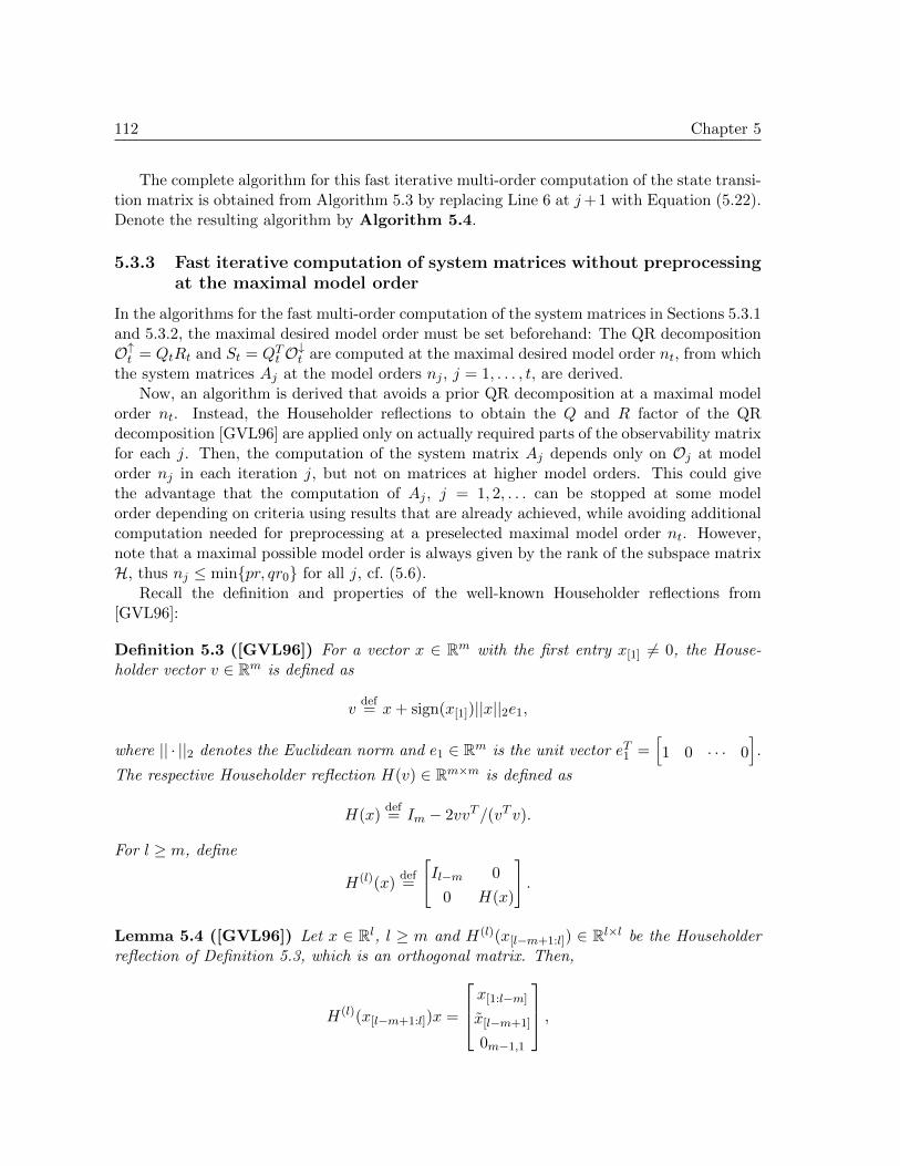
112 Chapter 5
The complete algorithm for this fast iterative multi-order computation of the state transi-tion matrix is obtained from Algorithm 5.3 by replacing Line 6 at j+1 with Equation (5.22).Denote the resulting algorithm by Algorithm 5.4.
5.3.3 Fast iterative computation of system matrices without preprocessingat the maximal model order
In the algorithms for the fast multi-order computation of the system matrices in Sections 5.3.1and 5.3.2, the maximal desired model order must be set beforehand: The QR decompositionO↑t = QtRt and St = QTt O↓t are computed at the maximal desired model order nt, from whichthe system matrices Aj at the model orders nj , j = 1, . . . , t, are derived.
Now, an algorithm is derived that avoids a prior QR decomposition at a maximal modelorder nt. Instead, the Householder reflections to obtain the Q and R factor of the QRdecomposition [GVL96] are applied only on actually required parts of the observability matrixfor each j. Then, the computation of the system matrix Aj depends only on Oj at modelorder nj in each iteration j, but not on matrices at higher model orders. This could givethe advantage that the computation of Aj , j = 1, 2, . . . can be stopped at some modelorder depending on criteria using results that are already achieved, while avoiding additionalcomputation needed for preprocessing at a preselected maximal model order nt. However,note that a maximal possible model order is always given by the rank of the subspace matrixH, thus nj ≤ minpr, qr0 for all j, cf. (5.6).
Recall the definition and properties of the well-known Householder reflections from[GVL96]:
Definition 5.3 ([GVL96]) For a vector x ∈ Rm with the first entry x[1] 6= 0, the House-holder vector v ∈ Rm is defined as
vdef= x+ sign(x[1])||x||2e1,
where || · ||2 denotes the Euclidean norm and e1 ∈ Rm is the unit vector eT1 =[1 0 · · · 0
].
The respective Householder reflection H(v) ∈ Rm×m is defined as
H(x)def= Im − 2vvT /(vT v).
For l ≥ m, define
H(l)(x)def=
[Il−m 0
0 H(x)
].
Lemma 5.4 ([GVL96]) Let x ∈ Rl, l ≥ m and H(l)(x[l−m+1:l]) ∈ Rl×l be the Householderreflection of Definition 5.3, which is an orthogonal matrix. Then,
H(l)(x[l−m+1:l])x =
x[1:l−m]
x[l−m+1]
0m−1,1
,

5.3 Fast algorithms for multi-order SSI 113
where x[l−m+1] is an entry changed by the Householder reflection and 0a,b is a matrix of size
a× b containing zeros. The multiplication of H(l)(x[l−m+1:l]) with an arbitrary vector can be
done with about 4m flops, without computing H(l)(x[l−m+1:l]) explicitly.
For X ∈ Rl×k, l ≥ m ≥ k, define the matrix H(l)(X[l−m+1:l,1:k]) ∈ Rl×l as a product ofHouseholder reflections, such that
H(l)(X[l−m+1:l,1:k])X =
X[1:l−m,1:k]
X
0m−k,k
,
where X ∈ Rk×k is an upper triangular matrix resulting from the Householder reflections.The multiplication of H(l)(X[l−m+1:l,1:k]) with an arbitrary vector can be done with about
2k(2m− k) flops, without computing H(l)(X[l−m+1:l,1:k]) explicitly.
With these definitions, the Householder reflections that are necessary to get the leastsquares solution for the system matrices can be applied stepwise on the appropriate parts ofthe observability matrix. Thus, the explicit computation of the factor Q of a QR decompo-sition is not necessary anymore.
Proposition 5.5 Let the observability matrices O1,O2, . . . at model orders n1 < n2 < . . . begiven. Define H1 = H(pr)(O↑1), R1 = H1O↑1 and S1 = H1O↓1. For j = 1, 2, . . . define oj+1
such thatOj+1 =
[Oj oj+1
].
ando↑j+1 = Hj · · ·H1o
↑j+1, o↓j+1 = Hj · · ·H1o
↓j+1. (5.23)
Let Hj+1def= H(pr)(o↑j+1[(nj+1):pr,1:(nj+1−nj)]) be a collection of Householder reflections and
define
Rj+1 =[Rj Hj+1o
↑j+1
], Sj+1 = Hj+1
[Sj o↓j+1
]. (5.24)
Then, the solution of the least squares problem O↑j+1Aj+1 = O↓j+1 is given by
Aj+1 = (Rj+1[1:nj+1,1:nj+1])−1Sj+1[1:nj+1,1:nj+1].
Proof: As Rj is by construction an upper triangular matrix with Rj[(nj+1):pr,1:nj ] = 0,
it follows Hj+1Rj = Rj from the definition of Hj+1. Then, from (5.24) follows Rj+1 =
Hj+1
[Rj o↑j+1
]and together with (5.24), it follows
Rj+1 = Hj+1
[Rj o↑j+1
]= Hj+1
[Hj
[Rj−1 o↑j
]o↑j+1
]
= Hj+1Hj
[Rj−1 Hj−1 · · ·H1
[o↑j o↑j+1
]]= . . .
= Hj+1Hj · · ·H1
[O↑1 o↑2 . . . o↑j+1
]
= Hj+1Hj · · ·H1O↑j+1.

114 Chapter 5
Analogously, it holds Sj+1 = Hj+1Hj · · ·H1O↓j+1. The Householder reflections were
chosen such that Rj+1 ∈ Rpr×nj+1 is upper triangular. Hence, O↑j+1 = Qj+1Rj+1 with
QTj+1 = Hj+1Hj · · ·H1 ∈ Rpr×pr is a full QR decomposition of O↑j+1 and Sj+1 = QTj+1O↓j+1.Thus, the assertion follows.
With this proposition, the matrices Rj+1 and Sj+1 are computed iteratively. Then, Corol-lary 5.2 can be used to compute Aj+1 at each iteration efficiently, using Rj+1 and Sj+1 insteadof Rt and St, respectively. For the latter operation, about 4(nj+1−nj)n2j+1 flops are necessary
at the model order nj+1, as stated in the previous section. For the computation of Rj+1 andSj+1, 2
∑njk=1 4(pr−k)(nj+1−nj) ≈ (8prnj−4n2j )(nj+1−nj) flops are necessary for (5.23) and∑nj+1
k=nj+1 4(pr− k)(nj+1 − nj + nj+1) ≈ (4prnj+1 − 4n2j+1)(nj+1 − nj) flops are necessary for
(5.24). Thus, at each model order nj+1 a total number of about (12prnj+1−4n2j+1)(nj+1−nj)flops is necessary to compute Aj+1.
The complete algorithm for this fast iterative multi-order computation of the state transi-tion matrix is obtained from Algorithm 5.3 by replacing Line 6 at j+1 with Equation (5.22),while replacing Rt and St in (5.21) by Rj+1 and Sj+1 from (5.24). Denote the resultingalgorithm by Algorithm 5.5.
5.3.4 Comparison of multi-order algorithms
The computational complexities for the computation of the system matrices with the multi-order SSI algorithms from the last sections are summarized in Table 5.1. All results aregiven for the computation at model orders 1, 2, . . . , n∗ from an observability matrix of size(cnmax + r)× nmax, where n∗ ≤ nmax.
The conventional Algorithm 5.1, either using the pseudoinverse or the QR decompositionfor the solution of the least squares problem, takes O(n4max) operations for n∗ = nmax. Thesimplest of the derived fast algorithms, Algorithms 5.2 and 5.3, are still dependent on n4∗,although its constant is significantly smaller than for Algorithm 5.1, and even (6 c− 4
3)n3max ≥14 n
4∗ in many cases. Algorithm 5.3 has a slight advantage over Algorithm 5.2.
Table 5.1 – Computational complexities of multi-order system matrix identification from SSI.
Algorithm Flops
SSI with pseudoinverse (Algorithm 5.1) 163 cnmaxn
3∗ + 5
2n4∗
SSI with QR (Algorithm 5.1) 2cnmaxn3∗ − 1
12n4∗
Fast SSI (Algorithm 5.2) (6c− 1)n3max + 14n
4∗
Fast SSI (Algorithm 5.3) (6c− 43)n3max + 1
4n4∗
Iterative Fast SSI (Algorithm 5.4) (6c− 43)n3max + 4
3n3∗
Iterative Fast SSI (Algorithm 5.5) 6cnmaxn2∗ − 4
3n3∗

5.4 Eigensystem Realization Algorithm (ERA) 115
Finally, the iterative fast SSI algorithms from Sections 5.3.2 and 5.3.3 (Algorithms 5.4and 5.5) take only O(n3max) operations for n∗ = nmax. However, even if Algorithm 5.5 needsthe least number of operations, it is rather of theoretical value, as a practical implementationis cumbersome. Furthermore, Algorithm 5.5 might perform less well in practice due to themanual handling of matrix operations.
5.3.5 Iterative computation of Rt and St
In the Algorithms 5.2–5.4 the matrices Rt and St are computed from Ot at the maximaldesired model order nt. From these matrices, the state transition matrix Aj is derived atinferior model orders nj , j = 1, . . . , t.
However, Ot can be a very large matrix with (p + 1)r nt, for example in the caseof a large number of sensors r or using multiple sensor setups as in Chapter 4. Then, thecomputation of Rt and St could pose a memory problem. In this case, the matrices Rtand St can be computed iteratively by cutting Ot in block rows and using an iterative QRdecomposition. This solves the possible memory problem as Rt and St are only of size nt×nt.The iterative computation of Rt and St was already detailed in Propositions 3.8 and 4.5. It
can be applied to any separation of Ot into block rows O(0)t , . . . ,O(J)
t , where each block O(j)t
relates to a sensor set defined by partial observation matrices C(j)t , j = 0, . . . , J , such that
the observation matrix Ct writes
Ct =
C(0)t
C(1)t...
C(J)t
, and Ot =
O(0)t
O(1)t...
O(J)t
with O(j)t =
C(j)t
C(j)t At
...
C(j)t Apt
for j = 0, . . . , J . Thus, Rt and St can be obtained iteratively from the blocks O(0)t , . . . ,O(J)
t .Then, the estimates of the state transition matrices Aj at model orders nj , j = 1, . . . , t canbe obtained from Rt and St by one of the Algorithms 5.2–5.4. Estimates of Cj are obtainedfrom Ct.
5.4 Eigensystem Realization Algorithm (ERA)
5.4.1 System identification with ERA
System identification with NExT-ERA is closely related to covariance-driven stochastic sub-space identification. The Natural Excitation Technique (NExT) [JICL95, FJI97] states thatthe cross-correlation function between two responses made on unknown ambient excitationhas the same form as the system’s impulse response function under convenient assumptions.Then, the Eigensystem Realization Algorithm (ERA) [JP85], which was developed to analyzeimpulse response functions, can be applied for system identification.
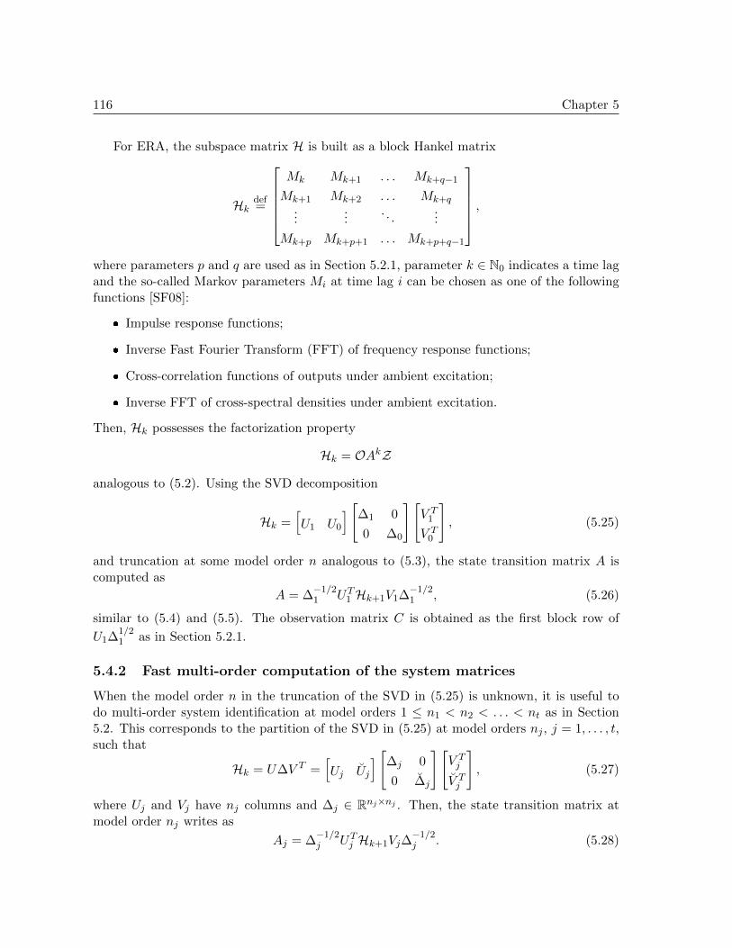
116 Chapter 5
For ERA, the subspace matrix H is built as a block Hankel matrix
Hk def=
Mk Mk+1 . . . Mk+q−1
Mk+1 Mk+2 . . . Mk+q...
.... . .
...
Mk+p Mk+p+1 . . . Mk+p+q−1
,
where parameters p and q are used as in Section 5.2.1, parameter k ∈ N0 indicates a time lagand the so-called Markov parameters Mi at time lag i can be chosen as one of the followingfunctions [SF08]:
Impulse response functions;
Inverse Fast Fourier Transform (FFT) of frequency response functions;
Cross-correlation functions of outputs under ambient excitation;
Inverse FFT of cross-spectral densities under ambient excitation.
Then, Hk possesses the factorization property
Hk = OAkZ
analogous to (5.2). Using the SVD decomposition
Hk =[U1 U0
] [∆1 0
0 ∆0
][V T1
V T0
], (5.25)
and truncation at some model order n analogous to (5.3), the state transition matrix A iscomputed as
A = ∆−1/21 UT1 Hk+1V1∆
−1/21 , (5.26)
similar to (5.4) and (5.5). The observation matrix C is obtained as the first block row of
U1∆1/21 as in Section 5.2.1.
5.4.2 Fast multi-order computation of the system matrices
When the model order n in the truncation of the SVD in (5.25) is unknown, it is useful todo multi-order system identification at model orders 1 ≤ n1 < n2 < . . . < nt as in Section5.2. This corresponds to the partition of the SVD in (5.25) at model orders nj , j = 1, . . . , t,such that
Hk = U∆V T =[Uj Uj
] [∆j 0
0 ∆j
][V Tj
V Tj
], (5.27)
where Uj and Vj have nj columns and ∆j ∈ Rnj×nj . Then, the state transition matrix atmodel order nj writes as
Aj = ∆−1/2j UTj Hk+1Vj∆
−1/2j . (5.28)

5.4 Eigensystem Realization Algorithm (ERA) 117
Proposition 5.6 Let At from (5.27) and (5.28) at a maximal desired model order nt begiven. Then, Aj satisfying (5.28) at model order nj is a submatrix of At and fulfills
Aj = At[1:nj ,1:nj ].
Proof: From (5.27) and (5.28), At is defined as
At = ∆−1/2t UTt Hk+1Vt∆
−1/2t .
For any j = 1, . . . , t, it holds by definition
Ut =[Uj Uj
], ∆
−1/2t =
[∆−1/2j 0
0 ∆−1/2j
], Vt =
[Vj Vj
]
with some matrices Uj , ∆j and Vj . Thus, plugging this in the definition of At it follows
At =
[∆−1/2j UTj Hk+1Vj∆
−1/2j ∆
−1/2j UTj Hk+1Vj∆
−1/2j
∆−1/2j UTj Hk+1Vj∆
−1/2j ∆
−1/2j UTj Hk+1Vj∆
−1/2j
]
and comparing with the definition of Aj in (5.28), the assertion follows.
Hence, for multi-order system identification with ERA, only At at the maximal desiredmodel order nt needs to be computed. Then, the matrices Aj , j = 1, . . . , t − 1, are simplysubmatrices of At and do not require further computations.
With the following corollary, the prior computation of At at the maximal desired modelorder nt can be avoided and the matrices Aj are defined iteratively, analogous to Section5.3.3.
Corollary 5.7 Let Hk, Hk+1 and the SVD (5.27) be given. Define T1 = ∆−1/21 UT1 Hk+1 and
A1 = T1V1∆−1/21 . For j = 1, 2, . . . define uj+1, σj+1 and vj+1 such that
Uj+1 =[Uj uj+1
], ∆j+1 =
[∆j 0
0 σj+1
], Vj+1 =
[Vj vj+1
],
and
tj+1 = σ−1/2j+1 u
Tj+1Hk+1, Tj+1 =
[Tj
tj+1
]. (5.29)
Then,
Aj+1 =
[Aj Tjvj+1σ
−1/2j+1
tj+1Vj∆−1/2j tj+1vj+1σ
−1/2j+1
]. (5.30)
Proof: Replace At, Ut, ∆t and Vt in the proof of Proposition 5.6 by Aj+1, Uj+1, ∆j+1
and Vj+1.

118 Chapter 5
For a comparison of the computational complexity of this algorithm with the results ofSection 5.3.4, it is assumed that the SVD (5.27) is the starting point of the computation,which is analogous to assume that the observability matrix used for SSI algorithms is alreadyknown. The notation of Sections 5.2.4 and 5.3.4 is used and Hk is assumed to be of sizecnmax × nmax.
About (2c + 2)n3max flops are necessary to compute At at model order nt = nmax, fromwhich the state transition matrices at inferior orders are selected in Proposition 5.6. InCorollary 5.7, the computation of Aj at some order j takes about 2cn2max + 4nmaxj flops,amounting to 2cn2maxn∗+ 2nmaxn
2∗ flops when computing at all orders 1, 2, . . . , n∗. Note that
the conventional computation of Aj for all j = 1, . . . , t from (5.28) needs about (12c + 12)n4∗
flops.
The computational complexities of the derived multi-order ERA algorithms are summa-rized in Table 5.2.
Table 5.2 – Computational complexities of multi-order system matrix identification from ERA.
Algorithm Flops
Conventional Computation (12c+ 12)n4∗
Fast Computation (Proposition 5.6) (2c+ 2)n3max
Iterative Fast Computation (Corollary 5.7) 2cn2maxn∗ + 2nmaxn2∗
5.5 Structural vibration analysis example
In this section, the fast multi-order computation of the system matrices is applied to a prac-tical test case from vibration analysis. In Section 2.4, the underlying mechanical model andits respective discrete time state-space model were recalled. For eigenstructure identification,so-called stabilization diagrams (cf. Section 2.4.3) are used that contain the system identifi-cation results at multiple model orders. At each of these model orders, the system matriceshave to be computed first in order to get the eigenstructure of the respective systems. Forsystem identification with SSI algorithms or with ERA, this can be done efficiently and fastwith the new algorithms derived in this chapter.
5.5.1 Numerical results of multi-order system identification
All system identification algorithms of this chapter are applied to the system identificationof the Z24 Bridge [MDR03, Par03] as in Section 4.7. It was a prestressed concrete bridgewith three spans, supported by two intermediate piers and a set of three columns at eachend. Both types of supports are rotated with respect to the longitudinal axis which resultsin a skew bridge. The overall length is 58 m.
The ambient vibration data was measured in nine setups of up to 33 sensors each, withfive reference sensors common to all setups. Altogether, the structure was measured at

5.5 Structural vibration analysis example 119
r = 251 sensor positions, of which are r0 = 5 reference sensors. In each setup, 65,536 sampleswere collected for each sensor with a sampling frequency of 100 Hz. The common subspacematrix of all setups was obtained with the merging approach described in Chapter 4 usingdata-driven SSI with the Unweighted Principal Component Algorithm.
The different algorithms presented in this chapter are tested on an Intel Xeon CPU 3.40GHz with 16 GByte in Matlab 7.10.0.499 using one processor kernel. With these algorithms,the system matrices Aj and Cj are computed at model orders nj = 1, 2, . . . , nmax. Fromthese results, the modal parameters of the system can be identified using the stabilizationdiagram. To compare the performance of the algorithms, the system matrices are computedfor stabilization diagrams with different maximal model orders nmax.
For SSI algorithms, a subspace matrix H of size (p + 1)r × qr0 is built from the data,where p + 1 = q is chosen, as recommended in [BBG+01]. Ot is obtained from H,where the maximal model order is nmax = nt = qr0. Then, the time is recorded for thecomputation of Aj and Cj from Ot at model orders nj = j = 1, 2, . . . , nmax.
For ERA, the matrix H from the subspace algorithm is used for simplicity. Setnmax = qr0, Hk = H[1:pr,1:qr0] and Hk+1 = H[(r+1):(p+1)r,1:qr0]. Then, the SVD ofHk is performed and the time is recorded for the computation of Aj and Cj from U ,∆, V and Hk+1 at model orders nj = j = 1, 2, . . . , nmax.
To evaluate the computational time for obtaining the set of Aj ’s and Cj ’s from order 1 untila maximal model order nmax = qr0, these steps are repeated for q = 2, . . . , 100. As thecomputation time is also dependent on the constant c ≈ r/r0 (see Section 5.2.4), first acomputation is done with all r = 251 sensors (c ≈ 50), and second a computation with onlya subset of r = 5 sensors (c ≈ 1).
5.5.1.1 Computation times of multi-order SSI algorithms at different maximalmodel orders
The computation times for the computation of the system matrices at model orders1, 2, . . . , nmax from an observability matrix Onmax with the SSI algorithms are presentedin Figure 5.1 for different maximal model orders nmax. It can be seen that the solution ofthe least squares problem with the QR decomposition is more efficient than using the pseu-doinverse in the conventional Algorithm 5.1, as expected. The Algorithms 5.2–5.4 derivedin this chapter yield a significant reduction in the computation times. Although Algorithm5.5 theoretically needs the least number of operations, it does not perform well in practice,which is already explained in Section 5.3.4. Besides the latter algorithm, all other algorithmsseem to be consistent with their theoretical performance.
At each maximal model order, the computation time in Figure 5.1 corresponds to thetotal time that is needed to compute all the system matrices for a stabilization diagramhaving this maximal model order. It is clearly shown that the new fast iterative multi-orderSSI with Algorithm 5.4 outperforms the other algorithms. For nmax = 500 it takes a total of13.7 s, while the conventional multi-order Algorithm 5.1 using the pseudoinverse takes 2873 s,thus being more than 200 times faster.

120 Chapter 5
0 50 100 150 200 250 300 350 400 450 50010
−3
10−2
10−1
100
101
102
103
104
maximal model order nmax
com
puta
tiona
l tim
e (s
)
conventional SSI with pseudoinverse (Alg. 5.1)conventional SSI with QR (Alg. 5.1)fast SSI (Alg. 5.2)fast SSI (Alg. 5.3)iterative fast SSI (Alg. 5.4)iterative fast SSI / Householder (Alg. 5.5)
(a) r = 251, r0 = 5, c ≈ 50
0 50 100 150 200 250 300 350 400 450 50010
−4
10−3
10−2
10−1
100
101
102
103
maximal model order nmax
com
puta
tiona
l tim
e (s
)
conventional SSI with pseudoinverse (Alg. 5.1)conventional SSI with QR (Alg. 5.1)fast SSI (Alg. 5.2)fast SSI (Alg. 5.3)iterative fast SSI (Alg. 5.4)iterative fast SSI / Householder (Alg. 5.5)
(b) r = r0 = 5, c ≈ 1
Figure 5.1 – Computation times for multi-order SSI system identification of system matrices Aj and Cj , nj = j =1, . . . , nmax from Onmax at different maximal model orders nmax.
5.5.1.2 Computation times of multi-order SSI algorithms for maximal modelorder 500
The accumulated computation times of the system matrices at model orders 1, 2, . . . , n∗ forthe maximal model order nmax = 500 are presented in Figure 5.2 for n∗ = 1, . . . , 500. Thiscorresponds to the time that is needed to compute the system matrices up to each order n∗for a stabilization diagram of maximal model order nmax = 500.
Due to a preprocessing step at the maximal model order in Algorithms 5.2–5.4, the
0 50 100 150 200 250 300 350 400 450 50010
−1
100
101
102
103
104
model order n*
accu
mul
ated
com
puta
tiona
l tim
e (s
)
conventional SSI with pseudoinverse (Alg. 5.1)conventional SSI with QR (Alg. 5.1)fast SSI (Alg. 5.2)fast SSI (Alg. 5.3)iterative fast SSI (Alg. 5.4)iterative fast SSI / Householder (Alg. 5.5)
(a) r = 251, r0 = 5, c ≈ 50
0 50 100 150 200 250 300 350 400 450 50010
−3
10−2
10−1
100
101
102
103
model order n*
accu
mul
ated
com
puta
tiona
l tim
e (s
)
conventional SSI with pseudoinverse (Alg. 5.1)conventional SSI with QR (Alg. 5.1)fast SSI (Alg. 5.2)fast SSI (Alg. 5.3)iterative fast SSI (Alg. 5.4)iterative fast SSI / Householder (Alg. 5.5)
(b) r = r0 = 5, c ≈ 1
Figure 5.2 – Accumulated computation times for multi-order SSI system identification up to different model ordersn∗ with maximal model order nmax = 500.

5.5 Structural vibration analysis example 121
accumulated computation time for the first model orders n∗ is higher in these fast algorithmsthan for the conventional algorithms. However, this changes quickly at higher model ordersand the new algorithms outperform the conventional ones, with Algorithm 5.4 being thefastest. It is also noted that the preprocessing step takes the main part of the computation,while after that, the computation of the system matrices at all orders 1, 2, . . . , 500 take onlyabout 2.4 seconds for Algorithm 5.4 in Figures 5.2(a) and 5.2(b).
5.5.1.3 Computation times of multi-order ERA algorithms
The computation times for the computation of the system matrices at model orders1, 2, . . . , nmax from an observability matrix Onmax with the ERA algorithms are presentedin Figure 5.3 for different maximal model orders nmax. The accumulated computation timesof the system matrices at model orders 1, 2, . . . , n∗ for the maximal model order nmax = 500are presented in Figure 5.4 for n∗ = 1, . . . , 500.
From both figures it can be seen that the new multi-order algorithms for ERA developedin this chapter are significantly faster than the conventional ERA algorithm. Due to its im-plementation, the fast ERA algorithm from Proposition 5.6 outperforms its iterative variantfrom Corollary 5.7, except when stopping the computation at a low model order. For thecomputation of the system matrices at orders 1, 2, . . . , 500 with nmax = 500, the fast multi-order ERA algorithm takes a total of 5 s, while the conventional multi-order ERA algorithmtakes 980 s, thus being about 200 times faster.
0 50 100 150 200 250 300 350 400 450 50010
−4
10−3
10−2
10−1
100
101
102
103
104
maximal model order nmax
com
puta
tiona
l tim
e (s
)
conventional ERAfast ERA (Prop. 5.6)iterative fast ERA (Cor. 5.7)
Figure 5.3 – Computation times for multi-order ERAsystem identification of system matrices Aj and Cj ,nj = j = 1, . . . , nmax from Onmax at different maximalmodel orders nmax with r = 251, r0 = 5, c ≈ 50.
0 50 100 150 200 250 300 350 400 450 50010
−2
10−1
100
101
102
103
104
model order n*
accu
mul
ated
com
puta
tiona
l tim
e (s
)
conventional ERAfast ERA (Prop. 5.6)iterative fast ERA (Cor. 5.7)
Figure 5.4 – Accumulated computation times for multi-order ERA system identification up to different modelorders n∗ with maximal model order nmax = 500 andr = 251, r0 = 5, c ≈ 50.
5.5.1.4 Discussion of the results
In Figure 5.1, computation times are obtained for multi-order system identification with SSIfor different maximal model orders, where for each maximal order nmax the system matricesare computed at orders 1, 2, . . . , nmax. In Figure 5.2, the accumulated computation times at

122 Chapter 5
each of these orders 1, 2, . . . , nmax are obtained for nmax = 500. With these results, the perfor-mance of the algorithms proposed in this chapter can be evaluated for the computation of thesystem matrices up to a maximal model order nmax as well as up to a lower order n∗ ≤ nmax.From both figures it can be seen that the conventional algorithm (Algorithm 5.1 using thepseudoinverse), which is widely used, is the slowest except when stopping the computation ata very small model order. Using the QR decomposition in Algorithm 5.1 yields already fasterresults, while the new Algorithms 5.2–5.4 yield significant improvements in the computationtime. Algorithm 5.2 yields slightly slower results than Algorithm 5.3. Algorithm 5.4 is ingeneral the fastest of these algorithms, except at very low model orders, where computationtimes are lower than 0.01 s. Algorithm 5.5 theoretically needs even less operations (cf. Table5.1), but is in practice slower due to its implementation. As the theoretical performances ofAlgorithms 5.4 and 5.5 are very close, Algorithm 5.4 is favorable.
In Figures 5.3 and 5.4 corresponding results for the ERA algorithms from Section 5.4are obtained. Although the fast multi-order computation (Proposition 5.6) and its iterativevariant (Corollary 5.7) theoretically need the same number of operations for n∗ = nmax inFigure 5.3, the former algorithm is faster due to implementation reasons. When stoppingthe computation at lower model orders in Figure 5.4, the iterative algorithm is faster only atvery low model orders. In both cases, the conventional multi-order algorithm is the slowest.
5.5.2 Modal parameter estimation and stabilization diagram
In order to obtain the modal parameters of the vibration analysis example (cf. Section 2.4),the multi-order system identification performed in the previous section is one part of thetask. From these results, the eigenstructure of the investigated structure is obtained fromthe system matrices at the multiple orders using (2.55) and (2.56) in the next step. Note that
Frequency
302520151050
200
150
100
50
Model order
Stabilization diagram
Figure 5.5 – Stabilization diagram of Z24 Bridge containing the identified natural frequencies at model orders1, . . . , 250 using the fast iterative SSI (Algorithm 5.4).

5.7 Dissemination 123
the eigenstructure computation has a complexity of O(n3j ) at each model order nj and thus
O(n4max) for the entire computation. However, for nmax = 500 this step took a total time of168 s, thus being a small part compared to the conventional multi-order system identificationalgorithms. It is beyond the scope of this chapter to optimize this process.
A stabilization diagram containing the natural frequencies of the Z24 Bridge at modelorders 1, . . . , 250 is presented in Figure 5.5. Note that some of the modes – the ones that mightnot be very well excited – stabilize late in the diagram, making it necessary to use high modelorders for system identification. Using even higher model orders than 250 can still improvethe identification results, although there are only 10 modes present in this case [Par03].
5.6 Conclusions
In this chapter, new algorithms were derived to efficiently compute the system matricesat multiple model orders in stochastic subspace-based system identification (SSI) and theclosely related Eigensystem Realization Algorithm (ERA). The computational complexityfor this task was reduced from O(n4max) to O(n3max), where nmax is the maximal desiredmodel order. These algorithms are especially applied in the modal analysis of mechanical,civil or aeronautical structures, where eigenstructure identification results at multiple modelorders are used to distinguish physical from spurious modes using stabilization diagrams.
The efficiency of the new algorithms was shown on a real test case and computation timewas reduced up to a factor of 200 and more. These fast algorithms can e.g. be exploited inonline monitoring, where incoming data has to be processed quickly.
5.7 Dissemination
Parts of this chapter have been published or are submitted to:
[DM11a] M. Dohler and L. Mevel. Fast multi-order stochastic subspace-based systemidentification. 2011. Control Engineering Practice, under revision.
[DM11b] M. Dohler and L. Mevel. Fast multi-order stochastic subspace identification.In Proc. 18th IFAC World Congress, Milan, Italy, 2011.
The fast multi-order identification algorithms have been transferred to the commercialsoftware product ARTeMIS Extractor Pro [Str11].

124 Chapter 5

Part III
Fault detection
125


Chapter 6
Robust subspace-based faultdetection under changing excitation
6.1 Introduction
Subspace methods enjoy some popularity, especially in vibration analysis of civil, aeronauticalor mechanical structures, where large model orders have to be considered. The excitation isambient and mostly unmeasured. In most cases it is impractical to use artificial excitationsources, such as shakers, where a part of the excitation is measured. Details of the modelingof the underlying mechanical system are found in Section 2.4.
In the last twenty years, monitoring the integrity of the civil infrastructure has been anactive research topic, including in connected areas such as automatic control, for masteringthe aging of bridges, or the resistance to seismic events and the protection of the culturalheritage. It is assumed that changes in the structural properties lead to changes in theeigenstructure of a system.
In order to detect changes in the modal parameters linked to the structural parameters,often eigenstructure identification results are used and evaluated for changes, e.g. [Kul03,MaCC08, MaCC10, RML+10]. The modal parameters are not afflicted by different ambientexcitations, but their automatic estimation and matching from measurements of differentstates of the structure might require an extensive preprocessing step.
A subspace-based residual function that is robust to excitation change is considered in[YG06]. Recently, a modified whiteness test for damage detection, which is is robust tochanges in the excitation, was proposed in [BB11, Ber11b] using Kalman filter innovations.
In this chapter, the subspace-based fault detection approach from [BAB97, BAB00,BMG04] is considered. It uses a subspace-based residual built on the left null space of anominal observability matrix of the system in a reference state, which is the same as thecorresponding subspace matrix built from the output data. In a possibly damaged state it is

128 Chapter 6
then checked, whether the corresponding subspace matrix is still well described by the nullspace of the reference state, using a χ2-test on the residual. The statistical theory behindthe χ2-test and the subspace-based fault detection are explained in detail in Section 2.3.
However, the subspace matrix is influenced by the properties of the unmeasured ambientexcitation. Most works on the subspace-based fault detection test assume that these proper-ties stay constant between measurements of the investigated structure in the reference andpossibly damaged condition, which is hardly the case for real applications. Robustness tonon-stationary excitation within one measurement has already been addressed in [MB86].We assume stationary excitation during one measurement, while the excitation covariancemay change between measurements. In this chapter, the problem of robustness to changesin the excitation of this fault detection method is addressed. Two modifications of the faultdetection test are proposed to make it robust to excitation changes.
After recalling the basic principles of subspace-based system identification and statisticalfault detection in Section 6.2, the impact of a changing ambient excitation between mea-surements on the fault detection test is discussed in Section 6.3. Using strategies for thenormalization of the subspace matrices with respect to different excitations of Chapter 4, afirst modification of the test is proposed in Section 6.4. A more general approach for ro-bustness to changing excitation is proposed in Section 6.5, where a robust residual functionand its corresponding χ2-test are derived. In Section 6.6, numerical results of the proposedalgorithms are presented.
6.2 Statistical subspace-based fault detection
In Sections 6.2.1 and 6.2.2 the basic concepts of stochastic subspace-based system identi-fication and fault detection are recalled from Chapter 2 and generalized to SSI algorithmswithout a left weighting matrix.
6.2.1 General SSI algorithm
Consider the discrete time model in state space form:
Xk+1 = AXk + Vk
Yk = CXk
(6.1)
with the state X ∈ Rn, the output Y ∈ Rr, the state transition matrix A ∈ Rn×n and theobservation matrix C ∈ Rr×n. The excitation (Vk)k is an unmeasured Gaussian white noise
sequence with zero mean and constant covariance matrix Q: E(VkVTk′ )
def= Qδ(k − k′), where
E(·) denotes the expectation operator.
A subset of the r sensors may be used for reducing the size of the matrices in the identi-fication process. These sensors are called projection channels or reference sensors. Let r0 bethe number of reference sensors (r0 ≤ r) and p and q chosen parameters with pr ≥ qr0 ≥ n.
Denote a matrix Hp+1,q ∈ R(p+1)r×qr0 as subspace matrix, whose estimate Hp+1,q is builtfrom the output data (Yk)k=1,...,N+p+q according to a chosen SSI algorithm. In this chapter,

6.2 Statistical subspace-based fault detection 129
only SSI algorithms without a left weighting matrix are considered. The subspace matrixenjoys the factorization property
Hp+1,q = Op+1Zq (6.2)
into the matrix of observability
Op+1 =
C
CA...
CAp
and a matrix Zq depending on the selected SSI algorithm. The observation matrix C is thenfound in the first block-row of the observability matrix Op+1. The state transition matrix A isobtained from the shift invariance property of Op+1 and the eigenstructure (λ, ϕλ) of system(6.1) results from
det(A− λI) = 0, Aφλ = λφλ, ϕλ = Cφλ,
where λ ranges over the set of eigenvalues of A. The collection of modes and mode shapes(λ, ϕλ) is a canonical parameterization of system (6.1) and considered as the system parameterθ with
θdef=
[Λ
vec Φ
], (6.3)
where Λ is the vector whose elements are the eigenvalues λ and Φ is the matrix whose columnsare the mode shapes ϕ.
The actual implementation of this generic subspace identification algorithm uses a con-sistent estimate Hp+1,q obtained from the output data according to the selected subspaceidentification algorithm. The SVD
Hp+1,q =[U1 U0
] [∆1 0
0 ∆0
][V T1
V T0
](6.4)
and its truncation at the model order n yields an estimate
Op+1 = U1∆1/21
for the observability matrix, from which (C, A) and (λ, ϕλ) are recovered as sketched above.Note that the singular values in ∆1 are non-zero and Op+1 is of full column rank. Thematrices
U1 =[u1 . . . un
], V1 =
[v1 . . . vn
], ∆1 = diagσ1, . . . , σn (6.5)
contain the first n left and right singular vectors, and singular values of Hp+1,q.
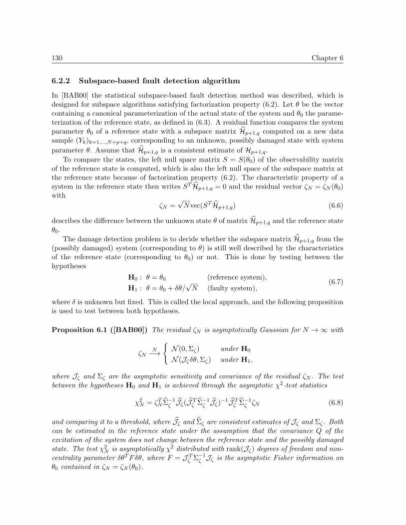
130 Chapter 6
6.2.2 Subspace-based fault detection algorithm
In [BAB00] the statistical subspace-based fault detection method was described, which isdesigned for subspace algorithms satisfying factorization property (6.2). Let θ be the vectorcontaining a canonical parameterization of the actual state of the system and θ0 the parame-terization of the reference state, as defined in (6.3). A residual function compares the systemparameter θ0 of a reference state with a subspace matrix Hp+1,q computed on a new datasample (Yk)k=1,...,N+p+q, corresponding to an unknown, possibly damaged state with system
parameter θ. Assume that Hp+1,q is a consistent estimate of Hp+1,q.
To compare the states, the left null space matrix S = S(θ0) of the observability matrixof the reference state is computed, which is also the left null space of the subspace matrix atthe reference state because of factorization property (6.2). The characteristic property of asystem in the reference state then writes ST Hp+1,q = 0 and the residual vector ζN = ζN (θ0)with
ζN =√Nvec(ST Hp+1,q) (6.6)
describes the difference between the unknown state θ of matrix Hp+1,q and the reference stateθ0.
The damage detection problem is to decide whether the subspace matrix Hp+1,q from the(possibly damaged) system (corresponding to θ) is still well described by the characteristicsof the reference state (corresponding to θ0) or not. This is done by testing between thehypotheses
H0 : θ = θ0 (reference system),
H1 : θ = θ0 + δθ/√N (faulty system),
(6.7)
where δ is unknown but fixed. This is called the local approach, and the following propositionis used to test between both hypotheses.
Proposition 6.1 ([BAB00]) The residual ζN is asymptotically Gaussian for N →∞ with
ζNN−→N (0,Σζ) under H0
N (Jζδθ,Σζ) under H1,
where Jζ and Σζ are the asymptotic sensitivity and covariance of the residual ζN . The testbetween the hypotheses H0 and H1 is achieved through the asymptotic χ2-test statistics
χ2N = ζTN Σ−1ζ Jζ(J Tζ Σ−1ζ Jζ)−1J Tζ Σ−1ζ ζN (6.8)
and comparing it to a threshold, where Jζ and Σζ are consistent estimates of Jζ and Σζ . Bothcan be estimated in the reference state under the assumption that the covariance Q of theexcitation of the system does not change between the reference state and the possibly damagedstate. The test χ2
N is asymptotically χ2 distributed with rank(Jζ) degrees of freedom and non-centrality parameter δθTFδθ, where F = J Tζ Σ−1ζ Jζ is the asymptotic Fisher information onθ0 contained in ζN = ζN (θ0).

6.3 Impact of changing excitation on fault detection test 131
Remark 6.2 The notation of the residual function, its sensitivity and covariance is slightlychanged here compared to Chapter 2. For simplicity, the argument θ0 of ζN = ζN (θ0), χ
2N =
χ2N (θ0), Jζ = Jζ(θ0) and Σζ = Σζ(θ0) is omitted. The index ζ of Jζ and Σζ emphasizes that
these matrices are the asymptotic sensitivity and covariance of residual ζN , while Jζ and Σζ
are consistent estimates of residual ζN .
The computation of the Jacobian Jζ needs a parameterization of the system, where theeigenvalues and mode shapes of the reference system must be known. It is explained in detailin Chapter 2. In [BBB+08] a non-parametric version of the test is proposed, where Jζ is setas the identity matrix. In this case, the χ2-test boils down to
χ2N = ζTN Σ−1ζ ζN , (6.9)
see also Section 2.3.4.
The computation of the residual covariance matrix Σζ depends on the covariance of thesubspace matrix
ΣHdef= lim
N→∞cov(√Nvec Hp+1,q), (6.10)
which is dependent on the chosen subspace algorithm. Then, the covariance matrix Σζ canbe obtained from
Σζ = (I ⊗ ST )ΣH(I ⊗ S) (6.11)
due to (6.6), where ⊗ denotes the Kronecker product and an estimate ΣH of ΣH is computedon data of the reference state of the system. With this notation, the covariance computationof the covariance-driven subspace-based residual as in Section 2.3.3.4 can be extended to otherSSI algorithms. In Section 3.5.2, its computation was explained in detail for covariance-drivenSSI and extended to SSI with the Unweighted Principal Component algorithm.
6.3 Impact of changing excitation on fault detection test
In the introductory Section 2.3.3 of Chapter 2 and when recalling the fault detection test inSection 6.2.2, it was assumed that the unmeasured excitation (Vk)k is stationary and doesnot change between the reference state θ0 and a possibly damaged state θ of the system. Inpractice, however, its covariance Q = E(VkV
Tk ) may change between different measurements
of the system due to different environmental factors (wind, traffic, . . . ), while the excitation isstill assumed to be stationary during one measurement. A change in the state noise covarianceQ leads to a change in the subspace matrix Hp+1,q and its estimate Hp+1,q and thus changes
the residual function ζN in (6.6). Thus, the estimates Jζ and Σζ of the residual’s sensitivityand covariance are influenced by a change in the state noise. To be unambiguous, writeζN (θ0, θ) for the residual function, where the null space is computed on the reference stateθ0 and the tested data correspond to the unknown state θ as in Section 2.3.
The derivation of the residual’s sensitivity and covariance in Section 2.3 then depends on
132 Chapter 6
the actual Q, under which the residual ζN (θ0, θ) = ζN (θ0, θ,Q) is obtained and it holds
ζN (θ0, θ,Q)N−→
N(
0,ΣQζ
)under H0
N(J Qζ δθ,ΣQ
ζ
)under H1
,
where
J Qζ = limN→∞
J (1)N (θ0, θ,Q) = lim
N→∞J (2)N (θ0, θ,Q), ΣQ
ζ = limN→∞
ΣN (θ0, θ,Q),
cf. Equations (2.21), (2.26). The argument Q indicates a dependence on the actual excitation,under which the residual function is computed. Note that the system parameters θ0 or θ areindependent of Q.
However, the excitation and thus Q is in general unknown. Thus, consistent estimates ofJ Qζ and ΣQ
ζ of the asymptotic sensitivity and covariance of the residual ζN (θ0, θ0, Q) might
not correspond to consistent estimates of J Qζ and ΣQζ related to ζN (θ0, θ, Q) in some unknown
state. In this case, consistent estimates J Qζ and ΣQζ of J Qζ and ΣQ
ζ can only be obtainedusing the data corresponding to the excitation covariance Q, i.e. data of the actually testedstate. As this state is also unknown, it corresponds to parameter θ.
With the generalized likelihood ratio test of Section 2.3.2.3, the close hypotheses H0 andH1 are tested against each other, amounting to the χ2-test statistics. Note that in the caseof a changed excitation covariance Q, both hypotheses are related to the actual excitationQ and the residual function ζN (θ0, θ, Q), where θ = θ0 + δθ/
√N is tested. There is no
relation to the residual function ζN (θ0, θ0, Q) using data from the reference state. If the nullhypothesis H0 relates to distribution N (0,ΣQ
ζ ), while hypothesis H1 relates to a distribution
N (J Qζ δθ,ΣQζ ) with a different covariance, the generalized likelihood ratio test does not boil
down to a χ2-distributed variable anymore.Assuming close hypotheses, where θ → θ0 for N → ∞, and using the results of Sections
2.3.3.2–2.3.3.4 and Equation (2.21), consistent estimates of J Qζ and ΣQζ write
J Qζ =(Op+1(θ0)
†Hp+1,q ⊗ S)TO′p+1(θ0)
ΣQζ =
1
nb − 1
nb∑
k=1
(ζ(k)Nb− ζNb
)(ζ(k)Nb− ζNb
)T, ζNb =
1
nb
nb∑
k=1
ζ(k)Nb,
where ζ(k)Nb
=√Nb vec
(ST H(k)
p+1,q
). All used subspace matrices are computed on new data
corresponding to Q and the unknown state θ. Then, with (6.11) follows
ΣQζ = (I ⊗ ST )ΣH(I ⊗ S), (6.12)
where ΣH is obtained using new data corresponding to the unknown state θ. The correspond-ing χ2-test statistics as in (6.8) thus writes as
χ2N = ζTN (ΣQ
ζ )−1J Qζ(
(J Qζ )T (ΣQζ )−1J Qζ
)−1(J Qζ )T (ΣQ
ζ )−1ζN , (6.13)

6.4 Residual with excitation normalization 133
where ζN = ζN (θ0, θ,Q). Its non-parametric counterpart as in (6.9) writes
χ2N = ζTN (ΣQ
ζ )−1ζN . (6.14)
This computation of the residual’s sensitivity and covariance using new data from the un-known state was already applied successfully, e.g. in [RMLDR08]. However, the computationof ΣH requires many samples and hence it would be favorable to compute it in the referencestate.
In the following sections, two solutions are proposed that take into account a change inthe excitation.
6.4 Residual with excitation normalization
A first attempt to take a different excitation between measurements into account makes useof the strategies of Chapter 4, where subspace matrices under possibly different excitationare normalized and merged. Only the non-parametric test variant without the use of theJacobian of the residual are derived in this section.
6.4.1 Single setup
The set of r available sensors is divided in two parts, into r0 reference sensors and r(mov) def=
r − r0 remaining sensors, which are also called moving sensors, in view of using multiplesensor setups with moving sensors. Analogously, the sensor data and the observation matrixare separated into reference and moving sensor parts, such that
Yk =
[Y
(ref)k
Y(mov)k
], C =
[C(ref)
C(mov)
].
Then, with an appropriate permutation matrix P , the subspace and observability matrix areseparated into reference and moving sensor part, such that
Hp+1,q = P
[H(ref)p+1,q
H(mov)p+1,q
], Op+1 = P
[O(ref)p+1
O(mov)p+1
], (6.15)
where the observation matrices in O(ref)p+1 and O(mov)
p+1 are C(ref) and C(mov), respectively. Then,
[H(ref)p+1,q
H(mov)p+1,q
]=
[O(ref)p+1
O(mov)p+1
]Zq,
and the product
H(mov)p+1,qH
(ref)−1p+1,q = O(mov)
p+1 O(ref)−1p+1
is independent of the excitation. Then, the null space S is defined such that
ST H0,(mov)p+1,q = ST O0,(mov)
p+1 = 0,

134 Chapter 6
where the additional index 0 indicates matrices from the reference state. Define the residualfunction
ζ rN
def=√N vec
(ST H(mov)
p+1,q H(ref)−1p+1,q
),
where H(ref)p+1,q and H(mov)
p+1,q are obtained from Hp+1,q in (6.15), which is computed on N data
samples. The covariance Σrζ of residual ζ r
N is obtained in the reference state as follows.Assume a first order perturbation
∆ζ rN =
√N(I ⊗ ST ) vec
(∆(H0,(mov)p+1,q H
0,(ref)−1p+1,q
))
=√N(I ⊗ ST ) vec
(∆(H0,(mov)p+1,q
)H0,(ref)−1p+1,q − H0,(mov)
p+1,q H0,(ref)−1p+1,q ∆
(H0,(ref)p+1,q
)H0,(ref)−1p+1,q
)
=√N(I ⊗ ST )
(H0,(ref)−1p+1,q ⊗ I
)vec
([−H0,(mov)
p+1,q H0,(ref)−1p+1,q I
]∆
[H0,(ref)p+1,q
H0,(mov)p+1,q
])
=√N(I ⊗ ST )
(H0,(ref)−Tp+1,q ⊗
[−H0,(mov)
p+1,q H0,(ref)−1p+1,q I
]P T)
∆(vec H(0)p+1,q),
leading to the residual covariance
Σrζ = (I ⊗ ST )JrΣHJ Tr (I ⊗ S), where Jr def
= H0,(ref)−Tp+1,q ⊗
[−H0,(mov)
p+1,q H0,(ref)−1p+1,q I
]P T
and ΣH is an estimate of the covariance of the subspace matrix, which are computed in thereference state. The respective χ2-test statistics writes thus
χr 2N = ζ rT
N (Σrζ)−1ζ r
N . (6.16)
Some comments are in order about the χ2-test statistics (6.16). This test corresponds totesting the product
ST H(mov)p+1,q T
for a change, where Tdef= H(ref)−1
p+1,q H0,(ref)p+1,q is the matrix that artificially introduces the same
excitation to H(mov)p+1,q as it is present in the reference state. However, if H(ref)
p+1,q is not in the
reference state anymore, matrix T is not just simply a matrix that accounts for excitationchange, but also contains information about the poles and thus the eigenstructure of thecurrently tested and the reference state. However, the effects of this influence are not clear.
Note also, that with this kind of test, the information for fault detection is only obtainedfrom the moving sensors, while the reference only serve to normalize the data with respectto a different excitation.
6.4.2 Multiple setups
For fault detection of multiple setups, where a structure is measured using fixed referencesensors and moving sensors as in Chapter 4, the different excitation in the data between the
6.4 Residual with excitation normalization 135
setups needs to be taken into account. Instead of a single record for the output (Yk) of thesystem (4.1), Ns records
(Y
(1,ref)k
Y(1,mov)k
)
︸ ︷︷ ︸Record 1
(Y
(2,ref)k
Y(2,mov)k
)
︸ ︷︷ ︸Record 2
. . .
(Y
(Ns,ref)k
Y(Ns,mov)k
)
︸ ︷︷ ︸Record Ns
are now available collected successively. Each record j contains data Y(j,ref)k of dimension
r(ref) = r0 from a fixed reference sensor pool, and data Y(j,mov)k of dimension r(j) from a
moving sensor pool. Details of the modeling are found in Section 4.3.1. With a chosensubspace algorithm, a local subspace matrix H(j) can be built for each of the setups, which canbe separated into reference sensor part H(j,ref) and moving sensor part H(j,mov) analogouslyto (6.15).
A first way to derive a χ2-test for these multiple measurements uses the argument that thedata from different setups is uncorrelated, without taking a different excitation into account.
The local residual functions ζ(j)N are defined analogously to Section 6.2.2 as
ζ(j)N
def=√N vec
(S(j)T H(j,mov)
p+1,q
),
where S(j) is computed on reference data such that S(j)T H0,(j,mov)p+1,q = 0. Denote the local
residual’s covariance by Σr(j)ζ . This leads to the χ2-test statistics
χ2N =
Ns∑
j=1
ζ(j)TN (Σ
(j)ζ )−1ζ
(j)N . (6.17)
Another way to build a residual for multiple setups uses the global subspace matrix builtwith a merging algorithm from Chapter 4. However, in the case of many setups and manysensors this can lead to a high dimensional residual function with a very large covariance ma-trix. Instead, the property is used that data from different setups is statistically uncorrelated.Then, define the normalized local residual function as
ζr (j)N
def=√N vec
(S(j)T H(j,mov)
p+1,q H(j,ref)−1p+1,q
),
where the null space S(j) is obtained in the reference state from the condition
S(j)T(H0,(j,mov)p+1,q H0,(j,ref)−1
p+1,q H0,(1,ref)p+1,q
)= 0.
Note that S(j) is computed on the normalized local subspace matrix here, where the excitation
from setup 1 is introduced artificially. Denote the covariance of ζr (j)N by Σ
r(j)ζ , which can be
computed as in the previous section.As the data sets from different setups are uncorrelated, a χ2-test of all the setups thus
writes
χr 2N =
Ns∑
j=1
ζr (j)TN (Σ
r(j)ζ )−1ζ
r (j)N , (6.18)
taking a different excitation between the setups into account.

136 Chapter 6
6.5 Residual robust to excitation change
6.5.1 Definition of residual and χ2-test
A new possibility to compensate a change in the excitation covariance Q = E(VkVTk ) is the
use of a residual function that is robust to these changes. In this section, a χ2-test on sucha residual is derived.
The subspace-based fault detection test was derived based on the property that somesystem parameter θ0 agrees with a subspace matrix Hp+1,q iff
Op+1(θ0) and Hp+1,q have the same left null space S.
In Section 6.3 it was argued that subspace matrixHp+1,q depends on the excitation covarianceQ. Let U1 be the matrix of the left singular vectors of Hp+1,q. Then the analogous property
Op+1(θ0) and U1 have the same left null space S
holds. However, as U1 is a matrix with orthonormal columns, it is regarded as independentof the excitation Q. Matrix U1 is defined by a unique SVD to ensure no changing modalbasis, cf. Definition 3.3.
Let Hp+1,q be an estimate of the subspace matrix from a data sample of length N cor-responding to the unknown, possibly faulty state θ and unknown state excitation covarianceQ. From a unique SVD
Hp+1,q =[U1 U0
] [∆1 0
0 ∆0
][V T1
V T0
](6.19)
the matrix U1 is obtained, whose number of columns is the system order n. Note that thesingular values in ∆0 are very small and tend to zero for N → ∞. Then, a residual that isrobust to a change in the excitation covariance can be defined as
ξNdef=√Nvec(ST U1). (6.20)
Proposition 6.3 The residual ξN is asymptotically Gaussian for N →∞ with
ξNN−→N (0,Σξ) under H0
N (Jξδθ,Σξ) under H1,
where Jξ and Σξ are the asymptotic sensitivity and covariance of the residual ξN and theclose hypotheses H0 and H1 are defined in (6.7).
The test between the hypotheses H0 and H1 is achieved through the asymptotic χ2-teststatistics
γ2N = ξTN Σ−1ξ Jξ(J Tξ Σ−1ξ Jξ)−1J Tξ Σ−1ξ ξN (6.21)
and comparing it to a threshold, where Jξ and Σξ are consistent estimates of Jξ and Σξ.

6.5 Residual robust to excitation change 137
Proof: Let the unique SVDs of Hp+1,q in (6.19) and Hp+1,q = U1∆1VT1 be given, where
Hp+1,q is an estimate of the subspace matrix Hp+1,q. From [MB86] and [BP08, Corollary 1]
follows that U1 is asymptotically Gaussian with
√N vec
(U1 − U1
)N−→ N (0,ΣU1) ,
where
ΣU1 = limN→∞
cov(√Nvec U1) = (∆−11 V T
1 ⊗ I) ΣH (V1∆−11 ⊗ I).
It follows that the residual ξN is asymptotically Gaussian, with a covariance satisfyingΣξ = (I ⊗ ST ) ΣU1 (I ⊗ S). The proof finishes as in Proposition 6.1.
Note that the asymptotic sensitivity Jξ and covariance Σξ of residual ξN can be com-puted on data corresponding to the reference state, as they do not depend on the excitationcovariance Q.
The computation of the sensitivity Jξ is analogous to the computation of the sensitivityJζ of ζN , where Hp+1,q has to be replaced by U1. From (2.44) and (2.45) follows
Jξ =(Op+1(θ0)
† U1 ⊗ S)TO′p+1(θ0).
A consistent estimate Jξ is obtained by replacing U1 by U1.
Following the proof of Proposition 6.3, the asymptotic covariance Σξ of ξN can be obtainedfrom
Σξ = (∆−11 V T1 ⊗ ST ) ΣH (V1∆
−11 ⊗ S),
where Hp+1,q = U1∆1VT1 . A consistent estimate thus writes as
Σξ = (∆−11 V T1 ⊗ ST ) ΣH (V1∆
−11 ⊗ S).
Another possibility to compute the estimate Σξ is to propagate the covariance of the subspacematrix to the covariance of the singular vectors by a sensitivity analysis [PGS07, RPDR08].Then it holds
cov(√N vec U1) = J
U1cov(√N vec Hp+1,q)J TU1
, (6.22)
where JU1
is the sensitivity of the left singular vectors vec U1 with respect to vec Hp+1,q. Itfollows
Σξ = (I ⊗ ST )JU1
ΣH J TU1(I ⊗ S). (6.23)
The computation of JU1
is numerically costly and was proposed in [PGS07, RPDR08] (seeProposition 3.10 in Section 3.3.2). A more efficient computation of singular vector sensitivitieswas proposed in Proposition 3.11. Its results for the computation of J
U1are summarized now.
138 Chapter 6
Proposition 6.4 Let the SVD of Hp+1,q in (6.4) with singular vectors and values (6.5) begiven. For j = 1, . . . , n define
Kjdef=Hp+1,q
σj
(Iqr0 +
[0qr0−1,qr0
2vTj
]−HTp+1,qHp+1,q
σ2j
)−1,
Ejdef=
[I(p+1)r + Kj
(HTp+1,q
σj−[
0qr0−1,(p+1)r
uTj
])Kj
],
Fjdef=
1
σj
[vTj ⊗ (I(p+1)r0 − ujuTj )
(Iqr0 − vjvTj )⊗ uTj
].
Then the sensitivity of the left singular vectors of Hp+1,q writes
JU1
=
E1F1
...
EnFn
.
Remark 6.5 The computation of JU1
in Proposition 6.4 involves n matrix inversions of sizeqr0 and is less costly than computing n pseudoinverses of square matrices of size (p+1)r+qr0that are necessary for the computation in [RPDR08] as stated in Proposition 3.10 in Section3.3.2.
Remark 6.6 In this section, the matrix U1 obtained from a unique SVD of the subspace ma-trix is assumed to be independent of the excitation. A similar problem, where the excitationbetween different setups needs to be normalized, is the merging of the subspace or observabilitymatrices obtained from data of different measurement setups in Chapter 4. However, com-
puting the matrices U(j)1 from a unique SVD for each measurement setup j and merging them
straightforward is not possible, as each of these matrices still can be in a different modal basiswith respect to the reference sensor part, although being independent of the excitation itself.
Thus, the techniques of Section 4.3.6 would still need to be applied on the matrices U(j)1 for
merging.
6.5.2 Non-parametric version of robust fault detection test
6.5.2.1 Non-parametric test
Analogous to Section 2.3.4, a non-parametric version of the fault detection test can be definedby using an empirical left null space S with
ST S = Is,
ST H (0)p+1,q = 0,
where H (0)p+1,q is an estimate of the subspace matrix corresponding to reference parameter θ0
that is unknown. The null space S can be obtained in SVD (6.19) from S = U0.

6.5 Residual robust to excitation change 139
Based on a new data set of length N from the (possibly faulty) system, the empiricalsubspace matrix Hp+1,q (corresponding to the unknown state θ) is computed and the residualthen writes
ξNdef=√N vec
(ST U1
),
where U1 is obtained from unique SVD (6.19) of Hp+1,q. As there is no system parameteri-zation, no sensitivity matrix is to be taken care of. The χ2-test statistics (6.21) boils downto
γ2Ndef= ξTN Σ−1ξ ξN (6.24)
where Σξ is an estimate of the covariance of ξN , which can be computed in the reference stateas in the previous section.
6.5.2.2 Merging different reference states under possibly different excitation
As in 2.3.4, assume that J reference data sets are available with corresponding subspace
matrices H (0,1)p+1,q, . . . , H
(0,J)p+1,q that relate to (slightly) different system parameters θ0,1, . . . , θ0,J .
Now it is also assumed that they are estimated under possibly different excitation withexcitation covariances Q1, . . . , QJ .
A left null space S is desired with the property
ST H (0,k)p+1,q = 0, k = 1, . . . , J.
As the subspace matrices correspond to different excitations, computing S on their sum isnot meaningful as this sum can be seen as weighted with respect to different excitations.Instead it is proposed to compute S on the juxtaposed subspace matrices from the referencestates such that
ST H(jux) = 0, where H(jux) def=[H (0,1)p+1,q H
(0,2)p+1,q . . . H (0,J)
p+1,q
].
This can be done by computing the SVD H(jux) = U∆V T of H(jux) ∈ R(p+1)r×Jqr0 , whereU ∈ R(p+1)r×(p+1)r. Then, S is obtained from the last s columns of U . Alternatively,especially in the case of a large number J of reference states, an iterative QR decompositionof H(jux)T as in Lemma 3.7 can be made to obtain the factor R, such that H(jux) = RQ withan orthogonal matrix Q that is not computed. Then, S can be obtained from an SVD of R.
Let Σ(0,k)ξ be a covariance estimate of ξN using the data of H (0,k)
p+1,q. Then, a better estimateof the residual covariance on a sample of length N can be obtained from
Σξ =1
J
J∑
k=1
Σ(0,k)ξ ,
using the data from all the reference states. In this covariance computation, the possibly dif-ferent excitation of each data set is taken into account, as the residual function is independentof the excitation.

140 Chapter 6
6.6 Numerical results
In this section, the new fault detection tests of Sections 6.4 and 6.5 are applied to structuralvibration examples (cf. Section 2.4).
6.6.1 Fault detection with excitation normalization
The multi-setup damage detection algorithm from Section 6.4 is applied on three nominallyidentical glass reinforced composite panels (specimen I, II and III). They are similar to theload carrying laminate in a wind turbine blade and described in detail in [LS10]. They wereprovided by the Risø laboratory at DTU, Denmark, and vibration tests were made at LMS,Belgium.
Due to a non-repeatable manufacturing process, the three specimen differ slightly. Vi-bration data was recorded in the healthy state and after loading specimen I with the forceof 210 kN, specimen II with 220 kN and specimen III with 230 kN. Each time, vibrationmeasurements were done in Ns = 4 sensor setups, where 3 of them contained 14 movingsensors and 1 contained 7 moving sensors, with r0 = 1 reference sensor that stayed fixed allthe time.
As there are 3 reference specimen, the null space matrices were computed on the aver-aged subspace matrices (using the covariance-driven approach) of the three specimen in thereference state. The χ2-test statistics were computed in the healthy and damaged state on12 different parts of the recorded data containing each 50 000 samples and averaged to avoidoutliers. All χ2-test values are divided by the values of the reference states to be comparable.
The χ2-test values from test (6.17) are presented in Figure 6.1. The corresponding valuesfrom test (6.18), which normalizes different excitation between the setups, are presented inFigure 6.2. It can be seen that the latter test is more reactive and its χ2-test values growwith the extent of the damage, which is to be expected.
Figure 6.1 – Multi-setup χ2-test (6.17). Figure 6.2 – Multi-setup χ2-test (6.18) with excitationnormalization.
6.6.2 Fault detection robust to excitation change
To validate the described robust fault detection algorithm from Section 6.5, a simulationstudy was made using a mass-spring model of six degrees of freedom (DOF), see Figure 6.3,

6.6 Numerical results 141
m1 m2 m3 m4 m5m6
Figure 6.3 – Simulated mass-spring chain.
which is observed at all six DOFs. Four cases of Gaussian stationary white noise excitationhaving a different covariance Q = E(VkV
Tk ) of the system were simulated:
1. Q = I6, represented by © in the figures,
2. Q = 42I6 (),
3. Q = 0.252I6 (×),
4. Q = diag(1, 2, 3, 4, 5, 6)2 (+).
Using this model, output-only data with 100 000 samples was generated to obtain mea-surements in the reference state with each of the different excitations. Then, the stiffness ofspring 2 was reduced by 5% and 10% compared to the reference state, and the simulationswere repeated with newly generated excitations.
On this simulated data, the performance of the fault detection algorithms was tested.The χ2-test statistics is used in its empirical form. Three variants were tested:
test χ2N = ζTN Σ−1ζ ζN in (6.9), where the residual’s covariance Σζ is computed only once
in the reference state (Section 6.2.2), in Figure 6.4,
test χ2N = ζTN (ΣQ
ζ )−1ζN in (6.14), where the residual’s covariance ΣQζ is computed each
time in the tested state, where the excitation covariance is Q (Section 6.3), in Figure 6.5,
0 5 10 15 20 25 30 35 40 45 50
10−4
10−2
100
102
104
#experiment (1−16: reference state, 17−32: 5%, 33−48: 10% stiffness reduction)
χ2 −te
st v
alue
s
Q = I
Q = 42 I
Q = 0.252 I
Q = diag(1,...,6)2
(a) kernel and covariance on states 1–4
0 5 10 15 20 25 30 35 40 45 50
10−4
10−2
100
102
104
#experiment (1−16: reference state, 17−32: 5%, 33−48: 10% stiffness reduction)
χ2 −te
st v
alue
s
Q = I
Q = 42 I
Q = 0.252 I
Q = diag(1,...,6)2
(b) kernel and covariance on states 1,2,5,6,9,10
Figure 6.4 – χ2-test (6.9) with the residual’s covariance computed once in the reference state (Section 6.2.2).
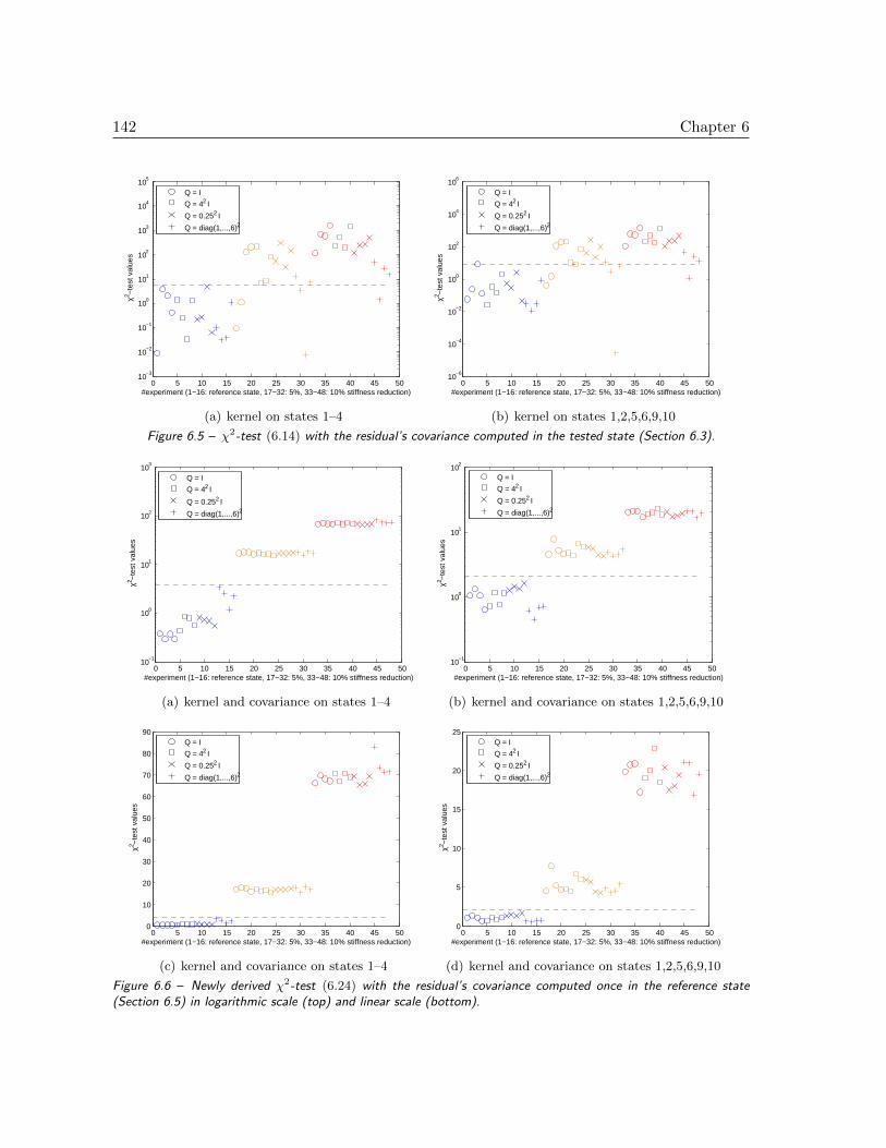
142 Chapter 6
0 5 10 15 20 25 30 35 40 45 5010
−3
10−2
10−1
100
101
102
103
104
105
#experiment (1−16: reference state, 17−32: 5%, 33−48: 10% stiffness reduction)
χ2 −te
st v
alue
s
Q = I
Q = 42 I
Q = 0.252 I
Q = diag(1,...,6)2
(a) kernel on states 1–4
0 5 10 15 20 25 30 35 40 45 5010
−6
10−4
10−2
100
102
104
106
#experiment (1−16: reference state, 17−32: 5%, 33−48: 10% stiffness reduction)
χ2 −te
st v
alue
s
Q = I
Q = 42 I
Q = 0.252 I
Q = diag(1,...,6)2
(b) kernel on states 1,2,5,6,9,10
Figure 6.5 – χ2-test (6.14) with the residual’s covariance computed in the tested state (Section 6.3).
0 5 10 15 20 25 30 35 40 45 5010
−1
100
101
102
103
#experiment (1−16: reference state, 17−32: 5%, 33−48: 10% stiffness reduction)
χ2 −te
st v
alue
s
Q = I
Q = 42 I
Q = 0.252 I
Q = diag(1,...,6)2
(a) kernel and covariance on states 1–4
0 5 10 15 20 25 30 35 40 45 5010
−1
100
101
102
#experiment (1−16: reference state, 17−32: 5%, 33−48: 10% stiffness reduction)
χ2 −te
st v
alue
s
Q = I
Q = 42 I
Q = 0.252 I
Q = diag(1,...,6)2
(b) kernel and covariance on states 1,2,5,6,9,10
0 5 10 15 20 25 30 35 40 45 500
10
20
30
40
50
60
70
80
90
#experiment (1−16: reference state, 17−32: 5%, 33−48: 10% stiffness reduction)
χ2 −te
st v
alue
s
Q = I
Q = 42 I
Q = 0.252 I
Q = diag(1,...,6)2
(c) kernel and covariance on states 1–4
0 5 10 15 20 25 30 35 40 45 500
5
10
15
20
25
#experiment (1−16: reference state, 17−32: 5%, 33−48: 10% stiffness reduction)
χ2 −te
st v
alue
s
Q = I
Q = 42 I
Q = 0.252 I
Q = diag(1,...,6)2
(d) kernel and covariance on states 1,2,5,6,9,10
Figure 6.6 – Newly derived χ2-test (6.24) with the residual’s covariance computed once in the reference state(Section 6.5) in logarithmic scale (top) and linear scale (bottom).

6.7 Conclusions 143
newly derived robust test γ2N = ξTN Σ−1ξ ξN in (6.24), where the residual’s covariance Σξ
is computed only once in the reference state (Section 6.5), in Figure 6.6.
For each state and excitation covariance, the 100 000 available samples were cut into 4 partswith sample length N = 25 000. The resulting χ2-test values of the three different tests onthis data are plotted in Figures 6.4, 6.5 and 6.6 in the following order: the first 16 test valuesare computed in the reference state, the next 16 values with 5% stiffness reduction and thelast 16 values with 10% stiffness reduction. In each of these states, 4 values correspond to oneof the 4 different excitation covariances mentioned above. An empirical threshold (horizontaldashed line) to distinguish between reference states and damaged states is computed on themean and variance of the χ2-test values of the 16 reference states.
As can be seen in Figure 6.4, the classical χ2-test is strongly influenced by a differentexcitation covariance and no separation of the χ2-test values between reference and damagedstates is possible. Recomputing the residual covariance on data of the currently tested statein Figure 6.5 already leads to a better separation between reference and damaged states,where less than 1/5 of the values in the damaged states are below the threshold establishedby the reference states. With the new robust χ2-test in Figure 6.6, a clear separation be-tween reference and damaged states is possible. Note also that the magnitude of damage isapparently linked to the obtained χ2-test values: Increasing the damage by factor 2 leads toχ2-test values that are approximately increased to factor 4, which is to be expected.
6.7 Conclusions
In this chapter, the influence of changing excitation between the reference state and thepossibly damaged state using the subspace-based fault detection test was clearly pointedout. Two modifications of the test are presented that take into account a changing ambientexcitation of the investigated system. The resulting fault detection tests thus contributeto the applicability of the tests under operation conditions, where the unmeasured ambientexcitation naturally varies. Especially the statistical fault detection test based on a noise-robust residual in Section 6.5 seems to be theoretically and practically promising. A study onreal data under varying excitation has to be made to validate the algorithms under operationconditions.
6.8 Dissemination
Parts of this chapter have been published in:
[LPS+09] M. Luczak, B. Peeters, W. Szkudlarek, L. Mevel, M. Dohler, W. Ostachowicz,K. Martyniuk, and K. Branner. Comparison of the three different approachesfor damage detection in the part of the composite wind turbine blade. In Proc.7th International Workshop on Structural Health Monitoring, Stanford, CA,USA, 2009.

144 Chapter 6
[DLM10b] M. Dohler, X.-B. Lam, and L. Mevel. Crystal clear data fusion in subspacesystem identification and damage detection. In Proc. 5th International Con-ference on Bridge Maintenance, Safety and Management, Philadelphia, PA,USA, 2010.
[DM10] M. Dohler and L. Mevel. Modular subspace-based system identification anddamage detection on large structures. In Proc. 34th International Symposiumon Bridge and Structural Engineering, Venice, Italy, 2010.
[DM11d] M. Dohler and L. Mevel. Robust subspace based fault detection. In Proc.18th IFAC World Congress, Milan, Italy, 2011.

Chapter 7
Robust subspace-based damagelocalization using mass-normalized
mode shapes
7.1 Introduction
Statistical subspace-based methods using output-only data have been shown to offer a robustsolution to the damage detection task where changes in the modal parameters of a structureare detected [MHVdA99, BAB00]. These techniques have also been combined with sensitivi-ties extracted from finite element models to localize damages: the detection of changes in localstructural parameters (e.g. stiffness) indicates the location of a damage [BMG04, BBM+08].Like this, the damage localization problem is formulated as detection problem.
In the formulation of this detection problem, all available structural parameters are testedseparately for a change using a χ2-test statistics. Comparing their values the damage can belocalized, when structural parameters are linked to a location, as high χ2 values indicate ahigh change. In the derivation of these tests in [BMG04, BBM+08], no special care was takenof the mutual influence of close structural parameters. The main drawback for localization isthen the possible reaction when testing an undamaged element due to the lack of orthogonalityin the parametric space defined by the corresponding χ2-metric. A robust version of this testis derived in this chapter. It yields more contrasted damage localization results between safeand damaged elements and thus reduces false alarms.
For damage localization, sensitivities of the modal parameters with respect to the moni-tored structural parameters are needed, that were computed from an a FEM of the investi-gated structure in [BMG04, BBM+08]. In some applications, though, the formulation of theFEM makes implementation impractical and this motivates the search for model-free damagelocalization alternatives. Without a FEM, sensitivities with respect to structural parameters
146 Chapter 7
can still be computed at the measured coordinates of a structure using mass-normalized modeshapes, which can be obtained by adding a known perturbation to the mass distribution ofthe structure and repeating the output-only identification [PVGVO02, BA03, Ber04, Ber11d].In this chapter, the corresponding model-free statistical damage localization test is derivedand illustrated on simulated data.
This chapter is organized as follows. In Section 7.2, the basic principles of subspace-basedsystem identification and statistical fault detection on vibrating structures are recalled fromChapter 2, as well as the damage localization test from [BMG04, BBM+08]. In Section 7.3,the problem of the mutual influence of structural parameters in the χ2-tests is addressed anda robust min-max test is considered. In Section 7.4, the FE model-free damage localizationtest is derived, using mass perturbations to obtain required sensitivities with respect tothe structural parameters in the reference state. The performance of the robust damagelocalization, where all required parameters are obtained without a model, are demonstratedin a simulation study in Section 7.5.
7.2 Statistical subspace-based damage localization
7.2.1 Models and parameters
The behaviour of a mechanical system is assumed to be described by a stationary lineardynamical system
M X (t) + C1X (t) +KX (t) = υ(t)
Y (t) = LX (t)(7.1)
where t denotes continuous time, M,C1,K ∈ Rm×m are the mass, damping and stiffnessmatrices, high-dimensional vector X collects the displacements of the m degrees of freedomof the structure, the non-measured external force ν modeled as non-stationary Gaussianwhite noise, the measurements are collected in the vector Y and matrix L indicates thesensor locations. The eigenstructure of (7.1) with the modes µ and mode shapes ϕµ is asolution of
det(µ2M + µC1 +K) = 0, (µ2M + µC1 +K)φµ = 0, ϕµ = Lφµ. (7.2)
Sampling model (7.1) at some rate 1/τ yields the discrete model in state-space form
Xk+1 = AXk + Vk
Yk = CXk
(7.3)
of model order n = 2m, whose eigenstructure is given by
det(A− λI) = 0, (A− λI)φλ = 0, ϕλ = Cφλ. (7.4)
Then, the eigenstructure of the continuous system (7.1) is related to the eigenstructure ofthe discrete system (7.3) by
eτµ = λ, ϕµ = ϕλ. (7.5)

7.2 Statistical subspace-based damage localization 147
The modal frequencies f and damping coefficients ρ are recovered directly from the eigenval-ues λ by
f =a
2πτ, ρ =
100|b|√a2 + b2
, (7.6)
where a = | arctan<(λ)/=(λ)| and b = ln |λ|.The collection of modes and mode shapes (λ, ϕλ) is a canonical parameterization of system
(7.3) and considered as the system parameter θ with
θ =
[Λ
vec Φ
], (7.7)
where Λ is the vector whose elements are the eigenvalues λ and Φ is the matrix whose columnsare the mode shapes ϕλ.
7.2.2 Stochastic Subspace Identification
To obtain the system parameter θ from output-only measurements (Yk)k=1,...,N , a SSI method
from Section 2.2.3 is used. From the data, a subspace matrix H is computed, which is anestimate of a theoretical subspace matrix H according to the selected method. It possessesthe factorization property
H = OZ (7.8)
into observability matrix
O =
C
CA...
CAp
and another matrix Z according to the selected method. An estimate O is obtained from Hby an SVD and truncation at the desired model order of
H =[U1 U0
] [∆1 0
0 ∆0
]V T , O = U1∆
1/21 .
From the observability matrix O an estimate of matrix C is obtained from its first blockrow. An estimate of A is obtained from a least squares solution using the shift invarianceproperty of O. Estimates of the eigenstructure (λ, ϕλ) of the system (7.3) and hence thesystem parameter θ are then obtained in (7.4).
7.2.3 Damage detection
In this section, the statistical subspace-based damage detection from Section 2.3 is recalled,where a residual function for damage detection is associated with the covariance-driven

148 Chapter 7
output-only subspace identification described in the previous section. This function com-pares the system parameter θ0 of a reference state with a subspace matrix H computed onnew data corresponding to an unknown, possibly damaged state.
Assume that the eigenvectors of A are chosen as the basis for the state space of system(7.3). Then, the observability matrix writes as
O(θ) =
Φ
Φ∆...
Φ∆p
with Φ and Λ as in (7.7) and ∆ = diag(Λ). Let S(θ0) be the left null space of O(θ0), whichcan be obtained by an SVD of O(θ0). Then, because of (7.8), the characteristic property ofthe system in the reference state writes
S(θ0)T H = 0.
For checking whether new data agree with the reference state corresponding to θ0, the residualfunction
ζN (θ0) =√N vec(S(θ0)
T H) (7.9)
is introduced in Section 2.3. Let J (θ0) and Σ(θ0) be the residual sensitivity and covariancematrices. The residual function is asymptotically Gaussian with
ζN (θ0)N−→
N (0,Σ(θ0)) no change
N (J (θ0) δθ,Σ(θ0)) change δθ(7.10)
Hence, a change in the system parameter θ corresponds to a change in the mean value ofthe residual function. It manifests itself in the χ2-test statistics
χ2N = ζN (θ0)
T Σ−1J (J T Σ−1J )−1J T Σ−1ζN (θ0),
where J and Σ are consistent estimates of J (θ0) and Σ(θ0) (cf. Section 2.3.3). To assess theoccurrence of damage, the value χ2
N should be compared with a threshold.
7.2.4 Damage localization
In [BMG04, BBM+08], the damage localization problem is stated as a detection problem asfollows: Let a set of structural parameters p1, . . . , pP be given, which are physically linkedto locations at the investigated structure. Assume that a change δpk occurs in one of theparameters pk. Then, the mean of the residual function ζN (θ0) in (7.10) can be expressed as
J (pk)δpk, k = 1, . . . , P,
where J (pk) is the sensitivity of the residual function with respect to pk and is usuallyobtained as
J (pk) = J (θ0)∂θ0∂pk
. (7.11)

7.3 Mutual influence of structural parameters in change detection test 149
Then, testing the parameters pk separately for a change consists in computing the residualζN (θ0) once in (7.9) and computing the χ2-test statistics
χ2N (pk) = ζN (θ0)
T Σ−1Jk(J Tk Σ−1Jk)−1J Tk Σ−1ζN (θ0) (7.12)
for each k = 1, . . . , P , where Jk is a consistent estimate of J (pk). Then, the values χ2N (pk),
k = 1, . . . , P , indicate the changes in the structural parameters pk. As the parameters arerelated to locations at the structure, high values of χ2
N (pk) indicate the location of the damage.The χ2-test statistics (7.12) is also called sensitivity test.
However, the sensitivity test assumes that a change happens in the tested structuralparameter and that every other parameter remains unchanged. This condition is violatedin two occasions, firstly when damage happen simultaneously at two or more locations, andmore important, when testing for a change in an unchanged structural element. In that case,the test will still react by statistical influence of the damage element. This effect will beconsidered in the next section.
7.3 Mutual influence of structural parameters in change de-tection test
7.3.1 Focused change detection in structural parameters
In the previous section, the sensitivity test (7.12) is computed to test a change in eachparameter pk, k = 1, . . . , P . Formally, δpk = 0 is tested against δpk 6= 0, by assuming nochange in the other parameters. This also means that χ2
N (pk) might be sensitive to a changein some other parameters pi with i 6= k [Bas97, BBMN09]. In the following, the min-maxapproach [Bas97] is described that consists in viewing the parameters pi, i 6= k, as nuisance.They are rejected by replacing them in the likelihood with their least favorable value. Then,for each parameter pk, the min-max approach detects a change in its corresponding directionof the parameter space, orthogonal to every direction corresponding to the set of the remainingparameters. Thus, changes in the remaining parameters do not affect the min-max test of theactually tested parameter. It also means that testing an undamaged element will not yield afalse alarm provoked by some other close damaged element. Note that for simplicity of thenotation, the symbol indicating a consistent estimate of the underlying variable, is omittedon the Jacobians J and the covariance matrix Σ.
Fix some k and define the Jacobians
Ja def= J (pk),
Jb def=[J (p1) · · · J (pk−1) J (pk+1) · · · J (pP )
]. (7.13)
The asymptotic Fisher information on the set of parameters p1, . . . , pP contained in ζN (θ0)is defined as
Fdef=[Ja Jb
]TΣ−1
[Ja Jb
]=
[Faa Fab
Fba Fbb
], (7.14)

150 Chapter 7
where
Faa = J Ta Σ−1Ja, Fab = J Ta Σ−1Jb,Fba = J Tb Σ−1Ja, Fbb = J Tb Σ−1Jb.
Furthermore, define the matrices
F ∗adef= Faa − FabF−1bb Fba,
the partial residuals
ζadef= J Ta Σ−1ζN (θ0), ζb
def= J Tb Σ−1ζN (θ0) (7.15)
and the robust residualζ∗a
def= ζa − FabF−1bb ζb. (7.16)
Then, the corresponding χ2-test statistics detecting a change in parameter pk writes as
χ∗2N = ζ∗Ta F ∗−1a ζ∗a (7.17)
and is not affected by a change in the parameters pi, i 6= k. Test (7.17) is called the min-maxtest. Hence, repeating the steps (7.13)–(7.17) for all k = 1, . . . , P leads to values of theχ2-test statistics (7.17) for each monitored structural parameter. A change in a parameter islinked with a high value of its corresponding χ2-test statistics and thus can be located.
Some comments are in order. First, it is obvious that the min-max test does not dependon the magnitude of the Jacobians, but only on the change directions defined by them. Thisis proven in the following lemma.
Lemma 7.1 The min-max test (7.17) is invariant to post-multiplication of the Jacobians Jaand Jb with some invertible matrices.
Proof: Use the notation from Equations (7.14)–(7.17) for the min-max test with theJacobians Ja and Jb. Now consider JaA and JbB instead of Ja and Jb for the min-maxtest, where A and B are some invertible matrices, and use the notation with a tilde ˜ for therespective variables in the min-max test. Then,
F =
[Faa Fab
Fba Fbb
]=
[ATJ Ta Σ−1JaA ATJ Ta Σ−1JbBBTJ Tb Σ−1JaA BTJ Tb Σ−1JbB
]=
[ATFaaA ATFabB
BTFbaA BTFbbB
]
and, furthermore,F ∗a = Faa − FabF−1bb Fba = ATF ∗aA.
Then, from (7.15) and (7.16) follows
ζ∗a = AT ζ∗a
and thus
χ∗2N = ζ∗Ta F ∗−1a ζ∗a =(AT ζ∗a
)T (ATF ∗aA
)−1 (AT ζ∗a
)= ζ∗Ta F ∗−1a ζ∗a = χ∗2N ,
7.3 Mutual influence of structural parameters in change detection test 151
proving the assertion.
There are many numerically sensitive operations involved in computing the min-maxtest in Equations (7.14)–(7.17). In [ZB03] the following practical and numerically stablecomputation was derived.
Lemma 7.2 ([ZB03]) Let Σ−1/2 be a square root inverse of Σ, such that
Σ−1 = (Σ−1/2)TΣ−1/2.
If Σ−1/2Ja and Σ−1/2Jb are full column rank, then the min-max test (7.17) writes as
χ∗2N = ξT ξ where ξ = QTc Σ−1/2ζN (θ0),
where Qc is obtained from the thin QR decompositions
Σ−1/2Ja = QaRa,
Σ−1/2Jb = QbRb,
Qa −QbQTb Qa = QcRc.
Note that for the computation of Σ−1/2 in the previous lemma from an estimate of Σ, thesame techniques as in Section 3.5.1 can be used.
7.3.2 Change directions and separability of structural parameters
With the described χ2-tests, structural parameters are tested for a change. This correspondsto testing directions in the structural parameter space for a change that are defined by thesensitivities of the structural parameters. These parameters might show some dependence,i.e. a change in one parameter might raise the χ2-test value of another parameter and viceversa. For checking the separability of these parameters, the angles between their respectivechange directions can be analyzed.
To be coherent with the χ2-metric, define the k-th change direction as [BMG04]
dkdef= Σ(θ0)
−1/2J (pk), k = 1, . . . , P, (7.18)
where Σ(θ0)−1/2 is a matrix square root of the inverse of Σ(θ0). The sensitivity test (7.12),
testing separately for changes in the parameters pk, k = 1, . . . , P , is hence a directional test,where the residual function ζN (θ0) is tested for a change in the directions dk in the structuralparameter space. Let the cosine of the angle between two change directions be given as
αijdef=
dTi dj‖di‖ ‖dj‖
, where ‖d‖ =√dTd. (7.19)
Thus, if αij ≈ 0 the change directions di and dj are nearly orthogonal and clearly separable.However, if |αij | ≈ 1, the change directions di and dj are nearly parallel and not separableanymore. In the latter case, changes in the parameters pi and pj are not distinguishable.Then, a change in parameter pi leads to similar values of the corresponding sensitivity testfor parameters pi and pj for |αij | ≈ 1.

152 Chapter 7
7.3.3 Clustering and rejection
Often, the number of structural parameters P is very high and especially higher than thenumber of modal parameters dim θ0 = 2m(r + 1). Then, many of the respective changedirections dk, k = 1, . . . , P , cf. (7.18), are nearly parallel with respect to the χ2-metric.Testing them separately in the sensitivity test then yields nearly the same results. Forthis problem, a clustering step was suggested in [BMG04, BBM+08] prior to testing allthe parameters, where each cluster contains nearly parallel change directions. Then, in thetest only a barycenter of each cluster is tested and the resulting χ2-value is assigned to allelements of the cluster. As the elements in one cluster are not (or very poorly) separable,all the elements of a cluster are either recognized as healthy or as damaged. Changing thesensor positions could lead to a separation of the cluster elements.
This clustering is even more important for the min-max test than the sensitivity testregarding the rejected parameters. It is not meaningful to test a parameter for a change inthe min-max test while rejecting another parameter whose change direction is nearly parallelto the tested parameter. This might lead to a low (false negative) result of the test, even ifa change in the parameter happened.
A clustering algorithm usually works in two steps. In the first step, small change direc-tions dk are removed, as vectors with a low magnitude are likely to blur the results of theaggregation. Then, the remaining vectors dk are normed to 1, as only their direction is ofinterest, and clustered. In [BMG04, BBM+08], a vector quantization method [LBG80, Gra84]is suggested for clustering, which performs a hierarchical classification while controlling thevariability in each cluster. However, any appropriate clustering algorithm can be used.
Let Nc the number of clusters and ck, k = 1, ..., Nc, be their barycenters. The barycentersare arbitrarily scaled, but because of Lemma 7.1 they can be directly used for the min-maxtest. With the definition of the change directions in (7.18) and with Lemma 7.2, the min-maxtest for each cluster k is performed as follows:
1. Define Ca = ck, Cb =[c1 . . . ck−1 ck+1 . . . cNc
];
2. Do thin QR decompositions
Ca = QaRa,
Cb = QbRb,
Qa −QbQTb Qa = QcRc;
3. Compute ξ = QTc Σ−1/2ζN (θ0) and finally χ∗2N (ck) = ξT ξ. Assign value χ∗2N (ck) to allelements in cluster k.
In Section 9.3, the damage localization using the min-max approach with clustering isperformed on a simulated bridge deck with almost 10 000 elements.

7.4 Damage localization using mass-normalized mode shapes from mass perturbations 153
7.4 Damage localization using mass-normalized mode shapesfrom mass perturbations
For the statistical damage localization approach in [BMG04, BBM+08], the monitored struc-tural parameters pk are stiffness parameters of a FEM. The sensitivities ∂θ0/∂pk in (7.11)of the modal parameters with respect to the structural parameters are obtained from thesettings of a FEM. They are needed for the sensitivity test (7.12) or the min-max test (7.17).
In this section, this approach is modified to work without a FEM. The considered struc-tural parameters pk are masses and stiffnesses with respect to the measured coordinates ofthe structure. The required sensitivities for these structural parameters can be computed us-ing mass-normalized mode shapes, which can be obtained from Operational Modal Analysisby two measurements of a structure, where a known mass perturbation is introduced on thestructure between the measurements.
7.4.1 Mass-normalization of mode shapes using mass perturbations
Output-only system identification cannot provide mode shapes that are mass-normalized,such that the collection of eigenvectors φ from (7.2) yields
ΩTMΩ = I, (7.20)
where the columns of Ω are the eigenvectors φ. In order to solve this problem, Parloo et al.[PVGVO02] proposed a method using system identification results from two measurementsof the structure where a known mass perturbation ∆M is introduced at (some or all of)the measured coordinates between the two measurements. Since, further mass-normalizationmethods using mass perturbations have been developed, see e.g. [BA03, Ber04, Ber11d], anda review in [Ber11a]. It turns out that the mode shapes ϕ, which are obtained only at themeasured degrees of freedom, can be normalized without knowing the unobserved part. Inthe following, we use the receptance based approach from [Ber11d] using the normal modemodel, where the modal parameters are obtained from
det(K − ω2M) = 0, Kφ = ω2Mφ, ϕ = Lφ,
cf. (7.2). For the natural frequencies f holds ω = 2πf .Denote a mode and corresponding mode shape of the structure in the original state by ωi
and ϕi and after the mass perturbation ∆M on the structure by ω∗i and ϕ∗i , for i = 1, · · · ,m.The modal scaling factors βi are defined such that
ψi = βiϕi (7.21)
are the mass-normalized mode shapes fulfilling (7.20). With the receptance based approach
from [Ber11d], the squares of the modal scaling factors γidef= β2i are obtained from the linear
set of equations described by
m∑
l=1
ϕl(ϕTl ∆Mϕ∗j )ω
2∗j
ω2l − ω2∗
j
γl = ϕ∗j , j = 1, . . . ,m, (7.22)
154 Chapter 7
by a least squares solution. Then, with the mass-normalized mode shapes (7.21), sensitivitieswith respect to some structural parameters can be computed.
Remark 7.3 In this section, the normal mode model was used without considering damping,while in (7.2) the complex mode model was used. While the latter model is probably moreappropriate for vibrating structures under operation conditions, the imaginary parts of themode shapes and the estimated damping values are possibly not very reliable for the sen-sitivity computation in the following. These figures were already skipped in the sensitivitycomputations using FEM data in [BBM+08]. This is also the reason why the complex modemass normalization as e.g. in [Ber11c] is not used here.
7.4.2 Sensitivities of modal parameters with respect to structural param-eters
Using the mass-normalized mode shapes ψi, i = 1, . . . ,m, the sensitivities of the modal pa-rameters with respect to a mass ms at the measured coordinate s or with respect to a stiffnesskst, which is assumed between the measured coordinates s and t, can be computed as de-scribed in [HLS98]. Let ψji be the j-th entry of mode shape ψi. Then, the desired sensitivitiesare
∂ωims
= −1
2ωiψ
2si
∂ψjims
= −1
2ψ2siψji + ψsi
m∑
l=1,l 6=i
ω2i
ω2l − ω2
i
ψslψjl
(7.23)
for the sensitivities with respect to mass and
∂ωikst
= − 1
2ωi(ψsi − ψti)2
∂ψjikst
= (ψsi − ψti)m∑
l=1,l 6=i
1
ω2l − ω2
i
(ψsl − ψtl)ψjl(7.24)
for the sensitivities with respect to stiffness.
7.4.3 Sensitivities for χ2-tests
For localization of changes in the mass at the measured coordinates of the structure and local-ization of changes in the stiffness of assumed structural elements between pairs of measuredcoordinates of the structure, the considered structural parameters are pk = ms or pk = kst.In (7.23) and (7.24) sensitivities of modal parameters with respect to these structural pa-rameters are given. It remains the computation of J (pk) = J (θ0)∂θ0/∂pk in (7.11) for thesensitivity test (7.12) or min-max test (7.17).
In Section 2.3.3 the residual sensitivity J (θ0) with respect to the modal parameter isderived. The modal parameter θ0 contains the modes λ of the discrete system (7.4). However,in the previous section sensitivities of the pulsations ω of the continuous system (7.1) are givenw.r.t. structural parameters. To compute the sensitivity J (pk) of the residual ζN (θ0) with

7.5 Numerical results 155
respect to the structural parameters, the sensitivity Jλω of the eigenvalues λ with respect tothe pulsations ω = 2πf is needed, which results directly from relation (7.6) and is detailed in[BMG04]. Then, the desired sensitivities of the residual w.r.t. structural parameters write as
J (pk) = J (θ0)JλωJpk , (7.25)
where Jpk is the collection of sensitivities of (7.23) or (7.24) in a column vector, dependingon the kind of structural parameter. Note that in this derivation the system parameter θ0 (onwhich J (θ0) is computed) must contain the mass-normalized mode shapes to be coherent.
7.4.4 Summary of model-free damage localization algorithm
Damage localization usually corresponds to finding the element(s) of a structure with thehighest change of stiffness compared to a reference state. With the derivations in the previoussections we can detect changes in mass (pk = ms) or in stiffness (pk = kst) with a statisticaltest. The resulting algorithm for model free damage localization consists of the followingsteps:
1. Output-only measurement of the structure in the reference state, retrieval of modalparameter θ0,1 from Stochastic Subspace Identification (SSI) (Section 7.2.2),
2. Add a mass perturbation ∆M near one or more sensor positions, do output-only mea-surements and retrieve modal parameter θ0,2 from SSI,
3. Compute mass-normalized mode shapes using θ0,1 and θ0,2 (Equations (7.21), (7.22))and replace arbitrarily scaled mode shapes from θ0,1 by mass-normalized mode shapesto obtain system parameter θ0,
4. Computation of J (pk), k = 1, . . . , P , (Equations (7.23)–(7.25)) and Σ(θ0) in the refer-ence state,
5. Computation of χ∗2N (pk), k = 1, . . . , P , in possibly damaged states (Equations (7.13)–(7.17)) and comparison of their values. A high value χ∗2N (pk) is linked to a high changein pk.
7.5 Numerical results
To validate the proposed min-max test for a focused change detection in the structural pa-rameters and the statistical-based model-free damage localization algorithm, a simulationstudy was made using a mass-spring model of six degrees of freedom (Figure 7.1). Using thismodel, output-only data was generated at all 6 DOFs to obtain the necessary measurementsin the reference states for the mass-normalization of the mode shapes and in the damagedstates with different introduced damage scenarios.
In the reference state, the modal parameter θ0,1 was obtained from SSI. After an increaseof the mass at DOF 2 of 5%, the modal parameter θ0,2 was obtained from SSI. Both wereused to compute the mass-normalized mode shapes, which are also inserted in the reference
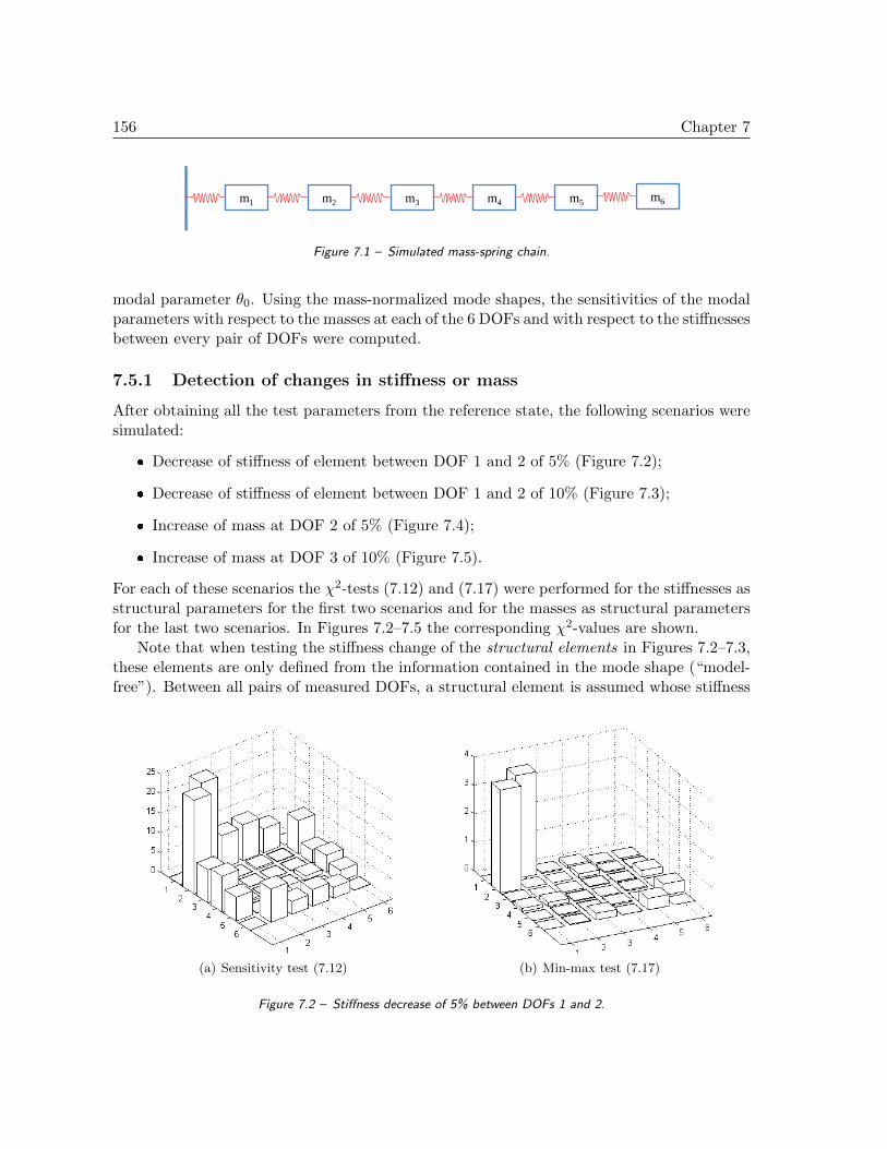
156 Chapter 7
m1 m2 m3 m4 m5m6
Figure 7.1 – Simulated mass-spring chain.
modal parameter θ0. Using the mass-normalized mode shapes, the sensitivities of the modalparameters with respect to the masses at each of the 6 DOFs and with respect to the stiffnessesbetween every pair of DOFs were computed.
7.5.1 Detection of changes in stiffness or mass
After obtaining all the test parameters from the reference state, the following scenarios weresimulated:
Decrease of stiffness of element between DOF 1 and 2 of 5% (Figure 7.2);
Decrease of stiffness of element between DOF 1 and 2 of 10% (Figure 7.3);
Increase of mass at DOF 2 of 5% (Figure 7.4);
Increase of mass at DOF 3 of 10% (Figure 7.5).
For each of these scenarios the χ2-tests (7.12) and (7.17) were performed for the stiffnesses asstructural parameters for the first two scenarios and for the masses as structural parametersfor the last two scenarios. In Figures 7.2–7.5 the corresponding χ2-values are shown.
Note that when testing the stiffness change of the structural elements in Figures 7.2–7.3,these elements are only defined from the information contained in the mode shape (“model-free”). Between all pairs of measured DOFs, a structural element is assumed whose stiffness
(a) Sensitivity test (7.12) (b) Min-max test (7.17)
Figure 7.2 – Stiffness decrease of 5% between DOFs 1 and 2.

7.5 Numerical results 157
(a) Sensitivity test (7.12) (b) Min-max test (7.17)
Figure 7.3 – Stiffness decrease of 10% between DOFs 1 and 2.
(a) Sensitivity test (7.12) (b) Min-max test (7.17)
Figure 7.4 – Mass of 5% added at DOF 2.
(a) Sensitivity test (7.12) (b) Min-max test (7.17)
Figure 7.5 – Mass of 5% added at DOF 3.

158 Chapter 7
change is tested. Hence, also elements are tested that do not exist in the underlying simulatedmodel (e.g. elements (1,3), (1,4), . . . ), as no information of this model is used. For testingthe mass change in Figures 7.4–7.5, the mass at each measured DOF is tested.
In each case, the location of the change of the structural parameter could be clearlyidentified. The min-max test (7.17) using the rejection approach gives higher contrasted testresults and thus outperforms the sensitivity test (7.12).
7.5.2 Detection of changes in stiffness while rejecting changes in mass
In another simulated scenario, both the mass and stiffness of the model were changed witha 5% increase of mass at DOF 2 and 5% stiffness reduction between DOFs 1 and 2. For
(a) Sensitivity test (7.12)
(b) Min-max test (7.17) rejecting other stiffness pa-rameters
(c) Min-max test (7.17) rejecting other stiffness andmass parameters
Figure 7.6 – Mass of 5% added at DOF 2 and stiffness decrease of 5% between DOFs 1 and 2.

7.5 Numerical results 159
example, such a situation can happen in practice when monitoring a bridge for damage,where the traffic is regarded as a nuisance. Not the added weight to the bridge should bedetected, but the damage in the bridge, i.e. the stiffness change of the bridge’s structuralelements. Similarly, the changes due to the mass of water in an aqueduct or at a dam shouldbe rejected, while monitoring the structural integrity. Of course, the presented example onthe 6 DOF mass-spring chain only reflects this idea, but not an entire structure.
In Figure 7.6(a), the sensitivity test is shown, where many elements besides the damagedelement (1,2) clearly react. In a first step, the non-tested stiffness parameters were rejectedwith the min-max test in Figure 7.6(b), similar to the previous section. In the last step, alsothe mass parameters were rejected in Figure 7.6(c), leading to the highest contrasted resultof the test and underlining the importance of the rejection approach. Note also, that only inFigure 7.6(c), the χ2-value of the damaged element of around χ2 ≈ 3 corresponds to Figure7.2(b), where the stiffness of element (1,2) was also decreased by 5%. Thus, the rejectionapproach seems to be indispensable for a quantification of the damages.
7.5.3 Orthogonality of change directions
Although only one parameter was changed in each of the experiments in Figures 7.2–7.5, theχ2-test statistics also reacted for some of the structural quantities that were not changed. Forthe sensitivity tests (7.12) in the figures, the reason for this reaction is obvious: Computingthis test on unaffected structural parameters (mass or stiffness) is performed while still beingsensitive to changes in other parameters (amongst them one modified parameter) and thusmight lead to a false alarm.
Now consider the min-max test (7.17) in Figures 7.2(b)–7.5(b). The χ2 value correspond-ing to an unmodified structural parameter reacts less. Still, for some elements the min-maxtest reacts, e.g. for testing a change in the stiffness of the elements (1,3), (2,4), (3,6), (4,5) or(5,6), even if only the stiffness of element (1,2) was reduced (see Figures 7.2(b) and 7.3(b)).Similarly, when testing for a mass change at DOF 5, the test reacts, when the mass at DOF 2was increased in Figure 7.4(b). Also, the test at DOF 4 reacts, when the mass at DOF 3 wasincreased in Figure 7.5(b). This can be explained by looking at the angles between the un-derlying change directions that are tested: In all these cases, the cosine of the angle between
Table 7.1 – Cosine of angles between change direction corresponding to change of stiffness of element (1,2) andthe elements (a,b)
a \ b 1 2 3 4 5 6
1 – 1.00 0.83 0.16 0.87 0.30
2 1.00 – 0.22 0.82 0.27 0.28
3 0.83 0.22 – 0.18 0.11 0.86
4 0.16 0.82 0.18 – 0.87 0.80
5 0.87 0.27 0.11 0.87 – 0.86
6 0.30 0.28 0.86 0.80 0.86 –

160 Chapter 7
Table 7.2 – Cosine of angles between change direction corresponding to change of mass of DOF a and DOF b
a \ b 1 2 3 4 5 6
1 1.00 0.34 0.22 0.30 0.36 0.87
2 0.34 1.00 0.77 0.79 0.91 0.30
3 0.22 0.77 1.00 0.90 0.74 0.14
4 0.30 0.79 0.90 1.00 0.79 0.22
5 0.36 0.91 0.74 0.79 1.00 0.32
6 0.87 0.30 0.14 0.22 0.32 1.00
the corresponding change directions computed from (7.19) was quite high (see Tables 7.1and 7.2), thus indicating a poor separability of the underlying structural parameters. Never-theless, the test of the changed parameter still reacts stronger than the test of (unchanged)parameter having a nearly parallel change direction.
7.6 Conclusions
In this chapter, a model-free subspace-based statistical damage localization test was derivedfor output-only data using known mass perturbations of the structure in the reference state.Its performance to detect changes in the stiffness or mass between the measured coordinates ofa structure was demonstrated using simulated data. When testing the structural parametersfor a change, special care was taken of the rejection of the influence of the other structuralparameters that are not actually tested. The effectiveness of this rejection was demonstratedas well and it seems to be important for future damage quantification. An application of thedamage localization to a simulated bridge deck using the clustering and rejection approach isdemonstrated in Section 9.3. Future work contains the validation of the proposed algorithmson a real structure.
7.7 Dissemination
Parts of this chapter have been published in:
[DBMS11] M. Dohler, D. Bernal, L. Mevel, and D. Siegert. Statistical-based model-freedamage localization. In Proc. 4th International Operational Modal AnalysisConference, Istanbul, Turkey, 2011.
[DMB11] M. Dohler, L. Mevel, and D. Bernal. Statistical subspace-based model-freedamage localization. In Proc. Engineering Mechanics Institute Conference,Boston, USA, 2011.

Part IV
Applications
161


Chapter 8
Modal analysis with multi-setupsystem identification
8.1 Introduction
In this chapter, the merging algorithms for multi-setup system identification from Chapter 4are applied to the eigenstructure identification of a composite plate and four civil structuresusing output-only vibration data. The data of all structures was recorded under operationalconditions, except for the composite plate, which was recorded in the lab. The analyses ofthe structures were made in the framework of numerous collaborations, which are gratefullyacknowledged.
The underlying mechanical model for vibration analysis and the transformation to a state-space model was presented in Section 2.4. Using the merging methods from Chapter 4 formulti-setup subspace system identification, the system matrices are identified at multiplemodel orders, where the fast multi-order algorithms from Chapter 5 are used. From theireigenstructure, the natural frequencies f , damping ratios ρ and mode shapes ϕ of the in-vestigated structure are determined. With the help of a stabilization diagram (see Section2.4.3), where the natural frequencies are plotted against model order, the true system modesare distinguished from spurious modes and the final model is obtained. This final model ischosen manually from the stabilization diagram. One example of multi-setup and multi-ordersystem identification is Z24 Bridge, which were detailed in Sections 4.7 and 5.5.
For the application of the merging algorithms, one of the Algorithms 4.1–4.5 is used eitherwith covariance-driven SSI or the data-driven UPC algorithm. As the merging algorithmsmainly differ in their implementation and no SSI algorithm with left weighting is used, anyone of them can be used, yielding practically identical identification results. In the imple-mentation of the merging algorithm the results of Section 4.5 are used, as the true modelorder is unknown.

164 Chapter 8
Often, a comparison for multi-setup system identification with further, empirical mergingmethods is made by the collaborating partners. Their notation and schematic is introducedin Section 8.2, before the modal analysis of the mentioned structures is made in Section 8.3.In Section 8.4, the results of the multi-setup identification are discussed and the relevance ofthe new merging algorithms from Chapter 4 is pointed out.
8.2 Notation and comparison to other methods
For eigenstructure identification from multiple sensor setups, mainly three strategies are inuse [Par03, Sec. 3.3], [RMDRC09] that consist of the general steps
normalization (scaling) due to different ambient excitation or identification results,
merging of the data or identification results,
eigenstructure identification.
According to the order of these steps, they are called Pre Global Estimation Re-Scaling(PreGER), Post Separate Estimation Re-Scaling (PoSER) and Post Global Estimation Re-Scaling (PoGER) in [Par03, RMDRC09]. For the application with SSI algorithms we will usethese notations.
The Pre Global Estimation Re-Scaling (PreGER) consists in the steps normalization –merging – identification. It comprises the algorithms from Chapter 4 and its schematics areillustrated in Figure 8.1.
H(1)
H(2)
H(Ns)
O(1,ref), O(1)
O(2)
O(Ns)
......
SVD + re-scaling
SVD + re-scaling
SVD + re-scaling
identificationmergingO(all) f , ρ, ϕ(all)
Figure 8.1 – Scheme of PreGER approach (Algorithm 4.4).
The Post Separate Estimation Re-Scaling (PoSER) [MK00, VdALMH00, CGDV02,Par03, RMDRC09, Au11] consists in the steps identification – normalization – merging. Itis the common practice approach for multi-setup system identification in Operational ModalAnalysis. The data of each setup is processed separately, yielding a set of model parameters(fj , ρj , ϕ
(j)) for each setup j. Then, the identified modes are matched between all setups andfinal estimates of frequencies and damping ratios are obtained by averaging. Before merging

8.2 Notation and comparison to other methods 165
H(1)
H(2)
...
H(Ns)
identification
identification
identification
f1, ρ1, ϕ(1)
f2, ρ2, ϕ(2)
fNs, ρNs
, ϕ(Ns)
...
f , ρ, ϕ(all)
re-scaling + merging
re-scaling + merging
re-scaling + merging
Figure 8.2 – Scheme of PoSER approach.
the partial mode shapes from each setup, they are re-scaled in a least-squares sense, for in-stance to the reference sensor part of the first setup. The whole procedure is summarized inFigure 8.2. For a large number of setups, this approach is time consuming as many stabiliza-tion diagrams have to be analyzed. Moreover, not all modes may be well excited in all setups,and often mode pairing between different setups is difficult due to closely spaced modes.
The Post Global Estimation Re-Scaling (PoGER) [Par03, PGC03, RMDRC09] consists inthe steps merging – identification – normalization. For SSI algorithms, this empirical mergingapproach consists in the computation of the subspace matrix for each setup separately andmerging them directly to a global subspace matrix. Then, system identification is performed,yielding one set of global modal parameters. Due to a possibly different excitation in eachsetup, the mode shape estimates are finally rescaled in a least squares sense with respect totheir reference sensor part. The procedure is summarized in Figure 8.3.
replacements
H(j) | j = 1, . . . , Nsidentification
f , ρ
ϕ(1)
ϕ(Ns)
...f , ρ, ϕ(all)
re-scaling
Figure 8.3 – Scheme of PoGER approach.
For a comparison of mode shapes obtained from different methods and for evaluating theorthogonality between a set of mode shapes, the Modal Assurance Criterion (MAC) is used,which is the angle between two mode shapes and defined as
MAC(ϕ1, ϕ2)def=
|ϕ∗1ϕ2|√ϕ∗1ϕ1
√ϕ∗2ϕ2
.

166 Chapter 8
A MAC value near to 1 indicates thus a strong similarity between two mode shapes, and avalue near to 0 rather orthogonal mode shapes.
8.3 Case studies
8.3.1 A composite plate
Within a collaboration with LMS (Belgium), the Risø laboratory (Denmark) and the PolishAcademy of Sciences, glass reinforced composite panels of dimension 20×320×320 mm wereinvestigated. They are similar to the load carrying laminate in a wind turbine blade [LS10]and are illustrated in Figure 8.4. They were also used for excitation robust damage detectionin Section 6.6.1.
Vibration measurements of the composite panels were made in the lab at a sampling rate
Figure 8.4 – Glass reinforced composite panel [LS10].
Figure 8.5 – Stabilization diagram containing the natural frequencies composite plate from covariance-driven SSIwith Algorithm 4.4.

8.3 Case studies 167
of 1/τ = 4096 Hz in Ns = 4 setups, where 3 of them contained 14 moving sensors and 1contained 7 moving sensors, with r(ref) = 1 reference sensor that stayed fixed all the time.Thus, the structure was recorded at altogether 49 measurement points.
With merging Algorithm 4.4 using covariance-driven SSI, a stabilization diagram wasobtained in Figure 8.5, from which the system modes were selected. Nine modes in the range[0− 2048 Hz] were obtained. Their mode shapes with their natural frequencies and dampingratios are displayed in Figure 8.6.
mode 1 - 359 Hz - 1.7% mode 2 - 554 Hz - 3.5% mode 3 - 784 Hz - 3.3%
mode 4 - 929 Hz - 2.7% mode 5 - 1097 Hz - 1.9% mode 6 - 1270 Hz - 5.0%
mode 7 - 1506 Hz - 2.4% mode 8 - 1850 Hz - 2.1% mode 9 - 1946 Hz - 1.7%
Figure 8.6 – Obtained natural frequencies, damping ratios and mode shapes of composite plate.
8.3.2 Luiz I Bridge
The multi-setup system identification of Luiz I Bridge was investigated within a collaborationwith KU Leuven (Belgium) and the Faculty of Engineering of University of Porto (Portu-gal). A prior study comparing different merging approaches on Luiz I Bridge was made in[RMDRC09], which is extended to the merging approach from Chapter 4.
8.3.2.1 Bridge description and ambient vibration test
The Luiz I Bridge (Figure 8.7) is a 172 m tied metallic arch bridge over the Douro River atthe city of Porto, in the north of Portugal, built in 1885 by Eiffel’s former engineer Theophile

168 Chapter 8
Seyrig. The bridge is composed by a hinged metallic arch supporting two different decks:one at the top of the arch and another one at the level of the respective supports. The archspans 172 m between abutments and rises 45.1 m. It has a variable thickness, between 16.7 mnear the supports and 7.1 m at midspan, and presents a parabolic geometry both in verticaland plan views. The upper deck is 391.25 m long and 5 m height, and it is supported by thearch, at midspan and at two intermediate sections, by 5 piers and the abutments. The lowerdeck has a height of 3.25 m, is suspended from the arch by four ties and provides a roadwayconnection between the cities of Porto and Vila Nova de Gaia.
The Laboratory of Vibrations and Monitoring (VIBEST) of the Civil Engineering De-partment of the Faculty of Engineering of the University of Porto (FEUP) was contracted toperform the ambient vibration tests on the Luiz I Bridge. This dynamic test was conductedwithout disturbing the normal use of the bridge, so the measured accelerations were mainlyinduced by the wind, by the roadway traffic on the lower deck and by the metro passing overthe upper deck. The dynamic response of the bridge was recorded with four seismographsequipped with triaxial force-balance accelerometers and duly synchronized by GPS. Becauseof the limited number of available sensors and the need to measure a high number of points,the measurements were carried out in 26 different setups during two days. For the vibrationrecordings, two recorders served as references, permanently located at section 15 (Figure 8.7),at both the upstream and downstream sides, while the other two recorders scanned the bridgedeck in 18 consecutive setups, measuring the acceleration along the 3 orthogonal directions,at both the upstream and downstream sides. During the ambient vibration test of the lowerdeck, the reference sensors of the upper deck kept their positions and an additional referencewas introduced at the downstream side at section 22 (Figure 8.7). For each setup, time seriesof 16 minutes were collected with a sampling frequency of 100 Hz. Further details of the
Figure 8.7 – Luiz I Bridge.

8.3 Case studies 169
dynamic test can be found in [CMC06].
The data to be processed consists of the lateral and vertical accelerations of the bridge,is low-pass filtered at 4 Hz and re-sampled with the sampling frequency 20 Hz.
8.3.2.2 Multi-setup system identification
In [RMDRC09], system identification results were obtained using the PoSER and PoGERapproaches with covariance-driven SSI. Altogether, 14 modes were identified. These resultsare not repeated here, but used for a comparison in the following section.
For the analysis with the PreGER approach (Algorithm 4.2) we separated the data intotheir lateral and vertical components and processed them separately. This led to better resultsthan processing the data from both directions together as the mode shape of a lateral bendingmode would contain noise in the vertical direction, and vice versa. Apart from this separation,all setups were processed together. For the analysis the parameters p + 1 = q = 150 werechosen and the model order ranged from 1 to 150. The modes were manually chosen in astable model order band in the resulting stabilization diagrams.
4.4 PreGER approach
For the analysis with the PreGER method we separated the data into their lateral and vertical components and
processed them separately because there are only purely lateral and purely vertical bending modes present in the
frequency range of interest. This led to better results than processing the data from both directions together as the
mode shape of a lateral bending mode would contain noise in the vertical direction, and vice versa. Apart from
this separation, all setups were processed together. For the analysis the half number of correlation lags was 150
(p = q = 150 in Equation (3)) and the model order ranged from 1 to 150. The modes were manually chosen in a
stable model order band in the resulting stabilization diagrams.
For the lateral components, one reference sensor common to all setups was available on the upper deck, and
for the vertical components, two reference sensors were available on the upper deck. With these settings all modes
from the PoSER approach could be identified, except mode 1 and 7 like in the PoGER approach. These are local
lateral bending modes of the lower deck, and the lateral reference sensor only from the upper deck was used.
Besides, an additional lateral bending mode was identified at 3.088Hz (mode 11A).In order to identify the local lateral bending modes of the lower deck, we continued the analysis only with the
setups containing data from the lower deck, including the reference sensor from the lower deck. This led to the
identification of modes 1 and 7, and an additional local lateral bending mode at 3.963Hz (mode 15). Another separateanalysis of the upper deck (with the reference sensor from there) led to the identification of a local lateral bending
mode of the upper deck at 3.393Hz (mode 13A). None of the modes 1, 7, 13A and 15 were present on both decks.
The stabilization diagrams with these different settings used for the modal extraction with the PreGER approach
can be found in Figure 8.
modelorder
frequency
50
100
150
0.0 0.5 1.0 1.5 2.0 2.5 3.0 3.5 4.0
(a) Vertical data, both decks (modes 5, 10, 11, 12, 13, 14)
modelorder
frequency
50
100
150
0.0 0.5 1.0 1.5 2.0 2.5 3.0 3.5 4.0
(b) Lateral data, both decks (modes 2, 3, 4, 6, 8, 9, 11A)
modelorder
frequency
50
100
150
0.5 1.0 1.5 2.0 2.5 3.0 3.5 4.0
(c) Lateral data, lower deck (modes 1, 7, 15)
modelorder
frequency
50
100
150
0.0 0.5 1.0 1.5 2.0 2.5 3.0 3.5 4.0
(d) Lateral data, upper deck (mode 13A)
Figure 8: Stabilization diagrams used to identify the modes in the PreGER approach.
All the identified mode shapes can be seen in Figure 9 and they correspond very well to the results of the PoSER
and the PoGER approach, as well as the frequencies and damping ratios. Only the damping ratio of mode 5 was
badly estimated as it has not stabilized yet in the stabilization diagram. Furthermore, the double mode 9 and 10
(a) Vertical data, both decks (modes 5, 10, 11, 12, 13,14)
4.4 PreGER approach
For the analysis with the PreGER method we separated the data into their lateral and vertical components and
processed them separately because there are only purely lateral and purely vertical bending modes present in the
frequency range of interest. This led to better results than processing the data from both directions together as the
mode shape of a lateral bending mode would contain noise in the vertical direction, and vice versa. Apart from
this separation, all setups were processed together. For the analysis the half number of correlation lags was 150
(p = q = 150 in Equation (3)) and the model order ranged from 1 to 150. The modes were manually chosen in a
stable model order band in the resulting stabilization diagrams.
For the lateral components, one reference sensor common to all setups was available on the upper deck, and
for the vertical components, two reference sensors were available on the upper deck. With these settings all modes
from the PoSER approach could be identified, except mode 1 and 7 like in the PoGER approach. These are local
lateral bending modes of the lower deck, and the lateral reference sensor only from the upper deck was used.
Besides, an additional lateral bending mode was identified at 3.088Hz (mode 11A).In order to identify the local lateral bending modes of the lower deck, we continued the analysis only with the
setups containing data from the lower deck, including the reference sensor from the lower deck. This led to the
identification of modes 1 and 7, and an additional local lateral bending mode at 3.963Hz (mode 15). Another separateanalysis of the upper deck (with the reference sensor from there) led to the identification of a local lateral bending
mode of the upper deck at 3.393Hz (mode 13A). None of the modes 1, 7, 13A and 15 were present on both decks.
The stabilization diagrams with these different settings used for the modal extraction with the PreGER approach
can be found in Figure 8.
modelorder
frequency
50
100
150
0.0 0.5 1.0 1.5 2.0 2.5 3.0 3.5 4.0
(a) Vertical data, both decks (modes 5, 10, 11, 12, 13, 14)
modelorder
frequency
50
100
150
0.0 0.5 1.0 1.5 2.0 2.5 3.0 3.5 4.0
(b) Lateral data, both decks (modes 2, 3, 4, 6, 8, 9, 11A)
modelorder
frequency
50
100
150
0.5 1.0 1.5 2.0 2.5 3.0 3.5 4.0
(c) Lateral data, lower deck (modes 1, 7, 15)
modelorder
frequency
50
100
150
0.0 0.5 1.0 1.5 2.0 2.5 3.0 3.5 4.0
(d) Lateral data, upper deck (mode 13A)
Figure 8: Stabilization diagrams used to identify the modes in the PreGER approach.
All the identified mode shapes can be seen in Figure 9 and they correspond very well to the results of the PoSER
and the PoGER approach, as well as the frequencies and damping ratios. Only the damping ratio of mode 5 was
badly estimated as it has not stabilized yet in the stabilization diagram. Furthermore, the double mode 9 and 10
(b) Lateral data, both decks (modes 2, 3, 4, 6, 8, 9,11A)
4.4 PreGER approach
For the analysis with the PreGER method we separated the data into their lateral and vertical components and
processed them separately because there are only purely lateral and purely vertical bending modes present in the
frequency range of interest. This led to better results than processing the data from both directions together as the
mode shape of a lateral bending mode would contain noise in the vertical direction, and vice versa. Apart from
this separation, all setups were processed together. For the analysis the half number of correlation lags was 150
(p = q = 150 in Equation (3)) and the model order ranged from 1 to 150. The modes were manually chosen in a
stable model order band in the resulting stabilization diagrams.
For the lateral components, one reference sensor common to all setups was available on the upper deck, and
for the vertical components, two reference sensors were available on the upper deck. With these settings all modes
from the PoSER approach could be identified, except mode 1 and 7 like in the PoGER approach. These are local
lateral bending modes of the lower deck, and the lateral reference sensor only from the upper deck was used.
Besides, an additional lateral bending mode was identified at 3.088Hz (mode 11A).In order to identify the local lateral bending modes of the lower deck, we continued the analysis only with the
setups containing data from the lower deck, including the reference sensor from the lower deck. This led to the
identification of modes 1 and 7, and an additional local lateral bending mode at 3.963Hz (mode 15). Another separateanalysis of the upper deck (with the reference sensor from there) led to the identification of a local lateral bending
mode of the upper deck at 3.393Hz (mode 13A). None of the modes 1, 7, 13A and 15 were present on both decks.
The stabilization diagrams with these different settings used for the modal extraction with the PreGER approach
can be found in Figure 8.
modelorder
frequency
50
100
150
0.0 0.5 1.0 1.5 2.0 2.5 3.0 3.5 4.0
(a) Vertical data, both decks (modes 5, 10, 11, 12, 13, 14)
modelorder
frequency
50
100
150
0.0 0.5 1.0 1.5 2.0 2.5 3.0 3.5 4.0
(b) Lateral data, both decks (modes 2, 3, 4, 6, 8, 9, 11A)
modelorder
frequency
50
100
150
0.5 1.0 1.5 2.0 2.5 3.0 3.5 4.0
(c) Lateral data, lower deck (modes 1, 7, 15)
modelorder
frequency
50
100
150
0.0 0.5 1.0 1.5 2.0 2.5 3.0 3.5 4.0
(d) Lateral data, upper deck (mode 13A)
Figure 8: Stabilization diagrams used to identify the modes in the PreGER approach.
All the identified mode shapes can be seen in Figure 9 and they correspond very well to the results of the PoSER
and the PoGER approach, as well as the frequencies and damping ratios. Only the damping ratio of mode 5 was
badly estimated as it has not stabilized yet in the stabilization diagram. Furthermore, the double mode 9 and 10
(c) Lateral data, lower deck (modes 1, 7, 15)
4.4 PreGER approach
For the analysis with the PreGER method we separated the data into their lateral and vertical components and
processed them separately because there are only purely lateral and purely vertical bending modes present in the
frequency range of interest. This led to better results than processing the data from both directions together as the
mode shape of a lateral bending mode would contain noise in the vertical direction, and vice versa. Apart from
this separation, all setups were processed together. For the analysis the half number of correlation lags was 150
(p = q = 150 in Equation (3)) and the model order ranged from 1 to 150. The modes were manually chosen in a
stable model order band in the resulting stabilization diagrams.
For the lateral components, one reference sensor common to all setups was available on the upper deck, and
for the vertical components, two reference sensors were available on the upper deck. With these settings all modes
from the PoSER approach could be identified, except mode 1 and 7 like in the PoGER approach. These are local
lateral bending modes of the lower deck, and the lateral reference sensor only from the upper deck was used.
Besides, an additional lateral bending mode was identified at 3.088Hz (mode 11A).In order to identify the local lateral bending modes of the lower deck, we continued the analysis only with the
setups containing data from the lower deck, including the reference sensor from the lower deck. This led to the
identification of modes 1 and 7, and an additional local lateral bending mode at 3.963Hz (mode 15). Another separateanalysis of the upper deck (with the reference sensor from there) led to the identification of a local lateral bending
mode of the upper deck at 3.393Hz (mode 13A). None of the modes 1, 7, 13A and 15 were present on both decks.
The stabilization diagrams with these different settings used for the modal extraction with the PreGER approach
can be found in Figure 8.
modelorder
frequency
50
100
150
0.0 0.5 1.0 1.5 2.0 2.5 3.0 3.5 4.0
(a) Vertical data, both decks (modes 5, 10, 11, 12, 13, 14)
modelorder
frequency
50
100
150
0.0 0.5 1.0 1.5 2.0 2.5 3.0 3.5 4.0
(b) Lateral data, both decks (modes 2, 3, 4, 6, 8, 9, 11A)
modelorder
frequency
50
100
150
0.5 1.0 1.5 2.0 2.5 3.0 3.5 4.0
(c) Lateral data, lower deck (modes 1, 7, 15)
modelorder
frequency
50
100
150
0.0 0.5 1.0 1.5 2.0 2.5 3.0 3.5 4.0
(d) Lateral data, upper deck (mode 13A)
Figure 8: Stabilization diagrams used to identify the modes in the PreGER approach.
All the identified mode shapes can be seen in Figure 9 and they correspond very well to the results of the PoSER
and the PoGER approach, as well as the frequencies and damping ratios. Only the damping ratio of mode 5 was
badly estimated as it has not stabilized yet in the stabilization diagram. Furthermore, the double mode 9 and 10
(d) Lateral data, upper deck (mode 13A)
Figure 8.8 – Stabilization diagrams used to identify the modes in the PreGER approach.

170 Chapter 8
mode 1 - 0.737 Hz - 2.92% mode 2 - 0.953 Hz - 0.67% mode 3 - 1.433 Hz - 2.10%
mode 4 - 1.628 Hz - 2.42% mode 5 - 1.686 Hz - 6.48% mode 6 - 1.765 Hz - 1.63%
mode 7 - 2.029 Hz - 1.65% mode 8 - 2.137 Hz - 1.25% mode 9 - 2.395 Hz - 3.29%
mode 10 - 2.402 Hz - 0.73% mode 11 - 2.855 Hz - 1.27% mode 11A - 3.088 Hz - 1.68%
mode 12 - 3.140 Hz - 1.63% mode 13 - 3.269 Hz - 1.37% mode 13A - 3.393 Hz - 3.54%
mode 14 - 3.609 Hz - 1.51% mode 15 - 3.963 Hz - 0.59%
Figure 8.9 – Modes identified of Luiz I Bridge with covariance-driven SSI using merging Algorithm 4.2.

8.3 Case studies 171
For the lateral components, one reference sensor common to all setups was available onthe upper deck, and for the vertical components, two reference sensors were available onthe upper deck. With these settings all modes from the PoSER approach could be identified(Figures 8.8(a) and 8.8(b)), except mode 1 and 7 like in the PoGER approach in [RMDRC09].These are local lateral bending modes of the lower deck, and the lateral reference sensor onlyfrom the upper deck was used. Besides, an additional lateral bending mode compared to theidentification in [RMDRC09] was identified at 3.088 Hz (mode 11A).
In order to identify the local lateral bending modes of the lower deck, we continued theanalysis only with the setups containing data from the lower deck, including the referencesensor from the lower deck. This led to the identification of modes 1 and 7, and an additionallocal lateral bending mode at 3.963 Hz (mode 15) in Figure 8.8(c). Another separate analysisof the upper deck (with the reference sensor from there) led to the identification of a locallateral bending mode of the upper deck at 3.393 Hz (mode 13A) in Figure 8.8(d). None ofthe modes 1, 7, 13A and 15 were present on both decks.
All in all, the following modes were identified with the new merging algorithms:
Modes 1, 7 and 15 are lateral bending modes of the lower deck.
Modes 2, 3, 4, 6, 8, 9, 11A and 13A are lateral bending modes of the upper deck. Onlyfor mode 2, there is a clear but minor deformation of the lower deck.
Modes 5 and 10 are vertical bending modes were both decks move in phase.
Modes 11, 12 and 13 are vertical bending modes of the lower deck.
Mode 14 is a local bending mode at the side spans of the Porto side of the bridge.
The identified frequencies, damping ratios and mode shapes are displayed in Figure 8.9.
8.3.2.3 Summary of results
Table 8.1 provides a comparative overview of the natural frequencies and damping ra-tios estimated with the different merging approaches (PoSER, PoGER and PreGER) using
1 2 3 4 5 6 7 8 9 10 11 12 13 14
1 2 3 4 5 6 7 8 91011121314
0
0.2
0.4
0.6
0.8
1
PoGERPoSER 1 2 3 4 5 6 7 8 9 10 11 12 13 14
1 2 3 4 5 6 7 8 91011121314
0
0.2
0.4
0.6
0.8
1
PoGERPreGER 1 2 3 4 5 6 7 8 9 10 11 12 13 14
1 2 3 4 5 6 7 8 91011121314
0
0.2
0.4
0.6
0.8
1
PoSERPreGER
Figure 8.10 – MAC values between the mode shapes from the PoSER and PoGER approach (left), from the PreGERand PoGER approach (middle) and from the PreGER and PoSER approach (right).

172 Chapter 8
Table 8.1 – Frequencies (f) and damping coefficients (ρ) of Luiz I Bridge with different merging approaches.
PoSER PoGER PreGER
Mode f (Hz) ρ (%) f (Hz) ρ (%) f (Hz) ρ (%)
1 0.741 1.20 – – 0.737 2.92
2 0.954 0.80 0.953 0.85 0.953 0.67
3 1.418 1.25 1.421 0.95 1.433 2.10
4 1.618 0.96 1.619 0.76 1.628 2.42
5 1.640 1.75 1.639 1.48 1.686 6.48
6 1.758 0.86 1.758 0.78 1.765 1.63
7 2.044 1.19 – – 2.029 1.65
8 2.137 1.04 2.134 1.02 2.137 1.25
9 2.395 1.05 2.397 0.56 2.378 3.29
10 2.396 0.67 2.398 1.71 2.402 0.73
11 2.848 0.77 2.849 0.70 2.855 1.27
11A – – – – 3.088 1.68
12 3.126 1.14 3.132 0.91 3.140 1.63
13 3.252 0.78 3.251 0.60 3.269 1.37
13A – – – – 3.393 3.54
14 3.589 0.60 3.590 0.61 3.609 1.51
15 – – – – 3.963 0.59
covariance-driven SSI. For a comparison of the mode shapes we use the Modal AssuranceCriterion (MAC) in Figure 8.10.
The following observations can be made:
Modes 1, 7 and 15 were not observed in the PoGER and initial PreGER estimates, dueto the lack of a lateral reference sensor at the lower deck that is common to all setups;however they were observed in the PreGER estimates after analyzing the lower deckseparately.
Modes 11A, 13A and 15 were not observed in the PoSER and PoGER estimates, butin the PreGER estimates.
The differences in natural frequencies for the PoSER approaches and the PoGER ap-proach are negligibly small. Their differences to the PreGER approach are slightlylarger, but still less than 1 %.
For the damping ratios, the differences between PoSER and PoGER estimates arelarger but still not significant considering the large standard deviations on the estimates

8.3 Case studies 173
[Ger74]. For some modes however, the damping ratios of the PreGER estimates areconsiderably higher than the PoSER and PoGER estimates.
The MAC values between the mode shapes of the different merging approaches arevery high (> 0.9) for most of the modes, meaning that the identified mode shapes arevery similar. Only the mode shapes of modes 6 and 11 show larger differences, and, asexpected, the double modes 9 and 10.
The double mode 9 and 10 turns out to be the superposition of a lateral and verticalbending mode and could be clearly separated with the PreGER approach. With thePoSER and PoGER approaches, no clear separation was possible.
8.3.3 Humber Bridge
The multi-setup system identification of the Humber Bridge was carried out in a collaborationwith the Department of Civil & Structural Engineering of the University of Sheffield withinthe IRIS project. A prior study on its system identification was made in [BMCC10]. Now,system identification is done with the data-driven SSI with the UPC algorithm, either usingthe merging with Algorithm 4.4 (PreGER) or with the PoSER approach.
8.3.3.1 Bridge description and ambient vibration test
The Humber Bridge (Figure 8.11), which was opened in July 1981, has a main span of 1410 mwith side spans of 280 m and 530 m. The spans comprise 124 units of 18.1 m long 4.5 m deepprefabricated sections 28.5 m wide including two 3 m walkways. At the ends of each spanthere is a pair of A-frame rocker bearings that provide restraint in three degrees of freedom.The slip-formed reinforced concrete towers rise 155.5 m above the caisson foundations andcarry the two main cables which have a sag of 115.5 m.
Figure 8.11 – Views of Humber Bridge from north and south.

174 Chapter 8
The bridge was previously tested in July 1985 [BDST87]. The testing was motivated bya requirement to validate FE procedures for suspensions bridges. After 23 years, the originalsignals and resulting digital mode shapes were no longer available, just the values in publishedpapers and reports. Because of the quality uncertainties and lack of digital data, a retest ofthe bridge was necessary. The current test was conducted during the week 14th-18th in July2008 as part of EPSRC funded research project. To avoid lengthy post-processing of dataa different strategy was required for the system identification, making use of autonomousrecorders with precise timing of GPS-synchronized clocks. A team from FEUP in Portugalbrought their recorders and assisted in the testing and post-processing. Between FEUP andUniversity of Sheffield ten GEOSIG recorders were available. These recorders used eitherinternal force balance accelerometers, external Guralp CMG5 accelerometers of a triaxialarrangement of QA750 accelerometers.
Figure 8.12 – Sensor locations for setup 24: sidespan measurement.
With up to five days of measurement available with a maximum of 10 hours per daydue to recorder batteries, an optimal plan was formulated that involved separate setups tocover 76 positions. Sensor locations for one of the setups is shown in Figure 8.12. In eachsetup, two pairs of triaxial recorders are maintained at two permanent reference locations,leaving the remaining three pairs to rove either deck or in East/West tower pylons. Eachmeasurement generated one hour of 30-channel (10 in each direction) acceleration records,in four 15-minutes segments. The entire day of measurements was pre-programmed intoeach recorder, leaving 10-minute periods between measurements to move the six rovers. Thedetails of the measurement procedure can be found in [BMCC10].
Here, only vertical direction data from 26 different setups are processed. The analysisof the experimental data involved initial preprocessing operations of trend removal, low-passfiltering and resampling, considering that the range of frequencies of interest is rather low, ofthe order of 1 Hz, compared to the original sampling rate of 100 Hz.
8.3.3.2 PreGER approach
For the PreGER merging approach, all 26 setups were processed together with Algorithm 4.4.For the analysis p+1 = q = 50 was selected to build the data-driven subspace matrices. With4 available reference sensors the maximal model order was 200. The stabilization diagramobtained from the global merged subspace matrix is presented in Figure 8.13, from where the18 modes where chosen. All the identified modes can be seen in Figure 8.14. Modes 7, 10,13 and 16 are torsional modes, and the other modes are vertical bending modes.
Note that the closely spaced modes 6 and 7 are well separated. All mode shape estimatesshow high quality.
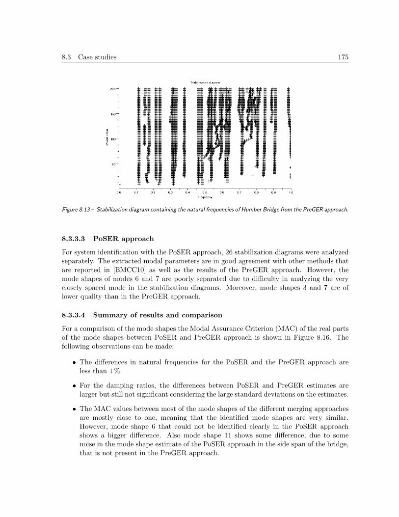
8.3 Case studies 175
Figure 8.13 – Stabilization diagram containing the natural frequencies of Humber Bridge from the PreGER approach.
8.3.3.3 PoSER approach
For system identification with the PoSER approach, 26 stabilization diagrams were analyzedseparately. The extracted modal parameters are in good agreement with other methods thatare reported in [BMCC10] as well as the results of the PreGER approach. However, themode shapes of modes 6 and 7 are poorly separated due to difficulty in analyzing the veryclosely spaced mode in the stabilization diagrams. Moreover, mode shapes 3 and 7 are oflower quality than in the PreGER approach.
8.3.3.4 Summary of results and comparison
For a comparison of the mode shapes the Modal Assurance Criterion (MAC) of the real partsof the mode shapes between PoSER and PreGER approach is shown in Figure 8.16. Thefollowing observations can be made:
The differences in natural frequencies for the PoSER and the PreGER approach areless than 1 %.
For the damping ratios, the differences between PoSER and PreGER estimates arelarger but still not significant considering the large standard deviations on the estimates.
The MAC values between most of the mode shapes of the different merging approachesare mostly close to one, meaning that the identified mode shapes are very similar.However, mode shape 6 that could not be identified clearly in the PoSER approachshows a bigger difference. Also mode shape 11 shows some difference, due to somenoise in the mode shape estimate of the PoSER approach in the side span of the bridge,that is not present in the PreGER approach.

176 Chapter 8
mode 1 - 0.116Hz - 2.8% mode 2 - 0.152Hz - 7.8% mode 3 - 0.174Hz - 5.6%
mode 4 - 0.215Hz - 2.5% mode 5 - 0.239Hz - 1.4% mode 6 - 0.309Hz - 1.6%
mode 7 - 0.312Hz - 1.6% mode 8 - 0.381Hz - 1.4% mode 9 - 0.462Hz - 1.0%
mode 10 - 0.481Hz - 1.0% mode 11 - 0.537Hz - 1.0% mode 12 - 0.625Hz - 0.9%
mode 13 - 0.645Hz - 1.4% mode 14 - 0.712Hz - 1.0% mode 15 - 0.808Hz - 0.9%
mode 16 - 0.845Hz - 1.1% mode 17 - 0.908Hz - 0.8% mode 18 - 0.985Hz - 2.3%
Figure 8.14 – Modes identified with data-driven SSI from the modular PreGER approach (Algorithm 4.4).

8.3 Case studies 177
mode 1 - 0.116Hz - 3.1% mode 2 - 0.152Hz - 6.4% mode 3 - 0.172Hz - 3.9%
mode 4 - 0.215Hz - 2.6% mode 5 - 0.239Hz - 1.4% mode 6 - 0.305Hz - 2.1%
mode 7 - 0.312Hz - 1.2% mode 8 - 0.381Hz - 1.2% mode 9 - 0.462Hz - 0.9%
mode 10 - 0.480Hz - 0.7% mode 11 - 0.537Hz - 0.9% mode 12 - 0.625Hz - 0.7%
mode 13 - 0.647Hz - 0.6% mode 14 - 0.716Hz - 0.7% mode 15 - 0.808Hz - 1.0%
mode 16 - 0.850Hz - 0.7% mode 17 - 0.909Hz - 0.6% mode 18 - 0.987Hz - 0.8%
Figure 8.15 – Modes identified with data-driven SSI from the PoSER approach.

178 Chapter 8
Figure 8.16 – MAC values between the real parts of the mode shapes obtained by PoSER and PreGER approach.
8.3.4 Heritage Court Tower
Within the collaboration with Structural Vibration Solutions A/S (Denmark) the mergingmethods from Chapter 4 were implemented in the commercial software ARTeMIS ExtractorPro [Str11]. A comparative study on a benchmark example in ARTeMIS, the Heritage CourtTower, was made between the classical PoSER and the new PreGER merging approach.
8.3.4.1 Description of the Heritage Court Tower and vibration measurements
The building considered in this study is the Heritage Court Tower (HCT) in downtownVancouver, British Columbia in Canada. It is a relatively regular 15-story reinforced concreteshear core building. In plan, the building is essentially rectangular in shape with only smallprojections and setbacks. Typical floor dimensions of the upper floors are about 25 m by31 m, while the dimensions of the lower three levels are about 36 m by 30 m. The footprintof the building below ground level is about 42 m by 36 m. Typical story heights are 2.70 m,while the first story height is 4.70 m. The elevator and stairs are concentrated at the centercore of the building and form the main lateral resisting elements against potential wind andseismic lateral and torsional forces. The tower structure sits on top of four levels of reinforcedconcrete underground parking. The parking structure extends approximately 14 m beyondthe tower in the south direction forming an L-shaped podium.
As reported in [VBDA01], a series of ambient vibration tests was conducted on April 28,1998 by researchers from the University of British Columbia [DV98]. The vibration measure-ments were conducted using an eight-channel system (with force-balanced accelerometers)and were recorded in four different measurement setups. The accelerometers were typicallylocated in the northwest and northeast corners of the building on every other floor startingfrom the roof down to the ground floor. Details of the field testing of this structure are given

8.3 Case studies 179
in [DV98].The tower model was simplified to a rectangle with nodes aligned vertically. The motions
of the corners of this rectangle were computed from the measured motions by assuming rigidbody motion of the floor slabs. The number of samples was 6560 and hence relatively low,amounting to 328 s at a sampling rate of 20 Hz.
Figure 8.17 – HCT Building and setup close up.
8.3.4.2 Modal analysis with the PoSER and PreGER approaches
The modal analysis for both the PoSER and PreGER approach was tuned with the sameparameters. The maximal considered model order was 80. The parameters for the modalextraction from the stabilization diagrams in ARTeMIS are shown in Figure 8.18.
Figure 8.18 – Parameters of mode extraction from the stabilization diagram.

180 Chapter 8
Figure 8.19 – PoSER stabilization diagram of first setup (top) and PreGER stabilization diagram (bottom).

8.3 Case studies 181
The resulting stabilization diagrams are shown in Figure 8.19. As in previous studies[VBDA01], 6 modes were identified in the frequency range of interest [0–6 Hz]. Their naturalfrequencies and damping ratios are displayed in Table 8.2.
The mode shapes obtained by the PoSER and PreGER approaches are shown in Figure8.20 and a MAC comparison between them is shown in Figure 8.21. The MAC values arevery close to 1, indicating very similar mode shapes.
Table 8.2 – Frequencies (f) and damping coefficients (ρ) of obtained modes with both merging approaches.
PoSER PreGER
Mode f (Hz) ρ (%) f (Hz) ρ (%)
1 1.228 2.04 1.229 2.91
2 1.286 1.90 1.295 2.47
3 1.453 1.35 1.449 1.52
4 3.859 1.26 3.855 1.49
5 4.260 1.50 4.258 2.24
6 5.350 1.84 5.369 2.93
mode 1 mode 2 mode 3
mode 4 mode 5 mode 6
Figure 8.20 – First 6 mode shapes obtained with the PoSER (left in each figure) and the PreGER approach (right)of HCT.

182 Chapter 8
Figure 8.21 – MAC between mode shapes of HCT estimated by PoSER and PreGER approaches.
8.3.5 S101 Bridge
In a collaboration with the University of Tokyo, the system identification of the S101 Bridgewas investigated within the IRIS project. Data-driven SSI with PoSER and PreGER mergingapproaches as well as system identification based on NExT-ERA with a frequency mergingapproach from [SF09] was compared.
8.3.5.1 Description of S101 Bridge and ambient vibration test
The tested bridge is the S101 Overpass Bridge located in Reibersdorf, Upper Austria west sideof Vienna, Austria [SNF+10]. The bridge crossed over the national highway A1 WestautobahnAustria. It is a post-tensioned concrete bridge with the main span of 32 m, side spans of 12 m,and the width of 6.6 m (Figure 8.22). The deck is continuous over the piers and is built into
Figure 8.22 – S101 Bridge and sensor configuration.
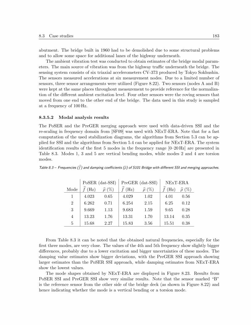
8.3 Case studies 183
abutment. The bridge built in 1960 had to be demolished due to some structural problemsand to allow some space for additional lanes of the highway underneath.
The ambient vibration test was conducted to obtain estimates of the bridge modal param-eters. The main source of vibration was from the highway traffic underneath the bridge. Thesensing system consists of six triaxial accelerometers CV-373 produced by Tokyo Sokhushin.The sensors measured accelerations at six measurement nodes. Due to a limited number ofsensors, three sensor arrangements were utilized (Figure 8.22). Two sensors (nodes A and B)were kept at the same places throughout measurement to provide reference for the normaliza-tion of the different ambient excitation level. Four other sensors were the roving sensors thatmoved from one end to the other end of the bridge. The data used in this study is sampledat a frequency of 100 Hz.
8.3.5.2 Modal analysis results
The PoSER and the PreGER merging approach were used with data-driven SSI and there-scaling in frequency domain from [SF09] was used with NExT-ERA. Note that for a fastcomputation of the used stabilization diagrams, the algorithms from Section 5.3 can be ap-plied for SSI and the algorithms from Section 5.4 can be applied for NExT-ERA. The systemidentification results of the first 5 modes in the frequency range [0–20 Hz] are presented inTable 8.3. Modes 1, 3 and 5 are vertical bending modes, while modes 2 and 4 are torsionmodes.
Table 8.3 – Frequencies (f) and damping coefficients (ρ) of S101 Bridge with different SSI and merging approaches.
PoSER (dat-SSI) PreGER (dat-SSI) NExT-ERA
Mode f (Hz) ρ (%) f (Hz) ρ (%) f (Hz) ρ (%)
1 4.023 0.65 4.029 1.02 4.01 0.56
2 6.262 0.71 6.254 2.15 6.25 0.12
3 9.669 1.13 9.683 1.59 9.65 0.28
4 13.23 1.76 13.31 1.70 13.14 0.35
5 15.68 2.27 15.83 3.56 15.51 0.38
From Table 8.3 it can be noted that the obtained natural frequencies, especially for thefirst three modes, are very close. The values of the 4th and 5th frequency show slightly biggerdifferences, probably due to a lower excitation and bigger uncertainties of these modes. Thedamping value estimates show bigger deviations, with the PreGER SSI approach showinglarger estimates than the PoSER SSI approach, while damping estimates from NExT-ERAshow the lowest values.
The mode shapes obtained by NExT-ERA are displayed in Figure 8.23. Results fromPoSER SSI and PreGER SSI show very similar results. Note that the sensor marked “B”is the reference sensor from the other side of the bridge deck (as shown in Figure 8.22) andhence indicating whether the mode is a vertical bending or a torsion mode.
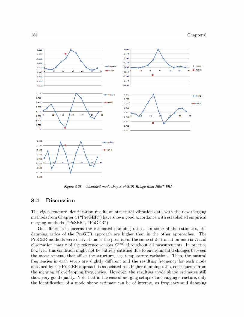
184 Chapter 8
Figure 8.23 – Identified mode shapes of S101 Bridge from NExT-ERA.
8.4 Discussion
The eigenstructure identification results on structural vibration data with the new mergingmethods from Chapter 4 (“PreGER”) have shown good accordance with established empiricalmerging methods (“PoSER”, “PoGER”).
One difference concerns the estimated damping ratios. In some of the estimates, thedamping ratios of the PreGER approach are higher than in the other approaches. ThePreGER methods were derived under the premise of the same state transition matrix A andobservation matrix of the reference sensors C(ref) throughout all measurements. In practicehowever, this condition might not be entirely satisfied due to environmental changes betweenthe measurements that affect the structure, e.g. temperature variations. Then, the naturalfrequencies in each setup are slightly different and the resulting frequency for each modeobtained by the PreGER approach is associated to a higher damping ratio, consequence fromthe merging of overlapping frequencies. However, the resulting mode shape estimates stillshow very good quality. Note that in the case of merging setups of a changing structure, onlythe identification of a mode shape estimate can be of interest, as frequency and damping

8.5 Conclusions 185
values change [PMDR01, BBMN09].The quality of the obtained mode shapes from the PreGER approach is for all case studies
comparable to other merging approaches. However, for closely spaced modes, identificationresults were improved: mode shape estimates identified with PreGER were clearly separated.
The PreGER approach is automated and yields one set of global modal parameters.Thus, no problems arise in analyzing many setups separately and matching identificationresults as in the PoSER approach, which usually also needs user interaction. As only onestabilization diagram needs to computed and analyzed, it is faster. Moreover, it is modular,processing setup after setup, and with its iterative computation, possible memory problemscan be avoided. The PreGER approach is theoretically sound and avoids post-processing ofthe results.
8.5 Conclusions
In this chapter, the new merging algorithms of Chapter 4 were successfully applied to themodal analysis of several large-scale vibrating structures, thus validating their theoreticalderivation. Compared to other established merging methods, they have proven very efficientand gave good results, both with covariance- and data-driven SSI.
Furthermore, first studies on the uncertainty quantification of the obtained eigenstructureidentification results have been made [DLM11, DLAM11].
8.6 Dissemination
Parts of this chapter have been published in:
[DAM10] M. Dohler, P. Andersen, and L. Mevel. Data merging for multi-setup op-erational modal analysis with data-driven SSI. In Proc. 28th InternationalModal Analysis Conference, Jacksonville, FL, USA, 2010.
[DJMB11] M. Dohler, B. Jaishi, L. Mevel, and J.M.W. Brownjohn. Data fusion forsystem identification of the Humber Bridge. In Proc. 29th InternationalModal Analysis Conference, Jacksonville, FL, USA, 2011.
[DRM+10] M. Dohler, E. Reynders, F. Magalhaes, L. Mevel, G. De Roeck, and A. Cunha.Pre- and post-identification merging for multi-setup OMA with covariance-driven SSI. In Proc. 28th International Modal Analysis Conference, Jack-sonville, FL, USA, 2010.
[DSM10] M. Dohler, D. Siringoringo, and L. Mevel. System identification under differ-ent ambient excitations. In Proc. 3rd Asia-Pacific Workshop on StructuralHealth Monitoring, Tokyo, Japan, 2010.

186 Chapter 8
[LPD+10] M. Luczak, B. Peeters, M. Dohler, L. Mevel, W. Ostachowicz, P. Malinowski,T. Wandowski, and K. Branner. Damage detection in wind turbine bladepanels using three different SHM techniques. In Proc. 28th InternationalModal Analysis Conference, Jacksonville, FL, USA, 2010.

Chapter 9
Damage detection and localization
9.1 Introduction
The statistical subspace-based fault detection test was introduced in Section 2.3. It hasbeen proven to be useful for Structural Health Monitoring (SHM) of civil structures, whoseunderlying mechanical model was introduced in Section 2.4. For SHM, the parameters ofthe test (left null space S, covariance Σ, Jacobian J ) are set up in a reference period, wherethe structure is known to be safe. In the monitoring period, values of a χ2-test statistics arecomputed and compared with a threshold to trigger an alarm.
The developments in this thesis are as follows for damage detection and localization. InSection 3.5, numerical improvements of the damage detection test were made regarding itsapplicability to real data. In Chapter 6, this damage detection test is extended to be robustto a changing ambient excitation. In Chapter 7, extensions to damage localization, i.e. to thechange detection in the structural parameters were made, which take into account the mutualinfluence of structural parameters in the test and do not require a finite element model.
In the current chapter, the damage detection test is applied to a real large-scale structureduring progressive artificial damage in order to validate its performance using the improve-ments of Section 3.5. This work was done in collaboration with the German Federal Institutefor Materials Research and Testing (BAM). Also, the rejection of the mutual influence ofstructural parameters for damage localization (Chapter 7) is shown on a large-scale simu-lated bridge deck. Due to the lack of data for the damage detection test under a changingambient excitation (Chapter 6), we refer to Section 6.6 for its application to a mass-springmodel.
This chapter is organized as follows. In Section 9.2, the damage detection test is appliedto vibration data from the progressive damage test of S101 Bridge and compared with systemidentification results of the monitoring data. The damage localization test is applied to asimulated bridge deck in Section 9.3.

188 Chapter 9
9.2 Progressive damage test of S101 Bridge
Within the European research project “Integrated European Industrial Risk Reduction Sys-tem (IRIS)” the prestressed concrete bridge S01 was artificially damaged [VCE09]. Thedamaging processes were accompanied by a permanent measurement of the static and dy-namic behavior of the structure. Like this, a complete record of monitoring data during adefined loss of structural integrity on a typical bridge structure could be provided to test andevaluate SHM methods and applications. Note that the measurements used in this sectionare different from the setting in Section 8.3.5.
In order to validate its performance on a real structure, the damage detection test definedin Section 2.3 is applied to vibration data from the progressive damage test of S101 Bridge.As the implementation of the test in practice raises some numerical problems, the improvedcomputation of the χ2-test statistics for practical problems in Section 3.5 was taken intoaccount.
9.2.1 The S101 Bridge
The S101 was a prestressed concrete bridge from the early 1960th spanning over the 4-lanehighway A1 in Austria (Figure 9.1). The structural system was a three-field frame with a32 m wide mean field and two 12 m wide side fields. The superstructures cross section wasdesigned as a 7.2 m wide post-tensioned double T-beam with varying heights (Figure 9.2).
During recurring technical inspections of the bridge several deficiencies as cracks andspellings have been found. Since the crack pattern correlated with the geometric propertiesof the prestressing a significant deficit of structural reliability was assumed. Because of thesubsequent determined limited load bearing capacity it was decided to replace the structure.
Figure 9.1 – S101 Bridge during damage test [VCE09].

9.2 Progressive damage test of S101 Bridge 189
Figure 9.2 – System drawing of S101 Bridge [VCE09].
9.2.2 Damage description
The damage test took place from 10-13 December 2008. During the test the highway beneaththe bridge was open in one direction. The second direction was closed for traffic because ofconstruction work which in addition took place near the bridge.
Two major damage scenarios were artificially induced. First, a significant damage of oneof the four columns was inserted by cutting through the column on its lower end. Withthis action a change in the global structural system was implemented. After a second cuta 5 cm thick slice of the column was removed and the column was lowered for altogether
Figure 9.3 – Destructive damaging; a) cutting through one of the columns, b) and c) successive intersecting ofprestressing tendons [VCE09].
Table 9.1 – Damage scenarios during progressive damage test of S101 Bridge.
A First cut through column G Uplifting column
B Second cut through column H Exposing cables and cut through first cable
C Lowering column (first step) I Cut through second cable
D Lowering column (second step) J Cut through third cable
E Lowering column (third step) K Cut through fourth cable
F Inserting steel plates
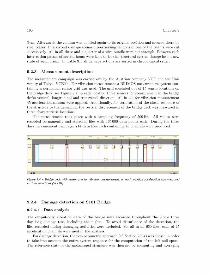
190 Chapter 9
3 cm. Afterwards the column was uplifted again to its original position and secured there bysteel plates. In a second damage scenario prestressing tendons of one of the beams were cutsuccessively. All in all three and a quarter of a wire bundle were cut through. Between eachintersection pauses of several hours were kept to let the structural system change into a newstate of equilibrium. In Table 9.1 all damage actions are sorted in chronological order.
9.2.3 Measurement description
The measurement campaign was carried out by the Austrian company VCE and the Uni-versity of Tokyo [VCE09]. For vibration measurement a BRIMOS measurement system con-taining a permanent sensor grid was used. The grid consisted out of 15 sensor locations onthe bridge deck, see Figure 9.4, in each location three sensors for measurement in the bridgedecks vertical, longitudinal and transversal direction. All in all, for vibration measurement45 acceleration sensors were applied. Additionally, for verification of the static response ofthe structure to the damaging, the vertical displacement of the bridge deck was measured inthree characteristic locations.
The measurement took place with a sampling frequency of 500 Hz. All values wererecorded permanently and stored in files with 165 000 data points each. During the threedays measurement campaign 714 data files each containing 45 channels were produced.
Figure 9.4 – Bridge deck with sensor grid for vibration measurement, on each location acceleration was measuredin three directions [VCE09].
9.2.4 Damage detection on S101 Bridge
9.2.4.1 Data analysis
The output-only vibration data of the bridge were recorded throughout the whole threeday long damage test, including the nights. To avoid disturbance of the detection, thefiles recorded during damaging activities were excluded. So, all in all 660 files, each of 45acceleration channels were used in the analysis.
For damage detection, the non-parametric approach (cf. Section 2.3.4) was chosen in orderto take into account the entire system response for the computation of the left null space.The reference state of the undamaged structure was then set by computing and averaging

9.2 Progressive damage test of S101 Bridge 191
the covariance-driven subspace matrices from several datasets in the reference state, fromwhere the left null space S and the residual covariance Σ were obtained. With this approach,a possible disturbance by single excitation events or different environmental conditions isminimized. For computing the residual covariance matrix 100 datasets of the undamagedstate were used.
In the test stage, the χ2-test statistics is computed for every data set, which in real timemeans an indicator of damage for every 5.5 min.
9.2.4.2 Results
Figure 9.5 shows a bar plot of values as damage indicators of all consecutive tests withinthe three days campaign. The associated analysis used the covariance-driven SSI with allr = r0 = 45 sensors. The abscissa of the plot describes the chronological sequence of thedamage activities as noted in Table 9.1 as well as the 6am and 6pm points of time fororientation. Figure 9.6 shows the damage indicator during the several steps of the firstdamage scenario, the cutting and settling of one of the four bridge columns. With exceptionof the time periods of the direct mechanical destruction processes, which were excluded forcontaining strong noise, the displayed sequence of damage indicators has a consecutive course.
As can be seen in Figure 9.6, the three steps of the column settlement action are verydistinctive in influencing the computed damage indicator. Obviously, the dynamic system haschanged to quite some extend and the altogether 27 mm of elastic settlement can be detectedclearly. Although not that distinctively visible, the cutting of the column (A+B) also causedan increase of the indicator of approximately 75%. However it has to be mentioned that theabsolute effect is superimposed by noise effects. The inlet in Figure 9.6 shows a detail of thattime period.
The column remained in the settled condition for approximately one day and was thenuplifted again in its former position. The effect of the uplifting is again clearly visible inFigure 9.5 by a drop of the damage indicator. However, the χ2-test did not drop completelyto its original value, which is certainly due to the fact that the lowering of one column hasled to cracking within the concrete structure to some extend and therefore also to a changeof the dynamic signature of the system.
The use of so-called reference sensors or projection channels when computing the subspacematrices for the residual reduced the necessary memory and computational cost massively.The analysis using all 45 channels required an extent of memory space which is usually notprovided on desktop computers.
Several numbers and constellations of projection channels were analyzed. Figure 9.7shows a χ2-value plot for only r0 = 4 (instead of 45) projection channels, one vertical andone sensor with all three directions. Note that in the computation of the subspace matrixstill all r = 45 sensors are used, cf. (2.2.3). As one can see, almost equal information aboutthe damage indication could be achieved compared to Figure 9.5, and at the same calculationthe computing time was cut to a fifth compared to a complete sensor analysis.

192 Chapter 9
Figure 9.5 – χ2-test results over the 3-day damage test.
Figure 9.6 – χ2-test for cutting and settling of one bridge column, detail of damage indicator for cutting throughone bridge column.
Figure 9.7 – χ2-test results using r0 = 4 projection channels.

9.2 Progressive damage test of S101 Bridge 193
9.2.5 Comparison to system identification results
9.2.5.1 Data analysis
System identification results of the S101 Bridge were obtained with covariance- and data-driven SSI. In order to compare results at the different damage states, confidence intervalson the obtained results were computed on the results based on [RPDR08]. The algorithmin [RPDR08] was derived for covariance-driven SSI and is extended to data-driven SSI usingthe covariance derivations in Section 3.5.2.
The system identification is done for the first five modes in the frequency range [0–18 Hz].The data was downsampled from the original sampling rate 500 Hz by factor 8 and after a firstexamination only the sensors in vertical direction were chosen, as in this frequency range onlyvertical bending and torsional modes were present. For system identification and confidenceinterval computation the parameters p + 1 = q = 11 were chosen for the subspace matricesand the system orders n = 1, . . . , 70 were considered for stabilization diagrams. Confidencebounds were obtained by cutting the data into 100 blocks.
9.2.5.2 System identification in reference state
In Figure 9.8, the stabilization diagrams of the natural frequencies from both SSI methodsare presented, where the confidence interval of each frequency is plotted as a horizontal bar.The obtained confidence bounds on the frequencies were used to clean the diagrams: Modeswith frequencies having big confidence bounds are likely to be spurious and are erased. In thiscase, all modes with confidence bounds bigger than 2% of the frequency value were deleted.
From the stabilization diagrams, the modes of the system are chosen. In Table 9.2, anoverview of the obtained modal parameters and their confidence bounds at model order 40is given. Note that all confidence bounds are relative values in percent, i.e. the standarddeviation of a value divided by the value and multiplied by 100.
Table 9.2 – Overview of the estimated first 5 modes of S101 Bridge with natural frequencies f , their relativeconfidence bounds σf = σf/f · 100, the damping ratios ρ and their relative confidence bounds σd = σρ/ρ · 100.
Covariance-driven SSI Data-driven SSI (UPC)
mode f (in Hz) σf ρ (in %) σρ f (in Hz) σf ρ (in %) σρ
1 4.039 0.34 1.1 23 4.031 0.21 1.3 22
2 6.292 0.19 0.6 52 6.282 0.11 0.7 19
3 9.730 3.42 3.0 92 9.872 1.17 2.1 32
4 13.19 0.67 1.3 73 13.31 0.38 1.4 22
5 15.72 0.70 1.8 20 15.73 0.39 1.8 19

194 Chapter 9
Figure 9.8 – Stabilization diagrams with covariance-driven SSI (left) and data-driven SSI (right) containing confi-dence intervals on the frequencies (top: full diagrams, bottom: zoom on first mode).
9.2.5.3 Frequency monitoring during damage test
An automated monitoring procedure was applied to each available dataset, which did thesystem identification and a confidence interval computation based on [RPDR08] automaticallyfor each dataset. For each dataset a stabilization diagram was built with the SSI algorithms,containing model orders from 10 to 70. Then, the modes were chosen automatically usingstabilization criteria such as thresholds for the damping estimates and confidence intervalbounds, small frequency deviation between successive model orders, a minimum number ofappearances of a frequency in the diagram and the MAC value between successive modelorders.
The results of the frequency monitoring of all datasets are displayed in Figure 9.9 andthe respective damage scenarios were explained in Table 9.1. Especially the frequency dropcan be clearly seen when one column of the bridge was lowered before it was lifted up again(between A and G). This affected mainly the second, third and fourth mode, while thefrequency changes in the first mode were less important. Especially the change in the fourthmode is remarkable, as it split in two modes during the lowering of the column, with onelower and one higher frequency than before. The frequency changes in the fifth mode cannotbe evaluated, as its uncertainty is very high compared to the other modes.

9.2 Progressive damage test of S101 Bridge 195
(a) covariance-driven SSI
(b) data-driven SSI (UPC)
Figure 9.9 – Natural frequencies with confidence bounds during progressive damage test of S101 Bridge (damageincidents from Table 9.1). The color bar indicates the confidence bound in percent of the obtained frequency.

196 Chapter 9
9.2.6 Discussion
With the statistical damage detection test, the change in the system response of the entirestructure is evaluated. The link between the structural changes due to the artificially in-troduced damage cutting/lowering of one column and the behavior of the respective χ2-testvalues at each test stage was clearly shown. Besides, a significant increase of the efficiency ofthe damage detection test was achieved by the use of projection channels.
Both the covariance- and data-driven SSI give practically identical estimates for systemidentification in this test case, when taking the obtained confidence bounds into account.However, the data-driven approach seems to yield frequency and damping estimates that havelower confidence bounds than the covariance-driven approach. Also, the damage scenarios“cutting/lowering of one column” could be clearly linked to changes in the natural frequencies.
9.3 Damage localization on a simulated bridge deck
The damage localization approach from Chapter 7 is demonstrated on a simulated bridgedeck used in [BBM+08]. The emphasis here lies on the rejection approach (Section 7.3) inorder to avoid the mutual influence of the clustered structural parameters in the associatedχ2-tests. The FE model-free localization approach is not considered in this section.
The FE model and the data of the bridge deck were provided by E. Balmes, SD Tools[BL06], which is gratefully acknowledged.
9.3.1 Finite element model of bridge deck
The data of the bridge deck and the sensitivities with respect to the stiffness parametersof the structural elements are obtained from a finite element model. The FE model of thebridge deck consists of 28 supports and a deck with height 3 m, width 6.6–10 m and length100 m. The whole bridge span is modeled using 9600 standard 8-node isoparametric volumeelements and 13 668 nodes [BBM+08]. A simplified model of the deck with 21 sensor positionis illustrated in Figure 9.10.
Figure 9.10 – Simplified model of the simulated bridge deck.

9.3 Damage localization on a simulated bridge deck 197
Figure 9.11 – The damaged area in the bridge.
In both the undamaged and damaged case, data at the 21 sensor positions was generatedwith a sampling frequency of 256 Hz, where each signal contains 100 000 data samples. Dam-age is introduced by the reduction of the material modulus of up to 30% in 44 elements asillustrated in Figure 9.11.
9.3.2 Damage localization
In the reference state, all the parameters of the χ2-tests for damage localization (see Sec-tions 7.2.3–7.2.4) need to be set up. From the FEM, the modal signature θFE is available,containing the first four modes (frequencies and mode shapes at the 21 measured coordi-nates). Furthermore, the sensitivities ∂θFE/∂pk, k = 1, . . . , P , with respect to the P = 9600structural elements are available. Then, the following steps are done:
1. System identification from data of reference state with covariance-driven SSI – com-putation of modal signature θ0 containing the same modes as θFE (but with possiblyslightly different values as θ0 is computed from data);
2. Computation of left null space S(θ0) from parametric observability matrix O(θ0) andcomputation of the residual covariance Σ;
3. Computation of the residual sensitivity J (θFE) with respect to the modal parameters,using the scaled mode shapes from the FEM; and computation of the sensitivitiesJk = J (θFE)∂θFE/∂pk, k = 1, . . . , P , with respect to the structural parameters;
4. Computation of the change directions dk, k = 1, . . . , P , and clustering them with somecluster algorithm (Sections 7.3.2–7.3.3).
Note that the scaling of the mode shapes for the computation of the residual sensitivity withrespect to the modal parameters J (θ0) (here J (θFE)) must be the same as in the computationof the sensitivities ∂θ0/∂pk (here ∂θFE/∂pk) with respect to the structural parameters. With
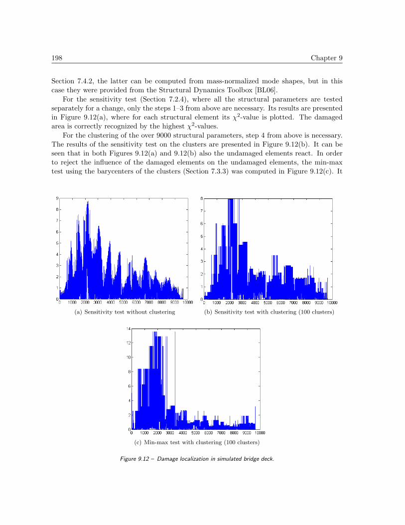
198 Chapter 9
Section 7.4.2, the latter can be computed from mass-normalized mode shapes, but in thiscase they were provided from the Structural Dynamics Toolbox [BL06].
For the sensitivity test (Section 7.2.4), where all the structural parameters are testedseparately for a change, only the steps 1–3 from above are necessary. Its results are presentedin Figure 9.12(a), where for each structural element its χ2-value is plotted. The damagedarea is correctly recognized by the highest χ2-values.
For the clustering of the over 9000 structural parameters, step 4 from above is necessary.The results of the sensitivity test on the clusters are presented in Figure 9.12(b). It can beseen that in both Figures 9.12(a) and 9.12(b) also the undamaged elements react. In orderto reject the influence of the damaged elements on the undamaged elements, the min-maxtest using the barycenters of the clusters (Section 7.3.3) was computed in Figure 9.12(c). It
(a) Sensitivity test without clustering (b) Sensitivity test with clustering (100 clusters)
(c) Min-max test with clustering (100 clusters)
Figure 9.12 – Damage localization in simulated bridge deck.

9.5 Dissemination 199
correctly localizes the damage, but the χ2-values on the undamaged elements are much lower.
9.4 Conclusions
In this chapter, the statistical subspace-based damage detection test was successfully appliedto output-only vibration data from a progressive damage test of the S101 Bridge. Its reac-tivity to artificially introduced damage on a civil structure was shown. An efficient and fastimplementation of the damage detection test was made, which seems to be promising foronline structural health monitoring.
Furthermore, the statistical damage localization was tested on a large-scale simulatedbridge deck, where the rejection of the mutual influence of structural parameters in theχ2-tests showed more contrasted damage localization results. Future work contains the ap-plication of the statistical damage localization on a real structure. Furthermore, the influenceof the clustering on the rejection needs to be explored in detail.
9.5 Dissemination
Parts of this chapter have been published in:
[DHL+11] M. Dohler, F. Hille, X.-B. Lam, L. Mevel, and W. Rucker. Confidence in-tervals of modal parameters during progressive damage test. In Proc. 29thInternational Modal Analysis Conference, Jacksonville, FL, USA, 2011.
[DHMR11] M. Dohler, F. Hille, L. Mevel, and W. Rucker. Structural health monitoringduring progressive damage test of S101 Bridge. In Proc. 8th InternationalWorkshop on Structural Health Monitoring, Stanford, CA, USA, 2011.
[HDMR11] F. Hille, M. Dohler, L. Mevel, and W. Rucker. Subspace based damage de-tection methods on a prestressed concrete bridge. In Proc. 8th InternationalConference on Structural Dynamics (EURODYN), Leuven, Belgium, 2011.
Further applications of the damage detection test are published in [LPS+09, LPD+10,SDBM+10, ZLM+10].

200 Chapter 9

Conclusions
In this thesis, methods for subspace-based system identification as well as fault detection andisolation have been developed, which find an important application in Operational ModalAnalysis of vibrating structures. The developed techniques improve the practical usabilityof established subspace-based methods on real data. The resulting algorithms are faster, nu-merically more robust and can deal with large systems. They take the nature of in-operationdata into account by being robust to changing excitation, noisy data and misspecified modelorder. Their practical relevance was shown on system identification and damage detection ofseveral large-scale civil structures.
The developed methods in this work have a different degree of maturity. The methodson system identification from Part II have been tested extensively on real data from differentlarge-scale structures. Both the multi-setup and the fast multi-order subspace-based systemidentification have been transferred to a commercial software product. The methods fordamage detection and localization from Part III have been successfully tested on simulateddata and still need to be validated on large-scale structures. The validation on structures inthe lab is in progress in collaboration with IFSTTAR and BAM. These methods are also partof the European projects IRIS and ISMS.
A critical discussion of each developed method was made in the respective chapters.Advantages and shortcomings of the new methods can be summarized as follows:
(1) Modular subspace-based system identification from multi-setup measure-ments: A simple, theoretically sound method for global system identification of sys-tems that are measured in multiple setups under possibly varying excitation has beenproposed and successfully applied to the identification of large civil structures. It canbe used with all subspace methods and shows convenient numerical properties. Be-cause of a modular and iterative approach, a large number of sensors and setups can behandled. The merging is done under the assumption that the same system is observedin all the measurement setups. This can be a shortcoming, if the measurements of astructure are taken under different environmental conditions that affect the underlyingsystem itself, such as temperature variations. This might lead to higher estimates ofthe damping ratios, but an effect on the mode shapes was not noticed.
The multi-setup methods were presented with subspace methods using time domaindata, but can directly be adapted to data from the frequency domain with Remark 2.1.Besides, it seems easier to take into account different excitation levels in frequency do-main in order to merge data from multiple setups, which can be done by normalizing
202 Conclusions
cross power spectra [PGC03]. Shifting the approach described in this thesis to the fre-quency domain and comparing it to other frequency domain methods (e.g. [RMDRC09])is a natural extension of this work.
(2) Fast multi-order subspace-based system identification: A fast computationscheme for multi-order subspace-based system identification was proposed, that ac-celerates the computation of stabilization diagrams for structural vibration analysissignificantly. A weak conceptual point might be the necessity of a preprocessing stepat the maximal desired model order, but it was shown that the new method is alreadyfaster when doing the identification at quite low model orders. Note also that the sta-bilization diagram is a standard tool for modal analysis of structures. Thus, the newcomputation scheme finds a wide application. In particular, it can speed up the modalanalysis of online monitoring data significantly.
(3) Robust subspace-based fault detection under changing excitation: Based ona residual function that is robust to changes in the excitation, a modified statisticalsubspace-based fault detection test was proposed. It was shown that the new test doesnot react on a change in the (unmeasured) excitation, but on damage to a simulatedstructure. In the reference state, sufficiently long data sets need to be available, eachrecorded under the same unmeasured excitation, in order to establish the parametersfor a χ2-test. Then, in the possibly damaged state, it can be decided with a very simpleprocedure if the eigenstructure related to the tested data deviates significantly from thereference state or not. In the new method, an additional step is added, which requiresa SVD and its truncation at a chosen model order.
(4) Robust subspace-based damage localization using mass-normalized modeshapes: A statistical damage localization approach was modified to work without afinite element model, but with mass-normalized mode shapes obtained from measure-ments where a known mass perturbation is introduced on the investigated structure.Numerical simulations showed promising properties of this approach, which is probablythe most “experimental” of the presented methods. Note that for damage localization,some extra information needs to be available compared to damage detection – either aFE model, measured excitation of a structure to obtain mass-normalized mode shapes,or in this case a known mass perturbation on the structure. With the rejection schemeof close structural parameters, more contrasted damage localization results were ob-tained. With this approach, a clustering step is necessary for large systems with manyclose structural parameters, which is not necessary without the rejection scheme. Themutual influence of structural parameters needs to be further studied and tested onreal large scale examples.
The rejection approach can in general be used for any kind of parameter that can bemathematically modeled. For example, in [BBMN09] it was used to reject the influenceof the temperature on the stiffness matrix for damage detection robust to temperaturechange. It can be extended in many ways to reject nuisance parameters in damagedetection or localization tests, if an appropriate model exists.

Conclusions 203
With these points, possible areas of further developments of the proposed methods in thisthesis are given.
The subspace-based system identification and fault detection and isolation algorithmsare closely linked: The system matrices and the system’s eigenstructure are identified fromthe subspace matrix. With the detection algorithms, changes in the system’s eigenstructureare detected using the subspace matrix filled with new data. The covariance of the subspacematrix is used for the computation of the residual’s covariance in the fault detection tests, andthe same covariance matrix also leads to the uncertainty quantification of system identificationresults [RPDR08, DLM10a, DHL+11, DLAM11, DLM11]. However, the problem of sizereduction for detection is much more difficult as for identification, as each dimension ofthe involved covariance matrices are of the order of the product of both dimensions of thesubspace matrix. The use of projection channels with r0 r and strategies of Section 3.5.1already increase the feasible problem sizes, and further development should contribute to thisevolution.
The extensive use of numerical tools as QR and SVD decompositions and other matrixcomputations in all parts of this thesis led to improvements of the subspace-based identi-fication and detection algorithms. For example, improvements are robustness to changingexcitation, faster algorithms and, in general, the feasibility of higher problem sizes. This isespecially important for applications in the future, where larger structures are instrumentedwith more and more sensors and problem sizes are continuously increasing. Further employ-ment of numerical techniques and model reduction techniques will probably be needed to dealwith even bigger problem sizes. New technologies as fiber optic sensors, distributed systemsor wireless sensor networks push for this development.
Indeed, the motivation for this thesis was the treatment of large structures under realisticexcitation assumptions for system identification and fault detection. Before this thesis, ithas been shown that subspace methods effectively exhibit great potential to be used forboth identification and fault detection of structures [MHVdA99, MGB03, MBB05, BBGM07].They have interesting properties, such as non-stationary consistency [BM07], the possibilityto reject the temperature effect for damage detection [BBB+08, BBMN09] or the feasibility ofuncertainty quantification of the identification results [RPDR08], but suffered in the contextof large sized case studies. As such, subspace methods had some difficulties with large problemsizes, and several other approaches were once investigated before successfully going back tothe subspace framework.
After over 20 years of the existence of subspace methods, contributions in both theo-retical improvements and practical usability could still be achieved in this thesis. There isfurther room for developments especially for the size explosion regarding subspace-based faultdetection or uncertainty quantification.

204 Conclusions

Resume in French
Introduction
Contexte de la these
L’identification des systemes lineaires et la detection des changements dans les systemes apartir de signaux mesures est une branche de recherche multidisciplinaire dans les champs dela modelisation mathematique, de l’automatique, des statistiques et du traitement du signal.Au cours des dix a vingt dernieres annees, les methodes d’identification des systemes onttrouve un interet particulier dans l’ingenierie des structures pour l’identification des modesvibratoires et de leurs deformees modales, mais egalement pour la detection des changementsdans les caracteristiques de leurs vibrations, dans les deux cas sous conditions operationnelles.Cette analyse modale operationnelle (Operational Modal Analysis, OMA) est composee detrois elements : acquisition de donnees, analyse des donnees collectees et evaluation desresultats. Les avancees dans les systemes d’acquisition des donnees (capteurs moins chers,capteurs a fibre optique, reseaux de capteurs sans fils etc.) conduisent a de plus largessystemes qui peuvent etre surveilles au cours du temps et qui rendent ainsi necessaire undeveloppement plus pousse des techniques statistiques d’analyses de donnees. L’evaluationdes resultats est effectuee par l’ingenieur mecanicien et a par exemple un impact sur laconception des structures, sur le recalage des modeles aux elements finis ou au niveau de ladetection du flottement aeroelastique.
Cette these se situe dans le cadre de l’analyse des donnees, ou l’identification des systemeslineaire ainsi que les methodes de detection des pannes sont utilises. En particulier, dans lecontexte de l’OMA, il est necessaire de prendre en compte les caracteristiques inhabituellessuivantes :
(a) Le nombre de capteurs peut etre eleve (des centaines voire des milliers dans le futur aumoyen de nouvelles technologies). Les capteurs peuvent egalement etre deplaces d’unpoint de mesure a un autre ;
(b) Le nombre de modes peut egalement etre eleve (jusqu’a cent et meme au-dela) et ainsinecessiter des methodes qui peuvent prendre en compte des ordres de modele tres grandsen un temps de calcul raisonnable;
(c) L’excitation appliquee a la structure n’est generalement pas mesuree, pas controlee etaussi turbulente et non stationnaire.

206 Resume in French
Dans cette these, sont developpees des methodes d’identification des systemes et de detectiondes pannes qui prennent en compte les points (a–c) ci-dessus evoques. Les techniquesdeveloppees concernent la theorie de ces methodes, mais tirent leur importance dans le cadrede l’OMA, ou l’analyse de larges structures equipees de nombreux capteurs operant sousconditions bruitees est courante.
Identification des systemes
La conception et la maintenance des structures mecaniques, civiles et aeronautiques soumisesau bruit et aux vibrations sont des sujets particulierement interessants en ingenierie desstructures. Ces elements contribuent au confort, par exemple pour les vehicules et les im-meubles, et contribuent significativement aux aspects securitaires, entre autre pour les avions,les navettes spatiales, les structures civiles, les eoliennes, etc. Il est necessaire de s’assurer quela force dynamique comme le flux de personnes, le trafic, le vent, les vagues ou les seismes,ne compromettent pas le bon fonctionnement de ces structures. Par exemple, la resonanceou le flottement aeroelastique doivent etre evites. Afin d’etudier les proprietes dynamiquesd’une structure, ses modes de vibration (frequences naturelles et taux d’amortissement) etses deformees modales sont analyses.
En consequence, l’identification des modes de vibration et des deformees modales a partirdes donnees mesurees est une etape de base pour l’ingenierie des structures, afin d’etudier etde surveiller les proprietes dynamiques d’une structure. Les caracteristiques des vibrationssont trouvees dans la structure propre d’un systeme lineaire, qui necessite elle d’etre identifieea partir des donnees.
Les methodes pour l’identification des systemes sont souvent issues du domaine del’automatique et se sont averees fonctionner pour des petits ordres des systemes et sousune excitation controlee. Elles ont ete verifiees en theorie, testees sur des donnees simuleeset validees sur des structures artificiellement excitees en laboratoire. L’utilisation de cesmethodes sur des structures de terrain pour l’OMA, ou les caracteristiques (a–c) doiventetre prises en compte, represente la derniere etape dans ce developpement et la principalemotivation de cette these. Dans ce contexte, des techniques sont developpees afin de palier acertains inconvenients de l’identification des systemes dans le contexte de l’OMA.
Detection et diagnostic des pannes
La detection et le diagnostic des pannes sont etablis dans le domaine de l’automatique pourdetecter des conditions anormales de systemes et pour identifier le sous-systeme ou les pannesinterviennent. Applique sur les donnees vibratoires pour des structures reelles, ce principecorrespond a la detection et la localisation des endommagements structurels et est etablipar detection des changements dans les caracteristiques vibratoires ou dans les parametresstructuraux d’une structure. La surveillance des structures (Structural Health Monitoring,SHM) avec de telles methodes permet de surveiller par exemple les infrastructures civiles etaide a identifier les endommagements a un stade precoce.
Le SHM est devenu un champ de recherche important, dans lequel des techniques dedetection non-destructive des endommagements sont utilisees pour surveiller ces structures.

Resume in French 207
De ce fait, les technologies SHM possedent un large potentiel commercial et economique.Elles peuvent aider a identifier les endommagements a un stade precoce, ou des actionscorrectives relativement mineures peuvent etre entreprises au niveau de la structure avantque des deteriorations plus importantes ne surviennent et ne necessitent donc des actionsplus lourdes. La surveillance des endommagements lies aux tremblements de terre representeegalement un exemple d’application SHM. Dans cette situation, le SHM permettrait d’assurerune remise en fonctionnement rapide des infrastructures civiles et des reseaux de transport,ce qui attenuerait l’importance de la perte economique associee a ces evenements sismiques.L’utilisation de SHM dans un contexte de surveillance des infrastructures approchant ou ayantdepasse leur duree de vie initialement prevue, represente egalement un atout certain pour as-surer leur fiabilite et maintenir economiquement des conditions de maintenance raisonnable.D’une maniere generale, il est souhaitable de detecter les endommagements de facon automa-tisee afin de s’affranchir de la necessite des inspections visuelles qui requierent une forte maind’œuvre et qui sont difficiles a realiser dans des environnements a risque ou inaccessibles. Lessystemes SHM permettraient aussi d’integrer les informations apprises lors des constructionsprecedentes afin d’ameliorer la performance des futures structures.
Des methodes pour la detection et le diagnostic des pannes sont issues de la theoriede l’automatique. Elles offrent de prometteuses proprietes et peuvent deja detecter de legerschangements dans la structure propre des systemes lineaires. Neanmoins, pour la detection etla localisation des endommagements pour SHM, les donnees vibratoires sont enregistrees sousdes conditions operationnelles ou les caracteristiques (a–c) ci-dessus evoquees s’appliquent.Ils conduisent a adapter dans le cadre de cette these les methodes actuelles de detectiondes endommagements a de plus realistes hypotheses d’excitation. De plus, la robustessenumerique ainsi que le calcul rapide des indicateurs des endommagements doivent etre assurespour de larges structures sous conditions operationnelles.
Methodes proposees
Il a ete demontre que les methodes d’identification en sous-espace sont efficaces pourl’identification des systemes lineaires invariants comprenant des entrees multiples et sor-ties multiples en utilisant des donnees mesurees sous des conditions d’excitations realistes.Pour l’analyse operationnelle modale des structures vibratoires, il est necessaire d’identifierla structure propre (valeurs propres et vecteurs propres) du systeme lineaire de base a par-tir de laquelle les frequences naturelles, les taux d’amortissement et les deformees modalessont obtenus. La convergence non-stationnaire de nombreuses methodes en sous-espace a eteprouvee pour l’identification de la structure propre, et en fait ainsi des methodes phares pourOMA.
Les methodes suivantes sont developpees dans cette these, ou chacune est motivee par unprobleme pratique de l’OMA :
1. Identification modulaire en sous-espace a partir de mesures multi-sessions,
2. Identification rapide en sous-espace aux ordres de systeme multiples et croissants,

208 Resume in French
3. Detection des pannes robuste aux changements de l’excitation par methodes de sous-espace,
4. Localisation robuste des endommagements par methodes de sous-espace en utilisantdes deformees modales normalisees par rapport a la masse.
D’importantes proprietes theoriques sont etablies pour ces methodes. Elles sont validees surdes donnees vibratoires issues de structures reelles, quand ces donnees sont disponibles. Dansle cas contraire, des donnees simulees sont utilisees afin de valider les methodes.
Chapitre 1 – L’etat de l’art
Dans le domaine de l’identification des systemes, des les annees 1960, des modelesmathematiques des systemes dynamiques sont formules pour des donnees mesureesentree/sortie. Parmi les contributions importantes se trouvent les travaux de Ho etKalman sur le probleme de realisation d’espace d’etat [HK66], ceux d’Astrom et Bohlinsur des methodes de maximum de vraisemblance [AB65], ceux d’Akaike sur la theorie dela realisation stochastique [Aka74c, Aka75], ceux de Ljung sur les methodes d’erreur deprediction [Lju78, LC79] et beaucoup d’autres. Un ouvrage de reference sur l’identificationdes systemes est celui de [Lju99]. Dans [Gev06] se trouve une vue d’ensemble de l’histoire dudeveloppement de la recherche en identification des systemes.
Pour l’identification des systemes lineaires invariants, le modele principal utilise est lemodele d’espace d’etat
Xk+1 = AXk +BUk + Vk+1
Yk = CXk +Wk
avec les etats Xk ∈ Rn, les entrees observees Uk ∈ Rm, les sorties Yk ∈ Rr et les distorsionsnon-observees de l’entree et de la sortie Vk et Wk. L’identification des matrices de systeme Aet C a partir des sorties Yk et des entrees Uk (en cas d’entrees observees) est un des problemesmajeurs en identification des systemes.
La problematique de detection et de diagnostic des pannes (fault detection and isolation,FDI) est de detecter les changements dans les parametres d’un systeme dynamique (detection)et de distinguer les parametres modifies des parametres non-modifies (diagnostic). Il y a denombreuses techniques FDI provenant du domaine de l’automatique [Wil76, PFC89, Fra90,BN93]. En general, ces problemes FDI sont decomposes en deux etapes : 1/ l’obtention d’unresidu qui est dans l’ideal proche de zero en absence de pannes, sensible le moins possibleaux bruits et nuisances, et le plus sensible possible aux pannes ; et 2/ l’evaluation du residu,c’est-a-dire le mise au point des regles de decision basees sur ce residu [Bas98].
Dans ce chapitre, plusieurs contributions de la litterature par rapport a l’identificationdes systemes et la detection des pannes sont presentees.

Resume in French 209
Chapitre 2 – Contexte des methodes sous-espace pourl’identification des systemes et detection des pannes
Les methodes sous-espace pour l’identification des systemes et detection des pannes ainsique leur application a l’analyse des vibrations structurelles constituent le fondement de cettethese. Elles sont expliquees en detail a partir de la litterature dans ce chapitre.
Pour l’identification en sous-espace, une matrice sous-espace H est construite a partir desdonnees mesurees selon un algorithme sous-espace choisi. Avec une decomposition en valeurssingulieres, la matrice d’observabilite O est obtenue, a partir de laquelle les matrices A etC du systeme de l’espace d’etat sont calculees. La structure propre du systeme contient desparametres canoniques et est obtenues a partir des valeurs et vecteurs propres de la matriceA et de la matrice C. Le travail est base sur [BF85, VODM96, PDR99, BM07].
Pour la detection des pannes, des changements dans la structure propre d’un systemelineaire sont detectes en confrontant de nouvelles donnees a un modele de reference dansl’etat sain. Avec l’approche asymptotique locale pour la detection de changements, un residuasymptotique Gaussien est construit en utilisant un noyau gauche obtenu a partir du modelede reference et une matrice sous-espace calculee a partir des donnees dans un etat inconnu eteventuellement en panne. En utilisant un test χ2 sur le residu, une decision peut etre prise sile residu est significativement different de zero indiquant ainsi que le systeme est en panne.Ce travail est base sur [BBM87, BAB00].
L’identification des systemes et la detection des pannes sont souvent appliquees a l’analysede vibrations structurelles. Le modele mecanique de base des structures vibratoires est
M X (t) + C1X (t) +KX (t) = υ(t)
Y (t) = LX (t),
ou t est le temps continu, M , C1 et K sont les matrices de la masse, de l’amortissement et dela raideur, X (t) est le vecteur d’etat qui indique les deplacements aux degres de liberte de lastructure, υ est la force externe non-mesuree, les mesures sont collectees dans le vecteur Y et lamatrice L indique lesquels des degres de liberte sont observes (ou se trouvent des capteurs). Lemodele mecanique peut etre transforme dans un modele discret d’espace d’etat, qui est utilisepour l’identification et la detection. A partir de sa structure propre, les parametres d’interetdu modele mecanique sont obtenus, soient les frequences naturelles, les taux d’amortissementet les deformees modales.
Chapitre 3 – Quelques considerations numeriques pour des al-gorithmes sous-espace
Quelques outils numeriques necessaires pour ce travail sont presentes et derives dans cechapitre. Des proprietes supplementaires de l’algorithme de detection des pannes sontprouvees et eclaircies afin d’augmenter la comprehension theorique de cet algorithme. Deplus, quelques problemes tres pratiques pour le calcul d’un test χ2 associe, concernant letraitement des matrices estimees et a rang deficients, sont resolus. Cette situation apparait

210 Resume in French
quand des ensembles de donnees mesures sur des periodes de temps courtes sont utilises.Une implementation numeriquement robuste est alors proposee. Ces points augmentent enpratique l’applicabilite de l’algorithme de detection
Chapitre 4 – Identification modulaire en sous-espace a partirde mesures multi-sessions
Un des problemes dans le contexte de l’OMA est l’identification de la structure propredes larges structures comme des ponts ou des immeubles. Frequemment, seul un nombrelimite de capteurs est disponible. En consequence, afin d’obtenir des deformees modalesdetaillees malgre une presence limitee de capteurs, des donnees vibratoires d’une structuresont mesurees en plusieurs groupes, ou quelques capteurs restent fixes et d’autres sont deplacesentre les sessions de mesures. En fusionnant ces donnees de differents groupes d’une certainemaniere, l’identification des systemes est possible comme s’il y avait un tres grand nombre decapteurs, allant meme jusqu’a quelques centaines voir milliers. L’excitation entre les sessionspeut varier et l’excitation differente non-mesuree doit etre prise en compte pour fusionnerles donnees. Base sur [MBBG02a, MBBG02b], une approche globale de fusion est proposee,ou dans une premiere etape les donnees de differents groupes sont normalisees et fusionnees,afin d’identifier dans une seconde etape le systeme global. Cette approche est entierementautomatisee et compatible avec toutes les methodes d’identification en sous-espace. Elleest modulaire car les donnees de toutes les sessions sont traitees sequentiellement, et un tresgrand nombre de sessions et capteurs peut etre traite sans se trouver confronte aux problemesde memoire. Pour ses proprietes theoriques, la consistance non-stationnaire et la robustessepar rapport a l’ordre de modele mal specifie sont prouvees, ce qui valide l’utilisation de cetteapproche de fusion sur structure reelle. Elle est appliquee avec succes a plusieurs structuresciviles.
H(1)
H(2)
H(Ns)
O(1,ref), O(1)
O(2)
O(Ns)
......
SVD + re-scaling
SVD + re-scaling
SVD + re-scaling
identificationmergingO(all) f , ρ, ϕ(all)
Figure 1 : Schema de l’approche de fusion developpee (Algorithme 4.4). Dans la premiere etape, les matri-ces d’observabilite sont obtenues a partir des donnees et ensuite normalisees. Apres, elles sont fusionnees pourl’identification globale des systemes.

Resume in French 211
Chapitre 5 – Identification rapide en sous-espace aux ordres desysteme multiples et croissants
Un probleme general pour l’identification de la structure propre d’un systeme dans le con-texte de l’OMA est la distinction entre les vrais modes physiques et les modes parasitesqui apparaissent dans les modeles identifies a cause, entre autre, du bruit colore, des effetsnon-lineaires, de l’excitation non-stationnaire ou d’une specification trop elevee de l’ordre desysteme. D’un autre cote, l’ordre de systeme doit etre presume plus eleve que le nombre demodes presents dans les donnees a cause des effets de bruit. Les modes physiques varient peuen comparant plusieurs estimations a differents ordres de modele tandis que les modes para-sites varient tres fortement, il est donc possible de les distinguer grace a des diagrammes destabilisation, ou les frequences obtenues sont tracees contre les ordres de modele. Pourtant,cette identification aux ordres multiples est couteuse, surtout pour les larges structures oules capteurs sont nombreux et les ordres de systeme eleves. Une procedure de calcul rapideest proposee dans cette these, qui peut etre utilisee avec toutes les methodes d’identificationen sous-espace. Elle reduit le temps de calcul pour l’identification des matrices de systemede O(n4max) a O(n3max), ou nmax est l’ordre de modele maximal. Par exemple, des reductionsdu temps de calcul par facteur 200 ont ete obtenues.
0 50 100 150 200 250 300 350 400 450 50010
−3
10−2
10−1
100
101
102
103
104
maximal model order nmax
com
puta
tiona
l tim
e (s
)
conventional SSI with pseudoinverse (Alg. 5.1)conventional SSI with QR (Alg. 5.1)fast SSI (Alg. 5.2)fast SSI (Alg. 5.3)iterative fast SSI (Alg. 5.4)iterative fast SSI / Householder (Alg. 5.5)
0 50 100 150 200 250 300 350 400 450 50010
−4
10−3
10−2
10−1
100
101
102
103
maximal model order nmax
com
puta
tiona
l tim
e (s
)
conventional SSI with pseudoinverse (Alg. 5.1)conventional SSI with QR (Alg. 5.1)fast SSI (Alg. 5.2)fast SSI (Alg. 5.3)iterative fast SSI (Alg. 5.4)iterative fast SSI / Householder (Alg. 5.5)
Figure 2 : Temps de calcul pour l’identification des matrices de systeme aux ordres multiples 1, 2, . . . , nmax pourdes differents ordres de modele maximal nmax. Les algorithmes 5.2–5.5 sont developpes dans cette these.
Chapitre 6 – Detection des pannes robuste aux changementsde l’excitation par methodes de sous-espace
Avec un test statistique en sous-espace pour la detection des pannes [BAB00], des donneesd’un etat possiblement endommage sont confrontees a un modele de reference en utilisantun test χ2 sur le residu et en comparant le resultat du test a un seuil. En consequence,une decision peut etre prise si la structure propre d’un systeme correspondant aux nouvelles

212 Resume in French
donnees est toujours conforme ou non a la reference, sans identifier la structure propre dansle nouvel etat. En utilisant des donnees de vibrations structurelles, des endommagementsstructurels peuvent etre detectes avec cet algorithme. Dans le contexte de l’OMA, l’excitationambiante n’est pas mesuree et peut varier, par exemple a cause des differences de trafic, devent, etc. Toutefois, un changement de l’excitation a une influence sur la valeur χ2 du test etpeut produire des fausses alarmes. Un nouveau test de detection base sur un residu robusteaux changements dans l’excitation est propose.
0 5 10 15 20 25 30 35 40 45 50
10−4
10−2
100
102
104
#experiment (1−16: reference state, 17−32: 5%, 33−48: 10% stiffness reduction)
χ2 −te
st v
alue
s
Q = I
Q = 42 I
Q = 0.252 I
Q = diag(1,...,6)2
0 5 10 15 20 25 30 35 40 45 5010
−1
100
101
102
103
#experiment (1−16: reference state, 17−32: 5%, 33−48: 10% stiffness reduction)
χ2 −te
st v
alue
s
Q = I
Q = 42 I
Q = 0.252 I
Q = diag(1,...,6)2
Figure 3 : Test de detection des pannes sous des excitations ambiantes differentes avec des donnees simulees. Agauche : test conventionnel, a droite : nouveau test propose dans cette these. Les 16 premieres valeurs χ2 sontcalculees dans le systeme de reference, les 16 valeurs χ2 suivantes sont calculees dans le systeme en panne ou laraideur d’un element a ete baissee de 5%, et les 16 dernieres valeurs χ2 sont calculees avec une baisse de raideurde 10%. Le nouveau test arrive a distinguer clairement les etats de reference des etats en panne.
Chapitre 7 – Localisation robuste des endommagements parmethodes de sous-espace en utilisant des deformees modalesnormalisees par rapport a la masse
Une approche de localisation des endommagements est basee sur la detection des changementsdans les parametres structuraux [BMG04, BBM+08] en utilisant un test χ2. Pour cetteapproche, des sensibilites par rapport aux parametres structuraux, normalement obtenuesd’un modele aux elements finis (finite element model, FEM), sont necessaires. Dans cettethese, une approche sans FEM est proposee, ou les sensibilites necessaires sont obtenuesdes deformees modales normalisees par rapport a la masse. Celles-ci peuvent etre obtenuespar exemple des donnees OMA en utilisant des mesures ou une perturbation connue de lamasse est introduite dans le systeme etudie. De plus, l’influence reciproque des parametresstructuraux dans les tests χ2 est etudiee et un algorithme qui rejette cette influence estpropose. Cela conduit a des resultats plus contrastes dans les tests de localisation entre leselements sains et endommages et contribue a reduire les fausses alarmes.
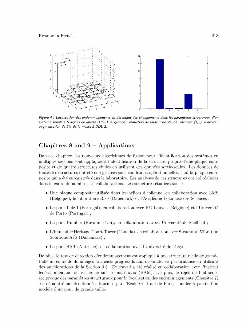
Resume in French 213
Figure 4 : Localisation des endommagements en detectant des changements dans les parametres structuraux d’unsysteme simule a 6 degres de liberte (DDL). A gauche : reduction de raideur de 5% de l’element (1,2), a droite :augmentation de 5% de la masse a DDL 2.
Chapitres 8 and 9 – Applications
Dans ce chapitre, les nouveaux algorithmes de fusion pour l’identification des systemes enmultiples sessions sont appliques a l’identification de la structure propre d’une plaque com-posite et de quatre structures civiles en utilisant des donnees sortie-seules. Les donnees detoutes les structures ont ete enregistrees sous conditions operationnelles, sauf la plaque com-posite qui a ete enregistree dans le laboratoire. Les analyses de ces structures ont ete realiseesdans le cadre de nombreuses collaborations. Les structures etudiees sont :
Une plaque composite utilisee dans les helices d’eolienne, en collaboration avec LMS(Belgique), le laboratoire Risø (Danemark) et l’Academie Polonaise des Sciences ;
Le pont Luiz I (Portugal), en collaboration avec KU Leuven (Belgique) et l’Universitede Porto (Portugal) ;
Le pont Humber (Royaume-Uni), en collaboration avec l’Universite de Sheffield ;
L’immeuble Heritage Court Tower (Canada), en collaboration avec Structural VibrationSolutions A/S (Danemark) ;
Le pont S101 (Autriche), en collaboration avec l’Universite de Tokyo.
De plus, le test de detection d’endommagement est applique a une structure reelle de grandetaille au cours de dommages artificiels progressifs afin de valider sa performance en utilisantdes ameliorations de la Section 3.5. Ce travail a ete realise en collaboration avec l’institutfederal allemand de recherche sur les materiaux (BAM). De plus, le rejet de l’influencereciproque des parametres structuraux pour la localisation des endommagements (Chapitre 7)est demontre sur des donnees fournies par l’Ecole Centrale de Paris, simulee a partir d’unmodele d’un pont de grande taille.

214 Resume in French
mode 1 - 0.116Hz - 2.8% mode 2 - 0.152Hz - 7.8% mode 3 - 0.174Hz - 5.6%
Figure 5 : Les premiers trois modes du pont Humber. Les donnees vibratoires du pont Humber ont ete enregistreesen 26 sessions sous des conditions operationnelles.
Conclusions
Dans cette these, des methodes theoriques ont ete developpees pour l’identification dessystemes ainsi que pour la detection et le diagnostic des pannes, qui s’appliquent a l’analysemodale operationnelle des donnees vibratoires structurelles. Les techniques developpeesameliorent l’applicabilite des methodes sous-espace etablies sur des donnees reelles. Lesalgorithmes resultants sont plus rapides, numeriquement plus robustes et peuvent traiter dessystemes de plus grande dimension. Ils prennent en compte les proprietes intrinseques desdonnees operationnelles en etant robustes aux changements dans l’excitation, aux eventuellesnuisances et a une specification trop elevee de l’ordre de systeme. L’utilisation des outilsnumeriques partout dans cette these, comme les decompositions QR ou SVD et d’autres cal-culs matriciels, a rendu possible ces ameliorations. L’importance pratique des algorithmesdeveloppes a ete demontree pour l’identification des systemes et la detection des endommage-ments de plusieurs structures civiles de grande taille.
Les methodes developpees dans cette these sont de differents degres de maturite. Lesmethodes d’identification des systemes des Chapitres 4 et 5 ont ete testees sur des donneesoperationnelles de differentes structures de grande taille. Les algorithmes pour l’identificationmodulaire en sous-espace a partir de mesures multi-sessions et pour l’identification rapide ensous-espace aux ordres de systeme multiples et croissants ont ete transferes a un logicielcommercial. Les methodes de detection et de localisation des Chapitres 6 et 7 ont ete testeesavec succes sur des donnees simulees et doivent encore etre validees sur des structures degrande taille. Leur validation sur des structures en laboratoire et en cours en collaborationsavec l’IFSSTAR et BAM. Ces methodes font aussi partie des projets europeens IRIS et ISMS.

Bibliography
[AB65] K.J. Astrom and T. Bohlin. Numerical identification of linear dynamic systemsfrom normal operating records. In Proc. IFAC Symposium on Self AdaptiveSystems, Teddington, UK, 1965.
[Akc10] H. Akcay. An insight into instrumental variable frequency-domain subspaceidentification. Automatica, 46(2):375–382, 2010.
[Aka74a] H. Akaike. A new look at the statistical model identification. IEEE Transac-tions on Automatic Control, 19(6):716–723, 1974.
[Aka74b] H. Akaike. Markovian representation of stochastic processes and its applica-tion to the analysis of autoregressive moving average processes. Annals of theInstitute of Statistical Mathematics, 26(1):363–387, 1974.
[Aka74c] H. Akaike. Stochastic theory of minimal realization. IEEE Transactions onAutomatic Control, 19(6):667–674, 1974.
[Aka75] H. Akaike. Markovian representation of stochastic processes by canonicalvariables. SIAM Journal on Control, 13:162–173, 1975.
[AMR09] M. Abdolvahab, L. Mevel, and L. Ramos. Rejection of temperature effectin subspace-based damage monitoring systems: Application to two historicalmonuments. In Proc. 3rd International Operational Modal Analysis Confer-ence, Ancona, Italy, 2009.
[Au11] S.-K. Au. Assembling mode shapes by least squares. Mechanical Systems andSignal Processing, 25(1):163–179, 2011.
[AWDR99] M.M. Abdel Wahab and G. De Roeck. Damage detection in bridges usingmodal curvatures: application to a real damage scenario. Journal of Soundand Vibration, 226(2):217–235, 1999.
[BA03] R. Brincker and P. Andersen. A way of getting scaled mode shapes in outputonly modal testing. In Proc. 21st International Modal Analysis Conference,Kissimmee, Florida, USA, 2003.
216 Bibliography
[BAB97] M. Basseville, M. Abdelghani, and A. Benveniste. Subspace-based fault de-tection and isolation methods - application to vibration monitoring. TechnicalReport 3299, INRIA, 1997.
[BAB00] M. Basseville, M. Abdelghani, and A. Benveniste. Subspace-based fault de-tection algorithms for vibration monitoring. Automatica, 36(1):101–109, 2000.
[Bak11] P.G. Bakir. Automation of the stabilization diagrams for subspace basedsystem identification. Expert Systems with Applications, 38(12):14390–14397,2011.
[Bas97] M. Basseville. Information criteria for residual generation and fault detectionand isolation. Automatica, 33(5):783–803, 1997.
[Bas98] M. Basseville. On-board component fault detection and isolation using thestatistical local approach. Automatica, 34(11):1391–1415, 1998.
[Bas99] M. Basseville. An invariance property of some subspace-based detection algo-rithms. IEEE Transactions on Signal Processing, 47(12):3398–3400, 1999.
[Bau01] D. Bauer. Order estimation for subspace methods. Automatica, 37(10):1561–1573, 2001.
[Bau05] D. Bauer. Asymptotic properties of subspace estimators. Automatica,41(3):359–376, 2005.
[BAZM79] D.L. Brown, R.J. Allemang, R.D. Zimmerman, and M. Mergeay. Parame-ter estimation techniques for modal analysis. SAE Transactions, 88:828–846,1979. SAE Paper Number 689110.
[BB11] D. Bernal and Y. Bulut. A modified whiteness test for damage detectionusing Kalman filter innovations. In Proc. 27th International Modal AnalysisConference, Jacksonville, Fl, USA, 2011.
[BBB+08] E. Balmes, M. Basseville, F. Bourquin, L. Mevel, H. Nasser, and F. Treyssede.Merging sensor data from multiple temperature scenarios for vibration-basedmonitoring of civil structures. Structural Health Monitoring, 7(2):129–142,2008.
[BBG+01] M. Basseville, A. Benveniste, M. Goursat, L. Hermans, L. Mevel, andH. Van der Auweraer. Output-only subspace-based structural identification:from theory to industrial testing practice. Journal of Dynamic Systems, Mea-surement, and Control, 123(4):668–676, 2001.
[BBGM06] A. Benveniste, M. Basseville, M. Goursat, and L. Mevel. The local approachto change detection, diagnosis, and model validation: application to vibrationmechanics. In Torkel Glad, editor, Forever Ljung in system identification- Workshop on the occasion of Lennart Ljung’s 60th birthday, pages 3–35.Studentlitteratur, Lund, SE, 2006.
Bibliography 217
[BBGM07] M. Basseville, A. Benveniste, M. Goursat, and L. Mevel. In-flight monitoring ofaeronautic structures: vibration-based on-line automated identification versusdetection. IEEE Control Systems Magazine, 27(5):27–42, 2007.
[BBM87] A. Benveniste, M. Basseville, and G. Moustakides. The asymptotic local ap-proach to change detection and model validation. IEEE Transactions on Au-tomatic Control, 32(7):583–592, 1987.
[BBM+06] M. Basseville, F. Bourquin, L. Mevel, H. Nasser, and F. Treyssede. Mergingsensor data from multiple temperature scenarios for vibration-based monitor-ing of civil structures. In Proc. 3rd European Workshop on Structural HealthMonitoring, pages 499–506, Granada, Spain, 2006.
[BBM+08] E. Balmes, M. Basseville, L. Mevel, H. Nasser, and W. Zhou. Statistical model-based damage localization: a combined subspace-based and substructuringapproach. Structural Control and Health Monitoring, 15(6):857–875, 2008.
[BBM+10] M. Basseville, F. Bourquin, L. Mevel, H. Nasser, and F. Treyssede. Handlingthe temperature effect in vibration monitoring: two subspace-based analyticalapproaches. Journal of Engineering Mechanics, 136(3):367–378, 2010.
[BBMN09] E. Balmes, M. Basseville, L. Mevel, and H. Nasser. Handling the temper-ature effect in vibration-based monitoring of civil structures: a combinedsubspace-based and nuisance rejection approach. Control Engineering Prac-tice, 17(1):80–87, 2009.
[BDS99] D. Bauer, M. Deistler, and W. Scherrer. Consistency and asymptotic normal-ity of some subspace algorithms for systems without observed inputs. Auto-matica, 35(7):1243–1254, 1999.
[BDST87] J.M.W. Brownjohn, A.A. Dumanoglu, R.T. Severn, and C.A. Taylor. Ambientvibration measurements of the Humber suspension bridge and comparisonwith calculated characteristics. In Proc. of the Institution of Civil Engineers(London), volume 83, pages 561–600, 1987.
[Ber02] D. Bernal. Load vectors for damage localization. Journal of EngineeringMechanics, 128(1):7–14, 2002.
[Ber04] D. Bernal. Modal scaling from known mass perturbations. Journal of Engi-neering Mechanics, 130(9):1083–1088, 2004.
[Ber06] D. Bernal. Flexibility-based damage localization from stochastic realizationresults. Journal of Engineering Mechanics, 132(6):651–658, 2006.
[Ber10] D. Bernal. Load vectors for damage location in systems identified from oper-ational loads. Journal of Engineering Mechanics, 136(1):31–39, 2010.

218 Bibliography
[Ber11a] D. Bernal. Eigenvector normalization from mass perturbations: a review. InProc. International Symposium on Nondestructive Testing of Materials andStructures, Istanbul, Turkey, 2011.
[Ber11b] D. Bernal. Kalman filter detection under variable noise statistics. In Proc. 4thInternational Operational Modal Analysis Conference, Istanbul, Turkey, 2011.
[Ber11c] D. Bernal. The receptance approach to complex operational mode normal-ization. In Proc. 4th International Operational Modal Analysis Conference,Istanbul, Turkey, 2011.
[Ber11d] D. Bernal. A receptance based formulation for modal scaling using mass per-turbations. Mechanical Systems and Signal Processing, 25(2):621–629, 2011.
[BF85] A. Benveniste and J.-J. Fuchs. Single sample modal identification of a non-stationary stochastic process. IEEE Transactions on Automatic Control, AC-30(1):66–74, 1985.
[BG63] R.E.D. Bishop and G.M.L. Gladwell. An investigation into the theory ofresonance testing. Philosophical Transactions of the Royal Society A: Mathe-matical and Physical Sciences, 255(1055):241–280, 1963.
[BL02] D. Bauer and L. Ljung. Some facts about the choice of the weighting matricesin Larimore type of subspace algorithms. Automatica, 38(5):763–773, 2002.
[BL06] E. Balmes and J.-M. Leclere. Structural Dynamics Toolbox, User’s GuideVersion 5.3, SD Tools, 2006.
[BM07] A. Benveniste and L. Mevel. Non-stationary consistency of subspace methods.IEEE Transactions on Automatic Control, AC-52(6):974–984, 2007.
[BMCC10] J.M.W. Brownjohn, F. Magalhaes, E. Caetano, and A. Cunha. Ambient vi-bration re-testing and operational modal analysis of the Humber Bridge. En-gineering Structures, 32(8):2003–2018, 2010.
[BMG04] M. Basseville, L. Mevel, and M. Goursat. Statistical model-based damage de-tection and localization: subspace-based residuals and damage-to-noise sensi-tivity ratios. Journal of Sound and Vibration, 275(3):769–794, 2004.
[BMP90] A. Benveniste, M. Metivier, and P. Priouret. Adaptive Algorithms and Stochas-tic Approximations, volume 22 of Applications of Mathematics. Springer-Verlag, New York, 1990.
[BN93] M. Basseville and I. Nikiforov. Detection of Abrupt Changes - Theory and Ap-plications. Information and System Sciences Series. Prentice Hall, EnglewoodCliffs, NJ, 1993.

Bibliography 219
[BNSR98] T. Bastogne, H. Noura, P. Sibille, and A. Richard. Multivariable identifica-tion of a winding process by subspace methods for tension control. ControlEngineering Practice, 6(9):1077–1088, 1998.
[BP93] J.S. Bendat and A.G. Piersol. Engineering Applications of Correlation andSpectral Analysis. John Wiley & Sons, New York, USA, 2nd edition, 1993.
[BP08] E. Bura and R. Pfeiffer. On the distribution of the left singular vectors of a ran-dom matrix and its applications. Statistics & Probability Letters, 78(15):2275–2280, 2008.
[Bro03] J.M.W. Brownjohn. Ambient vibration studies for system identification of tallbuildings. Earthquake Engineering & Structural Dynamics, 32(1):71–95, 2003.
[Bro11] M. Brookes. The matrix reference manual, 2011. http://www.ee.imperial.ac.uk/hp/staff/dmb/matrix/intro.html.
[BVA01] R. Brincker, C.E. Ventura, and P. Andersen. Damping estimation by fre-quency domain decomposition. In Proc. 19th International Modal AnalysisConference, Kissimmee, FL, USA, 2001.
[BZA01] R. Brincker, L. Zhang, and P. Andersen. Modal identification of output-only systems using frequency domain decomposition. Smart Materials andStructures, 10(3):441–445, 2001.
[CBP06] J. Ching, J.L. Beck, and K.A. Porter. Bayesian state and parameter esti-mation of uncertain dynamical systems. Probabilistic Engineering Mechanics,21(1):81–96, 2006.
[CF04] E.P. Carden and P. Fanning. Vibration based condition monitoring: a review.Structural Health Monitoring, 3(4):355–377, 2004.
[CGDV02] B. Cauberghe, P. Guillaume, B. Dierckx, and P. Verboven. Identification ofmodal parameters from inconsistent data. In Proc. 20th International ModalAnalysis Conference, pages 809–815, Los Angeles, CA, USA, 2002.
[CGPV06] B. Cauberghe, P. Guillaume, R. Pintelon, and P. Verboven. Frequency-domainsubspace identification using FRF data from arbitrary signals. Journal ofSound and Vibration, 290(3-5):555–571, 2006.
[CGV+05] B. Cauberghe, P. Guillaume, P. Verboven, S. Vanlanduit, and E. Parloo. Onthe influence of the parameter constraint on the stability of the poles and thediscrimination capabilities of the stabilisation diagrams. Mechanical Systemsand Signal Processing, 19(5):989–1014, 2005.
[CGVP03] B. Cauberghe, P. Guillaume, P. Verboven, and E. Parloo. Identification ofmodal parameters including unmeasured forces and transient effects. Journalof Sound and Vibration, 265(3):609–625, 2003.

220 Bibliography
[CK95] Y.M. Cho and T. Kailath. Fast subspace-based system identification: Aninstrumental variable approach. Automatica, 31(6):903–905, 1995.
[CMC06] A. Cunha, F. Magalhaes, and E. Caetano. Output-only modal identification ofLuiz I bridge before and after rehabilitation. In Proc. 22th International Con-ference on Noise and Vibration Engineering (ISMA2006), Leuven, Belgium,2006.
[CMK01] G. Camba-Mendez and G. Kapetanios. Testing the rank of the Hankel co-variance matrix: A statistical approach. IEEE Transactions on AutomaticControl, 46(2):331–336, 2001.
[Col68] H.A. Cole. On-the-line analysis of random vibrations. AIAA Paper No. 68-288, 1968.
[CP04a] A. Chiuso and G. Picci. Asymptotic variance of subspace methods by dataorthogonalization and model decoupling: a comparative analysis. Automatica,40(10):1705–1717, 2004.
[CP04b] A. Chiuso and G. Picci. Subspace identification by data orthogonalization andmodel decoupling. Automatica, 40(10):1689–1703, 2004.
[DAM10] M. Dohler, P. Andersen, and L. Mevel. Data merging for multi-setup opera-tional modal analysis with data-driven SSI. In Proc. 28th International ModalAnalysis Conference, Jacksonville, FL, USA, 2010.
[DB97] B. Delyon and A. Benveniste. On the relationship between identification andlocal tests. In Proc. 36th IEEE Conference on Decision and Control, pages139–144, 1997.
[DBMS11] M. Dohler, D. Bernal, L. Mevel, and D. Siegert. Statistical-based model-freedamage localization. In Proc. 4th International Operational Modal AnalysisConference, Istanbul, Turkey, 2011.
[DDSG10] C. Devriendt, G. De Sitter, and P. Guillaume. An operational modal analysisapproach based on parametrically identified multivariable transmissibilities.Mechanical Systems and Signal Processing, 24(5):1250–1259, 2010. SpecialIssue: Operational Modal Analysis.
[DFP98] S.W. Doebling, C.R. Farrar, and M.B. Prime. A summary review of vibration-based damage identification methods. Shock and Vibration Digest, 30(2):91–105, 1998.
[DHL+11] M. Dohler, F. Hille, X.-B. Lam, L. Mevel, and W. Rucker. Confidence in-tervals of modal parameters during progressive damage test. In Proc. 29thInternational Modal Analysis Conference, Jacksonville, FL, USA, 2011.

Bibliography 221
[DHMR11] M. Dohler, F. Hille, L. Mevel, and W. Rucker. Structural health monitoringduring progressive damage test of S101 Bridge. In Proc. 8th InternationalWorkshop on Structural Health Monitoring, Stanford, CA, USA, 2011.
[DJMB11] M. Dohler, B. Jaishi, L. Mevel, and J.M.W. Brownjohn. Data fusion forsystem identification of the Humber Bridge. In Proc. 29th International ModalAnalysis Conference, Jacksonville, FL, USA, 2011.
[DLAM11] M. Dohler, X.-B. Lam, P. Andersen, and L. Mevel. Uncertainty quantificationfor stochastic subspace identification of multi-setup measurements. In Proc.4th International Operational Modal Analysis Conference, Istanbul, Turkey,2011.
[DLM10a] M. Dohler, X.-B. Lam, and L. Mevel. Confidence intervals on modal pa-rameters in stochastic subspace identification. In Proc. 34th InternationalSymposium on Bridge and Structural Engineering, Venice, Italy, 2010.
[DLM10b] M. Dohler, X.-B. Lam, and L. Mevel. Crystal clear data fusion in subspacesystem identification and damage detection. In Proc. 5th International Con-ference on Bridge Maintenance, Safety and Management, Philadelphia, PA,USA, 2010.
[DLM11] M. Dohler, X.-B. Lam, and L. Mevel. Uncertainty quantification for stochasticsubspace identification on multi-setup measurements. In Proc. 50th IEEEConference on Decision and Control, Orlando, FL, USA, 2011.
[DM10] M. Dohler and L. Mevel. Modular subspace-based system identification anddamage detection on large structures. In Proc. 34th International Symposiumon Bridge and Structural Engineering, Venice, Italy, 2010.
[DM11a] M. Dohler and L. Mevel. Fast multi-order stochastic subspace-based systemidentification. 2011. Control Engineering Practice, under revision.
[DM11b] M. Dohler and L. Mevel. Fast multi-order stochastic subspace identification.In Proc. 18th IFAC World Congress, Milan, Italy, 2011.
[DM11c] M. Dohler and L. Mevel. Modular subspace-based system identification frommulti-setup measurements. 2011. IEEE Transactions on Automatic Control,under revision.
[DM11d] M. Dohler and L. Mevel. Robust subspace based fault detection. In Proc. 18thIFAC World Congress, Milan, Italy, 2011.
[DMB11] M. Dohler, L. Mevel, and D. Bernal. Statistical subspace-based model-freedamage localization. In Proc. Engineering Mechanics Institute Conference,Boston, USA, 2011.
[DPS95] M. Deistler, K. Peternell, and W. Scherrer. Consistency and relative efficiencyof subspace methods. Automatica, 31(12):1865–1875, 1995.
222 Bibliography
[DRM+10] M. Dohler, E. Reynders, F. Magalhaes, L. Mevel, G. De Roeck, and A. Cunha.Pre- and post-identification merging for multi-setup OMA with covariance-driven SSI. In Proc. 28th International Modal Analysis Conference, Jack-sonville, FL, USA, 2010.
[DSM10] M. Dohler, D. Siringoringo, and L. Mevel. System identification under differentambient excitations. In Proc. 3rd Asia-Pacific Workshop on Structural HealthMonitoring, Tokyo, Japan, 2010.
[DV98] C. Dyck and C.E. Ventura. Ambient Vibration Measurements of HeritageCourt Tower. EQ LAB, University of British Columbia, Earthquake Engi-neering Research, 1998.
[Ewi84] D.J. Ewins. Modal testing: theory and practice. Research Studies Press Ltd.,Letchworth, Hertfordshire, UK, 1984.
[Fac05] P.L. Fackler. Notes on matrix calculus. Technical report, North Carolina StateUniversity, 2005.
[FDN01] C.R. Farrar, S.W. Doebling, and D.A. Nix. Vibration-based structural damageidentification. Philosophical Transactions of the Royal Society A: Mathemat-ical, Physical and Engineering Science, 359(1778):131–149, 2001.
[Fis05] R.F.H. Fischer. Precoding and Signal Shaping for Digital Transmission, chap-ter Appendix A: Wirtinger Calculus, pages 405–413. John Wiley & Sons, Inc.,2005.
[FJI97] C.R. Farrar and G.H. James III. System identification from ambient vibrationmeasurements on a bridge. Journal of Sound and Vibration, 205(1):1–18, 1997.
[FJK98] C.-P. Fritzen, D. Jennewein, and T. Kiefer. Damage detection based on modelupdating methods. Mechanical Systems and Signal Processing, 12(1):163–186,1998.
[FK09] C.-P. Fritzen and P. Kraemer. Self-diagnosis of smart structures based ondynamical properties. Mechanical Systems and Signal Processing, 23(6):1830–1845, 2009. Special Issue: Inverse Problems.
[FM02] C.-P. Fritzen and G. Mengelkamp. Detection of delaminations in compositematerials using a smart structures concept. In Proc. First European Workshopon Structural Health Monitoring, Paris, France, 2002.
[FMG03] C.-P. Fritzen, G. Mengelkamp, and A. Guemes. Elimination of temperatureeffects on damage detection within a smart structure concept. In Proc. 4thInternational Workshop on Structural Health Monitoring, Stanford, CA, USA,2003.
Bibliography 223
[Fra90] P.M. Frank. Fault diagnosis in dynamic systems using analytical andknowledge-based redundancy: A survey and some new results. Automatica,26(3):459–474, 1990.
[GD91] B. Gach-Devauchelle. Diagnostic Mecanique des Fatigues sur les StructuresSoumises a des Vibrations en Ambiance de Travail (In French). PhD thesis,Universite de Paris IX Dauphine, Paris, FR, 1991.
[Ger74] W. Gersch. On the achievable accuracy of structural system parameter esti-mates. Journal of Sound and Vibration, 34(1):63–79, 1974.
[Gev06] M. Gevers. A personal view of the development of system identification. IEEEControl Systems Magazine, 26(6):93–105, 2006.
[GM03] A. Guyader and L. Mevel. Covariance-driven subspace methods: input/outputvs. output-only. In Proc. 21th International Modal Analysis Conference,Kissimmee, FL, USA, 2003.
[GP96] P. Guillaume and R. Pintelon. A gauss-newton-like optimization algorithm for“weighted” nonlinear least-squares problems. IEEE Transactions on SignalProcessing, 44(9):2222–2228, 1996.
[Gra84] R.M. Gray. Vector quantization. IEEE ASSP Magazine, 1(2):4–29, 1984.
[GS08] H.M. Gomes and N.R.S. Silva. Some comparisons for damage detection onstructures using genetic algorithms and modal sensitivity method. AppliedMathematical Modelling, 32(11):2216–2232, 2008.
[Gus98] T. Gustafsson. Instrumental variable subspace tracking using projection ap-proximation. IEEE Transactions on Signal Processing, 46(3):669–681, 1998.
[GVC+03] P. Guillaume, P. Verboven, B. Cauberghe, S. Vanlanduit, E. Parloo, andG. De Sitter. Frequency-domain system identification techniques for experi-mental and operational modal analysis. In Proc. 13th IFAC Symposium onSystem Identification, Rotterdam, The Netherlands, 2003.
[GVL96] G.H. Golub and C.F. Van Loan. Matrix computations. Johns Hopkins Uni-versity Press, 3rd edition, 1996.
[GVV98] P. Guillaume, P. Verboven, and S. Vanlanduit. Frequency-domain maximumlikelihood identification of modal parameters with confidence intervals. InProc. 24th International Seminar on Modal Analysis (ISMA), 1998.
[GVV+03] P. Guillaume, P. Verboven, S. Vanlanduit, H. Van der Auweraer, andB. Peeters. A poly-reference implementation of the least-squares complexfrequency-domain estimator. In Proc. 21th International Modal Analysis Con-ference, Kissimmee, FL, USA, 2003.

224 Bibliography
[GZ08] M.P. Gonzalez and J.L. Zapico. Seismic damage identification in buildingsusing neural networks and modal data. Computers & Structures, 86(3-5):416–426, 2008.
[HDMR11] F. Hille, M. Dohler, L. Mevel, and W. Rucker. Subspace based damage de-tection methods on a prestressed concrete bridge. In Proc. 8th InternationalConference on Structural Dynamics (EURODYN), Leuven, Belgium, 2011.
[HK66] B.L. Ho and R.E. Kalman. Effective construction of linear state-variable mod-els from input/output functions. Regelungstechnik, 14(12):545–548, 1966.
[HLS98] W. Heylen, S. Lammens, and P. Sas. Modal Analysis Theory and Testing.Katholieke Universiteit Leuven, Belgium, 1998.
[HVdA99] L. Hermans and H. Van der Auweraer. Modal testing and analysis of structuresunder operational conditions: industrial application. Mechanical Systems andSignal Processing, 13(2):193–216, 1999.
[Ibr77] S.R. Ibrahim. Random decrement technique for modal identification of struc-tures. Journal of Spacecraft and Rockets, 14(11):696–700, 1977.
[IM76] S.R. Ibrahim and E.C. Mikulcik. The experimental determination of vibrationparameters from time responses. Shock and Vibration Bulletin, 46(5):187–196,1976.
[JICL95] G.H. James III, T.G. Carne, and J.P. Lauffer. The natural excitation technique(NExT) for modal parameter extraction from operating structures. ModalAnalysis - The International Journal of Analytical and Experimental ModalAnalysis, 10:260–277, 1995.
[JP85] J.-N. Juang and R.S. Pappa. Eigensystem realization algorithm for modalparameter identification and model reduction. Journal of Guidance, Controland Dynamics, 8(5):620–627, 1985.
[JR06] B. Jaishi and W.X. Ren. Damage detection by finite element model updatingusing modal flexibility residual. Journal of Sound and Vibration, 290(1-2):369–387, 2006.
[JSL01] B.C. Juricek, D.E. Seborg, and W.E. Larimore. Identification of the TennesseeEastman challenge process with subspace methods. Control Engineering Prac-tice, 9(12):1337–1351, 2001.
[Jua94] J.-N. Juang. Applied system identification. Prentice Hall, Englewood Cliffs,NJ, USA, 1994.
[KM04] H. Kim and H. Melhem. Damage detection of structures by wavelet analysis.Engineering Structures, 26(3):347–362, 2004.

Bibliography 225
[KS95] J.T. Kim and N. Stubbs. Model-uncertainty impact and damage-detectionaccuracy in plate girder. Journal of Structural Engineering, 121(10):1409–1417, 1995.
[KS02] J.T. Kim and N. Stubbs. Improved damage identification method based onmodal information. Journal of Sound and Vibration, 252(2):223–238, 2002.
[Kul03] J. Kullaa. Damage detection of the Z24 Bridge using control charts. Mechan-ical Systems and Signal Processing, 17(1):163–170, 2003.
[Kun78] S.Y. Kung. A new identification and model reduction algorithm via singularvalue decomposition. In Proc. 12th Asilomar Conference on Circuits, Systems,and Computers, pages 705–714, Pacific Grove, CA, USA, 1978.
[Lar83] W.E. Larimore. System identification, reduced order filters and modellingvia canonical variate analysis. In Proc. American Control Conference, pages445–451, San Francisco, 1983.
[LBG80] Y. Linde, A. Buzo, and R.M. Gray. An algorithm for vector quantizer design.IEEE Transactions on Communications, 28(1):84–95, 1980.
[LC56] L. Le Cam. On the asymptotic theory of estimation and testing hypotheses.In Proc. 3rd Berkeley Symposium on Mathematical Statistics and Probability,pages 129–156, University of California, 1956.
[LC79] L. Ljung and P.E. Caines. Asymptotic normality of prediction error estimatorsfor approximate system models. Stochastics – An International Journal ofProbability and Stochastic Processes, 3(1):29–46, 1979.
[LC86] L. Le Cam. Asymptotic Methods in Statistical Decision Theory. Series inStatistics. Springer, NY, 1986.
[Lju78] L. Ljung. Convergence analysis of parametric identification methods. IEEETransactions on Automatic Control, 23(5):770–783, 1978.
[Lju99] L. Ljung. System identification: theory for the user. Prentice Hall, EnglewoodCliffs, NJ, USA, 1999.
[LPD+10] M. Luczak, B. Peeters, M. Dohler, L. Mevel, W. Ostachowicz, P. Malinowski,T. Wandowski, and K. Branner. Damage detection in wind turbine bladepanels using three different SHM techniques. In Proc. 28th International ModalAnalysis Conference, Jacksonville, FL, USA, 2010.
[LPS+09] M. Luczak, B. Peeters, W. Szkudlarek, L. Mevel, M. Dohler, W. Ostachowicz,K. Martyniuk, and K. Branner. Comparison of the three different approachesfor damage detection in the part of the composite wind turbine blade. In Proc.7th International Workshop on Structural Health Monitoring, Stanford, CA,USA, 2009.
226 Bibliography
[LS10] M. Luczak and W. Szkudlarek. Damage detecting in E-glass composite mate-rial. Technical report, LMS, 2010.
[LW98] K.M. Liew and Q. Wang. Application of wavelet theory for crack identificationin structures. Journal of Engineering Mechanics, 124(2):152–157, 1998.
[MaCC08] F. Magalhaes, A. Cunha, and E. Caetano. Dynamic monitoring of a long spanarch bridge. Engineering Structures, 30(11):3034–3044, 2008.
[MaCC10] F. Magalhaes, A. Cunha, and E. Caetano. Continuous dynamic monitoringof an arch bridge: strategy to eliminate the environmental and operationaleffects and detect damages. In Proc. 24th International Conference on Noiseand Vibration Engineering (ISMA2010), Leuven, Belgium, 2010.
[MAL96] T. McKelvey, H. Akcay, and L. Ljung. Subspace-based multivariable systemidentification from frequency response data. IEEE Transactions on AutomaticControl, 41(7):960–979, 1996.
[MB86] G.V. Moustakides and A. Benveniste. Detecting changes in the AR parametersof a nonstationary ARMA process. Stochastics – An International Journal ofProbability and Stochastic Processes, 16(1):137–155, 1986.
[MBB05] L. Mevel, M. Basseville, and A. Benveniste. Fast in-flight detection of flut-ter onset: a statistical approach. AIAA Journal of Guidance, Control, andDynamics, 28(3):431–438, 2005.
[MBB+06] L. Mevel, A. Benveniste, M. Basseville, M. Goursat, B. Peeters, H. Van derAuweraer, and A. Vecchio. Input/output versus output-only data processingfor structural identification - application to in-flight data analysis. Journal ofSound and Vibration, 295(3):531–552, 2006.
[MBBG02a] L. Mevel, M. Basseville, A. Benveniste, and M. Goursat. Merging sensor datafrom multiple measurement setups for nonstationary subspace-based modalanalysis. Journal of Sound and Vibration, 249(4):719–741, 2002.
[MBBG02b] L. Mevel, A. Benveniste, M. Basseville, and M. Goursat. Blind subspace-basedeigenstructure identification under nonstationary excitation using moving sen-sors. IEEE Transactions on Signal Processing, SP-50(1):41–48, 2002.
[MBG03] L. Mevel, M. Basseville, and M. Goursat. Stochastic subspace-based structuralidentification and damage detection - Application to the steel-quake bench-mark. Mechanical Systems and Signal Processing, 17(1):91–101, 2003. Specialissue on COST F3 Benchmarks.
[MDR03] J. Maeck and G. De Roeck. Description of Z24 benchmark. Mechanical Sys-tems and Signal Processing, 17(1):127–131, 2003.
Bibliography 227
[MGB03] L. Mevel, M. Goursat, and M. Basseville. Stochastic subspace-based structuralidentification and damage detection and localization - Application to the Z24Bridge benchmark. Mechanical Systems and Signal Processing, 17(1):143–151,2003. Special issue on COST F3 Benchmarks.
[MH99] T. Marwala and H.E.M. Hunt. Fault identification using finite element modelsand neural networks. Mechanical Systems and Signal Processing, 13(3):475–490, 1999.
[MHVdA99] L. Mevel, L. Hermans, and H. Van der Auweraer. Application of subspace-based fault detection methods to industrial structures. Mechanical Systemsand Signal Processing, 13(6):823–838, 1999.
[MK00] R.L. Mayes and S.E. Klenke. Consolidation of modal parameters from severalextraction sets. Technical report, Sandia National Labs., Albuquerque, NM,and Livermore, CA (US), 2000.
[MKS+01] N. Mastronardi, D. Kressner, V. Sima, P. Van Dooren, and S. Van Huffel.A fast algorithm for subspace state-space system identification via exploita-tion of the displacement structure. Journal of Computational and AppliedMathematics, 132(1):71–81, 2001.
[MLVH01] N. Mastronardi, P. Lemmerling, and S. Van Huffel. The structured total leastsquares problem. Contemporary Mathematics, 280-1(12):157–176, 2001.
[MMBF07] I.D. Mendoume Minko, P. Bernard, and M. Fogli. Asymptotic analysis of therandom decrement. Probabilistic Engineering Mechanics, 22(3):250–256, 2007.
[MS97] N.M. Maia and J.M. Silva. Theoretical and Experimental Modal Analysis.John Wiley & Sons, 1997.
[MWVH+05] I. Markovsky, J.C. Willems, S. Van Huffel, B. De Moor, and R. Pintelon. Ap-plication of structured total least squares for system identification and modelreduction. IEEE Transactions on Automatic Control, 50(10):1490–1500, 2005.
[OKC02] W. Ostachowicz, M. Krawczuk, and M. Cartmell. The location of a concen-trated mass on rectangular plates from measurements of natural vibrations.Computers & Structures, 80(16-17):1419–1428, 2002.
[Par03] E. Parloo. Application of frequency-domain system identification techniques inthe field of operational modal analysis. PhD thesis, Vrije Universiteit Brussel,2003.
[PB94] A.K. Pandey and M. Biswas. Damage detection in structures using changesin flexibility. Journal of Sound and Vibration, 169(1):3–17, 1994.
[PBS91] A.K. Pandey, M. Biswas, and M.M. Samman. Damage detection from changesin curvature mode shapes. Journal of Sound and Vibration, 145(2):321–332,1991.

228 Bibliography
[PDR99] B. Peeters and G. De Roeck. Reference-based stochastic subspace identifica-tion for output-only modal analysis. Mechanical Systems and Signal Process-ing, 13(6):855–878, 1999.
[PDR01] B. Peeters and G. De Roeck. Stochastic system identification for operationalmodal analysis: a review. Journal of Dynamic Systems, Measurement, andControl, 123(4):659–667, 2001.
[Pee00] B. Peeters. System identification and damage detection in civil engineering.PhD thesis, Katholieke Universiteit Leuven, 2000.
[PFC89] R.J. Patton, P.M. Frank, and R.N. Clarke. Fault diagnosis in dynamic sys-tems: theory and application. Prentice Hall, Englewood Cliffs, NJ, 1989.
[PGC03] E. Parloo, P. Guillaume, and B. Cauberghe. Maximum likelihood identifi-cation of non-stationary operational data. Journal of Sound and Vibration,268(5):971–991, 2003.
[PGS07] R. Pintelon, P. Guillaume, and J. Schoukens. Uncertainty calculation in(operational) modal analysis. Mechanical Systems and Signal Processing,21(6):2359–2373, 2007.
[Pin02] R. Pintelon. Frequency-domain subspace system identification using non-parametric noise models. Automatica, 38(8):1295–1311, 2002.
[PL08] Y. Pan and J.H. Lee. Modified subspace identification for long-range predic-tion model for inferential control. Control Engineering Practice, 16(12):1487–1500, 2008.
[PMDR01] B. Peeters, J. Maeck, and G. De Roeck. Vibration-based damage detection incivil engineering: excitation sources and temperature effects. Smart Materialsand Structures, 10(3):518–527, 2001.
[POB+91] M. Prevosto, M. Olagnon, A. Benveniste, M. Basseville, and G. Le Vey. State-space formulation, a solution to modal parameter estimation. Journal of Soundand Vibration, 148(2):329–342, 1991.
[PS01] R. Pintelon and J. Schoukens. System Identification, A Frequency DomainApproach. IEEE Press, New York, 2001.
[PSV97] R. Pintelon, J. Schoukens, and G. Vandersteen. Frequency domain systemidentification using arbitrary signals. IEEE Transactions on Automatic Con-trol, 42(12):1717–1720, 1997.
[PVdAGL04] B. Peeters, H. Van der Auweraer, P. Guillaume, and J. Leuridan. The Poly-MAX frequency-domain method: a new standard for modal parameter esti-mation? Shock and Vibration, 11(3-4):395–409, 2004.

Bibliography 229
[PVGVO02] E. Parloo, P. Verboven, P. Guillaume, and M. Van Overmeire. Sensitivity-based operational mode shape normalisation. Mechanical Systems and SignalProcessing, 16(5):757–767, 2002.
[RBS+00] R.G. Rohrmann, M. Baessler, S. Said, W. Schmid, and W.F. Rucker. Struc-tural causes of temperature affected modal data of civil structures obtained bylong time monitoring. In Proc. 18th International Modal Analysis Conference,San Antonio, TX, USA, 2000.
[RDR02a] W.X. Ren and G. De Roeck. Structural damage identification using modaldata. I: Simulation verification. Journal of Structural Engineering, 128(1):87–95, 2002.
[RDR02b] W.X. Ren and G. De Roeck. Structural damage identification using modaldata. II: Test verification. Journal of Structural Engineering, 128(1):96–104,2002.
[RDR08] E. Reynders and G. De Roeck. Reference-based combined deterministic-stochastic subspace identification for experimental and operational modalanalysis. Mechanical Systems and Signal Processing, 22(3):617–637, 2008.
[RDR10] E. Reynders and G. De Roeck. A local flexibility method for vibration-baseddamage localization and quantification. Journal of Sound and Vibration,329(12):2367–2383, 2010.
[RHDR11] E. Reynders, J. Houbrechts, and G. De Roeck. Automated interpretation ofstability diagrams. In Proc. 29th International Modal Analysis Conference,Jacksonville, FL, USA, 2011.
[Ris78] J. Rissanen. Modeling by shortest data description. Automatica, 14(5):465–471, 1978.
[RMDRC09] E. Reynders, F. Magalhaes, G. De Roeck, and A. Cunha. Merging strategiesfor multi-setup operational modal analysis: application to the Luiz I steel archbridge. In Proc. 27th International Modal Analysis Conference, Orlando, FL,USA, 2009.
[RML+10] L.F. Ramos, L. Marques, P.B. Lourenco, G. De Roeck, A. Campos-Costa,and J. Roque. Monitoring historical masonry structures with operationalmodal analysis: Two case studies. Mechanical Systems and Signal Processing,24(5):1291–1305, 2010. Special Issue: Operational Modal Analysis.
[RMLDR08] L. Ramos, L. Mevel, P.B. Lourenco, and G. De Roeck. Dynamic monitor-ing of historical masonry structures for damage identification. In Proc. 26thInternational Modal Analysis Conference, Orlando, Fl, USA, 2008.
[RPDR08] E. Reynders, R. Pintelon, and G. De Roeck. Uncertainty bounds on modalparameters obtained from stochastic subspace identification. Mechanical Sys-tems and Signal Processing, 22(4):948–969, 2008.
230 Bibliography
[RTDR10] E. Reynders, A. Teughels, and G. De Roeck. Finite element model updatingand structural damage identification using OMAX data. Mechanical Systemsand Signal Processing, 24(5):1306–1323, 2010.
[Ryt93] A. Rytter. Vibrational based inspection of civil engineering structures. PhDthesis, Aalborg University, Denmark, 1993.
[SBMT08] D. Siegert, O. Ben Mekki, and F. Toutlemonde. Vibration-based monitoringof a 10-meter span composite uhpfrc-carbon fibre-timber bridge mockup. InProc. Advances in Geomaterials and Structures, Hammamet, Tunisia, 2008.
[Sod07] T. Soderstrom. Errors-in-variables methods in system identification. Auto-matica, 43(6):939–958, 2007.
[SDBM+10] D. Siegert, M. Dohler, O. Ben Mekki, L. Mevel, M. Goursat, and F. Toutle-monde. Vibration monitoring of a small span composite bridge. In Proc. 28thInternational Modal Analysis Conference, Jacksonville, FL, USA, 2010.
[SF08] D.M. Siringoringo and Y. Fujino. System identification of suspension bridgefrom ambient vibration response. Engineering Structures, 30(2):462–477, 2008.
[SF09] D.M. Siringoringo and Y. Fujino. Noncontact operational modal analysis ofstructural members by laser doppler vibrometer. Computer-Aided Civil andInfrastructure Engineering, 24(4):249–265, 2009.
[SL05] M. Scionti and J.P. Lanslots. Stabilisation diagrams: Pole identification usingfuzzy clustering techniques. Advances in Engineering Software, 36(11-12):768–779, 2005.
[SMR+09] D. Siegert, L. Mevel, E. Reynders, G. De Roeck, and M. Goursat. Variationof modal parameter estimates of a prestressed concrete bridge. In Proc. 27thInternational Modal Analysis Conference, Orlando, Fl, USA, 2009.
[SNF+10] D. M. Siringoringo, T. Nagayama, Y. Fujino, D. Su, and C. Tandian. Observeddynamic characteristics of an overpass bridge during destructive testing. InProc. 5th International Conference on Bridge Maintenance, Safety and Man-agement, Philadelphia, PA, USA, 2010.
[SPG03] O.A.Z. Sotomayor, S.W. Park, and C. Garcia. Multivariable identification ofan activated sludge process with subspace-based algorithms. Control Engi-neering Practice, 11(8):961–969, 2003.
[SPVG97] J. Schoukens, R. Pintelon, G. Vandersteen, and P. Guillaume. Frequency-domain system identification using non-parametric noise models estimatedfrom a small number of data sets. Automatica, 33(6):1073–1086, 1997.
[SS81] T. Soderstrom and P. Stoica. Comparison of some instrumental variablemethods–consistency and accuracy aspects. Automatica, 17(1):101–115, 1981.

Bibliography 231
[STAB88] C.Y. Shih, Y.G. Tsuei, R.J. Allemang, and D.L. Brown. Complex mode indi-cation function and its applications to spatial domain parameter estimation.Mechanical Systems and Signal Processing, 2(4):367–377, 1988.
[Str11] Structural Vibration Solutions A/S. ARTeMIS Extractor Pro, 2011. Release5.3. http://www.svibs.com.
[Uhl05] T. Uhl. Identification of modal parameters for nonstationary mechanical sys-tems. Archive of Applied Mechanics, 74(11):878–889, 2005.
[VBDA01] C.E. Ventura, R. Brincker, E. Dascotte, and P. Andersen. FEM updatingof the Heritage Court Building structure. In Proc. 19th International ModalAnalysis Conference, Kissimmee, FL, USA, 2001.
[VCE09] VCE. Progressive damage test S101 Flyover Reibersdorf / draft. TechnicalReport 08/2308, VCE, 2009.
[VdAGVV01] H. Van der Auweraer, P. Guillaume, P. Verboven, and S. Vanlanduit. Appli-cation of a fast-stabilizing frequency domain parameter estimation method.ASME Journal of Dynamic Systems, Measurement, and Control, 123(4):651–658, 2001.
[VdALMH00] H. Van der Auweraer, W. Leurs, P. Mas, and L. Hermans. Modal parameterestimation from inconsistent data sets. In Proc. 18th International ModalAnalysis Conference, pages 763–771, San Antonio, TX, USA, 2000.
[VdAP04] H. Van der Auweraer and B. Peeters. Discriminating physical poles from math-ematical poles in high order systems: use and automation of the stabilizationdiagram. In Proc. 21st IEEE Instrumentation and Measurement TechnologyConference, pages 2193–2198, 2004.
[Ver93] M. Verhaegen. Subspace model identification part 3. Analysis of the ordinaryoutput-error state-space model identification algorithm. International Journalof Control, 58(3):555–586, 1993.
[Ver94] M. Verhaegen. Identification of the deterministic part of MIMO state spacemodels given in innovations form from input-output data. Automatica,30(1):61–74, 1994. Special issue on statistical signal processing and control.
[VHG10] N. Viet Ha and J.C. Golinval. Localization and quantification of damage inbeam-like structures using sensitivities of principal component analysis results.Mechanical Systems and Signal Processing, 24(6):1831–1843, 2010.
[Vib95] M. Viberg. Subspace-based methods for the identification of linear time-invariant systems. Automatica, 31(12):1835–1851, 1995.
[VODM94] P. Van Overschee and B. De Moor. N4SID: Subspace algorithms for the iden-tification of combined deterministic-stochastic systems. Automatica, 30(1):75–93, 1994.

232 Bibliography
[VODM96] P. Van Overschee and B. De Moor. Subspace Identification for Linear Systems:Theory, Implementation, Applications. Kluwer, 1996.
[VODMDS97] P. Van Overschee, B. De Moor, W. Dehandschutter, and J. Swevers. A sub-space algorithm for the identification of discrete time frequency domain powerspectra. Automatica, 33(12):2147–2157, 1997.
[VWO97] M. Viberg, B. Wahlberg, and B. Ottersten. Analysis of state space systemidentification methods based on instrumental variables and subspace fitting.Automatica, 33(9):1603–1616, 1997.
[Wes86] W.M. West. Illustration of the use of modal assurance criterion to detectstructural changes in an orbiter test specimen. In Proc. 4th InternationalModal Analysis Conference, Los Angeles, CA, USA, 1986.
[WFMP07] K. Worden, C.R. Farrar, G. Manson, and G. Park. The fundamental axiomsof structural health monitoring. Proceedings of the Royal Society A: Mathe-matical, Physical and Engineering Science, 463(2082):1639–1664, 2007.
[Wil76] A.S. Willsky. A survey of design methods for failure detection in dynamicsystems. Automatica, 12(6):601–611, 1976.
[WMF00] K. Worden, G. Manson, and N.R.J. Fieller. Damage detection using outlieranalysis. Journal of Sound and Vibration, 229(3):647–667, 2000.
[WSF02] K. Worden, H. Sohn, and CR Farrar. Novelty detection in a changing en-vironment: regression and interpolation approaches. Journal of Sound andVibration, 258(4):741–761, 2002.
[WVE10] H. Wenzel and R. Veit-Egerer. Determination of a performance baseline forlifecycle consideration of bridges. In Proc. 5th International Conference onBridge Maintenance, Safety and Management, Philadelphia, PA, USA, 2010.
[WZ01] Z. Waszczyszyn and L. Ziemianski. Neural networks in mechanics of struc-tures and materials-new results and prospects of applications. Computers &Structures, 79(22-25):2261–2276, 2001.
[YG05] A.-M. Yan and J.-C. Golinval. Structural damage localization by combiningflexibility and stiffness methods. Engineering Structures, 27(12):1752–1761,2005.
[YG06] A.-M. Yan and J.-C. Golinval. Null subspace-based damage detection of struc-tures using vibration measurements. Mechanical Systems and Signal Process-ing, 20(3):611–626, 2006.
[YKDBG05a] A.-M. Yan, G. Kerschen, P. De Boe, and J.-C. Golinval. Structural damagediagnosis under varying environmental conditions–Part I: A linear analysis.Mechanical Systems and Signal Processing, 19(4):847–864, 2005.

Bibliography 233
[YKDBG05b] A.-M. Yan, G. Kerschen, P. De Boe, and J.-C. Golinval. Structural damagediagnosis under varying environmental conditions–part II: local PCA for non-linear cases. Mechanical Systems and Signal Processing, 19(4):865–880, 2005.
[Zab05] V. Zabel. A wavelet-based approach for damage detection on civil engineeringstructures. In Proc. 23rd International Modal Analysis Conference, Orlando,FL, USA, 2005.
[ZB03] Q. Zhang and M. Basseville. Advanced numerical computation of χ2–tests forfault detection and isolation. In 5th Symp. Fault Detection, Supervision andSafety for Technical Processes (SAFEPROCESS), pages 211–216, Washing-ton, USA, 2003.
[ZBB94] Q. Zhang, M. Basseville, and A. Benveniste. Early warning of slight changesin systems. Automatica, 30(1):95–113, 1994.
[ZLM+10] W. Zhou, H. Li, L. Mevel, M. Dohler, X.-B. Lam, C. Mao, and J. Ou. Seis-mic damage assessment for a residential masonry building using aftershockmonitoring ofwenchuan earthquake. In Proc. 24th International Conferenceon Noise and Vibration Engineering (ISMA2010), Leuven, Belgium, 2010.
[ZWM10] W. Zhou, Z. Wu, and L. Mevel. Vibration-based damage detection to thecomposite tank filled with fluid. Structural Health Monitoring, 9(5):433–445,2010.

234 Bibliography

Resume
L’identification des modes vibratoires est un sujet prioritaire dans le cadre de la surveillancedes structures civiles. Certaines techniques d’identification, les methodes sous espace, ontprouve leur adequation pour l’identification et la detection de changements dans les car-acteristiques vibratoires, ceci sous des conditions operationnelles. Le but de cette these estl’amelioration de l’efficacite et de la robustesse de ces approches pour l’identification vibratoireet pour la detection des pannes dans les structures de grande taille, equipees d’un grand nom-bre de capteurs et fonctionnant en conditions environnementales diverses et bruitees. Danscette these, quatre verrous majeurs ont ete leves. D’abord, a partir de mesures collectees adifferents points de mesure et sous differentes conditions environnementales, un algorithmed’extraction des deformees est propose, alliant simplicite, modularite et compacite. Ensuite,une reformulation d’un probleme moindre carres amene a une amelioration consequente dutemps de calcul, lors du calcul multi ordre utilise pour separer les vrais modes de structuresdes modes parasites. D’autre part, une approche statistique pour la detection de pannesest amelioree et modifiee par l’usage d’un residu robuste aux variations dans l’excitationambiante inconnue. Finalement est considere le probleme de localisation de fautes quandl’absence de modele aux elements finis doit etre compensee par un calcul direct de sensibilitesa partir des donnees mesurees. Les differentes methodes sont validees sur simulations et sontappliquees avec succes pour l’identification et la detection de fautes sur plusieurs structuresciviles de grande taille.
Abstract
System identification methods are especially attractive to structural engineering for the iden-tification of vibration modes and mode shapes of structures, as well as for detecting changesin their vibration characteristics, both under real operation conditions. Focusing on the classof subspace-based methods, the goal of this thesis is to improve the efficiency and robustnessof system identification and fault detection of large in-operational structures, which are heav-ily instrumented and work under noisy and varying environmental conditions. In this thesis,four different hurdles are cleared. Firstly, an algorithm is derived for directly merging sensordata from multiple measurement sessions at different sensor positions and under different ex-citation conditions. With a modular and memory efficient approach, global subspace-basedsystem identification of large structures is possible. Secondly, a reformulation of a leastsquares problem leads to a significantly faster computation of system identification results atmultiple model orders, which is used to distinguish true physical modes of a structure fromspurious modes under in-operation conditions. Thirdly, a statistical subspace-based faultdetection method is improved using a residual that is robust to changes in the unmeasuredambient excitation. Finally, a statistical damage localization test is derived, where requiredsensitivities are computed from measured data without the need of finite element model.The proposed methods are validated on simulations and are successfully applied to systemidentification and damage detection of several large-scale civil structures.