submitted to ieee transactions on neural networks...

SUBMITTED TO IEEE TRANSACTIONS ON NEURAL NETWORKS AND LEARNING SYSTEMS 1

Learning understandable neural networkswith non-negative weight constraints

Jan Chorowski, Student Member, IEEE, Jacek M. Zurada, Fellow, IEEE

Abstract—People can understand complex structures if theyrelate to more isolated yet understandable concepts. Despite thisfact, popular pattern recognition tools, such as decision treeor production rule learners, produce only flat models whichdo not build intermediate data representations. On the otherhand, neural networks typically learn hierarchical but opaquemodels. We show how constraining neurons’ weights to be non-negative improves the interpretability of a network’s operation.We analyze the proposed method on large datasets: the MNISTdigit recognition data and the Reuters text categorization data.The patterns learned by traditional and constrained network arecontrasted to those learned with PCA and NMF.

Index Terms—Multilayer perceptron, Supervised learning, Pat-tern analysis, White-box models

I. INTRODUCTION

HUMANS analyse complex relations by decomposingthem hierarchically into isolated and understandable

concepts. In contrast with this intuitive approach, compu-tational tools for learning from data do not follow suchhierarchies. Popular tools that create understandable modelssuch as decision tree or rule set inductors [1]–[3], produceonly flat data descriptions with no hierarchy of concepts,while tools that build hierarchical models, such as artificialneural networks [4], do so in very convoluted ways that areinherently hard to understand [5]–[7]. We make an attemptat reconciling the requirements of hierarchical organizationand interpretability by imposing positive-only weights whichfacilitate training of understandable neural networks. It hasbeen suggested, that non-negativity constraints may be amechanism responsible for emergence of parts-based repre-sentations in the brain [8]. Here we demonstrate this principlein a discriminative setting without any feature extraction step,usually accomplished using an unsupervised method such asPCA, ICA, or NMF [8]–[10]. We find the results significant fortwo reasons. First, it is a step towards solving a long-standingopen problem of understanding neural networks’ processing.Second, it may shed light onto solutions of problems for whichneural networks give specific good results, but convincingdomain theory does not exist, such as Protein SecondaryStructure prediction [11].

J. Chorowski is with the Department of Electrical and Computer Engi-neering, University of Louisville, Louisville, KY 40292 USA and with theDepartment of Mathematics and Computer Science, University of Wroclaw,Wroclaw Poland J. M. Zurada is with the Department of Electrical andComputer Engineering, University of Louisville, Louisville, KY 40292 USA.and with the Spoleczna Akademia Nauk, 90-011 Lodz, PolandE-mail: [email protected]

Manuscript received XXXX

Multilayer feed-forward neural networks build hierarchicalmodels of data [4]. Nevertheless, two problems prevent themfrom being used to build understandable models. First, trainingof multilayer networks is a computationally demanding task.Second, it is usually difficult to interpret what the network haslearned in each layer [5], [7]. The first problem has recentlybeen addressed by the introduction of “deep learning” networkinitialization and training methods [12], [13]. Inspired byNMF, we address the second problem by trying, to constrainthe network’s weights to be non-negative. This eliminatescancellations of incoming neuron signals inside the networkand allows for easier interpretation. Hidden (input) neuronsare active when their inputs correlate strongly with theirweights. The bias controls the threshold of this correlation.Classification (output) layer neurons combine the hidden layeractivation values in direct proportion to their weights, and theneuron with the highest sum determines the class of the input.

The problem of understanding neural networks or trans-forming them into models which show similar accuracy, butare easier to comprehend has long been studied. Pruningmethods were designed to simplify networks by removing spu-rious units and connections inside a network [14]. OBD [15]and OBS [16] prune a trained network using second-orderderivative information to estimate the impact of removinga connection. An algorithm that removes hidden nodes andadjusts remaining weights by solving a system of equationsis presented in [17]. Other pruning methods expand theloss criterion minimized during network training with termsthat promote the reduction of the number of connections orwith terms that enforce other network simplifying constraints.Weight decay is the mechanism traditionally used to reduce themagnitude of network weights by penalizing the sum of theirsquares. It has been extensively studied both in the contextof network understanding and network’s generalization ability[24]–[26]. Enhanced sparsity of weights can be obtained bypenalizing the sum of weights’ absolute values instead ofthe sum of their squares [18]. This mechanism is similarto the elastic net feature selection technique used in linearregression [19]. Often particular values of network weights arerequired. Soft weight sharing [20] aims at clustering weightvalues. A polynomial penalty is used in [6] to constrain theweights to be zero or ±1. Hyperbolic tangent nonlinearity hasbeen applied to weights for the same purpose in [21]. Use ofthose techniques facilitates the understanding of the networkbecause the analysis of interactions between signals incomingto a neuron is greatly simplified if the weights amplifying thosesignals are similar for all inputs. Rule extraction methods [5],

0000–0000/00$00.00 c© XXX IEEE


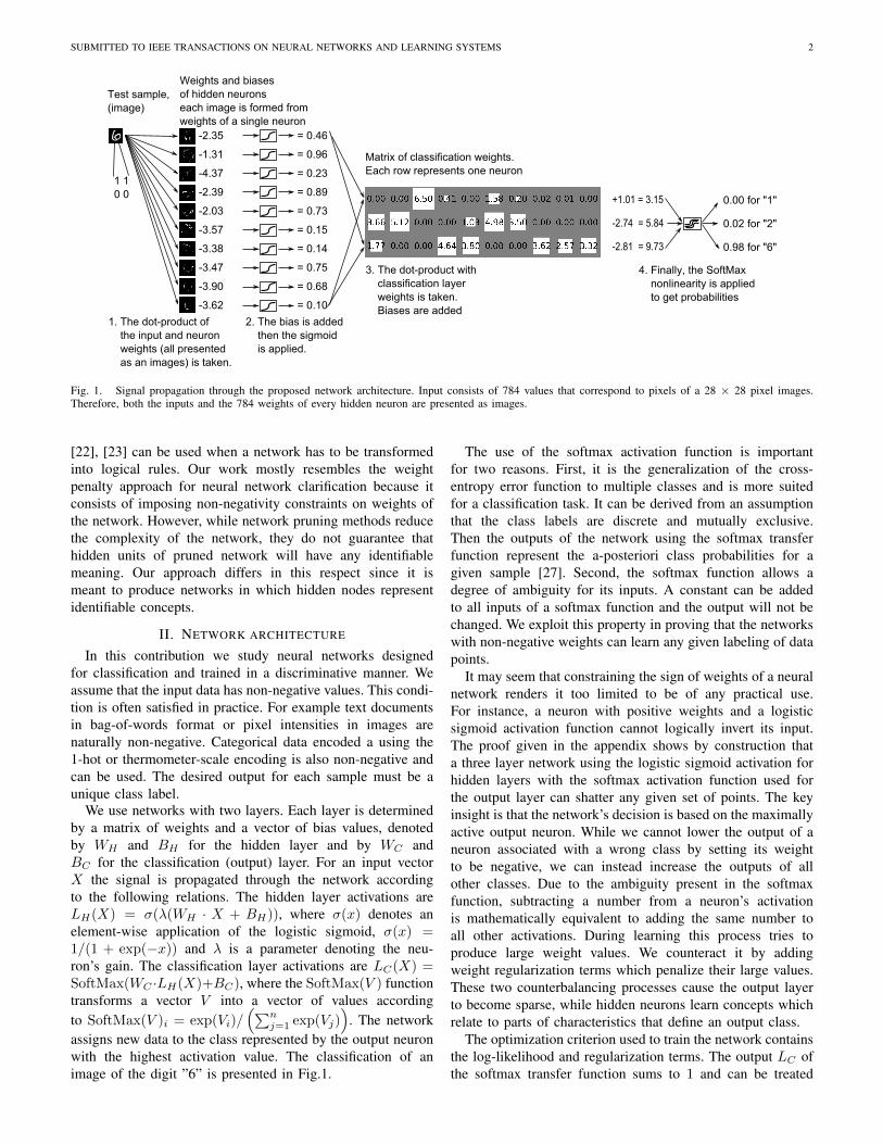
Fig. 1. Signal propagation through the proposed network architecture. Input consists of 784 values that correspond to pixels of a 28 × 28 pixel images.Therefore, both the inputs and the 784 weights of every hidden neuron are presented as images.

[22], [23] can be used when a network has to be transformedinto logical rules. Our work mostly resembles the weightpenalty approach for neural network clarification because itconsists of imposing non-negativity constraints on weights ofthe network. However, while network pruning methods reducethe complexity of the network, they do not guarantee thathidden units of pruned network will have any identifiablemeaning. Our approach differs in this respect since it ismeant to produce networks in which hidden nodes representidentifiable concepts.

II. NETWORK ARCHITECTURE

In this contribution we study neural networks designedfor classification and trained in a discriminative manner. Weassume that the input data has non-negative values. This condi-tion is often satisfied in practice. For example text documentsin bag-of-words format or pixel intensities in images arenaturally non-negative. Categorical data encoded a using the1-hot or thermometer-scale encoding is also non-negative andcan be used. The desired output for each sample must be aunique class label.

We use networks with two layers. Each layer is determinedby a matrix of weights and a vector of bias values, denotedby WH and BH for the hidden layer and by WC andBC for the classification (output) layer. For an input vectorX the signal is propagated through the network accordingto the following relations. The hidden layer activations areLH(X) = σ(λ(WH · X + BH)), where σ(x) denotes anelement-wise application of the logistic sigmoid, σ(x) =1/(1 + exp(−x)) and λ is a parameter denoting the neu-ron’s gain. The classification layer activations are LC(X) =SoftMax(WC ·LH(X)+BC), where the SoftMax(V ) functiontransforms a vector V into a vector of values accordingto SoftMax(V )i = exp(Vi)/

(∑nj=1 exp(Vj)

). The network

assigns new data to the class represented by the output neuronwith the highest activation value. The classification of animage of the digit ”6” is presented in Fig.1.

The use of the softmax activation function is importantfor two reasons. First, it is the generalization of the cross-entropy error function to multiple classes and is more suitedfor a classification task. It can be derived from an assumptionthat the class labels are discrete and mutually exclusive.Then the outputs of the network using the softmax transferfunction represent the a-posteriori class probabilities for agiven sample [27]. Second, the softmax function allows adegree of ambiguity for its inputs. A constant can be addedto all inputs of a softmax function and the output will not bechanged. We exploit this property in proving that the networkswith non-negative weights can learn any given labeling of datapoints.

It may seem that constraining the sign of weights of a neuralnetwork renders it too limited to be of any practical use.For instance, a neuron with positive weights and a logisticsigmoid activation function cannot logically invert its input.The proof given in the appendix shows by construction thata three layer network using the logistic sigmoid activation forhidden layers with the softmax activation function used forthe output layer can shatter any given set of points. The keyinsight is that the network’s decision is based on the maximallyactive output neuron. While we cannot lower the output of aneuron associated with a wrong class by setting its weightto be negative, we can instead increase the outputs of allother classes. Due to the ambiguity present in the softmaxfunction, subtracting a number from a neuron’s activationis mathematically equivalent to adding the same number toall other activations. During learning this process tries toproduce large weight values. We counteract it by addingweight regularization terms which penalize their large values.These two counterbalancing processes cause the output layerto become sparse, while hidden neurons learn concepts whichrelate to parts of characteristics that define an output class.

The optimization criterion used to train the network containsthe log-likelihood and regularization terms. The output LC ofthe softmax transfer function sums to 1 and can be treated


as the a-posteriori probabilities of class labels given theinput. We follow this interpretation and train the networkby minimizing the negative log-likelihood of observing thegiven data set. Furthermore, the weights are regularized byminimizing their absolute values (`1 norm) and their squares(`2 norm) [18], [19], thus we employ a penalty-based weightpruning mechanism. The combined action of the `1 and`2 penalties both selects important connections and limitstheir magnitude. Sparse activations of the hidden layer canadditionally be enforced by minimizing the sum of the hiddenneuron activations. This further enhances readability – properclassification of a sample must depend on only a few hiddenneurons becoming active. The complete optimization target is:

Loss =− 1

n

n∑S=1

log(LC(X

S)YS

)+∑i,j

(pH1 |WH i,j |+ pH2W

2H i,j

)+∑j,k

(pC1 |WC j,k|+ pC2W

2C j,k

)+pSn

n∑S=1

∑j

LH(XS)j

(1)

where n is the number of samples, (XS , Y S) are individualdata samples and pH1, pH2, pC1, pC2, pS are regularizationconstants. The first term of the optimization target is the cross-entropy error, the next two terms regularize the weights, whilethe last term promotes the sparsity of hidden layer activations.We constrain the weight matrices WH and WC to contain onlynon-negative elements. The bias values are unconstrained andoften negative.

Error backpropagation training with gradient descent of anetwork with the logistic sigmoid transfer function, that weuse to keep all the signals non-negative, is numerically difficult[28]. Because the addition of weight constraints makes theoptimization problem even harder, we have chosen to use theL-BFGS-B second-order minimization algorithm [29]. Whenthe training set was too large to be processed as a singlebatch, we have divided it into smaller subsets used for eachepoch. The network was in those cases trained by executinga prescribed number of iterations during which the data werefirst randomly divided into batches of a few thousand samples,then a small number of steps of the L-BFGS-B algorithm wasmade on each batch to minimize (1). Stratified sampling wasused to divide the data into batches to ensure that class labelproportions are retained.

III. EXPERIMENTS

The proposed approach needs the specification of the net-work’s architecture and of five parameters which control theregularization and the steepness of the sigmoid, λ. The numberof hidden neurons was chosen to yield good classificationaccuracy while keeping the network reasonably small. Forthe reduced MNIST and Reuters data the networks have10 and 15 hidden neurons, respectively, which allows easyinspection. For the full MNIST data the number of hiddenneurons had to be increased to 150, which hinders network

TABLE IVALUES OF REGULARIZATION PARAMETERS USED IN THE EXPERIMENTS.

Red. MNIST Full MNIST ReutersNo. hidden 10 10 150 150 15 15No. output 3 3 10 10 10 10Non-neg? F T F T F T

λ Annealed exponentially from 1.0 to 2.0pH1 1e-4 3e-4 0 1e-5 1e-4 1e-4pH2 0 0 0 0 0 0pC1 0 0 0 1e-4 3e-4 3e-4pC2 1e-4 1e-4 1e-4 3e-6 3e-4 3e-4pS 0 0 0 1e-3 0 0

interpretability. However, the hidden weights can be easilyinspected visually when they are presented as images. Formaximum interpretability, the hidden neurons should resemblethreshold gates with only two states: “on” and “off.” Inreality, their output is squashed by the logistic sigmoid intothe range (0, 1). To force the output of hidden neurons tobe close to the limits of this range, the parameter λ wasin all cases gradually increased. To determine the value ofother parameters, we have first trained the network withoutregularization. We have then tested a few values of each ofthe regularization parameters that gave a similar value of thelog-likelihood and regularization terms in (1). In the Table Iwe give the values used for the experiments. We note thatthe imposition of weight non-negativity does not interferewith standard methods of choosing a proper network size andtraining parameters, the reader is referred to textbooks forfurther references on this important topic [4].

In the first experiment we compared networks constructedwith and without non-negativity weight constraints on a subsetof the MNIST handwritten digit data limited to digits 1, 2,and 6. The full MNIST data set contains 60000 training and10000 testing grayscale images of handwritten digits whichwere scaled and centred inside a 28x28 pixel box. It canbe obtained along with a summary of classifiers’ accuraciesfrom http://yann.lecun.com/exdb/mnist/index.html. In this ex-periment small networks with 10 hidden neurons were used.We present a selection of test patterns and the weights of thetwo networks in Fig. 2. An immediate consequence of thenon-negativity constraints is sparsification of weights in theclassification layer. Furthermore, the patterns learned by thehidden neurons allow easy interpretation. They are localizedand tend to look like parts of digits (e.g. the images of weightsof neurons in the columns 2-4 of the fourth row of Fig. 2 looklike the rounded bottom of digit 6). In contrast, the hiddenneurons of the unconstrained network are less localized. Theycontain both positive and negative weights covering most ofthe input image, which makes it harder to visualize to whatpatterns they respond. The bar charts indicate the activationsof hidden neurons for the sample input patterns. It can be seenthat neurons in both networks discriminate between digits andtend to work in the nonlinear parts of their activation functions,resembling threshold gates. The unconstrained network ismore accurate and achieves 1% error rate, compared with 1.5%for the constrained one. In general, the trend was observedthat more understandable networks show lower accuracy. Webelieve that in certain situations a better insight into the data


(a)

(b)

(c)

Fig. 2. (a) Exemplary digits from the MNIST dataset. The weights of anetwork trained (b) without constraints and (c) with non-negative constraints.The weights of the classification (output) layer are plotted as a diagram withone row for each output neuron and one column for every hidden (input)neuron. The area of each square is proportional to the weight’s magnitude;white indicates positive and black negative sign. Below each column of thediagram, the weights of hidden neurons are printed as an image. The intensityof each pixel is proportional to the magnitude of the weight connected to thatpixel in the input image with, the value 0 corresponding to gray in (b) andto black in (c). The biases are not shown. The hidden neurons have beenrearranged for better presentation. The bar charts at the bottom of the plotsshow the activation of hidden neurons for the digits presented in (a). Each rowdepicts the activations of each hidden neuron for five color-coded examplesof the same digit.

outweighs the benefits of an accurate but opaque classifier.In the next large-scale experiment, we used the full MNIST

data to build a constrained and unconstrained neural networkwith 150 hidden neurons and 10 outputs. We compare inFig. 3 the depictions of weights of 32 randomly selectedhidden neurons with 32 features obtained with PCA andwith 32 obtained with NMF. Full networks are shown in

the Fig.6 and 7 in the appendix. The unconstrained networkshows a much lower error rate of 2.4%, compared with4.9% for the constrained one. To put those numbers intoperspective, state-of-the-art 1998 error rate on the MNIST fora two layer neural network was 4.7%. Once again, the non-negativity constraints result in the emergence of sparser andmore localized weight distributions of the hidden neurons,which often filter distinctive parts of digits. In contrast, thehidden neurons of the unconstrained network react to wholepictures, thus it is difficult to estimate intuitively their influenceon the classifier’s output. Similarly, the patterns learned byPCA are holistic, non-localized ones. But for the first few, itis hard to describe their contents. It is also difficult to seehow they relate to the shapes of different digits. Further, theNMF has learned sparse, localized, and interpretable features.However, only a few patterns resemble parts of digits, likethe vertical bar (shown in the last column of Fig. 7). Mostof the features seem to down-sample input images on a non-uniform grid and do not provide cues for classification. Thisis caused by two factors. First, unlike the neural network withnon-negative constraints on weights, the NMF model does notaim at class discrimination. Second, NMF imposes no limitson the number of features activated by a sample. Increasingthe rank of factorization (the total number of features) onlyworsens the issue, as in the limit the identity matrix is atrivial NMF factor. In this case each NMF feature will be asingle pixel and the NMF-transformed data will not be moreuseful for data analysis. On the other hand, decreasing therank leads the NMF features to look like blurred shapes ofthe simplest digits. The addition of a constraint on the numberof coactive features, while allowing a large total number offeatures, has been shown to promote the learning of a parts-based decomposition [30]–[32]. This is because, in contrast toa limited-rank decomposition, we assume a large dictionary offeatures which, in turn, must be complex enough to provideadequate input reconstruction from just the few active ones.

In the last experiment we compared the networks on theReuters-21578 text categorization collection. It is composed ofdocuments that appeared in the Reuters newswire in 1987. Weused the ModApte split limited to ten most frequent categories.We have used a processed (stemming, stop-word removal)version in bag-of-words format obtained from http://people.kyb.tuebingen.mpg.de/pgehler/rap/. This dataset is challengingbecause the borders between topics are fuzzy and documentsmay belong to many categories simultaneously. During train-ing such documents were used with all possible labels. Fortesting a document was counted as correctly classified whenthe network assigned it to one of the classes to which itbelonged. The networks had 15 hidden and 10 output neurons(one for each category). The unconstrained network is slightlymore accurate and achieves an error rate of 12.4%, comparedwith 12.8% for the constrained one. The weights of the twonetworks are portrayed in Fig. 4. We provide an interpretationof the hidden neurons by listing words associated with thestrongest weights. The word “blah” has no meaning and isartificially added noise. The non-negative network has beenobserved to be more sensitive to it, as many hidden neuronsreact to it. The neurons in the unconstrained network seem to


(a) (b)

(c) (d)

Fig. 3. Weights of randomly selected 32 out of 150 hidden neurons ofunconstrained network (a) and network with weigth non-negativity constraints(b). 32 first principal components (c). 32 filters learned by NMF (d).

convey meaning by being both active and inactive, because thewords associated with positive and negative weights fall intodistinct categories. Furthermore, the matrix of output weightsis dense and difficult to interpret. On the other hand, the outputweights of the non-negative network are sparse and allow foran interpretation of relations between topics. The closeness oftopics “corn”, “grain”, and “wheat” is detected as the weightsfor those categories form a cluster. The topic “trade” is linkedto categories describing goods that can be traded. The wordslisted for hidden neurons corroborate those interpretations, e.g.the neuron shown in the ninth row of Fig. 4(b) reacts towords “trade”, “rate”, “fed”, “dollar” is linked through theclassificatoin weights matrix to topics “money-fx” (foreign

(a)

(b)

Fig. 4. Networks trained on the Reuters-21578 data: with unconstrainedweights (a) and with non-negative weight constraints (b). Input neurons arecharacterized by listing ten words connected to weights having large absolutevalue. The + and - signs indicate the sign of the weight in (a). Each column ofthe diagram depicts weights of an output neuron, the size varies with weightvalue and black or white filling indicates sign as in Fig. 2. The neurons havebeen rearranged for better presentation.

exchange), “interest”, and “trade”.

A. Experiment running times

We have compared the time necessary to train networks withand without the non-negativity constraints. The constrainednetworks required about twice as much epochs (passes throughthe full training set) to converge. However, a single epochtook only slightly more time for the constrained networks.This may be due to the fact that we have used the same L-BFGS-B implementation for both cases, imposing improperconstraints (−∞,∞) for the unconstrained networks. On thelargest dataset considered, the full MNIST benchmark, theunconstrained network required 3 epochs which took 15minutes on our machine. In contrast, the network with non-negative weights required 6 epochs which took 37 minutes.Even though the constrained networks require more trainingtime, we believe that a slowdown of 2-3 times compared withthe unconstrained networks is acceptable in practice.

IV. CONCLUSION

We have demonstrated how constraining the weights ofa neural network to be non-negative improves network un-derstandability and leads to intuitively understandable hiddenneurons. To the best of our knowledge, this is the first attemptat discriminative training of understandable neural networkson large, nontrivial datasets.

Deriving understandable descriptions of observations is thehallmark of human intelligence. Our approach is but a singlestep on the road towards pattern recognition tools that help not


only to make predictions about data, but also empower theiruser with new insights and concepts derived from that data.

APPENDIX APROOF OF THE SHATTERING PROPERTY OF NETWORKS

WITH NON-NEGATIVE WEIGHTS

We will show that a three layer network can shatter everycombination of points. First, we show that adding a constantto all output weights doesn’t change the value of the softmaxfunction. Let the output layer compute the function:

LC = SoftMax(W · LH +B), (2)

where LC is the vector of classification (output) layer activa-tions, W is the weight matrix, LH is the vector of hidden layeractivations, and B is the vector of bias values. Let 1 denotematrix whose all elements are 1 and let a be a constant. Then:

SoftMax ((a1+W )LH +B) =

SoftMax(a1 · LH +W · LH +B).(3)

For simplicity, substitute C =W ·LH+B. The product 1·LH

is a vector whose all elements are equal to the sum of LH . Itfollows that:

SoftMax(a1LH + C)i =exp (

∑LH) exp(Ci)∑n

j=1 exp (∑LH) exp(Cj)

= SoftMax(C)i

(4)

Hence we can transform any network with negative weightsin the output layer into one with only non-negative weightsby adding a large enough constant.

We will construct a three layer (2 hidden layers withsigmoid activation function followed by a classification layerwith softmax activation) that will shatter a given set of mpoints described by their position in a n-dimensional space.Let X ∈ Rn×m be the data matrix. We will show how toconstruct a network returning any labeling of those points.For simplicity we will assume that the gains in the logisticsigmoid transfer functions are infinite and the hidden neuronsactivations are always 0 or 1.

There are O(nm) neurons in the first hidden layer. Forevery input dimension we first project all data points ontothis dimension, then we select at most m threshold valuesbetween the projections. We add hidden neurons with a singlenonzero weight equal to 1 corresponding to this dimensionand bias equal to the threshold. Unless two columns of X arethe same (i.e. two points are at exactly the same position),the activations H1 of the first hidden layer are unique binaryvectors. An two-dimensional example is shown in Fig.5. Twothreshold values are selected for each dimension. Each of thethresholds corresponds to a cut through the data plane andis implemented a single neuron. The weights of neurons aregiven – they are binary and uniquely identify each point.

There are m neurons in the second hidden layer, onefor each point. Their weights are equal, the weight Wi,j

connecting the j-th neuron in the first hidden layer to the i-thneuron in the second one equals to 2j. Thus if we treat thefirst hidden layer activations as binary numbers, the productsW ·H1 are their decimal values. To every point corresponds

P1

P3

P4 P2

N3 N4

N2

N1

P1 P2 P3 P4 P5

N1 1 0 1 0 1

N2 1 0 0 0 1

N3 0 0 1 1 1

N4 0 0 0 1 1

P5

Fig. 5. Construction of a network with non-negative weights.

one such number and we can order the points accordingto them. If the second hidden layer bias values are set tovalues in-between those numbers, the activations of the secondhidden layer create a full-rank binary matrix (if the points arereordered, then for the k-th point the k first neurons are active,while the m−k remaining ones are zero. Hence the activationmatrix is triangular.) Thus we can solve for output weights forevery possible labeling of data points. In the last step we add aconstant to output weights to ensure that all are non-negative.

APPENDIX BFULL PICTURES OF NETWORKS TRAINED ON MNIST DATA

ACKNOWLEDGMENT

The authors would like to thank the anonymous reviewersfor their many insightful comments and a careful proofing ofthis manuscript.

REFERENCES

[1] L. Breiman, J. H. Friedman, R. A. Olshen, and C. J. Stone, Classificationand Regression Trees, ser. Statistics/Probability Series, C. Hall Crc, Ed.Wadsworth, 1984, vol. 19, no. Book, Whole.

[2] J. R. Quinlan, C4.5: Programs for Machine Learning, M. B. Morgan,C. Leyba, and J. Hammett, Eds. Morgan Kaufmann, 1992.

[3] W. W. Cohen, “Fast effective rule induction,” in Proc. 12th Int. Conf.Mach. Learning (ICML), 1995.

[4] J. M. Zurada, Introduction to artificial neural systems. West PublishingCompany, 1992.

[5] R. Andrews, J. Diederich, and A. B. Tickle, “Survey and critique oftechniques for extracting rules from trained artificial neural networks,”Knowledge-Based Systems, vol. 8, no. 6, pp. 373–389, Dec. 1995.

[6] W. Duch, R. Setiono, and J. Zurada, “Computational intelligence meth-ods for rule-based data understanding,” Proceedings of the IEEE, vol. 92,no. 5, pp. 771–805, May 2004.

[7] B. Baesens, R. Setiono, C. Mues, and J. Vanthienen, “Using Neural Net-work Rule Extraction and Decision Tables for Credit-Risk Evaluation,”Management Science, vol. 49, no. 3, pp. 312–329, Mar. 2003.

[8] D. D. Lee and H. S. Seung, “Learning the parts of objects by non-negative matrix factorization.” Nature, vol. 401, no. 6755, pp. 788–91,Oct. 1999.

[9] P. Paatero, “Least squares formulation of robust non-negative factoranalysis,” Chemometrics and Intelligent Laboratory Systems, vol. 37,no. 1, pp. 23–35, May 1997.

[10] A. J. Bell and T. J. Sejnowski, “The "independent components" ofnatural scenes are edge filters,” Vision research, vol. 37, no. 23, pp.3327–38, Dec. 1997.

[11] D. T. Jones, “Protein secondary structure prediction based on position-specific scoring matrices.” Journal of molecular biology, vol. 292, no. 2,pp. 195–202, Sep. 1999.

[12] G. E. Hinton and R. R. Salakhutdinov, “Reducing the dimensionality ofdata with neural networks.” Science, vol. 313, no. 5786, pp. 504–7, Jul.2006.

[13] Y. Bengio, “Learning Deep Architectures for AI,” Foundations andTrends in Machine Learning, vol. 2, no. 1, pp. 1–127, 2009.

[14] R. Reed, “Pruning algorithms-a survey,” Neural Networks, IEEE Trans-actions on, vol. 4, no. 5, pp. 740–747, 1993.


Fig. 6. The weights of a network trained on the full MNIST dataset without weight constraints. The weights of the classification (output) layer are plottedas a diagram with one row for each output neuron and one column for every hidden (input) neuron. The area of each square is proportional to the weight’smagnitude; white indicates positive and black negative sign. Below each column of the diagram, the weights of hidden neurons are printed as an image. Theintensity of each pixel is proportional to the magnitude of the weight connected to that pixel in the input image with, the value 0 corresponding to gray. Thebiases are not shown. The hidden neurons have been rearranged for better presentation.


Fig. 7. The weights of a network trained on the full MNIST dataset with non-negativity weight constraints. The weights of the classification (output) layerare plotted as a diagram with one row for each output neuron and one column for every hidden (input) neuron. The area of each square is proportional to theweight’s magnitude. Below each column of the diagram, the weights of hidden neurons are printed as an image. The intensity of each pixel is proportionalto the magnitude of the weight connected to that pixel in the input image with, the value 0 corresponding to black. The biases are not shown. The hiddenneurons have been rearranged for better presentation.


[15] Y. Le Cun, J. Denker, S. Solla, R. Howard, and L. Jackel, “Optimal braindamage,” Advances in neural information processing systems, vol. 2,1990.

[16] B. Hassibi, D. Stork, and G. Wolff, “Optimal brain surgeon and gen-eral network pruning,” in Neural Networks, 1993., IEEE InternationalConference on. IEEE, 1993, pp. 293–299.

[17] G. Castellano, A. Fanelli, and M. Pelillo, “An iterative pruning algorithmfor feedforward neural networks,” Neural Networks, IEEE Transactionson, vol. 8, no. 3, pp. 519–31, Jan. 1997.

[18] M. Ishikawa, “Structural learning with forgetting,” Neural Networks,vol. 9, no. 3, pp. 509–521, Apr. 1996.

[19] H. Zou and T. Hastie, “Regularization and variable selection via theelastic net,” Journal of the Royal Statistical Society: Series B (StatisticalMethodology), vol. 67, no. 2, pp. 301–320, Apr. 2005.

[20] S. Nowlan and G. Hinton, “Simplifying neural networks by soft weight-sharing,” Neural computation, vol. 4, no. 4, pp. 473–493, 1992.

[21] R. Setiono, “Extracting M-of-N rules from trained neural networks,”Neural Networks, IEEE Transactions on, vol. 11, no. 2, pp. 512–519,2000.

[22] T. Huynh and J. Reggia, “Guiding hidden layer representations forimproved rule extraction from neural networks,” Neural Networks, IEEETransactions on, vol. 22, no. 2, pp. 264–75, Feb. 2011.

[23] J. Chorowski and J. M. Zurada, “Extracting Rules from Neural Networksas Decision Diagrams,” Neural Networks, IEEE Transactions on, vol. 22,no. 12, pp. 2435–46, Dec. 2011.

[24] P. Bartlett, “The sample complexity of pattern classification with neuralnetworks: the size of the weights is more important than the size of thenetwork,” IEEE Transactions on Information Theory, vol. 44, no. 2, pp.525–536, 1998.

[25] A. Krogh and J. A. Hertz, “A simple weight decay can improvegeneralization,” in Advances in neural information and processingsystems, 1991. [Online]. Available: http://books.nips.cc/papers/files/nips04/0950.pdf

[26] G. Gnecco and M. Sanguineti, “Regularization techniques andsuboptimal solutions to optimization problems in learning from data,”Neural Computation, vol. 22, no. 3, pp. 793–829, Nov. 2009. [Online].Available: http://dx.doi.org/10.1162/neco.2009.05-08-786

[27] C. M. Bishop, Neural Networks for Pattern Recognition. New York,NY, USA: Oxford University Press, Inc., 1995.

[28] Y. LeCun, L. Bottou, G. Orr, and K. Müller, “Efficient backprop,” Neuralnetworks: Tricks of the trade, vol. 1524, no. 3, 1998.

[29] C. Zhu, R. H. Byrd, P. Lu, and J. Nocedal, “Algorithm 778: L-BFGS-B: Fortran subroutines for large-scale bound-constrained optimization,”ACM Transactions on Mathematical Software, vol. 23, no. 4, pp. 550–560, Dec. 1997.

[30] B. Olshausen and D. Field, “Sparse coding with an overcomplete basisset: A strategy employed by V1?” Vision research, vol. 37, no. 23, pp.3311–3325, 1997.

[31] P. O. Hoyer, “Non-negative matrix factorization with sparseness con-straints,” Journal of Machine Learning Research, vol. 5, pp. 1457–1469,Aug. 2004.

[32] M. Y. Ranzato, L. Boureau, and Y. LeCun, “Sparse feature learning fordeep belief networks,” in Advances in neural information processingsystems, 2007.

Jan Chorowski received the MSc degree in elec-trical engineering from the Wrocław University ofTechnology, Poland and the PhD degree from theUniversity of Louisville, Kentucky where he was therecipient of the University Scholarship. His researchinterests include the development of machine learn-ing algorithms, especially using neural networks.

Jacek M. Zurada received the MS and PhD degrees(with distinction) in electrical engineering from theTechnical University of Gdansk, Poland, in 1968 and1975, respectively. Since 1989, he has been a pro-fessor in the Department of Electrical and ComputerEngineering, University of Louisville, Kentucky. Hewas the department chair from 2004 to 2006. Hewas an associate editor of the IEEE Transactionson Circuits and Systems, Part I and Part II, andserved on the editorial board of the Proceedingsof IEEE. From 1998 to 2003, he was the editor-

in-chief of the IEEE Transactions on Neural Networks. He is an associateeditor of Neural Networks, Neurocomputing, Schedae Informaticae, and theInternational Journal of Applied Mathematics and Computer Science, theadvisory editor of the International Journal of Information Technology andIntelligent Computing, and the editor of Springer’s Natural Computing BookSeries. He has served the profession and the IEEE in various elected capacities,including as the President of the IEEE Computational Intelligence Society in2004-2005. In 2013he serves as IEEE Technical Activities Chair-Elect andChair the IEEE TAB Periodicals Review and Advisory Committee. He is aDistinguished Speaker of IEEE CIS and a Fellow of the IEEE.

submitted to ieee transactions on neural networks...

Documents