subjective well-being: keeping up with the perception of...
TRANSCRIPT

Subjective well-being: Keeping up with the perception
of the Joneses.
Cahit Guven ∗
Deakin University
Bent E. Sørensen †
University of Houston and CEPR
July 2011
Abstract
Using data from the U.S. General Social Survey 1972-2004, we study the role ofperceptions and status in self-reported happiness. Reference group income negativelyrelates to own happiness and high perceptions about own relative income, quality ofdwelling, and social class relate positively and very significantly to happiness. Percep-tions about income and status matter more for females, and for low income, conser-vative, more social, and less trusting individuals. Dwelling perceptions matter morefor males, and for middle income, married, conservative, more social, and less trustingindividuals.
FIGURES: 3TABLES: 10WORDS:9597
JEL Classification: D14, D63, I31,Keywords: happiness, social comparison, status, perceptions.
∗Deakin University, Melbourne, Victoria, Australia†Department of Economics, University of Houston, TX, 77204, e-mail: [email protected], tel:
713 7433841, fax: 713 7433798. The authors thank several referees and participants at the InternationalConference on Policies for Happiness in Sienna, the 76th Annual SEA Meetings, the 11th Texas EconometricsCamp, the 7th Annual Missouri Economics Conference, and seminar participants at Sam Houston StateUniversity and the University of Houston for their valuable comments and suggestions. Special thanks toRainer Winkelmann.

1 Introduction
“Happiness is not achieved by the conscious pursuit of happiness; it is generally the by-
product of other activities.” Aldous Leonard Huxley (July 26, 1894 - November 22, 1963)
British philosopher.
We study self-reported happiness which we also refer to as “subjective well-being” using
data from the U.S. General Social Survey (GSS) 1972-2004 which has surveyed about 3000
individuals annually or biennially since 1970.1 The GSS provides self-reported measures of
well-being; i.e., responses to questions about how happy individual respondents are with
their lives.
The economics profession has been wary of attempts to use measures of happiness in spite
of the ubiquitous use of utility functions. We follow the convention of reserving the term “util-
ity” for describing individuals’ choices between economic variables; however, self-reported
well-being is related to “utility” in the sense that well-being helps predict individuals’ eco-
nomic choices; see the survey by Frey and Stutzer (2002). Higher income allows people to
purchase more goods which is expected to increase well-being but people also derive happi-
ness from high relative income. Luttmer (2005) shows that well-being depends on relative
consumption in addition to absolute consumption in the United States. He uses income as a
proxy for consumption and finds that neighbors’ income has a significant negative influence
on individual well-being. In addition, Clark and Oswald (1996) find that workers’ reported
satisfaction is inversely related to their comparison wage rates. However, Clark et al. (2009)
find a positive relationship between neighborhood income and happiness, consistent with
findings in Senik (2009). Clark and Senik (2010) find that, in Europe, colleagues are the
most frequently-cited reference group for income comparisons.
We find that income relative to individuals’ own cohort working in the same occupation
group and living in the same region matters for happiness.2 We then investigate the unex-
plored issue of whether or not the perception of relative income matters in addition to actual
1The GSS is in transition from a replication cross-sectional design to a design that uses rotating panels.In 2008 there were two components: a new 2008 cross-section with 2,023 cases and the first re-interviewswith 1,536 respondents from the 2006 GSS, however these data are not available yet but will be available inthe future.
2We tried different reference groups such as people living in the same region. To save space, we do notreport these results. See Senik (2009) and Rablen (2008) for more discussion on income comparisons andthe choice of reference groups.
1

relative income. We do not have exogenous shifters of perceptions so terms like “matters”
should not be understand in a causal sense but only as a predictive correlation. In the GSS,
unlike most other surveys, individuals are asked their opinion about their income relative
to an average American family and their opinion about what social class they belong to.
We show that perceptions about relative income are highly correlated with happiness. After
controlling for own income and reference group income, higher perceptions about relative
income predict higher happiness. If people care about their relative standing in the soci-
ety, social class may be important and, indeed, we find that perceived social class is highly
positively correlated with happiness while actual social class is of little importance.
We consider perceived dwelling status as a predictor of happiness and find that per-
ceptions about own dwelling, relative to others in the city and neighborhood, matter for
happiness, even after controlling for dwelling ownership, dwelling type, and various neigh-
borhood characteristics. Perceived dwelling status relative to others in the neighborhood is
more important than perceptions about dwellings in the broader city. Because people typi-
cally observe neighborhood residences more than other residences in the city, this strengthens
the conclusion that relative, rather than absolute, status matters.
Perceptions about relative income are more important for individuals who still live in the
city in which they grew up (“non-movers”), females, and conservatives as well as low income
individuals while perceived social class matters more for and conservatives. Perceptions
about one’s dwelling are more important in explaining happiness for non-movers, males, and
conservatives. Inequality aversion lessens the influence of income and social class perceptions
but strengthens the impact of dwelling perceptions. The results are robust to selection,
different sub-samples, selection of reference group, controlling for income and happiness
shocks, and estimation techniques.
Section 2 gives an overview of the literature on happiness and Section 3 discusses the
data and the construction of the variables used in the paper. Section 4 presents the basic
framework and the estimation strategy while Section 5 presents descriptive statistics. Sec-
tion 6 presents the empirical results of the paper and Section 7 concludes. The Appendix
gives more detailed information about the GSS and the variables used. In the Appendix, we
also display and discuss the results from a battery of robustness regressions.
2

2 Related literature
Oswald (1997) shows that happiness with life is rising in the United States but the increase
is small—it seems that extra income is not contributing much to the quality of peoples’ lives.
Since the early 1970s, reported levels of satisfaction with life in European countries have,
on average, risen very slightly and other scholars have found that the proportion of people
considering themselves to be “very happy” has fallen over the same time period, in spite
of increasing income levels. Recently, Graham (2004) argues that absolute income matters
up to a certain point—particularly when basic needs are not met—but after that, relative
income matters more.
Adaptation and social comparison are possible explanations why increases in absolute
income are not reflected in happiness. In a recent study, Di Tella et al. (2010) find strong
adaptation to changes in income in Germany but not to changes in status. In sub-samples,
they find no adaptation to income for males, right-wingers, and self-employed but females,
left-wingers, and employees show adaptation to income. However, the latter group do not
show adaptation to status.
Many economists have noted that individuals compare themselves to others with respect
to income, consumption, status, or utility. In other words, relative income may matter more
than actual income; see the survey by Clark et al. (2008). Van Praag and Kapteyn (1973)
construct an econometrically estimated welfare function with a “preference shift” parameter
that captures the tendency of material wants to increase as income increases. They find that
increases in income shift aspirations upward and this preference shift destroys about 60 to
80 percent of the welfare effect of an increase in income.
High income aspirations may also be formed during childhood. Winkelmann et al. (2007c)
find a negative externality of parental income on children’s current well-being with children
comparing their actual income with the acquired aspiration level. There are a number of
reasons why an interpretation based chiefly on “relativity” notions is plausible. A certain
amount of empirical support has been developed for the relative income concept in other
economic applications, such as savings behavior and, more recently, fertility behavior and la-
bor force participation (Duesenberry, 1949; Easterlin, 1963, 1973; Freedman, 1963; Wachter,
1972, 1974).
Economists have identified a U-shaped relationship between age and happiness (Oswald
3

1997, Blanchflower and Oswald, 2000). For several reasons, it is difficult to capture the
influence of age on well-being. The term happiness may change its meaning with age and
the age effect may interfere with a cohort effect. The direction of causation is also unclear
because happy people tend to live longer which contributes to a positive correlation between
age and happiness. Happiness and health are highly correlated and Wright (1985) finds an
effect of self-rated health on satisfaction which is not affected by comparison with others.
Blacks tend to be less happy than whites in all psychological and sociological studies in
the United States. This also holds for other countries such as South Africa, where whites
are happiest followed by Indians, coloreds, and blacks (Moller, 1989). A major reason for
lower subjective well-being of blacks may be lower self-esteem, which in turn may be caused
by lower status in society. Economists have also found that American blacks are less happy
than whites (Blanchflower and Oswald, 2000).
The level of education bears little relationship to happiness. Education may indirectly
contribute to happiness by allowing for a better adaptation to changing environments but it
also tends to raise aspiration levels. It has, for instance, been found that highly educated are
more distressed than less educated when hit by unemployment (Clark and Oswald, 1994).
3 Data
We use GSS data from 1972 to 2004. The GSS consists of cross-sectional surveys conducted
by the National Opinion Research Center (NORC) in the United States annually 1972-1994,
except for the years 1979, 1981, and 1992, and biennially beginning in 1994. The main areas
covered in the GSS include socioeconomic status, social mobility, social control, family,
race relations, sexual relations, civil liberties, and morality. Our dependent variable is the
response to the question, “Taken all together, how would you say things are these days—
would you say that you are very happy, pretty happy, or not too happy?” The response is
recoded as a categorical variable taking the values 1, 2, and 3 which in order refers to “not
too happy,” “pretty happy,” and “very happy.” (The answers “don’t know,” “no answer,”
and “not applicable” are recorded as missing.) As shown in Figure 1, there is substantial
variation in respondents’ happiness levels. 32 percent of the respondents are “very happy,”
56 percent are “pretty happy,” while 12 percent are “not too happy.”
In the GSS, income is a categorical variable taking values 1–13 where 13 is the highest
4

income level. In order to calculate relative income, we use the midpoint method.3 The lowest
and the highest income values in a category are known and we calculate each household’s
income as the midpoint income of that category, normalized by the Consumer Price Index
(CPI). In the regressions, we use actual income as a continuous variable but because perceived
relative income is a categorical variable with 5 categories, we also recode actual income into
5 categories in order to make it comparable.
Reference group income is the average income of a reference group. We tried reference
groups with different ranges for age, region, and occupational sector (one and three digit
sectors and occupations) and chose the group which provides the best fit in the regressions.
The reference group used in the regressions is the individuals’ own cohort working in the
same occupation group (one digit) and living in the same region. In the regressions, we use
reference group income as a continuous variable but we also recode reference group income
into 5 categories. People know their own current actual income but they may not have
current information about others’ current income. In this case, reference group income may
be the lagged average reference group income. We therefore attempte to use the income of
the reference group in the previous period as well.
Perceived relative income is the answer to the question, “Compared with American fami-
lies in general, would you say your family income is far below average, below average, average,
above average, or far above average?” This variable has 5 categories: “far below average,”
“below average,” “average,” “above average,” and “far above average.” (“Don’t know,” “no
answer,” and “not applicable” are recorded as missing.) In the regressions, we use perceived
relative income as a categorical variable but since actual relative income is a continuous
variable, we also use perceived relative income as a continuous variable taking values from 1
through 5. There is substantial variation in perceived relative income as shown in Figure 1.
5 percent of the sample are “far below average,” 24 percent “below average,” 51 percent
“average,” 19 percent “above average,” and 2 percent “far above average.”
Perceived social class is the answer to the question, “If you were asked to use one of
four names for your social class, which would you say you belong in: the lower class, the
working class, the middle class, or the upper class?” This variable has 4 categories: “lower
class,” “working class,” “middle class,” and “upper class.” (The answers “don’t know,” “no
3GSS also created its own household income variable which is available in the dataset and we checked ourresults with this variable as well.
5

answer,” and “not applicable” are recorded as missing .) In the regressions, we use perceived
social status as a categorical variable but since occupational prestige and socio-economic
index are used as the control variables and are continuous variables, we also use perceived
social status as a continuous variable taking values from 1 through 4 to make it comparable.
As shown in Figure 1, 5 percent of the sample are “lower class,” 46 percent “working class,”
46 percent “middle class,” and 3 percent “upper class.”
Perceptions about dwelling relative to other dwellings in the city and the neighborhood
are the answers to the questions 1) “Compared to apartments/houses in the neighborhood,
would you say the house/apartment is far below average, below average, average, above aver-
age, or far above average?” and 2) “Compared to apartments/houses in the city/town/county,
would you say the house was far below average, below average, average, above average, or
far above average?” The answers take values 1-5 which corresponds to “far below average,”
“below average,” “average,” “above average,” and “far above average.” We control for the
type of the dwelling in the regressions which is coded as follows: Trailer (1), detached single
family house (2), 2-family house, 2 units side by side (3), 2-family house, 2 units one above
the other (4), detached 3-4 family house (5), row house (6), apartment house, 3 stories or less
(7), apartment house, 4 stories or more (8), apartment in a partly commercial structure (9),
other (10). We also control for the dwelling ownership which is the answer to the question
“(Do you/does your family) own your (home/apartment), pay rent, or what?” Answers are
coded as follows: “own or is buying,” “pays rent,” and “other.” The distribution of the per-
ceptions about dwellings compared to houses in the city are similar to a normal distribution
as shown in Figure 1 while perceptions relative to neighborhood are more clustered around
the middle value. Around 71 percent of individuals in the sample consider their dwelling
“average” relative to others in the neighborhood but this number is only 57 percent relative
to others in the city.
Socio-Economic Index scores are originally calculated by Otis Dudley Duncan based on
NORC’s North-Hatt prestige study. Duncan regresses prestige scores for 45 occupational
titles on education and income to produce weights that would predict prestige. This algo-
rithm is then used to calculate socio-economic index scores for all occupational categories
employed in the Census classification of occupations. Similar procedures have been used to
produce socio-economic scores based on later NORC prestige studies and censuses.
Regions: New England, Middle Atlantic, East North Central, West North Central, South
6

Atlantic, East South Central, West South Central, Mountain, Pacific, Foreign. Sectors:
Agriculture, Construction, Mining, Manufacturing, Transportation, Retail Trade, Wholesale,
Finance, Entertainment, Public Administration. For further details and the exact definitions
of other variables used, see the Appendix.
4 Empirical Framework
In the empirical analysis, we estimate self-reported happiness of an individual i at time t
as a function of his/her logarithm (ln) reference group income and ln household income
together with the following control variables: dwelling ownership, ln weekly working hours,
labor force status, sex, age, age squared, race, years of education, ln household size, marital
status, religion, ln population of the place of residence, region fixed effects, year fixed effects,
occupation fixed effects, and industry fixed effects. We estimate an OLS model for self-
reported happiness (on a scale 1-3)4 to make the interpretation of the coefficients easy;
however, we report ordered probit estimates in the robustness tables in the Appendix. The
coefficients from the OLS regression are presented with robust standard errors. We use
logarithmic values of the variables in the regressions. However, we also consider levels in
the robustness part, as well as nonlinearities, by recoding main variables into categories.
ln reference group income is the average income of people who live in the same region,
work in the same occupation category (1-digit) and are of the same age as the respondent.
The following equation is our baseline regression and is estimated for the whole sample and
separately for married and nonmarried individuals:
Happinessit = β0 + β1 ln reference group incomeit + β2 ln household incomeit
+controlsit. (1)
We estimate self-reported happiness of an individual i at time t as a function of his/her
ln occupational prestige, ln perceived relative income, ln reference group income, and ln
household income together with the same control variables mentioned above. Perceived
relative income takes the values 1-5 and is treated as a continuous variable while occupa-
tional prestige takes values 0-100 where higher values correspond to higher occupational
4Frijters and Ferrer-i-Carbonell (2003) show that for self-reported happiness, OLS and ordered probitestimates give quite similar results.
7

prestige. Further, we include perceptions about one’s own social class in explaining his/her
happiness—perceived social class takes values 1-4 and is treated as a continuous variable.
We estimate the following equation (including perceived income, prestige, and social class
one-by-one):
Happinessit = β0 + β1 ln reference group incomeit + β2 ln household incomeit
+β3 ln perceived relative incomeit + β4 ln occupational prestigeit
+β5 ln perceived social classit + controlsit. (2)
Next, we consider the role of perceptions about one’s own dwelling compared to other
dwellings in his/her city or neighborhood. We estimate self-reported happiness of an indi-
vidual i at time t as a function of his/her ln perceived dwelling status with respect to other
dwellings in his/her city, type of his/her dwelling as a categorical variable, ln perceived social
class, ln occupational prestige, ln perceived relative income, ln reference group income and
ln household income together with the same control variables mentioned above. Perceived
dwelling status (city) takes values 1-5 and is treated as a continuous variable in the estima-
tion. We use ln values of the variables in the regressions. However, we also consider levels
in the robustness part, as well as nonlinearities, by recoding main variables into categories.
We present the OLS coefficients from the following equation:
Happinessit = β0 + β1 ln reference group incomeit + β2 ln household incomeit
+β3 ln perceived relative incomeit + β4 ln occupational prestigeit
+β5 ln perceived social classit + β7dwelling typeit
+β6 ln perceived dwelling status (city or neighborhood)it + controlsit. (3)
We allow for potential non-monotonicity in our analysis and estimate self-reported hap-
piness of an individual i at time t as a function of his/her perceived dwelling status with
respect to other dwellings in his/her city as a 5 category variable, perceived social class as
a 4 category variable, perceived relative income as a 5 category variable, reference group
income and household income as a 5 category variable which are recoded from the original
data, together with the same control variables mentioned above. We estimate self-reported
8
happiness of an individual i at time t as a function of his/her perceived dwelling status with
respect to other dwellings in his/her city or neighborhood as a 5 category variable as coded
in the codebook, type of his/her dwelling, perceived social class as a 4 category variable
as coded in the codebook, perceived relative income as a 5 category variable as coded in
the codebook, reference group income and household income as a 5 category variable which
are recoded in to 5 categories from the original, together with the same control variables
mentioned above.
The impact of perception may co-vary with gender, income, and other characteristics of
respondents and we examine this issue using interaction effects. We label the variables, such
as gender, as Zit and each of our perception variables as Pit. For each choice of P,Z we
estimate the following equation:
Happinessit = β0 + β1 ln reference group incomeit + β2 ln household incomeit
+β3 ln perceived relative incomeit + β4 ln occupational prestigeit
+β5 ln perceived social classit + β6 ln perceived dwelling status (city)it
+β7 ln perceived dwelling status (neighborhood)it + β8dwelling typeit
+β9Zit + β10Zit ∗Pit + controlsit. (4)
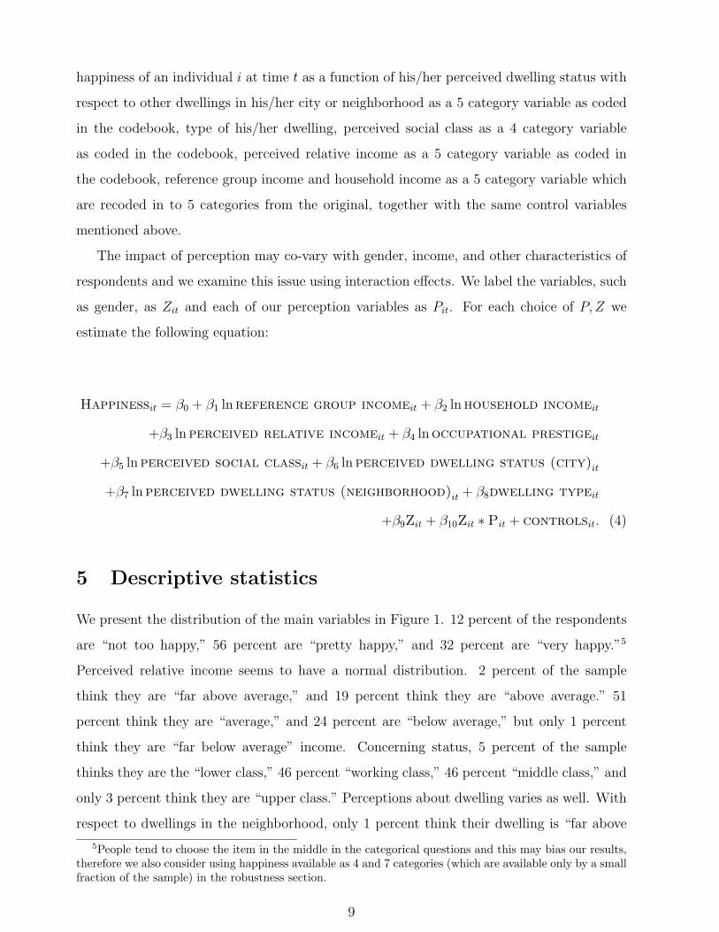
5 Descriptive statistics
We present the distribution of the main variables in Figure 1. 12 percent of the respondents
are “not too happy,” 56 percent are “pretty happy,” and 32 percent are “very happy.”5
Perceived relative income seems to have a normal distribution. 2 percent of the sample
think they are “far above average,” and 19 percent think they are “above average.” 51
percent think they are “average,” and 24 percent are “below average,” but only 1 percent
think they are “far below average” income. Concerning status, 5 percent of the sample
thinks they are the “lower class,” 46 percent “working class,” 46 percent “middle class,” and
only 3 percent think they are “upper class.” Perceptions about dwelling varies as well. With
respect to dwellings in the neighborhood, only 1 percent think their dwelling is “far above
5People tend to choose the item in the middle in the categorical questions and this may bias our results,therefore we also consider using happiness available as 4 and 7 categories (which are available only by a smallfraction of the sample) in the robustness section.
9

average,” 15 percent “above average,” 71 percent “average,” 11 percent “below average,”
and 2 percent “far below average.” Perceptions with respect to dwellings in the city appears
to be normally distributed. 3 percent far “above average,” 19 percent “above average,” 56
percent “average,” 19 percent “below average,” and 3 percent “far below average.”
Figure 2 illustrates graphically whether the part of happiness which can not be explained
by the demographic variables is related to perceptions by plotting the residuals from a
regression of happiness on demographic variables against perceptions. Figure 2 shows a
clear pattern of people with higher perceptions reporting higher happiness. We then examine
the evolution of the happiness and perceptions about relative income in the United States
since 1972. We calculate yearly averages of happiness and perceived relative income in the
GSS (25 observations) and plot those against time in Figure 3. There is large variation
both in happiness and perceived relative income which partly lines up with U.S. recessions
although we will not study that issue in detail. There was a sharp increase in happiness
after 1970 for a couple of years and then happiness declined a little bit but increased again
until 1980. Overall, happiness appears to go up from 1970s to 1980s in the GSS. However,
happiness decreased from 1980 until mid 1980s and then went up until 1990s. The evolution
of happiness between 1990 and 2000 is similar to the one between 1980 and 1990. The
lowest levels of happiness were experienced around 1985 and 1995 and the highest was
experienced around 1988. Around 1982, we observe a huge decline in perceptions about
relative income with a sharp increase in the following years. Perceptions about relative
income are highest around 1975 and lowest around 1982. Overall, perceptions about relative
income and happiness appear to move hand to hand most of the time.
Table 1 considers perceived income rankings and happiness and we observe a positive
relationship between perceptions of relative income and happiness. Table 2 reveals a positive
relationship between perceptions about one’s social class and happiness. Perceived relative
income is, not surprisingly, closely related to actual relative income as can be seen from
Table 3. Interestingly, a large number of individuals perceive themselves to have average
income, almost independently of their actual income; for example, 44 percent of individuals
with actual income far below average consider themselves to have “average” income while
49 percent of individuals with actual income far above average consider themselves to have
“average” income.
Table 4 shows that the correlation between actual and perceived relative income is posi-
10

tive at 0.48. The correlation between actual income and reference group income is 0.67 and
the correlation between perceived relative income and reference group income is quite low
at 0.36. The lack of perfect correlation allows us to estimate the impact of perceived and
actual income ranking simultaneously and evaluate if both matter for happiness and which
one is more important. Perceived social status is correlated with perceived relative income
at 0.37 but much less so with reference group income at 0.26. Perceived social status is posi-
tively correlated with actual social status but this correlation is also low at 0.27. Household
income is positively correlated with perceived social status with a correlation of 0.33. Per-
ceptions about relative income during childhood, as expected, have the highest correlation
with current perceptions about relative income but this number is only 0.19.
6 Empirical results
Table 5 presents OLS estimates and t-statistics for our baseline specification. We find that
income positively relates to happiness with a t-statistic of almost 15.6 However, reference
group income has a significant negative influence on happiness. One point increase in ln
reference group income leads to a 0.015 point reduction in happiness. Dwelling ownership
correlates happiness as renters are 0.024 points less happy than house owners. Employment
status also significantly affects happiness (the omitted category is the working category);
however, we do not find any significant impact of working hours on happiness. Unemployed
are 0.139 points “less happy than employed individuals and people out of the labor force are
happier than those who are working.7 Females are 0.045 points happier than males consistent
with most studies around the world.
Happiness is non-linear in age—increasing at early ages and then decreasing but at a
decreasing rate and blacks are very significantly less happy than whites. We see a significant
effect of education on happiness with one more year of education associated with a 0.011
points increase in happiness. Household size is negatively correlated with happiness while
marital status is a very strong predictor of happiness according to Table 5 (the omitted
category is not being married). Married are 0.249 points happier than nonmarried.
6We use real income in all our regressions—Winkelmann et al. (2007b) show that there is no moneyillusion with respect to individual satisfaction.
7Winkelmann et al. (2007a) show that well-being from working in ones chosen job may be higher ratherthan from in any random job.
11

Concerning religious preferences, Protestants, Orthodox-Christians, and Christians are
happier than Catholics (omitted category); however, Jewish, Buddhists, non religious, and
adherents of Native American religions are less happy than Catholics. Living in a big city
is correlated with less happiness and a one point increase in ln local population leads to a
0.008 point decrease in happiness.
We estimate the baseline regression separately for non-married and married. Income
comparisons are more important for married but the positive influence of income on happiness
is larger for nonmarried and dwelling ownership appears to be more important for nonmarried
as well. Being unemployed, or not in the labor force, affects happiness more for married while
it appears that the female-male happiness gap decreases with marriage. Married blacks are
much less happy than single blacks. The influence of education on happiness is two times
higher for nonmarried while the influence of religion on happiness is higher for married. For
instance, among nonmarried, non-religious are 0.049 points less happy than Catholics and
this number increases to 0.088 for married. The negative influence of city size on happiness
for the married sample is similar to the one for the nonmarried sample. Lastly, happiness
responses are explained better by the independent variables for nonmarried as suggested by
a higher adjusted R-squared.
Tables 6 and 7 focus on our main task; namely, estimating the contributions of income,
relative income, and perceptions to happiness. In order to hedge against spurious conclu-
sions due to potentially erroneous assumptions of linearity, we present the results from two
specifications—one where income is measured as a “continuous” variable (in Tables 6 and
7) and one where we use dummy variables for income categories and perceptions (Table 8).
In these tables we, for brevity, only display the main coefficients of interest.
We performed a series of regressions in order to identify the reference group that has
the strongest effect on happiness. We do not report the details but our results indicate
that individuals compare themselves to individuals from their own cohort who work in the
same occupation and live in the same region. By doing a specification search like this we
may overestimate the impact of relative income due to “data mining,” although we may
also underestimate the effect of relative income because we do not really know which groups
individuals compare themselves to. If people, as argued by Gilbert and Trower (1990), choose
whom to compare themselves to, it may be the case that they tend to compare themselves
to individuals that are systematically better or worse off than themselves. If such is the case,
12

then perceived relative income may be a “more correct” measure of relative income than our
measured relative income in a technical sense. However, it is very hard to empirically separate
the case where individuals choose their comparison group from the case where individuals
form imperfect perceptions. We examined if individuals know about other people’s income
with a lag by checking if “reference group income,” defined as the income of the comparison
group one year earlier, is more significant than reference group income calculated from the
current income of the comparison group. We found no evidence of such an information lag
and do not tabulate the results.
We display the coefficients to actual income, reference group income, perceived relative
income, and social status while suppressing those of demographic variables. In Table 6, we
use ln values of our main variables and both actual income and reference group income are
significant. However, the coefficient to perceived relative income is four times that of the
coefficient to actual income and 12 times that of reference group income. This coefficient is
estimated with an extremely high level of significance with a t-statistic of 27. In the second
column, we include occupational prestige but it is not significant. In the third column, we
include perceived social class which is a strongly significant predictor of happiness with a
t-statistic of 11.4.8 The inclusion of this variable lowers the significance of perceived relative
income, as one might expect, but this reduction is quite small. It appears that perceived
relative income and perceived social class have separate strong impacts on happiness.
In Table 7, we investigate the role of perceptions about own dwelling. We use two
variables: perceptions with respect to other dwellings in the city and perception with respect
to other dwellings in the neighborhood. The reference group is much more clearly stated for
these variables. Perceived dwelling status relative to other dwellings in the city is significantly
and positively correlated with happiness after controlling for dwelling ownership and dwelling
type. In the second column, we include perceived dwelling status relative to other dwellings in
the neighborhood and find a larger, more significant, coefficient. This result clearly supports
Luttmer’s (2005) notion of “neighbors as negatives” in the sense that observable well-being
of neighbors can lower happiness.
In Table 8, we enter income, status, and perception variables as dummy variables. Such a
specification does not impose the restriction that the change in happiness when moving from
8We still include occupational prestige in column 3 and in all regressions where perceived social classenters as a correlate of happiness in the rest of the paper. However, we do not report the coefficients sincethey are not significant as one may expect from the results in the second column of Table 6.
13

one level of, say, income to a higher level of ln income is the same for all levels of income as
does the log-linear specification in the previous table. We find that all categories of income
are significant in explaining happiness. Reference group income has a significant and negative
effect only for the “far above average” category while perceived relative income has a positive
effect with extremely high significance for the “average” and “above average” categories (“far
below average” is the omitted category). Perceived social class is significant at high levels of
significance for all categories (compared to the left-out category “far below average”) with
t-values around 13. Overall, these results provide clear evidence that people’s perceptions
of income and status are highly correlated with happiness. Concerning perceptions about
dwelling, perceptions relative to city dwellings is significant for all categories except “below
average.” Perceptions relative to dwellings in the neighborhood is significant for all categories
in explaining happiness and is a stronger predictor than the former as found above.
Next, in Table 9, we investigate the role of selection. We consider three sub-samples:
people living in the same city since childhood, people living in the same state but in a
different city, and people living in a different state. The results show that perceptions matter
for all three categories. Reference group income and perceived social class has a stronger
effect on happiness for those who have moved; however, the income and happiness correlation
is higher for people who never moved to another city or state. Perceived relative income is
highest in significance and in size of the coefficient for those who remain in their childhood
city. Dwelling perceptions clearly matter more for those not moving, while it appears that
dwelling perceptions do not matter for happiness once people move to another city. In the
bottom row, we use nominal values of income and find results very similar to what we found
using real values.
In Table 10, we add interaction terms with our perceived relative measures (income,
status, dwelling) and find that perceptions about relative income are more important for
low income individuals, females, and conservatives. Perceived social class matters more for
conservatives. Perceptions about own dwelling are more important for happiness of married,
middle income individuals, males, and conservatives while perceptions matter less for people
with higher intelligence as measured by the ability to guess words. Inequality aversion lessens
the influence of perceived income and social class but strengthens the impact of dwelling
perceptions. Hours of TV watched interact positively with dwelling perceptions.9 When we
9We also tried interactions with being self-employed (versus being an employee). We did not find any
14

interact our relative perception measures (income, status, dwelling) with interpersonal trust,
we observe that perceptions matter more for less trusting people. Interestingly, trust matters
most for perceived relative income according to both size and significance of the interaction.
Indeed, the coefficient on the interaction terms between trust and perceived relative income is
three times higher compared with the interaction between trust and perceived dwelling status
(neighborhood and city). Trust matters more for perceived social class than for perceived
dwelling status.
7 Conclusion
High income is correlated with higher levels of happiness but high reference group income is
negatively related to happiness. However, even if income is low in both absolute and relative
terms, happiness is within reach as long a perceived social status or perceived relative income
is high. Perceptions about own dwelling relative to other dwellings are also important for
the well-being reinforcing the conclusion that happiness strongly correlates with perceptions.
significant results when we used our perception variables as continuous variables. However, when we usedperceptions as categorical variables, we found significant interaction effects only for perceived relative income.
15

References
[1] Blanchflower, D.G.,& Oswald, A.J. (2000a). The Rising Well-Being Of the Young.
NBER Working Paper No. 6102.
[2] Blanchflower, D.G.,& Oswald, A.J. (2000b). Well-Being Over Time In Britain and the
U.S.A. NBER Working Paper No. 7787.
[3] Clark, A.E.,& Oswald, A.J. (1994). Unhappiness and Unemployment. Economic Journal
104, 648-659.
[4] Clark, A.E., Frijters, P.,& Shields, M.A. (2008). Relative Income, Happiness and Utility:
An Explanation For the Easterlin Paradox and Other Puzzles. Journal of Economic
Literature 46, 95-144.
[5] Clark, A.E., Kristensen, N., & Westerg̊ard-Nielsen, N. (2009). Economic Satisfaction
and Income Rank In Small Neighbourhoods. Journal of the European Economic Asso-
ciation 7, 519-527.
[6] Clark, A.E., Oswald, A.J. (1996). Satisfaction and Comparison Income. Journal of
Public Economics 61, 359-381.
[7] Clark, Andrew E.,& Senik, C. (2010). Who Compares To Whom? The Anatomy Of
Income Comparisons In Europe. The Economic Journal 120, 573-594.
[8] DiTella, R., Haisken-De-New, J., & MacCulloch, R. (2010). Happiness Adaptation To
Income and To Status In An Individual Panel. Journal of Economic Behavior and
Organization forthcoming.
[9] Duesenberry, J. (1949). Income, Savings and the Theory Of Consumer Behaviour. Cam-
bridge, Mass: Harvard University Press.
[10] Easterlin, R.A. (1963). Towards A Socio-economic Theory Of Fertility: A Survey Of
Recent Research On Economic Factors In American Fertility. In S.J. Behrman, L. Corsa
Jr., R.Freedman (Eds.) Fertility and Family Planning: A World View 127-156. Ann
Arbor: University of Michigan Press.
16

[11] Easterlin, R.A. (1973). Relative Economic Status and the American Fertility Swing. In
E.B. Sheldon (Ed.). Family Economic Behavior: Problems and Prospects, Philadelphia:
J.B. Lippincott for Institute of Life Insurance.
[12] Freedman, D.S. (1963). The Relation Of Economic Status On Fertility. American Eco-
nomic Review 53, 414-426.
[13] Frey, S.B., & Stutzer, A. (2002). What Can Economists Learn From Happiness Research.
Journal of Economic Literature 40, 402-435.
[14] Frijters, P., & Ferrer-i-Carbonell, A. (2003). How Important Is Methodology For the
Estimates Of the Determinants Of Happiness? The Economic Journal 114, 641-659.
[15] Gilbert, P., & Trower, P. (1990). The Evolution and Manifestation Of Social Anxiety. In
R.W. Crozier (Ed.). Shyness and Embarrassment: Perspectives from Social Psychology,
144-177. New York: Cambridge University Press.
[16] Graham, C. (2004). Can Happiness Research Contribute to Development Economics?
Washington DC: The Brookings Institution.
[17] Luttmer, E. (2005). Neighbors As Negatives: Relative Earnings and Well-Being. Quar-
terly Journal of Economics 120, 963-1002.
[18] Moller, V. (1989). Can’t Get No Satisfaction. Indicator South Africa 7, 43-46.
[19] Oswald, J.A. (1997). Happiness and Economic Performance. Economic Journal 107,
1815-1831.
[20] Rablen, M.D. (2008). Relativity, Rank and the Utility Of Income. The Economic Jour-
nal 118, 801-821.
[21] Senik, C. (2009). Direct Evidence On Income Comparison and Their Welfare Effects.
Journal of Economic Behavior and Organization forthcoming.
[22] Van Praag, B.M.S., & Kapteyn, A. (1973). Wat Is Ons Inkomen Ons Waard? (How Do
We Value Our Income?) Economisch Statistische Berichten 58, 360-382.
[23] Wachter, M.L. (1972). A Labor Supply Model For Secondary Workers. The Review of
Economics and Statistics 54, 141-151.
17

[24] Wachter, M.L. (1974). A New Approach To the Equilibrium Labor Force. Economica
41, 35-51.
[25] Winkelmann, R., Luechinger, S., Stutzer, A. (2007a). The Happiness Gains From Sort-
ing and Matching In the Labor Market. University of Zurich Working Paper.
[26] Winkelmann, R., Boes, S. & Lipp, M. (2007b). Money Illusion Under Test. Economics
Letters 94, 332-337.
[27] Winkelmann, R., Boes, S. & Staub, K. (2007c). The Hidden Cost Of Parental Income:
Why Less May Be More. University of Zurich Working Paper.
[28] Wright, S.C. (1985). Health Satisfaction: A Detailed Test Of the Multiple Discrepancies
Theory Model. Social Indicators Research 17, 299-313.
18

(a)
(b) (c)
(d) (e)
Figure 1: Distribution of the main variables (whole sample)
19

(a) perceived relative income (b) perceived social class
(c) perceived dwelling status/neighborhood (d) perceived dwelling status/city
Figure 2: Residual happiness by main variables (whole sample)
20

(a) time series of perceived relative income (b) time series of happiness
Figure 3: Yearly averages
21

Table 1: Descriptive statistics: Perceptions about relative income and happiness
happiness: low middle high total
perceived relative income:far below average 32 49 19 2222below average 19 58 23 10090average 10 57 33 21821above average 6 52 42 7920far above average 11 46 43 834
Notes: This table shows happiness of individuals by perceptions about relative income. Perceived relativeincome is a categorical variable taking values 1-5.
Table 2: Descriptive statistics: Perceptions about social class and happiness
happiness: low middle high total
perceived social class:lower class 33 51 16 2205working class 13 60 27 19067middle class 9 54 37 18923upper class 10 43 47 1344
Notes: This table shows happiness of individuals by perceptions about social class. Perceived social class isa categorical variable taking values 1-4.
22

Table 3: Descriptive statistics: Relation between income and perceptions aboutrelative income
perceived relative income: far below below average above far aboveaverage average average average
income:far below average 9 41 44 4 2below average 4 27 59 10 0average 3 5 52 38 2above average 1 4 40 48 7far above average 2 19 49 28 2
Notes: Numbers are row percentages. Income is recoded into five categories from the original data containing13 categories. Perceived relative income is 5 categories: “far below average,” “below average,” “average,”“above average,” and “far above average.”
Table 4: Correlation matrix: Main variables
household reference perceived occupational perceived perceivedincome group relative prestige social relative
income income class incomewhen 16years old
household income 1.00reference group income 0.67 1.00perceived relative income 0.48 0.36 1.00occupational prestige 0.34 0.38 0.23 1.00perceived social class 0.33 0.26 0.37 0.27 1.00perceived relative income 0.16 0.14 0.19 0.16 0.18 1.00when 16 years old
Notes: All variables are in ln. Perceived relative income is 5 categories: “far below average,” “below average,”“average,” “above average,” and “far above average.” Perceived social class is 4 categories: “lower class,”“working class,” “middle class,” and “upper class.” Occupational prestige takes values 0-100.
23

Table 5: Baseline regressions
Dependent Variable: Self-reported Happiness
OLS(1) (2) (3)
baseline married nonmarried
ln reference group income -0.015 (2.1) -0.027 (2.5) -0.011 (1.7)ln household income 0.077 (15.1) 0.108 (11.3) 0.060 (12.2)rent dwelling -0.024 (2.4) -0.021 (1.4) -0.032 (2.8)ln weekly working hours -0.009 (0.7) -0.012 (1.0) 0.014 (0.8)unemployed -0.139 (4.7) -0.171 (3.6) -0.108 (4.2)not in the labor force 0.055 (5.1) 0.073 (2.9) 0.032 (1.6)female 0.045 (5.9) 0.023 (2.9) 0.046 (3.9)age -0.011 (6.8) -0.007 (3.9) -0.017 (13.3)age-squared/100 0.012 (7.9) 0.008 (4.4) 0.002 (12.7)black -0.119 (16.4) -0.153 (14.3) -0.087 (10.3)not white or black -0.021 (1.1) -0.009 (0.4) -0.042 (2.9)years of education 0.011 (10.6) 0.008 (4.1) 0.016 (16.1)ln household size -0.014 (2.4) -0.048 (2.4) -0.002 (0.2)not married (omitted)married 0.249 (31.5)Catholic (omitted)Protestant 0.025 (2.6) 0.028 (2.5) 0.016 (1.5)Jewish -0.083 (3.2) -0.052 (1.6) -0.129 (4.0)No religion -0.064 (7.9) -0.088 (4.2) -0.049 (4.4)Other religions -0.026 (1.2) -0.021 (1.0) -0.037 (1.1)Buddhist -0.121 (2.6) -0.054 (0.4) -0.149 (1.8)Hindu -0.049 (0.7) 0.002 (0.1) -0.153 (1.9)Other eastern religions -0.061 (0.2) -0.069 (0.2) -0.087 (0.3)Muslim 0.157 (1.3) 0.188 (1.2) 0.082 (0.6)Orthodox-Christian 0.182 (2.5) 0.227 (2.7) 0.089 (1.1)Christian 0.075 (1.5) 0.133 (2.7) 0.015 (0.3)Native American religions -0.287 (5.8) -0.652 (1.9) -0.171 (1.1)Inter-nondenominational 0.043 (0.9) 0.060 (0.6) 0.017 (0.2)ln place population -0.008 (7.7) -0.007 (4.5) -0.009 (5.3)region fixed effects Yes Yes Yesyear fixed effects Yes Yes Yesoccupation fixed effects Yes Yes Yesindustry fixed effects Yes Yes Yes
Adjusted R-squared 0.0917 0.0428 0.0516Number of observations 43317 24249 19062
Notes: We estimate Equation 1 using OLS for the whole sample in column (1). We estimate self-reportedhappiness of an individual i at time t as a function of his/her ln reference group income and ln householdincome together with the following controls variables: dwelling ownership, ln weekly working hours, laborforce status, sex, age, age square, race, years of education, ln household size, marital status, religion, lnpopulation of the place of residence, region fixed effects, year fixed effects, occupation fixed effects, andindustry fixed effects. ln reference group income is the ln average income of people who live in the sameregion, work in the same occupation category (1-digit) and are at the same age with the respondent. Incolumn (2), we estimate the same equation only for the married sample, and in column (3), the estimation isdone only for the nonmarried sample. Self-reported happiness is measured on a scale 1-3 which correspondsto: “very happy,” “pretty happy,” and “not too happy.” t-statistics in absolute values are reported inparentheses. Robust standard errors are used.
24

Table 6: The role of perceptions about relative income and status
Dependent Variable: Self-reported Happiness
OLS(1) (2) (3)
main variables� coeff. t-stat. coeff. t-stat. coeff. t-stat.ln reference group income -0.021 2.7 -0.023 2.9 -0.023 3.0ln household income 0.070 11.9 0.070 11.7 0.063 11.3ln perceived relative income 0.258 27.2 0.256 28.6 0.217 21.4ln occupational prestige 0.012 0.7 0.010 0.6ln perceived social class 0.189 11.4
Adjusted R-squared 0.0802 0.0825 0.0882Number of observations 43317 43317 43317
Notes: OLS regressions. In column (1), we estimate Equation 2 and present the coefficients for the mainvariables of interest. We estimate self-reported happiness of an individual i at time t as a function of his/her lnperceived relative income, ln reference group income and ln household income together with the same controlvariables used in Table 5, column 1. Perceived relative income is the answer to the question, “Comparedwith American families in general, would you say your family income is far below average, below average,average, below average, or far above average?” Perceived relative income takes the values 1-5 and treated asa continuous variable in this estimation. In column (2), we estimate self-reported happiness of an individuali at time t as a function of his/her ln occupational prestige, ln perceived relative income, ln referencegroup income and ln household income together with the same control variables used in Table 5, column1. Occupational prestige takes values 0-100 where higher values correspond to higher occupational prestige.In column (3), we estimate self-reported happiness of an individual i at time t as a function of his/her lnperceived social class, ln occupational prestige, ln perceived relative income, ln reference group income and lnhousehold income together with the same control variables used in Table 5, column 1. Perceived social statusis the answer to the question, “If you were asked to one of four names for your social class, which would yousay you belong in? The lower class, the working class, the middle class, or the upper class?” It takes values1-4 and is treated as a continuous variable in the estimation. Self-reported happiness is measured on a scale1-3 which corresponds to: “very happy,” “pretty happy,” and “not too happy.” t-statistics are reported inabsolute values. Robust standard errors are used.
25

Table 7: Comparing dwelling to others in the neighborhood and the city
Dependent Variable: Self-reported Happiness
OLS(1) (2)
main variables� coeff. t-stat. coeff. t-stat.ln reference group income -0.024 2.9 -0.022 2.8ln household income 0.062 11.6 0.064 12.6ln perceived relative income 0.216 20.9 0.217 20.1ln perceived social class 0.189 11.1 0.193 11.5ln perceived dwelling status (city) 0.082 2.1ln perceived dwelling status (neighborhood) 0.118 4.2dwelling type dummies Yes Yes
Adjusted R-squared 0.0851 0.0852Number of observations 43317 43317
Notes: OLS regressions. In column (1), we estimate Equation 5 and present the coefficients only for themain variables. We estimate self-reported happiness of an individual i at time t as a function of his/herln perceived dwelling status with respect to other dwellings in his/her city, type of his/her dwelling, lnperceived social class, ln occupational prestige, ln perceived relative income, ln reference group income andln household income together with the same control variables used in Table 5, column 1. Perceived dwellingstatus (city) is the answer to the question, “Compared to apartments/houses in the city, would you say thehouse/apartment was...” and the answer is a categorical variable which is “far below average” (1), “belowaverage” (2), “average” (3), “above average” (4), “far above average” (5), and no answer (missing), notapplicable (missing). It takes values 1-5 and is treated as a continuous variable in the estimation. In column(2), we estimate Equation 6 using and present the coefficients only for the main variables of interest. Weestimate self-reported happiness of an individual i at time t as a function of his/her ln perceived dwellingstatus with respect to other dwellings in his/her neighborhood, type of his/her dwelling, ln perceived socialclass, ln occupational prestige, ln perceived relative income, ln reference group income and ln householdincome together with the same control variables used in Table 5, column 1. Dwelling type is the same asexplained above. Perceived dwelling status (neighborhood) is the answer to the question, “Compared toapartments/houses in the neighborhood, would you say the house/apartment was...” and the answer is acategorical variable which is; “far below average” (1), “below average” (2), “average” (3), “above average”(4), “far above average” (5), and no answer (missing), not applicable (missing). It takes values 1-5 and istreated as a continuous variable in the estimation. Self-reported happiness is measured on a scale 1-3 whichcorresponds to: “very happy,” “pretty happy,” and “not too happy.” t-statistics are reported in absolutevalues. Robust standard errors are used.
26

Table 8: Nonlinearities in perceptions
Dependent Variable: Self-reported Happiness
OLS(1) (2)
main variables� coeff. t-stat. coeff. t-stat.reference group income: (omitted) far below average
below average -0.002 0.3 -0.002 0.4average -0.009 0.8 -0.009 0.7
above average -0.004 0.4 -0.004 0.5far above average -0.014 2.1 -0.014 2.2
household income: (omitted) far below averagebelow average 0.017 1.8 0.018 1.8
average 0.045 3.6 0.045 3.7above average 0.045 3.3 0.045 3.3
far above average 0.085 6.7 0.085 6.9perceived relative income: (omitted) far below average
below average 0.090 4.1 0.090 4.0average 0.212 13.5 0.212 13.8
above average 0.249 13.7 0.249 13.8far above average 0.227 4.9 0.227 4.9
perceived social class: (omitted) below averageaverage 0.143 12.9 0.144 13.4
above average 0.210 13.7 0.210 14.0far above average 0.306 11.6 0.306 11.8
perceived dwelling status (city): (omitted) far below averagebelow average 0.040 0.8
average 0.063 2.0above average 0.071 1.5
far above average 0.091 1.9perceived dwelling status (neighborhood): (omitted) far below average
below average 0.112 1.4average 0.087 2.7
above average 0.087 2.1far above average 0.212 6.1
R-squared 0.1082 0.1084No. of obs. 43317 43317
Notes: OLS regressions. In column (1), we estimate Equation 3 and present the coefficients for the mainvariables. We estimate self-reported happiness of an individual i at time t as a function of his/her perceiveddwelling status with respect to othe dwellings in his/her city as a 5 category variable as coded in thecodebook, type of his/her dwelling, perceived social class as a 4 category variable as coded in the codebook,perceived relative income as a 5 category variable as coded in the codebook, reference group income andhousehold income as a 5 category variable and are recoded in to 5 categories from the original, together withthe same control variables used in Table 5 column 1. In column (2), we estimate self-reported happiness ofan individual i at time t as a function of his/her perceived dwelling status with respect to other dwellings inhis/her neighborhood as a 5 category variable as coded in the codebook, type of his/her dwelling, perceivedsocial class as a 4 category variable as coded in the codebook, perceived relative income as a 5 categoryvariable as coded in the codebook, reference group income and household income as a 5 category variableand are recoded in to 5 categories from the original, together with the same control variables used in Table 5,column 1. Self-reported happiness is measured on a scale 1-3 which corresponds to: “very happy,” “prettyhappy,” and “not too happy.” t-statistics are reported in absolute values. Robust standard errors are used.
27

Tab
le9:
Test
ing
for
sele
ctio
n
Dep
end
ent
Vari
ab
le:
Sel
f-re
port
edH
ap
pin
ess
main
vari
ab
les⇒
refe
ren
ceh
ou
seh
old
per
ceiv
edp
erce
ived
per
ceiv
edp
erce
ived
Nin
com
ein
com
ere
lati
ve
soci
al
dw
ellin
gd
wel
lin
gver
sus
inco
me
class
statu
sst
atu
sA
dj.R
2
city
nei
ghb
orh
ood
Sp
ecifi
cati
on�
1)
base
lin
e-0
.017
(2.2
)0.0
36
(6.9
)0.2
02
(18.5
)0.1
93
(11.7
)0.0
74
(2.0
)0.0
97
(3.3
)43317/0.1
067
2)
sam
eci
ty-0
.015
(1.6
)0.0
37
(4.0
)0.2
26
(24.5
)0.1
82
(10.5
)0.1
23
(2.8
)0.1
70
(3.8
)17778/0.1
193
3)
sam
est
ate
-0.0
18
(1.8
)0.0
40
(3.4
)0.2
04
(10.4
)0.1
89
(14.5
)0.0
37
(0.8
)0.0
17
(0.5
)10900/0.1
012
diff
eren
tci
ty4)
diff
eren
tst
ate
-0.0
20
(1.9
)0.0
27
(3.1
)0.1
77
(6.6
)0.2
06
(6.2
)0.0
10
(0.2
)0.0
59
(1.5
)14137/0.1
035
5)
nom
inal
vari
ab
les
-0.0
20
(2.6
)0.0
36
(7.5
)0.2
03
(17.8
)0.1
94
(11.9
)0.0
74
(1.9
)0.0
98
(3.3
)43317/0.1
068
Not
es:
OL
Sre
gres
sion
s.E
very
row
wit
ha
num
ber
corr
espo
nds
toa
diffe
rent
regr
essi
on.
Inro
w(1
),w
ees
tim
ate
Equ
atio
n3
and
pres
ent
the
coeffi
cien
ts.
Inro
w(2
),w
eus
eth
esa
mpl
eof
peop
lew
hoha
vebe
enliv
ing
inth
esa
me
city
sinc
ech
ildho
od.
Inro
w(3
),w
eus
eth
esa
mpl
eof
peop
lew
hoha
vebe
enliv
ing
inth
esa
me
stat
ebu
tin
adi
ffere
ntci
tysi
nce
child
hood
.In
row
(4),
we
use
the
sam
ple
ofpe
ople
who
have
been
livin
gin
adi
ffere
ntst
ate
then
the
one
duri
ngch
ildho
od.
Inro
w(5
),w
eus
eno
min
alva
lues
ofho
useh
old
inco
me
and
refe
renc
egr
oup
inco
me.
Inal
lsp
ecifi
cati
ons,
we
disp
lay
the
coeffi
cien
tson
the
mai
nva
riab
les
ofin
tere
st.
The
depe
nden
tva
riab
leis
self-
repo
rted
happ
ines
san
dis
mea
sure
don
asc
ale
1-3
whi
chco
rres
pond
sto
:“v
ery
happ
y,”
“pre
tty
happ
y,”
and
“not
too
happ
y.”
t-st
atis
tics
are
repo
rted
inpa
rent
hese
san
din
abso
lute
valu
es.
Rob
ust
stan
dard
erro
rsar
eus
ed.
Mob
ility
isth
ean
swer
toth
equ
esti
on“W
hen
you
wer
e16
year
sol
d,w
ere
you
livin
gin
this
sam
e(c
ity/
tow
n/co
unty
)?”
Ans
wer
s:“s
ame
stat
e,sa
me
city
”(1
),“s
ame
stat
e,di
ffere
ntci
ty”
(2),
and
“diff
eren
tst
ate”
(3).
28

Tab
le10
:In
tera
ctio
neff
ect
s
Dep
end
ent
Vari
ab
le:
Sel
f-re
port
edH
ap
pin
ess
Pit⇒
per
ceiv
edp
erce
ived
per
ceiv
edp
erce
ived
rela
tive
soci
al
dw
ellin
gd
wel
lin
gin
com
ecl
ass
statu
sst
atu
sci
tyn
eighb
orh
ood
Zit
�1)
marr
ied
0.0
23
(0.9
)0.0
12
(1.1
)0.0
15
(1.9
)0.0
13
(1.6
)2)
low
hou
seh
old
inco
me
(om
itte
d)
mid
dle
hou
seh
old
inco
me
0.0
18
(0.6
)0.0
25
(1.2
)0.0
14
(1.7
)0.0
12
(1.5
)h
igh
hou
seh
old
inco
me
-0.0
87
(6.6
)-0
.019
(1.3
)0.0
03
(0.3
)0.0
08
(0.8
)3)
fem
ale
0.0
29
(2.1
)0.0
02
(0.1
)-0
.015
(2.2
)-0
.017
(2.4
)4)
nu
mb
erof
word
sgu
esse
d-0
.001
(1.9
)-0
.002
(1.8
)-0
.005
(4.3
)-0
.005
(3.7
)5)
red
uce
inco
me
diff
eren
ces
-0.0
04
(3.6
)-0
.013
(3.2
)0.0
09
(3.4
)0.0
08
(3.2
)6)
politi
cal
vie
w0.0
2(3
.5)
0.0
06
(4.1
)0.0
05
(3.1
)0.0
05
(2.8
)7)
soci
alize
wit
hn
eighb
ors
0.0
17
(2.8
)0.0
13
(2.9
)0.0
13
(2.1
)0.0
09
(2.3
)8)
soci
alize
wit
hfr
ien
ds
0.0
24
(3.4
)0.0
14
(3.4
)0.0
01
(0.1
)0.0
08
(0.6
)w
ho
are
not
nei
ghb
ors
9)
soci
alize
wit
hre
lati
ves
0.0
24
(3.0
)0.0
11
(2.2
)0.0
17
(1.5
)0.0
12
(1.6
)10)
hou
rsof
TV
watc
hin
g-0
.009
(0.7
)-0
.011
(1.9
)0.0
09
(1.8
)0.0
13
(3.2
)11)
tru
stp
eop
le(o
mit
ted
)ca
nn
ot
tru
stp
eop
le0.1
05
(6.6
)0.0
47
(2.8
)0.0
29
(4.6
)0.0
21
(2.9
)d
epen
ds
0.0
89
(2.6
)0.0
72
(2.1
)0.0
67
(2.2
)0.0
69
(2.3
)
Not
es:
OL
Sre
gres
sion
s.W
ees
tim
ate
Equ
atio
n4
and
pres
ent
the
coeffi
cien
tson
the
inte
ract
ion
term
sbe
twee
ndi
ffere
ntva
riab
les
(Zit
:va
riab
les
inth
efir
stco
lum
nin
the
tabl
ew
hich
are
num
bere
d1-
12)
and
one
ofou
rpe
rcep
tion
vari
able
s(P
it:
lnpe
rcei
ved
rela
tive
inco
me,
lnpe
rcei
ved
soci
alcl
ass,
lnpe
rcei
ved
dwel
ling
stat
us(c
ity)
and
lnpe
rcei
ved
dwel
ling
stat
us(n
eigh
borh
ood)
).T
hede
pend
ent
vari
able
isse
lf-re
port
edha
ppin
ess
and
ism
easu
red
ona
scal
e1-
3w
hich
corr
espo
nds
to:
“ver
yha
ppy,
”“p
rett
yha
ppy,
”an
d“n
otto
oha
ppy.
”R
obus
tst
anda
rder
rors
are
used
and
t-st
atis
tics
are
repo
rted
inpa
rent
hese
s.In
row
(1),
mar
ried
isa
dum
my
vari
able
taki
ngth
eva
lue
1if
ape
rson
ism
arri
ed,
0ot
herw
ise
(sin
gle,
wid
ow(e
r),
ordi
vorc
ee).
Inro
w(2
),ho
useh
old
inco
me
isco
ded
inth
ree
grou
psan
dis
used
asa
cate
gori
calv
aria
ble.
Inro
w(3
),ge
nder
dum
mie
sar
eus
edan
dm
ale
isth
eom
itte
dca
tego
ry.
Inro
w(4
),nu
mbe
rof
wor
dsgu
esse
dis
the
scor
efr
oma
test
inG
SSth
ata
pers
onge
tsfo
rco
rrec
tly
gues
sing
som
eun
know
nw
ords
.In
row
(5),
“red
uce
inco
me
diffe
renc
es”
isth
ean
swer
toth
equ
esti
on“H
owm
uch
gove
rnm
ent
shou
ldre
duce
inco
me
diffe
renc
es?”
and
ism
easu
red
ona
scal
e1-
7(1
=“n
ogo
vern
men
tac
tion
,”7=
“gov
ernm
ent
shou
ld.”
).In
row
(6),
polit
ical
view
ism
easu
red
ona
scal
e1-
7w
here
1is
“ext
rem
ely
liber
al,”
and
7is
“ext
rem
ely
cons
erva
tive
.”In
row
(11)
,tr
ust
take
s3
valu
esan
dis
used
asa
cate
gori
cal
vari
able
;“t
rust
peop
le,”
“can
not
trus
tpe
ople
,”an
d“d
epen
ds.”
29

8 APPENDIX
ROBUSTNESS TABLES.
We present the summary statistics for the variables used in the paper in Tables A.1 and
A.2. We report the means for the continuous variables (for instance, weekly working hours)
and proportions (for instance, labor force status) for the categorical variables.
We estimate self-reported happiness of an individual i at time t as a function of his/her
ln perceived dwelling status with respect to other dwellings in his/her neighborhood and
city, type of his/her dwelling, ln perceived social class, ln occupational prestige, ln perceived
relative income, ln reference group income and ln household income together with the fol-
lowing controls variables: dwelling ownership, ln weekly working hours, labor force status,
sex, age, age square, race, years of education, ln household size, marital status, religion, ln
population of the place of residence, region fixed effects, year fixed effects, occupation fixed
effects, and industry fixed effects.
Since the question on perceptions about relative income is asked with respect to “Ameri-
can families in general” in the GSS, we use ln GDP per capita as the reference group income
in specification two. ln GDP per capita is negatively and significantly correlated with hap-
piness, as expected, and it does not change any of our results. Then, in column 2, we use ln
sector level (1-digit) wages and ln sectoral level GDP as reference group income. Perception
variables do not change but total sector GDP does not predict happiness. In the fourth
specification, we run an OLS regression of household income on parent’s education, spouse
working hours, spouse labor force status and spouse occupational prestige. Then, we calcu-
late the predicted income for everyone. We do the same in the fifth specification but now we
use interval regression to calculate predicted income (original household income in the GSS is
in intervals). Our results are robust to these cases but now reference group income positively
correlates with happiness. Lastly, we use ln sectoral wage and predicted income together and
again the results do not change. One concern in these regressions can be multi-collinearity.
However, Table A.4 shows that this is not the case and a perfect correlation does not exist
among the independent variables used in the regression in Table A.3.
We conduct robustness checks in several ways in Table A.5. We control for ln personal
income since perceptions might be correlated with personal income instead of household
income. Our results again do not change. In the fourth specification, we estimate our model
30

with ordered probit and find that the coefficients and the t-statistics are quite similar to the
ones with OLS. We estimate our model for married and nonmarried samples and find that
our results are again robust to different sub-samples. Next, we use levels of the income and
status variables instead of logarithms in specification seven. In specifications eight and nine,
we control for own and spouse’s socio-economic status which might affect our main variables
of interest and happiness at the same time. The results again are robust.
We conduct more robustness checks in Table A.6. We use perceived social class as a
10 category variable and then use happiness as a 7 category variable but our results do
not change (these variables are often missing). In the third specification, we consider using
“daily happiness” instead of general happiness. We find that daily happiness is not correlated
with household income nor with actual relative income. However, perceptions about relative
income and social class can predict daily happiness. Moreover, daily happiness is a 4 category
variable which provides an opportunity to control for personal bias in choosing the middle
category in odd numbered questions. In the fourth specification, we use residual happiness
instead of actual happiness as the dependent variable. By doing so, we try to control for
any collinearity problem between income and other variables since residual happiness is
calculated after the regression of happiness on household income and other variables in the
baseline regression. For example, if income aspirations are correlated with perceptions as
well as happiness, this might bias our results. Therefore, we control for income aspirations.
We also use the distance from poverty line as a measure of actual relative income and the
results are robust to this (this variable is generated by the GSS). In addition, we control
for spouse’s work status and use interval regressions to assign income levels from income
intervals, assuming that income is log-normally distributed, rather than taking the midpoint
in their conversion of categorical income categories to point estimates. The results are robust
to these permutations.
It is believed that childhood and past life events have effects on the current well-being
of an individual. These events might also be correlated with perceptions which can bias
our estimates. Therefore, we control for these variables in the regressions in Table A.7. We
find that individuals perceptions about their family income during childhood matters. It
appears that the size of the coefficient on current perceived relative income declines with
the inclusion of perceptions during childhood which suggests that there might be some
persistence in perceptions during the life cycle (One might think of using perceptions during
31

Table A.1: Other independent variables’ means, proportions, and standard deviations
Variable mean stdev
happiness 2.2 0.63ln reference group income 10.6 0.99ln household income 9.9 0.98ln personal income 9.5 1.08perceived relative income 2.9 0.83perceived social class 2.5 0.65perceived relative income 2.8 0.86when 16 years oldage 45.2 17.52own dwelling 62.8 0.04rent dwelling 35.0 0.03other dwelling 2.2 0.01employed 61.9 0.02unemployed 3.0 0.01not in the labor force 35.1 0.02male 43.9 0.02female 56.1 0.02white 82.7 0.02black 13.8 0.02other 3.5 0.01years of education 12.6 3.2children 1.9 1.81household size 2.7 1.54married 55.5 0.02not married 45.5 0.02dwelling relative to neighborhood 3.1 0.62dwelling relative to city 3.0 0.78
Notes: This table shows the summary statistics of the variables used in the paper. Means are reported forthe continuous variables and proportions (for instance, 61.9 equals to the number of people who are employeddivided by the sum of people who are employed, unemployed, and not in the labor force.) are reported forcategorical variables.
childhood as an instrument for current perceptions however the childhood perceptions are
asked currently. Hence, current personal characteristics might influence the answer to this
question. Therefore, we only consider using it as another explanatory variable for the current
well-being.) Considering deaths, hospitalizations and divorces, we find that past events have
strong influence on current happiness however we find evidence for adaptation. For instance,
the influence of death of spouse in the last year is higher than the death fours ago or more
than 6 years ago. Interestingly, people are affected more by the death of the mother than
the father. There seems to be some adaptation to perceptions and also income shocks in the
United States. We only display the coefficients on the extra controls in the table but our
results are robust to the inclusion of past life events.
32

Table A.2: Other independent variables’ means, proportions, and standard deviations
Variable mean stdev
Protestant 60.9 0.02Catholic 24.6 0.02Jewish 21.0 0.01none 9.26 0.01other denominations 1.9 0.01Buddhist 0.1 0.01Muslim 0.1 0.01Orthodox-Christian 0.1 0.01Christian 0.5 0.01Inter-Nondenominational 0.2 0.01mobility:same city 41.4 0.02same state, different city 25.5 0.02different state 33.1 0.02ln occupational prestige 3.7 0.37number of words guessed 6.0 2.16political view 4.1 1.35opinion on income differences 4.3 1.96health 3.0 0.85weekly working hours 41.2 14.07household size 3.5 2.19ln own socio-economic index 3.80 0.40ln spouse socio-economic index 3.84 0.39
Notes: This table shows the summary statistics of the variables used in the paper. Means are reported forthe continuous variables and proportions (for instance, 41.4 equals to the number of people who still livein the same city divided by the sum of people who live in the same city, same state but different city, anddifferent state.) are reported for categorical variables.
33

Tab
leA
.3:
Alt
ern
ati
ve
measu
res
of
house
hold
inco
me
and
refe
rence
gro
up
inco
me
Dep
end
ent
Vari
ab
le:
Sel
f-re
port
edH
ap
pin
ess
main
vari
ab
les⇒
refe
ren
ceh
ou
seh
old
per
ceiv
edp
erce
ived
per
ceiv
edp
erce
ived
inco
me
inco
me
rela
tive
soci
al
dw
ellin
gd
wel
lin
gin
com
ecl
ass
statu
sst
atu
sci
tyn
eighb
orh
ood
Sp
ecifi
cati
on�
1)
lnG
PD
per
cap
ita
as
refe
ren
cegro
up
inco
me
-0.0
40
(2.1
)0.0
48
(12.4
)0.2
16
(20.1
)0.1
92
(12.2
)0.0
81
(2.1
)0.1
18
(4.2
)2)
lnse
ctora
lw
age
as
refe
ren
cegro
up
inco
me
-0.0
04
(1.9
)0.0
24
(5.5
)0.2
02
(18.3
)0.1
93
(11.7
)0.0
71
(2.0
)0.0
95
(3.2
)3)
lnse
ctora
lG
DP
as
refe
ren
cegro
up
inco
me
-0.0
02
(0.9
)0.0
23
(5.1
)0.2
01
(17.3
)0.1
94
(11.8
)0.0
63
(1.9
)0.0
80
(2.7
)4)
pre
dic
ted
hou
seh
old
0.0
09
(1.6
)0.0
57
(4.1
)0.2
09
(18.4
)0.1
92
(11.7
)0.0
74
(2.0
)0.0
99
(3.5
)in
com
eby
OL
Sas
the
hou
seh
old
inco
me
5)
pre
dic
ted
hou
seh
old
inco
me
by
0.0
08
(1.5
)0.0
89
(4.8
)0.2
08
(18.9
)0.1
93
(11.5
)0.0
75
(2.1
)0.1
01
(3.5
)in
terv
al
regre
ssio
nas
the
hou
seh
old
inco
me
6)
2an
d4
-0.0
03
(1.7
)0.0
56
(4.6
)0.2
11
(16.2
)0.1
95
(12.6
)0.0
69
(1.8
)0.0
88
(3.2
)
Not
es:
OL
Sre
gres
sion
s.E
ach
row
wit
ha
num
ber
corr
espo
nds
toa
diffe
rent
regr
essi
on.
Inro
w(1
),w
ees
tim
ate
Equ
atio
nA
.1.
We
use
lnG
DP
per
capi
taas
lnre
fere
nce
grou
pin
com
e.In
row
(2),
we
esti
mat
eE
quat
ion
3us
ing
lnse
ctor
alw
age
asln
refe
renc
egr
oup
inco
me.
Inro
w(3
),w
ew
eus
eln
sect
oral
GD
Pas
refe
renc
egr
oup
inco
me.
Inro
w(4
),w
eus
eln
pred
icte
dho
useh
old
inco
me
asln
hous
ehol
din
com
e.P
redi
cted
hous
ehol
din
com
eis
the
pred
icte
dva
lue
whe
nw
eru
nan
OL
Sre
gres
sion
ofho
useh
old
inco
me
onpa
rent
’sed
ucat
ion,
spou
sew
orki
ngho
urs,
spou
sela
bor
forc
est
atus
and
spou
seoc
cupa
tion
alpr
esti
ge.
Inro
w(5
),w
eus
ean
inte
rval
met
hod
toca
lcul
ate
lnho
useh
old
inco
me
from
the
orig
inal
cate
gori
alin
com
eva
lues
repo
rted
inth
eco
debo
ok.
Inal
lsp
ecifi
cati
ons,
we
disp
lay
the
coeffi
cien
tson
the
mai
nva
riab
les
ofin
tere
st.
The
depe
nden
tva
riab
leis
self-
repo
rted
happ
ines
san
dis
mea
sure
don
asc
ale
1-3
whi
chco
rres
pond
sto
:“v
ery
happ
y,”
“pre
tty
happ
y,”
and
“not
too
happ
y.”
t-st
atis
tics
inab
solu
teva
lues
are
repo
rted
inpa
rent
hese
s.R
obus
tst
anda
rder
rors
are
used
.N
omin
alva
riab
les
are
defla
ted
byC
PI.
34

Table A.4: Correlation of instruments with main variables
ln household ln reference ln perceived ln perceivedincome group relative social
income income class
ln GDP per capita 0.02 0.46 0.02 0.01ln sectoral wage 0.03 0.17 0.01 0.04ln sectoral GDP 0.05 0.19 0.03 0.03
Notes: We show the correlations among the instruments used in Table A.3 and ln household income, lnreference group income, ln perceived relative income, and ln perceived social class. All variables are inlogarithms.
35

Tab
leA
.5:
Robust
ness
check
s:I
Dep
end
ent
Vari
ab
le:
Sel
f-re
port
edH
ap
pin
ess
main
vari
ab
les⇒
refe
ren
ceh
ou
seh
old
per
ceiv
edp
erce
ived
per
ceiv
edp
erce
ived
Nin
com
ein
com
ere
lati
ve
soci
al
dw
ellin
gd
wel
lin
gver
sus
inco
me
class
statu
sst
atu
sA
dj.R
2
city
nei
ghb
orh
ood
Sp
ecifi
cati
on�
1)
base
lin
e-0
.017
(2.2
)0.0
36
(6.9
)0.2
02
(18.5
)0.1
93
(11.7
)0.0
74
(2.0
)0.0
97
(3.3
)43317/0.1
067
2)
contr
ol
ln-0
.022
(2.6
)0.0
67
(10.9
)0.2
17
(20.3
)0.1
92
(11.5
)0.0
84
(2.3
)0.1
20
(4.2
)43317/0.0
850
per
son
al
inco
me
3)
ord
ered
pro
bit
-0.0
40
(2.7
)0.1
18
(11.8
)0.4
04
(19.8
)0.3
61
(12.1
)0.1
59
(2.1
)0.2
29
(4.2
)43317/0.0
465
4)
marr
ied
sam
ple
-0.0
27
(2.0
)0.0
55
(5.2
)0.1
79
(9.3
)0.2
08
(8.4
)0.0
86
(2.4
)0.1
24
(5.1
)24249/
0.0
565
5)
non
marr
ied
sam
ple
-0.0
15
(2.1
)0.0
26
(4.1
)0.2
18
(20.0
)0.1
73
(14.4
)0.0
59
(1.2
)0.0
61
(1.0
)19062/
0.0
737
6)
level
sin
stea
dof
logs
-0.0
17
(5.1
)0.0
71
(6.1
)0.0
83
(18.3
)0.0
85
(11.1
)0.0
33
(2.1
)0.0
41
(3.1
)43317/0.1
049
7)
contr
ol
lnow
n-0
.018
(2.3
)0.0
35
(6.8
)0.2
02
(18.4
)0.1
92
(11.2
)0.0
78
(2.1
)0.1
00
(3.5
)43317/0.1
069
soci
o-e
con
om
icin
dex
8)
contr
ol
lnsp
ou
se-0
.017
(2.1
)0.0
35
(6.5
)0.2
02
(18.4
)0.1
92
(11.6
)0.0
76
(1.9
)0.0
9(3
.2)
43317/0.1
069
soci
o-e
con
om
icin
dex
Not
es:
OL
Sre
gres
sion
sun
less
othe
rwis
eno
ted.
Eac
hro
ww
ith
anu
mbe
rco
rres
pond
sto
adi
ffere
ntre
gres
sion
.In
row
(1),
we
esti
mat
eE
quat
ion
3.In
row
(2),
we
cont
rol
for
lnpe
rson
alin
com
eof
the
resp
onde
nt.
Inro
w(3
),w
eus
eor
dere
dpr
obit
esti
mat
ion
and
pres
ent
mar
gina
leff
ects
.In
row
(4),
we
use
only
for
mar
ried
reps
onde
nts
whi
lero
w(5
)is
esti
mat
edfo
rno
nmar
ried
.In
row
(6),
we
use
the
leve
lof
perc
eive
ddw
ellin
gst
atus
wit
hre
spec
tto
othe
rdw
ellin
gsin
his/
her
city
and
neig
hbor
hood
,pe
rcei
ved
soci
alcl
ass,
perc
eive
dre
lati
vein
com
e,re
fere
nce
grou
pin
com
ean
dho
useh
old
inco
me
inth
ere
gres
sion
(hou
seho
ldin
com
ean
dre
fere
nce
grou
pin
com
ear
edi
vide
dby
100,
000)
.In
row
(7),
we
cont
rol
for
the
lnow
nso
cio-
econ
omic
inde
xw
hich
take
sva
lues
0-10
0an
din
row
(8),
we
also
cont
rol
for
the
lnsp
ouse
’sso
cio-
econ
omic
inde
xw
hich
take
sva
lues
0-10
0.In
all
spec
ifica
tion
s,w
edi
spla
yth
eco
effici
ents
onth
em
ain
vari
able
sof
inte
rest
.T
hede
pend
ent
vari
able
isse
lf-re
port
edha
ppin
ess
and
ism
easu
red
ona
scal
e1-
3w
hich
corr
espo
nds
to:
“ver
yha
ppy,
”“p
rett
yha
ppy,
”an
d“n
otto
oha
ppy.
”
36

Tab
leA
.6:
Robust
ness
check
s:II
Dep
end
ent
Vari
ab
le:
Sel
f-re
port
edH
ap
pin
ess
main
vari
ab
les⇒
refe
ren
ceh
ou
seh
old
per
ceiv
edp
erce
ived
per
ceiv
edp
erce
ived
Nin
com
ein
com
ere
lati
ve
soci
al
dw
ellin
gd
wel
lin
gver
sus
inco
me
class
statu
sst
atu
sA
dj.R
2
city
nei
ghb
orh
ood
Sp
ecifi
cati
on�
1)
lnp
erce
ived
soci
al
-0.0
17
(2.2
)0.0
43
(7.8
)0.2
39
(25.1
)0.1
69
(6.7
)0.0
75
(1.9
)0.0
98
(3.1
)43317/0.1
018
class
(10
cate
gory
)2)
hap
pin
ess
(7ca
tegory
)-0
.025
(0.4
)0.0
86
(1.6
)0.4
31
(3.2
)1160/0.1
194
3)
hap
pin
ess
tod
ay
-0.0
20
(0.6
)0.0
13
(0.5
)0.2
52
(6.3
)0.2
50
(3.3
)3747/0.1
268
(4ca
tegory
)4)
resi
du
al
hap
pin
ess
-0.0
17
(2.3
)0.0
34
(6.6
)0.2
02
(18.5
)0.1
93
(11.7
)0.1
73
(2.1
)0.0
97
(3.3
)43317/0.0
317
5)
contr
ol
for
-0.0
17
(2.2
)0.0
36
(6.9
)0.2
02
(18.9
)0.1
93
(11.7
)0.0
74
(1.9
)0.0
98
(3.2
)24249/
0.1
067
inco
me
asp
irati
on
s6)
pover
tylin
e-0
.011
(1.7
)0.0
02(0
.3)
0.2
13
(18.9
)0.1
97
(11.9
)0.0
77
(2.1
)0.1
01
(3.6
)19062/
0.1
062
inst
ead
of
inco
me
7)
dis
tan
cefr
om
0.2
08
(18.9
)0.1
97
(12.2
)0.0
68
(1.9
)0.0
92
(3.3
)43317/0.1
064
pover
tylin
ein
stea
dof
inco
me
an
dre
fere
nce
inco
me
8)
contr
ol
spou
se-0
.018
(2.4
)0.0
36
(7.5
)0.1
99
(18.2
)0.1
91
(11.8
)0.0
72
(1.9
)0.0
91
(3.2
)43317/
0.1
076
work
statu
s
Not
es:
Eve
ryro
ww
ith
anu
mbe
rco
rres
pond
sto
diffe
rent
OL
Sre
gres
sion
s.In
row
(1),
we
esti
mat
eE
quat
ion
3w
ith
perc
eive
dso
cial
clas
sta
king
10va
lues
inst
ead
of5.
Inro
w(2
),th
ede
pend
ent
vari
able
(hap
pine
ss)
take
s7
valu
esin
stea
dof
3.In
row
(3),
the
depe
nden
tva
riab
le(h
appi
ness
)is
“hap
pine
ssto
day”
inst
ead
of“h
appi
ness
inge
nera
l”an
dta
kes
4va
lues
inst
ead
of3.
Inro
w(4
),th
ede
pend
ent
vari
able
isre
sidu
alha
ppin
ess
calc
ulat
edby
esti
mat
ing
Equ
atio
nA
.1an
dca
lcul
atin
gth
ere
sidu
als.
Inro
w(5
),w
eco
ntro
lfo
rin
com
eas
pira
tion
sof
the
resp
onde
nt.
Inro
w(6
),re
lati
vein
com
eis
calc
ulat
edas
inco
me
rela
tive
toth
epo
vert
ylin
e.In
row
(7),
we
also
cont
rol
for
the
spou
se’s
wor
kst
atus
.In
all
spec
ifica
tion
s,w
edi
spla
yth
eco
effici
ents
ofth
em
ain
vari
able
sof
inte
rest
.
37

Table A.7: Controlling for past life events and adaptation
Dependent Variable: Self-reported Happiness
OLS
control variable � coeff. t-stat.1) ln perceived relative income:current 0.197 18.1when 16 years old 0.057 6.92) ever been divorced or separated:yes (no omitted) -0.024 4.13) hospitalized, disabled last 5 years:prior 4 years (none omitted) -0.025 2.3last year -0.054 2.4both -0.138 6.54) divorced in last 5 years:prior 4 years (none omitted) -0.015 1.1last year -0.074 2.1both -0.080 1.24) relatives died in last 5 years:1 in prior 4 years (none omitted) -0.278 3.32+ in prior 4 years -0.042 3.11 last year -0.079 6.01 last year, 1 in prior 4 years -0.001 0.11 in last year, 2+ prior 4 years -0.122 2.92+ last year -0.079 1.52+ last year, 1 prior 4 years 0.036 0.52+ last year, 2+ prior 4 years -0.272 3.65) relatives died since age 16: 0.006 2.9and prior to last 5 years6) death of father:before respondent 16 (none omitted) -0.001 0.16+ years ago 0.005 0.31-5 years ago -0.003 0.2last year -0.039 1.87) death of mother:before respondent 16 (none omitted) -0.020 1.06+ years ago -0.003 0.31-5 years ago -0.039 2.2last year -0.061 1.88) death of spouse:6+ years ago (none omitted) -0.043 3.21-5 years ago -0.075 2.5last year -0.191 4.79) number of traumatic events in last 5 years:last year -0.088 9.1prior 4 years -0.031 5.1
Notes: Every row with a number corresponds to a different regression. In each row, we estimate Equation 3using OLS adding new control variables. For instance, in row 1, we also control for ln perceived relativeincome when the respondent was 16. In the first specification, we control for father’s and mother’s occupa-tional prestige, region dummies, and type of place lived when respondent was 16 years old. Occupationalprestige scores are variables in logs (original 0-100) and type of place lived is a categorical variable tak-ing 6 values where 1= country nonfarm, 2=farm, 3=town less than 50000 people, 4=50000-250000 people,5=big-city suburb, 6=city more than 250000 people. Traumatic events are defined as unemployment, death,divorce/seperation, or hospitalized/disabled.
38

VARIABLES USED IN THE PAPER:
Self-reported happiness: The answer to question 157 in the 2004 GSS codebook: “Taken all together, how
would you say things are these days—would you say that you are very happy, pretty happy, or not too
happy?” Answer: “not too happy” (1), “pretty happy” (2), “very happy” (3), and “don’t know” (missing),
no answer (missing), not applicable (missing).
Perceived relative income: The answer to question 188 in the 2004 GSS codebook: “Compared with
American families in general, would you say your family income is far below average, below average,
average, above average, or far above average? Probe: Just your best guess.” Answer: “far below average”
(1), “below average” (2), “average” (3), “above average” (4), “far above average” (5), and “don’t know”
(missing), no answer (missing), not applicable (missing).
Perceived relative income when 16 years old: The answer to question 30 in the 2004 GSS codebook:
“Thinking about the time when you were 16 years old, compared with American families in general then,
would you say your family income is far below average, below average, average, above average, or far above
average? Probe: Just your best guess.” Answer: “far below average” (1), “below average” (2), “average”
(3), “above average” (4), “far above average” (5), and “don’t know” (missing), no answer (missing), not
applicable (missing).
Perceived social class: The answer to question 185-A in the 2004 GSS codebook: “If you were asked to use
one of four names for your social class, which would you say you belong in: the lower class, the working
class, the middle class, or the upper class?” Answer: “lower class” (1), “working class,” (2) “middle class,”
(3) “upper class,” (4) and “don’t know” (missing), no answer (missing), not applicable (missing).
Household income: 1) We created a continuous family income variable using the mid-point method to the
the answer to question 37 in the 2004 GSS codebook: “In which of these groups did you total family
income, from all sources, fall last year before taxes, that is? Just tell me the letter.” Answer: Under 1000
(1), 1000-2999 (2), 3000-3999 (3), 4000-4999 (4), 5000-5999 (5), 6000-6999 (6), 7000-7999 (7), 8000-8999
(8), 10000-14999 (9), 15000-19999 (10), 20000-24999 (11), 25000 and over (12), refused (missing), don’t
know (missing), no answer (missing), not applicable (missing). 2) GSS generated, variable number 1437 in
the 2004 GSS codebook, family income on 1972-2004 surveys in constant dollars (base 1986)
Health status: The answer to question 159 in the 2004 GSS codebook: “Would you say your own health,
in general, is excellent, good, fair, or poor?” Answer: “Excellent” (4), “good” (3), “fair” (2), “poor” (1),
and “don’t know” (missing), no answer (missing), not applicable (missing).
Marital status: The answer to question 4 in the 2004 GSS codebook: “Are you currently–married,
widowed, divorced, separated, or have you never been married?” Answer: “married” (1), “widowed” (2),
“divorced” (3), “separated” (4), “never married” (5), and no answer (missing). We recode this variable as
follows: married=1, and not married=2, 3, 4, 5.
39

Labor force status: The answer to question 1 in the 2004 GSS codebook: “Last week were you working
full-time, part-time, going to school, keeping house, or what?” Answer: “working full-time” (1), “working
part-time” (2), “with a job, but not at work because of temporary illness, vacation, strike” (3),
“unemployed, laid off, looking for work” (4), “retired” (5), “in school” (6), “keeping house” (7), “other”
(8), and no answer (missing). We recode this variable as follows: employed=1, 2, 3 unemployed=4, and
not in the labor force=5, 6, 7, 8.
Working hours: The answer to question 1-A in the 2004 GSS codebook: “If working full or part-time: How
many hours did you work last week, at all jobs? ” Answer is the number of hours, no answer (missing), not
applicable (missing).
Sex: The answer to question 23 in the 2004 GSS codebook: Coded by the interviewer. “Male” (1) and
“female” (2).
Race: The answer to question 24 in the 2004 GSS codebook: “What race do you consider yourself?”
Answer: “white” (1), “black” (2), “other” (3), and not applicable (missing).
Education: The answer to question 15 in the 2004 GSS codebook: Coded as the number of years of
schooling (maximum is 20) and don’t know (missing), no answer (missing).
Children: The answer to question 12 in the 2004 GSS codebook: ‘ ‘How many children have you ever had?
Please count all that were born alive at any time (including any had from a previous marriage” Answer: 0,
1, 2, 3, 4, 5, 6, 7, 8 or more, don’t know (missing), no answer (missing).
Age: The answer to question 13 in the 2004 GSS codebook: Coded as the number of years from birth,
don’t know (missing), no answer (missing).
Household size: The answer to question 34 in the 2004 GSS codebook: Coded as the number of household
members (1-16), no answer (missing).
Region: The region of interview, question 51 in the 2004 GSS codebook: New England (1), Middle
Atlantic (2), East North Central (3), West North Central (4), South Atlantic (5), East South Central (6),
West South Central (7), Mountain (8), Pacific (9). (See Question 26 in the 2004 GSS codebook for a listing
of the states within regions.)
Occupational prestige: The prestige scores assigned to occupations were taken from rating systems
developed at (NORC) in a project on occupation prestige directed by Robert W. Hodge, Paul S. Siegel,
and Peter H. Rossi. This concept of prestige is defined as the respondents’ estimation of the social standing
of occupations. The prestige scores in the Hodge-Siegel-Rossi and GSS studies were generated by asking
respondents to estimate the social standing of occupations in a nine-step ladder, printed on cardboard and
presented to the respondent. It is constructed from two variables: 1) Occupational prestige score 1974-1992
on page 54 in the 2004 GSS codebook 2) Occupational prestige score 1992-2004 on page 57 in the 2004
GSS codebook. (See page 2050 for the construction of the prestige scores in the 2004 GSS Appendix.)
40

Occupation: One digit occupation categories for the respondents. It is constructed from two variables: 1)
Occupational classifications 1974-1992 on page 54 in the 2004 GSS codebook 2) Occupational classifications
1992-2004 on page 56 in the 2004 GSS codebook. (See pages 2031 and 2068 for the subcategories of
occupational categories in the 2004 GSS Appendix.)
Industry: One digit industry categories for the respondents. It is constructed from two variables: 1)
Occupational classifications 1974-1992 on page 56 in the 2004 GSS codebook 2) Occupational classifications
1992-2004 on page 57 in the 2004 GSS codebook. (See pages 2055 and 2068 for the subcategories of
occupational categories in the 2004 GSS Appendix.)
TV hours: The answer to question 242 in the 2004 GSS codebook: “On the average day, about how many
hours do you personally watch television?” Answer: number of hours from 0-24, and don’t know (missing),
no answer (missing), not applicable (missing). Reference for the variables and the explanations:
Political view: The answer to question 66-A in the 2004 GSS codebook: “We hear a lot of talk these days
about liberals and conservatives. I am going to show you a seven-point scale on which the views that
people might hold are arranged from extremely liberal–point 1– to extremely conservative–point 7. Where
would you place yourself on this scale?” Answer: “Extremely liberal” (1), “liberal” (2), “slightly liberal”
(3), “moderate, middle of the road” (4), “slightly conservative” (5), “conservative” (6), “extremely
conservative” (7), and “don’t know” (missing), no answer (missing), not applicable (missing).
Socialization variables: The answers to question 173 in the 2004 GSS codebook: “Would you use this card
and tell me which answer comes closest to how often you do the following things?” A)“Spend a social
evening with relatives,” B) “Spend a social evening with someone who lives in your neighborhood,” C)
“Spend a social evening with friends who live outside the neighborhood.” Answer: “Never” (1), “about
once a year” (2), “several times a year” (3), “about once a month” (4), “several months a year” (5), “once
or twice a week” (6), “almost every day” (7), and “don’t know” (missing), no answer (missing), not
applicable (missing).
Dwelling variables: Dwelling type: The variable 1469 (interviewer coded) in the 2004 GSS codebook:
Trailer (1), detached single family house (2), 2-family house, 2 units side by side (3), 2-family house, 2
units one above the other (4), detached 3-4 family house (5), row house (6), apartment house, 3 stories or
less (7), apartment house, 4 stories or more (8), apartment in a partly commercial structure (9), other (10),
don’t know (missing), no answer (missing), not applicable (missing). A): The answers to question 1470-A
in the 2004 GSS codebook: “Compared to apartments/houses in the neighborhood, would you say the
house/apartment was...” B) :The answers to question 1470-B in the 2004 GSS codebook: “Compared to
apartments/houses in the city/town/county, would you say the house was...” Answers: “far below average”
(1), “below average” (2), “average” (3), “above average” (4), “far above average”, and (5), “no answer”
(missing), not applicable (missing). Dwelling own: The answers to question 1471 in the 2004 GSS
codebook: “ (Do you/does your family) own your (home/apartment), pay rent, or what?” Answer: “own or
is buying” (1), “pays rent” (2), “other” (3), and “don’t know” (missing), no answer (missing), not
applicable (missing).
41

Mobility: The answers to question 26-A in the 2004 GSS codebook: “When you were 16 years old, were
you living in this same (city/town/county)?” Answer: “same state, same city” (1), “same state, different
city” (2), “different state” (3), and “don’t know” (missing), no answer (missing).
Religion: The answer to question 104 in the 2004 GSS codebook: “What is your religious preference? Is it
Protestant, Catholic, Jewish, some other religion, or no religion?” Answer: “Protestant” (1), “Catholic”
(2), “Jewish” (3), “none” (4), “other denominations” (5), “Buddhism” (6), “Hinduism” (7), “other
Eastern” (8), “Moslem/Islam” (9), “Orthodox-Christian” (10), “Christian” (11), “Native American” (12),
“Inter-Nondenominational” (13), and “don’t know” (missing), no answer (missing).
Socio-Economic Index scores: Socio-economic indexes of own (variable 1506 in the 2004 GSS codebook)
and the spouse (variable 1510 in the 2004 GSS codebook) taking values 0-100.
Reference for the variables and the explanations:
Webpage: 1972-2004 GSS Codebook http://www.deakin.edu.au/c̃ahit/appendix.pdf
Webpage: 1972-2004 GSS Appendix http://www.deakin.edu.au/c̃ahit/codebook.pdf
42