Subjective Measures of Risk

Eduardo ZambranoDepartment of Economics

Cal PolyMay 20, 2008

Example

• You are offered an investment g where you win $120 with probability ½ and you lose $100 with probability ½.– g is a favorable investment: it’s expected

value is $10.– Should you accept it?

• Better yet, what is the risk in accepting g?

The purpose of this talk

• The problem: How to measure financial risk?– Traditional measures have shortcomings

• Why is the problem important:– Misrepresentation of the risk embedded in an

investment can lead to serious, even catastrophic mistakes in decision making

New solutions

• Aumann and Serrano (AS, 2007)– Measure the risk of g as the number R that

solves E e-g/R =1.

• Foster and Hart (FH, 2007)– Measure the risk of g as the number R that

solves E log(1+g/R) =0.

• The FH measure has a clear operational interpretation, the AS does not.

My contribution

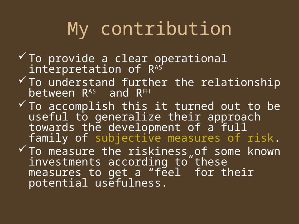
• To provide a clear operational interpretation of RAS

• To understand further the relationship between RAS and RFH

• To accomplish this it turned out to be useful to generalize their approach towards the development of a full family of subjective measures of risk.

• To measure the riskiness of some known investments according to these measures to get a “feel” for their potential usefulness.

Example

• You are offered an investment g where you win $120 with probability ½ and you lose $100 with probability ½.– g is a favorable investment: it’s expected

value is $10.– Should you accept it?

• Better yet, what is the risk in accepting g?

Traditional approach

• Use a statistical measure of dispersion to measure risk – Standard deviation– Variance– Mean absolute deviation (E|g-Eg|)– Interquartile range

• These indices measure only dispersion, taking little account of the gamble’s actual values

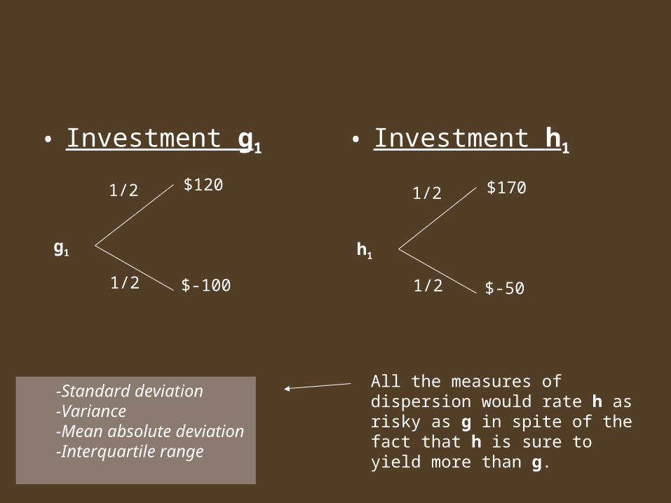
• Investment g1 • Investment h1

All the measures of dispersion would rate h as risky as g in spite of the fact that h is sure to yield more than g.

-Standard deviation-Variance-Mean absolute deviation -Interquartile range

1/2

1/2

$120

$-100

g1

1/2

1/2

$170

$-50

h1

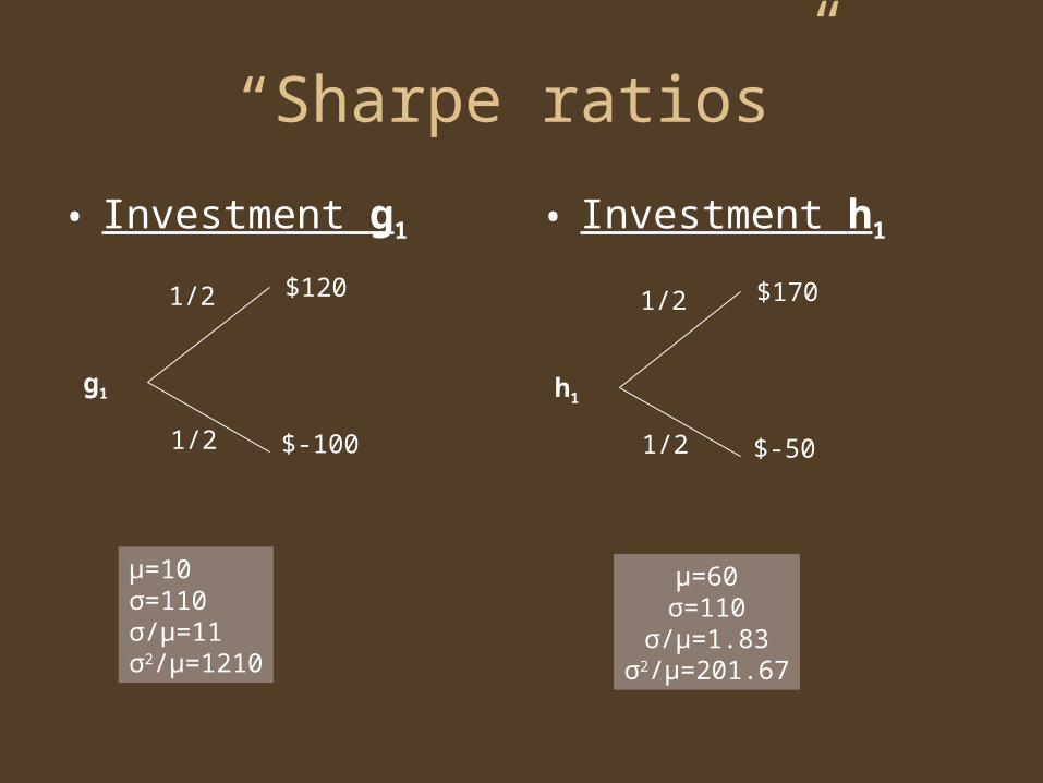
“Sharpe ratios”

• Investment g1 • Investment h1

1/2

1/2

$120

$-100

1/2

1/2

$170

$-50

μ=60σ=110

σ/μ=1.83σ2/μ=201.67

μ=10σ=110σ/μ=11σ2/μ=1210

g1 h1

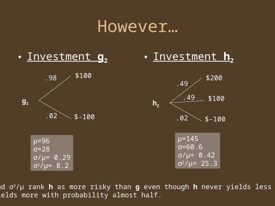
However…

• Investment g2 • Investment h2

.98

.02

$100

$-100

g2

μ=96σ=28σ/μ= 0.29σ2/μ= 8.2

.49

.02

$200

$-100

h2 $100.49

μ=145σ=60.6σ/μ= 0.42σ2/μ= 25.3

σ/μ and σ2/μ rank h as more risky than g even though h never yields less than gand yields more with probability almost half.

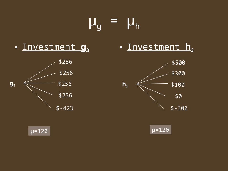
μg = μh

• Investment g3 • Investment h3

μ=120 μ=120

$100

$-300

h3

$0

$300

$500

$256

$-423

g3

$256

$256

$256

σg = σh

• Investment g3 • Investment h3

$100

$-300

h3

μ=120σ=303

μ=120σ=303

$0

$300

$500

$256

$-423

g3

$256

$256

$256

σ, σ2, E|g-Eg|, Q3-Q1, σ/μ, σ2 /μ

• All these are good measures of dispersion and normalized dispersion, but…

• Are they valid measures of risk for the purpose of decision making?

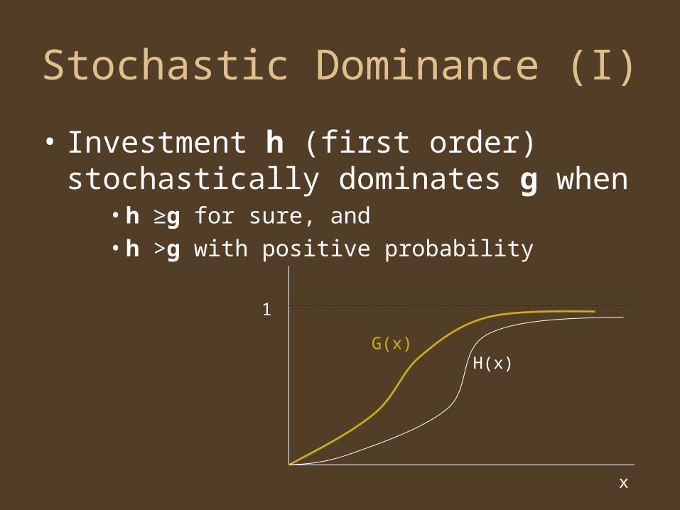
Stochastic Dominance (I)

• Investment h (first order) stochastically dominates g when

• h ≥g for sure, and• h >g with positive probability

1

x

H(x)G(x)

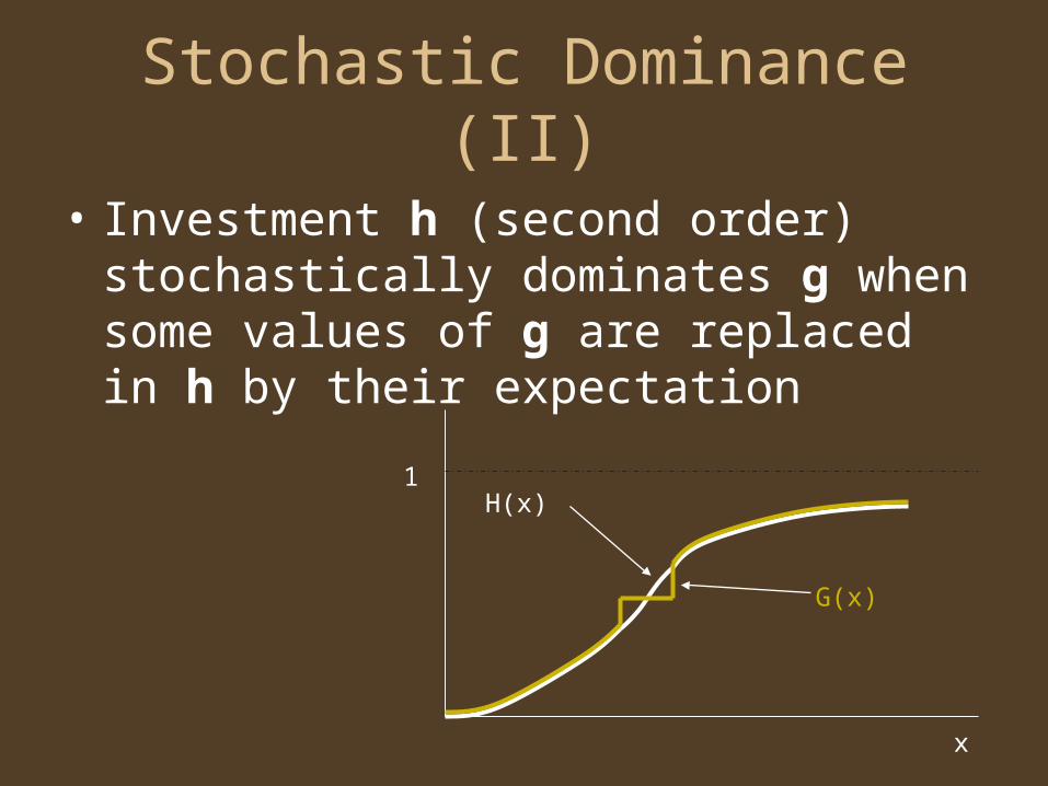
Stochastic Dominance (II)

• Investment h (second order) stochastically dominates g when some values of g are replaced in h by their expectation

1

x

H(x)

G(x)

• If we could always compare investments in terms of their stochastic dominance, we would know which investment is more risky, for the purpose of decision making:

If h stochastically dominates g then it will be preferred by any* risk averseexpected utility decision maker

Problem (I)

• Stochastic dominance is not a complete order

– One would expect any reasonable notion of riskiness to extend the stochastic dominance orders

Problem (II)

• The traditional measures all violate Stochastic Dominance

– Value at Risk also violates stochastic dominance

-Standard deviation-Variance-Mean absolute deviation -Interquartile range-Standard deviation/Mean-Variance/Mean

What to do?

Preliminaries

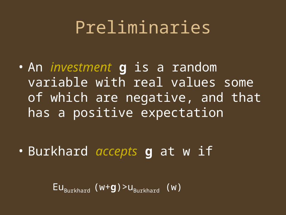
• An investment g is a random variable with real values some of which are negative, and that has a positive expectation

• Burkhard accepts g at w if

EuBurkhard (w+g)>uBurkhard (w)

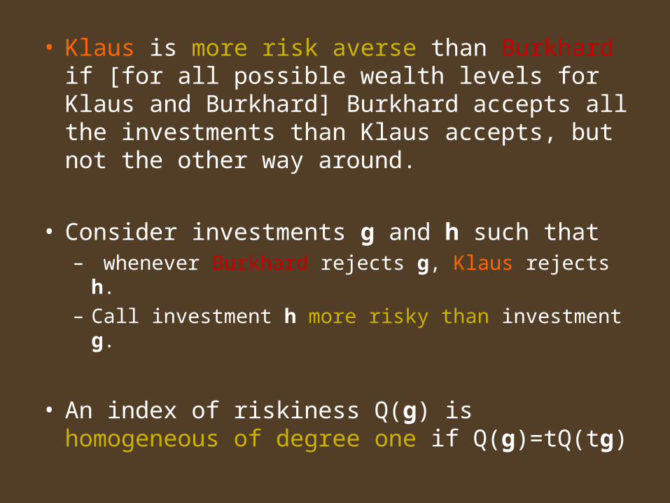
• Klaus is more risk averse than Burkhard if [for all possible wealth levels for Klaus and Burkhard] Burkhard accepts all the investments than Klaus accepts, but not the other way around.

• Consider investments g and h such that– whenever Burkhard rejects g, Klaus rejects h. – Call investment h more risky than investment g.

• An index of riskiness Q(g) is homogeneous of degree one if Q(g)=tQ(tg)

Aumann, Serrano

• Theorem (AS, 2007):For each investment g there is a unique positive number R (g) with E e-g/R(g) =1. Then,

• The index R thus defined satisfies the riskiness order and is homogeneous of degree one.

• Any index satisfying these two principles is a positive multiple of R.

Call R(g) the riskiness of g.

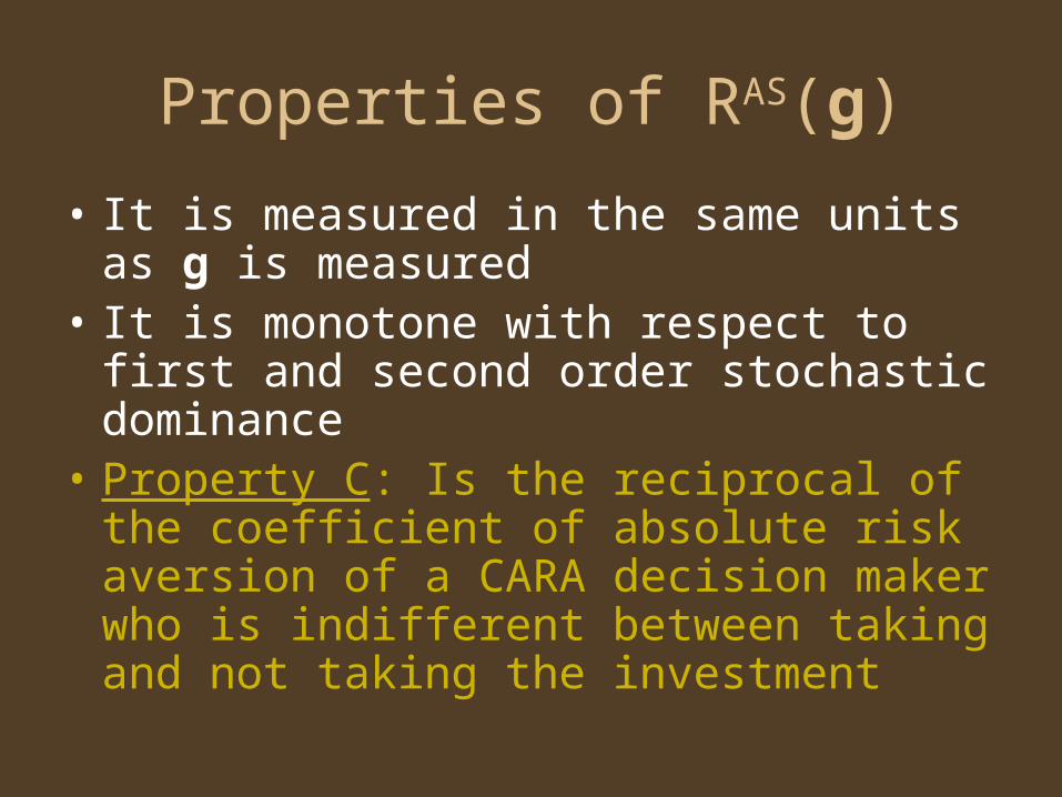
Properties of RAS(g)

• It is measured in the same units as g is measured

• It is monotone with respect to first and second order stochastic dominance

• Property C: Is the reciprocal of the coefficient of absolute risk aversion of a CARA decision maker who is indifferent between taking and not taking the investment

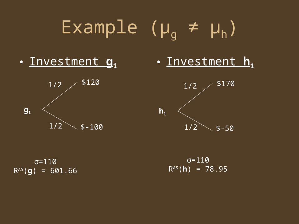
Example (μg ≠ μh)

• Investment h1• Investment g1

1/2

1/2

$120

$-100

g1

σ=110RAS(g) = 601.66

1/2

1/2

$170

$-50

h1

σ=110RAS(h) = 78.95

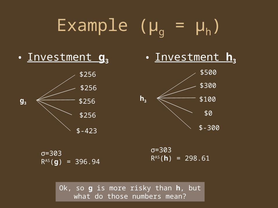
Example (μg = μh)

• Investment g3 • Investment h3

$100

$-300

h3

σ=303RAS(h) = 298.61

$0

$300

$500

Ok, so g is more risky than h, but what do those numbers mean?

σ=303RAS(g) = 396.94

$256

$-423

g3

$256

$256

$256

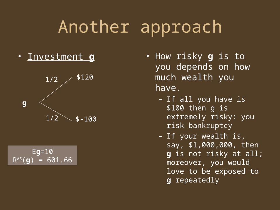
Another approach

• How risky g is to you depends on how much wealth you have.– If all you have is $100 then

g is extremely risky: you risk bankruptcy

– If your wealth is, say, $1,000,000, then g is not risky at all; moreover, you would love to be exposed to g repeatedly

• Investment g

1/2

1/2

$120

$-100

g

Eg=10RAS(g) = 601.66

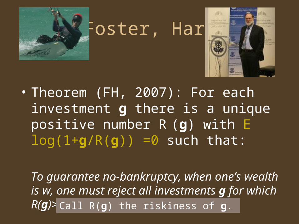
Foster, Hart

• Theorem (FH, 2007): For each investment g there is a unique positive number R (g) with E log(1+g/R(g)) =0 such that:

To guarantee no-bankruptcy, when one’s wealth is w, one must reject all investments g for which R(g)>w.

Call R(g) the riskiness of g.

Example

• If your wealth is more than $600 repeated exposure to g would (almost

surely) make you arbitrarilywealthy.

• If your wealth is less than $600 repeated exposure to g would bankrupt you with probability one.

1/2

1/2

$120

$-100

g

Eg=10RAS(g) = 601.66

RFH(g)=600

•Investment g

Properties of RFH(g)

• It is measured in the same units as g is measured

• It is monotone with respect to first and second order stochastic dominance

• Property C: Is the reciprocal of the coefficient of absolute risk aversion of a CRRA decision maker with relative risk aversion coefficient of one and who is indifferent between taking and not taking the investment

• It has a clear operational interpretation

Question

• Can we come up with an operational interpretation of RAS?

I pondered about this as I walked the shores of the State Park near my house…

me

My house

…I started thinking about subjective measures of riskiness

Objective vs. Subjective

• Both the AS and the FH approach are meant to be “objective” measures of riskiness

• Yet they relate, respectively, to CARA and CRRA preferences in a particular way

• …Use Property C to develop a definition of the riskiness of an investment for a specific decision maker

My approach• risk tolerance= (absolute risk aversion)-1

• Ri(w)=-ui’(w)/ui’’(w)

This paper: use R to define the riskiness of g

Example (CARA)

P[g<CE-2R] < e-2≈14%

• Zambrano (2008, ET): given CE, R contains information about the riskiness of g

• “CE is to µ as R is to σ”

• Definition: For any investment g “find” the wealth w(g) that makes the decision maker with utility function ui indifferent between accepting and not accepting g:

Eui (w(g)+g)≡ui(w(g))

Call Ri(w(g)) the riskiness of g for i.

The “Riwi” of g

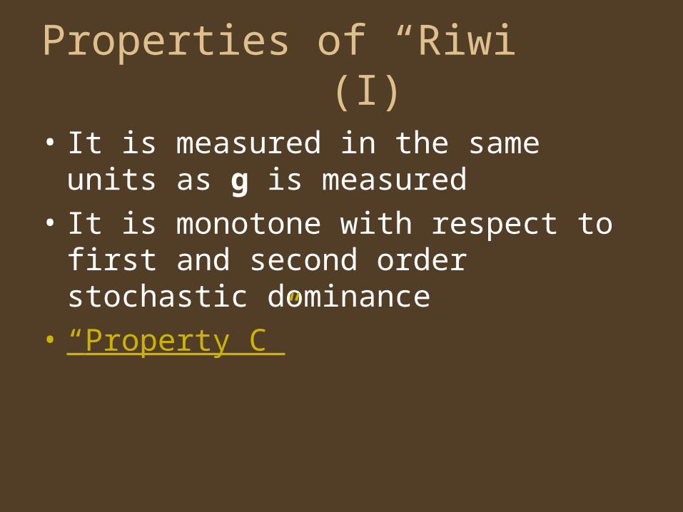
Properties of “Riwi” (I)

• It is measured in the same units as g is measured

• It is monotone with respect to first and second order stochastic dominance

• “Property C”

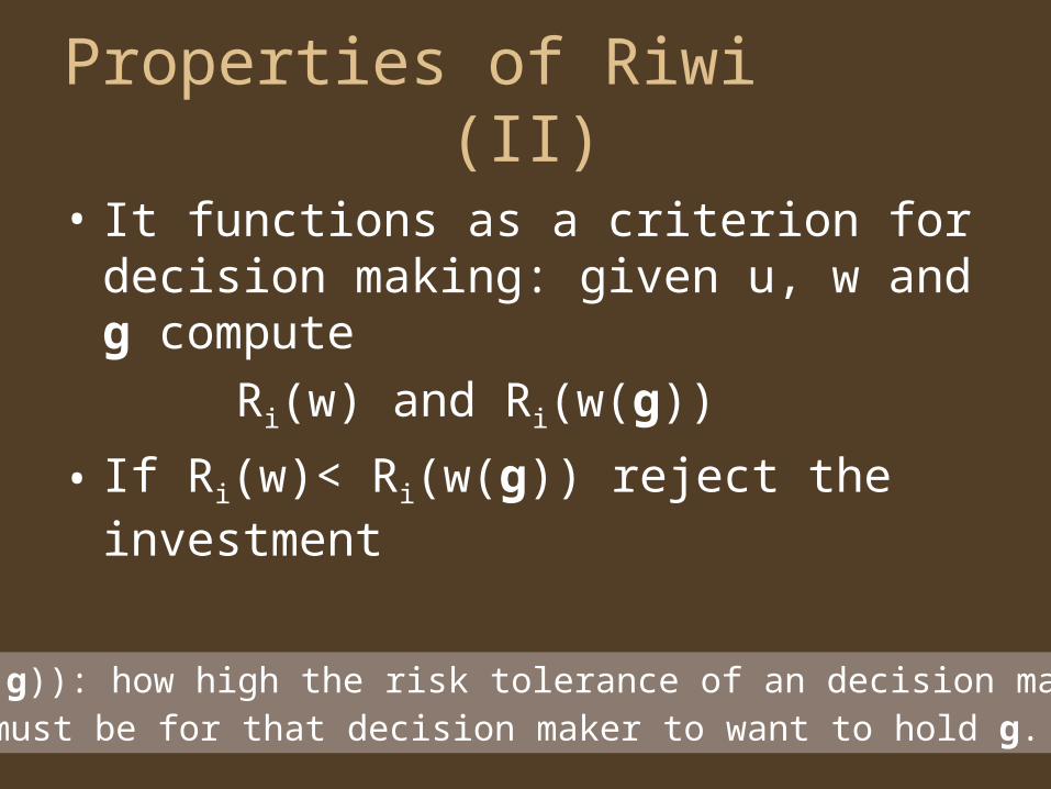
Properties of Riwi (II)

• It functions as a criterion for decision making: given u, w and g compute

Ri(w) and Ri(w(g))

• If Ri(w)< Ri(w(g)) reject the investment

Ri(w(g)): how high the risk tolerance of an decision maker must be for that decision maker to want to hold g.

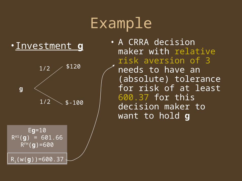
Example• A CRRA decision maker

with relative risk aversion of 3 needs to have an (absolute) tolerance for risk of at least 600.37 for this decision maker to want to hold g

1/2

1/2

$120

$-100

g

Eg=10RAS(g) = 601.66

RFH(g)=600

Ri(w(g))=600.37

•Investment g

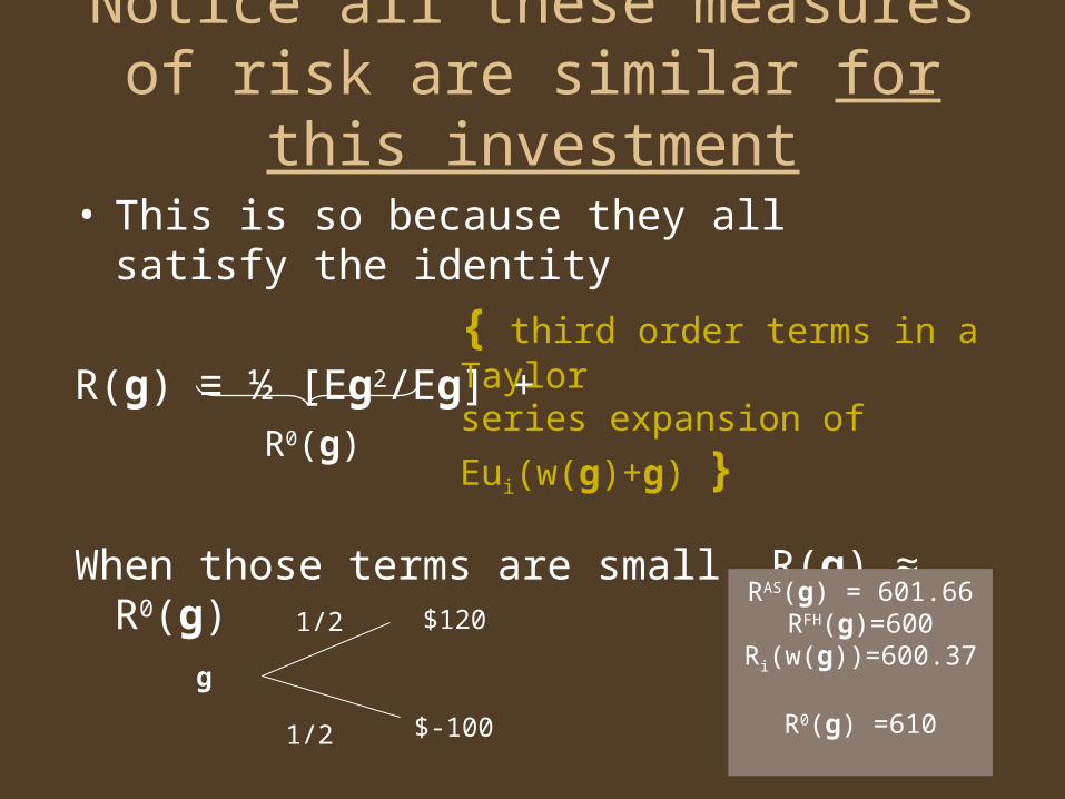
Notice all these measures of risk are similar for this investment

• This is so because they all satisfy the identity

R(g) ≡ ½ [Eg2/Eg] +

When those terms are small, R(g) ≈ R0(g)

RAS(g) = 601.66RFH(g)=600

Ri(w(g))=600.37

R0(g) =610

{ third order terms in a Taylor

series expansion of Eui(w(g)+g) }

1/2

1/2

$120

$-100

g

R0(g)

Properties of Riwi (III)

• Imagine that σ(g) shares on the investment g are offered at some price p

• How many such shares of g will a risk averse decision maker want?

• The answer to this problem is x(p), the demand function for shares of g.

Max Eu(w+x(g/σ-p)) x

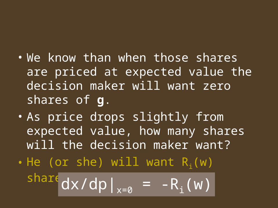
• We know than when those shares are priced at expected value the decision maker will want zero shares of g.

• As price drops slightly from expected value, how many shares will the decision maker want?

• He (or she) will want Ri(w) shares.

dx/dp|x=0 = -Ri(w)

• Ri(w) = the slope (at the origin) of the normalized demand function for shares of g for individual i and wealth w.

• Ri(w) = how much exposure to g you would want at the margin if g wasn’t priced exactly at fair value

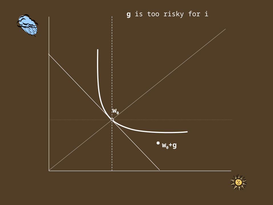
w0

w0+g

g is too risky for i

w1

w1 +g

g is not too risky for i

w(g)

w(g) +g

g is “just right” for i

An operational interpretation of Ri(w(g))

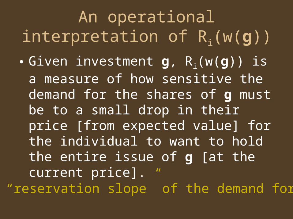
• Given investment g, Ri(w(g)) is a measure of how sensitive the demand for the shares of g must be to a small drop in their price [from expected value] for the individual to want to hold the entire issue of g [at the current price].

The “reservation slope” of the demand for g

Decision making, again

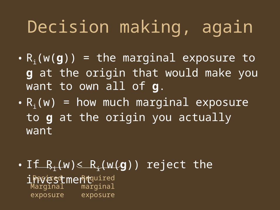
• Ri(w(g)) = the marginal exposure to g at the origin that would make you want to own all of g.

• Ri(w) = how much marginal exposure to g at the origin you actually want

• If Ri(w)< Ri(w(g)) reject the investmentDesiredMarginalexposure

Requiredmarginalexposure

An investmentRm -Rf

E 8.47

Stdev 20.42

RAS 25.50

RFH 44.82

RiWi(3) 27.83

An investmentRm -Rf

E 8.47

Stdev 20.42

RAS 25.50

RFH 44.82

RiWi(3) 27.83

A CRRA(3) decision maker with wealth $100,000 has Ri(w)=33,333

Scaling upRm -Rf 1000*(Rm –Rf)

E 8.47 8471

Stdev 20.42 20424

RAS 25.50 25500

RFH 44.82 44820

RiWi(3) 27.83 27833

A CRRA(3) decision maker with wealth $100,000 has Ri(w)=33,333

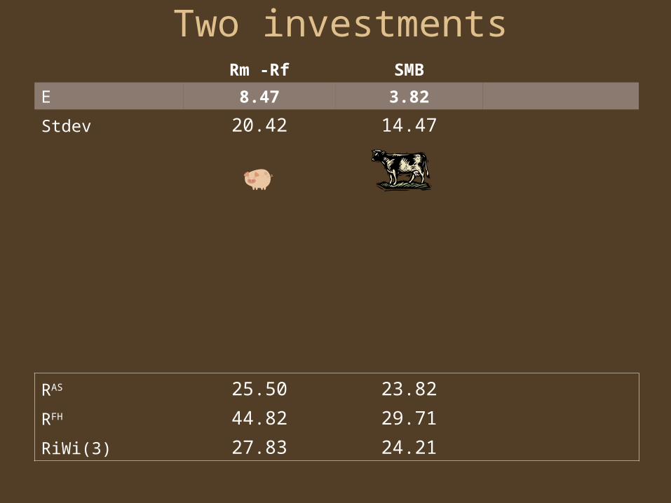
Two investmentsRm -Rf SMB

E 8.47 3.82

Stdev 20.42 14.47

RAS 25.50 23.82

RFH 44.82 29.71

RiWi(3) 27.83 24.21

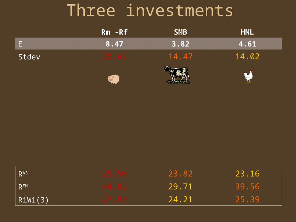
Three investmentsRm -Rf SMB HML

E 8.47 3.82 4.61

Stdev 20.42 14.47 14.02

RAS 25.50 23.82 23.16

RFH 44.82 29.71 39.56

RiWi(3) 27.83 24.21 25.39

My contribution

To provide a clear operational interpretation of RAS

To understand further the relationship between RAS and RFH

To accomplish this it turned out to be useful to generalize their approach towards the development of a full family of subjective measures of risk.

To measure the riskiness of some known investments according to these measures to get a “feel” for their potential usefulness.

Thank you for coming!

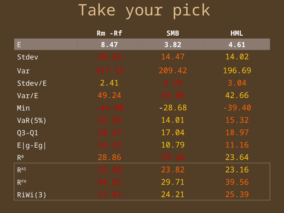
Take your pickRm -Rf SMB HML

E 8.47 3.82 4.61

Stdev 20.42 14.47 14.02

Var 417.15 209.42 196.69

Stdev/E 2.41 3.79 3.04

Var/E 49.24 54.86 42.66

Min -44.80 -28.68 -39.40

VaR(5%) 24.99 14.01 15.32

Q3-Q1 28.27 17.04 18.97

E|g-Eg| 16.22 10.79 11.16

R0 28.86 29.34 23.64

RAS 25.50 23.82 23.16

RFH 44.82 29.71 39.56

RiWi(3) 27.83 24.21 25.39