subjective comparison of wideband earpiece integations in …lib.tkk.fi/dipl/2010/urn100184.pdf ·...
TRANSCRIPT

AALTO UNIVERSITY
School of Science and Technology
Faculty of Electronics, Communications and Automation
Samppa Hyrkäs
COMPARISON OF WIDEBAND EARPIECE INTEGRATIONS IN
MOBILE PHONE
Thesis for Master of Science degree has been submitted for approval on January 4th
2010 in Espoo, Finland
Supervisor
Paavo Alku, Prof.
Instructor
Panu Nevala, MSc.

i
AALTO UNIVERSITY SCHOOL OF SCIENCE AND TECHNOLOGY
Abstract of the Master’s Thesis
Author: Samppa Hyrkäs
Name of the thesis: Comparison of Wideband Earpiece Integrations in Mobile
Phone
Date: 04.01.2010 Number of pages: 7 + 69
Department: Department of Signal Processing and Acoustics
Professorship: S-89, Acoustics and Audio Signal Processing
Supervisor: Professor Paavo Alku
Instructor: M.Sc.(Tech) Panu Nevala
The speech in telecommunication networks has been traditionally narrowband
ranging from 300 Hz to 3400 Hz. It can be expected that wideband speech call
services will increase their foothold in the markets during the coming years.
In this thesis speech coding basics with adaptive multirate wideband (AMR-WB)
are introduced. The wideband codec widens the speech band to new range from 50
Hz to 7000 Hz using 16 kHz sampling frequency. In practice the wider band means
improvements to speech intelligibility and makes it more natural and comfortable to
listen to.
The main focus of this thesis work is to compare two different wideband earpiece
integrations. The question is how much the end-user will benefit from using a larger
earpiece in a mobile phone? To find out speaker performance, objective
measurements in free field were done for the earpiece modules. Measurements were
performed also for the phone on head and torso simulator (HATS) by wiring the
earpieces directly to a power amplifier and with over the air on GSM and WCDMA
networks. The results of objective measurements showed differences between the
earpiece integrations especially on low frequencies in frequency response and
distortion.
Finally the subjective listening test is done for comparison to see if the end-user
notices the difference between smaller and larger earpiece integrations using
narrowband and wideband speech samples. Based on these subjective test results it
can be said that the user can differentiate between two different integrations and that
a male speaker benefits more from a larger earpiece than a female speaker.
Keywords: AMR-WB, wideband speech, earpiece, subjective testing, acoustic
measurements
ii
AALTO-YLIOPISTON TEKNILLINEN KORKEAKOULU Diplomityön tiivistelmä
Tekijä: Samppa Hyrkäs
Työn nimi: Laajakaistaisten matkapuhelinkuulokkeiden integroinnin vertailu
Päivämäärä: 04.01.2010 Sivumäärä: 7 + 69
Laitos: Signaalinkäsittelyn ja akustiikan laitos
Professuuri: S-89, Akustiikka ja äänenkäsittelytekniikka
Työn valvoja: Professori Paavo Alku
Työn ohjaaja: Diplomi-insinööri Panu Nevala
Perinteisesti puhelinverkoissa välitettävä puhe on ollut kapeakaistaista, kaistan
ollessa 300 - 3400 Hz. Voidaan kuitenkin olettaa, että laajakaistaiset puhepalvelut
tulevat saamaan markkinoilla enemmän jalansijaa tulevina vuosina.
Tässä lopputyössä esitellään puheenkoodauksen perusteet laajakaistaisen
adaptiivisen moninopeuspuhekoodekin (AMR-WB) kanssa. Laajakaistainen
puhekoodekki laajentaa puhekaistan 50-7000 Hz käyttäen 16 kHz näytetaajuutta.
Käytännössä laajempi kaista tarkoittaa parannuksia puheen ymmärrettävyyteen ja
tekee siitä luonnollisemman ja mukavamman kuuloista.
Tämän lopputyön päätavoite on vertailla kahden eri laajakaistaisen
matkapuhelinkuulokkeen integrointia. Kysymys kuuluu, kuinka paljon käyttäjä
hyötyy isommasta kuulokkeesta matkapuhelimessa? Kuulokkeiden suorituskyvyn
selvittämiseksi niille tehtiin objektiivisia mittauksia vapaakentässä. Mittauksia
tehtiin myös puhelimelle pää- ja torsosimulaattorissa (HATS) johdottamalla kuuloke
suoraan vahvistimelle, sekä lisäksi puhelun ollessa aktiivisena GSM ja WCDMA
verkoissa. Objektiiviset mittaukset osoittivat kahden eri integroinnin väliset erot
kuulokkeiden taajuusvasteessa ja särössä erityisesti matalilla taajuuksilla.
Lopuksi tehtiin kuuntelukoe tarkoituksena selvittää erottaako loppukäyttäjä
pienemmän ja isomman kuulokkeen välistä eroa käyttäen kapeakaistaisia ja
laajakaistaisia puhelinääninäytteitä. Kuuntelukokeen tuloksien pohjalta voidaan
sanoa, että käyttäjä erottaa kahden eri integroinnin erot ja miespuhuja hyötyy
naispuhujaa enemmän isommasta kuulokkeesta laajakaistaisella puhekoodekilla.
Hakusanat: AMR-WB, laajakaistainen puhe, kuuloke, subjektiivinen testaus,
akustiset mittaukset

iii
Preface
This thesis has been made for Nokia Corporation Smart phones Electro Mechanics
Audio Oulu unit during November 2008 – December 2009. I’d like to thank all my
colleagues at Nokia, especially my instructor Panu Nevala who guided my through this
whole process. I would also like to thank my supervisor, professor Paavo Alku.
Thanks to Kalle Mäkinen and Henri Toukomaa for providing information about
subjective testing. I appreciate Lauri Veko for allowing me to use his earpiece
measurement data in this thesis. Lauri Leviäkangas vitally helped me with laboratory
equipment. Toni Soininen aided me with many acoustic related questions. I also want to
send warm thanks to Nokia Smart phones EM audio team for the friendly atmosphere
that was created there.
Finally, I would like to thank my family for their patient support and encouragement
during my studies and the process of writing this thesis. Special thanks to my girlfriend
Hannariikka for her love and patience during the writing period.
Thank you!
Oulu 04.01.2010
Samppa Hyrkäs

iv
Contents
Abstract.........................................................................................................................i
Tiivistelmä....................................................................................................................ii
Preface.........................................................................................................................iii
Contents.......................................................................................................................iv
Abbreviations...............................................................................................................v
1. Introduction ............................................................................................. 1
2. Background theory of speech and hearing ................................................. 2
2.1 Speech properties ................................................................................. 2
2.1.1 Speech production ......................................................................... 2
2.1.2 Hearing of speech .......................................................................... 4
3. Fundamentals of gsm coders ..................................................................... 6
3.1 Speech coding basics ............................................................................ 6
3.1.1 Waveform coders ........................................................................... 6
3.1.2 Source coders ................................................................................ 7
3.1.3 Present speech codecs .................................................................... 7
3.2 Linear prediction in speech coding ......................................................... 8
3.2.1 Basics of linear prediction .............................................................. 8
3.2.2 Short term prediction ..................................................................... 9
3.2.3 Long term prediction ...................................................................... 9
3.2.4 Optimization of prediction filter ...................................................... 9
3.2.5 Windowing and autocorrelation method ......................................... 10
3.2.6 LPC-synthesis ............................................................................. 12
3.2.7 Code-Excited Linear Prediction (CELP) speech coding ................... 12
4. Adaptive Multi-Rate Wideband codec AMR-WB .................................... 15
4.1 History and standardization ................................................................. 15
4.2 General description of AMR-WB ......................................................... 15
4.3 Encoder ............................................................................................. 17
4.4 Decoder ............................................................................................. 19
5. Mobile phone acoustics ........................................................................... 21
5.1 Audio path from mobile phone’s antenna to speaker .............................. 21
5.2 Audio module in mobile phones ........................................................... 23
5.2.1 Dynamic loudspeaker ................................................................... 23
5.2.2 Leak types, front and back cavity ................................................... 25
5.2.3 Loudspeaker implementation in different phone models ................... 27
6. Objective measurements ......................................................................... 29
6.1 Theory of audio measurements ............................................................ 29
6.1.1 Transfer function ......................................................................... 29
6.1.2 Frequency response ..................................................................... 30
6.1.3 Distortion ................................................................................... 31
6.2 Earpiece measurements in free field ..................................................... 31
6.2.1 Earpiece measurement procedure and equipment ............................ 31
6.2.2 Results of earpiece measurements .................................................. 32

v
6.3 Measurement for wired earpieces integrated to Nokia mobile phone ........ 34
6.3.1 Selection criteria's for phones in the test ........................................ 34
6.3.2 Measurement equipment and procedure for wired earpieces ............ 34
6.3.3 Results of the wired earpiece measurements on HATS ..................... 36
6.4 Nokia mobile phone measurements over the air ..................................... 38
6.4.1 Information about the phones in the test ......................................... 38
6.4.2 Measurement equipment and procedure ......................................... 39
6.4.3 Measurement results .................................................................... 40
6.5 Discussions about the objective measurements ...................................... 43
7. Subjective test on two earpiece integrations ............................................. 44
7.1 Overview of subjective testing ............................................................. 44
7.1.1 Test type and listener selection ...................................................... 44
7.2 Creation of test material ...................................................................... 46
7.2.1 Full band files and selecting test samples ....................................... 47
7.2.2 Lowpass filtering to 7.8 kHz .......................................................... 47
7.2.3 Call recording with HATS............................................................. 48
7.2.4 Loudness balancing ..................................................................... 49
7.2.5 Lowpass filtering, wideband 7.8 kHz, narrowband 5.7 kHz .............. 50
7.2.6 Downsampling from 48 kHz to 24 kHz ........................................... 50
7.2.7 HATS ear canal (DRP-ERP) filter ................................................. 50
7.2.8 Upsampling from 24 kHz to 48 kHz ................................................ 52
7.2.9 Noise removal ............................................................................. 52
7.2.10 Discussion of the listening test files ................................................ 52
7.3 Listening test set-up ............................................................................ 53
7.3.1 Briefing for the listener ................................................................ 54
7.3.2 User interface .............................................................................. 55
7.4 Results of the subjective test ................................................................ 55
7.4.1 How the data is analyzed .............................................................. 55
7.4.2 Analysis of the results ................................................................... 56
7.5 Discussions about the subjective test .................................................... 58
8. Conclusions ............................................................................................ 59
9. References .............................................................................................. 60
10. Appendices ............................................................................................. 63
Appendix A: Large speaker used in Nokia 6720c mobile phone ........................... 63
Appendix B: Small speaker used in Nokia 6220c mobile phone ........................... 64
Appendix C: Listening test instructions (in Finnish) ........................................... 65
Appendix D: Matlab code for 7.8 khz filter ....................................................... 66
Appendix E: Matlab code for 5.5 khz lowpass filter ........................................... 67
Appendix F: Type 4606 hats position table for Nokia 6720c ......................... 68
Appendix G: Type 4606 hats position table for Nokia 6220c ........................ 69

vi
Abbreviations
3G International Mobile Telecommunications-2000 (IMT-2000)
3GPP 3rd
Generation Partnership Project
ACELP Algebraic Code-Excited Linear Prediction
AGC Adaptive Gain Control
AMR Adaptive Multi-Rate speech codec
AMR-NB Adaptive Multi-Rate NarrowBand speech codec
AMR-WB Adaptive Multi-Rate WideBand speech codec
A/D Analog-to-Digital (conversion)
B&K Brüel & Kjaer
CI95% 95% Confidence Interval
CELP Code-Excited Linear Prediction
CMOS Comparative Mean Opinion Score
dB deciBel
D/A Digital-to-Analog
DCT Discrete Cosine Transform
DM Delta Modulation
DRC Dynamic Range Controller
DRP Ear-Drum Reference Point
DUT Device Under Test
EFR Enhanced Full Rate speech codec
ERP Ear Reference Point
ETSI European Telecommunications Standards Institute
FIR Finite Impulse Response
FR Full Rate speech codec
FS Full Scale
Glottis The space between the vocal cords
GSM Global systems for mobile communications
HATS Head And Torso Simulator
IEC International Electrotechnical Commission
IHF Integrated Hands-Free
ISP Immittance Spectral Pair
LP Linear Predicting
LPC Linear Predictive Coding
LTP Long Term Prediction
MDRC Multiband Dynamic Range Controller
MIPS Millions of Instructions Per Second
MOS Mean Opinion Score
PCM Pulse Code Modulation
RF Radio Frequency
RPE-LTP Regular Pulse Excitation with Long Term Prediction
SNR Signal-to-Noise Ratio
THD Total Harmonic Distortion
THD+N Total Harmonic Distortion and Noise
Vocoder VOice CODER
VSELP Vector Sum Excited Linear Prediction
WCDMA Wideband Code Division Multiple Ac

1
1. INTRODUCTION
In telecommunication speech transmission is based nowadays on digital transmission.
When speaking into the phone's microphone the human speech is in analogical form.
The microphone transforms the air pressure variations to a digital form with an analog-
to-digital (AD) converter and after that the speech is digital sampled data. The
traditional telephone system uses a pulse code modulation (PCM) method to do this AD
conversion. The bit rate of PCM requires bandwidth too much for cellular radio
transmission and, therefore, the speech information has to be compressed. This
compression is also called speech coding.
The aim of speech coding in transmission systems is to optimize the speech quality in
relation to consumed bits and error robustness. There are many different speech coding
methods. The best coding methods compress the data so that the human ear does not
sense much difference to the uncompressed version of the speech. From the speech
codecs standardized for the cellular telephony, adaptive multi-rate wideband speech
codec (AMR-WB) produces the most natural sound.
The traditional land line and the global systems for mobile communications (GSM)
network have used the speech bandwidth 300Hz-3400Hz. The first commercial network
with speech coding method AMR-WB on the bandwidth 50-7000Hz was opened in
Moldova at September 2009 [24]. The AMR-WB is widely expected to become a new
standard for mobile voice communications. It can be expected that operators will
introduce the AMR-WB voice service in many networks around the world in the near
future.
This thesis focuses on comparing two different earpiece integrations in wideband and
narrowband speech calls. The idea is to find out how much a user benefits if a larger
earpiece is used in AMR-WB calls and in AMR-NB calls for comparison.
This paper contains information about hearing and speech, current speech coding
methods on the market with the upcoming AMR-WB codec. A wideband audio path
from the antenna to the loudspeaker is introduced. The loudspeaker enclosures affect on
the overall acoustics and different cavities with leaks is presented.
The objective measurements are done to find out if there is any significant difference
between the earpieces in free field without the phone, on the head and torso simulator
(HATS) by using a connection directly from the measurement equipment to the speaker
on the phone. Also, the phones' audio performances are measured during the call to
evaluate the performance under the whole audio path. The subjective test is done in
Oulu Nokia Teknologiakylä site to get information how users sense the difference
between the two phones. Finally the objective results are compared with subjective test
results, which heavily support the decision taken.
2
2. BACKGROUND THEORY OF SPEECH AND HEARING
This chapter introduces the speech properties and coding used in mobile communication
systems.
2.1 Speech properties
Speech is an excellent way to communicate with other people. Visual effects can be
used to make the speech more effective, but in telephone calls the voice is the only
available way to communicate.
Humans have unique characteristics compared to other living creatures on earth: speech.
It is in everyday usage and self-evident for us, but if something goes wrong then we
notice how much it means to us.
The speech is acoustic sound waves from the speaker’s vocal organs to the listener’s
ears. The smallest posited structural unit of the speech is a phoneme [1]. For example,
in the Finnish language there are 24 phonemes. The understandable words are made
from phonemes after another and sentences are formed by placing pauses between the
sequential phonemes.
Phonemes can be divided into two groups: voiced and unvoiced phonemes. In the
Finnish language, the vocal phonemes and some of the consonants (e.g. n, m, j and v)
are voiced. The parts of the consonants are unvoiced (e.g. k, p, t, f, s and h). The
unvoiced phonemes are noisy without periodicity. The voiced parts are periodic in the
time-domain and harmonic structure in the frequency-domain. These properties are
from vocal tract resonances. There are peaks in the voiced phoneme spectrum and those
are vocal tract resonance frequencies called formants. The different phonemes can be
distinguished by looking at the formant structure. Finnish vocal phonemes can be
differentiated with the first two lowest formants. It is, however desirable that there are
higher formants included when transmitting a speech signal.
2.1.1 Speech production
The speech is produced from a filtering operation, where the stimulus goes through
about a 17 cm long sound channel (see Figure 1) formed by larynx, pharynx, oral and
nasal cavity [2]. The sound channel is a physiological filter, which shapes the stimulus
from the lungs. Different sounds are formed by changing the filtering characteristics.
These properties change when the profile of the sound channel is shaped with the
different position of, for example tongue and lips.

3
Figure 1: The human vocal organs [3].
Voiced sound forming starts from the lungs. Midriff muscle press’ the lungs and causes
overpressure to the trached. The vocal cords start to vibrate because the air flows from
the lungs through a small hole between the vocal cords called the glottis. The vibrating
frequency is called the fundamental frequency, which is about 100 – 110 Hz for males
and 200 Hz for females. The periodic airflow pulse from the vocal cords is called the
glottis stimulus. In the end of the sound channel, the filtered glottis stimulus diverges
from the mouth and changes to audible pressure wave.
One difference between the voiced and unvoiced sound is that voiced sounds have
greater amplitude than unvoiced. The waveforms of voiced sounds are exact periodic,
which is very important from the speech coding point of view. Instead of using the
glottis stimulus in the unvoiced sounds, they are formed in narrow or closed parts of the
sound channel. Unvoiced sounds are often similar to random noise and the glottis
stimulus is not used at all.
One way to present the speech production is to use a simplified source-filter model of
speech as in Figure 2. This kind of model can be also used in the formant synthesis to
produce synthetic speech. Voiced sounds are produced from the glottis stimulus and
unvoiced from noise. Both voiced and unvoiced stimulus are connected to a binary
switch. After the switch there is an input for a linear filter, which represents other parts
of the speech production, especially the sound channel [4]. Gain 𝐴0 is needed for
balancing the speech signal energy on every stimulus and filter combination. The 𝐹0in
Figure 2 is the fundamental frequency of voiced sounds.

4
Figure 2: Source-filter model of speech [1].
2.1.2 Hearing of speech
The role of the ear is to receive the sound wave from the air and guide it to the hearing
nervous system. The sensitivity of the human ear is not always so good compared to an
animal ear, but it has a unique special assignment and ability: speech analysis and
recognition. The structure of the human ear can be seen in Figure 3.
The human ear is usually divided into three parts: inner, middle and outer ear. The
auditory canal ends to the tympanic membrane in the outer ear. Inside the eardrum in
the middle ear is three bones connected to each other: The hammer, anvil and stirrup.
These bones transmit and strengthen the sound, but also prevent the wide eardrum
movement effect to the inner ear. The purpose of the middle ear is to adjust the
impedances between the air in the outer ear and the liquid in the inner ear. The three
bones mentioned above act as a mechanical impedance converter by transferring low
pressure and high particle speed (in air) into high pressure and low particle speed (in
liquid) [1].
The speech recognizing and understanding starts in the inner ear. The cochlea is a very
sensitive organ, which analyzes the sound and transforms the sound to nerve impulses.
The semicircular canals are not for hearing, but for human balance.

5
Figure 3: The structure of human ear [7].

6
3. FUNDAMENTALS OF GSM CODERS
3.1 Speech coding basics
The idea of speech coding is to compress the original sound data as much as possible
without losing the quality too much [4]. This compression enables the speech
transmission with smaller resources and increases the amount of information to be
transmitted with limited resources.
When comparing audio formats, the sound sources have to be selected carefully. The
normal audio CD has a very good audio quality and to the present day it has been the
standard physical medium for sale of commercial audio recordings. If the CD audio is
transmitted with stereo sound, it takes over 1.4 Mbits/s transfer speed. The bandwidth in
CD is half from the sampling rate 44.1 kHz/2 = 22 kHz. In a traditional telephone
system, the used bit rate is 64 kbits/s, which is about 1/22 of CD audio data rate called
PCM. Usually the CD audio quality is compared to all audio formats, where the PCM is
used to grade speech audio quality.
Before the analog speech is coded to PCM format some signal processing must be done.
First the original speech signal is filtered and the unwanted signal components are
removed. The traditional telephone network uses a bandwidth between 300 Hz – 3400
Hz so the frequencies outside the band are filtered away. After filtering the speech
signal is then sampled. This means taking samples of the signal at the sampling
frequency, which is in the PCM case 8 kHz. When sampling is done, the signal values
are transformed to discrete numerical values or quantized. The quantization is done with
13 or 14 bits in telephone networks. Finally, after the quantization the signal is coded.
Signal coding reduces the bits needed for data transmission for instance compressing
with A- or µ-law decreases the sample to 8 bit with a very small signal quality loss. The
basic principle of speech coding is shown in Figure 4.
Figure 4: Speech coding principle from original sound to coded signal.
Speech coding methods are divided into two groups: waveform coders and source
coders. The waveform coders try to transmit the original signal to the destination and
keep the same waveform. The idea of source coders is to model the mechanism how the
waveform is produced by parameters. There are also hybrid coding methods that
connect both of these methods.
3.1.1 Waveform coders
Most of the sounds that we hear are vibrations through air. These vibrations can be
transformed into electrical signals with the help of the microphone. The microphone
signal is then coded on the desired media. Waveform coders try to preserve the
electrical signal waveform as much as possible.

7
The advantage of the waveform coders is that they can be applied to different kinds of
signals like music, signaling or data transfer. If there is noise added to the signal,
waveform coders maintain their performance.
The simplest waveform coding method is pulse-code modulation PCM. It is
standardized in ITU-T G.711 [5]. PCM transforms the linear 13 or 14 bit samples to 8
bit one by one according to the standard. Using PCM guarantees very good speech
quality, but bit rate is fairly high.
There are several ways to improve pulse-code modulation performance. One is to use
differential modulation, which is based on prediction of the samples of the signal and
baseline of PCM. Another method is adaptive quantization, where the size of the
quantization step is varied allowing the reduction of the required bandwidth for a given
signal-to-noise ratio. These two coding methods can achieve almost as good speech
quality as PCM, but with a smaller bit rate.
There are also other waveform coding methods for example, delta modulation and
adaptive transform coding. The latter method uses fast transforming algorithms, like
discrete cosine transform DCT to cut the signal on a large amount of frequency bands.
The bit amount of frequency band multipliers is selected based on the speech spectrum.
Delta modulation is one variant of PCM, which uses a very low bit amount to indicate
the change of the previous sample.
3.1.2 Source coders
Vocoders or source coders are developed to achieve efficient speech coding. The speech
signal is sent to the transmission channel as parameters reducing the bit rate noticeably.
Even the speech is in parameter form, it can be reconstructed in the receivers end so that
the human ear senses characteristic parts of the original signal. Most of the vocorders
are based on the speech production model in Figure 2.
There are many flaws in source coders. Because the vocoders are optimized to speech
coding, other types of signals suffer more in the coding. Usually the speech quality is
worse and more synthetic than waveform coders. Vocoders are also talker dependent
and male voices are typically heard with better quality. If there is noise added to the
signal, the quality of the coded speech decreases recognizably. Most of the speech
coders used in telecommunication are based on linear prediction and its variations.
3.1.3 Present speech codecs
There are many speech codecs available for speech compressing. The most common
codecs are listed in Table 1. There are several codecs used in mobile communication for
example typically, the supported codecs in mobile phones are GSM HR, GSM FR,
GSM EFR and GSM AMR. Also AMR-WB is specified for GSM and WCDMA and the
first commercial AMR-WB network was launched to consumers on autumn 2009 [24].
In Table 1 the Mean Opinion Score, MOS means the average quality that listeners
perceive in a listening test on a scale of 1-5. Values from 4.0 to 4.5 are as good as
telephone land line, mobile networks are graded 3.5-4.0 and values 2.5-3.5 sound like
synthetic speech [8].

8
Table 1: Most common speech codecs [6]
Codec Coding method Bit rate (kbit/s) MOS Complexity MIPS AMR WB (G.722.2) ACELP 6.60 - 23.85 WB 40
G.722 SB-ADPCM 48 / 56 / 64 WB 5
G.711 PCM 64 4.4 0.5
G.726 ADPCM 16 / 24 / 32 40 2 / 3.2 / 4.0 / 4.2 2
G.727 E-ADPCM 16 / 24 / 32 40 2 / 3.2 / 4.0 / 4.2 2
AMR ACELP 4.75 - 12.2 ≤ 4.2 17
GSM EFR ACELP 12.2 4.2 16
CDG27 QCELP13 1.0 / 6.2 / 13.3 4.1
IS-127 ACELP (EVCR) 0.8 / 4 / 8.55 4.1 24
G.728 LD-CELP 16 4 30
IS-641 ACELP 7.4 4 15
G.723.1 A/MP-MLQ CELP 5.2 / 6.2 3.7 / 4.0 16
G.729 CS-ACELP 8 3.9 20
G.729a CS-ACELP 8 3.7 11
GSM FR RPE-LTP 13 3.7 5 - 6
GSM HR VSELP 5.6 3.6 14
IS-54 VSELP 7.95 3.5 14
IS-96-B QCELP 0.8 / 2 / 4 / 8.55 3.5 15
Inmarsat-Aero MPLPC 8.9 3.5
TETRA ACELP 4.56 < 3.5 15
JDC VSELP 6.7 < 3.5
Inmarsat-M IMBE 4.15 < 3.5 7
Inmarsat-P AMBE 3.6 < 3.5
DOD FS 1016 CELP 4.8 3.2 16
DOD FS prop. MELP 2.4 3.2 40
Inmarsat-B APC 9.6 / 12.8 3.1 / 3.4 10
JDC-HR PSI-CELP 3.45 < 3.0
DOD FS 1015 LPC-10 2.4 2.3 7
The complexity in Table 1 describes how many million instructions per second MIPS
are calculated. This parameter tells how much the processor requires calculation and
that way causes computational delay. The processing delay is always minimized during
the designing process.
One impact, which is not mentioned in Table 1, is memory consumption. It affects the
complexity, but it is not noted in this case. The other delays, which are not in Table 1,
are algorithm, multiplexing and transmission delay. These delays are about the same for
each speech codec used in mobile networks and for that reason are left out from Table
1.
3.2 Linear prediction in speech coding
Linear predictive coding (LPC) is one of the most powerful speech analysis techniques,
and one of the most useful methods for encoding good quality speech at a low bit rate. It
provides extremely accurate estimates of speech parameters, and is relatively efficient
for computation. Almost all present speech codecs are based on this method [4].
3.2.1 Basics of linear prediction
LPC starts with the assumption that the speech signal is produced by a buzzer at the end
of a tube. The glottis produces the buzz, which is characterized by its intensity
(loudness) and frequency (pitch). The vocal tract (the throat and mouth) forms the tube,
which is characterized by its resonances, which are called formants.
LPC analyzes the speech signal by estimating the formants, removing their effects from
the speech signal, and estimating the intensity and frequency of the remaining buzz. The

9
process of removing the formants is called inverse filtering, and the remaining signal is
called the residue.
The numbers which describe the formants and the residue can be stored or transmitted
somewhere else. LPC synthesizes the speech signal by reversing the process: use the
residue to create a source signal, use the formants to create a filter (which represents the
tube), and run the source through the filter, resulting in speech.
3.2.2 Short term prediction
In LPC analysis the sequentially placed samples’ correlation is utilized efficiently. The
signal sample value is estimated by forming a linear combination of a few previous
samples. In linear combination, these previous samples are multiplied by certain
parameters. When the multipliers and products are added up, the prediction to the
sample value is obtained. This value is subtracted from the sample value and the
prediction error, and the residue is attained as a result.
The prediction is repeated to a certain amount of sequential samples using the same
coefficient parameters. After this, the square error between the original and predicted
signal samples is minimized. The result shows the optimal coefficient parameters. The
filter is a finite impulse response (FIR) type and called the prediction filter.
3.2.3 Long term prediction
The long term prediction filter estimates the coming residual peaks at the end of the
pitch-period and removes the peaks with inverse filtering. After inverse filtering the
new residual is more like hum, which can be quantized with a small amount of bits.
The short term predictor’s prediction error signal is like an impulse, which is from the
voiced speech signal glottis pulses. Describing the impulse signal by a low amount of
data bits is problematic, which is why the long term predictor is added after short term
prediction filter.
3.2.4 Optimization of prediction filter
In general form the LPC is done at p-degrees, when samples s(n) prediction š(n)
calculation is done with p previous samples (s(n-1), s(n-2),…,s(n-p)). The coefficient
parameters are marked on a(k). The expression for prediction is obtained in (1).
š 𝑛 = 𝑎 𝑘 𝑠(𝑛 − 𝑘)𝑝𝑘=1 (1)
The prediction error called residual can be expressed as:
𝑒 𝑛 = 𝑠 𝑛 − š 𝑛 = 𝑠 𝑛 − 𝑎 𝑘 𝑠 𝑛 − 𝑘 𝑝𝑘=1 (2)
In the infinite length time window, the residual signal energy is expressed as:
𝐸 = 𝑒2 𝑛 = 𝑠 𝑛 − 𝑎 𝑘 𝑠 𝑛 − 𝑘 𝑝𝑘=1
2𝑛𝑛 (3)
= [𝑛 𝑠2 𝑛 − 2𝑠 𝑛 𝑎 𝑘 𝑠 𝑛 − 𝑘 𝑝𝑘=1
+ 𝑎 𝑘 𝑠 𝑛 − 𝑘 𝑝𝑘=1
2] (4)

10
The coefficients a(k), 1 ≤ 𝑘 ≤ 𝑝 that realize the mean square error criterion is attained
when the residual energy’s partial derivatives are set to zero with regard to a(i):
𝜕𝐸
𝜕𝑎 (𝑖)= 0, 1 ≤ 𝑖 ≤ 𝑝 (5)
−2𝑠 𝑛 𝑠 𝑛 − 𝑖 + 2 𝑎 𝑘 𝑠 𝑛 − 𝑘 𝑠(𝑛 − 𝑖)𝑝𝑘=1 𝑛 = 0 (6)
𝑠 𝑛 𝑠 𝑛 − 𝑖 = 𝑎 𝑘 𝑠 𝑛 − 𝑘 𝑠 𝑛 − 𝑖 , 1 ≤ 𝑖 ≤ 𝑝𝑝𝑘=1𝑛 (7)
The equation (7) can be expressed in the following form:
𝑎 𝑘 𝜙 𝑖, 𝑘 = 𝜙 𝑖, 0 , 1 ≤ 𝑖 ≤ 𝑝𝑝𝑘=1 , (8)
where 𝜙 𝑖, 𝑘 = 𝑠 𝑛 − 𝑖 𝑠(𝑛 − 𝑘)𝑛
The optimized prediction filter gives the residual energy:
𝐸𝑚𝑖𝑛 = 𝜙 0,0 − 𝑎 𝑘 𝜙 0, 𝑘 𝑝𝑘=1 (9)
= 𝑠2 𝑛 − 𝑎 𝑘 𝑠 𝑛 𝑠 𝑛 − 𝑘 𝑛 𝑝𝑘=1𝑛 (10)
= 𝐸𝑜𝑟𝑖𝑔 − 𝐸(𝑝) (11)
Equation (11) shows that residual energy 𝐸𝑚𝑖𝑛 can be expressed as the subtraction of
original signal 𝐸𝑜𝑟𝑖𝑔 and prediction degree dependend energy 𝐸(𝑝) [8].
3.2.5 Windowing and autocorrelation method
There are two ways to calculate LPC, the autocorrelation and covariance methods. The
autocorrelation method is most often used because it requires less calculation and the
FIR-filter is always at a minimum phase after optimization. The minimum phase filter is
necessary so that the infinite impulse response (IIR) filter decoder is stable.
In theory, the FIR-filter optimization is done in an infinite length time frame, but in
practice calculation of the speech signal is divided into short segments. The division
into segments is done by multiplying the speech signal on a window function, which is
nonzero on the time frame 0 ≤ 𝑛 ≤ 𝑁 − 1. The simplest window function is rectangle
(w(n)=1, 0 ≤ 𝑛 ≤ 𝑁 − 1), which divides the signal into N sample long segments. The
most common window functions in LPC are the Hanning and Hamming windows
described below.
Hamming: 𝑤 𝑛 = 0.54 − 0.46 cos 2𝜋𝑛
𝑁−1 , 0 ≤ 𝑛 ≤ 𝑁 − 1 (12)
Hanning: 𝑤 𝑛 =1
2 1 − cos
2𝜋𝑛
𝑁−1 , 0 ≤ 𝑛 ≤ 𝑁 − 1 (13)
If these two windowing methods (11), (12) are compared to the rectangular window the
advantage is that Hamming and Hanning decrease the unwanted transitions from the
beginning and the end of the signal frame. The shapes of Hamming and Hanning
windows are about the same; the functions gain their maximum value in the middle of
the time window and their minimum values near zero at the beginning and the end.
The windowing produces the following signal:

11
𝑠 𝑛 = 𝑠0 𝑛 𝑤(𝑛) (14)
where, 𝑠0 𝑛 is original speech signal, which is continuous and nonzero, w(n) is
windowing function, which is nonzero at time interval 0 ≤ 𝑛 ≤ 𝑁 − 1, s(n) describes
the speech signal predicted in LPC-analysis.
Now the equation (8) term ϕ can be shown as follows:
𝜙 𝑖, 𝑘 = 𝑠 𝑛 − 𝑖 𝑠 𝑛 − 𝑘 𝑁−1+𝑝𝑛=𝑜 (15)
where 1 ≤ 𝑖 ≤ 𝑝 and 1 ≤ 𝑘 ≤ 𝑝.
When n-i=j is placed to Equation (15)
𝜙 𝑖, 𝑘 = 𝑠 𝑗 𝑠 𝑗 + 𝑖 − 𝑘 𝑁−1+𝑝−𝑖𝑗=−𝑖 , (16)
where 1 ≤ 𝑖 ≤ 𝑝 and 1 ≤ 𝑘 ≤ 𝑝. s(j) is nonzero between 0 ≤ 𝑗 ≤ 𝑁 − 1 because of the
windowing and for this reason the Equation (16) can be presented as:
𝜙 𝑖, 𝑘 = 𝑠 𝑗 𝑠 𝑗 + 𝑖 − 𝑘 𝑁−1−(𝑖−𝑘)𝑗=0 , (17)
where 1 ≤ 𝑖 ≤ 𝑝 and 1 ≤ 𝑘 ≤ 𝑝.
Equation (17) is the definition of the autocorrelation:
𝜙 𝑖, 𝑘 = 𝑅 𝑖 − 𝑘 (18)
= 𝑅 𝑘 − 𝑖 = 𝑠 𝑗 𝑠 𝑗 + 𝑖 − 𝑘 𝑁−1−(𝑖−𝑘)𝑗=0 (19)
The result of the optimization can be represented in matrix form:
R • A = R′, (20)
where R is autocorrelation matrix:
𝑹 =
𝑅 0 𝑅 1 ⋯ 𝑅 𝑝 − 1
⋮ 𝑅 0 ⋱ ⋮𝑅(𝑝 − 1) 𝑅(𝑝 − 2) ⋯ 𝑅(0)
A is a p x 1 size vector with optimal coefficients
A = (a(1), a(2) … a(p)) 𝑇
R′ is autocorrelation vector:
R′ = (R(1), R(2) … R(p)) 𝑇
The matrix A can be solved from equation (20):
A = 𝑹−1 • R′ (21)
Choosing the predictors degree is quite simple. When using a speech signal the degree
is chosen by dividing the sample frequency by one thousand and adding a small integer.
Because mobile networks use sample frequency of 8 kHz, the value for p is 8-12. Also

12
the frame size (N) and window function must be chosen. Usually the N-value is 100-200
[8].
3.2.6 LPC-synthesis
The LPC synthesis is the reconstruction of the signal which underwent LPC analysis. It
is achieved by using the stored parameters obtained from LPC analysis. When Equation
(8) is solved it gives the solution to the prediction filter:
𝐴 𝑧 = 1 − 𝑎(𝑘)𝑧−𝑘𝑝𝑘=1 (22)
If the speech signal s(n) is filtered through A(z) it gives the same residual as in (2). The
idea is to code the speech signal information to optimal solved prediction filter
coefficients and a residual. The coefficients and residual are sent to the receiver end
with a very low bit rate compared to the waveform type coder PCM. When the
coefficients and residual are sent to the receiver end, the inverse LPC-synthesis is done.
The residual is filtered in LPC-synthesis with an IIR-type filter and the result is an
original speech signal. The synthesis is described the in time domain:
𝑠 𝑛 = 𝑒 𝑛 + 𝑎 𝑘 𝑠(𝑛 − 𝑘)𝑝𝑘=1 (23)
In the z-domain:
𝑆 𝑧 = 𝐸 𝑧 ∙1
𝐴(𝑧)= 𝐸(𝑧) ∙ 𝐻(𝑧) (24)
The residual can be quantized with a very low bit rate, because it is like noise. This
property is one of the key things why LPC is such an important method when
transferring a speech signal. The LPC can be described by the model found in Figure 2.
The filter system coefficients are updated for every speech frame so that the sound
frequency attributes are recognizable. The coefficients are retrieved from LPC analysis.
The voiced sounds fundamental frequency, selection of voiced or unvoiced frame and
amplification factor G are sent in other parameters [8].
3.2.7 Code-Excited Linear Prediction (CELP) speech coding
The most used analysis-by-synthesis coding method by recent coders is Code excited
linear prediction, CELP. The idea is quite old, because Atal and Schroeder introduced
the CELP in 1984 [10]. The advantage of CELP is that it offers high quality speech at a
low bit rate, but the weakness is intensive computation. The algebraic code excited
linear prediction ACELP vocoder algorithm is based on the CELP coding model, but
ACELP codebooks have a specific algebraic structure imposed upon them. The ACELP
is used in GSM enhanced full rate speech codec (EFR) and the adaptive multi-rate
(AMR) speech codec.
The difference between CELP and speech production models (see Figure 2) used by
other vocorders is the excitation sequence. Instead of quantizing scalar noise stimulus,
the noise stimulus is viewed as a certain length vector. The CELP coder utilizes a
codebook which includes a set of speech vectors, typically 256, 512 or 1024 vectors.
The vector calculated from the noise stimulus is compared to codebook vectors and the
best matching one is selected. The speech signal compression is achieved by sending
the index of the selected vector, its scaling factor, LPC coefficients and LTP parameters
to the receiver. The simplified block diagram is shown in Figure 5.

13
Figure 5: Simplified block diagram of the CELP analysis model [9]. The speech
signal is marked s(n) and the fixed codebook gain factor gc.
CELP coder has short and long-term LPC predictors. In LPC analysis the short-term
prediction is done for full length speech frames by 20 ms long frames. Long-term
prediction, on the other hand, is done on shorter sub frames, which are 5 ms long. The
long-term prediction can be done on the original speech signal (closed-loop method) or
the residual of short-term prediction (open-loop method).
Choosing the optimal excitation vector in CELP speech coding is carried out using an
analysis-by-synthesis technique. First the speech is synthesised for every entry in the
codebook. When the selection is done, the codeword that produces the lowest error is
chosen as the excitation. There are Nf vectors in the fixed codebook and every vector
has NSF samples. All vectors include random sample sequence. The parameters of the
LPT predictor can be held as an adaptive codebook made of NSF samples. The stimulus
vector can be estimated by the following equation:
𝑢 𝑛 = 𝑔 𝑝𝑣 𝑛 + 𝑔 𝑐𝑐(𝑛), (25)
where the gain factor of 𝑔 𝑝 is the fixed codebook and 𝑔 𝑐 is the gain factor for the
adaptive codebook. The variables v(n) and c(n) are vectors from codebook.
The CELP synthesis model is presented in [14] and in Figure 6 it is realized based on
the Figure 2 speech production model. First, the adaptive codebook formed from the
LPT- predictor’ parameters act as a source for predictable voiced sounds. The fixed
codebook is a source for unvoiced sounds. The LPC-synthesis filter coefficients are
from LPC-parameters. Finally, the post filter removes the pre-emphasis from the speech
signal.

14
Figure 6: Simplified block diagram of the CELP synthesis model. gp describes
the gain factor of adaptive codebook, gc is the gain factor of fixed
codebook, v(n) and c(n) are codebook vectors. When c(n) and v(n) vectors
are added, the result u(n) is the stimulus vector for LP synthesis. After LP
synthesis 𝒔 (𝒏) the post filtering is done and synthesis is complete 𝒔 ′(𝒏)
[14].
CELP requires heavy computation and because of the codebooks high memory
capacity. In order to adapt CELP for instance to mobile phones, the memory
consumption and computation must be smaller and for that reason there are many
variations of CELP, like algebraic code excitation linear prediction ACELP. The
advantage of ACELP is that it uses the algebraic codebook, where stimulus vector
search is done in a smaller vector library and codebook vectors are not saved for the
sender and transmitter.

15
4. ADAPTIVE MULTI-RATE WIDEBAND CODEC AMR-WB
In this chapter the Adaptive Multi-Rate speech codec is introduced. The history and
technical parts are described in brief.
4.1 History and standardization
The European Telecommunications Standards Institute, ETSI started a multi-rate speech
codec standardization program for GSM in 1997. In 1996 the enhanced full rate, EFR
codec achieved the same speech quality as in traditional landline speech and at same
time was able to operate with the existing infrastructure. Even though the quality of
speech was good, the need for error robust speech codec still existed. The need led to
adaptive multi rate (AMR), which has an advantage that it can allocate data between
speech coding and channel coding according to network conditions. The ETSI
standardization program in 1997 was also a competition and winner selection was based
on quality, complexity and impact on equipment and time schedule. The winner was the
GSM EFR based codec developed jointly by Nokia, Ericsson and Siemens [9]. The
Third Generation Partnership Project (3GPP) defined the AMR speech codec as a
mandatory speech codec for third generation networks.
The AMR-WB codec standardized by ETSI/3GPP in December 2001 is jointly
developed by Nokia and VoiceAge [35]. Later in January 2002 it was approved by the
ITU-T as G.722.2. Before the standardization, a feasibility study and a two-phase
competition were implemented to find the best codec available. Nokia implementation
won the competition and beat the other competitors with a clear margin.
4.2 General description of AMR-WB
Traditional landline and GSM speech use the frequency band 300-3400 Hz providing a
quality referred to as toll quality. The new speech codec AMR-WB band is more than
doubled as can be seen from Figure 7. The sampling rate is increased to 16 kHz from
AMR-NB 8 kHz and, therefore, the frequency range is possible to extend to the 50-7000
Hz area. Adding the lower frequencies to the speech the naturalness, presence and
comfort is increased whereas high frequencies help to differentiate fricative sounds like
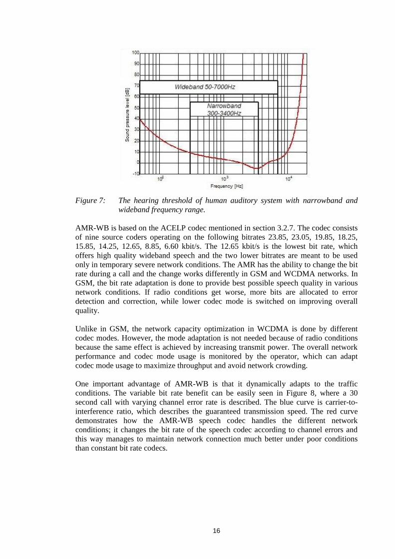
"f" and "s". The human hearing threshold curve is also very sensitive at frequencies
between 3400-7000 Hz.
16
Figure 7: The hearing threshold of human auditory system with narrowband and
wideband frequency range.
AMR-WB is based on the ACELP codec mentioned in section 3.2.7. The codec consists
of nine source coders operating on the following bitrates 23.85, 23.05, 19.85, 18.25,
15.85, 14.25, 12.65, 8.85, 6.60 kbit/s. The 12.65 kbit/s is the lowest bit rate, which
offers high quality wideband speech and the two lower bitrates are meant to be used
only in temporary severe network conditions. The AMR has the ability to change the bit
rate during a call and the change works differently in GSM and WCDMA networks. In
GSM, the bit rate adaptation is done to provide best possible speech quality in various
network conditions. If radio conditions get worse, more bits are allocated to error
detection and correction, while lower codec mode is switched on improving overall
quality.
Unlike in GSM, the network capacity optimization in WCDMA is done by different
codec modes. However, the mode adaptation is not needed because of radio conditions
because the same effect is achieved by increasing transmit power. The overall network
performance and codec mode usage is monitored by the operator, which can adapt
codec mode usage to maximize throughput and avoid network crowding.
One important advantage of AMR-WB is that it dynamically adapts to the traffic
conditions. The variable bit rate benefit can be easily seen in Figure 8, where a 30
second call with varying channel error rate is described. The blue curve is carrier-to-
interference ratio, which describes the guaranteed transmission speed. The red curve
demonstrates how the AMR-WB speech codec handles the different network
conditions; it changes the bit rate of the speech codec according to channel errors and
this way manages to maintain network connection much better under poor conditions
than constant bit rate codecs.

17
Figure 8: AMR-WB codec mode adaptation in GSM full rate channel
(Carrier-to-Interference ratio, C/I) [11].
The channel error repairing is managed by power control. This means that if the radio
conditions are weak, the transmission power is increased. The benefit from changing bit
rate is the increased network capacity to handle more customers in peak periods by
decreasing the speech coding bit rate.
The bit rate in AMR-WB can be selected asymmetric. It means that during a phone call
the uplink bit rate from a phone towards the base station can be different to the
downlink from the base station to phone. The speech frame length is 20 ms and the
operating mode can be changed often. When the network conditions change and the
suitable operating mode has to be selected, the phone uses the autonomous mode
forcing the bit rate to a different level.
4.3 Encoder
The AMR-WB speech codec is based on ACELP, which means that the AMR coding
method belongs to source coders. Source coders have lots of computation in their coder
and the six phased block diagram of AMR can be seen in Figure 9. Pre-processing is
done to all speech frames, as well as short-term LPC prediction and speech fundamental
frequency analysis. The codebook searches are performed in sub frames. The specific
information of the coder can be found from [14].

18
Figure 9: Simplified block diagram of the GSM Adaptive Multi-Rate encoder [14],
[32].
In pre-processing the high pass filtering and signal level decreasing are performed. The
reason for high pass filtering is that the unwanted low level signal components are
removed. The analysis of the LPC, LTP and fixed codebook parameters at a 12.8 kHz
sampling rate are performed. Thus a 16 kHz input signal has to be decimated.
The linear predictive analysis (LPC) is a way to approximate a speech sample as a linear
combination of past speech samples. By minimizing the sum of the squared differences
between the actual speech samples and the linearly predicted ones, a unique set of
predictor coefficients can be determined. The short-term prediction is performed using
an autocorrelation function with a 30 ms asymmetric window. To help computation, 5
ms in both directions from a window is used as an overhead.
The pitch-lag is related to the speech fundamental frequency analysis or long term
prediction analysis. Accurate estimation of the pitch-lag parameter is important for the
subjective quality of the synthesized speech. The search for pitch-lag parameter is
divided into two parts: The approximation for pitch-lag value is found with an open-
loop pitch search, which speeds up and limits the closed-loop pitch search done in an
adaptive codebook search. The closed loop refines the open-loop result by finding the
optimal value in the neighborhood of the open-loop result. The parameters for the
adaptive codebook are the delay and gain of the pitch filter. An open-loop pitch search
is done in every other sub frame in the adaptive multi-rate codec. Instead of frequency,
the time between the voiced sound pulses is measured.
Synthesis and weighting filters are updated for calculating the next sub frame stimulus
signal in a filter memory update. The adaptive and fixed codebook gains are vector
quantized using a 6 or 7 bit codebook.
19
Finally, the speech frame is complete and the result is an amount of parameters
quantized with a certain accuracy. The parameters are used in the receiver end in the
decoder and a signal similar to the original is reconstructed.
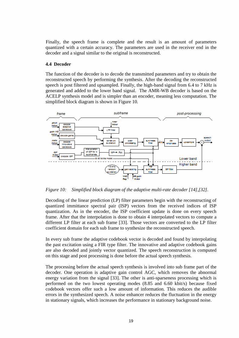
4.4 Decoder
The function of the decoder is to decode the transmitted parameters and try to obtain the
reconstructed speech by performing the synthesis. After the decoding the reconstructed
speech is post filtered and upsampled. Finally, the high-band signal from 6.4 to 7 kHz is
generated and added to the lower band signal. The AMR-WB decoder is based on the
ACELP synthesis model and is simpler than an encoder, meaning less computation. The
simplified block diagram is shown in Figure 10.
Figure 10: Simplified block diagram of the adaptive multi-rate decoder [14],[32].
Decoding of the linear prediction (LP) filter parameters begin with the reconstructing of
quantized immittance spectral pair (ISP) vectors from the received indices of ISP
quantization. As in the encoder, the ISP coefficient update is done on every speech
frame. After that the interpolation is done to obtain 4 interpolated vectors to compute a
different LP filter at each sub frame [33]. Those vectors are converted to the LP filter
coefficient domain for each sub frame to synthesize the reconstructed speech.
In every sub frame the adaptive codebook vector is decoded and found by interpolating
the past excitation using a FIR type filter. The innovative and adaptive codebook gains
are also decoded and jointly vector quantized. The speech reconstruction is computed
on this stage and post processing is done before the actual speech synthesis.
The processing before the actual speech synthesis is involved into sub frame part of the
decoder. One operation is adaptive gain control AGC, which removes the abnormal
energy variation from the signal [33]. The other is anti-sparseness processing which is
performed on the two lowest operating modes (8.85 and 6.60 kbit/s) because fixed
codebook vectors offer such a low amount of information. This reduces the audible
errors in the synthesized speech. A noise enhancer reduces the fluctuation in the energy
in stationary signals, which increases the performance in stationary background noise.

20
For high frequencies from 6.4 to 7 kHz, an excitation is generated first to model the
frequency range. The high frequency part is generated by filling the higher part of the
spectrum with white noise, which is scaled in the excitation domain. After this the
conversion to the speech domain is done by shaping the content with a filter derived
from the same linear predicting (LP) synthesis filter used for synthesizing the
downsampled signal. Before the speech signal is obtained the high-band speech is
filtered with a LP and band pass filter from 6.4 to 7 kHz. Finally, the synthesized higher
band signal is added to the lower band synthesized speech and the final output speech
signal is completed.

21
5. MOBILE PHONE ACOUSTICS
In this chapter several factors that affect the quality of heard sound from mobile phone
earpieces are presented. First, the processing of incoming audio from the speech
decoder to the loudspeaker is introduced. After that the mechanical part is described by
introducing the dynamic loudspeaker, and enclosures with leak types and reasons for
certain mechanical selections are discussed.
5.1 Audio path from mobile phone’s antenna to speaker
When a mobile phone antenna receives the speech signal from the sender, lots of signal
processing is done before the audible sound from the loudspeaker. A rough description
about the downlink path blocks from the speech decoder to the earpiece is shown in
Figure 11. The important block is speech enhancements, which includes for example
noise cancelling for removing the noise from received speech and multiband dynamic
range controller (MDRC), which is described later in Figure 12.
The equalizer is needed correcting the magnitude response of the earpiece. If the
loudspeaker cannot produce enough for instance low frequencies, the equalizer
parameters can be tuned to increase the signal level on low frequencies. However, one
disadvantage of this operation is increased distortion. The problem with an equalizer is
that it fails to take the input signal level into account. This means that if the input signal
is already loud before the equalizer, in the worse case, it is gained over the theoretical
limits, which inevitable leads to noticeable distortion in the earpiece.
Upsampling from 16 kHz to 48 kHz is done to support a suitable sampling rate to the
hardware audio codec. In the last block in the digital domain, the signal is converted
from the digital to analog domain in the digital-to-analog (D/A) conversion block.
In the analog domain, the lowpass filter removes unwanted signal components before
amplifications. Finally, the analog gain has to be adjusted to a suitable level for the
earpiece. Before the earpiece a few passive components are added to protect the
earpiece for instance from voltage peaks.
Figure 11: Simplified block diagram of the mobile phone earpiece downlink.

22
An important part of downlink audio path is the dynamic range controller DRC. A
common feature of the DRC is that the input signal level is detected continuously, and
according to this detection, a defined amplification to signal is performed [34]. The
mentioned MDRC is an extension for the DRC, a device that divides the full frequency
band into sub-bands, which are amplified separately. There are different ways to realize
the DRC [34], but this thesis concentrates on the functional part of it. The basic
principle is shown in Figure 12 and the meaning of different parts are explained below:
- Signal deleted: If the input signal level is very low the output signal is deleted by
dropping the signal level for example -100 dBFS. Usually this kind of weak input
signal level is noise and deleting it is natural to enhance SNR.
- Expansion: The level of quiet input sounds are increased and the dynamic range of
the audio output signal is also increased. The steepness of this part is critical, because
if the expansion is done too steep the low speech signal levels can be partly lowered
resulting in audible errors in the earpiece. If the expansion is too mild, unwanted
noise may be added to the output signal.
- Amplification: In this stage the input speech signal is amplified for instance 15 dB.
The input speech signal is somehow normalized in the uplink and the amplification
area is adjusted to be long enough to cover most of the speech signal.
- Compression: In simple terms, the loud sounds over a certain threshold are reduced,
in this case the input signal limit is -30 dBFS. The operation decreases the dynamic
range of the speech signal, but the advantage is that loud signal levels in a noisy
environment are not amplified too much.
- Limitation: To prevent the loud output signal to reach the loudspeaker, the loudest
output signal level is limited according to the loudspeaker performance. If the
limitation is neglected, a considerable amount of distortion may be added to the
output signal.
Figure 12: Dynamic audio compressor/expander level response [34].

23
The DRC was introduced in this section because even its performance is not shown in
the frequency response and distortion measurements, it affects the end-user experience
heard from the earpiece especially in expansion and limitation parts.
5.2 Audio module in mobile phones
The speaker plays an important role but acoustics matter as well. Phones with similar a
earpiece can differ from each other due to different acoustics. The dynamic loudspeaker
is introduced with different enclosures to give an idea of possible factors that affect the
sound quality.
5.2.1 Dynamic loudspeaker
The dynamic loudspeaker is the most common speaker type in the loudspeaker industry.
In practice, all speakers used so far in mobile phones are dynamic loudspeakers.
The basic idea of dynamic loudspeakers is to convert the electrical signal to an
acoustical signal [18] and can be described as a four-pole model as in Figure 13. The
input side has voltage and current, where as the output volume velocity and sound
pressure. With the alternating current in a magnetic field the force tries to move the
compact coil of wire. If the coil is attached to a large surface it moves the air more
efficiently giving volume velocity to the air, which is heard as a sound.
Figure 13: Four-pole network of the speaker [18]. Symbols are: e = input
voltage, i = current, Zg = impedance of electrical circuit, q = volume
speed of oscillator, p = sound pressure, Zrad = radiation impedance [18].
The current in a wire in a magnetic field produces a force on the wire. If a single wire is
moving in a uniform magnetic field it represents the simplest coil transducer. The coil
experiences force in the axial direction and the total force is:
𝐹𝑚𝑎𝑔 = 𝐵𝑙𝑖, (26)
where 𝐹𝑚𝑎𝑔 is the force produced by a current i [N], 𝐵 is a magnetic-flux density in tesla
[T], 𝑖 is the alternating current in amperes [A] and 𝑙 describes the length of wire in the
magnetic field [m].
The moving coil loudspeaker system can be presented with an acoustical equivalent
circuit described by Hall [28]. By taking a closer look at Figure 14, the speaker is
described by an electro-mechano-acoustical circuit. The coil has electrical resistance Re
and inductance Le. The amplifier with output impedance Zg supplies voltage Eg which
drives current ig through the coil. This causes force F=Bli on the cone and coil, with
resulting motion v. The cone and coil are considered as a mechanical system with a
mass m and mounting stiffness Cm , including flexing of the material resistance Rm.
After that, the volume velocity U=vA, where v is the mechanical velocity of the

24
membrane and A is cone area A. Volume velocity U works against the radiation
impedance Za,rad of the surrounding air to generate sound pressure p.
Figure 14: Electro-mechano-acoustical circuit of moving coil loudspeaker system.
The symbols are explained above the figure in the text [28].
The structure of a dynamic loudspeaker is quite simple. Usually the wire is wrapped as
a coil and situated between the magnetic poles. The purpose is to maximize the length
of the wire where the magnetic field is constant and perpendicular to the wire. As
mentioned earlier neither the coil itself does move much air, nor produce sound. The
efficiency is increased by attaching the coil to a movable, light and relatively large
surface diaphragm which carries lots of air along with it. Low frequencies generally
need a larger radiating area, whereas high frequencies are produced with a smaller area.
In larger speakers, or home stereo speakers, the diaphragm is usually a cone, which is
fairly stiff and light. The diaphragms in small speakers used in a mobile phones are also
quite stiff even though the material is thin.
By looking at Figure 15 the main parts [27] of the dynamic loudspeaker are shown in a
cross-section picture. However, exactly this kind of shape is not used in mobile phone
earpiece, but the principle is the same.
Figure 15: Cross-section sketch of a dynamic loudspeaker [27].
To minimize the non-linear response, the permanent magnet must be selected to
produce a constant field and the voice coil should always have the same amount of turns
in every displacement inside the gap between the poles [29]. The movement area of the

25
voice coil has to be limited in the constant field area, because if a coil exceeds that area
the magnetic force Bl drops causing non-linearity. Another problem occurs if the
speaker diaphragm movement distance is too long and exceeds the linear operation area,
which may cause mechanical damage to the speaker. In order to reduce impedance
variation, the chassis is made either to be able to conduct the heat away from the voice
coil or the chassis endures high temperatures and this way the voice coil stays in a
stable condition even in harder usage.
Voice coil suspensions keep the speaker membrane accurately centered in the magnet
gap, which is important enabling only the axial direction movement. One other function
of the suspension is that, when there is no signal, the membrane is returned back to the
equilibrium position.
The main reasons for using a dynamic speaker are the low operational voltage, small
size and low price. There are some drawbacks like low efficiency (usually 1%) and
frequency response, which is poor at low frequencies due small effective radiating area
and short membrane movement distance. The simulation of enclosure and speaker
element for design purpose is fairly straightforward due to the long history of dynamic
transducer studies.
5.2.2 Leak types, front and back cavity
A loudspeaker without an enclosure design does not provide very good acoustic
performance. Usually there are lots of compromises in mobile phone acoustic design
due purpose of use or mechanical design. The main purpose of mobile phone earpiece is
to reproduce speech, which has been narrowband until these days. In upcoming years,
there will be a need for wideband capability and that must be taken into account when
designing the acoustics for mobile phones. Therefore the front and back cavities with
different leak types are introduced in this section.
The front of the loudspeaker
There are two main possibilities to realize the front part of the speaker, called the front
resonator and open front.
Front resonator: The front cavity usually consists of the cavity itself and a cover with
sound holes. The purpose of the front cavity is to boost high frequencies thus reduce the
need for equalization. The other function is to provide protection against dust, water and
other external damage, which could be harmful for the speaker without the front cavity.
The disadvantage of the front cavity together with the sound holes is that it is a new
source of tolerance errors, but proper front cavity design can decrease the amount of
tolerance effects. Also, the cavity requires space, which is not available adequately in
mobile phone.
Open front: If there is no space for a front cavity, the speaker can be placed so near the
phone cover that the cavity is very small or does not exist. This way the acoustic
resonances are shifted to higher frequencies above the speech band, but the boosting
effect of the front resonator for the higher speech frequencies in the usable band is lost.
This leads to much heavier DSP equalization. In addition, the open-front design does
not include a lowpass feature, which can be used to filter out unwanted for example
radio frequency (RF) buzzing noise just above the speech signal band. Both of the
explained implements are shown in Figure 16.

26
Figure 16: Different mobile phone earpiece front realizations [31].
Back side of the loudspeaker
There are four main design and various hybrids available for designers to choose for the
back side of the loudspeaker.
Open back: The back of the loudspeaker is left open to the space of air inside the phone.
This method is the most common in all earpieces [31]. Even if the sound from the back
of the loudspeaker is routed through the PWB behind the speaker, the realization is
called open back. The advantages are ease of design and small space consumption.
Problems can occur on low frequencies if a large external leak is included in the
mechanics.
Closed back: In this case the loudspeaker has its back enclosed in a cavity that is sealed
or contains a small acoustically damped leak. The leak is only connected to ambient air
or air inside the phone, not to the ear. The good side of this is the isolation to the
microphone though the air path inside the phone. The downside is that the cavity should
be large, around a few cm3. In practice, the open back realization is preferred for its
small space occupation offering almost as good a result as the closed back.
Vented: The idea in vented back enclosure is to work as a bass booster. The earpiece has
a back cavity that is hermetically sealed apart from an opening with a defined cross-
sectional area and length (pipe) behind the loudspeaker. The gained resonator is tuned
near the lower limit of the frequency range of the earpiece. To make the vented structure
to work, the outer end of the vent has to be routed directly or indirectly to the user's ear.
If this is neglected and the vent is left inside the phone without acoustical connection to
ear, the performance will be worse than with other implementations. The reason for
using this design is the boosting effect for low frequencies with lower distortion thus it
is well suited for a small speaker in wideband designs. The problem with this design is
the same as with closed back design, which is the required large cavity.
Tube-loaded: The realization is about the same as vented construction, but this case the
cavity is much smaller and the vent is narrower and longer. The advantage of this
method is small bass boost, which is important in wideband implementations. Even a
relative small speaker with stiff suspension can reach low frequencies but the speaker
has to handle the required higher displacement.

27
Figure 17: Four different earpiece enclosure back types used in mobile phone [31].
Leak types
Basically there are three different types of leak to put into practice shown in Figure 18.
No leak: When the phone is held against the ear, only the natural leak between the ear
and the surface of the phone cover is present. This kind of leak is the simplest of all
realizations having high leak tolerance, which means that the sound of the earpiece is
relatively insensitive to variations in the leak between the phone and the ear.
External leak: This case an intentional acoustic leak lets some of the sound pressure
escape from the ear to the ambient air outside. The leaking occurs even if the phone is
sealed against the ear. This type of design is common and works well increasing further
leak tolerance. Also the tuning is easier due the leak.
Internal leak: The idea is the same as the external leak, except the leak is going from the
front cavity to the ambient air. Usually this realization performs worse than the external
leak implementation due to equalization for high frequencies. The internal leak option is
not recommended, except if the earpiece and integrated hands-free (IHF) speaker have
to be combined or lack of space prevents other leaks in the phone cover.
Figure 18: Different leak types used in mobile phone earpiece enclosure [31].
5.2.3 Loudspeaker implementation in different phone models
As presented earlier in Chapter 5, good performance depends on many things. There are
many rival parameters affecting the size of the loudspeaker and enclosure selections.
The planned phone price defines quite much for example the components that there will
be in the phone. Mechanical design limits or allows modifications to acoustics as well.
Some of these factors are listed below:
Narrowband or wideband phone
Phone price

28
Dust and water protection
Mechanical design
Designer's set of parameters
If the phone is a wideband model the requirement for earpiece sound production
performance is different to narrowband. Using the small speaker gives more space for
other components in the phone and can be cheaper, but the low frequencies on
wideband cannot be reproduced as purely, or at all, as with a larger speaker. The
mechanical design containing cavities and leaks described earlier with DSP may help,
but a speaker has its limits and cannot break the physical laws. If the speaker is large,
lousy mechanical design or audio designers tuning parameters may be ruining the
advantages that could have been achieved by the speaker. On the other hand, using a
large speaker gives more margin to audio designers compared to small speakers.

29
6. OBJECTIVE MEASUREMENTS
It is important to show the objective results, when the subjective results are analyzed.
The purpose of objective measurements is to find out if there is any distinct differences
between the speakers 1) without the phones, 2) integrated to the phones without audio
processing and 3) integrated to the phones with audio processing. First, the theory of
objective measurements is presented and then the measurements with results of the used
phones and speakers are shown in this chapter.
6.1 Theory of audio measurements
Before the measurement results the theory behind the objective measurements are
presented in the next three sections. Impulse response, frequency response and
distortion methods are described to help to understand the measurement results later in
this chapter.
6.1.1 Transfer function
The transfer function describes an ideal system behavior with any kind of stimulus. An
ideal physical system has four properties [21]:
1) The system can be physically realized means that the system cannot produce an
output before input is applied.
2) Constant of its parameters when the system is time invariant thus the response of the
system is constant for all time values.
3) Stability limits the system's output to be a finite signal for a finite input signal.
4) A Linear system is additive and homogeneous. If the output signals are 𝑦1and 𝑦2 with
input signals 𝑥1 and 𝑥2. An additive system produces a summed output 𝑦1 + 𝑦2 from
summed input 𝑥1+ 𝑥2. A homogeneous output 𝑐𝑦1is produced from input 𝑐𝑥1, where c is
a random constant.
Figure 19: Linear, ideal system h(t) with one input x(t) and output y(t) signals [21].
The unit impulse function is defined as follows:
h(t) = y(t)
when
x(t) = (t)
Where h(t) is unit response function of the system, y(t) describes the output of the
system, x(t) input of the system and (t) is the ideal impulse, i.e. delta function, t is the
time from the moment when delta function enters the system. The duration of ideal
impulse is defined to approach to zero, so, in other words, the duration is infinitely
short. Also, the amplitude and energy is defined to be infinity and the integral equals 1
[22]. If the ideal impulse would be used for measuring the speakers of phones in this

30
thesis, the results with good signal-to-noise ratio would contain a high amount of
distortion, or even worse, break the speakers. It is obvious that these kind of parameters
are not for the practical part of this thesis but only for theory.
Instead of using the theoretical and unpractical method mentioned earlier, sine sweep is
used to measure the frequency response of the speakers. The simplest form of sine
swept frequency measurement is linearly or logarithmically variable sine wave, which is
fed to the device under measurement, DUT. Output signal represents the magnitude
response of the device.
Because the sinusoidal stimulus contains energy concentrated instantaneously at one
frequency, noise and other artifacts disturbing the measurement can be filtered away by
using tracking filter, i.e. a narrowband bandpass filter. One advantage of sine sweep is
its ability to measure simultaneously frequency response and the non-linear distortion
[36]. According to Farina in [36], from a sine signal used in an exponentially varied
frequency, it is possible to deconvolve simultaneously the linear impulse response of the
system and separate impulse responses for each harmonic distortion order.
6.1.2 Frequency response
When the system's output spectrum in response to an input signal is of interest, the
frequency response is the right measure. It often helps designers to implement systems
by offering additional information about the system behavior. The characteristics of the
system can be illustrated by a linear transform of the unit impulse response. The
transform function of a system can be represented in the Laplace form of the impulse
response.
𝐻 𝑠 = (𝑡)𝑒−𝑠𝑡𝑑𝑡∞
0 (27)
where H(s) is the complex-valued transfer function of a system and 𝑠 = 𝜎 + 𝑗𝜔
describes the complex frequency variable. The Laplace function, like the impulse
response is defined to begin at t = 0.
The most powerful method to represent the response in the frequency domain is the
Fourier transform [21] of the impulse response.
𝐻 𝑓 = 𝑡 𝑒−𝑗2𝜋𝑓𝑡∞
0𝑑𝑡 (28)
where H(f) is the complex frequency response of the system and f is the real-valued
frequency. When 𝜎 = 0 the Fourier transform (28) becomes the transfer function (27)
and it is investigated on the 𝑗𝜔-axis. The transfer function is not very practical and,
therefore, the frequency function is used instead. Usually, the absolute value of the
frequency response called the magnitude response |𝐻 𝑓 | describes the frequency
response curves.
The transform domain representation can be inversed to the time domain by inverse
Laplace in the s-domain or Fourier in the f-domain transform.
𝑡 =1
𝑗2𝜋 𝐻 𝑠 𝑒𝑠𝑡𝑑𝑠
𝜎+∞
𝜎−∞ (29)
𝑡 = 𝐻(𝑓)∞
−∞𝑒𝑗2𝜋𝑓𝑡𝑑𝑓 (30)

31
where 𝜎 is the real part of the complex frequency variable s.
6.1.3 Distortion
If a speaker with a completely linear transfer function would produce an identical output
signal compared to input signal there could not be any distortion. It is not a surprise that
a small speaker in mobile phone, capable of producing high sound pressure level cannot
play undistorted sound. The nonlinear distortion produces unwanted signal components,
which does not exist in original signal and adds them to the output signal.
The harmonic distortion appears on a clean sine sound in harmonic components. If the
spectrum of the signal consists of fundamental frequency A(1) and the amplitude of 𝑖𝑡 harmonic component A(i), the total harmonic distortion (THD) is defined [1] as
𝑑 = 100% 𝐴(𝑖)2𝑁
𝑖=2
𝐴(𝑖)2𝑁𝑖=1
(31)
where d is harmonic distortion, 𝐴(𝑖) is amplitude of 𝑖𝑡 harmonic component and N is
the number of harmonic components.
The distortion measurements in this thesis are done with all non-harmonic components,
background noise and noise from measurement equipment. This kind of distortion is
called THD+N. Not all distortion is a bad thing, mentioned in [1] that low order
harmonics can make the speech sound more pleasant in a telephone line than
undistorted speech.
6.2 Earpiece measurements in free field
The phones under measurements and the listening test have different size of speakers.
The physical measurements of the speakers are shown in Appendix A: and Appendix
B:. Those two speakers were measured in free field to obtain information about the
speaker performance before integrating it to the mobile phone. Both of the earpieces
were measured by Lauri Veko in the anechoic room (AR1) at the Salo Nokia premises
in November 2007.
6.2.1 Earpiece measurement procedure and equipment
The earpieces that were under evaluation were measured in the International
Electrotechnical Commission (IEC) standard baffle (a plate with a hole for speaker).
The used measurement setup was the following: The measurement adapters for both
speakers were free air adapters and designed for those two speakers. Basically, the
adapter had a hole in the front part, where the component sound hole was and the back
part was open. The measuring distance between the speaker and 1/4" free field
microphone was 1 cm. The whole measurement setup is shown in Figure 20. The
measuring equipment is listed in Table 2.
Table 2: Test equipment used in measurements of the earpieces in a baffle.
Instrument Type Comment
Audio Audio Precision Control software
measurement System Two ApWin
system Cascade

32
Instrument Type Comment
Audio Audio Precision Amos XG controls
Precision 2700 series Audio Precision, ApWin
Condensator B&K Type 4939 1/4" mic + its preamp
microphone + B&K Type 2670
preamplifier
microphone B&K Nexus Mic amplifier
amplifier
Impedance box 1ohm Shunt resistor
Rotel amplifier Speaker
amplifier with fixed gain +6dB amplifier
Figure 20: Speaker measurement set-up. A PC controls the Audio analyzer, which
brings the measurement data back to the computer.
6.2.2 Results of earpiece measurements
The speakers under evaluation were measured in a frequency range from 200 Hz to 20
kHz. The results of the frequency response measurement can be seen in Figure 21 and
distortion in Figure 22. The input voltage for both measurement was set to 0.179 Vrms.
Frequency response of the earpieces
If the wideband codec frequency range 50 - 7000 Hz is examined from the Figure 21,
the high frequency area near 7 kHz is about the same for both speakers. On the other
hand, at low frequencies, the small speaker performance is clearly worse than for the
large one. In fact, the frequencies under 400 Hz are 10 dB more silent on the small
speaker, which is not possible to compensate in the mechanical design and, therefore, is
seen later in earpiece integrated to phone in Section 6.3 results.
As can be seen from Figure 21 the large speaker frequency response curve -3 dB point
is around 300 Hz, when the small speaker has it at about 500 Hz. Also, the frequencies
between the two resonance peaks (big speaker 400 Hz-5000 Hz, small 600 Hz-7000 Hz)
varies in the large speaker only 4 dB and the small one 7 dB.

33
Figure 21: Small and large speaker frequency response in frequency range 200 Hz -
20 kHz measured with free air adapter.
Distortion in earpieces in free field
Distortion on both speaker is plotted in the same Figure 22 and notable thing is that
background noise is also included in the results. However, the small speaker has more
distortion below 650 Hz ending up to 11%. The frequency band is from 200 Hz to 20
kHz.
50
60
70
80
90
100
100 1000 10000
Mag
nit
ud
e r
esp
on
se [
dB
SP
L]
Frequency [Hz]
Speaker Frequency Response at 1mW (0.179Vrms)
Small speaker Large speaker

34
Figure 22: Small and large earpiece total harmonic distortion and noise in frequency
range 200 Hz - 20 kHz measured with free air adapter.
6.3 Measurement for wired earpieces integrated to Nokia mobile phone
After the free field measurements in Section 6.2, the speakers' performances can be
compared more or less in a theoretical aspect. If a speaker is measured in a free field
adapter it does not sound the same way when placed in a proper enclosure. Measuring
the earpieces wired to the phone means that the earpieces are integrated to the real
phone without the audio signal processing. Using the HATS' ear for measurement, the
results are one step closer to the end-user experience.
6.3.1 Selection criteria's for phones in the test
The phones that are measured in the next sections are introduced shortly before the
measurement procedure. Both of the phones were selected for this thesis on three
criterias: 1) Phones have different sized speakers 2) Support for AMR-WB codec
available, 3) is available on the market thus is not just a prototype. The other phone is a
Nokia 6220 classic introduced in Q208. It has the small speaker measured in Section
6.2. The other is the wideband phone, the Nokia 6720 classic, introduced in Q209.
Furthermore, it contains the large speaker.
6.3.2 Measurement equipment and procedure for wired earpieces
The idea of this measurement is to get data about the speakers integrated to the phone
without the influence of audio signal processing. The phones were positioned to HATS
according to the designers directions (Appendix F: and Appendix G:) and the phone
earpieces were wired directly to Audio Precision through a B&K power amplifier. After
the HATS ear the microphone signal was amplified in the B&K microphone multiplexer
and connected to a PC through Audio Precision. A block diagram of the measurement is
shown in Figure 23.
0,1
1
10
100 1000 10000
TH
D+
N [
%]
Frequency [Hz]
Speaker Total Harmonic Distortion and Noise at 1mW (0.179Vrms)
Small speaker Large speaker

35
Table 3: Used measurement equipment in HATS measurement by wiring the
earpieces directly to the power amplifier.
Instrument Type Comment
Audio Audio Precision Control software
measurement switcher Type ApWin
system SWR 2122
Audio Audio Precision Amos XG controls
Precision 2700 series Audio Precision, ApWin
Power B&K Type WR1105 Loudspeaker
amplifier amplifier
Microphone B&K Type 2822 Microphone
multiplexer amplifier
Before the actual measurement, the phone covers were opened and wires were soldered
to the earpiece springs. The proper soldering was confirmed with a multimeter by
measuring the speakers' resistances, which were about 30 Ω.
Figure 23: Measurement setup for phones measured on HATS by wiring the
earpieces.
The voltages used in the measurement were defined by Audio Precision and are
presented in Table 4.
Table 4: The input voltages for phone earpieces measured on HATS.
Type Input level [dBV] Input level [mVrms]
ERP -20 114
DRP -20 114
DRP -15 202.7
DRP -10 360.5
DRP -5 641.1

36
6.3.3 Results of the wired earpiece measurements on HATS
After the measurements Audio Precision plotted the results to Excel. The frequency
response and distortion results are shown below.
Frequency response
When phone measurements on HATS are plotted for different voltages, it can be seen
that the speaker performance is noticeably different, especially at lower frequencies.
There is a possibility to measure frequency response with ear-drum reference point
(DRP) or without ear reference point (ERP) the influence of HATS' ear auditory canal.
The reason for using DRP is that ERP measurement does not contain distortion
measurement in Audio Precision due to unlinear distortion at different frequencies.
Filtering the unlinear distortion would not be such a successful process. However, the
behavior of the speaker integrated to the phone is clearly shown in the DRP
measurements.
Figure 24: Frequency responses on range 100 - 8000 Hz measured on HATS using
different input voltage levels in N6720c and N6220c speakers.
The Ear Reference Point (ERP) results are shown for comparison for full audio path
measurements in Section 6.4. The Nokia 6220c is sealed on the HATS ear better than
the Nokia 6720c, which can be seen in Figure 25 at frequencies lower than 1 kHz. The
boosting effect from sealing helps the designer's tuning work to get the phone to fit into
the 3GPP frequency response mask. The descent of the frequency response of the Nokia
6220c from 600 Hz to 100 Hz is steeper than for the Nokia 6720c.
-20
-10
0
10
20
30
100 1000 10000
dB
Pa
Frequency [Hz]
Earpiece Power Compression on HATS DRP
Nokia 6220c -20dBV Nokia 6220c -15dBV Nokia 6220c -10dBV Nokia 6220c -5dBV
Nokia 6720c -20dBV Nokia 6720c -15dBV Nokia 6720c -10dBV Nokia 6720c -5dBV

37
Figure 25: Phones measured on HATS ERP position on frequency range 100 - 8000
Hz. HATS' ear effect is filtered away by Audio Precision measurement
system. THD+N
In the earpiece total harmonic distortion and noise (THD+N) measurement on different
voltages, the small speaker performs considerably poorly compared to the large speaker.
The distortion begins to rise faster than the large speaker under frequencies of 700 Hz.
The frequencies under 450 Hz for the small speaker THD+N results are inaccurate due
the incapability of reproducing such low frequencies. Basically, the membrane is so
small that sound production is impossible at those frequencies.
-20
-10
0
10
20
30
100 1000 10000
dB
Pa
Hz
Earpiece Frequency Response at -20 dBV at ERP
Nokia 6220c Nokia 6720c

38
Figure 26: Nokia 6720c and 6220c THD+N on different earpiece input voltages on
HATS. Measured frequency range is 100 - 8000 Hz.
6.4 Nokia mobile phone measurements over the air
The objective 3GGP [26] measurements of two Nokia phone models are shown in this
section. The idea is to compare over the air results to the speaker measurements done in
Section 6.2. It is also important to get information about the speaker integration and
audio path effects in the measurement results. These results describe the end user
hearing experience during a call.
6.4.1 Information about the phones in the test
All mobile phones that are on the market have been measured in a type approval test.
For this test, the designer defines the nominal volume level, which is a volume level
between 2/10-9/10. The selected nominal volume levels for both phones are shown in
Table 5. These volumes were used because the phones have been tuned to fit to the
masks on these specific levels.
Table 5: Nominal volumes of two Nokia phones.
Nokia 6220c
narrowband
Nokia 6220c
wideband
Nokia 6720c
narrowband
Nokia 6720c
wideband
Nominal volume 5 4 6 6
The AMR-WB speech codec was enabled in both phones for the tests.
0
10
20
30
40
50
100 1000 10000
Dis
tort
ion
%
Frequency [Hz]
Earpiece THD+N on HATS
Nokia 6220c -20dBV Nokia 6220c -15dBV Nokia 6220c -10dBV Nokia 6220c -5dBV
Nokia 6720c -20dBV Nokia 6720c -15dBV Nokia 6720c -10dBV Nokia 6720c -5dBV

39
6.4.2 Measurement equipment and procedure
Both of the phones were measured on HATS with 3GPP specification release 7 [26].
3GPP specifies test methods to allow the minimum performance requirements for the
acoustic characteristics of GSM and 3G terminals for both narrow and wideband. The
used measurement equipment in 3GPP measurements were proceeded with the list of
instruments in Table 6. This is the only measurement where Audio Precision was
replaced by Audio analyzer UPL-16.
Table 6: Equipment used in 3GPP measurements.
Instrument Type Comment
Radio Rohde & Schwarz GSM & WCDMA
communication CMU 200 network used
tester
Rohde & Schwarz Audio analyzer Sents result data to PC
UPL-16 Amos XG controls it
Head And Torso B&K Includes artificial ear
Simulator with microphone
microphone B&K Nexus HATS mic amplifier
amplifier +20dB
Once the phone was positioned to HATS the measurement was started. A PC controlled
the UPL, which fed the measurement signal to the radio communication tester and the
phone earpiece speaker signal was measured on the HATS' ear. Finally, the recorded
signal from the HATS ear is amplified 20 dB with B&K Nexus. The procedure is shown
in Figure 27.
Figure 27: Measurement setup for phone speaker frequency response and
distortion.
A picture of HATS used in this measurement and later in Section 7.2 for recording the
files for subjective test is shown in Figure 28.

40
Figure 28: Nokia 6720 classic positioned to 3GPP measurements HATS in
anechoic chamber.
Network settings for both phones were as in Table 7.
Table 7: CMU network settings in 3GPP HATS measurement.
GSM WCDMA
PCL 5 Uplink 1852.4 MHz
TCH 35 Downlink 1932.4 MHz
Codec mode 12.20 kbits Codec mode 12.65 kbps
Speech codec low Speech codec low
6.4.3 Measurement results
To ensure that the phone to be used in the recordings for subjective test is not a faulty
one, five phones of each model were measured. An average phone was selected based
on frequency response and distortion measurements. Differences in results between the
measured phones results were mostly inside ±1 dB.
Frequency response
The frequency response follows the results in the previous Section 6.3.3. The Nokia
6720c has a flat response, while the Nokia 6220c fails to stay within the limits on
narrowband (red dash line in Figure 29).

41
Figure 29: Results from narrow and wideband earpiece frequency response
measurements of two Nokia phones on nominal volumes. Lower and
upper limits are solid line for narrowband, wideband lower limit is
marked with the dash line. The limits are from 3GPP version release 7.
Narrowband bit rate was 12.20 kbit/s whereas on wideband it was 12.65
kbit/s.
Distortion
Distortion is presented as separate figures for narrowband and wideband to clarify the
plotting. The Nokia 6220c performs worse on both narrow and wideband at volume
levels 4/10 and 5/10.
-30
-20
-10
0
100 1000 10000
Mag
nit
ud
e [
dB
r]
Frequency [Hz]
Receiving Frequency Response on HATS, Narrowband & Wideband
Upper limit
Lower limit narrowband
Lower limit wideband
Nokia 6220c Narrowband
Nokia 6720c Narrowband
Nokia 6220c Wideband
Nokia 6720c Wideband

42
Figure 30: Measured earpiece distortions on narrowband on nominal and maximum
volumes. Narrowband bit rate was 12.20 kbit/s and wideband bit rate was
12.65 kbit/s.
The difference between narrowband and wideband measurement result on the Nokia
6220c is emphasized by the volume level. The lower the volume, the more distortion
there is in lower signal levels.
Figure 31: Measured earpiece distortions on wideband using nominal and maximum
volumes. Narrowband bit rate was 12.20 kbit/s and wideband bit rate was
12.65 kbit/s.
0
10
20
30
40
50
60
-50 -40 -30 -20 -10 0
Ou
tpu
t SN
R [
dB
]
Input signal level [dB]
Narrowband Earpiece Distortion and noise on HATS, Nominal & Maximum Volume
Lower limit
Nokia 6220c Narrowband Volume 5
Nokia 6220c Narrowband Volume 10
Nokia 6720c Narrowband Volume 6
Nokia 6720c Narrowband Volume 10
0
10
20
30
40
50
60
-50 -40 -30 -20 -10 0
Ou
tpu
t SN
R [
dB
]
Input signal level [dB]
Wideband Earpiece Distortion and noise on HATS, Nominal & Maximum Volume
Lower limit
Nokia 6220c Wideband Volume 4
Nokia 6220c Wideband Volume 10
Nokia 6720c Wideband Volume 6
Nokia 6720c Wideband Volume 10

43
6.5 Discussions about the objective measurements
The objective measurements revealed expected differences between the small and large
speaker in capabilities of producing sound. The main reason for the differences in
results is the size of the earpiece membrane, which is discussed in the loudspeaker
theory Section 5.2.1 and seen in the free field measurement without being integrated to
the phone results in Section 6.2. After these it could be expected that there will be
differences in the results when the speakers are integrated to the phone and measured on
HATS.
Measurements on HATS illustrate the meaning of acoustics. If the measurements
without the phone audio processing are compared to 3GPP measurements where the
phone equalization and other audio enhancements are online, the results revealed that
audio processing can help to fix the problem by making the frequency response flatter.
The reason the frequency response is aimed to be flat is simply to avoid emphasizing or
diminishing certain frequencies, which could harm the understanding of hearing the
speech.
The incapability of reproducing low frequencies at a satisfying level for wideband
speech on a small earpiece can be seen from all measurements done in this chapter. The
distortion levels at different input voltage levels in Figure 26 revealed the unlinearity of
distortion on the small earpiece under frequencies of 450 Hz when the large earpiece
has fairly predictable levels until 100 Hz. In practice, the small earpiece may produce
audible distortion at low frequencies when the user sets the phone volume level to
maximum. Naturally, this limits the maximum output level that a designer can allow to
come out from the small earpiece without distortion. The other option is to damp the
low frequencies and allow the higher frequencies to sound louder. This option is
recommended only for narrowband speech and in the Nokia 6220c, the narrowband
speech is tuned to produce more higher frequencies (500 - 3000 Hz).
The differences of the two phone earpiece integration is shown on a theoretical level
and through objective measurements. The larger earpiece integration is 10 dB louder at
100 Hz and the fundamental frequency of male speech is around 100 Hz. After these
facts it can be said that the end-user should hear audible differences between the
realizations. The next chapter tries to find the answer to this and it is interesting to see
the subjective test results.
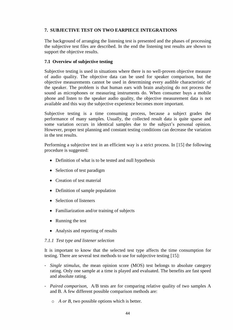
44
7. SUBJECTIVE TEST ON TWO EARPIECE INTEGRATIONS
The background of arranging the listening test is presented and the phases of processing
the subjective test files are described. In the end the listening test results are shown to
support the objective results.
7.1 Overview of subjective testing
Subjective testing is used in situations where there is no well-proven objective measure
of audio quality. The objective data can be used for speaker comparison, but the
objective measurements cannot be used in determining every audible characteristic of
the speaker. The problem is that human ears with brain analyzing do not process the
sound as microphones or measuring instruments do. When consumer buys a mobile
phone and listen to the speaker audio quality, the objective measurement data is not
available and this way the subjective experience becomes more important.
Subjective testing is a time consuming process, because a subject grades the
performance of many samples. Usually, the collected result data is quite sparse and
some variation occurs in identical samples due to the subject’s personal opinion.
However, proper test planning and constant testing conditions can decrease the variation
in the test results.
Performing a subjective test in an efficient way is a strict process. In [15] the following
procedure is suggested:
Definition of what is to be tested and null hypothesis
Selection of test paradigm
Creation of test material
Definition of sample population
Selection of listeners
Familiarization and/or training of subjects
Running the test
Analysis and reporting of results
7.1.1 Test type and listener selection
It is important to know that the selected test type affects the time consumption for
testing. There are several test methods to use for subjective testing [15]:
- Single stimulus, the mean opinion score (MOS) test belongs to absolute category
rating. Only one sample at a time is played and evaluated. The benefits are fast speed
and absolute rating.
- Paired comparison, A/B tests are for comparing relative quality of two samples A
and B. A few different possible comparison methods are:
o A or B, two possible options which is better.

45
o A or B scale, both samples are rated with the same scale.
o A or B scale with fixed reference is a test where one of the test samples is the
known reference and the other is a degraded from the reference.
o A or B scale with hidden reference is same as the previous but the reference is
not known, which enables either samples to be better.
- A, B or X test is made up of three samples. The idea is to choose, which one of two
samples, A or B is closer to the quality of X.
- A, B or C test is a triple stimulus comparison with a hidden reference. Two of three
samples are similar and one is the reference. The listener decides, which sample of
the other two samples is different to the reference and evaluates the sample.
- Rank order has several stimuli to compare. The relative order of the stimuli is rated.
Rapid ranking is a method of quality. The downside of it is that the perceptual
distance is unknown between the stimuli.
When the samples for the listening test were processed, it was time to decide the
listening test type. Because the differences between the small and large speaker are
rather small, the sensitive test type was needed. That's why the most convenient test
type for our purpose was A or B scale with a hidden reference. This method is quite
slow, but by choosing suitable amount of samples, the test duration was about 30 min
long.
The DaGuru listening test software has a few different choices for the mentioned (A/B
with hidden reference) test method and comparative mean opinion score 3 (CMOS3)
was selected. CMOS3 has a scale from -3 to 3, which was good enough for the purpose.
Choosing -3 means a lot worse and 3 a lot better than the first sample.
An important matter when setting up a listening test is the question of how many
subjects have to be recruited. Selecting the sample population type affects to the
decision about the size of the population as well as the reliability of the results. In [19]
listeners are divided into three groups:
- Naïve
o Subjects have not been selected for any discrimination or rating ability
o Subjects belong to the general public
o Discrimination and reliability skills are unknown
o In order to obtain low error variance, 24-32 listeners are required
- Experienced
o Subjects have experience in listening to a particular type of sound or product
o Experience does not promise reliability and repeatability
- Expert
o Tested subjects with normal hearing, good discrimination skill and reliability
o Subject may be over sensitive to aberrations in samples
o 10 subjects is enough for low error variance
46
7.2 Creation of test material
Before creating the listening test material the listening method had to be chosen. Several
different testing methods were discussed with the instructor of this thesis and Nokia
colleagues, resulting in three final options:
1) A real phone, listener hears a sample from a real phone in call, which is changed to
the other one after one sample is heard.
Real speaker implementation and call, speaker differences are possibly heard easier
in a noisy environment
Most accurate method as all interferences and problems of recording environment
are avoided
- The look of the phone affects the results
- Hard and laborious usage in the test, phones have to be switched many times
2) Rapid model, large and small speakers are integrated to identical rapid models, which
are changed after the sample is heard. Signal processing is done on the samples before
the test. Finally, samples are played from a laptop and fed to the speakers.
Real small and large speakers in use
The phones' look is identical and does not affect the evaluation
- Requires pre-work and signal processing before the files are ready for listening
- Hard and laborious usage in the test, phones have to be switched many times
3) Headphones, samples are recorded with HATS and processed before the test.
Samples are played from a laptop with headphones for the listeners.
Easy for listener
Listening test software can be used
No phone switching and effect on results by look
- Requires lots of work before the samples are ready for listening
- No real implementation
- Stages in signal processing diminishes large speaker advantages against small one
- Recording environment and sample processing adds interference to samples
Despite the heavy processing of samples the headphones were selected to be the
listening method for the samples. The ease of listening and answering with listening test
software was a big criteria to end up selecting the headphones. There was a plan to do a
listening test also in background noise and test intelligibility differences. Usage of
headphones was not feasible as the headphones damp the background noise.
Because the listening test was decided to proceed with headphones instead of using real
phones or rapid models, the sound files had to be processed to sound like a real phone
call in the listeners ear. Pre-processing the sound files was a laborious process, which is
described in the nine-step block diagram in Figure 32.

47
Figure 32: Block diagram of all stages of creating listening test samples. More
detailed description of every stage is presented in the following sections.
7.2.1 Full band files and selecting test samples
The listening test language was decided to select to be Finnish because finding 30
native English speakers for the listening test would have been a harder task to complete.
Luckily, the material for arranging the listening test was recorded earlier and selecting
suitable sentences was a fairly easy task.
The sound files used in this test were recorded in Tampere Nokia premises in an
anechoic chamber. There were 4 female and 4 male speakers available to choose from
reading the same texts. From these 8 readers, 2 male and 2 female speakers were chosen
for the listening test. Speakers were chosen for this test in a way that their pronouncing
was clear. The second criterion was that from both gender one speaker had more low
frequencies and the other had more higher frequencies. This was decided by examining
the spectrum of each speaker's voice averaged over all sentences found from [19].
The speech samples available were several sentences long so the suitable two sentences
with duration about 10 seconds were selected. There were several different themes
available and the purpose was to select different one for all 6 sentences. This worked
out very well and only tar was the subject in two sentences. The idea was to keep
listeners awake by altering the themes. The sound sample editing process was done on
Adobe Audition 1.5.
7.2.2 Lowpass filtering to 7.8 kHz
The fullband files had to be lowpass filtered for the radio communication tester to avoid
any possible errors to the sound signals. The selected samples were filtered using a
lowpass finite length impulse response (FIR) equiripple filter created on Matlab. The
Matlab code and more specific information about the filter is found from Appendix D:.
The filter magnitude response is shown below.

48
Figure 33: The 7.8kHz lowpass filter magnitude response used to the full band
samples. Sampling rate was 48000Hz.
7.2.3 Call recording with HATS
The filtered files were played from a laptop and fed to a Rohde & Schwarz radio
communicator tester CMU. The laptop output signal level was adjusted according to the
CMU data sheet [37] to full-range input level in low sensitivity mode. The peak voltage
level is 1.4V and the laptop soundcard output RMS voltage level was supposed to be -
19.14 dBFS to prevent clipping of the speech signal. The required voltage level is
calculated from the following equation
𝐺𝑑𝐵 = 20log 𝑥
𝑉𝑟𝑒𝑓 (32)
−19,14𝑑𝐵 = 20𝑙𝑜𝑔 𝑥
1,4𝑉 (33)
𝑥 = 1,4𝑉 ∗ 10 −19,14
20 ≈ 155𝑚𝑉 (34)
where 𝐺𝑑𝐵 is the desired CMU input gain level in decibels, 𝑉𝑟𝑒𝑓 is the CMU maximum
input voltage peak level and 𝑥 is the CMU input voltage level for the desired decibel
value -19.14 dBFS and also the soundcard output voltage level. The result 155 mV was
measured from soundcard output when a -19 dBFS multitone was played by Adobe
Audition. The audio signal level in the phone's DSP was traced with a tracing device
(called Musti) to make sure the signal is not clipped before phone the earpiece. After
tracing showed that everything is in order, the phones were positioned to HATS and a
multitone signal was played from the laptop and volume levels were adjusted to be at a
suitable level for the actual recording process.
The CMU was used to make the call to the phone in a GSM 900 and WCDMA network.
Each phone was positioned to HATS according to the designer’s directions. The
received sound sample was recorded with HATS and amplified 20 dB on the B&K
Nexus amplifier. Finally, the samples were recorded on laptop using Adobe Audition. A
more detailed measurement setup is shown in Figure 34 and the equipment is described
below.

49
Table 8: Equipment used to record speech from phone earpiece placed on HATS.
Instrument Type Comment
Radio Rohde & Schwarz GSM & WCDMA
communication CMU 200 network used
tester
Head And Torso B&K Includes artificial ear
Simulator with microphone
microphone B&K Nexus HATS mic amplifier
amplifier
Sound card VX pocket 440 PCMCIA card with IBM
thinkpad T41
Phone signal Musti Speech signal level
tracker traced on phone DSP
Phone volumes were selected to be 6/10 and 10/10, because volume 6/10 is the level
that user would normally use in daily life and 10/10 is for the noisy environment. The
maximum level 10/10 was selected to find out if there is audible distortion in the
recordings with the small earpiece. Also, the speech signal level was higher and the
background noise was about the same, i.e. SNR was better than 6/10 level.
Figure 34: Measurement setup for live call recording with HATS. AS = Analog
Signal, RF = Radio Frequency.
7.2.4 Loudness balancing
When the samples were recorded with HATS, both the nominal and maximum volume
levels were used in the phones. It is said in [1] that usually the louder the sound is the
better it sounds to the listener. By aligning the sound level the loudness difference affect
is minimized and listeners can concentrate on evaluating correct affairs.
The balancing was done using the loudness batch tool version v1.4 and the following
parameters were given to the program: Input filename, align all samples to 27 Moore
average sones, align all samples to 27 Moore dynamic sones, align all samples to within
15% of the target sones. These parameters resulted in files having a peak amplitude of -
6±1 dBFS and an average RMS power of -31±1 dBFS.

50
7.2.5 Lowpass filtering, wideband 7.8 kHz, narrowband 5.7 kHz
There was some background noise from cables and measurement equipment added to
the recorded signal during the call recording with HATS. Also, the phone audio
hardware causes noise to the output signal. Because of the loudness balancing the noise
outside the speech signal was amplified and it had to be removed with a FIR equiripple
lowpass filter. Both narrowband and wideband signals had their own lowpass filters.
The cutoff frequency for narrowband samples was 5.7kHz and for wideband 7.8kHz.
Figure 35: Lowpass filter for narrowband samples used to decrease noise outside
the speech signal. Sampling frequency was 48000 Hz.
7.2.6 Downsampling from 48 kHz to 24 kHz
This operation had to be done because the filter in the next step in Section 7.2.7 had
problems following the measured frequency response of the HATS ear and headphones.
The options were to select either a high sampling rate 48 kHz with the loss of filter
accurate on low frequencies or lower the sampling rate to 24 kHz and reproduce the low
frequencies fairly near to original frequency response. In this case, the low frequencies
were more important because the main differences between the speakers are under 1
kHz. Moreover, the sound quality was very good at 24 kHz sampling rate, because it is
more than 16 kHz minimum sampling rate that wideband requires. The tool for
downsampling was the ReSampAudio batch tool, which required only to input a file
name, new sampling rate and output file name for parameters to complete the process.
7.2.7 HATS ear canal (DRP-ERP) filter
An important phase in processing the recordings was to eliminate the effect of the
HATS ear and the headphones from the recorded sound files. For creating the filter, the
Sennheiser HD256 headphones were placed to the HATS ears and the frequency
response of those together was measured as in Figure 36. The measurement equipment
was the same as in Table 3 in full audio path measurements to phone measurements on
HATS.
The measured frequency response was inverted to compensate the effect of the HATS's
ear and headphones. To create a filter of the measured data, the data was read to Matlab
for further processing. The equalizer was created from the read data by a modified
Yule-Walker algorithm, which is an add-on to Matlab. The algorithm could not perform

51
at the desired 48 kHz sampling frequency as at 24 kHz and the downsampling had to be
done as mentioned in Section 7.2.6. The parameters used for the algorithm are presented
in Table 9 and the result is in Figure 37.
Table 9: Parameters in Yule-Walker algorithm used for filter designing to
headphones on HATS ear.
Sampling frequency [Hz] 24000 Other options
Lower do not care limit [Hz] 100 0 dB loudness correcting on
Upper do not care limit [Hz] 8000 Uniform weighting on
Filter order 12
Figure 36: Measurement setup for headphones on HATS.
Figure 37: Filter magnitude response made from measured Sennheiser HD256 +
HATS drum and ear reference point data.

52
7.2.8 Upsampling from 24 kHz to 48 kHz
It was nice to notice after all these stages that DaGuru listening test software was unable
to play the 24 kHz sample rate files. Therefore, the upsampling operation was done
purely because of the listening test software. On the other hand, the software was good
and easy to use so the upsampling was a natural choice instead of finding another
software tool. The same tool used for downsampling (ReSampAudio) was used for
upsampling the files from 24 kHz to 48 kHz.
7.2.9 Noise removal
After upsampling, the sound samples were fairly noisy especially around 5 kHz because
the HATS ERP-DRP filter emphasized those frequencies. In narrowband, that peak was
outside the speech band and it was very disturbing to listen to. The noise was reduced
by a noise removal tool found from Adobe Audition 1.5.
Figure 38: Adobe Audition noise reduction parameters used to the listening test
samples.
7.2.10 Discussion of the listening test files
After all stages described in Sections 7.2.1-7.2.9, the samples were ready for the
listening test. The two figures below are shown to demonstrate the magnitude response
of male and female speakers on both phones after all recording processing was done as
presented in Section 7.2. Figure 39 presents the 10 second long averaged wideband
male and female samples from both phones.
The differences between the phones are shown in Figure 40 by subtracting the Nokia
6220c results from the Nokia 6720c results (large speaker - small speaker). Also, the
subtraction between the male and female samples are shown to demonstrate the
different magnitude responses between the gender of the speakers. By looking at Figure
40, it can be seen that the Nokia 6220c emphasizes the frequencies between 200-500 Hz
and the Nokia 6720c 1.5-4 kHz and especially frequencies below 150 Hz. The greatest
difference between the samples from the different phones is about 10 dB and it should
be heard easily by the listeners. Therefore, it is interesting to see the subjective results
and hear the comments about the samples.
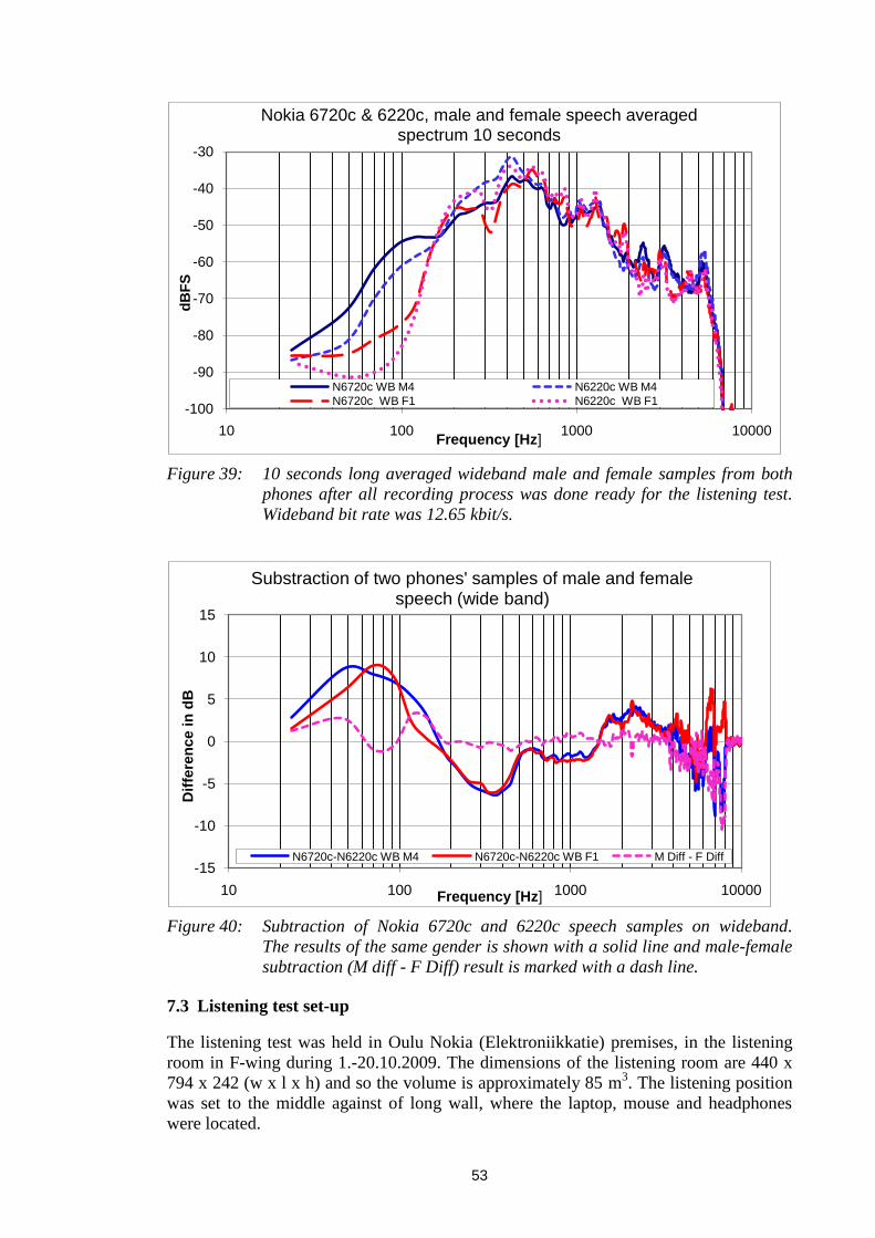
53
Figure 39: 10 seconds long averaged wideband male and female samples from both
phones after all recording process was done ready for the listening test.
Wideband bit rate was 12.65 kbit/s.
Figure 40: Subtraction of Nokia 6720c and 6220c speech samples on wideband.
The results of the same gender is shown with a solid line and male-female
subtraction (M diff - F Diff) result is marked with a dash line.
7.3 Listening test set-up
The listening test was held in Oulu Nokia (Elektroniikkatie) premises, in the listening
room in F-wing during 1.-20.10.2009. The dimensions of the listening room are 440 x
794 x 242 (w x l x h) and so the volume is approximately 85 m3. The listening position
was set to the middle against of long wall, where the laptop, mouse and headphones
were located.
-100
-90
-80
-70
-60
-50
-40
-30
10 100 1000 10000
dB
FS
Frequency [Hz]
Nokia 6720c & 6220c, male and female speech averaged spectrum 10 seconds
N6720c WB M4 N6220c WB M4
N6720c WB F1 N6220c WB F1
-15
-10
-5
0
5
10
15
10 100 1000 10000
Dif
fere
nce i
n d
B
Frequency [Hz]
Substraction of two phones' samples of male and female speech (wide band)
N6720c-N6220c WB M4 N6720c-N6220c WB F1 M Diff - F Diff

54
Figure 41: Listening test position in the listening room.
Since the discrimination skills of the listeners were not known, 2 additional sample
pairs (1 narrowband & 1 wideband) with identical samples were included to the
listening test. There were also 4 sample pairs recorded on the same phone, but on
different volume levels 6/10 and 10/10. These sample pairs recorded on the same phone
volume levels were matched with the loudness tool described in Section 7.2.4. By
looking at the evaluation results of these identical and same phone samples, the skills of
individual listeners were somehow concluded.
7.3.1 Briefing for the listener
In order to get listeners to focus on the desired parameters, short briefing has to be held
before the test. Also, the technical issues were discussed and clarified, like how to use
the test software. If these preparations are skipped, the users may be uncertain how to
interact with the software and the test results may vary a lot depending on the listener.
To avoid any affects on the results just because of lack of information, the following
items were discussed before the test.
Test method
Content of the test
Parameter what listener should evaluate
Possible imperfections that should not affect the evaluations
What is prohibited
Staff location, who to ask if any problems occur
The headphones orientation and position were instructed to the listeners before the test.
Also, the user interface was demonstrated to avoid causing confusion to the listeners.

55
7.3.2 User interface
Because all the listeners and samples were Finnish the user interface language was set to
Finnish. The listening test software was DaGuru and it was run on a normal laptop with
Windows XP operating system.
Using the software was made easy for the listener. First the name and age was given to
the software and after that 8 practicing sample pairs were played. After practicing, the
listener had to listen and rate 50 sample pairs, which took about 30 min. The user had to
listen to a sample pair and grade the recent sample compared to the previous one. When
the sample pair was evaluated, the next pair was played automatically. If a user wanted
to listen to the sample pair again, they were instructed not to use more than 2 repetitions
at save time. The number of evaluated and upcoming samples were on the screen all the
time as can be seen from Figure 42.
Figure 42: User interface in the listening test. Two samples have been played and
the listeners have to choose how good the latest sample is compared to the
previous one. Users can repeat the sample pair by pressing the "Toista"
button.
7.4 Results of the subjective test
After all preparations were done, the subjects took part in the listening test and finally,
the analyzing was proceeded. Altogether 33 subjects took part in the test, from which 17
were male and 16 female. The analyzing process and results of the listening test are
presented in this section.
7.4.1 How the data is analyzed
The analysis of the test results was done on Microsoft excel. DaGuru has an excel add-
on, which reads the listening test data for analyzing. The add-on assorts the answers by
using the first sample as a reference sample and the other as a test sample, which is
evaluated. The Nokia 6220c was selected to be the reference (just in the analyzing
phase) and the grading was executed in the following way: If a listener has given grade
3 to a test sample (Nokia 6720c), the answer is Nokia 6720c grade 3. If the reference
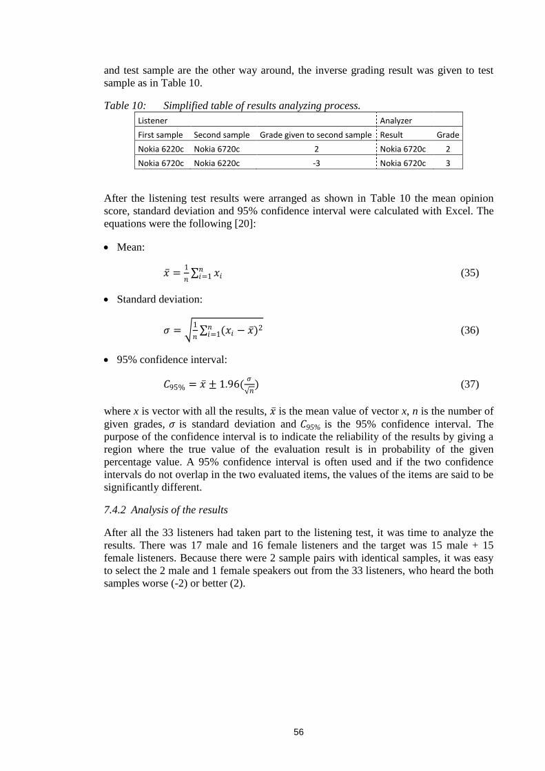
56
and test sample are the other way around, the inverse grading result was given to test
sample as in Table 10.
Table 10: Simplified table of results analyzing process.
Listener Analyzer
First sample Second sample Grade given to second sample Result Grade
Nokia 6220c Nokia 6720c 2 Nokia 6720c 2
Nokia 6720c Nokia 6220c -3 Nokia 6720c 3
After the listening test results were arranged as shown in Table 10 the mean opinion
score, standard deviation and 95% confidence interval were calculated with Excel. The
equations were the following [20]:
Mean:
𝑥 =1
𝑛 𝑥𝑖
𝑛𝑖=1 (35)
Standard deviation:
𝜎 = 1
𝑛 (𝑥𝑖 − 𝑥 )2𝑛
𝑖=1 (36)
95% confidence interval:
𝐶95% = 𝑥 ± 1.96(𝜎
𝑛) (37)
where x is vector with all the results, 𝑥 is the mean value of vector x, n is the number of
given grades, 𝜎 is standard deviation and 𝐶95% is the 95% confidence interval. The
purpose of the confidence interval is to indicate the reliability of the results by giving a
region where the true value of the evaluation result is in probability of the given
percentage value. A 95% confidence interval is often used and if the two confidence
intervals do not overlap in the two evaluated items, the values of the items are said to be
significantly different.
7.4.2 Analysis of the results
After all the 33 listeners had taken part to the listening test, it was time to analyze the
results. There was 17 male and 16 female listeners and the target was 15 male + 15
female listeners. Because there were 2 sample pairs with identical samples, it was easy
to select the 2 male and 1 female speakers out from the 33 listeners, who heard the both
samples worse (-2) or better (2).

57
Figure 43: Means and 95% confidence intervals of all the scores given for the Nokia
6720c compared to the Nokia 6220c. Nominal volume means volume level
6/10 and maximum 10/10. The Nokia 6720c got better scores in every case
evaluated.
When looking at Figure 43 the it should be kept in mind that N6720c has grades from
0.61 to 1.73 and N6220c has thereby inverse grades. It can be noted that male speakers
on wideband benefit significantly more from the large speaker. On the other hand, on
narrowband the benefit from the large speaker is about the same for both male and
female speakers.
In addition to naive and experienced listeners, 7 people from Nokia Oulu
(Teknologiakylä) electro mechanic audio team were invited to the test. The reason for
inviting those 7 people were partly because the listening test arrangements had to be
tested. One other important matter is to obtain information how close the designers
evaluate the test samples compared to the results of other listeners. The results of all
listeners are presented in Figure 44.
N6720c: narrowband
maximum volume
N6720c: narrowband
nominal volume
N6720c: wideband maximum volume
N6720c: wideband nominal volume
Male speaker 1,18 1,58 1,73 1,35
Female speaker 1,03 1,32 0,95 0,61
0,00
0,50
1,00
1,50
2,00
2,50
Gra
de
Means of listeneng test results, CMOS3 & CI95%

58
Figure 44: Means and 95% confidence intervals of all the scores given for the Nokia
6720c compared to the Nokia 6220c. Nominal volume means volume level
6/10 and maximum 10/10.*7 people from Oulu Nokia (teknologiakylä)
electro mechanic audio team took part in the test.
7.5 Discussions about the subjective test
Using the headphones instead of real phones probably affected the test results. Nokia
6220c had audible background noise especially with female narrowband speech, which
may have affected that the Nokia 6720c female speaker narrowband quality was
evaluated better than wideband quality. The standard deviation became fairly large on
narrowband nominal volume among the Nokia audio team listeners, because there was
audible noise in some of the nominal volume listening test files even after noise
reduction. The listeners were instructed not to take the noise into account, but still it has
probably affected the grading. The small population size (7) also has an effect on the
audio team confidence interval.
The processing of the files was an easy task excluding the small noise problem with the
narrowband files. The listening experience could have been better if the loudness
correcting would have been done as the last process before the listening test. A few
listeners said that a couple of files sounded to be at a different volume level, which
could have affected the results.
The listeners said some comments about the darkness of the female sound after the test.
In practice, all the lowest frequencies were produced by the Nokia 6720c. There is a
possibility that low frequencies were emphasized too much for a female speaker and
caused the feeling of dark sound. That may have caused the result that female speaker
audio quality on both phones were almost equally graded, i.e. near zero on wideband.
0,00
0,50
1,00
1,50
2,00
2,50
3,00
N6720c: narrowband maximum volume
N6720c: narrowband nominal volume
N6720c: wideband maximum volume
N6720c: wideband nominal volume
Gra
de
Means of listening test results with Nokia audio group*, CMOS3 & CI95%
Male speaker Female speaker Male speaker, Nokia listener Female speaker, Nokia listener

59
8. CONCLUSIONS
The objective of this thesis was to compare the earpiece integrations in a mobile phone
subjectively. This work contains theory about earpiece integration in mobile phone with
the analysis of objective and subjective measurements. The results of the subjective test
indicate that end-users can distinguish between the different earpiece integrations.
In Chapter 6 the objective measurements were performed and some expectations of
subjective test results were done. The measurements on HATS showed considerable
differences on earpiece integrations. Low frequency reproduction on smaller earpiece
integration was poor due to the earpiece physical limitations discussed in Chapter 5.
In the light of theory and objective measurements, the results of the subjective test were
not a surprise. Male speaker benefit clearly because the low frequencies were produced
much better than the small speaker implementation. Listeners experienced the female
speakers sound as being too dark, but this can be due to recording, processing and using
the headphones for listening to the test files. It was interesting to try how the audio
designers' grades differentiate from normal user listening test results. The Nokia electro
mechanic audio team from Oulu participated in the test with 7 people and graded the
samples with the same trend as the other listeners.
As discussed in Chapter 7, concerning different listening methods, the headphones were
selected to be the most convenient to use for the listener. However, using another
listening method could produce even better grades for larger speaker integration. It
would have been useful to try the listening test with the rapid model under silent and
noisy conditions. The intelligibility test could have been added to the noisy conditions
to see if end-users rate the earpiece integrations the same way as in silent environment.
60
9. REFERENCES
[1] Karjalainen, M. Kommunikaatioakustiikka. Helsinki University of
technology. Laboratory of acoustics and audio signal processing. Report
51. Espoo. 1999. p 237.
[2] Laine, U. S-89.3610 Puheenkäsittely. Helsinki University of technology.
Laboratory of acoustics and audio signal processing. 2006.
[3] Lemmetty, S. Review of Speech Synthesis Technology. Master's thesis.
Helsinki University of Technology. Espoo. 1999. p 113.
[4] Pihlgren, P. Moninopeuksinen puheenkoodaus matkapuhelinverkoissa.
Master's thesis. Helsinki University of Technology. Espoo. 2003. p 123.
[5] ITU-T G.711 standard 10.1.2009 <URL:
http://www.itu.int/rec/dologin_pub.asp?lang=e&id=T-REC-G.711-
198811-I!!PDF-E&type=items>
[6] Suvanen, J. Signal Processing Platform for Multi-Service Networks.
Licentiate work. TKK. 2000.
[7] Rossing, T.D. The Science of Sound. Addison Wesley. 1990.
[8] Alku, P. S-89.3630 Speech transmission technology. Course handout.
TKK. Laboratory of acoustics and audio signal processing. 2008.
[9] Nieminen, T. Floating-Point Adaptive Multi-Rate Speech Codec.
Master's thesis. Tampere University of technology. 2000.
[10] Schroeder, M. Atal, B. Code-excited linear prediction (CELP): high
quality speech at very low bit rates. Proc. IEEE Int. Conf. Acoust.
Speech, Signal Processing. 1984. pp. 937-940.
[11] Suvanen, J. Adaptive Multi-Rate (AMR) Speech Coding. Acoustics and
signal processing seminar. TKK. 1999.
[12] Järvinen, K. Standardisation of the Adaptive Multi-rate Codec. European
Signal Processing Conference (EUSIPCO). Tampere. Finland. 2000.
[13] ETSI ETS 300 726 (GSM 06.60 version 5.2.1). Digital cellular
telecommunications systems, Enhanced Full Rate (EFR) speech
transcoding. (GSM 06.60). 1999.
[14] 3rd Generation Partnership Project: Universal Mobile Telecomminucations
System (UMTS); Mandatory Speech Codec speech processing functions;
AMR speech codec; Transcoding functions. (Release 1999). 3G TS 26.090
version 3.1.0. 2000.
[15] Isherwood, Zacharov & Mattila. NRC subjective test guidelines. Nokia
internal document. 2004.

61
[16] Engberg, A. 8 x 12 Specification Requirements. Nokia internal document.
2009.
[17] Veko, L. Specification requirements for 4.8 x 10 mm. Nokia internal
document. 2007.
[18] Backman, J. S-89.3410 Sähköakustiikka luentomoniste. TKK. Espoo.
2008.
[19] Zacharov, N. Finnish Speech Passages Database. Nokia internal
document. 2005.
[20] Mellin, I.Sovellettu todennäköisyyslasku: Kaavat ja taulukot. Mat-2.091
Sovellettu todennäköisyyslasku course handout. TKK. Espoo. 2003.
[21] Lahti, T. Akustinen mittaustekniikka. Helsinki University of technology,
laboratory of acoustics and audio signal processing. Report 38. Otaniemi.
1997. p 152.
[22] Signaalit ja järjestelmät multimediamateriaalia.
http://130.233.158.46/eopetus/strm-signals/default3.htm. [1.11.2009] TKK
Tietoliikennelaboratorio.
[23] Peltonen, T. A Multichannel Measurement System for Room Acoustics
Analysis. Master of Science Thesis. Helsinki University of
Technology. Laboratory of Acoustics and Audio Signal Processing.
Espoo. 2000. p 119.
[24] Orange press releases. 2009. URL:< http://www.orange.com/
en_EN/press/press_releases/cp090910en.jsp>. [4.11.2009]
[25] Nokia Oyj web site. URL:<http://www.nokia.fi>. [4.11.2009]
[26] 3GPP specification detail. Speech and video telephony
terminal acoustic test specification. TS 26.132. 2008.
URL:<www.3gpp.org>. [10.11.2009]
[27] Tuomela, P. Rakenna hifikaiuttimet. Sanomaprint. 1993. p 202.
[28] Hall, D. Basic acoustics. Krieger publishing company. Florida. 1993. p
345.
[29] Korhonen, P. Comparison of Integrated Hands-Free speaker
technologies. Master's thesis. Helsinki University of technology.
Laboratory of acoustics and audio signal processing. 2002. p 104.
[30] Beranec, L. Acoustics. 1993 Edition. Cambridge. p 491.
[31] Slotte, B. Common acoustic integration guideline for earpieces. Nokia
internal document. 2005.

62
[32] Bessette, B. Salami, R. Lefebvre, R. Jelenek, M. Rotola-Pukkila, J. Vainio,
J. Mikkola, H. Järvinen, K. The Adaptive Multi-Rate Wideband Speech
Codec (AMR-WB). IEEE Transactions on speech and audio processing.
(vol. 10 no.8) 2002. pp. 620-636
[33] 3rd
Generation Partnership Project: Technical Specification Group
Services and System Aspects; Mandatory Speech Codec speech
processing functions; AMR Wideband Speech Codec; Transcoding
Functions. 3GPP TS 26.190 version 1.0.0. 2000.
[34] Mäkinen, K. Tuning of Multiband Dynamic Range Controller for
Integrated Hands-Free Loudspeaker. Master's thesis. Helsinki University
of technology. Laboratory of acoustics and audio signal processing.
2003.
[35] VoiceAge web site. The World's Premier Supplier of Speech and Audio
Codecs. G.722.2 (AMR-WB). URL: <
http://www.voiceage.com/prodamrwb.php> [30.11.2009]
[36] Farina, A. Simultaneous Measurement of Impulse Response and Distortion
with a Swept-Sine Technique. AES 108th
convention. Paris. Preprint
No. 5093 (D-4). 2000. p 23.
[37] R&S CMU200 Universal Radio Communication Tester. Data sheet.
Version 08.01. 2007.

63
10. APPENDICES
APPENDIX A: Large speaker used in Nokia 6720c mobile phone
Figure 45: Large speaker dimensions used in Nokia mobile phone in listening test.
The dimensions are taken from [16].
Figure 46: Measures of the large speaker membrane used in Nokia mobile phone
in listening test.

64
APPENDIX B: Small speaker used in Nokia 6220c mobile phone
Figure 47: Small speaker dimensions used in Nokia mobile phone in listening test.
Dimensions are taken from [17].
Figure 48: Membrane measures of small speaker used in Nokia mobile phone in
listening test.

65
APPENDIX C: Listening test instructions (in Finnish)
Kuuntelukoeohje
Tässä kuuntelukokeessa kuunnellaan suomenkielisiä puhelinääninäytteitä. Näytteet
soitetaan pareittain, joista arvioidaan jälkimmäisenä kuultua näytettä verrattuna
ensimmäiseen asteikolla -3 (Paljon huonompi)…3 (Paljon parempi). Jos jälkimmäinen
on mielestäsi huonompi kuin ensimmäinen, valitse -3…-1. Jälkimmäisen ollessa
parempi kuin ensimmäinen, valitse 1...3. Jos et kuule eroa näytteiden välillä, valitse 0.
Arvioinnin perusteena on, kumpi näytteistä kuulostaa mielestäsi paremmalta.
Äänenvoimakkuus säädetään testin alussa kuuntelijalle sopivaksi, eikä sitä tarvitse
muuttaa testin aikana. Jos haluat kuulla näyteparin uudelleen, voit toistaa sen
enimmillään 2 kertaa, jottei testi mene liian pitkäksi.
Kun kuuntelukoe alkaa, ohjelma kysyy nimeäsi ja ikääsi. Voit kirjoittaa sen muodossa
NimiS 15V, jossa S on sukunimen ensimmäinen kirjain. Aluksi kuunnellaan 8
harjoitusnäyteparia, jonka jälkeen varsinainen testi alkaa. Tämän jälkeen kuunnellaan
25 paria nykyisin puhelimissa kuultavaa puhelinääntä, joiden jälkeen tulee 25 paria
tulevasta laajakaistaisesta puhelinäänestä.
Joissakin näytteissä voi olla häiriöitä (epäjatkuvuus, kohina), joita ei tarvitse huomioida
näytettä arvioidessa.
Laitathan kännykän äänettömälle testin ajaksi.
Jos kokeen aikana tulee kysyttävää, voit soittaa Sampalle 0440321069.

66
APPENDIX D: Matlab code for 7.8 khz filter
% 8kHz lowpass filter parameters (FIR equiripple)
% All frequency values are in Hz. Fs = 48000; % Sampling Frequency Fpass = 7700; % Passband Frequency Fstop = 8300; % Stopband Frequency Dpass = 0.057501127785; % Passband Ripple Dstop = 0.001; % Stopband Attenuation dens = 20; % Density Factor % Calculate the order from the parameters using FIRPMORD. [N, Fo, Ao, W] = firpmord([Fpass, Fstop]/(Fs/2), [1 0], [Dpass, Dstop]); % Calculate the coefficients using the FIRPM function. b = firpm(N, Fo, Ao, W, {dens}); % Sound file is read [x, fs, nbits] = wavread('input_file.wav'); % Sound file is filtered using filter specs above y = filter(b,1,x); % The frequency response of original sound file is calculated xF = 20*log10(abs(fft(x))); % The frequency response of original sound file is plotted figure(2); plot(xF,'g');
% Hold is done to plot both curves to same figure hold on; % The frequency response of filtered sound file is calculated yF = 20*log10(abs(fft(y))); % The frequency response of filtered sound file is plotted plot(yF,'r'); % Filtered sound file is written to hard drive wavwrite(y,Fs,nbits,'output_file');

67
APPENDIX E: Matlab code for 5.5 khz lowpass filter
% 5,5kHz lowpass filter parameters. % All frequency values are in Hz.
Fs = 48000; % Sampling Frequency Fpass = 5500; % Passband Frequency Fstop = 6400; % Stopband Frequency Dpass = 0.057501127785; % Passband Ripple Dstop = 0.001; % Stopband Attenuation dens = 20; % Density Factor % Calculate the order from the parameters using FIRPMORD. [N, Fo, Ao, W] = firpmord([Fpass, Fstop]/(Fs/2), [1 0], [Dpass, Dstop]); % Calculate the coefficients using the FIRPM function. b = firpm(N, Fo, Ao, W, {dens}); % Sound file is read [x, fs, nbits] = wavread('input_file.wav'); % Sound file is filtered using filter specs above y = filter(b,1,x); % The frequency response of original sound file is calculated xF = 20*log10(abs(fft(x))); % the frequency response of original sound file is plotted figure(2); plot(xF,'g'); hold on; % the frequency response of filtered sound file is calculated yF = 20*log10(abs(fft(y))); % the frequency response of filtered sound file is plotted plot(yF,'r'); % Filtered sound file is written to hard drive wavwrite(y,Fs,nbits,'output_file');
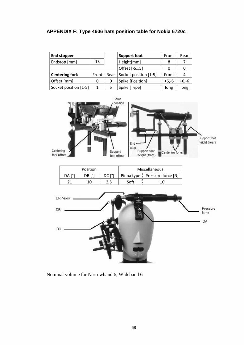
68
APPENDIX F: Type 4606 hats position table for Nokia 6720c
End stopper Support foot Front Rear
Endstop [mm] 13
Height[mm] 8 7
Offset [-5…5] 0 0
Centering fork Front Rear Socket position [1-5] Front 4
Offset [mm] 0 0 Spike [Position] +6,-6 +6,-6
Socket position [1-5] 1 5 Spike [Type] long long
Position Miscellaneous
DA [°] DB [°] DC [°] Pinna type Pressure force [N]
21 10 2,5 Soft 10
Nominal volume for Narrowband 6, Wideband 6

69
APPENDIX G: Type 4606 hats position table for Nokia 6220c
End stopper Support foot Front Rear
Endstop [mm] 16
Height[mm] 8 8
Offset [-5…5] 0 0
Centering fork Front Rear Socket position [1-5] Front 4
Offset [mm] 0 0 Spike [Position] +6,-6 +6,-6
Socket position [1-5] 2 3 Spike [Type] long long
Position Miscellaneous
DA [°] DB [°] DC [°] Pinna type Pressure force [N]
21 10 -2 Soft 10
Nominal volume for Narrowband 5, Wideband 4