Subdivision surface fitting for efficient compression and coding of 3D models

Guillaume Lavoué*, Florent Dupont and Atilla Baskurt

LIRIS UMR 5205 CNRS, 43, Bd du 11 novembre, 69622 Villeurbanne Cedex, France

ABSTRACT

In this paper we present a new framework, based on subdivision surface fitting, for high rate compression and coding of 3D models. Our algorithm fits the input 3D model, represented by a polygonal mesh, with a piecewise smooth subdivision surface represented by a coarse control polyhedron. Our fitting scheme, particularly suited for meshes issued from mechanical or CAD parts, aims at getting close to the optimality in terms of control points number, while remaining independent of the connectivity of the input mesh. The found subdivision control polyhedron is much more compact than the original mesh and visually represents the same shape after several subdivision steps, without artifacts or cracks, like traditional lossy compression schemes. This control polyhedron is then encoded specifically to give the final compressed stream. Experiments conducted on several 3D models have proven the coherency and the efficiency of our framework, compared with existing compression methods.

Keywords: CAD mesh, Compression, Visualization, Approximation, Subdivision surface.

1. INTRODUCTION AND CONTEXT Advances in computer speed, memory capacity, and hardware graphics acceleration have highly increased the amount of three-dimensional models being manipulated, visualized and transmitted over the Internet. In this context, the need for efficient tools to retrieve, protect or reduce the storage of this 3D content, mostly represented by polygonal meshes, becomes even more acute. The context of our work is the SEMANTIC-3D project (http://www.semantic-3d.net) of which the principal issue is the transmission of 3D mechanical models through low bandwidth channels in a visualization objective on various terminals. The 3D model database to handle comes from the car manufacturer Renault, and contains thousands of quite irregular polygonal meshes representing CAD parts. Thus an efficient compression tool is needed to reduce the amount of data carried by this 3D content, knowing that the original NURBS information is not available. Many efficient techniques have been developed for encoding polygonal meshes1,2,3 but fundamentally, this representation remains very heavy in terms of amount of data (a large points set, on top of the connectivity has to be encoded). Moreover, lossy compression schemes like wavelet based ones4,5 produce artifacts, visually damaging for piecewise smooth mechanical objects. Other models exist to represent a 3D shape: NURBS surfaces or subdivision surfaces. These models are much more compact. A subdivision surface is a smooth (or piecewise smooth) surface defined as the limit surface generated by an infinite number of refinement operations using a subdivision rule on an input coarse control mesh. Hence, it can model a smooth surface of arbitrary topology (contrary to a NURBS model which needs a parametric domain) while keeping a compact storage and a simple representation (a polygonal mesh). Moreover it can be easily displayed to any resolution. Subdivision surfaces are now widely used for 3D imaging and have been integrated to the MPEG4 standard6. For all these reasons, we have developed a new algorithm, based on subdivision surface fitting for efficiently compressing 3D meshes, for low bandwidth transmission and storage. The 3D models are first approximated by piecewise smooth subdivision surfaces, associated with control polyhedrons which are then encoded specifically to give the compressed bit stream. Hence the 3D model, once approximated, will be transmitted in the form of an encoded coarse polyhedron and, at the reception, displayed to any resolution, according to the terminal capacity, by iterative subdivisions. Note that this decompression process is very simple and therefore adapted for mobile terminals. Section 2 details the related work about mesh compression and subdivision surface fitting, while the overview of our method and the prior work are presented in section 3. Sections 4 and 5 detail the two steps of our subdivision surface fitting approach: the initialization and the optimization of the subdivision surfaces. Finally section 6 presents the final control mesh construction and encoding, and the results of our experiments. * glavoue@liris.cnrs.fr, phone (33) 4 72 44 83 95, fax (33) 4 72 43 15 36, http://liris.cnrs.fr/guillaume.lavoue

2. RELATED WORK

2.1. Mesh compression A lot of work has been done about polygonal mesh compression. This representation contains two kinds of information: geometry and connectivity, the first describing coordinates of the vertices in the 3D space, and the later describing how to connect these positions. The connectivity graph is often encoded using a region growing approach based on faces2, edges3 or vertices1. Others techniques consider progressive approaches which encode a base mesh and then vertex insertion operations7. Fewer efforts have been done about geometry compression which is often simply performed by predictive coding and quantization. Other researches have put more efforts on geometry driven mesh coding, using wavelets4,5 or spectral compression8. On the whole, better mesh compression methods give between 1 and 2 bytes per vertex; although this represents an excellent result, the output bit stream remains large for complex objects because of the high number of vertices to encode. Moreover lossy compression schemes4,5,7,8 often produce artifacts, visually damaging for smooth mechanical objects. That is why we have chosen to approximate input meshes with subdivision surfaces, of which control polyhedrons should contain much lesser faces to store or transmit, knowing that after several refinement steps, the subdivision surfaces will visually represent the shape of the original meshes (of which original connectivity will not be kept).

2.2. Subdivision surface approximation Several methods already exist for subdivision surface fitting, most of them take as input a dense mesh, simplify it to obtain a base coarse control mesh9,10 and then displace the control points (geometry optimization) to fit the target surface. These simplification based approaches allow to easily extract a control mesh with the same topology than the target object, however, the control mesh connectivity strongly depends on the input mesh and therefore can give quite bad results if the input mesh is very irregular, which is the case for our CAD models. Hence, in our algorithm, in order to remain independent of the original connectivity, we first decompose the object into surface patches, and then we use the boundaries of the patches and the curvature information to construct a control polyhedron having the same topology than the target object. Some algorithms11,12 also remain independent of the target mesh, by iteratively subdividing and shrinking an initial control mesh toward the target surface. Unfortunately these methods fail to capture local characteristics for complex target surfaces. Once a coarse control mesh has been constructed, then the geometry has to be optimized by moving control points to match the subdivision surface with the target model. Lee et al.9 and Hoppe et al.13 sample a set of points from the original mesh and minimize a quadratic error to the subdivision surface. Suzuki et al.11 propose a faster approach, also used in Ref. 12: the position of the control points is optimized, only by reducing the distances between their limit positions and the target surface. Hence only subsets of the surfaces are involved on the fitting procedure, thus results are not so precise and may produce oscillations. Ma et al.10 consider the minimization of the distances from vertices of the subdivision surface after several refinements, to the target mesh; our algorithm follows this framework while using not a point to point distance minimization, but a point to surface minimization, by using the local quadratic approximants introduced by Pottmann and Leopoldseder14. This algorithm allows a more accurate and rapid convergence. To our knowledge, the optimality in terms of control points number and connectivity of the control polyhedron represents a minor problematic in the existing algorithms but seems particularly relevant for mechanical or CAD objects. Only Hoppe et al.13 optimize the connectivity (but not the number of control points) by trying to collapse, split, or swap each edge of the control polyhedron. Their algorithm produces high quality models but need of course an extensive computing time. Our algorithm optimizes the connectivity of the control mesh by analyzing curvature directions of the target surface, which reflect the natural parameterization of the object. The number of control points is also optimized by enriching iteratively the control polyhedron according to the error distribution. Moreover our approach allows to directly control the approximation error, whereas simplification based methods9,10 indirectly control the error by modifying the decimation level.

3. OVERVIEW OF OUR ALGORITHM AND PRIOR WORK

3.1. Overview Our framework for compression of 3D models is the following: Firstly the target 3D objects are segmented into surface patches (see Section 3.4), of which boundaries are extracted. Secondly, the network of boundaries is approximated with piecewise smooth subdivision curves (see Sections 3.3 and 3.5); this step provides a network of control polygons.

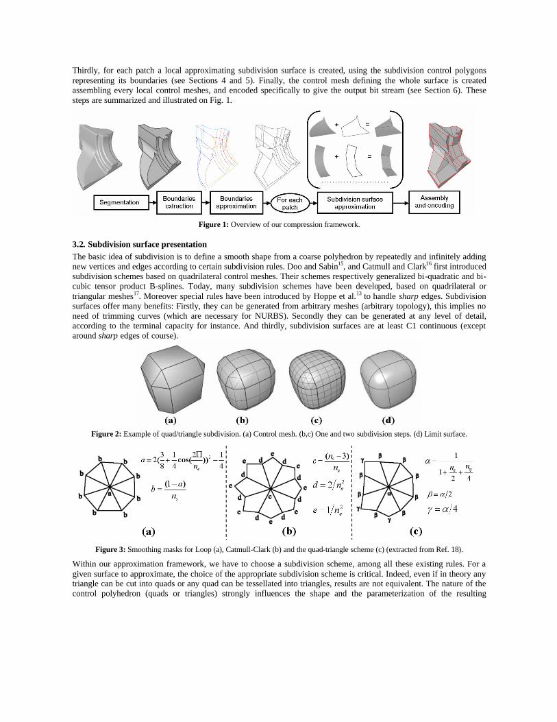
Thirdly, for each patch a local approximating subdivision surface is created, using the subdivision control polygons representing its boundaries (see Sections 4 and 5). Finally, the control mesh defining the whole surface is created assembling every local control meshes, and encoded specifically to give the output bit stream (see Section 6). These steps are summarized and illustrated on Fig. 1.

Figure 1: Overview of our compression framework.

3.2. Subdivision surface presentation The basic idea of subdivision is to define a smooth shape from a coarse polyhedron by repeatedly and infinitely adding new vertices and edges according to certain subdivision rules. Doo and Sabin15, and Catmull and Clark16 first introduced subdivision schemes based on quadrilateral control meshes. Their schemes respectively generalized bi-quadratic and bi-cubic tensor product B-splines. Today, many subdivision schemes have been developed, based on quadrilateral or triangular meshes17. Moreover special rules have been introduced by Hoppe et al.13 to handle sharp edges. Subdivision surfaces offer many benefits: Firstly, they can be generated from arbitrary meshes (arbitrary topology), this implies no need of trimming curves (which are necessary for NURBS). Secondly they can be generated at any level of detail, according to the terminal capacity for instance. And thirdly, subdivision surfaces are at least C1 continuous (except around sharp edges of course).

Figure 2: Example of quad/triangle subdivision. (a) Control mesh. (b,c) One and two subdivision steps. (d) Limit surface.

Figure 3: Smoothing masks for Loop (a), Catmull-Clark (b) and the quad-triangle scheme (c) (extracted from Ref. 18).

Within our approximation framework, we have to choose a subdivision scheme, among all these existing rules. For a given surface to approximate, the choice of the appropriate subdivision scheme is critical. Indeed, even if in theory any triangle can be cut into quads or any quad can be tessellated into triangles, results are not equivalent. The nature of the control polyhedron (quads or triangles) strongly influences the shape and the parameterization of the resulting

subdivision surface. The body of the cylinder, for instance, is much more naturally parameterized by quads than by triangles. These reasons have led us to choose the hybrid quad/triangle scheme developed by Stam and Loop18. This scheme reproduces Catmull-Clark on quad regions and Loop on triangle regions. At each subdivision step, the base mesh is firstly linearly subdivided: Each edge is splitted into two, each triangle into four and each quad into four (see Figure 2). Secondly, each vertex is replaced by a linear combination of itself and its direct neighbors. When a vertex is entirely surrounded by triangles or quads we use smoothing masks of Figure 3.a and Figure 3.b and otherwise we use the mask from Figure 3.c, which depends on the numbers of edges ne and quads nq surrounding the vertex.

3.3. Subdivision curve presentation A subdivision curve is created using iterative subdivisions of a control polygon. In this paper we use the subdivision rules defined for surfaces by Hoppe et al.13 for the particular case of sharp or boundary edges: New vertices are inserted at the midpoints of the control segments and new positions Pi' for the control points Pi are computed using their old values and those of their two neighbors using the mask:

)PPP(P iiii 11 681

+− +×+=′ (1)

We also consider specific rules (those defined by Hoppe et al.13 for corner vertices) to handle sharp parts and extremities: Pi’ = Pi. This subdivision curve will coincide with the boundary generated by commonly used subdivision surface rules like Catmull-Clark16, Loop17 or the quad-triangle scheme from Stam and Loop18.

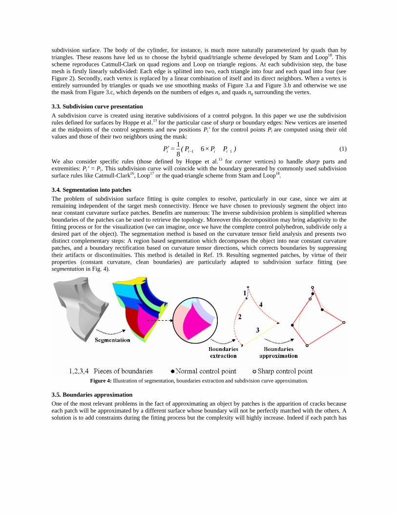
3.4. Segmentation into patches The problem of subdivision surface fitting is quite complex to resolve, particularly in our case, since we aim at remaining independent of the target mesh connectivity. Hence we have chosen to previously segment the object into near constant curvature surface patches. Benefits are numerous: The inverse subdivision problem is simplified whereas boundaries of the patches can be used to retrieve the topology. Moreover this decomposition may bring adaptivity to the fitting process or for the visualization (we can imagine, once we have the complete control polyhedron, subdivide only a desired part of the object). The segmentation method is based on the curvature tensor field analysis and presents two distinct complementary steps: A region based segmentation which decomposes the object into near constant curvature patches, and a boundary rectification based on curvature tensor directions, which corrects boundaries by suppressing their artifacts or discontinuities. This method is detailed in Ref. 19. Resulting segmented patches, by virtue of their properties (constant curvature, clean boundaries) are particularly adapted to subdivision surface fitting (see segmentation in Fig. 4).

Figure 4: Illustration of segmentation, boundaries extraction and subdivision curve approximation.

3.5. Boundaries approximation One of the most relevant problems in the fact of approximating an object by patches is the apparition of cracks because each patch will be approximated by a different surface whose boundary will not be perfectly matched with the others. A solution is to add constraints during the fitting process but the complexity will highly increase. Indeed if each patch has

constraints with its neighbors, the algorithm will become a global optimization problem. Another solution is to treat these cracks after the fitting process but the approximating surfaces will be modified, compared with the first approximation. Our solution is simpler and more effective. The subdivision surface approximation problem is divided into two sub-problems: The piecewise approximation of the boundaries of the patches and the construction of the final subdivision surfaces by interpolation of the found boundaries and approximation of the interior data. Accordingly, for each patch the boundary is divided into pieces of boundary corresponding to the different adjacencies with its neighboring regions (see Boundaries extraction in Fig. 4). Then the pieces of boundary are approximated with subdivision curves following our algorithm described in Ref. 20, which are then glued together (see Boundaries approximation in Fig. 4). According to subdivision properties, the associated control polygon will represent the boundary of the control polyhedron of the approximating subdivision surface. Then, for each patch, our process will attempt to connect control points of the control polygon, to create the initial control polyhedron.

4. LOCAL SUBDIVISION SURFACE INITIALIZATION

4.1. Principle Considering a surface patch, once the control polygon representing its boundary has been constructed, the purpose is to create edges and facets by connecting these control points. For this purpose, we consider the lines of curvature of the original surface, represented by local directions of minimum and maximum curvature. Control lines of a subdivision surface are strongly linked to the lines of curvature. Indeed the topology of a control polyhedron will strongly influence the geometry information of the associated limit surface, which is also carried by lines of curvature21. This coherency between control lines and lines of curvature is shown in the example on Figure 5.

Figure 5: The coherency between control lines (a), minimum (b) and maximum (c) directions of curvatures.

Figure 6: Mechanism for edge score definition.

Thus, for each couple of control points from the boundary control polygon, a Coherency Score (SC) is calculated, taking into account the coherency of the corresponding potential control edge with the lines of curvature of the corresponding area on the target surface. The mechanism is illustrated on Figure 6: For each potential edge E, we consider its vertices

P0, P1 and their respective limit positions ∞0P , ∞

1P . Then we calculate the pseudo geodesic path between these limit

positions, to simulate the control line, by applying the Dijkstra algorithm on the vertices of the original surface. Finally we consider the curvature tensors of the n vertices Vi of this path, and particularly their curvature directions. The coherency score SC for this potential edge E is:

n

)max,minmin()E(SC

n

i in

i i ∑∑ === 11θθ

(2)

where iminθ (resp. imaxθ ) is the angle between the minimum (resp. maximum) curvature direction of the vertex Vi

and the segment ∞0P ∞

1P . This score SC ∈[0,90] is homogeneous to an angle value in degrees.

4.2. Algorithm Our algorithm is the following: At each iteration, we consider the potential edge associated with the smallest score SC (dotted segments in Figure7.b) and we cut the boundary control polygon along this edge. This operation is repeated until it remains only plane polygons. Then for each of them, we check its convexity; if it is convex, we create a facet, and if not, we decompose it into convex parts. By assembling created facets we obtain our initial control polyhedron (see Figure 7.c) of which limit surface (see Figure 7.d) represents in most case a quite good approximation of the original surface (see Figure 7.a).

Figure7: Example of local subdivision surface initialization.

5. LOCAL SUBDIVISION SURFACE OPTIMIZATION The initial subdivision surface often represents a sufficient approximation of the target surface patch, even if the initialization process considers first of all the boundary information. Indeed, owing to the curvature based segmentation step, surface patches are quite simple surfaces, of which most of the geometry information is carried by the boundaries. However, in some cases some more control points may be needed to correctly approximate the target shape. Considering this purpose, we have defined two complementary mechanisms: An enrichment mechanism which adds points and optimizes the connectivity according to the error position and distribution, and a geometry optimization algorithm, generalizing Pottmann and Leopoldseder method14 for the complex quad-triangle subdivision rules.

5.1. Enrichment and connectivity optimization In this section we present how to modify and optimize the connectivity of our control polyhedron. We have two mechanisms to consider: An enrichment of the mesh, consisting in the addition of new control points, and an optimization of the connectivity, insuring that, for a given set of control points, the associated connectivity (set of faces and edges) is the better possible regarding to the resulting error. This mechanism is quite complex to implement, therefore, since the connectivity has been optimized in the initialization step, we will just try to limit its departure. Hence we have integrated these two mechanisms into a single algorithm, which considers the error distribution to enrich precisely the polyhedron, while trying to keep a near optimal connectivity. Considering a target surface and a corresponding initial subdivision surface, the first step of this algorithm is the principal error field extraction. The goal is to extract not only the maximum error point but an area (a set of error points) corresponding to the error field in order to be able to analyze the error distribution. For this purpose we consider sample points Sk, on the subdivision surface and associated distances dk to the corresponding projections on the target surface.

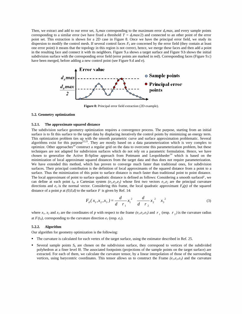
Then, we extract and add to our error set, Skmax corresponding to the maximum error dkmax, and every sample points corresponding to a similar error (we have fixed a threshold T = dkmax/2) and connected to an other point of the error point set. This extraction is shown for a 2D case in Figure 8. Once we have the principal error field, we study its dispersion to modify the control mesh. If several control faces Fk are concerned by the error field (they contain at least one error point) it means that the topology in this region is not correct, hence, we merge these faces and then add a point in the resulting face and connect it with its neighbors. Figure 9.a shows a target surface and Figure 9.b shows the initial subdivision surface with the corresponding error field (error points are marked in red). Corresponding faces (Figure 9.c) have been merged, before adding a new control point (see Figure 9.d and e).

Figure 8: Principal error field extraction (2D example).

5.2. Geometry optimization

5.2.1. The approximate squared distance The subdivision surface geometry optimization requires a convergence process. The purpose, starting from an initial surface is to fit this surface to the target data by displacing iteratively the control points by minimizing an energy term. This optimization problem ties up with the smooth parametric curve and surface approximation problematic. Several algorithms exist for this purpose22,23. They are mostly based on a data parameterization which is very complex to optimize. Other approaches24 construct a regular grid on the data to overcome this parameterization problem, but these techniques are not adapted for subdivision surfaces which do not rely on a parametric formulation. Hence, we have chosen to generalize the Active B-Spline approach from Pottmann and Leopoldseder14 which is based on the minimization of local approximate squared distances from the target data and thus does not require parameterization. We have extended this method, which has proven to converge much faster than traditional ones, for subdivision surfaces. Their principal contribution is the definition of local approximants of the squared distance from a point to a surface. Thus the minimization of this point to surface distance is much faster than traditional point to point distance. The local approximant of point to surface quadratic distance is defined as follows: Considering a smooth surfaceΦ, we can define at each point t0, a Cartesian system (e1,e2,e3) whose first two vectors e1,e2 are the principal curvature directions and e3 is the normal vector. Considering this frame, the local quadratic approximant Fd(p) of the squared distance of a point p at (0,0,d) to the surface Φ is given by Ref. 14:

23

22

2

21

1321 xx

dd

xd

d)x,x,x(Fd +

++

+=

ρρ (3)

where x1, x2 and x3 are the coordinates of p with respect to the frame (e1,e2,e3) and 1ρ (resp. 2ρ ) is the curvature radius at Φ(t0), corresponding to the curvature direction e1 (resp. e2).

5.2.2. Algorithm Our algorithm for geometry optimization is the following:

§ The curvature is calculated for each vertex of the target surface, using the estimator described in Ref. 25.

§ Several sample points Sk are chosen on the subdivision surface, they correspond to vertices of the subdivided polyhedron at a finer level l0. The associated footpoints (projections of the sample points on the target surface) are extracted. For each of them, we calculate the curvature tensor, by a linear interpolation of those of the surrounding vertices, using barycentric coordinates. This tensor allows us to construct the Frame (e1,e2,e3) and the curvature

radiuses 1ρ and 2ρ , useful for the point to surface distance computation (see Equation 3). Sample points Sk can be

computed as linear combinations of the initial control points 0iP (see Section 3.2); they correspond to control points

0liP at the finer level l0.

)P,...,P,P(CS nkk00

20

1= (4) The functionals Ck are determined using iterative multiplications of the l0 subdivision matrices Ml associated with our subdivision rules, which give the new positions of control points according to the old ones. These subdivision matrices Ml are such as 1−×= l

ll PMP with Tl

nlll )]P,...P,P[(P 21= . Thus the functionals Ck for the level l0, are

the lines of the matrix C such as:

∏=

×=0

01

l

lll LMC (5)

0lL is the limit matrix which gives the limit positions, proposed by Stam and Loop18, of the considered control

points at the level l0.

§ For all Sk, local quadratic approximants kdF of the squared distances to the target surface are expressed according to

the frames (e1,e2,e3) at the corresponding Footpoints. The minimization of their sum F gives the new positions of the

control points 0iP .

∑∑ ==k

nkk

dk

kk

d ))P,...,P,P(C(F)S(FF 002

01 (6)

The minimization of this quadratic function leads to the resolution of a linear squared system. Concerning the choice of the number of sample points Sk , we have chosen l0=2 refinements for all examples in this article. As for each refinement, the number of vertices will increase by a factor of at least four, the number of equations will be about sixteen times the number of unknowns. That ensures a stable solution when solving equation (6) in the least squares sense. This algorithm provides a very fast convergence, which is critical since this geometry optimization is a computationally costly procedure.

Figure 9: Connectivity and geometry optimization example. (a) Original surface. Initial (b,c), enriched (d,e) and optimized

(geometry) (f,g) subdivision surface.

5.3. Whole optimization algorithm Our algorithm for the optimization of local subdivision surfaces is the following: Begin Subdivision Surface Optimization

While (E>ELimit) // E is the approximation error and ELimit a threshold value. While (E>ELimit and m<m0)

// m is the geometry optimization iteration number and m0 a maximum number. Call the geometry optimization procedure (see Section 5.2). The subdivision surface is moved toward the target surface, by minimizing a sum of quadratic distances.

End While If (E>ELimit)

A new control point is inserted onto the subdivision surface according to the error distribution (see Section 5.1).

End If End While

End Subdivision Surface Optimization

m0 was fixed to 5, in order to limit the number of iterations for the geometry optimization, since its convergence is very fast (often 3 or 4 iterations) and seeing that this process remains computationally costly. Note that boundary control points are fixed, to insure that no crack will appear later, during the construction of the final whole control polyhedron containing every control meshes of the different patches. Figure 9 shows the complete process. Boundaries of the target surface (see Figure 9.a) have been approximated and an initial subdivision surface has been constructed (see Fig. 9.b) associated with a control polyhedron (see Fig. 9.c). The associated approximation L1 error is E=30.7×10-3. Then the error distribution is analyzed and corresponding faces are merged. A new point in inserted (see Figure 9.d and 9.e) and the surface geometry is optimized (3 iterations) (see Figure 9.f and 9.g). The final approximation error is E=5.8×10-3. 6. CONSTRUCTION AND CODING OF THE FINAL CONTROL POLYHEDRON AND RESULTS

6.1. Encoding Once each patch has been fitted with a subdivision surface, the final control polyhedron for the whole object is created by assembling local control polyhedrons while marking local boundary control edges as sharp (specific subdivision rules which respect sharpness of the edges). This control polyhedron containing triangles, quadrangles, higher order polygons and marked edges is then encoded. Concerning connectivity information, we have chosen to implement the Face Fixer3 algorithm seeing that this encoding scheme is based on edges and allows to process arbitrary polygonal meshes and not just fully triangulated ones. In addition this scheme, which provides quite good compression rates, is able to encode easily face groupings which can be useful, in a perspective way, to transmit the segmentation results within the object. This algorithm encodes the connectivity graph by a list of n labels among k (k~10, depending on the maximum face degree), with n the number of edges. The corresponding bit stream is created using an arithmetic coder which achieves quite good results. Concerning geometry encoding, a 10 bit quantization is performed. Then we eliminate some coordinates, indeed, once the positions of three vertices of a planar face are known, we have to encode only 2 coordinates for the remaining vertices. Flags on the edges (sharp or not) are represented by a n sized binary vector, encoded by a run length algorithm. Thus the total size of the compressed stream is the sum of the connectivity (C), geometry (G) and flags (F) sizes (see examples in Fig. 10, C, G and F are given in bytes).

6.2. Results and discussions Our compression scheme was tested on the mechanical database from Renault, these models are issued from CAD, and thus associated with highly irregular connectivity (see mesh examples on Figure 11). Figure 10 presents the results for the Fandisk mesh (Figure 10.a) and for several objects from Renault database. All these experiments were conducted on a PC, with a 2Ghz XEON bi-processor; processing times are between 5 and 10 seconds for the whole compression

process (the decompression is instantaneous). The models have been scaled in a bounding box of length equal to 1. Figure 10 shows initial objects (with patch boundaries in green), control polyhedrons and associated limit surfaces while detailing the number of vertices and faces of the original objects and of the corresponding control polyhedrons. Original and compressed sizes, in bytes, are also highlighted. Control polyhedrons have widely less faces and vertices compared with initial surfaces and the approximation errors remain very low (limit surfaces are very close from original objects). Mean L1, L2 and maximum errors are shown on Table I, they are calculated between the original object and the subdivision surface after 4 refinement steps. Table I shows original binary sizes (BS), sizes of these binary files compressed with the Zip coder (ZIP) and associated compression rates (ZIP CR). Although the ZIP coder is lossless without any quantization, these values can be compared with compressed file sizes (CS) obtained with our compression algorithm, which achieves extremely high compression rates (CR=BS/CS).

Figure 10: Results of our fitting scheme for different mechanical parts. Initial objects (patch boundaries are marked in green), control polyhedrons (sharp edges are marked in red), and limit surfaces.

Figure 11: Examples of mesh connectivity of our 3D model database and corresponding letters on Figure 10.

Table I: Original binary sizes (BS), Zipped binary sizes (ZIP) and associated rate (ZIP CR). Compressed size (CS) with our algorithm, associated compression rates (CR) and associated L1, L2 and maximum errors.

BS (Bytes)

ZIP (Bytes)

ZIP CR CS (bytes)

CR L1 Error (10-3)

L2 Error (10-3)

Max Error (10-3)

Fig10.a 233 772 59 438 3.93 292 801 0.887 0.012 10.18 Fig10.b 45324 5420 8.36 287 158 0.664 0.006 7.17 Fig10.c 98 748 29 680 3.33 183 540 0.985 0.014 5.94 Fig10.d 156 708 16 849 9.30 192 816 0.765 0.011 7.31 Fig10.e 298 608 45 539 6.56 208 1436 2.588 0.043 21.66 Fig10.f 80 784 12 014 6.72 387 209 0.953 0.012 33.09

Table II shows a comparison, for the Fandisk object, with different state of the art algorithms: Alliez and Desbrun progressive encoding [8] and the wavelets based algorithms from Khodakovsky et al. [4] and Valette and Prost [5]. Our algorithm achieves drastically better compression rates (~800), while keeping a low geometric error. Coders from Alliez and Valette are presented in their lossless versions, thus the geometric error is limited to the quantization error QE (a 10 bits quantization, like ours).

Table II: Compressed sizes, associated compression rates and L2 errors for several compression algorithms applied to Fandisk.

Alliez at al. [8] Valette and Prost [5]

Khodakovsky et al. [4]

Our scheme

Size (bytes) 14 075 10 603 6 063 292 CR 17 22 39 801

L2 Error (10-3) QE QE 0.045 0.012

Results are also particularly suited for our visualization task; indeed, resulting surfaces after subdivision are quite smooth and visually pleasant, without discontinuities or noise like those produced by lossy compression schemes like wavelet based ones for instance. Particularly, our algorithm, thanks to the segmentation step, preserves sharp features.

7. CONCLUSION

We have presented a new framework for compression and coding of 3D models. Our approach is based on subdivision surface approximation and is particularly adapted for mechanical or CAD objects. The approximation algorithm aims at optimizing the connectivity and the control points number of the generated subdivision surface, while remaining independent of the original mesh connectivity. After a segmentation step, the 3D object is decomposed into surface patches of which boundaries are approximated with subdivision curves. Then initial local subdivision control polyhedrons are created by linking control points of the boundary control polygons. These edges are created with respect to the lines of curvature, to preserve the natural parameterization of the target object. Local subdivision surfaces are then iteratively enriched and optimized until the approximation errors become correct. The final whole control polyhedron containing triangles, quadrangles, higher order polygons and sharp edges is then created by assembling local subdivision control polyhedrons, and encoded using an efficient edge based algorithm followed by an entropic coding for the connectivity and a 10 bit quantization for the geometry. Results show quite impressive compression rates compared with state of the art algorithms. Thanks to subdivision properties, at the decompression step, the object can be displayed at any resolution, according to the terminal capacity for example. Moreover limit surfaces are visually pleasant (at least C0 and piecewise C1), without artifacts or cracks, like traditional lossy compression schemes, and sharp features of the original models are preserved. Our method is effective for mechanical models since they present large constant curvature regions which are particularly adapted for subdivision inversion. On the other hand, our method is less suited for natural objects. Concerning perspectives, we plan to improve the connectivity optimization during mesh enrichments, by conducting a deeper analysis of the error dispersion. Finding a way to treat natural noisy objects is also of interest.

ACKNOWLEDGEMENTS

This work is supported by the French Research Ministry and the RNRT (Réseau National de Recherche en Télécommunications) within the framework of the Semantic-3D national project (http://www.semantic-3d.net).

REFERENCES

1. C. Touma, C. Gotsman, “Triangle mesh compression”, Graphic Interface Conference Proceedings, pp. 26–34, 1998.

2. S. Gumhold, W. Strasser, “Real time compression of triangle mesh connectivity”, ACM Siggraph Conference Proc., p. 133-140, 1998.

3. M. Isenburg, J. Snoeyink, “Face Fixer : Compressing Polygon Meshes with Properties”, ACM Siggraph Conference Proc., pp. 263-270, 2001.

4. A. Khodakovsky, P. Schroder, W. Sweldens, “Progressive Geometry Compression”, ACM Siggraph Conference Proc., pp. 271-278, 2000.

5. S. Valette, R. Prost, “A Wavelet-Based Progressive Compression Scheme For Triangle Meshes : Wavemesh”, IEEE Transactions on Visualization and Computer Graphics, vol. 10, no 2, pp. 123-129, 2004.

6. MPEG4, ISO/IEC 14496-16. Coding of Audio-Visual Objects : Animation Framework eXtension (AFX), 2002. 7. P. Alliez, M. Desbrun, “Progressive Encoding for Lossless Transmission of 3D Meshes”, ACM Siggraph

Conference Proc., pp. 198-205, 2001. 8. Z. Karni, C. Gotsman, “Spectral compression of mesh geometry”, ACM Siggraph Conference Proc., pp. 279-286,

2000. 9. A. Lee, H. Moreton, H. Hoppe, “Displaced subdivision surfaces”, ACM Siggraph Conference Proc., pp. 85-94,

2002. 10. W. Ma, X. Ma, S. Tso, Z. Pan, “A direct approach for subdivision surface fitting from a dense triangle mesh”,

Computer Aided Design, vol. 36, no 6, pp. 525-536, 2004. 11. H. Suzuki, S. Takeuchi, F. Kimura, T. Kanai, “Subdivision surface fitting to a range of points”, IEEE Pacific

graphics Proc., pp. 158-167, 1999. 12. W. Jeong, C. Kim, “Direct reconstruction of displaced subdivision surface from unorganized points”, Journal of

Graphical Models, vol. 64, no. 2, pp. 78-93, 2002. 13. H. Hoppe, T. Derose, T. Duchamp, M. Halstead, H. Jin, J. McDonald, J. Schweitzer, W. Stuetzle, “Piecewise smooth

surface reconstruction”, ACM Siggraph Conference Proc., pp. 295-302, 1994. 14. H. Pottmann, S. Leopoldseder, “A concept for parametric surface fitting which avoids the parametrization

problem”, Computer Aided Geometric Design, vol. 20, no 6, pp. 343-362, 2003. 15. D. Doo, M. Sabin, “Behavior of recursive division surfaces near extraordinary points”, Computer Aided Design,

vol. 10, pp. 356-360, 1978. 16. E. Catmull, J. Clark, “Recursively generated b-spline surfaces on arbitrary topological meshes”, Computer-Aided

Design, vol. 10, no 6, pp. 350-355, 1978. 17. C. Loop, Smooth subdivision surfaces based on triangles, Master’s thesis, Utah University, 1987. 18. J. Stam, C. Loop, “Quad/triangle subdivision”, Computer Graphics Forum, vol. 22, no 1, pp. 79-85, 2003. 19. G. Lavoué, F. Dupont, A. Baskurt, “A new CAD mesh segmentation method, based on curvature tensor analysis”,

Computer-Aided Design, In press, 2005. 20. G. Lavoué, F. Dupont, A. Baskurt, “A new subdivision based approach for piecewise smooth approximation of 3D

polygonal curves”, Pattern Recognition, In press, 2005. 21. P. Alliez, D. Cohen-Steiner, O. Devillers, B. Levy, M. Desbrun, “Anisotropic Polygonal Remeshing”, ACM

Transactions on Graphics, vol. 22, no. 3, pp. 485-493, 2003. 22. W. Ma, J. Kruth, “Parametrization of randomly measured points for the least squares fitting of b-spline curves and

surfaces”, Computer Aided Design, vol. 27, no 9, pp. 663-675, 1995. 23. D. Rogers, N. Fog, “Constrained b-spline curve and surface fitting”, Computer Aided Geometric Design, vol. 21,

no 10, pp. 641-648, 1989. 24. V. Krishnamurthy, M. Levoy, “Fitting smooth surfaces to dense polygon meshes”, ACM Siggraph Conference

Proc., pp. 313-324, 1996. 25. D. Cohen-Steiner, J. Morvan, “Restricted delaunay triangulations and normal cycle”, ACM Sympos. Computational

Geometry, pp. 237-246, 2003.