sub-miniature hot-wire anemometry for high reynolds …
TRANSCRIPT

UNIVERSITY OF MELBOURNE
Sub-Miniature Hot-Wire Anemometry
for High Reynolds Number Turbulent
Flows
by
Milad Samie
Submitted in fulfilment of the requirements
of the degree of Doctor of Philosophy
Department of Mechanical Engineering
January 2018

Declaration of Authorship
This is to certify that:
the thesis comprises only my original work towards the PhD,
due acknowledgement has been made in the text to all other material used,
the thesis is fewer than 100,000 words in length, exclusive of tables, maps,
bibliographies and appendices.
Signed:
Date:
i

Abstract
High Reynolds number turbulent boundary layer flows are experimentally investigated
in this study. Despite several decades of research in wall-bounded turbulence there is
still controversy over the behaviour of streamwise turbulence intensities near the wall,
especially at high Reynolds numbers. Much of it stems from the uncertainty in mea-
surement due to finite spatial resolution. Conventional hot-wire anemometry is limited
for high Reynolds number measurements due to limited spatial and temporal resolution
issues that cause attenuation in the streamwise turbulence intensity profile near the wall.
In an attempt to address this issue we use the NSTAP (nano-scale thermal anemome-
try probe) developed at Princeton University to conduct velocity measurements in high
Reynolds number boundary layer facility at the University of Melbourne. NSTAP is
almost one order of magnitude shorter than conventional hot-wires. The measurements
cover a friction based Reynolds number range Reτ = 6000-20000 and the viscous-scaled
sensor length is in the range 2.5-3.5 which is unique for these high values of Reynolds
number in the boundary layer turbulent flows.
The study starts with addressing the challenges associated with the operation of sub-
miniature hot-wires in constant temperature mode. An existing theoretical model is
applied to optimise a Melbourne University Constant Temperature Anemometer and
successful measurements are conducted in the high-Re boundary layer facility as well as
a channel flow facility.
NSTAP has been mainly used at Princeton University for wall-bounded turbulence mea-
surements. We use nearly a dozen NSTAP probes together with conventional 2.5µm-
diameter hot-wires to measure the velocity fluctuations in a turbulent boundary layer,
in order to assess the NSTAP’s performance in an independent survey. Comparison of
the mean and the variance of the streamwise velocity component reveals discrepancies

iii
between some of the NSTAPs and the conventional hot-wires; the results of the “reli-
able NSTAPs” (those that compare well against the conventional hot-wires in the outer
region of the turbulence intensity profile) are further analysed.
Results of the “reliable NSTAPs” show that in the near-wall region, the viscous-scaled
streamwise turbulence intensity, u2+ , increases with Reτ in the Reynolds number range
of the experiments, and the near-wall peak in u2+ follows a logarithmic relation withReτ .
Moreover, u2+ exhibits outer-scaling in the outer region following a logarithmic relation
in the overlap region as predicted by the attached eddy hypothesis. The energy spectra in
the near-wall region appear to show excellent viscous-scaling over the small to moderate
wavelength range, followed by a large outer-scale influence that becomes increasingly
noticeable with Reynolds number. In the outer region energy spectra exhibit excellent
agreement with outer-scaling in the moderate to large wavelength range. Examination
of spectrograms reveals that the energetic outer site that appears as an outer peak in the
moderate Reynolds numbers Reτ = 6000-14500, grows into a small region of plateau at
Reτ = 20000 and 25000, which signals emergence of the k−1 region at Reynolds numbers
higher than 25000.

Acknowledgements
I would like to express my sincere appreciation to my advisers Profs. Ivan Marusic and
Nicholas Hutchins for their continuous support, guidance, and encouragement through-
out the course of my PhD. Their immense knowledge and drive for academic rigour have
been inspiring me during these four years.
I would like to give a special thanks to my late co-adviser Dr. Jonathan Wattmuff, with
whom I shared a great many fruitful discussions.
Thanks also go to Princeton University, namely Prof. Lex Smits, Dr. Marcus Hultmark,
Yuyang Fan and Matthew Fu for providing their nano-scale thermal anemometry probe.
Yuyang Fan generously spent a great deal of time to prepare many probes and with
Matthew Fu helped me carry out experiments at the University of Melbourne.
I want to thank Mr William George Ross and Mr. Geoff Duke for their technical support
in the laboratory. Special thanks must go to Ms Emma Mitchell who proof-read many
chapters of this thesis.
I would also like to thank all my friends and colleagues in the fluid mechanics group,
with whom I spent enjoyable times during my candidature. Special thanks go to Dr.
Rio Baidya for being my mentor. He patiently shared his vast experimental experiences
with me; without his help I couldn’t finish my experiments.
Finally, I would like to thank my entire family, especially my wife who was always there
for me and supported me during the course of my candidature. Without her constant
support and love I wouldn’t be able to do this.
iv

Contents
Declaration of Authorship i
Abstract ii
Acknowledgements iv
List of Figures viii
List of Tables xviii
Abbreviations xix
Symbols xx
1 Introduction 1
1.1 Motivation . . . . . . . . . . . . . . . . . . . . . . . . . . . . . . . . . . . 1
1.2 Thesis aims and outlines . . . . . . . . . . . . . . . . . . . . . . . . . . . . 4
2 Literature review 7
2.1 Boundary layer definition . . . . . . . . . . . . . . . . . . . . . . . . . . . 7
2.2 Mean velocity . . . . . . . . . . . . . . . . . . . . . . . . . . . . . . . . . . 8
2.3 Streamwise turbulence intensity . . . . . . . . . . . . . . . . . . . . . . . . 10
2.4 The energy cascade and Kolmogrov hypotheses . . . . . . . . . . . . . . . 13
2.5 Attached eddy hypothesis . . . . . . . . . . . . . . . . . . . . . . . . . . . 15
2.6 The k−1x power scaling law . . . . . . . . . . . . . . . . . . . . . . . . . . . 21
2.7 Effect of spatial resolution in turbulent measurements . . . . . . . . . . . 22
2.8 Sub-miniature hot-wire anemometry . . . . . . . . . . . . . . . . . . . . . 24
2.9 End-conduction effects in hot-wire anemometry of high Reynolds numberturbulent flows . . . . . . . . . . . . . . . . . . . . . . . . . . . . . . . . . 26
3 Experimental setup 29
3.1 Flow facility . . . . . . . . . . . . . . . . . . . . . . . . . . . . . . . . . . . 29
3.1.1 Boundary layer wind tunnel facility . . . . . . . . . . . . . . . . . 29
3.1.1.1 Traverse system and wall normal positioning in theboundary layer flow facility . . . . . . . . . . . . . . . . . 32
3.1.1.2 Pitot-tube in the boundary layer flow facility . . . . . . . 35
3.1.1.3 Ambient conditions in the boundary layer flow facility . . 35
v

Contents vi
3.1.2 Channel flow facility . . . . . . . . . . . . . . . . . . . . . . . . . . 35
3.1.2.1 Traverse system and wall normal positioning in the chan-nel flow facility . . . . . . . . . . . . . . . . . . . . . . . . 36
3.2 Anemometry probes . . . . . . . . . . . . . . . . . . . . . . . . . . . . . . 39
3.2.1 Nanoscale thermal anemometry probe (NSTAP) . . . . . . . . . . 39
3.2.2 Conventional hot-wires . . . . . . . . . . . . . . . . . . . . . . . . . 41
3.3 Constant temperature anemometers . . . . . . . . . . . . . . . . . . . . . 42
3.4 Data acquisition . . . . . . . . . . . . . . . . . . . . . . . . . . . . . . . . 43
4 Sub-miniature hot-wire anemometry 44
4.1 Introduction . . . . . . . . . . . . . . . . . . . . . . . . . . . . . . . . . . . 44
4.2 Theory . . . . . . . . . . . . . . . . . . . . . . . . . . . . . . . . . . . . . . 46
4.2.1 Static analysis . . . . . . . . . . . . . . . . . . . . . . . . . . . . . 46
4.2.2 Dynamic analysis . . . . . . . . . . . . . . . . . . . . . . . . . . . . 47
4.3 Experiments . . . . . . . . . . . . . . . . . . . . . . . . . . . . . . . . . . . 49
4.3.1 Square-wave test validation . . . . . . . . . . . . . . . . . . . . . . 50
4.3.2 Validation of transfer function related to velocity fluctuations . . . 53
4.4 Frequency response of sub-miniature hot-wires . . . . . . . . . . . . . . . 56
4.5 Operating sub-miniature wires: Instability and breakage issues . . . . . . 58
4.6 Summary and conclusions . . . . . . . . . . . . . . . . . . . . . . . . . . . 67
5 End conduction effects in constant temperature hot-wire anemometry 69
5.1 Introduction . . . . . . . . . . . . . . . . . . . . . . . . . . . . . . . . . . . 69
5.2 Theory . . . . . . . . . . . . . . . . . . . . . . . . . . . . . . . . . . . . . . 71
5.2.1 Hot-wire filament with axial conduction . . . . . . . . . . . . . . . 71
5.2.2 Stubs and prongs . . . . . . . . . . . . . . . . . . . . . . . . . . . . 76
5.2.3 Asymmetry: n . . . . . . . . . . . . . . . . . . . . . . . . . . . . . 79
5.2.4 Hot-wire voltage perturbation . . . . . . . . . . . . . . . . . . . . . 79
5.2.5 Hot-wire with a constant temperature anemometer . . . . . . . . . 80
5.3 Experiments . . . . . . . . . . . . . . . . . . . . . . . . . . . . . . . . . . . 82
5.3.1 Flow facility . . . . . . . . . . . . . . . . . . . . . . . . . . . . . . . 82
5.3.2 Probes . . . . . . . . . . . . . . . . . . . . . . . . . . . . . . . . . . 82
5.3.3 Constant-temperature anemometry . . . . . . . . . . . . . . . . . . 84
5.3.4 Wire calibration and data acquisition . . . . . . . . . . . . . . . . 84
5.4 Results and discussion . . . . . . . . . . . . . . . . . . . . . . . . . . . . . 85
5.4.1 Theoretical model results . . . . . . . . . . . . . . . . . . . . . . . 86
5.4.2 Experimental results . . . . . . . . . . . . . . . . . . . . . . . . . . 92
5.5 Summary and conclusions . . . . . . . . . . . . . . . . . . . . . . . . . . . 97
6 Assessment of the NSTAP 100
6.1 Operation with the MUCTA . . . . . . . . . . . . . . . . . . . . . . . . . . 101
6.2 Operation with Dantec Streamline system . . . . . . . . . . . . . . . . . . 111
6.3 Why do some NSTAPs deviate from conventional hot-wires in the outerregion? . . . . . . . . . . . . . . . . . . . . . . . . . . . . . . . . . . . . . . 119
6.3.1 Constant temperature anemometers . . . . . . . . . . . . . . . . . 121
6.3.2 Effect of pitch angle . . . . . . . . . . . . . . . . . . . . . . . . . . 122
6.3.3 Calibration curves . . . . . . . . . . . . . . . . . . . . . . . . . . . 123
6.3.4 Effect of temperature variations . . . . . . . . . . . . . . . . . . . . 124

Contents vii
6.3.5 End conduction effect . . . . . . . . . . . . . . . . . . . . . . . . . 124
6.4 Reliable NSTAPs . . . . . . . . . . . . . . . . . . . . . . . . . . . . . . . . 125
6.5 Summary and conclusions . . . . . . . . . . . . . . . . . . . . . . . . . . . 128
7 Well-resolved measurements in turbulent boundary layer flows 130
7.1 Streamwise mean velocity . . . . . . . . . . . . . . . . . . . . . . . . . . . 132
7.2 Streamwise turbulence intensity . . . . . . . . . . . . . . . . . . . . . . . . 134
7.2.1 The near-wall region in the streamwise turbulence intensity . . . . 134
7.2.2 The inertial sublayer and the outer region in the streamwise tur-bulence intensity . . . . . . . . . . . . . . . . . . . . . . . . . . . . 138
7.2.3 The intermediate region in the streamwise turbulence intensity . . 139
7.2.4 Spatial resolution filtering in near-wall region . . . . . . . . . . . . 144
7.3 Spectra of the streamwise velocity fluctuations . . . . . . . . . . . . . . . 146
7.3.1 Energy spectra in the near-wall region . . . . . . . . . . . . . . . . 147
7.3.2 Energy spectra in the inertial sublayer and the outer region . . . . 150
7.3.3 Existence of the k−1 power scaling law . . . . . . . . . . . . . . . . 158
7.3.4 The k−5/3x power scaling law . . . . . . . . . . . . . . . . . . . . . . 160
7.3.5 Modelling the streamwise turbulence intensity in the inertial sublayer164
7.4 Spectrograms . . . . . . . . . . . . . . . . . . . . . . . . . . . . . . . . . . 169
7.5 Skewness and Kurtosis . . . . . . . . . . . . . . . . . . . . . . . . . . . . . 175
7.6 Turbulent energy dissipation rate and Kolmogrov scale characteristics . . 178
7.7 Summary and conclusions . . . . . . . . . . . . . . . . . . . . . . . . . . . 182
8 Conclusions and future work 185
8.1 Conclusions . . . . . . . . . . . . . . . . . . . . . . . . . . . . . . . . . . . 185
8.2 Future work . . . . . . . . . . . . . . . . . . . . . . . . . . . . . . . . . . . 189
A Temperature correction 192
Bibliography 197

List of Figures
2.1 A sketch of three attached eddies of varying scales together with theinstantaneous streamline pattern generated by each. Adapted from Perryet al. [115]. . . . . . . . . . . . . . . . . . . . . . . . . . . . . . . . . . . . 17
2.2 Various spectral regions for velocity fluctuations in the logarithmic wallregion. (a) u-spectra (spectral regions for v-spectra is similar) and (b)w-spectra. Adapted from Perry et al. [115]. . . . . . . . . . . . . . . . . . 19
2.3 Sketches of the premultiplied u-spectra as predicted by the attachededdy hypothesis for different z locations within the logarithmic region (v-spectra are similar) (a) with z-scaling and (b) with outer-scaling. Adaptedfrom Perry et al. [115]. . . . . . . . . . . . . . . . . . . . . . . . . . . . . 20
2.4 Sketches of the premultiplied w-spectra as predicted by the attached eddyhypothesis for different z locations within the logarithmic region (a) withz-scaling and (b) with outer-scaling. Adapted from Perry et al. [115]. . . 20
3.1 A schematic of the HRNBLWT flow facility. Adapted from Kulandaivelu[65]. . . . . . . . . . . . . . . . . . . . . . . . . . . . . . . . . . . . . . . . 31
3.2 A schematic of the hot-wire traverse system. . . . . . . . . . . . . . . . . . 33
3.3 a) A schematic of the channel flow facility. b) A schematic of the externalrig and traverse system in the channel facility. Adapted from Ng [98]. . . 37
3.4 Design diagrams and SEM images from NSTAP. (a) Early version devel-oped by Bailey et al. [6]. (b) Latest version developed by Vallikivi [144].Figure adapted from Fan et al. [28]. . . . . . . . . . . . . . . . . . . . . . 40
3.5 Square-wave response (normalised by the peak value) of the NSTAP ( )and a 2.5 µm-diameter hot-wire ( ), both at free stream velocity U∞ =10 ms−1. . . . . . . . . . . . . . . . . . . . . . . . . . . . . . . . . . . . . 41
4.1 Model of CTA circuit. . . . . . . . . . . . . . . . . . . . . . . . . . . . . . 47
4.2 Comparison between theory and experiment for the square-wave responseof a 5 µm-diameter wire. A MUCTA is used with Ra = 100 Ω, Rb =120 Ω, Rc = 1000 Ω, and different offset voltages of (a):1.43 V, (b):0.74 V,(c):0.64 V, (d):0.54 V. The mean flow velocity over the hot-wire is U =10.5 ms−1. : experiment, : theoretical model. . . . . . . . . . . . . 51
4.3 Comparison between theoretical and experimental transfer functions forthe square-wave responses shown in figure 4.2. : experiment, :theoretical model. . . . . . . . . . . . . . . . . . . . . . . . . . . . . . . . . 52
4.4 Square-wave test response of two tuning conditions used for validatinganalytical transfer function of velocity fluctuations: (a) slightly under-damped, (b) over-damped. : experiment, : theoretical model. . . . 54
viii

List of Figures ix
4.5 (a)Pre-multiplied energy spectra of uncalibrated voltage fluctuations mea-sured by slightly under-damped and over-damped hot-wire-CTA systemsat the centre of channel. (b)Velocity fluctuation transfer function mag-nitude as predicted by the theoretical model for two mentioned tuningsof the MUCTA used in experiments with pre-multiplied energy spectrashown in a. : slightly under-damped condition, · · · : over-dampedcondition . . . . . . . . . . . . . . . . . . . . . . . . . . . . . . . . . . . . 54
4.6 Comparison between relative theoretical and experimental velocity trans-fer functions. : experiment, : theoretical model. . . . . . . . . . . . 55
4.7 Variation of the frequency response of a modelled CTA system with off-set voltage Eqi, operating a conventional 2.5 µm-diameter (500 µm-long)wire. Numerical values of the offset voltages are 0.6, 0.8, 1.4, 2, 3, and 4 Vand arrow direction indicates increase in offset voltage. Dashed curves cor-respond to the optimal response. (a) Square-wave response. (b)Velocitytransfer function magnitudes corresponding to the square-wave responsesin a. Square-wave response curves have been shifted in the ordinate axisfor clarity. . . . . . . . . . . . . . . . . . . . . . . . . . . . . . . . . . . . . 57
4.8 Variation of the frequency response of a modelled CTA system with offsetvoltage Eqi, operating a 0.2 µm-diameter (30 µm-long) wire. Numericalvalues of offset voltages are 0.8, 1.2, 2, 3, and 4 V and arrow directionindicates its increase. (a) Square-wave response. (b)Velocity transferfunction magnitudes corresponding to the square-wave responses in a.Square-wave response curves have been shifted in the ordinate axis forclarity. . . . . . . . . . . . . . . . . . . . . . . . . . . . . . . . . . . . . . 58
4.9 Dominant poles of closed-loop transfer function related to the square-wave injection of the modelled CTA combined with 5(•), 2.5(), 1(),0.6(), 0.3(×), and 0.12() µm-diameter wires. Arrows show decrease indiameter. . . . . . . . . . . . . . . . . . . . . . . . . . . . . . . . . . . . . 59
4.10 Normalized closed-loop transfer function magnitudes related to thesquare-wave injection of the modelled CTA combined with 5, 2.5, 1, 0.6,0.3, and 0.12 µm-diameter hot-wires. Arrow shows decrease in diameter. . 60
4.11 Comparison between theoretical and experimental transfer functions forsquare-wave response of MUCTA before modification (adding the capac-itor C to the impedance Z4) with: (a) 2.5 µm-diameter wire, (b) 1 µm-diameter wire. : theory, : experiment. . . . . . . . . . . . . . . . . . 61
4.12 (a)Theoretical ( ) and synthetic ( ) electric test transfer function forthe MUCTA operating a 0.3 µm-diameter hot-wire before modification(adding the capacitor C to the impedance Z4) , (b)their correspondingsquare-wave time response. . . . . . . . . . . . . . . . . . . . . . . . . . . 61
4.13 Circuit of a differential amplifier. . . . . . . . . . . . . . . . . . . . . . . . 62
4.14 Magnitude of coefficient of e2 (in equation 4.11) for the amplifier circuitshown in figure 4.13 with capacitor in impedance Z4 ( ) and withoutcapacitor in impedance Z4(). . . . . . . . . . . . . . . . . . . . . . . . . . 64
4.15 Comparison of theoretical and experimental transfer functions for square-wave test of the CTA system after adding the capacitor C to theimpedance Z4 (in parallel to R4). (a) 2.5 µm-diameter wire, (b) 1 µm-diameter wire. :theory, : experiment. . . . . . . . . . . . . . . . . . 64

List of Figures x
4.16 Electric current response of a 0.6 µm-diameter wire operated with simu-lated MUCTA to a 1 V step voltage signal injected to the offset voltagenode. Two cases were simulated: 1-CTA circuit with Ra = 100 Ω andRc = 1000 Ω, 2-CTA circuit with Ra = 1000 Ω and Rc = 10000 Ω. . . . . 65
4.17 Comparison of the first and second order statistics, shown in the inner nor-malised coordinates. (a) Streamwise mean velocity (U) and (b) varianceof streamwise velocity component (u2). : DNS, : 2.5 µm-diameterwire results, and ⊲ : NSTAP results. . . . . . . . . . . . . . . . . . . . . . 66
5.1 A schematic of a typical hot-wire probe. . . . . . . . . . . . . . . . . . . . 72
5.2 Model of CTA circuit. . . . . . . . . . . . . . . . . . . . . . . . . . . . . . 81
5.3 System square-wave response (normalised) for HW1 ( ) and HW3 ( )at freestream velocity U∞ = 20 ms−1. Both systems are optimallydamped as suggested by Freymuth [34]. . . . . . . . . . . . . . . . . . . . 85
5.4 (a) Hot-wire filament sensitivity to velocity fluctuations for SHW1:lw/dw = 400( ), SHW2: lw/dw = 200( ), SHW3: lw/dw = 100( ),SHW4: lw/dw = 50( ), and an ideal hot-wire without conduction lossesto the supports( ). (b) Hot-wire-CTA transfer function magnitude tovelocity fluctuations for hot-wires of (a) operated with the MUCTA withan overheat ratio of ∼1.7. (c) Zoomed view of the region bounded by thedashed rectangle in plot (b). . . . . . . . . . . . . . . . . . . . . . . . . . . 86
5.5 Effect of damping ζ on the modelled square-wave response of a hot-wire-CTA system with a 5µm-diameter hot-wire as predicted by equation 5.34.ζ values are 0.2, 0.6, 1 and 2 and the arrow indicates the increase in ζ. . 88
5.6 Error in the measured turbulence intensity E at z+ ≈ 700 as predicted bythe model as a function of damping ζ; U = 10ms−1 and 0.7 < R < 0.75(R is Overheat ratio) for all the wires. a SHW1-SHW4. b SHW5-SHW8. 89
5.7 Error in the measured turbulence intensity E at z+ ≈ 700 as predictedby the theoretical model as a function of γ (introduced in equation 5.39);U = 10ms−1 and 1.7 < R < 1.75 for all the wires. (a) SHW1-SHW4. (b)SHW5-SHW8. . . . . . . . . . . . . . . . . . . . . . . . . . . . . . . . . . . 90
5.8 Error in the measured turbulence intensity E at z+ ≈ 700 as predictedby the theoretical model as a function of the asymmetry present in thehot-wire filament represented by n; U = 10ms−1 and 1.7 < R < 1.75 forall the wires. (a) SHW1-SHW4 (γ = 0.06 is used). (b) SHW5-SHW8(γ = 0.1 is used). . . . . . . . . . . . . . . . . . . . . . . . . . . . . . . . . 90
5.9 Error in the measured turbulence intensity E at z+ ≈ 700 as predicted bythe theoretical model as a function of wire Reynolds number Rew = Ud
ν ;U = 10ms−1 and 1.7 < R < 1.75 for all the wires. (a) SHW1-SHW3(γ = 0.06 is used). (b) SHW5-SHW7 (γ = 0.1 is used). . . . . . . . . . . . 90
5.10 Error in the measured turbulence intensity E at z+ ≈ 700 as predicted bythe theoretical model as a function of lw/dw for n = 1 ( ) and n = 4( ); U = 10ms−1 and R ≈ 1.8. . . . . . . . . . . . . . . . . . . . . . . . . 91
5.11 Comparison of first and second order statistics measured by HW1 ( ),HW2 ( ), HW3 (), and HW5 ( ) normalised in wall units. (a) Stream-wise mean velocity (U) and (b) streamwise turbulence intensity u2. . . . . 93

List of Figures xi
5.12 Comparison of premultiplied energy spectra against frequency at samplez locations measured by HW1, HW2, HW3, and HW5. (a) z+ = 17, (b)z+ = 67, (c) z+ = 190, (d) z+ = 720, (e) z+ = 1600 ,(f) z+ = 4600.Symbols are as in figure 5.11. . . . . . . . . . . . . . . . . . . . . . . . . 93
5.13 Comparison of first and second order statistics measured by HW1 ( )and HW4 ( ) normalised in wall units. (a) Streamwise mean velocity(U) and (b) streamwise turbulence intensity u2. . . . . . . . . . . . . . . . 96
5.14 Comparison of premultiplied energy spectra against frequency at samplez locations measured by HW1 and HW4. (a) z+ = 13, (b) z+ = 23, (c)z+ = 150, (d) z+ = 550, (e) z+ = 1600 ,(f) z+ = 6000. Symbols are as infigure 5.13. . . . . . . . . . . . . . . . . . . . . . . . . . . . . . . . . . . . 96
6.1 Inner normalised streamwise mean velocity U+ against inner normalisedwall distance z+ measured with different probes at (a) U∞ = 20 ms−1,x = 13 m, Reτ = 10000 (b) U∞ = 20 ms−1, x = 21 m, Reτ = 14500. :2.5 µm-diameter HW, : NSTAP1, : NSTAP2, : NSTAP3. Whenan NSTAP probe is used more than once colour shading is used. . . . . . 104
6.2 Inner normalised streamwise turbulence intensity u2+ against inner nor-malised wall distance z+ measured with probes of figure 6.1 at (a)U∞ = 20 ms−1, x = 13 m, Reτ = 10000 (b) U∞ = 20 ms−1, x = 21 m,Reτ = 14500. : 2.5 µm-diameter HW, : NSTAP1, : NSTAP2,
: NSTAP3. When an NSTAP probe is used more than once colourshading is used. . . . . . . . . . . . . . . . . . . . . . . . . . . . . . . . . . 105
6.3 Error in the streamwise turbulence intensity as measured by the NSTAPprobes shown in figure 6.2 against wall distance at (a) U∞ = 20 ms−1,x = 13 m, Reτ = 10000 (b) U∞ = 20 ms−1, x = 21 m, Reτ = 14500. :NSTAP1, : NSTAP2, : NSTAP3. . . . . . . . . . . . . . . . . . . . . 105
6.4 Comparison of the inner-normalsed premultiplied energy spectra as mea-sured by different probes for the measurements shown in figure 6.2(a) atReτ = 10000. (a) z+ = 20 (b) z+ = 130 (c) z+ = 800 (d) z+ = 2800.: 2.5 µm-diameter HW, : NSTAP1, : NSTAP2, : NSTAP3. . . . 106
6.5 Comparison of the inner-normalsed premultiplied streamwise energy spec-tra as measured by different probes for the measurements shown in figure6.2(b) at Reτ = 14500. (a) z+ = 16 (b) z+ = 150 (c) z+ = 900 (d)z+ = 3400. : 2.5 µm-diameter HW, : NSTAP2, : NSTAP3. . . 107
6.6 Premultiplied streamwise spectrogram as measured by the 2.5 µm-diameter HW for the measurement of figure 6.2(a). . . . . . . . . . . . . 108
6.7 Excess energy content seen in pre-multiplied spectrogram of the stream-wise velocity for the measurements of figure 6.2(a) (when compared to the2.5 µm-diameter HW) as measured by (a) NSTAP1, (b) NSTAP2 and (c)NSTAP3. . . . . . . . . . . . . . . . . . . . . . . . . . . . . . . . . . . . . 109
6.8 Premultiplied streamwise spectrogram as measured by the 2.5 µm-diameter HW for the measurement of figure 6.2(b). . . . . . . . . . . . . 110
6.9 Excess energy content seen in pre-multiplied spectrogram of the stream-wise velocity for the measurements of figure 6.2(b) (when compared tothe 2.5 µm-diameter HW) as measured by (a) NSTAP2 and (b) NSTAP3. 110

List of Figures xii
6.10 Inner normalised streamwise mean velocity U+ against inner normalisedwall distance z+ measured with different probes (NSTAP probes operatedwith the Dantec Streamline) at (a) U∞ = 20 ms−1, x = 6 m, Reτ = 6000,(b) U∞ = 20 ms−1, x = 13 m, Reτ = 10000, (c) U∞ = 20 ms−1, x = 21m, Reτ = 14500, (d) U∞ = 30 ms−1, x = 21 m, Reτ = 20000. :2.5 µm-diameter hot-wire, : NSTAP4, : NSTAP5, : NSTAP6,
:NSTAP7, : NSTAP8, : NSTAP9, : NSTAP10. When anNSTAP probe is used more than once colour shading is used. . . . . . . . 112
6.11 Inner normalised streamwise broadband turbulence intensity u2+ againstinner normalised wall distance z+ measured with different probes (NSTAPprobes operated with the Dantec Streamline) at (a) U∞ = 20 ms−1, x =6 m, Reτ = 6000, (b) U∞ = 20 ms−1, x = 13 m, Reτ = 10000, (c)U∞ = 20 ms−1, x = 21 m, Reτ = 14500, (d) U∞ = 30 ms−1, x = 21m, Reτ = 20000. : 2.5 µm-diameter hot-wire, : NSTAP4, :NSTAP5, : NSTAP6, :NSTAP7, : NSTAP8, : NSTAP9, :NSTAP10. When an NSTAP probe is used more than once colour shadingis used. . . . . . . . . . . . . . . . . . . . . . . . . . . . . . . . . . . . . . 113
6.12 Comparison of u2+ for multiple runs as measured by (a) NSTAP5 and (b)NSTAP10 for the measurements shown in figure 6.11(a). : 2.5 µm-diameter hot-wire, : NSTAP5 run 1, : NSTAP5 run 2, : NSTAP10run 1, : NSTAP10 run 2, : NSTAP10 run 3. . . . . . . . . . . . . . . 114
6.13 Comparison of u2+ for multiple runs as measured by (a) NSTAP5 and(b) NSTAP9 for the measurements shown in figure 6.11(d). : 2.5 µm-diameter hot-wire, : NSTAP5 run 1, : NSTAP5 run 2, : NSTAP9run 1, : NSTAP9 run 2, : NSTAP9 run 3, : NSTAP9 run 4. . . . 114
6.14 Comparison of u2+ as measured by the 2.5 µm-diameter hot-wire ( ),NSTAP5 ( ), and NSTAP9 ( ) at (a) Reτ = 6000 and (b) Reτ = 20000.
(c) Error in u2+ for results in (a) when the 2.5 µm-diameter hot-wire is
taken as reference. (d) Error in u2+ for results in (b) when the 2.5 µm-diameter hot-wire is taken as reference. . . . . . . . . . . . . . . . . . . . 115
6.15 Comparison of the inner-normalsed premultiplied streamwise energy spec-tra as measured by different probes for the measurements shown in figure6.14(a) at Reτ = 6000. (a) z+ = 13 (b) z+ = 180 (c) z+ = 480 (d)z+ = 1300. : 2.5 µm-diameter hot-wire, : NSTAP5, : NSTAP9. 116
6.16 Comparison of the inner-normalsed premultiplied streamwise energy spec-tra as measured by different probes for the measurements shown in figure6.14(b) at Reτ = 20000. (a) z+ = 20 (b) z+ = 270 (c) z+ = 1600 (d)z+ = 5200. : 2.5 µm-diameter hot-wire, : NSTAP5, : NSTAP9. 117
6.17 Premultiplied streamwise spectrogram as measured by the 2.5 µm-diameter hot-wire for the measurement of figure 6.14(a). . . . . . . . . . 119
6.18 Excess energy content seen in pre-multiplied spectrogram of the stream-wise velocity for the measurements of figure 6.14(a) (when comparedto the 2.5 µm-diameter hot-wire) as measured by (a) NSTAP5 and (b)NSTAP9. . . . . . . . . . . . . . . . . . . . . . . . . . . . . . . . . . . . . 119
6.19 Premultiplied streamwise spectrogram as measured by the 2.5 µm-diameter hot-wire for the measurement of figure 6.14(b). . . . . . . . . . 120

List of Figures xiii
6.20 Excess energy content seen in pre-multiplied spectrogram of the stream-wise velocity for the measurements of figure 6.14(b) (when comparedto the 2.5 µm-diameter hot-wire) as measured by (a) NSTAP5 and (b)NSTAP9. . . . . . . . . . . . . . . . . . . . . . . . . . . . . . . . . . . . . 120
6.21 Effect of the angle of the probe holder θ on the statistics acquired by theNSTAP. (a) Inner-normalised streamwise mean velocity U+ and (b) inner-
normalised streamwise broadband turbulence intensity u2+. : θ = 3.: θ = 10. . . . . . . . . . . . . . . . . . . . . . . . . . . . . . . . . . . . 123
6.22 Comparison of the calibration curves. : NSTAP5 pre-calibartion, :NSTAP5 post-calibration, : NSTAP8 pre-calibartion , : NSTAP8post-calibartion , : NSTAP9 pre-calibration, : NSTAP9 post-calibration. . . . . . . . . . . . . . . . . . . . . . . . . . . . . . . . . . . . 124
6.23 Inner normalised streamwise mean velocity U+ against inner normalisedwall distance z+ at (a) U∞ = 20 ms−1, x = 6 m, Reτ = 6000, (b)U∞ = 20 ms−1, x = 13 m, Reτ = 10000, (c) U∞ = 20 ms−1, x = 21 m,Reτ = 14500, (d) U∞ = 30 ms−1, x = 21 m, Reτ = 20000. : 2.5 µm-diameter hot-wire, : reliable NSTAP measurements, : average ofreliable NSTAP measurements. Colour shading is used for the average ofNSTAPs at various Reynolds numbers. . . . . . . . . . . . . . . . . . . . . 126
6.24 Inner normalised streamwise broadband turbulence intensity u2+ againstinner normalised wall distance z+ at (a) U∞ = 20 ms−1, x = 6 m, Reτ =6000, (b) U∞ = 20 ms−1, x = 13 m, Reτ = 10000, (c) U∞ = 20 ms−1,x = 21 m, Reτ = 14500, (d) U∞ = 30 ms−1, x = 21 m, Reτ = 20000.
: 2.5 µm-diameter hot-wire, : reliable NSTAP measurements, :average of reliable NSTAP measurements. Colour shading is used for theaverage of NSTAPs at various Reynolds numbers. . . . . . . . . . . . . . . 127
7.1 (a) Inner normalised mean velocity U+ against inner normalised walldistance z+. Straight dot-dashed line indicates the log-law U+ =1/0.384 ln(z+) + 4.17. (b) Velocity defect law against outer normalisedwall distance z/δ. Straight dot-dashed line corresponds to the relationU+ = 2.3 − 1/0.384 ln(z/δ). : NSTAP-Reτ = 6000, : NSTAP-Reτ = 10000, : NSTAP-Reτ = 14500, : NSTAP-Reτ = 20000,: hot-wire at the Reτ in which NSTAP is used, : hot-wire data atReτ = 25000, : DNS at δ+99 = 1990 (Sillero et al. [128]). . . . . . . . . . 133
7.2 Inner normalised turbulence intensity profile u2+ against (a) inner nor-malised wall distance z+; (b) outer normalised wall distance z/δ. Dotted
line corresponds to u2+max = 5.4 − 0.642 log(zmax/δ). Dot-dashed line
corresponds to u2+ = 1.95 − 1.26 log(z/δ). : NSTAP-Reτ = 6000,: NSTAP-Reτ = 10000, : NSTAP-Reτ = 14500, : NSTAP-
Reτ = 20000, : hot-wire at the Reτ in which NSTAP is used (grey color
is used for z+ < Re1/2τ for clarity), : hot-wire data at Reτ = 25000,
: DNS at δ+99 = 1990 (Sillero et al. [128]). . . . . . . . . . . . . . . . . 136
7.3 Dependence of maximum of u2+ on Reτ . : averaged NSTAP,: NSTAP measurement repeats, : Superpipe data [45], : HRTFdata [147], : boundary layer DNS [128], : channel DNS [41], :
u2+max = 3.54+0.646 log(Reτ ), : u2+max = 3.66+0.642 log(Reτ ) fromLee and Moser [67], : equation (4.1) in Monkewitz and Nagib [91]. . . . 137

List of Figures xiv
7.4 Streamwise turbulence intensity profiles decomposed into small-scale(λ+
x < 10000, solid lines) and large-scale (λ+x > 10000, dashed lines)
components for the NSTAP measurements shown in figure 7.2. Solid dia-monds show the location of the peak in the large-scale component of theturbulence intensity. . . . . . . . . . . . . . . . . . . . . . . . . . . . . . . 138
7.5 Reynolds number dependency of the logarithmic tangent line to the inter-mediate region in the turbulence intensity profile of the NSTAP measure-ments shown in figure 7.2. The inset shows the zoomed view of the regionbounded by the rectangle demonstrating the slope (Sint) and x ((z/δ)pint)
and y (u2p+int
) coordinates of the intersection of the tangent line (to theintermediate region) with the logarithmic relation for Reτ = 6000. . . . . 141
7.6 Reynolds number dependency of (a) the y-coordinate of the intersectionof the tangent line to the turbulence intensity profile at its inflection point
with the logarithmic equation 7.4 given by u2p+int
( ) and the total innernormalised turbulence intensity at the location of peak in the large-scalecomponent of the turbulence intensity ( ); (b) the x-coordinate of theintersection points given by zint/δ ( ) and the outer normalised wall-normal location of the peak in the large-scale component of the turbulenceintensity ( ); (c) slope of the tangent lines in the intermediate region,Sint. : curve fits to the intersection values versus Reτ in (a) and(b) and slope of the logarithmic curve tangents as a function of Reτ in(c). : curve fits proposed by Mathis et al. [82] for the Reynolds numberdependency of the total turbulence intensity at the peak of the large-scale component of the turbulence intensity in (a) and Reynolds numberdependency of the wall-normal location of the peak in the large-scalecomponent of the turbulence intensity in (b). . . . . . . . . . . . . . . . . 142
7.7 Comparison of u2+ for the SLTEST surface layer and CICLoPE pipeexperiments with the logarithmic model of equation 7.4 ( ) and inter-mediate region correlation of equation 7.6 ( ). : SLTEST hot-wiredata of Metzger et al. [84], : SLTEST sonic data of Metzger et al.[84], : SLTEST sonic data of Hutchins et al. [48], : CICLoPE pipePIV data of Willert et al. [153] at Reτ = 40000. The friction Reynoldsnumbers for the data from Metzger et al. [84] and Hutchins et al. [48], areestimated as Reτ ≈ 7.7× 10⁵ and Reτ ≈ 7.8 × 10⁵, respectively. . . . . . 143
7.8 Comparison of the Reynolds number dependency of the inner peak givenby equation 7.3 ( ) and the outer peak ( ) used by Mathis et al. [82]as well as the y-coordinate of the intersection of the log-region curve fitand the tangent line to the transition region given by equation 7.5a ( ).Symbols are as in figures 7.3 and 7.6. . . . . . . . . . . . . . . . . . . . . . 144
7.9 Streamwise turbulence intensity measured with the hot-wires and theNSTAP probes at various Reτ where : uncorrected hot-wires’ data, :corrected hot-wires’ data for spatial resolution using the scheme proposedby Smits et al. [131], : NSTAP-Reτ = 6000 , : NSTAP-Reτ = 10000 ,
: NSTAP-Reτ = 14500 and : NSTAP-Reτ = 20000.(a) Reτ = 6000,(b) Reτ = 10000, (c) Reτ = 14500, (d) Reτ = 20000. . . . . . . . . . . . 145

List of Figures xv
7.10 Comparison of premultiplied energy spectra at z+ ≈ 15 from variousReynolds numbers and flow geometries. : NSTAP-Reτ = 6000 , :NSTAP-Reτ = 10000 , : NSTAP-Reτ = 14500, : NSTAP-Reτ =20000, : DNS boundary layer-δ+99 = 1990 [128], : DNS channel-Reτ ≈ 2000 , : DNS channel-Reτ ≈ 550 [41]. The arrow indicatesincrease in the Reτ for the NSTAP spectra. . . . . . . . . . . . . . . . . . 149
7.11 Reynolds number dependence of premultiplied energy spectra as measuredwith the NSTAP at (a) z+ ≈ 25, (b) z+ ≈ 50 , (c) z+ ≈ 90, (d) z+ ≈ 180,(e) z+ ≈ 280, (f) z+ ≈ 670. : Reτ = 6000 , : Reτ = 10000, :Reτ = 14500 and : Reτ = 20000. . . . . . . . . . . . . . . . . . . . . . . 150
7.12 Premultiplied energy spectra in δ-scaling at various distances from thewall in the inertial sublayer at (a) Reτ = 6000, (b) Reτ = 10000, (c)Reτ = 14500, (d) Reτ = 20000, (e) Reτ = 25000. Solid lines corre-
spond to the region 3δ+1/2
< z+ < 0.15δ+, while dashed lines and dotted
lines correspond to z+ < 3δ+1/2
and z+ > 0.15δ+, respectively. Arrowindicates the increase in z. . . . . . . . . . . . . . . . . . . . . . . . . . . . 152
7.13 Same as figure 7.12, but abscissa is normalised by z now. The dot-dashedline correspond to the relation given for g2(kxz) in equation 7.18. . . . . 154
7.14 Same as figure 7.12, but abscissa and ordinate are normalised by Kol-mogrov length scale η and Kolmogrov velocity scale vη, respectively here.The solid straight line corresponds to kxηφuu(kxη)/v
2η = −6.8 log10(kxη)−
4.5. The dot-dashed line correspond to the relation given for g3(kxη) inequation 7.18. . . . . . . . . . . . . . . . . . . . . . . . . . . . . . . . . . 155
7.15 Premultiplied energy spectra in δ-scaling for various Reτ at (a) z/δ ≈0.012, (b) z/δ ≈ 0.015 , (c) z/δ ≈ 0.024, (d) z/δ ≈ 0.112, (e) z/δ ≈ 0.216,(f) z/δ ≈ 0.335. : Reτ = 6000 , : Reτ = 10000, : Reτ = 14500,
: Reτ = 20000, : Reτ = 25000, and : DNS δ+99 = 1990 (only in
(f)). Similarity is observed when z/δ > 4Re−1/2τ . . . . . . . . . . . . . . . 157
7.16 Atmospheric surface layer premultiplied energy spectra in the z-scaledform at the estimated outer scaled wall distances of z/δ = 9.9 × 10−4,1.67 × 10−3, 4.19 × 10⁻³, 5.43 × 10⁻³ and 1.01 × 10⁻². Data are fromKunkel and Marusic [66] at Reτ ≈ 3.8× 10⁶. Dashed line corresponds tothe plateau value of 1.4 and the arrow indicates the increase in the walldistance. . . . . . . . . . . . . . . . . . . . . . . . . . . . . . . . . . . . . 159
7.17 Peak/Plateau magnitude of the premultipled energy spectra in the inertialsublayer and outer region of the boundary layer, A∗
1 versus z/δ. :present study, : plateau magnitude from Kunkel and Marusic [66].Solid line corresponds to the fit to the points in the domain z/δ < 0.25with the equation A∗
1 = −29.3(z/δ)3 + 20.5(z/δ)2 − 5.4(z/δ) + 1.425. . . 160
7.18 Kolmogrov’s universal scaling for the streamwise energy spectra at outer-scaled wall normal locations of z/δ ≈ 0.01, 0.05, 0.1, 0.15, 0.2, 0.4. (a)Reτ = 6000, (b) Reτ = 10000, (c) Reτ = 14500, (d) Reτ = 20000. Arrowindicates the increase in z/δ. . . . . . . . . . . . . . . . . . . . . . . . . . 162
7.19 Premultiplied form of figure 7.18. . . . . . . . . . . . . . . . . . . . . . . . 162
7.20 Kolmogrov’s universal scaling for the streamwise energy spectra at Reτ =6000, 10000, 14500, 20000 at (a) z/δ ≈ 0.05, (b) z/δ ≈ 0.1, (c) z/δ ≈ 0.15,(d) z/δ ≈ 0.4. Arrow indicates the increase in Reτ . . . . . . . . . . . . . 163

List of Figures xvi
7.21 Premultiplied form of figure 7.20. Saddoughi and Veeravalli [125] foundthe Kolmogrov constant to be K0 = 0.49 which is slightly higher than ourresult which is K0 = 0.48. Arrow indicates the increase in Reτ . . . . . . . 163
7.22 A summary of various spectral regions for the u-spectra. . . . . . . . . . . 164
7.23 Sketches of the premultiplied energy spectra for a fixed Reτ at varyingwall normal locations in (a) δ-scaling and (b) z-scaling. : kxδ = F (z/δ),
: kxz = P (z/δ), : kxz = N , : kxz = M ′ . The arrows indicatethe increase in z/δ. . . . . . . . . . . . . . . . . . . . . . . . . . . . . . . . 165
7.24 Premultiplied u-spectra scaled with Kolmogrov velocity and length scalesat Reτ = 20000 at selective wall heights. : kxηφuu(kxη)/v
2η =
K0/(kxη)2/3, : kxηφuu(kxη)/v
2η = −6.8 log10(kxη) − 4.5, :
kxηφuu(kxη)/v2η = 0.5(kxη)
−2/3 − 6.04(kxη)2/3 − 1.8(kxη)
2 + 0.3(kxη)3 +
7.03(kxη) [63]. The arrow indicates the increase in z/δ. . . . . . . . . . . . 167
7.25 (a) Ratio of C to the total turbulence intensity, C/u2+ and (b) u2+ and
u2+ − C against z/δ. : Reτ = 6000 , : Reτ = 10000, : Reτ =14500, : Reτ = 20000, : Reτ = 25000. . . . . . . . . . . . . . . . . 168
7.26 Premultiplied spectra for the streamwise velocity kxφuu/uτ against innerscaled wavelength λ+
x and wall distance z+ at (a) Reτ = 6000, (b) Reτ =10000, (c) Reτ = 14500 and (d) Reτ = 20000. ‘+’ indicates inner energysite. . . . . . . . . . . . . . . . . . . . . . . . . . . . . . . . . . . . . . . . 171
7.27 Iso-contours of kxφuu/u2τ against inner scaled wave length λ+
x and walldistance z+ at the contour levels of 1.9, 1.4, 0.96, and 0.47 for variousReτ . Reynolds numbers are 6000 ( ), 10000 ( ), 14500 ( ), and 20000( ). The arrow indicates increase in the Reynolds number. . . . . . . . 172
7.28 Same as figure 7.26, while ordinate and abscissa are normalised by δ here.‘x’ indicates the outer energy peak in (a) and (b) while the trianglesdemarcate region of plateau in the outer region in (c) and (d). . . . . . . 173
7.29 Premultiplied spectra for the streamwise velocity, kxφuu/u2τ , against outer
scaled wavelength λx/δ and wall-distance z/δ at Reτ = 25000. The tri-angle demarcate the region of plateau. Energy level is not shown in thenear-wall region since poor spatial resolution affects the energy in thatregion. . . . . . . . . . . . . . . . . . . . . . . . . . . . . . . . . . . . . . . 174
7.30 Same as figure 7.27, whereas here ordinate and abscissa are normalisedby δ. . . . . . . . . . . . . . . . . . . . . . . . . . . . . . . . . . . . . . . 174
7.31 Comparison of (a) skewness, Su, and (b) kurtosis, Fu, as measured by2.5µm-diameter hot-wires ( ) and the NSTAP at various Reτ . Reynoldsnumbers are Reτ = 6000 ( ), 10000 ( ), 14500 ( ), and 20000 ( )and the arrow direction indicates the increase in Reτ . Skewness andkurtosis curves have been shifted in the ordinate axis for clarity. . . . . . 175
7.32 Skewness profiles for various Reynolds numbers against (a) inner-scaledwall-distance z+ and (b) outer-scaled wall-distance z/δ. The inset in (a)depicts an enlarged version of skewness for 4 < z+ < 500. Colour codecorresponds to those shown in figure 7.31. Arrows’ direction indicatesincrease in the Reτ . . . . . . . . . . . . . . . . . . . . . . . . . . . . . . . 177
7.33 Kurtosis profiles for various Reynolds numbers against (a) inner-scaledwall-distance z+ and (b) outer-scaled wall-distance z/δ. The inset in (a)depicts an enlarged version of skewness for 4 < z+ < 600. Colour codecorresponds to those shown in figure 7.31. Arrows’ direction indicatesincrease in the Reτ . . . . . . . . . . . . . . . . . . . . . . . . . . . . . . . 177

List of Figures xvii
7.34 Inner normalised premultiplied dissipation spectra ν2kxD/u4τ against (a)Inner normalised streamwise wave-number k+x and (b) frequency (for theexperimental data only). : NSTAP-Reτ = 6000 , : NSTAP-Reτ =10000 , : NSTAP-Reτ = 14500, : NSTAP-Reτ = 20000, : DNSchannel-Reτ = 5200 [67], : DNS boundary layer δ+99 = 1990 [128],: DNS channel-Reτ ≈ 2000 [41], : DNS channel-Reτ ≈ 550 [41]. Thearrow indicates increase in the Reτ . . . . . . . . . . . . . . . . . . . . . . . 179
7.35 Inner-scaled dissipation rate ǫ+ against inner-scaled wall-distance z+ forvarious Reτ . The arrow indicates increase in Reτ . Dashed line corre-sponds to equation 7.34. . . . . . . . . . . . . . . . . . . . . . . . . . . . . 180
7.36 Inner-scaled Kolmogrov’s length scale η+ against inner-scaled wall-distance z+ for various Reτ . The arrow indicates increase in Reτ . Dashedline corresponds to equation 7.35. . . . . . . . . . . . . . . . . . . . . . . . 181
7.37 Inner-scaled Kolmogrov’s velocity scale v+η against inner-scaled wall-distance z+ for various Reτ . The arrow indicates increase in Reτ . Dashedline corresponds to equation 7.36. . . . . . . . . . . . . . . . . . . . . . . . 182
A.1 Temperature versus free stream velocity in the HRNBLWT during thecalibration; : pre-calibration, : post-calibration. (a) Calibration fora measurement made at U∞ = 20 ms−1 (b) Calibration for a measurementmade at U∞ = 30 ms−1 (c) Calibration for a measurement with made atU∞ = 40 ms−1. . . . . . . . . . . . . . . . . . . . . . . . . . . . . . . . . . 193
A.2 Effect of temperature correction scheme proposed by Hultmark and Smits[42] for data acquired by NSTAP operated by Dantec Streamline in theHRNBLWT at U∞ = 20 ms−1. : with temperature correction, :without temperature correction. (a) Streamwise mean velocity (U) and(b) variance of streamwise velocity component (u2). . . . . . . . . . . . . 194
A.3 Effect of temperature correction scheme proposed by Hultmark and Smits[42] for data acquired by NSTAP operated by Dantec Streamline in theHRNBLWT at U∞ = 30 ms−1. : with temperature correction, :without temperature correction. (a) Streamwise mean velocity (U) and(b) variance of streamwise velocity component (u2). . . . . . . . . . . . . 194
A.4 (a) Hot-wire-CTA voltage versus the ambient temperature. (b) Hot-wirevoltage versus the free stream velocity measured by a Pitot-static tubeduring the measurement as part of the correction scheme proposed byTalluru et al. [137]. . . . . . . . . . . . . . . . . . . . . . . . . . . . . . . . 195
A.5 Effect of the linear temperature correction scheme for data acquired by a2.5 µm-diameter hot-wire operated with the MUCTA in the HRNBLWTat U∞ = 40 ms−1. : with temperature correction, : without tem-perature correction. (a) Streamwise mean velocity (U) and (b) varianceof streamwise velocity component (u2). . . . . . . . . . . . . . . . . . . . 196

List of Tables
4.1 Dimensions of the probes used in this chapter. lw is the sensing elementlength, dw is the hot-wire sensing element diameter, ls and ds are thehot-wire stub length and diameter respectively, and ww and tw are theNSTAP probe sensing element width and thickness respectively. . . . . . . 50
5.1 Specifications of the probes used in the experiments. lw and dw are thehot-wire sensing element length and diameter respectively, ls and ds arethe hot-wire stub length and diameter respectively, and lp and dp are theprong length and diameter respectively. fc is the cut-off frequency of thehot-wire-CTA system. . . . . . . . . . . . . . . . . . . . . . . . . . . . . . 83
5.2 Dimensions of the probes used in the simulations. Wire sensing elementmaterial is platinum, stub material is silver, and prongs are steel. . . . . 83
6.1 Summary of the experimental conditions presented in this chapter. . . . . 102
7.1 Summary of the experimental conditions presented in this chapter. . . . . 131
xviii

Abbreviations
CTA Constant Temperature Anemometer
DNS Direct Numerical Simulation
HRNBLWT High Reynolds Number Boundary Layer Wind Tunnel
HW Hot-Wire
LES Large Eddy Simulation
MUCTA Melbourne University Constant Temperature Anemometer
NS Navier-Stokes
NSTAP Nano Scale Thermal Anemometry Probe
RANS Reynolds-averaged Navier-Stokes
RMS Root Mean Square
VLSM Very Large Scale Motion
ZPG Zero Pressure Gradient
xix

Symbols
Roman symbols
A additive universal constant in the logarithmic law of the wall
A1 universal constant in the logarithmic law for the streamwise
turbulence intensity
A∗1 universal function in the quasi-logarithmic law for the streamwise
turbulence intensity
A2 universal constant in the logarithmic law for the spanwise
turbulence intensity
Aw hot-wire cross section area
B additive characteristic constant in the velocity defect log law
B1 additive characteristic constant in the logarithmic law for
the streamwise turbulence intensity
B∗1 additive characteristic function in the quasi-logarithmic law for
the streamwise turbulence intensity
B2 additive characteristic constant in the logarithmic law for
the spanwise turbulence intensity
B3 additive characteristic constant in the logarithmic law for
the wall-normal turbulence intensity
cw wire material specific heat
D dissipation spectrum
d diameter
xx

Nomenclature xxi
dw hot-wire diameter
Eqi offset voltage
E0 CTA’s static output voltage
Ew static voltage across hot-wire
E error
e0 CTA’s output voltage fluctuation
es voltage fluctuation injected to the offset voltage node
ew fluctuating voltage across hot-wire
f frequency
fc cut-off frequency
fs sampling frequency
h channel half width
I static electric current
I1 static electric current passing through the hot-wire in a CTA circuit
i′ electric current fluctuation
K0 Kolmogrov universal constant for the streamwise velocity component
Ka DC gain of the first stage amplifier in a CTA
Kb DC gain of the second stage amplifier in a CTA
Ku Kurtosis
kg gas thermal conductivity
kw wire material thermal conductivity
kx streamwise wavenumber
l, lw hot-wire length
Nu Nusselt number
n a constant representing asymmetry in the wire boundaries
P perimeter
p turbulence production
Rg resistance of the wire at the gas temperature
Rl sum of resistance of the stubs and wire connectors to the circuit

Nomenclature xxii
Rw hot-wire’s resistance
Re Reynolds number
Reτ Reynolds number based on friction velocity, Reτ = uτδ/ν
Rew hot-wire Reynolds number, Rew = Udw/ν
Su Skewness
s Laplace variable
Tw a time constant for hot-wire defined by ρwcwl2w/kw
U streamwise mean velocity
Ucl centreline velocity in channel or pipe
U∞ freestream velocity
u, u′ streamwise velocity fluctuation
uτ friction velocity
v spanwise velocity fluctuation
vη Kolmogrov velocity scale
w wall-normal velocity fluctuation
wc Coles wake function
x streamwise coordinate
x∗ non-dimensional coordinate along the wire
y spanwise coordinate
Zw hot-wire impedance
z wall-normal coordinate
Greek symbols
α resistance temperature coefficient of the wire
∆ characteristic height of an attached eddy
δ boundary layer thickness
δ∗ displacement thickness
ǫ turbulent energy dissipation
η Kolmogrov length scale

Nomenclature xxiii
θs stub temperature
θw hot-wire temperature
κ von Karman constant in logarithmic law of the wall
λx streamwise wavelength
φuu one-sided cross power spectral density of streamwise
fluctuating component
π Coles wake strength
ν kinematic viscosity
νg gas kinematic viscosity
ρ density
τw mean wall shear stress
τη Kolmogrov time scale
Superscript
+ indicates viscose scaling using uτ and ν, also referred to as inner scaling.
Subscript
p prong
s stub
w wire

Chapter 1
Introduction
1.1 Motivation
Turbulent flows are ubiquitous in nature and technological applications. Common exam-
ples of turbulent flows are blood flow in arteries, oil transport in pipelines, atmosphere
and ocean currents, and the flows over aircrafts and submarines. In many of these appli-
cations the Reynolds number is high (O(105 − 108)). For wall-bounded turbulent flows,
the friction Reynolds number, Reτ = uτδ/ν, is defined as the ratio of δ (the bound-
ary layer thickness in boundary layer flows and pipe radius and channel half width in
pipe and channel flows, respectively) to the viscous length scale ν/uτ . Here ν is the
kinematic viscosity and uτ =√
τw/ρ is the friction velocity where τw is the wall shear
stress. Therefore, increasing the Reynolds number results in an increase in scale sepa-
ration. This large scale separation in high-Re turbulent flows makes them complicated
and difficult to study. A turbulent motion, described by the instantaneous Navier-Stokes
(NS) equations, is naturally a multi-scale phenomenon where energy is extracted from
the largest scales of the flow through velocity gradients and transported down to smaller
scales until dissipating at the smallest viscous scales. This cascade process is highly time-
dependent, hence, in order to study turbulence one needs to resolve all these spatial and
temporal scales simultaneously, down to the very small dissipative scales. Ideally this
should be done through Direct Numerical Simulation (DNS) where the Navier-Stokes
1

Chapter 1. Introduction 2
and continuity equations are solved simultaneously at grid points in a mesh. A reliable
DNS needs to have a computational domain size large enough to capture the largest
motions and its mesh grid size should be fine enough to resolve the smallest dissipative
motions in the flow. In wall-bounded turbulent flows this requires computer resources
that scale nominally as Re4 (Piomelli and Balaras [118]). Considering that the highest
Reynolds number DNS available currently is Reτ ≈ 5200 in turbulent channel flow (Lee
and Moser [67]) and Reτ ≈ 2500 in turbulent boundary layer flow (Sillero et al. [128]),
which are many orders of magnitude smaller than the Reynolds number in the industrial
and environmental applications, one realises that it is unrealistic to expect that DNS
can be used for high-Re engineering applications in the near future.
A more common numerical approach, especially in engineering applications, is solv-
ing the Reynolds-averaged Navier-Stokes (RANS) equations, where time- or ensemble-
averaged NS equations are solved, while the Reynolds stresses due to velocity fluctu-
ations are calculated based on empirical models. Developing RANS models has been
the subject of many studies, however no RANS model has been found that is reliably
applicable to all turbulent flow geometries. This may be due to the fact that the large,
energy-carrying eddies are greatly affected by the boundary conditions, and universal
models that account for their dynamics may be impossible to develop [118].
A numerical approach that is not as computationally demanding as DNS, yet captures
much of the unsteady and three dimensional motions in a turbulent flow is Large eddy
simulation (LES). In LES the large, energy-containing motions are computed, while only
the small, sub-grid scales of motion are modelled. LES is usually more accurate than the
RANS approach because the small scales tend to be more isotropic and homogeneous
than the large ones, and hence more compliant to universal modelling. However, in
the presence of the wall, the grid-resolution requirements for resolving the flow are
constrained by the near-wall region where the flow dynamics are dominated by the
viscous-scaled motions. In fact, Reynolds [122] estimated that the computational costs
scales as Re0.5τ for the outer layer and scales as Re2.4τ for the inner layer. Therefore,
the only economical way to perform high-Re LES is to compute the outer layer and

Chapter 1. Introduction 3
emperically model the inner layer using wall models [118]. Here insights from high-Re
experiments can be helpful [132].
The experimental study of high-Reynolds number turbulent flows has progressed rapidly
over the past few decades thanks largely to the construction and development of high
Reynolds number experimental facilities ([15, 96, 99, 106, 135, 149]). In conjunction
with this, advances in sub-miniature hot-wire (l < 100 µm) anemometry have also been
required in order to capture the smallest scales of motions in these flows. The friction
Reynolds number Reτ can be viewed as a measure of the ratio of the largest scale size to
the smallest scale size. Reτ can exceed 105 in high-Reynolds-number flows which means
that in a laboratory facility with fixed dimensions, the small-scale eddy size can be of
the order of micrometers. Using sensors with sizes greater than the smallest scales of
motion results in spatial filtering [47]. Conventional hot-wires with a sensing length of
500-1000 µm are not usually suitable for high-Reynolds number flow studies in existing
facilities due to spatial resolution issues. Temporal resolution is another limit in using
hot-wires for measuring velocity fluctuation of high-Reynolds number flows. Hutchins
et. al [47] showed that the maximum frequency content of a wall-bounded turbulent flow
spectrum is equal to or greater than u2τ/3ν, meaning that if the experimental measuring
system cannot resolve time scales down to t = 3ν/u2τ , there will be an excessive temporal
filtering of the measured energy, in addition to the spatial attenuation. Therefore, there
is a direct relationship between the Reynolds number and the highest frequency of a
flow. Typically, hot-wire anemometers have been reported to have frequency responses
in the range 30 < f < 100 kHz which might be insufficient to fully resolve high-Reynolds
number flows temporally [47].
A number of notable efforts have been made towards realising adequately small hot-
wires, (see e.g. [6, 13, 51, 74]) one of the most important of them being the development
of the Nano-Scale Thermal Anemometry Probe, NSTAP [6], which uses MEMS-based
technology for the probe construction and results in sensor lengths of the order 30-60
µm.

Chapter 1. Introduction 4
NSTAP has been used in the Superpipe and HRTF at Princeton to acquire unique high-
Re data [44, 45, 124, 146, 147]. Although, these data have yielded noticeable advances
in the community’s understanding of high-Re turbulence, they have caused controversies
with regard to the quantitative and even qualitative Re scaling of the streamwise variance
profile, which are at odds with the scaling observed in DNS and lower Reynolds number
experimental results [21, 67, 103, 105].
Given the significance of high-Re turbulent flows and the incapability of numerical ap-
proaches to realize them in the near future, accurate high-Re experimental studies are
essential to improve our understanding of the underlying physics of these fluid flows. By
using NSTAP probes for studying turbulent boundary layer flows in the High Reynolds
Number Boundary Layer Wind Tunnel (HRNBLWT) at the University of Melbourne,
we follow two primary goals : (i) scrutinizing the performance of the NSTAP in high-Re
wall-bounded turbulent flows, which might enable us to clarify some of the disputes over
the NSTAP results in the Superpipe and HRTF by employing it in a different facility,
and (ii) obtaining well-resolved measurements in turbulent boundary layer flows up to
Reτ = 20000. These measurements result in unique datasets with the viscous-scaled
sensor length l+ = luτ/ν < 3.5. Here l is the sensor length. Hopefully this study
can help elucidate the underlying physics of near-wall, logarithmic and outer layers in
high-Re wall-bounded turbulent flows.
1.2 Thesis aims and outlines
The main goals of this study are:
(i) To address the challenges involved in the operation of sub-miniature hot-wires us-
ing available constant temperature anemometers with the aid of theoretical mod-
elling.

Chapter 1. Introduction 5
(ii) To investigate the effect of relaxing the proposed length-to-diameter ratio required
to avoid contamination of statistics and energy spectra due to the end conduction
effect (l/d ≥ 200) in high Reynolds number wall-bounded turbulent flows.
(iii) To evaluate the performance of NSTAP operated with a modified custom-made
Melbourne University Constant Temperature Anemometer (MUCTA) and a Dan-
tec Streamline system in high Reynolds number turbulent boundary layer flows.
(iv) To investigate the scaling of turbulence intensity in the near-wall, intermediate,
logarithmic, and outer regions using well-resolved experimental data obtained by
the NSTAP in turbulent boundary layer flows.
(v) To characterise the streamwise energy spectra in various wall regions using the
well-resolved data.
Chapter 2 provides a literature review of turbulent boundary layer flows focusing on
high-Re studies and related problems.
Chapter 3 outlines the experimental apparatus and techniques employed.
Operation of NSTAP probes and other sub-miniature hot-wires in constant temperature
mode, which are required for the study of high Reynolds number turbulent flows, is
not straightforward. Currently NSTAP can be operated with the Dantec Streamline
anemometer but only using external resistors [145]. That is, this anemometer is not
designed for sensors with the high resistance as found with NSTAPs. Attempts to oper-
ate an NSTAP with other anemometers result in frequent sensor breakages. Moreover,
the best possible square-wave test response of an NSTAP with the Dantec Streamline
anemometer does not resemble a typical optimal square-wave test response of conven-
tional wires as introduced by Freymuth [34] (See ref. [145] for NSTAP square-wave
responses). The issue of appropriate operation of sub-miniature hot-wires, with regards
to aim (i), is addressed in Chapter 4 by employing theoretical modelling to optimise an
in-house CTA: the Melbourne University Constant Temperature Anemometer (MUCTA)
for this purpose.

Chapter 1. Introduction 6
The effect of insufficient length-to-diameter ratio of hot-wires on the measured tur-
bulence intensities and energy spectra is explored theoretically and experimentally in
Chapter 5 addressing aim (ii). This problem is relevant since one may attempt to im-
prove the spatial resolution associated with a hot-wire measurement by reducing the
wire’s length without reducing its diameter proportionally as handling wires with diam-
eters less than 2.5 µm is challenging due to breakage and drift issues (see e.g. Li et al.
[71], Morrison et al. [96] and Vallikivi [144]).
Nearly a dozen NSTAP probes together with conventional 2.5 µm-diameter hot-wires are
used to measure the velocity fluctuations in turbulent boundary layer flows at varying
Reynolds numbers and results are compared in Chapter 6 towards fulfilling aim (iii).
In Chapter 7, well-resolved turbulence intensities and energy spectra are presented. Tur-
bulence intensities are closely examined in the near-wall, intermediate, and logarithmic
and outer regions to survey their scaling in various wall-distance regions in response to
aim (iv). Furthermore, the viscous-scaling in the near-wall region and z- and δ-scaling in
the logarithmic and outer layers are examined for the energy spectra up to Reτ = 20000
in the near-wall region and Reτ = 25000 in the logarithmic and outer layers to address
aim (v). Also presented in Chapter 7 are the examinations of Kolmogrov scaling of
the energy spectra, higher order statistics, and turbulent energy dissipation rate and
Kolmogrov scale characteristics using the well-resolved high-Re data. Finally, the most
important findings of this study are summarised in Chapter 8.

Chapter 2
Literature review
2.1 Boundary layer definition
A fluid flowing over a solid surface is affected by it within a thin layer in the immediate
vicinity of the surface where fluid viscosity is significant. The flow speed is zero at the
solid surface due to ‘no-slip’ condition and equals the free-stream condition at the upper
edge of the thin layer resulting in a steep normal gradient in the flow velocity, which,
in turn is responsible for shear forces within the layer. This layer was first introduced
by Prandtl [120] and was referred to as the boundary layer. The development of the
boundary layer contributes to a considerable portion of the aerodynamic drag, hence is of
great importance in many engineering applications. In the region beyond the boundary
layer, flow is irrotational and viscosity effects can be neglected. Therefore, Prandtl’s
boundary layer solved d’Alembert’s paradox of zero drag in inviscid theory.
The coordinates used throughout this thesis are x, y, and z referring to the streamwise,
spanwise, and wall normal directions respectively. u, v, and w are the corresponding
velocity fluctuations. Furthermore, capitalization and overbars indicate time-averaging.
7

Chapter 2. Literature review 8
2.2 Mean velocity
In this thesis our focus is on zero-pressure-gradient (ZPG) turbulent boundary layers.
For such flows, at high Reynolds number, in the near the wall, streamwise mean velocity
U is governed by wall-normal distance z, kinematic viscosity ν, and friction velocity
defined as uτ =√
τw/ρ. Here τw is the mean wall shear stress and ρ is the fluid density.
Applying the dimensional analysis yields
U
uτ= f(z+), (2.1)
for the near-wall known as the law of the wall following Prandtl [120]. Here ‘+’ denotes
normalisation by viscous scales uτ and ν.
In the regions far from the wall important variables affecting U are, uτ , z, free stream
velocity U∞, and outer length scale δ. Arguing that the relevant velocity scale in this
region is uτ Von Karman [150], showed that in this region the mean flow velocity is
governed by
U∞ − U
uτ= F (z/δ), (2.2)
known as the defect law.
Millikan [88] argued that an overlap region exists where equations 2.1 and 2.2 are valid
simultaneously, which yields
U
uτ=
1
κlog(z+) +A (2.3)
and
U∞ − U
uτ= −1
κlog(
z
δ) +B. (2.4)

Chapter 2. Literature review 9
Here κ (known as Karman constant) and A are universal constants, while B is dependent
on the flow geometry. The logarithmic laws for the mean flow may be developed through
different approaches for instance see Prandtl [120], Townsend [140], Oberlack [102], and
Klewicki et al. [60].
Coles [22] noted that in the outer layer, the mean velocity departs from the logarithmic
law, and hence proposed an empirical law of the wall/law of the wake of the form
U
uτ=
1
κlog(z+) +A+
π
κwc(
z
δ), (2.5)
where π is the Coles wake strength factor being a function of the streamwise development
and the pressure gradient, while wc which is Coles wake function is common to all two-
dimensional turbulent boundary layer flows. In Coles’ [22] study, numerical values for
the law of the wall were suggested to be κ = 0.40 and A = 5.1. Several extensions
and alternative formulations for the logarithmic law have been proposed, but the main
alternative is a power law representation. Barenblatt and co-workers in a series of
controversial papers (Barenblatt [8], Barenblatt et al. [9, 10]) suggested that a power
law describes the mean profile more accurately than the classical log law. Following
Branblatt’s power law scaling, George et al. [35] argued that U∞ is the only theoretically
acceptable velocity scale for the outer region leading to a power law representation for
the mean flow. Jones et al. [54], however, showed that the friction velocity is equally
acceptable in the asymptotic limit.
The debate over power law versus log law motivated researchers to start new sets of high
Reynolds number measurements, most notable of which is Superpipe measurements in
Princeton (see e.g. Zagarola and Smits [159] and Zagarola et al. [158]). Reporting var-
ious values for κ ranging from 0.37 (Zanoun et al. [161]) to 0.44 (Zagarola and Smits
[159]), these measurements among others cast doubt on the universality of κ. For a com-
prehensive review of the variations of κ in the recent experimental studies see Marusic
et al. [78]. Recently Marusic et al. [79], analysing experimental data in the Reynolds
number range 2×10⁴−6×10⁵ from boundary layers, pipe, and the atmospheric surface

Chapter 2. Literature review 10
layer showed that within experimental uncertainty, the data support the existence of a
universal logarithmic region with the von Karman constant κ = 0.39.
2.3 Streamwise turbulence intensity
Among all the three turbulence intensity components (u2, v2 and w2), the streamwise
normal Reynolds stress u2 has received the most attention due to the experimental
challenges associated with measuring the rest. In this thesis our focus is on the scaling
of u2 in different wall normal regions.
u2 is most often scaled with the friction velocity squared u2τ and is shown as u2+, however
other inner-outer mixed scalings have been tried due to the failure of u2+ to collapse.
George et al. [35] based on asymptotic analysis of the Navier-Stokes equations concluded
that the appropriate scale for u2 is U2∞. Zagarola and Smits [159] used (Ucl − U)2 and
showed that this scaling collapses u2 better than u2τ in the outer region. De Graaff
and Eaton [25] used mixed scale uτU∞, and Monkewitz et al. [92] used U2∞. Most
recently Monkewitz and Nagib [91] used Taylor expansion of Navier-Stokes equations at
large Reynolds number and concluded that these equations can only be balanced if the
near-wall parts of u2 and w2 scale with u2τ .
In the near wall region a maximum can be located for u2+ referred to as the inner peak
u2+max and is located at z+ ≈ 15, independent of Reynolds number. However, the
Reynolds number scaling of the magnitude of the peak has been controversial. While
most of the recent studies show that u2+max exhibits a weak Re dependence (De Graaff
and Eaton [25], Hutchins and Marusic [46], Klewicki and Falco [59], Lee and Moser
[67], Metzger et al. [86], among others), some researchers have reported that it is invariant
with Re (Mochizuki and Nieuwstadt [89], Fernholz and Finleyt [29], Hultmark et al.
[44, 45], Vallikivi et al. [147]). It should be noted here that although internal (channel
and pipe) and external (boundary layers) flows are different in the outer region, the
near-wall viscous-scaled structures remain largely unaffected (Monty et al. [93], Sillero
et al. [128]). Hence, comparisons between these flows at matched Reτ is expected to

Chapter 2. Literature review 11
yield at least similar trends. The experimental studies that supported the increase
of the inner peak with Reτ took special care to ensure that spatial resolution issues
did not influence the results, since several studies suggest that finite probe size leads
to the attenuation of the turbulence intensity in the near-wall region (Johansson and
Alfredsson [53], Willmarth and Sharma [154], Ligrani and Bradshaw [72], Hites [40], and
Hutchins et al. [47]). Dependency of u2+max on Reynolds number is attributed to the
the interaction of near-wall modes that scale on wall units with modes residing away
from the wall that scale on the outer length scale δ (Hoyas and Jimenez [41], Marusic
et al. [77]).
In addition to the inner peak, appearance of a second outer peak or plateau has also been
reported in high Reynolds number measurements in the streamwise turbulence intensity
profile by Fernholz et al. [30], Morrison et al. [96], Metzger et al. [84], Hultmark et al.
[44] and Vallikivi et al. [147]. The viscous-scaled wall-distance location and value of the
this peak increase with Reτ . Pullin et al. [121] presented an analysis that supports a
logarithmic increase in the outer peak value with Reynolds number. Vassilicos et al. [148]
investigated the intermediate region in the streamwise turbulence intensity in the pipe
flow. They modified the spectral model of Perry et al. [115] by adding a new wavenumber
range to the model at wavenumbers smaller than those with the k−1x scaling, and showed
that the new model could predict an outer peak in the turbulence intensity profile as
seen in the high Reynolds number pipe data of Hultmark et al. [44].
In the logarithmic region of wall-bounded flows, Townsend [140] proposed that the scal-
ing from the wall can be associated with corresponding attached eddies. The geometric
lengths of these eddies scale with z, and have population densities per characteristic
eddy height that scale inversely with z. Townsend showed that at asymptotically high
Reynolds number this argument leads to a logarithmic profile for the streamwise (and
spanwise) turbulence intensities of the form
u2
u2τ= B1 −A1 log(z/δ), (2.6)

Chapter 2. Literature review 12
where δ is the boundary layer thickness (or pipe radius or channel half-hight), A1 is ex-
pected to asymptote to a universal value and B1 is a large-scale characteristic constant.
Perry et al. [115] presented scaling arguments developed for specific regions of the spec-
trum, where low-wavenumber motions were assumed to scale on outer-layer length scale
(δ), intermediate wave numbers were assumed to be related to attached eddies, there-
fore they scaled inversely with the distance from the wall (z−1), and high wavenumbers
were assumed to adopt Kolmogorov scaling. Overlap arguments then specified (for the
spatial inertial sublayer) a region of k−1x and k
−5/3x in the u-spectrum. By integrating
the spectrum, scaling laws were derived. Perry and Li [110] then modified this analysis
slightly and proposed streamwise turbulence intensity of the form
u2
u2τ= B1 −A1 log(z/δ) − V (z+), (2.7)
for the spatial inertial sublayer (or logarithmic region). Here V (z+) accounts for the
small-scale viscous dependent motions and is universal. According to this analysis A1
is equal to a low-wavenumber universal plateau in the normalised premultiplied energy
spectrum kxφuu/u2τ . Marusic et al. [76] added a wake deviation function to account
for the deviation in the outer part of the boundary layer due to wake effects. Marusic
and Kunkel [75] then extended the previous works by considering a universal turbulence
intensity profile in the near-wall region together with an outer flow influence felt all
the way down to the viscous sublayer. It should be noted that in the early work of
Perry et al. [115], from the experimental spectra in relatively low Reτ (Reτ < 4000) in
turbulent pipe flow A1 was estimated to be 0.9. Perry and Li [110] estimated A1 = 1.03
from experimental turbulent boundary layer data at slightly higher Re. Most recently
very high Reynolds number (Reτ ∼ O(105)) experiments in turbulent boundary layer
and pipe flow have shown that A1 = 1.26 fits equation 2.6 to the data very well (Marusic
et al. [79] and Orlu et al. [105]). It is not still clear if A1 = 1.26 is the asymptotic value
or it can increase further with Reτ for higher Reynolds number than Reτ ∼ O(105).
Orlu et al. [104] used the diagnostic scaling concept of Alfredsson et al. [3] given by

Chapter 2. Literature review 13
√
u2
U= F (
U
U∞), (2.8)
to address this question. Here F is assumed to be a universal function. They performed
Taylor-series expansion of equation 2.8 around any given value of U+0 /U+
∞. Equating
the result with equation 2.6, they concluded that A1 ∝ U+∞, hence A1 increases with Re
unboundedly. This is in contrast with the attached-eddy hypothesis. It has been many
years since Townsend proposed equation 2.6, however it is only recently that data have
been available at very high Reynolds numbers in order to test the hypothesis properly.
Perry and coworkers (Perry and Abell [108], Perry et al. [115], Perry and Li [110] and
Perry and Marusic [111]) reported an extensive series of experiments towards this goal,
but it was clear that their data were not at a sufficiently high Reynolds number to
establish unambiguously a logarithmic profile for u2+ [79].
The scaling of the turbulence intensity profile in the outer region has received less atten-
tion. For this region, McKeon and Morrison [83] report that u2+ profiles as functions of
z/δ collapse in pipe flow, but in different manners for high and low Reynolds numbers.
They associate this behaviour to the relatively slow development of self-similarity of
the spectrum. Fernholz and Finleyt [29] reported similar behaviour in ZPG turbulent
boundary layer flow. Marusic et al. [80] report a very good collapse of u2+ profiles in
the outer scaling for the Reynolds number range 2800 ≤ Reτ ≤ 13400 in the turbulent
boundary layer flow.
2.4 The energy cascade and Kolmogrov hypotheses
Consider very high Reynolds number turbulence with the characteristic length scale
L, velocity scale U , and kinematic viscosity ν. Hence Reynolds number for this is
ReL = UL/ν. This turbulence is composed of eddies of different sizes. Let the eddies in
the largest range be characterised by the length scale L, which is comparable to L; and
their velocity scale U is on the order of the r.m.s turbulence intensity which is comparable
to U . Therefore the Reynolds number associated with these eddies ReL = UL/ν is high

Chapter 2. Literature review 14
and the effect of viscosity is negligible. As a result, these eddies are unstable and break
into eddies of smaller sizes, transferring their energy to the smaller eddies. The smaller
eddies themselves are still unstable and break into eddies of smaller sizes transferring
their energy to the next eddy level. This process of eddy breakup and energy transfer
(‘energy cascade’) continues until the Reynolds number of the smallest eddies Rel = ul/ν
is sufficiently small that the eddies are stable. At this stage viscosity is dominant and
the eddies’ energy is dissipated by molecular viscosity. This notion was first introduced
by Richardson [123]. Since the rate of energy transfer at all scales in the cascade remains
constant in this concept, the average rate of viscous energy dissipation per mass (ǫ) is
determined by the energy rate of the first process in the cascade, which is transfer of
energy from the largest eddies. These eddies have energy per mass of order U2 and
timescale L/U , therefore energy transfer rate is U3/L. Consequently this picture of the
cascade indicates that ǫ scales as U3/L (Pope [119]).
A fundamental question that remains to be answered is that what are the scale charac-
teristics of the smallest eddies. These questions can be answered by the theory developed
by Kolmogorov [62]. Kolmogrov hypothesised that in an arbitrary turbulent flow with
sufficiently high Reynolds number, not near the boundary of the flow or its other singu-
larities, the smallscale turbulent motions are locally isotropic with good approximation
(Kolmogrov’s hypothesis of local isotropy). Subsequently, he hypothesised that for the
locally isotropic turbulence the statistics of the smallscale motions are uniquely deter-
mined by the quantities ν and ǫ (Kolmogrov’s first similarity hypothesis). This range of
scales is known as the ‘universal equilibrium range’. Therefore, Kolmogrov lengthscale
(η), velocity scale (vη), and time scale (τη) are defined as
η = (ν3/ǫ)1/4,
vη = (ǫν)1/4,
τη = (ν/ǫ)1/2.
(2.9)
Moreover, Kolmogrov hypothesised that, there is a sub-domain inside the universal

Chapter 2. Literature review 15
equilibrium range referred to as the ‘inertial subrange’ where the turbulent statistics are
uniquely determined by the quantity ǫ and do not depend on ν (Kolmogrov’s second
similarity hypothesis). Consequently, it was shown that the second order longitudinal
velocity structure function, 〈(∆u)2〉 = 〈(u(x + r)− u(x))2〉, in the ‘inertial subrange’ is
given by
〈(∆u)2〉 = Cǫ2/3r2/3, (2.10)
where r is the distance of the points for which structure function is determined. Here
the angle brackets 〈〉 denote ensemble averaging and C is a universal constant.
One can show that the equivalent spectral form of equation 2.10 in the inertial subrange
is given by
φuu = K0ǫ2/3k−5/3
x , (2.11)
where φuu is the one-dimensional streamwise spectral density defined as u2 =
∫∞0 φuu(kx)dkx. Equation 2.11 is the famous Kolmogrov −5
3spectrum, and K0 is a
universal constant for the longitudinal velocity component. Saddoughi and Veeravalli
[125] tested the predictions of the Kolmogrov hypotheses in a turbulent boundary layer
claimed to be the highest Reynolds number attained in a laboratory and found K0 to be
0.49. Sreenivasan [133] compiled numerous experimental data including laboratory grid
turbulence and shear flows and geophysical flows and concluded that K0 is a universal
constant equating 0.5.
2.5 Attached eddy hypothesis
Townsend [140] proposed a model for the structure of wall-bounded logarithmic region
based on arrangements of large ‘eddies’. These eddies may be thought of as the velocity
fields of some representative vortex structures (Nickels et al. [100]). Considering the

Chapter 2. Literature review 16
success of the log-law in describing the mean velocity profile, Townsend [140] states, ‘it
is difficult to imagine how the presence of the wall could impose a dissipation length-
scale proportional to distance from it unless the main eddies of the flow have diameters
proportional to distance of their ‘centres’ from the wall, because their motion is directly
influenced by its presence. In other words, the velocity fields of the main eddies, regarded
as persistent, organized flow patterns, extend to the wall and, in a sense, they are
attached to the wall’. In other words, any type of eddy whose size scales as its distance
from the wall can be considered as an attached eddy and its velocity fields extend to the
wall. This type of eddies form the basis of the ‘attached eddy hypothesis’. The attached
eddy hypothesis is that the main energy-containing motion of a turbulent wall-bounded
flow may be described by a random superposition of such eddies of different sizes, but
with similar velocity distributions. In order for this model to lead to a constant Reynolds
shear stress, population density of eddies must vary inversely with size and hence with
distance from the wall. It should be noted that, the attached eddy hypothesis assumes
the flow to be inviscid and therefore can only be used to describe the logarithmic region
and above.
Although Townsend did not specify the shape of the eddies for the attached eddy model,
Perry and Chong [109] suggested that a Λ-vortex, consistent with the flow visualisation
of Head and Bandyopadhyay [37], is a suitable candidate for the model. Taking a
random distribution of such eddies with a population density that varies inversely with
size (similar to Townsend), they found that the logarithmic velocity profile could be
reproduced.
Perry et al. [115] used Λ-vortices as shown in figure 2.1. In the figure three attached
eddies of different scales are shown as well as a probe located at the distance z from the
wall. It can be seen that an eddy of the scale ∆A = O(δ) contributes to the u and v
fluctuations at the location of the probe and for z ≪ δ these contributions are invariant
with z. It is also clear that the eddy of the scale ∆A = O(δ) contributes little to the w
fluctuation at the probe location for z ≪ δ. An eddy of scale ∆B = O(z) contributes
to the u, v, and w fluctuations strongly, therefore these motions scale on z. Eddies of

Chapter 2. Literature review 17
View X-X
Probe
zθ
∆A∆A
∆B∆B∆C∆C
X
X
Figure 2.1: A sketch of three attached eddies of varying scales together with theinstantaneous streamline pattern generated by each. Adapted from Perry et al. [115].
scale ∆c ≪ z do not contribute to any of the u, v or w fluctuations at z because of the
weak far-field effect above the the eddies as shown by Perry and Chong [109]. Therefore,
only eddies of scale ∆ = O(z) contribute to w-fluctuations and all the eddies of order
∆ ≥ O(z) contribute to u and v fluctuations at z.
Now consider the u-spectrum φuu in the wavenumber region that the motions are not
dependent on viscosity. This covers most of the energy containing motions. In this
region the involved variables are uτ , kx, z and δ. Since contributions to the large-scale
motions of u at z ≪ δ are dominated by eddies of scale ∆ = O(δ), an outer-flow law
scaling is expected
φuu(kxδ)
u2τ= g1(kxδ) =
φuu(kx)
δu2τ. (2.12)
Here φuu(kxδ) is the power-spectral density per unit non-dimensional wavenumber kxδ.
Eddies of scale ∆ = O(z) contribute to the motions with moderate to high wavenumber,
therefore a z-scaling for these wavenumbers is expected as
φuu(kxz)
u2τ= g2(kxz) =
φuu(kx)
zu2τ. (2.13)
The very-high-wavenumber viscosity-dependent motions are expected to be locally
isotropic, thus u-spectrum follows Kolmogrov scaling

Chapter 2. Literature review 18
φuu(kxη)
v2η= g3(kxη) =
φuu(kx)
ηv2η, (2.14)
where η and vη are Kolmogrov’s length and velocity scales given in equation 2.9. Perry
et al. [115] assumed that in the logarithmic wall region turbulence energy production
and dissipation are approximately in balance, which leads to the relation ǫ = u3τ/κz for
energy dissipation rate. This together with the equation 2.9 for η and vη yields
η = (ν3κz
u3τ)1/4,
vη = (νu3τκz
)1/4.
(2.15)
They argued that two overlap regions are expected in the spectral regions of u-spectra as
shown in figure 2.2 (a). In region of ‘overlap I’ equations 2.12 and 2.13 are simultaneously
valid, leading to a power law region of the form
φuu(kxδ)
u2τ=
A1
kxδ= g1(kxδ),
φuu(kxz)
u2τ=
A1
kxz= g2(kxz),
(2.16)
where A1 is a universal constant. In the region of ‘overlap II’ equations 2.13 and 2.14 are
simultaneously valid. Substituting η and v from 2.15 into equation 2.14 and comparing
with equation 2.13 leads to
φuu(kxz)
u2τ=
1
κ2/3K0
(kxz)5/3= g2(kxz),
φuu(kxη)
v2η=
K0
(kxη)5/3= g3(kxη).
(2.17)
Sketches of the premultiplied power spectra as predicted by the attched eddy model for
u and w-spectra are shown in figures 2.3 and 2.4. Integrating the u-spectra in different
regions with the aid of equations 2.16 and 2.17 leads to

Chapter 2. Literature review 19
(a)
Motions that are independent of viscosity
(i.e. Townsend’s Reynolds-number-similarity hypothesis)
Viscosity-
dependent
motions
(Kolmogrov scaling)(Outer-flow scaling)
Overlap
region I
Overlap
region II
(z-scaling)
kxδ = F kxz = P kxz = N kxη = M kx
φuu
u2τ= g2(kxz)
φuu
u2τ= g1(kxδ)
φuu
u2τ= g3(kxη)
(b)
Motions that are independent of viscosity
(i.e. Townsend’s Reynolds-number-similarity hypothesis)
Viscosity-
dependent
motions
(Kolmogrov scaling)
Overlap
region
(z-scaling)
kxz = N kxη = Mkx
φww
u2τ= h2(kxz)
φww
u2τ= h3(kxη)
Figure 2.2: Various spectral regions for velocity fluctuations in the logarithmic wallregion. (a) u-spectra (spectral regions for v-spectra is similar) and (b) w-spectra.
Adapted from Perry et al. [115].
u2
u2τ= B1 −A1 log(z/δ) − V (z+). (2.18)

Chapter 2. Literature review 20
(a)
kxφuu
u2τ
A1
kxz =Fz
δ
kxz =M(z+)
3/4
κ1/4
log P logNlog(kxz)
kxφuu
u2τ
(b)
kxz =Pδ
z
A1
log Flog(kxδ)
Figure 2.3: Sketches of the premultiplied u-spectra as predicted by the attached eddyhypothesis for different z locations within the logarithmic region (v-spectra are similar)
(a) with z-scaling and (b) with outer-scaling. Adapted from Perry et al. [115].
(a)
kxφww
u2τ
kxz =M(z+)
3/4
κ1/4
logNlog(kxz)
kxφww
u2τ
(b)
log(kxδ)
Figure 2.4: Sketches of the premultiplied w-spectra as predicted by the attached eddyhypothesis for different z locations within the logarithmic region (a) with z-scaling and
(b) with outer-scaling. Adapted from Perry et al. [115].
Here A1 is the universal constant introduced in equation 2.16 and shown as a plateau
in figure 2.3, V (z+) is a universal function describing the dissipative motions, and B1
depends on the large-scale flow geometry. Similarly for the v-fluctuations,
v2
u2τ= B2 −A2 log(z/δ) − V (z+), (2.19)

Chapter 2. Literature review 21
where A2 is a universal constant, while B2 depends on the large-scale flow geometry.
For the w-fluctuations,
w2
u2τ= B3 − V (z+), (2.20)
where B3 depends on the large-scale flow geometry.
2.6 The k−1x power scaling law
It was shown in section 2.5 that a dimensional analysis directed by the attached eddy
hypothesis in a turbulent flow in the presence of a solid boundary, results in a k−1x
power law scaling for the u and v-spectra occurring at low wavenumbers (Perry and
Abell [108], Perry et al. [115] and Perry and Li [110]). Tchen [139] was the first to
theoretically predict the k−1x scaling in a shear flow turbulence via a spectral budget
equation with the help of turbulent viscosity model of Heisenberg [38]. Kader and
Yaglom [55] used dimensional analysis to arrive at the inverse power law for the three
fluctuating components in turbulence. Nikora [101] proposed a simple phenomenological
model explaining the k−1x law in wall turbulence as a result of superposition of eddy
cascades generated at all possible z. Consequently, the energy flux, ǫf , follows the
form ǫf (k) ∼ u3τkx for 1/δ ≤ kx ≤ 1/z and ǫf (k) ∼ ǫ for kx ≥ 1/z. Combining these
relations with the relation of spectra in the inertial subrange, φuu ∼ ǫ2/3k−5/3x , yields
φuu ∼ u2τk−1x for 1/δ ≤ kx ≤ 1/z and φuu ∼ ǫ2/3k
−5/3x for kx ≥ 1/z. It should be
noted that this model predicts a k−1x power scaling law for all the velocity components
in wall-bounded turbulent flows as opposed to the attached eddy model that doesn’t
predict this scaling law for the w fluctuating component. Katul et al. [57] presented
a phenomenological spectral theory based on Heisenberg’s [38] eddy-viscosity approach
that recovers Nikora’s [101] scaling arguments for infinite Reynolds number. They also
explained the effect of intermittency in modifying the k−1x power law and the expected
role of coherent structures and very-large-scale motions.
Although existence of the k−1x power law for the energy spectra has long been predicted,
no strong experimental support has been found for it in the sense of Perry et al. [115]

Chapter 2. Literature review 22
(universal A1 constant in φ+uu = A1k
−1x ) for Reynolds number up to Reτ ∼ 105 in the
laboratory (Vallikivi et al. [146] and Rosenberg et al. [124]). Nickels et al. [99] reported
evidence for the k−1x power law in boundary layer turbulence in a controlled laboratory
measurement, however, the A1 constant they found does not match with the slope of
the streamwise turbulence intensity. The experimental evidence for the k−1x behaviour of
the u-fluctuations are primarily from the atmospheric surface layer measurements (see
Katul and Chu [56] for a comprehensive review), where a linear relation between log φuu
and log kx with a slope approximately equal to unity is accepted as the k−1x behaviour,
while a closer scrutiny of the spectra in the premultiplied form reveals large scatter
about φ+uu = A1k
−1x (see e.g. Katul et al. [57] and Kunkel and Marusic [66]). Davidson
et al. [24] have shown that the k−1x is equivalent of a logarithmic law in stremawise
velocity structure function in wall-layer turbulence. Arguing that the one dimensional
spectra can be contaminated by aliasing, resulting in masking any probable k−1x power
law, they suggest that looking for a logarithmic law in the velocity structure function is a
more effective approach. To avoid contamination of one-dimensional energy spectra due
to aliasing, Chandran et al. [16] utilised two-dimensional energy spectra to investigate
self-similarity in high Reynolds number turbulent boundary layer flows. Plateau values
in the u-spectra versus streamwise and spanwise wavelengths were compared at various
Reynolds numbers and wall distances, and it was concluded that one should not expect
to see a clear k−1 scaling in both one-dimensional streamwise and spanwise spectra for
Reynolds numbers below Reτ ≈ 60000.
2.7 Effect of spatial resolution in turbulent measurements
Turbulence is composed of fluctuating motions with varying range of scales. Using sen-
sors with sizes greater than the smallest scales of motion present in the flow, results
in spatial filtering. Filtering effect due to finite length of sensors was recognised early
on, by Dryden et al. [27], Frenkiel [31], Frenkiel [32], Uberoi and Kovasznay [143] and
Wyngaard [157]. These early works usually involved assumption of isotropy, which is

Chapter 2. Literature review 23
invalid for wall-bounded turbulent flows in the near-wall region. This filtering effect in
the wall-bounded flow has been experimentally investigated by Johansson and Alfreds-
son [53], Willmarth and Sharma [154], Ligrani and Bradshaw [72], Hutchins et al. [47],
and Ng et al. [97]. Ligrani and Bradshaw [72] used hot-wire sensors with lengths ranging
1-60 viscous length scales in a relatively low Reynolds number boundary layer flow to
investigate the effect of spatial resolution in turbulent wall-bounded flows. They used
sub-miniature hot-wires to achieve sensors with lengths smaller than Kolmogrov length
scale and showed that at the near-wall peak in the streamwise turbulence intensity, hot-
wires with sensing lengths of less than 20-25 wall units are required to avoid substantial
spatial filtering. Compiling a large number of data sets, Hutchins et al. [47] concluded
that recorded scatter in the measured near-wall peak in the inner normalised streamwise
turbulence intensity is due in large part to the simultaneous competing effects of the
Reynolds number and viscous-scaled wire length l+, and presented an empirical expres-
sion to account for these effects. They showed that the spatial filtering due to the sensor
finite length can extend a considerable distance beyond the immediate near-wall region,
leading to appearance of a false second outer peak in the turbulence intensity profile.
The above-mentioned studies clearly show the importance of sufficient spatial resolution
(also know as point measurement) in order to avoid issues related to this effect in high
Reynolds number turbulent flows. One way to achieve point measurement is reducing
the sensor size. Development of Princeton Nano-Scale Thermal Anemometer (Bailey
et al. [6], Fan et al. [28]) has been towards this goal. Another alternative for point
measurement is to increase the length scales of the turbulence, while maintaining high
Re; this requires very large wind tunnels, such as the high Reynolds number boundary
layer wind tunnel at the University of Melbourne (Nickels et al. [99]) and the long pipe in
CICLoPE (Talamelli et al. [135]). Even with such small hot-wires and/or large facilities,
the problem of spatial resolution of sensors is unavoidable (see e.g. Hutchins et al. [47]).
Several correction schemes for spatial filtering of single component hot-wire measure-
ments have been proposed recently (Chin et al. [20], Monkewitz et al. [90], Philip et al.

Chapter 2. Literature review 24
[117], Segalini et al. [127], Smits et al. [131]), and Miller et al. [87] compared these meth-
ods. Abundance of this type of study in literature highlights the importance of accurate
near-wall data in high Reynolds number wall-bounded turbulent flows which is scarce.
2.8 Sub-miniature hot-wire anemometry
Studying high-Reynolds number boundary layer flows has improved extensively over the
past few decades thanks largely to the construction and development of high Reynolds
number experimental facilities (e.g. Morrison et al. [96], Osterlund [106], Nickels et al.
[99], Carlier and Stanislas [15], Vincenti et al. [149], Talamelli et al. [135]). In conjunc-
tion with this, advances in sub-miniature hot-wire anemometry have also been required
in order to capture the smallest scales of motions in these flows. As mentioned in sec-
tion 2.7 using sensors with sizes greater than the smallest scales of motion results in
spatial filtering. Temporal resolution is another limit in using hot-wires for measuring
velocity fluctuation of high-Reynolds number flows. Hutchins et. al [47] showed that the
maximum frequency content of a wall-bounded turbulent flow spectrum is equal to or
greater than u2τ/3ν, meaning that if the experimental measuring system cannot resolve
time scales down to t = 3ν/u2τ , there will be an excessive temporal filtering of the mea-
sured energy, in addition to spatial attenuation. Therefore, there is a direct relationship
between Reynolds number and highest frequency of a flow. Typically, hot-wire anemome-
ters have been reported to have frequency responses in the range 30 < f < 100 kHz
which might be insufficient to fully resolve high-Reynolds number flows temporally [47].
A number of notable efforts have been made towards realising adequately small hot-
wires, (see e.g. Jiang et al. [51], Marshall et al. [74], Borisenkov et al. [13] and Bailey
et al. [6]) one of the most important of them being the development of the Nano-Scale
Thermal Anemometry Probe, NSTAP [6], which uses MEMS-based technology for the
probe construction and results in sensor lengths of order 30-60 µm. However operating
NSTAP and other sub-miniature probes is not straightforward. Currently NSTAP can
be operated with the Dantec Streamline anemometer but only using external resistors

Chapter 2. Literature review 25
[145]. That is, this anemometer is not designed for sensors with the high resistance
as found with NSTAPs. Attempts to operate NSTAP with other anemometers result
in frequent sensor breakages. Moreover, the best possible square-wave test response of
NSTAP with the Dantec Streamline anemometer does not resemble a typical optimal
square-wave test response of conventional wires as introduced by Freymuth [34] (See ref.
[145] for NSTAP square-wave responses).
There are numerous analytical studies in the literature devoted to hot-wire anemometry,
e.g. Freymuth [33], Freymuth [34], Perry and Morrison [113], Wood [155], Perry [116],
Comte-Bellot [23], Smits et al. [130], Watmuff [151], Morris and Foss [95], Li [68], Li [69],
Li [70]. Freymuth [33, 34] derived CTA governing equations in the time domain for a
CTA with a single stage amplifier in the feedback circuit. After linearisation Freymuth
showed that a well tuned CTA is governed by a third order ODE assuming that the time
constant of the hot-wire is much larger than that of the amplifiers and also depicted the
square-wave response for a well tuned CTA system. Perry [116] and Perry and Morri-
son [113] studied the CTA system theoretically and derived the governing equations in
the frequency domain proposing a third order transfer function for the linearised case
assuming again an idealised single-stage amplifier in the feedback circuit with infinitely
flat broadband response. Wood [155] followed Perry and Morrison’s [113] approach but
used a single stage amplifier with a frequency dependent transfer function and a lumped
inductance in the Wheatstone bridge. This system was controlled by changing the am-
plifier gain and bridge compensation inductance rather than the amplifier offset voltage
used by Perry and Morrison [113]. Wood [155] compared this theoretical model with a
DISA 55D01 square-wave response and observed that the model could not accurately
predict the anemometer’s square-wave response. Watmuff [151] expanded Perry’s model
and analysed a general CTA in the frequency domain with multiple amplifier stages with
frequency dependent transfer functions and also considered the general impedance for
bridge components. The analysis of Watmuff shows that a minimum of two equivalent
amplifier stages are required to properly account for the introduction of offset voltage
perturbations. This is a key point, because the poles of the amplifier which precede the

Chapter 2. Literature review 26
offset voltage injection stage appear as zeros in the overall system transfer function for
offset voltage fluctuations. Watmuff’s study was limited to analysis, and did not involve
validation against real CTAs.
2.9 End-conduction effects in hot-wire anemometry of
high Reynolds number turbulent flows
In high Reynolds number measurements using hot-wires where usually sensors with
lengths shorter than 0.2 mm are required to avoid severe spatial filtering, wires with di-
ameters less than 1 µm are needed to avoid errors associated with end conduction. These
wires are fragile and subject to severe drift that significantly reduces the accuracy of the
measurements. Hence, experimentalists are tempted to relax the commonly accepted
length-to-diameter ratio criterion to achieve better spatial resolution in wall-bounded
high Reynolds number flow measurements, which in turn might cause unwanted errors
associated with the end conduction effects.
The problem of end conduction losses in constant temperature hot-wire anemometry
has been investigated theoretically in a number of studies with different degrees of sim-
plifications due to the complexity of the problem when conduction losses in the wire
filament are taken into account. Smits [129] investigated the end conduction effect in
the hot-wire-CTAs using a perturbation analysis. He assumed that the temperature
of the junction of the unetched portion of the wire (stub) and the prong was fixed at
the ambient temperature (therefore the effect of large time response of the prongs on
the wire filament sensitivity to the velocity fluctuations was ignored) and derived the
hot-wire filament voltage sensitivity to the velocity and current fluctuations and also
the transfer function of the hot-wire-CTA system. Subsequently the modelled hot-wire
filament was incorporated in a simple CTA model. The analysis revealed the presence
of low frequency steps in the system transfer function, sizes and signs of which were not
discussed further in detail due to the presence of several unknown parameters in the
transfer function. He concluded that the dynamic sensitivity could be either more or

Chapter 2. Literature review 27
less than the static sensitivity, i.e. the low frequency steps could have either positive or
negative signs based on the magnitude of the involved parameters. Perry et al. [114]
modelled the problem of the effect of heat conduction on the transfer function of the
hot-wire-CTA system with the focus on the effect of asymmetry in the wire filament
temperature distribution and heat convection. Similar to Smits [129] they neglected the
time response of the prongs. Their analysis showed low frequency, positive steps in the
system transfer function that could be as large as 10−20%. Li [68] studied the dynamic
response of the hot-wire-CTA systems taking into account the conductive heat transfer
to the wire supports using a perturbation analysis. In this analysis the temperature of
the wire ends were fixed at ambient temperature and the effects of the stubs and the
prongs were neglected. Dynamic sensitivity of the wire to the velocity fluctuations was
related to the ratio of the fluctuations of the electric current passing through the hot-wire
to the velocity fluctuations, and low frequency behaviours related to the end conduc-
tion losses to the supports were examined for the hot-wire without considering the CTA
circuit. He observed attenuation in this dynamic sensitivity, the magnitude of which
decreases with length-to-diameter ratio, Reynolds number, and overheat ratio. Morris
and Foss [95] analysed the response of the hot-wire anemometer systems numerically for
a particular hot-wire and Reynolds number. They neglected the effect of the prongs and
concluded the presence of a relatively low frequency negative step in the system transfer
function related to the velocity fluctuations. Li et al. [71] employed an indirect method
to investigate the problem of the end conduction effect in the hot-wire-CTA systems
at extremely high Reynolds numbers. Instead of performing a dynamic analysis, they
simulated the steady-state heat balance for the wire and the stub numerically. They
calculated fractional end-conduction losses, σ, which is the ratio of the conductive heat
losses to the total heat losses in the hot-wire filament for different cases of stub-to-wire
length and wire Reynolds numbers. They concluded that at very high wire Reynolds
numbers, the wire length-to-diameter ratio can be reduced significantly, while keeping
σ < 0.07 equivalent to accepted limits for wire Reynolds numbers common in labora-
tory turbulent flows performed in atmospheric pressure conditions. This analysis cannot
determine whether the dynamic sensitivity of the hot-wire-CTA system is less or more

Chapter 2. Literature review 28
than the static sensitivity. Hultmark et al. [43] proposed a more general parameter
Γ ≈ 1/σ (rather than lw/dw) to describe the significance of the end conduction effect
taking into account the overheat ratio, Nusselt number, and wire material as well as
the conventional parameter lw/dw. Using numerical and experimental data they showed
that Γ > 14 indeed satisfies σ < 0.07 for different cases. In this model it is presumed
that end conduction always results in a negative step in the system transfer function.
Due to the engagement of a multitude of parameters and also experimental constraints,
experimental studies addressing the effect of end conduction in the hot-wire anemometers
are scarce. Ligrani and Bradshaw [73] used wires with different diameters to measure
velocity fluctuations in a relatively low Reynolds number turbulent boundary layer flow.
Their study was limited to the near wall peak of the streamwise turbulence intensity,
and showed attenuation in the near wall peak for all the wires with lw/dw < 200. This
attenuation was attributed to the end conduction effect. Unfortunately no comparison
of the energy spectra was made for the wires with insufficient lw/dw. Hutchins et al.
[47] used three hot-wire probes with matched lengths and different length-to-diameters
ratios to measure velocity fluctuations in a turbulent boundary layer flow at Reτ =
14000. Comparison of the broadband turbulence intensity profiles for these wires showed
attenuation in the turbulence intensity for the wires with length-to-diameters ratios
smaller than 200. These attenuations extend far beyond the near-wall region, affecting
the recorded broadband intensities throughout the boundary layer. Again no comparison
was made of the energy spectra that can offer useful information including frequency
response of the wires and their effect on the high frequency end of the spectra especially
for wires with larger diameters that are significantly prone to insufficient frequency
response due to their larger mass. This insufficient frequency response for larger wires
cannot be distinguished from the end conduction effect by comparing the broadband
turbulence intensity profiles alone.

Chapter 3
Experimental setup
3.1 Flow facility
3.1.1 Boundary layer wind tunnel facility
Most of the measurements in this study were conducted in the High Reynolds Number
boundary Layer Wind Tunnel (HRNBLWT) located in the Walter Basset Aerodynamics
Laboratory at the University of Melbourne. A schematic diagram of the facility demon-
strating its main features is shown in figure 3.1. This is an open return wind tunnel with
a working section of 27 × 2 × 1 m. The long working section provides the opportunity
to achieve high Reynolds numbers with moderate velocities, which ensures the acqui-
sition of data at reasonably good spatial and temporal resolutions with conventional
measurement instruments (high Reynolds numbers are achieved through relatively large
boundary layer thickness rather than high velocity). The inlet of the tunnel is fitted to
a bell mouth in order to acquire a smooth transition, which reduces the likelihood of
separation. The flow then travels through a heat exchanger that has been designed to
maintain the temperature of the flow to within ±0.1C using a feedback loop. The heat
exchanger leads to a transition chamber that converts the cross section from a rectangle
at the heat exchanger to a circle at the fan inlet. The fan is driven by a 200 kW DC mo-
tor controlled by a dedicated computer which can provide a maximum speed of 45 ms−1
29

Chapter 3. Experimental setup 30
at its full capacity. The speed of the DC motor can be controlled both manually and
externally by a computer through a controller. This allows automation of the calibration
procedure for the hot-wires, which requires incremental change of the motor speed. The
fan is followed by a 180 turn in two stages using turning vanes. These redirect the
flow while minimising the pressure drop. This turn is followed by a settling chamber
consisting of a honeycomb and six fine meshes to straighten the flow as well as reducing
its non-uniformities. The settling chamber leads to a contraction with an area reduction
ratio of 6.2:1. The contraction reduces the free stream turbulence intensity√
u2/U∞
and keeps it at less than 0.05% at the start of the working section and in the range
of 0.15 − 0.2% at x = 18 m from the start of the working section for the free stream
flow range of 10-40 ms−1. Here u2 is the turbulence intensity and U∞ is the free stream
velocity.
The flow is tripped at the entrance to the working section by a 35 mm wide P40 grit
sand paper (with a grit size of 425-500 µm) to produce a canonical boundary layer. For
further discussion on the behaviour of the flow in this facility with the present tripping
refer to Marusic et al. [80]. Measurements are made on the floor at different stations
in the working section. Four 6 m and one 3 m long polished aluminium plates with a
root-mean-square surface roughness of no greater than 1.5 µm are flush mounted side
by side to create the test section length of 27 m. Epoxy filler is used between the plates
to ensure that there is no gap. A series of rectangular medium density fibre board
(MDF) panels measuring 0.9 × 1.2 m are used to form the ceiling of the tunnel. The
pressure gradient in the tunnel is controlled by air bleeding through spanwise slots at
the ceiling that are produced by setting the gaps between the ceiling panels. At the
centre line of the working section of the tunnel there is a streamwise gap of 35 mm in
the ceiling to permit the movement of a computer-controlled traverse that holds and
moves the measuring probe. The streamwise gap is sealed using brush seals to preserve
the required pressure gradient along the working section of the tunnel.

Chap
ter3.
Experim
entalsetu
p31
Plenum
Bell mouth
Dragbalance
Heat exchanger
Axial fan
Trip
27m working section
Contraction(6.2:1)
Honey comb andseries of meshes
Turning vanes Air bleeding slots
Brush seals
1.89m
0.92m
x
y
z
Figure 3.1: A schematic of the HRNBLWT flow facility. Adapted from Kulandaivelu [65].

Chapter 3. Experimental setup 32
The facility is normally used at zero pressure gradient. The pressure coefficient Cp is
constant to within ±0.87% (Marusic et al. [80]). Therefore, the flow can be considered
zero-pressure-gradient for all the measurements in this study.
The measurements of the wind tunnel facility are performed at U∞ = 20, 30, and
40 ms−1 in this study. The temperature of the working section increases due to the
heat generated by the motor. The heat exchanger has been designed to keep the tem-
perature inside the tunnel near constant by removing the excessive heat generated by
the motor; however, in practice it adds more complications since during the calibration
process the motor speed is changed multiple times in a relatively short interval. The
response time of the heat exchanger is not fast enough to keep up with the tempera-
ture changes due to the changes in the motor speed. As a result, higher temperature
variations have been observed when the heat exchanger has been employed (Baidya [5]).
To avoid these complications the heat exchanger was not employed for any of the mea-
surements in the present study. Instead the tunnel was prewarmed so that the tunnel
temperature stabilised before the measurements were taken. Regarding the tempera-
ture variations during the calibration, for the measurements conducted at the nominal
velocity of 20 ms−1 a maximum temperature variation of 0.5C was observed during
calibration. According to Perry [116] if the temperature is within ±0.5C during the
calibration and measurement procedure, the temperature corrections are not necessary.
The effect of the temperature variations during the measurement and calibration on the
results is inspected in more detail in appendix A.
3.1.1.1 Traverse system and wall normal positioning in the boundary layer
flow facility
A schematic of the traverse system used in the HRNBLWT is shown in figure 3.2. This
is the same traverse system used by Kulandaivelu [65] and allows automatic movement
in streamwise and wall normal directions. The body of the traverse is similar to a
NACA 0061 aerofoil with a chord length of 180 mm which ensures minimal blockage
and vibrations due to vortex shedding.

Chap
ter3.
Experim
entalsetu
p33
Retractablepnuematic foot
Hot-wirearm
0.5m
Roof
Pitot-static tube
0.55m
θ
Pneumaticcylinder
Encoderread head
Gold strip
Ball screw
Parallel rails
Figure 3.2: A schematic of the hot-wire traverse system installed in the HRNBLWT. Adapted from Kulandaivelu [65].

Chapter 3. Experimental setup 34
A retractable pneumatic foot allows the traverse to be secured to the floor during mea-
surements to further reduce its vibrations. The wall-normal traversing uses a servo-
motor system with a RENISHAW RGH24-type linear optical encoder feedback (with a
positional accuracy of ±0.5µm) and is fully computer controlled. A ball-screw driven
plate allows the traverse to move in the wall normal direction with a positional accuracy
of ±5µm. Kulandaivelu [65] showed that the measurements made 0.55m upstream of
the traverse body are not contaminated by the blockage effect. Hence a relatively long
arm is used to hold the hot-wire during the measurement and can be adjusted to make
two angles of 10 or 3 with the tunnel floor to investigate the effect of the angle on
the thermal anemometry probes employed in this study. Hot-wire measurements up
to the wall normal height of 0.5m are made in this study which ensures resolving the
entire boundary layer since the boundary layer thickness in this facility is below 0.34m
everywhere for free stream velocities of 20 ms−1 and more.
The sensor is positioned with respect to the wall before commencing a measurement
using a depth measuring displacement microscope from Titan Tool Supply which is
fitted to an Amoscope MU300 CCD camera through a video adapter to display the
microscope images on a computer screen. The microscope has a depth of focus of 30 µm
and is equipped with a digital indicator with a resolution of 1 µm to accurately show
the displacement of the microscope when its focus location is changed. To position the
sensor, first it is located approximately 1 mm above the wall. Then the microscope
is focused on the wall surface beneath the sensor and is set to zero. Then we focus
the microscope on the sensor. The digital indicator shows the accurate location of the
sensor with respect to the wall. After this stage, the optical linear encoder is used to
locate the sensor accurately during positioning and throughout the measurement. After
the measurement was completed, comparing the inner normalised mean velocity profiles
against a DNS profile at a lower Reynolds number around the meso-layer revealed that
the wall normal position for the sensor needed to be shifted by a maximum of 50 µm
towards the wall for a free stream velocity of 20 ms−1, and more for higher velocities,
to obtain good agreement between the DNS and the experiment. Since this wall normal

Chapter 3. Experimental setup 35
location adjustment is always negative (towards the wall) and increases with the velocity
of the flow, we assume that it is due to the aerodynamic loading on the hot-wire arm
causing it to move towards the wall when the flow is on. It is noted that the sensor
positioning is performed without the flow. All the profiles shown in this study have been
adjusted in this manner.
3.1.1.2 Pitot-tube in the boundary layer flow facility
A 0.55 m long custom-made Pitot-static tube is mounted to the traverse body 0.5 m
above the wall to measure the freestream velocity in the HRNBLWT. The pressure
difference across the Pitot-static tube is measured with a 10 Torr 698A MKS Baratron
differential pressure transducer with the aid of an MKS type 270 signal conditioner.
The sensitivity of the pressure transducer can be computer controlled to increase it
by factors of 10 and 100 for velocities below 13 and 4 ms−1 respectively during the
calibration. Moreover, prior to the start of each measurement, the pressure transducer
is shorted and the zero is adjusted, if required, to ensure that there is no zero shift on
its output signal.
3.1.1.3 Ambient conditions in the boundary layer flow facility
Ambient pressure Pa and temperature Ta are measured using a Sensor Technique 144S-
BARO digtal barometer and an Omega OL series linear thermistor connected to a DP25
controller, respectively. The ambient pressure and temperature are used to calculate the
air density using the perfect gas law. The dynamic viscosity of the air µ is calculated
using the Sutherland’s [134] correlation.
3.1.2 Channel flow facility
The channel flow facility used in this study is located in the Walter Basset Aerodynamics
Laboratory at the University of Melbourne. A schematic diagram of this facility is shown

Chapter 3. Experimental setup 36
in figure 3.3. This is a blower type tunnel which uses a DC motor and a fan that are
able to produce an air mass flow rate of 3.6 m3s−1 equivalent to a bulk velocity of
approximately 30 ms−1 inside the channel when running at full capacity. The fan is
followed by a honeycomb screen before travelling through a diffuser, which is filled by
a series of mesh screens to straighten the flow. The flow then enters a contraction with
an area ratio of 9:1 to minimize the streamwise turbulence intensity. The contraction is
followed by the working section which measures 22 m in length and has a cross section
area of 1170 × 100 mm. The floor and the roof of the working section are constructed
from MDF plates and supported by side walls made with aluminium C sections. Because
of the large aspect ratio of the channel (11.7) the roof deflects at different velocities.
In order to alleviate this problem braces made from MDF have been attached to the
exterior side of the roof at 1 m intervals in the streamwise direction to improve the
lateral stiffness. To further reinforce the roof of the channel, adjustable bracing was
installed at 35 streamwise locations. The bracing can be adjusted to ensure the flatness
of the channel roof for different Reynolds numbers.
The flow is tripped at the entrance to the working section with 80 grit sandpaper which
surrounds the entire perimeter and is 100 mm wide in the flow direction. The channel
flow measurements were conducted at x = 205H downstream from the trip at the
spanwise middle of the cross section. Here H is the channel height. Monty [94] showed
that the aspect ratio of 11.7 is enough to ensure the two dimensionality of the flow by
demonstrating that at the channel exit, the ratio of the mean velocity to the centre line
velocity U/Ucl varied less than ±0.5% within y ≈ ±1.25H of the channel spanwise centre
line.
3.1.2.1 Traverse system and wall normal positioning in the channel flow
facility
The traverse system in the channel flow facility which is shown in figure 3.3-b consists of
a stepper motor which rotates a threaded rod. A carriage is attached to the rod through
a tapped hole. This allows the carriage to move in the wall normal direction carrying a

Chap
ter3.
Experim
entalsetu
p37
(b)
HoneycombMesh screens
Working section
Measuring station
L
Flow
Fan
Diffuser Settling chamberContraction
Stepper motor
Threaded rod
Traversing carriage
Perspex plug
Sting
Hot-wire
MDF
Aluminium C-sectionPitot-probe
Figure 3.3: a) A schematic of the channel flow facility. b) A schematic of the external rig and traverse system in the channel facility. Adaptedfrom Ng [98].

Chapter 3. Experimental setup 38
vertical sting, which penetrates the channel roof through a Perspex plug. Measurements
are made on the floor of the channel. The hot-wire and the Pitot tube were held hor-
izontally by an adapter which was attached to the vertical sting. The displacement
resolution of the traverse is 3.125 µm and a RENISHAW linear optical encoder is em-
ployed to account for the errors associated with the backlash in the traverse system.
The traverse was computer controlled with the aid of a custom-made controller.
The hot-wire probe and Pitot tube were aligned (to make sure the hot-wire was parallel
to the channel floor) inside a mock-up channel, which is an external rig with a cross
section resembling the working section of the channel with access to the front and rear
of the hot-wire. The Pitot tube and the hot-wire were positioned at the same wall
normal location and 1 cm apart in the spanwise direction. The hot-wire was positioned
0.5 mm above the wall in the mock-up channel and then traversed up to the centre of the
channel. Subsequently, the traverse system was transferred to the channel facility and
calibration was made at the centre, which has the least fluctuations. Then the hot-wire
was traversed towards the wall where the location of the wire was known to be 0.5 mm
above the wall. To acquire the location of the hot-wire more accurately, knowing that the
near-wall peak in the turbulence intensity profile is fixed at 15 wall units, the variance of
the voltage signals (sampled for short intervals of 10 s) was calculated and plotted while
moving the wire in small steps towards the wall. Once a peak was observed in the voltage
variance versus wall normal location plot followed by a steep change that persisted with
further small steps towards the wall (10 µm), the inner normalised location of the peak
was considered as z+ = zuτ/ν = 15 and was converted to physical units knowing uτ
and ν. Here ν is the kinematic viscosity of air and uτ is the friction velocity defined as
uτ =√
τw/ρ where τw is the wall shear stress and ρ is the air density. For the channel
flow measurements uτ was calculated using the empirical correlation given by Monty [94]
from data previously acquired in this facility. In this method it is assumed that peak of
the voltage signal and velocity signal are located at the same wall normal location.

Chapter 3. Experimental setup 39
3.2 Anemometry probes
A Nano-Scale Thermal Anemometry Probe (NSTAP) manufactured at Princeton Uni-
versity along with three standard hot-wire probes were used throughout the measure-
ments. These probes and their manufacturing processes are explained in the following
sections.
3.2.1 Nanoscale thermal anemometry probe (NSTAP)
High Reynolds number wall-bounded turbulent flows have been an active area of research
over the past two decades due to their applications in industry and ubiquity in nature
[78]. Hot-wire anemometry is the preferred method for measuring the time resolved
fluctuating signals in turbulent flows. However, conventional hot-wires are not suitable
for high Reynolds number measurements in most of the existing facilities due to the
issues related to spatial and temporal resolutions [126]. In an effort to significantly
reduce the size of hot-wire sensors for high Reynolds number turbulent flows, the Nano-
Scale Thermal Anemometry Probe (NSTAP) was manufactured at Princeton University
[145]. The first successful version of NSTAP was introduced by Bailey et al. [6]. This
sensor, which had a sensing element of platinum filament measuring 60 µm ×2 µm
×100 nm was machined using a pulsed UV laser with low repeatability and a fairly long
manufacturing time [28]. Vallikivi [144] substantially improved the probe by using a
deep reactive ion etching lag-based process for fabricating a 3D silicon support structure
for the platinum sensing part of the probe. This method made possible high-yield, low-
cost fabrication of durable sensors which were less bulky than those of Bailey et al.
[6]. Freestanding platinum filaments of the NSTAPs made by Vallikivi [144] come in
two sizes: 30 or 60 µm ×1 µm ×100 − 120 nm. In the present study the 60 µm long
NSTAP is used. Design diagrams and SEM images of the above-mentioned versions
of NSTAP are shown in figure 3.4. The NSTAP improves the spatial resolution of the
conventional hot-wires by an order of magnitude. Moreover a square-wave test shows

Chapter 3. Experimental setup 40
A
Figure 3.4: Design diagrams and SEM images from NSTAP. (a) Early version de-veloped by Bailey et al. [6]. (b) Latest version developed by Vallikivi [144]. Figure
adapted from Fan et al. [28].
an improvement of approximately one order of magnitude in the frequency response
compared to a 2.5 µm-diameter hot-wire as shown in figure 3.5.
Because of its manufacturing process the NSTAP has a rectangular cross section, con-
trary to conventional hot-wires that have circular cross sections. Therefore, the criteria
for the conventional wires to minimise the end conduction effect (lw/dw > 200) cannot

Chapter 3. Experimental setup 41
-20 0 20 40 60 80 100 120
-0.2
0
0.2
0.4
0.6
0.8
1
E/E
max
t(µs)
Figure 3.5: Square-wave response (normalised by the peak value) of the NSTAP ( )and a 2.5 µm-diameter hot-wire ( ), both at free stream velocity U∞ = 10 ms−1.
be used for the NSTAP. Hultmark et al. [43] proposed a new criterion for the end conduc-
tion effect. Vallikivi [144] refined this method to be used for sensors with arbitrary cross
sections and showed that NSTAP could not fulfil the criteria as conventional hot-wires
do. Comparing results from NSTAPs of two different lengths at the same measure-
ment conditions Vallikivi [144]’s study showed that there were no errors that could be
associated with the end conduction effect. Therefore, it was concluded that the thresh-
old required for NSTAP to fulfil the criteria has to be less than that for conventional
hot-wires.
3.2.2 Conventional hot-wires
Two standard hot-wire probe types were used throughout the experiments. In the
majority of the measurements, a Dantec 55P15 boundary layer type probe was used,
with prong spacing of 1.5 mm. Wollaston wires were soldered to the prong tips and
etched to reveal a 2.5 µm-diameter, 0.5 mm long platinum-sensing element in the middle.
The un-etched portions (stubs) are 0.5 mm in length and have an estimated diameter of
50 µm. The other conventional hot-wire probe was a Dantec 55P05 boundary layer type

Chapter 3. Experimental setup 42
with prong spacing of 3 mm. Wollastan wire with platinum core of 5 µm-diameter was
used to produce it. The production process is identical to that of the 2.5 µm-diameter
wire. The etched sensing length and the stubs are 1 mm for the 5 µm-diameter.
3.3 Constant temperature anemometers
Anemometry probes are operated with two constant temperature anemometers through-
out the measurements. An in-house Melbourne University Constant Temperature
Anemometer (MUCTA) is used to operate the conventional hot-wires. For operation
of the NSTAP a modified version of MUCTA is used as well as a Dantec Streamline.
The required modifications for MUCTA to operate NSTAP are explained in detail in
chapter 4. Both MUCTA and Dantec Streamline use an internal square-wave circuit to
test the frequency response of the combination of the probe and the constant temper-
ature anemometer. Ideally a direct method should be used to measure the frequency
response of the system in which the probe is exposed to a fast, known velocity perturba-
tion. This requires special facilities, e.g., the one used by Khoo et al. [58]. Moreover, such
facilities typically are not capable of producing very high frequency velocity perturba-
tions (O(100) kHz) as required for high Reynolds number turbulent flow measurements.
Alternatively one can employ a square-wave test in which one point in the CTA circuit is
perturbed with a square-wave perturbation and the output voltage of the anemometer
circuit is analysed to measure the frequency response of the hot-wire-CTA system as
shown by Perry [116]. Hutchins et al. [49] showed that the magnitude of the Fourier
transform of the square-wave response of a hot-wire-CTA system (as opposed to the
Fourier transform of the impulse response of the system) shows the true frequency re-
sponse of that system to the velocity fluctuations. We employ Perry’s [116] method to
estimate the hot-wire-CTA system frequency response.

Chapter 3. Experimental setup 43
3.4 Data acquisition
Hot-wire signals were sampled using an analogue to digital converter (DT9836 from Data
Translation) with a resolution of 16 bit in the range of ±10 V. The sampling frequency
was set to fs = 50 kHz for the free stream velocity U∞ = 20 ms−1 and fs = 80 kHz
for U∞ = 30 and 40 ms−1. In order to avoid aliasing in the sampled signals, they
were low pass filtered at fc = fs/2. This leads to a viscous-scaled filtering frequency
of f+c = fcν/u
2τ ≈ 0.9 for U∞ = 20 ms−1, f+
c ≈ 0.7 for U∞ = 30 ms−1 and f+c ≈ 0.45
for U∞ = 40 ms−1. Therefore, it was ensured that the entire energetic frequencies
were resolved for all the measurements since Hutchins et al. [47] have shown that the
maximum energetic frequencies in turbulent boundary layers across various Reτ are no
more than a fixed viscous-scaled frequency f+max ≈ 0.33. Here ν is the kinematic viscosity
of air and uτ is the friction velocity defined as uτ =√
τw/ρ where τw is the wall shear
stress and ρ is the air density.
The total sampling time at each wall normal location z is given by T and is outer
normalised to give the boundary layer turnover times TU∞/δ (TUcl/δ for channel flow
where Ucl is the centre line velocity). In order to obtain converged statistics and partially
converged spectra this number should be large to capture several hundreds of the largest
structures past the probe. These large structures are in the order of δ. In this study, the
total sampling time is chosen such that the boundary layer turn over time is between
10000-18000 for all measurements.

Chapter 4
Sub-miniature hot-wire
anemometry
This chapter summarises the publication [M Samie, JH Watmuff, T Van
Buren, N Hutchins, I Marusic, M Hultmark, and AJ Smits. Modelling
and operation of sub-miniature constant temperature hot-wire anemometry.
Measurement Science and Technology, 27(12):125301, 2016.]
4.1 Introduction
Studying high-Reynolds number boundary layer flows has improved extensively over the
past few decades thanks largely to the construction and development of high Reynolds
number experimental facilities. In conjunction with this, advances in sub-miniature hot-
wire (l < 100 µm) anemometry have also been required in order to capture the smallest
scales of motions in these flows. For wall-bounded turbulent flows, the Reynolds number
based on friction velocity, Reτ = uτ δ/ν, represents the ratio of the largest scale size,
which is proportional to the boundary layer thickness in turbulent boundary layer flows
and pipe radius in pipe flows (∼ δ), to the smallest scale, which is given by viscous
length scale (∼ ν/uτ ). Reτ can exceed 105 in high-Reynolds-number flows which means
44

Chapter 4. sub-miniature hot-wire anemometry 45
that in a laboratory facility with fixed dimensions, the small-scale eddy size can be of
order of micrometers. Using sensors with sizes greater than the smallest scales of motion
results in spatial filtering.
A number of notable efforts have been made towards realising adequately small hot-wires,
(see e.g. [6, 13, 51, 74]) one of the most important of them being the development of the
Nano-Scale Thermal Anemometry Probe, NSTAP [6], which uses MEMS-based technol-
ogy for the probe construction and results in sensor lengths of order 30-60 µm. However
operating NSTAP and other sub-miniature probes is not straightforward. Currently
NSTAP can be operated with the Dantec Streamline anemometer but only using exter-
nal resistors [145]. That is, this anemometer is not designed for sensors with the high
resistance as found with NSTAPs. Attempts to operate NSTAP with other anemome-
ters result in frequent sensor breakages. Moreover, the best possible square-wave test
response of NSTAP with the Dantec Streamline anemometer does not resemble a typical
optimal square-wave test response of conventional wires as introduced by Freymuth [34]
(See ref. [145] for NSTAP square-wave responses). We address the issue of appropriate
operation of sub-miniature hot-wires by employing theoretical modelling to optimise an
in-house CTA: the Melbourne University Constant Temperature Anemometer (MUCTA)
for this purpose.
As mentioned in section 2.8, there are numerous analytical studies in the literature
devoted to hot-wire anemometry. Despite all those studies and the noted difficulties
associated with operation of sub-miniature wires, interaction of these wires with the
CTA has not been studied sufficiently to the best of the author’s knowledge, which
is vital today due to the increasing need for employing smaller and smaller wires for
studying high-Reynolds number flows. An exception is the study by Watmuff [151] in
which he briefly discussed stability conditions of sub-miniature wires, showing that a
higher cut-off frequency and gain of amplifiers is required for stable operation of sub-
miniature wires than for larger wires. In the present chapter first Watmuff’s model is
evaluated by comparing its results against experiment, then it is employed to investigate
the operation of sub-miniature wires with CTAs more comprehensively.

Chapter 4. sub-miniature hot-wire anemometry 46
4.2 Theory
In this section the theoretical model developed by Watmuff [151] is presented briefly.
4.2.1 Static analysis
Figure 4.1 shows a typical CTA circuit. It consists of a Wheatstone bridge in which the
hot-wire (Zw) is one of the arms of the bridge, and impedances Za, Zb, and Zc form the
other arms. Feedback includes two amplifiers with DC gains of Ka and Kb and an offset
voltage Eqi applied to the second amplifier. The static electric current passing through
the wire I1 needs to be determined first since it is required in dynamic analysis. Only
resistive component of the impedances need to be considered in the static analysis, i.e.
Zw = Rw, Za = Ra, Zb = Rb, and Zc = Rc. A static circuit analysis determines I1 as
follows.
I1 =KbEqi(Rb +Rc)
(Rb +Rc)[Ra + (Rw +Rl)] +KaKbR(4.1)
where R = [(Rw +Rl)Rc −RaRb], Rw (still unknown) is the hot-wire’s static operating
resistance, and Rl is the sum of resistances of the stubs (un-etched part of the wire) and
the cable connectors to the circuit.
The mean temperature of the wire (which is constant throughout the operation) is the
result of balancing the Joule heating and heat convected by the flow over the wire
(axial heat conduction is neglected here for simplicity). If the equation recommended
by Kramers [64] is used for Nusselt number (assuming Pr = 0.7 for air) another equation
relating hot-wire current and resistance will be given as
I12= (1− Rg
Rw
)(πkg l
αR0)(0.39 + 0.51
√
dU
νg) (4.2)
In equation 4.2, Rg is the wire resistance at the gas temperature, kg is the gas con-
ductivity, l is the wire length, d is the wire diameter, α is the resistance temperature
coefficient of the wire, νg is the gas viscosity, R0 is the wire resistance at the reference
temperature, and U is the mean gas velocity past the wire. By solving equations 4.1

Chapter 4. sub-miniature hot-wire anemometry 47
+
_
+
_
_
+
Za
Zb
Zc
Zw
Eo + eoDifferential Amp.Differential Amp.
Ka
Kb
Eqi + es
¯I 1+i 1
¯I2 +
i2
Figure 4.1: Model of CTA circuit.
and 4.2, I1 and Rw are obtained and the static operating point is determined. It is
noteworthy that Rw is not determined only by bridge resistors since the bridge is not
usually in perfect balance, i.e. (Rw +Rl)Rc − RaRb 6= 0. It is clear from equations 4.1
and 4.2 that Kb, Ka, and Eqi contribute to the operating point as well as Ra, Rb, and
Rc. Hence by changing the offset voltage Eqi, the hot-wire resistance Rw and overheat
ratio R =Rw
Rgvary. The overheat ratio dictates the static operating temperature of the
wire.
4.2.2 Dynamic analysis
In order to analyse the dynamic behaviour of a CTA, a square-wave test is used to
optimise its frequency response. A square-wave signal is applied to a specific point of
the feedback circuit (second stage differential amplifier here) and by tuning the circuit,
the best frequency response is obtained. It has been shown that a square-wave test,
if appropriately interpreted, can be representative of the CTA response to the velocity
fluctuations ([116],[151], [34],[70]). Hence, a voltage perturbation analysis is essential in
order to gain a comprehensive understanding of the dynamic behaviour of CTA.

Chapter 4. sub-miniature hot-wire anemometry 48
The dynamic circuit equations of the circuit shown in figure 4.1 can be written as follows:
eo = Zai1 + ew (4.3)
eo = (Zc + Zb)i2 (4.4)
eo = [(Zbi2 − ew)KaAa(s)
Ba(s)− es]Kb
Ab(s)
Bb(s)(4.5)
where Za, Zb, and Zc are the Wheatstone bridge arm impedances, ew is the wire’s
voltage fluctuation, eo is the output voltage fluctuation, i1 and i2 are fluctuations of
the electric currents of Wheatstone bridge arms shown in figure 4.1, and es is voltage
fluctuation injected to the offset voltage node, i.e. square-wave applied to the second
amplifier. In our circuit analysis differential amplifiers are treated with the governing
equation eoi = KiAi(s)
Bi(s)∆ei, (i = a, b) where Ki is the amplifier’s DC gain, Ai(s) and
Bi(s) are polynomials for the zeros and the poles in the transfer function of the amplifiers
respectively, ∆ei is the amplifier’s input voltage difference, and eoi is its output voltage.
When a square-wave test is conducted, velocity fluctuations are absent and the wire
voltage fluctuation is
ew = i1Rw + I1rw = i1Zw (4.6)
where Zw is the wire impedance and a lumped model is used, following Perry [116].
By combining equations 4.3 to 4.6 and after some manipulation, the voltage fluctuation
transfer function of the CTA is obtained as
eoes
=Ba(s)
KaAa(s)P (s)(4.7)
where
P (s) =Zb
Zb + Zc− Zw
Zw + Za−
Ba(s)Bb(s)
KaKbAa(s)Ab(s)
(4.8)
When velocity fluctuations are measured by the hot-wire, offset voltage fluctuations

Chapter 4. sub-miniature hot-wire anemometry 49
are absent, i.e. es = 0. Perry [116] showed that voltage fluctuations of a constant
temperature wire exposed to velocity fluctuations to the linearised approximation is
ew =∂Ew
∂Uu+
∂Ew
∂Ii (4.9)
where u and i are velocity and electric current fluctuations respectively,∂Ew
∂I= Zw,
and∂Ew
∂Udepends on the adopted wire heat transfer relation. In this study we use the
equation recommended by Kramers [64] for the wire heat transfer.
By combining equations 4.3-4.5 and equation 4.9, and remembering that es = 0, the
velocity fluctuations transfer function is determined as
eou
=
Za
Zw + Za
∂Ew
∂UP (s)
(4.10)
where P (s) is introduced in equation 4.8.
If all the parameters are introduced in the polynomial form in equations 4.7, 4.8, and
4.10, after trivial algebra, transfer functions are obtained in rational form. (See ref.
[151].)
4.3 Experiments
A set of experiments was conducted to examine the of accuracy of the analytical model
and also to test the possibility of using sub-miniature wires, which has been troublesome
due to breakage and also inefficient tuning issues.
Three standard hot-wire probe types along with the sub-miniature NSTAP probes were
used throughout the experiments described in this chapter. In the majority of measure-
ments, a Dantec 55P05 boundary layer type probe was used, with prong spacing 3 mm.
Wollaston wires were soldered to the prong tips and etched to reveal a 5 µm-diameter
platinum-sensing element of length 1 mm in the middle. The un-etched portions (stubs)
are 1 mm in length and have an estimated diameter of 40 µm. Other hot-wire probe

Chapter 4. sub-miniature hot-wire anemometry 50
Table 4.1: Dimensions of the probes used in this chapter. lw is the sensing elementlength, dw is the hot-wire sensing element diameter, ls and ds are the hot-wire stublength and diameter respectively, and ww and tw are the NSTAP probe sensing element
width and thickness respectively.
lw(µm) dw(µm) ls(µm) ds(µm) ww(µm) tw(µm)
HW1 1000 5 1000 40 - -HW2 500 2.5 500 50 - -HW3 250 1 625 30 - -
NSTAP 60 - - - 2 0.1
types were Dantec 55P15 boundary layer type with prong spacing 1.5 mm. Wollastan
wires with platinum cores of 2.5 and 1 µm-diameter are used to produce them. The
production process is identical to that of the 5 µm-diameter wires; the etched sensing
length is 0.5 mm for 2.5 µm-diameter and 0.25 mm for 1 µm-diameter wire. The NSTAP
probe had a sensing element consisting of a platinum (Pt) filament measuring 60 µm
× 2 µm × 100 nm. The dimensions of all the probes used for the experiments in this
chapter are summarised in table 4.1.
An in-house Melbourne University Constant Temperature Anemometer (MUCTA) de-
signed based on references [116] and [113] was used in the experiments. In the MUCTA
a 10:1 ratio Wheatstone bridge is used with Ra = 100 Ω, Rc = 1000 Ω, and variable Rb
to set the desired overheat ratio. A high performance instrumentation amplifier (simple
pole) with DC gain Ka = 100 and corner frequency f ≈ 750 kHz is used as the first
stage amplifier and a differential amplifier configuration as the second stage amplifier.
By selecting appropriate resistors and capacitors, the desired corner frequency and DC
gain of the second stage amplifier can be set.
Validation of the analytical model is presented in the following two sections: §4.3.1square-wave test, and §4.3.2 velocity fluctuations.
4.3.1 Square-wave test validation
A 5 µm-diameter wire was utilized for this test and was located at the centre of a fully
turbulent channel flow. A ∼1 kHz square-wave with an amplitude of 50 mV was used.

Chapter 4. sub-miniature hot-wire anemometry 51
-500 -250 0 250 500-60
-40
-20
0
20
40
60
E(m
V)
t(µs)
(a)
-500 -250 0 250 500-60
-40
-20
0
20
40
60
E(m
V)
t(µs)
(b)
-500 -250 0 250 500-80
-60
-40
-20
0
20
40
60
80
E(m
V)
t(µs)
(c)
-500 -250 0 250 500-80
-60
-40
-20
0
20
40
60
80
E(m
V)
t(µs)
(d)
Figure 4.2: Comparison between theory and experiment for the square-wave responseof a 5 µm-diameter wire. A MUCTA is used with Ra = 100 Ω, Rb = 120 Ω, Rc =1000 Ω, and different offset voltages of (a):1.43 V, (b):0.74 V, (c):0.64 V, (d):0.54 V.The mean flow velocity over the hot-wire is U = 10.5 ms−1. : experiment, :
theoretical model.
Since the core flow of the channel is fully turbulent, the velocity fluctuations, though
small, were superimposed on the applied square-wave response. To isolate the square-
wave response from the velocity fluctuations, the square wave response was sampled
using an A/D board at 1 MHz for 60 sec and several thousand response signatures were
ensemble averaged. To extract the square-wave response signature, the injected square-
wave signal was sampled simultaneously and the risings of the sampled square-wave
signal were used to phase average the CTA signal, and produce a conditionally averaged
square-wave response.
Several flow velocities and anemometer adjustments were tested in different runs; four
of them are presented here in figure 4.2. The experimentally measured square-wave
responses are shown by the dashed lines, while the solid lines show the model prediction.

Chapter 4. sub-miniature hot-wire anemometry 52
102 103 104 10510-2
10-1
100
101
| eoes
|
f(Hz)
(a)
102 103 104 10510-2
10-1
100
101
| eoes
|
f(Hz)
(b)
102 103 104 10510-2
10-1
100
101
| eoes
|
f(Hz)
(c)
102 103 104 10510-2
10-1
100
101
| eoes
|
f(Hz)
(d)
Figure 4.3: Comparison between theoretical and experimental transfer functions forthe square-wave responses shown in figure 4.2. : experiment, : theoretical model.
It can be seen that except for a slight difference in the first peak ,which is at t ≈ 2×10⁻⁵
s (corresponding to a sinusoid function with frequency of f ≈ 12.5 kHz), theory and
experiment are in excellent agreement. To further investigate these differences one can
explore the transfer functions corresponding to the transient responses shown in figure
4.2. The transfer function of a control system can be obtained experimentally, by taking
the Fourier transform of the impulse response of it (which can be obtained by taking
the derivative of the square-wave response of that system). By doing so, the transfer
functions of the CTA corresponding to the tests shown in figure 4.2 are determined and
depicted in figure 4.3. Theoretical and experimental transfer functions are normalized
by their magnitude at f ≈ 2.2 kHz to make comparison between theory and experiment
feasible. It can be seen in figure 4.3 that the experimental transfer functions start to peel
off from the theoretical ones at f ≈ 15 kHz; but agree reasonably well up to f ≈ 40 kHz,
which is the upper bound of the frequency range in which the signal contains most of

Chapter 4. sub-miniature hot-wire anemometry 53
its energy. The reasons for the discrepancy between the theoretical and experimental
square-wave test transfer function observed here will be discussed in §4.5.4.3.2 Validation of transfer function related to velocity fluctuations
Measuring the direct frequency response of a hot-wire-CTA system to velocity fluc-
tuations is not as easy as the electronic square-wave test, especially up to very high
frequencies.
Perry and Morrison [112] exposed a hot-wire to the periodic Karman Vortex streets
behind a cylinder. Using this technique they were able to measure their system frequency
response up to nearly 10 kHz. They observed that their in-house CTA exhibited a flat
response to velocity fluctuations up to 10 kHz, while the tested DISA 55A01 anemometer
exhibited a 3 dB attenuation at 6 kHz. Khoo et al [58] utilized a specially designed
apparatus consisting of a top rotating disc with recesses cut on its surface and a bottom
stationary disc for providing known velocity fluctuations up to 1600 Hz over the hot-
wire. By using this apparatus they observed that a Dantec 56C01 anemometer showed
a flat response to velocity fluctuations up to 1600 Hz, which is not unexpected at such
a relatively low frequency. Hutchins et al [49] used a fully developed turbulent pipe
flow to create the input velocity fluctuation to the hot-wire. They exploited the unique
capabilities of the Princeton Superpipe, in which the kinematic viscosity of the air can be
changed via pressurisation, to explore various turbulent pipe flows at matched Reynolds
numbers, but with turbulent energy in different frequency ranges. They argued that
based on Reynolds similarity, any difference among the normalised energy spectra is
due to differences in frequency response of the CTA systems. They used three different
anemometers and showed that the frequency response of under- or over-damped CTA
systems is approximately flat up to only 5-7 kHz.
Considering special apparatus is required to carry out direct testing of CTA systems,
the proposed velocity transfer function by Watmuff [151] and developed in §4.2 proves
to be advantageous. However, the accuracy of this model should be assessed first. To

Chapter 4. sub-miniature hot-wire anemometry 54
-500 -250 0 250 500
-100
-50
0
50
100
E(m
V)
t(µs)
(a)
-500 -250 0 250 500
-60
-40
-20
0
20
40
60
E(m
V)
t(µs)
(b)
Figure 4.4: Square-wave test response of two tuning conditions used for validatinganalytical transfer function of velocity fluctuations: (a) slightly under-damped, (b)
over-damped. : experiment, : theoretical model.
100 101 102 103 1040
5
10
15
20
25
30
35
40
|fφ|
f(Hz)
(a)
101 102 103 104
10-1
100
f(Hz)
(b)
| eou
|
Figure 4.5: (a)Pre-multiplied energy spectra of uncalibrated voltage fluctuations mea-sured by slightly under-damped and over-damped hot-wire-CTA systems at the centreof channel. (b)Velocity fluctuation transfer function magnitude as predicted by thetheoretical model for two mentioned tunings of the MUCTA used in experiments withpre-multiplied energy spectra shown in a. : slightly under-damped condition, · · · :
over-damped condition
this end, a 5 µm-diameter hot-wire was placed at the centre of a turbulent flow channel.
The MUCTA was used to operate the wire. Two different tuning conditions (one slightly
under-damped and the other over-damped) were examined to measure velocity fluctua-
tions of the flow at the same location. Figure 4.4 depicts square-wave test results for two
tunings which are classically considered as slightly under-damped tuning (4.4(a)) and
over-damped (4.4(b)). Figure 4.5(a) shows voltage spectra (premultiplied by frequency
f , so that equal areas equate to equal energy densities on the semilogorithmic plot :
e2o =∫∞0 φdf =
∫∞0 fφd(logf) where e2o is the variance of the voltage signals and φ is
energy spectrum of the voltage fluctuations) as measured by the slightly under-damped

Chapter 4. sub-miniature hot-wire anemometry 55
101 102 1030.2
0.3
0.4
0.5
0.6
0.7
0.8
0.9
1
1.1
| eou
|
f(Hz)
Figure 4.6: Comparison between relative theoretical and experimental velocity trans-fer functions. : experiment, : theoretical model.
and over-damped hot-wire systems. The corresponding velocity transfer function mag-
nitudes for two different tunings as calculated by the theoretical model are depicted in
Figure 4.5(b). One can see in both plots that the energy spectra and transfer function
magnitudes of the two tunings start to diverge at f ≈ 200 Hz. In order to compare the
theoretical transfer function with the real transfer function of two measurement condi-
tions we can use relative transfer functions since real absolute transfer functions cannot
be realized without an accurate, known, high frequency velocity fluctuation. The rel-
ative experimental transfer function can be obtained by dividing the energy spectrum
measured by the over-damped system by the one measured by the under-damped sys-
tem. Likewise, the relative theoretical transfer function can be obtained by dividing the
magnitude of the over-damped transfer function by the magnitude of the under-damped
transfer function. Experimental and theoretical relative transfer functions are plotted in
figure 4.6. In general the theoretical relative transfer function captures well the salient
characteristics of the experimental system. However, it can be seen that experimental
relative transfer function rolls off at a slightly lower frequency than the theoretical one.
One reason for this difference might be the simple lumped model for the hot-wire sensor
which has been chosen to make the analysis tractable. In the lumped model, conductive

Chapter 4. sub-miniature hot-wire anemometry 56
heat transfer to the prongs (known as end conduction) and also vibrations of the wire
sensor are neglected. Despite the observed discrepancy between theory and experiment
for velocity transfer function, the model can be used as a quick reference for estimating
the real frequency response of a CTA system in the absence of any other practical meth-
ods and also for studying the sensitivities of the velocity transfer function to different
tuning settings such as offset voltage, bridge compensation inductance, and amplifier
gain and corner frequency.
So far we have shown that the model is able to mimic the operation of conventional
hot-wires (l ≈ 500-1000 µm) with good accuracy. In §4.4 we implement the model to
demonstrate the behaviour of sub-miniature wires (l < 100 µm) operated with the CTAs
designed for conventional wires; and in §4.5 we address issues associated with operation
of these wires such as frequent hot-wire breakages and stability problems.
4.4 Frequency response of sub-miniature hot-wires
Square-wave tests are used to optimise the frequency response of a CTA system and
find its cut-off frequency. The dashed curves in figures 4.7(a) and 4.7(b) show the
optimal frequency response of a conventional hot-wire and its corresponding velocity
transfer function which are identical to those of an optimally tuned system introduced
by Freymuth [34]. A circuit with the following components is modelled in this section:
a 10:1 ratio Wheatstone bridge with Ra = 100 Ω, Rc = 1000 Ω, and variable Rb (and
lumped inductance Lb) to adjust overheat ratio (and optimise frequency response) of
the sensor. The first stage differential amplifier has a DC gain Ka = 100 and a single
pole transfer function with cut-off frequency fc = 400 kHz. The Second stage amplifier
is a differential amplifier having DC gain Kb = 10 and single pole transfer function with
cut-off frequency fc = 15 kHz. The circuit is combined with a 2.5 µm-diameter (500 µm-
long) wire. Different adjustments by changing the offset voltage Eqi are tested and the
square-wave responses and the corresponding velocity transfer function magnitudes are
shown in figure 4.7. The response curves are shifted in the ordinate axis for clarity. It can

Chapter 4. sub-miniature hot-wire anemometry 57
-20 0 20 40 60 80 1000
0
0
0
0
0
10
20
30
40
E(m
V)
t(µs)
(a)
Eqi
102 103 104 105
0.2
0.4
0.6
0.8
1
1.2
1.4
1.6
1.8
2
Eqi
| eou
|
f(Hz)
(b)
Figure 4.7: Variation of the frequency response of a modelled CTA system with offsetvoltage Eqi, operating a conventional 2.5 µm-diameter (500 µm-long) wire. Numericalvalues of the offset voltages are 0.6, 0.8, 1.4, 2, 3, and 4 V and arrow direction indicatesincrease in offset voltage. Dashed curves correspond to the optimal response. (a)Square-wave response. (b)Velocity transfer function magnitudes corresponding to thesquare-wave responses in a. Square-wave response curves have been shifted in the
ordinate axis for clarity.
be seen that by increasing the offset voltage, the response of the CTA system becomes
increasingly damped. The same circuit is modelled to operate a 0.2 µm-diameter (30 µm-
long) wire and the results are shown in figure 4.8. Contrary to the 2.5 µm-diameter wire,
it is not possible to obtain a square-wave response that looks like a classic optimal square-
wave response for the 0.2 µm-diameter wire by changing offset voltage with this circuit.
If just the electrical response is considered, one could conclude from the square-wave
response of figure 4.8(a) that by increasing the offset voltage, the frequency response
of the system increases. However this is disapproved by the transfer functions shown
in figure 4.8(b). This test demonstrates that square-wave tests can be misleading in
operating a sub-miniature wire with a CTA designed for conventional hot-wires. In
fact, in the transfer function of the CTA system in addition to the conjugate poles
which are dominant in the conventional hot-wire case and create a second order peak in
the transfer function, a simple pole is present which becomes significant for the 0.2 µm-
diameter wire and becomes dominant by increasing offset voltage Eqi and determines the
real frequency response of the CTA system. This behaviour highlights the importance
of analytical methods in finding the ideal response of sub-miniature hot-wires, which in
turn requires sufficient information regarding the anemometer circuit and the hot-wire
sensor heat transfer governing equation.

Chapter 4. sub-miniature hot-wire anemometry 58
-2 0 2 4 6 8 10
0
0
0
0
0
2
4
6
E(m
V)
t(µs)
(a)
Eqi
104 105 106
0.2
0.4
0.6
0.8
1
1.2
1.4
1.6
1.8
2
Eqi
| eou
|
f(Hz)
(b)
Figure 4.8: Variation of the frequency response of a modelled CTA system withoffset voltage Eqi, operating a 0.2 µm-diameter (30 µm-long) wire. Numerical valuesof offset voltages are 0.8, 1.2, 2, 3, and 4 V and arrow direction indicates its increase.(a) Square-wave response. (b)Velocity transfer function magnitudes corresponding tothe square-wave responses in a. Square-wave response curves have been shifted in the
ordinate axis for clarity.
4.5 Operating sub-miniature wires: Instability and break-
age issues
Studying high-Reynolds number flows experimentally, requires very small sensors to
avoid spatial averaging. This requirement has encouraged researchers to build sub-
miniature sensors like the Princeton NSTAP [6]. Decreasing the dimensions of the
sensor, increases its frequency response drastically; therefore, a high frequency response
anemometer is required to operate it. Currently NSTAP can be safely controlled only
with the Dantec Streamline anemometer with an external resistor. In this section the
feasibility of using an anemometer based on the circuit given in figure 4.1 to operate
sub-miniature probes is investigated with the aid of the theoretical model presented in§4.2.A MUCTA circuit with the following characteristics is simulated: a 10:1 ratio Wheat-
stone bridge with Ra = 100 Ω, Rc = 1000 Ω, and variable Rb (and lumped inductance
Lb) to adjust overheat ratio (and optimise frequency response). The first stage differen-
tial amplifier has a DC gain Ka = 100 and a single pole transfer function with cut-off
frequency fc ≈ 750 kHz. The second stage amplifier is a differential amplifier having
DC gain Kb = 10 and single pole transfer function with cut-off frequency fc ≈ 15 kHz.

Chapter 4. sub-miniature hot-wire anemometry 59
Perry [116] and Watmuff [151] showed that the transfer functions related to both velocity
and the square-wave test have the same poles. Moreover, a square-wave test is the only
practical way to tune a CTA system and it usually provides a good representation of
the system response to the velocity fluctuations; hence, to study the behaviour of the
CTA system, the square-wave test transfer function (equation 4.7) is investigated in this
section.
Figure 4.9 shows the location of the dominant poles of the closed-loop transfer function
related to the square-wave injection of the modelled CTA operating 5, 2.5, 1, 0.6, 0.3,
and 0.12 µm-diameter wires on the s-plane. Lengths of the wires are 200 times their
diameters, i.e. l = 200d. All wires have overheat ratios of 1.6 except for the 0.12 µm-
diameter wire which has an overheat ratio of 1.3. Simple poles for 5, 2.5, 1, and 0.6 µm-
diameter wires are far from the origin and cannot be seen in the figure. It can be seen
that for the mentioned circuit characteristics, theory does not predict instability even
for a 0.12 µm-diameter wire, since the poles are located in the left-half of the s-plane and
reasonably far from the imaginary axis. Figure 4.10 shows normalized transfer function
×106-5 -4 -3 -2 -1 0
×106
0
0.5
1
1.5
2
2.5
3
3.5
4
jω
σ
Figure 4.9: Dominant poles of closed-loop transfer function related to the square-wave injection of the modelled CTA combined with 5(•), 2.5(), 1(), 0.6(), 0.3(×),
and 0.12() µm-diameter wires. Arrows show decrease in diameter.

Chapter 4. sub-miniature hot-wire anemometry 60
101 102 103 104 105 106
100
101
| eoes
|
f(Hz)
Figure 4.10: Normalized closed-loop transfer function magnitudes related to thesquare-wave injection of the modelled CTA combined with 5, 2.5, 1, 0.6, 0.3, and
0.12 µm-diameter hot-wires. Arrow shows decrease in diameter.
magnitudes related to the square-wave test for the wires of figure 4.9. One can see that
by decreasing the hot-wire size, the peak in the transfer function that corresponds to
the square-wave frequency response of the CTA system moves to higher frequencies as
expected, and for wires with diameters smaller than 0.6 µm, the frequency of the peak
exceeds 300 kHz.
A 2.5 and 1 µm-diameter wire were tested with the MUCTA having circuit charac-
teristics similar to the modelled anemometer to observe the system behaviour at higher
frequencies more clearly. Their square-wave test transfer functions compared with model
prediction are shown in figure 4.11. Like those of the 5 µm-diameter wire in figure 4.3,
the experimental transfer functions deviate from theory at high frequencies for both the
2.5 and 1 µm-diameter wires. The magnitude of the transfer function at f = 350 kHz is
approximately twice the theoretical magnitude for both wires. While it is not possible to
precisely predict the effect of this deviation from theory for much smaller sub-miniature
wires, a synthetic square-wave test transfer function and its corresponding time response
for a 0.3 µm-diameter wire operated by the MUCTA at its current condition might be

Chapter 4. sub-miniature hot-wire anemometry 61
102 103 104 105 10610-1
100
101
| eoes
|
f(Hz)
(a)
103 104 105 10610-1
100
101
| eoes
|
f(Hz)
(b)
Figure 4.11: Comparison between theoretical and experimental transfer functions forsquare-wave response of MUCTA before modification (adding the capacitor C to theimpedance Z4) with: (a) 2.5 µm-diameter wire, (b) 1 µm-diameter wire. : theory,
: experiment.
104 105 106
100
101
| eoes
|
f(Hz)
(a)
-5 0 5 10 15-3
-2
-1
0
1
2
3
4
5
6
7
E(m
V)
t(µs)
(b)
Figure 4.12: (a)Theoretical ( ) and synthetic ( ) electric test transfer functionfor the MUCTA operating a 0.3 µm-diameter hot-wire before modification (adding thecapacitor C to the impedance Z4) , (b)their corresponding square-wave time response.
expected to resemble those shown in figure 4.12. The characteristic used to generate
the synthetic transfer function shown in figure 4.12 is the ratio of the magnitude of the
experimental transfer function to the magnitude of the theoretical transfer function at
the expected peak of the 0.3 µm-diameter wire which is equal to this ratio for the tested
2.5 µm-diameter wire at the same frequency (≈ 350 kHz). The resulting square-wave re-
sponse is seen to be under-damped and close to instability. A fragile sub-miniature wire
cannot survive such an oscillatory current passing through it and breaks immediately.
To find the reason for the discrepancy between theory and experiment, especially at high
frequencies, all parts of the MUCTA circuit were reviewed and the second stage amplifier
was found to be responsible for the near instability. Based on the theoretical model, it
was determined that both amplifiers utilized in practice should be differential amplifiers

Chapter 4. sub-miniature hot-wire anemometry 62
_
+
Z1
Z2
Z3
Z4
e1
e2
eo
Figure 4.13: Circuit of a differential amplifier.
in order for the circuit to comply with the theoretical analysis. The first amplifier should
be an Instrumentation Amplifier since it amplifies very small differential signals of the
Wheatstone bridge, and the second amplifier can be constructed by a configuration as
shown in figure 4.13 so that its DC gain and cut-off frequency can be controlled by
choosing proper resistors and capacitors. In our anemometer circuit (figure 4.1), e1 is
the node connected to the output of the first amplifier and e2 is the node connected to
the offset voltage Eqi (and square-wave test signal injection node). The transfer function
for this configuration is given as
eo =
(Z1 + Z3
Z2 + Z4× Z4
Z1
)
e2 −(Z3
Z1
)
e1 (4.11)
If Z1 = Z2 and Z3 = Z4, equation 4.11 will reduce to
eo =Z3
Z1(e2 − e1) (4.12)
In practice it is not possible to have an infinitely flat amplifier response; therefore, the
output of the second amplifier should be filtered at an appropriate frequency. To achieve

Chapter 4. sub-miniature hot-wire anemometry 63
this filtering, a capacitor C is used in parallel with a resistor R3 to form impedance Z3.
In that case and if Z1 = Z2 = R1 and Z3 = Z4, the amplifier’s relation will be
eo =R3
R1× 1
R3Cs+ 1(e2 − e1) (4.13)
If this capacitor is only applied in impedance Z3, i.e. impedance Z4 is just comprised
of a resistor R4 = R3 (this is the case in the MUCTA circuit), the assumption that
Z3 = Z4 will not be true for all frequencies and equation 4.12 or equivalently equation
4.13 cannot be used for the second amplifier. If we assume that resistors R1 = R2,
R3 = R4 and capacitor C are chosen such that R3
R1= 10 and R3C ≈ 10−5 s (as in
MUCTA), the resulting magnitudes of coefficients of e2 in equations 4.11 and 4.12 can
be calculated. For these values, the magnitudes of the coefficients with and without
inclusion of the capacitor C in Z4 are shown in figure 4.14 as a function of frequency f .
It is interesting to notice that similar to figures 4.3 and 4.11, the curve corresponding
to the amplifier without a capacitor in Z4 peels off from the one corresponding to the
amplifier with a capacitor in Z4, and their difference accentuates as frequency increases.
It should be noted that the mentioned difference between MUCTA and the theoretical
square-wave transfer function is small for frequencies less than 100 kHz, hence it does
not affect conventional hot-wire operations; furthermore, this capacitor does not impact
the velocity fluctuations response since impedance Z4 merely appears in the transfer
function of node e2 (see equation 4.11) and during the velocity measurement e2 = 0
since e2 is connected to the square-wave test signal which is zero during the velocity
measurement. For sub-miniature wires it will effect the square-wave response appearance
(and anemometer tuning as a result) and also the stability of the square-wave test.
To solve the problem and force the MUCTA circuit to follow our theoretical model more
faithfully, a capacitor equal to the one used in Z3 was added to Z4 (in parallel to R4). The
modified MUCTA was used to operate 2.5 and 1 µm-diameter wires with test conditions
similar to those of figure 4.11 again. Transfer functions for sample square-wave tests
are indicated in figure 4.15. By comparing figures 4.11 and 4.15 one realizes that, after

Chapter 4. sub-miniature hot-wire anemometry 64
102
103
104
105
106
10−1
100
101
| eoe2
|
f(Hz)
Figure 4.14: Magnitude of coefficient of e2 (in equation 4.11) for the amplifier circuitshown in figure 4.13 with capacitor in impedance Z4 ( ) and without capacitor in
impedance Z4().
102 103 104 105 10610-1
100
101
| eoes
|
f(Hz)
(a)
103 104 105 10610-1
100
101
| eoes
|
f(Hz)
(b)
Figure 4.15: Comparison of theoretical and experimental transfer functions forsquare-wave test of the CTA system after adding the capacitor C to the impedanceZ4 (in parallel to R4). (a) 2.5 µm-diameter wire, (b) 1 µm-diameter wire. :theory,
: experiment.
the modification, the match between MUCTA circuit and theory at high frequencies is
significantly improved. However, the match is not still perfect which can be attributed
to inaccurate capacitance measurement and/or the simple lumped model used for the
wire.
The modified MUCTA circuit was used to operate NSTAP and a square-wave test was
performed successfully to obtain an optimal square-wave response. However, frequent

Chapter 4. sub-miniature hot-wire anemometry 65
-5 0 5 10 15 20 25-0.5
0
0.5
1
1.5
2
2.5
3
3.5
4
4.5
I(m
A)
t(µs)
1
2
Figure 4.16: Electric current response of a 0.6 µm-diameter wire operated with sim-ulated MUCTA to a 1 V step voltage signal injected to the offset voltage node. Twocases were simulated: 1-CTA circuit with Ra = 100 Ω and Rc = 1000 Ω, 2-CTA circuit
with Ra = 1000 Ω and Rc = 10000 Ω.
breakages during measurements persisted. Considering the fact that a stable square-
wave response was obtained, breakage could not be due to instabilities alone. Fan et
al. [28] mention that excessive electric current can burn NSTAPs due to their small
size compared with conventional wires (approximately 100 nm thickness compared to
5 µm diameter); therefore electric current fluctuations can damage them instantly. One
way of dampening probable electric current fluctuations passing through NSTAP during
operation is to increase the top-of-bridge resistors Ra and Rc [28]. MUCTA has been
designed for conventional wires with a cold resistance of R = O(10) Ω while the NSTAP
cold resistance is R = O(100) Ω; therefore increasing the top-of-bridge resistors can help
dampen electric current spikes which can burn-out the NSTAP. We tested this idea using
the theoretical model by computing the current response of a 0.6 µm wire operated with
simulated MUCTA to a 1 V step voltage signal injected to the offset voltage node. Two
cases were simulated: (i) the CTA circuit with Ra = 100 Ω and Rc = 1000 Ω, (ii) the
same circuit but with Ra = 1000 Ω and Rc = 10000 Ω. Results are depicted in figure
4.16. The peak electric current magnitude in the latter case is approximately 3 times
smaller than the former case suggesting that for a given voltage fluctuation injected
into the circuit, we can dampen electric current fluctuation magnitude by a factor of 3

Chapter 4. sub-miniature hot-wire anemometry 66
101 102 1030
5
10
15
20
25
U+
z+
(a)
101 102 1030
1
2
3
4
5
6
7
8
9
u2+
z+
(b)
Figure 4.17: Comparison of the first and second order statistics, shown in the innernormalised coordinates. (a) Streamwise mean velocity (U) and (b) variance of stream-wise velocity component (u2). : DNS, : 2.5 µm-diameter wire results, and ⊲ :
NSTAP results.
in the MUCTA circuit by increasing the resistance of the top-of-bridge resistors by a
factor of 10. Noting that for sub-miniature wires the static current during operation is
on the order of milliamperes, one realises the importance of this difference. Convinced
by theory, we changed the top-of-bridge resistors to Ra = 1000 Ω and Rc = 10000 Ω in
MUCTA and after this modification successfully operated NSTAP for greatly extended
periods with a much lower occurrence of breakage. We also noticed that after this
modification the signal-to-noise ratio increased by a factor of approximately 3, i.e. for a
given flow speed range past the NSTAP, the output voltage range became 3 times larger.
After applying both of the above-mentioned modifications, MUCTA was used to operate
NSTAP at an overheat ratio R = 1.3 to measure streamwise velocity in the turbulent
channel flow facility detailed in [94]. Mean velocity and associated broadband turbulence
intensity profiles were measured using an NSTAP and a conventional 2.5 µm-diameter
wire, and the results are presented in figure 4.17 where they are compared with DNS
results from Hoyas and Jimenez [41] at comparable friction Reynolds number (Reτ =
uτh
ν≈ 950); here uτ is friction velocity, h is channel half-width, and ν is kinematic
viscosity. In figure 4.17, u denotes the streamwise fluctuating velocity, z is wall-normal
distance, and the superscript ‘+’ indicates normalisation by inner variables. In this
measurement the 2.5 µm-diameter wire has a non-dimensional length l+ =uτ l
ν= 10
where l is active portion of the wire, while for NSTAP l+ = 1.2. The mean velocity

Chapter 4. sub-miniature hot-wire anemometry 67
profiles are all seen to be in very good agreement, while the variance of streamwise
velocity exhibits some small variations. The NSTAP results are seen to have higher peak
turbulence levels as compared to the DNS. This behaviour has been formerly observed
in pipe flow measurements when compared to DNS at relatively low Reynolds number
Reτ ≈ 3000 [2]. This is likely because NSTAP is designed for high Reynolds number
flow measurements, therefore its velocity sensitivity at low velocities is substantially
less than conventional wires. Low sensitivity of NSTAP for very low velocities can be
inferred from the calibration curve, where for velocities less than 2.5 ms−1 the slope of
the calibration curve flattens out [145].
4.6 Summary and conclusions
An existing theoretical framework for CTAs that takes into account the finite frequency
response of amplifiers in the feedback circuit was applied to analyse anemometry of
sub-miniature hot-wires (l < 100 µm). Such probes are increasingly required for high
Reynolds number turbulent flow measurements. Two transfer functions are developed
by the theoretical analysis; one related to a circuit square-wave test and the other for
velocity fluctuations. The accuracy of the model was assessed by modelling a MUCTA
circuit. A 5 µm-diameter hot-wire was used for the assessment tests. The theoretical
model compared well for the electrical fluctuations transfer function and fairly well for
the velocity fluctuations transfer function when compared to experiment. A relative
transfer function for velocity fluctuations was introduced since determining absolute
experimental velocity transfer function up to high frequencies is not possible. Comparing
theoretical relative velocity transfer functions to the experimental counterparts shows
good qualitative agreement, although the model overestimates the cut-off frequency of
the CTA, which is probably due to the simplified heat transfer model used for analysis
of the hot-wire filament. Furthermore, the model was used to analyse operation of a
sub-miniature hot-wire with a standard CTA designed to operate conventional hot-wires

Chapter 4. sub-miniature hot-wire anemometry 68
and revealed that the square-wave test could be misleading in showing true frequency
response of the hot-wire-CTA system for sub-miniature wires.
A MUCTA circuit was further modelled to investigate the possibility of operating sub-
miniature wires. With the aid of the model it was found that proper filtering of the
second stage amplifier is required in order for MCUTA to perform the square-wave
test with a sub-miniature wire, and the top-of-bridge resistors values, which are ideal
for conventional wires, were found to be too small for NSTAP as even small electric
current fluctuations can damage the sensor. By changing those resistors to 10 times
the original values the fluctuations were dampened by a factor of 3 (as predicted by the
theoretical model) and NSTAP wires were successfully operated by MUCTA. Using the
modified MUCTA, NSTAP was used to measure velocity and turbulence profiles in a
fully turbulent channel and these were compared with a 2.5 µm-diameter wire and DNS
with very good observed agreement.

Chapter 5
End conduction effects in
constant temperature hot-wire
anemometry
5.1 Introduction
Constant temperature hot-wire anemometers (CTAs) are widely used for measuring
velocity fluctuations in turbulent flows and are used and calibrated based on the as-
sumption that the heat generated in the hot-wire filament by Joule heating is balanced
by the convective heat transfer. It is assumed that the dynamic and static sensitivities
are equal for the system (i.e. the velocity transfer function for the system is flat up to
the cut-off frequency of the hot-wire-CTA system), and the static calibration is used to
convert the voltage signals to the velocity time series for the entire range of turbulence
frequencies. However, this assumption might not always be acceptable for hot-wires
with finite lengths and can lead to associated errors. It is easy to show that if the heat
conduction to the supports for the hot-wire filament is neglected, a single pole frequency
response for the filament will be obtained. Then can then be incorporated in a CTA
model to show that the transfer function of the system is flat up to a relatively large
69

Chapter 5. End conduction effects in constant temperature hot-wire anemometry 70
cut-off frequency in the range of 10-50 kHz for conventional hot-wires [116]. This as-
sumption in practice requires very large values for the hot-wire length-to-diameter ratio
lw/dw. (lw/dw > 200 is the generally accepted value following the experimental study
of Ligrani and Bradshaw [73].) On the other hand, in wall bounded turbulent flows it
is known that using sensors longer than several Kolmogrov length scales to measure the
fluctuating velocity causes attenuation in energy spectra and consequently turbulence
intensity due to spatial averaging. Hence, experimentalists are tempted to relax the
commonly accepted length-to-diameter ratio criterion to achieve better spatial resolu-
tion in wall-bounded high Reynolds number flow measurements, which in turn might
cause unwanted errors associated with the end conduction effects.
Despite decades of employing hot-wire anemometry in turbulence measurement and the
many theoretical studies devoted to them, the consequences of the conduction losses to
the wire supports on the dynamic sensitivity of the hot-wire-CTA systems is not clear.
Looking back at theoretical studies one notes that conclusions on the form of the system
transfer function are sometimes conflicting. Due to the complexity of the problem most
of the analytical studies are limited to the indirect, static analysis of the wire with the
presumption of the attenuation of the energy in the system transfer function (which is
in contrast with the conclusion of Perry et al. [114]). Moreover, most of the studies
are limited to the wire filaments with circular cross section forms and the effect of the
prongs is usually ignored.
We address this problem to help elucidate the transfer function of the hot-wire-CTA
system directly with the least possible simplifications in this chapter. In §5.2 perturba-
tion analysis is employed to find the sensitivity of the wire with arbitrary cross section
to velocity and current fluctuations taking into account the wire filament, the stubs, and
the prongs, and also asymmetry in the wire filament. Wire sensitivities are incorporated
in the CTA model previously developed by Watmuff [151] and experimentally verified
by Samie et al. [126]. Furthermore, experiments in the turbulent boundary layer flow
using various wire diameters and lengths are conducted to assess the theoretical model
predictions. To this end, measured broadband turbulence intensity profiles and energy

Chapter 5. End conduction effects in constant temperature hot-wire anemometry 71
spectra are carefully examined to discuss the effect of end conduction for wires with
different length-to-diameter ratios.
5.2 Theory
In this section a hot-wire filament is modelled as a distributed system with axial con-
duction and a general geometry for the filament; i.e. we are not limited to only circular
wires. Stubs and prongs are both treated as lumped systems and boundary conditions
for the hot-wire filament are assumed to be asymmetric. The temperature at the far
end of the prongs where they are in contact with the holder are fixed at the ambient gas
temperature and solutions to the hot-wire filament heat balance differential equations
are completed by matching the boundary conditions of the hot-wire filament, stub, and
prong at their junctions.
5.2.1 Hot-wire filament with axial conduction
It can be shown that by considering Joule heating, heat convection, heat conduction,
and accumulated heat in a wire filament with a uniform cross section area as shown in
figure 5.1 and assuming temperature variation only along the wire length, a differential
equation for the instantaneous temperature relative to the ambient temperature along
the wire θw can be written as ([116])
∂2θw∂x∗2
− (ξ − q)θw − Tw∂θw∂t
= − q
α(5.1)
with the boundary conditions
θw(x∗ =
1
2, t) = θs1(t)
θw(x∗ = −1
2, t) = θs2(t) = nθs1(t)
(5.2)

Chapter 5. End conduction effects in constant temperature hot-wire anemometry 72
dw x
lw ls
ds
dp
θp2θs2 = nθs1 θs1
θp1
Temperature
distribution
lp
Figure 5.1: A schematic of a typical hot-wire probe.
where n is a constant accounting for the asymmetry of the wire boundaries (n is explained
in more detail in section 5.2.3), x∗ =x
lwis the non-dimensional coordinate along the
wire with the origin at the midpoint, θs1 and θs2 are the instantaneous temperatures of
the stubs at their junctions with the wire at x∗ =1
2and x∗ = −1
2respectively, and
Tw =ρwcwl
2w
kw(5.3)
in which ρw, cw, and kw are the wire material density, specific heat, and thermal conduc-
tivity respectively. t is time, α is the wire material temperature coefficient of resistance,
and ξ is a non-dimensional number defined by
ξ = Nukfkw
Pl2wAww
(5.4)
where Nu is the wire spatially averaged Nusselt number, kf is the fluid thermal con-
ductivity evaluated at the spatial and temporal mean film temperature, P is the wire
perimeter, Aw is the wire cross-section area, and w is a relevant length scale which is

Chapter 5. End conduction effects in constant temperature hot-wire anemometry 73
the diameter for a wire with a circular cross section form and width for a wire with a
rectangular cross section form. q is defined as
q =I2Rglwα
kwAw(5.5)
in which I is the wire electric current and Rg is the wire resistance at the ambient gas
temperature.
Equation 5.1 can be written as a time averaged equation and a small perturbation
equation. The time averaged equation is
∂2θw∂x∗2
− Πθw = − q
α(5.6)
with the boundary conditions
θw(x∗ =
1
2) = θs1
θw(x∗ = −1
2) = θs2 = nθs1
(5.7)
where Π = ξ − q, Π = ξ − q and the overbar denotes temporal averaging.
Static temperature which is the solution to equation 5.6 with the boundary conditions
of equation 5.7 is
θw(x∗) = A sinh
√
Πx∗ +B cosh√
Πx∗ +q
αΠ
A = (1− n
2)
θs1
sinh√Π2
B =(1+n
2 )θs1 − qαΠ
cosh√Π2
(5.8)
Therefore spatially and temporally mean temperature of the wire is obtained as
〈θw〉 =∫ 1
2
− 1
2
θw(x∗)dx∗ =
2B√Π
sinh
√Π
2+
q
αΠ(5.9)

Chapter 5. End conduction effects in constant temperature hot-wire anemometry 74
and the static resistance of the wire is
Rw = Rg(1 + α〈θw〉) (5.10)
The fluctuating part of equation 5.1 in Laplace transform is
∂2θ′w∂x∗2
−Πsθ′w = (ξ′ − q′)θw(x
∗)− q′
α(5.11)
with the boundary conditions
θ′w(x∗ =
1
2) = θ′s1
θ′w(x∗ = −1
2) = θ′s2 = nθ′s1
(5.12)
where Πs = Π(1 +TwΠ
s) and s is the Laplace variable. ξ′ and q′ may be written as
ξ′ =dξ
dUu′
q′ =dq
dIi′ = 2
q
Ii′
(5.13)
where u′ and i′ are velocity and electric current fluctuations respectively. Substituting
equations 5.8 and 5.13 into equation 5.11 gives
∂2θw′
∂x∗2−Πsθw
′ = (Cu sinh
√Π
2x∗ +Du cosh
√Π
2x∗ + Eu)u
′+
(Ci sinh
√Π
2x∗ +Di cosh
√Π
2x∗ + Ei)i
′(5.14)
where
Cu =dξ
dUA, Du =
dξ
dUB, Eu =
dξ
dU
q
αΠ
Ci = −2q
IA, Di = −2
q
IB, Ei = −2
q
I(q
αΠ+
1
α)
(5.15)

Chapter 5. End conduction effects in constant temperature hot-wire anemometry 75
The solution to equation 5.14 and the boundary conditions introduced in equation 5.12
is
[θ′wu′
]
i′=0= Cu
Π−Πs
sinh√
Πx∗ − sinh
√Π2
sinh
√Πs
2
sinh
√
Πsx∗
+
Du
Π−Πs
cosh√
Πx∗ − cosh
√Π2
cosh
√Πs
2
cosh
√
Πsx∗
+ Eu
−Πs
1− cosh√
Πsx∗
cosh
√Πs
2
+
(1−n)
2 sinh
√Πs
2
sinh
√
Πsx∗ + (1+n)
2 cosh
√
Πs
2
cosh
√
Πsx∗
[θ′s1u′
]
i′=0,
[θ′wi′
]
u′=0= Ci
Π−Πs
sinh√
Πx∗ − sinh
√Π2
sinh
√Πs
2
sinh
√
Πsx∗
+
Di
Π−Πs
cosh√
Πx∗ − cosh
√Π2
cosh
√Πs
2
cosh
√
Πsx∗
+ Ei
−Πs
1− cosh√
Πsx∗
cosh
√Πs
2
+
(1−n)
2 sinh
√Πs
2
sinh
√
Πsx∗ + (1+n)
2 cosh
√Πs
2
cosh
√
Πsx∗
[θ′s1i′
]
u′=0,
(5.16)
and the spatially averaged fluctuating temperature of the wire 〈θ′w〉 with respect to
velocity fluctuations u′ and electric current fluctuations i′ can be written as
[〈θ′w〉u′
]
i′=0
=
∫ 1
2
− 1
2
[θ′w(x
∗)u′
]
i′=0
dx∗ =Du cosh
√Π
2Π−Πs
2 tanh
√Π
2√Π
−2 tanh
√
Πs
2√
Πs
+
Eu
−Πs
1−
2 tanh
√
Πs
2√
Πs
+ (1 + n
2)2 tanh
√
Πs
2√
Πs
[θ′s1u′
]
i′=0
,
[〈θ′w〉i′
]
u′=0
=
∫ 1
2
− 1
2
[θ′w(x
∗)i′
]
u′=0
dx∗ =Di cosh
√Π
2Π−Πs
2 tanh
√Π
2√Π
−2 tanh
√
Πs
2√
Πs
+
Ei
−Πs
1−
2 tanh
√
Πs
2√
Πs
+ (1 + n
2)2 tanh
√
Πs
2√
Πs
[θ′s1i′
]
u′=0
.
(5.17)

Chapter 5. End conduction effects in constant temperature hot-wire anemometry 76
5.2.2 Stubs and prongs
So far we have obtained the hot-wire time averaged temperature θw (equation 5.8) and
temperature perturbations θ′w (equation 5.16) as functions of the wire characteristics
and wire-stub junction average and fluctuating temperature θs1 and θ′s1. θs1 and θ′s1
have yet to be determined. Consider the right side stub and prong. Let θp be the
instantaneous temperature of the stub-prong junction with respect to the ambient gas
temperature. If the prong and the stub are treated as lumped systems and convective
heat transfer is ignored for simplicity a heat balance for the prong yields
ksAsθs1 − θp
ls= kpAp
θplp
+ ρpAplpcpd
dt
θp2
(5.18)
where ls, As and ks are the stub length, cross-section area, and material thermal con-
ductivity respectively and lp, Ap, ρp, kp, and cp are the prong length, cross-section area,
material density, thermal conductivity, and specific heat respectively.
Under steady conditions equation 5.18 reduces to
θp =θs1
K1 + 1(5.19)
where K1 =kpAplsksAslp
. Under dynamic conditions a perturbation analysis of equation 5.18
after applying Laplace transform yields
θ′p =θ′s1
K1(1 +1K1
+ Tps)(5.20)
where Tp =ρpcpl
2p
2kp.
Similarly for the stub a heat balance yields
−kwAw
lw
[dθwdx∗
]
x∗=12
= ksAsθs1 − θp
ls+ ρsAslscs
d
dt
(θs1 + θp
2
)
(5.21)

Chapter 5. End conduction effects in constant temperature hot-wire anemometry 77
Under steady conditions with the aid of equation 5.19, equation 5.21 reduces to
[dθwdx∗
]
x∗=12
= −K2θs1(1−1
1 +K1) (5.22)
where K2 =ksAslwkwAwls
.
and under dynamic conditions a perturbation analysis of equation 5.21 with the aid of
equation 5.20 in Laplace transform is
[dθ′wdx∗
]
x∗=12
= −K2(1 + Tss)[
1− 1− Tss1 + Tss
× 1
K1(1K1
+ 1 + Tps)
]
θ′s1 (5.23)
where Ts =ρscsl
2s
2ks.
Now we are ready to eliminate θs1 and θ′s1 in equations 5.8 and 5.16 respectively. One
may take the following steps to eliminate θs1.
From equation 5.8 at x∗ = 12 one has
θs1 = A sinh
√Π
2+B cosh
√Π
2+
q
αΠ(5.24)
From equation 5.9, B can be written as a function of the static wire resistance Rw,
parameters Π, q (effectively steady electric current I and wire average Nusselt number
Nu) and wire properties as
B =
(Rw −Rg
Rgα− q
αΠ
) √Π
2 sinh
√Π
2
(5.25)
From equation 5.8 by eliminating θs1 between A and B and introducing B from equation
5.25 one has
A = 1−n1+n
[(Rw−RgRgα
− qαΠ
) √Π
2 sinh
√Π2
coth√Π2 + q
αΠ sinh
√Π2
]
(5.26)

Chapter 5. End conduction effects in constant temperature hot-wire anemometry 78
Using equation 5.8 to find
[dθwdx∗
]
x∗=12
and equation 5.24 for θs1 and introducing them
into equation 5.22 one obtains
A√
Π cosh
√Π
2+B
√
Π sinh
√Π
2=
−K2(A sinh
√Π
2+B cosh
√Π
2+
q
αΠ)(1− 1
1 +K1)
(5.27)
where A and B are introduced from equations 5.26 and 5.25.
Equation 5.27 relates the static operating point of the CTA hot-wire system (static wire
resistance Rw and electric current I) to the flow velocity past the wire and properties
of the wire, stubs, and prongs.
In the dynamic equations 5.16 and 5.17 θ′s1 is still unknown. In order to find it we can
use equations 5.16 and 5.23 which yield
[θ′s1u′
]
i′=0
=Nu(s)
D(s)[θ′s1i′
]
u′=0
=Ni(s)
D(s)
(5.28)
where
Nu(s) =Cu
Π−Πssinh
√Π2 (
√
Π coth√Π2 −
√
Πs coth
√Πs
2 )
+ Du
Π−Πscosh
√Π2 (
√
Π tanh√Π2 −
√
Πs tanh
√Πs
2 ) + Eu√Πs
tanh
√Πs
2
Ni(s) =Ci
Π−Πssinh
√Π2 (
√
Π coth√Π2 −
√
Πs coth
√Πs
2 )
+ Di
Π−Πscosh
√Π2 (
√
Π tanh√Π2 −
√
Πs tanh
√Πs
2 ) + Ei√Πs
tanh
√Πs
2
D(s) = −K2(1 + Tss)[
1− 1−Tss1+Tss ×
1
K1(1K1
+1+Tps)
]
−1−n2
√
Πs coth
√Πs
2 − 1+n2
√
Πs tanh
√Πs
2
(5.29)
Now from equations 5.28, 5.17 and 5.29 the spatially averaged temperature fluctuations
of the hot-wire due to velocity and electric current fluctuations are fully determined.

Chapter 5. End conduction effects in constant temperature hot-wire anemometry 79
5.2.3 Asymmetry: n
It is probable for a hot-wire probe that the boundaries of the wire filament are not similar.
That is, one stub has different dimensions than the other one. We have simulated this
asymmetry by fixing the temperature at one boundary n times the other one in the
hot-wire filament boundary conditions in equation 5.2. Assume that the radius of one
stub is two times that of the other stub (cross section area is larger by a factor of four).
One can roughly estimate that the temperature at the junction of the wire with the
smaller stub is four times the temperature at the junction with the larger stub due to
greater conductive heat transfer through the larger stub.
5.2.4 Hot-wire voltage perturbation
Let Ew and e′w be the voltage drop across a constant temperature hot-wire and its
perturbation relatively. If the electric current I and velocity of the flow over the hot-
wire U are fluctuating about an operating point, to the linearised approximation
e′w =
[∂Ew
∂U
]
i′=0
u′ +
[∂Ew
∂I
]
u′=0
i′ (5.30)
where u′ and i′ are velocity and electric current perturbations.
Since Ew = RwI and as a result e′w = Rwi′ + Ir′w we can use
[∂Ew
∂U
]
i′=0
= I
[〈r′w〉u′
]
i′=0
= IRgα
[〈θ′w〉u′
]
i′=0
[∂Ew
∂I
]
u′=0
= Zw = Rw + I
[〈r′w〉i′
]
u′=0
= Rw + IRgα
[〈θ′w〉i′
]
u′=0
(5.31)
to find the sensitivity of the hot-wire filament to the velocity fluctuations and impedance
of the hot-wire in constant temperature mode Zw (which are required for the CTA-hot-
wire system transfer function) where Rw and I are obtained from the steady operating
point of the CTA hot-wire system and[〈θ′w〉u′
]
i′=0and
[〈θ′w〉i′
]
u′=0are given in equation
5.17 with[θs1′
u′
]
i′=0and
[θs1′
i′
]
u′=0given in equations 5.28 and 5.29.

Chapter 5. End conduction effects in constant temperature hot-wire anemometry 80
It is noted that the analysis presented in § 5.2.1-5.2.4 is similar to that by Perry [116]
with the following differences: here we consider an asymmetric filament with an arbi-
trary cross section form while Perry [116] analysed a circular filament with symmetric
boundaries. Furthermore, in § 5.2.5 we incorporate a hot-wire with axial conduction in
a CTA model, which has not been performed by Perry [116].
5.2.5 Hot-wire with a constant temperature anemometer
Assume that a hot-wire is operated by a CTA with the circuit shown in figure 5.2. Za,
Zb, and Zc are impedances of the Wheatstone bridge, and Zw is the impedance of the
hot-wire given in equation 5.31. Ka and Kb are DC gains of the amplifiers used in
the feedback loop and Eqi is an offset voltage. A static analysis in which only static
components of the impedances are considered (Ra, Rb, Rc, and Rw) yields
I =KbEqi(Rb +Rc)
(Rb +Rc)[Ra + (Rw +Rl)] +KaKbR(5.32)
where R = [(Rw+Rl)Rc−RaRb] and Rl is the resistance of the cables connecting the wire
to the CTA. Solving equations 5.27 and 5.32 together using a computing program such
as MATLAB determines Rw and I and consequently ξ, q, and Π , which are required
for the subsequent dynamic analysis.
Watmuff [151] assumed the rational transfer functions for the electronic components of
the CTA and the hot-wire impedance in Laplace transforms as
Za(s) =ZaN (s)
ZaD(s), Zb(s) =
ZbN (s)
ZbD(s),
Zc(s) =ZcN (s)
ZcD(s), Zw(s) =
ZwN(s)
ZwD(s)
(5.33)
and treated the amplifiers with the governing equation eoi = KiAi(s)
Bi(s)∆ei, (i = a, b) (Ki
is amplifier’s DC gain, Ai(s) and Bi(s) are polynomials for the zeros and the poles in
the transfer function of the amplifiers respectively, ∆ei is the amplifier’s input voltage
difference and eoi is its output voltage) and derived the transfer function related to the

Chapter 5. End conduction effects in constant temperature hot-wire anemometry 81
+
_
+
_
_
+
Za
Zb
Zc
Zw
Eo + eoDifferential Amp.Differential Amp.
KaKb
Eqi + es
I +i ′
Figure 5.2: Model of CTA circuit.
electric test signal for the hot-wire CTA system as
eoes
=KbAb(s)Ba(s)Z1(s)
KaKbAa(s)Ab(s)Z2(s)−Ba(s)Bb(s)Z1(s)(5.34)
and the transfer function related to the velocity fluctuations for the hot-wire CTA system
as
eou′
=KaKbAa(s)Ab(s)ZaN (s)ZwD
(s) [ZbN (s)ZcD(s) + ZcN (s)ZbD (s)]
KaKbAa(s)Ab(s)Z2(s)−Ba(s)Bb(s)Z1(s)×
[∂Ew
∂U
]
i′=0
(5.35)
where
Z1(s) = [ZcN (s)ZbD(s) + ZbN (s)ZcD(s)] [ZaN (s)ZwD(s) + ZwN
(s)ZaD(s)]
Z2(s) = ZaN (s)ZbN (s)ZcD(s)ZwD(s)− ZwN
(s)ZcN (s)ZbDZaD (s)
(5.36)
In the equations 5.34-5.36,
[∂Ew
∂U
]
i′=0
, ZwN(s), and ZwD
(s) are required which are
obtained from equation 5.31 by fitting rational form transfer functions to the transcen-
dental functions obtained for a distributed hot-wire filament.

Chapter 5. End conduction effects in constant temperature hot-wire anemometry 82
5.3 Experiments
5.3.1 Flow facility
Measurements were performed in the High-Reynolds-Number Boundary Layer Wind
Tunnel located at the University of Melbourne which has a working section of 27×2×1 m.
Measurements are made on the tunnel floor at x = 12.5 m downstream from the tripped
inlet at the nominal free-stream velocity U∞ = 20 ms−1 and friction Reynolds number
Reτ = 10000. The pressure coefficient Cp is constant to within ±0.87%; therefore, the
flow can be considered zero-pressure-gradient. Further details of the facility are available
in §3.1.1.5.3.2 Probes
Five hot-wire probes were used in the measurements fabricated to Dantec 55P05
boundary-layer-type probe with prong spacing of ∼3 mm and Dantec 55P15 boundary-
layer-type probe with prong spacing of ∼1.5 mm. Silver coated platinum Wollaston
wires were soldered to the prong tips and etched to reveal the desired length of the
platinum-sensing element in the middle. The prongs are made from stainless steel pass-
ing through a ceramic holder. The probe/sensor specifications of all five probes used
for the experiments presented in this chapter are summarised in table 5.1. The length
of the platinum-sensing element is denoted by lw and lw+(= luτ/ν) in physical and
viscous-scaled units respectively; its diameter is given by dw and its length-to-diameter
ratio by lw/dw. The length and diameter of the unetched part of the Wollaston wire
(stub) are given by ls and ds respectively; and prong length and diameter are given by
lp and dp respectively. The cut-off frequency of the hot-wire-CTA system as introduced
by Freymuth [34] is given by fc.

Chap
ter5.
Endconductio
neff
ectsin
consta
nttem
perature
hot-w
ireanem
ometry
83
Table 5.1: Specifications of the probes used in the experiments. lw and dw are the hot-wire sensing element length and diameter respectively,ls and ds are the hot-wire stub length and diameter respectively, and lp and dp are the prong length and diameter respectively. fc is the cut-off
frequency of the hot-wire-CTA system.
probe lw(µm) lw+ dw(µm) lw/dw ls(µm) ds(µm) lp(µm) dp(µm) fc (kHz) Lines and symbols
HW1 55P15 500 21 2.5 200 450 50 8000 300 29.5HW2 55P15 260 11.4 2.5 104 580 50 8000 300 35HW3 55P05 1000 42 5 200 950 40 8000 300 11 HW4 55P15 500 21 5 100 400 40 8000 300 12HW5 55P15 220 9.2 5 44 600 40 8000 300 18
Table 5.2: Dimensions of the probes used in the simulations. Wire sensing element material is platinum, stub material is silver, and prongs aresteel.
lw(µm) dw(µm) lw/dw ls(µm) ds(µm) lp(µm) dp(µm)
SHW1 1000 2.5 400 1000 50 8000 300SHW2 500 2.5 200 500 50 8000 300SHW3 250 2.5 100 625 50 8000 300SHW4 125 2.5 50 690 50 8000 300SHW5 2000 5 400 500 40 8000 300SHW6 1000 5 200 1000 40 8000 300SHW7 500 5 100 500 40 8000 300SHW8 250 5 50 625 40 8000 300

Chapter 5. End conduction effects in constant temperature hot-wire anemometry 84
5.3.3 Constant-temperature anemometry
An in-house Melbourne University Constant Temperature Anemometer (MUCTA) de-
signed based on references [116] and [113] was used to operate the hot-wires with an
overheat ratio of 1.65. In the MUCTA circuit a 10:1 ratio Wheatstone bridge is used
with Ra = 100 Ω, Rc = 1000 Ω, and variable Rb to set the desired overheat ratio. A
high performance instrumentation amplifier (simple pole) with a DC gain Ka = 100
and corner frequency f ≈ 750 kHz is used as the first stage amplifier and a differential
amplifier configuration as the second stage amplifier. By selecting appropriate resistors
and capacitors, the desired corner frequency and DC gain of the second stage amplifier
can be achieved. An electronic square-wave signal injected to the second stage ampli-
fier is utilized to ensure a second-order system response, and damping of the system
is controlled by changing the offset voltage. The CTA-hot-wire system was set slightly
overdamped for all the hot-wires to ensure their stability throughout the boundary layer.
The square-wave responses (normalised by their peak response value) for HW1 and HW3
at free-stream velocity are shown in figure 5.3 to demonstrate the degree of damping for
all the hot-wires.
5.3.4 Wire calibration and data acquisition
The hot-wires were statistically calibrated in situ against a Pitot-static tube in the free-
stream before and after each boundary layer traverse; and to further reduce the errors
associated with calibration, the procedure proposed by Talluru et al. [137] was applied.
Both third-order and forth-order polynomials were used to fit to the calibration data
and no appreciable difference was observed in the first and second order statistics.
The hot-wire signals were sampled using a Data Translations DT9836 analogue-digital
converter at fs = 50 kHz resulting in a viscous-scale normalised sampling frequency
of f+s = fsuτ/ν = 1.77. To ensure the aliasing issue is avoided, the signals were low-
pass filtered using an analogue filter at flp = 25 kHz (therefore f+lp = fluτ/ν = 0.89).
Hutchins et al. [47] have shown that there is negligible energy content in wall-bounded

Chapter 5. End conduction effects in constant temperature hot-wire anemometry 85
0 50 100 150
0
0.2
0.4
0.6
0.8
1
E/E
max
t(µs)
Figure 5.3: System square-wave response (normalised) for HW1 ( ) and HW3( ) at freestream velocity U∞ = 20 ms−1. Both systems are optimally damped as
suggested by Freymuth [34].
turbulent flows for f+ > 0.33. The total sampling time T must be long enough for
acquiring converged statistics and energy spectra. Here TU∞/δ = 15000.
Each measurement was made at least twice to ensure that the results were repeatable
and if the mean and/or the broadband turbulence intensity did not match to within
±0.5% the dataset was discarded.
5.4 Results and discussion
In order to investigate the effects of the end conduction losses on the hot-wire-CTA
system transfer function, the model developed in §5.2 is employed. The effects of vari-
ous parameters on the dynamic response of hot-wire-CTA systems as predicted by the
model are demonstrated in §5.4.1. For the purpose of modelling, the MUCTA circuit
as described in §5.3.3 and 8 hot-wire probes with the dimensions given in table 5.2 are
used. The hot-wire filament, stubs, and prongs material are similar to those described in§5.3.2. In §5.4.2 experimental results from the turbulent boundary layer flow measure-
ments with different hot-wire probes (introduced in table 5.1) are presented to further
discuss the validity of the theoretical model’s predictions.

Chapter 5. End conduction effects in constant temperature hot-wire anemometry 86
10-2 100 102 1040.3
0.5
0.7
0.9
1.1
| ∂Ew∂U |
f(Hz)
(a)
10-2 100 102 1040.8
0.9
1
1.1
f(Hz)
| eou′
|
(b)
10-2 100 102 1040.97
0.98
0.99
1
1.01
1.02
f(Hz)
| eou′
|
(c)
Figure 5.4: (a) Hot-wire filament sensitivity to velocity fluctuations for SHW1:lw/dw = 400( ), SHW2: lw/dw = 200( ), SHW3: lw/dw = 100( ), SHW4:lw/dw = 50( ), and an ideal hot-wire without conduction losses to the supports( ).(b) Hot-wire-CTA transfer function magnitude to velocity fluctuations for hot-wires of(a) operated with the MUCTA with an overheat ratio of ∼1.7. (c) Zoomed view of the
region bounded by the dashed rectangle in plot (b).
5.4.1 Theoretical model results
Hot-wire-CTA systems are usually calibrated statically, therefore their dynamic sensi-
tivity against static sensitivity is of great importance since it can affect the measured
statistics that are comprised of fluctuations with a wide range of frequencies. The
transfer function of a system illustrates its dynamic sensitivity. Here we first consider
SHW1-SHW4 operated with the MUCTA with an overheat ratio of ∼1.7 in a flow with
a mean velocity U = 10 ms−1. The magnitude of the sensitivity to the velocity fluctu-
ations for the hot-wire filaments | ∂Ew∂U | together with the sensitivity for an ideal wire
without end conduction losses are shown in figure 5.4(a). The model shows negative
low frequency steps (one at f < 1 Hz and the other at f ∼ 100 Hz; the second step
is evident for SHW4 only) in the wire filament sensitivity, the sizes of which increase

Chapter 5. End conduction effects in constant temperature hot-wire anemometry 87
with a decrease in the length-to-diameter ratio. The location of the first step (lower fre-
quency) is associated with the time response of the prongs, and that of the second step
is associated with the time response of the stubs. This behaviour is similar to the cold-
wire behaviour that has been theoretically and experimentally investigated thoroughly
(see e.g. references [4, 107, 142, 156]). However, behaviour of the hot-wire-CTA system
transfer function eou′ seems to be different as shown in figures 5.4(b) and 5.4(c). The low
frequency steps are positive for SHW1-SHW3 and the step size increases with a decrease
in the length-to-diameter ratio; however, a further decrease in length-to-diameter ratio
results in a flip in the system’s behaviour and SHW4 with lw/dw = 50 has negative
steps. Although the step sizes are not large in the plots of figure 5.4 (0.5−2%), they can
increase with changes to some of the parameters which vary from one wire to another.
In order to better appreciate the effect of dynamic sensitivity of the hot-wire-CTA sys-
tem on the turbulence intensity measurements, an energy spectrum measured in the
turbulent boundary layer flow by a hot-wire with lw/dw = 400 located at z+ ≈ 700
is used as an input to the modelled hot-wire-CTA systems to predict their simulated
measured energy spectra. Let φuui(f) be the input energy spectrum and φuum(f) be
the simulated measured energy spectrum. These two and the hot-wire-CTA transfer
function are related through
φuum(f) =| eou′
| φuui(f) (5.37)
Since u2 =∫∞0 φuudf , the error in the measured turbulence intensity can be predicted
as
E(%) =u2m − u2i
u2i× 100 =
∫∞0 (| eo
u′ | −1)φuuidf∫∞0 φuuidf
× 100 (5.38)
Here | eou′ | is calculated by the theoretical model (equation 5.35) to predict the error
due to inequality of dynamic and static sensitivities (end conduction effect).
We first discuss the effect of damping of the hot-wire-CTA system on the error in the
measured turbulence intensity due to the end conduction. In the CTA circuit shown
in figure 5.2 damping is controlled by the offset voltage Eqi. A square-wave signal is

Chapter 5. End conduction effects in constant temperature hot-wire anemometry 88
0 100 200 300-0.04
-0.02
0
0.02
0.04
0.06
0.08
E(V
)
t(µs)
Figure 5.5: Effect of damping ζ on the modelled square-wave response of a hot-wire-CTA system with a 5µm-diameter hot-wire as predicted by equation 5.34. ζ values are
0.2, 0.6, 1 and 2 and the arrow indicates the increase in ζ.
injected to the offset voltage node to test the damping of the system. Square-wave
responses for the CTA with a 5 µm-diameter hot-wire with different damping values ζ
as predicted by equation 5.34 are shown in figure 5.5. Error in the measured turbulence
intensity as a function of damping as predicted by the model is shown in figure 5.6. It
can be seen that the errors from the hot-wires with lw/dw = 400 and 200 are relatively
insensitive to the damping. However, the errors for the hot-wires with lw/dw = 100 and
50 vary significantly with variations in the damping. Specifically one can see that for the
hot-wires with lw/dw = 100 the model predicts positive errors for low damping values
(ζ < 1.5) and negative errors for high damping values (ζ > 1.5). For the theoretical
model results presented hereafter a damping of ζ ≈ 0.6 is used.
Conduction constants K1 =kpAplsksAslp
and K2 =ksAslwkwAwls
play an important role in the
transfer function and subsequently the measured turbulence intensity since they deter-
mine the end conduction losses to the supports and the effect of the stubs and prongs on
the system transfer function. Perry, Smits, and Chong [114] noted that these constants
should be used with caution because of the presence of tapers and dissimilarities in the
metallic interface of the stubs that can change the properties of materials. We introduce

Chapter 5. End conduction effects in constant temperature hot-wire anemometry 89
0 0.5 1 1.5 2 2.5 3-8
-6
-4
-2
0
2
SHW1-lw
/dw
=400
SHW2-lw
/dw
=200
SHW3-lw
/dw
=100
SHW4-lw
/dw
=50
E(%)
ζ
(a)
0 0.5 1 1.5 2 2.5 3
-6
-4
-2
0
2
SHW5-lw
/dw
=400
SHW6-lw
/dw
=200
SHW7-lw
/dw
=100
SHW8-lw
/dw
=50
ζ
(b)
Figure 5.6: Error in the measured turbulence intensity E at z+ ≈ 700 as predicted bythe model as a function of damping ζ; U = 10ms−1 and 0.7 < R < 0.75 (R is Overheat
ratio) for all the wires. a SHW1-SHW4. b SHW5-SHW8.
a constant γ so that
K2 = γksAslwkwAwls
(5.39)
to take into account these dissimilarities and also to investigate the effect of K2 on the
transfer function of different hot-wire-CTA systems. The error in the measured tur-
bulence intensity E as a function of γ for SHW1-SHW8 is shown in figure 5.7. When
γ = 0 the problem reduces to a wire without end conduction losses and E = 0. An-
other important prediction is that by increasing γ (effectively K2), the error magnitude
increases and reaches a maximum and with a further increase in γ the error magni-
tude drops monotonically. Since the conduction coefficient K2 = 0 cannot be realised
in practice these results suggest that in order to reduce the errors due to conduction
effects, K2 should be increased, which may be achieved by increasing the stub thermal
conductivity and cross-section area or by decreasing its length. (Geometrical changes
should be considered with caution since these might cause aerodynamic effects from the
stubs or prongs.) Moreover one can see that for both 2.5 and 5 µm-diameter wires when
lw/dw = 50, the error is negative, i.e. the dynamic sensitivity is less than the static
sensitivity, and for the other cases examined here it is positive.
Figure 5.8 shows the effect of asymmetry of the hot-wire filament given by n (in equation
5.2) on the system transfer function and as a result on E . One can see that error
magnitude increases with n for all the probes while the sign of the error is negative
when lw/dw = 50 and positive for all other probes tested here. Also from the slopes

Chapter 5. End conduction effects in constant temperature hot-wire anemometry 90
0 0.04 0.08 0.12 0.16 0.2-8
-6
-4
-2
0
2
SHW1-lw
/dw
=400
SHW2-lw
/dw
=200
SHW3-lw
/dw
=100
SHW4-lw
/dw
=50
E(%)
γ
(a)
0 0.05 0.1 0.15 0.2 0.25 0.3-4
-3
-2
-1
0
1
2
SHW5-lw
/dw
=400
SHW6-lw
/dw
=200
SHW7-lw
/dw
=100
SHW8-lw
/dw
=50
γ
(b)
Figure 5.7: Error in the measured turbulence intensity E at z+ ≈ 700 as predictedby the theoretical model as a function of γ (introduced in equation 5.39); U = 10ms−1
and 1.7 < R < 1.75 for all the wires. (a) SHW1-SHW4. (b) SHW5-SHW8.
1 2 3 4 5 6
-10
-5
0
5
SHW1-lw
/dw
=400
SHW2-lw
/dw
=200
SHW3-lw
/dw
=100
SHW4-lw
/dw
=50
E(%)
n
(a)
1 2 3 4 5 6
-10
-5
0
5
SHW5-lw
/dw
=400
SHW6-lw
/dw
=200
SHW7-lw
/dw
=100
SHW8-lw
/dw
=50
n
(b)
Figure 5.8: Error in the measured turbulence intensity E at z+ ≈ 700 as predicted bythe theoretical model as a function of the asymmetry present in the hot-wire filamentrepresented by n; U = 10ms−1 and 1.7 < R < 1.75 for all the wires. (a) SHW1-SHW4
(γ = 0.06 is used). (b) SHW5-SHW8 (γ = 0.1 is used).
0 5 10 15 20 25 30 35-4
-3
-2
-1
0
1
2
SHW1-lw
/dw
=400
SHW2-lw
/dw
=200
SHW3-lw
/dw
=100
E(%)
Rew
(a)
0 5 10 15 20 25 30 35-2
-1
0
1
2
SHW5-lw
/dw
=400
SHW6-lw
/dw
=200
SHW7-lw
/dw
=100
Rew
(b)
Figure 5.9: Error in the measured turbulence intensity E at z+ ≈ 700 as predicted bythe theoretical model as a function of wire Reynolds number Rew = Ud
ν ; U = 10ms−1
and 1.7 < R < 1.75 for all the wires. (a) SHW1-SHW3 (γ = 0.06 is used). (b)SHW5-SHW7 (γ = 0.1 is used).
of the curves it can be seen that in general the shorter wires are more sensitive to
asymmetry than the longer wires, and the error magnitude can reach up to 6% for the

Chapter 5. End conduction effects in constant temperature hot-wire anemometry 91
0 100 200 300 400-6
-4
-2
0
2
4
E(%)
lw/dw
n = 4
n = 1
Figure 5.10: Error in the measured turbulence intensity E at z+ ≈ 700 as predictedby the theoretical model as a function of lw/dw for n = 1 ( ) and n = 4 ( );
U = 10ms−1 and R ≈ 1.8.
wires with a length-to-diameter ratio of 50 and 100 in extreme asymmetry cases.
Figure 5.9 demonstrates the effect of wire Reynolds number Rew =Udwν
on the error
in the measured turbulence intensity (for the range 0 < Rew < 35 equivalent to 0 <
U < 100 ms−1 for the 5 µm-diameter wires and 0 < U < 200 ms−1 for the 2.5 µm-
diameter wires). Since an increase in Reynolds number gives rise to an increase in the
convective heat transfer, measurement at higher Reynolds numbers is expected to reduce
the errors associated with conduction losses, which is in accordance with our results. It
is noteworthy, however, that Reynolds number is more effective for the wires with a
negative error (lw/dw = 50) than the ones with a positive error.
It was seen in all of the above-mentioned cases (for ζ = 0.6) that error is positive for
lw/dw =100, 200 and 400, while it is negative for lw/dw = 50. Figure 5.10 shows the
error in the measured turbulence intensity as a function of lw/dw for a 2.5 µm-diameter
hot-wire for n = 1 and n = 4 when other parameters are kept constant. It appears that
for very small lw/dw values (lw/dw < 60) E is negative; by increasing the lw/dw, E crosses
zero at lw/dw ≈ 60 and reaches a (positive) peak at lw/dw ≈ 100. However, the positive
peak is usually small unless for a hot-wire with large asymmetry coefficient n. This
probably is part of the reason why most of the experimental studies with conventional

Chapter 5. End conduction effects in constant temperature hot-wire anemometry 92
hot-wires have not reported amplification in the turbulence intensity when lw/dw is not
large enough (lw/dw < 200).
5.4.2 Experimental results
It is challenging to directly determine the hot-wire-CTA transfer function experimentally
with high accuracy since a known, accurate, high frequency velocity perturbation input
is needed, which in turn requires special apparatus. A review of notable attempts at
direct methods can be found in references [126] and [49]. In the present study according
to our need to investigate the effect of hot-wire length-to-diameter ratio on the turbulent
measurements in wall-bounded flows we use the boundary layer flow as the input to the
hot-wire-CTA system. Five hot-wire probes with different length-to-diameter ratios with
the specifications summarised in table 5.1 are employed to measure velocity fluctuations
across the turbulent boundary layer. By comparing turbulence intensity and spectral
content of the velocity signal at each wall-normal location from different hot-wires we
can explore the low frequency effect of length-to-diameter ratio on the system transfer
function.
Figure 5.11(a) shows streamwise mean velocity and figure 5.11(b) shows associated
broadband turbulence intensity profiles measured by HW1, HW2, HW3, and HW5 nor-
malised in wall units at friction Reynolds number Reτ = 10000 (HW4 will be analysed
separately later). Here u denotes the streamwise fluctuating velocity, z is wall-normal
distance, and the superscript + indicates normalisation by inner variables. Mean velocity
profiles are all in very good agreement, while variations are observed in the streamwise
intensity profiles. Since HW1 has the highest length-to-diameter ratio (and therefore
the least likelihood of experiencing the end conduction effect) and cut-off frequency si-
multaneously, we adopt it as the reference probe and compare results from other probes
with those from HW1. The wires’ lengths are not equal; as a result, observed differ-
ences in the turbulence intensity profiles might be due to the combination of spatial
resolution and end conduction effects. Therefore the effect of end conduction on the
system transfer function cannot be fully comprehended by examining the broadband

Chapter 5. End conduction effects in constant temperature hot-wire anemometry 93
101 102 103 1045
10
15
20
25
30
U+
z+
(a)
101 102 103 1040
2
4
6
8
HW1-dw
=2.5 µm, lw
/dw
=200
HW2-dw
=2.5 µm, lw
/dw
=100
HW3-dw
=5 µm, lw
/dw
=200
HW5-dw
=5 µm, lw
/dw
=44
u2+
z+
(b)
Figure 5.11: Comparison of first and second order statistics measured by HW1 ( ),HW2 ( ), HW3 (), and HW5 ( ) normalised in wall units. (a) Streamwise mean
velocity (U) and (b) streamwise turbulence intensity u2.
10-1 100 101 102 103 1040
0.5
1
1.5
2
fφuu
u2 τ
(a)
z+ = 17
10-1 100 101 102 103 1040
0.2
0.4
0.6
0.8
1
1.2
(b)
z+ = 67
10-1 100 101 102 103 1040
0.2
0.4
0.6
0.8
1
1.2
1.4
fφuu
u2 τ
(c)
z+ = 190
10-1 100 101 102 103 1040
0.2
0.4
0.6
0.8
1
1.2
1.4
(d)
z+ = 720
10-1 100 101 102 103 1040
0.2
0.4
0.6
0.8
1
1.2
fφuu
u2 τ
f(Hz)
(e)
z+ = 1600
10-1 100 101 102 103 1040
0.1
0.2
0.3
0.4
0.5
0.6
f(Hz)
(f)z+ = 4600
Figure 5.12: Comparison of premultiplied energy spectra against frequency at samplez locations measured by HW1, HW2, HW3, and HW5. (a) z+ = 17, (b) z+ = 67, (c)z+ = 190, (d) z+ = 720, (e) z+ = 1600 ,(f) z+ = 4600. Symbols are as in figure 5.11.

Chapter 5. End conduction effects in constant temperature hot-wire anemometry 94
turbulence intensity profiles alone. In this case comparing energy spectra at different
wall normal locations can offer useful insight into the differences between spatial res-
olution and end conduction effects and reveal further information about the influence
of insufficient lw/dw on the system transfer function. Energy spectra at sample wall
normal locations associated with the turbulence intensity profiles of figure 5.11(b) are
shown in figure 5.12 in a premultiplied form so that on the semilogorithmic plot, the
area under the curve is equal to u2+at each wall normal location. The following points
can be deduced from comparing the spectra in the figure: When the length-to-diameter ratio is not large enough (HW2 and HW5), attenu-
ation or amplification in energy is observed starting at a relatively low frequency
(∼ 10 Hz), which is associated with the relatively large time response of the stubs
and/or prongs. This effect extends to higher wall normal locations than the spatial
resolution effect does since the former is related to the transfer function of the hot-
wire-CTA system and changes relatively slowly with the mean velocity while the
latter is associated with the Kolmogrov length scale, which increases more rapidly
with the distance from the wall [131]. When the length-to-diameter ratio is insufficient both amplification and attenua-
tion of energy are possible. Here we see amplification for HW2 with lw/dw = 104
and attenuation for HW5 with lw/dw = 44, which is in accordance with the theo-
retical model’s predictions. This low frequency effect is observed up to wall normal
position z+ = 4600 for HW2 and z+ = 700 for HW5. This is in contrast with the
conclusions made by Hutchins et al. [47] and Ligrani and Bradshaw [72] who re-
ported attenuation of energy for all the wires with lw/dw < 200. Both studies used
wires with different diameters to keep the spatial resolution constant while chang-
ing the length-to-diameter ratios. This adversely affects the system frequency
response for wires with larger diameters and might result in attenuation of energy
in the high frequency end of the spectra. The only way to confidently comment
on this discrepancy would be to examine the energy spectra from those studies,
which are currently unavailable.

Chapter 5. End conduction effects in constant temperature hot-wire anemometry 95 Attenuation due to the poorer spatial resolution effect seen in the results of HW3
compared with HW1 starts from medium frequencies and extends to very high
frequencies in the spectra. It is also observed that these attenuations are alleviated
more rapidly compared with those caused by the end conduction effect seen in the
HW5 results with an increase in z+. Therefore although HW3 and HW5 might
show similar behaviour in the streamwise turbulence intensity profiles, one can
distinguish them by examining the energy spectra. Higher energy levels measured by HW2 than those of HW1 throughout the bound-
ary layer cannot be attributed to its better spatial resolution alone (especially far
from the near wall peak) because the extra energy in the broadband turbulence
intensity profile extends to a very high wall normal location, and the deviation
from the reference in the energy spectra starts from relatively low frequencies (for
all wall normal locations), which is a sign of the end conduction effect caused by
wire filament-supports interaction.
Figures 5.13(a) and 5.13(b) show the streamwise mean velocity and associated broad-
band turbulence intensity profiles, respectively, normalised in wall units at friction
Reynolds number Reτ = 10000 measured by HW1 and HW4. In this comparison wire
lengths are equal having a matched spatial resolution while the length-to-diameter ratio
is different. This case is similar to the Hutchins et al. [47] and Ligrani and Bradshaw
[72] studies of the lw/dw effect. Streamwise turbulence intensity measured by HW4 is
seen to be larger than that measured by HW1 for z+ < 25, nominally equal in the region
25 < z+ < 60, and less in the region 60 < z+ < 700. Spectra for measurements of figure
5.13 at sample wall normal locations are shown in figure 5.14. It can be seen that at
z+ = 13 and 23 a region of energy amplification starting at the relatively low frequency
of 80 Hz exists. This region is followed by a region of energy attenuation starting at the
relatively high frequency of 1000 Hz. Since the first amplification region starts at a low
frequency, this ought to be related to the end conduction effects; however, the relatively
high frequency attenuation is most likely related to the lower frequency response of the
HW4-CTA system which is a natural characteristic of larger wires. Moving further away

Chapter 5. End conduction effects in constant temperature hot-wire anemometry 96
101 102 103 1045
10
15
20
25
30
U+
z+
(a)
101 102 103 1040
2
4
6
8
HW1-dw
=2.5 µm, lw
/dw
=200
HW4-dw
=5 µm, lw
/dw
=100
u2+
z+
(b)
Figure 5.13: Comparison of first and second order statistics measured by HW1 ( )and HW4 ( ) normalised in wall units. (a) Streamwise mean velocity (U) and (b)
streamwise turbulence intensity u2.
10-1 100 101 102 103 1040
0.5
1
1.5
2
fφuu
u2 τ
(a)
z+ = 13
10-1 100 101 102 103 1040
0.5
1
1.5
2
(b)
z+ = 23
10-1 100 101 102 103 1040
0.2
0.4
0.6
0.8
1
1.2
1.4
fφuu
u2 τ
(c)
z+ = 150
10-1 100 101 102 103 1040
0.2
0.4
0.6
0.8
1
1.2
(d)
z+ = 550
10-1 100 101 102 103 1040
0.2
0.4
0.6
0.8
1
fφuu
u2 τ
f(Hz)
(e)
z+ = 1600
10-1 100 101 102 103 1040
0.1
0.2
0.3
0.4
0.5
f(Hz)
(f)
z+ = 6000
Figure 5.14: Comparison of premultiplied energy spectra against frequency at samplez locations measured by HW1 and HW4. (a) z+ = 13, (b) z+ = 23, (c) z+ = 150, (d)
z+ = 550, (e) z+ = 1600 ,(f) z+ = 6000. Symbols are as in figure 5.13.

Chapter 5. End conduction effects in constant temperature hot-wire anemometry 97
from the wall the amplification region disappears while the high frequency attenuation
region persists. We suspect that this high frequency attenuation, which is related to the
lower temporal resolution of larger diameter wires, is part of the reason for the observa-
tions in Hutchins et al. [47] and Ligrani and Bradshaw [72] where only attenuation was
observed with decreasing lw/dw. The frequency response of each hot-wire-CTA system
was not systematically checked by carefully examining the square-wave test response in
those studies. This has been done here and the square-wave responses of HW1 and HW3
are shown in figure 5.3 as examples. Moving further away from the wall as the mean
velocity of the flow increases the frequency response of the HW4-CTA system increases
(the system transfer function becomes less damped) and the high frequency attenuation
gradually diminishes.
5.5 Summary and conclusions
A theoretical model for the hot-wire-CTA system transfer function was presented that
takes into account the axial heat conduction for the hot-wire filament, the stub’s and
prong’s effects, and the asymmetry in the boundary conditions of the wire filament.
In this model the hot-wire filament is a cylinder with an arbitrary cross-section shape
making it suitable for modelling the dynamic response of ribbon-shaped sensors con-
structed by MEMS-based technology for high Reynolds number turbulence measure-
ments (e.g. [6, 13]) as well as for conventional Wollaston wires used in constant temper-
ature anemometry.
For wires with insufficient length-to-diameter ratio (lw/dw < 200), the model predicts
both positive and negative steps in the overall transfer function of the system to the
velocity fluctuations with different combinations of probe geometry and conductivity
parameters. That is, depending on the probe’s characteristics, a hot-wire-CTA system
can amplify (positive steps) or attenuate (negative steps) the turbulence energy while
measuring the correct mean velocity if the wire is not long enough. It was observed that
for the length-to-diameter ratios of 100 and 200, positive steps are more likely to exist

Chapter 5. End conduction effects in constant temperature hot-wire anemometry 98
in the system transfer function while for the length-to-diameter ratio of 50, negative
steps are present. The step size generally increases with the decrease in the length-to-
diameter ratio. The model predicts that increasing the conductivity ratio between the
wire filament and the stubs decreases the size of the steps resulting in smaller associated
errors in the turbulence intensity measurements. This can be achieved by increasing the
stubs’ thermal conductivity and cross-section area or decreasing its length for a fixed
hot-wire filament geometry and material. (Geometrical changes to the stubs must be
considered with caution to avoid unwanted aerodynamic effects.) The model also shows
that more asymmetric sensors cause larger errors associated with the low frequency end
conduction effect, which can be as large as 6% in the cases of extreme asymmetry.
A set of experiments was conducted in the turbulent boundary layer flow at the relatively
high friction Reynolds number Reτ = 10000 using five hot-wires with different length-
to-diameter ratios and lengths. The hot-wire with the largest length-to-diameter ratio,
frequency response, and shortest length (HW1) was chosen as the reference wire. Results
from other wires were compared with those from HW1. Experimental results were in
accordance with the theoretical model predictions confirming that both positive and
negative low frequency steps associated with the end conduction effect were possible
for hot-wires of different length-to-diameter ratios. These effects extend further away
from the wall compared to those seen in spatial resolution effects and start from lower
frequencies in the energy spectra.
The results of this chapter show that the effect of end conduction on the hot-wire results
can be less predictable than was traditionally thought. With the increasing need for
shorter wires for studying very high Reynolds number flows, the idea of relaxing the
length-to-diameter ratio is tempting. However, this may cause significant errors in the
measured turbulence intensity even at high Reynolds numbers. These errors can extend a
considerable distance beyond the near wall region and influence the concluded similarity
laws based on such results. It seems that the only practical way to check the presence of
the end conduction related steps in the system transfer function is to use different wires

Chapter 5. End conduction effects in constant temperature hot-wire anemometry 99
for a measurement and compare the spectra to observe possible low frequency steps in
the hot-wire-CTA system’s transfer functions.

Chapter 6
Assessment of the NSTAP
In this chapter results of several measurements in the HRNBLWT facility at various
Reynolds numbers are presented. These measurements are conducted as a collaborative
project between the Fluid Mechanics group from the University of Melbourne and the
Gas Dynamics Lab group from Princeton University directed by Professor Alexander
Smits. Several NSTAP probes together with 2.5 µm-diameter hot-wires are used for the
measurements. NSTAPs are operated with a modified Melbourne University Constant
Temperature Anemometer (MUCTA) as well as a Dantec Streamline anemometer. The
conventional hot-wires are operated with the MUCTA. Mean velocity U and streamwiese
turbulence intensity u2 profiles as measured by the NSTAPs are compared to those
measured by the hot-wires. Among all the tested NSTAPs most of them are in agreement
with the 2.5 µm-diameter hot-wires in the outer region of the turbulence intensity profile
while some of them are not. Probable reasons for the conflicting behaviours of some of
the NSTAPs are discussed briefly, although proof of these reasons remain an open topic
for further studies. Comparison of the turbulence intensity profiles as measured by the
NSTAPs against those of 2.5 µm-diameter hot-wires enables us to identify the reliable
NSTAPs. NSTAPs that are in agreement with the 2.5 µm-diameter hot-wire in the
outer region are noted as reliable. In chapter 7 results from these reliable NSTAPs will
be discussed in more detail.
100

Chapter 6. Assessment of the NSTAP 101
The friction velocity uτ is determined using the Coles-Fernholz relation [29]
U∞uτ
=1
κln(
δ∗U∞ν
) + C (6.1)
where κ=0.384 and C=3.3 are taken from Monkewitz et al. [92] who arrived at equation
6.1 for the composite profile. δ∗ is the displacement thickness and ν is the kinematic
viscosity of the gas. The composite profile is developed using an inner and an outer ex-
pression for the mean velocity. The inner expression describes the profile in the sublayer
and the logarithmic law of the wall. The outer expression is an exponential function,
which is added to the inner expansion. For more detail on the construction of the com-
posite profile for the mean velocity see Chauhan et al. [17]. The measured mean velocity
U is fitted to the composite profile of Chauhan et al. [18] to determine the boundary layer
thickness δ. The log-law constants in the composite profile are κ=0.384 and B=4.17.
Reynolds number Reτ and boundary layer thickness δ listed in table 6.1 are calculated
using the fitted composite profile.
6.1 Operation with the MUCTA
In this section, results of three NSTAP probes, namely NSTAP1, NSTAP2, and
NSTAP3, operated with the modified MUCTA (modifications detailed in Chapter 4)
are presented. Along with the NSTAPs, 2.5 µm-diamter hot-wires are employed as ref-
erence for the measurements at each Reynolds number. Overheat ratio defined as R/Rg
was 1.25-1.35 for the NSTAP measurements and 1.8 for the hot-wire measurements.
Here R is the hot resistance of the sensor during the operation and Rg is its resistance
at the ambient gas temperature. Measurements are made in the HRNBLWT at x = 10
and 21.5 m, details of which are given in table 6.1.

Chap
ter6.
Assessm
entoftheNSTAP
102
Table 6.1: Summary of the experimental conditions presented in this chapter.
Reτ x U∞ ν/uτ uτ δ TU∞/δ ∆t+ l+ CTA Probes Symbols/(m) (ms−1) (µm) (ms−1) (m) lines
6000 6.3 20 23.6 0.69 0.142 14400 0.58 21 MUCTA HW2.54 Dantec Streamline NSTAP5 run 12.54 Dantec Streamline NSTAP5 run 22.54 Dantec Streamline NSTAP92.54 Dantec Streamline NSTAP10 run 12.54 Dantec Streamline NSTAP10 run 22.54 Dantec Streamline NSTAP10 run 32.54 average of NSTAPs
10000 13 20 24.4 0.66 0.245 12500 0.54 20.5 MUCTA HW2.46 MUCTA NSTAP1 run12.46 MUCTA NSTAP1 run22.46 MUCTA NSTAP22.46 MUCTA NSTAP32.46 Dantec Streamline NSTAP4 run 12.46 Dantec Streamline NSTAP4 run 22.46 Dantec Streamline NSTAP7 run 12.46 Dantec Streamline NSTAP7 run 22.46 Dantec Streamline NSTAP82.46 average of NSTAPs
(continued on next page)

Chap
ter6.
Assessm
entoftheNSTAP
103
(continued)
Reτ x U∞ ν/uτ uτ δ TU∞/δ ∆t+ l+ CTA Probes Symbols/(m) (ms−1) (µm) (ms−1) (m) lines
14500 21 20 25.2 0.65 0.366 14000 0.51 19.8 MUCTA HW2.38 MUCTA NSTAP22.38 MUCTA NSTAP32.38 Dantec Streamline NSTAP62.38 Dantec Streamline NSTAP7 run 12.38 Dantec Streamline NSTAP7 run 22.38 Dantec Streamline NSTAP8 run 12.38 Dantec Streamline NSTAP8 run 22.38 average of NSTAPs
20000 21 30 17.2 0.93 0.345 12500 0.68 29.0 MUCTA HW3.48 Dantec Streamline NSTAP5 run 13.48 Dantec Streamline NSTAP5 run23.48 Dantec Streamline NSTAP83.48 Dantec Streamline NSTAP9 run 13.48 Dantec Streamline NSTAP9 run 23.48 Dantec Streamline NSTAP9 run 33.48 Dantec Streamline NSTAP9 run43.48 Dantec Streamline NSTAP103.48 average of NSTAPs

Chapter 6. Assessment of the NSTAP 104
101 102 103 1045
10
15
20
25
30
z+
U+
(a)
101 102 103 1045
10
15
20
25
30
z+
(b)
Figure 6.1: Inner normalised streamwise mean velocity U+ against inner normalisedwall distance z+ measured with different probes at (a) U∞ = 20 ms−1, x = 13 m,Reτ = 10000 (b) U∞ = 20 ms−1, x = 21 m, Reτ = 14500. : 2.5 µm-diameter HW,
: NSTAP1, : NSTAP2, : NSTAP3. When an NSTAP probe is used more thanonce colour shading is used.
Inner-normalised streamwise mean velocity against wall height normalised in wall units
for Reτ = 10000 and 14500 are shown in figure 6.1. The mean velocity profiles are seen
to be in very good agreement for all the probes shown in the figure. Inner-normalised
streamwise broadband turbulence intensity profiles associated with the measurements
of figure 6.1 are shown in figure 6.2. For the purpose of comparison of the turbulence
intensity profiles measured by different probes we divide the turbulence intensity profiles
into two regions of near-wall region (z+ < 100) and outer region (z+ > 100). In the
near-wall region, turbulence intensity as measured by the NSTAP probes is higher than
those measured by the hot-wire at both Reynolds numbers. This is due to an extensively
improved spatial resolution of NSTAP compared to the conventional 2.5 µm-diameter
hot-wire. Hutchins et al. [47] showed that spatial resolution of the probes (with l+ ≤ 153)
does not affect the turbulence intensity profiles in the outer region (z+ ≥ 200). Therefore
we are able to compare the NSTAP and hot-wire results in that region without being
concerned about their different spatial resolutions. It can be seen in figure 6.2 that
NSTAP1 and the 2.5 µm-diameter hot-wire are in very good agreement in the outer
region while NSTAP2 and NSTAP3 show greater values at both Reynolds numbers.
Moreover, NSTAP2 and NSTAP3 appear to give different results when compared to
each other as well. We calculate the error in the inner-normalised turbulence intensity

Chapter 6. Assessment of the NSTAP 105
101 102 103 1040
2
4
6
8
10
z+
u2+
(a)
101 102 103 1040
2
4
6
8
10
z+
(b)
Figure 6.2: Inner normalised streamwise turbulence intensity u2+ against inner nor-malised wall distance z+ measured with probes of figure 6.1 at (a) U∞ = 20 ms−1,x = 13 m, Reτ = 10000 (b) U∞ = 20 ms−1, x = 21 m, Reτ = 14500. : 2.5 µm-diameter HW, : NSTAP1, : NSTAP2, : NSTAP3. When an NSTAP probe is
used more than once colour shading is used.
101 102 103 1040
5
10
15
20
25
30
35
z+
E(%)
(a)
101 102 103 1040
5
10
15
20
25
30
35
z+
(b)
Figure 6.3: Error in the streamwise turbulence intensity as measured by the NSTAPprobes shown in figure 6.2 against wall distance at (a) U∞ = 20 ms−1, x = 13 m,Reτ = 10000 (b) U∞ = 20 ms−1, x = 21 m, Reτ = 14500. : NSTAP1, :
NSTAP2, : NSTAP3.
profiles as measured by NSTAP probes using
E(%) = 100× (u2+)NSTAP − (u2+)HW
(u2+)HW
, (6.2)
and the results are shown in figure 6.3. Focusing on the outer region it is evident that
error associated with the measurements of NSTAP1 is less than 4%, which is within
the accepted experimental error for the turbulence intensity measured by single wires.
However, errors associated with NSTAP2 and NSTAP3 are around 10-30% in the outer

Chapter 6. Assessment of the NSTAP 106
10-1 100 101 102 103 1040
0.5
1
1.5
2
fφuu/u
2 τ
(a)
10-1 100 101 102 103 1040
0.2
0.4
0.6
0.8
1
1.2 (b)
10-1 100 101 102 103 1040
0.2
0.4
0.6
0.8
1
1.2
f(Hz)
fφuu/u
2 τ
(c)
10-1 100 101 102 103 1040
0.2
0.4
0.6
0.8
1
1.2
f(Hz)
(d)
Figure 6.4: Comparison of the inner-normalsed premultiplied energy spectra as mea-sured by different probes for the measurements shown in figure 6.2(a) at Reτ = 10000.(a) z+ = 20 (b) z+ = 130 (c) z+ = 800 (d) z+ = 2800. : 2.5 µm-diameter HW,
: NSTAP1, : NSTAP2, : NSTAP3.
region.
For further investigation of the NSTAP results, premultiplied streamwise energy spectra
at sample wall normal locations for the measurements at Reτ = 10000 (figure 6.2(a)) and
Reτ = 14500 (figure 6.2(b)) are shown in figures 6.4 and 6.5, respectively. Streamwise
energy spectrum φuu is defined as∫∞0 φuudf = u2 in which f is the frequency. φuu(f)
quantifies contribution to turbulence energy from various scales having various frequen-
cies. Premultiplied spectra are used so that equal areas equate to equal energy densities
on the semilogorithmic plot :∫∞0 φuudf =
∫∞0 fφuud(logf). At z+ = 20 the superior
spatial resolution of NSTAPs (l+ ≈ 2.5 compared to l+ ≈ 21) leads to resolving all
the small-scale fluctuations contributing to around 15% more energy in the turbulence
intensity profile by NSTAP1. NSTAP2 and NSTAP3 exhibit larger differences which are
likely amplifying the correct turbulence energy since in the outer region they amplify

Chapter 6. Assessment of the NSTAP 107
10-1 100 101 102 103 1040
0.5
1
1.5
2
2.5
fφuu/u
2 τ
(a)
10-1 100 101 102 103 1040
0.2
0.4
0.6
0.8
1
1.2 (b)
10-1 100 101 102 103 1040
0.5
1
f(Hz)
fφuu/u
2 τ
(c)
10-1 100 101 102 103 1040
0.2
0.4
0.6
0.8
1
1.2
f(Hz)
(d)
Figure 6.5: Comparison of the inner-normalsed premultiplied streamwise energy spec-tra as measured by different probes for the measurements shown in figure 6.2(b) atReτ = 14500. (a) z+ = 16 (b) z+ = 150 (c) z+ = 900 (d) z+ = 3400. : 2.5 µm-
diameter HW, : NSTAP2, : NSTAP3.
energy as well compared to NSTAP1 and the hot-wire. At z locations of more than
100 wall units (which is of concern here) it is evident at both Reynolds numbers that
NSTAP2 and NSTAP3 amplify energy. This energy amplification starts from a relatively
low frequency of f = O(10 Hz) and continues all the way up to high frequencies. Con-
sidering that the mean velocity profiles are in very good agreement, the discrepancies
in the turbulence intensity profiles are likely to be due to dynamic issues rather than
static ones.
A premultiplied streamwise spectrogram at Reτ = 10000 as measured by the hot-wire
is shown in figure 6.6 and the excess energy ∆(f+φ+uu) seen by NSTAP1, NSTAP2, and
NSTAP3 are shown in figure 6.7. As seen previously, NSTAP1 measures minimal excess
energy at z+ > 100 while NSTAP2 and NSTAP3 show different levels of excess energy
in the outer region which start at frequencies of f = O(10 Hz) around z+ = 100 and

Chapter 6. Assessment of the NSTAP 108
101
102
103
104
100
101
102
103
104
0.2
0.4
0.6
0.8
1
1.2
1.4
1.6
1.8
z+
f(H
z)
fφuu/u
2 τ
Figure 6.6: Premultiplied streamwise spectrogram as measured by the 2.5 µm-diameter HW for the measurement of figure 6.2(a).
gradually move to lower frequencies of f = O(1 Hz) with the increase in the z+. The
same plots are shown for the measurements at Reτ = 14500 in figures 6.8 and 6.9 which
indicate similar behaviours from NSTAP2 and NSTAP3 at this Reynolds number.
Although the modified MUCTA was able to operate the NSTAP probes and several of
them were used to make measurements in the HRNBLWT and also the channel facility,
the occurrences of probe breakage during operation was still excessive and the number of
available NSTAP probes were limited. Therefore, a Dantec Streamline that has proved
to operate NSTAP with less breakage occurrences at Princeton University, was employed
to operate more NSTAP probes, results of which are presented in §6.2.

Chapter 6. Assessment of the NSTAP 109
101
102
103
104
100
101
102
103
104
101
102
103
104
100
101
102
103
104
101
102
103
104
100
101
102
103
104
0 0.1 0.2 0.3 0.4 0.5 0.6z+
z+z+
f(H
z)
f(H
z)
∆(f+φ+uu)
(a) (b)
(c)
Figure 6.7: Excess energy content seen in pre-multiplied spectrogram of the stream-wise velocity for the measurements of figure 6.2(a) (when compared to the 2.5 µm-
diameter HW) as measured by (a) NSTAP1, (b) NSTAP2 and (c) NSTAP3.

Chapter 6. Assessment of the NSTAP 110
101
102
103
104
100
101
102
103
104
0.2
0.4
0.6
0.8
1
1.2
1.4
1.6
1.8
z+
f(H
z)
fφuu/u
2 τ
Figure 6.8: Premultiplied streamwise spectrogram as measured by the 2.5 µm-diameter HW for the measurement of figure 6.2(b).
101
102
103
104
100
101
102
103
104
101
102
103
104
100
101
102
103
104
0 0.1 0.2 0.3 0.4 0.5 0.6
z+z+
f(H
z)
∆(f+φ+uu)
(a) (b)
Figure 6.9: Excess energy content seen in pre-multiplied spectrogram of the stream-wise velocity for the measurements of figure 6.2(b) (when compared to the 2.5 µm-
diameter HW) as measured by (a) NSTAP2 and (b) NSTAP3.

Chapter 6. Assessment of the NSTAP 111
6.2 Operation with Dantec Streamline system
In this section, results of several NSTAP measurements in the HRNBLWT at four differ-
ent Reynolds numbers (summary of which are given in table 6.1) are presented. Seven
NSTAP probes from a new batch (NSTAP4-NSTAP10) were operated with a Dantec
Streamline in the constant temperature mode with a 1:1 circuit and an external resis-
tance which was used to set the overheat ratio of the probe. For this batch of NSTAPs
the unusually high overheat ratio of 1.45-1.55 was required to start the operation of the
probes. With smaller overheat ratios it was found that the NSTAPs were not sensitive to
velocity, i.e. were not operating. The initiation of operation of the NSTAPs was checked
by conducting the square-wave test. When the overheat ratio was not sufficiently high,
switching on the square wave signal didn’t yield a response from the NSTAP-CTA sys-
tem. It is also noted that, contrary to the MUCTA, when the Dantec Streamline system
is used to operate the NSTAPs, there is no control on the damping of the system and
we have to proceed with any degree of damping that the system has. It was observed
that usually the square-wave test showed an underdamped system.
Inner-normalised streamwise mean velocity profiles for these measurements are shown
in figure 6.10. Similar to the measurements with the MUCTA, mean velocity profiles
are all seen to be in very good agreement. The associated inner-normalised streamwise
turbulence intensity profiles are shown in figure 6.11. The agreement in the turbulence
intensity profiles between the NSTAP probes and the hot-wire in the outer region (z+ >
100) is significantly improved compared to the measurements made with the modified
MUCTA; however, since a new batch of NSTAPs is used here a direct comparison
between the anemometers is not possible at this stage. At Reτ = 10000 and 14500 all
NSTAPs follow the 2.5 µm-diameter hot-wire in the outer region and display resolving
small-scale fluctuations in the near-wall region. However still some discrepancies are
observed; namely NSTAP9 at Reτ = 6000, and NSTAP5 at Reτ = 20000 do not follow
the other NSTAPs and the 2.5 µm-diameter hot-wire in the outer region. In the following
these discrepancies will be discussed in more detail.

Chap
ter6.
Assessm
entoftheNSTAP
112
101 102 103 1045
10
15
20
25
30
U+
(a)
101 102 103 1045
10
15
20
25
30 (b)
101 102 103 1045
10
15
20
25
30
z+
U+
(c)
101 102 103 1045
10
15
20
25
30
z+
(d)
Figure 6.10: Inner normalised streamwise mean velocity U+ against inner normalised wall distance z+ measured with different probes (NSTAPprobes operated with the Dantec Streamline) at (a) U∞ = 20 ms−1, x = 6 m, Reτ = 6000, (b) U∞ = 20 ms−1, x = 13 m, Reτ = 10000, (c)U∞ = 20 ms−1, x = 21 m, Reτ = 14500, (d) U∞ = 30 ms−1, x = 21 m, Reτ = 20000. : 2.5 µm-diameter hot-wire, : NSTAP4, : NSTAP5,
: NSTAP6, :NSTAP7, : NSTAP8, : NSTAP9, : NSTAP10. When an NSTAP probe is used more than once colour shading is used.

Chap
ter6.
Assessm
entoftheNSTAP
113
101 102 103 1040
2
4
6
8
10
u2+
(a)
101 102 103 1040
2
4
6
8
10(b)
101 102 103 1040
2
4
6
8
10
z+
u2+
(c)
101 102 103 1040
2
4
6
8
10
z+
(d)
Figure 6.11: Inner normalised streamwise broadband turbulence intensity u2+ against inner normalised wall distance z+ measured with differentprobes (NSTAP probes operated with the Dantec Streamline) at (a) U∞ = 20 ms−1, x = 6 m, Reτ = 6000, (b) U∞ = 20 ms−1, x = 13 m,Reτ = 10000, (c) U∞ = 20 ms−1, x = 21 m, Reτ = 14500, (d) U∞ = 30 ms−1, x = 21 m, Reτ = 20000. : 2.5 µm-diameter hot-wire, :NSTAP4, : NSTAP5, : NSTAP6, :NSTAP7, : NSTAP8, : NSTAP9, : NSTAP10. When an NSTAP probe is used more than once
colour shading is used.

Chapter 6. Assessment of the NSTAP 114
101 102 103 1040
2
4
6
8
10
z+
u2+
(a)
101 102 103 1040
2
4
6
8
10
z+
(b)
Figure 6.12: Comparison of u2+ for multiple runs as measured by (a) NSTAP5 and(b) NSTAP10 for the measurements shown in figure 6.11(a). : 2.5 µm-diameter hot-wire, : NSTAP5 run 1, : NSTAP5 run 2, : NSTAP10 run 1, : NSTAP10
run 2, : NSTAP10 run 3.
101 102 103 1040
2
4
6
8
10
z+
u2+
(a)
101 102 103 1040
2
4
6
8
10
z+
(b)
Figure 6.13: Comparison of u2+ for multiple runs as measured by (a) NSTAP5 and(b) NSTAP9 for the measurements shown in figure 6.11(d). : 2.5 µm-diameterhot-wire, : NSTAP5 run 1, : NSTAP5 run 2, : NSTAP9 run 1, : NSTAP9
run 2, : NSTAP9 run 3, : NSTAP9 run 4.
Firstly, it is crucial to examine the repeatability of the measurements to ensure that the
observed spreads in figure 6.11 are not related to precision error. To this end, results
from experiment repeats with NSTAP5 and NSTAP10 at Reτ = 6000 and NSTAP5 and
NSTAP9 at Reτ = 20000 are shown in figures 6.12 and 6.13, respectively. One can
see that each NSTAP probe yields repeatable results demonstrating that the observed
variations in the turbulence intensity profiles is between different NSTAP probes rather
than different runs with the same probes. These results also demonstrate the quality of
the experimental techniques employed to acquire the datasets.

Chapter 6. Assessment of the NSTAP 115
101 102 103 1040
2
4
6
8
10
u2+
(a)
101 102 103 1040
2
4
6
8
10(b)
101 102 103 104-10
-5
0
5
10
15
20
25
z+
E(%)
(c)
101 102 103 104-10
-5
0
5
10
15
20
25
z+
(d)
Figure 6.14: Comparison of u2+ as measured by the 2.5 µm-diameter hot-wire ( ),NSTAP5 ( ), and NSTAP9 ( ) at (a) Reτ = 6000 and (b) Reτ = 20000. (c) Error
in u2+ for results in (a) when the 2.5 µm-diameter hot-wire is taken as reference. (d)
Error in u2+ for results in (b) when the 2.5 µm-diameter hot-wire is taken as reference.
It was previously mentioned that NSTAP5 and NSTAP9 exhibit differences in the tur-
bulence intensity profiles in the outer region (z+ > 100). We focus on these probes
in figure 6.14 where turbulence intensity profiles as measured by these two probes are
compared with each other and a conventional hot-wire at Reτ = 6000 and 20000. It
was shown that different repeats of each NSTAP probe were in very good agreement,
therefore one run is used to represent each probe at each Reτ in figure 6.14. Note that
all the NSTAPs resolve the entire range of small-scale fluctuations that highly contribute
to the intensity in the near-wall region leading to greater intensity levels in that region
compared to the hot-wire. This is because of superior spatial resolution of the NSTAPs.
In the outer region we can see that NSTAP9 exhibits attenuation of energy up to 5% at
Reτ = 6000 and less than 4% across the majority of the boundary layer at Reτ = 20000,
while NSTAP5 similar to NSTAP2 and NSTAP3 amplifies energy in this region. This

Chapter 6. Assessment of the NSTAP 116
10-1 100 101 102 103 1040
0.5
1
1.5
2
2.5
fφuu/u
2 τ
(a)
10-1 100 101 102 103 1040
0.2
0.4
0.6
0.8
1
1.2 (b)
10-1 100 101 102 103 1040
0.2
0.4
0.6
0.8
1
1.2
f(Hz)
fφuu/u
2 τ
(c)
10-1 100 101 102 103 1040
0.2
0.4
0.6
0.8
1
f(Hz)
(d)
Figure 6.15: Comparison of the inner-normalsed premultiplied streamwise energyspectra as measured by different probes for the measurements shown in figure 6.14(a)at Reτ = 6000. (a) z+ = 13 (b) z+ = 180 (c) z+ = 480 (d) z+ = 1300. :
2.5 µm-diameter hot-wire, : NSTAP5, : NSTAP9.
amplification leads to nearly 4% excess energy at Reτ = 6000 and 10% excess energy at
Reτ = 20000. These results suggest that we can consider NSTAP5 results at Reτ = 6000
and NSTAP9 results at Reτ = 20000 acceptable since error is within ±4% which is re-
garded normal for intensity measured by the single hot-wires (see e.g. [97]). Note that
all other NSTAP probes operated with the Dantec Streamline display very good agree-
ment with the 2.5 µm-diameter hot-wire in the outer region. We will use this factor
later to select the reliable NSTAPs and use their results for further discussions.
Based on our discussions so far, we can consider all the results of NSTAP1, NSTAP4,
NSTAP6, NSTAP7, NSTAP8 and NSTAP10 and results of NSTAP5 at Reτ = 6000 and
results of NSTAP9 at Reτ = 20000 as reliable.
We can further scrutinise the different behaviours of NSTAP5 and NSTAP9 shown in
figure 6.14, by investigating their corresponding premultiplied energy spectra. Energy

Chapter 6. Assessment of the NSTAP 117
10-1 100 101 102 103 1040
0.5
1
1.5
2
fφuu/u
2 τ
(a)
10-1 100 101 102 103 1040
0.5
1
1.5 (b)
10-1 100 101 102 103 1040
0.2
0.4
0.6
0.8
1
1.2
f(Hz)
fφuu/u
2 τ
(c)
10-1 100 101 102 103 1040
0.2
0.4
0.6
0.8
1
f(Hz)
(d)
Figure 6.16: Comparison of the inner-normalsed premultiplied streamwise energyspectra as measured by different probes for the measurements shown in figure 6.14(b)at Reτ = 20000. (a) z+ = 20 (b) z+ = 270 (c) z+ = 1600 (d) z+ = 5200. :
2.5 µm-diameter hot-wire, : NSTAP5, : NSTAP9.
spectra at sample z locations associated with the broadband turbulence intensity of
figure 6.14(a) is shown in figure 6.15. Unsurprisingly, in the near-wall region (z+ =
13), improved spatial resolution of NSTAPs compared to the hot-wire, results in an
improved resolving of the fluctuating energy due to the near-wall cycle, hence giving
higher intensity level. However, in the outer region NSTAP5 exhibits amplification
and NSTAP9 exhibits attenuation of energy compared to the hot-wire. These start at
frequencies of f = O(10 Hz) and extend to high frequencies.
Premultiplied energy spectra at sample locations for Reτ = 20000 associated with the
turbulence intensity profiles of figure 6.14(b) are shown in figure 6.16. Similar to the
spectra measured by NSTAP5 and NSTAP9 at Reτ = 6000, NSTAP5 demonstrates
amplified energy and NSTAP9 demonstrates attenuated energy, both of which start
at frequencies of f = O(10 Hz). These low frequency behaviours are similar to the

Chapter 6. Assessment of the NSTAP 118
low frequency behaviours observed for HW4 and HW5 demonstrated in §5.4.2 where
conventional hot-wires were intentionally under-etched to investigate the effect of end-
conduction on the hot-wires with different length-to-diameter ratios. It was observed
for hot-wires, that depending on the length-to-diameter ratio, both attenuation and am-
plification of energy in the energy spectra is possible which usually started at relatively
low frequencies (f = O(10 Hz)).
In order to perceive the differences of NSTAP5 and NSTAP9 with the 2.5 µm-diameter
hot-wire at all z locations we can use premultiplied spectrograms. The premultiplied
energy spectrogram as measured by the 2.5 µm-diameter hot-wire at Reτ = 6000, as-
sociated with the turbulence intensity profiles in figure 6.14(a), is shown in figure 6.17
and the excess energy seen by NSTAP5 and NSTAP9 are shown in figure 6.18. In ac-
cordance with the observations of figure 6.15 it is evident that NSTAP5 amplifies and
NSTAP9 attenuates energy in the outer region where according to Hutchins et al. [47]
the 2.5 µm-diameter hot-wire with the length equating 21 wall units must be able to
resolve all the turbulence energy content. Moreover, the positive and negative excess
energy seen by NSTAP5 and NSTAP9 start from very low frequencies and hence cannot
be attributed to the spatial resolution differences.
The spectrograms associated with the 2.5 µm-diameter hot-wire measurements and the
excess energy measured by NSTAP5 and NSTAP9 at Reτ = 20000 are shown in figures
6.19 and 6.20, respectively. Again, similar to the results at Reτ = 6000, low frequency
(f = O(10 Hz)) amplification and attenuation (by NSTAP5 and NSTAP9) is observed
in the outer region where all probes used here are expected to measure identical energy.
At this stage, one might ask why some NSTAPs tend to display large variations in the
turbulence intensity profiles and energy spectra? It was seen that among all 10 NSTAP
probes presented in this chapter, NSTAP2, NSTAP3, and NSTAP5 showed amplified
energy while NSTAP9 attenuated energy (at Reτ = 6000). In §6.3 the probable reasons
for these anomalous behaviours are discussed.

Chapter 6. Assessment of the NSTAP 119
101
102
103
104
100
101
102
103
104
0.2
0.4
0.6
0.8
1
1.2
1.4
1.6
1.8
z+
f(H
z)
fφuu/u
2 τ
Figure 6.17: Premultiplied streamwise spectrogram as measured by the 2.5 µm-diameter hot-wire for the measurement of figure 6.14(a).
101
102
103
104
100
101
102
103
104
101
102
103
104
100
101
102
103
104
−0.2 −0.1 0 0.1 0.2 0.3 0.4 0.5 0.6
z+z+
f(H
z)
∆(f+φ+uu)
(a) (b)
Figure 6.18: Excess energy content seen in pre-multiplied spectrogram of the stream-wise velocity for the measurements of figure 6.14(a) (when compared to the 2.5 µm-
diameter hot-wire) as measured by (a) NSTAP5 and (b) NSTAP9.
6.3 Why do some NSTAPs deviate from conventional hot-
wires in the outer region?
It was shown in the previous sections that most of the NSTAP probes exhibited very
good agreement with the conventional hot-wires in the turbulent boundary layer flow

Chapter 6. Assessment of the NSTAP 120
101
102
103
104
100
101
102
103
104
0.2
0.4
0.6
0.8
1
1.2
1.4
1.6
1.8
z+
f(H
z)
fφuu/u
2 τ
Figure 6.19: Premultiplied streamwise spectrogram as measured by the 2.5 µm-diameter hot-wire for the measurement of figure 6.14(b).
101
102
103
104
100
101
102
103
104
102
103
104
100
101
102
103
104
−0.2 −0.1 0 0.1 0.2 0.3 0.4 0.5 0.6
z+z+
f(H
z)
∆(f+φ+uu)
(a) (b)
Figure 6.20: Excess energy content seen in pre-multiplied spectrogram of the stream-wise velocity for the measurements of figure 6.14(b) (when compared to the 2.5 µm-
diameter hot-wire) as measured by (a) NSTAP5 and (b) NSTAP9.
measurements at various Reynolds numbers. However, some of them displayed devia-
tions from the rest in the broadband turbulence intensity profiles. These deviations are
not likely to be attributed to the spatial resolution effects and cannot be considered
legitimate because:

Chapter 6. Assessment of the NSTAP 121
1. Different NSTAP probes exhibit different results while they have identical lengths;
namely NSTAP2 and NSTAP3, both of which were operated with the modified
MUCTA, exhibited different levels of magnification in the outer region of the
broadband intensity profile. Also, NSTAP5 and NSTAP9 were both operated
with the Dantec Streamline and showed dissimilarities in the intensity profiles.
2. Both magnification and attenuation of energy were observed in the outer region
of the turbulence intensity profiles as measured by different NSTAP probes when
compared to the longer 2.5 µm-diameter hot-wires. However, due to the improved
spatial resolution of the NSTAPs compared to the hot-wires, the only probable
difference in the turbulence intensity profile (regardless of the z locations) would
be amplification of energy due to resolving small-scaled energetic fluctuations that
might not be achievable by the longer wires.
3. The difference of concern in the turbulence intensity profile is located in the outer
region where the contribution of small-scaled energetic fluctuations is known to be
minimal. Hutchins et al. [47] have shown that effect of spatial filtering due to the
sensor length on the turbulence intensity profiles does not exceed z+ = 200 when
hot-wires with the lengths of 22, 79, and 153 wall units are used to measure the
streamwise velocity fluctuations.
In the following sections possible reasons for the anomalies observed in some of the
NSTAP probes are proposed and discussed.
6.3.1 Constant temperature anemometers
Two CTAs were used to operate the NSTAPs: a modified MUCTA and a Dantec Stream-
line. Measurements with both anemometers contained reliable and unreliable results.
NSTAP1 operated with the modified MUCTA, agreed with the hot-wire in the outer
region of intensity profile while NSTAP2 and NSTAP3 amplified energy in this region.
Similarly, NSTAP4, NSTAP6, NSTAP7, NSTAP8, and NSTAP10 that were operated

Chapter 6. Assessment of the NSTAP 122
with the Dantec Streamline showed very good agreement with the hot-wires in the outer
region of the turbulence intensity profiles, while NSTAP5 and NSTAP9 exhibited rather
large variations.
The other fact that needs to be noted is that in the regions where unwanted amplification
and attenuation of energy are noticed, the deviations from premultiplied spectra for
conventional hot-wires start at relatively low frequencies of f = O(10 Hz), whereas the
frequency response of the feedback loop in the anemometers is of f = O(100 kHz) [68],
[152].
Considering the above-mentioned points, it is unlikely that anemometers are responsible
for the inconsistencies seen in some NSTAPs’ results. It should be noted that Dantec
Streamline does outperform the MCUTA in operation of NSTAPs in the sense that a
lower occurrence of breakage was observed using the Dantec compared to the MUCTA.
This provided the opportunity of testing more NSTAP probes with the Dantec Stream-
line.
6.3.2 Effect of pitch angle
The NSTAP sensor filament is a ribbon with a high aspect ratio, rather than the circu-
lar sensor as used in a hot-wire probe. As a result, high pitch angles have been seen to
adversely impact the effective measured velocities by the NSTAPs compared to conven-
tional hot-wires [145]. In the HRNBLWT facility, the probe holder is tilted at a shallow
angle θ to allow for the sensor tip to approach the wall more easily. θ = 10 is used
for conventional hot-wires. This angle might be too large for the NSTAP since it is
more sensitive to the large pitch angles. We investigated the effect of the probe holder
angle with the tunnel floor by running a measurement with two probe holder angles
θ = 10 and 3. Results of these measurements are shown in figure 6.21 and depict no
effect on the mean velocity profiles. However, the turbulence intensity profile appears
to be attenuated in the near-wall region when measurement is made with the larger
probe holder angle. This comparison also reveals no difference in the outer region of the

Chapter 6. Assessment of the NSTAP 123
101 102 103 1045
10
15
20
25
30
z+
U+
(a)
101 102 103 1040
2
4
6
8
10
z+
u2+
(b)
Figure 6.21: Effect of the angle of the probe holder θ on the statistics acquired by theNSTAP. (a) Inner-normalised streamwise mean velocity U+ and (b) inner-normalised
streamwise broadband turbulence intensity u2+. : θ = 3. : θ = 10.
turbulence intensity profile for different angles. We conducted all subsequent NSTAP
measurements reported in chapter 7 with the probe holder angle θ = 3 to ensure a
minimal pitch angle effect on the NSTAP results.
6.3.3 Calibration curves
One of the major sources of uncertainty in hot-wire anemometry is the error in the
calibration, since any errors in calibration give rise to greater levels of uncertainty in
the hot-wire measured velocity [137]. Hence, comparing the calibration curves of the
inconsistent NSTAPs might be elucidating. Pre- and post-calibration curves of NSTAP5,
NSTAP8, and NSTAP9 associated with the measurements of figure 6.11(d) are shown
in figure 6.22. These specific probes were selected for this comparison since NSTAP8
appeared to be consistent with the conventional hot-wire in the outer region of the
intensity profile while NSTAP5 and NSTAP9 exhibited deviations. Calibration drift
appears to be negligible for all three probes and the 4th order polynomial curve fit
passes through all the points with very good accuracy. Furthermore, mean velocity
profiles measured with these three probes are in very good agreement with each other
and the conventional hot-wire. Therefore, it appears implausible that calibration can be
the source of the discrepancies observed in the turbulence intensity profiles.

Chapter 6. Assessment of the NSTAP 124
0 5 10 15 20 25 30 35-2
-1
0
1
2
3
4
5
6
E(V
)
U(ms−1)
Figure 6.22: Comparison of the calibration curves. : NSTAP5 pre-calibartion, :NSTAP5 post-calibration, : NSTAP8 pre-calibartion , : NSTAP8 post-calibartion
, : NSTAP9 pre-calibration, : NSTAP9 post-calibration.
6.3.4 Effect of temperature variations
When the ambient fluid temperature varies between the calibration and the measure-
ments a correction procedure is required [14]. According to Perry [116], as a rule of
thumb, if the temperature is within ±0.5 throughout the measurement and the cal-
ibrations, temperature corrections are unnecessary; otherwise a correction scheme is
required. Since the temperature variations in the HRNBLWT exceed this rule of thumb
bound at high speeds (U∞ > 20 ms−1) we checked the effect of temperature correction
scheme on the NSTAP results in Appendix A. A temperature correction scheme pro-
posed by Hultmark and Smits [42] was applied and a comparison of the results with and
without the temperature correction did not reveal any significant effects on the NSTAP
results.
6.3.5 End conduction effect
Consistency of the mean velocity profiles, as well as the the calibration curves, indicate
that the variations in the turbulence intensity profiles produced with some of the NSTAP
probes is unlikely to be a static complication. Examination of the premultiplied energy
spectra revealed deviations in the energy spectra measured by the unreliable NSTAPs
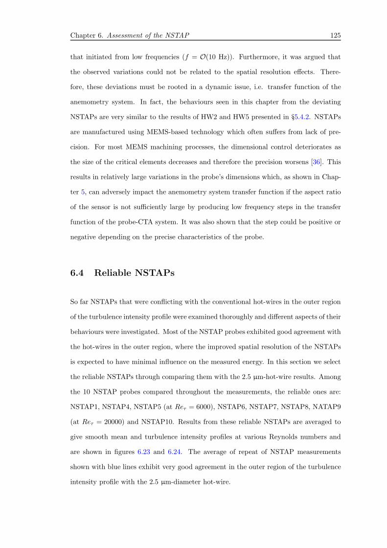
Chapter 6. Assessment of the NSTAP 125
that initiated from low frequencies (f = O(10 Hz)). Furthermore, it was argued that
the observed variations could not be related to the spatial resolution effects. There-
fore, these deviations must be rooted in a dynamic issue, i.e. transfer function of the
anemometry system. In fact, the behaviours seen in this chapter from the deviating
NSTAPs are very similar to the results of HW2 and HW5 presented in §5.4.2. NSTAPsare manufactured using MEMS-based technology which often suffers from lack of pre-
cision. For most MEMS machining processes, the dimensional control deteriorates as
the size of the critical elements decreases and therefore the precision worsens [36]. This
results in relatively large variations in the probe’s dimensions which, as shown in Chap-
ter 5, can adversely impact the anemometry system transfer function if the aspect ratio
of the sensor is not sufficiently large by producing low frequency steps in the transfer
function of the probe-CTA system. It was also shown that the step could be positive or
negative depending on the precise characteristics of the probe.
6.4 Reliable NSTAPs
So far NSTAPs that were conflicting with the conventional hot-wires in the outer region
of the turbulence intensity profile were examined thoroughly and different aspects of their
behaviours were investigated. Most of the NSTAP probes exhibited good agreement with
the hot-wires in the outer region, where the improved spatial resolution of the NSTAPs
is expected to have minimal influence on the measured energy. In this section we select
the reliable NSTAPs through comparing them with the 2.5 µm-hot-wire results. Among
the 10 NSTAP probes compared throughout the measurements, the reliable ones are:
NSTAP1, NSTAP4, NSTAP5 (at Reτ = 6000), NSTAP6, NSTAP7, NSTAP8, NATAP9
(at Reτ = 20000) and NSTAP10. Results from these reliable NSTAPs are averaged to
give smooth mean and turbulence intensity profiles at various Reynolds numbers and
are shown in figures 6.23 and 6.24. The average of repeat of NSTAP measurements
shown with blue lines exhibit very good agreement in the outer region of the turbulence
intensity profile with the 2.5 µm-diameter hot-wire.

Chap
ter6.
Assessm
entoftheNSTAP
126
101 102 103 1045
10
15
20
25
30
U+
(a)
101 102 103 1045
10
15
20
25
30 (b)
101 102 103 1045
10
15
20
25
30
z+
U+
(c)
101 102 103 1045
10
15
20
25
30
z+
(d)
Figure 6.23: Inner normalised streamwise mean velocity U+ against inner normalised wall distance z+ at (a) U∞ = 20 ms−1, x = 6 m, Reτ = 6000,(b) U∞ = 20 ms−1, x = 13 m, Reτ = 10000, (c) U∞ = 20 ms−1, x = 21 m, Reτ = 14500, (d) U∞ = 30 ms−1, x = 21 m, Reτ = 20000. :2.5 µm-diameter hot-wire, : reliable NSTAP measurements, : average of reliable NSTAP measurements. Colour shading is used for the average
of NSTAPs at various Reynolds numbers.

Chap
ter6.
Assessm
entoftheNSTAP
127
101 102 103 1040
2
4
6
8
10
u2+
(a)
101 102 103 1040
2
4
6
8
10(b)
101 102 103 1040
2
4
6
8
10
z+
u2+
(c)
101 102 103 1040
2
4
6
8
10
z+
(d)
Figure 6.24: Inner normalised streamwise broadband turbulence intensity u2+ against inner normalised wall distance z+ at (a) U∞ = 20 ms−1,x = 6 m, Reτ = 6000, (b) U∞ = 20 ms−1, x = 13 m, Reτ = 10000, (c) U∞ = 20 ms−1, x = 21 m, Reτ = 14500, (d) U∞ = 30 ms−1, x = 21 m,Reτ = 20000. : 2.5 µm-diameter hot-wire, : reliable NSTAP measurements, : average of reliable NSTAP measurements. Colour shading is
used for the average of NSTAPs at various Reynolds numbers.

Chapter 6. Assessment of the NSTAP 128
6.5 Summary and conclusions
10 NSTAP probes together with the 2.5 µm-diameter hot-wires were used to measure
streamwise velocity fluctuations in the HRNBLWT facility at various Reynolds numbers.
Of these, NSTAP1, NSTAP2, and NSTAP3 were operated with a modified MUCTA and
the rest (NSTAPs 4-10) were operated with a Dantec Streamline anemometer. Compari-
son of the mean velocity profiles as measured by the NSTAPs and the hot-wire exhibited
very good agreement between all the NSTAPs and the hot-wire. However comparison
of the turbulence intensity profiles revealed some discrepancies between some of the
NSTAPs and the hot-wires in the logarithmic and outer region of the turbulence inten-
sity profiles. Based on the study of Hutchins et al. [47] in this region minimal difference
in resolved energy for wires of different l+ is expected since small-scaled energetic fluc-
tuations (that cannot be fully resolved with the longer hot-wires) are not dominant in
the outer region. Moreover, the observed variations between NSTAPs and the hot-wires
were not consistent, neither in size nor in sign. In fact both magnification and attenua-
tion of turbulence intensity were observed for different NSTAP probes when compared
to the hot-wires. An investigation of the premultiplied energy spectra revealed that
the energy deviation in those NSTAPs, which disagreed with the hot-wires in the outer
region of the turbulence intensity profiles, initiated at very low frequencies (∼ 10 Hz).
Measurements with both the MUCTA and the Dantec Streamline contained reliable
NSTAPs and unreliable NSTAPs. This rules out the effect of the anemometer in the
conflicting behaviours of some NSTAPs. Reliable NSTAPs refers to the NSTAP probes
that agree with the 2.5 µm-diameter hot-wire in the outer region of the turbulence
intensity profiles, with the remaining NSTAP probes referred to as unreliable.
The effect of pitch angle was investigated on the NSTAPs by conducting measurements
with two probe holder angles θ = 3 and 10. These measurements revealed attenuation
in the turbulence intensity in the near wall region for θ = 10. No differences were
observed in the outer region of the intensity profiles by changing θ, eliminating a role

Chapter 6. Assessment of the NSTAP 129
of the probe holder angle in the discrepancies between different NSTAPs and hot-wires
observed here.
The effect of the ambient temperature variations during the measurements and quality
of the calibration curves were discussed as well. It was shown in Appendix A that
the ambient temperature variations have minimal effects on the results of the NSTAPs.
Also, comparing calibration curves of three NSTAP probes revealed no differences that
could explain the observed discrepancies in their measured energy. All the NSTAPs that
we started the measurements with had similar physical characteristics, namely similar
appearances and electrical resistances. The reason for the anomalous behaviour of some
of the NSTAPs remains an open topic for further studies.

Chapter 7
Well-resolved measurements in
turbulent boundary layer flows
Nano-Scale Thermal Anemometry Probes (NSTAP) [6] together with conventional hot-
wire probes are used to measure streamwise velocity fluctuations in turbulent boundary
layer flow at Reτ = 6000, 10000, 14500, 20000 and 25000. A summary of the mea-
surement conditions are shown in table 7.1. Multiple measurement repeats were carried
out at each Reynolds number (number of these repeats is given by N in table 7.1) and
reliable NSTAPs have been selected through analysis detailed in chapter 6. These N
repeats are averaged to obtain the averaged NSTAP at each Reτ . In this chapter results
from the reliable NSTAPs are reported in six sections: § 7.1 Streamwise mean velocity § 7.2 Streamwise turbulence intensity § 7.3 Spectra of the streamwise velocity fluctuations § 7.4 Spectrograms § 7.5 Skewness and kurtosis § 7.6 Turbulence energy dissipation rate and Kolmogrov scale characteristics
130

Chap
ter7.
Well-reso
lvedmeasurem
ents
inturbu
lentboundary
layer
flows
131
Table 7.1: Summary of the experimental conditions presented in this chapter.
Reτ x U∞ ν/uτ uτ δ TU∞/δ ∆t+ l+ Probes N Symbols/(m) (ms−1) (µm) (ms−1) (m) lines
6000 6.3 20 23.6 0.69 0.142 14400 0.58 21 HW -2.54 averaged NSTAP 6
10000 13 20 24.4 0.66 0.245 12500 0.54 20.5 HW -2.46 averaged NSTAP 4
14500 21 20 25.2 0.65 0.366 14000 0.51 19.8 HW -2.38 averaged NSTAP 3
20000 21 30 17.2 0.93 0.345 12500 0.68 29.0 HW -3.48 averaged NSTAP 5
25000 21 40 13.9 1.22 0.34 16500 1.1 36.0 HW -

Chapter 7. Well-resolved measurements in turbulent boundary layer flows 132
7.1 Streamwise mean velocity
The streamwise mean velocity profile has been extensively studied in turbulent boundary
layer flows (e.g. Osterlund [106]), channel flows (e.g. Monty [94]), and pipe flows (e.g.
Zagarola and Smits [159]). The studies support the existence of a logarithmic relation
in the overlap region known as the law of the wall
U
uτ=
1
κlog(
zuτν
) +A (7.1)
where κ and A are universal constants in smooth wall turbulent flows. The universality
of these constants have been questioned recently, with a wide range of κ reported for
different types of wall-bounded turbulent flows (0.37-0.436 [78]). However, using experi-
mental data in the Reynolds number range 2×10⁴ < Reτ < 6×10⁵ for boundary layers,
pipe flow and the atmospheric surface layer, Marusic et al. [79] showed within experi-
mental uncertainty, the data support the existence of a universal logarithmic region.
Figure 7.1(a) and (b) show the mean velocity profiles as measured by the NSTAP probes
and conventional 2.5µm-diameter hot-wires together with the DNS data from Sillero
et al. [128] in inner normalised and velocity defect form, respectively. Note that there
is excellent agreement between the NSTAP and the hot-wire where both are available.
It should also be noted that the boundary layer thickness has been calculated by fitting
the composite profile of Chauhan et al. [18]. Sillero et al. [128] used δ99 to determine
the boundary layer thickness yielding Reτ = δ+99 ≈ 1990, while if the composite profile
fit is used to estimate the boundary layer thickness Reτ = δ+com ≈ 2500 is obtained.
It is evident that all the profiles, when shown in the inner normalised form, follow the
equation 7.1 with κ = 0.384 and A = 4.17 in the overlap region. The profiles in the
velocity defect form in the overlap region follow
U∞ − U
uτ= B − 1
κlog(
z
δ) (7.2)

Chapter 7. Well-resolved measurements in turbulent boundary layer flows 133
with B = 2.3.
101 102 103 1040
5
10
15
20
25
30
z+
U+
(a)
10-3 10-2 10-1 1000
5
10
15
20
25
30
z/δ
U+ ∞−
U+
(b)
Figure 7.1: (a) Inner normalised mean velocity U+ against inner normalised walldistance z+. Straight dot-dashed line indicates the log-law U+ = 1/0.384 ln(z+)+4.17.(b) Velocity defect law against outer normalised wall distance z/δ. Straight dot-dashedline corresponds to the relation U+ = 2.3− 1/0.384 ln(z/δ). : NSTAP-Reτ = 6000,
: NSTAP-Reτ = 10000, : NSTAP-Reτ = 14500, : NSTAP-Reτ = 20000, :hot-wire at the Reτ in which NSTAP is used, : hot-wire data at Reτ = 25000, :
DNS at δ+99 = 1990 (Sillero et al. [128]).

Chapter 7. Well-resolved measurements in turbulent boundary layer flows 134
7.2 Streamwise turbulence intensity
While the mean flow field has received the majority of attention over the past few
decades, the streamwise turbulence intensity (u2) has also been the subject of a consid-
erable number of studies [78].
A profile of the streamwise turbulence intensity scaled on uτ (u2+) can be divided into
four main regions within the boundary layer. The region closest to the wall (0 ≤ z+ ≤
100) is referred to as the near-wall region, which is followed by the intermediate region in
the range 100 ≤ z+ ≤ 3.9Re1/2τ . The inertial sublayer (or logarithmic region) is located
in the range 3.9Re1/2τ ≤ z+ ≤ 0.15Re. Finally we have the outer region in the range
0.15Re ≤ z+ ≤ Reτ . These regions will be discussed in detail in the following sections.
7.2.1 The near-wall region in the streamwise turbulence intensity
In the near-wall region a maximum appears in the streamwise turbulence intensity pro-
file, known as the inner peak. The inner normalised wall normal location of this peak
is commonly accepted to be independent of the Reynolds number and fixed at z+ ≈ 15.
However, the Reynolds number scaling of the magnitude of the inner peak has been
controversial. While most of the recent studies show that the inner peak exhibits a weak
Re dependence (De Graaff and Eaton [25], Hutchins and Marusic [46], Klewicki and
Falco [59], Lee and Moser [67], Metzger et al. [86], among others), Superpipe and HRTF
data (Hultmark et al. [44, 45], Vallikivi et al. [147]) show that this peak is invariant with
Re. It is however pointed out that experimental uncertainty could be masking any weak
Re dependence. The studies that support the growth of the inner peak with Re took
special care to ensure that spatial resolution issues did not influence the results, since
several studies suggest that finite probe size leads to the attenuation of the turbulence
intensity in the near-wall region (Johansson and Alfredsson [53], Willmarth and Sharma
[154], Ligrani and Bradshaw [72], Hites [40], and Hutchins et al. [47]).

Chapter 7. Well-resolved measurements in turbulent boundary layer flows 135
Figure 7.2(a) and (b) show the turbulence intensity profiles scaled with uτ at various
Reτ against inner and outer normalised wall distance respectively. The NSTAP and
the conventional hot-wire exhibit very good agreement in the outer region where spatial
resolution influence is minimal. While the hot-wire results do not show a clear Reτ
trend for the inner peak (because of spatial resolution effects), NSTAP measurements
exhibit a growth of the inner peak with increasing Reτ . As l+ < 3.5 for all the NSTAP
measurements, we can compare our results with the DNS from Sillero et al. [128] to see
the low Reynolds number effect on the inner peak trend. The inner peak values scaled
on uτ are plotted against Reτ in figure 7.3 for the data from the current study as well
as for DNS of boundary layer [128] and channel flow [41]. Also inner peaks measured
in the Superpipe and HRTF are shown at the Reynolds numbers where the peak has
been resolved. It is evident that our experimental results extends the logarithmic trend
of u2+max previously seen in the DNS data. Dependence of the peak in u2+on Reτ was
fitted to the boundary layer DNS and our higher Re boundary layer data to obtain
u2+max = 3.54 + 0.646 log(Reτ ). (7.3)
This relation is shown in figure 7.3 together with the correlations proposed by Lee
and Moser [67] (u2+max = 3.66 + 0.646 log(Reτ )) and Monkewitz and Nagib [91] (their
equation 4.1). While proximity of the two former equations is evident, one can see that
the latter underpredicts u2+max for Reτ < 1000 and overpredicts it for Reτ > 1000 (at
least in the domain shown here).
Another way of understanding the near wall behaviour of the turbulence intensity
is decomposing u2+ into small-scale u2s+ and large-scale u2l
+components such that
u2+ = u2s+ + u2l
+[77]. In order to compute these components, the fluctuating u+
signal was separated into small-scale u+s (λx < 10000) and large-scale u+l (λx > 10000)
components using a sharp cut-off spectral filter. Then small-scale and large-scale
variances (u2s+ and u2l
+) were computed separately from these high and low pass filtered
components. The choice of the cut-off wavelength was based on the information found

Chapter 7. Well-resolved measurements in turbulent boundary layer flows 136
in the energy spectra presented in §7.3.1. It will be shown that energy spectra in the
near wall region collapse in the domain λx < 10000 for the Reτ range of this study. The
results of this decomposition are shown in figure 7.4. It can be seen that the small-scale
101 102 103 1040
2
4
6
8
10
z+
u2+
(a)
10-3 10-2 10-1 1000
2
4
6
8
10
z/δ
u2+
(b)
Figure 7.2: Inner normalised turbulence intensity profile u2+ against (a) innernormalised wall distance z+; (b) outer normalised wall distance z/δ. Dotted line
corresponds to u2+max = 5.4 − 0.642 log(zmax/δ). Dot-dashed line corresponds to
u2+ = 1.95 − 1.26 log(z/δ). : NSTAP-Reτ = 6000, : NSTAP-Reτ = 10000, :NSTAP-Reτ = 14500, : NSTAP-Reτ = 20000, : hot-wire at the Reτ in which
NSTAP is used (grey color is used for z+ < Re1/2τ for clarity), : hot-wire data at
Reτ = 25000, : DNS at δ+99 = 1990 (Sillero et al. [128]).

Chapter 7. Well-resolved measurements in turbulent boundary layer flows 137
components are invariant with Reτ while the large-scale components increase with
Reτ leading to the increasing trend of the u2+ in the near-wall region. Large-scale
components exhibit a peak shown with diamonds in figure 7.4. Mathis et al. [82] used
the Reynolds number trend of these peaks compared to the trend of the large-scale
components at the location of the inner peak (z+ ≈ 15) to argue that the outer peak
of the total intensity surpasses the inner peak of the total intensity at extremely high
Reynolds numbers. This approach might result in a misleading conclusion, since while
the small-scale component is invariant with Reτ at the location of the inner peak, it
decreases with the Reτ at the location of the outer peak. Moreover, the location and
the intensity of the outer peak is subject to experimental errors around the outer peak.
In §7.2.3 a new method to find an upper limit for the outer peak will be proposed.
102 103 104 105
7
7.5
8
8.5
9
9.5
10
10.5
11
Reτ
u2+max
Figure 7.3: Dependence of maximum of u2+ on Reτ . : averaged NSTAP,: NSTAP measurement repeats, : Superpipe data [45], : HRTF data [147], :
boundary layer DNS [128], : channel DNS [41], : u2+max = 3.54+0.646 log(Reτ ),
: u2+max = 3.66 + 0.642 log(Reτ ) from Lee and Moser [67], : equation (4.1) in
Monkewitz and Nagib [91].

Chapter 7. Well-resolved measurements in turbulent boundary layer flows 138
101 102 103 1040
1
2
3
4
5
6
7
8
9
z+
u2+
Figure 7.4: Streamwise turbulence intensity profiles decomposed into small-scale(λ+
x < 10000, solid lines) and large-scale (λ+x > 10000, dashed lines) components for
the NSTAP measurements shown in figure 7.2. Solid diamonds show the location ofthe peak in the large-scale component of the turbulence intensity.
7.2.2 The inertial sublayer and the outer region in the streamwise
turbulence intensity
Recent turbulence experiments provide convincing evidence that at sufficiently high
Reτ , streamwise turbulence intensity follows a logarithmic decay before the onset of
the wake region (see e.g. Hultmark et al. [44, 45], Marusic et al. [79, 80], Orlu et al.
[105]). Townsend [140] proposed that the scaling from the wall can be associated with
corresponding attached eddies. The geometric lengths of these eddies scale with z, and
have population densities per characteristic eddy height that scale inversely with z.
Townsend showed that this argument leads to a logarithmic profile for the streamwise
(and spanwise) turbulence intensities of the form
u2+ = B1 −A1 log(z/δ), (7.4)

Chapter 7. Well-resolved measurements in turbulent boundary layer flows 139
where δ is the boundary layer thickness (or pipe radius or channel half-height). It can be
seen in figure 7.2(b) that our experimental results follow this equation reasonably well
with A1 = 1.26 and B1 = 1.95 as previously given by Marusic et al. [79] by analysing
high Reτ data obtained in different facilities. The upper bound of the logarithmic region
appears to be z/δ = 0.15. With increasing Reτ , the region for which equation 7.4 is valid,
expands towards the wall. That is, the lower bound of this logarithmic region in viscous
scaling is believed to be proportional to Re1/2τ (z+ ∝ Re
1/2τ ) so that z/δ ∝ Re
−1/2τ . For
the DNS data at Reτ ≈ 2500 no clear logarithmic region is observed although its u2+
profile against z/δ follows the profiles corresponding to higher Reynolds numbers in the
outer region (z/δ > 0.15). The lack of logarithmic region for the DNS data can be
attributed to the insufficient scale separation as the Reτ is relatively low.
The scaling of the turbulence intensity profile in the outer region has received less at-
tention. For this region, McKeon and Morrison [83] report that u2+ profiles as functions
of z/δ collapse in pipe flow, but in different manners for high and low Reynolds num-
bers. They associate this behaviour to the relatively slow development of self-similarity
of the spectrum. Marusic et al. [80] report a very good collapse of u2+ profiles in the
outer scaling for the Reynolds number range 2800 ≤ Reτ ≤ 13400 in the turbulent
boundary layer flow. The results of the current study also show very good collapse of
the intensity profiles in outer region with outer scaling for the Reynolds number range
2500 ≤ Reτ ≤ 25000 as seen in figure 7.2.
7.2.3 The intermediate region in the streamwise turbulence intensity
Thanks to the uniquely high Reynolds number data of the Superpipe, many new aspects
of turbulence have been revealed, one of which is the possibility of the emergence of a
second outer peak in the streamwise turbulence intensity profile, of which both the
location and intensity may depend on Reτ . The outer peak has been reported for Reτ ≥
20000 (Hultmark et al. [44] and Hultmark et al. [45]). However, the presence of this
peak and as to whether it is a peak or a plateau is not still clear since spatial resolution
of the Superpipe measurements degrades for the very high Reτ measurements where the

Chapter 7. Well-resolved measurements in turbulent boundary layer flows 140
outer peak is noticeable. According to Hutchins et al. [47] the spatial resolution filtering
extends to wall distances higher than the immediate near-wall region and may produce
a delusive outer peak. The prediction of a second outer peak arising at high Reynolds
number would be notable as it may indicate the presence of new outer phenomena
[44, 78].
We address this problem in this section since spatial filtering is not an issue in our
measurements up to Reτ = 20000 (obtained with the NSTAP). Our Reynolds numbers
are not as high as those in the studies of Hultmark et al. [44, 45], however, our highest
well-resolved Reτ case is equal to the lowest Reτ case in their study where the outer
peak was reported. In fact, our results exhibit the presence of plateaus for Reτ = 14500
and 20000, and it can be seen that locating the outer peak accurately is challenging
due to the lack of smoothness of the intensity profiles. This issue can be remedied by
trying to find an upper bound for the outer peak instead of the peak itself. To this
end, a logarithmic line, tangent to the intermediate part of the intensity profile at the
inflection point of the profile is drawn as shown in figure 7.5. The inflection point in
the intermediate region is associated with the point where d2(u2+)/d(log z+)2 changes
sign; and the tangent line is fitted to totally four to five points in the profile around the
inflection point. The intersection of this tangent line with the logarithmic equation 7.4
gives the upper bound for the outer peak. The tangent lines show emergence of an outer
peak which becomes more evident with increasing the Reτ . Figure 7.6(a) and (b) show
the Reτ dependency of the intensity (shown by u2p+int
) and location (shown by (z/δ)pint)
of the intersections respectively. Dependency of the slope of the tangent logarithmic line
Sint is shown in figure 7.6(c). These points can be fitted using appropriate functions to
obtain
u2p+int
= −2.99 + 0.98 log(Reτ ), (7.5a)
(z/δ)pint = 32.66Re−0.73τ , (7.5b)
Sint = −2.42 + 0.25 log(Reτ ). (7.5c)

Chapter 7. Well-resolved measurements in turbulent boundary layer flows 141
10-3 10-2 10-1 1000
2
4
6
8
10
z/δ
u2+
Figure 7.5: Reynolds number dependency of the logarithmic tangent line to theintermediate region in the turbulence intensity profile of the NSTAP measurementsshown in figure 7.2. The inset shows the zoomed view of the region bounded by the
rectangle demonstrating the slope (Sint) and x ((z/δ)pint) and y (u2p+
int) coordinates
of the intersection of the tangent line (to the intermediate region) with the logarithmicrelation for Reτ = 6000.
Marusic et al. [79] used z/δ = 3Reτ−1/2 as the lower bound of the logarithmic region and
Mathis et al. [82] used z/δ = 3.9Reτ−1/2 as the location of the outer peak. Therefore,
an exponential function is used here to find the correlation for the Reynolds number
trend of (z/δ)pint since it is analogues to the outer peak location. Also shown in figure
7.6(a) and (b) (by diamonds) are the total intensity (total of large-scale and small-scale
intensity) and z/δ location of the large-scale component peak as shown in figure 7.4,
together with the curve fits used by Mathis et al. [82] (u2p+ = −2.13+0.84 log(Reτ ) and
z/δ = 3.9Reτ−1/2). Very good agreement is seen between our correlation for the wall
normal-location of the intersection ((z/δ)pint = 32.66Re−0.73τ ) and z/δ = 3.9Reτ
−1/2 for
high Reτ . While, as expected, our curve fit for the intensity of the intersection u2p+int
over predicts the outer peak magnitude since it is introduced as an upper bound.

Chapter 7. Well-resolved measurements in turbulent boundary layer flows 142
103 104 1050
2
4
6
8
10
-3.06+0.99log(Reτ)
-2.13+0.84log(Reτ)
103 104 1050
0.05
0.1
0.15
0.2
0.25
32.661/Reτ
0.73
3.9/Reτ
0.5
103 104 105-1
-0.5
0
0.5
-2.42+0.25log(Reτ)
Reτ
ReτReτ
u2 p+in
t
(z/δ) p
int
Sin
t
(a) (b)
(c)
Figure 7.6: Reynolds number dependency of (a) the y-coordinate of the intersectionof the tangent line to the turbulence intensity profile at its inflection point with the
logarithmic equation 7.4 given by u2p+
int( ) and the total inner normalised turbulence
intensity at the location of peak in the large-scale component of the turbulence intensity( ); (b) the x-coordinate of the intersection points given by zint/δ ( ) and theouter normalised wall-normal location of the peak in the large-scale component of theturbulence intensity ( ); (c) slope of the tangent lines in the intermediate region,Sint. : curve fits to the intersection values versus Reτ in (a) and (b) and slopeof the logarithmic curve tangents as a function of Reτ in (c). : curve fits proposedby Mathis et al. [82] for the Reynolds number dependency of the total turbulenceintensity at the peak of the large-scale component of the turbulence intensity in (a) andReynolds number dependency of the wall-normal location of the peak in the large-scale
component of the turbulence intensity in (b).
Having these correlations one can determine the logarithmic tangent line to the inter-
mediate region for any Reτ ≥ 6000 using
u2+ = u2p+int
+ Sint log
[
z/δ
(z/δp)int
]
. (7.6)
Equations 7.5 and 7.6 are used to predict the intermediate region in the turbulence
intensity profile for Reτ = 40000 and 1× 10⁶. This region together with the logarithmic

Chapter 7. Well-resolved measurements in turbulent boundary layer flows 143
101 102 103 104 105 1060
2
4
6
8
10
12
SLTEST-[Metzger et al, 2007]-HWSLTEST-[Metzger et al, 2007]-SonicSLTEST-[Hutchins et al, 2012]-SonicCICLoPE-[Willert et al, 2017]-PIV
z+
u2+
Figure 7.7: Comparison of u2+ for the SLTEST surface layer and CICLoPE pipeexperiments with the logarithmic model of equation 7.4 ( ) and intermediate regioncorrelation of equation 7.6 ( ). : SLTEST hot-wire data of Metzger et al. [84],
: SLTEST sonic data of Metzger et al. [84], : SLTEST sonic data of Hutchinset al. [48], : CICLoPE pipe PIV data of Willert et al. [153] at Reτ = 40000. Thefriction Reynolds numbers for the data from Metzger et al. [84] and Hutchins et al. [48],
are estimated as Reτ ≈ 7.7× 10⁵ and Reτ ≈ 7.8× 10⁵, respectively.
region for these Reynolds numbers are shown in figure 7.7 where they are compared with
the SLTEST data from Metzger et al. [84] and Hutchins et al. [48] (at Reτ ∼ O(106)) and
CICLoPE data from Willert et al. [153] (at Reτ = 40000). The agreement between the
model predictions and the SLTEST data, especially in the intermediate region, is very
good; and acceptable agreement is seen between the model prediction and the CICLoPE
data.
Equations 7.3 and 7.5a can be used to predict whether at sufficiently high Reτ the outer
peak overcomes the inner peak. The extrapolated result in figure 7.8 shows that such
behaviour happens around Reτ = 108. Note that since we are using an upper bound for
the outer peak (equation 7.5a), this is a lower bound for the predicted Reτ . In fact, if we
use the correlation proposed by Mathis et al. [82] for Reτ dependence of the outer peak
intensity (0.84 log(Reτ ) − 2.13), the predicted Reτ at which the outer peak overcomes
the inner peak exceeds 1012. Also, one should acknowledge that these predictions are
valid if the inner and the outer peak trends remain unchanged up to these extreme

Chapter 7. Well-resolved measurements in turbulent boundary layer flows 144
103 104 105 106 107 108 109 10102
4
6
8
10
12
14
16
18
Reτ
u2+
Figure 7.8: Comparison of the Reynolds number dependency of the inner peak givenby equation 7.3 ( ) and the outer peak ( ) used by Mathis et al. [82] as well as they-coordinate of the intersection of the log-region curve fit and the tangent line to thetransition region given by equation 7.5a ( ). Symbols are as in figures 7.3 and 7.6.
values for Reτ . Such questions remain controversial [44, 77, 84, 96] since accurate near-
wall measurements up to high Reτ face significant challenges. This makes any prospect
of this phenomenon tentative. However, according to our data and the atmospheric
surface layer data [85] it is unlikely that this phenomenon happens at laboratory scale
or terrestrial Reτ (if it ever happens).
7.2.4 Spatial resolution filtering in near-wall region
Several correction schemes for spatial filtering of single component hot-wire measure-
ments have been proposed recently (Chin et al. [20], Monkewitz et al. [90], Philip et al.
[117], Segalini et al. [127], Smits et al. [131]). Comparison of all these corrections is
out of the scope of this thesis. For a full assessment and comparison of these methods
refer to Miller et al. [87]. The abundance of this type of study in literature highlights
the importance of accurate near-wall data in wall-bounded turbulent flows up to high
Reynolds number, which is scarce. Therefore, spatial correction schemes are usually used
to deduce the correct turbulence intensity from spatially filtered hot-wire data at high
Reτ . In this section we employ our well-resolved data to assess the correction scheme

Chapter 7. Well-resolved measurements in turbulent boundary layer flows 145
of Smits et al. [131] which is the most highly cited, and also the scheme used to correct
the NSTAP data in the Superpipe and the HRTF.
Figure 7.9 shows u2+ as measured with the NSTAP and the 2.5 µm-diameter hot-wire
together with the Smits et al. [131] corrcted hot-wire profiles for various Reτ . It is noted
101 102 103 1040
2
4
6
8
10 Reτ = 6000
l+HW = 21
u2+
(a)
101 102 103 1040
2
4
6
8
10 Reτ = 10000
l+HW = 20.5
(b)
101 102 103 1040
2
4
6
8
10 Reτ = 14500
l+HW = 20
z+
u2+
(c)
101 102 103 1040
2
4
6
8
10 Reτ = 20000
l+HW = 29
z+
(d)
101 102 103 1040
2
4
6
8
10 Reτ = 25000
l+HW = 36
z+
u2+
(e)
Figure 7.9: Streamwise turbulence intensity measured with the hot-wires and theNSTAP probes at various Reτ where : uncorrected hot-wires’ data, : correctedhot-wires’ data for spatial resolution using the scheme proposed by Smits et al. [131],
: NSTAP-Reτ = 6000 , : NSTAP-Reτ = 10000 , : NSTAP-Reτ = 14500 and: NSTAP-Reτ = 20000.(a) Reτ = 6000, (b) Reτ = 10000, (c) Reτ = 14500, (d)
Reτ = 20000.

Chapter 7. Well-resolved measurements in turbulent boundary layer flows 146
that the NSTAP results are not corrected for spatial resolution since their associated l+
is small enough to ensure that all the small-scale turbulence energy content is resolved. It
can be seen that the correction works reasonably well for measurements at Reτ = 6000,
10000, and 14500 where inner normalised hot-wire length l+HW ≈ 20. However, for
Reτ = 20000 with l+HW = 29, its performance degrades resulting in an underestimation
of the turbulence intensity around the inner peak (z+ = 15). This may indicate that
performance of this correction scheme for Reτ out of the range that it has been validated
in the original paper (Reτ ≥ 10000) might not be as accurate as previously thought.
7.3 Spectra of the streamwise velocity fluctuations
A wide range of eddy sizes are present in the turbulent motions. Quantifying the con-
tribution of various scales to the turbulent kinetic energy improves our understanding
of turbulence. This can be done through use of Fourier decomposition. In this method
the turbulence signal is decomposed into a spectrum of wave-numbers to find the one
sided spectral power density φij at each wave number. Unfortunately, experimentally
measuring the full three dimensional energy spectrum is extremely difficult, as one needs
fully resolved three dimensional velocity data. Instead, we can often only examine the
power spectral density of the streamwise velocity fluctuations φuu as a function of the
streamwise wave-numbers kx. In order to deduce spatial spectra from the time series
data obtained from the stationary hot-wire, Taylor’s frozen turbulence hypothesis (Tay-
lor [138]) is employed. It can be shown that the integral of φuu over kx is equal to the
streamwise turbulent stress
∫ ∞
0φuudkx = u2. (7.7)
In this section energy spectra of the well-resolved measurements in the turbulent bound-
ary layer flow are examined in two different subsections: (i) the near-wall region , (ii)
the inertial sublayer.

Chapter 7. Well-resolved measurements in turbulent boundary layer flows 147
7.3.1 Energy spectra in the near-wall region
We start this section with a dimensional analysis for the streamwise energy spectrum
φuu. The spectrum can be separated into three wave-number domains :
1. Small wave-number motions: In this domain, although near the wall, the boundary
layer thickness is important since the contributing large-scale motions are of the
order of the boundary layer thickness, δ. Hence, the relevant variables are φuu,
kx, friction velocity uτ , kinematic viscosity ν, wall-distance z, and boundary layer
thickness δ. A dimensional analysis leads to
kxφuu
u2τ= f1(kxz, z
+, z/δ) = f1(k+x z
+, z+, z+/δ+). (7.8)
Here ‘+’ indicates inner normalisation, i.e. normalisation using friction velocity
uτ and kinematic viscosity ν. Equation 7.8 implies that in the near wall region
over the small wave-number domain, kxφuu/u2τ is dependant on Reτ as well as k+x
and z+.
2. Moderate to high wave-number motions: In this wave-number domain in the near-
wall region, the relevant variables are φuu, kx, uτ , z, and ν. Here, since z/δ ≪ 1
for sufficiently high Reτ , δ is not important. Therefore, a dimensional analysis
yields
kxφuu
u2τ= f2(kxz, z
+) = f2(k+x z
+, z+). (7.9)
Therefore, in this domain kxφuu/u2τ can be expressed in terms of k+ and z+ only.
3. Very high wave-number motions: In this range of motions, φuu is dependent on
wave-number kx, Kolmogrov’s length scale η and Kolmogrov’s velocity scale vη.
Here, vη = (νǫ)1/4 and η = (ν3/ǫ)1/4 where ν is kinematic viscosity and ǫ is the
dissipation rate. With these variables two non-dimensional parameters can be
considered such that

Chapter 7. Well-resolved measurements in turbulent boundary layer flows 148
kxφuu
v2η= f3(kxη) = f3(k
+x η
+). (7.10)
It will be shown in §7.6 that in the near-wall region and the inertial sublayer,
η+ and v+η can be expressed as functions of innernormalised wall-distance z+,
independent of Reτ , i.e. η+ = hη(z+) and v+η = hv(z
+). Therefore, equation 7.10
can be rewritten as
kxφuu
u2τ= [hv(z
+)]2f3(k+x hη(z
+)) (7.11)
which shows that in this wave-number domain, similar to moderate to high wave-
number motions, kxφuu/u2τ is a function of k+ and z+ and independent of Reτ .
The above arguments indicate that at a fixed z+ in the near-wall (sufficiently small z/δ),
kxφuu(k+)/u2τ (or equivalently kxφuu(λ
+x )/u
2τ where λx = 2π/kx is the wave-length)
curves should collapse over medium to very high wave-numbers (medium to very low
wave-lengths) when various Reτ are compared, and an Reτ dependency is expected
in the low wave-number (high wave-length) end of the spectra only. Since small-scale
energy can be significantly affected by spatial resolution (as documented by Hutchins
et al. [47] and Chin et al. [19]), the data here may be helpful to clarify the small-scale
behaviour in the near-wall. The inner-scaled, pre-multiplied energy spectra kxφuu/u2τ
is plotted against streamwise wavelength, λ+x , in figure 7.10 at the peak turbulence
intensity location, z+ ≈ 15 for the experimental data (Reτ = 6000, 10000, 14500, and
20000) as well as channel DNS data of Hoyas and Jimenez [41] (Reτ = 550, 2000)
and boundary layer DNS data of Sillero et al. [128] (δ+99 = 1990). Here, spectra are
plotted in premultiplied form so that equal areas equate to equal contributions to the
turbulence intensities on the semilogorithmic plot:∫∞0 φuudkx =
∫∞0 kxφuud(log kx) =
∫∞0 kxφuud(log λx) = u2.
All the spectra appear to collapse well for the wave-lengths below λ+x ≈ 1500 and the
experimental spectra (Reτ ≥ 6000) collapse well for the wave-lengths below λ+x ≈ 15000.

Chapter 7. Well-resolved measurements in turbulent boundary layer flows 149
101 102 103 104 105 106 1070
0.5
1
1.5
2
2.5
λ+x
kxφuu/u
2 τ
Figure 7.10: Comparison of premultiplied energy spectra at z+ ≈ 15 from variousReynolds numbers and flow geometries. : NSTAP-Reτ = 6000 , : NSTAP-Reτ = 10000 , : NSTAP-Reτ = 14500, : NSTAP-Reτ = 20000, : DNSboundary layer-δ+99 = 1990 [128], : DNS channel-Reτ ≈ 2000 , : DNS channel-
Reτ ≈ 550 [41]. The arrow indicates increase in the Reτ for the NSTAP spectra.
Moreover, in the high wave-length end of the spectra an increasing trend with Reτ is
evident. These observations are consistent with the experimental study of Hutchins
et al. [47] in the boundary layer flow (up to Reτ ≈ 19000) where hot-wire sensors with
lengths of 22 wall units were used, and for the lower Reynolds number DNS studies of
Hoyas and Jimenez [41] (up to Reτ ≈ 2000) in the channel flow, and Chin et al. [21]
(up to Reτ ≈ 2000) in the pipe flow. The peak of the innernormalised premultiplied
energy spectra is seen to remain constant at kxφuu/u2τ ≈ 2.2 at the innernormalised
wave-length λ+x ≈ 850. It should also be noted that the small-scale energy is not only
invariant with Reτ , but independent of the flow geometry since channel and boundary
layer flow spectra in the small-scale region appear to collapse well. Figure 7.11 shows the
same plots for the experimental data at other innernormalised wall-distance locations.
It can be seen that the kxφuu/u2τ curves collapse for wave-lengths below λ+
x ≈ 15000 up
to z+ = 280 for the Reynolds number range 6000 ≤ Reτ ≤ 20000. Only at z+ = 670
the Reτ = 6000 spectrum starts to deviate from the spectra of other Reynolds numbers
in the small-scale region. This behaviour in the spectra explains the increasing trend
with Reτ for the peak u2+ in the near-wall region (There is an increasing amount of

Chapter 7. Well-resolved measurements in turbulent boundary layer flows 150
101 102 103 104 105 106 1070
0.2
0.4
0.6
0.8
1
1.2
1.4
1.6
1.8z+ =24
kxφuu/u
2 τ
(a)
101 102 103 104 105 106 1070
0.2
0.4
0.6
0.8
1
1.2z+ =47(b)
101 102 103 104 105 106 1070
0.2
0.4
0.6
0.8
1z+ =92
kxφuu/u
2 τ
(c)
101 102 103 104 105 106 1070
0.2
0.4
0.6
0.8
1
1.2 z+ =178(d)
101 102 103 104 105 106 1070
0.2
0.4
0.6
0.8
1
1.2 z+ =277
λ+x
kxφuu/u
2 τ
(e)
101 102 103 104 105 106 1070
0.2
0.4
0.6
0.8
1
1.2
1.4z+ =670
λ+x
(f)
Figure 7.11: Reynolds number dependence of premultiplied energy spectra as mea-sured with the NSTAP at (a) z+ ≈ 25, (b) z+ ≈ 50 , (c) z+ ≈ 90, (d) z+ ≈ 180, (e)z+ ≈ 280, (f) z+ ≈ 670. : Reτ = 6000 , : Reτ = 10000, : Reτ = 14500 and
: Reτ = 20000.
large-scale superimposed energy in the near-wall region as Reτ increases). This scaling
law in the near-wall region is in close accordance with the “spectral analogue of the law
of the wall” by Zamalloa et al. [160].
7.3.2 Energy spectra in the inertial sublayer and the outer region
Let’s consider the distribution of the u-power spectra φuu in the wall-distance region
where the energy-containing motions are independent of viscosity, i.e. ν/uτ ≪ z. The
relevant variables to express φuu in the range of energy-containing motions are kx, uτ , z,

Chapter 7. Well-resolved measurements in turbulent boundary layer flows 151
and δ. According to the Buckingham’s Π-theorem, three dimensionless parameters are
sufficient to express the solution, however, five dimensionless parameters are possible
: φuu/δuτ2, φuu/zuτ
2, kxδ, kxz, z/δ. We separate the viscous-independent energy-
containing spectral region into two separate regions to take into account all the above
dimensionless parameter.
1. Small wave-number motions (kx ∼ 1/δ): At these wave-numbers kx scales as 1/δ.
Therefore, we can normalise kx with δ and expect a δ-scaling law of the form
φuu(kxδ, z/δ)
u2τ= g1(kxδ, z/δ) =
φuu(kx, z/δ)
δu2τ. (7.12)
Here φuu(kxδ, z/δ) is the power-spectral density per unit non-dimensional wave-
number kxδ at outer-normalised wall-distance z/δ. This scaling is demonstrated
in figure 7.12 for the experimental results for various Reynolds numbers in the
logarithmic region (3Re0.5τ ≤ z+ ≤ 0.15Reτ ). We can see that plotting the energy
spectra against kxδ does not collapse the spectra around the small wavenumber
peaks/plateaus. This shows the dependence of the spectra on z/δ as well as kxδ
suggesting that even in the logarithmic region z cannot be ignored as a relevant
variable in this range of motions. However, it appears that for the higher Reτ
cases (figures 7.12(d),(e)) where logarithmic region extends to relatively small z/δ
values towards the wall (z/δ ∼ 2 × 10⁻²) we start to see that the dependence on
z/δ vanishes for a small wall-distance region located at the start of the logarith-
mic region where the magnitudes of the peaks/plateaus remain almost constant
with decreasing z/δ. In this region ν/uτ ≪ z ≪ δ is valid and equation 7.12
approximately reduces to
φuu(kxδ)
u2τ= g1(kxδ) =
φuu(kx)
δu2τ, (7.13)
as shown by Perry et al. [115] in the context of Townsend’s attached eddy hy-
pothesis [140]. It is expected that with increasing Reτ this z/δ-independent region
extends towards the wall.

Chapter 7. Well-resolved measurements in turbulent boundary layer flows 152
10-2 10-1 100 101 102 103 1040
0.2
0.4
0.6
0.8
1
1.2
1.4Reτ = 6000
kxφuu/u
2 τ
(a)
10-2 10-1 100 101 102 103 1040
0.2
0.4
0.6
0.8
1
1.2
1.4Reτ = 10000
(b)
10-2 10-1 100 101 102 103 1040
0.2
0.4
0.6
0.8
1
1.2
1.4Reτ = 14500
kxδ
kxφuu/u
2 τ
(c)
10-2 10-1 100 101 102 103 1040
0.2
0.4
0.6
0.8
1
1.2
1.4Reτ = 20000
kxδ
(d)
10-2 10-1 100 101 102 103 1040
0.2
0.4
0.6
0.8
1
1.2
1.4Reτ = 25000
kxδ
kxφuu/u
2 τ
(e)
Figure 7.12: Premultiplied energy spectra in δ-scaling at various distances from thewall in the inertial sublayer at (a) Reτ = 6000, (b) Reτ = 10000, (c) Reτ = 14500,
(d) Reτ = 20000, (e) Reτ = 25000. Solid lines correspond to the region 3δ+1/2
<
z+ < 0.15δ+, while dashed lines and dotted lines correspond to z+ < 3δ+1/2
andz+ > 0.15δ+, respectively. Arrow indicates the increase in z.

Chapter 7. Well-resolved measurements in turbulent boundary layer flows 153
2. Moderate to high wave-number motions (kx ∼ 1/z) : At these wave-numbers kx
scales as 1/z. Therefore, we can normalise kx with z and expect a z-scaling law of
the form
φuu(kxz, z/δ)
u2τ= g2(kxz, z/δ) =
φuu(kx, z/δ)
zu2τ. (7.14)
This z-scaling law is shown in figure 7.13 for our experimental data at various Reτ .
Again the effect of z/δ term is evident. This shows that δ cannot be neglected
for the moderate-to-high wave-number region of the spectra, even in the inertial
sublayer. Similar to the δ-scaling when z/δ ∼ 2×10⁻², while still in the logarithmic
region (which is true only for the higher Reτ cases of figures 7.13(d),(e) in a
small portion of the start of the logarithmic layer where the magnitudes of the
peaks/plateaus remain almost constant with decreasing z/δ), the z/δ effect appears
to start diminishing and in that region equation 7.14 reduces to
φuu(kxz)
u2τ= g2(kxz) =
φuu(kx)
zu2τ, (7.15)
3. Very high wave-number motions (kx ∼ 1/η): In the inertial sublayer and the outer
layer, there is still a range of very-high-wave-number motions that are dependent
on viscosity. Similar to the near-wall region the variables involved in the spectral
analysis are, kx, η, and vη since we expect the classic Kolmogrov’s scaling to hold.
Therefore one has
φuu(kxη)
v2η= g3(kxη) =
φuu(kx)
ηv2η. (7.16)
Equation 7.16 implies that kxφuu(kx)/v2η curves must collapse in the very high
wave-number region regardless of the wall-distance and Reτ . This is demonstrated
through experimental results in figure 7.14. Note that for Reτ = 25000 results,
poor spatial resolution of the sensor affects the high-wave number end of the spec-
tra.

Chapter 7. Well-resolved measurements in turbulent boundary layer flows 154
10-4 10-3 10-2 10-1 100 101 1020
0.2
0.4
0.6
0.8
1
1.2
1.4Reτ = 6000
kxφuu/u
2 τ
(a)
10-4 10-3 10-2 10-1 100 101 1020
0.2
0.4
0.6
0.8
1
1.2
1.4Reτ = 10000
(b)
10-4 10-3 10-2 10-1 100 101 1020
0.2
0.4
0.6
0.8
1
1.2
1.4Reτ = 14500
kxz
kxφuu/u
2 τ
(c)
10-4 10-3 10-2 10-1 100 101 1020
0.2
0.4
0.6
0.8
1
1.2
1.4Reτ = 20000
kxz
(d)
10-4 10-3 10-2 10-1 100 101 1020
0.2
0.4
0.6
0.8
1
1.2
1.4Reτ = 25000
kxz
kxφuu/u
2 τ
(e)
Figure 7.13: Same as figure 7.12, but abscissa is normalised by z now. The dot-dashedline correspond to the relation given for g2(kxz) in equation 7.18.

Chapter 7. Well-resolved measurements in turbulent boundary layer flows 155
10-5 10-4 10-3 10-2 10-1 1000
5
10
15
20
25
Reτ = 6000kxφuu/v
2 η
(a)
10-5 10-4 10-3 10-2 10-1 1000
5
10
15
20
25
Reτ = 10000(b)
10-5 10-4 10-3 10-2 10-1 1000
5
10
15
20
25
30
35
Reτ = 14500
kxη
kxφuu/v
2 η
(c)
10-5 10-4 10-3 10-2 10-1 1000
5
10
15
20
25
30
35
Reτ = 20000
kxη
(d)
10-5 10-4 10-3 10-2 10-1 1000
5
10
15
20
25
30
35
40
45
Reτ = 25000
kxη
kxφuu/v
2 η
(e)
Figure 7.14: Same as figure 7.12, but abscissa and ordinate are normalised by Kol-mogrov length scale η and Kolmogrov velocity scale vη, respectively here. The solidstraight line corresponds to kxηφuu(kxη)/v
2η = −6.8 log10(kxη) − 4.5. The dot-dashed
line correspond to the relation given for g3(kxη) in equation 7.18.

Chapter 7. Well-resolved measurements in turbulent boundary layer flows 156
A useful way of inspecting the proposed scaling laws is shown in figure 7.15, where pre-
multiplied spectra associated with various Reτ are plotted in δ-scaling at various z/δ.
At each fixed z/δ, spectra corresponding to five Reynolds numbers are compared, while
at z/δ ≈ 0.335, spectra from the DNS study of Sillero et al. [128] are also added to the
comparison. It appears that for the largest z/δ, all the spectra collapse reasonably well
in the spectral range kxδ ≤ 10. By decreasing z/δ, spectra corresponding to the lower
Reynolds numbers start to deviate from those corresponding to the higher Reynolds
numbers. In general, a similarity among spectra (at different outer-scaled wall-distances,
z/δ) corresponding to different Reτ for which z/δ > 4Re−1/2τ is observed. In other words,
similarity is expected only in the inertial sublayer and outer region wherein viscosity is
not an effective factor.
Now two spectral regions of overlap are expected. In the region of ‘overlap I’
equations 7.12 and 7.14 are simultaneously valid. Therefore, kxφuu(kx, z/δ)/u2τ =
kxδg1(kxδ, z/δ) = kxzg2(kxz, z/δ). Introducing functions g′1(kxδ, z/δ) = kxδg1(kxδ, z/δ)
and g′2(kxz, z/δ) = kxzg2(kxz, z/δ), the above equality can be rewritten as
kxφuu(kx, z/δ)/u2τ = g′1(kxδ, z/δ) = g′2(kxz, z/δ) = A∗
1(z/δ), where A∗1(z/δ) (in anal-
ogy to the A1 introduced by Perry et al. [115]) is a universal function at least in the
turbulent boundary layer. Note that since g′1 is a function of kxδ and z/δ, and g′2 is a
function of kxz and z/δ, equality is possible if they both equate to a function of z/δ
only, which is given as A∗1(z/δ) here. Therefore, in region of overlap I
φuu(kxδ, z/δ)
u2τ=
A∗1(z/δ)
kxδ= g1(kxδ, z/δ),
φuu(kxz, z/δ)
u2τ=
A∗1(z/δ)
kxz= g2(kxz, z/δ).
(7.17)
A∗1(z/δ) can be considered as the magnitude of a small-wave-number plateau or peak
in kxφuu/uτ which varies with z/δ. These peaks/plateaus can be seen in figure 7.15
that are functions of z/δ (and independent of Reτ since at each fixed z/δ, spectra with
different Reτ have the same peak/plateau magnitudes as long as the spectra are located
in the logarithmic wall region).

Chapter 7. Well-resolved measurements in turbulent boundary layer flows 157
10-2 10-1 100 101 102 103 1040
0.2
0.4
0.6
0.8
1
1.2
1.4
z/δ ≈0.012kxφuu/u
2 τ
(a)
10-2 10-1 100 101 102 103 1040
0.2
0.4
0.6
0.8
1
1.2
1.4
z/δ ≈0.015(b)
10-2 10-1 100 101 102 103 1040
0.2
0.4
0.6
0.8
1
1.2
1.4
z/δ ≈0.024
kxφuu/u
2 τ
(c)
10-2 10-1 100 101 102 103 1040
0.2
0.4
0.6
0.8
1z/δ ≈0.112
(d)
10-2 10-1 100 101 102 103 1040
0.2
0.4
0.6
0.8
1
z/δ ≈0.216
kxδ
kxφuu/u
2 τ
(e)
10-2 10-1 100 101 102 103 1040
0.2
0.4
0.6
0.8 z/δ ≈0.335
kxδ
(f)
Figure 7.15: Premultiplied energy spectra in δ-scaling for various Reτ at (a) z/δ ≈0.012, (b) z/δ ≈ 0.015 , (c) z/δ ≈ 0.024, (d) z/δ ≈ 0.112, (e) z/δ ≈ 0.216, (f)z/δ ≈ 0.335. : Reτ = 6000 , : Reτ = 10000, : Reτ = 14500, : Reτ = 20000,
: Reτ = 25000, and : DNS δ+99 = 1990 (only in (f)). Similarity is observed when
z/δ > 4Re−1/2τ .
In the region of ‘overlap II’, equations 7.14 and 7.16 are valid simultaneously. We assume
that in the region of overlap II, δ is not important and equation 7.15 is valid (so that
we can proceed with our analysis). Therefore, similar to Perry et al. [115], in the region
of overlap II we have

Chapter 7. Well-resolved measurements in turbulent boundary layer flows 158
φuu(kxz)
u2τ=
1
κ2/3K0
(kxz)5/3= g2(kxz),
φuu(kxη)
v2η=
K0
(kxη)5/3= g3(kxη),
(7.18)
where K0 is the Kolmogrov’s constant. In developing equation 7.18, one is required
to assume that in the wall region, turbulence energy production and dissipation are
approximately in balance, which leads to the relation ǫ = u3τ/κz for the dissipation. We
will explore the validity of this assumption for our experimental data later in §7.6. Therelations given in equation 7.18 are depicted in figures 7.13 and 7.14. It appears that
these functional forms are consistent only with a limited portion of the spectra in the
logarithmic wall region.
7.3.3 Existence of the k−1 power scaling law
The k−1x power scaling law in wall-bounded turbulence refers to a spectral wave-number
region in which the streamwise spectra decay as φuu ∼ k−1x . Perry et al. [115] showed
that φuu/u2τ = A1k
−1x in the energy-containing part of the spectra in the logarithmic
wall region and deduced a logarithmic law for the streamwise turbulence intensity in
wall-bounded flows. Here A1 is a universal constant. Although the existence of the k−1x
law in the energy spectra has long been predicted (see e.g. Tchen [139], Katul and Chu
[56], Nikora [101], Banerjee and Katul [7], Perry et al. [115]), no strong experimental
support has been found for it in the sense of Perry et al. [115] for Reynolds numbers up
to Reτ ∼ 105 (Vallikivi et al. [146] and Rosenberg et al. [124]). In this section we address
this problem using the dimensional analysis presented in §7.3.2 and our experimental
data as well as atmospheric surface layer data of Kunkel and Marusic [66]. It was
stated that in the wave-number region of overlap I in the streamwise power spectrum,
a peak/plateau is anticipated which is a function of z/δ. Moreover, it was shown in
figure 7.15 that the magnitude of the peak increases with the decrease in z/δ in the
range 0.01 ≤ z/δ < 1 available in our experiment. We examine atmospheric surface
layer power spectra seeking the k−1 law for smaller z/δ values while viscosity is not

Chapter 7. Well-resolved measurements in turbulent boundary layer flows 159
still effective thanks to higher Reτ . Figure 7.16 shows premultiplied spectra against z-
scaled wave-number in the atmospheric surface layer at the estimated Reynolds number
Reτ = 3.8×10⁶ at outer-scaled wall-distances z/δ = 9.9×10⁻⁴, 1.67×10⁻³, 4.19×10⁻³ ,
5.43×10⁻³ and 1.01×10⁻². A plateau with the magnitude of 1.4±0.1 is recognised for the
three closest points to the wall. Figure 7.17 shows the magnitude of the peak/plateau
A∗1 (in analogy to Perry’s A1) as a function of z/δ for our laboratory data and the
atmospheric surface layer data. Least square fitting a third order polynomial function
to the data returns
A∗1 = −29.3(z/δ)3 + 20.5(z/δ)2 − 5.4(z/δ) + 1.425. (7.19)
It appears that A∗1 increases with the decrease in z/δ and asymptotes to ∼ 1.4 ± 0.1
as z/δ approaches 0. This observation is consistent with our dimensional analysis and
contradicts the prediction of Orlu et al. [104] who based on the diagnostic plot concluded
that A∗1 (in Perry et al. [115] formulation of streamwise turbulence intensity) increases
10-3 10-2 10-1 100 101 1020
0.4
0.8
1.2
1.6
kxz
kxφuu/u
2 τ
Figure 7.16: Atmospheric surface layer premultiplied energy spectra in the z-scaledform at the estimated outer scaled wall distances of z/δ = 9.9 × 10⁻⁴, 1.67 × 10−3,4.19× 10−3, 5.43 × 10⁻³ and 1.01 × 10⁻². Data are from Kunkel and Marusic [66] atReτ ≈ 3.8 × 10⁶. Dashed line corresponds to the plateau value of 1.4 and the arrow
indicates the increase in the wall distance.

Chapter 7. Well-resolved measurements in turbulent boundary layer flows 160
10-4 10-3 10-2 10-1 1000
0.2
0.4
0.6
0.8
1
1.2
1.4
1.6
z/δ
A∗1
Figure 7.17: Peak/Plateau magnitude of the premultipled energy spectra in the in-ertial sublayer and outer region of the boundary layer, A∗
1 versus z/δ. : presentstudy, : plateau magnitude from Kunkel and Marusic [66]. Solid line corre-sponds to the fit to the points in the domain z/δ < 0.25 with the equation A∗
1 =−29.3(z/δ)3 + 20.5(z/δ)2 − 5.4(z/δ) + 1.425.
with Re unboundedly. In fact, for z/δ effect on A∗1 to diminish, a sufficiently small z/δ
is required in theory. According to our experimental data, the wall region for which
equations 7.13 and 7.15 and consequently the k−1x law as proposed by Perry et al. [115]
in the power spectra hold is z/δ ≤ 0.02. Therefore, to obtain a decade of z/δ over which
the k−1x region is present, assuming the lower bound of the logarithmic region to be
z+ = 2Re1/2τ , a minimum Reτ = 106 is required. However, such high Reτ is currently
unattainable in the laboratory, and obtaining converged spectra in the atmospheric
surface layer experiments in the small-wave-number end of the spectra where the k−1x
law is anticipated is challenging, as this requires hours of sampling [66]. The preceding
analysis explains why clear experimental data in support of the k−1x law have remained
elusive.
7.3.4 The k−5/3x power scaling law
Power spectra in Kolmogrov scaling for 0.01 ≤ z/δ ≤ 0.4 at various Reτ are shown
in figure 7.18. It can be seen that for the normalised wave-number range kxη > 0.02

Chapter 7. Well-resolved measurements in turbulent boundary layer flows 161
the spectra collapse well, as was seen in figure 7.14. As z/δ increases, a k−5/3x power
law scaling range appears. To attain a better view of this scaling, the compensated
Kolmogrov-scaled spectra are shown in figure 7.19. It appears that the k−5/3x scaling
only holds for z/δ > 0.15, i.e. in the wake region, for all the Reynolds numbers of
this study. This is not consistent with the arguments of Perry et al. [115] and those
presented in §7.3.2 (equation 7.18) for the wave-number region of overlap II, where a
k−5/3x functional form was anticipated in the logarithmic wall region. This might be due
to the breakdown of the isotropic assumption, which is used to calculate the dissipation
rate, ǫ in the logarithmic wall region (using ǫ = 15ν∫∞0 k2xφuudk). Further to this, in
developing the functional form of equation 7.18, we have assumed that turbulence energy
production and dissipation are in balance to estimate the dissipation rate as ǫ = u3τ/κz.
We will see in §7.6 that these two estimates do not agree across most of the boundary
layer. However, the fact that the k−5/3x law sits in the wake region agrees well with
inertial subrange scaling arguments, which suggest that the k−5/3x region emerges when
the separation between large energetic scales and small dissipative scales is large and the
flow can be considered nearly isotropic. Figure 7.19 also shows that the plateau, which
equates to the Kolmogrov’s constant K0, changes with the Reτ from 0.52 for Reτ = 6000
to 0.48 for Reτ = 20000 (The plateau values are determined by fitting a horizontal line
to the flat portions of the compensated spectra of figure 7.19 at z/δ = 0.4). This is
probably because in the lower Reτ cases, the separation between large energetic scales
and small dissipative scales is insufficient. Our Kolmogrov’s constant in the highest
Reτ (K0 = 0.48) is slightly lower than that reported by Saddoughi and Veeravalli [125]
(K0 = 0.49) in their extremely high Reτ experiment.
We can also examine the inertial subrange behaviour with changing Reynolds number.
This is shown in figure 7.20. It appears that the k−5/3x range extends to smaller kxη
values with increasing Reτ . The compensated Kolmogrov scaled spectra are shown in
figure 7.21. It is evident that the k−5/3x scaling is not existent for z/δ < 0.4. We can see
almost a decade of the k−5/3x power law scaling at Reτ = 20000 for z/δ = 0.4.

Chapter 7. Well-resolved measurements in turbulent boundary layer flows 162
10-6 10-5 10-4 10-3 10-2 10-1 10010-2
100
102
104
106
Reτ = 6000
−5/3
φuu/(ǫν
5)1
/4
(a)
z/δ
10-6 10-5 10-4 10-3 10-2 10-1 10010-2
100
102
104
106
Reτ = 10000
−5/3
z/δ
(b)
10-6 10-5 10-4 10-3 10-2 10-1 10010-2
100
102
104
106
Reτ = 14500
−5/3
kxη
φuu/(ǫν
5)1
/4
(c)
z/δ
10-6 10-5 10-4 10-3 10-2 10-1 10010-2
100
102
104
106
Reτ = 20000
−5/3
z/δ
kxη
(d)
Figure 7.18: Kolmogrov’s universal scaling for the streamwise energy spectra at outer-scaled wall normal locations of z/δ ≈ 0.01, 0.05, 0.1, 0.15, 0.2, 0.4. (a) Reτ = 6000, (b)Reτ = 10000, (c) Reτ = 14500, (d) Reτ = 20000. Arrow indicates the increase in z/δ.
10-5 10-4 10-3 10-2 10-1 1000
0.1
0.2
0.3
0.4
0.5
0.6
0.7
ǫ−2/3k5/3
xφuu
(a)
z/δ
10-5 10-4 10-3 10-2 10-1 1000
0.1
0.2
0.3
0.4
0.5
0.6
0.7
z/δ
(b)
10-5 10-4 10-3 10-2 10-1 1000
0.1
0.2
0.3
0.4
0.5
0.6
0.7
kxη
ǫ−2/3k5/3
xφuu
(c)
z/δ
10-5 10-4 10-3 10-2 10-1 1000
0.1
0.2
0.3
0.4
0.5
0.6
0.7
z/δ
kxη
(d)
Figure 7.19: Premultiplied form of figure 7.18.

Chapter 7. Well-resolved measurements in turbulent boundary layer flows 163
10-6 10-5 10-4 10-3 10-2 10-1 10010-2
100
102
104
106
z/δ = 0.05
−5/3
φuu/(ǫν
5)1
/4
(a)
Reτ
10-6 10-5 10-4 10-3 10-2 10-1 10010-2
100
102
104
106
z/δ = 0.1
−5/3(b)
Reτ
10-6 10-5 10-4 10-3 10-2 10-1 10010-2
100
102
104
106
z/δ = 0.15
−5/3
kxη
φuu/(ǫν
5)1
/4
(c)
Reτ
10-6 10-5 10-4 10-3 10-2 10-1 10010-2
100
102
104
106
z/δ = 0.4
−5/3
kxη
(d)
Reτ
Figure 7.20: Kolmogrov’s universal scaling for the streamwise energy spectra atReτ = 6000, 10000, 14500, 20000 at (a) z/δ ≈ 0.05, (b) z/δ ≈ 0.1, (c) z/δ ≈ 0.15,
(d) z/δ ≈ 0.4. Arrow indicates the increase in Reτ .
10-5 10-4 10-3 10-2 10-1 1000
0.1
0.2
0.3
0.4
0.5
0.6
0.7
ǫ−2/3k5/3
xφuu
(a)
Reτ
10-5 10-4 10-3 10-2 10-1 1000
0.1
0.2
0.3
0.4
0.5
0.6
0.7(b)
Reτ
10-5 10-4 10-3 10-2 10-1 1000
0.1
0.2
0.3
0.4
0.5
0.6
0.7
kxη
ǫ−2/3k5/3
xφuu
(c)
Reτ
10-5 10-4 10-3 10-2 10-1 1000
0.1
0.2
0.3
0.4
0.5
0.6
0.7
K0 = 0.48
kxη
(d)
Reτ
Figure 7.21: Premultiplied form of figure 7.20. Saddoughi and Veeravalli [125] foundthe Kolmogrov constant to be K0 = 0.49 which is slightly higher than our result which
is K0 = 0.48. Arrow indicates the increase in Reτ .

Chapter 7. Well-resolved measurements in turbulent boundary layer flows 164
7.3.5 Modelling the streamwise turbulence intensity in the inertial
sublayer
We can now calculate the streamwise turbulence intensity in the inertial sublayer by
integrating the energy spectra similar to Perry et al. [115] and Vallikivi et al. [146]. It
should be noted that the difference between our analysis and the above-mentioned studies
is that spectra are considered functions of z/δ in the small and medium wavenumber
regions here, while Perry et al. [115] and Vallikivi et al. [146] ignored this dependency.
A summary of various spectral regions for the u-spectra are shown in figure 7.22 based
on the scaling arguments presented in §7.3.2. Sketches of the pre-multiplied u-spectra
in δ- and z-scaling at fixed Re for varying z/δ values are shown in figure 7.23. We can
integrate the spectra in different regions to obtain the turbulence intensity
u2
u2τ=
∫ F (z/δ)
0
φuu(kxδ, z/δ)
u2τd(kxδ)
︸ ︷︷ ︸
I
+
∫ (δ/z).P (z/δ)
F (z/δ)
φuu(kxδ, z/δ)
u2τd(kxδ)
︸ ︷︷ ︸
II
+
∫ N
P (z/δ)
φuu(kxz, z/δ)
u2τd(kxz)
︸ ︷︷ ︸
III
+v2ηu2τ
∫ M ′η/z
Nη/z
φuu(kxη)
v2ηd(kxη)
︸ ︷︷ ︸
IV
+v2ηu2τ
∫ ∞
M ′η/z
φuu(kxη)
v2ηd(kxη)
︸ ︷︷ ︸
V
.
(7.20)
φuu
u2τ= g1(kxδ,
z
δ)
φuu
u2τ= g2(kxz,
z
δ)
φuu
v2η= g3(kxη)
kx
Overlap
kxδ = F (z/δ)
region IOverlap
region II
kxz = P (z/δ) kxz = N kxη = Mkxz = M ′
Figure 7.22: A summary of various spectral regions for the u-spectra.

Chapter 7. Well-resolved measurements in turbulent boundary layer flows 165
kxφuu/u
2 τ
kxδ
(a)
A∗1(z/δ → 0)
kxz
(b)
Figure 7.23: Sketches of the premultiplied energy spectra for a fixed Reτ at varyingwall normal locations in (a) δ-scaling and (b) z-scaling. : kxδ = F (z/δ), : kxz =
P (z/δ), : kxz = N , : kxz = M ′ . The arrows indicate the increase in z/δ.
‘I’ can be simplified as
∫ F (z/δ)
0g1(kxδ, z/δ)d(kxδ) = G1(F (z/δ), z/δ) −G1(0, z/δ), (7.21)
where G1(kxδ, z/δ) =∫g1(kxδ, z/δ)d(kxδ).
‘II’ covers the region of overlap I. Using 7.17, this can be simplified as
∫ (δ/z).P (z/δ)
F (z/δ)g1(kxδ, z/δ)d(kxδ) =
∫ (δ/z).P (z/δ)
F (z/δ)
A∗1(z/δ)
kxδd(kxδ)
= A∗1(z/δ)
[
− log(z/δ) + log(P (z/δ)F (z/δ) )
]
.
(7.22)
For ‘III’ one has
∫ N
P (z/δ)g2(kxz, z/δ)d(kxz) = G2(N, z/δ) −G2(P (z/δ), z/δ), (7.23)
where G2(kxz, z/δ) =∫g2(kxz, z/δ)d(kxz).
‘IV’ covers the region of overlap II, therefore φuu/v2η follows equation 7.18 and, ‘IV’
simplifies to a universal constant

Chapter 7. Well-resolved measurements in turbulent boundary layer flows 166
v2ηu2τ
∫ M ′η/z
Nη/zg3(kxη)d(kxη) = (κz+)−1/2
∫ M ′η/z
Nη/z
K0
(kxη)5/3d(kxη)
=3
2K0(N
−2/3 −M ′−2/3)κ−2/3,
(7.24)
where N and M ′ are universal constants, K0 is the Kolmogrov constant, and κ is the
Karman constant. Here we have used vη/uτ = (κz+)−1/4.
‘V’ covers the very-high-wavenumber region that follows Kolmogrov scaling and is sim-
plified as
v2ηu2τ
∫ ∞
M ′η/zg3(kxη)d(kxη) = C(z+). (7.25)
We will later determine the exact functional form of C(z+) using the experimental data.
Introducing equations 7.21-7.25 into equation 7.20 yields
u2
u2τ= B∗
1(z/δ) −A∗1(z/δ) log(z/δ) + C(z+), (7.26)
where A∗1 is plotted against z/δ in figure 7.17. Equation 7.26 is analogous to the log-
arithmic equation 7.4 derived by Perry et al. [115] and Townsend [140], while here
the constants have been replaced by functions that asymptote to finite constants when
z/δ → 0.
For further examination of equation 7.26 we need to determine C(z+) first. Figure 7.24
shows the premultiplied u-spectra at Reτ = 20000 scaled with Kolmogrov velocity and
length scales. Also shown in the figure are, the formulation for the region of overlap
II given by φuu/v2η = K0/(kxη)
5/3, a curve fit of the form φuu/v2η = −6.8 log10(kxη) −
4.5/kxη and a curve computed using Kovasznay’s [63] spectral formula. It is evident
that φuu/v2η = K0/(kxη)
5/3 is not accurate anywhere in the region kxη > 0.02, φuu/v2η =
[−6.8 log10(kxη) − 4.5]/kxη follows the experimental spectra faithfully in the domain
0.02 < kxη < 0.15, and φuu(kxη) = 0.5(kxη)−5/3−6.04(kxη)
−1/3−1.8(kxη)+0.3(kxη)2+

Chapter 7. Well-resolved measurements in turbulent boundary layer flows 167
10-5 10-4 10-3 10-2 10-1 1000
5
10
15
20
25
30
35
kxη
kxφuu/v
2 η
Figure 7.24: Premultiplied u-spectra scaled with Kolmogrov velocity and length scalesat Reτ = 20000 at selective wall heights. : kxηφuu(kxη)/v
2η = K0/(kxη)
2/3,
: kxηφuu(kxη)/v2η = −6.8 log10(kxη) − 4.5, : kxηφuu(kxη)/v
2η = 0.5(kxη)
−2/3 −6.04(kxη)
2/3 − 1.8(kxη)2 +0.3(kxη)
3 +7.03(kxη) [63]. The arrow indicates the increasein z/δ.
7.03 is accurate for 0.15 < kxη < 1. Therefore, g3(kxη) = φuu/v2η in ‘V’ can be described
accurately by
g3(kxη) =
−6.8 log10(kxη)− 4.5
kxηif 0.02 < kxη < 0.15
0.5(kxη)−5/3−6.04(kxη)−1/3−1.8(kxη)+0.3(kxη)2+7.03 if 0.15 < kxη < 1
(7.27)
to evaluate C(z+). Figure 7.25(a) shows the ratio of C (calculated using equation 7.27)
to the total turbulence intensity, C/u2+, against z/δ for various Reynolds numbers in
the logarithmic region. It can be seen that the very-high-wave-number motions con-
tribute to more than 10% of the total turbulence energy near the outer bound of the
logarithmic region and their contribution drops to less than 4% near the inner bound
of the logarithmic region. In figure 7.25(b) u2+ and u2+ −C against z/δ are compared.
Although C is not a function of z/δ it can be seen that both u2+ and u2+ − C exhibit
reasonable collapses in the outer scaling. Therefore, it is convenient to treat C as a
constant and combine it with B∗1(z/δ) so that

Chapter 7. Well-resolved measurements in turbulent boundary layer flows 168
u2
u2τ= B∗
1(z/δ) −A∗1(z/δ) log(z/δ). (7.28)
A1 and B1 in equation 7.4 can be viewed as the spatial averages of A∗1(z/δ) and B∗
1(z/δ)
over the logarithmic region, respectively. Note that A∗1 = 1.33 at z/δ = 0.02 and
decreases monotonically to A∗1 = 0.98 at z/δ = 0.15 for the Reynolds number range
Reτ = 6000 − 25000, and A1 = 1.26.
We can also estimate A1 at infinitely high Re. Suppose that
A1 =
∫ UBLB A∗
1(z/δ)d(z/δ)∫ UBLB d(z/δ)
. (7.29)
For Reτ = 25000, which is the highest Reynolds number in the current study, LB =
0.02 and assuming that UB = 0.05, equation 7.29 with the aid of equation 7.19 yields
A1 = 1.26. Note that UB = 0.05 was chosen deliberately (rather than UB = 0.15)
so that A1 = 1.26 is obtained. Now for infinitely high Reynolds number LB=0 and
keeping UB = 0.05 yields A1 = 1.3. Therefore, this simple analysis shows that the A1
obtained from experimental data up to Reτ = 25000 will not change significantly, even
for extremely high Reynolds numbers.
10-2 10-10
0.05
0.1
0.15
z/δ
C/u
2+
(a)
10-2 10-1 100
0
2
4
6
8
u2+
u2+−C
z/δ
(b)
Figure 7.25: (a) Ratio of C to the total turbulence intensity, C/u2+ and (b) u2+ and
u2+ − C against z/δ. : Reτ = 6000 , : Reτ = 10000, : Reτ = 14500, :Reτ = 20000, : Reτ = 25000.

Chapter 7. Well-resolved measurements in turbulent boundary layer flows 169
7.4 Spectrograms
In an attempt to provide an overview of the energy distribution across various wave-
numbers and wall-distances, and also the effect of Reτ on the energy distribution, contour
maps of the premultiplied energy spectra kxφuu/u2τ are plotted against inner-scaled wall
distance (z+) and inner-scaled streamwise wavelength (λ+x = 2π/k+x ) in figure 7.26
for Reτ = 6000 − 20000. Here the magnitude of kxφuu/u2τ is indicated using colour
variations. This type of presentation of the energy spectra was introduced by del Alamo
and Jimenez [26].
These contour maps show a distinct near-wall peak in the spectrogram for all Reynolds
numbers (indicated with white ‘+’ symbols) known as the ‘inner energy site’, which
appears to occur at a fixed inner-scaled wall distance z+ ≈ 13 and inner-scaled wave-
length λ+x ≈ 1000 at a fixed level kxφuu/u
2τ = 2.2. This wall distance corresponds to
approximately the peak in the broadband turbulence intensity. This inner site in the
spectrogram is related to the near-wall energetic cycle of streaks and quasi-streamwise
vortices (Hutchins and Marusic [46], Jimenez and Pinelli [52], Kline et al. [61]). Kline
et al. [61] state that the inner peak in the broadband turbulence intensity is the energetic
signature due to the viscous-scaled near-wall structure of elongated high- and low- speed
regions.
In order to acquire better comprehension of the Reτ effect on the near-wall energy
spectral density, iso-contours of premultiplied energy for the spectral surfaces shown
previously, are now shown in figure 7.27 for various Reτ . Four contour levels corre-
sponding to kxφuu/u2τ = 0.47, 0.96, 1.4 and 1.9 are shown and colour gradients are used
to indicate Reτ variations. The four sets of contours (four Reynolds numbers) show
reasonable collapse on the left hand side of the straight dashed line. However, if we
look at the right hand side of the dashed line, it is evident that there is an increasing
amount of high-wavelength energy with Reτ extending across all wall heights. This
high-wavelength energy in the near-wall region is footprint of an emergent ‘outer energy
site’, growth of which with Reτ is evident in figure 7.26. The outer energy site is known

Chapter 7. Well-resolved measurements in turbulent boundary layer flows 170
to be related to the ‘superstructures’ reported first by Hutchins and Marusic [46] for
turbulent boundary layer flows. They reported the outer peak location as z/δ ≈ 0.06
and λx/δ ≈ 6 (kxδ ≈ 1). Using measurement data at various Reτ , Mathis et al. [81] later
refined the location of the peak to be Reτ dependent as z+ ≈√15Reτ , which coincides
with the geometric centre of the logarithmic region. Since these superstructures scale on
δ it is instructive to look at the spectrograms with outer-scaled axes as shown in figure
7.28 and 7.29. For the lower Reynolds number cases (Reτ = 6000, 10000), consistent
with Mathis et al. [81], we see outer peaks at z/δ ≈√
15/Reτ . However, at higher
Reτ cases, it is not possible to locate a single peak in the outer region. In fact, the
peak starts to grow into a region of plateau, approximate zone of which is demarcated
by triangles in the figures. This region of plateau is associated with the peaks/plateaus
observed in the one-dimensional spectra of figures 7.12(d),(e) and 7.13(d),(e) where near
the lower bound of the logarithmic region, the magnitude of the peaks/plateaus remain
nearly constant with decreasing z/δ. The right vertex of the triangle appears to be fixed
at z/δ ≈ 0.03 and its left edge creeps towards the wall with the increase in Reτ leading
to an increased plateau area at higher Reτ . Although this large-wavelength region with
the plateau is not sufficiently wide, it signals the emergence of the k−1x region at higher
Reynolds numbers as was discussed in §7.3.3. Moreover, it appears that the lower bound
of λx/δ range, over which the premultiplied spectra plateau, decreases with the decrease
in z/δ, while the upper bound is relatively fixed.
In order to gain better comprehension of the Reτ effect on the outer-region in the energy
spectral density, iso-contours of premultiplied energy for the spectral surfaces shown
previously, are now shown in figure 7.30 in outer scaling for Reynolds number range
Reτ = 6000 − 20000. Four contour levels corresponding to kxφuu/u2τ = 0.47, 0.96, 1.4
and 1.9 are shown and colour gradients are used to indicate Reτ variations. It is evident
that the spectra collapse reasonably well in the outer region (showing existence of an
outer-scaling similarity) and gradually separate at lower z/δ and λx/δ.

Chap
ter7.
Well-reso
lvedmeasurem
ents
inturbu
lentboundary
layer
flows
171
Reτ = 6000
101
102
103
104
102
103
104
105
106
Reτ = 10000
101
102
103
104
102
103
104
105
106
Reτ = 14500
101
102
103
104
102
103
104
105
106
Reτ = 20000
102
103
104
102
103
104
105
106
0
0.4
0.8
1.2
1.6
2λ+ x
λ+ x
z+z+
kxφuu/u
2 τ
(a) (b)
(c) (d)
Figure 7.26: Premultiplied spectra for the streamwise velocity kxφuu/uτ against inner scaled wavelength λ+x and wall distance z+ at (a) Reτ = 6000,
(b) Reτ = 10000, (c) Reτ = 14500 and (d) Reτ = 20000. ‘+’ indicates inner energy site.

Chapter 7. Well-resolved measurements in turbulent boundary layer flows 172
101
102
103
104
102
103
104
105
106
λ+ x
z+
kxφuu/u
2τ= 0.47
0.961.
4
1.9
Figure 7.27: Iso-contours of kxφuu/u2τ against inner scaled wave length λ+
x and walldistance z+ at the contour levels of 1.9, 1.4, 0.96, and 0.47 for various Reτ . Reynoldsnumbers are 6000 ( ), 10000 ( ), 14500 ( ), and 20000 ( ). The arrow indicates
increase in the Reynolds number.

Chap
ter7.
Well-reso
lvedmeasurem
ents
inturbu
lentboundary
layer
flows
173
Reτ = 6000
10−3
10−2
10−1
100
10−2
10−1
100
101
102
Reτ = 10000
10−3
10−2
10−1
100
10−2
10−1
100
101
102
Reτ = 14500
10−3
10−2
10−1
100
10−2
10−1
100
101
102
Reτ = 20000
10−3
10−2
10−1
100
10−2
10−1
100
101
102
0
0.4
0.8
1.2
1.6
2λx/δ
λx/δ
z/δz/δ
kxφuu/u
2 τ
(a) (b)
(c) (d)
Figure 7.28: Same as figure 7.26, while ordinate and abscissa are normalised by δ here. ‘x’ indicates the outer energy peak in (a) and (b) whilethe triangles demarcate region of plateau in the outer region in (c) and (d).

Chapter 7. Well-resolved measurements in turbulent boundary layer flows 174
Reτ = 25000
10−3
10−2
10−1
100
10−2
10−1
100
101
102
0
0.4
0.8
1.2
1.6
2
λx/δ
z/δ
kxφuu/u
2 τ
Figure 7.29: Premultiplied spectra for the streamwise velocity, kxφuu/u2τ , against
outer scaled wavelength λx/δ and wall-distance z/δ at Reτ = 25000. The triangledemarcate the region of plateau. Energy level is not shown in the near-wall region since
poor spatial resolution affects the energy in that region.
10−3
10−2
10−1
100
10−2
10−1
100
101
λx/δ
z/δ
Figure 7.30: Same as figure 7.27, whereas here ordinate and abscissa are normalisedby δ.
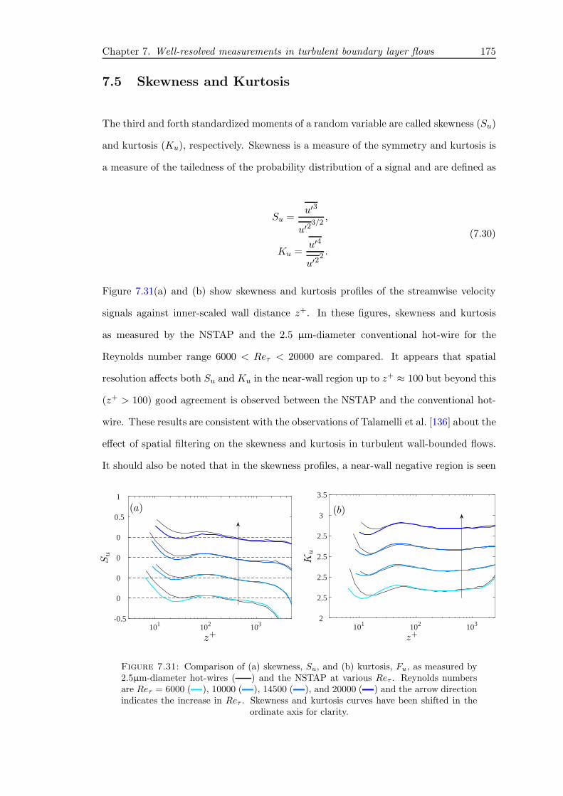
Chapter 7. Well-resolved measurements in turbulent boundary layer flows 175
7.5 Skewness and Kurtosis
The third and forth standardized moments of a random variable are called skewness (Su)
and kurtosis (Ku), respectively. Skewness is a measure of the symmetry and kurtosis is
a measure of the tailedness of the probability distribution of a signal and are defined as
Su =u′3
u′23/2
,
Ku =u′4
u′22 .
(7.30)
Figure 7.31(a) and (b) show skewness and kurtosis profiles of the streamwise velocity
signals against inner-scaled wall distance z+. In these figures, skewness and kurtosis
as measured by the NSTAP and the 2.5 µm-diameter conventional hot-wire for the
Reynolds number range 6000 < Reτ < 20000 are compared. It appears that spatial
resolution affects both Su and Ku in the near-wall region up to z+ ≈ 100 but beyond this
(z+ > 100) good agreement is observed between the NSTAP and the conventional hot-
wire. These results are consistent with the observations of Talamelli et al. [136] about the
effect of spatial filtering on the skewness and kurtosis in turbulent wall-bounded flows.
It should also be noted that in the skewness profiles, a near-wall negative region is seen
101 102 103-0.5
0
0
0
0
0.5
1
Su
z+
(a)
101 102 1032
2.5
2.5
2.5
2.5
3
3.5
Ku
z+
(b)
Figure 7.31: Comparison of (a) skewness, Su, and (b) kurtosis, Fu, as measured by2.5µm-diameter hot-wires ( ) and the NSTAP at various Reτ . Reynolds numbersare Reτ = 6000 ( ), 10000 ( ), 14500 ( ), and 20000 ( ) and the arrow directionindicates the increase in Reτ . Skewness and kurtosis curves have been shifted in the
ordinate axis for clarity.

Chapter 7. Well-resolved measurements in turbulent boundary layer flows 176
in the NSTAP results for all the Reynolds numbers, while the conventional hot-wire
wires cannot resolve this due to spatial filtering.
Figure 7.32(a) and (b) show the evolution of the skewness factor with Reτ against inner-
scaled and outer-scaled wall-distance, respectively. Similar plots are shown in figure
7.33(a) and (b) for the kurtosis. In the near-wall region a very weak dependency on
Reτ in the Reynolds number range of this study is observed especially in the skewness
profiles. Metzger and Klewicki [85] and Inoue et al. [50] have reported a similar trend
over a much larger Reynolds number range. Metzger and Klewicki [85] related this
trend to the growing influence of the large-scales with Reτ . They also reported that the
negative peak present in the skewness profiles of low Reτ number data is not present
for the high Reτ data of atmospheric surface layer. Considering the weak dependence of
the near-wall trend seen here and also noting that the spatial filtering and Reτ exhibit
similar near wall effects in the skewness and kurtosis profiles, care must be taken about
the spatial resolution when studying such Reτ trends. Further away from the wall for
z+ > 200 a reasonable collapse can be seen with inner scaling for both skewness and
kurtosis before the wake region, where a clear Reτ trend occurs. In contrast, with the
outer-scaling no clear collapse is seen for the skewness profiles in the Reynolds number
range Reτ = 6000 − 20000 while kurtosis profiles show some degree of collapse in the
range 0.03 < z/δ < 1.
The non-Gaussian characteristics of the turbulent boundary layer are demonstrated in
figures 7.32 and 7.33 especially in the near-wall region. In the logarithmic region, skew-
ness appears to asymptote to -0.1 which is near 0 (= Gaussian standard for skewness),
and kurtosis maintains a magnitude of ∼ 2.7 which is near 3 (=Gaussian standard for
kurtosis). The drastic deviation from Gaussian standard of the skewness and kurtosis
profiles near the edge of the boundary layer is due to the frequent low speed fluctuations
associated with the intermittent turbulent/non-turbulent interface.

Chap
ter7.
Well-reso
lvedmeasurem
ents
inturbu
lentboundary
layer
flows
177
101 102 103 104
-1.5
-1
-0.5
0
0.5
1
10 100-0.1
0
0.1
0.2
0.3
0.4Su
z+
(a)
10-3 10-2 10-1 100
-1.5
-1
-0.5
0
0.5
1
z/δ
(b)
Figure 7.32: Skewness profiles for various Reynolds numbers against (a) inner-scaled wall-distance z+ and (b) outer-scaled wall-distance z/δ. Theinset in (a) depicts an enlarged version of skewness for 4 < z+ < 500. Colour code corresponds to those shown in figure 7.31. Arrows’ direction
indicates increase in the Reτ .
101 102 103 1042
2.5
3
3.5
4
4.5
10 1002.4
2.6
2.8
Ku
z+
(a)
10-3 10-2 10-1 1002
2.5
3
3.5
4
4.5
z/δ
(b)
Figure 7.33: Kurtosis profiles for various Reynolds numbers against (a) inner-scaled wall-distance z+ and (b) outer-scaled wall-distance z/δ. Theinset in (a) depicts an enlarged version of skewness for 4 < z+ < 600. Colour code corresponds to those shown in figure 7.31. Arrows’ direction
indicates increase in the Reτ .

Chapter 7. Well-resolved measurements in turbulent boundary layer flows 178
7.6 Turbulent energy dissipation rate and Kolmogrov scale
characteristics
The smallest, dissipative eddies in turbulence are characterised by Kolmogrov scales as
seen in §7.3.2. These scales depend only on the turbulent energy dissipation rate (ǫ) and
viscosity (ν). Kolmogrov length scale (η) and velocity scale (vη) depend on ǫ and ν as
η =
(ν3
ǫ
)1/4
, (7.31)
and
vη = (νǫ)1/4 . (7.32)
Here we attempt to analyse η and vη in turbulent boundary layers using our well-resolved
single velocity component measurements. To estimate these, an estimate of ǫ must first
be found. One approach is to assume local isotropy which allows ǫ to be determined
from integration of the one-dimensional dissipation spectrum D(kx) (Townsend [140])
ǫ = 15ν
∫ ∞
0D(kx)dkx = 15ν
∫ ∞
0k2xφuudkx. (7.33)
Using equation 7.33 leads to large errors if the velocity signals are contaminated with
high frequency noise, or if spatial and/or temporal resolution are limiting factors since
the multiplication of k2x amplifies the high frequency end of the spectra, which do not
amount to much energy in the turbulence intensity yet contribute to a significant portion
of the energy dissipation rate. Figure 7.34(a) shows the inner-scaled premultiplied one-
dimensional dissipation spectra against inner-scaled wave-number at z+ = 15 for the
experimental data as well as DNS data at various Reynolds numbers, in the range
Reτ = 550 − 5200 for DNS and Reτ = 6000 − 20000 for the experiment. Dissipation
spectra are premultiplied to allow for visual integration in the semi-logarithmic plot. The

Chapter 7. Well-resolved measurements in turbulent boundary layer flows 179
10-2 10-1
×10-3
0
0.5
1
1.5
k+x
ν2kxD/u
4 τ(a)
102 103 104
×10-3
0
0.5
1
1.5
f(Hz)
(b)
Figure 7.34: Inner normalised premultiplied dissipation spectra ν2kxD/u4τ against (a)
Inner normalised streamwise wave-number k+x and (b) frequency (for the experimentaldata only). : NSTAP-Reτ = 6000 , : NSTAP-Reτ = 10000 , : NSTAP-Reτ = 14500, : NSTAP-Reτ = 20000, : DNS channel-Reτ = 5200 [67], :DNS boundary layer δ+99 = 1990 [128], : DNS channel-Reτ ≈ 2000 [41], : DNS
channel-Reτ ≈ 550 [41]. The arrow indicates increase in the Reτ .
experimental spectra appear to be noise free and the majority of the motions contributing
to the dissipation rate are resolved.
An obvious increasing trend with Reτ in the high wave-number end of the DNS spectra
is seen. The experimental data however do not exhibit a clear trend. It should be noted
that these spectra represent very high frequency phenomena, in the range 1 < f < 30
kHz in our measurements (figure 7.34(b)), wherein anemometry sensors are known to
amplify or attenuate energy [49]. Although owing to the very high frequency response of
the NSTAP compared to the conventional hot-wires (∼ 200 kHz compared to ∼ 50 kHz
based on the electronic testing) this temporal effect is expected to be minimal in our
measurements, careful assessment of NSTAP results in this frequency range is required,
which is out of the scope of this study. Therefore, we cannot rely on the Reτ trend seen
in the experimental dissipation spectra of figure 7.34.
Figure 7.35 shows the inner-scaled energy dissipation rate ǫ+ against inner-scaled wall-
distance z+ for the experiments obtained using equation 7.33. The inner-scaling collapses
the profiles in the near-wall and log regions, while a Reτ dependence is seen in the

Chapter 7. Well-resolved measurements in turbulent boundary layer flows 180
outer region. It should be noted that the logarithmic scaling of the ordinate artificially
improves the collapse in the near-wall region. Also shown in the figure is the relation
ǫ+ = 1/κz+. (7.34)
Equation 7.34 follows the assumption that at sufficiently high Reynolds number, there
is an intermediate region between inner and outer layers where the transport terms in
the kinetic energy equation are small compared with production, so that in this region
production and dissipation are approximately in balance, p ≈ ǫ (Hinze [39]). Using
p = −uwdU
dz≈ u2τ
dU
dz, U/uτ = 1/κ log(zuτ/ν) + B, and p ≈ ǫ leads to equation 7.34.
It is noted that this estimate is expected to hold only for the logarithmic region based
on the mentioned assumptions. However, it can be seen that the agreement between
our experimental data and equation 7.34 in the logarithmic region is not particularly
convincing. This might stem from the assumption of isotropy in the logarithmic region,
or the balanced production and dissipation.
101 102 103 10410-5
10-4
10-3
10-2
10-1
ǫ+ = 1/κz+
z+
ǫ+
Figure 7.35: Inner-scaled dissipation rate ǫ+ against inner-scaled wall-distance z+ forvarious Reτ . The arrow indicates increase in Reτ . Dashed line corresponds to equation
7.34.

Chapter 7. Well-resolved measurements in turbulent boundary layer flows 181
101 102 103 1041
3
5
7
9
η+ = (κz+)1/4
z+
η+
Figure 7.36: Inner-scaled Kolmogrov’s length scale η+ against inner-scaled wall-distance z+ for various Reτ . The arrow indicates increase in Reτ . Dashed line corre-
sponds to equation 7.35.
Using equations 7.31, 7.32, and 7.34 yields
η+ = (κz+)1/4, (7.35)
and
v+η = (κz+)−1/4, (7.36)
for Kolmogrov’s length and velocity scales.
Figure 7.36 and 7.37 show the inner-scaled Kolmogrov’s length and velocity scales ob-
tained using equations 7.33, 7.31, and 7.32 across the boundary layer for the experimental
data. The inner-scaling leads to reasonable collapse in the near-wall and logarithmic re-
gions, while the profiles exhibit Reτ trends in the outer region. Similar to the dissipation

Chapter 7. Well-resolved measurements in turbulent boundary layer flows 182
101 102 103 1040
0.1
0.2
0.3
0.4
0.5
v+η = (κz+)−1/4
z+
v+η
Figure 7.37: Inner-scaled Kolmogrov’s velocity scale v+η against inner-scaled wall-distance z+ for various Reτ . The arrow indicates increase in Reτ . Dashed line corre-
sponds to equation 7.36.
rate, the approximate power law relations do not show convincing agreement with the
experiments in the logarithmic region.
7.7 Summary and conclusions
A Nano-Scale Thermal Anemometry Probe (NSTAP) was used to measure the stream-
wise velocity fluctuations in turbulent boundary layer flows in the Reynolds number
range Reτ = 6000−20000 with a unique inner-scaled sensor length range l+ = 2.4−3.5.
First and second order turbulence statistics where compared to those measured by con-
ventional hot-wires and very good agreement was seen in the logarithmic and outer
regions where the effect of sensor spatial resolution is minimal. Furthermore, in the
near-wall region where conventional hot-wires fail to resolve the smallest scales of mo-
tion, the NSTAP results provide useful insight. It was shown that in the near-wall region
the streamwise turbulence intensity normalised with uτ (u2+) increases monotonically
with Reτ in the Reynolds number range of the experiments, and the near-wall peak

Chapter 7. Well-resolved measurements in turbulent boundary layer flows 183
in u2+ was seen to follow a logarithmic relation with Reτ . Moreover, profiles of u2+
against outer-scaled wall-distance z/δ in the inertial sublayer and outer layer collapsed
well, following a logarithmic decay of the form u2+ = B1 −A1 log(z/δ), with A1 = 1.26
and B1 = 1.95 in the inertial sublayer. A logarithmic curve fit was proposed for the
intermediate region of the turbulence intensity profile. Extrapolating the fit, showed a
clear outer peak at Reynolds number of O(106) exhibiting a very good agreement against
atmospheric surface layer data.
Streamwise energy spectra were investigated in the near-wall region, inertial sublayer,
and outer region. When spectra of various Reynolds numbers were compared at fixed
viscous-scaled wall distances, in the near-wall region (z+ ≤ 300) inner-scaling collapsed
the spectra for small and moderate wavelengths (large and moderate wavenumbers),
while the spectra exhibited an increasing trend with Reτ for large wavelengths. These
large-scale energy contributions in the u-spectra, which increase with Reτ , are attributed
to the footprint of large-scale features in the inertial sublayer, and are responsible for the
growth of the turbulence intensity inner peak with Reτ . In the inertial sublayer, energy
spectra scale both with z and δ, therefore exhibiting a mixed scaling. A low wavenumber
region of overlap in the spectra was found as a function of z/δ over which spectra have
a quasi-plateau. It was shown that the magnitude of this quasi-plateau (named A∗1 in
analogy to Perry’s A1) asymptotes to 1.4 ± 0.1 when z/δ → 0 using our NSTAP data
together with previously available atmospheric surface layer data. Moreover, the energy
spectra were integrated and a relation of the form u2+ = B∗1(z/δ)−A∗
1(z/δ) log(z/δ) for
the streamwise turbulence intensity was derived suggesting that the Perry’s constant A1
is a function of z/δ given here as A∗1(z/δ). Spectrograms were examined and it was shown
that the energetic outer site that appears as an outer peak in the moderate Reynolds
numbers Reτ = 6000 − 14500 grows into a small region of plateau at Reτ = 20000
and 25000, which signals emergence of the k−1x region at Reynolds numbers higher than
25000. It is noted that given the observed outer-scaling similarity, it should not be
expected to see a k−1x region anywhere in the boundary layer above outer-scaled wall-
distance z/δ ≈ 0.01 even at a very high Reynolds number.
Chapter 7. Well-resolved measurements in turbulent boundary layer flows 184
We used a local isotropy assumption to determine energy dissipation rate from integra-
tion of the one-dimensional dissipation spectra across the boundary layer, which allowed
us to calculate Kolmogrov’s length and velocity scales. Good collapse of all the above
parameters was seen with inner-scaling in the logarithmic region. Using two assumptions
of local isotropy and balance of turbulence energy production and dissipation to calcu-
late the dissipation rate did not seem to give a convincing agreement in the logarithmic
region, which might be due to invalidity of either of these assumptions. However, draw-
ing conclusion for turbulent energy dissipation based on one-dimensional data might not
be correct.

Chapter 8
Conclusions and future work
8.1 Conclusions
The application of sub-miniature hot-wires in high Reynolds number turbulent wall-
bounded flows is thoroughly examined in this study. Such probes are increasingly re-
quired for high Reynolds number turbulent flow measurements. Challanges regarding
the operation of these hot-wires in constant temperature mode is investigated in Chap-
ter 4. Moreover, in high Reynolds number turbulent flows, researchers are inclined to
relax the accepted length-to-diameter ratio (required to avoid end-conduction effects)
in order to achieve better spatial resolution (see e.g. Morrison et al. [96], Li et al. [71]
and Vallikivi [144]). Therefore, the effect of end-conduction in constant temperature
hot-wire anemometry is revisited in Chapter 5.
A Nano-Scale Thermal Anemometry Probe (NSTAP) with a sensing length l = 60µm
is used to measure velocity fluctuations in turbulent boundary layers in the Reynolds
number range Reτ = 6000 − 20000 with the probe viscous-scaled length of the range
l+ = 2.4 − 3.5. A modified Melbourne University Constant Temperature Anemometer
(MUCTA) as well as a Dantec Streamline system are used to operate nearly a dozen
NSTAP probes at various Reynolds numbers, and their results are compared with those
of conventional 2.5µm-diameter hot-wires in Chapter 6. The NSTAPs that compare
185

Chapter 8. Conclusions and future work 186
favourably against conventional hot-wires in the outer region of the turbulence intensity
profiles are noted as reliable and their data are used for further analysis of high Reynolds
number turbulent flows with a unique spatial resolution range of l+ = 2.4−3.5 in Chapter
7.
The most important findings of this study are: Proper filtering of the second stage amplifier is required in order for MUCTA to
perform the square-wave test with a sub-miniature wire without damaging the
wire due to instability. Cold resistance of sub-miniature wires are usually one order of magnitude greater
than the conventional wires (O(100) against O(10)). Top-of-bridge resistors’ values
in MUCTA, which are ideal for conventional wires, were found to be too small for
NSTAP as even small electric current fluctuations can damage the sensor. By
changing those resistors to 10 times the original values, the electrical fluctuations
were dampened by a factor of 3 (as predicted by a theoretical model) and the
NSTAP probes were successfully operated by the MUCTA. In Chapter 5, a theoretical model for the hot-wire-CTA system transfer function
was developed that takes into account the axial heat conduction for the hot-wire
filament, the stub’s and prong’s effects, and the asymmetry in the boundary condi-
tions of the wire filament. The model predicts both positive and negative steps in
the overall transfer function of the system to the velocity fluctuations with different
combinations of probe geometry and conductivity parameters. It should be noted
that the presence of positive steps in the transfer function of the hot-wire-CTA sys-
tem leads to amplification of the measured energy and turbulence intensity, while
negative steps result in attenuation of energy meaning that both amplification and
attenuation of energy due to end conduction errors are possible. It was observed
that for the length-to-diameter ratios of 100 and 200, positive steps are more likely
to exist in the system transfer function, while for the length-to-diameter ratio of
50, negative steps are dominant.

Chapter 8. Conclusions and future work 187 Experiments (using conventional hot-wires) were conducted to verify the model
with regards to the end-conduction effect, and results were in accordance with
the theoretical model predictions confirming that both positive and negative low
frequency steps were possible for hot-wires of different length-to-diameter ratios.
These effects extend further away from the wall compared to those seen in spatial
resolution effects and start from lower frequencies (∼ 10 Hz) in the energy spectra. Nearly a dozen NSTAP probes together with a 2.5 µm-diameter hot-wire were used
to measure streamwise velocity fluctuations in the HRNBLWT facility at various
Reynolds numbers. Comparison of the mean velocity profiles as measured by the
NSTAPs and the hot-wire exhibited very good agreement between all the NSTAPs
and the hot-wire. However, comparison of the turbulence intensity profiles revealed
discrepancies between some of the NSTAPs and the hot-wires in the logarithmic
and outer region of the turbulence intensity profiles, where based on the study
of Hutchins et al. [47], minimal difference between wires of different lengths is
expected. Moreover, the observed variations between NSTAPs and the hot-wires
were not consistent neither in size nor in sign. In fact both magnification and
attenuation of turbulence intensity were observed in different NSTAP probes when
compared to the hot-wires. An investigation of the premultiplied energy spectra
revealed that the energy deviation in the NSTAPs, which were in conflict with
the hot-wires in the outer region of the turbulence intensity, initiated at very low
frequencies (∼ 10 Hz). Measurements with both the MUCTA and the Dantec Streamline contained reli-
able NSTAPs and unreliable NSTAPs. This rules out the effect of the anemometer
in the conflicting behaviours of some NSTAPs. Reliable NSTAP is referred to an
NSTAP probe that agrees with the 2.5 µm-diameter hot-wire in the logarithmic
and outer region of the turbulence intensity profile and the rest of the NSTAP
probes are referred to as unreliable NSTAPs. The mean velocity and the turbu-
lence intensity profiles measured by the reliable NSTAPs were averaged to obtain
smooth, averaged NSTAP results, which compared well against hot-wires.

Chapter 8. Conclusions and future work 188 Results of the reliable NSTAPs showed that in the near-wall region the streamwise
turbulence intensity normalised with uτ (u2+) increases monotonically with Reτ
in the Reynolds number range of the experiments, and the near-wall peak in u2+
was seen to follow a logarithmic relation with Reτ . Profiles of u2+ against outer-scaled wall-distance z/δ in the inertial sublayer (or
logarithmic layer) and outer layer collapsed well, following a logarithmic decay of
the form u2+ = B1 − A1 log(z/δ), with A1 = 1.26 and B1 = 1.95 in the inertial
sublayer. A logarithmic curve fit was proposed for the intermediate region of the turbulence
intensity profile (100 ≤ z+ ≤ 3Re1/2τ ). Extrapolating the fit to higher Reynolds
number showed a clear outer peak at Reynolds number Reτ ∼ O(106) exhibiting a
very good agreement against the atmospheric surface layer data of Metzger et al.
[84]. When energy spectra at various Reynolds numbers and fixed viscous-scaled wall
distances were compared in the near-wall region (z+ ≤ 100), inner-scaling collapsed
the spectra for small and moderate wavelengths (large and moderate wavenum-
bers), while the spectra exhibited an increasing trend with Reτ for large wave-
lengths. These large-scale energy contributions in the u-spectra, which increase
with Reτ , are attributed to the footprint of large-scale features in the inertial sub-
layer, and are responsible for the growth of the turbulence intensity inner peak
with Reτ . In the spatial inertial sublayer, energy spectra scale both with z and δ, therefore
exhibiting a mixed scaling. A low wavenumber region of overlap in the spectra was
found as a function of z/δ over which spectra have a quasi-plateau. The magnitude
of this quasi-plateau asymptotes to 1.4 ± 0.1 when z/δ → 0 according to our
NSTAP data and previously available atmospheric surface layer data. Because
of this asymptotic behaviour it is expected that a low wavenumber k−1x region

Chapter 8. Conclusions and future work 189
appears at extremely high Re in which the logarithmic region extends towards the
wall for asymptotically small z/δ. Examination of spectrograms revealed that the energetic outer site that appears as
an outer peak in the moderate Reynolds numbers Reτ = 6000− 14500, grows into
a small region of plateau at Reτ = 20000 and 25000, which signals the emergence
of the k−1x region at Reynolds numbers higher than 25000. This plateau region
in the spectrograms is associated with the low wavenumber quasi-plateau region
described in the one-dimensional energy spectra.
8.2 Future work
Although most of the NSTAP probes proved to be reliable, some of them yielded in-
consistent turbulent energy results, while their mean velocity results were in excellent
agreement with conventional hot-wires. Hence, these malfunctions are considered as
dynamic rather than static. We were able to identify the reliable NSTAPs by comparing
them against the results of conventional hot-wires. However, discovering a procedure to
pinpoint the reliable NSTAPs as part of the manufacturing process can be valuable. To
this end, one needs to find the reason(s) for these anomalous behaviours. NSTAPs are
manufactured using MEMS fabrication techniques, the accuracy of which is known to
deteriorate as the dimensions decrease [36]. Therefore, we speculate that the observed
inconsistent results could be due to inconsistency in the sensor’s dimensions. A system-
atic study of the physical properties of each NSTAP probe, i.e. all dimensions of the
sensing part, stubs, and prongs as well as the cold resistance of the probes, before using
them in high Reynolds number turbulence measurements, can enable us to discover a
correlation between the probe’s principal dimensions and the errors in the results. It is
noted that the thickness of the sensor as well as its length and width are important, and
given the minuscule size and fragility of the NSTAPs, an accurate measurement of all
the dimensions is challenging. Finding such a correlation provides a screening scheme

Chapter 8. Conclusions and future work 190
by which the reliable NSTAPs can be identified as part of the manufacturing process,
and also helps to improve the probe design by modifying the dimensions accordingly.
Since the problems found with some of the NSTAP probes are dynamic, they might be
related to the forming of hot spots on the sensors during the constant temperature opera-
tion as reported by Perry et al. [114]. They showed that hot spots can affect the dynamic
properties of hot-wires, leading to large measurement errors. To determine whether hot
spots are causing the above-mentioned problems, nano-scale thermal imaging may be
exploited to acquire temperature distribution of the probes during the operation, which
in turn can provide valuable information with regards to the axial conduction related
errors discussed in Chapter 5.
Thanks to their smaller size compared to conventional hot-wires, NSTAPs are suitable
for the study of high Reynolds number wall-bounded turbulence in the near-wall re-
gion. They have been utilized in the Superpipe and HRTF at Princeton University and
the HRNBLWT at the University of Melbourne, among other facilities. Recently, con-
struction of a long pipe in the framework of the Center for International Cooperation
in Long Pipe Experiments (CICLoPE) at the University of Bologna has been finalized.
Although, the main purpose of the construction of the CICLoPE was the viability of re-
solving the smallest scales using conventional measurement tools, recent published data
from this facility revealed spatial resolution issues in the near-wall region at Reynolds
numbers higher than Reτ ≈ 5000 [105]. Utilizing NSTAP allows us to overcome this
spatial resolution issue up to the highest Reynolds number attainable in the CICLoPE.
As a screening scheme for identifying the reliable NSTAPs is not available yet, in order to
avoid publishing discrepant data, carrying out multiple measurements at each Reynolds
number using various NSTAP probes is required, similar to those taken in the course of
this thesis and elaborated in Chapter 6.
Despite its importance to wall-bounded turbulence, there is currently a lack of high
Reynolds number data of two-component turbulence measurements. Baidya [5] utilized
custom-made miniature cross-wire sensors in boundary layer turbulent flows. However,

Chapter 8. Conclusions and future work 191
this study was limited to Reynolds numbers below Reτ = 10000 to avoid spatial resolu-
tion filtering. In the present study we were limited to using single component NSTAP
probes to measure the streamwise velocity fluctuating component. Recently, improve-
ments have been made towards the development of x-NSTAPs [28]. x-NSTAPs, similar
to conventional cross-wire sensors, are capable of measuring two velocity components in
the sensor’s plane with nearly one order of magnitude smaller size in every dimension.
Therefore, they can be used in high Reynolds number facilities such as HRNBLWT and
CICLoPE to measure all components of turbulence intensity as well as Reynolds shear
stress up to very high Reynolds numbers with exceptional spatial resolution.

Appendix A
Temperature correction
The governing equations for a hot-wire-CTA system (e.g. equation 2.36a in Brunn [14])
show that the output voltage of the system not only is a function of the flow velocity past
the wire but also the ambient temperature. Therefore, if the temperature of the flow
changes significantly during the calibration or the measurement, the regular calibration
where the voltage of the system is calibrated against the flow velocity measured by
a Pitot-static tube might lead to errors in the results. Perry [116] suggests that if
the temperature is within ±0.5C throughout the calibration and measuring procedure,
temperature corrections are not necessary. This is fulfilled for the measurements at U∞ =
20 ms−1 in the HRNBLWT, however for higher velocities the temperature variation
during the calibration is higher. This is shown in figure A.1 where the flow temperature
is demonstrated versus velocity for pre- and post-calibrations for the measurements made
at free stream velocities 20, 30, and 40 ms−1. Two types of temperature variations are
recognised for all the cases:
1. Temperature variation during each calibration which is ∆T ≈ 0.5C, ∆T ≈ 1.5C,
and ∆T ≈ 3C for U∞ = 20 ms−1, U∞ = 30 ms−1 , and U∞ = 40 ms−1, respec-
tively.
2. Temperature variation between pre- and post-calibrations when same velocities
are compared.
192

Appendix A. Temperature correction 193
0 5 10 15 20 2526.5
27
27.5
28
U(m/s)
T(C)
(a)
0 5 10 15 20 25 30 3528
28.5
29
29.5
30
U(m/s)
(b)
0 10 20 30 40 50
28
29
30
31
32
33
U(m/s)
T(C)
(c)
Figure A.1: Temperature versus free stream velocity in the HRNBLWT during thecalibration; : pre-calibration, : post-calibration. (a) Calibration for a measure-ment made at U∞ = 20 ms−1 (b) Calibration for a measurement made at U∞ = 30 ms−1
(c) Calibration for a measurement with made at U∞ = 40 ms−1.
The latter is dealt with by using the correction scheme proposed by Talluru et al.
[137]. However a temperature correction scheme might be required for the cases where
temperature variations during the calibrations are higher than 0.5C since the calibration
curves might need to be dewarped for temperature changes.
Several temperature correction methods have been proposed in the literature (see e.g.
Abdel-Rahman et al. [1], Bearman [11], Benjamin and Roberts [12], Brunn [14], Hult-
mark and Smits [42], Tropea et al. [141]). Here we first use the correction by Hultmark
and Smits [42]. In this method, similar to other analytical correction techniques, the
raw voltage signal from the hot-wire-CTA system (without any signal conditioning) is
required. This is available with the Dantec Streamline anemometer where the gain and
offset in the signal conditioning stage are known. However the numerical values for the

Appendix A. Temperature correction 194
100 101 102 103 104 1055
10
15
20
25
30
z+
U+
(a)
100 101 102 103 104 1050
2
4
6
8
10
z+
u2+
(b)
Figure A.2: Effect of temperature correction scheme proposed by Hultmark and Smits[42] for data acquired by NSTAP operated by Dantec Streamline in the HRNBLWT atU∞ = 20 ms−1. : with temperature correction, : without temperature correction.(a) Streamwise mean velocity (U) and (b) variance of streamwise velocity component
(u2).
100 101 102 103 104 1055
10
15
20
25
30
35
z+
U+
(a)
100 101 102 103 104 1050
2
4
6
8
10
12
z+
u2+
(b)
Figure A.3: Effect of temperature correction scheme proposed by Hultmark and Smits[42] for data acquired by NSTAP operated by Dantec Streamline in the HRNBLWT atU∞ = 30 ms−1. : with temperature correction, : without temperature correction.(a) Streamwise mean velocity (U) and (b) variance of streamwise velocity component
(u2).
gain and offset are unknown for the MUCTA. Therefore using this method is not viable
for the data obtained using the MUCTA. Figure A.2 shows the corrected and uncorrected
data acquired by NSTAP operated by the Dantec Streamline CTA in the HRNBLWT
at free stream velocity U∞ = 20 ms−1. As expected the effect of the correction on
the results is negligible at this velocity. This correction was applied to another dataset
acquired at U∞ = 30 ms−1 in the HRNBLWT with the same anemometry system and
the results are shown in figure A.3. It can be seen that at U∞ = 30 ms−1 the effect
of temperature correction is negligible as well. Hence we conclude that no temperature

Appendix A. Temperature correction 195
31 31.5 32 32.5 334.22
4.24
4.26
4.28
4.3
4.32
4.34
T (C)
E(V
)
40.15 40.2 40.25 40.3 40.35 40.4 40.45 40.54.22
4.24
4.26
4.28
4.3
4.32
4.34
U(ms−1)
Figure A.4: (a) Hot-wire-CTA voltage versus the ambient temperature. (b) Hot-wire voltage versus the free stream velocity measured by a Pitot-static tube during the
measurement as part of the correction scheme proposed by Talluru et al. [137].
correction is required for the data obtained at U∞ = 20 and 30 ms−1.
Measurements conducted at U∞ = 40 ms−1 in the HRNBLWT in this study were made
with conventional 2.5 µm-diameter hot-wires operated with the MUCTA. Therefore
using the above mentioned correction scheme was not possible for these measurements
as the raw voltage signal of the hot-wire-CTA system was not retrievable. To overcome
this problem we use the trace of the system voltage (conditioned signal) in the free
stream that is obtained as part of the correction procedure proposed by Talluru et al.
[137]. In this procedure the hot-wire is traversed into the free stream at regular intervals
during the course of the measurement and single recalibration points are obtained. If
we assume that the temperature drift is the only reason for the drift of the hot-wire-
CTA system voltage, we can find a correlation between the voltage and the ambient
temperature. This is shown in figure A.4(a) which shows a near linear relation between
the hot-wire-CTA system voltage and the ambient temperature. At this stage one might
suspect that the voltage drift can occur due to slight changes in the speed of the tunnel
fan. This is examined by plotting the hot-wire-CTA system voltage versus the velocity
measured by the Pitot-static tube placed in the free stream as shown in figure A.4(b).
It can be seen that there is no correlation between the free stream velocity and the
hot-wire-CTA system voltage. Therefore one can assume that the drift between the
pre- and post-calibration voltages is due to the temperature drift only and to a linear
approximation use dE/dT = (Epost − Epre)/(Tpost − Tpre) for each calibration point

Appendix A. Temperature correction 196
100 101 102 103 104 1055
10
15
20
25
30
35
z+
U+
(a)
100 101 102 103 104 1050
2
4
6
8
10
z+
u2+
(b)
Figure A.5: Effect of the linear temperature correction scheme for data acquired bya 2.5 µm-diameter hot-wire operated with the MUCTA in the HRNBLWT at U∞ =40 ms−1. : with temperature correction, : without temperature correction. (a)Streamwise mean velocity (U) and (b) variance of streamwise velocity component (u2).
(speed) in both pre- and post-calibration curves. Then we use these voltage sensitivities
(obtained for all the calibration points) to correct the voltages in the calibration curves
using a linear relation as
Ecorr = E +dE
dT(T − Tmeas) (A.1)
where E and T are the hot-wire-CTA system voltage and the ambient temperature for
each calibration point, respectively. Tmeas is the average of temperature during the
course of the actual measurement. Using this procedure one can correct the calibration
curves for temperature drifts. As the reference temperature is considered to be the
(averaged) temperature of the actual measurement, the voltages of the measurement are
not required to be corrected. This correction was implemented for the data obtained by
a 2.5 µm-diameter hot-wire operated with the MUCTA in the HRNBLWT (for which the
hot-wire voltage trace at the free stream was shown in figure A.4). The streamwise mean
velocity (U) profile and the variance of the streamwise velocity component (u2) before
and after this correction are shown in figure A.5. It can be seen that the correction leads
to larger differences in both mean velocity and turbulence intensity profiles compared
to the measurements made at U∞ = 20 ms−1 and 30 ms−1 (after using the temperature
correction) shown in figures A.2 and A.3, respectively.

Bibliography
[1] A. Abdel-Rahman, C. Tropea, P. Slawson, and A. Strong. On temperature com-
pensation in hot-wire anemometry. Journal of Physics E: Scientific Instruments,
20(3):315, 1987.
[2] J. Ahn, J. H. Lee, J. Lee, J.-h. Kang, and H. J. Sung. Direct numerical simulation
of a 30R long turbulent pipe flow at Reτ = 3008. Physics of Fluids, 27(6):065110,
2015.
[3] P. H. Alfredsson, A. Segalini, and R. Orlu. A new scaling for the streamwise
turbulence intensity in wall-bounded turbulent flows and what it tells us about
the outer peak. Physics of fluids, 23(4):041702, 2011.
[4] G. Arwatz, C. Bahri, A. J. Smits, and M. Hultmark. Dynamic calibration and
modeling of a cold wire for temperature measurement. Measurement Science and
Technology, 24(12):125301, 2013.
[5] R. Baidya. Multi-component velocity measurements in turbulent boundary lay-
ers. PhD thesis, University of Melbourne, Department of Mechanical Engineering,
2016.
[6] S. C. Bailey, G. J. Kunkel, M. Hultmark, M. Vallikivi, J. P. Hill, K. A. Meyer,
C. Tsay, C. B. Arnold, and A. J. Smits. Turbulence measurements using a
nanoscale thermal anemometry probe. Journal of Fluid Mechanics, 663:160–179,
2010.
197

Bibliography 198
[7] T. Banerjee and G. Katul. Logarithmic scaling in the longitudinal velocity variance
explained by a spectral budget. Physics of Fluids, 25(12):125106, 2013.
[8] G. Barenblatt. Scaling laws for fully developed turbulent shear flows. part 1. basic
hypotheses and analysis. Journal of Fluid Mechanics, 248:513–520, 1993.
[9] G. Barenblatt, A. Chorin, and V. Prostokishin. Scaling laws for fully developed
turbulent flow in pipes: Discussion of experimental data. Proc. of the Natl. Acad.
Sci USA, pages 773–776, 1997.
[10] G. I. Barenblatt, A. J. Chorin, and V. Prostokishin. Self-similar intermediate
structures in turbulent boundary layers at large Reynolds numbers. Journal of
Fluid Mechanics, 410:263–283, 2000.
[11] P. W. Bearman. Corrections for the effect of ambient temperature drift on hot-wire
measurements in incompressible flow. DISA inf, (11):25–30, 1971.
[12] S. Benjamin and C. Roberts. Measuring flow velocity at elevated temperature
with a hot wire anemometer calibrated in cold flow. International Journal of Heat
and Mass Transfer, 45(4):703–706, 2002.
[13] Y. Borisenkov, G. Gulitski, M. Kholmyansky, S. Krylov, A. Liberzon, and A. Tsi-
nober. Micro-machined super-miniature hot-film multi-array probe for field ex-
periments with sub-Kolmogorov resolution. Journal of Turbulence, 16(6):525–539,
2015.
[14] H. H. Brunn. Hot-wire anemometry. Oxfor Univ Press, New York, 1995.
[15] J. Carlier and M. Stanislas. Experimental study of eddy structures in a turbulent
boundary layer using particle image velocimetry. Journal of Fluid Mechanics, 535:
143–188, 2005.
[16] D. Chandran, R. Baidya, J. P. Monty, and I. Marusic. Two-dimensional en-
ergy spectra in high Reynolds number turbulent boundary layers. arXiv preprint
arXiv:1705.02103, 2017.

Bibliography 199
[17] K. Chauhan, H. Nagib, and P. Monkewitz. On the composite logarithmic profile
in zero pressure gradient turbulent boundary layers. In 45th AIAA Aerospace
Sciences Meeting and Exhibit, page 532, 2007.
[18] K. A. Chauhan, P. A. Monkewitz, and H. M. Nagib. Criteria for assessing experi-
ments in zero pressure gradient boundary layers. Fluid Dynamics Research, 41(2):
021404, 2009.
[19] C. Chin, N. Hutchins, A. Ooi, and I. Marusic. Use of direct numerical simula-
tion (DNS) data to investigate spatial resolution issues in measurements of wall-
bounded turbulence. Measurement Science and Technology, 20(11):115401, 2009.
[20] C. Chin, N. Hutchins, A. Ooi, and I. Marusic. Spatial resolution correction for
hot-wire anemometry in wall turbulence. Experiments in Fluids, 50(5):1443–1453,
2011.
[21] C. Chin, J. Monty, and A. Ooi. Reynolds number effects in DNS of pipe flow and
comparison with channels and boundary layers. International Journal of Heat and
Fluid Flow, 45:33–40, 2014.
[22] D. Coles. The law of the wake in the turbulent boundary layer. Journal of Fluid
Mechanics, 1(02):191–226, 1956.
[23] G. Comte-Bellot. Hot-wire anemometry. Annual Review of Fluid Mechanics, 8(1):
209–231, 1976.
[24] P. Davidson, T. Nickels, and P.-A. Krogstad. The logarithmic structure function
law in wall-layer turbulence. Journal of Fluid Mechanics, 550:51–60, 2006.
[25] D. B. De Graaff and J. K. Eaton. Reynolds-number scaling of the flat-plate tur-
bulent boundary layer. Journal of Fluid Mechanics, 422:319–346, 2000.
[26] J. C. del Alamo and J. Jimenez. Spectra of the very large anisotropic scales in
turbulent channels. Physics of Fluids, 15(6):L41–L44, 2003.

Bibliography 200
[27] H. L. Dryden, G. Schubauer, W. Mock Jr, and H. Skramstad. Measurements
of intensity and scale of wind-tunnel turbulence and their relation to the critical
Reynolds number of spheres. NACA Technical Report 581, 1937.
[28] Y. Fan, G. Arwatz, T. Van Buren, D. Hoffman, and M. Hultmark. Nanoscale
sensing devices for turbulence measurements. Experiments in Fluids, 56(7):1–13,
2015.
[29] H. Fernholz and P. Finleyt. The incompressible zero-pressure-gradient turbulent
boundary layer: an assessment of the data. Progress in Aerospace Sciences, 32(4):
245–311, 1996.
[30] H. Fernholz, E. Krause, M. Nockemann, and M. Schober. Comparative mea-
surements in the canonical boundary layer at Reδ2 ≤ 6 × 10⁴ on the wall of the
German–Dutch windtunnel. Physics of Fluids, 7(6):1275–1281, 1995.
[31] F. Frenkiel. The influence of the length of a hot wire on the measurements of
turbulence. Physical Review, 75(8):1263, 1949.
[32] F. Frenkiel. Effects of wire length in turbulence investigations with a hot-wire
anemometer. Aeronautical Quarterly, 5(01):1–24, 1954.
[33] P. Freymuth. Feedback control theory for constant-temperature hot-wire
anemometers. Review of Scientific Instruments, 38(5):677–681, 1967.
[34] P. Freymuth. Frequency response and electronic testing for constant-temperature
hot-wire anemometers. Journal of Physics E: Scientific Instruments, 10(7):705,
1977.
[35] W. K. George, L. Castillo, and P. Knecht. Zero-pressure-gradient turbulent bound-
ary layer. Applied Mechanics Reviews, 50:689–730, 1997.
[36] R. Ghodssi and P. Lin. MEMS materials and processes handbook, volume 1.
Springer Science & Business Media, 2011.
[37] M. Head and P. Bandyopadhyay. New aspects of turbulent boundary-layer struc-
ture. Journal of Fluid Mechanics, 107:297–338, 1981.

Bibliography 201
[38] W. Heisenberg. Zur statistischen theorie der turbulenz. Z. Physik, 124:628–657,
1948.
[39] J. O. Hinze. Turbulence. McGraw-Hill, 1975.
[40] M. H. Hites. Scaling of high-Reynolds number turbulent boundary layers in the
National Diagnostic Facility. PhD thesis, Illinois Institute of Technology, 1997.
[41] S. Hoyas and J. Jimenez. Scaling of the velocity fluctuations in turbulent channels
up to Reτ = 2003. Physics of Fluids, 18(1):011702, 2006.
[42] M. Hultmark and A. J. Smits. Temperature corrections for constant temperature
and constant current hot-wire anemometers. Measurement Science and Technol-
ogy, 21(10):105404, 2010.
[43] M. Hultmark, A. Ashok, and A. J. Smits. A new criterion for end-conduction ef-
fects in hot-wire anemometry. Measurement Science and Technology, 22(5):055401,
2011.
[44] M. Hultmark, M. Vallikivi, S. Bailey, and A. Smits. Turbulent pipe flow at extreme
Reynolds numbers. Physical review letters, 108(9):094501, 2012.
[45] M. Hultmark, M. Vallikivi, S. Bailey, and A. Smits. Logarithmic scaling of tur-
bulence in smooth-and rough-wall pipe flow. Journal of Fluid Mechanics, 728:
376–395, 2013.
[46] N. Hutchins and I. Marusic. Evidence of very long meandering features in the
logarithmic region of turbulent boundary layers. Journal of Fluid Mechanics, 579:
1–28, 2007.
[47] N. Hutchins, T. B. Nickels, I. Marusic, and M. Chong. Hot-wire spatial resolution
issues in wall-bounded turbulence. Journal of Fluid Mechanics, 635:103–136, 2009.
[48] N. Hutchins, K. Chauhan, I. Marusic, J. Monty, and J. Klewicki. Towards rec-
onciling the large-scale structure of turbulent boundary layers in the atmosphere
and laboratory. Boundary-Layer Meteorology, 145(2):273–306, 2012.

Bibliography 202
[49] N. Hutchins, J. Monty, M. Hultmark, and A. Smits. A direct measure of the
frequency response of hot-wire anemometers: temporal resolution issues in wall-
bounded turbulence. Experiments in Fluids, 56(1):1–18, 2015.
[50] M. Inoue, R. Mathis, I. Marusic, and D. Pullin. Inner-layer intensities for the flat-
plate turbulent boundary layer combining a predictive wall-model with large-eddy
simulations. Physics of Fluids, 24(7):075102, 2012.
[51] F. Jiang, Y.-C. Tai, C.-M. Ho, R. Karan, and M. Garstenauer. Theoretical and
experimental studies of micromachined hot-wire anemometers. In Electron Devices
Meeting, 1994. IEDM’94. Technical Digest., International, pages 139–142. IEEE,
1994.
[52] J. Jimenez and A. Pinelli. The autonomous cycle of near-wall turbulence. Journal
of Fluid Mechanics, 389:335–359, 1999.
[53] A. V. Johansson and P. H. Alfredsson. Effects of imperfect spatial resolution on
measurements of wall-bounded turbulentbx shear flows. Journal of Fluid Mechan-
ics, 137:409–421, 1983.
[54] M. Jones, T. Nickels, and I. Marusic. On the asymptotic similarity of the zero-
pressure-gradient turbulent boundary layer. Journal of Fluid Mechanics, 616:
195–203, 2008.
[55] B. Kader and A. Yaglom. Spectra and correlation functions of surface layer atmo-
spheric turbulence in unstable thermal stratification. In Turbulence and Coherent
Structures, pages 387–412. Springer, 1991.
[56] G. Katul and C.-R. Chu. A theoretical and experimental investigation of energy-
containing scales in the dynamic sublayer of boundary-layer flows. Boundary-Layer
Meteorology, 86(2):279–312, 1998.
[57] G. G. Katul, A. Porporato, and V. Nikora. Existence of k−11 power-law scaling
in the equilibrium regions of wall-bounded turbulence explained by Heisenberg’s
eddy viscosity. Physical Review E, 86(6):066311, 2012.

Bibliography 203
[58] B. Khoo, Y. Chew, and G. Li. A new method by which to determine the dynamic
response of marginally elevated hot-wire anemometer probes for near-wall velocity
and wall shear stress measurements. Measurement Science and Technology, 6(9):
1399, 1995.
[59] J. Klewicki and R. Falco. On accurately measuring statistics associated with
small-scale structure in turbulent boundary layers using hot-wire probes. Journal
of Fluid Mechanics, 219:119–142, 1990.
[60] J. Klewicki, P. Fife, and T. Wei. On the logarithmic mean profile. Journal of
Fluid Mechanics, 638:73–93, 2009.
[61] S. Kline, W. Reynolds, F. Schraub, and P. Runstadler. The structure of turbulent
boundary layers. Journal of Fluid Mechanics, 30(04):741–773, 1967.
[62] A. N. Kolmogorov. The local structure of turbulence in incompressible viscous
fluid for very large Reynolds numbers. In Dokl. Akad. Nauk SSSR, volume 30,
pages 301–305. JSTOR, 1941.
[63] L. S. Kovasznay. The spectrum of locally isotropic turbulence. Physical Review,
73(9):1115, 1948.
[64] H. Kramers. Heat transfer from spheres to flowing media. Physica, 12(2-3):61–80,
1946.
[65] V. Kulandaivelu. Evolution of zero pressure gradient turbulent boundary layers
from different initial conditions. PhD thesis, University of Melbourne, Department
of Mechanical Engineering, 2012.
[66] G. J. Kunkel and I. Marusic. Study of the near-wall-turbulent region of the high-
Reynolds-number boundary layer using an atmospheric flow. Journal of Fluid
Mechanics, 548:375–402, 2006.
[67] M. Lee and R. D. Moser. Direct numerical simulation of turbulent channel flow
up to Reτ ≈ 5200. Journal of Fluids Mechanics, 774:395–415, 2015.

Bibliography 204
[68] J. Li. Dynamic response of constant temperature hot-wire system in turbulence
velocity measurements. Measurement Science and Technology, 15(9):1835, 2004.
[69] J. Li. The effect of electronic components on the cut-off frequency of the hot-wire
system. Measurement Science and Technology, 16(3):766, 2005.
[70] J. Li. Dynamic response of constant temperature hot-wire systems under various
perturbations. Measurement Science and Technology, 17(10):2665, 2006.
[71] J. Li, B. McKeon, W. Jiang, J. Morrison, and A. Smits. The response of hot
wires in high Reynolds-number turbulent pipe flow. Measurement Science and
Technology, 15(5):789, 2004.
[72] P. Ligrani and P. Bradshaw. Spatial resolution and measurement of turbulence in
the viscous sublayer using subminiature hot-wire probes. Experiments in Fluids,
5(6):407–417, 1987.
[73] P. Ligrani and P. Bradshaw. Subminiature hot-wire sensors: development and use.
Journal of Physics E: Scientific Instruments, 20(3):323, 1987.
[74] C. Marshall, E. Matlis, T. Corke, and S. Gogineni. Ac plasma anemometerchar-
acteristics and design. Measurement Science and Technology, 26(8):085902, 2015.
[75] I. Marusic and G. J. Kunkel. Streamwise turbulence intensity formulation for
flat-plate boundary layers. Physics of Fluids, 15(8):2461–2464, 2003.
[76] I. Marusic, A. Uddin, and A. Perry. Similarity law for the streamwise turbulence
intensity in zero-pressure-gradient turbulent boundary layers. Physics of Fluids, 9
(12):3718–3726, 1997.
[77] I. Marusic, R. Mathis, and N. Hutchins. High Reynolds number effects in wall
turbulence. International Journal of Heat and Fluid Flow, 31(3):418–428, 2010.
[78] I. Marusic, B. McKeon, P. Monkewitz, H. Nagib, A. Smits, and K. Sreenivasan.
Wall-bounded turbulent flows at high Reynolds numbers: Recent advances and
key issues. Physics of Fluids, 22(6):065103, 2010.

Bibliography 205
[79] I. Marusic, J. P. Monty, M. Hultmark, and A. J. Smits. On the logarithmic region
in wall turbulence. Journal of Fluid Mechanics, 716:R3, 2013.
[80] I. Marusic, K. Chauhan, V. Kulandaivelu, and N. Hutchins. Evolution of zero-
pressure-gradient boundary layers from different tripping conditions. Journal of
Fluid Mechanics, 783:379–411, 2015.
[81] R. Mathis, N. Hutchins, and I. Marusic. Large-scale amplitude modulation of the
small-scale structures in turbulent boundary layers. Journal of Fluid Mechanics,
628:311–337, 2009.
[82] R. Mathis, N. Hutchins, and I. Marusic. Scaling of inner and outer regions for flat
plate boundary layers. In Proc. 17th Australasian Fluid Mech. Conf., Auckland,
New Zealand, pages 5–9, 2010.
[83] B. McKeon and J. Morrison. Asymptotic scaling in turbulent pipe flow. Philo-
sophical Transactions of the Royal Society of London A, 365(1852):771–787, 2007.
[84] M. Metzger, B. McKeon, and H. Holmes. The near-neutral atmospheric surface
layer: turbulence and non-stationarity. Philosophical Transactions of the Royal
Society of London A, 365(1852):859–876, 2007.
[85] M. M. Metzger and J. Klewicki. A comparative study of near-wall turbulence in
high and low Reynolds number boundary layers. Physics of Fluids, 13(3):692–701,
2001.
[86] M. M. Metzger, J. Klewicki, K. Bradshaw, and R. Sadr. Scaling the near-wall axial
turbulent stress in the zero pressure gradient boundary layer. Physics of Fluids,
13(6):1819–1821, 2001.
[87] M. Miller, B. Estejab, and S. Bailey. Evaluation of hot-wire spatial filtering cor-
rections for wall turbulence and correction for end-conduction effects. Experiments
in Fluids, 55(5):1735, 2014.
[88] C. B. Millikan. A critical discussion of turbulent flows in channels and circular
tubes. In Proc. 5th Int. Cong. Appl. Mech., volume 386, 1938.

Bibliography 206
[89] S. Mochizuki and F. Nieuwstadt. Reynolds-number-dependence of the maximum
in the streamwise velocity fluctuations in wall turbulence. Experiments in Fluids,
21(3):218–226, 1996.
[90] P. Monkewitz, R. Duncan, and H. Nagib. Correcting hot-wire measurements of
stream-wise turbulence intensity in boundary layers. Physics of Fluids, 22(9):
091701, 2010.
[91] P. A. Monkewitz and H. M. Nagib. Large-Reynolds-number asymptotics of the
streamwise normal stress in zero-pressure-gradient turbulent boundary layers.
Journal of Fluid Mechanics, 783:474–503, 2015.
[92] P. A. Monkewitz, K. A. Chauhan, and H. M. Nagib. Self-consistent high-Reynolds-
number asymptotics for zero-pressure-gradient turbulent boundary layers. Physics
of Fluids, 19(11):115101, 2007.
[93] J. Monty, N. Hutchins, H. Ng, I. Marusic, and M. Chong. A comparison of tur-
bulent pipe, channel and boundary layer flows. Journal of Fluid Mechanics, 632:
431–442, 2009.
[94] J. P. Monty. Developments in smooth wall turbulent duct flows. PhD thesis, Uni-
versity of Melbourne, Department of Mechanical and Manufacturing Engineering,
2005.
[95] S. Morris and J. Foss. Transient thermal response of a hot-wire anemometer.
Measurement Science and Technology, 14(3):251, 2003.
[96] J. Morrison, B. McKeon, W. Jiang, and A. Smits. Scaling of the streamwise
velocity component in turbulent pipe flow. Journal of Fluid Mechanics, 508:99–
131, 2004.
[97] H. Ng, J. Monty, N. Hutchins, M. Chong, and I. Marusic. Comparison of turbulent
channel and pipe flows with varying Reynolds number. Experiments in Fluids, 51
(5):1261–1281, 2011.

Bibliography 207
[98] H. C. Ng. Experiments in smooth wall turbulent channel and pipe flows. PhD
thesis, University of Melbourne, Department of Mechanical Engineering, 2011.
[99] T. Nickels, I. Marusic, S. Hafez, and M. Chong. Evidence of the k−11 law in a
high-Reynolds-number turbulent boundary layer. Physical Review Letters, 95(7):
074501, 2005.
[100] T. Nickels, I. Marusic, S. Hafez, N. Hutchins, and M. Chong. Some predictions of
the attached eddy model for a high reynolds number boundary layer. Philosoph-
ical Transactions of the Royal Society of London A: Mathematical, Physical and
Engineering Sciences, 365(1852):807–822, 2007.
[101] V. Nikora. Origin of the “-1” spectral law in wall-bounded turbulence. Physical
Review Letters, 83(4):734–736, 1999.
[102] M. Oberlack. A unified approach for symmetries in plane parallel turbulent shear
flows. Journal of Fluid Mechanics, 427:299–328, 2001.
[103] R. Orlu and P. H. Alfredsson. Comment on the scaling of the near-wall streamwise
variance peak in turbulent pipe flows. Experiments in Fluids, 54(1):1431, 2013.
[104] R. Orlu, A. Segalini, J. Klewicki, and P. H. Alfredsson. High-order generalisation
of the diagnostic scaling for turbulent boundary layers. Journal of Turbulence, 17
(7):664–677, 2016.
[105] R. Orlu, T. Fiorini, A. Segalini, G. Bellani, A. Talamelli, and P. H. Alfredsson.
Reynolds stress scaling in pipe flow turbulence - first results from CICLoPE. Philo-
sophical Transactions of the Royal Society of London A, 375(2089):20160187, 2017.
[106] J. M. Osterlund. Experimental studies of zero pressure-gradient turbulent boundary
layer flow. PhD thesis, Royal Institute of Technology, Department of Mechanics,
1999.
[107] P. Paranthoen, C. Petit, and J.-C. Lecordier. The effect of the thermal prongwire
interaction on the response of a cold wire in gaseous flows (air, argon and helium).
Journal of Fluid Mechanics, 124:457–473, 1982.

Bibliography 208
[108] A. Perry and C. Abell. Asymptotic similarity of turbulence structures in smooth-
and rough-walled pipes. Journal of Fluid Mechanics, 79(04):785–799, 1977.
[109] A. Perry and M. Chong. On the mechanism of wall turbulence. Journal of Fluid
Mechanics, 119:173–217, 1982.
[110] A. Perry and J. D. Li. Experimental support for the attached-eddy hypothesis
in zero-pressure-gradient turbulent boundary layers. Journal of Fluid Mechanics,
218:405–438, 1990.
[111] A. Perry and I. Marusic. A wall-wake model for the turbulence structure of bound-
ary layers. part 1. extension of the attached eddy hypothesis. Journal of Fluid
Mechanics, 298:361–388, 1995.
[112] A. Perry and G. Morrison. Static and dynamic calibrations of constant-
temperature hot-wire systems. Journal of Fluid Mechanics, 47(04):765–777, 1971.
[113] A. Perry and G. Morrison. A study of the constant-temperature hot-wire
anemometer. Journal of Fluid Mechanics, 47(03):577–599, 1971.
[114] A. Perry, A. Smits, and M. Chong. The effects of certain low frequency phenomena
on the calibration of hot wires. Journal of Fluid Mechanics, 90(03):415–431, 1979.
[115] A. Perry, S. Henbest, and M. Chong. A theoretical and experimental study of wall
turbulence. Journal of Fluid Mechanics, 165:163–199, 1986.
[116] A. E. Perry. Hot-wire anemometry. Oxfor Univ Press, New York, 1982.
[117] J. Philip, N. Hutchins, J. P. Monty, and I. Marusic. Spatial averaging of velocity
measurements in wall-bounded turbulence: single hot-wires. Measurement Science
and Technology, 24(11):115301, 2013.
[118] U. Piomelli and E. Balaras. Wall-layer models for large-eddy simulations. Annual
review of fluid mechanics, 34(1):349–374, 2002.
[119] S. B. Pope. Turbulent Flows. Cambridge University Press, 2000.
Bibliography 209
[120] L. Prandtl. Bericht uber untersuchungen zur ausgebildeten turbulenz. Zeitschrift
fur Angew. Math. u. Mechanik, 5(2):136–139, 1925.
[121] D. Pullin, M. Inoue, and N. Saito. On the asymptotic state of high Reynolds
number, smooth-wall turbulent flows. Physics of Fluids, 25(1):015116, 2013.
[122] W. Reynolds. The potential and limitations of direct and large eddy simulations.
Whither turbulence? Turbulence at the crossroads, pages 313–343, 1990.
[123] L. F. Richardson. Weather prediction by numerical process. Cambridge University
Press, 1922.
[124] B. Rosenberg, M. Hultmark, M. Vallikivi, S. Bailey, and A. Smits. Turbulence
spectra in smooth-and rough-wall pipe flow at extreme Reynolds numbers. Journal
of Fluid Mechanics, 731:46–63, 2013.
[125] S. G. Saddoughi and S. V. Veeravalli. Local isotropy in turbulent boundary layers
at high Reynolds number. Journal of Fluid Mechanics, 268:333–372, 1994.
[126] M. Samie, J. Watmuff, T. Van Buren, N. Hutchins, I. Marusic, M. Hultmark,
and A. Smits. Modelling and operation of sub-miniature constant temperature
hot-wire anemometry. Measurement Science and Technology, 27(12):125301, 2016.
[127] A. Segalini, R. Orlu, P. Schlatter, P. H. Alfredsson, J.-D. Ruedi, and A. Talamelli.
A method to estimate turbulence intensity and transverse Taylor microscale in
turbulent flows from spatially averaged hot-wire data. Experiments in Fluids, 51
(3):693, 2011.
[128] J. A. Sillero, J. Jimenez, and R. D. Moser. One-point statistics for turbulent wall-
bounded flows at Reynolds numbers up to δ+ ≈ 2000. Physics of Fluids, 25(10):
105102, 2013.
[129] A. Smits. Further developments of hot wire and laser methods in fluid mechanics.
PhD thesis, University of Melbourne, Department of Mechanics, 1974.

Bibliography 210
[130] A. Smits, A. Perry, and P. Hoffmann. The response to temperature fluctuations
of a constant-current hot-wire anemometer. Journal of Physics E: Scientific In-
struments, 11(9):909, 1978.
[131] A. Smits, J. Monty, M. Hultmark, S. Bailey, N. Hutchins, and I. Marusic. Spatial
resolution correction for wall-bounded turbulence measurements. Journal of Fluid
Mechanics, 676:41–53, 2011.
[132] A. J. Smits and I. Marusic. Wall-bounded turbulence. Phys. Today, 66(9):25–30,
2013.
[133] K. R. Sreenivasan. On the universality of the Kolmogorov constant. Physics of
Fluids, 7(11):2778–2784, 1995.
[134] W. Sutherland. LII. The viscosity of gases and molecular force. Philosophical
Magazine S. 5, 36:223:507–531, 1893.
[135] A. Talamelli, F. Persiani, J. H. Fransson, P. H. Alfredsson, A. V. Johansson,
H. M. Nagib, J.-D. Ruedi, K. R. Sreenivasan, and P. A. Monkewitz. CICLoPE —
a response to the need for high Reynolds number experiments. Fluid Dynamics
Research, 41(2):021407, 2009.
[136] A. Talamelli, A. Segalini, R. Orlu, P. Schlatter, and P. H. Alfredsson. Correcting
hot-wire spatial resolution effects in third-and fourth-order velocity moments in
wall-bounded turbulence. Experiments in Fluids, 54(4):1496, 2013.
[137] K. Talluru, V. Kulandaivelu, N. Hutchins, and I. Marusic. A calibration technique
to correct sensor drift issues in hot-wire anemometry. Measurement Science and
Technology, 25(10):105304, 2014.
[138] G. I. Taylor. The spectrum of turbulence. Proceedings of the Royal Society A, 164:
476–490, 1938.
[139] C. Tchen. On the spectrum of energy in turbulent shear flow. 1953.
[140] A. A. Townsend. The Structure of Turbulent Shear Flow. Cambridge University
Press, 1976.

Bibliography 211
[141] C. Tropea, A. Yarin, and J. Foss. Springer Handbook of Experimental Fluid Me-
chanics(Berlin: Springer). 2007.
[142] T. Tsuji, Y. Nagano, and M. Tagawa. Frequency response and instantaneous
temperature profile of cold-wire sensors for fluid temperature fluctuation measure-
ments. Experiments in Fluids, 13(2-3):171–178, 1992.
[143] M. S. Uberoi and L. S. Kovasznay. On mapping and measurement of random
fields. Quarterly of Applied Mathematics, 10(4):375–393, 1953.
[144] M. Vallikivi. Wall-bounded turbulence at high Reynolds numbers. PhD thesis,
Princeton University, Department of Mechanical and Aerospace Engineering, 2014.
[145] M. Vallikivi and A. J. Smits. Fabrication and characterization of a novel nanoscale
thermal anemometry probe. Journal of Microelectromechanical Systems, 23(4):
899–907, 2014.
[146] M. Vallikivi, B. Ganapathisubramani, and A. Smits. Spectral scaling in boundary
layers and pipes at very high Reynolds numbers. Journal of Fluid Mechanics, 771:
303, 2015.
[147] M. Vallikivi, M. Hultmark, and A. Smits. Turbulent boundary layer statistics at
very high Reynolds number. Journal of Fluid Mechanics, 779:371–389, 2015.
[148] J. Vassilicos, J.-P. Laval, J.-M. Foucaut, and M. Stanislas. The streamwise turbu-
lence intensity in the intermediate layer of turbulent pipe flow. Journal of Fluid
Mechanics, 774:324–341, 2015.
[149] P. Vincenti, J. Klewicki, C. Morrill-Winter, C. White, and M. Wosnik. Stream-
wise velocity statistics in turbulent boundary layers that spatially develop to high
Reynolds number. Experiments in Fluids, 54(12):1–13, 2013.
[150] T. Von Karman. Mechanical similitude and turbulence. Technical report,
Nachrichten von der Gesellschaft der Wissenschaften zu Gottingen, 1931.
[151] J. H. Watmuff. An investigation of the constant-temperature hot-wire anemome-
ter. Experimental Thermal and Fluid Science, 11(2):117–134, 1995.

Bibliography 212
[152] J. Weiss, A. Berson, and G. Comte-Bellot. Investigation of nonlinear effects in
constant-temperature anemometers. Measurement Science and Technology, 24(8):
085302, 2013.
[153] C. E. Willert, J. Soria, M. Stanislas, J. Klinner, O. Amili, M. Eisfelder, C. Cuvier,
G. Bellani, T. Fiorini, and A. Talamelli. Near-wall statistics of a turbulent pipe
flow at shear Reynolds numbers up to 40000. Journal of Fluid Mechanics, 826,
2017.
[154] W. W. Willmarth and L. K. Sharma. Study of turbulent structure with hot wires
smaller than the viscous length. Journal of Fluid Mechanics, 142:121–149, 1984.
[155] N. Wood. A method for determination and control of the frequency response of
the constant-temperature hot-wire anemometer. Journal of Fluid Mechanics, 67
(04):769–786, 1975.
[156] D. E. Wroblewski and P. A. Eibeck. A frequency response compensation technique
for cold wires and its application to a heat flux probe. Experimental thermal and
fluid science, 4(4):452–463, 1991.
[157] J. Wyngaard. Measurement of small-scale turbulence structure with hot wires.
Journal of Physics E: Scientific Instruments, 1(11):1105, 1968.
[158] M. Zagarola, A. Perry, and A. Smits. Log laws or power laws: The scaling in the
overlap region. Physics of Fluids, 9(7):2094–2100, 1997.
[159] M. V. Zagarola and A. J. Smits. Mean-flow scaling of turbulent pipe flow. Journal
of Fluid Mechanics, 373:33–79, 1998.
[160] C. Z. Zamalloa, H. C.-H. Ng, P. Chakraborty, and G. Gioia. Spectral analogues
of the law of the wall, the defect law and the log law. Journal of Fluid Mechanics,
757:498–513, 2014.
[161] E.-S. Zanoun, F. Durst, and H. Nagib. Evaluating the law of the wall in two-
dimensional fully developed turbulent channel flows. Physics of Fluids, 15(10):
3079–3089, 2003.

Minerva Access is the Institutional Repository of The University of Melbourne
Author/s:
Samie, Milad
Title:
Sub-miniature hot-wire anemometry for high Reynolds number turbulent flows
Date:
2017
Persistent Link:
http://hdl.handle.net/11343/197691
File Description:
Thesis
Terms and Conditions:
Terms and Conditions: Copyright in works deposited in Minerva Access is retained by the
copyright owner. The work may not be altered without permission from the copyright owner.
Readers may only download, print and save electronic copies of whole works for their own
personal non-commercial use. Any use that exceeds these limits requires permission from
the copyright owner. Attribution is essential when quoting or paraphrasing from these works.