study the possibility of producing porous concrete
TRANSCRIPT

Study the Possibility of Producing Porous Concrete
Pavement Blocks "Interlock" in the Gaza Strip
امكانية انتاج رصفة خرسانية متداخلة )انترلوك ( منفذة للماءدراسة في قطاع غزة
Submitted by:
Sobeh Abed Nabhan
Supervised by:
Prof. Dr. Shafik Jendia
A Thesis Submitted in Partial Fulfillment of Requirements for the Degree
of Master of Science in Civil Engineering- Infrastructure Management
م -2018ھـ 1439
The Islamic University – Gaza
Deanship of Research and Graduate Studies
Faculty of Engineering
Master in Civil Engineering program
Infrastructure Management
غـــزةبا لــجــامـــعـــة الاســــلامــيــة
العليا والدراسات العلمي البحث عمادة
كــلــيــة ا لــهــنــدســــة
الهندسة المدنية برنامج
البنى التحتيةادارة

I
إقــــــــــــــرار
أنا الموقع أدناه مقدم الرسالة التي تحمل العنوان:
Study the Possibility of Producing Porous Concrete
Pavement Blocks "Interlock" in the Gaza Strip
امكانية انتاج رصفة خرسانية متداخلة )انترلوك ( منفذة للماءدراسة في قطاع غزة
أقر بأن ما اشتملت عليه هذه الرسالة إنما هو نتاج جهدي الخاص، باستثناء ما تمت الإشارة إليه حيثما ورد، وأن
لنيل درجة أو لقب علمي أو بحثي لدى أي مؤسسة الاخرين أي جزء منها لم يقدم من قبلهذه الرسالة ككل أو
تعليمية أو بحثية أخرى.
Declaration
I understand the nature of plagiarism, and I am aware of the University’s policy on this.
The work provided in this thesis, unless otherwise referenced, is the researcher's own
work, and has not been submitted by others elsewhere for any other degree or
qualification.
:Student's name صبح عبد نبهان اسم الطالب:
:Signature التوقيع:
:Date التاريخ:

II
نتيجة الحكم


III
بسم الله الرحمن الرحيم
}قل هل يستوي الذين يعلمون والذين لا يعلمون إنما يتذكر أولو الألباب{ ) الزمر : 9(
صدق الله العظيم

IV
Abstract
The Gaza Strip is one of the most populated area in the world, and the least in terms of
the vast green areas that allow water permeability through it. The Gaza Strip also faces
an urban renaissance where the increase in the number of buildings and concrete roofs,
the paving of the main roads and many vital projects in the city, which increases the
runoff of rainwater and reduces the access and infiltration to the aquifer. Due to the
difficulty of providing water and the lack of other sources of water such as rivers,
researchers were required to find ways and alternatives to provide water, and benefit
from the runoff of rain water, as the rainy season is short in Gaza Strip, and this is one
of the objectives of this study. This study aims at the possibility of producing concrete
block pavement (Interlock), which allows water infiltration and use in places with low
loads such as public spaces, car parking, playgrounds, etc. In this study, a number of
practical experiments were conducted to identify the infiltration rate of water through
concrete block pavements by simulating the fall of rainwater on a 1 m2 concrete block
pavement to determine the permeability of the water drier and to reach the highest
possible permeability without runoff surface water. The study was divided into two
parts. The first part was production porous interlock. This was done in the automatically
factory for construction industries in order to ensure quality and efficiency. Three types
of gravel were used (Folia, Adsia and Semesmia) in varying proportions and the surface
layer of stone (Basalt) has been dispensed. Four basic mixtures were selected and with a
change in water and cement ratios, sixteen samples were produced. After processing the
samples, we performed the required tests (density, compressive strength, and
absorption). The second part of the study was designed to calculate the amount of water
running through the 16 samples. This was done by simulating the intensity of the
rainfall (60 mm / h) for each of them, for 60 consecutive minutes. After the results were
collected, good results were obtained compared to the results of the other researches .
The results show that the permeability rate ranges from 37% to 50%. This ratio is
controlled by a number of determinants, including the different percentages of the
gravel mixture. The mixtures formed from high percentages of the folia and adsia
aggregate gave a high percentage of permeability but at the expense of compressive
strength, The sample has an inverse relationship between the compressive strength of
the interlocking stone and permeability. It also controls the ratio of permeability of
water and cement ratios.

V
ملخص البحث
قلها من حيث المساحات الخضراء أالعالم من حيث عدد السكان وكذلك مناطقكثر أمن يعتبر قطاع غزة
, حيث كا ومعاناة في توفير المياهستهلاإكثر المناطق أومن ,ي تسمح بنفاذية المياه من خلالهاالواسعة الت
نهضة عمرانية حيث الزيادة في أعداد يضا قطاع غزة يواجه أ كمصدر أساسي.تعتمد على المياه الجوفية
, مما يزيد من المشاريع الحيوية في المدينة والعديد لخرسانية وتعبيد الطرق الرئيسيةالمباني والأسقف ا
ونظرا لصعوبة نفاذيتها للخزان الجوفي.الجريان السطحي لمياه الأمطار ويقلل من إمكانية وصولها و
إيجاد طرق وبدائل ستوجب على الباحثين إ ,وخلافه كالأنهاروعدم وجود مصادر اخرى للمياه توفير المياه
سم المطر يعتبر قصير في قطاع مطار حيث ان موستفادة من الجريان السطحي لمياه الأوالإ ,لتوفير المياه
ج رصفة خرسانية متداخلة نتاإمكانية إ هذه الدراسة تهدف الى .هداف هذه الدراسةأحد أ, وهذا هو غزة
في الأماكن ذات الاحمال المنخفضة كالساحات العامة ستخدامهاإ( يسمح بنفاذية الماء من خلاله و)انترلوك
للتعرف على جراء العديد من التجارب العمليةإفي هذه الدراسة تم وكراجات السيارات والملاعب....الخ.
( وذلك من خلال عمل محاكاه لسقوط نترلوكلإالخرسانية المتداخلة )الرصفة ا من خلال نسبة المياه النافذة
بغرض ايجاد مدى نفاذية الرصفة للمياه, 2م1مياه الأمطار على رصفة خرسانة متداخلة مساحتها
, الجزء نجزئيي الىالدراسة انقسمتقد و على نفاذية ممكنه بدون جريان سطحي للمياه.أوالوصول الى
الألي مصنع الفي المنفذ للماء وتم ذلك صناعة الحجر المتداخل )الانترلوك( ول كان عبارة عنالأ
الحصويات )فولية, عدسية, وتم استخدام ثلاثة انواع من للصناعات الانشائية وذلك لضمان الجودة والكفاءة
اساسية ربع خلطات أ إعمادوتم ( ن الطبقة السطحية للحجر )البازلت( بنسب متفاوتة والاستغناء عوسمسمية
حجر 150ومن كل خليط تم انتاج حوالى ,لأسمنت تم صناعة ستة عشر عينةومع تغيير في نسب الماء وا
وذلك لاستخدام جزء منها لإجراء التجارب اللازمة كالكسر والامتصاص والخواص الفيزيائية والجزء
وبعد عمل المعالجة اللازمة له الاخر تم استخدامه لعمل الرصفة اللازمة لإيجاد كميات المياه النافذة من خلا
كان , اما الجزء الثاني من الدراسة عمل الفحوصات اللازمة )الكثافة ,الكسر ,والامتصاص(. تم للعينات
عمل محاكاه ذلك من خلال مالهدف منه هو حساب كمية المياه النافذة من خلال العينات الستة عشر, وت
وذلك متتاليةدقيقة 60, وذلك على مدار لكل رصفة( ملم/ساعة60) بنسبةمطار المتساقطة لشدة مياه الأ
.م لهذا الغرض 0.25×1×1بتصنيع صندوق حديدي بأبعاد
% , وتحكم في هذه النسبة عدة محددات 50-% 37نسبة النفاذية تتراوح ما بين نوبتسجيل النتائج تبين أ
همنها النسب المتفاوتة من الخليط الحصوي حيث ان الخلطات التي تكونت من نسب عالية من الحصم
هناك علاقة أن أيالعينة لهذهالفولية والعدسية اعطت نسبة عالية من النفاذية ولكن على حساب قوة الكسر
.سمنتحكم في نسبة النفاذية نسب الماء والأتايضا ت .الكسر للحجر المتداخل والنفاذية كسية ما بين قوةع

VI
Dedication
I dedicate this work to:
The soul of my father who gave me a lot,
My mother who the secret of happiness in my life,
My brothers, my sisters, my friends
& To everyone who helped me and supported me in
preparing this research
Sobeh Nabhan

VII
Acknowledgements
Firstly, I thank great Allah for giving me intention, and given me the strength until this
research is finally completed.
Foremost, I would like to express my sincere gratitude to my advisor Prof. Shafik
Jendia for his patience and kind guidance throughout the period of laboratory work and
report writing. Without his attention and dedicated guidance, this thesis would not be
successfully completed.
I would like to thank all lecturers in Islamic University of Gaza who have helped me
during my study in master program.
Also, I would like to thank all the staff of the Materials testing laboratory on the
Association of engineers-Gaza Governorates, especially thanks for eng. Belal Ashour
Palestine Co. for building material (Automatic Factory) presented by Mr. Aljaroo .
Last but not least; I would like to thank my family: my parents for giving birth to me at
the first place and supporting me spiritually throughout my life.
Eng. Sobeh A. Nabhan

VIII
Table of Contents
Declaration........................................................................................ I
Abstract………………………………………………………………………………….. IV
V ملخص البحث...………………………………………………………………………………Dedication………………………………………………………………………………... VI
Acknowledgements…………………………………………………………………….... VII
Table of Contents ………………………………………………………………………. VIII
List of Tables……………………………………………………………………………. XI List of Figures…………………………………………………………………………… XIII Abbreviations……………………………………………………………………………. XV
Chapter 1. Introduction………………………………………………………………... 1
1.1 Background………………………………………………………………..... 2
1.2 Permeable pavement systems………………………………………………..
…………………………………………………...
3
1.3 Permeable pavement………………………………………………………...
………….;'''……..……………..……………………………………………
……………
3
1.4 Statement of the problem……………………………………………………
6
1.5 Research importance………………………………………………….......
7
1.6 Research goal and objectives………………………………………………..
7
1.6.1 Goal……………………………………………………………………... 7
1.6.2 Objectives………………………………………………………………..
7
1.7 Methodology…………………………………………………………………
.
8
1.8 Thesis outline……………………………………………………………….. 9
Chapter 2. Literature Review………………………………………………………….
10
2.1 Introduction……………………………………………................................
11
2.2 Overview of permeable pavement …………………………………………. 11
2.2.1 Types of permeable pavement ………...……………………………..
11
2.2.2 Comparative properties of the three major P.P types ………………..
pavements………………………………..
13
2.3 Permeable interlocking concrete pavements (PICP)……………………….
………………………………
pavements…………………………………………………………...
14
2.3.1 History of (PICP)… ………………….……………………………..
14
2.3.2 Typical (PICP) cross section…………………………………….....
………...……………………………..
15 2.3.3 Requirements of (PICP)……………………......... ………………..
pavements………………………………..
16
2.4 Concrete block pavement……………………………………………….…..
16
2.4.1 Feature of concrete block pavement………………………………..
16
2.4.2 Application of concrete block pavement …………………………. 18
2.4.3 Pattern of concrete block pavement ..……………………………...
20 2.4.4 Characteristics of concrete block pavement in Gaza…………..…..
22

IX
2.4.5 Installation of concrete block pavement ……………………….…..
23 2.5 Porous pavement………. ……..…………………………………………....
24
2.5.1 Porous concrete environmental performance ……………………...
Intensity…………………………………….
25
2.5.2 Porous concrete potential ………………………………………….. 26
2.6 Drainage design for permeable pavement………………………………..... 26
2.7 Storm water data in Gaza…...……………………………………………... 27
يبببيييي
ي
2.7.
11
2.7.1 Rain intensity ……………………………………………………… 27
2.8 Permeable paving advantage and risk...................................................
2.8
28 .......
.
2.8.1 Advantage of concrete block pavement............................................... 28
2.8.2 Permeable paving risk......................................................................... 28
2.9 Maintenance of PICP................................................................................. 30
2.10 Conclusion of previous studies……..………………………………… 32
Chapter 3. Experimental Program ………………………………………………......... 34
3.1 Introduction………………………………………………………………….. 35
3.2 Processing of sample and laboratory testing………………….……..……... 35
3.3 Material selection ……………………………………….………………….. 37
3.4 Material properties ….……………………………………………………… 37
3.4.1 Aggregates properties……………………………………………….
37 3.4.2 Physical properties of aggregates……………..……………………
38
3.4.3 Sieve analyses of aggregates…………..…………………………...
39
3.5 Production of porous interlock mix........ …………………….…………….. 43
3.5.1 Number of required sample …………………………………………..
43
3.5.2 Design of sample………...……………………………………………
44
3.5.3 Physical properties of sample….……………………………………...
44
3.5.4 Sieve analysis of sample…..……………………………………..........
45
3.5.5 Mixture design method……………………………………………... 49
3.5.6 Mixing and processing sample……………………………............... 50
3.6 Infiltration tests……………………............................................................... 53
3.6.1 Pavement construction………………................................................... 54
3.6.2 Rainfall simulator installation …….…...……………………………... 56
3.6.3 Rainfall simulator intensity... …..…………………………………….. 58
Chapter 4. Results and Discussion…...………………………………………………… 59
4.1 Introduction……………………………………………….………………...
60
4.2 Result of experimental scenarios ………………………...............................
60
4.2.1 Result of compressive strength, absorption for 16 sample............. 60
4.3 Result of permeability scenarios……………………………………………
61
X
4.3.1 Result of outflow of rainfall intensity=60mm/h (sample 1-1) ...............
62
4.3.2 Result of outflow of rainfall intensity=60mm/h (sample 1-2)................ 63
4.3.3 Result of outflow of rainfall intensity=60mm/h (sample 1-3)................ 64
4.3.4 Result of outflow of rainfall intensity=60mm/h (sample 1-4)................ 65
4.3.5 Result of outflow of rainfall intensity=60mm/h (sample 2-1)................ 66
4.3.6 Result of outflow of rainfall intensity=60mm/h (sample 2-2)................ 67
4.3.7 Result of outflow of rainfall intensity=60mm/h (sample 2-3)................ 68
4.3.8 Result of outflow of rainfall intensity=60mm/h (sample 2-4)................ 69
4.3.9 Result of outflow of rainfall intensity=60mm/h (sample 3-1) ................
70
4.3.10 Result of outflow of rainfall intensity=60mm/h (sample 3-2)............... 71
4.3.11 Result of outflow of rainfall intensity=60mm/h (sample 3-3)............... 72
4.3.12 Result of outflow of rainfall intensity=60mm/h (sample 3-4)............... 73
4.3.13 Result of outflow of rainfall intensity=60mm/h (sample 4-1)............... 74
4.3.14 Result of outflow of rainfall intensity=60mm/h (sample 4-2)............... 75
4.3.15 Result of outflow of rainfall intensity=60mm/h (sample 4-3)............... 76
4.3.16 Result of outflow of rainfall intensity=60mm/h (sample 4-4)............... 77
4.4 Discussion.................................................................................................... 78
Chapter 5. Conclusion and Recommendations..……………………………………… 79 5.1 Conclusion.…………………………………………………………………. 80
5.2 Recommendations…………………………………………………………... 81
References……………………………………………………………………………….. 82
Appendices……………………………………………………………………………….. 85
Appendix (A) porosity results……...……………………………………….....................
86
Appendix (B) interlock tile tests ...……………………………………………………...
…
119
Appendix (C) aggregate tests………….....……………………………………………..
136
Appendix (D) photos for the method of the work……………………………….…….
145

XI
List of Tables
Table (2.1): Comparative properties of the three Major P.P Types …….............................. 13
Table (3.1): Main and local sources of used materials……………………………………... 37
Table (3.2): Used aggregates types........................................................................................
………………………………….
38
Table (3.3): Specific gravity test of aggregate.....………………………………………… 38
Table (3.4): Water absorption test of aggregate …………………………..................……
.....………...
38
Table (3.5): Specific gravity test of sand......... .....………………………………………... 39
Table (3.6): Folia aggregate sieve analyses …………….........................………………... 39
Table (3.7): Adasia aggregate sieve analyses.……………………..................................... 40
Table (3.8): Semsmia aggregate sieve analyses ..……………….........………............….. 41
Table (3.9): Sand aggregate sieve analyses …………………..............................……….. 42
Table (3.10): Sample arrangement ratio.........................................… …………………….. 44
Table (3.11): Specific gravity test of sample..........................................................................
………………………......
44
Table (3.12): Water absorption test of sample................................………………………... 45
Table (3.13): Sieve analyses (aggregate mix #1)................................…………………….. 45
Table (3.14): Sieve analyses (aggregate mix #2)…………..........................………….......... 46
Table (3.15): Sieve analyses (aggregate mix #3)…......................................……………….. 47
Table (3.16): Sieve analyses (aggregate mix #4)………................….......……………….. 48
Table (3.17): Material sample quantity..........................................………………………… 50
Table (4.1): Compressive strength & absorption result............………………………….. 61
Table (4.2): Cumulative outflow for sample (1-1)at (RI=60mm/h)...................................... 62
Table (4.3): Cumulative outflow for sample (1-2)at (RI=60mm/h)……………………….. 63
Table (4.4): Cumulative outflow for sample (1-3)at (RI=60mm/h)……………………….. 64
Table (4.5): Cumulative outflow for sample (1-4)at (RI=60mm/h)…………………….... 65
Table (4.6): Cumulative outflow for sample (2-1)at (RI=60mm/h)……………………….. 66
Table (4.7): Cumulative outflow for sample (2-2)at (RI=60mm/h)...................................... 67
Table (4.8): Cumulative outflow for sample (2-3)at (RI=60mm/h)…….............................. 68
Table (4.9): Cumulative outflow for sample (2-4)at (RI=60mm/h)…….............................. 69
Table (4.10): Cumulative outflow for sample (3-1)at (RI=60mm/h)...................................... 70
Table (4.11): Cumulative outflow for sample (3-2)at (RI=60mm/h)…..................................
71
Table (4.12): Cumulative outflow for sample (3-3)at (RI=60mm/h)…..................................
72

XII
Table (4.13): Cumulative outflow for sample (3-4)at (RI=60mm/h)…..................................
73
Table (4.14): Cumulative outflow for sample (4-1)at (RI=60mm/h)….................................
74
Table (4.15): Cumulative outflow for sample (4-2)at (RI=60mm/h)……..............................
75
Table (4.16): Cumulative outflow for sample (4-3)at (RI=60mm/h)......................................
76
Table (4.17): Cumulative outflow for sample (4-4)at (RI=60mm/h)...................................... 77

XIII
List of Figures
Figure (1.1): Permeable Pavements Types.........……………............................................... 4
Figure (1.2): Permeable Pavements Cross Section................. ……………………………..
5 Figure (1.3): Bad Storm Water Situation in Gaza Strip...................………………………..
………………………………………….. 6
Figure (2.1): Type of Permeable Pavements.......................................................................... 11
Figure (2.2): PCIP Components............................................................……………………. 15
Figure (2.3): Paving Block Application..........……………………………………………... 17
Figure (2.4): Paving Block Application for Traffic Management...................…………….. 17
Figure (2.5): Example of Roads Application..............................…………………………... 18
Figure (2.6): Example of Commercial Application ……................................................…. 19
Figure (2.7): Example of Industrial area Application …………....……………………….. 19
Figure (2.8): Example of Domestic Paving Application ….................................................. 20
Figure (2.9): Example of Specialized Paving Application...................……………........... 20
Figure (2.10): Available Block Shapes in Gaza Strip...................…………………………... 21
Figure (2.11): Available Color of Block Pavement.................................................................
…................................................….
22
Figure (2.12): Pavement Pattern................................... …………....……………………….. 22
Figure (2.13): Excavation &Compacting of the Soil Subgrade.............................................. 23
Figure (2.14): Base Compaction with Vibratory Roller...........................……………........... 23
Figure (2.15): Scree ding the Bedding Sand.................................…………………………... 23
Figure (2.16): Placing the Concrete Paver...............................................................................
…................................................….
24
Figure (2.17): Compacting the Paver and Bedding Sand..... ……….……………………….. 24
Figure (2.18): Rainfall Intensity............................................................................................... 28
Figure (3.1): Flowchart of Lab Testing Procedure............................. …………………….. 36
Figure (3.2): Source of Agg(Automatic Factory)......…………………………………….. 37
Figure (3.3): Gradation Curve (Folia 0/19mm)..............................……………………....... 39
Figure (3.4): Gradation Curve (Adasia 0/12.5mm)…….................................……………... 40
Figure (3.5): Gradation Curve (Semesmia 0/9.5mm)…........................................………… 41
Figure (3.6): Gradation Curve (Sand 0/0.6mm)………………………….........…………… 42
Figure (3.7):
F Flowchart of Aggregate Mix Number............................................................. 46
Figure (3.8): Gradation Curve (Sample#1)…………………………….......………………. 47
Figure (3.9): Gradation Curve (Sample#2)………………………...............………………. 48
XIV
Figure (3.10): Gradation Curve (Sample#3)………………………….............................................….. 48
Figure (3.11): Gradation Curve (Sample#4)………………....................................………… 49
Figure (3.12): Supplying Used Material ............................................………………………. 51
Figure (3.13): Adjustment the Weights of Material...............................................………….. 51
Figure (3.14): Compaction Machine...........................………………………………………. 52
Figure (3.15): Sample ready for Processing.........................………………………………… 52
Figure (3.16): The Experimental steel box ...........................................…………………….. 53
Figure (3.17): The Experimental steel box ...........................................…………………….. 54
Figure (3.18): The schematic setup of nozzles ..................................…………………….. 54
Figure (3.19): Interlock Pavement .................................……………………………………. 55
Figure (3.20): Filling Joints with Mortar..............…………………………………………... 55
Figure (3.21): Rainfall Simulator and Laboratory Pavement Model Box …………......… 56
Figure (3.22): The 25 Evenly Setup Sprays …………......……………………………….. 57
Figure (3.23): Infiltration Test on the Constructed Permeable Pavement …….......……... 57
Figure (3.24): Infiltrated Water out through Permeable Pavement …….....……………… 58
Figure (4.1): Inflow Result for Sample (1-1) at Intensity of Water (60mm/h).......………. 62
Figure (4.2): Inflow Result for Sample (1-2) at Intensity of Water (60mm/h)……...…. 63
Figure (4.3): Inflow Result for Sample (1-3) at Intensity of Water (60mm/h)… …........… 64
Figure (4.4): Inflow Result for Sample (1-4) at Intensity of Water (60mm/h)………......... 65
Figure (4.5): Inflow Result for Sample (2-1) at Intensity of Water (60mm/h).................... 66
Figure (4.6): Inflow Result for Sample (2-2) at Intensity of Water (60mm/h)……….......... 67
Figure (4.7): Inflow Result for Sample (2-3) at Intensity of Water (60mm/h).................... 68
Figure (4.8): Inflow Result for Sample (2-4) at Intensity of Water (60mm/h)……….......... 69
Figure (4.9): Inflow Result for Sample (3-1) at Intensity of Water (60mm/h)……......... 70
Figure (4.10): Inflow Result for Sample (3-2) at Intensity of Water (60mm/h)………....... 71
Figure (4.11): Inflow Result for Sample (3-3) at Intensity of Water (60mm/h)…….......… 72
Figure (4.12): Inflow Result for Sample (3-4) at Intensity of Water (60mm/h)……......…. 73
Figure (4.13): Inflow Result for Sample (4-1) at Intensity of Water (60mm/h)…........... 74
Figure (4.14): Inflow Result for Sample (4-2) at Intensity of Water (60mm/h)……........... 75
Figure (4.15): Inflow Result for Sample (4-3) at Intensity of Water (60mm/h)……........... 76
Figure (4.16): Inflow Result for Sample (4-4) at Intensity of Water (60mm/h)…............ 77

XV
List of Abbreviation
CMWU
Coastal Municipalities Water Utility
CBP
CGP
Concrete Block Pavement
Concrete Grid Paver
EPA Environmental Protection Agency
FIRL Franklin Institute Research Laboratories
ICPI Interlocking Concrete Pavement Institute
MCIA Mississippi Concrete Industries Association
mm/yr Millimeter per year
Mm3/yr Million cubic meter per year
MOA Ministry of Agriculture
MOLG Ministry of Local Governorates
NGOs
NRMCA
Non-governmental organizations
National Ready Mixed Concrete Association
PSI Palestine Standards Institution
PCBP Permeable Concrete Block Pavement
PWA
P.A
P.P
PICP
Palestinian Water Authority
Permeable Asphalt
Porous Pavement
Permeable Interlock Concrete Pavement
RI Rain Intensity
TBRs Tipping Bucket Rain gauges
PPS Permeable Pavement System

1
Chapter (1)
Introduction

2
1.1 Background
The population of the Gaza Strip reaches more than “according to the Palestinian
Central Bureau of Statistics” 1.8 inhabitants and this number will reach more than 2.6
Million inhabitants by year 2025. The groundwater is considered to be the main water
source that supply the residents of the Gaza Strip for different purposes (domestic
agricultural or industrial.) Gaza coastal aquifer is limited where its thickness is in
between120-150 Meter in some areas of the western part of the coastal strip and too few
meters in the east and southern part of the coastal aquifer (Coastal Municipalities Water
Utility, CMWU Report, 2010). However, the Gaza strip lacks the procedures that help
in recharging the groundwater storage where there are high amounts of runoff due to the
impervious surfaces of asphalts, interlock which can have negative impacts including
sediment transport, erosion, and pollutant transport. On the other hand, the shortage of
water in the aquifer should be taken in consideration, then the water must be collected
and re-injected to underground or reused for agricultural sector. Therefore, using porous
or permeable pavement are recommended to give appropriate solutions are alternatives
to these issues.(Jendia ,Almadhoun,2014). Permeable pavement allows storm water to quickly infiltrate the surface layer to enter a
high-void aggregate base layer. The captured runoff is stored in this reservoir until it
either percolates into the underlying sub-grade, or is routed through a perforated under
drain system to a conventional storm water conveyance. Appropriately designed
interlocking permeable pavement may reduce the amount of pollutants reaching
receiving waters (James and Langsdorff, 2003). All of this forces to search for an urgent
solution that can avoid the previous harmful effects, and this research tries to help in
solving this problem by studying the possibility of using porous interlock in the Gaza
strip.
The technique of this type of interlock is designed to allow water to pass through the
surface into an underlying layer and eventually into the underlying soil so the quantity
of storm water runoff is significantly reduced, and the infiltrate is also filtered by the
porous pavement structure in the process. These permeable pavements are appropriate
for low intensity use, such as overflow parking areas, parking lots, residential roads, and
pedestrian walkways, so they have gained high popularity over the last two decades as
alternatives to conventional road construction materials due to their ability to reduce

3
urban runoff (McNally, DeProspo Philo, &Boving, 2005).
A permeable interlock pavements can be used in the building, roads, parking lots,
residential streets, sidewalks, and pedestrian places.
1.2 Permeable pavement systems (PPS)
PPS are a very effective management practice for a wide range of pollution control in
storm water. They facilitate infiltration for large areas with a structurally safe pavement
for use by pedestrians, or shopping areas, park areas and driveways as well as areas with
moderate traffic use. A common principal of permeable pavement in the case of storm
water management is the collection, treatment and infiltration of storm water to support
groundwater restoration. PPS are a good solution, particularly in sustainable drainage
systems, for recycling of storm water and control of contamination from harmful
substances, such as hydrocarbons and heavy metals. The aggregate size of the sub-base
and base should be precise so that the permeable pavement can quickly drain runoff and
store the water to avoid flash floods.
Studies conducted overseas have proved that a properly designed pervious pavement
system will function in an urban environment effectively to manage stormwater
hydraulically and to improve water quality (Zhang, 2006).
1.3 Permeable Pavement
Permeable pavements, an alternative to traditional impervious pavement, allow storm
water to drain through them and into a stone reservoir where it is infiltrated into the
underlying native soil or temporarily detained. They can be used for low traffic roads,
parking lots, driveways, pedestrian plazas and walkways. Permeable pavement is ideal
for sites with limited space for other surface storm water. The following permeable
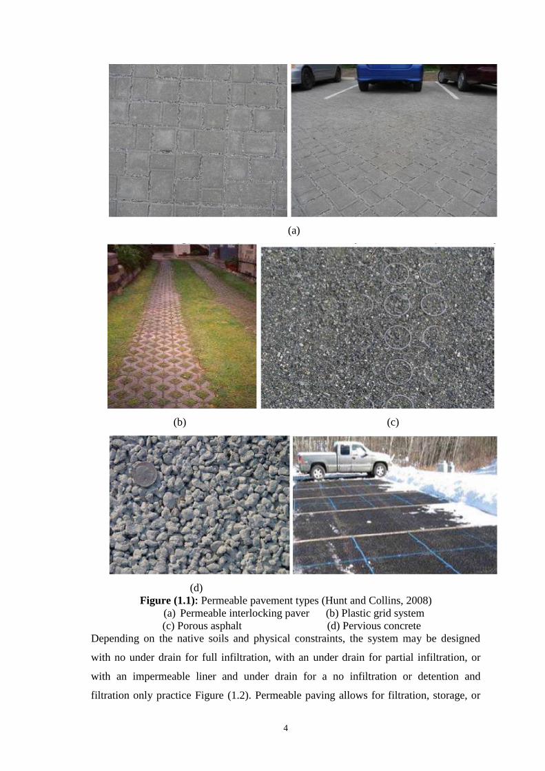
pavement types are illustrated in Figure (1.1):
permeable interlocking concrete pavers (i.e., block pavers);
plastic or concrete grid systems (i.e., grid pavers);
pervious concrete; and
porous asphalt.
4
(a)
(b) (c)
(d)
Figure (1.1): Permeable pavement types (Hunt and Collins, 2008)
(a) Permeable interlocking paver (b) Plastic grid system
(c) Porous asphalt (d) Pervious concrete
Depending on the native soils and physical constraints, the system may be designed
with no under drain for full infiltration, with an under drain for partial infiltration, or
with an impermeable liner and under drain for a no infiltration or detention and
filtration only practice Figure (1.2). Permeable paving allows for filtration, storage, or

5
infiltration of runoff, and can reduce or eliminate surface storm water flows compared
to traditional impervious paving surfaces like concrete and asphalt.
Figure (1.2): Permeable pavement cross sections
(Greater Vancouver Regional District, 2005)

6
1.4 Statement of the problem
The available water resources in the Gaza Strip are limited and do not fulfill the
increasing water demand. The Strip depends mainly on the groundwater from the
coastal aquifer, which has a safe yield of only 98 Mm3 per year (Hamdan 1999), while
the overall water demand was estimated at 180 Mm3 per year in 2018 (PWA, 2018 ).
This leads to an annual water deficit in the water resources of about 70 Mm3, which has
its impact on the supplied water quantities as well as their water quality due to sea water
intrusion and deep groundwater up coning. The average annual rainfall gives a bulk
amount of water of about 114 Mm3 (PWA 2007), from which only 45 Mm3 infiltrate
naturally to the aquifer which forms only 40% of the total rainfall (Hamdan and
Muheisen 2003).
With increased population and climate change water shortage problems are troubling
mankind all over the world. How to harvest the water during rainfall events for use at
times of need is of major interest subject to engineers, environmentalists and to the
community. with urbanization, more impervious road and roof surfaces appear resulting
in increased runoff from rainfall. Also don’t forget that Gaza Strip suffering during
winter seasons from flooding, and photo (1.3) show the situation during heavy rain.
This fact led to search about the useful solution of this problem and to improve of the
quality and the quantity of groundwater and Preserving water sources, and to be more
focus to find the tools for treatment of storm water and recharge it to the groundwater
(Khalaf, 2005). Figure (1.3) shows the bad storm water situation in Gaza strip.
Figure (1.3): The bad storm water situation in the Gaza strip

7
1.5 Research Importance
The following points show the importance of this study:
Finding useful methods to reduce the amount of water accumulated at
roads, that causing damage and contamination of the environment.
This study will be as reference to help researchers and engineers to
understand the porous interlock and perform more studies and researches
in the same field.
Suggesting useful way to collect water and recharging in ground water.
Preservation the existing raw materials and natural resources.
1.6 Research goal and objectives
1.6.1 Goal
The main goal of this research is to study the possibility of producing
and using porous interlock in Gaza strip to avoid disadvantages and
problems in the existed pavement due to some special cases like runoff.
1.6.2 Objectives
To be more specific, this research represents a trial to:
Study the different characteristics and properties of porous interlock.
Evaluate the possibility of producing and using porous interlock in the
Gaza strip.
Studying the properties of the locally available materials that using in
producing porous interlock as aggregate , basalt and cement.
Provide guidance for engineers, contractors, and government
agencies in dealing with permeable pavement as a storm water management
technique in the Gaza strip.

8
1.7 Methodology
In order to achieve the objectives of this study, methodology consists of a theoretical and
a practical study as follows:
1.7.1 Theoretical Study
a. Review of literature, publications, books, journals and data collection about the
permeable pavement and mix design for interlock.
b. Literature review of previous studies which including the same system in other
countries.
c. Study of concrete block types and shapes that available in Gaza and knowing of
its dimensions and characteristics, then study the properties of materials using in
concrete blocks as a fine aggregate.
d. Study on porous interlock and pavement pattern to achieve maximum
permeability of water.
1.7.2 Practical Study
a. Material collection
After carrying out the above study and deciding which approach is suitable for
permeability to make a prototype test, the material needed for producing porous
interlock was collected such as (aggregate, cement, and sand) and filling or beading
materials, data includes information needed for modeling must be used to develop a
rainfall simulator with certain intensity.
b. Experimental study
Here the most focus and concentration were in the laboratory.
During the field work from 15 to 20 samples of porous interlock was prepared in the
automatic factory and then the samples were transport to laboratory and applied to
making test. These samples were prepared to determine:
The best grading system and the best aggregate percentage that should be
used in the porous interlock materials.
Size and shape of porous interlock.
Water cement ratio.
Strength of interlock, density and voids ratio.

9
c. Analysis and results’ discussion
After conducting the practical tests in the laboratory, the results were analyzed
and discussed. It is important it to mention that many figures and tables were
used here to represent and describe the results in order to suggest effective
recommendation.
d. Drawing conclusion and recommendations.
After the completion of the laboratory tests and documentation of the results and
the collection of the results of permeability after the work of simulations of the
intensity rate the final step, conclusion and recommendations .
1.8 Thesis outline
The thesis consists of five chapters that cover the subjects follows:
Chapter (1): Introduction
This chapter is a brief introduction on permeable pavement system ,In addition,
statement of problem, aim, objectives, research contribution, and methodology of
research are described.
Chapter (2): Literature review
This chapter consists of a general introduction with an overview of permeable
pavement, definition and the types of permeable pavements. The advantages of using
permeable pavements such as reducing storm water peak flow rates.
Chapter (3): Experimental Program
This chapter describes the experimental program in laboratory, and testing method. The
infiltration tests carried out on the laboratory pavement and the results of these tests
were presented in this chapter, and describe the scenarios that have been used on study.
Chapter (4): Results and Discussions
The achieved results of laboratory work are illustrated in this chapter, result of
experimental scenarios (compressive strength & absorption) and result of permeability.
Chapter (5) : Conclusions and Recommendations
This chapter presents conclusions and recommendations based on findings from the
Study.

10
Chapter (2)
Literature Review

11
2.1 Introduction
This chapter of thesis considers the theoretical part of study, presents and collects the
information of permeable pavements, the different types of permeable pavements,
Benefits of permeable pavement, Use of permeable pavement, Construction,
maintenance and performance of permeable pavement. The preparation of the layer
under permeable pavement includes material selection for the bedding and base course
The major characteristic of permeable pavements were reviewed and investigated the
traditional concrete block types, some studies were conducted in this concern and the
outcome of these studies was reviewed.
2.2 Overview of Permeable Pavement
Permeable pavements are alternatives to traditional impervious asphalt and concrete
pavements. Interconnected void spaces in the pavement allow for water to infiltrate into
a subsurface storage zone during rainfall events. In areas underlain with highly
permeable soils, the captured water infiltrates into the sub-soil. In areas containing soils
of lower permeability, water can leave the pavement through an under drain system.
2.2.1 Types of Permeable Pavements
There are five types of permeable pavements: permeable asphalt (PA), permeable
concrete (PC), permeable interlocking concrete pavers (PICP), concrete grid pavers
(CGP), and plastic grid pavers (PG). The pictures in Figure (2.1) illustrate the five types
and a variation of fill for plastic grid pavers.
Figure (2.1): Type of permeable pavements (NRMCA, 2004)

12
Permeable concrete (PC)
Is a mixture of Portland cement, fly ash, washed gravel, and water. The water to
cementitious material ratio is typically 0.35 – 0.45. Unlike traditional installations of
concrete, permeable concrete usually contains a void content of 15 to 25 percent,
which allows water to infiltrate directly through the pavement surface to the
subsurface. A fine, washed gravel, less than 13 mm in size (No. 8 or 89 stone), is
added to the concrete mixture to increase the void space. An admixture improves the
bonding and strength of the pavements. These pavements are typically laid with a 10
to 20 cm (4 – 8 in) thickness and may contain a gravel base course for additional
storage or infiltration. Compressive strength can range from 2.8 to 28 MPa (400 to
4,000 psi) (National Ready Mixed Concrete Association, NRMCA, 2004).
Permeable asphalt(PA)
Consists of fine and course aggregate stone bound by a bituminous-based binder.
The amount of fine aggregate is reduced to allow for a larger void space of typically
15 to 20 percent. Thickness of the asphalt depends on the traffic load, but usually
ranges from 7.5 to 18 cm (3 – 7 in). A required underlying base course increases
storage and adds strength (Ferguson, 2005).
Permeable interlocking concrete (PICP)
Pavements are available in many different shapes and sizes. When lain, the blocks
form patterns that create openings through which rainfall can infiltrate. These
openings, generally 8 to 20 percent of the surface area, are typically filled with pea
gravel aggregate, but can also contain top soil and grass. ASTM C936 specifications
(200 1b) state that the pavers be at least 60 mm (2.36 in) thick with a compressive
strength of 55 MPa (8,000 psi) or greater. Typical installations consist of the pavers
and gravel fill, a 38 to 76 mm (1.5 – 3.0 in) fine gravel bedding layer, and a gravel
base-course storage layer (ICPI, 2004).
Concrete grid pavers (CGP)
CGP are typically 90 mm (3.5 in) thick with a maximum 60 × 60 cm (24 × 24 in)
dimension. The percentage of open area ranges from 20 to 50 percent and can
contain topsoil and grass, sand, or aggregate in the void space. The minimum
average compressive strength of CGP can be no less than 35 MPa (5,000 psi). A
typical installation consists of grid pavers with fill media, 25 to 38 mm (1 – 1.5 in)
of bedding sand, gravel base course, and a compacted soil subgrade (ICPI, 2004).
13
Plastic reinforcement grid pavers (PG)
Also called geocells, consist of flexible plastic interlocking units that allow for
infiltration through large gaps filled with gravel or topsoil planted with turf grass. A
sand bedding layer and gravel base-course are often added to increase infiltration
and storage. The empty grids are typically 90 to 98 percent open space, so void
space depends on the fill media (Ferguson, 2005). To date, no uniform standards
exist; however, one product specification defines the typical load-bearing capacity
of empty grids at approximately 13.8 MPa (2,000 psi). This value increases up to 38
MPa (5,500 psi) when filled with various materials.
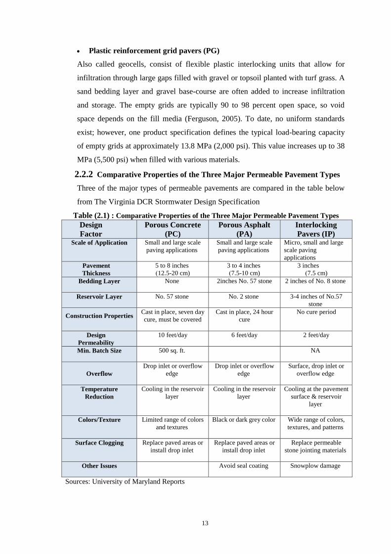
2.2.2 Comparative Properties of the Three Major Permeable Pavement Types
Three of the major types of permeable pavements are compared in the table below
from The Virginia DCR Stormwater Design Specification
Table (2.1) : Comparative Properties of the Three Major Permeable Pavement Types
Design
Factor
Porous Concrete
(PC)
Porous Asphalt
(PA)
Interlocking
Pavers (IP) Scale of Application Small and large scale
paving applications
Small and large scale
paving applications
Micro, small and large
scale paving
applications
Pavement
Thickness
5 to 8 inches
12.5-20 cm))
3 to 4 inches
7.5-10 cm))
3 inches
7.5 cm))
Bedding Layer
None
2inches No. 57 stone 2 inches of No. 8 stone
Reservoir Layer
No. 57 stone
No. 2 stone
3-4 inches of No.57
stone
Construction Properties
Cast in place, seven day
cure, must be covered
Cast in place, 24 hour
cure
No cure period
Design
Permeability
10 feet/day
6 feet/day
2 feet/day
Min. Batch Size
500 sq. ft.
NA
Overflow
Drop inlet or overflow
edge
Drop inlet or overflow
edge
Surface, drop inlet or
overflow edge
Temperature
Reduction
Cooling in the reservoir
layer
Cooling in the reservoir
layer
Cooling at the pavement
surface & reservoir
layer
Colors/Texture
Limited range of colors
and textures
Black or dark grey color
Wide range of colors,
textures, and patterns
gingSurface Clog
Replace paved areas or
install drop inlet
Replace paved areas or
install drop inlet
Replace permeable
stone jointing materials
Other Issues
Avoid seal coating
Snowplow damage
Sources: University of Maryland Reports

14
2.3 Permeable Interlocking Concrete Pavement (PICP)
Permeable interlocking concrete pavement, also referred to as PICP, consists solid
concrete paving units with joints that create openings in the pavement surface when
assembled into a pattern. The joints are filled with permeable aggregates that allow
water to freely enter the surface. The permeable surface allows flow rates as high as
(2,540 cm/hr). The paving units are placed on a bedding layer of permeable aggregates
which rests over a base and subbase of open-graded aggregates. The concrete pavers,
bedding and base layers are typically restrained by a concrete curb in vehicular
applications. The base and subbase store water and allow it to infiltrate into the soil
subgrade. Perforated underdrains in the base or subbase are used to remove water that
does not infiltrate within a given design period, typically 48 to 72 hours. Geo synthetics
such as geotextiles, geogrids or geomembranes are applied to the subgrade depending
on structural and hydrologic design objectives. Separation geotextiles are used on the
sides of the base/subbase to prevent entrance of fines from adjacent soils(Borst, 2010).
2.3.1 History of (PICP)
Road paving with tightly fitted stones resting on a flexible granular base dates back to
the Roman Empire. Even though, stones are still being used as paving material the
modern version of this road technique utilizes concrete blocks instead. [Rada et. al.
1990]. The use of concrete block pavement CBP for roads began in the Netherlands
after the Second World War. Brick paving was the traditional surface material in the
Netherlands before the Second World War. Because of the coal shortages brick had
been unavailable as a result CBP had been used as a substitute. The substitution became
hugely successful. After the war, the roads of Rotterdam were almost entirely
constructed from concrete block paving [Pritchard and Dawson 1999]. This technology
quickly spread to Germany and Western Europe as a practical and attractive method
useful for both pedestrian and vehicular pavement [Rada et. al. 1990]. Over the past 40
years CBP has gained rapid popularity as an alternative to conventional concrete and
asphalt pavements. The CBP is now a standard paving surface in Europe where over
100,000,000 m2 are placed annually [Ghafoori and Mathis 1998].
In Australia
Interlocking concrete blocks were introduced into Australia in 1976. By 1979 sales
figures had reached 2 km2 per annum and are currently increasing rapidly. Until
recently, very little scientific investigation had been carried out into the performance of

15
block paving under traffic and the design and construction of block pavements had been
based on European experience or modifications of flexible pavement design procedures.
The first full-scale testing of block pavements of any significance in Australia began in
1977 at the University of New South Wales test track.
2.3.2 Typical permeable interlocking concrete pavement cross section.
Figure (2.2) illustrates PICP components. The figure shows a partial infiltration design
with drainage to accommodate some water that does on enter low infiltration soils.
PICP over high infiltration subgrade soils may not require an underdrain(s) and these
are called are called full infiltration designs. Other designs over expansive or fill soils or
close to buildings may enclose the pavement structure with geomembrane (impermeable
liner). An outlet pipe provides temporary storage and outflow control. This design
approach also can be used for water harvesting or for horizontal ground source heat
pumps. The use of a geomembrane to restrict infiltration into the soil subgrade is often
called a no infiltration design.
Figure (2.2): PICP components (PICP Institute)
2.3.3 Requirements of (PICP)

16
PICP may help achieve compliance with many national, provincial, state and local
regulations as well as transportation agency design requirements for stormwater runoff
control. These requirements may include the following:
Limits on impervious cover (i.e., roofs and pavements) and resulting runoff .
Runoff volume storage and/or infiltration to reduce overflows, especially
combined sewer overflows.
Meeting total maximum daily load (TMDL) requirements for receiving waters.
Managing water quality volume capture and or quantity storm events.
2.4 Concrete block pavement (CBP)
Pavements have been surfaced with stone blocks since ancient times and even up to the
end of the 19th century surfaces of dressed stone or hardwood blocks were common.
Developments in concrete technology and improved plant for block manufacture led to
acceptance of small concrete blocks for pavement surfaces in Western Europe about 60
years ago(CCA, 1988).
2.4.1 Features of Concrete Block Pavements Concrete paving blocks are utilized in a variety of commercial, municipal and industrial
applications. The primary reasons for selecting CBP over other paving surfaces are low
maintenance, ease of placement and removal, reusage of original blocks, aesthetics
appeal, and immediate usage after installation or repair [Ghafoori and Mathis 1998].
CBPs are able to withstand heavy loads and resists aggressive environments as good as
a rigid concrete pavement. Besides that, with its wide range of colors, textures and
patterns, CBPs provide excellent aesthetic appearance opportunities.
Aesthetic Appeal
Concrete block paving is available in a constantly expanding variety of colors, shapes
and textures and can be installed in numerous bonds and laying patterns [Interpave
2003]. Concrete pavers offer unique aesthetic benefits when compared to other forms of
pavement in their ability to integrate and harmonize with both the built and natural
environment [Concrete Masonry Association of Australia 1997]. In Figure (2.3) some
applications of paving blocks are provided.
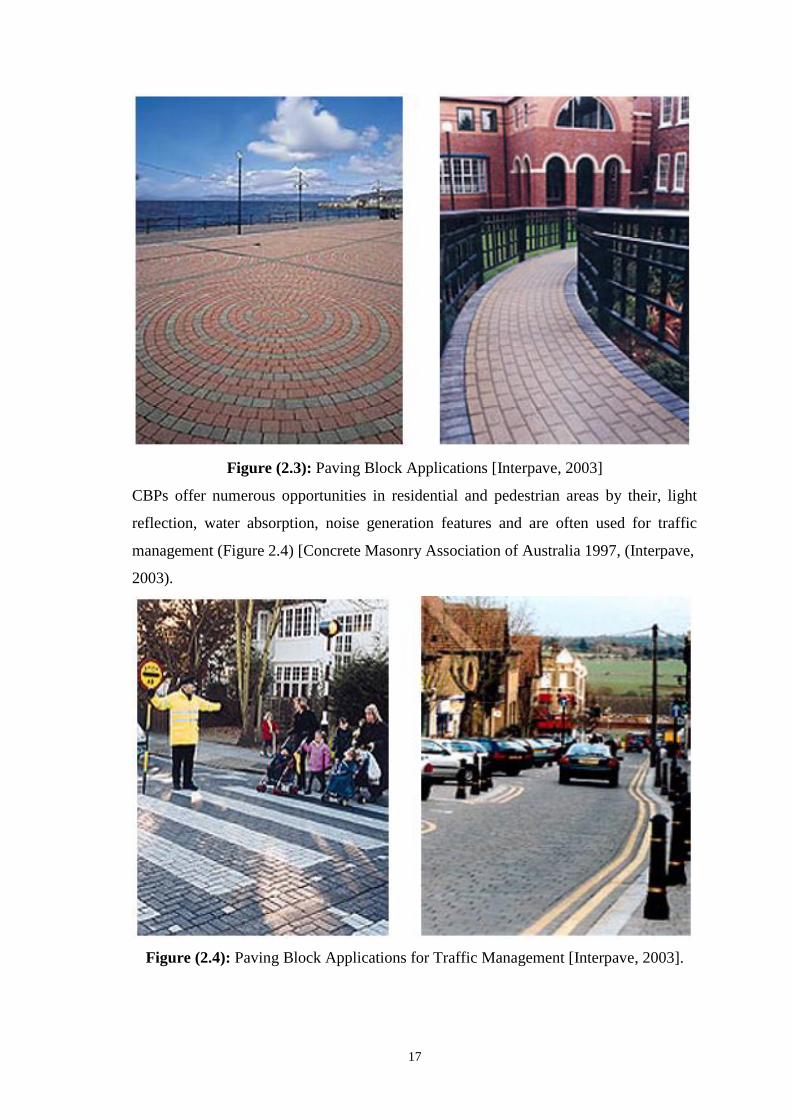
17
Figure (2.3): Paving Block Applications [Interpave, 2003]
CBPs offer numerous opportunities in residential and pedestrian areas by their, light
reflection, water absorption, noise generation features and are often used for traffic
management (Figure 2.4) [Concrete Masonry Association of Australia 1997, (Interpave,
2003).
Figure (2.4): Paving Block Applications for Traffic Management [Interpave, 2003].

18
2.4.2 Applications of concrete block pavement
Concrete pavers are a versatile paving material, which due to the availability of many
shapes, sizes and colors, have endless streetscape design possibilities. The use of
concrete block paving can be divided into the following categories:
Roads:
Main roads, residential roads, urban renewal, intersections, toll plazas, pedestrian
crossings, taxi ranks, steep slopes, pavements (sidewalks), and figure (2.5) show
example of road application.
Figure (2.5): Example of Roads Applications
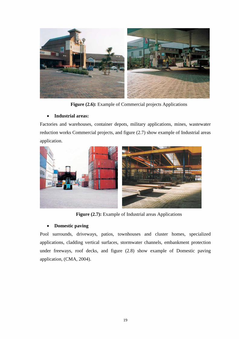
Commercial projects:
Car parks, shopping centers and malls, parks and recreation centers, golf courses and
country clubs, zoos, office parks, service stations, bus termini, and figure (2.6) show
example of Commercial projects application.
19
Figure (2.6): Example of Commercial projects Applications
Industrial areas:
Factories and warehouses, container depots, military applications, mines, wastewater
reduction works Commercial projects, and figure (2.7) show example of Industrial areas
application.
Figure (2.7): Example of Industrial areas Applications
Domestic paving
Pool surrounds, driveways, patios, townhouses and cluster homes, specialized
applications, cladding vertical surfaces, stormwater channels, embankment protection
under freeways, roof decks, and figure (2.8) show example of Domestic paving
application, (CMA, 2004).

20
Figure (2.8): Example of Domestic paving Applications
Specialized Applications Cladding vertical surfaces, Stormwater channels, Embankment protection under
freeways, Roof decks, and figure (2.9) show example of Specialized application, .
Figure (2.9): Example of Specialized Applications
2.4.3 Pattern in Concrete Block Pavements
Concrete block pavements are produced in a variety of shapes, typical paving block
shapes available in the Gaza strip are shown in Figure (2.10).
Concrete block pavers come in a variety of shapes and sizes.
If we consider for a moment the aesthetics of concrete block paving, three fundamental
aspects present themselves:
Shapes
The illustration below Figure (2.10) shows the range of available shapes and trade
names in Gaza strip.

21
Figure (2.10):Available Block shapes in the Gaza strip
(Available in Mushtaha & Hassouna Company)
Colors
Illustrated below Figure (2.11) are some of the range of standard colors available. Many
pigments are used by paving block manufacturers which, together with aggregates from

22
different areas and various cements, produce a huge variety of colors from which to
choose. Multiblends are produced by the incomplete mixing of pigments and give a
pleasing effect when laid over large areas.
Figure (2.11):Available Colors of Block Pavement
Patterns
Laying patterns of pavers are identified as being either herringbone, basket weave,
or stretcher as shown below. Each of these may be laid at either 90o or 45o to the
line of edge restraints. A variation of stretcher is the Zig zag running bond (CMA,
2004). Figure (2.12),shows the pavement pattern.
Figure (2.12) : Pavement Patterns (CMA, 2004)
2.4.4 Characteristics of concrete block pavements in the Gaza Strip
Palestine Standards Institution (PSI)shows the characteristics and specifications as:
The compressive strength of concrete block should be between 45 and 50 MPa.
The value of the Abrasion value rate should be no more than 5-6 mm.
The Maximum absorption when placed in water for 10 minutes no more than 2%
and when placed in water for 24 hour no more than 5%.
Pav
emen
t P
atte
rn
Herringbone bond
(90o) Stretcher bond (45o)
Basket weave
bond Zig zag running bond

23
2.4.5 Installation of concrete block pavements
This pavement structure is commonly used for both pedestrian and vehicular
applications. Pedestrian areas, driveways, and areas subject to limited vehicular use
are paved with (60 mm) thick. Streets and industrial pavements should be paved
with units at least (80 mm) thick.
Figure from (2.13) to(2.17) ,shows the installation steps.
Figure (2.13) :Excavation and compacting of the soil subgrade
Figure (2.14) : Base compaction with a vibratory roller Figure (2.15) : Screeding the bedding sand

24
Figure (2.16) : Placing the concrete pavers Figure (2.17) : Compacting the pavers and bedding sand
2.5 Porous pavements (P.P)
Porous pavements are those made with built-in void spaces that let water and air pass
through. They are the most radical, most rapidly developing, and most controversial
way of restoring large parts of the urban environment. They have been called “the holy
grail of environmental site design” and “potentially the most important development in
urban watersheds since the invention of the automobile (Schaus, 2007).
In the late 1960’s, research into a new type of pavement structure was commencing at
The Franklin Institute Research Laboratories (FIRL) in the United States. With the
support of the United States Environmental Protection Agency (EPA), a porous
pavement program was developed. This new pavement structure was initially installed
in parking lots (Schaus, 2007).
Porous pavements have been installed since the early 1980’s throughout the United
States, installed over on parking lots, pathways, and trails for universities, libraries,
religious centers, prisons, industrial parks, commercial plazas, and municipal
buildings(Adams, 2006).
The original proposed structure of a porous pavement consisted of an open graded
surface course placed over a filter course and an open graded base course (or reservoir)
all constructed on a permeable subgrade. Stormwater infiltrations using pervious
pavements have been investigated by researchers as a method of managing storm water
(Schaus, 2007).

25
2.5.1 Porous concrete’s environmental performance
Properly installed porous concrete has void space of 11 to 22 percent (the amount varies
with aggregate type). Its surface infiltration rate is over 55 inches per hour, and can
exceed 100 inches per hour.
Like other porous paving materials, porous concrete reduces stormwater rate and
volume. Stormwater can be discharged through a perforated pipe at the bottom of the
pavement, or at the top of the base reservoir, or water can be allowed to overflow at the
pavement surface. Each type of drainage outlet produces different proportions of
detention, treatment, infiltration, evaporation, and lateral overflow. Rainwater
infiltration through a porous pavement into the underlying soil reduces stormwater
volume and restores natural subsurface flow paths. Where slowly permeable soil
prohibits significant soil infiltration, and water is discharged through a perforated pipe
in the pavement, a porous pavement can perform detention comparable to that in off-
pavement reservoirs and ponds: the peak discharge of stormwater from the bottom of a
porous pavement is later and lower than that of the rainfall entering it at the top; the
total volume of discharge is lower. Reduction of stormwater flow reduces downstream
flood frequency, stream channel erosion, sediment loads, and combined-sewer
overflows.
It is believed that common urban pollutants are treated in porous concrete, as they are in
other types of porous pavement. Metals like cadmium and lead released by automobile
corrosion and wear are captured in porous pavements’ voids along with the minute
sediment particles to which the ions are characteristically attached. Capturing then
metals prevents them from washing downstream and accumulating inadvertently in the
environment. In the void spaces, oil leaked from automobiles is digested by naturally
occurring micro biota that inhabit the abundant internal surface area. The oil’s
constituents go off as carbon dioxide and water, and very little else; the oil ceases to
exist as a pollutant.
Porous pavements combine stormwater management with pavement function in a single
structure. Developments planned to benefit from this combination tend to cost less than
those having impervious pavements with separate stormwater management facilities
that incur costs of land acquisition, excavation, piping, and outlet structures.
Porous pavements can give urban trees the rooting space they need to grow to full size,
providing the shade, cooling and air quality for which the trees are planted. The rooting
zone is an aggregate base, made of large, single-sized aggregate that bears the

26
pavement’s load. Into the aggregate’s void space is mixed 15 to 20 percent by volume
of nutrient- and water-holding soil; the remaining unfilled void space maintains aeration
and drainage. The base mixture makes the base into a “structural soil”, while the porous
surface admits vital air and water to the rooting zone. This is a revolutionary new way
to integrate healthy ecology and thriving cities: living tree canopy above, the city’s
traffic on the ground, and living tree roots below.
2.5.2 Porous concrete’s potential
Porous pavements are important because they can solve urban environmental problems
at the source. In new suburban growth, they protect pristine watersheds. In old town
centers, redevelopment and reconstruction are opportunities for environmental
rehabilitation simultaneously with urban renewal.
The hydrologic and structural success of porous concrete depends on correct selection,
design, installation, and maintenance. Failures — clogging and structural degradation
— result from neglecting one or more of these steps. Porous pavements’ potential
application is vast. To date, porous pavements constitute only a minute fraction of the
paving done each year in the United States. But their rate of growth, on a percentage
basis, is very high, primarily because of public concern about and legal requirements for
stormwater management. Properly applied porous pavements can also enlarge urban
tree rooting space, reduce the urban heat-island effect, reduce traffic noise, increase
driving safety, and improve appearance. Therefore their selection and implementation
are integral parts of the multi-faceted concerns of urban design, and all of their effects
are considered together in evaluations of potential benefits and costs.
2.6 Drainage design for permeable pavement
Drainage design is only one important part of the integrated pervious pavement system.
According to different drainage designs underneath the pervious surface, pervious
pavements can achieve objectives when used as a stormwater management method.
Normally the designed flows will be estimated by the Rational Method, as show in eq.
(2.1).
Q = C I A---------------------------------------- (2.1)
Where,
Q = Storm water quantity, (m3/h)
C = Coefficient of Runoff, (dimensionless)
I = Rainfall intensity, (mm/h)
A = Catchment Area, (m2)

27
According to the local environmental and stormwater resource requirements, different
drainage pipe designs can be integrated into the pervious pavement systems at design.
For example, if the local groundwater table is at a significant low depth, stormwater is
an ideal resource to recharge groundwater. Under this situation, the aim of the pervious
pavement is to allow more water to percolate into the groundwater bringing it up ready
for reuse. In this situation the drainage pipe is laid close to the bottom of bedding layer.
2.7 Storm water data in Gaza
The necessary information required by the research have been collected from the
relevant institutions such as Palestinian water authority (PWA), municipalities, the
Ministry of Local Government (MOLG), the Ministry of Agriculture (MOA), Coastal
municipal water utility (CMWU) and local NGOs.
The available stormwater quantities that flow from the existing urban areas in Gaza
were calculated to be 22 Mm3 every year. Since urbanization in the Gaza Strip is a
continuous process, the flowing stormwater quantities from the planned land use were
estimated to be 37 Mm3 every year (Hamdan, and Nassar, 2007).
The available groundwater system which is part of the coastal aquifer showed fast
response to natural rainfall infiltration. However, in the dry season, the decrease in the
water table was around 1.5 meters due to groundwater abstraction. This means that the
supply to the aquifer is much less than the demand through abstraction. At the same
times, there it gives us an indication that, artificial recharge of groundwater with
stormwater will have quick positive effect to balance the gap between aquifer supply
and demand (Hamdan, and Nassar, A., 2007).
2.7.1 Rain Intensity
Improvement of the reliability of Rain Intensity (RI) measurements as obtained by
traditional tipping-bucket rain gauges and other types of gauges (optical, weighting,
floating/siphoning, etc.) is therefore required for use in climatologic and hydrological
studies and operationally e.g. in flood frequency analysis for engineering design.
Standardization of high quality rainfall measurements is also required to provide a basis
for the exchange and valuation of rainfall data sets among different countries, especially
in case transboundary problems such as severe weather/flood forecasting, river
management and water quality control are operationally involved. Figure(2.18) shows
the intensity duration frequency curve in Gaza city, where the intensity readings taken

28
from curves of return period.
Figure (2.18): Rainfall Intensity/Duration Meteorological Recording Station (unrwa, 1980)
2.8 Permeable paving advantage and risk
2.8.1 Advantages of concrete block pavements
Two of the major advantages of concrete block pavements are their aesthetic appeal and
their high strength. In addition the riding surface of good quality concrete offers high
durability, skid resistance, abrasion and scuffing resistance.
Block pavements may be opened to traffic immediately on completion of construction,
the surface is not as smooth as asphalt or cast in situ concrete so interlocking pavements
are generally recommended for where traffic speeds are less than 50-60 km/h. Because
of its segmental nature, interlocking blocks can be recycled. Once the pavement has
been broken, paving blocks can be lifted and recovered for re-use and only a small stock
of replacement blocks needs to be maintained. This facilitates access to underground
services and permits the subsequent restoration of the pavement with little material cost
and no discontinuity of the surface. Pavement shape correction if required can also be
accomplished at low material cost (CCA, 1988).
2.8.2 Permeable paving risk
Common concerns about permeable paving include the following:
Risk of Groundwater Contamination:
Most pollutants in urban runoff are well retained by infiltration practices and soils and
therefore, have a low to moderate potential for groundwater contamination (Pitt et al.,
1999). Chloride and sodium from de-icing salts applied to roads and parking areas

29
during winter are not well attenuated in soil and can easily travel to shallow
groundwater. Infiltration of deicing salt constituents is also known to increase the
mobility of certain heavy metals in soil .
Risk of Soil Contamination:
Available evidence from monitoring studies indicates that small distributed stormwater
infiltration practices do not contaminate underlying soils, even after more than 10 years
of operation (TRCA, 2008).
Winter Operation:
For cold climates, well-designed mixes can meet strength, permeability, and freeze-
thaw resistance requirements. In addition, experience suggests that snow melts faster on
a porous surface because of rapid drainage below the snow surface. Also, a well-
draining surface will reduce the occurrence of black ice or frozen puddles (Cahill
Associates, 1993, Roseen, 2007). Permeable pavement is typically designed to drain
within 48 hours. If freezing should occur before the pavement structure has drained,
then the large void spaces in the open graded aggregate base creates a capillary barrier
to freeze-thaw. Permeable pavers have the added benefit of having enough flexibility to
handle minor heaving without being damaged. Permeable pavement can be plowed,
although raising the blade height 25 mm
may be helpful to avoid catching pavers or scraping the rough surface of the porous
pavement. Sand should not be applied for winter traction on permeable pavement as this
can quickly clog the system(TRCA, 2008).
On Private Property:
If permeable pavement systems are installed on private lots, property owners or
managers will need to be educated on their routine maintenance needs, understand the
long-term maintenance plan, and may be subject to a legally binding maintenance
agreement. An incentive program such as a storm sewer user fee based on the area of
impervious cover on a property that is directly connected to a storm sewer . could be
used to encourage property owners or managers to maintain existing practices.
30
Clogging:
Susceptibility to clogging is the main concern for permeable paving systems. The
bedding layer and joint filler should consist of 2.5 mm clear stone or gravel rather than
sand. Key strategies to prevent clogging are to ensure that adjacent pervious areas have
adequate vegetation cover and a winter maintenance plan that does not include sanding.
For concrete and asphalt designs, regular maintenance that includes vacuum-assisted
street sweeping is necessary. Isolated areas of clogging can be remedied by drilling
small holes in the pavement or by replacing the media between permeable pavers.
Road Salt:
Care needs to be taken when applying road salt to permeable pavement surfaces since
dissolved constituents from the road salt will migrate through the bedding and into the
groundwater system. A well-draining surface will reduce the occurrence of black ice or
frozen puddles and requires less salt than is applied to impervious pavement (Roseen,
2007).
Structural Stability:
Adherence to design guidelines for pavement design and base coarses will ensure
structural stability. In most cases, the depth of aggregate material required for the
stormwater storage reservoir will exceed the depth necessary for structural stability.
Reinforcing grids can be installed in the bedding for applications that will be subject to
very heavy loads.
Heavy Vehicle Traffic:
Permeable pavement is not typically used in locations subject to heavy loads. Some
permeable pavers are designed for heavy loads and have been used in commercial port
loading and storage areas.
2.9 Maintenance of (PICP):
Openings in the surface of permeable pavements are susceptible to clogging by
sediment from passing vehicles, wear of the pavement surface, and runoff from nearby
disturbed soils. It is therefore essential to ensure that nearby soils are adequately
secured prior to, during, and after installation of permeable pavement.
Pretreatment systems may be required to help prevent clogging. Legally binding
easements or covenants may be needed to ensure proper maintenance techniques are
followed.

31
Maintenance should be performed on a regular basis. To prevent clogging, the
permeable pavement surface should be vacuum swept followed by high-pressure jet
hosing at least four times per year. Do not apply sand or ash to permeable pavement
for snow removal purposes. Signage should be posted at locations where permeable
pavement is installed to advise maintenance crews of this requirement.
Routine Maintenance
The following provides a checklist for PICP routine maintenance:
Inspect, and if necessary, clean the surface using regenerative air equipment to
remove debris and sediment in the spring and late fall.
Repair/replant vegetative cover for areas up slope from the PICP
Replenish aggregate in joints if more than ½ in. (13 mm) from paver chamfer
bottoms
Repair all paver surface deformations exceeding ½ in. (13 mm)
Repair pavers offset by more than ¼ in. (6 mm) above/below adjacent units or
curbs, inlets etc.
Replace cracked paver units impairing surface structural integrity
Clean and flush underdrain system if slow draining
Clean drainage outfall features to ensure free flow of water and outflow
Remedial Maintenance
Repair and/or reinstatement of damaged edge restraints and resulting movement
in the pavers; this may require removal and reinstatement of adjacent paving
units
Repair localized settlement greater than ½ in. (13 mm) and rutted pavement
areas
Repair outflow features, piping, energy dissipaters, erosion protection systems,
etc. as required
Winter Maintenance
Avoid the use of winter sand for traction; if used, remove with regenerative air cleaning
equipment in the spring (regenerative equipment does not evacuate jointing materials)
Remove snow with standard plow/snow blowing equipment
Stockpile plowed snow onto turf or other vegetated areas and not on the PICP.

32
Monitor temperatures and apply anti-icing/deicing materials such as sodium
chloride, calcium chloride or magnesium calcium acetate.
2.10 Conclusion of previous studies
After reviewing the previous studies and during researching to complete the thesis, we
were review a lot of studies related to porous/permeable/pervious pavements with
respect to interlocking concrete pavers, all of these pavements are designed to allow
free draining through the structure. The local studies is more less than international
studies ,and these studies as follow:
In Gaza
Eng. Mahmoud Madhoun with supervision of Prof. Shafiq Jendia present study " the
Effect of Joints, Block Shape and Pavement Pattern on the Permeability of Concrete
Block Pavement (Interlock Pavement).The conclusion of the study was:
The results show that the using rectangular block tile 10x20 cm gives the
highest percentage of water permeability.
The increase of joints between interlock tiles, no large effect has been noticed in
the percentage of water permeability during low intensity of water, while little
increase was observed in the water permeability during the high water intensity
but the increase in the continuity of water permeability grows with the increase
of joints in cases of obstructive dust and dirt on the surface of the pavement.
In world
Study by (H.M. Imran, Shatirah Akib and Mohamed Rehan Karim), University of
Malaya, Kuala Lumpur, Malaysia (3 March 2013), on " Permeable pavement and
stormwater management systems" The conclusion of the study was:
Permeable pavement system PPS play a vital role in reducing contaminants from
infiltrating stormwater runoff and provide great facilities for storage and the
reuse of stormwater as well
as in preserving the hydrologic function of a site.
PPS can be applied to reduce the increased pressure on groundwater extraction.
permeable pavement technology, is a green approach to collecting, storing,
treating and reusing stormwater from residential, industrial commercial areas.
Study by (Mulian Zheng,Shuanfa Chen, and Binggang Wang) Mar 2012 on " mix
design method for permeable base of porous concrete " describe that:

33
Porous concrete should have certain porosity to fully drain water and in addition
to particular structural strength.
Percentage of porosity range from 30-35 % .
The test was designed with consideration of three factors cement dosage ,water
cement ratio ,and aggregate gradation .

34
Chapter (3)
Experimental Program

35
3.1 Introduction
An update of what was presented in the first and second chapters and a confirmation of
the objectives that have been indicated that the use of permeable pavements to manage
storm water. It is clear that to achieve an efficient and durable solution, a careful design
of pavement layers and choice of surface pavement product. The objective of the
present study is to understand the infiltration through interlock pavement surface only.
In order to reach the goals of the letter we making a number of concrete mixtures and
manufacturing of permeable Interlock using different aggregate type, cement and water
and then do all the necessary tests in the laboratory. The second part, it was decided to build a practical experiment pavement to monitor the
infiltration rates through the pavement structure. The simulated rainfall events were
modeled using the small pipe and nozzles on steel box. The water infiltrated through the
pavement collected by funnel.
Processing of the mixes and collecting of material were at the automatically factory in
Gaza.
Firstly, this chapter presents the laboratory studies carried out to determine the
parameters necessary to build the pavement and to monitor the infiltration rate.
Secondly, to describe how experimental work has been done and the possible scenarios
to achieve study objectives.
3.2 Processing of samples and laboratory testing
This study depends on laboratory testing as the main procedure to achieve study goals,
and the test were conducted using equipment and devices available in the laboratories of
Association of Engineers-Gaza to evaluate the properties of aggregate material and
sand. The sieve analysis is carried out for each aggregate type to obtain the grading of
aggregate sizes.
Laboratory tests are divided into three stages:
1st Stage of Testing
This stage includes the collection of materials for the processing of permeable Interlock
samples, such as types of gravel, sand and cement, then the samples are processed in the
factory in order to control the quality, mixing characteristics and manufacturing
specifications.

36
2nd Stage of Testing
This stage were in the laboratory and includes the work of the necessary tests for the
materials used in the processing of Interlock samples and also conduct tests on the
samples Interlock.
3rd Stage of Testing
At this stage a design were developed to calculate the permeability of the samples that
have been processed, The design of experiment was constructed in a 1.0x1.0m with
0.25m depth from steel box. and Figure (3.1) Flow chart displays the laboratory testing
procedure as the three stages.
Figure ( 0.1) : Flow chart of laboratory testing procedure
Data
Material collection
Material evaluation
Aggregate Sand
Production of sampels
Infiltration system
Analyses and result
Cement

37
3.3 Material selection
Materials required for this study were collected from local factory in the Gaza strip,
such as coarse aggregates, sand, and cement. Table (3.1) shows main and local sources
of these materials.
Table (3.1): Main and local sources of used materials
Source Material
Local Main
Mushtaha &Hassouna
Trading co. and General
Contracting
Lahab (Occupied land) Coarse Aggregates
(Folia,Adasea,Semsemia)
Automatic Factory Local sand (Gaza) Fine Aggregates
(Sand)
Automatic Factory Sanad company,(West Bank) Cements
Figure (3.2): Source of Aggregate (Mushtaha &Hassouna Trading co)
3.4 Material properties
In order to obtain the necessary information to construct permeable interlock, laboratory
tests were carried out to determine the selected aggregate properties.
3.4.1 Aggregates properties
The aggregates commonly used for construct interlock is semsemia. But to construct
permeable interlock can used Semesmia, Adsia, and Folia as shown in Table (3.2),
gradation tests were conducted to determine the size distribution for each aggregate

38
type. (Test on Appendix B)
Table (3.2):Used aggregates types
Particle size(mm) Type of aggregate
0/19.0 Folia
Coarse Aggregates 0/12.5 Adasia
0/9.50 Simsimia
0/0.6 Sand Fine Aggregates
3.4.2 Physical properties of aggregates
In order to define the properties of used aggregates, number of laboratory tests were
conducted, these tests include:
Sieve analysis (ASTM C 136).
Specific gravity test (ASTM C127).
Water absorption (ASTM C128).
Table (3.3) to Table (3.5) presents the aggregate tests results, and note that the results of
aggregate material don’t expresses what happens in the result of concrete mix because
the source of aggregate was not the same.
Table (3.3): Specific Gravity of Aggregates
Simsimia Adasia Folia Properties
1598.0 2968.0 2880.0 g S.S.D Weight
970.6 1808.3 1745.8 g Weight in Water
627.4 1159.7 1134.2 cm3 Volume of Solids
2.547 2.559 2.539 g/cm3 Specific Gravity
2.458 2.504 2.481 g/cm3 Dry Specific Gravity
Table (3.4): Water Absorption of Aggregates
Simsimia Adasia Folia Properties
1598.0 2968.0 2880.0 g S.S.D Weight
1544 2905 2815.5 g Oven Dry Weight
3.5 2.2 2.3 % Water Absorption

39
Table (3.5): Specific Gravity of Sand
Fine Properties
481.4 g Dry Weight
1070.7 g Pycnometer + water
1364.8 g Pycnometer + water +Sample
2.622 g/cm3 Specific Gravity
3.4.3 Sieve analysis of aggregates
According to specification (ASTM C136), aggregates sieve analysis that performed on a
sample of used aggregate for each type of aggregate in a laboratory as shown in Table
(3.6) to Table (3.9).
Table (3.6): Folia Aggregate Sieve Analysis
Dry weight of sample before sieving = 2154g % Passing Cumulative
% Retained
%
Retained
Weight
Retained (gm)
Sieve Opening
Size (mm)
Sieve No.
100.00 0.0 0.00 0.0 25.00 1"
94.73 5.3 5.27 113.5 19.00 3/4"
9.4 90.6 85.33 1838.0 12.50 1/2"
3.9 96.1 5.5 118.5 9.50 3/8"
2.53 97.5 1.37 29.5 4.75 #4
2.53 97.5 0.00 0.0 2.36 #8
2.53 97.5 0.00 0.0 1.18 #16
2.53 97.5 0.00 0.0 0.60 #30
2.53 97.5 0.00 0.0 0.30 #50
2.53 97.5 0.00 0.0 0.15 #100
2.53 97.5 0.00 0.0 0.075 #200
0.0 100.0 2.53 54.5 0.00 Pan
Figure (3.3): Gradation Curve –(Folia 0/19mm)
0.00
10.00
20.00
30.00
40.00
50.00
60.00
70.00
80.00
90.00
100.00
0.01 0.10 1.00 10.00 100.00
% P
assin
g
Sieve Size (mm)

40
Table (3.7): Adsia Aggregate Sieve Analysis
Dry weight of sample before sieving = 2154g % Passing Cumulative
% Retained
%
Retained
Weight
Retained (g)
Sieve Opening
Size (mm)
Sieve No.
100 0 0.00 0.0 25.00 1"
100 0 0.0 0.0 19.00 3/4"
68.75 31.3 31.25 830 12.50 1/2"
19.94 80.1 48.81 1296.5 9.50 3/8"
0.36 99.6 19.58 520.0 4.75 #4
0.26 99.7 0.09 2.5 2.36 #8
0.13 99.9 0.13 3.5 1.18 #16
0.06 99.9 0.08 2.0 0.60 #30
0 100 0.06 1.5 0.30 #50
0 100 0.00 0.0 0.15 #100
0 100 0.00 0.0 0.075 #200
0 100 0.00 0.0 0.00 pan
Figure (3.4): Gradation Curve –(Adasia 0/12.5mm)
0.00
10.00
20.00
30.00
40.00
50.00
60.00
70.00
80.00
90.00
100.00
0.10 1.00 10.00 100.00
% P
assin
g
Sieve Size (mm)

41
Table (3.8): Semsemia Aggregate Sieve Analysis
Dry weight of sample before sieving = 2076g % Passing Cumulative
% Retained
%
Retained
Weight
Retained (g)
Sieve Opening
Size (mm)
Sieve No.
100 0 0.0 0.0 25.00 1"
100 0 0.0 0.0 19.00 3/4"
100 0 0 0.0 12.50 1/2"
98.34 1.7 1.66 34.5 9.50 3/8"
22.28 77.7 76.06 1579.0 4.75 #4
5.06 94.9 17.22 357.5 2.36 #8
2.22 97.8 2.84 59.0 1.18 #16
1.32 98.7 0.89 18.5 0.60 #30
1.08 98.9 0.24 5.0 0.30 #50
0.96 99 0.12 2.5 0.15 #100
0.94 99.1 0.02 0.5 0.075 #200
0 100 0.94 19.5 0.00 pan
Figure (3.5): Gradation Curve –(Semsemia 0/9.5mm)
0.00
10.00
20.00
30.00
40.00
50.00
60.00
70.00
80.00
90.00
100.00
0.10 1.00 10.00 100.00
% P
assin
g
Sieve Size (mm)

42
Table (3.9): Sand Sieve Analysis
Dry weight of sample before sieving = 1945g % Passing Cumulative
% Retained
%
Retained
Weight
Retained (g)
Sieve Opening
Size (mm)
Sieve No.
100 0 0 0.0 25.00 1"
100 0 0 0.0 19.00 3/4"
100 0 0 0.0 12.50 1/2"
100 0 0 0.0 9.50 3/8"
100 0 0 0.0 4.75 #4
100 0 0 0.0 2.36 #8
99.9 0.1 0.1 1.9 1.18 #16
99.6 0.4 0.3 5.86 0.60 #30
93.7 6.3 5.9 115.3 0.30 #50
2 98 91.7 1791.8 0.15 #100
0.2 99.8 1.8 35.2 0.075 #200
0 100 0.2 3.9 0.00 pan
Figure (3.6): Gradation Curve –(Sand 0/0.6mm)
0.0
10.0
20.0
30.0
40.0
50.0
60.0
70.0
80.0
90.0
100.0
0.01 0.10 1.00 10.00 100.00
Sam
ple
Pas
sin
g %
Sieve size (mm)

43
3.5 Production of porous interlock mix
After identifying the properties of the materials that were used in the processing of mix
and supplementing the above, we were review in this part of the research the processing
of samples of porous interlock to conduct the necessary tests for those samples
3.5.1 Number of required samples
To reach the objective of the research, four basic mixtures and with a change in the
quantities of cement and water, the number of samples were reach sixteen samples.
Total number of samples required = approximately 16 samples
Figure(3.7) : show the number of aggregate mix
Figure (3.7): Flowchart of Aggregate Mix Numbers
Agg mix
Aggmix1
mix 1-1 w/c Ratio=0.33
mix 1-2 w/c Ratio =0.36
mix 1-3 w/c Ratio =0.39
mix 1-4 w/c Ratio=0.42
Aggmix2
mix 2-1 w/c Ratio =0.36
mix 2-2 w/c Ratio =0.33
mix 2-3 w/c Ratio =0.42
mix 2-4 w/c Ratio =0.39
Agg mix 3
mix 3-1 w/cRatio =0.39
mix 3-2 w/c Ratio=0.42
mix 3-3 w/c Ratio=0.33
mix 3-4 w/c Ratio=0.36
Aggmix 4
mix 4-1 w/c Ratio=0.42
mix 4-2 w/c Ratio=0.39
mix 4-3 w/c Ratio =0.36
mix 4-4 w/c Ratio =0.33
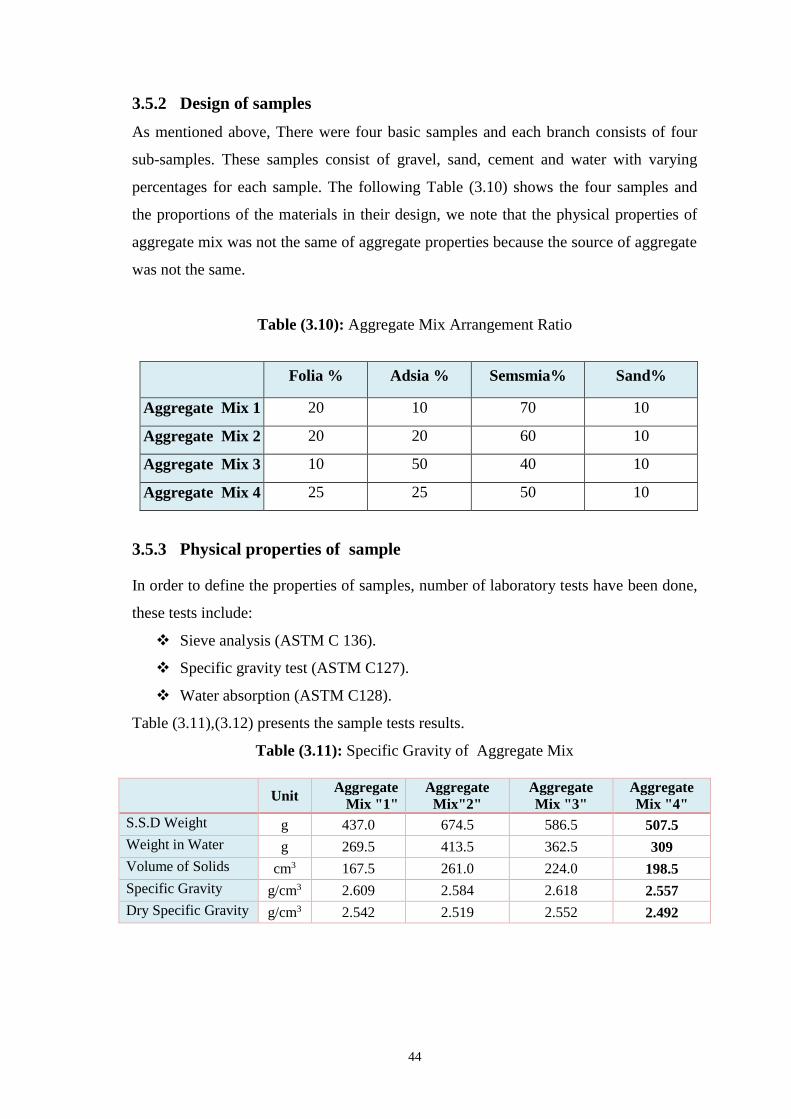
44
3.5.2 Design of samples
As mentioned above, There were four basic samples and each branch consists of four
sub-samples. These samples consist of gravel, sand, cement and water with varying
percentages for each sample. The following Table (3.10) shows the four samples and
the proportions of the materials in their design, we note that the physical properties of
aggregate mix was not the same of aggregate properties because the source of aggregate
was not the same.
Table (3.10): Aggregate Mix Arrangement Ratio
Folia % Adsia % Semsmia% Sand%
Aggregate Mix 1 20 10 70 10
Aggregate Mix 2 20 20 60 10
Aggregate Mix 3 10 50 40 10
Aggregate Mix 4 25 25 50 10
3.5.3 Physical properties of sample
In order to define the properties of samples, number of laboratory tests have been done,
these tests include:
Sieve analysis (ASTM C 136).
Specific gravity test (ASTM C127).
Water absorption (ASTM C128).
Table (3.11),(3.12) presents the sample tests results.
Table (3.11): Specific Gravity of Aggregate Mix
Aggregate
Mix "4"
Aggregate
Mix "3"
Aggregate
Mix"2"
Aggregate
Mix "1" Unit
507.5 586.5 674.5 437.0 g S.S.D Weight
309 362.5 413.5 269.5 g Weight in Water
198.5 224.0 261.0 167.5 cm3 Volume of Solids
2.557 2.618 2.584 2.609 g/cm3 Specific Gravity
2.492 2.552 2.519 2.542 g/cm3 Dry Specific Gravity

45
Table (3.12): Water Absorption Test of Samples
Aggregate
Mix "4"
Aggregate
Mix "3"
Aggregate
Mix "2"
Aggregate
Mix "1" Unit
507.5 586.5 674.5 437.0 g S.S.D Weight
495 572 658 426 g Oven Dry Weight
2.525 2.535 2.508 2.582 % Water Absorption
3.5.4 Sieve analysis of aggregate mix samples
In order to define the sieve analysis and according to specification (ASTM C136), we
collected the quantity of aggregate as arrangement ratio in Table (3.10), the sieve
analysis that performed on a four aggregate mix sample as shown at Table (3.13) to
Table (3.16).
Table (3.13): Sieve Analysis (Aggregate Mix #1)
Dry weight of sample before sieving = 3010g
% Passing Cumulative
% Retained
%
Retained
Weight
Retained (g)
Sieve Opening
Size (mm)
Sieve No.
100.00 0.0 0.00 0.0 25.00 1"
88.21 11.8 11.79 355.0 19.00 3/4"
64.29 35.7 23.92 720.0 12.50 1/2"
57.64 42.4 6.64 200.0 9.50 3/8"
13.95 86.0 43.69 1315.0 4.75 #4
1.83 98.2 12.13 15.0 2.36 #8
1.33 98.7 0.50 0.0 1.18 #16
1.33 98.7 0.00 0.0 0.60 #30
1.33 98.7 0.00 0.0 0.30 #50
1.33 98.7 0.00 0.0 0.15 #100
1.33 98.7 0.00 0.0 0.075 #200
0.0 100.0 1.33 40.0 0.00 pan

46
Figure (3.8): Gradation Curve –( Aggregate Mix#1)
Table (3.14): Sieve Analysis (Aggregate Mix #2)
Dry weight of sample before sieving = 2505g % Passing Cumulative
% Retained
% Retained Weight
Retained (g)
Sieve Opening
Size (mm)
Sieve No.
100.00 0.0 0.00 0.0 25.00 1"
86.63 13.4 13.37 355.0 19.00 3/4"
61.48 38.5 25.15 630.0 12.50 1/2"
51.5 48.5 9.98 250.0 9.50 3/8"
17.56 82.4 33.93 850.0 4.75 #4
2.79 97.2 14.77 370.0 2.36 #8
1.20 98.8 1.6 40.0 1.18 #16
1.20 98.8 0.00 0.0 0.60 #30
1.20 98.8 0.00 0.0 0.30 #50
1.20 98.8 0.00 0.0 0.15 #100
1.20 98.8 0.00 0.0 0.075 #200
0.0 100.0 1.20 30.0 0.00 pan
0.00
10.00
20.00
30.00
40.00
50.00
60.00
70.00
80.00
90.00
100.00
0.10 1.00 10.00 100.00
% P
assin
g
Sieve Size (mm)

47
Figure (3.9): Gradation Curve – ( Aggregate Mix #2)
Table (3.15): Sieve Analysis (Aggregate Mix #3)
Dry weight of sample before sieving = 2510g % Passing Cumulative
% Retained
% Retained Weight
Retained (g)
Sieve Opening
Size (mm)
Sieve No.
100.00 0.0 0.00 0.0 25.00 1"
95.62 4.4 4.38 110.0 19.00 3/4"
65.74 34.3 29.88 750.0 12.50 1/2"
40.84 59.2 24.9 625.0 9.50 3/8"
10.16 89.8 30.68 770.0 4.75 #4
1.99 98.0 8.17 205.0 2.36 #8
1.20 98.8 0.8 20.0 1.18 #16
1.20 98.8 0.00 0.0 0.60 #30
1.20 98.8 0.00 0.0 0.30 #50
1.20 98.8 0.00 0.0 0.15 #100
1.20 98.8 0.00 0.0 0.075 #200
0.0 100.0 1.20 30.0 0.00 pan
0.00
10.00
20.00
30.00
40.00
50.00
60.00
70.00
80.00
90.00
100.00
0.10 1.00 10.00 100.00
% P
assin
g
Sieve Size (mm)

48
Figure (3.10): Gradation Curve – (Aggregate Mix #3)
Table (3.16): Sieve Analysis (Aggregate Mix #4)
Dry weight of sample before sieving = 2510g % Passing Cumulative
% Retained
% Retained Weight
Retained (g)
Sieve Opening
Size (mm)
Sieve No.
100.00 0.0 0.00 0.0 25.00 1"
89.84 10.2 10.16 255.0 19.00 3/4"
60.56 39.4 29.28 735.0 12.50 1/2"
46.81 53.2 13.75 345.0 9.50 3/8"
14.34 85.7 32.47 815.0 4.75 #4
2.59 97.4 11.75 295.0 2.36 #8
1.39 98.6 1.2 30.0 1.18 #16
1.39 98.6 0.00 0.0 0.60 #30
1.39 98.6 0.00 0.0 0.30 #50
1.39 98.6 0.00 0.0 0.15 #100
1.39 98.6 0.00 0.0 0.075 #200
0.0 100.0 1.39 35.0 0.00 pan
0.00
10.00
20.00
30.00
40.00
50.00
60.00
70.00
80.00
90.00
100.00
0.10 1.00 10.00 100.00
% P
assin
g
Sieve Size (mm)

49
Figure (3.11): Gradation Curve – (Aggregate Mix #4)
3.5.5 Mixture design method
The design approach of Porous Interlock is mainly based on proper selection of
narrowly graded coarse aggregate and varying the paste volume until the target
properties are achieved.
The water content that should be used in Porous Interlock depends mainly on the
gradation and physical characteristics of aggregate as well as the cementitious materials
type and content.
A successful mix design for Porous interlock should consist of a balanced composition
of materials to ensure the best performance in terms of permeability, strength, and
durability.
The required quantity was calculated in each mixture for the possibility of producing
about 170 stone Interlock by using the three types of aggregate Folia, Adsia and
Semsimia, in addition to sand, cement and water according to the ratio to Table (3.10), The quantities of water and cement are set by reference to w/c ratio .
Table (3.17) shows the quantity of materials for each mix.
0.00
10.00
20.00
30.00
40.00
50.00
60.00
70.00
80.00
90.00
100.00
0.10 1.00 10.00 100.00
% P
assin
g
Sieve Size (mm)

50
Table (3.17): Material Samples Quantity
Concrete Mix Mixture ratio/ Kg.m-3
Aggregate Cement Water W/C Ratio
1-1 1564 187.7 61.94 0.33
1-2 1564 172.1 62 0.36
1-3 1564 156.4 61 0.39
1-4 1564 140.8 59.12 0.42
2-1 1564 187.7 67.57 0.36
2-2 1564 172.1 56.79 0.33
2-3 1564 156.4 65.69 0.42
2-4 1564 140.8 54.91 0.39
3-1 1564 187.7 73.2 0.39
3-2 1564 172.1 72.28 0.42
3-3 1564 156.4 51.61 0.33
3-4 1564 140.8 50.69 0.36
4-1 1564 187.7 78.83 0.42
4-2 1564 172.1 67.12 0.39
4-3 1564 156.4 56.3 0.36
4-4 1564 140.8 46.46 0.33
3.5.6 Mixing and processing samples
In this part of the research, the mixes were processed in local factory (The
Automatically Factory) in Gaza. in order to ensure the quality and preservation of the
required compaction for the stone. The mixes were manufactured in 20 × 10 × 8 cm
dimensions The following figures explain the stages of casting mix.
Figure (3.12) shows the materials used in the manufacture of porous interlock, which is
the folia, adsia and semsemia, whose properties and proportions of the use of mixtures
were identified in the previous tables.

51
Figure (3.12): Supplying used materials
Figure (3.13) shows the tool which through it the quantities used to produce a concrete
mix and weights are determined and the ratios used, the tool are an electronic balance
that is electronically controlled and given weights with high accuracy.
Figure (3.13): adjustment the weights of materials
Figure (3.14) show the mechanical machine used to perform the mechanical vibrate of
the concrete mix, is also used to make the necessary pressure to form the mixture and
the closure of pores, and it is done according to the ASTM specifications.

52
Figure(3.14): Compaction machine
Figure (3.15) show the Interlock samples after the production and the work of the
pressure necessary for the stone, and then moved to specific cells for the purpose of
water treatment, then transfer the samples to the laboratory to do all the necessary tests,
which will be presented in the next chapter.
Figure (3.15): Samples ready for processing

53
3.6 Infiltration Tests
It is the 3rd stage of testing, A design was developed to calculate the permeability of the
samples that have been processed. The design of experiment was constructed in a
1.0x1.0m with 0.25m depth from steel box. and Figure (3.16) shows the steel box that
constructed for the experiment, Figure (3.17), (3.18) shows cross section of
experimental box.
Figure (3.16): The experimental steel box

54
Figure (3.17): The experimental steel box of the permeable pavement, Figure (3.18): The schematic setup of the nozzles
3.6.1 Pavement construction
Figure (3.16) shows the steel box that constructed for the experiment. This was
constructed after completing the initial tests for interlock tiles and aggregate properties.
Figure (3.19) shows the interlock pavers sitting in experiment steel box. The joints
between the blocks were filled with cement mortar that used to Prevent water from
flowing through the joints as showmen in Figure (3.20). And the pattern used was
stretcher bond (90°).

55
Figure (3.19):Interlock pavement (stretcher bond 90° pattern)
Figure (3.20): Joints filled with mortar (stretcher bond 90° pattern)

56
3.6.2 Rainfall simulator installation
Figure (3.21) of the steel box were installed after completing the construction of the
pavement. Finally, the funnel was fixed under the steel box to collect the infiltrated
water. As mentioned previously, the rainfall simulator (Figures (3.22) & (3.23)) was
placed with steel grid carrying the 25 nozzles installed at 80 cm from the surface of the
pavement.The water flows through the joints of blocks was collected from underneath
the pavement a funnel Figure (3.24).
The control in the quantity of water that infiltrated on pavement with valve more time to
reach to the 60Liter of water in 60 minutes, The control of water quantity is manually
because lack of availability mechanical control, and we chose the quantity of water 60
liter and time 60 minutes to reach the medium intensity rate 60mm/hr as situation of
rainy status in the Gaza Strip .
Figure (3.21): Rainfall simulator and laboratory pavement model box

57
Figure (3.22): The 25 evenly setup sprays
Figure (3.23): Infiltration test on the constructed permeable pavement

58
Figure (3.24):Infiltrated water out through permeable pavement
3.6.3 Rainfall simulator intensity
The rainfall intensity RI simulation consist of (60mm/h), rainfall storms of uniform
intensities where the taken from curves of return periods for the 16 samples.

59
Chapter (4)
Results and discussion

60
4.1 Introduction
Results of experimental work were obtained and discussed to achieve the study
objectives, which include studying the properties of aggregates, cement, and water on
the permeability of water in porous interlock pavement.
The results are presented in this chapter in two stages. First, recording all results of 16
processed samples as compressive strength, absorption and density. Second stage shows
the permeability percentage of water with different interlock samples.
4.2 Result of experimental scenarios
In the previous chapter, after conducting all the tests for the materials needed for
processing the samples, we manufactured the samples. After processing the samples, we
divided the samples into two parts. The first part of the samples was immersed in water
for 24 hours to determine the percentage of absorption. The second part of the samples
was treated with water for 28 days. to know the compressive strength .
4.2.1 Result of Compressive Strength and Absorption for 16 samples
The result of average Compressive Strength and average Absorption is record in
Table (4.1). The average results of 10 stones result are show in appendix B
Palestine Standards Institution (PSI) shows the characteristics and specifications as:
The compressive strength of concrete block has been stated to range between 45
and 50 MPa.
The maximum absorption when placed in water for 10 minutes no more than 2%
and when placed in water for 24 hour no more than 5%.

61
Table (4.1): Compressive Strength, and Absorption Result
Serial No Concrete Mix No
Average Compressive
Strength at 28 days
)2kg/cm(
Average Absorption
%
1 1-1 370 2.46
2 1-2 336 2.48
3 1-3 312 2.57
4 1-4 286 2.73
5 2-1 277 2.78
6 2-2 297 2.66
7 2-3 229 3.36
8 2-4 246 3.12
9 3-1 316 2.55
10 3-2 301 2.60
11 3-2 335 2.49
12 3-4 320 2.52
13 4-1 231 3.28
14 4-2 249 2.91
15 4-3 252 2.88
16 4-4 261 2.82
4.3 Result of permeability scenarios
The simulation consist of (60mm/h) rainfall storms of uniform intensities to test the
infiltration rate. The flow rate of 60 mm/h was suitable to flow through the nozzles.
The nozzles of the rainfall simulator were placed directly above the experimental area.
The funnel underneath the pavement is also placed within the area to collect water.
In order to obtain the infiltration characteristics through the bedding layer and flow
through the whole pavement structure for rainfall event, the water flow through the
bottom of the pavement was collected at 1 minute interval.

62
4.3.1 Result of outflow at rainfall intensity=60 mm/h (Sample 1-1)
The result of cumulative outflow is record in Table (4.2) and permeability percentage %
for sample (1-1) was calculated.
Table (4.2): Cumulative outflow for sample (1-1) at (RI=60 mm/h)
Cumulative outflow (L) Inflow (L) Time (min)
23.46 60.00 60
39.1 permeability percentage (%)
Figure (4.1) illustrates the results for sample (1-1) during the intensity of water = 60
mm/h.
Figure(4.1): Outflow results for sample (1-1) at intensity of water (60 mm/h)
0
2
4
6
8
10
12
14
16
18
20
22
24
26
28
30
0 5 10 15 20 25 30 35 40 45 50 55 60
Ou
t fl
ow
(L)
Time(min)

63
4.3.2 Result of outflow at rainfall intensity=60 mm/h (Sample 1-2)
The result of cumulative outflow is record in Table (4.3) and permeability percentage %
for sample (1-2) was calculated.
Table (4.3): Cumulative outflow for sample (1-2) at (RI=60 mm/h)
Cumulative outflow (L) Inflow (L) Time (min)
24.67 60.00 60
41.12 permeability percentage (%)
Figure (4.2) illustrates the results for sample (1-2) during the intensity of water = 60
mm/h.
Figure(4.2): Outflow results for sample (1-2) at intensity of water (60 mm/h)
0
2
4
6
8
10
12
14
16
18
20
22
24
26
28
30
0 5 10 15 20 25 30 35 40 45 50 55 60
Ou
t fl
ow
(L)
Time(min)

64
4.3.3 Result of outflow at rainfall intensity=60 mm/h (Sample 1-3)
The result of cumulative outflow is record in Table (4.4) and permeability percentage %
for sample (1-3) was calculated.
Table (4.4): Cumulative outflow for sample (1-3) at (RI=60 mm/h)
Cumulative outflow (L) Inflow (L) Time (min)
25.66 60.00 60
42.77 permeability percentage (%)
5
Figure (4.3) illustrates the results for sample (1-3) during the intensity of water = 60
mm/h.
Figure(4.3): Outflow results for sample (1-3) at intensity of water (60 mm/h)
0
2
4
6
8
10
12
14
16
18
20
22
24
26
28
30
0 5 10 15 20 25 30 35 40 45 50 55 60
Ou
t fl
ow
(L)
Time(min)

65
4.3.4 Result of outflow at rainfall intensity=60 mm/h (Sample 1-4)
The result of cumulative outflow is record in Table (4.5) and permeability percentage %
for sample (1-4) was calculated.
Table (4.5): Cumulative outflow for sample (1-3) at (RI=60 mm/h)
Cumulative outflow (L) Inflow (L) Time (min)
26.72 60.00 60
44.53 permeability percentage (%)
4
Figure (4.4) illustrates the results for sample (1-4) during the intensity of water = 60
mm/h.
Figure(4.4): Outflow results for sample (1-4) at intensity of water (60 mm/h)
0
2
4
6
8
10
12
14
16
18
20
22
24
26
28
30
0 5 10 15 20 25 30 35 40 45 50 55 60
Ou
t fl
ow
(L)
Time(min)

66
4.3.5 Result of outflow at rainfall intensity=60 mm/h (Sample 2-1)
The result of cumulative outflow is record in Table (4.6) and permeability percentage %
for sample (2-1) was calculated.
Table (4.6): Cumulative outflow for sample (2-1) at (RI=60 mm/h)
Cumulative outflow (L) Inflow (L) Time (min)
26.81 60.00 60
44.68 permeability percentage (%)
5
Figure (4.5) illustrates the results for sample (2-1) during the intensity of water = 60
mm/h.
Figure(4.5): Outflow results for sample (2-1) at intensity of water (60 mm/h)
0
2
4
6
8
10
12
14
16
18
20
22
24
26
28
30
0 5 10 15 20 25 30 35 40 45 50 55 60
Ou
t fl
ow
(L)
Time(min)

67
4.3.6 Result of outflow at rainfall intensity=60 mm/h (Sample 2-2)
The result of cumulative outflow is record in Table (4.7) and permeability percentage %
for sample (2-2) was calculated.
Table (4.7): Cumulative outflow for sample (2-2) at (RI=60 mm/h)
Cumulative outflow (L) Inflow (L) Time (min)
25.99 60.00 60
43.32 permeability percentage (%)
6
Figure (4.6) illustrates the results for sample (2-2) during the intensity of water = 60
mm/h.
Figure(4.6): Outflow results for sample (2-2) at intensity of water (60 mm/h)
0
2
4
6
8
10
12
14
16
18
20
22
24
26
28
30
0 5 10 15 20 25 30 35 40 45 50 55 60
Ou
t fl
ow
(L)
Time(min)

68
4.3.7 Result of outflow at rainfall intensity=60 mm/h (Sample 2-3)
The result of cumulative outflow is record in Table (4.8) and permeability percentage %
for sample (2-3) was calculated.
Table (4.8): Cumulative outflow for sample (2-3) at (RI=60 mm/h)
Cumulative outflow (L) Inflow (L) Time (min)
27.86 60.00 60
46.43 permeability percentage (%)
7
Figure (4.7) illustrates the results for sample (2-3) during the intensity of water = 60
mm/h.
Figure(4.7): Outflow results for sample (2-3) at intensity of water (60 mm/h)
0
2
4
6
8
10
12
14
16
18
20
22
24
26
28
30
0 5 10 15 20 25 30 35 40 45 50 55 60
Ou
t fl
ow
(L)
Time(min)

69
4.3.8 Result of outflow at rainfall intensity=60 mm/h (Sample 2-4)
The result of cumulative outflow is record in Table (4.9) and permeability percentage %
for sample (2-4) was calculated.
Table (4.9): Cumulative outflow for sample (2-4) at (RI=60 mm/h)
Cumulative outflow (L) Inflow (L) Time (min)
27.04 60.00 60
45.07 permeability percentage (%)
8
Figure (4.8) illustrates the results for sample (2-4) during the intensity of water = 60
mm/h.
Figure(4.8): Outflow results for sample (2-4) at intensity of water (60 mm/h)
0
2
4
6
8
10
12
14
16
18
20
22
24
26
28
30
0 5 10 15 20 25 30 35 40 45 50 55 60
Ou
t fl
ow
(L)
Time(min)

70
4.3.9 Result of outflow at rainfall intensity=60 mm/h (Sample 3-1)
The result of cumulative outflow is record in Table (4.10) and permeability percentage
% for sample (3-1) was calculated.
Table (4.10): Cumulative outflow for sample (3-1) at (RI=60 mm/h)
Cumulative outflow (L) Inflow (L) Time (min)
23.61 60.00 60
39.35 permeability percentage (%)
9
Figure (4.9) illustrates the results for sample (3-1) during the intensity of water = 60
mm/h.
Figure(4.9): Outflow results for sample (3-1) at intensity of water (60 mm/h)
0
2
4
6
8
10
12
14
16
18
20
22
24
26
28
30
0 5 10 15 20 25 30 35 40 45 50 55 60
Ou
t fl
ow
(L)
Time(min)

71
4.3.10 Result of outflow at rainfall intensity=60 mm/h (Sample 3-2)
The result of cumulative outflow is record in Table (4.11) and permeability percentage
% for sample (3-2) was calculated.
Table (4.11): Cumulative outflow for sample (3-2) at (RI=60 mm/h)
Cumulative outflow (L) Inflow (L) Time (min)
24.91 60.00 60
41.52 permeability percentage (%)
10
Figure (4.10) illustrates the results for sample (3-2) during the intensity of water = 60
mm/h.
Figure(4.10): Outflow results for sample (3-2) at intensity of water (60 mm/h)
0
2
4
6
8
10
12
14
16
18
20
22
24
26
28
30
0 5 10 15 20 25 30 35 40 45 50 55 60
Ou
t fl
ow
(L)
Time(min)

72
4.3.11 Result of outflow at rainfall intensity=60 mm/h (Sample 3-3)
The result of cumulative outflow is record in Table (4.12) and permeability percentage
% for sample (3-3) was calculated.
Table (4.12): Cumulative outflow for sample (3-3) at (RI=60 mm/h)
Cumulative outflow (L) Inflow (L) Time (min)
22.39 60.00 60
37.32 permeability percentage (%)
11
Figure (4.11) illustrates the results for sample (3-3) during the intensity of water = 60
mm/h.
Figure(4.11): Outflow results for sample (3-3) at intensity of water (60 mm/h)
0
2
4
6
8
10
12
14
16
18
20
22
24
26
28
30
0 5 10 15 20 25 30 35 40 45 50 55 60
Ou
t fl
ow
(L)
Time(min)

73
4.3.12 Result of outflow at rainfall intensity=60 mm/h (Sample 3-4)
The result of cumulative outflow is record in Table (4.13) and permeability percentage
% for sample (3-4) was calculated.
Table (4.13): Cumulative outflow for sample (3-4) at (RI=60 mm/h)
Cumulative outflow (L) Inflow (L) Time (min)
23 60.00 60
38.33 permeability percentage (%)
12
Figure (4.12) illustrates the results for sample (3-4) during the intensity of water = 60
mm/h.
Figure(4.12): Outflow results for sample (3-4) at intensity of water (60 mm/h)
0
2
4
6
8
10
12
14
16
18
20
22
24
26
28
30
0 5 10 15 20 25 30 35 40 45 50 55 60
Ou
t fl
ow
(L)
Time(min)

74
4.3.13 Result of outflow at rainfall intensity=60 mm/h (Sample 4-1)
The result of cumulative outflow is record in Table (4.14) and permeability percentage
% for sample (4-1) was calculated.
Table (4.14): Cumulative outflow for sample (4-1) at (RI=60 mm/h)
Cumulative outflow (L) Inflow (L) Time (min)
29.95 60.00 60
49.92 permeability percentage (%)
13
Figure (4.13) illustrates the results for sample (4-1) during the intensity of water = 60
mm/h.
Figure(4.13): Outflow results for sample (4-1) at intensity of water (60 mm/h)
0
2
4
6
8
10
12
14
16
18
20
22
24
26
28
30
0 5 10 15 20 25 30 35 40 45 50 55 60
Ou
t fl
ow
(L)
Time(min)

75
4.3.14 Result of outflow at rainfall intensity=60 mm/h (Sample 4-2)
The result of cumulative outflow is record in Table (4.15) and permeability percentage
% for sample (4-2) was calculated.
Table (4.15): Cumulative outflow for sample (4-2) at (RI=60 mm/h)
Cumulative outflow (L) Inflow (L) Time (min)
28.62 60.00 60
47.7 permeability percentage (%)
14
Figure (4.14) illustrates the results for sample (4-2) during the intensity of water = 60
mm/h.
Figure(4.14): Outflow results for sample (4-2) at intensity of water (60 mm/h)
0
2
4
6
8
10
12
14
16
18
20
22
24
26
28
30
0 5 10 15 20 25 30 35 40 45 50 55 60
Ou
t fl
ow
(L)
Time(min)

76
4.3.15 Result of outflow at rainfall intensity=60 mm/h (Sample 4-3)
The result of cumulative outflow is record in Table (4.16) and permeability percentage
% for sample (4-3) was calculated.
Table (4.16): Cumulative outflow for sample (4-3) at (RI=60 mm/h)
Cumulative outflow (L) Inflow (L) Time (min)
26.19 60.00 60
43.65 permeability percentage (%)
15
Figure (4.15) illustrates the results for sample (4-3) during the intensity of water = 60
mm/h.
Figure(4.15): Outflow results for sample (4-3) at intensity of water (60 mm/h)
0
2
4
6
8
10
12
14
16
18
20
22
24
26
28
30
0 5 10 15 20 25 30 35 40 45 50 55 60
Ou
t fl
ow
(L)
Time(min)

77
4.3.16 Result of outflow at rainfall intensity=60 mm/h (Sample 4-4)
The result of cumulative outflow is record in Table (4.17) and permeability percentage
% for sample (4-4) was calculated.
Table (4.17): Cumulative outflow for sample (4-4) at (RI=60 mm/h)
Cumulative outflow (L) Inflow (L) Time (min)
25.11 60.00 60
41.85 permeability percentage (%)
16
Figure (4.16) illustrates the results for sample (4-4) during the intensity of water = 60
mm/h.
Figure(4.16): Outflow results for sample (4-4) at intensity of water (60 mm/h)
0
2
4
6
8
10
12
14
16
18
20
22
24
26
28
30
0 5 10 15 20 25 30 35 40 45 50 55 60
Ou
t fl
ow
(L)
Time(min)

78
4.4 Discussion
After the completion of the necessary tests in the laboratory on 16 samples, the
compressive strength, absorption and the permeability, and these results were presented
in the previous tables, we will discuss these result and compare with previous studies.
As shown in the table (4.4), the results of the compressive strength were range between
229-370 kg/cm2, and it was a good results compared to the Palestinian specifications in
the case of a common interlock, and the reason in these results are:
The percentage of voids between aggregate that range from 40-45%, which is
shown in compressive strength results in mixtures # 2,4.
Also water and cement ratios were controlled in the compressive strength
values, where we note that the lowest value of compressive strength in sample
2-3, and the highest value in sample 1-1.
For the results of permeability it range from (37-50%), that according to the previous
tables, and after discussion and analysis we note that:
The result of permeability were Converged.
The highest values of permeability were in mixture No. 4 where the percentage
of folia aggregate is the largest percentage among mixtures and therefore the
percentage of voids are high.
In the case of large water cement ratio, the permeability is low.
Since one of the objectives of the research is to calculate the amount of permeability, it
means that the best mixture is the mixture No. 4-1, where the highest permeability
49.92.

79
Chapter (5)
Conclusions and Recommendations

80
5.1 Conclusions
The following conclusions can be drawn:
a) The study has shown the possibility of producing and using porous interlock in
Gaza Strip and studying the infiltration rate of water through this Interlock and
reduce the amount of water accumulated on the surface as runoff water as much
as possible by using a variety of experiences.
b) It was found that it is possible to use new types of aggregate such as Folia and
Adasia, which are not used in the traditional Interlock industry and in varying
proportions.
c) Through the study, identified four basic samples with varying percentages of the
three types of Aggregate Folia, Adasia, and Somsmia, with a change in the
percentage of cement and water. This is a good indicator for researchers that it is
possible to use other percentages of the aggregate and produce other samples for
research and finding other results.
d) There is a possibility to produce and manufacture all the available forms of
Interlock in the local markets and be permeable for water, but in this study
restricted Interlock Square 10 × 20 cm, because of the difficulty of changing the
templates used during the tests because the cost of time and effort and money to
change.
e) The results show that there is an inverse relationship between compressive
strength and permeability, as the greater the compressive strength of the sample,
the less permeability.
f) The results showed that the permeability rate ranged between (37%-50%) and
the results were obtained and the joints between the interlock are closed with
mortar but if the joints through the testing are openings, was possible to obtain
the results of the multiplication of permeability.
g) In this research, a medium percentage of intensity rate was used, which is 60
mm/h, but it is possible to use other rates such as (15mm/h, 45mm/h, 120mm/h)
and finding other results, which opens the way for other researchers to complete
other research on the subject.

81
5.2 Recommendations
a) In order to approve and confirm the success and integrity of the results of the
laboratory, these results should be applied on the field and also for an integrated
understanding of the subject.
b) Through the results that have obtained, especially the compressive strength
results of the samples, study recommends to use of porous interlock in areas
with lights load tolerance such as playgrounds, parking, and corridors.
c) It is important to get benefit from amounts of water that is collected and not
neglected then, re-injected into groundwater aquifer to reduce the water
problem.
d) It is recommended to increase the efficiency of water leakage through porous
Interlock to be layers under the porous interlock layers more porosity by
replacing the layer of base coarse with a layer of gravel and the use of geotextile
and the use of pipes under these layers to collect water.
e) It is recommended to conduct similar studies about making mix concrete tile that
has special specification to permeable water through the tiles and consist of
compounds with water permeability properties.
f) It is recommended to use additives during sample casting to increase sample
compressive strength.
g) Government, institutions, municipalities and researchers should integrate efforts
toward preparing and implementing water management plan reinforcing the
environmental sustainability by taking and support important issues to
development the infrastructure.
82
References
Adams, M, 2006, ‘Sustainable Site Design, Porous Pavement and Innovative Storm
water Techniques, Cahill Associates, Inc., Environmental Consultants, American Public
Works Association.
An Cheng, Hui-Mi Hsu, Sao-Jeng Chao, and Kae-Long Lin, 2011, Experimental Study
on Properties of Pervious Concrete Made with Recycled Aggregate, Chinese Society of
Pavement Engineering.
Bruce K. Ferguson, 2006, "Porous Pavement : The Making Of Progress in Technology
and Design , School of Environmental Design, University of Georgia Athens, Georgia.
Bruce K. Ferguson, 2007, Porous Pavement in Georgia, University of Georgia.
Bruce K. Ferguson, 2005, Porous Pavements: The Overview, University of Georgia
School of Environmental Design.
Carmen T. Agouridis, Jonathan A. Villines, and Joe D. Luck, 2011, Permeable
Pavement for Stormwater Management, University of Kentucky College of Agriculture,
Lexington.
Coastal Municipalities Water Utility (CMWU) Annual Report on Water Status in the
Gaza Strip, 2010, Summary about Water and Wastewater Situation in Gaza Strip, Gaza,
Palestine.
Federal Highway Administration (FHWA), 2015,Office of Asset Management
Pavement and Construction, Permeable Interlocking Concrete Pavement.
H.M. Imran, Shatirah Akib and Mohamed Rehan Karim, 2013," Permeable pavement
and stormwater management systems", Department of Civil Engineering, Faculty of
Engineering, University of Malaya, Malaysia.
Abustan . I, Hamzah. O, Rashid . M, 2012, Review of Permeble Pavement System in
Malaysia Condition, School of Civil Engineering, Engineering Campus, University
Sains Malaysia.
Interlocking Concrete Pavement Institute (ICPI), 2015,Construction of Interlocking
Concrete Pavements, Canda.

83
Jendia .S, Madhoun . M, 2014, Study the Effect of Joints, Block Shape and Pavement
Pattern on the Permeability of Concrete Block Pavement (Interlock Pavement), Gaza,
Palestine.
K.G.Sharp, 1979, An Initial Study into Concrete Block Paving, Australian Road
Research Board , Australia.
Khalaf, A., 2005, ‘Assessment of Rainwater Losses due to Urban Expansion of Gaza
Strip, M.Sc Thesis, Islamic University of Gaza, Palestine.
Aslantas . O, 2004, A study on Abrasion Resistance of Concrete Paving Blocks, Middle
East Technical University, Turkey.
Palestinian Standard Certificates (PSI and PSM) for block and tiles, Palestinian
Standard PS 72, 1997.
Permeable Pavement Fact Sheet Information for Howard County, Maryland
Homeowners, 2007, University of Maryland.
Rabah . F, 2008, ‘Sanitary Engineering Lecturer- Design of Storm Water Drainge
System in Gaza City.
Hamdan . S, 2012, Artificial Recharge of Groundwater with Stormwater as a New
Water Resource - Case Study of the Gaza Strip, Palestine ,Technical University Berlin .
Terry Lucke, 2014, Using Drainage Slots in Permeable Paving Blocks to Delay the
Effects of Clogging: Proof of Concept Study, Stormwater Research Group, School of
Science and Engineering, University of the Sunshine Coast, Sippy Downs, Australia.
Toronto and Region Conservation Authority, 2011, Low Impact Development Storm
water Management Planning and Design Guide.
Terry Lucke, Richard White, Peter Nichols, and Sönke Borgwardt, 2015, A Simple
Field Test to Evaluate the Maintenance Requirements of Permeable Interlocking
Concrete Pavements, Stormwater Research Group, University of the Sunshine Coast,
Sippy Downs, Queensland, Australia, Büro BWB Norderstedt, Kattendorf, Germany.
Upana Rath, 2007, Structural Behavior of Interlocking Concrete Block Pavement,
Department of Civil Engineering National Institute of Technology, Pourkela.
William F. Hunt, Kelly A. Collins, 2007, Permeable Pavement: Research Update and
Design Implications , North Carolina State University.

84
WisDOT Southeast Region, 2012, Comparison of Permeable Pavement Types:
Hydrology, Design, Installation, Maintenance and Cost .

85
Appendices

86
Appendix (A)
Porosity Results

87
Result of permeability for Sample (1-1) at rainfall intensity=60 mm/h
Table (A.1): Cumulative outflow for sample 1-1 at (RI=60 mm/h)
Time (min) Inflow (L) Cumulative outflow (L)
1 st 1 0
2 nd 2 0
3 rd 3 0.12
4 th 4 0.45
5 th 5 0.81
6 th 6 1.2
7 th 7 1.59
8 th 8 1.98
9 th 9 2.37
10 th 10 2.76
11 th 11 3.21
12 th 12 3.66
13 th 13 4.08
14 th 14 4.5
15 th 15 4.92
16 th 16 5.34
17 th 17 5.75
18 th 18 6.16
19 th 19 6.57
20 th 20 6.98
21 st 21 7.4
22 nd 22 7.81
23 rd 23 8.22
24 th 24 8.63
25 th 25 9.04
26 th 26 9.46
27 th 27 9.87
28 th 28 10.28
29 th 29 10.69
30 th 30 11.1
31 st 31 11.52
32 nd 32 11.93
33 rd 33 12.34

88
Time (min) Inflow (L) Cumulative outflow (L)
34 th 34 12.75
35 th 35 13.16
36 th 36 13.58
37 th 37 13.99
38 th 38 14.4
39 th 39 14.81
40 th 40 15.22
41 st 41 15.64
42 nd 42 16.05
43 rd 43 16.46
44 th 44 16.87
45 th 45 17.28
46 th 46 17.7
47 th 47 18.11
48 th 48 18.52
49 th 49 18.93
50 th 50 19.34
51 st 51 19.76
52 nd 52 20.17
53 rd 53 20.58
54 th 54 20.99
55 th 55 21.4
56 th 56 21.82
57 th 57 22.23
58 th 58 22.64
59 th 59 23.05
60 th 60 23.46
permeability percentage (%) 39.10

89
Result of permeability for Sample (1-2) at rainfall intensity=60 mm/h
Table (A.2): Cumulative outflow for sample 1-2 at (RI=60 mm/h)
Time (min) Inflow (L) Cumulative outflow (L)
1 st 1 0
2 nd 2 0
3 rd 3 0.2
4 th 4 0.5
5 th 5 0.85
6 th 6 1.17
7 th 7 1.48
8 th 8 1.79
9 th 9 2.23
10 th 10 2.67
11 th 11 3.11
12 th 12 3.55
13 th 13 3.99
14 th 14 4.43
15 th 15 4.87
16 th 16 5.31
17 th 17 5.75
18 th 18 6.19
19 th 19 6.63
20 th 20 7.07
21 st 21 7.51
22 nd 22 7.95
23 rd 23 8.39
24 th 24 8.83
25 th 25 9.27
26 th 26 9.71
27 th 27 10.15
28 th 28 10.59
29 th 29 11.03
30 th 30 11.47
31 st 31 11.91
32 nd 32 12.35
33 rd 33 12.79

90
Time (min) Inflow (L) Cumulative outflow (L)
34 th 34 13.23
35 th 35 13.67
36 th 36 14.11
37 th 37 14.55
38 th 38 14.99
39 th 39 15.43
40 th 40 15.87
41 st 41 16.31
42 nd 42 16.75
43 rd 43 17.19
44 th 44 17.63
45 th 45 18.07
46 th 46 18.51
47 th 47 18.95
48 th 48 19.39
49 th 49 19.83
50 th 50 20.27
51 st 51 20.71
52 nd 52 21.15
53 rd 53 21.59
54 th 54 22.03
55 th 55 22.47
56 th 56 22.91
57 th 57 23.35
58 th 58 23.79
59 th 59 24.23
60 th 60 24.67
permeability percentage (%) 41.12

91
Result of permeability for Sample (1-3) at rainfall intensity=60 mm/h
Table (A.3): Cumulative outflow for sample 1-3 at (RI=60 mm/h)
Time (min) Inflow (L) Cumulative outflow (L)
1 st 1 0
2 nd 2 0.01
3 rd 3 0.25
4 th 4 0.59
5 th 5 0.97
6 th 6 1.34
7 th 7 1.81
8 th 8 2.26
9 th 9 2.71
10 th 10 3.16
11 th 11 3.61
12 th 12 4.06
13 th 13 4.51
14 th 14 4.96
15 th 15 5.41
16 th 16 5.86
17 th 17 6.31
18 th 18 6.76
19 th 19 7.21
20 th 20 7.66
21 st 21 8.11
22 nd 22 8.56
23 rd 23 9.01
24 th 24 9.46
25 th 25 9.91
26 th 26 10.36
27 th 27 10.81
28 th 28 11.26
29 th 29 11.71
30 th 30 12.16
31 st 31 12.61
32 nd 32 13.06
33 rd 33 13.51

92
Time (min) Inflow (L) Cumulative outflow (L)
34 th 34 13.96
35 th 35 14.41
36 th 36 14.86
37 th 37 15.31
38 th 38 15.76
39 th 39 16.21
40 th 40 16.66
41 st 41 17.11
42 nd 42 17.56
43 rd 43 18.01
44 th 44 18.46
45 th 45 18.91
46 th 46 19.36
47 th 47 19.81
48 th 48 20.26
49 th 49 20.71
50 th 50 21.16
51 st 51 21.61
52 nd 52 22.06
53 rd 53 22.51
54 th 54 22.96
55 th 55 23.41
56 th 56 23.86
57 th 57 24.31
58 th 58 24.76
59 th 59 25.21
60 th 60 25.66
permeability percentage (%) 42.77
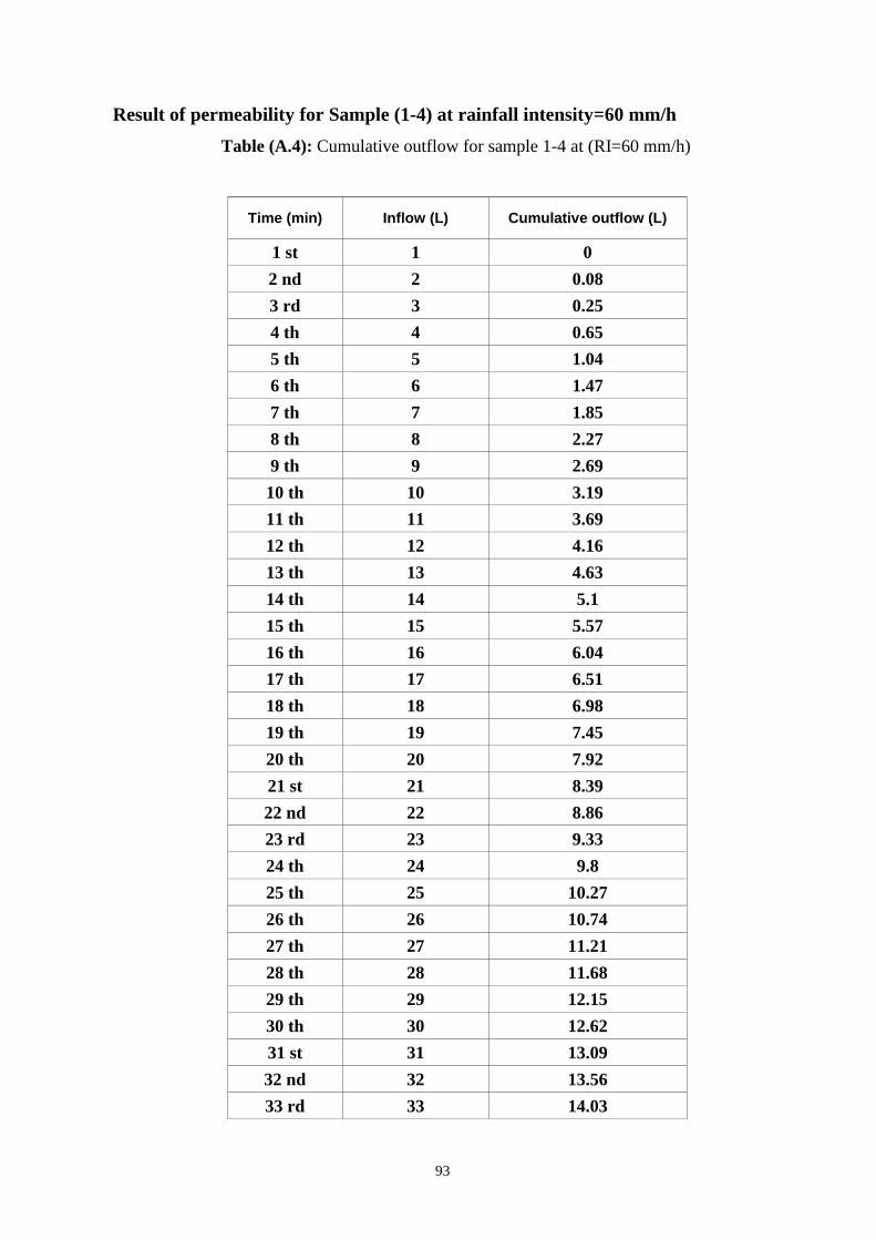
93
Result of permeability for Sample (1-4) at rainfall intensity=60 mm/h
Table (A.4): Cumulative outflow for sample 1-4 at (RI=60 mm/h)
Time (min) Inflow (L) Cumulative outflow (L)
1 st 1 0
2 nd 2 0.08
3 rd 3 0.25
4 th 4 0.65
5 th 5 1.04
6 th 6 1.47
7 th 7 1.85
8 th 8 2.27
9 th 9 2.69
10 th 10 3.19
11 th 11 3.69
12 th 12 4.16
13 th 13 4.63
14 th 14 5.1
15 th 15 5.57
16 th 16 6.04
17 th 17 6.51
18 th 18 6.98
19 th 19 7.45
20 th 20 7.92
21 st 21 8.39
22 nd 22 8.86
23 rd 23 9.33
24 th 24 9.8
25 th 25 10.27
26 th 26 10.74
27 th 27 11.21
28 th 28 11.68
29 th 29 12.15
30 th 30 12.62
31 st 31 13.09
32 nd 32 13.56
33 rd 33 14.03

94
Time (min) Inflow (L) Cumulative outflow (L)
34 th 34 14.5
35 th 35 14.97
36 th 36 15.44
37 th 37 15.91
38 th 38 16.38
39 th 39 16.85
40 th 40 17.32
41 st 41 17.79
42 nd 42 18.26
43 rd 43 18.73
44 th 44 19.2
45 th 45 19.67
46 th 46 20.14
47 th 47 20.61
48 th 48 21.08
49 th 49 21.55
50 th 50 22.02
51 st 51 22.49
52 nd 52 22.96
53 rd 53 23.43
54 th 54 23.9
55 th 55 24.37
56 th 56 24.84
57 th 57 25.31
58 th 58 25.78
59 th 59 26.25
60 th 60 26.72
permeability percentage (%) 44.53

95
Result of permeability for Sample (2-1) at rainfall intensity=60 mm/h
Table (A.5): Cumulative outflow for sample 2-1 at (RI=60 mm/h)
Time (min) Inflow (L) Cumulative outflow (L)
1 st 1 0
2 nd 2 0.15
3 rd 3 0.35
4 th 4 0.55
5 th 5 0.87
6 th 6 1.09
7 th 7 1.31
8 th 8 1.78
9 th 9 2.25
10 th 10 2.77
11 th 11 3.17
12 th 12 3.76
13 th 13 4.31
14 th 14 4.82
15 th 15 5.27
16 th 16 5.69
17 th 17 6.17
18 th 18 6.65
19 th 19 7.13
20 th 20 7.61
21 st 21 8.09
22 nd 22 8.57
23 rd 23 9.05
24 th 24 9.53
25 th 25 10.01
26 th 26 10.49
27 th 27 10.97
28 th 28 11.45
29 th 29 11.93
30 th 30 12.41
31 st 31 12.89
32 nd 32 13.37
33 rd 33 13.85
34 th 34 14.33

96
Time (min) Inflow (L) Cumulative outflow (L)
35 th 35 14.81
36 th 36 15.29
37 th 37 15.77
38 th 38 16.25
39 th 39 16.73
40 th 40 17.21
41 st 41 17.69
42 nd 42 18.17
43 rd 43 18.65
44 th 44 19.13
45 th 45 19.61
46 th 46 20.09
47 th 47 20.57
48 th 48 21.05
49 th 49 21.53
50 th 50 22.01
51 st 51 22.49
52 nd 52 22.97
53 rd 53 23.45
54 th 54 23.93
55 th 55 24.41
56 th 56 24.89
57 th 57 25.37
58 th 58 25.85
59 th 59 26.33
60 th 60 26.81
permeability percentage (%) 44.68

97
Result of permeability for Sample (2-2) at rainfall intensity=60 mm/h
Table (A.6): Cumulative outflow for sample 2-2 at (RI=60 mm/h)
Time (min) Inflow (L) Cumulative outflow (L)
1 st 1 0
2 nd 2 0.1
3 rd 3 0.35
4 th 4 0.65
5 th 5 0.95
6 th 6 1.28
7 th 7 1.63
8 th 8 2.02
9 th 9 2.46
10 th 10 2.91
11 th 11 3.45
12 th 12 3.91
13 th 13 4.37
14 th 14 4.83
15 th 15 5.29
16 th 16 5.75
17 th 17 6.21
18 th 18 6.67
19 th 19 7.13
20 th 20 7.59
21 st 21 8.05
22 nd 22 8.51
23 rd 23 8.97
24 th 24 9.43
25 th 25 9.89
26 th 26 10.35
27 th 27 10.81
28 th 28 11.27
29 th 29 11.73
30 th 30 12.19
31 st 31 12.65
32 nd 32 13.11

98
Time (min) Inflow (L) Cumulative outflow (L)
33 rd 33 13.57
34 th 34 14.03
35 th 35 14.49
36 th 36 14.95
37 th 37 15.41
38 th 38 15.87
39 th 39 16.33
40 th 40 16.79
41 st 41 17.25
42 nd 42 17.71
43 rd 43 18.17
44 th 44 18.63
45 th 45 19.09
46 th 46 19.55
47 th 47 20.01
48 th 48 20.47
49 th 49 20.93
50 th 50 21.39
51 st 51 21.85
52 nd 52 22.31
53 rd 53 22.77
54 th 54 23.23
55 th 55 23.69
56 th 56 24.15
57 th 57 24.61
58 th 58 25.07
59 th 59 25.53
60 th 60 25.99
permeability percentage (%) 43.32

99
Result of permeability for Sample (2-3) at rainfall intensity=60 mm/h
Table (A.7): Cumulative outflow for sample 2-3 at (RI=60 mm/h)
Time (min) Inflow (L) Cumulative outflow (L)
1 st 1 0
2 nd 2 0.1
3 rd 3 0.35
4 th 4 0.65
5 th 5 0.95
6 th 6 1.35
7 th 7 2.03
8 th 8 2.43
9 th 9 2.98
10 th 10 3.38
11 th 11 3.81
12 th 12 4.18
13 th 13 4.51
14 th 14 4.84
15 th 15 5.17
16 th 16 5.64
17 th 17 5.97
18 th 18 6.32
19 th 19 6.67
20 th 20 7.02
21 st 21 7.37
22 nd 22 7.72
23 rd 23 8.25
24 th 24 8.78
25 th 25 9.31
26 th 26 9.84
27 th 27 10.37
28 th 28 10.9
29 th 29 11.43
30 th 30 11.96
31 st 31 12.49
32 nd 32 13.02
33 rd 33 13.55
34 th 34 14.08

100
Time (min) Inflow (L) Cumulative outflow (L)
35 th 35 14.61
36 th 36 15.14
37 th 37 15.67
38 th 38 16.2
39 th 39 16.73
40 th 40 17.26
41 st 41 17.79
42 nd 42 18.32
43 rd 43 18.85
44 th 44 19.38
45 th 45 19.91
46 th 46 20.44
47 th 47 20.97
48 th 48 21.5
49 th 49 22.03
50 th 50 22.56
51 st 51 23.09
52 nd 52 23.62
53 rd 53 24.15
54 th 54 24.68
55 th 55 25.21
56 th 56 25.74
57 th 57 26.27
58 th 58 26.8
59 th 59 27.33
60 th 60 27.86
permeability percentage (%) 46.43

101
Result of permeability for Sample (2-4) at rainfall intensity=60 mm/h
Table (A.8): Cumulative outflow for sample 2-4 at (RI=60 mm/h)
Time (min) Inflow (L) Cumulative outflow (L)
1 st 1 0
2 nd 2 0.2
3 rd 3 0.4
4 th 4 0.75
5 th 5 1.1
6 th 6 1.77
7 th 7 2.15
8 th 8 2.5
9 th 9 3.05
10 th 10 3.65
11 th 11 4.01
12 th 12 4.5
13 th 13 4.95
14 th 14 5.42
15 th 15 5.89
16 th 16 6.36
17 th 17 6.83
18 th 18 7.3
19 th 19 7.77
20 th 20 8.24
21 st 21 8.71
22 nd 22 9.18
23 rd 23 9.65
24 th 24 10.12
25 th 25 10.59
26 th 26 11.06
27 th 27 11.53
28 th 28 12
29 th 29 12.47
30 th 30 12.94
31 st 31 13.41
32 nd 32 13.88
33 rd 33 14.35
34 th 34 14.82

102
Time (min) Inflow (L) Cumulative outflow (L)
35 th 35 15.29
36 th 36 15.76
37 th 37 16.23
38 th 38 16.7
39 th 39 17.17
40 th 40 17.64
41 st 41 18.11
42 nd 42 18.58
43 rd 43 19.05
44 th 44 19.52
45 th 45 19.99
46 th 46 20.46
47 th 47 20.93
48 th 48 21.4
49 th 49 21.87
50 th 50 22.34
51 st 51 22.81
52 nd 52 23.28
53 rd 53 23.75
54 th 54 24.22
55 th 55 24.69
56 th 56 25.16
57 th 57 25.63
58 th 58 26.1
59 th 59 26.57
60 th 60 27.04
permeability percentage (%) 45.07

103
Result of permeability for Sample (3-1) at rainfall intensity=60 mm/h
Table (A.9): Cumulative outflow for sample 3-1 at (RI=60 mm/h)
Time (min) Inflow (L) Cumulative outflow (L)
1 st 1 0
2 nd 2 0
3 rd 3 0.1
4 th 4 0.2
5 th 5 0.47
6 th 6 0.79
7 th 7 1.13
8 th 8 1.56
9 th 9 1.92
10 th 10 2.35
11 th 11 2.68
12 th 12 2.98
13 th 13 3.41
14 th 14 3.84
15 th 15 4.26
16 th 16 4.69
17 th 17 5.12
18 th 18 5.55
19 th 19 5.98
20 th 20 6.41
21 st 21 6.84
22 nd 22 7.27
23 rd 23 7.7
24 th 24 8.13
25 th 25 8.56
26 th 26 8.99
27 th 27 9.42
28 th 28 9.85
29 th 29 10.28
30 th 30 10.71
31 st 31 11.14
32 nd 32 11.57
33 rd 33 12
34 th 34 12.43

104
Time (min) Inflow (L) Cumulative outflow (L)
35 th 35 12.86
36 th 36 13.29
37 th 37 13.72
38 th 38 14.15
39 th 39 14.58
40 th 40 15.01
41 st 41 15.44
42 nd 42 15.87
43 rd 43 16.3
44 th 44 16.73
45 th 45 17.16
46 th 46 17.59
47 th 47 18.02
48 th 48 18.45
49 th 49 18.88
50 th 50 19.31
51 st 51 19.74
52 nd 52 20.17
53 rd 53 20.6
54 th 54 21.03
55 th 55 21.46
56 th 56 21.89
57 th 57 22.32
58 th 58 22.75
59 th 59 23.18
60 th 60 23.61
permeability percentage (%) 39.35

105
Result of permeability for Sample (3-2) at rainfall intensity=60 mm/h
Table (A.10): Cumulative outflow for sample 3-2 at (RI=60 mm/h)
Time (min) Inflow (L) Cumulative outflow (L)
1 st 1 0
2 nd 2 0
3 rd 3 0.1
4 th 4 0.27
5 th 5 0.47
6 th 6 0.74
7 th 7 0.98
8 th 8 1.25
9 th 9 1.64
10 th 10 1.98
11 th 11 2.34
12 th 12 2.79
13 th 13 3.18
14 th 14 3.58
15 th 15 4.15
16 th 16 4.57
17 th 17 5.06
18 th 18 5.59
19 th 19 6.05
20 th 20 6.51
21 st 21 6.97
22 nd 22 7.43
23 rd 23 7.89
24 th 24 8.35
25 th 25 8.81
26 th 26 9.27
27 th 27 9.73
28 th 28 10.19
29 th 29 10.65
30 th 30 11.11
31 st 31 11.57
32 nd 32 12.03
33 rd 33 12.49
34 th 34 12.95

106
Time (min) Inflow (L) Cumulative outflow (L)
35 th 35 13.41
36 th 36 13.87
37 th 37 14.33
38 th 38 14.79
39 th 39 15.25
40 th 40 15.71
41 st 41 16.17
42 nd 42 16.63
43 rd 43 17.09
44 th 44 17.55
45 th 45 18.01
46 th 46 18.47
47 th 47 18.93
48 th 48 19.39
49 th 49 19.85
50 th 50 20.31
51 st 51 20.77
52 nd 52 21.23
53 rd 53 21.69
54 th 54 22.15
55 th 55 22.61
56 th 56 23.07
57 th 57 23.53
58 th 58 23.99
59 th 59 24.45
60 th 60 24.91
permeability percentage (%) 41.52

107
Result of permeability for Sample (3-3) at rainfall intensity=60 mm/h
Table (A.11): Cumulative outflow for sample 3-3 at (RI=60 mm/h)
Time (min) Inflow (L) Cumulative outflow (L)
1 st 1 0
2 nd 2 0
3 rd 3 0.05
4 th 4 0.15
5 th 5 0.43
6 th 6 0.71
7 th 7 1.04
8 th 8 1.33
9 th 9 1.61
10 th 10 1.91
11 th 11 2.26
12 th 12 2.76
13 th 13 3.15
14 th 14 3.64
15 th 15 3.89
16 th 16 4.25
17 th 17 4.73
18 th 18 5.11
19 th 19 5.58
20 th 20 5.99
21 st 21 6.4
22 nd 22 6.81
23 rd 23 7.22
24 th 24 7.63
25 th 25 8.04
26 th 26 8.45
27 th 27 8.86
28 th 28 9.27
29 th 29 9.68
30 th 30 10.09
31 st 31 10.5
32 nd 32 10.91
33 rd 33 11.32
34 th 34 11.73

108
Time (min) Inflow (L) Cumulative outflow (L)
35 th 35 12.14
36 th 36 12.55
37 th 37 12.96
38 th 38 13.37
39 th 39 13.78
40 th 40 14.19
41 st 41 14.6
42 nd 42 15.01
43 rd 43 15.42
44 th 44 15.83
45 th 45 16.24
46 th 46 16.65
47 th 47 17.06
48 th 48 17.47
49 th 49 17.88
50 th 50 18.29
51 st 51 18.7
52 nd 52 19.11
53 rd 53 19.52
54 th 54 19.93
55 th 55 20.34
56 th 56 20.75
57 th 57 21.16
58 th 58 21.57
59 th 59 21.98
60 th 60 22.39
permeability percentage (%) 37.32

109
Result of permeability for Sample (3-4) at rainfall intensity=60 mm/h
Table (A.12): Cumulative outflow for sample 3-4 at (RI=60 mm/h)
Time (min) Inflow (L) Cumulative outflow (L)
1 st 1 0
2 nd 2 0
3 rd 3 0.08
4 th 4 0.17
5 th 5 0.33
6 th 6 0.54
7 th 7 0.71
8 th 8 1.03
9 th 9 1.39
10 th 10 1.67
11 th 11 1.87
12 th 12 2.14
13 th 13 2.45
14 th 14 2.87
15 th 15 3.32
16 th 16 3.71
17 th 17 4.09
18 th 18 4.49
19 th 19 4.97
20 th 20 5.4
21 st 21 5.84
22 nd 22 6.28
23 rd 23 6.72
24 th 24 7.16
25 th 25 7.6
26 th 26 8.04
27 th 27 8.48
28 th 28 8.92
29 th 29 9.36
30 th 30 9.8
31 st 31 10.24
32 nd 32 10.68
33 rd 33 11.12
34 th 34 11.56

110
Time (min) Inflow (L) Cumulative outflow (L)
35 th 35 12
36 th 36 12.44
37 th 37 12.88
38 th 38 13.32
39 th 39 13.76
40 th 40 14.2
41 st 41 14.64
42 nd 42 15.08
43 rd 43 15.52
44 th 44 15.96
45 th 45 16.4
46 th 46 16.84
47 th 47 17.28
48 th 48 17.72
49 th 49 18.16
50 th 50 18.6
51 st 51 19.04
52 nd 52 19.48
53 rd 53 19.92
54 th 54 20.36
55 th 55 20.8
56 th 56 21.24
57 th 57 21.68
58 th 58 22.12
59 th 59 22.56
60 th 60 23
permeability percentage (%) 38.33
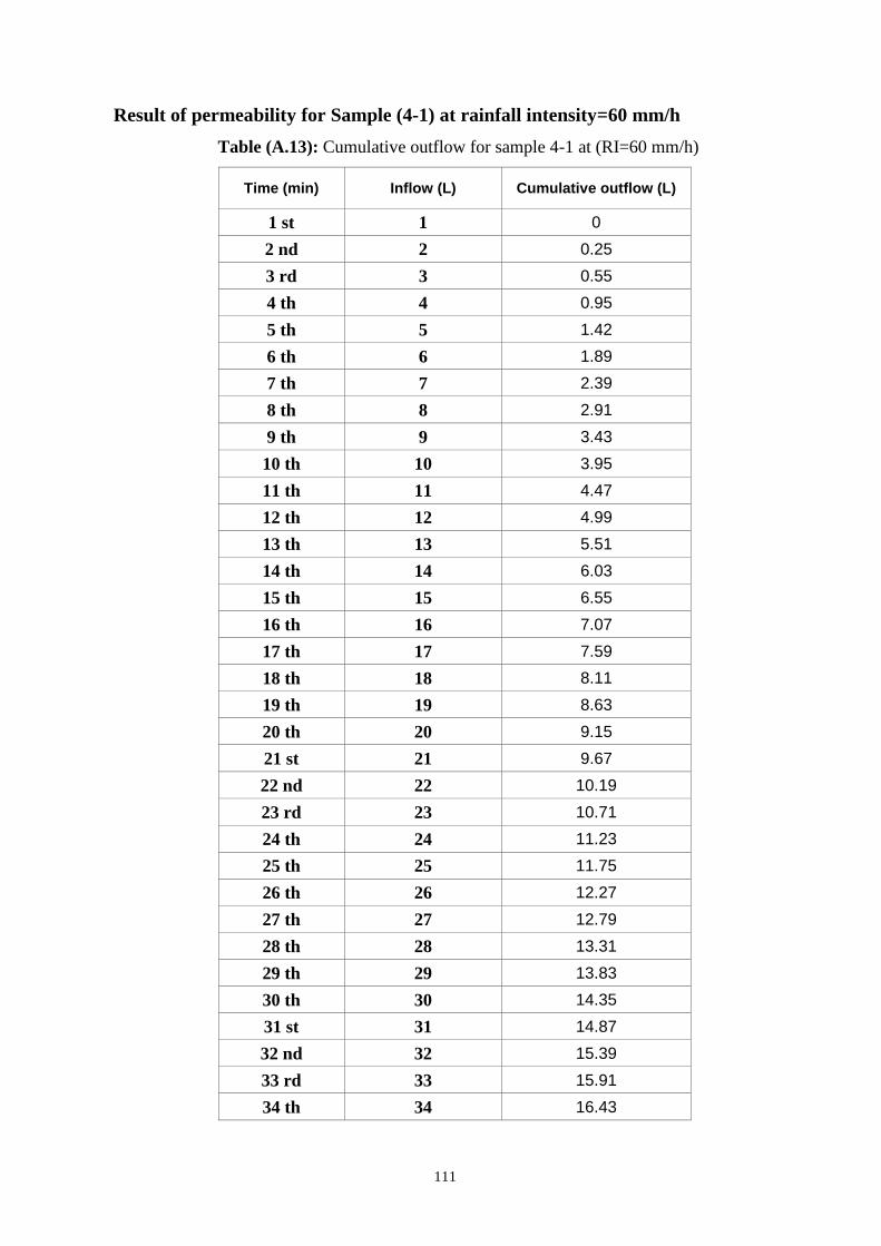
111
Result of permeability for Sample (4-1) at rainfall intensity=60 mm/h
Table (A.13): Cumulative outflow for sample 4-1 at (RI=60 mm/h)
Time (min) Inflow (L) Cumulative outflow (L)
1 st 1 0
2 nd 2 0.25
3 rd 3 0.55
4 th 4 0.95
5 th 5 1.42
6 th 6 1.89
7 th 7 2.39
8 th 8 2.91
9 th 9 3.43
10 th 10 3.95
11 th 11 4.47
12 th 12 4.99
13 th 13 5.51
14 th 14 6.03
15 th 15 6.55
16 th 16 7.07
17 th 17 7.59
18 th 18 8.11
19 th 19 8.63
20 th 20 9.15
21 st 21 9.67
22 nd 22 10.19
23 rd 23 10.71
24 th 24 11.23
25 th 25 11.75
26 th 26 12.27
27 th 27 12.79
28 th 28 13.31
29 th 29 13.83
30 th 30 14.35
31 st 31 14.87
32 nd 32 15.39
33 rd 33 15.91
34 th 34 16.43

112
Time (min) Inflow (L) Cumulative outflow (L)
35 th 35 16.95
36 th 36 17.47
37 th 37 17.99
38 th 38 18.51
39 th 39 19.03
40 th 40 19.55
41 st 41 20.07
42 nd 42 20.59
43 rd 43 21.11
44 th 44 21.63
45 th 45 22.15
46 th 46 22.67
47 th 47 23.19
48 th 48 23.71
49 th 49 24.23
50 th 50 24.75
51 st 51 25.27
52 nd 52 25.79
53 rd 53 26.31
54 th 54 26.83
55 th 55 27.35
56 th 56 27.87
57 th 57 28.39
58 th 58 28.91
59 th 59 29.43
60 th 60 29.95
permeability percentage (%) 49.92

113
Result of permeability for Sample (4-2) at rainfall intensity=60 mm/h
Table (A.14): Cumulative outflow for sample 4-2 at (RI=60 mm/h)
Time (min) Inflow (L) Cumulative outflow (L)
1 st 1 0
2 nd 2 0.25
3 rd 3 0.52
4 th 4 0.84
5 th 5 1.24
6 th 6 1.66
7 th 7 2.13
8 th 8 2.62
9 th 9 3.12
10 th 10 3.62
11 th 11 4.12
12 th 12 4.62
13 th 13 5.12
14 th 14 5.62
15 th 15 6.12
16 th 16 6.62
17 th 17 7.12
18 th 18 7.62
19 th 19 8.12
20 th 20 8.62
21 st 21 9.12
22 nd 22 9.62
23 rd 23 10.12
24 th 24 10.62
25 th 25 11.12
26 th 26 11.62
27 th 27 12.12
28 th 28 12.62
29 th 29 13.12
30 th 30 13.62
31 st 31 14.12
32 nd 32 14.62
33 rd 33 15.12
34 th 34 15.62

114
Time (min) Inflow (L) Cumulative outflow (L)
35 th 35 16.12
36 th 36 16.62
37 th 37 17.12
38 th 38 17.62
39 th 39 18.12
40 th 40 18.62
41 st 41 19.12
42 nd 42 19.62
43 rd 43 20.12
44 th 44 20.62
45 th 45 21.12
46 th 46 21.62
47 th 47 22.12
48 th 48 22.62
49 th 49 23.12
50 th 50 23.62
51 st 51 24.12
52 nd 52 24.62
53 rd 53 25.12
54 th 54 25.62
55 th 55 26.12
56 th 56 26.62
57 th 57 27.12
58 th 58 27.62
59 th 59 28.12
60 th 60 28.62
permeability percentage (%) 47.70

115
Result of permeability for Sample (4-3) at rainfall intensity=60 mm/h
Table (A.15): Cumulative outflow for sample 4-3 at (RI=60 mm/h)
Time (min) Inflow (L) Cumulative outflow (L)
1 st 1 0
2 nd 2 0.23
3 rd 3 0.46
4 th 4 0.73
5 th 5 1.06
6 th 6 1.46
7 th 7 1.9
8 th 8 2.32
9 th 9 2.74
10 th 10 3.19
11 th 11 3.65
12 th 12 4.11
13 th 13 4.57
14 th 14 5.03
15 th 15 5.49
16 th 16 5.95
17 th 17 6.41
18 th 18 6.87
19 th 19 7.33
20 th 20 7.79
21 st 21 8.25
22 nd 22 8.71
23 rd 23 9.17
24 th 24 9.63
25 th 25 10.09
26 th 26 10.55
27 th 27 11.01
28 th 28 11.47
29 th 29 11.93
30 th 30 12.39
31 st 31 12.85
32 nd 32 13.31
33 rd 33 13.77
34 th 34 14.23

116
Time (min) Inflow (L) Cumulative outflow (L)
35 th 35 14.69
36 th 36 15.15
37 th 37 15.61
38 th 38 16.07
39 th 39 16.53
40 th 40 16.99
41 st 41 17.45
42 nd 42 17.91
43 rd 43 18.37
44 th 44 18.83
45 th 45 19.29
46 th 46 19.75
47 th 47 20.21
48 th 48 20.67
49 th 49 21.13
50 th 50 21.59
51 st 51 22.05
52 nd 52 22.51
53 rd 53 22.97
54 th 54 23.43
55 th 55 23.89
56 th 56 24.35
57 th 57 24.81
58 th 58 25.27
59 th 59 25.73
60 th 60 26.19
permeability percentage (%) 43.65

117
Result of permeability for Sample (4-4) at rainfall intensity=60 mm/h
Table (A.16): Cumulative outflow for sample 4-4 at (RI=60 mm/h)
Time (min) Inflow (L) Cumulative outflow (L)
1 st 1 0
2 nd 2 0.21
3 rd 3 0.43
4 th 4 0.64
5 th 5 0.97
6 th 6 1.38
7 th 7 1.8
8 th 8 2.22
9 th 9 2.66
10 th 10 3.1
11 th 11 3.55
12 th 12 3.99
13 th 13 4.43
14 th 14 4.87
15 th 15 5.31
16 th 16 5.75
17 th 17 6.19
18 th 18 6.63
19 th 19 7.07
20 th 20 7.51
21 st 21 7.95
22 nd 22 8.39
23 rd 23 8.83
24 th 24 9.27
25 th 25 9.71
26 th 26 10.15
27 th 27 10.59
28 th 28 11.03
29 th 29 11.47
30 th 30 11.91
31 st 31 12.35
32 nd 32 12.79
33 rd 33 13.23
34 th 34 13.67

118
35 th 35 14.11
36 th 36 14.55
37 th 37 14.99
38 th 38 15.43
39 th 39 15.87
40 th 40 16.31
41 st 41 16.75
42 nd 42 17.19
43 rd 43 17.63
44 th 44 18.07
45 th 45 18.51
46 th 46 18.95
47 th 47 19.39
48 th 48 19.83
49 th 49 20.27
50 th 50 20.71
51 st 51 21.15
52 nd 52 21.59
53 rd 53 22.03
54 th 54 22.47
55 th 55 22.91
56 th 56 23.35
57 th 57 23.79
58 th 58 24.23
59 th 59 24.67
60 th 60 25.11
permeability percentage (%) 41.85

119
Appendix (B)
Interlock Tile Tests

120
Result of Compressive Strength and Absorption for Sample (1-1)
Table (B.1): Compressive Strength &Absorption for sample 1-1
Specimen No.
Dimensions (cm) Chamfer Factor
Weight Fracture
Load (KN)
Stress Density (kg/m3)
Area (cm2)
thickness (cm)
g Kg/cm2
1 200.0 8.00 1.18 3130.0 734.7 441.9 1956.3
2 200.0 8.00 1.18 2930.0 502.6 302.3 1831.3
3 200.0 8.00 1.18 3060.0 601.0 361.5 1912.5
4 200.0 8.00 1.18 3255.0 816.9 491.3 2034.4
5 200.0 8.00 1.18 2568.0 487.1 293.0 1605.0
6 200.0 8.00 1.18 3160.0 518.6 311.9 1975.0
7 200.0 8.00 1.18 2990.0 572.4 344.3 1868.8
8 200.0 8.00 1.18 3140.0 608.0 365.7 1962.5
9 200.0 8.00 1.18 2895.0 635.5 382.2 1809.4
10 200.0 8.00 1.18 3195.0 670.6 403.3 1996.9
Average Stress 370 Kg/cm2
Standard Deviation 63.1 Kg/cm2
Variation 53.6 %
Specimen No. Dimensions (cm) Dry
weight (g)
After 24 hours
Area (cm2) thickness
(cm)
wet Weight
(g)
Absorption %
1 200.0 8.0 3080.0 3170.0 2.9
2 200.0 8.0 3025.0 3105.0 2.6
3 200.0 8.0 3095.0 3170.0 2.4
4 200.0 8.0 2775.0 2830.0 2.0
5 200.0 8.0 3060.0 3150.0 2.9
6 200.0 8.0 3225.0 3305.0 2.5
7 200.0 8.0 2910.0 2980.0 2.4
8 200.0 8.0 2905.0 2970.0 2.2
9 200.0 8.0 2890.0 2950.0 2.1
10 200.0 8.0 3270.0 3350.0 2.4
24 hours
Average Absorption 2.46 %
Standard Deviation 0.32 %

121
Result of Compressive Strength and Absorption for Sample (1-2)
Table (B.2): Compressive Strength &Absorption for sample 1-2
Specimen No. Dimensions (cm) Weight
Fracture Load (KN)
Density (kg/m3)
Compressive
Strength Kg/cm2
Area (cm2)
Thickness (cm)
g
1 200.0 8.0 3090.0 710.2 1931 427.1
2 200.0 8.0 2870.0 475.6 1794 286.0
3 200.0 8.0 3077.0 550.0 1923 330.8
4 200.0 8.0 3145.0 760.0 1966 457.1
5 200.0 8.0 2458.0 460.0 1536 276.7
6 200.0 8.0 3060.0 490.6 1913 295.1
7 200.0 8.0 2750.0 542.7 1719 326.4
8 200.0 8.0 2540.0 505.0 1588 303.7
9 200.0 8.0 2655.0 525.5 1659 316.0
10 200.0 8.0 3095.0 565.0 1934 339.8
Average Stress 336 Kg/cm2
Standard Deviation 59.8 Kg/cm2
Variation
53.7 %
Specimen No. Dimensions (cm)
Dry weight
(g)
After 24 hours
Area (cm2) thickness
(cm)
wet Weight
(g)
Absorption %
1 200.0 8.0 3075.0 3160.0 2.8
2 200.0 8.0 3015.0 3085.0 2.3
3 200.0 8.0 2930.0 2995.0 2.2
4 200.0 8.0 2875.0 2950.0 2.6
5 200.0 8.0 3010.0 3085.0 2.5
6 200.0 8.0 3115.0 3200.0 2.7
7 200.0 8.0 2815.0 2890.0 2.7
8 200.0 8.0 2815.0 2880.0 2.3
9 200.0 8.0 2790.0 2860.0 2.5
10 200.0 8.0 3270.0 3035.0 2.2
24 hours
Average Absorption 2.48 %
Standard Deviation 0.21 %

122
Result of Compressive Strength and Absorption for Sample (1-3)
Table (B.3): Compressive Strength &Absorption for sample 1-3 Specimen No. Dimensions (cm) Weight
Fracture Load (KN)
Density (kg/m3)
Compressive
Strength Kg/cm2
Area (cm2)
Thickness (cm)
g
1 200.0 8.0 3065.0 545.2 1916 327.9
2 200.0 8.0 2955.0 516.0 1847 310.3
3 200.0 8.0 2725.0 476.2 1703 286.4
4 200.0 8.0 3215.0 578.0 2009 347.6
5 200.0 8.0 3136.0 600.1 1960 360.9
6 200.0 8.0 3205.0 625.0 2003 375.9
7 200.0 8.0 2760.0 438.3 1725 263.6
8 200.0 8.0 2975.0 512.0 1859 307.9
9 200.0 8.0 2615.0 416.2 1634 250.3
10 200.0 8.0 2840.0 487.5 1775 293.2
Average Stress 312 Kg/cm2
Standard Deviation 41.1 Kg/cm2
Variation 40.2 %
Specimen No. Dimensions (cm)
Dry weight
(g)
After 24 hours
Area (cm2) thickness
(cm)
wet Weight
(g)
Absorption %
1 200.0 8.0 2995.0 3070.0 2.5
2 200.0 8.0 3080.0 3165.0 2.8
3 200.0 8.0 3105.0 3190.0 2.7
4 200.0 8.0 3055.0 3125.0 2.3
5 200.0 8.0 2895.0 2975.0 2.8
6 200.0 8.0 2910.0 3015.0 3.6
7 200.0 8.0 3205.0 3280.0 2.3
8 200.0 8.0 3125.0 3195.0 2.2
9 200.0 8.0 3095.0 3165.0 2.3
10 200.0 8.0 3145.0 3215.0 2.2
24 hours
Average Absorption 2.57 %
Standard Deviation 0.43 %

123
Result of Compressive Strength and Absorption for Sample (1-4)
Table (B.4): Compressive Strength &Absorption for sample 1-4 Specimen No. Dimensions (cm) Weight
Fracture Load (KN)
Density (kg/m3)
Compressive
Strength Kg/cm2
Area (cm2)
Thickness (cm)
g
1 200.0 8.0 2975.0 445.4 1859 267.9
2 200.0 8.0 2915.0 496.0 1822 298.3
3 200.0 8.0 2775.0 418.3 1734 251.6
4 200.0 8.0 3105.0 485.0 1941 291.7
5 200.0 8.0 2865.0 464.0 1791 279.1
6 200.0 8.0 3245.0 502.1 2028 302.0
7 200.0 8.0 3115.0 488.0 1947 293.5
8 200.0 8.0 2975.0 493.2 1859 296.6
9 200.0 8.0 2925.0 500.0 1828 300.7
10 200.0 8.0 2875.0 467.5 1797 281.2
Average Stress 286 Kg/cm2
Standard Deviation 16.4 Kg/cm2
Variation 17.6 %
Specimen No. Dimensions (cm)
Dry weight
(g)
After 24 hours
Area (cm2) thickness
(cm)
wet Weight
(g)
Absorption %
1 200.0 8.0 3115.0 3190.0 2.4
2 200.0 8.0 2765.0 2845.0 2.9
3 200.0 8.0 2790.0 2865.0 2.7
4 200.0 8.0 3215.0 3300.0 2.6
5 200.0 8.0 3220.0 3315.0 3.0
6 200.0 8.0 2955.0 3035.0 2.7
7 200.0 8.0 3205.0 3280.0 2.3
8 200.0 8.0 3250.0 3365.0 3.5
9 200.0 8.0 3095.0 3180.0 2.7
10 200.0 8.0 3120.0 3195.0 2.4
24 hours
Average Absorption 2.73 %
Standard Deviation 0.35 %

124
Result of Compressive Strength and Absorption for Sample (2-1)
Table (B.5): Compressive Strength &Absorption for sample 2-1
Specimen No. Dimensions (cm) Weight
Fracture Load (KN)
Density (kg/m3)
Compressive
Strength Kg/cm2
Area (cm2)
Thickness (cm)
g
1 200.0 8.0 3020.0 375.6 1888 225.9
2 200.0 8.0 3115.0 491.6 1947 295.7
3 200.0 8.0 3075.0 376.2 1922 226.3
4 200.0 8.0 3090.0 461.4 1931 277.5
5 200.0 8.0 3060.0 539.8 1913 324.7
6 200.0 8.0 3110.0 375.7 1944 226.0
7 200.0 8.0 3175.0 478.6 1984 287.8
8 200.0 8.0 3165.0 390.2 1978 234.7
9 200.0 8.0 3040.0 553.1 1900 332.6
10 200.0 8.0 3180.0 556.8 1988 334.9
Average Stress 277 Kg/cm2
Standard Deviation 45.7 Kg/cm2
Variation 39.4 %
Specimen No. Dimensions (cm)
Dry weight
(g)
After 24 hours
Area (cm2) thickness
(cm)
wet Weight
(g)
Absorption %
1 200.0 8.0 3075.0 3175.0 3.3
2 200.0 8.0 3140.0 3230.0 2.9
3 200.0 8.0 2985.0 3060.0 2.5
4 200.0 8.0 3110.0 3195.0 2.7
5 200.0 8.0 3055.0 3135.0 2.6
6 200.0 8.0 3115.0 3205.0 2.9
7 200.0 8.0 2940.0 3020.0 2.7
8 200.0 8.0 3185.0 3270.0 2.7
9 200.0 8.0 3030.0 3110.0 2.6
10 200.0 8.0 2865.0 2925.0 2.9
24 hours
Average Absorption 2.78 %
Standard Deviation 0.21 %

125
Result of Compressive Strength and Absorption for Sample (2-2)
Table (B.6): Compressive Strength &Absorption for sample 2-2 Specimen No. Dimensions (cm) Weight
Fracture Load (KN)
Density (kg/m3)
Compressive
Strength Kg/cm2
Area (cm2)
Thickness (cm)
g
1 200.0 8.0 3130.0 445.5 1956 267.9
2 200.0 8.0 3085.0 385.6 1928 231.9
3 200.0 8.0 3175.0 528.2 1984 317.7
4 200.0 8.0 3105.0 471.2 1941 283.4
5 200.0 8.0 3125.0 529.4 1953 318.4
6 200.0 8.0 3215.0 515.5 2009 310.0
7 200.0 8.0 2875.0 408.6 1797 245.7
8 200.0 8.0 3015.0 493.1 1884 296.6
9 200.0 8.0 3170.0 583.5 1981 350.9
10 200.0 8.0 3095.0 578.3 1934 347.8
Average Stress 297 Kg/cm2
Standard Deviation 40.1 Kg/cm2
Variation 40.1 %
Specimen No. Dimensions (cm) Dry weight
(g)
After 24 hours
Area (cm2)
thickness (cm)
wet Weight (g)
Absorption %
1 200.0 8.0 3015.0 3115.0 3.3
2 200.0 8.0 3035.0 3115.0 2.6
3 200.0 8.0 3125.0 3210.0 2.7
4 200.0 8.0 3085.0 3165.0 2.6
5 200.0 8.0 2895.0 2965.0 2.4
6 200.0 8.0 2995.0 3075.0 2.7
7 200.0 8.0 3005.0 3095.0 3.0
8 200.0 8.0 3045.0 3125.0 2.6
9 200.0 8.0 3205.0 3275.0 2.2
10 200.0 8.0 3110.0 3185.0 2.4
24 hours
Average Absorption 2.66 %
Standard Deviation 0.32 %

126
Result of Compressive Strength and Absorption for Sample (2-3)
Table (B.7): Compressive Strength &Absorption for sample 2-3
Specimen No. Dimensions (cm) Weight
Fracture Load (KN)
Density (kg/m3)
Compressive Strength Kg/cm2
Area (cm2)
Thickness (cm)
g
1 200.0 8.0 3060.0 378.5 1913 227.6
2 200.0 8.0 3110.0 388.7 1944 233.8
3 200.0 8.0 3105.0 375.5 1941 225.8
4 200.0 8.0 2910.0 349.2 1819 210.0
5 200.0 8.0 2965.0 358.0 1853 215.3
6 200.0 8.0 3160.0 436.3 1975 262.4
7 200.0 8.0 3095.0 334.2 1934 201.0
8 200.0 8.0 3205.0 375.5 2003 225.8
9 200.0 8.0 3085.0 345.5 1928 207.8
10 200.0 8.0 3175.0 472.3 1984 284.1
Average Stress 229 Kg/cm2
Standard Deviation 25.8 Kg/cm2
Variation 36.2 %
Specimen No. Dimensions (cm) Dry weight
(g)
After 24 hours
Area (cm2)
thickness (cm)
wet Weight (g)
Absorption %
1 200.0 8.0 2885.0 2990.0 3.6
2 200.0 8.0 2870.0 2975.0 3.7
3 200.0 8.0 3065.0 3165.0 3.3
4 200.0 8.0 3120.0 3235.0 3.7
5 200.0 8.0 3160.0 3245.0 2.7
6 200.0 8.0 3105.0 3195.0 2.9
7 200.0 8.0 3185.0 3300.0 3.6
8 200.0 8.0 3075.0 3185.0 3.6
9 200.0 8.0 2795.0 2900.0 3.8
10 200.0 8.0 2965.0 3050.0 2.9
24 hours
Average Absorption 3.36 %
Standard Deviation 0.40 %

127
Result of Compressive Strength and Absorption for Sample (2-4)
Table (B.8): Compressive Strength &Absorption for sample 2-4
Specimen No. Dimensions (cm) Chamfer Factor
Weight Fracture
Load (KN)
Stress Density (kg/m3)
Area (cm2) thickness
(cm) g Kg/cm2
1 200.0 8.00 1.18 3020.0 342.6 206.0 1887.5
2 200.0 8.00 1.18 3215.0 418.2 251.5 2009.4
3 200.0 8.00 1.18 3230.0 475.0 285.7 2018.8
4 200.0 8.00 1.18 3205.0 456.2 274.4 2003.1
5 200.0 8.00 1.18 2995.0 362.3 217.9 1871.9
6 200.0 8.00 1.18 2905.0 384.0 230.9 1815.6
7 200.0 8.00 1.18 3310.0 547.2 329.1 2068.8
8 200.0 8.00 1.18 3175.0 345.5 207.8 1984.4
9 200.0 8.00 1.18 3030.0 367.1 220.8 1893.8
10 200.0 8.00 1.18 2860.0 398.0 239.4 1787.5
Average Stress 246 Kg/cm2
Standard Deviation 39.5 Kg/cm2
Variation 49.9 %
Specimen No. Dimensions (cm) Dry weight
(g)
After 24 hours
Area (cm2)
thickness (cm)
wet Weight (g)
Absorption %
1 200.0 8.0 2780.0 2865.0 3.1
2 200.0 8.0 2925.0 3005.0 2.7
3 200.0 8.0 3030.0 3135.0 3.5
4 200.0 8.0 3095.0 3205.0 3.6
5 200.0 8.0 2985.0 3075.0 3.0
6 200.0 8.0 2910.0 2985.0 2.6
7 200.0 8.0 3120.0 3215.0 3.0
8 200.0 8.0 3175.0 3290.0 3.6
9 200.0 8.0 3065.0 3165.0 3.3
10 200.0 8.0 3090.0 3180.0 2.9
24 hours
Average Absorption 3.12 %
Standard Deviation 0.35 %

128
Result of Compressive Strength and Absorption for Sample (3-1)
Table (B.9): Compressive Strength &Absorption for sample 3-1 Specimen No. Dimensions (cm) Weight
Fracture Load (KN)
Density (kg/m3)
Compressive Strength Kg/cm2
Area (cm2)
Thickness (cm)
G
1 200.0 8.0 2780.0 400.8 1738 241.1
2 200.0 8.0 2840.0 400.2 1775 240.7
3 200.0 8.0 3105.0 738.4 1941 444.1
4 200.0 8.0 2960.0 491.5 1850 295.6
5 200.0 8.0 2875.0 452.2 1797 272.0
6 200.0 8.0 2805.0 477.1 1753 286.9
7 200.0 8.0 2885.0 464.4 1803 279.3
8 200.0 8.0 3065.0 699.2 1916 420.5
9 200.0 8.0 2930.0 462.4 1831 278.1
10 200.0 8.0 3020.0 662.9 1888 398.7
Average Stress 316 Kg/cm2
Standard Deviation 75.6 Kg/cm2
Variation 64.4 %
Specimen No. Dimensions (cm) Dry weight
(g)
After 24 hours
Area (cm2)
thickness (cm)
wet Weight (g)
Absorption %
1 200.0 8.0 3055.0 3135.0 2.6
2 200.0 8.0 2835.0 2900.0 2.3
3 200.0 8.0 2905.0 2980.0 2.6
4 200.0 8.0 3000.0 3080.0 2.7
5 200.0 8.0 2930.0 3015.0 2.9
6 200.0 8.0 3005.0 3085.0 2.7
7 200.0 8.0 2765.0 2840.0 2.7
8 200.0 8.0 2780.0 2845.0 2.3
9 200.0 8.0 2865.0 2925.0 2.2
10 200.0 8.0 3270.0 3350.0 2.5
24 hours
Average Absorption 2.55 %
Standard Deviation 0.21 %

129
Result of Compressive Strength and Absorption for Sample (3-2)
Table (B.10): Compressive Strength &Absorption for sample 3-2 Specimen No. Dimensions (cm) Weight
Fracture Load (KN)
Density (kg/m3)
Compressive Strength Kg/cm2
Area (cm2)
Thickness (cm)
g
1 200.0 8.0 2845.0 518.2 1778 311.7
2 200.0 8.0 2805.0 456.0 1753 274.3
3 200.0 8.0 2665.0 398.5 1666 239.7
4 200.0 8.0 2795.0 467.1 1747 280.9
5 200.0 8.0 3010.0 532.4 1881 320.2
6 200.0 8.0 2925.0 557.1 1828 335.1
7 200.0 8.0 3060.0 561.5 1913 337.7
8 200.0 8.0 3145.0 573.0 1966 344.6
9 200.0 8.0 2670.0 477.1 1669 286.9
10 200.0 8.0 2635.0 462.9 1647 278.4
Average Stress 301 Kg/cm2
Standard Deviation 34.1 Kg/cm2
Variation 34.9 %
Specimen No. Dimensions (cm) Dry weight
(g)
After 24 hours
Area (cm2)
thickness (cm)
wet Weight (g)
Absorption %
1 200.0 8.0 3015.0 3085.0 2.3
2 200.0 8.0 2685.0 2765.0 3.0
3 200.0 8.0 2730.0 2800.0 2.6
4 200.0 8.0 2760.0 2835.0 2.7
5 200.0 8.0 2825.0 2905.0 2.8
6 200.0 8.0 3100.0 3185.0 2.7
7 200.0 8.0 2575.0 2635.0 2.3
8 200.0 8.0 2660.0 2730.0 2.6
9 200.0 8.0 2865.0 2925.0 2.4
10 200.0 8.0 2890.0 2960.0 2.4
24 hours
Average Absorption 2.60 %
Standard Deviation 0.22 %

130
Result of Compressive Strength and Absorption for Sample (3-3)
Table (B.11): Compressive Strength &Absorption for sample 3-3 Specimen No. Dimensions (cm)
Chamfer Factor
Weight Fracture
Load (KN)
Stress Density (kg/m3)
Area (cm2) thickness
(cm) g Kg/cm2
1 200.0 8.00 1.18 3020.0 526.1 316.4 1887.5
2 200.0 8.00 1.18 3075.0 566.7 340.8 1921.9
3 200.0 8.00 1.18 2765.0 545.5 328.1 1728.1
4 200.0 8.00 1.18 2915.0 572.0 344.0 1821.9
5 200.0 8.00 1.18 2890.0 587.4 353.3 1806.3
6 200.0 8.00 1.18 2775.0 456.3 274.4 1734.4
7 200.0 8.00 1.18 2780.0 480.0 288.7 1737.5
8 200.0 8.00 1.18 3125.0 688.1 413.8 1953.1
9 200.0 8.00 1.18 3145.0 561.5 337.7 1965.6
10 200.0 8.00 1.18 2955.0 590.5 355.1 1846.9
Average Stress 335 Kg/cm2
Standard Deviation 38.4 Kg/cm2
Variation 41.6 %
Specimen No. Dimensions (cm) Dry weight
(g)
After 24 hours
Area (cm2)
thickness (cm)
wet Weight (g)
Absorption %
1 200.0 8.0 2670.0 2745.0 2.8
2 200.0 8.0 2645.0 2715.0 2.6
3 200.0 8.0 2585.0 2645.0 2.3
4 200.0 8.0 2730.0 2800.0 2.6
5 200.0 8.0 2815.0 2880.0 2.3
6 200.0 8.0 3040.0 3120.0 2.6
7 200.0 8.0 2975.0 3050.0 2.5
8 200.0 8.0 2880.0 2945.0 2.3
9 200.0 8.0 2865.0 2925.0 2.7
10 200.0 8.0 2590.0 2645.0 2.1
24 hours
Average Absorption 2.49 %
Standard Deviation 0.22 %

131
Result of Compressive Strength and Absorption for Sample (3-4)
Table (B.12): Compressive Strength &Absorption for sample 3-4 Specimen No. Dimensions (cm) Weight
Fracture Load (KN)
Density (kg/m3)
Compressive Strength Kg/cm2
Area (cm2)
Thickness (cm)
G
1 200.0 8.0 3100.0 554.2 1938 333.3
2 200.0 8.0 2595.0 389.2 1622 234.1
3 200.0 8.0 2825.0 473.0 1766 284.5
4 200.0 8.0 2865.0 574.0 1791 345.2
5 200.0 8.0 2685.0 495.5 1678 298.0
6 200.0 8.0 3060.0 547.2 1913 329.1
7 200.0 8.0 3205.0 623.1 2003 374.7
8 200.0 8.0 2945.0 537.7 1841 323.4
9 200.0 8.0 2680.0 502.1 1675 302.0
10 200.0 8.0 2975.0 618.6 1859 372.0
Average Stress 320 Kg/cm2
Standard Deviation 42.3 Kg/cm2
Variation 44.0 %
Specimen No. Dimensions (cm) Dry weight
(g)
After 24 hours
Area (cm2)
thickness (cm)
wet Weight (g)
Absorption %
1 200.0 8.0 3115.0 3200.0 2.7
2 200.0 8.0 3065.0 3135.0 2.3
3 200.0 8.0 2935.0 3015.0 2.7
4 200.0 8.0 2755.0 2825.0 2.5
5 200.0 8.0 2785.0 2850.0 2.3
6 200.0 8.0 2810.0 2880.0 2.5
7 200.0 8.0 2690.0 2755.0 2.4
8 200.0 8.0 2605.0 2675.0 2.7
9 200.0 8.0 2865.0 2925.0 2.6
10 200.0 8.0 2995.0 3065.0 2.3
24 hours
Average Absorption 2.52 %
Standard Deviation 0.17 %

132
Result of Compressive Strength and Absorption for Sample (4-1)
Table (B.13): Compressive Strength &Absorption for sample 4-1 Specimen No. Dimensions (cm) Weight
Fracture Load (KN)
Density (kg/m3)
Compressive Strength Kg/cm2
Area (cm2)
Thickness (cm)
g
1 200.0 8.0 2740.0 308.4 1713 185.5
2 200.0 8.0 2735.0 317.8 1709 191.1
3 200.0 8.0 2780.0 396.7 1738 238.6
4 200.0 8.0 2700.0 557.5 1688 335.3
5 200.0 8.0 3065.0 374.8 1916 225.4
6 200.0 8.0 2725.0 378.1 1703 227.4
7 200.0 8.0 2745.0 391.7 1716 235.6
8 200.0 8.0 2870.0 327.3 1794 196.8
9 200.0 8.0 2850.0 360.5 1781 216.8
10 200.0 8.0 2885.0 425.2 1803 255.7
Average Stress 231 Kg/cm2
Standard Deviation 43.0 Kg/cm2
Variation 64.9 %
Specimen No. Dimensions (cm) Dry
weight (g)
After 24 hours
Area (cm2) thickness
(cm)
wet Weight
(g)
Absorption %
1 200.0 8.0 2720.0 2815.0 3.5
2 200.0 8.0 2950.0 3045.0 3.2
3 200.0 8.0 2840.0 2955.0 4.0
4 200.0 8.0 2675.0 2760.0 3.2
5 200.0 8.0 2780.0 2870.0 3.2
6 200.0 8.0 2945.0 3040.0 3.2
7 200.0 8.0 2805.0 2885.0 2.9
8 200.0 8.0 2690.0 2775.0 3.2
9 200.0 8.0 2705.0 2800.0 3.5
10 200.0 8.0 2865.0 2925.0 2.9
24 hours
Average Absorption 3.28 %
Standard Deviation 0.34 %

133
Result of Compressive Strength and Absorption for Sample (4-2)
Table (B.14): Compressive Strength &Absorption for sample 4-2 Specimen No. Dimensions (cm)
Chamfer Factor
Weight Fracture
Load (KN)
Stress Density (kg/m3)
Area (cm2) thickness
(cm) g Kg/cm2
1 200.0 8.00 1.18 2695.0 317.4 190.9 1684.4
2 200.0 8.00 1.18 2755.0 345.6 207.9 1721.9
3 200.0 8.00 1.18 2835.0 427.1 256.9 1771.9
4 200.0 8.00 1.18 3070.0 477.5 287.2 1918.8
5 200.0 8.00 1.18 2840.0 385.2 231.7 1775.0
6 200.0 8.00 1.18 2825.0 391.5 235.5 1765.6
7 200.0 8.00 1.18 2890.0 399.2 240.1 1806.3
8 200.0 8.00 1.18 2830.0 418.4 251.6 1768.8
9 200.0 8.00 1.18 2975.0 483.0 290.5 1859.4
10 200.0 8.00 1.18 2860.0 498.2 299.6 1787.5
Average Stress 249 Kg/cm2
Standard Deviation 35.7 Kg/cm2
Variation 43.6 %
Specimen No. Dimensions (cm) Dry
weight (g)
After 24 hours
Area (cm2) thickness
(cm)
wet Weight
(g)
Absorption %
1 200.0 8.0 3020.0 3105.0 2.8
2 200.0 8.0 2970.0 3065.0 3.2
3 200.0 8.0 2685.0 2745.0 2.2
4 200.0 8.0 2775.0 2865.0 3.2
5 200.0 8.0 2740.0 2815.0 2.7
6 200.0 8.0 2830.0 2915.0 3.0
7 200.0 8.0 2650.0 2725.0 2.8
8 200.0 8.0 2975.0 3075.0 3.4
9 200.0 8.0 2725.0 2800.0 2.8
10 200.0 8.0 2780.0 2860.0 2.9
24 hours
Average Absorption 2.91 %
Standard Deviation 0.32 %

134
Result of Compressive Strength and Absorption for Sample (4-3)
Table (B.15): Compressive Strength &Absorption for sample 4-3 Specimen No. Dimensions (cm) Weight
Fracture Load (KN)
Density (kg/m3)
Compressive Strength Kg/cm2
Area (cm2)
Thickness (cm)
g
1 200.0 8.0 3050.0 439.2 1906 264.1
2 200.0 8.0 3125.0 533.0 1953 320.6
3 200.0 8.0 2775.0 368.3 1734 221.5
4 200.0 8.0 2830.0 365.1 1769 219.6
5 200.0 8.0 2815.0 379.0 1759 227.9
6 200.0 8.0 2905.0 388.5 1816 233.7
7 200.0 8.0 2675.0 372.7 1672 224.2
8 200.0 8.0 2980.0 436.3 1863 262.4
9 200.0 8.0 2765.0 398.2 1728 239.5
10 200.0 8.0 2845.0 512.5 1778 308.2
Average Stress 252 Kg/cm2
Standard Deviation 36.4 Kg/cm2
Variation 40.0 %
Specimen No. Dimensions (cm) Dry
weight (g)
After 24 hours
Area (cm2) thickness
(cm)
wet Weight
(g)
Absorption %
1 200.0 8.0 2860.0 2935.0 2.6
2 200.0 8.0 2835.0 2930.0 3.4
3 200.0 8.0 2785.0 2855.0 2.5
4 200.0 8.0 2690.0 2765.0 2.8
5 200.0 8.0 2675.0 2775.0 3.7
6 200.0 8.0 2910.0 2985.0 2.6
7 200.0 8.0 2760.0 2830.0 2.5
8 200.0 8.0 2815.0 2895.0 2.8
9 200.0 8.0 2905.0 2985.0 2.8
10 200.0 8.0 2720.0 2805.0 3.1
24 hours
Average Absorption 2.88 %
Standard Deviation 0.40 %
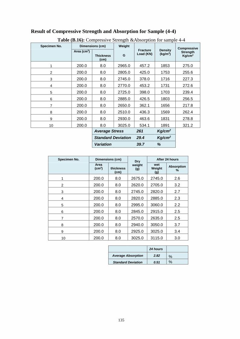
135
Result of Compressive Strength and Absorption for Sample (4-4)
Table (B.16): Compressive Strength &Absorption for sample 4-4 Specimen No. Dimensions (cm) Weight
Fracture Load (KN)
Density (kg/m3)
Compressive Strength Kg/cm2
Area (cm2)
Thickness (cm)
G
1 200.0 8.0 2965.0 457.2 1853 275.0
2 200.0 8.0 2805.0 425.0 1753 255.6
3 200.0 8.0 2745.0 378.0 1716 227.3
4 200.0 8.0 2770.0 453.2 1731 272.6
5 200.0 8.0 2725.0 398.0 1703 239.4
6 200.0 8.0 2885.0 426.5 1803 256.5
7 200.0 8.0 2650.0 362.1 1656 217.8
8 200.0 8.0 2510.0 436.3 1569 262.4
9 200.0 8.0 2930.0 463.6 1831 278.8
10 200.0 8.0 3025.0 534.1 1891 321.2
Average Stress 261 Kg/cm2
Standard Deviation 29.4 Kg/cm2
Variation 39.7 %
Specimen No. Dimensions (cm) Dry
weight (g)
After 24 hours
Area (cm2) thickness
(cm)
wet Weight
(g)
Absorption %
1 200.0 8.0 2675.0 2745.0 2.6
2 200.0 8.0 2620.0 2705.0 3.2
3 200.0 8.0 2745.0 2820.0 2.7
4 200.0 8.0 2820.0 2885.0 2.3
5 200.0 8.0 2995.0 3060.0 2.2
6 200.0 8.0 2845.0 2915.0 2.5
7 200.0 8.0 2570.0 2635.0 2.5
8 200.0 8.0 2940.0 3050.0 3.7
9 200.0 8.0 2925.0 3025.0 3.4
10 200.0 8.0 3025.0 3115.0 3.0
24 hours
Average Absorption 2.82 %
Standard Deviation 0.51 %

136
Appendix (C)
Aggregate Tests

137
Result of Folia Aggregate Sieve Analyses
0.00
10.00
20.00
30.00
40.00
50.00
60.00
70.00
80.00
90.00
100.00
0.01 0.10 1.00 10.00 100.00
% P
assin
g
Sieve Size (mm)
Medium Aggregate I –
Folia
G 2154 Dry Wt. Before Sieving:
% Passing Cumulative % Retained
% Retained Weight Retained
(gm)
Sieve Opening
Size (mm)
Sieve No.
100.00 0.0 0.00 0.0 25.00 1"
94.73 5.3 5.27 113.5 19.00 3/4"
9.40 90.6 85.33 1838.0 12.50 1/2"
3.90 96.1 5.50 118.5 9.50 3/8"
2.53 97.5 1.37 29.5 4.75 #4
2.53 97.5 0.00 0.0 2.36 #8
2.53 97.5 0.00 0.0 1.180 #16
2.53 97.5 0.00 0.0 0.600 #30
2.53 97.5 0.00 0.0 0.300 #50
2.53 97.5 0.00 0.0 0.150 #100
2.53 97.5 0.00 0.0 0.075 #200
0.00 100.0 2.53 54.5 0.000 Pan

138
Result of Adasia Aggregate Sieve Analyses
Medium Aggregate II
- Adasia
g 2656 Dry Wt. Before
Sieving: % Passing Cumulative %
Retained % Retained Weight
Retained (gm)
Sieve Opening
Size (mm)
Sieve No.
100.00 0.0 0.00 0.0 25.00 1"
100.00 0.0 0.00 0.0 19.00 3/4"
68.75 31.3 31.25 830.0 12.50 1/2"
19.94 80.1 48.81 1296.5 9.50 3/8"
0.36 99.6 19.58 520.0 4.75 #4
0.26 99.7 0.09 2.5 2.36 #8
0.13 99.9 0.13 3.5 1.180 #16
0.06 99.9 0.08 2.0 0.600 #30
0.00 100.0 0.06 1.5 0.300 #50
0.00 100.0 0.00 0.0 0.150 #100
0.00 100.0 0.00 0.0 0.075 #200
0.00 100.0 0.00 0.0 0.000 pan
0.00
10.00
20.00
30.00
40.00
50.00
60.00
70.00
80.00
90.00
100.00
0.10 1.00 10.00 100.00
% P
assin
g
Sieve Size (mm)

139
Result of Semsemia Aggregate Sieve Analyses
Medium Aggregate III -
Semsemia
g 2076 Dry Wt. Before Sieving: % Passing Cumulative %
Retained % Retained Weight
Retained (gm)
Sieve Opening
Size (mm)
Sieve No.
100.00 0.0 0.00 0.0 25.00 1"
100.00 0.0 0.00 0.0 19.00 3/4"
100.00 0.0 0.00 0.0 12.50 1/2"
98.34 1.7 1.66 34.5 9.50 3/8"
22.28 77.7 76.06 1579.0 4.75 #4
5.06 94.9 17.22 357.5 2.36 #8
2.22 97.8 2.84 59.0 1.180 #16
1.32 98.7 0.89 18.5 0.600 #30
1.08 98.9 0.24 5.0 0.300 #50
0.96 99.0 0.12 2.5 0.150 #100
0.94 99.1 0.02 0.5 0.075 #200
0.00 100.0 0.94 19.5 0.000 pan
0.00
10.00
20.00
30.00
40.00
50.00
60.00
70.00
80.00
90.00
100.00
0.10 1.00 10.00 100.00
% P
assin
g
Sieve Size (mm)

140
Result of Sand Aggregate Sieve Analyses
Sand
g 1954 Dry Wt. Before
Sieving: % Passing Cumulative %
Retained % Retained Weight
Retained (gm)
Sieve Opening
Size (mm)
Sieve No.
100.00 0.0 0.0 0.0 25.00 1"
100.00 0.0 0.0 0.0 19.00 3/4"
100.00 0.0 0.0 0.0 12.50 1/2"
100.00 0.0 0.0 0.0 9.50 3/8"
100.00 0.0 0.0 0.0 4.75 #4
100.00 0.0 0.0 0.0 2.36 #8
99.9 0.1 0.10 1.9 1.180 #16
99.6 0.4 0.3 5.86 0.600 #30
93.7 6.3 5.9 115.3 0.300 #50
2 98 91.7 1791.8 0.150 #100
0.2 99.8 1.8 35.2 0.075 #200
0.00 100.0 0.2 3.9 0.000 pan
0.0
10.0
20.0
30.0
40.0
50.0
60.0
70.0
80.0
90.0
100.0
0.01 0.10 1.00 10.00 100.00
Sam
ple
Pas
sin
g %
Sieve size (mm)

141
Result of Sieve Analyses for Agg Mix # 1
Mix Aggregate
No.1
g 3010 Dry Wt. Before
Sieving: % Passing Cumulative %
Retained % Retained Weight
Retained (gm)
Sieve Opening
Size (mm)
Sieve No.
100.00 0.0 0.00 0.0 25.00 1"
88.21 11.8 11.79 355.0 19.00 3/4"
64.29 35.7 23.92 720.0 12.50 1/2"
57.64 42.4 6.64 200.0 9.50 3/8"
13.95 86.0 43.69 1315.0 4.75 #4
1.83 98.2 12.13 365.0 2.36 #8
1.33 98.7 0.50 15.0 1.180 #16
1.33 98.7 0.00 0.0 0.600 #30
1.33 98.7 0.00 0.0 0.300 #50
1.33 98.7 0.00 0.0 0.150 #100
1.33 98.7 0.00 0.0 0.075 #200
0.00 100.0 1.33 40.0 0.000 pan
0.00
10.00
20.00
30.00
40.00
50.00
60.00
70.00
80.00
90.00
100.00
0.10 1.00 10.00 100.00
% P
assin
g
Sieve Size (mm)

142
Result of Sieve Analyses for Agg Mix # 2
Mix Aggregate
No.2
g 2505 Dry Wt. Before
Sieving: % Passing Cumulative %
Retained %
Retained Weight
Retained (gm)
Sieve Opening Size (mm)
Sieve No.
100.00 0.0 0.00 0.0 25.00 1"
86.63 13.4 13.37 335.0 19.00 3/4"
61.48 38.5 25.15 630.0 12.50 1/2"
51.50 48.5 9.98 250.0 9.50 3/8"
17.56 82.4 33.93 850.0 4.75 #4
2.79 97.2 14.77 370.0 2.36 #8
1.20 98.8 1.60 40.0 1.180 #16
1.20 98.8 0.00 0.0 0.600 #30
1.20 98.8 0.00 0.0 0.300 #50
1.20 98.8 0.00 0.0 0.150 #100
1.20 98.8 0.00 0.0 0.075 #200
0.00 100.0 1.20 30.0 0.000 pan
0.00
10.00
20.00
30.00
40.00
50.00
60.00
70.00
80.00
90.00
100.00
0.10 1.00 10.00 100.00
% P
assin
g
Sieve Size (mm)

143
Result of Sieve Analyses for Agg Mix # 3
Aggregate
Mix No 3
g 2510 Dry Wt. Before
Sieving: % Passing Cumulative %
Retained % Retained Weight
Retained (gm)
Sieve Opening
Size (mm)
Sieve No.
100.00 0.0 0.00 0.0 25.00 1"
95.62 4.4 4.38 110.0 19.00 3/4"
65.74 34.3 29.88 750.0 12.50 1/2"
40.84 59.2 24.90 625.0 9.50 3/8"
10.16 89.8 30.68 770.0 4.75 #4
1.99 98.0 8.17 205.0 2.36 #8
1.20 98.8 0.80 20.0 1.180 #16
1.20 98.8 0.00 0.0 0.600 #30
1.20 98.8 0.00 0.0 0.300 #50
1.20 98.8 0.00 0.0 0.150 #100
1.20 98.8 0.00 0.0 0.075 #200
0.00 100.0 1.20 30.0 0.000 Pan
0.00
10.00
20.00
30.00
40.00
50.00
60.00
70.00
80.00
90.00
100.00
0.10 1.00 10.00 100.00
% P
assin
g
Sieve Size (mm)

144
Result of Sieve Analyses for Agg Mix # 4
Aggregat Mix
No.4
g 2510 Dry Wt. Before
Sieving: % Passing Cumulative %
Retained % Retained Weight
Retained (gm)
Sieve Opening
Size (mm)
Sieve No.
100.00 0.0 0.00 0.0 25.00 1"
89.84 10.2 10.16 255.0 19.00 3/4"
60.56 39.4 29.28 735.0 12.50 1/2"
46.81 53.2 13.75 345.0 9.50 3/8"
14.34 85.7 32.47 815.0 4.75 #4
2.59 97.4 11.75 295.0 2.36 #8
1.39 98.6 1.20 30.0 1.180 #16
1.39 98.6 0.00 0.0 0.600 #30
1.39 98.6 0.00 0.0 0.300 #50
1.39 98.6 0.00 0.0 0.150 #100
1.39 98.6 0.00 0.0 0.075 #200
0.00 100.0 1.39 35.0 0.000 pan
0.00
10.00
20.00
30.00
40.00
50.00
60.00
70.00
80.00
90.00
100.00
0.10 1.00 10.00 100.00
% P
assin
g
Sieve Size (mm)

145
Appendix (D)
Photos Show the Method of the Work

146
Figure (D.1): Material Collection Figure (D.2): Manufacturing of Sample
Figure (D.3): Weighting samples
Figure (D.4):Heating Aggregate Sample
Figure (D.5):Weighting Sample in Water Figure (D.6): Aggregate Sample

147
Figure (D.7): Sieve analysis test Figure (D.8): Compressive Strength Test
Figure (D.9):lab Porosity Test
Figure (D.10): lab Porosity Test
Figure (D.11): Infiltration Experiment Box
Figure (D.12): Preparing nozzles

148
Figure (D.13): Construction Interlock in Box
Figure (D.12):Recording the results of Sieve
analysis
Figure (D.14): Sample for Infiltration Test
Figure (D.15):Intensity on Sample Figure (D.16): Measuring infiltrated water
from pavement