study on formability and anisotropy effects on...
TRANSCRIPT
UNIVERSIDAD DE LAS AMÉRICAS PUEBLA
Engineering School
Department of Industrial, Mechanical and Logistics Engineering
Study on formability and anisotropy effects on Single Point Incremental Forming of Stainless Steel AISI - 304
Thesis that the Student Presents to Complete the Requirements of the
Honors Program
Ernesto Jose Quiroz Vazquez
ID 150281
Bachelor’s in Mechanical Engineering
Dr. Rafael Carrera Espinoza
Co-Director: Dr. Rogelio Perez Santiago
San Andres Cholula, Puebla. Autumn 2018
i
Signature Sheet
Thesis that the student presents to complete the requirements of the Honors
Program Ernesto Jose Quiroz Vazquez with ID 150281
Thesis Director
________________________
Dr. Rafael Carrera Espinoza
Thesis Co-Director
________________________
Dr. Rogelio Perez Santiago
Thesis President
_________________________
Dr. Jorge Arturo Yescas Hernandez
Thesis Secretary
_________________________
Dr. Pablo Moreno Garibaldi
ii
Dedicatoria
La realización de este trabajo se debe inicialmente a mi inscripción en el programa de
honores, pero esta razón está lejos de ser la más importante. La tentación de abandonar el
programa y graduarme por promedio siempre estuvo presente, esta Tesis se la dedico a todas
las personas que me impulsaron a terminarla a pesar de las adversidades.
Principalmente le agradezco a mi familia, quienes cada uno, a su manera, me
ayudaron a tomar la decisión de enfrentar este gran reto. Especialmente, le agradezco a mi
hermana Carmen, a quién después de mencionarle la posibilidad de abandonar el programa,
me expresó tajantemente su desaprobación y me recordó que puedo lograr grandes cosas.
Le agradezco totalmente a mi equipo de investigación, al Dr. Rogelio Pérez Santiago
por guiarme en el mundo del conformado incremental y darme un empujón necesario cuando
todo se veía negro. A Rodrigo Cruz Ojeda, mi compañero y gran amigo, por enseñarme el
amor al arte. A Sofía por acompañarme incontables veces en el laboratorio y apoyarme
siempre que lo necesitaba.
Le agradezco a mis amigos Gale y Roberto, por darme un parámetro de dedicación y
disciplina al cual me pudiera aproximar. Arturo Esquer y Mauricio Vergara, mi banda, por
comprender que no podría asistir a los ensayos y que junta a Andrés Govela alegraban mis
tiempos de descanso y le dieron un matiz de hermandad a mi paso por la universidad.
Finalmente, le dedico esta Tesis a Mauricio Rodriguez, mi mejor amigo, cuya amistad
incondicional prueba superar la distancia y falta de tiempo.
iii
Acknowledgements
The present work could have never been possible without the help from my alma mater,
UDLAP, that sponsored great part of my studies and provided me with knowledge and tools
to write this thesis. Also, complementing said scholarship, I would like to thank the Roberto
Rocca Education Program for providing me with a scholarship to encourage my studies.
Mainly, this thesis could not be possible without the work of my research team. Our
mentor, Dr. Rogelio Pérez Santiago, to whom I express my sincere appreciation. My
colleagues and friends, Rodrigo Cruz Ojeda, Laura Sofía Fernández Rodríguez, Arturo Javier
Belmont Galvez, and Carlos Gerardo Garcia Orduña Caballero.
Furthermore, I would like to thank Dr. Rafael Carrera Espinoza, Dr. Jorge Arturo
Yescas Hernández and Dr. Pablo Moreno Garibaldi for the feedback and corrections provided
which greatly improved my work. I am especially grateful for the help provided by Dr.
Yescas, who as a tutor gave me far more than I expected.

iv
Preface
The present work is the result of many strikes of good, and bad luck, but as I have found out,
luck favors those who are persistent. This document is the outcome of hundreds of hours of
my own work, and thousands of hours’ worth of computational power.
v
Table of Contents
Dedicatory ...................................................................................................................................... ii
Acknowledgements........................................................................................................................ iii
Preface .......................................................................................................................................... iv
Table of Contents ............................................................................................................................ v
List of Tables ................................................................................................................................. vii
List of Figures ............................................................................................................................... viii
Abstract ......................................................................................................................................... xi
Chapter One: Introduction ............................................................................................................. 1
1.1 Thesis Topic and Justification................................................................................................ 3
1.2 Objectives ............................................................................................................................ 5
Chapter Two: Literature Review ..................................................................................................... 6
2.1 Formability in Single Point Incremental Forming (SPIF) Literature Review ......................... 6
2.2 Anisotropy in Single Point Incremental Forming (SPIF) Literature Review .......................... 9
Chapter Three: Methodology ........................................................................................................14
3.1 Characterization Methodology ............................................................................................14
3.2 Experimental Methodology .................................................................................................18
3.2.2 Uniform Wall Angle (UWA) Parts Forming and Analysis Methodology ...........................22
3.2.3 Variable Wall Angle (VWA) Parts Forming and Analysis Methodology ...........................23
3.3 Finite Element Analysis Methodology ..................................................................................27
3.3.1 Finite Element Analysis Methodology in General ..........................................................27
3.3.1.1 Parts definition ..........................................................................................................28
3.3.1.2 Meshing.....................................................................................................................28
3.3.1.3 Material Designation .................................................................................................29
3.3.1.4 Boundary Conditions .................................................................................................30
3.3.1.5 Prescribed Motion. ....................................................................................................30
3.3.2 Uniform Wall Angle (UWA) Finite Element Analysis Methodology .................................31
3.3.2.1 Thickness distribution ................................................................................................32
3.3.2.2 Wall Angle Measurement ..........................................................................................34
vi
3.3.3 Variable Wall Angle (VWA) Finite Element Analysis Methodology .................................35
Chapter Four: Results and Discussion ............................................................................................37
4.1 Characterization Results ......................................................................................................37
4.2 Uniform Wall Angle (UWA) Results ......................................................................................39
4.2.1 UWA Experimental Results ...........................................................................................40
4.2.2 UWA Simulation Results ...............................................................................................48
4.2.3 UWA Experimental and Simulation Results Comparison ................................................56
4.2.3.1 Thickness Comparison. ..............................................................................................56
4.2.3.2 UWA part Wall Angle Comparison..............................................................................59
4.3 Variable Wall Angle (VWA) Results ......................................................................................60
4.3.1 VWA Experimental Results............................................................................................60
4.3.2 VWA Simulation Results ................................................................................................68
Chapter Five: Conclusions and Outlook .........................................................................................71
Appendix A: Additional Figures .....................................................................................................75
Appendix B: Technical Specifications of the Utilized Equipment ....................................................79
Appendix C: Python Sub-Routines .................................................................................................80

vii
List of Tables
Table 1 Properties of Stainless Steels AISI - 304 and AISI - 316L (MatWeb, LCC, 2018) ................... 4 Table 2 Influence of the input variables and their Interactions on FLDo and FLDoincre (Fratini, Ambrogio, Di Lorenzo, Filice, & Micari, 2004). ...............................................................................10 Table 3 Mechanical properties of AA-6061 (T6) aluminum alloy obtained using tensile tests and r-bar tests (Kumar Barnwal, Chakrabarty, Tewari, Narasimhan, & Mishra, 2018). ............................12 Table 4 Specimen ID with corresponding orientation ....................................................................15 Table 5 List of Parameters used in SPIF with typical values ............................................................19 Table 6 Parameters of formed UWA parts. ....................................................................................22 Table 7 Experiment Parameters for Sets A and B. ..........................................................................24 Table 8 Properties for tool material...............................................................................................29 Table 9 Properties for blank material entered into LS-PrePost .......................................................29 Table 10 Yield Stress for each Specimen ........................................................................................38 Table 11 Experimental parameters of the UWA formed parts .......................................................39 Table 12 Summary of Wall Angle Results .......................................................................................54 Table 13 Mean difference between simulation and experimental thickness. .................................57 Table 14 Standard deviation for values in table 13. .......................................................................57 Table 15 Average mean difference between the simulation thicknesses against the experimental results. ..........................................................................................................................................58 Table 16 Simulated Wall Angle Results ..........................................................................................59 Table 17 Mean experimental Wall Angles per part. .......................................................................60 Table 18 Depth and Angle at Fracture of the formability experiments. ..........................................61 Table 19 Average Depth and Angle at Fracture for each Experiment Set........................................61 Table 20 Series of SPIF tests on Stainless Steel AISI - 304 (S=1000rpm) (Centeno, Bagudanch, Martinez-Donaire, Gracia-Romeu, & Vallellano, 2014) ..................................................................65 Table 21 A list of materials with initial thickness and maximum draw angles (Jeswiet & Micari, 2005). ...........................................................................................................................................66 Table 22 Simulated Effective Plastic Strain for experiment set A....................................................69 Table 23 Simulated Effective Plastic Strain for experiment set B ....................................................69 Table 24 Specifications of EMCO 500 Concept mill ........................................................................79 Table 25 Main Parameters of Universal Testing Machine WDW-300E............................................79
viii
List of Figures
Figure 1. SPIF tool, blank holder, and lubricated blank ................................................................... 1 Figure 2. Schematic illustration of the Cosine's law (Hussain & Gao, 2007) . ................................... 7 Figure 3. Experimental and Simulation thickness strain results (Kumar Barnwal, Chakrabarty, Tewari, Narasimhan, & Mishra, 2018). ..........................................................................................12 Figure 4. Tensile Test being performed with Epsilon Extensometer. ..............................................14 Figure 5. Load vs Deformation Curve .............................................................................................16 Figure 6. Engineering Stress vs Engineering Strain (red) and True Stress vs True Strain (blue) ........17 Figure 7. True Stress vs Effective Plastic Strain ..............................................................................17 Figure 8. Visualization of some general parameters (Hussain G. , Gao, Hayat, & Ziran, 2008) ........20 Figure 9. CNC Milling machine EMCO concept MILL 55 taken from (Belmont Galvez, 2018) .....................................................................................................................................................21 Figure 10. Blank Holder with lubricant...........................................................................................21 Figure 11. Scanned image of pyramid 20 .......................................................................................22 Figure 12. Virtual Cross Section of Pyramid 20...............................................................................23 Figure 13. Geometrical Parameters ...............................................................................................24 Figure 14. Trajectory of experiment set A with 35mm generatrix radius, isometric and front view. .....................................................................................................................................................25 Figure 15. Trajectory of experiment set B with a 50mm generatrix radius, isometric and front view. .....................................................................................................................................................26 Figure 16. Meshed tool, blank and blank holder. ...........................................................................28 Figure 17. Trajectory defined by file "pathxyz.dat" for a VWA part ................................................31 Figure 18. a) YZ plane on thickness results b) corresponding cross section. ...................................32 Figure 19. Thickness along section ................................................................................................33 Figure 20. Y coordinate along section. ...........................................................................................33 Figure 21. Cross referenced plot. Thickness vs Y coordinate ..........................................................33 Figure 22. Simple illustration of the Wall Angle .............................................................................34 Figure 23. Fitted Wall and Horizontal Planes a) with corresponding part and b) without corresponding part. ......................................................................................................................35 Figure 24. a) VWA with maximum z displacement at depth of fracture. b) Corresponding effective plastic strain for state shown in figure a) .......................................................................................36 Figure 25. Comparison of True Stress vs True Strain Curves ...........................................................38 Figure 26. True Stress vs Effective Plastic Strain curves inserted in LS-PrePost; purple 0°, red 90° and yellow 45° ..............................................................................................................................39 Figure 27. UWA Part P1 9a) downside and b) upside .....................................................................40 Figure 28. UWA Part P120 a) downside and b) upside ...................................................................41 Figure 29. UWA Part P121 upside and downside ...........................................................................41 Figure 30. a) Isometric and b) Top View of scanned P19 ................................................................42
ix
Figure 31. Summary of thickness on XZ plane in mm. Thickness labeled as "Actual" ......................42 Figure 32. Summary of thickness on YZ plane in mm. Thickness labeled as "Actual" ......................43 Figure 33. P19 Measurement of Wall Angles, labeled as “actual” ..................................................43 Figure 34. a) Isometric and b) Top View of scanned P20 ...............................................................44 Figure 35. Summary of thickness on XZ plane in mm. Thickness labeled as "Actual" ......................44 Figure 36. Summary of thickness on YZ plane in mm. Thickness labeled as "Actual" ......................45 Figure 37. P20 Measurement of Wall Angles, labeled as “actual” ..................................................45 Figure 38. a) Isometric and b) Top View of scanned P20 ................................................................46 Figure 39. Summary of thickness on XZ plane in mm. Thickness labeled as "Actual" ......................46 Figure 40. Summary of thickness on YZ plane in mm. Thickness labeled as "Actual" ......................47 Figure 41. P21 Measurement of Wall Angles, labeled as “actual” ..................................................47 Figure 42. Thickness vs X position in mm .......................................................................................48 Figure 43. Thickness vs Y position in mm .......................................................................................49 Figure 44. Thickness vs X position in mm .......................................................................................49 Figure 45. Thickness vs Y position in mm .......................................................................................50 Figure 46. Thickness vs X position in mm .......................................................................................50 Figure 47. Thickness vs Y position in mm .......................................................................................51 Figure 48. Thickness vs X position in mm .......................................................................................51 Figure 49. Thickness vs Y position in mm .......................................................................................52 Figure 50. Curves of thickness vs x position and thickness vs y position overlapped. Green along YZ, Red along XZ .................................................................................................................................53 Figure 51. Thickness vs Y coordinate in mm...................................................................................53 Figure 52. Measurement of Wall Angle using fitted planes for 0° simulation .................................54 Figure 53. Measurement of Wall Angle using fitted planes for 45° simulation ...............................55 Figure 54. Measurement of Wall Angle using fitted planes for 90° simulation ...............................55 Figure 55. Measurement of Wall Angle using fitted planes for isotropic curve simulation..............56 Figure 56. Average percentile Error in Thickness Simulation across the y coordinate of pyramid 21 vs all simulations. ..........................................................................................................................58 Figure 57. a) Pyramid of Variable Wall Angle of experiment B3 b) front view with circled fracture. .....................................................................................................................................................61 Figure 58. a) Pyramid Frusta A1 b) circled fracture ........................................................................62 Figure 59. a) Pyramid Frusta A2 b) circled fracture. .......................................................................63 Figure 60. a) Pyramid Frusta A3 b) circled Fracture. .......................................................................63 Figure 61. a) Pyramid Frusta B1 b) circled Fracture. .......................................................................63 Figure 62. a) Pyramid Frusta B2 b) circled Fracture. .......................................................................64 Figure 63. a) Pyramid Frusta B3 b) circled Fracture. .......................................................................64 Figure 64. Detail Image featuring the fracture of a VWA part ........................................................68 Figure 65. Load vs Deformation of Specimen 2 ..............................................................................75 Figure 66. True Stress vs Effective Plastic Strain of Specimen 2......................................................75 Figure 67. Load vs Deformation of Specimen 4 ..............................................................................76

x
Figure 68. True Stress vs Effective Plastic Strain of Specimen 4......................................................76 Figure 69. Load vs Deformation of Specimen 5 ..............................................................................77 Figure 70. True Stress vs Effective Plastic Strain of Specimen 5......................................................77 Figure 71. Load vs Deformation of Specimen 8 ..............................................................................78 Figure 72. True Stress vs Effective Plastic Strain of Specimen 8......................................................78
xi
Abstract
In an ever-changing market with growing demands on the grounds of personalization and
rapid prototyping, a process like Single Point Incremental Forming (SPIF) stays relevant for
its flexibility and ability to create complex asymmetric shapes without the need of expensive
forming dies with the help of an available CNC milling machine.
In the present work, the formability limits of SPIF are explored for sheet metal of
stainless steel Stainless Steel AISI - 304 and a thickness of 0.45mm are experimentally
measured using Variable Wall Angle quadrangular frusta and finding the maximum forming
wall angle.
Also, the effects of anisotropy on wall angle and shell thickness of the frusta
(pyramids) on a FEM based simulation are analyzed by means of including true stress-
effective strain curve values for 0°, 45° and 90° with respect to the rolling direction of the
sheet metal. The results are then compared and evaluated against physical experimental
results.
Finally, on the formability analysis an average 79.6° maximum wall angle was found
for 0.45mm thick Stainless Steel AISI - 304. Furthermore, the FEM simulation model showed
some effects due to the anisotropy of the material, especially on the wall thickness of the
parts for 45° with respect to the rolling direction. On the other hand, the simulation proved
to need some improvements when compared to the experimental results, especially on the
predictability of wall angle. Some recommendations and further work to be done were
outlined in the conclusions
1
Chapter One: Introduction
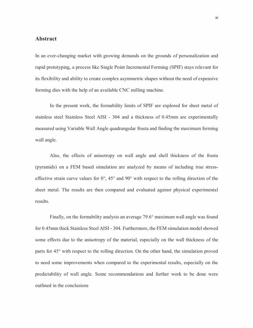
Single Point Incremental Forming (SPIF), is a type of deformation process, inside the
classification of shaping processes, in which sheet metal parts are progressively deformed
often with a semispherical tool into a desired shape, while it is being held in place by a blank
holder.
Incremental sheet forming is defined by Jeswiet (2005) as a process which has a solid,
small-sized tool, instead of large, dedicated dies like in the case of stamping. The forming
tool is in continuous contact with sheet metal and moves in 3-dimensional space under control
in order to produce asymmetric sheet metal shapes. SPIF is the variant that utilizes a single
point for deformation, as opposed to processes that use two points, one on top and one on the
bottom of the sheet to support the process.
Figure 1. SPIF tool, blank holder, and lubricated blank
2
As many researchers have pointed out, the main advantage of SPIF is that there is no need
for expensive customized dies as in conventional stamping. SPIF has the capability of
producing prototype parts of very complex and asymmetrical shape without the need of a
strong initial investment, as long as there is a CNC mill available for use (McAnulty, Jeswiet,
& Doolan, 2016).
Nonetheless, the high amount of time it takes to form one part prevents it from directly
competing against conventional stamping. Instead, its purpose is to complement it with the
possibility of producing small batch sizes and single pieces of highly personalized parts
(Perez Santiago, 2012).
A more comprehensive analysis of the classification and characteristics of this process
has been recently done by Arturo Belmont (Belmont Galvez, 2018) on a thesis belonging to
the same investigation program as the present work. In his thesis, Belmont-Galvez presented
how SPIF came to form part of the performable mechanical processes at UDLAP, and also a
general comparison with conventional stamping. Please refer to the mentioned work for
further information on the topic.
3
1.1 Thesis Topic and Justification
The main topic of this work is the Single Point variant of Incremental Forming, for short
SPIF, done on Stainless Steel AISI - 304 sheet metal of a thickness 0.45mm. The specific
aspects of this process researched are two. First, its modeling and simulation by means of
Finite Element Method (FEM) simulation with considerations of anisotropy. Second, the
Formability by means of defining the maximum wall angle at which a part can be formed.
Research on anisotropy’s effects on FEM simulation of SPIF have not been performed
on Stainless Steel AISI - 304. Although the formability of this material has already been
studied by both Centeno (2014) and Golabi(2014), it has not been done for such a small
thickness.
The reason for a sheet metal thickness of relatively small size (0.45 mm) compared
to the mainstream of research done, is because of the machine limitations of having a CNC
machining mill for educational purposes, in this case an EMCO 500 Concept Mill. There is
a strong relationship between the axial force on the tool, and the thickness of the material as
presented by (Perez Santiago, 2012). On his work, Perez Santiago uses Aerens’ equation for
steady state to predict dynamic axial forces and determined them to have good results.
Aerens’ equation is provided below as equation 1, where Rm is the materials tensile strength,
t is the sheet thickness, d is the tools diameter, Δh is the scallop height11 and α is the forming
angle.
1. 1 Scallop height: height of the localized impression of the forming tool on the plane of the
sheet being formed (Perez Santiago, 2012)
4
Therefore, research done on small thickness materials can provide useful information
for institutions with small CNC milling equipment to conduct research on SPIF.
(1)
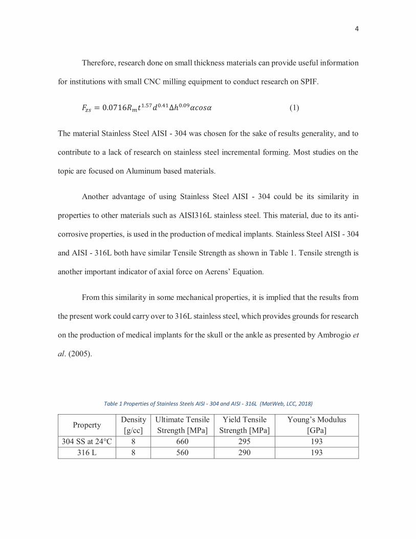
The material Stainless Steel AISI - 304 was chosen for the sake of results generality, and to
contribute to a lack of research on stainless steel incremental forming. Most studies on the
topic are focused on Aluminum based materials.
Another advantage of using Stainless Steel AISI - 304 could be its similarity in
properties to other materials such as AISI316L stainless steel. This material, due to its anti-
corrosive properties, is used in the production of medical implants. Stainless Steel AISI - 304
and AISI - 316L both have similar Tensile Strength as shown in Table 1. Tensile strength is
another important indicator of axial force on Aerens’ Equation.
From this similarity in some mechanical properties, it is implied that the results from
the present work could carry over to 316L stainless steel, which provides grounds for research
on the production of medical implants for the skull or the ankle as presented by Ambrogio et
al. (2005).
Table 1 Properties of Stainless Steels AISI - 304 and AISI - 316L (MatWeb, LCC, 2018)
Property Density [g/cc]
Ultimate Tensile Strength [MPa]
Yield Tensile Strength [MPa]
Young’s Modulus [GPa]
304 SS at 24°C 8 660 295 193 316 L 8 560 290 193
5
1.2 Objectives
It is the objective of the present work to improve the research capabilities on Incremental
Forming in La Universidad de las Americas Puebla by providing useful experimental
information that can be applied to the manufacturing of these type of parts.
This is to be achieved by improving and adapting a Finite Element Method simulation
model created by Dr. Rogelio Perez Santiago and by setting a precedent in material
characterization for the Single Point Incremental Forming (SPIF) process with the tools and
machinery available at UDLAP.
Furthermore, it is an objective of this work to find a formability indicator for Stainless
Steel metal sheets during the SPIF process that can aid in future design decisions of more
complex parts.
Therefore, the following research questions are posed to direct this work:
1. Is there a significant anisotropic behavior on the Stainless Steel AISI - 304 sheets
currently used for SPIF forming of parts? And if so, what is its effect on the geometry
formed and effective plastic strain on the part?
2. Is the current Finite Element Method simulation model being used suitable for
predicting the geometry of manufactured parts?
3. What is the maximum forming angle possible for the 0.45 mm thick Stainless Steel
AISI - 304 material with the current tools and machinery at UDLAP?
6
Chapter Two: Literature Review
2.1 Formability in Single Point Incremental Forming (SPIF) Literature Review
Formability as the name implies, is the ability of a material, in this case sheet metal, to be
molded to a desired shape without presenting cracks. Formability is closely related to the
elongation of the material which is the total amount of strain during a process.
Formability in Single Point Incremental Forming (SPIF), commonly named
Spifability has been a topic of discussion for several years. Measuring formability for SPIF
processes has been performed in many ways. Traditionally a forming limit diagram has been
used for this purpose. Alternative methods are for example, the one used by Hussein and Gao
(2007) where they utilized the thinning limits of sheet metals to obtain a quantitative value
for the formability.
In the present work, maximum wall angle has been chosen to describe formability for
its practicality and effectiveness. This method has been used by many researchers including
Hussain, Gao and Ziran (2008), Jeswiet and Micari (Asymmetric Single Point Incremental
Forming of Sheet Metal., 2005). “In SPIF, the maximum forming angle before the occurrence
of fracture is considered as a formability measure of the sheet metal.” (Shamsari, Mirnia,
Elyasi, & Baseri, 2017)
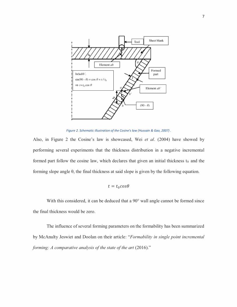
The maximum wall angle is described as the angle between the plane perpendicular
to the axis of the tool used, and the wall being formed. Represented as θ, it can be visualized
in Figure 2.
7
Figure 2. Schematic illustration of the Cosine's law (Hussain & Gao, 2007) .
Also, in Figure 2 the Cosine’s law is showcased, Wei et al. (2004) have showed by
performing several experiments that the thickness distribution in a negative incremental
formed part follow the cosine law, which declares that given an initial thickness t0 and the
forming slope angle θ, the final thickness at said slope is given by the following equation.
With this considered, it can be deduced that a 90° wall angle cannot be formed since
the final thickness would be zero.
The influence of several forming parameters on the formability has been summarized
by McAnulty Jeswiet and Doolan on their article: “Formability in single point incremental
forming: A comparative analysis of the state of the art (2016).”
8
In this article the influence of parameters such as sheet thickness, tool diameter and
shape, feed rate, spindle speed, and step down found by a myriad of researchers was cited
and displayed. Inside this description the material used through each paper was also noted.
Since the material used for the present work is Stainless Steel AISI - 304, special attention
was put on the information for this particular material.
The increase of material thickness was found to have a positive effect on formability
on the research conducted by Golabi. (Golabi & Khazaali, 2014). In this study, a material
thicknesses used were 0.5 and 0.7 mm. In comparison, the sheet metal thickness used for the
present work was 0.45 mm thick. According to Golabi, this would hinder formability.
Tool diameter has a similar effect, its increase in turn yields an increase in formability
as reported by Golabi (2014). On the other hand, Centeno (2014) reported the opposite
relationship between tool diameter and formability. The tool diameters used by Centeno were
6, 10 and 20 mm, while the ones used by Golabi were 6 and 14 mm in diameter. Therefore,
the results are non-conclusive, and instead of being a direct or indirect relationship, tool
diameter must be optimized for a particular set of experiment parameters.
Step down is defined as the movement in the tool’s axial direction after every turn in
incremental forming. As reported by McAnulty et al. (2016) most papers, 13 out of 18,
determined that a decrease in step down meant an improvement in formability. On this
parameter, Golabi (2014) and Centeno (2014) did agree on decreasing the stepdown to
improve formability.
9
The effects of feed rate were found to be non-significant by Golabi (2014). In this
paper 600 and 1200 rpm were used. Papers evaluating the effect of feed rate on Titanium,
AA3003-0, AA2024-T4 and polypropylene, found that a decrease on this parameter
improved formability (McAnulty, Jeswiet, & Doolan, 2016).
Finally, until 2016 the effects of spindle speed on Stainless Steel AISI - 304
formability have not been studied. Nonetheless, most papers for other materials suggest
increasing the spindle speed to increase formability. On the other hand, high spindle speeds
increment tool wear, and demand a higher use of lubricant which has economic and
environmental repercussions.
2.2 Anisotropy in Single Point Incremental Forming (SPIF) Literature Review
Anisotropy is defined as the property of a material to exhibit variations in its physical, or in
this case, mechanical properties along different axes. This is due to the crystallographic
structure and the nature of the rolling process with which sheet metal is manufactured.
Anisotropy is quantified by the Lankford parameter, which is a ratio of the strains in width
and thickness directions during a uniaxial tensile test.
During the review of literature for the preparation of this thesis, an important lack of
information about the effects of anisotropy on the SPIF process was found. In an article
focused of determining the frustum depth of Stainless Steel AISI - 304 stainless steel plates
using incremental forming, the authors briefly mention the effects of anisotropy as non-
10
influential on the process (Golabi & Khazaali, 2014). They do so by citing the work done by
Fratini et al. in 2004 on the influence of mechanical properties on SPIF formability.
Upon further reading of the cited article, the materials used were High Strength Steel,
Deep Drawing Quality steel, AA1050-0, AA6114 T4, Brass and Copper (Fratini, Ambrogio,
Di Lorenzo, Filice, & Micari, 2004). There is no mention of Stainless Steel in this article.
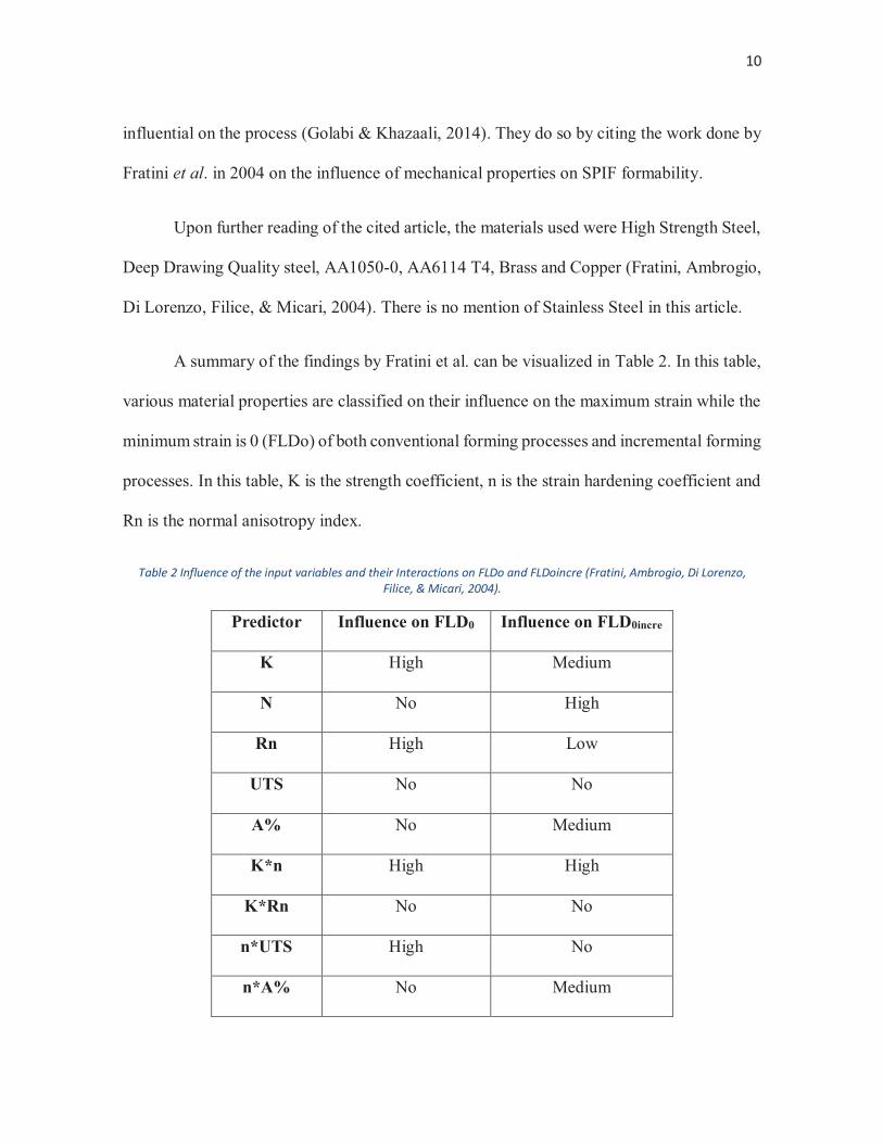
A summary of the findings by Fratini et al. can be visualized in Table 2. In this table,
various material properties are classified on their influence on the maximum strain while the
minimum strain is 0 (FLDo) of both conventional forming processes and incremental forming
processes. In this table, K is the strength coefficient, n is the strain hardening coefficient and
Rn is the normal anisotropy index.
Table 2 Influence of the input variables and their Interactions on FLDo and FLDoincre (Fratini, Ambrogio, Di Lorenzo, Filice, & Micari, 2004).
Predictor Influence on FLD0 Influence on FLD0incre
K High Medium
N No High
Rn High Low
UTS No No
A% No Medium
K*n High High
K*Rn No No
n*UTS High No
n*A% No Medium
11
This Article by Fratini et al. was also disputed by Hussain et al. on the grounds that
few materials were tested and they all had relatively big hardening exponents, therefore their
conclusions could not be generalized. Hussain et al. found that neither K or n are the more
influential parameters on formability, they conclude that the percent tensile reduction of area
is the sole major material property influencing spifability. (Hussain G. , Gao, Hayat, & Ziran,
2008).
Another mention of the effects of anisotropy was found on a more recent study on the
forming behavior of AA-6061 aluminum during SPIF (Kumar Barnwal, Chakrabarty,
Tewari, Narasimhan, & Mishra, 2018). In this article, aluminum sheets were formed into
conical shapes, and the major and minor strains were measured by means of a Digital Image
Correlation method. Also, Finite Element Method simulations were performed to compare
the results. Finally, a detailed microstructural study was carried out, using specimens from
deformed parts of the cone, and intact parts of the cone.
The FEM simulations were done on PAMSTAMP 2G, a commercial software
oriented to the simulation of sheet metal forming. It was performed with a mesh size of 1mm
with four node elements for the blank of sheet metal. The material properties in the FEM
model included a plastic anisotropy factor “r” for the Rolling Direction (RD), 45° to Rolling
Direction (ID), and 90° to rolling direction (TD). These properties are included in Table 3.
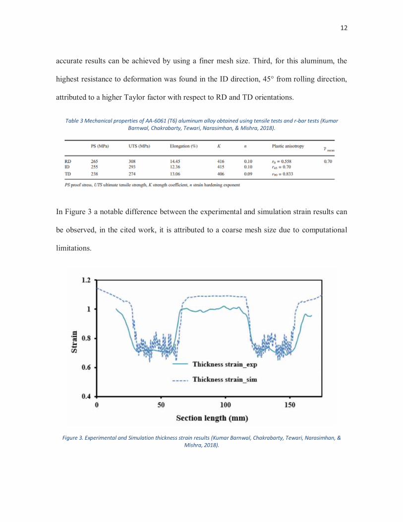
The conclusions reached by Kumar et al. are as follows. First, the major strain during
Single Point incremental forming is always perpendicular to the direction of the tool
movement. Second, FEM results are in accordance to the experimental data but, more
12
accurate results can be achieved by using a finer mesh size. Third, for this aluminum, the
highest resistance to deformation was found in the ID direction, 45° from rolling direction,
attributed to a higher Taylor factor with respect to RD and TD orientations.
Table 3 Mechanical properties of AA-6061 (T6) aluminum alloy obtained using tensile tests and r-bar tests (Kumar Barnwal, Chakrabarty, Tewari, Narasimhan, & Mishra, 2018).
In Figure 3 a notable difference between the experimental and simulation strain results can
be observed, in the cited work, it is attributed to a coarse mesh size due to computational
limitations.
Figure 3. Experimental and Simulation thickness strain results (Kumar Barnwal, Chakrabarty, Tewari, Narasimhan, & Mishra, 2018).

13
From the review of the state of the art on anisotropy it can be concluded that further research
should be conducted. The available information on anisotropy’s effects on formability are
generally performed on aluminum samples. Specific analysis of the effects of anisotropy of
Stainless Steel AISI - 304 was not found.
14
Chapter Three: Methodology
3.1 Characterization Methodology
The material used in the present work is Stainless Steel AISI - 304. Its general properties
were obtained from the available datasheet online (MatWeb, LCC, 2018) which coincides
with the material properties used by other researchers such as Golabi and Khazaali (2014).
These properties are 8 g/cm3 for density, 193 GPa for Young’s modulus and 0.29 for
Poisson’s ratio.
To define the material’s behavior under plastic strain, True Stress vs Effective Plastic
Strain curves were obtained from tensile tests for 0, 45, and 90 degrees with respect to the
rolling direction of the Stainless Steel AISI - 304 sheet metal.
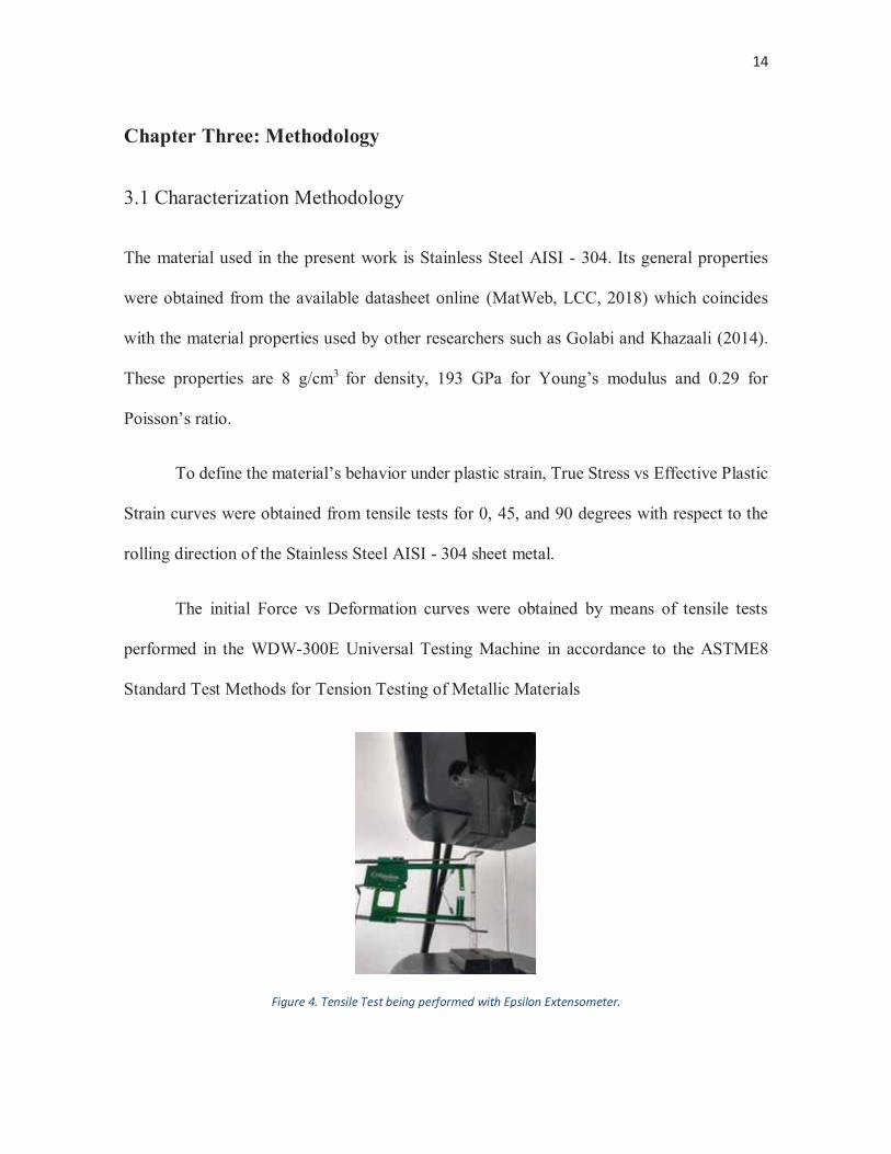
The initial Force vs Deformation curves were obtained by means of tensile tests
performed in the WDW-300E Universal Testing Machine in accordance to the ASTME8
Standard Test Methods for Tension Testing of Metallic Materials
Figure 4. Tensile Test being performed with Epsilon Extensometer.
15
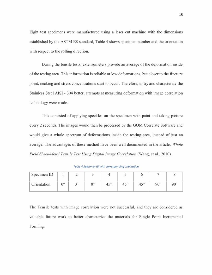
Eight test specimens were manufactured using a laser cut machine with the dimensions
established by the ASTM E8 standard, Table 4 shows specimen number and the orientation
with respect to the rolling direction.
During the tensile tests, extensometers provide an average of the deformation inside
of the testing area. This information is reliable at low deformations, but closer to the fracture
point, necking and stress concentrations start to occur. Therefore, to try and characterize the
Stainless Steel AISI - 304 better, attempts at measuring deformation with image correlation
technology were made.
This consisted of applying speckles on the specimen with paint and taking picture
every 2 seconds. The images would then be processed by the GOM Correlate Software and
would give a whole spectrum of deformations inside the testing area, instead of just an
average. The advantages of these method have been well documented in the article, Whole
Field Sheet-Metal Tensile Test Using Digital Image Correlation (Wang, et al., 2010).
Table 4 Specimen ID with corresponding orientation
Specimen ID 1
2 3 4 5 6 7 8
Orientation 0° 0° 0° 45° 45° 45° 90° 90°
The Tensile tests with image correlation were not successful, and they are considered as
valuable future work to better characterize the materials for Single Point Incremental
Forming.
16
Nonetheless, four successful tensile tests were carried out, with test specimens 2, 4, 5
and 8, with 0°, 45°, 45°, and 90° in orientation respectively.
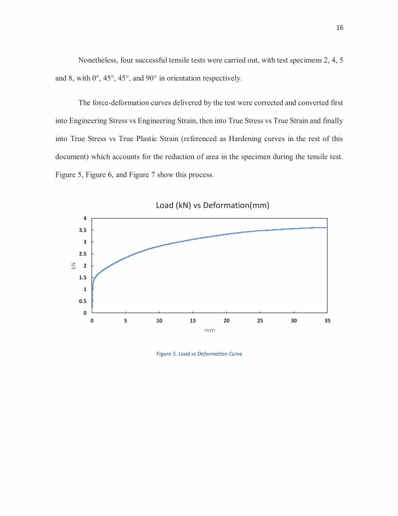
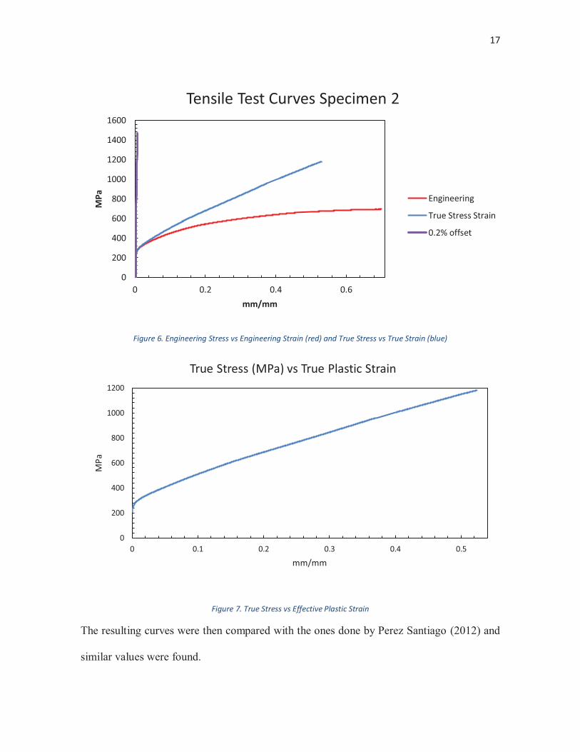
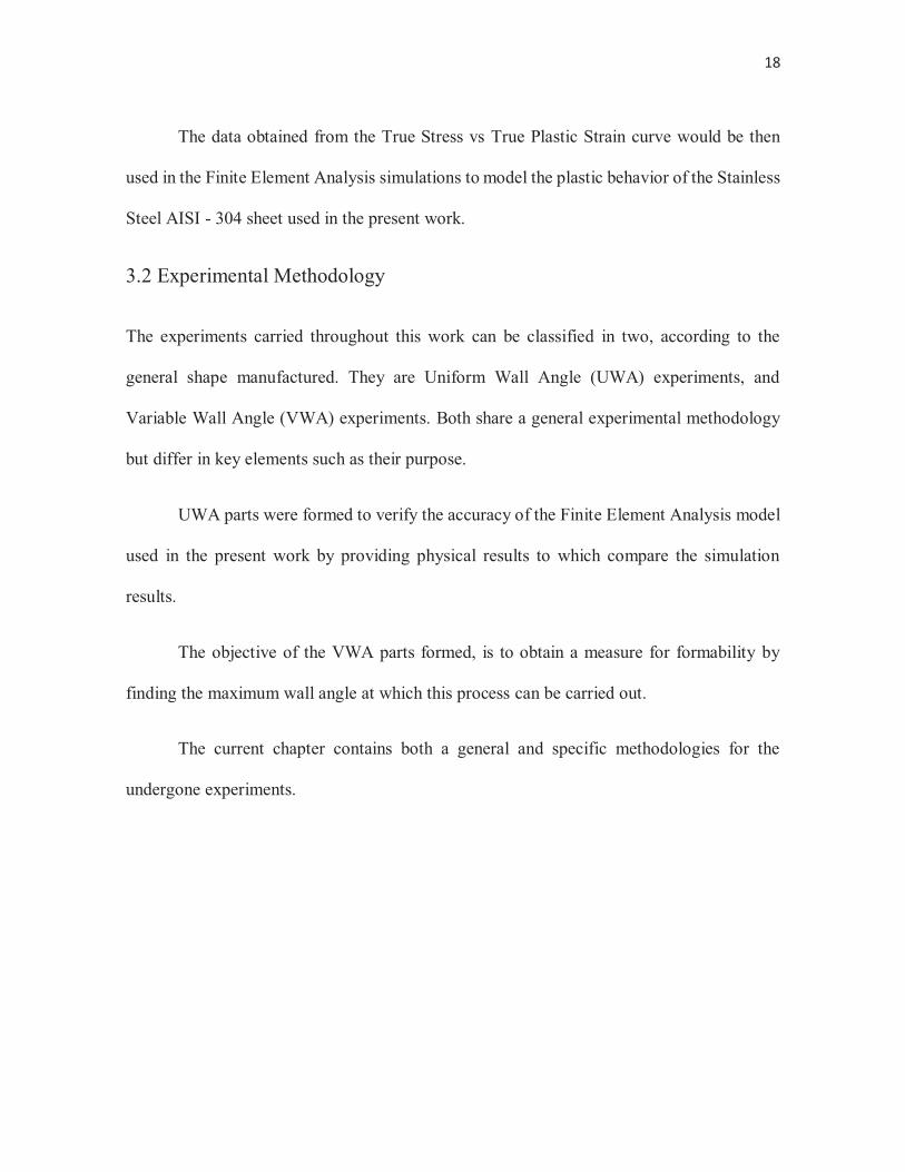
The force-deformation curves delivered by the test were corrected and converted first
into Engineering Stress vs Engineering Strain, then into True Stress vs True Strain and finally
into True Stress vs True Plastic Strain (referenced as Hardening curves in the rest of this
document) which accounts for the reduction of area in the specimen during the tensile test.
Figure 5, Figure 6, and Figure 7 show this process.
Figure 5. Load vs Deformation Curve
0
0.5
1
1.5
2
2.5
3
3.5
4
0 5 10 15 20 25 30 35
kN
mm
Load (kN) vs Deformation(mm)
17
Figure 6. Engineering Stress vs Engineering Strain (red) and True Stress vs True Strain (blue)
Figure 7. True Stress vs Effective Plastic Strain
The resulting curves were then compared with the ones done by Perez Santiago (2012) and
similar values were found.
0
200
400
600
800
1000
1200
1400
1600
0 0.2 0.4 0.6
MPa
mm/mm
Tensile Test Curves Specimen 2
Engineering
True Stress Strain
0.2% offset
0
200
400
600
800
1000
1200
0 0.1 0.2 0.3 0.4 0.5
MPa
mm/mm
True Stress (MPa) vs True Plastic Strain
18
The data obtained from the True Stress vs True Plastic Strain curve would be then
used in the Finite Element Analysis simulations to model the plastic behavior of the Stainless
Steel AISI - 304 sheet used in the present work.
3.2 Experimental Methodology
The experiments carried throughout this work can be classified in two, according to the
general shape manufactured. They are Uniform Wall Angle (UWA) experiments, and
Variable Wall Angle (VWA) experiments. Both share a general experimental methodology
but differ in key elements such as their purpose.
UWA parts were formed to verify the accuracy of the Finite Element Analysis model
used in the present work by providing physical results to which compare the simulation
results.
The objective of the VWA parts formed, is to obtain a measure for formability by
finding the maximum wall angle at which this process can be carried out.
The current chapter contains both a general and specific methodologies for the
undergone experiments.
19
3.2.1 General SPIF Methodology
Several parts were formed during the course of the present work, and a general experimental
methodology was used for all of them.
First, the desired geometrical, or product, parameters were defined, this include the
initial sheet thickness, the general shape (cone, pyramid), type of wall (variable wall angle
or uniform wall angle), width of the pyramid at the top (diameter in the case of a cone), the
initial forming angle, the stepdown (tool pitch), the amount of steps which define the height
of the part, and generatrix radius (zero for uniform wall angle parts).
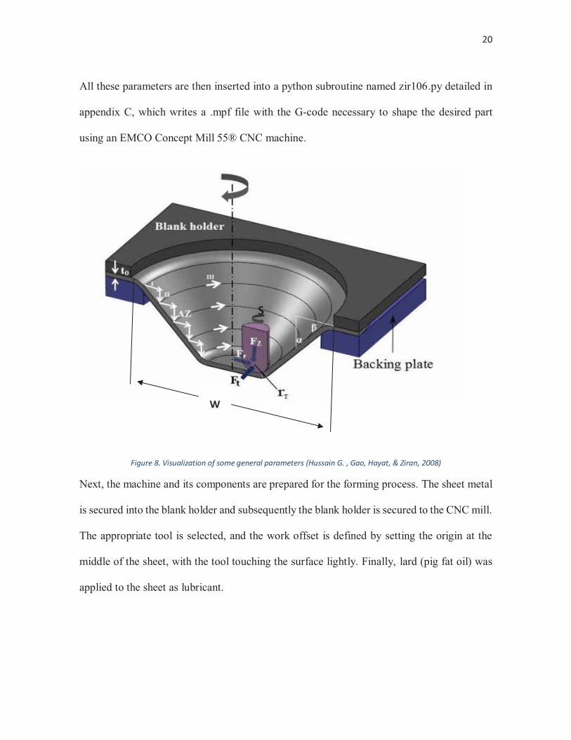
Then, the process parameters are defined. These are tool radius, spindle speed, feed rate and
lubrication rate. These parameters along with the geometrical parameters can be seen in Table
5. In Figure 8 some of these parameters are also depicted.
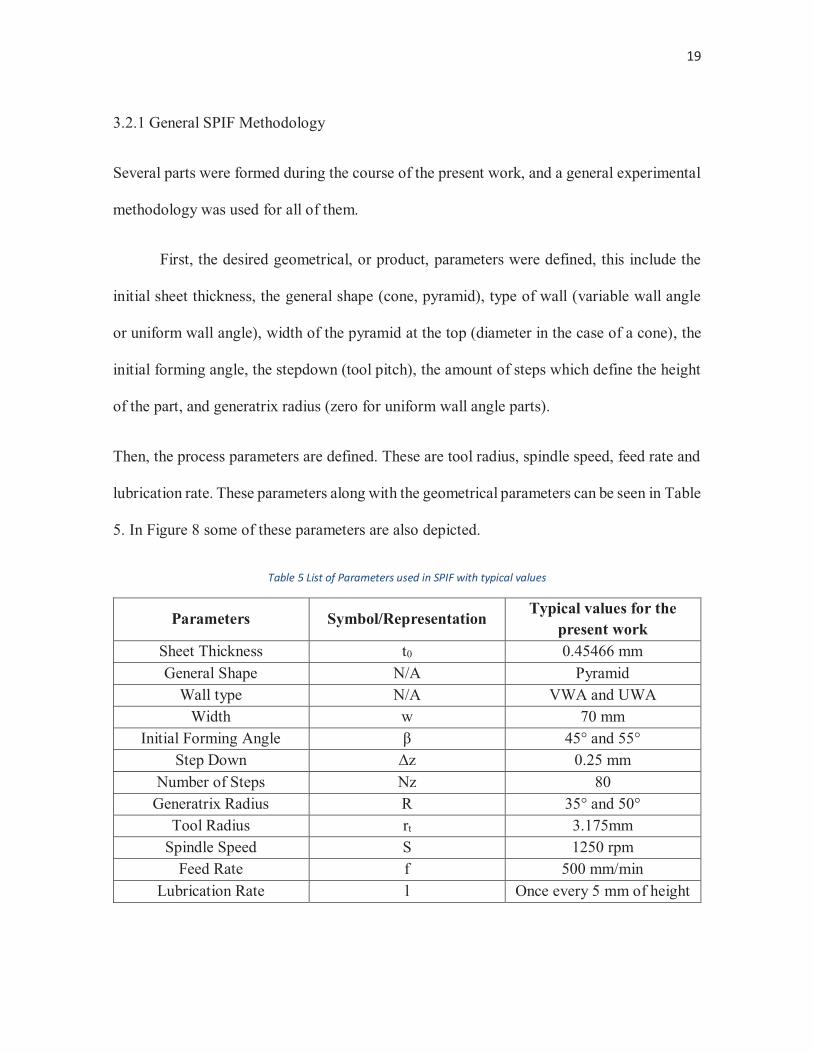
Table 5 List of Parameters used in SPIF with typical values
Parameters Symbol/Representation Typical values for the present work
Sheet Thickness t0 0.45466 mm General Shape N/A Pyramid
Wall type N/A VWA and UWA Width w 70 mm
Initial Forming Angle β 45° and 55° Step Down Δz 0.25 mm
Number of Steps Nz 80 Generatrix Radius R 35° and 50°
Tool Radius rt 3.175mm Spindle Speed S 1250 rpm
Feed Rate f 500 mm/min Lubrication Rate l Once every 5 mm of height
20
All these parameters are then inserted into a python subroutine named zir106.py detailed in
appendix C, which writes a .mpf file with the G-code necessary to shape the desired part
using an EMCO Concept Mill 55® CNC machine.
Figure 8. Visualization of some general parameters (Hussain G. , Gao, Hayat, & Ziran, 2008)
Next, the machine and its components are prepared for the forming process. The sheet metal
is secured into the blank holder and subsequently the blank holder is secured to the CNC mill.
The appropriate tool is selected, and the work offset is defined by setting the origin at the
middle of the sheet, with the tool touching the surface lightly. Finally, lard (pig fat oil) was
applied to the sheet as lubricant.
S
w
21
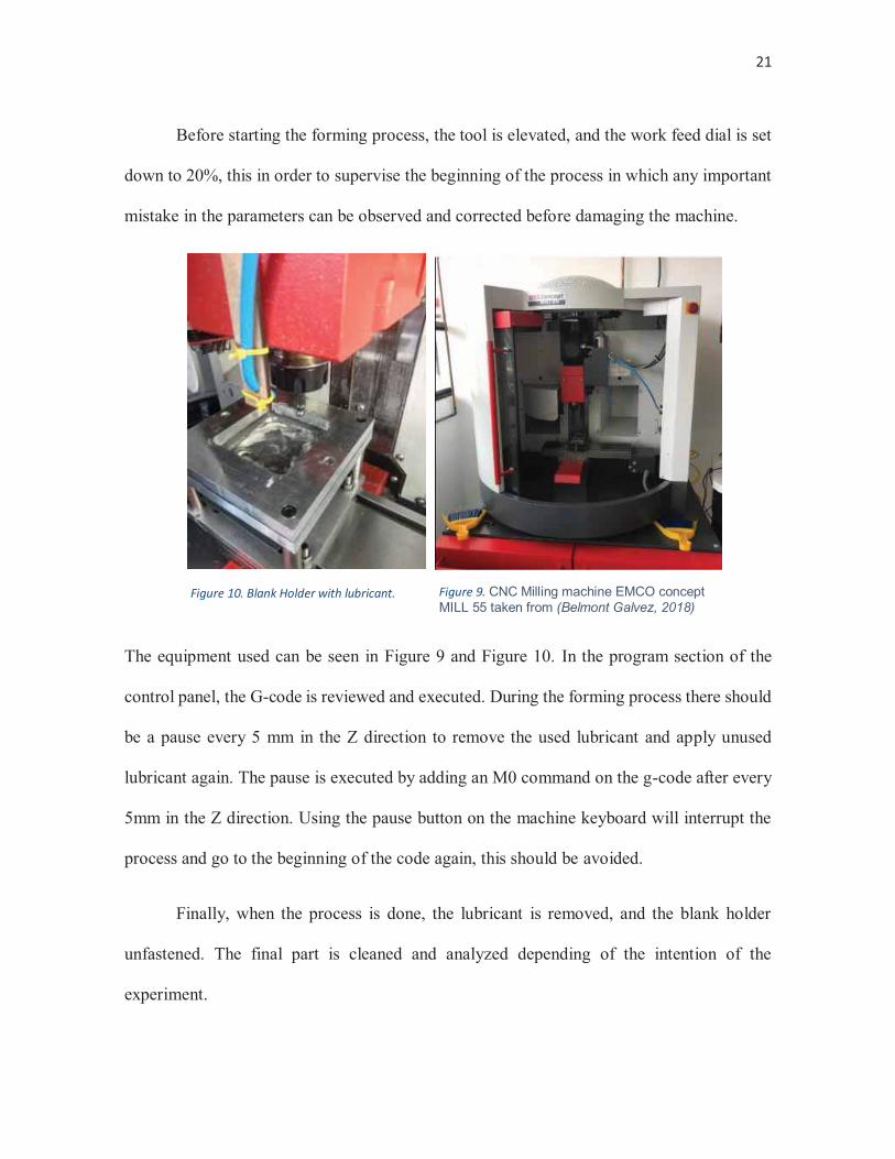
Before starting the forming process, the tool is elevated, and the work feed dial is set
down to 20%, this in order to supervise the beginning of the process in which any important
mistake in the parameters can be observed and corrected before damaging the machine.
The equipment used can be seen in Figure 9 and Figure 10. In the program section of the
control panel, the G-code is reviewed and executed. During the forming process there should
be a pause every 5 mm in the Z direction to remove the used lubricant and apply unused
lubricant again. The pause is executed by adding an M0 command on the g-code after every
5mm in the Z direction. Using the pause button on the machine keyboard will interrupt the
process and go to the beginning of the code again, this should be avoided.
Finally, when the process is done, the lubricant is removed, and the blank holder
unfastened. The final part is cleaned and analyzed depending of the intention of the
experiment.
Figure 10. Blank Holder with lubricant. Figure 9. CNC Milling machine EMCO concept MILL 55 taken from (Belmont Galvez, 2018)
22
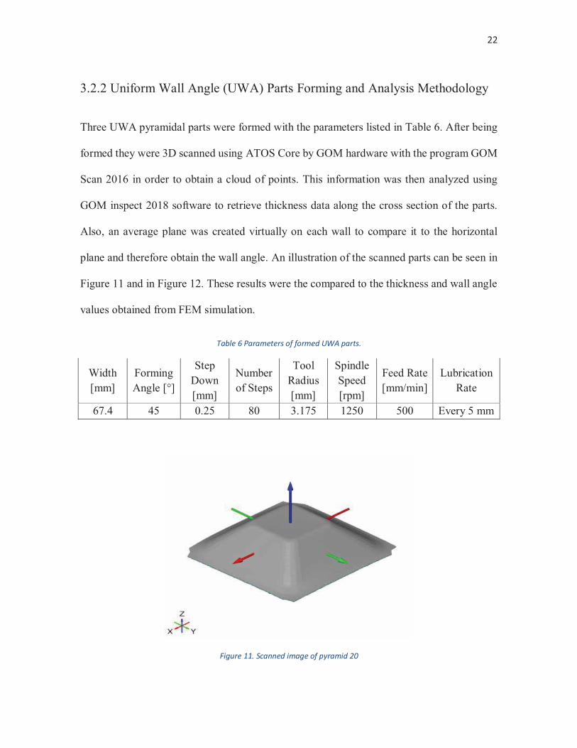
3.2.2 Uniform Wall Angle (UWA) Parts Forming and Analysis Methodology
Three UWA pyramidal parts were formed with the parameters listed in Table 6. After being
formed they were 3D scanned using ATOS Core by GOM hardware with the program GOM
Scan 2016 in order to obtain a cloud of points. This information was then analyzed using
GOM inspect 2018 software to retrieve thickness data along the cross section of the parts.
Also, an average plane was created virtually on each wall to compare it to the horizontal
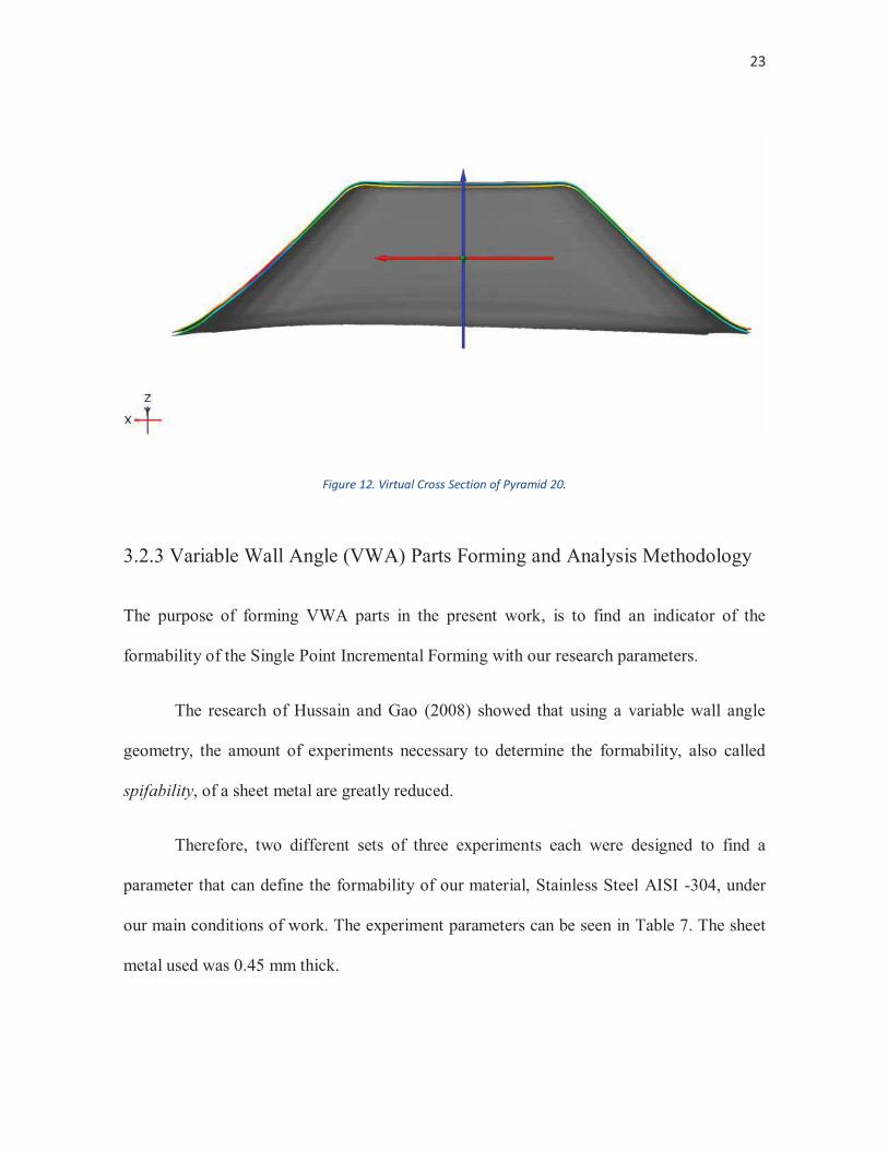
plane and therefore obtain the wall angle. An illustration of the scanned parts can be seen in
Figure 11 and in Figure 12. These results were the compared to the thickness and wall angle
values obtained from FEM simulation.
Table 6 Parameters of formed UWA parts.
Width [mm]
Forming Angle [°]
Step Down [mm]
Number of Steps
Tool Radius [mm]
Spindle Speed [rpm]
Feed Rate [mm/min]
Lubrication Rate
67.4 45 0.25 80 3.175 1250 500 Every 5 mm
Figure 11. Scanned image of pyramid 20
23
Figure 12. Virtual Cross Section of Pyramid 20.
3.2.3 Variable Wall Angle (VWA) Parts Forming and Analysis Methodology
The purpose of forming VWA parts in the present work, is to find an indicator of the
formability of the Single Point Incremental Forming with our research parameters.
The research of Hussain and Gao (2008) showed that using a variable wall angle
geometry, the amount of experiments necessary to determine the formability, also called
spifability, of a sheet metal are greatly reduced.
Therefore, two different sets of three experiments each were designed to find a
parameter that can define the formability of our material, Stainless Steel AISI -304, under
our main conditions of work. The experiment parameters can be seen in Table 7. The sheet
metal used was 0.45 mm thick.
24
Table 7 Experiment Parameters for Sets A and B.
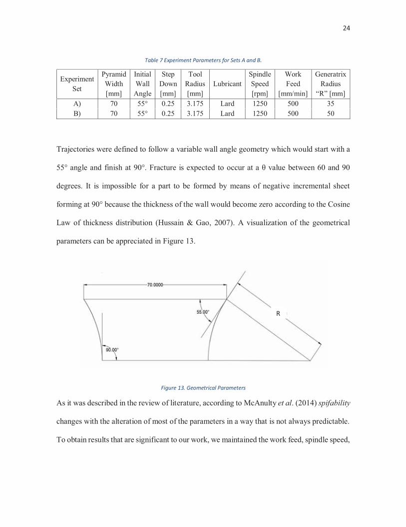
Trajectories were defined to follow a variable wall angle geometry which would start with a
55° angle and finish at 90°. Fracture is expected to occur at a θ value between 60 and 90
degrees. It is impossible for a part to be formed by means of negative incremental sheet
forming at 90° because the thickness of the wall would become zero according to the Cosine
Law of thickness distribution (Hussain & Gao, 2007). A visualization of the geometrical
parameters can be appreciated in Figure 13.
Figure 13. Geometrical Parameters
As it was described in the review of literature, according to McAnulty et al. (2014) spifability
changes with the alteration of most of the parameters in a way that is not always predictable.
To obtain results that are significant to our work, we maintained the work feed, spindle speed,
Experiment Set
Pyramid Width [mm]
Initial Wall
Angle
Step Down [mm]
Tool Radius [mm]
Lubricant Spindle Speed [rpm]
Work Feed
[mm/min]
Generatrix Radius
“R” [mm] A) 70 55° 0.25 3.175 Lard 1250 500 35 B) 70 55° 0.25 3.175 Lard 1250 500 50
R
25
lubricant, tool radius and step down in accordance to the rest of the experiments performed
throughout this work.
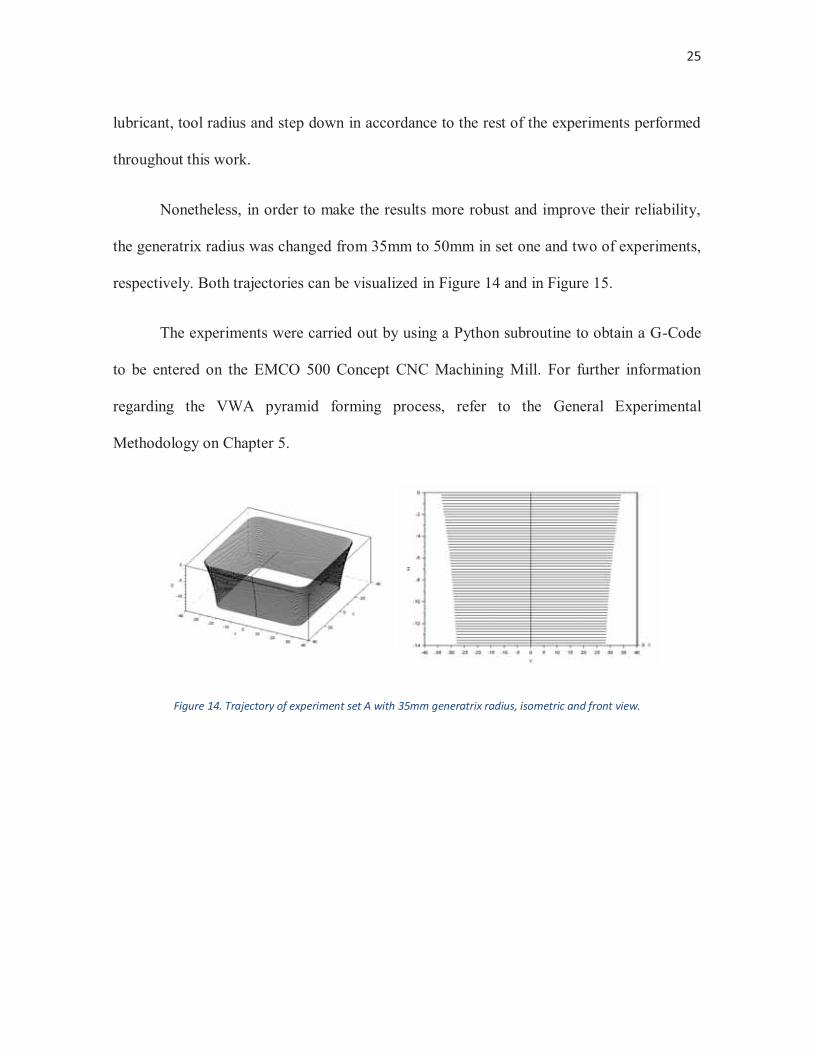
Nonetheless, in order to make the results more robust and improve their reliability,
the generatrix radius was changed from 35mm to 50mm in set one and two of experiments,
respectively. Both trajectories can be visualized in Figure 14 and in Figure 15.
The experiments were carried out by using a Python subroutine to obtain a G-Code
to be entered on the EMCO 500 Concept CNC Machining Mill. For further information
regarding the VWA pyramid forming process, refer to the General Experimental
Methodology on Chapter 5.
Figure 14. Trajectory of experiment set A with 35mm generatrix radius, isometric and front view.
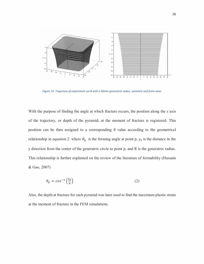
26
Figure 15. Trajectory of experiment set B with a 50mm generatrix radius, isometric and front view.
With the purpose of finding the angle at which fracture occurs, the position along the z axis
of the trajectory, or depth of the pyramid, at the moment of fracture is registered. This
position can be then assigned to a corresponding θ value according to the geometrical
relationship in equation 2. where is the forming angle at point p, yp is the distance in the
y direction from the center of the generatrix circle to point p, and R is the generatrix radius.
This relationship is further explained on the review of the literature of formability (Hussain
& Gao, 2007)
(2)
Also, the depth at fracture for each pyramid was later used to find the maximum plastic strain
at the moment of fracture in the FEM simulations.
27
3.3 Finite Element Analysis Methodology
The FEM model was created by Perez-Santiago for his Ph.D. dissertation in 2012. This model
and methodology has been modified and improved to fit the context research at Universidad
de las Americas Puebla.
3.3.1 Finite Element Analysis Methodology in General
In this thesis, the finite element analysis (FEA) was used to simulate the Single Point
Incremental Forming Process with the specifications particular to the equipment available in
La Universidad de Las Americas Puebla, although it can be adapted to processes done
elsewhere.
This general FEA Methodology applies for the subsequent chapters on Simulation
Methodology.
28
3.3.1.1 Parts definition
The steps taken to perform simulations using FEA started with the computer assisted drawing
of our setup using the software CREO Parametric 4.0®. These drawings included the tool
with its clamping device, the blank holder and the blank. Each of these components would
become the three parts involved in the FEA.
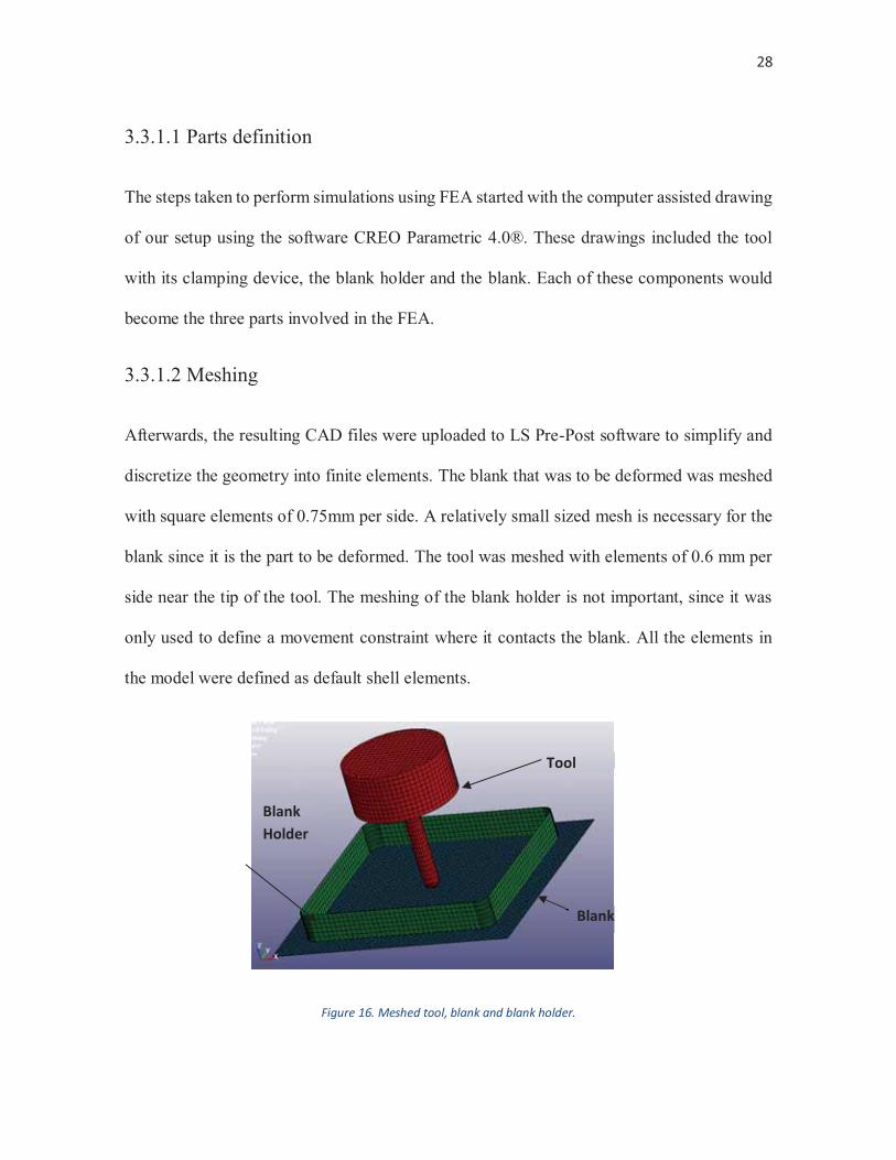
3.3.1.2 Meshing
Afterwards, the resulting CAD files were uploaded to LS Pre-Post software to simplify and
discretize the geometry into finite elements. The blank that was to be deformed was meshed
with square elements of 0.75mm per side. A relatively small sized mesh is necessary for the
blank since it is the part to be deformed. The tool was meshed with elements of 0.6 mm per
side near the tip of the tool. The meshing of the blank holder is not important, since it was
only used to define a movement constraint where it contacts the blank. All the elements in
the model were defined as default shell elements.
Figure 16. Meshed tool, blank and blank holder.
Blank Holder
Tool
Blank
29
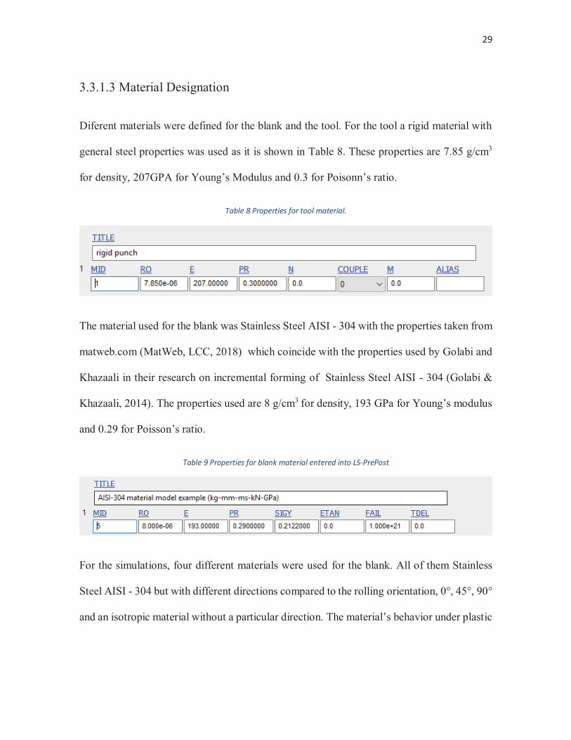
3.3.1.3 Material Designation
Diferent materials were defined for the blank and the tool. For the tool a rigid material with
general steel properties was used as it is shown in Table 8. These properties are 7.85 g/cm3
for density, 207GPA for Young’s Modulus and 0.3 for Poisonn’s ratio.
Table 8 Properties for tool material.
The material used for the blank was Stainless Steel AISI - 304 with the properties taken from
matweb.com (MatWeb, LCC, 2018) which coincide with the properties used by Golabi and
Khazaali in their research on incremental forming of Stainless Steel AISI - 304 (Golabi &
Khazaali, 2014). The properties used are 8 g/cm3 for density, 193 GPa for Young’s modulus
and 0.29 for Poisson’s ratio.
Table 9 Properties for blank material entered into LS-PrePost
For the simulations, four different materials were used for the blank. All of them Stainless
Steel AISI - 304 but with different directions compared to the rolling orientation, 0°, 45°, 90°
and an isotropic material without a particular direction. The material’s behavior under plastic
30
deformation was inserted into the simulation by adding the values of the strain hardening
curve obtained with tensile tests for all three directions.
3.3.1.4 Boundary Conditions
The blank was constrained in the nodes that were in contact or outside the blank holder to
simulate the function of the real blank holder. The constraint was fixed in all three directions
and rotations.
The contact between the blank and the tool was defined as “contact forming one way
surface to surface” which defines a master surface (tool) and a slave surface (blank).
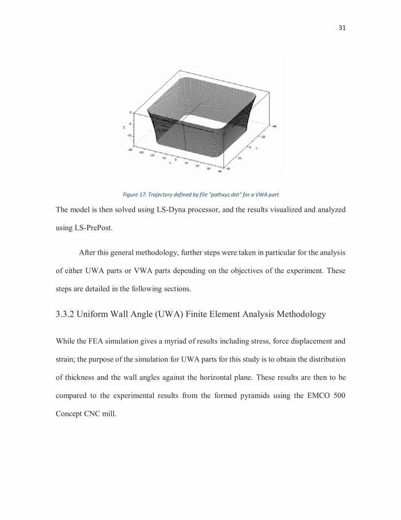
3.3.1.5 Prescribed Motion.
The motion of the tool is given by velocity curves that define the movement in x, y and z
directions of the tool. These curves are obtained by runing the second python subroutine
called velzir5b.py ,which is included in appendix C, after obtaining the coordinate file
“pathxyz.dat” by running the first python subroutine “zir106.py” ,also included in appendix
C, with the desired parameters as described in Chapter 3.2.1.
31
Figure 17. Trajectory defined by file "pathxyz.dat" for a VWA part
The model is then solved using LS-Dyna processor, and the results visualized and analyzed
using LS-PrePost.
After this general methodology, further steps were taken in particular for the analysis
of either UWA parts or VWA parts depending on the objectives of the experiment. These
steps are detailed in the following sections.
3.3.2 Uniform Wall Angle (UWA) Finite Element Analysis Methodology
While the FEA simulation gives a myriad of results including stress, force displacement and
strain; the purpose of the simulation for UWA parts for this study is to obtain the distribution
of thickness and the wall angles against the horizontal plane. These results are then to be
compared to the experimental results from the formed pyramids using the EMCO 500
Concept CNC mill.
32
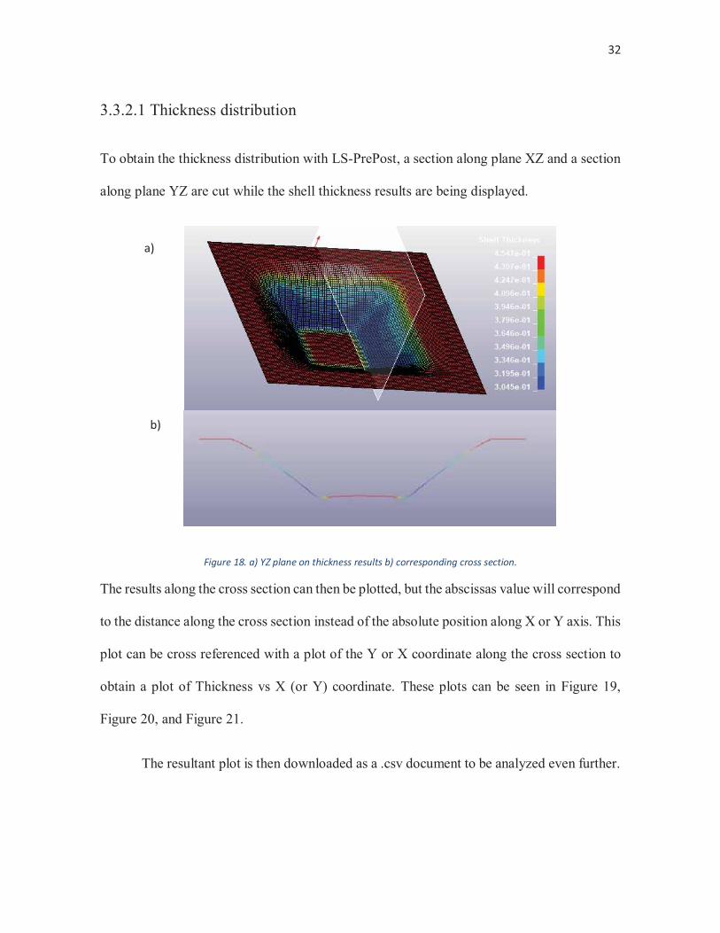
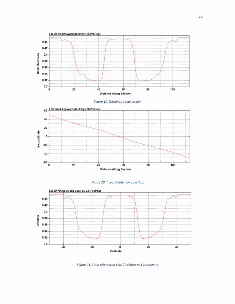
3.3.2.1 Thickness distribution
To obtain the thickness distribution with LS-PrePost, a section along plane XZ and a section
along plane YZ are cut while the shell thickness results are being displayed.
Figure 18. a) YZ plane on thickness results b) corresponding cross section.
The results along the cross section can then be plotted, but the abscissas value will correspond
to the distance along the cross section instead of the absolute position along X or Y axis. This
plot can be cross referenced with a plot of the Y or X coordinate along the cross section to
obtain a plot of Thickness vs X (or Y) coordinate. These plots can be seen in Figure 19,
Figure 20, and Figure 21.
The resultant plot is then downloaded as a .csv document to be analyzed even further.
a)
b)
33
Figure 19. Thickness along section
Figure 20. Y coordinate along section.
Figure 21. Cross referenced plot. Thickness vs Y coordinate
34
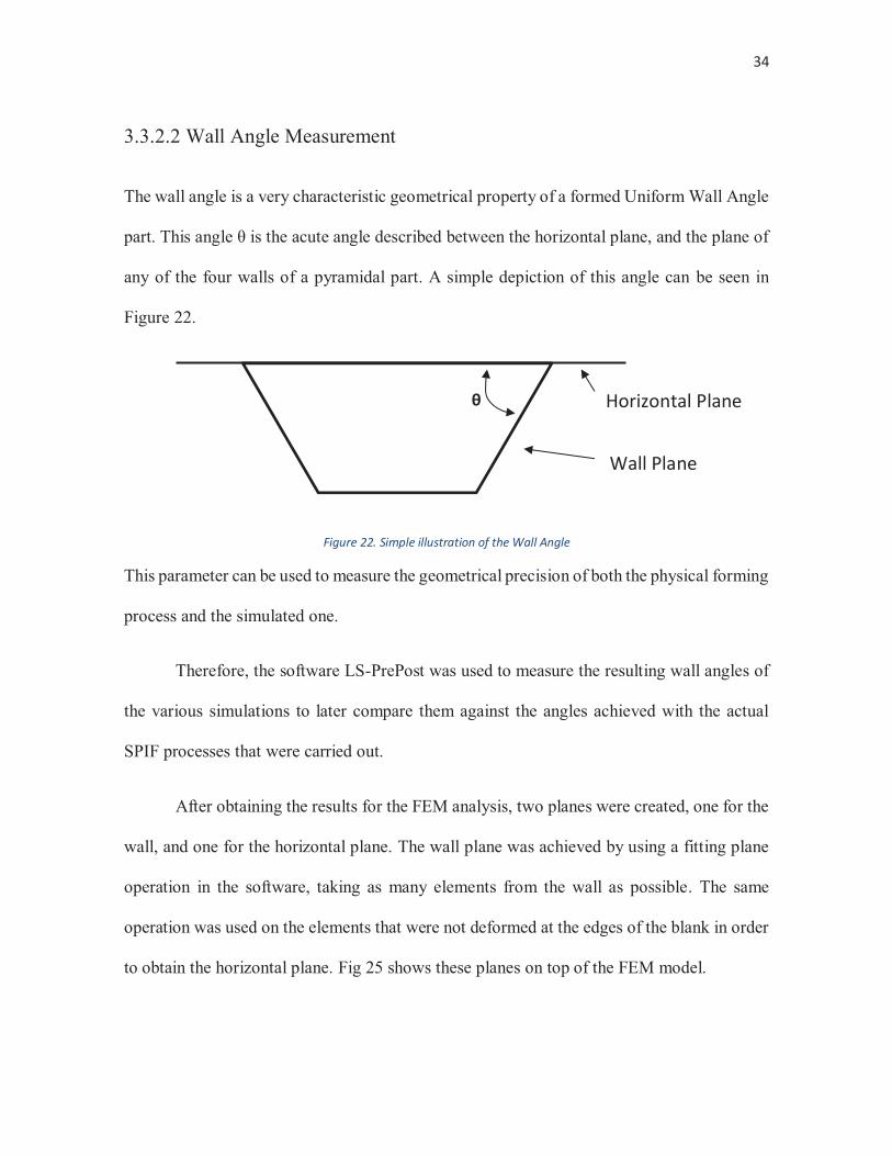
3.3.2.2 Wall Angle Measurement
The wall angle is a very characteristic geometrical property of a formed Uniform Wall Angle
part. This angle θ is the acute angle described between the horizontal plane, and the plane of
any of the four walls of a pyramidal part. A simple depiction of this angle can be seen in
Figure 22.
Figure 22. Simple illustration of the Wall Angle
This parameter can be used to measure the geometrical precision of both the physical forming
process and the simulated one.
Therefore, the software LS-PrePost was used to measure the resulting wall angles of
the various simulations to later compare them against the angles achieved with the actual
SPIF processes that were carried out.
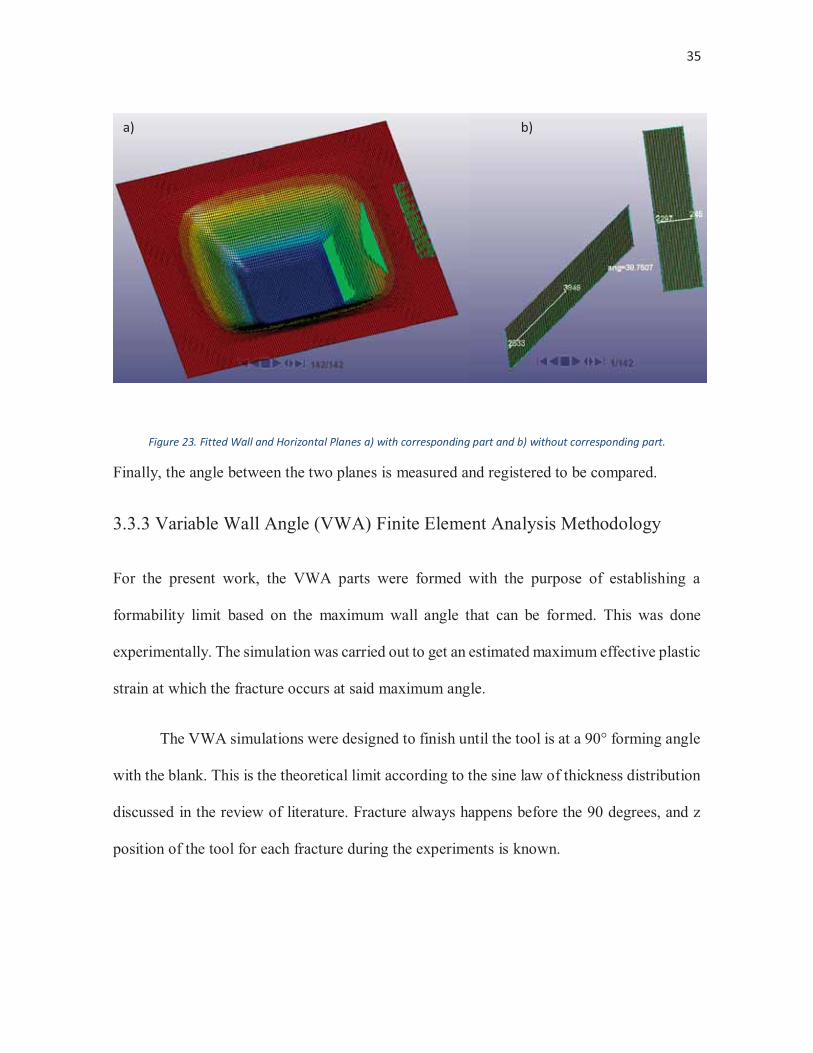
After obtaining the results for the FEM analysis, two planes were created, one for the
wall, and one for the horizontal plane. The wall plane was achieved by using a fitting plane
operation in the software, taking as many elements from the wall as possible. The same
operation was used on the elements that were not deformed at the edges of the blank in order
to obtain the horizontal plane. Fig 25 shows these planes on top of the FEM model.
Horizontal Plane θ
Wall Plane
35
Figure 23. Fitted Wall and Horizontal Planes a) with corresponding part and b) without corresponding part.
Finally, the angle between the two planes is measured and registered to be compared.
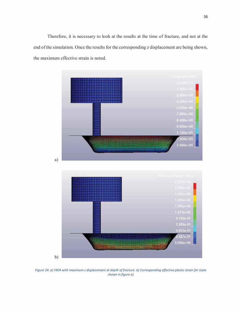
3.3.3 Variable Wall Angle (VWA) Finite Element Analysis Methodology
For the present work, the VWA parts were formed with the purpose of establishing a
formability limit based on the maximum wall angle that can be formed. This was done
experimentally. The simulation was carried out to get an estimated maximum effective plastic
strain at which the fracture occurs at said maximum angle.
The VWA simulations were designed to finish until the tool is at a 90° forming angle
with the blank. This is the theoretical limit according to the sine law of thickness distribution
discussed in the review of literature. Fracture always happens before the 90 degrees, and z
position of the tool for each fracture during the experiments is known.
a) b)
36
Therefore, it is necessary to look at the results at the time of fracture, and not at the
end of the simulation. Once the results for the corresponding z displacement are being shown,
the maximum effective strain is noted.
a)
b)
Figure 24. a) VWA with maximum z displacement at depth of fracture. b) Corresponding effective plastic strain for state shown in figure a)
37
Chapter Four: Results and Discussion
In this Chapter, the results for the Characterization Process, the Uniform Wall Angle
and Variable Wall Angle experiments will be presented and discussed. The experimental
results of both type of parts will be compared to their respective simulation.
4.1 Characterization Results
Four Tensile Tests were carried out for specimens 2, 4, 5, and 8 with 0°, 45°, 45°, and 90°
orientation with respect to the rolling direction of the sheet metal. The resulting Load vs
Deformation and analogous True Stress – True Plastic Strain are presented on appendix A in
figures 65 through 72.
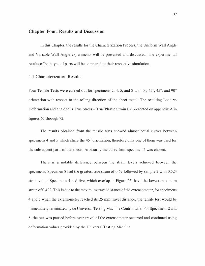
The results obtained from the tensile tests showed almost equal curves between
specimens 4 and 5 which share the 45° orientation, therefore only one of them was used for
the subsequent parts of this thesis. Arbitrarily the curve from specimen 5 was chosen.
There is a notable difference between the strain levels achieved between the
specimens. Specimen 8 had the greatest true strain of 0.62 followed by sample 2 with 0.524
strain value. Specimens 4 and five, which overlap in Figure 25, have the lowest maximum
strain of 0.422. This is due to the maximum travel distance of the extensometer, for specimens
4 and 5 when the extensometer reached its 25 mm travel distance, the tensile test would be
immediately terminated by de Universal Testing Machine Control Unit. For Specimens 2 and
8, the test was paused before over-travel of the extensometer occurred and continued using
deformation values provided by the Universal Testing Machine.
38
Therefore, this differences in maximum strain before fracture are only significant
between specimens 2 and 8.
The yield stress for each specimen is noted in Table 10. This value is where the trues
stress vs strain hardening curve starts, therefore, during the simulation the behavior of the
material will be modeled according to the Young’s Modulus until the stress experimented by
an element reaches the yield stress. After that point the material’s behavior will be modeled
after the True Stress vs Effective Plastic Strain curve.
Table 10 Yield Stress for each Specimen
Specimen 2 4 5 8 Yield Stress(MPa) 211.63 209.1 208.29 217.53
Figure 25. Comparison of True Stress vs True Strain Curves
0
200
400
600
800
1000
1200
1400
0 0.1 0.2 0.3 0.4 0.5 0.6
MPa
mm/mm
True Stress (MPa) vs True Strain (mm/mm)
Sample2_0°
Sample8_90°
Sample5_45°
Sample4_45°
39
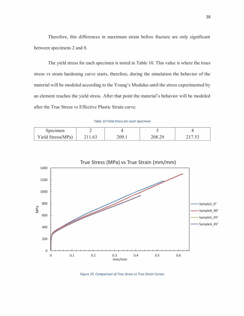
Figure 26. True Stress vs Effective Plastic Strain curves inserted in LS-PrePost; purple 0°, red 90° and yellow 45°
4.2 Uniform Wall Angle (UWA) Results
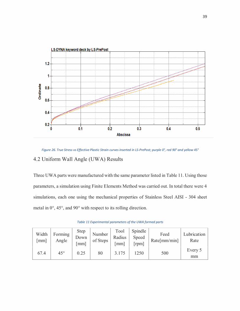
Three UWA parts were manufactured with the same parameter listed in Table 11. Using those
parameters, a simulation using Finite Elements Method was carried out. In total there were 4
simulations, each one using the mechanical properties of Stainless Steel AISI - 304 sheet
metal in 0°, 45°, and 90° with respect to its rolling direction.
Table 11 Experimental parameters of the UWA formed parts
Width [mm]
Forming Angle
Step Down [mm]
Number of Steps
Tool Radius [mm]
Spindle Speed [rpm]
Feed Rate[mm/min]
Lubrication Rate
67.4 45° 0.25 80 3.175 1250 500 Every 5
mm
40
These experiments were performed to determine the influence of anisotropy of the Stainless
Steel AISI - 304 sheet metal of 0.45 mm of thickness during the simulations. The following
sections depict the experimental and simulation results and a comparison between both to
determine the accuracy of the simulation model.
4.2.1 UWA Experimental Results
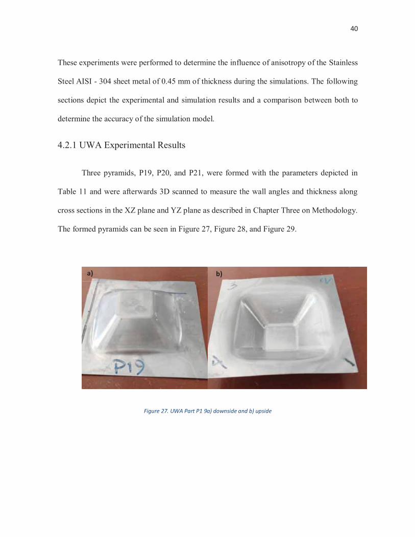
Three pyramids, P19, P20, and P21, were formed with the parameters depicted in
Table 11 and were afterwards 3D scanned to measure the wall angles and thickness along
cross sections in the XZ plane and YZ plane as described in Chapter Three on Methodology.
The formed pyramids can be seen in Figure 27, Figure 28, and Figure 29.
Figure 27. UWA Part P1 9a) downside and b) upside
a) b)
41
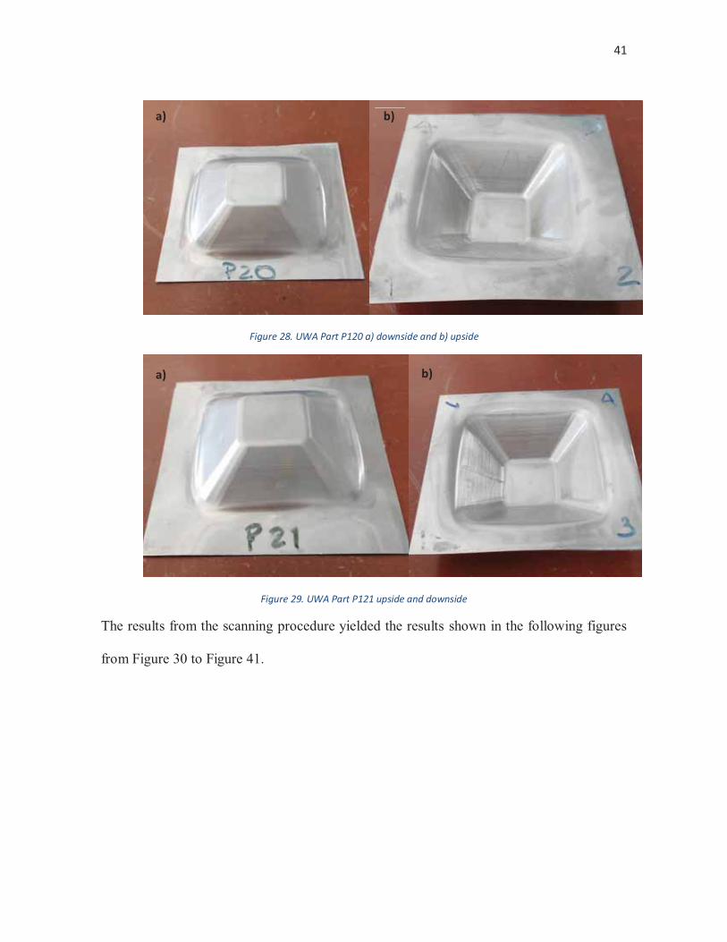
Figure 28. UWA Part P120 a) downside and b) upside
Figure 29. UWA Part P121 upside and downside
The results from the scanning procedure yielded the results shown in the following figures
from Figure 30 to Figure 41.
a) b)
a) b)
42
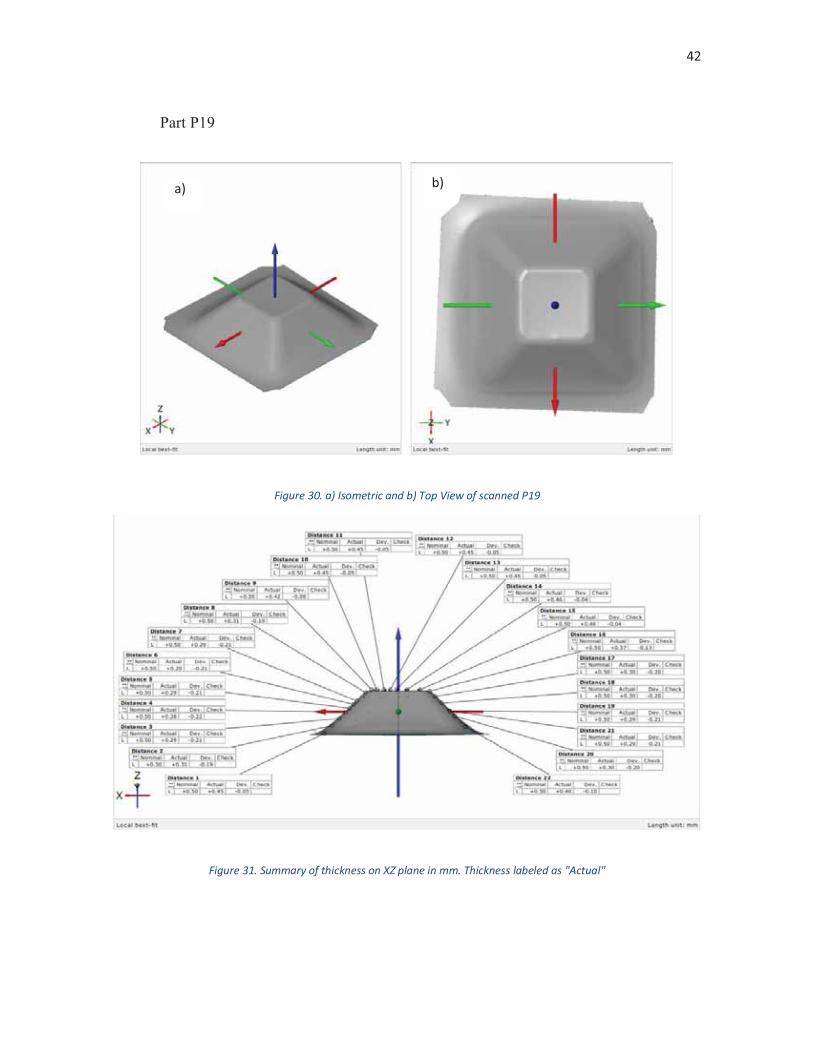
Part P19
Figure 30. a) Isometric and b) Top View of scanned P19
Figure 31. Summary of thickness on XZ plane in mm. Thickness labeled as "Actual"
b) a)
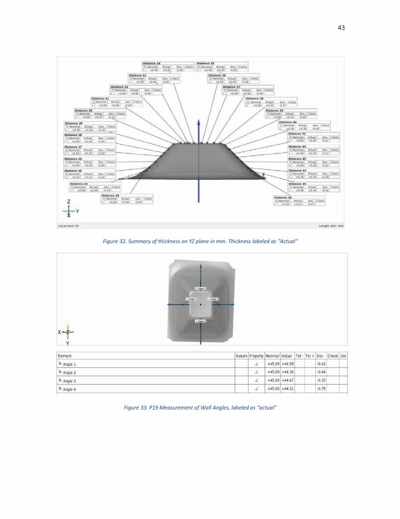
43
Figure 32. Summary of thickness on YZ plane in mm. Thickness labeled as "Actual"
Figure 33. P19 Measurement of Wall Angles, labeled as “actual”
44
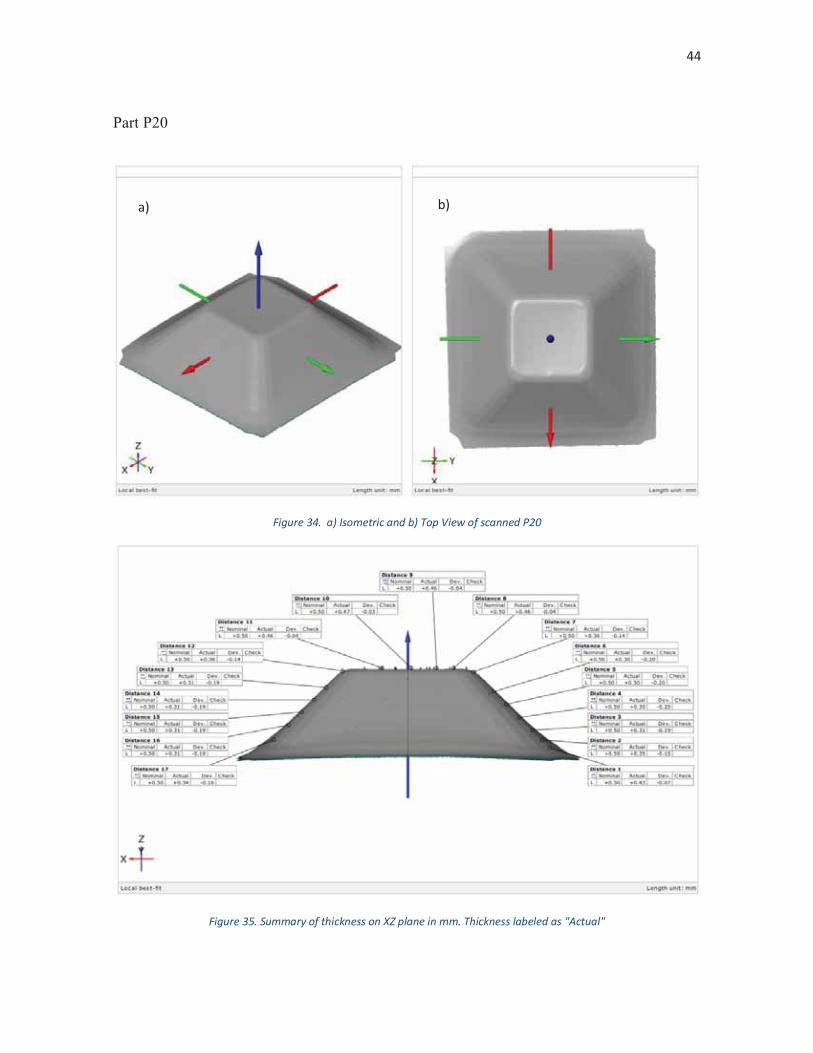
Part P20
Figure 34. a) Isometric and b) Top View of scanned P20
Figure 35. Summary of thickness on XZ plane in mm. Thickness labeled as "Actual"
a) b)
45
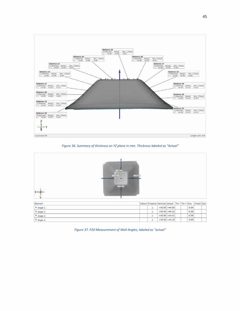
Figure 36. Summary of thickness on YZ plane in mm. Thickness labeled as "Actual"
Figure 37. P20 Measurement of Wall Angles, labeled as “actual”
46
Part P21
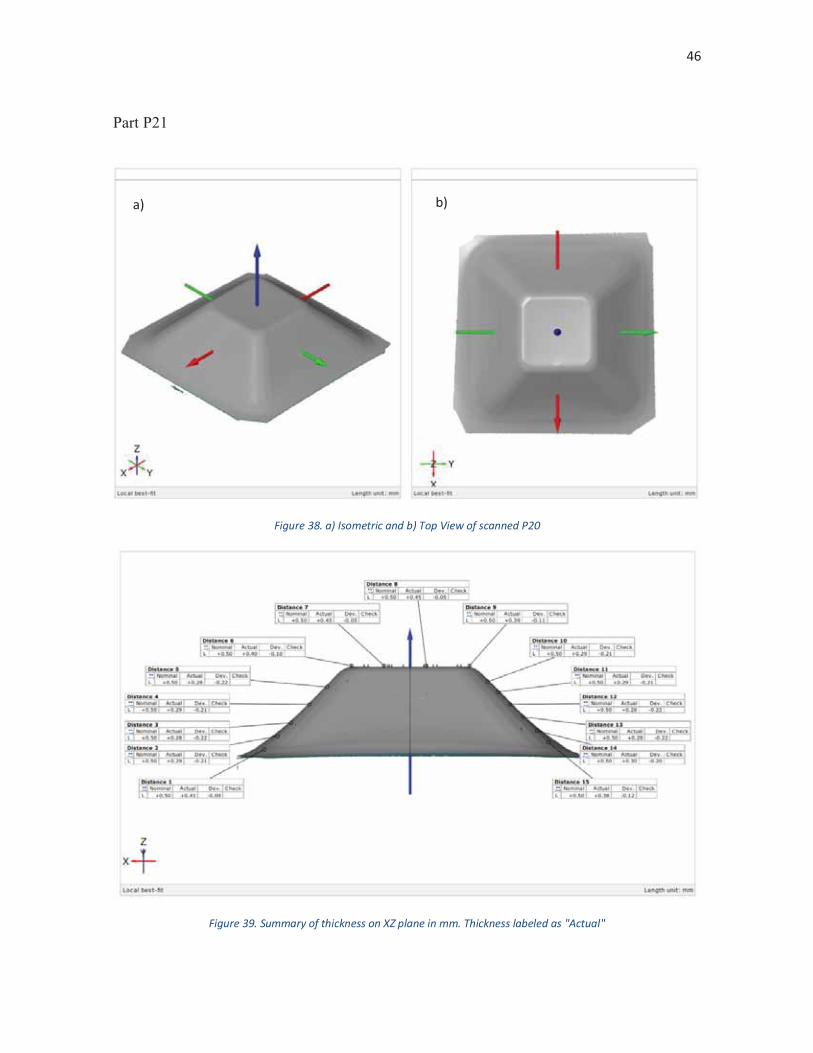
Figure 38. a) Isometric and b) Top View of scanned P20
Figure 39. Summary of thickness on XZ plane in mm. Thickness labeled as "Actual"
a) b)
47
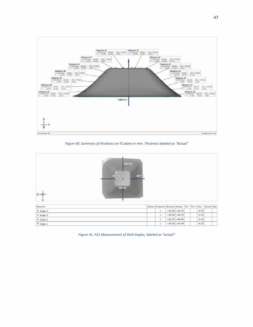
Figure 40. Summary of thickness on YZ plane in mm. Thickness labeled as "Actual"
Figure 41. P21 Measurement of Wall Angles, labeled as “actual”
48
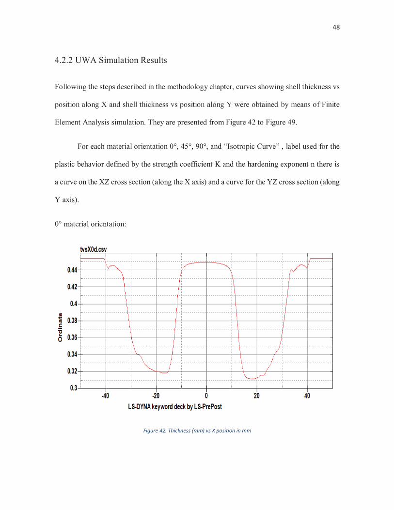
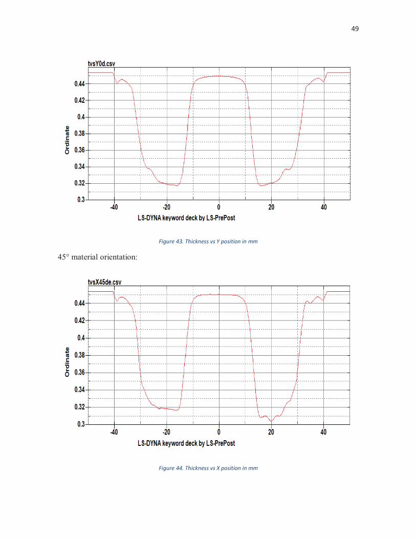
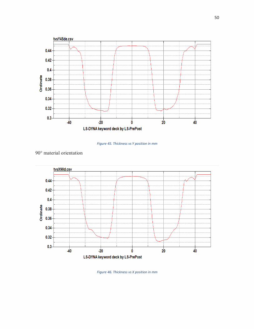
4.2.2 UWA Simulation Results
Following the steps described in the methodology chapter, curves showing shell thickness vs
position along X and shell thickness vs position along Y were obtained by means of Finite
Element Analysis simulation. They are presented from Figure 42 to Figure 49.
For each material orientation 0°, 45°, 90°, and “Isotropic Curve” , label used for the
plastic behavior defined by the strength coefficient K and the hardening exponent n there is
a curve on the XZ cross section (along the X axis) and a curve for the YZ cross section (along
Y axis).
0° material orientation:
Figure 42. Thickness (mm) vs X position in mm
49
Figure 43. Thickness vs Y position in mm
45° material orientation:
Figure 44. Thickness vs X position in mm
50
Figure 45. Thickness vs Y position in mm
90° material orientation
Figure 46. Thickness vs X position in mm
51
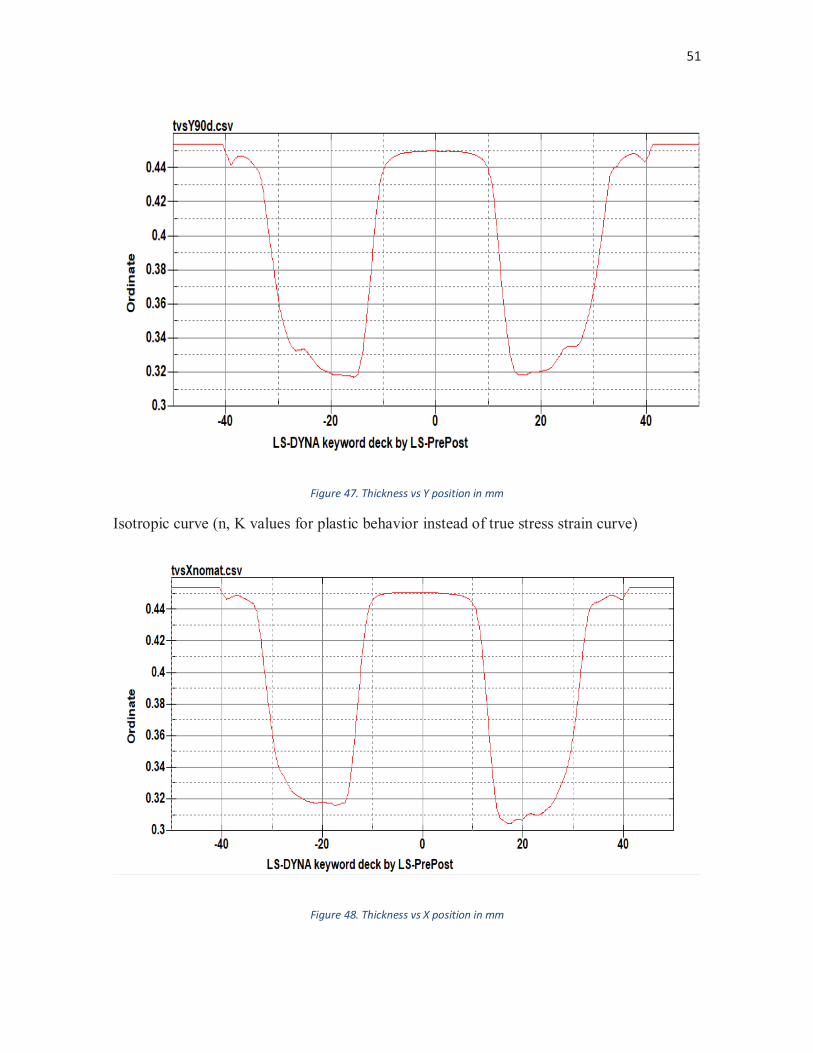
Figure 47. Thickness vs Y position in mm
Isotropic curve (n, K values for plastic behavior instead of true stress strain curve)
Figure 48. Thickness vs X position in mm
52
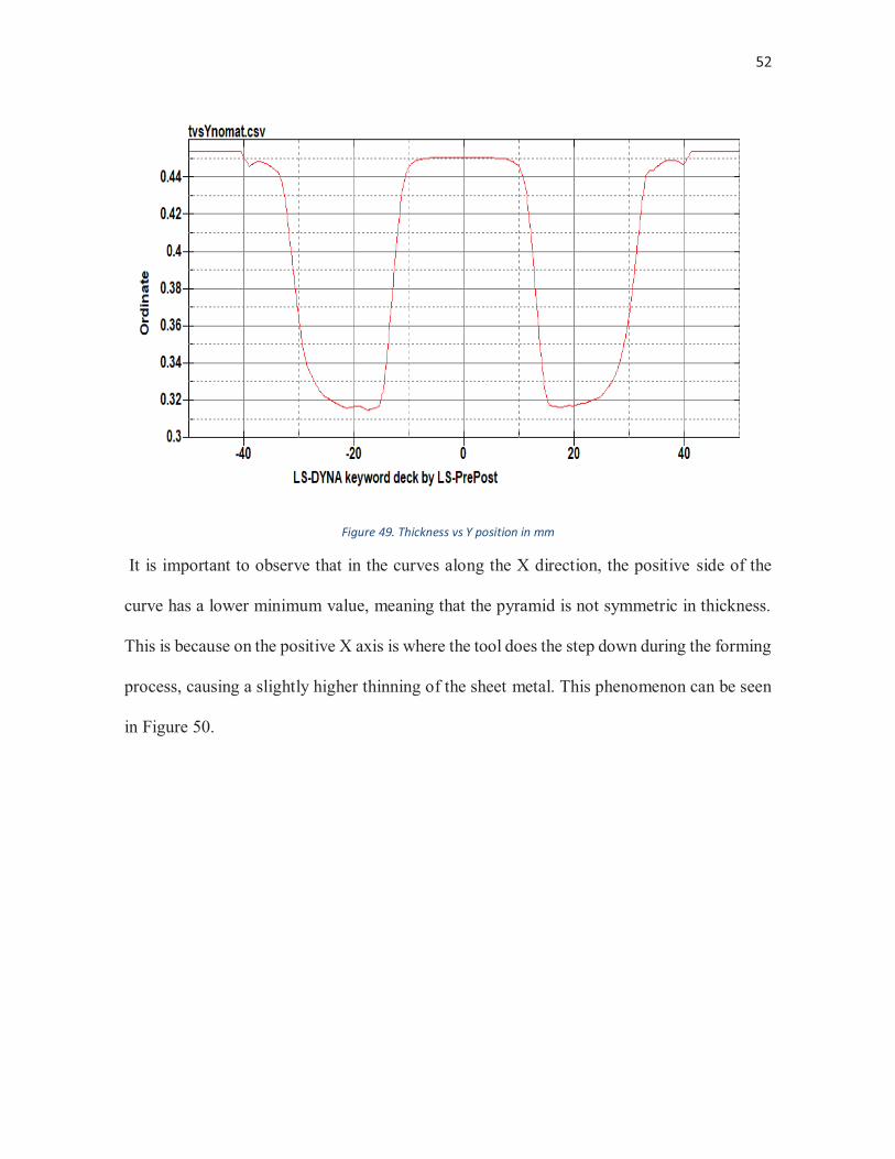
Figure 49. Thickness vs Y position in mm
It is important to observe that in the curves along the X direction, the positive side of the
curve has a lower minimum value, meaning that the pyramid is not symmetric in thickness.
This is because on the positive X axis is where the tool does the step down during the forming
process, causing a slightly higher thinning of the sheet metal. This phenomenon can be seen
in Figure 50.
53
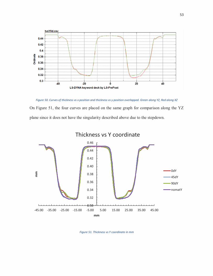
Figure 50. Curves of thickness vs x position and thickness vs y position overlapped. Green along YZ, Red along XZ
On Figure 51, the four curves are placed on the same graph for comparison along the YZ
plane since it does not have the singularity described above due to the stepdown.
Figure 51. Thickness vs Y coordinate in mm
0.30
0.32
0.34
0.36
0.38
0.40
0.42
0.44
0.46
-45.00 -35.00 -25.00 -15.00 -5.00 5.00 15.00 25.00 35.00 45.00
mm
mm
Thickness vs Y coordinate
0dY
45dY
90dY
nomatY
54
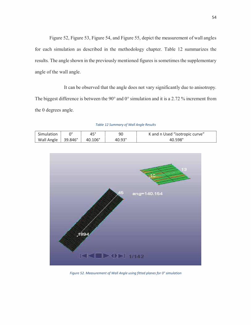
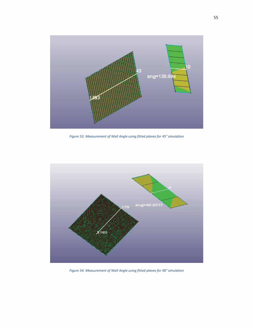
Figure 52, Figure 53, Figure 54, and Figure 55, depict the measurement of wall angles
for each simulation as described in the methodology chapter. Table 12 summarizes the
results. The angle shown in the previously mentioned figures is sometimes the supplementary
angle of the wall angle.
It can be observed that the angle does not vary significantly due to anisotropy.
The biggest difference is between the 90° and 0° simulation and it is a 2.72 % increment from
the 0 degrees angle.
Table 12 Summary of Wall Angle Results
Simulation 0° 45° 90 K and n Used “isotropic curve” Wall Angle 39.846° 40.106° 40.93° 40.598°
Figure 52. Measurement of Wall Angle using fitted planes for 0° simulation
55
Figure 53. Measurement of Wall Angle using fitted planes for 45° simulation
Figure 54. Measurement of Wall Angle using fitted planes for 90° simulation
56
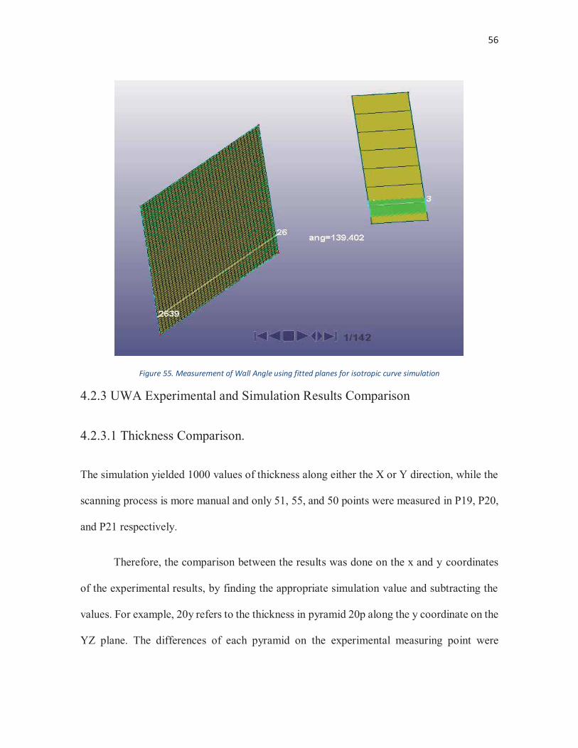
Figure 55. Measurement of Wall Angle using fitted planes for isotropic curve simulation
4.2.3 UWA Experimental and Simulation Results Comparison
4.2.3.1 Thickness Comparison.
The simulation yielded 1000 values of thickness along either the X or Y direction, while the
scanning process is more manual and only 51, 55, and 50 points were measured in P19, P20,
and P21 respectively.
Therefore, the comparison between the results was done on the x and y coordinates
of the experimental results, by finding the appropriate simulation value and subtracting the
values. For example, 20y refers to the thickness in pyramid 20p along the y coordinate on the
YZ plane. The differences of each pyramid on the experimental measuring point were
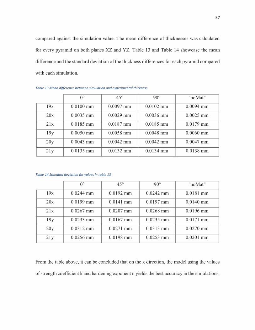
57
compared against the simulation value. The mean difference of thicknesses was calculated
for every pyramid on both planes XZ and YZ. Table 13 and Table 14 showcase the mean
difference and the standard deviation of the thickness differences for each pyramid compared
with each simulation.
Table 13 Mean difference between simulation and experimental thickness.
0° 45° 90° "noMat"
19x 0.0100 mm 0.0097 mm 0.0102 mm 0.0094 mm
20x 0.0035 mm 0.0029 mm 0.0036 mm 0.0025 mm
21x 0.0185 mm 0.0187 mm 0.0185 mm 0.0179 mm
19y 0.0050 mm 0.0058 mm 0.0048 mm 0.0060 mm
20y 0.0043 mm 0.0042 mm 0.0042 mm 0.0047 mm
21y 0.0135 mm 0.0132 mm 0.0134 mm 0.0138 mm
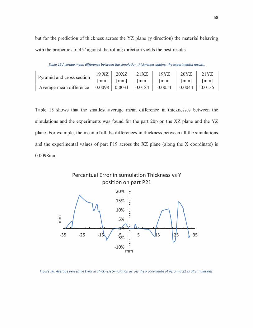
Table 14 Standard deviation for values in table 13.
0° 45° 90° "noMat"
19x 0.0244 mm 0.0192 mm 0.0242 mm 0.0181 mm
20x 0.0199 mm 0.0141 mm 0.0197 mm 0.0140 mm
21x 0.0267 mm 0.0207 mm 0.0268 mm 0.0196 mm
19y 0.0233 mm 0.0167 mm 0.0235 mm 0.0171 mm
20y 0.0312 mm 0.0271 mm 0.0313 mm 0.0270 mm
21y 0.0256 mm 0.0198 mm 0.0253 mm 0.0201 mm
From the table above, it can be concluded that on the x direction, the model using the values
of strength coefficient k and hardening exponent n yields the best accuracy in the simulations,
58
but for the prediction of thickness across the YZ plane (y direction) the material behaving
with the properties of 45° against the rolling direction yields the best results.
Table 15 Average mean difference between the simulation thicknesses against the experimental results.
Pyramid and cross section 19 XZ [mm]
20XZ [mm]
21XZ [mm]
19YZ [mm]
20YZ [mm]
21YZ [mm]
Average mean difference 0.0098 0.0031 0.0184 0.0054 0.0044 0.0135
Table 15 shows that the smallest average mean difference in thicknesses between the
simulations and the experiments was found for the part 20p on the XZ plane and the YZ
plane. For example, the mean of all the differences in thickness between all the simulations
and the experimental values of part P19 across the XZ plane (along the X coordinate) is
0.0098mm.
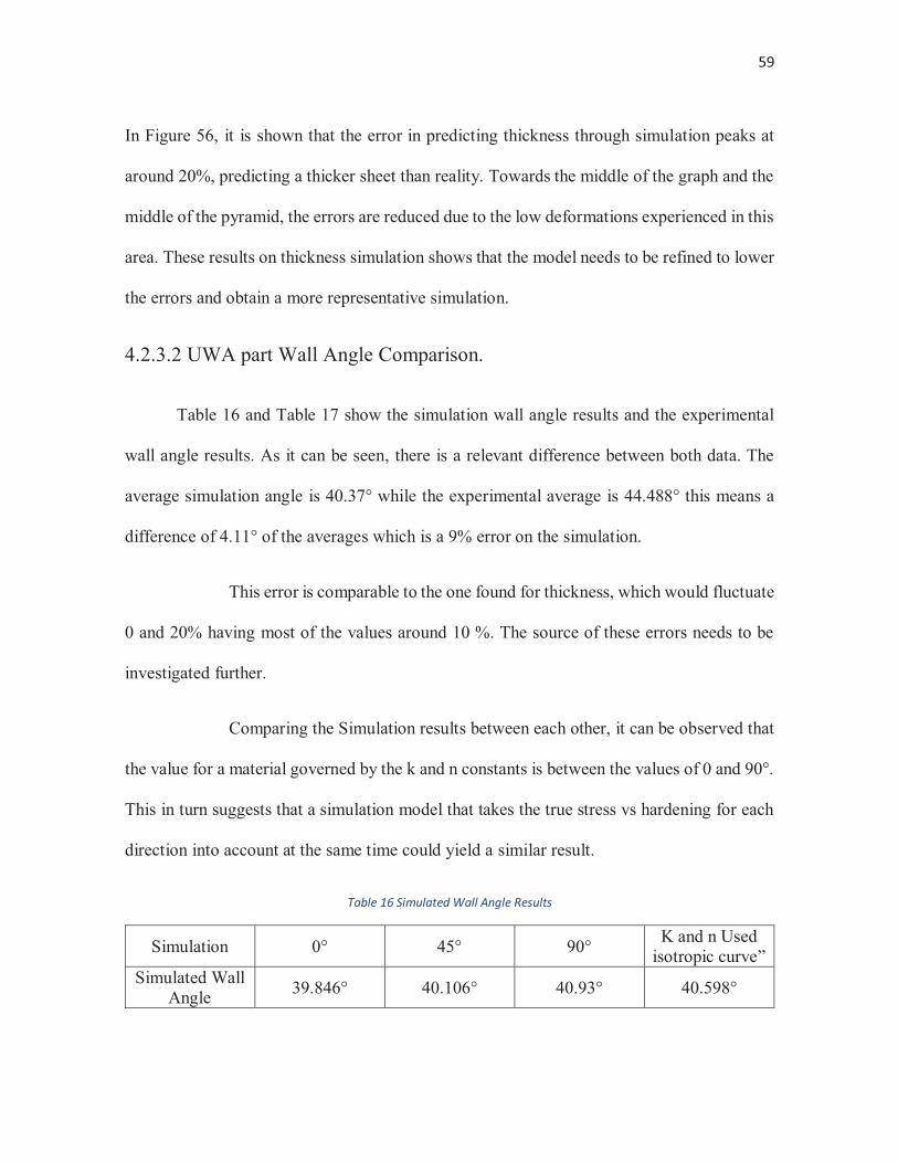
Figure 56. Average percentile Error in Thickness Simulation across the y coordinate of pyramid 21 vs all simulations.
-10%
-5%
0%
5%
10%
15%
20%
-35 -25 -15 -5 5 15 25 35
mm
mm
Percentual Error in sumulation Thickness vs Y position on part P21
59
In Figure 56, it is shown that the error in predicting thickness through simulation peaks at
around 20%, predicting a thicker sheet than reality. Towards the middle of the graph and the
middle of the pyramid, the errors are reduced due to the low deformations experienced in this
area. These results on thickness simulation shows that the model needs to be refined to lower
the errors and obtain a more representative simulation.
4.2.3.2 UWA part Wall Angle Comparison.
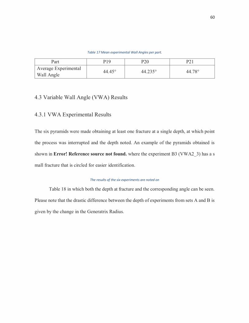
Table 16 and Table 17 show the simulation wall angle results and the experimental
wall angle results. As it can be seen, there is a relevant difference between both data. The
average simulation angle is 40.37° while the experimental average is 44.488° this means a
difference of 4.11° of the averages which is a 9% error on the simulation.
This error is comparable to the one found for thickness, which would fluctuate
0 and 20% having most of the values around 10 %. The source of these errors needs to be
investigated further.
Comparing the Simulation results between each other, it can be observed that
the value for a material governed by the k and n constants is between the values of 0 and 90°.
This in turn suggests that a simulation model that takes the true stress vs hardening for each
direction into account at the same time could yield a similar result.
Table 16 Simulated Wall Angle Results
Simulation 0° 45° 90° K and n Used isotropic curve”
Simulated Wall Angle 39.846° 40.106° 40.93° 40.598°
60
Table 17 Mean experimental Wall Angles per part.
Part P19 P20 P21 Average Experimental Wall Angle
44.45° 44.235° 44.78°
4.3 Variable Wall Angle (VWA) Results
4.3.1 VWA Experimental Results
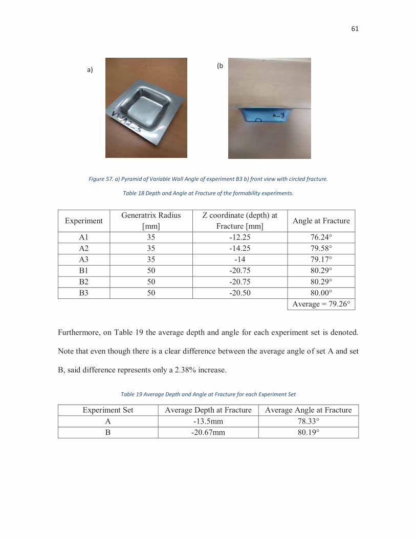
The six pyramids were made obtaining at least one fracture at a single depth, at which point
the process was interrupted and the depth noted. An example of the pyramids obtained is
shown in Error! Reference source not found. where the experiment B3 (VWA2_3) has a s
mall fracture that is circled for easier identification.
The results of the six experiments are noted on
Table 18 in which both the depth at fracture and the corresponding angle can be seen.
Please note that the drastic difference between the depth of experiments from sets A and B is
given by the change in the Generatrix Radius.
61
Figure 57. a) Pyramid of Variable Wall Angle of experiment B3 b) front view with circled fracture.
Table 18 Depth and Angle at Fracture of the formability experiments.
Furthermore, on Table 19 the average depth and angle for each experiment set is denoted.
Note that even though there is a clear difference between the average angle of set A and set
B, said difference represents only a 2.38% increase.
Table 19 Average Depth and Angle at Fracture for each Experiment Set
Experiment Set Average Depth at Fracture Average Angle at Fracture A -13.5mm 78.33° B -20.67mm 80.19°
Experiment Generatrix Radius
[mm] Z coordinate (depth) at
Fracture [mm] Angle at Fracture
A1 35 -12.25 76.24° A2 35 -14.25 79.58° A3 35 -14 79.17° B1 50 -20.75 80.29° B2 50 -20.75 80.29° B3 50 -20.50 80.00°
Average = 79.26°
a) (b
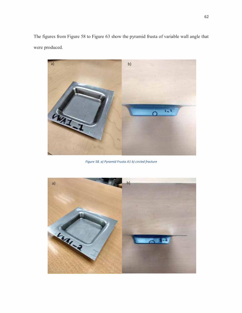
62
The figures from Figure 58 to Figure 63 show the pyramid frusta of variable wall angle that
were produced.
Figure 58. a) Pyramid Frusta A1 b) circled fracture
b) a)
b) a)
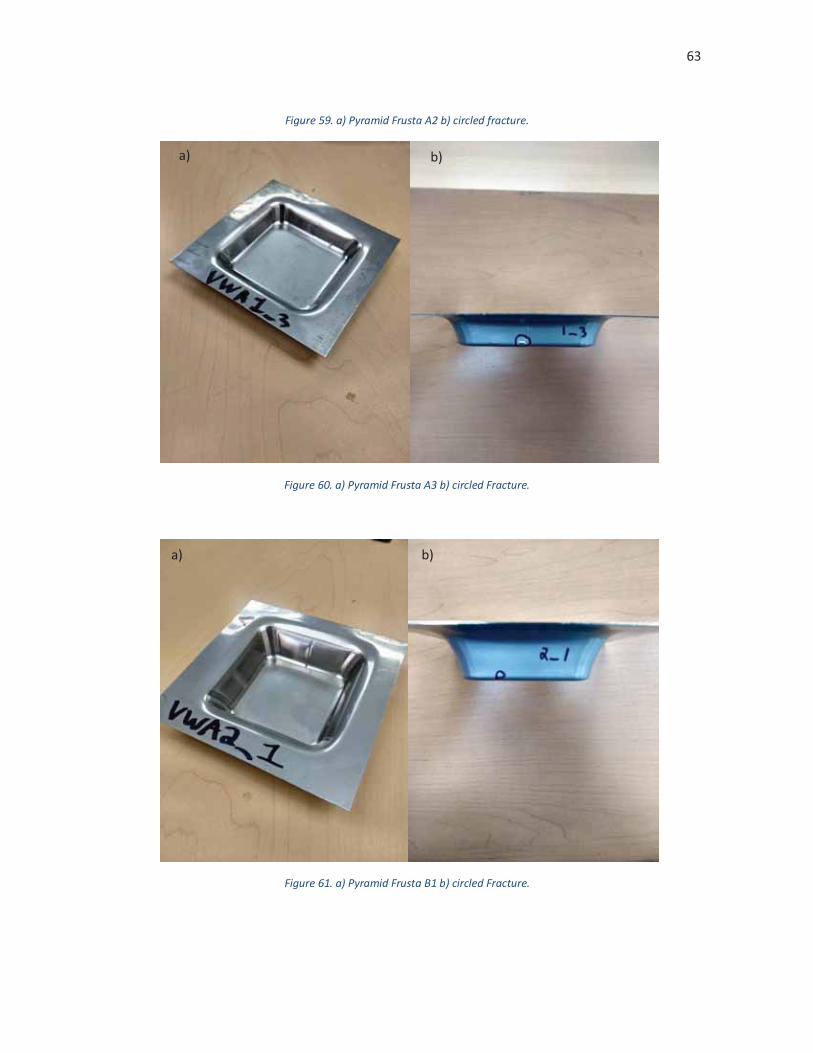
63
Figure 59. a) Pyramid Frusta A2 b) circled fracture.
Figure 60. a) Pyramid Frusta A3 b) circled Fracture.
Figure 61. a) Pyramid Frusta B1 b) circled Fracture.
b) a)
a) b)
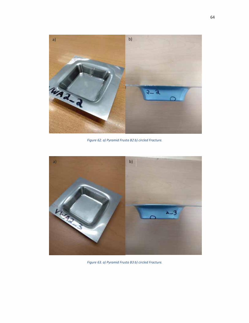
64
Figure 62. a) Pyramid Frusta B2 b) circled Fracture.
a) b)
b) a)
Figure 63. a) Pyramid Frusta B3 b) circled Fracture.
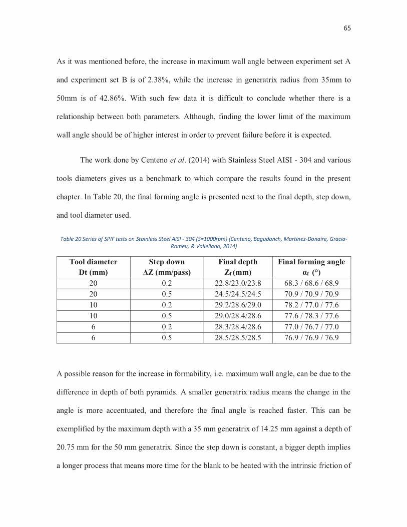
65
As it was mentioned before, the increase in maximum wall angle between experiment set A
and experiment set B is of 2.38%, while the increase in generatrix radius from 35mm to
50mm is of 42.86%. With such few data it is difficult to conclude whether there is a
relationship between both parameters. Although, finding the lower limit of the maximum
wall angle should be of higher interest in order to prevent failure before it is expected.
The work done by Centeno et al. (2014) with Stainless Steel AISI - 304 and various
tools diameters gives us a benchmark to which compare the results found in the present
chapter. In Table 20, the final forming angle is presented next to the final depth, step down,
and tool diameter used.
Table 20 Series of SPIF tests on Stainless Steel AISI - 304 (S=1000rpm) (Centeno, Bagudanch, Martinez-Donaire, Gracia-Romeu, & Vallellano, 2014)
Tool diameter Dt (mm)
Step down ΔZ (mm/pass)
Final depth Zf (mm)
Final forming angle αf (°)
20 0.2 22.8/23.0/23.8 68.3 / 68.6 / 68.9 20 0.5 24.5/24.5/24.5 70.9 / 70.9 / 70.9 10 0.2 29.2/28.6/29.0 78.2 / 77.0 / 77.6 10 0.5 29.0/28.4/28.6 77.6 / 78.3 / 77.6 6 0.2 28.3/28.4/28.6 77.0 / 76.7 / 77.0 6 0.5 28.5/28.5/28.5 76.9 / 76.9 / 76.9
A possible reason for the increase in formability, i.e. maximum wall angle, can be due to the
difference in depth of both pyramids. A smaller generatrix radius means the change in the
angle is more accentuated, and therefore the final angle is reached faster. This can be
exemplified by the maximum depth with a 35 mm generatrix of 14.25 mm against a depth of
20.75 mm for the 50 mm generatrix. Since the step down is constant, a bigger depth implies
a longer process that means more time for the blank to be heated with the intrinsic friction of
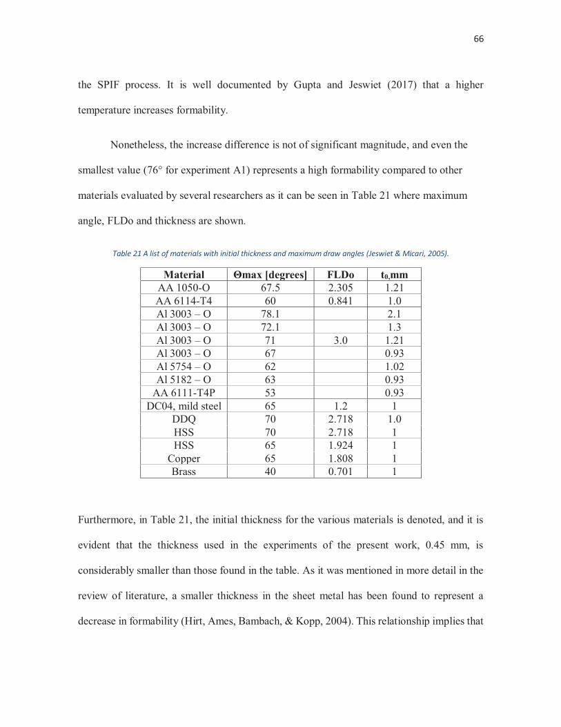
66
the SPIF process. It is well documented by Gupta and Jeswiet (2017) that a higher
temperature increases formability.
Nonetheless, the increase difference is not of significant magnitude, and even the
smallest value (76° for experiment A1) represents a high formability compared to other
materials evaluated by several researchers as it can be seen in Table 21 where maximum
angle, FLDo and thickness are shown.
Table 21 A list of materials with initial thickness and maximum draw angles (Jeswiet & Micari, 2005).
Material Θmax [degrees] FLDo t0,mm AA 1050-O 67.5 2.305 1.21 AA 6114-T4 60 0.841 1.0 Al 3003 – O 78.1 2.1 Al 3003 – O 72.1 1.3 Al 3003 – O 71 3.0 1.21 Al 3003 – O 67 0.93 Al 5754 – O 62 1.02 Al 5182 – O 63 0.93
AA 6111-T4P 53 0.93 DC04, mild steel 65 1.2 1
DDQ 70 2.718 1.0 HSS 70 2.718 1 HSS 65 1.924 1
Copper 65 1.808 1 Brass 40 0.701 1
Furthermore, in Table 21, the initial thickness for the various materials is denoted, and it is
evident that the thickness used in the experiments of the present work, 0.45 mm, is
considerably smaller than those found in the table. As it was mentioned in more detail in the
review of literature, a smaller thickness in the sheet metal has been found to represent a
decrease in formability (Hirt, Ames, Bambach, & Kopp, 2004). This relationship implies that
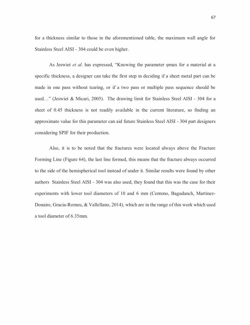
67
for a thickness similar to those in the aforementioned table, the maximum wall angle for
Stainless Steel AISI - 304 could be even higher.
As Jeswiet et al. has expressed, “Knowing the parameter φmax for a material at a
specific thickness, a designer can take the first step in deciding if a sheet metal part can be
made in one pass without tearing, or if a two pass or multiple pass sequence should be
used…” (Jeswiet & Micari, 2005). The drawing limit for Stainless Steel AISI - 304 for a
sheet of 0.45 thickness is not readily available in the current literature, so finding an
approximate value for this parameter can aid future Stainless Steel AISI - 304 part designers
considering SPIF for their production.
Also, it is to be noted that the fractures were located always above the Fracture
Forming Line (Figure 64), the last line formed, this means that the fracture always occurred
to the side of the hemispherical tool instead of under it. Similar results were found by other
authors Stainless Steel AISI - 304 was also used, they found that this was the case for their
experiments with lower tool diameters of 10 and 6 mm (Centeno, Bagudanch, Martinez-
Donaire, Gracia-Romeu, & Vallellano, 2014), which are in the range of this work which used
a tool diameter of 6.35mm.
68
Figure 64. Detail Image featuring the fracture of a VWA part
4.3.2 VWA Simulation Results
For Variable Wall Angle parts, the simulation was used to find the maximum effective strain
at which the fractures might have occurred. For a more detailed description of this process
refer to the methodology chapter.
A summary of the results is provided in Table 22 and in Table 23 for experiment set
A and B respectively. The effective plastic strain is taken from each simulation at the fracture
height, including the simulation for the material’s plastic behavior defined by the strength
coefficient k and hardening exponent n of Stainless Steel AISI - 304.
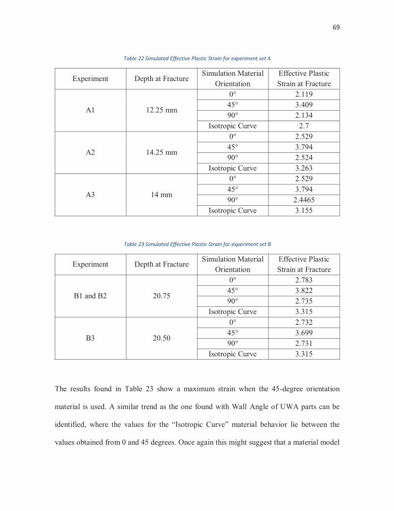
69
Table 22 Simulated Effective Plastic Strain for experiment set A
Experiment Depth at Fracture Simulation Material
Orientation Effective Plastic Strain at Fracture
A1 12.25 mm
0° 2.119 45° 3.409 90° 2.134
Isotropic Curve 2.7
A2 14.25 mm
0° 2.529 45° 3.794 90° 2.524
Isotropic Curve 3.263
A3 14 mm
0° 2.529 45° 3.794 90° 2.4465
Isotropic Curve 3.155
Table 23 Simulated Effective Plastic Strain for experiment set B
Experiment Depth at Fracture Simulation Material
Orientation Effective Plastic Strain at Fracture
B1 and B2 20.75
0° 2.783 45° 3.822 90° 2.735
Isotropic Curve 3.315
B3 20.50
0° 2.732 45° 3.699 90° 2.731
Isotropic Curve 3.315
The results found in Table 23 show a maximum strain when the 45-degree orientation
material is used. A similar trend as the one found with Wall Angle of UWA parts can be
identified, where the values for the “Isotropic Curve” material behavior lie between the
values obtained from 0 and 45 degrees. Once again this might suggest that a material model
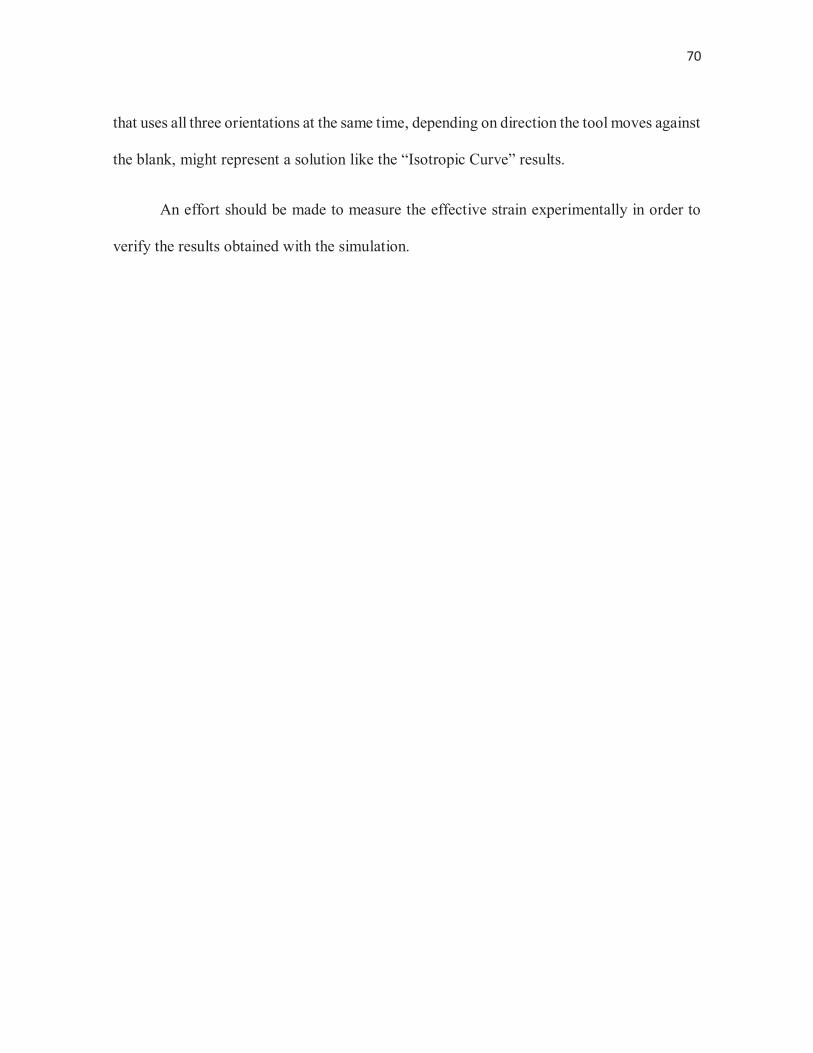
70
that uses all three orientations at the same time, depending on direction the tool moves against
the blank, might represent a solution like the “Isotropic Curve” results.
An effort should be made to measure the effective strain experimentally in order to
verify the results obtained with the simulation.
71
Chapter Five: Conclusions and Outlook
The results found in the present work provide some useful insight into forming Stainless Steel
AISI - 304 with Single Point Incremental Forming. An experimental formability limit was
found with a maximum wall angle of 79.26°. For the design of parts, it is recommended to
stay under 75° to stand clear of the found limit. Also, the sheet thinning according to the
Cosine’s law should be taken into account for future part design using this process.
Also, a clear effect of anisotropy was found on the effective plastic strain where 45°
from rolling direction was found to have the greatest value. The effects of anisotropy on the
wall thickness was also observed where again, at 45° from the rolling direction the results
were significantly different. This coincides with the research done on Aluminum by Kumar
et al. (2018), where the same direction was found to oppose deformation more than 0 and 90
degrees.
Finally, the effects of anisotropy on Wall Angle are not evident and seem non-
significant.
This research opens a lot of doors for further investigation. Although Digital Image
Correlation was attempted for the Tensile Tests, it was not successfully implemented. This
technique needs to be successfully developed at UDLAP since the software and equipment
necessary is available. This would provide further detail at the necking and strain
concentration zone during a tensile test. This information could benefit the prediction of
effective plastic strain using the FEM model greatly.
72
Also, further research could be done on the improvement of the FEM simulation
model by means of experimenting with adaptive or sectionalized meshing to increase the
accuracy. SPIF has very localized deformation so small element sizes is necessary, but a
balance with computational cost needs to be found for the context of UDLAP. Additionally,
the effects of springback should be modeled and simulated.
Furthermore, by having FEM material models for all three directions of anisotropy, a
new model that uses all three models in the same simulation depending on the direction of
deformation can be implemented. Inside the LS Pre-Post software the material configuration
is called “Mat_3_Parameter_Barlat” and is the material 36. This line of research is already
being worked on by the author of the present work.
On the grounds of formability, experimental measurements of variable wall angle
parts should be conducted to obtain the major and minor strains around fracture points. This
way a maximum major strain at zero minor strain (FLDo) can be defined and compared with
the simulation results.
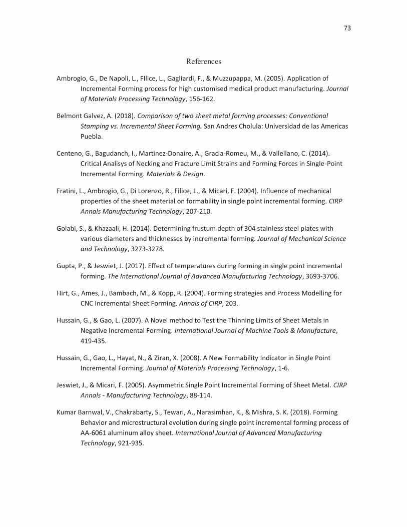
73
References
Ambrogio, G., De Napoli, L., FIlice, L., Gagliardi, F., & Muzzupappa, M. (2005). Application of Incremental Forming process for high customised medical product manufacturing. Journal of Materials Processing Technology, 156-162.
Belmont Galvez, A. (2018). Comparison of two sheet metal forming processes: Conventional Stamping vs. Incremental Sheet Forming. San Andres Cholula: Universidad de las Americas Puebla.
Centeno, G., Bagudanch, I., Martinez-Donaire, A., Gracia-Romeu, M., & Vallellano, C. (2014). Critical Analisys of Necking and Fracture Limit Strains and Forming Forces in Single-Point Incremental Forming. Materials & Design.
Fratini, L., Ambrogio, G., Di Lorenzo, R., Filice, L., & Micari, F. (2004). Influence of mechanical properties of the sheet material on formability in single point incremental forming. CIRP Annals Manufacturing Technology, 207-210.
Golabi, S., & Khazaali, H. (2014). Determining frustum depth of 304 stainless steel plates with various diameters and thicknesses by incremental forming. Journal of Mechanical Science and Technology, 3273-3278.
Gupta, P., & Jeswiet, J. (2017). Effect of temperatures during forming in single point incremental forming. The International Journal of Advanced Manufacturing Technology, 3693-3706.
Hirt, G., Ames, J., Bambach, M., & Kopp, R. (2004). Forming strategies and Process Modelling for CNC Incremental Sheet Forming. Annals of CIRP, 203.
Hussain, G., & Gao, L. (2007). A Novel method to Test the Thinning Limits of Sheet Metals in Negative Incremental Forming. International Journal of Machine Tools & Manufacture, 419-435.
Hussain, G., Gao, L., Hayat, N., & Ziran, X. (2008). A New Formability Indicator in Single Point Incremental Forming. Journal of Materials Processing Technology, 1-6.
Jeswiet, J., & Micari, F. (2005). Asymmetric Single Point Incremental Forming of Sheet Metal. CIRP Annals - Manufacturing Technology, 88-114.
Kumar Barnwal, V., Chakrabarty, S., Tewari, A., Narasimhan, K., & Mishra, S. K. (2018). Forming Behavior and microstructural evolution during single point incremental forming process of AA-6061 aluminum alloy sheet. International Journal of Advanced Manufacturing Technology, 921-935.
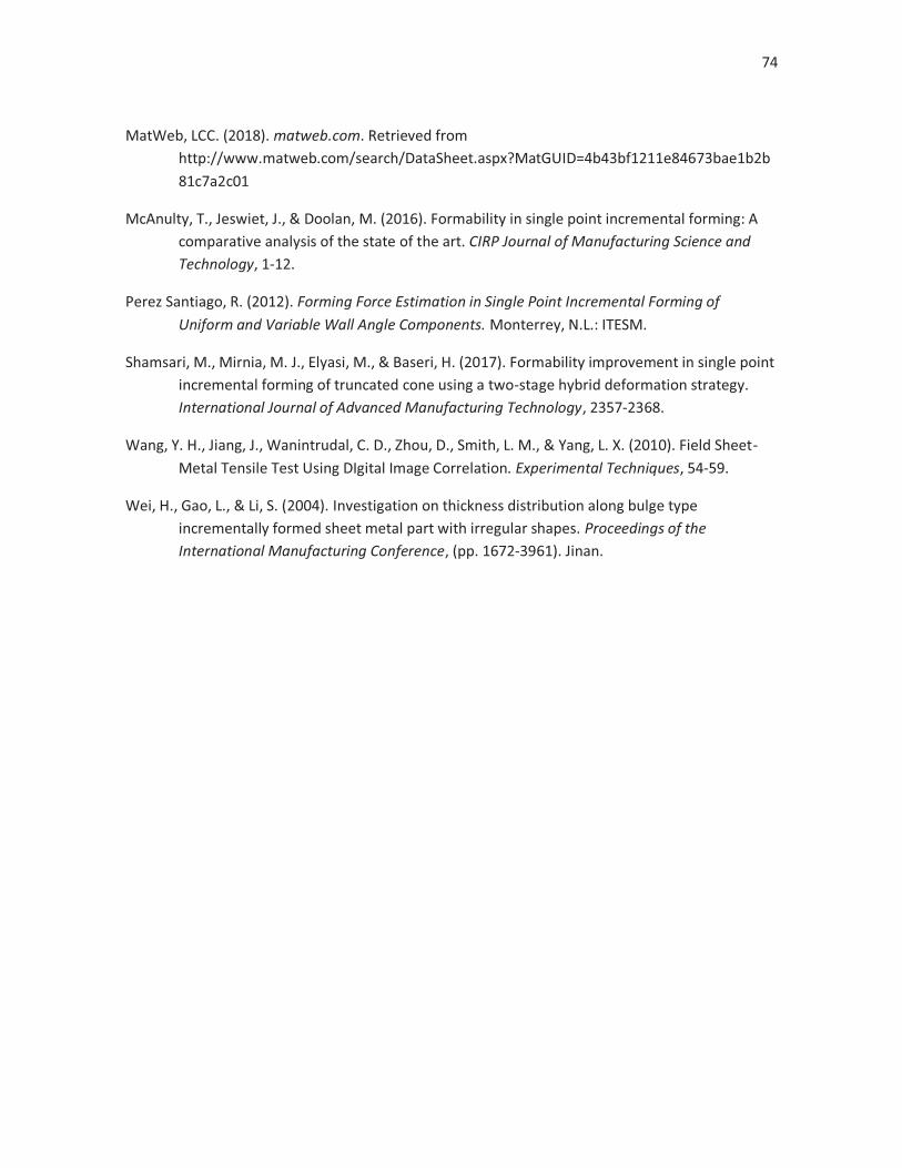
74
MatWeb, LCC. (2018). matweb.com. Retrieved from http://www.matweb.com/search/DataSheet.aspx?MatGUID=4b43bf1211e84673bae1b2b81c7a2c01
McAnulty, T., Jeswiet, J., & Doolan, M. (2016). Formability in single point incremental forming: A comparative analysis of the state of the art. CIRP Journal of Manufacturing Science and Technology, 1-12.
Perez Santiago, R. (2012). Forming Force Estimation in Single Point Incremental Forming of Uniform and Variable Wall Angle Components. Monterrey, N.L.: ITESM.
Shamsari, M., Mirnia, M. J., Elyasi, M., & Baseri, H. (2017). Formability improvement in single point incremental forming of truncated cone using a two-stage hybrid deformation strategy. International Journal of Advanced Manufacturing Technology, 2357-2368.
Wang, Y. H., Jiang, J., Wanintrudal, C. D., Zhou, D., Smith, L. M., & Yang, L. X. (2010). Field Sheet-Metal Tensile Test Using DIgital Image Correlation. Experimental Techniques, 54-59.
Wei, H., Gao, L., & Li, S. (2004). Investigation on thickness distribution along bulge type incrementally formed sheet metal part with irregular shapes. Proceedings of the International Manufacturing Conference, (pp. 1672-3961). Jinan.
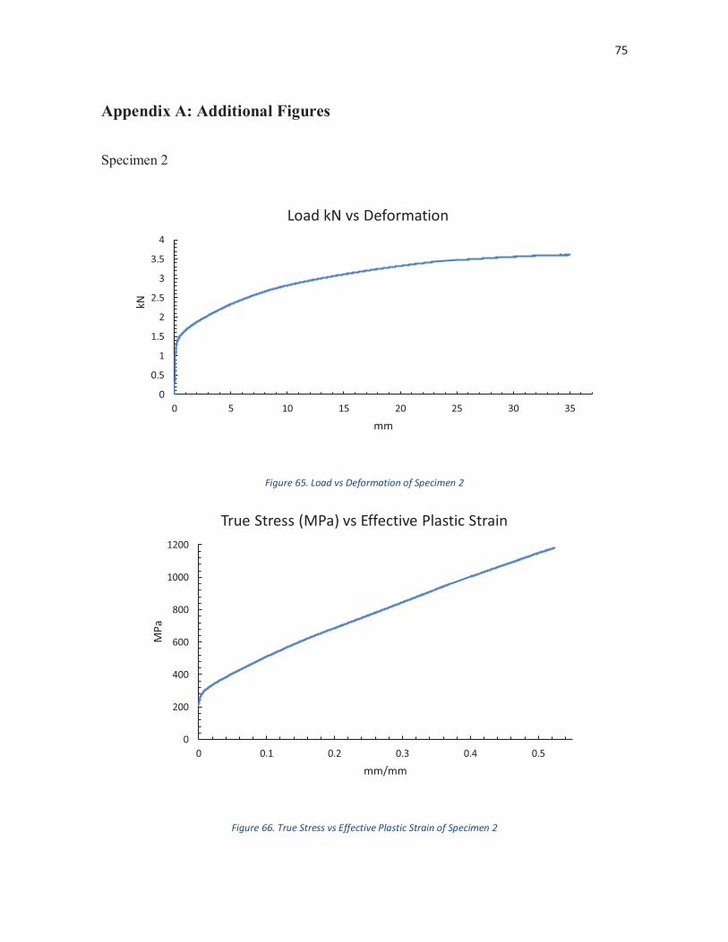
75
Appendix A: Additional Figures
Specimen 2
Figure 65. Load vs Deformation of Specimen 2
Figure 66. True Stress vs Effective Plastic Strain of Specimen 2
0
0.5
1
1.5
2
2.5
3
3.5
4
0 5 10 15 20 25 30 35
kN
mm
Load kN vs Deformation
0
200
400
600
800
1000
1200
0 0.1 0.2 0.3 0.4 0.5
MPa
mm/mm
True Stress (MPa) vs Effective Plastic Strain
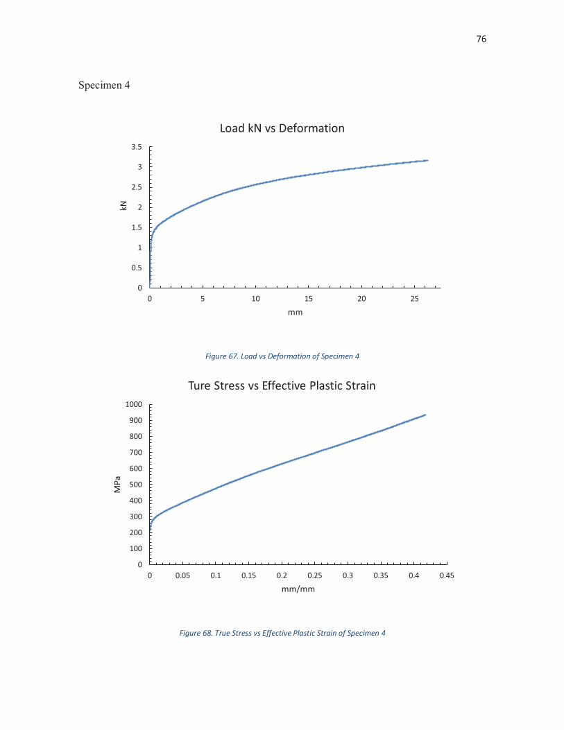
76
Specimen 4
Figure 67. Load vs Deformation of Specimen 4
Figure 68. True Stress vs Effective Plastic Strain of Specimen 4
0
0.5
1
1.5
2
2.5
3
3.5
0 5 10 15 20 25
kN
mm
Load kN vs Deformation
0
100
200
300
400
500
600
700
800
900
1000
0 0.05 0.1 0.15 0.2 0.25 0.3 0.35 0.4 0.45
MPa
mm/mm
Ture Stress vs Effective Plastic Strain
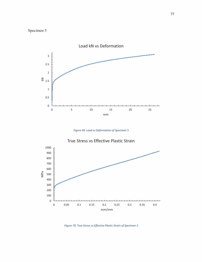
77
Specimen 5
Figure 69. Load vs Deformation of Specimen 5
Figure 70. True Stress vs Effective Plastic Strain of Specimen 5
0
0.5
1
1.5
2
2.5
3
0 5 10 15 20 25
kN
mm
Load kN vs Deformation
0
100
200
300
400
500
600
700
800
900
1000
0 0.05 0.1 0.15 0.2 0.25 0.3 0.35 0.4
MPa
mm/mm
True Stress vs Effective Plastic Strain
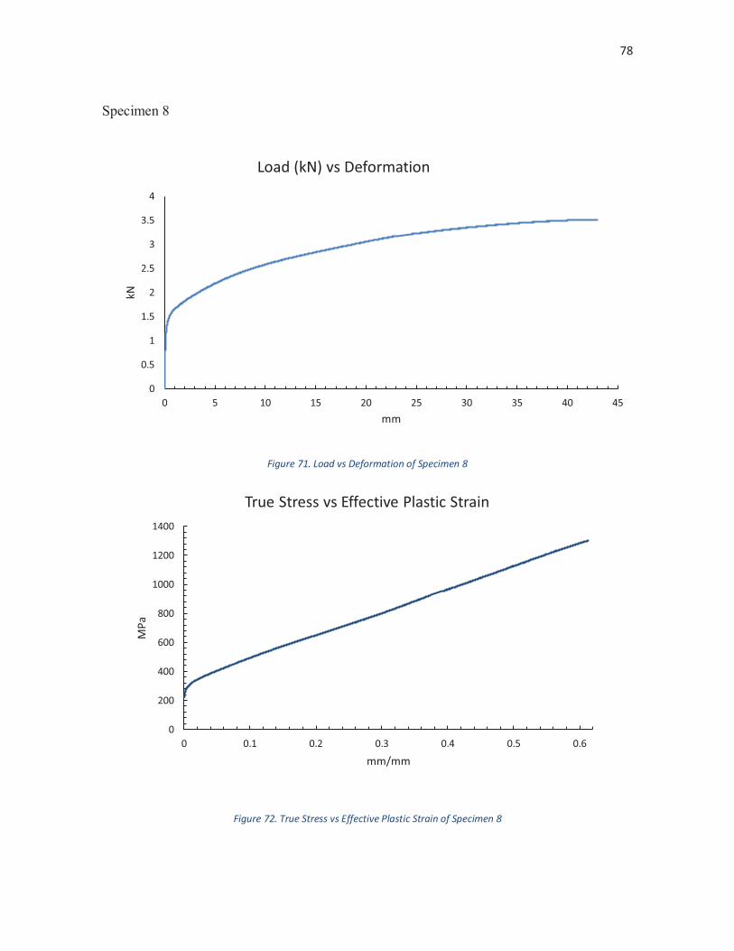
78
Specimen 8
Figure 71. Load vs Deformation of Specimen 8
Figure 72. True Stress vs Effective Plastic Strain of Specimen 8
0
0.5
1
1.5
2
2.5
3
3.5
4
0 5 10 15 20 25 30 35 40 45
kN
mm
Load (kN) vs Deformation
0
200
400
600
800
1000
1200
1400
0 0.1 0.2 0.3 0.4 0.5 0.6
MPa
mm/mm
True Stress vs Effective Plastic Strain
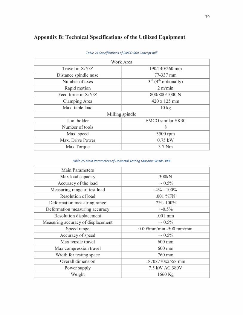
79
Appendix B: Technical Specifications of the Utilized Equipment
Table 24 Specifications of EMCO 500 Concept mill
Work Area Travel in X/Y/Z 190/140/260 mm
Distance spindle nose 77-337 mm Number of axes 3rd (4th optionally) Rapid motion 2 m/min
Feed force in X/Y/Z 800/800/1000 N Clamping Area 420 x 125 mm Max. table load 10 kg
Milling spindle Tool holder EMCO similar SK30
Number of tools 8 Max. speed 3500 rpm
Max. Drive Power 0.75 kW Max Torque 3.7 Nm
Table 25 Main Parameters of Universal Testing Machine WDW-300E
Main Parameters Max load capacity 300kN
Accuracy of the load +- 0.5% Measuring range of test load .4% - 100%
Resolution of load .001 %FN Deformation measuring range .2%- 100%
Deformation measuring accuracy +-0.5% Resolution displacement .001 mm
Measuring accuracy of displacement +- 0.5% Speed range 0.005mm/min -500 mm/min
Accuracy of speed +- 0.5% Max tensile travel 600 mm
Max compression travel 600 mm Width for testing space 760 mm
Overall dimension 1870x770x2558 mm Power supply 7.5 kW AC 380V
Weight 1660 Kg
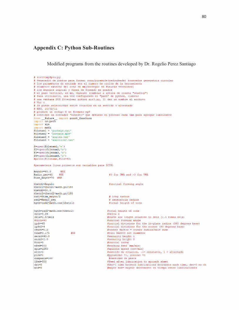
80
Appendix C: Python Sub-Routines
Modified programs from the routines developed by Dr. Rogelio Perez Santiago
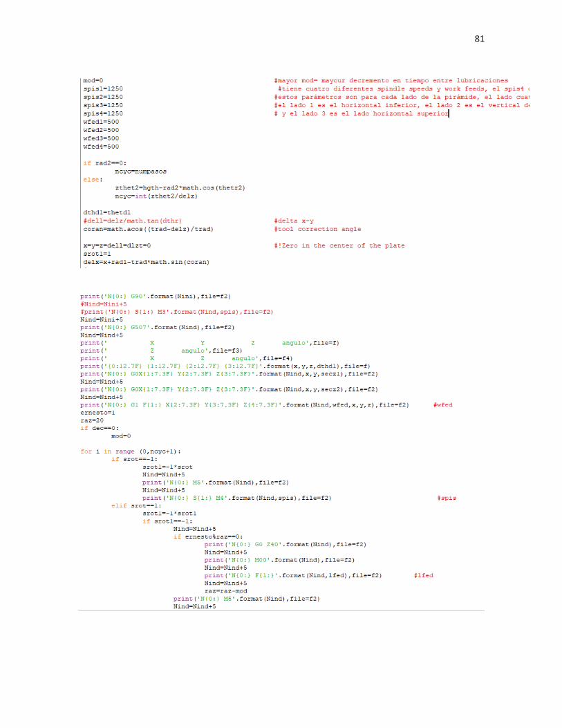
81
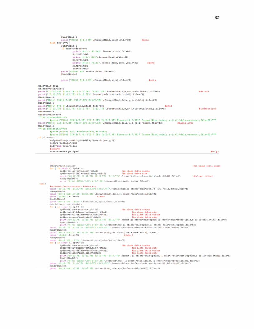
82
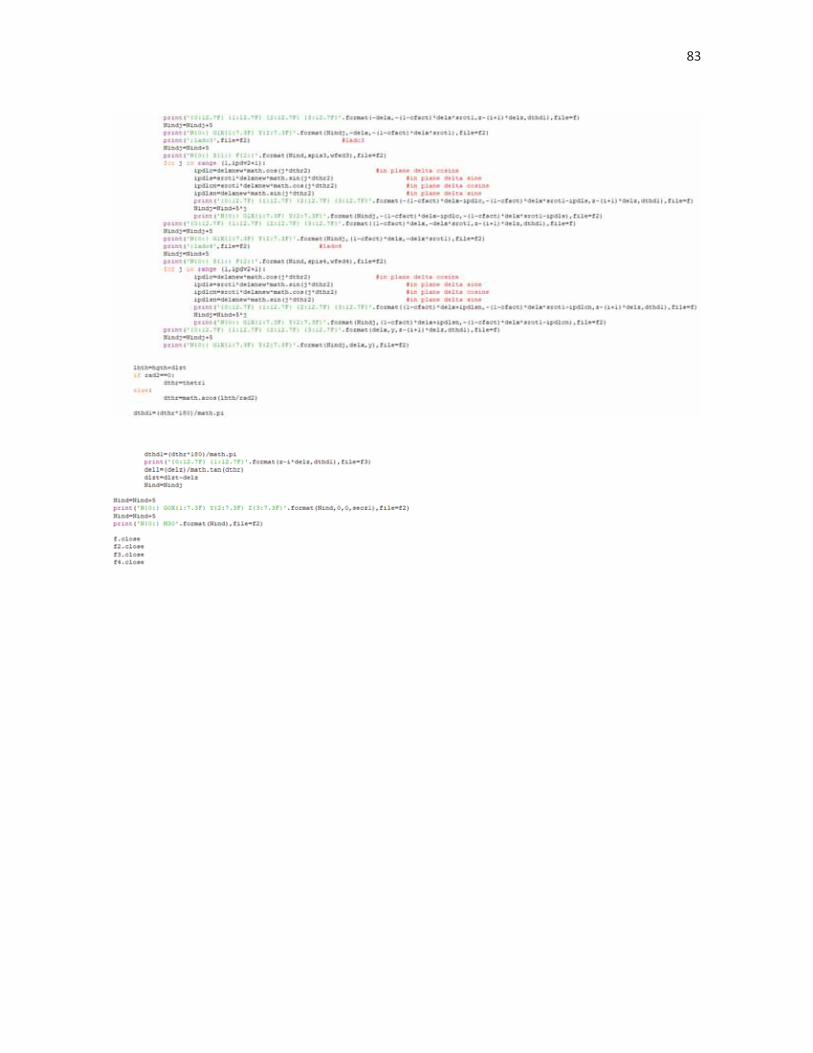
83
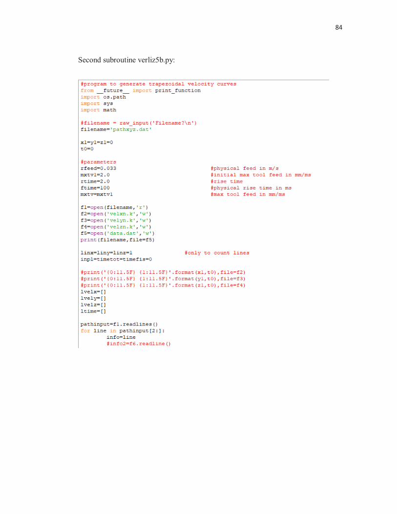
84
Second subroutine verliz5b.py:
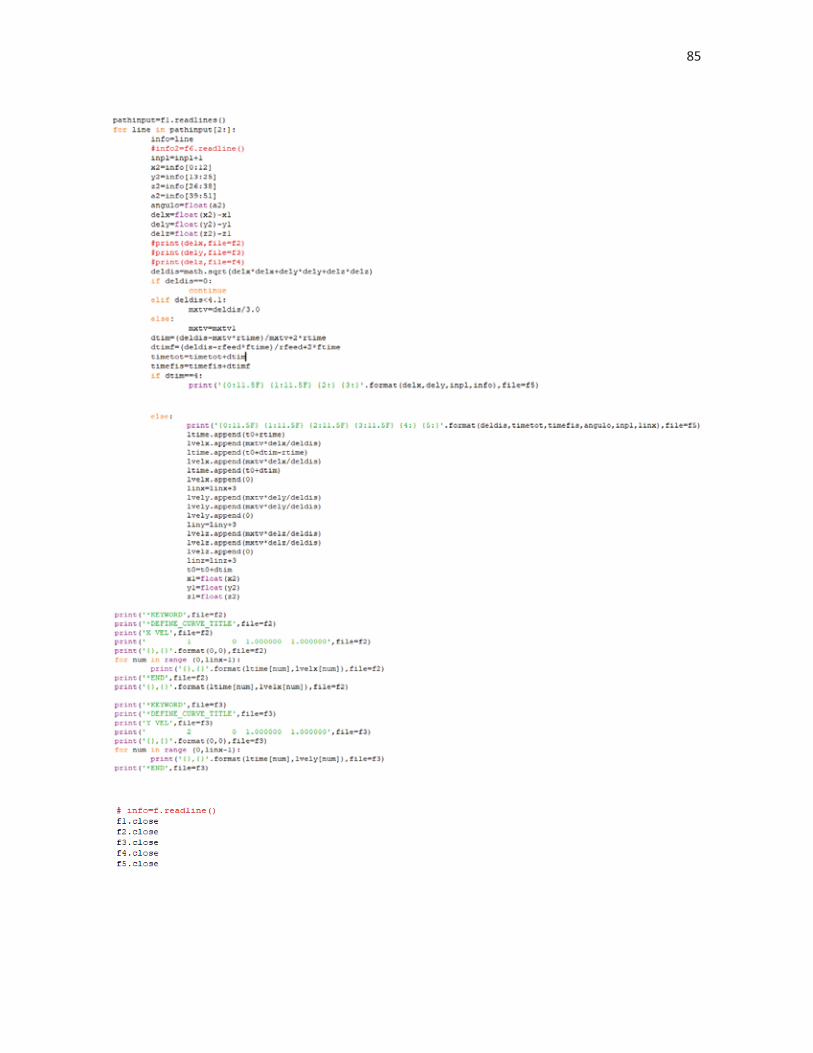
85