study on clustering techniques and application to...
TRANSCRIPT

Study On Clustering TechniquesAnd Application To Microarray
Gene Expression Bioinformatics Data
Kumar Dhiraj(Roll No: 60706001)
under the guidance of
Prof. Santanu Kumar Rath
Department of Computer Science and EngineeringNational Institute of Technology, Rourkela
Rourkela-769 008, Orissa, IndiaAugust, 2009.

Study On Clustering TechniquesAnd Application To Microarray
Gene Expression Bioinformatics Data
Thesis submitted in partial fulfillment
of the requirements for the degree of
Master of Technology(Research)
in
Computer Science and Engineering
by
Kumar Dhiraj(Roll No: 60706001)
Department of Computer Science and EngineeringNational Institute of Technology, Rourkela
Rourkela-769 008, Orissa, IndiaAugust, 2009.

Dedicated to my parents

Department of Computer Science and EngineeringNational Institute of Technology, RourkelaRourkela-769 008, Orissa, India.
Certificate
This is to certify that the work in the thesis entitled ” Study On Clustering Tech-
niques And Application To Microarray Gene Expression Bioinformatics Data” sub-
mitted by Kumar Dhiraj is a record of an original research work carried out by him
under my supervision and guidance in partial fulfillment of the requirements for the
award of the degree of Master of Technology (Research) in Computer Science and En-
gineering during the session 2007 – 2009 in the department of Computer Science and
Engineering, National Institute of Technology, Rourkela. Neither this thesis nor any
part of it has been submitted for any degree or academic award elsewhere.
Prof. Santanu Kumar Rath

Acknowledgment
First of all, I would like to express my deep sense of respect and gratitude towards
my advisor and guide Prof. Santanu Kumar Rath, who has been the guiding force
behind this work. I want to thank him for introducing me to the field of Data Mining
and giving me the opportunity to work under him. His undivided faith in this topic
and ability to bring out the best of analytical and practical skills in people has been
invaluable in tough periods. Without his invaluable advice and assistance it would not
have been possible for me to complete this thesis. I am greatly indebted to him for his
constant encouragement and invaluable advice in every aspect of my academic life. I
consider it my good fortune to have got an opportunity to work with such a wonderful
person.
Secondly, I would like to thank Prof. G. R. Satpathy, Dept. of Biomedical; Prof. B.
Majhi, Head Dept. of CSE; Prof. Ashok K. Turuk, Dept. of CSE for constant guidance
and support.
I wish to thank all faculty members and secretarial staff of the CSE Department for
their sympathetic cooperation.
During my studies at N.I.T. Rourkela, I made many friends. I would like to thank
them all, for all the great moments I had with them, especially Mitrabinda, Sasmita,
Baikuntha, Shyju Wilson, and S. S. Barpanda in the Software Engineering & Petrinet
Simulation laboratory, Dept. of CSE and all my friends at the C. V. Raman Hall of
residence at N.I.T. Rourkela.
When I look back at my accomplishments in life, I can see a clear trace of my fam-
ily’s concerns and devotion everywhere. My dearest mother, whom I owe everything I
have achieved and whatever I have become; my loving father, for always believing in
me and inspiring me to dream big even at the toughest moments of my life; and my
brother’s and sister; who were always my silent support during all the hardships of this
endeavor and beyond.
Kumar Dhiraj

Abstract
With the explosive growth of the amount of publicly available genomic data, a new
field of computer science i.e., bioinformatics has been emerged, focusing on the use of
computing systems for efficiently deriving, storing, and analyzing the character strings
of genome to help to solve problems in molecular biology. The flood of data from bi-
ology, mainly in the form of DNA, RNA and Protein sequences, puts heavy demand
on computers and computational scientists. At the same time, it demands a transfor-
mation of basic ethos of biological sciences. Hence, Data mining techniques can be
used efficiently to explore hidden pattern underlying in biological data. Un-supervised
classification, also known as Clustering; which is one of the branch of Data Mining can
be applied to biological data and this can result in a better era of rapid medical devel-
opment and drug discovery.
In the past decade, the advent of efficient genome sequencing tools have led to
enormous progress in life sciences. Among the most important innovations, microar-
ray technology allows to quantify the expression for thousand of genes simultaneously.
The characteristic of these data which makes it different from machine-learning/pattern
recognition data includes, a fair amount of random noise, missing values, a dimension
in the range of thousands, and a sample size in few dozens. A particular application of
the microarray technology is in the area of cancer research, where the goal is for precise
and early detection of tumorous cells with high accuracy. The challenge for a biologist
and computer scientist is to provide solution based on terms of automation, quality and
efficiency.
In this thesis, comprehensive studies have been carried out on application of clus-
tering techniques to machine learning data and bioinformatics data. Two sets of dataset
have been considered in this thesis for the simulation study. The first set contains fifteen
datasets with class-labeled information and second set contains three datasets without
class-labeled information. Since the work carried out in this thesis is based on un-
supervised classification (i.e., clustering); class-labeled information was not used while
forming clusters. To validate clustering algorithm, for first set of data (i.e., data with

class-labeled information), clustering accuracy was used as cluster validation metric
while for second set of data (i.e., data without class-labeled information), HS Ratio
was used as cluster validation metric. Considering machine learning data, studies have
been made on Iris data and WBCD (Wisconsin Breast Cancer Data) and for bioinfor-
matics data, studies have been done on microarray data. Varieties of microarray cancer
data have been considered e.g., Breast Cancer, Leukemia Cancer, Lymphoma Cancer
(DLBCL), Lung Cancer, Serum cancer etc. to assess the performance of clustering al-
gorithm.
This thesis explores and evaluates Hard C-means (HCM) and Soft C-means (SCM)
algorithm for machine learning data as well as bioinformatics data. Unlike HCM, SCM
algorithm provides a presence of a gene in more than one cluster at a time with different
degree of membership. Simulation studies have been carried out using datasets having
class labeled information. Comparative studies have been made between results of Hard
C-means and Soft C-means clustering algorithms.
In this thesis, a family of Genetic algorithm (GA) based clustering techniques have
been studied. Problem representation is one of the key decision to be made when apply-
ing a GA to a problem. Problem representation under GA, determines the shape of the
solution space that GA must search. As a result, different encodings of the same prob-
lem are essentially different problems for a GA. Four different type of encoding schemes
for chromosome representation have been studied for supervised/un-supervised classi-
fication. The novelty of the algorithm lies with two factors i.e., 1) proposition of new
encoding schemes and, 2) application of novel fitness function (HS Ratio). Simulation
studies have been carried out using dataset having class labeled information. Extensive
computer simulation shows that GA based clustering algorithm was able to provide the
highest accuracy and generalization of results compared to Non-GA based clustering
Algorithm.
In this thesis, a Brute-Force method was also proposed for clustering. Simulation
studies have been carried out using datasets without class labeled information. Ad-
vantage of the proposed approach is that it is computationally faster compared to con-
ventional HCM clustering algorithm and thus it could be useful for high dimensional

bioinformatics data. Unlike HCM, the proposed Brute-Force clustering algorithm does
not require number of cluster “C” from the user and thus provides automation.
A Simulated Annealing (SA) based preprocessing method was also proposed for
data diversification. Simulation studies have been carried out using dataset without
class labeled information. Extensive simulation on real and artificial data shows that
HCM algorithm with SA based preprocessing performs superior compared to conven-
tional HCM clustering algorithm.
Comprehensive study has also been taken up for cluster validation metrics for sev-
eral clustering algorithms. For gene expression data, clustering results in groups of
co-expressed genes (gene based clustering), groups of samples with a common pheno-
type (sample based clustering), or “blocks” of genes and samples involved in specific
biological processes (subspace clustering). However, different clustering validation pa-
rameter, generally result in different sets of clusters. Therefore, it is important to com-
pare various cluster validation metrics and select the one that fits best with the “true”
data distribution. Cluster validation is the process of assessing the quality and reliabil-
ity of the cluster sets derived from various clustering processes. A comparative study
has been done on three cluster validation metrics namely, HS Ratio, Figure oF Merit
(FOM) and cluster Accuracy for assessing the quality of different clustering algorithm.

List of Acronyms
Acronym Description
BF Brute Force
FCM Fuzzy C-Means
FOM Figure of Merit
GA Genetic Algorithm
GA−R1 Genetic Algorithm Representation 1
GA−R2 Genetic Algorithm Representation 2
GA−R3 Genetic Algorithm Representation 3
HCM Hard C-Means
HS Ratio Homogeneity to Separation Ratio
KDD Knowledge Discovery in Databases
NCBI National Center for Biotechnology Information
SA Simulated Annealing
SCM Soft C-Means

List of Symbols
Symbol Description
S Datasets
n Number of Data point
N Number of Dimension
C Number of Cluster
V Set of clusters
Vj jth Cluster
v j Center of jth Cluster
v∗j Center of jth Cluster after updation
m Fuzziness parameter
µVj(x) Membership of x in cluster Vj
Ui j Membership of gene ‘i’ in cluster ‘ j’
x ∈Vj x is member of Vj
P Size of population
Pc Cross-over probability
cp Cross-over point
cs Size of chromosome
pm Mutation probability
Ei ith gene
D Distance matrix
Di j Distance between gene ‘i’ and gene ‘ j’
θ Thresold value for Brute-Force
ε Thresold value for SCM
J Fitness function
‖V ‖ Cardinality of cluster ‘V ’
Contents
Certificate iii
Acknowledgment iv
Abstract v
List of Acronyms viii
List of symbols ix
List of Figures xiv
List of Tables xvi
1 Introduction 1
1.1 Data Analysis . . . . . . . . . . . . . . . . . . . . . . . . . . . . . . . 1
1.1.1 Types of Data . . . . . . . . . . . . . . . . . . . . . . . . . . . 2
1.1.2 Types of Features . . . . . . . . . . . . . . . . . . . . . . . . . 2
1.1.3 Types of Analysis . . . . . . . . . . . . . . . . . . . . . . . . 2
1.2 Data Mining and Knowledge Discovery . . . . . . . . . . . . . . . . . 3
1.3 Data Mining Models . . . . . . . . . . . . . . . . . . . . . . . . . . . 5
1.4 Application of Data mining . . . . . . . . . . . . . . . . . . . . . . . . 6
1.5 Motivation . . . . . . . . . . . . . . . . . . . . . . . . . . . . . . . . . 6
1.6 Objective . . . . . . . . . . . . . . . . . . . . . . . . . . . . . . . . . 6
1.7 Organization of the Thesis . . . . . . . . . . . . . . . . . . . . . . . . 7
2 Background Concepts 9
2.1 Bioinformatics . . . . . . . . . . . . . . . . . . . . . . . . . . . . . . 9
2.1.1 Application of Data Mining techniques to Bioinformatics . . . . 10
2.1.2 Introduction to Microarray Technology . . . . . . . . . . . . . 10
2.1.3 Gene Expression Data . . . . . . . . . . . . . . . . . . . . . . 11
2.2 Clustering . . . . . . . . . . . . . . . . . . . . . . . . . . . . . . . . . 12
x

2.2.1 Formal Definition of Clustering . . . . . . . . . . . . . . . . . 14
2.2.2 Categories of Gene Expression Data Clustering . . . . . . . . . 14
2.2.3 Proximity measurement for Gene Expression Data . . . . . . . 15
2.2.4 Euclidean Distance . . . . . . . . . . . . . . . . . . . . . . . . 15
3 Review of Related Work 16
3.1 Review work carried out on Microarray data . . . . . . . . . . . . . . . 16
3.2 Review on Clustering algorithm . . . . . . . . . . . . . . . . . . . . . 22
3.2.1 Review on Hard C-means Clustering Algorithm . . . . . . . . . 22
3.2.2 Review on Soft C-means based Clustering Algorithm . . . . . . 24
3.2.3 Review on Genetic Algorithm based Clustering . . . . . . . . . 24
3.3 Conclusion . . . . . . . . . . . . . . . . . . . . . . . . . . . . . . . . 25
4 Comparative Study On Hard C-means and Soft C-means Clustering Algo-rithm 27
4.1 Experimental Setup . . . . . . . . . . . . . . . . . . . . . . . . . . . . 27
4.1.1 Datasets . . . . . . . . . . . . . . . . . . . . . . . . . . . . . . 28
4.2 Hard C-means (HCM) Clustering Algorithm . . . . . . . . . . . . . . . 32
4.2.1 Result And Discussions . . . . . . . . . . . . . . . . . . . . . 34
4.3 Soft C-means (SCM) Clustering Algorithm . . . . . . . . . . . . . . . 39
4.3.1 Discussion on parameter selection in SCM . . . . . . . . . . . 42
4.3.2 Result and Discussions . . . . . . . . . . . . . . . . . . . . . . 43
4.4 Comparative studies on Hard C-means and Soft C-means clustering Al-
gorithm . . . . . . . . . . . . . . . . . . . . . . . . . . . . . . . . . . 54
4.5 Conclusion . . . . . . . . . . . . . . . . . . . . . . . . . . . . . . . . 61
5 Genetic Algorithm based Clustreing Algorithm 62
5.1 Basic principle . . . . . . . . . . . . . . . . . . . . . . . . . . . . . . 64
5.2 Basic Steps involved in GA based Clustering . . . . . . . . . . . . . . 64
5.2.1 Encoding of Chromosome . . . . . . . . . . . . . . . . . . . . 66
5.2.2 Population initialization . . . . . . . . . . . . . . . . . . . . . 69
5.2.3 Fitness Evaluation of Chromosome . . . . . . . . . . . . . . . 69
5.2.4 Selection . . . . . . . . . . . . . . . . . . . . . . . . . . . . . 70
5.2.5 Crossover . . . . . . . . . . . . . . . . . . . . . . . . . . . . 70

5.2.6 Mutation . . . . . . . . . . . . . . . . . . . . . . . . . . . . . 71
5.2.7 Termination criterion . . . . . . . . . . . . . . . . . . . . . . . 72
5.3 Experimental Setup . . . . . . . . . . . . . . . . . . . . . . . . . . . . 72
5.3.1 Experiment 1: Machine Learning Data . . . . . . . . . . . . . 73
5.3.2 Results and Discussion . . . . . . . . . . . . . . . . . . . . . 73
5.3.3 Experiment 2: Bioinformatics Data . . . . . . . . . . . . . . . 80
5.3.4 Results and Discussion . . . . . . . . . . . . . . . . . . . . . 80
5.4 Comparative Studies on HCM, SCM and GA based Clustering Algorithm101
5.5 Conclusion . . . . . . . . . . . . . . . . . . . . . . . . . . . . . . . . 102
6 Brute Force based Clustering And Simulated Annealing based Preprocess-ing of Data 103
6.1 An Incremental Brute-Force Approach for Clustering . . . . . . . . . . 103
6.1.1 Experimental Evaluation . . . . . . . . . . . . . . . . . . . . . 105
6.1.2 Cluster Validation Metrics . . . . . . . . . . . . . . . . . . . . 106
6.1.3 Results and Discussion . . . . . . . . . . . . . . . . . . . . . . 106
6.1.4 Conclusion . . . . . . . . . . . . . . . . . . . . . . . . . . . . 108
6.2 Preprocessing of Data using Simulated Annealing . . . . . . . . . . . . 109
6.2.1 Purpose of the Proposed algorithm . . . . . . . . . . . . . . . . 109
6.2.2 Basic steps involved in SA based clustering . . . . . . . . . . . 109
6.2.3 Experimental Evaluation . . . . . . . . . . . . . . . . . . . . . 110
6.2.4 Results and Discussion . . . . . . . . . . . . . . . . . . . . . . 115
6.2.5 Conclusion . . . . . . . . . . . . . . . . . . . . . . . . . . . . 116
7 Performance Evaluation of Clustering Algorithm using Cluster ValidationMetrics 117
7.1 Summary of Cluster Validation Metrics . . . . . . . . . . . . . . . . . 117
7.1.1 Homogeneity and Separation . . . . . . . . . . . . . . . . . . . 119
7.1.2 Figure of Merit . . . . . . . . . . . . . . . . . . . . . . . . . . 119
7.1.3 Clustering Accuracy . . . . . . . . . . . . . . . . . . . . . . . 119
7.2 Dataset used For Simulation studies . . . . . . . . . . . . . . . . . . . 120
7.3 Performance Evaluation Of Clustering Algorithm using Cluster Valida-
tion Metrics . . . . . . . . . . . . . . . . . . . . . . . . . . . . . . . . 120

7.4 Conclusion . . . . . . . . . . . . . . . . . . . . . . . . . . . . . . . . 123
8 Conclusion 124
Bibliography 127
Dissemination of Work 137
Appendix A a
Appendix B b
Appendix C d
Appendix D g
Appendix E j
Appendix F l

List of Figures
1.1 Complete Overview of Knowledge discovery from Databases . . . . . . 4
2.1 Microarray Technology: Overview of gene expression analysis using a
DNA microarray. (Source: P. O. Brown & D. Botstein, Nat. Genet,
Vol. 21, No. 1, pp. 33-37, January 1999) . . . . . . . . . . . . . . . . . 12
2.2 Gene Expression Matrix/Intensity Matrix . . . . . . . . . . . . . . . . 13
2.3 Complete Overview of Gene Expression Analysis . . . . . . . . . . . . 13
4.1 Clustering accuracy of HCM using all fifteen data. . . . . . . . . . . . 37
4.2 Clustering accuracy of SCM for pattern recognition as well as microar-
ray data. . . . . . . . . . . . . . . . . . . . . . . . . . . . . . . . . . . 45
4.3 SCM Convergence graph for Iris data. X-axis: Number of iteration and
Y-axis: Threshold value E . . . . . . . . . . . . . . . . . . . . . . . . 49
4.4 SCM Convergence graph for WBCD data. X-axis: Number of iteration
and Y-axis: Threshold value E . . . . . . . . . . . . . . . . . . . . . . 49
4.5 Convergence graph for Iyer data. X-axis: Number of iteration and Y-
axis: Threshold value E . . . . . . . . . . . . . . . . . . . . . . . . . . 49
4.6 Convergence graph for Cho data. X-axis: Number of iteration and Y-
axis: Threshold value E . . . . . . . . . . . . . . . . . . . . . . . . . . 50
4.7 Convergence graph for Leukemia data. X-axis: Number of iteration and
Y-axis: Threshold value E . . . . . . . . . . . . . . . . . . . . . . . . 50
4.8 Convergence graph for Breast data A. X-axis: Number of iteration and
Y-axis: Threshold value E . . . . . . . . . . . . . . . . . . . . . . . . 50
4.9 Convergence graph for Breast data B. X-axis: Number of iteration and
Y-axis: Threshold value E . . . . . . . . . . . . . . . . . . . . . . . . 51
xiv

4.10 Convergence graph for Breast Multi data A. X-axis: Number of itera-
tion and Y-axis: Threshold value E . . . . . . . . . . . . . . . . . . . . 51
4.11 Convergence graph for Breast Multi data B. X-axis: Number of iteration
and Y-axis: Threshold value E . . . . . . . . . . . . . . . . . . . . . . 51
4.12 Convergence graph for DLBCL A. X-axis: Number of iteration and
Y-axis: Threshold value E . . . . . . . . . . . . . . . . . . . . . . . . 52
4.13 Convergence graph for DLBCL B. X-axis: Number of iteration and Y-
axis: Threshold value E . . . . . . . . . . . . . . . . . . . . . . . . . . 52
4.14 Convergence graph for DLBCL C. X-axis: Number of iteration and Y-
axis: Threshold value E . . . . . . . . . . . . . . . . . . . . . . . . . . 52
4.15 Convergence graph for DLBCL D. X-axis: Number of iteration and
Y-axis: Threshold value E . . . . . . . . . . . . . . . . . . . . . . . . 53
4.16 Convergence graph for Lung Cancer data. X-axis: Number of iteration
and Y-axis: Threshold value E . . . . . . . . . . . . . . . . . . . . . . 53
4.17 Convergence graph for St.Jude Leukemia data. X-axis: Number of iter-
ation and Y-axis: Threshold value E . . . . . . . . . . . . . . . . . . . 53
5.1 Flow chart of simple GA . . . . . . . . . . . . . . . . . . . . . . . . . 65
6.1 Flow-Chart of Brute-Force Approach based Clustering Algorithm . . . 104
6.2 Comparison of Computational time for HCM and Brute-Force apraoach
based clustering . . . . . . . . . . . . . . . . . . . . . . . . . . . . . . 108
6.3 Flow-Chart for diversification of Dataset using SA . . . . . . . . . . . 110
6.4 Initial Unit Directions for Datasets I . . . . . . . . . . . . . . . . . . . 111
6.5 Final Unit Directions for Datasets I . . . . . . . . . . . . . . . . . . . . 111
6.6 Energy evolution for Datasets I . . . . . . . . . . . . . . . . . . . . . . 112
6.7 Initial Unit Directions for Datasets II . . . . . . . . . . . . . . . . . . . 112
6.8 Final Unit Directions for Datasets II . . . . . . . . . . . . . . . . . . . 113
6.9 Energy evolution for Datasets II . . . . . . . . . . . . . . . . . . . . . 113
6.10 Initial Unit Directions for Datasets III . . . . . . . . . . . . . . . . . . 114
6.11 Final Unit Directions for Datasets III . . . . . . . . . . . . . . . . . . . 114
6.12 Energy evolution for Datasets III . . . . . . . . . . . . . . . . . . . . . 115

List of Tables
3.1 Summary of work done in Literature on Microarray using classifica-
tion(supervised/unsupervised) Source: [45] . . . . . . . . . . . . . . . 26
4.1 Datasets with known ground truth value (i.e. class label information are
known) . . . . . . . . . . . . . . . . . . . . . . . . . . . . . . . . . . 32
4.2 Hard C-means Clustering Algorithm . . . . . . . . . . . . . . . . . . . 33
4.3 Summary of Results for Hard C-means using all fifteen datasets . . . . 36
4.4 Result of Iris Data (Hard C-means) . . . . . . . . . . . . . . . . . . . . 36
4.5 Result of WBCD Data (Hard C-means) . . . . . . . . . . . . . . . . . 36
4.6 Result of Serum data (Hard C-means) . . . . . . . . . . . . . . . . . . 36
4.7 Result of Cho Data (Hard C-means) . . . . . . . . . . . . . . . . . . . 37
4.8 Result of Leukemia Data/Golub Experiment (Hard C-means) . . . . . . 37
4.9 Result of Breast data A (Hard C-means) . . . . . . . . . . . . . . . . . 37
4.10 Result of Breast data B (Hard C-means) . . . . . . . . . . . . . . . . . 38
4.11 Result of Breast Multi data A (Hard C-means) . . . . . . . . . . . . . . 38
4.12 Result of Breast Multi data B (Hard C-means) . . . . . . . . . . . . . . 38
4.13 Result of DLBCL A (Hard C-means) . . . . . . . . . . . . . . . . . . . 38
4.14 Result of DLBCL B (Hard C-means) . . . . . . . . . . . . . . . . . . . 38
4.15 Result of DLBCL C (Hard C-means) . . . . . . . . . . . . . . . . . . . 39
4.16 Result of DLBCL D (Hard C-means) . . . . . . . . . . . . . . . . . . . 39
4.17 Result of Lung Cancer (Hard C-means) . . . . . . . . . . . . . . . . . 39
4.18 Result of St. Jude Leukemia data (Hard C-means) . . . . . . . . . . . . 39
4.19 Soft C-means clustering algorithm . . . . . . . . . . . . . . . . . . . . 41
4.20 Parameters used in SCM . . . . . . . . . . . . . . . . . . . . . . . . . 44
4.21 Summary of Results for Soft C-means using all fifteen datasets . . . . . 45
xvi

4.22 Result of Iris Data (Soft C-means) . . . . . . . . . . . . . . . . . . . . 46
4.23 Result of WBCD Data (Soft C-means) . . . . . . . . . . . . . . . . . . 46
4.24 Result of Serum data /Iyer data (Soft C-means) . . . . . . . . . . . . . 46
4.25 Result of Cho Data (Soft C-means) . . . . . . . . . . . . . . . . . . . . 46
4.26 Result of Leukemia Data/Golub Experiment (Soft C-means) . . . . . . 46
4.27 Result of Breast data A (Soft C-means) . . . . . . . . . . . . . . . . . 47
4.28 Result of Breast data B (Soft C-means) . . . . . . . . . . . . . . . . . . 47
4.29 Result of Breast Multi data A (Soft C-means) . . . . . . . . . . . . . . 47
4.30 Result of Breast Multi data B (Soft C-means) . . . . . . . . . . . . . . 47
4.31 Result of DLBCL A (Soft C-means) . . . . . . . . . . . . . . . . . . . 47
4.32 Result of DLBCL B (Soft C-means) . . . . . . . . . . . . . . . . . . . 48
4.33 Result of DLBCL C (Soft C-means) . . . . . . . . . . . . . . . . . . . 48
4.34 Result of DLBCL D (Soft C-means) . . . . . . . . . . . . . . . . . . . 48
4.35 Result of Lung Cancer (Soft C-means) . . . . . . . . . . . . . . . . . . 48
4.36 Result of St. Jude Leukemia data (Soft C-means) . . . . . . . . . . . . 48
4.37 Comparative study of HCM and SCM using all fifteen data . . . . . . . 56
4.38 Comparative study on HCM and SCM for Iris . . . . . . . . . . . . . . 56
4.39 Comparative study on HCM and SCM for WBCD . . . . . . . . . . . . 56
4.40 Comparative study of HCM and SCM using Serum Data (Iyer Data) . . 57
4.41 Comparative study on HCM and SCM for Cho Data) . . . . . . . . . . 57
4.42 Comparative study on HCM and SCM for Leukemia Data (Golub Ex-
peiment) . . . . . . . . . . . . . . . . . . . . . . . . . . . . . . . . . . 57
4.43 Comparative study on HCM and SCM for Breast Data A . . . . . . . . 58
4.44 Comparative study on HCM and SCM for Breast Data B . . . . . . . . 58
4.45 Comparative study on HCM and SCM for Breast multi data A . . . . . 58
4.46 Comparative study on HCM and SCM for Breast multi data B . . . . . 59
4.47 Comparative study on HCM and SCM for DLBCL A . . . . . . . . . . 59
4.48 Comparative study on HCM and SCM for DLBCL B . . . . . . . . . . 59
4.49 Comparative study on HCM and SCM for DLBCL C . . . . . . . . . . 60
4.50 Comparative study on HCM and SCM for DLBCL D . . . . . . . . . . 60

4.51 Comparative study on HCM and SCM for Lung Cancer . . . . . . . . . 60
4.52 Comparative study on HCM and SCM for St. Jude Leukemia Data . . . 61
5.1 Parameter used in GA based clustering Algorithm for Pattern recogni-
tion data . . . . . . . . . . . . . . . . . . . . . . . . . . . . . . . . . . 75
5.2 Comparison of Results for nine clustering algorithm using Iris Data . . 75
5.3 Initial and final cluster distribution for GA-R1 for Iris Data . . . . . . . 75
5.4 Result of GA-R1 using Iris Data . . . . . . . . . . . . . . . . . . . . . 76
5.5 Initial and final cluster distribution for GA-R2 for Iris Data . . . . . . . 76
5.6 Result of GA-R2 using Iris Data . . . . . . . . . . . . . . . . . . . . . 76
5.7 Initial and final cluster distribution for GA-R3 for Iris Data. . . . . . . . 77
5.8 Analysis of Best case, Average case, worst case for GA using Iris . . . . 77
5.9 Comparison of clustering algorithm for WBCD . . . . . . . . . . . . . 78
5.10 Result of GA-R1 using WBCD . . . . . . . . . . . . . . . . . . . . . . 78
5.11 Result of GA-R2 using WBCD . . . . . . . . . . . . . . . . . . . . . . 79
5.12 Result of GA-R3 using WBCD . . . . . . . . . . . . . . . . . . . . . . 79
5.13 Fitness Function values for different Run for Iris data. . . . . . . . . . . 79
5.14 Fitness Function values for different Run for WBCD data. . . . . . . . 80
5.15 Final Fitness Function value for machine learning Data . . . . . . . . . 80
5.16 Parameter used in GA based clustering Algorithm for Bioinformatics data 82
5.17 Result of Breast data A (GA-R1) . . . . . . . . . . . . . . . . . . . . . 83
5.18 Result of Breast data B (GA-R1) . . . . . . . . . . . . . . . . . . . . . 83
5.19 Result of Breast Multi data A (GA-R1) . . . . . . . . . . . . . . . . . . 83
5.20 Result of Breast Multi Data B (GA-R1) . . . . . . . . . . . . . . . . . 84
5.21 Result of DLBCL A (GA-R1) . . . . . . . . . . . . . . . . . . . . . . 84
5.22 Result of DLBCL B (GA-R1) . . . . . . . . . . . . . . . . . . . . . . . 84
5.23 Result of DLBCL C (GA-R1) . . . . . . . . . . . . . . . . . . . . . . . 85
5.24 Result of DLBCL D (GA-R1) . . . . . . . . . . . . . . . . . . . . . . 85
5.25 Result of Lung Cancer (GA-R1) . . . . . . . . . . . . . . . . . . . . . 85
5.26 Result of Leukemia (GA-R1) . . . . . . . . . . . . . . . . . . . . . . . 86
5.27 Result of St. Jude Leukemia (GA-R1) . . . . . . . . . . . . . . . . . . 86

5.28 Result of Cho Data (GA-R1) . . . . . . . . . . . . . . . . . . . . . . . 86
5.29 Iyer Data(GA-R1) . . . . . . . . . . . . . . . . . . . . . . . . . . . . . 87
5.30 Breast data A(GA-R2) . . . . . . . . . . . . . . . . . . . . . . . . . . 89
5.31 Result of Breast data B (GA-R2) . . . . . . . . . . . . . . . . . . . . . 90
5.32 Result of Breast Multi data A (GA-R2) . . . . . . . . . . . . . . . . . . 90
5.33 Result of Breast Multi data B (GA-R2) . . . . . . . . . . . . . . . . . . 90
5.34 Result of DLBCL A (GA-R2) . . . . . . . . . . . . . . . . . . . . . . 90
5.35 Result of DLBCL B (GA-R2) . . . . . . . . . . . . . . . . . . . . . . . 91
5.36 Result of DLBCL C (GA-R2) . . . . . . . . . . . . . . . . . . . . . . . 91
5.37 Result of DLBCL D (GA-R2) . . . . . . . . . . . . . . . . . . . . . . 91
5.38 Result of Lung Cancer (GA-R2) . . . . . . . . . . . . . . . . . . . . . 91
5.39 Result of Leukemia (GA-R2) . . . . . . . . . . . . . . . . . . . . . . . 92
5.40 Result of St. Jude Leukemia (GA-R2) . . . . . . . . . . . . . . . . . . 92
5.41 Result of Cho Data (GA-R2) . . . . . . . . . . . . . . . . . . . . . . . 92
5.42 Result of Iyer Data (GA-R2) . . . . . . . . . . . . . . . . . . . . . . . 93
5.43 Result of Breast data A (GA-R3) . . . . . . . . . . . . . . . . . . . . . 95
5.44 Result of Breast data B (GA-R3) . . . . . . . . . . . . . . . . . . . . . 95
5.45 Result of Breast Multi data A (GA-R3) . . . . . . . . . . . . . . . . . . 96
5.46 Result of Breast Multi data B (GA-R3) . . . . . . . . . . . . . . . . . . 96
5.47 Result of DLBCL A (GA-R3) . . . . . . . . . . . . . . . . . . . . . . 96
5.48 Result of DLBCL B (GA-R3) . . . . . . . . . . . . . . . . . . . . . . . 97
5.49 Result of DLBCL C (GA-R3) . . . . . . . . . . . . . . . . . . . . . . . 97
5.50 Result of DLBCL D (GA-R3) . . . . . . . . . . . . . . . . . . . . . . 97
5.51 Result of Lung Cancer (GA-R3) . . . . . . . . . . . . . . . . . . . . . 98
5.52 Result of Leukemia (GA-R3) . . . . . . . . . . . . . . . . . . . . . . . 98
5.53 Result of St. Jude Leukemia (GA-R3) . . . . . . . . . . . . . . . . . . 98
5.54 Result of Cho Data (GA-R3) . . . . . . . . . . . . . . . . . . . . . . . 99
5.55 Result of Iyer Data (GA-R3) . . . . . . . . . . . . . . . . . . . . . . . 99
5.56 Final Fitness Function value for Bioinformatics Data . . . . . . . . . . 100

5.57 Comparison of GA based clustering algorithm for Bioinformatics data
using Accuracy . . . . . . . . . . . . . . . . . . . . . . . . . . . . . . 101
5.58 Comparison of HCM, SCM and GA based clustering algorithm for all
fifteen data using Accuracy . . . . . . . . . . . . . . . . . . . . . . . . 102
6.1 HS Ratio value for Brute-Force approach based clustering . . . . . . . 107
6.2 Comparative study on HCM and Brute Force approach based clustering 107
6.3 Computational time for HCM and Brute-Force based clustering Algorithm108
6.4 Parameters used in Simulated Annealing . . . . . . . . . . . . . . . . . 110
6.5 Comparative studies on HCM and and SA based HCM Clustering Al-
gorithm . . . . . . . . . . . . . . . . . . . . . . . . . . . . . . . . . . 116
7.1 Cluster Validation . . . . . . . . . . . . . . . . . . . . . . . . . . . . . 118
7.2 Comparison of HCM, SCM and GA based clustering algorithm using
HS Ratio . . . . . . . . . . . . . . . . . . . . . . . . . . . . . . . . . 120
7.3 Comparison of HCM, SCM and GA clustering algorithm using FOM
(Figure Of Merit) . . . . . . . . . . . . . . . . . . . . . . . . . . . . . 122
7.4 Comparison of HCM, SCM and GA clustering algorithm using Accuracy122
1 Snap shots of datasets without reference data (Sample Data [10X3] ) . . a
2 Snap Shots of Iris Data . . . . . . . . . . . . . . . . . . . . . . . . . . a
3 Iris Data . . . . . . . . . . . . . . . . . . . . . . . . . . . . . . . . . b
4 WBCD . . . . . . . . . . . . . . . . . . . . . . . . . . . . . . . . . . b
5 Breast A . . . . . . . . . . . . . . . . . . . . . . . . . . . . . . . . . b
6 Breast B . . . . . . . . . . . . . . . . . . . . . . . . . . . . . . . . . b
7 Multi Breat A . . . . . . . . . . . . . . . . . . . . . . . . . . . . . . . b
8 Multi Breat B . . . . . . . . . . . . . . . . . . . . . . . . . . . . . . . b
9 DLBCL A . . . . . . . . . . . . . . . . . . . . . . . . . . . . . . . . . b
10 DLBCL B . . . . . . . . . . . . . . . . . . . . . . . . . . . . . . . . . b
11 DLBCL C . . . . . . . . . . . . . . . . . . . . . . . . . . . . . . . . . c
12 DLBCL D . . . . . . . . . . . . . . . . . . . . . . . . . . . . . . . . c
13 Lung Cancer . . . . . . . . . . . . . . . . . . . . . . . . . . . . . . . c

14 Leukemia . . . . . . . . . . . . . . . . . . . . . . . . . . . . . . . . . c
15 Cho Data . . . . . . . . . . . . . . . . . . . . . . . . . . . . . . . . . c
16 St.JudeLeukemiaTest . . . . . . . . . . . . . . . . . . . . . . . . . . . c
17 Iyer Data . . . . . . . . . . . . . . . . . . . . . . . . . . . . . . . . . c
18 Iris Data . . . . . . . . . . . . . . . . . . . . . . . . . . . . . . . . . d
19 WBCD . . . . . . . . . . . . . . . . . . . . . . . . . . . . . . . . . . d
20 Breast A . . . . . . . . . . . . . . . . . . . . . . . . . . . . . . . . . d
21 Breast B . . . . . . . . . . . . . . . . . . . . . . . . . . . . . . . . . d
22 Multi Breat A . . . . . . . . . . . . . . . . . . . . . . . . . . . . . . . d
23 Multi Breat B . . . . . . . . . . . . . . . . . . . . . . . . . . . . . . . d
24 DLBCL A . . . . . . . . . . . . . . . . . . . . . . . . . . . . . . . . . e
25 DLBCL B . . . . . . . . . . . . . . . . . . . . . . . . . . . . . . . . . e
26 DLBCL C . . . . . . . . . . . . . . . . . . . . . . . . . . . . . . . . . e
27 DLBCL D . . . . . . . . . . . . . . . . . . . . . . . . . . . . . . . . e
28 Lung Cancer . . . . . . . . . . . . . . . . . . . . . . . . . . . . . . . e
29 Leukemia . . . . . . . . . . . . . . . . . . . . . . . . . . . . . . . . . e
30 Cho Data . . . . . . . . . . . . . . . . . . . . . . . . . . . . . . . . . e
31 St.JudeLeukemiaTest . . . . . . . . . . . . . . . . . . . . . . . . . . . f
32 Iyer Data . . . . . . . . . . . . . . . . . . . . . . . . . . . . . . . . . f
33 Iris Data . . . . . . . . . . . . . . . . . . . . . . . . . . . . . . . . . g
34 WBCD . . . . . . . . . . . . . . . . . . . . . . . . . . . . . . . . . . g
35 Breast A . . . . . . . . . . . . . . . . . . . . . . . . . . . . . . . . . g
36 Breast B . . . . . . . . . . . . . . . . . . . . . . . . . . . . . . . . . g
37 Multi Breat A . . . . . . . . . . . . . . . . . . . . . . . . . . . . . . . g
38 Multi Breat B . . . . . . . . . . . . . . . . . . . . . . . . . . . . . . . g
39 DLBCL A . . . . . . . . . . . . . . . . . . . . . . . . . . . . . . . . . h
40 DLBCL B . . . . . . . . . . . . . . . . . . . . . . . . . . . . . . . . . h
41 DLBCL C . . . . . . . . . . . . . . . . . . . . . . . . . . . . . . . . . h
42 DLBCL D . . . . . . . . . . . . . . . . . . . . . . . . . . . . . . . . h
43 Lung Cancer . . . . . . . . . . . . . . . . . . . . . . . . . . . . . . . h
44 Leukemia . . . . . . . . . . . . . . . . . . . . . . . . . . . . . . . . . h
45 Cho Data . . . . . . . . . . . . . . . . . . . . . . . . . . . . . . . . . h
46 St.JudeLeukemiaTest . . . . . . . . . . . . . . . . . . . . . . . . . . . i
47 Iyer Data . . . . . . . . . . . . . . . . . . . . . . . . . . . . . . . . . i
48 Data point wrongly clustered in HCM and Scm . . . . . . . . . . . . . j
49 Data point wrongly clustered in HCM and SCM . . . . . . . . . . . . k
50 Data point wrongly clustered in GA based Clustering . . . . . . . . . . l
51 Data point wrongly clustered in GA based Clustering . . . . . . . . . . m

Chapter 1
Introduction
The most important characteristic of the information age is the knowledge discovery
from the huge pool of abundant data. Advances in computer technology, in particular
the Internet, have led to “data explosion”. Of late, the aspect of data availability has been
increased much more than assimilation capacity of any normal human being. According
to a recent study conducted at UC Berkeley, the amount of generated data have grown
exponentially in last one decade [1]. This increase in both the volume and the variety
of data calls for advances in methodology to understand, process, and summarize the
data. From a more technical point of view, understanding the structure of large data sets
arising from the data explosion is of fundamental importance in data mining, pattern
recognition, and machine learning. In this thesis work, focus has been given on data
mining techniques particularly clustering for data analysis in machine learning as well
as in bioinformatics. The characteristic of bioinformatics data which makes it different
from machine-learning data includes, a fair amount of random noise, missing values, a
dimension in the range of thousands, and a sample size in few dozens.
1.1 Data Analysis
The word “data”, as simple as it seems, is not easy to define precisely. In this thesis,
a pattern recognition perspective has been considered for data and it defines the data
as the description of “a set of objects or patterns” that can be processed by a comput-
ing system. The objects are assumed to have some commonalities, so that the same
systematic procedure can be applied to all the objects to generate the description.
1
1.1 Data Analysis
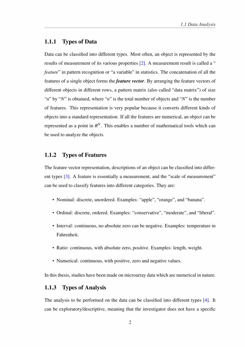
1.1.1 Types of Data
Data can be classified into different types. Most often, an object is represented by the
results of measurement of its various properties [2]. A measurement result is called a “
feature” in pattern recognition or “a variable” in statistics. The concatenation of all the
features of a single object forms the feature vector. By arranging the feature vectors of
different objects in different rows, a pattern matrix (also called “data matrix”) of size
“n” by “N” is obtained, where “n” is the total number of objects and “N” is the number
of features. This representation is very popular because it converts different kinds of
objects into a standard representation. If all the features are numerical, an object can be
represented as a point in RN . This enables a number of mathematical tools which can
be used to analyze the objects.
1.1.2 Types of Features
The feature vector representation, descriptions of an object can be classified into differ-
ent types [3]. A feature is essentially a measurement, and the “scale of measurement”
can be used to classify features into different categories. They are:
• Nominal: discrete, unordered. Examples: “apple”, “orange”, and “banana”.
• Ordinal: discrete, ordered. Examples: “conservative”, “moderate”, and “liberal”.
• Interval: continuous, no absolute zero can be negative. Examples: temperature in
Fahrenheit.
• Ratio: continuous, with absolute zero, positive. Examples: length, weight.
• Numerical: continuous, with positive, zero and negative values.
In this thesis, studies have been made on microarray data which are numerical in nature.
1.1.3 Types of Analysis
The analysis to be performed on the data can be classified into different types [4]. It
can be exploratory/descriptive, meaning that the investigator does not have a specific
2

1.2 Data Mining and Knowledge Discovery
goal and only wants to understand the general characteristics or structure of the data.
It can be confirmatory/inferential, meaning that the investigator wants to confirm the
validity of a hypothesis/model or a set of assumptions using the available data. In pat-
tern recognition, most of the data analysis is concerned with predictive modeling: given
some existing data (“training data”), goal is to predict the behavior of the unseen data
(“testing data”). This is often called “machine learning” or simply “learning.” Depend-
ing on the type of feedback one can get in the learning process, three types of learning
techniques have been suggested [2]. In supervised learning, labels on data points are
available to indicate if the prediction is correct or not. In un-supervised learning, such
label information is missing. In reinforcement learning, only the feedback after a se-
quence of actions that can change the possibly unknown state of the system is given.
In the past few years, a hybrid learning scenario between supervised and un-supervised
learning, known as semi-supervised learning, transductive learning [5], or learning with
unlabeled data [6], has been emerged, where only some of the data points have labels.
This scenario happens frequently in bioinformatics applications, since data collection
and feature extraction can often be automated, whereas the labeling of patterns or ob-
jects has to be done manually, but this job is expensive both in time and cost.
In this thesis, work has been carried out on un-supervised classification i.e., Clustering
to investigate the hidden pattern available in machine learning data as well as bioinfor-
matics data.
1.2 Data Mining and Knowledge Discovery
With the enormous amount of data stored in files, databases, and other repositories, it
is increasingly important, to develop powerful means for analysis and perhaps inter-
pretation of such data and for the extraction of interesting knowledge that could help
in decision-making. Data Mining, also popularly known as Knowledge Discovery in
Databases (KDD), refers to as “the nontrivial process of identifying valid, novel, po-
tentially useful and ultimately understandable pattern in data”. While data mining and
knowledge discovery in databases (KDD) are frequently treated as synonyms, data min-
ing is actually part of the knowledge discovery process. Figure 1.1 shows data mining as
a step in an iterative knowledge discovery process. The task of the knowledge discovery
3

1.2 Data Mining and Knowledge Discovery
and data mining process is to extract knowledge from data such that the resulting knowl-
edge is useful in a given application. The Knowledge Discovery process in Databases
comprises of a few steps leading from raw data collections to some form of retrieving
new knowledge. The iterative process consists of the following steps:
Figure 1.1: Complete Overview of Knowledge discovery from Databases
• Data cleaning: Also known as data cleansing, it is a phase in which noisy data
and irrelevant data are removed from the collection.
• Data integration: At this stage, multiple data sources, often heterogeneous, may
be combined in a common source.
• Data selection: At this step, the data relevant to the analysis is decided on and
retrieved from the data collection.
• Data mining: It is the crucial step in which clever techniques are applied to extract
data patterns potentially useful.
4

1.3 Data Mining Models
• Pattern evaluation: In this step, strictly interesting patterns representing Knowl-
edge is identified based on given measures.
• Knowledge representation: Is the final phase in which the discovered knowledge
is visually represented to the user. This essential step uses visualization tech-
niques to help users understand and interpret the data mining results.
It is common practice to combine some of steps together for specific application. For in-
stance, data cleaning and data integration can be performed together as a pre-processing
phase to generate a data warehouse (1.1). Data selection and data transformation can
also be combined where the consolidation of the data is the result of the selection, or, as
for the case of data warehouses, the selection is done on transformed data. The KDD is
an iterative process. Once the discovered knowledge is presented to the user, the eval-
uation measures can be enhanced, the mining can be further refined, new data can be
selected or further transformed, or new data sources can be integrated, in order to get
different, more appropriate results.
1.3 Data Mining Models
There are several data mining models, some of these are narrated below which are
conceived to be important in the area of “Data Mining” [7], [8].
• Clustering: It segments a large set of data into subsets or clusters. Each cluster is
a collection of data objects that are similar to one another with the same cluster
but dissimilar to object in other clusters [7], [8], [9], [10], [11].
• Classification: Decision trees, also known as classification trees, are a statistical
tool that partitions a set of records into disjunctive classes. The records are given
as tuples with several numerics and categorical attributes with one additional at-
tribute being the class to predict. Decision trees algorithm differs in selection of
variables to split and how they pick the splitting point [7], [8].
• Association Mining: It uncovers interesting correlation patterns among a large set
of data items by showing attribute value conditions that occur together frequently
[7], [8].
5

1.6 Objective
1.4 Application of Data mining
Data mining has become an important area of research since last decade. Important
area where Data mining can be effectively applied are as follows: Health sector (Bi-
ology/Bioinformatics), Image Processing(Image segmentation), Ad-Hoc wireless Net-
work(clustering of nodes), Intrusion detection system, Finance sector etc.
In this thesis focus has been given on clustering techniques and their application to
machine learning and bioinformatics data.
1.5 Motivation
A number of clustering methods have been studied in the literature; they are not satis-
factory in terms of: 1) automation, 2) quality, and 3) efficiency.
• With regard to automation, most clustering algorithms request users to input some
parameters needed to conduct the clustering task. For example, Hard C-means
clustering algorithm ( [7], [8], [9], [10], [11] ) requires the user to input the num-
ber of clusters “C” to be generated. However, in real life applications, it is of-
ten difficult to predict the correct value of ‘C’. Hence, an automated clustering
method is required.
• As for quality, an accurate validation method for evaluating the quality of clus-
tering results is lacking. Consequently, it is difficult to provide the user with
information regarding how good each clustering result is.
• As for efficiency, the existing clustering algorithms(e.g., Hard C-means) may not
perform well when the optimal or near-optimal clustering result is required from
the global point of view.
1.6 Objective
Based on the motivation outlined in the previous section, the main objective of the study
is clustering of gene expression data i.e., to group genes based on similar expressions
over all the conditions. That is, genes with similar corresponding vectors should be
6

1.7 Organization of the Thesis
classified into the same cluster. More specifically, the main objectives of the study is as
follows:
• For cluster formation; C-means algorithm (Hard C-means) [7], [8], [9], [10], [11]
to machine intelligence data as well as to various bioinformatics data (Gene ex-
pression microarray cancer data) and to assess the effectiveness of the algorithm
has been studied.
• To apply soft C-means algorithm (or, Fuzzy C-Means, FCM) ([7], [8], [9], [10],
[11] to same data and to explore how its helps in fuzzy partition of the data (i.e.
how it intends to accommodate one gene to two different clusters at same time
with different degree of membership).
• To propose family of Genetic Algorithm based clustering techniques for multi-
variate data. Four different types of encoding schemes for clustering has been
studied.
• Lastly, a Brute-Force incremental approach for clustering and a Simulated An-
nealing (SA) [12] based method for diversification of the data has been proposed.
• To assess the performance of the proposed model; three Clustering Validation
metrics : Clustering accuracy, HS Ratio [13] and Figure of Merit (FOM [13] )
have been considered.
1.7 Organization of the Thesis
The contents of the thesis is organized as follows:
Chapter 2 discusses the background concepts used in the thesis. First, discussion
has been made on bioinformatics and after that application of clustering to gene expres-
sion microarray data.
Chapter 3 provides a brief review of related work on microarray data and clustering
techniques. Emphasis has been given on research work reported in literature in context
to HCM, SCM and Genetic algorithm based clustering algorithm and their application
to pattern recognition data (machine learning data) and gene expression bioinformatics
data.
7

1.7 Organization of the Thesis
Chapter 4 presents comparative study on conventional Hard C-means clustering
algorithm and Soft C-means clustering. In this chapter, initially discussion has been
made on basic steps involved in Hard C-means and Soft C-means clustering algorithm
and then their application to several machine learning data as well as bioinformatics
data.
Chapter 5 presents Family of Genetic algorithm based clustering algorithm. In this
chapter, first, discussion has been made on basic steps involved in GA based clustering.
Next, discussion has been carried out on four novel methods for representing a chromo-
some and HS Ratio ratio as fitness function for evaluation of fitness of a chromosome.
Later discussion has been made on application of GA based clustering algorithm to
machine learning data and bioinformatics data.
Chapter 6 presents an incremental Brute-Force based clustering method and Sim-
ulated Annealing based method for diversification of the data.
Chapter 7 presents comparative studies on several cluster validation matrices for
assessing the goodness of a clustering algorithm.
Chapter 8 presents the conclusion about work done in this thesis.
8

Chapter 2
Background Concepts
This chapter discusses background concepts, definitions, and notations on bioinformat-
ics and clustering, that are used throughout the thesis.
2.1 Bioinformatics
Bioinformatics ([13], [14], [15], [16]) is the application of information technology to the
field of molecular biology. The term bioinformatics was coined by Paulien Hogeweg in
1978 for the study of informatics processes in biotic systems. The National Center for
Biotechnology Information (NCBI, 2001) defines bioinformatics as “the field of science
in which biology, computer science, and information technology merges into a single
discipline”. There are three important area in bioinformatics: 1.) the development of
new algorithms and statistics with which to assess relationships among members of
large data sets; 2.) the analysis and interpretation of various types of data including nu-
cleotide and amino acid sequences, protein domains, and protein structures; 3.) and the
development and implementation of tools that enable efficient access and management
of different types of information. The explosive growth in the amount of biological data
demands the use of computing systems for the organization, the maintenance and the
analysis of biological data. The aims of bioinformatics are:
1. The organization of data in such a way that allows researchers to access existing
information and to submit new entries as they are produced.
2. The development of tools that help in the analysis of data.
3. The use of these tools to analyze the individual systems in detail, in order to gain
new biological insights.
9

2.1 Bioinformatics
In this thesis, work will be focused on the development of tools that help in the analysis
of data.
2.1.1 Application of Data Mining techniques to Bioinformatics
There are several sub areas in bioinformatics where Data mining can be effectively use
for finding useful information from the biological data [13], [14]. Some of the areas are
described below in brief:
• Data mining in Gene Expression: Gene expression analysis is the use of quan-
titative mRNA-level measurements of gene expression (the process by which a
gene’s coded information is converted into the structural and functional units of a
cell) in order to characterize biological processes and elucidate the mechanisms
of gene transcription [13].
• Data mining in genomics: Genomics is the study of an organism’s genome and
deals with the systematic use of genome information to provide new biological
knowledge ([14]).
• Data Mining in Proteomics: Proteomics is the large-scale study of proteins. Data
mining can be used particularly for prediction of protien’s structures and func-
tions [16].
As far as this thesis is concerned, the main area of focus is application of data mining
techniques to gene expression analysis. In next section, microarray technology has been
described for gene expression data.
2.1.2 Introduction to Microarray Technology
Compared with the traditional approach to genomic research, which is focused on the
local examination and collection of data on single genes, microarray technologies have
now made it possible to monitor the expression levels for tens of thousands of genes
in parallel. The two major types of microarray experiments are the cDNA microarray
and oligonucleotide arrays (abbreviated oligo chip). Despite differences in the details
of their experiment protocols, both types of experiments involve three common basic
procedures ( [13], [14], [15] ) :
10
2.1 Bioinformatics
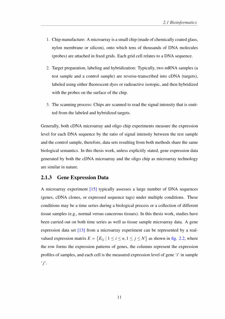
1. Chip manufacture: A microarray is a small chip (made of chemically coated glass,
nylon membrane or silicon), onto which tens of thousands of DNA molecules
(probes) are attached in fixed grids. Each grid cell relates to a DNA sequence.
2. Target preparation, labeling and hybridization: Typically, two mRNA samples (a
test sample and a control sample) are reverse-transcribed into cDNA (targets),
labeled using either fluorescent dyes or radioactive isotopic, and then hybridized
with the probes on the surface of the chip.
3. The scanning process: Chips are scanned to read the signal intensity that is emit-
ted from the labeled and hybridized targets.
Generally, both cDNA microarray and oligo chip experiments measure the expression
level for each DNA sequence by the ratio of signal intensity between the test sample
and the control sample, therefore, data sets resulting from both methods share the same
biological semantics. In this thesis work, unless explicitly stated, gene expression data
generated by both the cDNA microarray and the oligo chip as microarray technology
are similar in nature.
2.1.3 Gene Expression Data
A microarray experiment [15] typically assesses a large number of DNA sequences
(genes, cDNA clones, or expressed sequence tags) under multiple conditions. These
conditions may be a time series during a biological process or a collection of different
tissue samples (e.g., normal versus cancerous tissues). In this thesis work, studies have
been carried out on both time series as well as tissue sample microarray data. A gene
expression data set [13] from a microarray experiment can be represented by a real-
valued expression matrix E ={
Ei j | 1≤ i≤ n,1≤ j ≤ N}
as shown in fig. 2.2, where
the row forms the expression patterns of genes, the columns represent the expression
profiles of samples, and each cell is the measured expression level of gene ‘i’ in sample
‘ j’.
11

2.2 Clustering
Figure 2.1: Microarray Technology: Overview of gene expression analysis using aDNA microarray. (Source: P. O. Brown & D. Botstein, Nat. Genet, Vol. 21, No. 1, pp.33-37, January 1999) .
2.2 Clustering
Clustering [7], [8], [9], [10], [11] is the process of grouping data objects into a set of
disjoint classes, called clusters, so that “objects within the same class have high simi-
larity to each other, while objects in separate classes are more dissimilar”. Clustering
is an example of un-supervised classification. “Classification” refers to a procedure that
assigns data objects to a set of predefined classes. ”Un-supervised” means that clus-
tering does not rely on predefined classes and training examples while classifying the
data objects. Thus, clustering is distinguished from pattern recognition or the areas of
statistics known as discriminate analysis and decision analysis, which seek to find rules
for classifying objects from a given set of pre-classified objects.
12

2.2 Clustering
Figure 2.2: Gene Expression Matrix/Intensity Matrix
Figure 2.3: Complete Overview of Gene Expression Analysis
13

2.2 Clustering
2.2.1 Formal Definition of Clustering
The clustering problem is defined as the problem of classifying ‘n’ objects into ‘C’
clusters without any apriori knowledge [17]. Let the set of ‘n’ points be represented by
the set ‘S’ and the ‘C’ clusters be represented by V1,V2, . . . ,VC. Then
Vi 6= /0 for i = 1,2, . . . ,C,
Vi⋂
V j = /0 for i = 1,2, . . . ,C and i 6= j
and ∪Ci=1Vi = S
2.2.2 Categories of Gene Expression Data Clustering
Typically, microarray experiment contains 103 to 104 genes, and this number is expected
to reach the order of 106. However, the number of samples involved in microarray ex-
periment is generally in the order of 102. One of the characteristics of gene expression
data is that it is meaningful to cluster both genes and samples. Clustering gene expres-
sion data can be categorized into three groups [13].
1. Gene based clustering : In this type of clustering genes are treated as the objects,
while samples as the features. The purpose of gene-based clustering is to group
together co-expressed genes which indicate co-function and co-regulation. Ex-
ample of gene-based clustering which have been used in literature are K-means
[18], SOM [19], CLICK [20], DHC [21], CAST [22], agglomerative hierarchical
[23], model-based clustering [24] etc.
2. Sample based clustering: In this type of clustering samples are the objects and
genes are features. Within a gene expression matrix, there are usually particular
macroscopic phenotype of samples related to some diseases or drug effects, such
as diseased samples, normal samples or drug treated samples. The goal of sample
based clustering is to find the phenotype structures or sub-structures of the sam-
ple. Example of sample-based clustering which have been used in literature are
Xing et. al. [25], Ding. et. al. [26], Hastie et.al. [27], Tang et. al. [28], [29] etc.
3. Subspace Clustering: In this type of clustering, job is to find subsets of objects
such that the objects appear as a cluster in a subspace formed by a subset of the
14

2.2 Clustering
features. In subspace clustering, the subsets of features for various subspace clus-
ters can be different. Two subspace clusters can share some common objects and
features, and some objects may not belong to any subspace cluster. Example of
subspace clustering which have been used in literature are CTWC [30], Biclus-
tering [31], δ − cluster [32], plaid model [33] etc. .
2.2.3 Proximity measurement for Gene Expression Data
Proximity measurement [13] measures the similarity (or, dissimilarity) between two
data objects. Gene expression data objects, no matter genes or samples, can be for-
malized as numerical vectors Ei = {Ei, j | 1≤ j ≤ N}, where Ei, j is the value of the jth
feature for the ith data object and N is the number of features. The proximity between
two objects Ei and E j is measured by a proximity function of corresponding vectors.
There are several proximity measures available in literature like Euclidean Distance,
Pearson correlation coefficient, Jackknife correlation, spearman’s rank-order correla-
tion coefficient etc. A useful review on proximity measurement can be found reference
[7], [8], [9], [10], [11], [13]. Among these all proximity measures, Euclidean Distance
is the simplest one and easy to implement.
2.2.4 Euclidean Distance
Euclidean Distance is one of the most commonly used methods to measure the distance
between two data objects. The distance between objects Ei and E j in N-dimensional
space is defined as:
Euclidean(Ei,E j) =√
∑Nk=1
(Eik−E jk
)2
Euclidean distance does not score well for shifting or scaled patterns (or profiles). To
address this problem, each object vector is standardized with zero mean and variance
one before calculating the distance [7], [8].
In next chapter, discussion has been made on literature work carried out on microarray
data and clustering techniques.
15

Chapter 3
Review of Related Work
This chapter provides overview of research carried out on clustering algorithm and their
application to several microarray data reported in literature. This chapter is broadly
divided into two section. First section deals with research work carried out on several
microarray data and section two deals with research carried out on different clustering
algorithm
3.1 Review work carried out on Microarray data
DNA microarrays are high-throughput methods for analyzing complex nucleic acid
samples. It makes possible to measure rapidly, efficiently and accurately the levels of
expression of all genes present in a biological sample. The application of such methods
in diverse experimental conditions generates lots of data. However, the main problem
with these data occurs while analyzing it. Derivation of meaningful biological infor-
mation from raw microarray data is impeded by the complexity and vastness of the
data [34]. To overcome the problem associated with gene expression microarray data
many statistical methods has been proposed in recent past. Some important has been
explained below:
• Eisen, Spellman, Brown and Botstein (1998) [23]: The paper deals with study on
Hierarchical clustering of gene expression data of budding yeast Saccharomyces
cerevisiae and human gene data. The paper claims that clustering of budding
yeast Saccharomyces cerevisiae gene expression data groups together efficiently
genes of known similar function, and similar tendency were also obtained in hu-
man data. Thus patterns seen in genome-wide expression experiments can be
16

3.1 Review work carried out on Microarray data
interpreted as indications of the status of cellular processes. Also, co-expression
of genes of known function with poorly characterized or novel genes may pro-
vide a simple means of gaining leads to the functions of many genes for which
information is not available currently.
• Tamayo, Slonim, Mesirov, Zhu, Kitaeewan and Dmitrovsky (1999) [19]: This
paper describes the application of self-organizing maps, a type of mathematical
cluster analysis that is particularly well suited for recognizing and classifying fea-
tures in complex, multidimensional data. The method has been implemented in
a publicly available computer package, GENECLUSTER, that performs the an-
alytical calculations and provides easy data visualization. To illustrate the value
of such analysis, the approach is applied to hematopoietic differentiation in four
well studied models (HL-60, U937, Jurkat, and NB4 cells). Expression patterns
of some 6,000 human genes were assayed, and an online database was created.
GENECLUSTER was used to organize the genes into biologically relevant clus-
ters that suggest novel hypotheses about hematopoietic differentiation. For exam-
ple, highlighting certain genes and pathways involved in ‘differentiation therapy’
used in the treatment of acute promyelocytic leukemia.
• Iyer, Eisen, Ross, Schuler, Moore, Lee, Trent, Hudson, Boguski, Lashkari, Bost-
tein, and Brown (1999) [35]: The paper deals with temporal program of gene
expression during a model physiological response of human cells, the response
of fibroblasts to serum, was explored with a complementary DNA microarray
representing about 8600 different human genes. Genes could be clustered into
groups on the basis of their temporal patterns of expression in this program. Many
features of the transcriptional program appeared to be related to the physiology
of wound repair, suggesting that fibroblasts play a larger and richer role in this
complex multicellular response than had previously been appreciated.
• Chu, Eisen, Mulholland, Botstein, Brown and Herskowitz (1998) [36]: The pa-
per deals with developmental program of sporulation of budding yeast. Diploid
cells of budding yeast produce haploid cells through the developmental program
17

3.1 Review work carried out on Microarray data
of sporulation, which consists of meiosis and spore morphogenesis. DNA mi-
croarrays containing nearly every yeast gene were used to assay changes in gene
expression during sporulation. At least seven distinct temporal patterns of induc-
tion were observed. The transcription factor Ndt80 appeared to be important for
induction of a large group of genes at the end of meiotic prophase. Consensus
sequences known or proposed to be responsible for temporal regulation could be
identified solely from analysis of sequences of coordinately expressed genes. The
temporal expression pattern provided clues to potential functions of hundreds of
previously uncharacterized genes, some of which have vertebrate homologs that
may function during gametogenesis.
• Spellman, Sherlock, Iyer, Zhang, Anders, Eisen, Brown and Bostein (1998) [37] :
This paper creates a comprehensive catalog of yeast genes whose transcript levels
vary periodically within the cell cycle. To this end, DNA microarrays have been
used and samples from yeast cultures synchronized by three independent meth-
ods: alpha factor arrest, elutriation, and arrest of a cdc15 temperature-sensitive
mutant. Using periodicity and correlation algorithms, 800 genes were identified
that meet an objective minimum criterion for cell cycle regulation. In separate ex-
periments, designed to examine the effects of inducing either the G1 cyclin Cln3p
or the B-type cyclin Clb2p, It was found that the mRNA levels of more than half
of these 800 genes respond to one or both of these cyclins. Furthermore, anal-
ysis was done on set of cell cycle-regulated genes for known and new promoter
elements and show that several known elements (or variations thereof) contain
information predictive of cell cycle regulation.
• Roth, Estep, and Church (1998) [38] :In this paper Whole-genome mRNA quan-
titation was used to identify the genes that are most responsive to environmental
or genotypic change. By searching for mutually similar DNA elements among
the upstream non-coding DNA sequences of these genes, identification of can-
didate regulatory motifs and corresponding candidate sets of co-regulated genes
can be made. This strategy was tested by applying it to three extensively studied
regulatory systems in the yeast Saccharomyces cerevisiae: galactose response,
18

3.1 Review work carried out on Microarray data
heat shock, and mating type. Galactose-response data yielded the known binding
site of Gal4, and six of nine genes known to be induced by galactose. Heat shock
data yielded the cell-cycle activation motif, which is known to mediate cell-cycle
dependent activation, and a set of genes coding for all four nucleosomal proteins.
Mating type alpha and a data yielded all of the four relevant DNA motifs and
most of the known a and alpha-specific genes.
• Cho R. J., Campbell M. J., Winzeler E. A., Steinmetz L., Conway A., Wodicka
L., Wolfsberg T. G., Gabrielian A. E., Landsman D., Lockhart D. J., Davis R.W.
(1998) [39]: The paper deals with the genome-wide characterization of mRNA
transcript levels during the cell cycle of the budding yeast S. cerevisiae. Cell
cycle-dependent periodicity was found for 416 of the 6220 monitored transcripts.
More than 25 % of the 416 genes were found directly adjacent to other genes
in the genome that displayed induction in the same cell cycle phase, suggesting
a mechanism for local chromosomal organization in global mRNA regulation.
More than 60 % of the characterized genes that displayed mRNA fluctuation have
already been implicated in cell cycle period-specific biological roles. Because
more than 20 % of human proteins display significant homology to yeast pro-
teins, these results also link a range of human genes to cell cycle period-specific
biological functions.
• Bhattacharjee A., Richards WG, Staunton J, Li C, Monti S, Vasa P, Ladd C, Be-
heshti J,Bueno R, Gillette M, Loda M, Weber G, Mark EJ, Lander ES, Wong W,
Johnson BE, Golub TR, Sugarbaker DJ, Meyerson M.(2001) [40]: In this paper
a molecular taxonomy of lung carcinoma has been generated. Using oligonu-
cleotide microarrays, analysis was made on mRNA expression levels correspond-
ing to 12,600 transcript sequences in 186 lung tumor samples, including 139 ade-
nocarcinomas resected from the lung. Hierarchical and probabilistic clustering
of expression data defined distinct subclasses of lung adenocarcinoma. Among
these were tumors with high relative expression of neuroendocrine genes and of
type II pneumocyte genes, respectively. Retrospective analysis revealed a less fa-
vorable outcome for the adenocarcinomas with neuroendocrine gene expression.
19

3.1 Review work carried out on Microarray data
The diagnostic potential of expression profiling is emphasized by its ability to
discriminate primary lung adenocarcinomas from metastases of extra-pulmonary
origin. The results shown in paper suggest that integration of expression profile
data with clinical parameters could aid in diagnosis of lung cancer patients.
• Golub T. R., Slonim D. K. , Tamayo P., Huard C., Gaasenbeek M., Mesirov J.
P., Coller H., Loh M. L. , Downing J. R., Caligiuri M. A., Bloomfield C. D.,
Lander E. S. (1999) [41]: In this paper, a generic approach to cancer classifica-
tion based on gene expression monitoring by DNA microarrays was described
and applied to human acute leukemias as a test case. A class discovery proce-
dure automatically discovered the distinction between acute myeloid leukemia
(AML) and acute lymphoblastic leukemia (ALL) without previous knowledge of
these classes. An automatically derived class predictor was able to determine the
class of new leukemia cases. The results demonstrate the feasibility of cancer
classification based solely on gene expression monitoring and suggest a general
strategy for discovering and predicting cancer classes for other types of cancer,
independent of previous biological knowledge.
• Laura J., Van ’t veer [42]: The paper deals with Breast cancer microarray data.
Breast cancer patients with the same stage of disease can have markedly different
treatment responses and overall outcome. The strongest predictors for metastases
(for example, lymph node status and histological grade) fail to classify accurately
breast tumours according to their clinical behaviour. Chemotherapy or hormonal
therapy reduces the risk of distant metastases by approximately one-third; how-
ever, 70-80 % of patients receiving this treatment would have survived without
it. None of the signatures of breast cancer gene expression reported to date al-
low for patient-tailored therapy strategies. In the paper, DNA microarray analysis
on primary breast tumours of 117 young patients has been carried out, and ap-
plied supervised classification to identify a gene expression signature strongly
predictive of a short interval to distant metastases (‘poor prognosis’ signature) in
patients without tumour cells in local lymph nodes at diagnosis (lymph node neg-
ative). In addition, a signature that identifies tumours of BRCA1 carriers has been
20

3.1 Review work carried out on Microarray data
established. The poor prognosis signature consists of genes regulating cell cycle,
invasion, metastasis and angiogenesis. This gene expression profile outperforms
all currently used clinical parameters in predicting disease outcome.
• West M., Blanchette C., Dressman H., Huang E., Ishida S., Spang R., Zuzan H.,
Olson J. A. Jr., Marks J. R., Nevins J. R. (2001) [43]: In this paper, Bayesian
regression models has been developed that provide predictive capability based
on gene expression data derived from DNA microarray analysis of a series of
primary breast cancer samples. These patterns have the capacity to discriminate
breast tumors on the basis of estrogen receptor status and also on the categorized
lymph node status. Importantly, in the paper assessment was done on the utility
and validity of such models in predicting the status of tumors in cross-validation
determinations. The practical value of such approaches relies on the ability not
only to assess relative probabilities of clinical outcomes for future samples but
also to provide an honest assessment of the uncertainties associated with such
predictive classifications on the basis of the selection of gene subsets for each
validation analysis. This latter point is of critical importance in the ability to
apply these methodologies to clinical assessment of tumor phenotype.
• Shipp M. A., Ross K. N., Tamayo P., Weng A.P., Kutok J. L., Aguiar R. C.,
Gaasenbeek M., Angelo M., Reich M., Pinkus G. S., Ray T. S., Koval M. A.,
Last K. W., Norton A., Lister T. A., Mesirov J.,Neuberg D. S., Lander E. S.,
Aster J. C., Golub T. R. (2002) [44]: Diffuse large B-cell lymphoma (DLBCL),
the most common lymphoid malignancy in adults, is curable in less than 50 %
of patients. Prognostic models based on pre-treatment characteristics, such as the
International Prognostic Index (IPI), are currently used to predict outcome in DL-
BCL. However, clinical outcome models identify neither the molecular basis of
clinical heterogeneity, nor specific therapeutic targets. In this paper analysis has
been done on the expression of 6,817 genes in diagnostic tumor specimens from
DLBCL patients who received cyclophosphamide, adriamycin, vincristine and
prednisone (CHOP)-based chemotherapy, and applied a supervised learning pre-
diction method to identify cured versus fatal or refractory disease. The algorithm
21

3.2 Review on Clustering algorithm
classified two categories of patients with very different five-year overall survival
rates (70% versus 12%). The model also effectively delineated patients within
specific IPI risk categories who were likely to be cured or to die of their disease.
Genes implicated in DLBCL outcome included some that regulate responses to
B-cell-receptor signaling, critical serine/threonine phosphorylation pathways and
apoptosis. Result shown in paper indicates that supervised learning classifica-
tion techniques can predict outcome in DLBCL and identify rational targets for
intervention.
3.2 Review on Clustering algorithm
Lots of work has been done in clustering in recent past. A useful review on clustering
can be found out from the following referenced paper [7], [8], [9], [10], [13], [34], [45],
[46]. In this section, discussion has been made on various work done in literature on
HCM, SCM and GA based clustering.
3.2.1 Review on Hard C-means Clustering Algorithm
The Hard C-means clustering (HCM) algorithm is one of the best-known squared error-
based clustering algorithm [7], [8], [9], [10]. It is very simple and can be easily im-
plemented in solving many practical problems. It can work very well for compact and
hyper-spherical clusters. The time complexity of Hard C-means is ‘O(n×C×N)’ and
space complexity is ‘O(n +C)’, where ‘n’ is number of data points, ‘N’ is number of
feature and ‘C’ is number of cluster in consideration. Since ‘C’ and ‘N’ are usually
much less than ‘n’, Hard C-means can be used to cluster large data sets in least time.
The HCM algorithm has been extensively applied in several areas [7], [8], [9], [10].
HCM algorithm has been extensively studied in the past for its applicability to pattern
recognition and machine learning data. Application of HCM to Iris data has been re-
ported in paper [47], [48], [49], [46]. The number of wrongly clustered instances in
case of Iris may vary from 14 to 17 [47]. HCM has also been used in recent past in case
of WBCD [46]. Application of HCM clustering algorithm to microarray gene expres-
sion analysis has been also reported in literature [18], [50]. Herwig et. al. developed
a variant of HCM algorithm and applied to cluster a set of 2029 human cDNA clones
22

3.2 Review on Clustering algorithm
and adopted mutual information as the similarity measure [50]. Tavazoie et al. par-
titioned 3 000 genes into 30 clusters with the HCM algorithm [18]. For each cluster,
600 base pairs upstream sequences of the genes were searched for potential motifs. 18
motifs were found from 12 clusters in their experiments and 7 of them can be veri-
fied according to previous empirical results in the literature. A more comprehensive
investigation can be found in [18]. Application of HCM algorithm to DNA or protein
sequences clustering has been reported in paper [51]. In paper [51], protein or DNA se-
quences were transformed into a new feature space based on the detected sub-patterns
and subsequently clustered with the HCM algorithm [51].
The drawbacks of HCM are also well studied in literature. Some of the major dis-
advantages are as follows:
1. There is no efficient and universal method for identifying the initial partitions in
Hard C-means clustering algorithm. The convergence centroids vary with dif-
ferent initial points and that may results in suboptimal solution. This particular
limitation of Hard C-means clustering algorithm has been extensively studied in
literature such as [11], [52], [53], [54], [55], [56], [57], [58], [59], [60], [61], [62],
[63], [64]. This problem is still an open issue of research.
2. The iteratively optimal procedure of Hard C-means cannot guarantee convergence
to a global optimum. This particular problem was addressed in following pa-
per: [65], [66], [67], [64], [12] The stochastic optimal techniques, like simulated
annealing (SA), tabu search and genetic algorithms can be clubbed with Hard
C-means to find the global optimum [9], [10].
3. Hard C-means algorithm is also sensitive to outliers and noise. Even if an object
is quite far away from the cluster centroid, it is still forced into a cluster and, thus,
distorts the cluster shapes [55], [11], [68].
4. The Hard C-means algorithm is limited to numerical variables [55], [68], [69],
[70].
5. Determining the optimal number of clusters in a set of data is prerequisite to Hard
23

3.2 Review on Clustering algorithm
C-means clustering algorithm [55], [71], [72], [73], [74], [75], [76], [77], [78],
[79], [80], [81], [82]
3.2.2 Review on Soft C-means based Clustering Algorithm
Soft C-means is a generalization of Hard C-means clustering algorithm. SCM is a
method of clustering which allows a data point to belong to two or more clusters at a
time. This method was developed by Dunn in 1973 [83] and improved by Bezdek in
1981 [84]. It is based on minimization of an objective function called, Mean square
Error (MSE). SCM was frequently used in pattern recognition.
A detailed work on SCM can be found out from the paper [85], [86], [87], [88], [89],
[90], [91], [91], [92], [93].
Several work has been also done on gene expression analysis using SCM [94],[95],
[96], [97], [98], [99], [100], [101].
3.2.3 Review on Genetic Algorithm based Clustering
Clustering can be formally formulated as a NP-hard grouping problem in optimization
perspective [102]. This research finding has stimulated the search for efficient approxi-
mation algorithms, including not only the use of ad-hoc heuristics for particular classes
or instances of problems, but also the use of general-purpose metaheuristics [103]. Par-
ticularly, evolutionary algorithms are metaheuristics widely believed to be effective on
NP-hard problems, being able to provide near-optimal solutions to such problems in
reasonable time. Under this assumption, a large number of evolutionary algorithms
for solving clustering problems have been proposed in the literature [34]. These al-
gorithms are based on the optimization of some objective function (i.e., the so-called
f itness f unction) that guides the evolutionary search. In evolutionary algorithm, Ge-
netic algorithm (GA) becomes natural choice for cluster formation algorithm due to
its wide applicability in wide range of areas. Problem representation is one of the key
decision to be made when applying a GA to a problem. Problem representation in a
GA individual determines the shape of the solution space that a GA must search. As a
result, different encodings of the same problem are essentially different problems for a
GA [104]. The application of GAs for solving problems of pattern recognition appears
24

3.3 Conclusion
to be appropriate and natural. Research articles in this area have reported in literature
[105], [106], [107], [108], [109], [110], [111], [112], [113], [114]. An application of
GAs has been also reported in the area of (supervised) pattern classification for design-
ing a GA-classifier [107], [115]. GA based Clustering algorithm for machine learning
data was reported in the literature [116], [17], [117], [118].
The paper [17] is specific to pattern recognition data. There are no extensive work
reported in literature for bioinformatics data specially for microarray cancer data using
GA.
3.3 Conclusion
Due to advancement of DNA microarray technology, researchers now have the ability to
collect expression data on every gene in a cell simultaneously. The vast datasets created
with this technology are providing valuable information that can be used to accurately
diagnose, prevent, or cure a wide range of genetic and infectious diseases. Thus, an area
of active research is the development of tools to accurately collect, analyze, and inter-
pret massive quantities of data on gene expression levels in the cell. There are several
examples in the literature where computational tools have been applied to analyze gene
expression data. The summary of these microarray data and tools are given in Table 3.1
( [45]).
25

3.3 Conclusion
Table 3.1: Summary of work done in Literature on Microarray using classifica-tion(supervised/unsupervised) Source: [45]Data Set Description Method
Cho’s Data [39] 6,200 ORFs in S cerevisiae with 15 time points K-Means [18], SOM[19], CLICK [20], DHC[21], Biclustering [31],δ -Cluster [32]
Iyer’s Data [35] 9.800 cDNAs with 12 time points agglomerative hierarchi-cal [23], [20], DHC [21]
Wen’s Data[119]
112 rat genes during 9 time points CAST [22]
Combinedyeast Data [36],[120], [37]
6,178 ORFs in S cerevisiae with 4 time courses agglomerative hierarchi-cal [23], model-based[121], Plaidmodel [33]
Colon cancerdata [122]
6,500 human genes in 40 tumor and 22normalcolon tissue samples
divisive hierarchical[122], model-based [24]
C.elegans data 1,246 genes in 146 experiments CAST [22]
humanhematopoi-etic data
(1)6,000 genes in HL-60 cell lines with 4 timepoints (2)6,000 genes in 4 cell lines (HL-60, U937and jurkat with 4 time points and NB4 with 5 timepoints)
SOM [19]
Leukemia Data[41]
7,129 genes, 72 Samples (25 AML, 47 All) Some supervised meth-ods Xing et. al. [25] andDing et. al. [26], CTWC[30]
LymphomaData [123]
4,096 genes, 96 Samples(46 DLBCL, 50 Normal) Some supervised meth-ods Ding et. al. [26],Hastie et al. [27], Bi-clustering [31]
Colon cancerData [122]
2,000 genes, 62 Samples Some supervised meth-ods, CTWC [30]
HereditaryBreast cancerData
3,226 genes, 22 Samples(7BRCA1,8BRCA2,7Sporadic)
Some supervised meth-ods
Multiple Sclero-sis data [124]
4,132 genes, 44 Samples (15 MS, 14 IFN, 15 Con-trol)
Tang et al. [28], [29]
26

Chapter 4
Comparative Study On Hard C-meansand Soft C-means ClusteringAlgorithm
Clustering techniques can be broadly divided into two types: Hard and Soft clustering
algorithm. A Hard clustering algorithm allocates each pattern (or, data point) to a single
cluster during its operation and in its output whereas a soft clustering method assigns
degrees of membership in several clusters to each input pattern. A soft clustering can be
converted to a hard clustering by assigning each pattern to the cluster with the largest
measure of membership [10]. In this chapter, study has been carried out on Hard C-
means (HCM) clustering and Soft C-means (SCM) clustering algorithm.
This chapter is broadly divided into four section:
• Experimental Setup to simulate Hard C-means and Soft C-means clustering algo-
rithm
• Hard C-means Clustering Algorithm ([7], [8], [9], [10])
• Soft C-means Clustering Algorithm ([83], [84])
• Comparative studies on HCM Clustering Algorithm and SCM Clustering Algo-
rithm
4.1 Experimental Setup
In this section, details about various datasets used for simulating cluster formation algo-
rithm to solve “gene expression analysis problem” has been given. Two pattern recog-
nition data and thirteen bioinformatics data were taken for simulation study. Study has
27

4.1 Experimental Setup
been made on almost all benchmark bioinformatics data reported in last decade in lit-
erature. In order to identify common subtypes (cluster within clusters) in independent
disease data: four different types of breast data (Golub et. al) and four DLBCL (Dif-
fused Large B-cell Lymphoma) data are considered for our study on both gene/sample
data as well as time series microarray data. The short description of the datasets along
with their size, no. of clusters and source of the data has been given in Table 4.1. These
datasets are having both overlapping and non-overlapping class boundaries, where the
number of features/genes ranges from 4 to 7129 and number of sample ranges from 32
to 683. The number of cluster ranges from 2 to 11. Details about these data can be
found out from respective referenced paper. All the data have been pre-processed in
such a way that all the data point which belongs to class 1 in original datasets is kept
together, then all the data points which belong to class 2 is kept together and so on. The
reference vector (class information) of resultant data are given in appendix B. The snap
shots of a dataset (e.g., iris data) is given in appendix A. The details of all the fifteen
datasets are given in subsection below.
4.1.1 Datasets
This section deals with dataset used to simulate proposed clustering algorithm. ‘Two’
machine learning and ‘thirteen’ bioinformatics data have been taken to simulate clus-
tering algorithm to solve “gene expression analysis problem”. Brief introduction about
the data is given below:
Machine Learning Data (Pattern Recognition Data)
1. Iris Data
The Iris data set [125] is a well known and well used benchmark data set used
in the machine learning community. The dataset consists of three varieties of
Iris; Setosa, Virginica and Versicolor. There are ‘150’ instances of plants that
make up the three classes. The data consists of four independent variables. These
variables are measurement of the flowers of the plants such as sepal and petal
lengths. Since the data are labeled, it has been extensively used for classifica-
tion purpose in previous work. For clustering, the labeled information avail-
able to Iris data was not used while forming clusters. The size of the data is
28

4.1 Experimental Setup
[150x4].The characteristic of this data is it’s having some overlap between classes
2 and 3. The minimum and maximum feature values in Iris are 0.1 and 7.7. Since
the number of classes in this data is three therefore the value of the ‘C’ cho-
sen to be 3. The original data can be obtained from UCI repository websites:
http://archive.ics.uci.edu/ml/datasets/Iris). The snap shots of iris data is given in
appendix A.
2. Wisconsin Breast Cancer Data (WBCD)
Breast cancer is one of the most common cancers in women and a frequent
cause of death in the 35-55 year age group. The presence of a breast mass is
an alert sign, but it does not always indicate a malignant cancer. Non-invasive
diagnostic test (e.g., Fine needle aspiration of breast masses), that obtains in-
formation needed to evaluate malignancy. The Wisconsin Breast Cancer dataset
was initially created to conduct experiments that were to prove the usefulness
of automation of fine needle aspiration cytological diagnosis. It contains 699
instances of cytological analysis of fine needle aspiration from breast tumors.
Each case comprises 11 attributes: a case ID, cytology data (normalized, with
values in the range ‘1-10’) and a benign/malignant attribute. The number of be-
nign instances is ‘458’ (65.52%) and the number of malignant instances is ‘241’
(34.48%). Sixteen instances of cases (‘14’ benign, ‘2’ malignant) with miss-
ing values has been removed from the dataset for simulation study. The origi-
nal WBCD data [126], [127] can be downloaded from UCI repository websites
(http://archive.ics.uci.edu).
Gene Expression Microarray Data (Bioinformatics Data)
The gene expression datasets and a very short description of their characteristics
are given in Table 4.1. Further biological details about these data sets can be
found in the referenced papers. Most data were processed on the Human Genome
U95 Affymetrix “c” microarrays. The Leukemia dataset is from the previous-
generation Human Genome HU6800 Affymetrix ‘c’ microarray.
3. Iyer data (serum data)
This data set is previously described and has been used in paper [35]. It can
29

4.1 Experimental Setup
be downloaded from: http: //www.sciencemag.org/feature/data/984559.shl. It
corresponds to the selection of ‘517’ genes whose expression varies in response
to serum concentration in human fibroblasts and is classified into ‘11’ groups.
4. Cho data (Yeast data)
In this data set [39], [18] the expression pro-files of 6200 yeast genes were mea-
sured every 10 minute during two cell cycles in 17 hybridization experiments.
Tavazoie et. al. [18] used the Yeast data of 2945 genes. He selected the data
after excluding time points 90 and 100 minute from Yeast data. In this thesis,
386 genes from Cho data has been considered for analysis of experimental work
[128]. Total no. of classes for this data is 5.
5. Leukemia (Golub experiment)
The Leukemia dataset belongs to two types of Leukemia cancers [41], [129]:
Acute Myeloid Leukemia (AML) and Acute Lymphoblastic Leukemia (ALL). It
consists of ‘72’ samples of ‘7129’ gene expressions each. The data has ‘47’ sam-
ples belong to ALL cancer class and ‘25’ samples belong to AML cancer class.
Breast data
The microarray breast data used in this paper can be downloaded from
http://www.broad.mit.edu/cgi-bin/cancer/datasets.cgi.
6. Breast data A [42]
This data is of dimension [98x1213] and total number of classes for this data is
three.
7. Breast data B [43]
This data is of dimension [49x1024] and total number of classes for this data is
three.
8. Breast Multi data A [130]
This data is of dimension [103x5565] and total number of classes for this data is
four.
30

4.1 Experimental Setup
9. Breast Multi data B [131]
This data is of dimension [32x5565] and total number of classes for this data is
four.
Lymphoma data (Alizadeh et al. Experiment)
This datsets describes systematic characterization of gene expression patterns in
the most prevalent adult Lymphoid malignancies: Diffused Large B Cell Lym-
phoma (DLBCL) [123]. In addition, non-lymphoma (normal) samples are also
involved because of the suspected correlation between them and the three malig-
nances. Within DLBCL class, there are two molecularly distinct forms of DL-
BCL which have gene expression patterns indicative of different stages of B-cell
differentiation (1. Germinal centre B cells (‘GC B-like DLBCL’); 2.‘Activated B-
like DLBCL’). These two subtypes of DLBCL have clinically distinct meanings:
patients with germinal centre B-like DLBCL have a significantly better overall
survival than those with activated B-like DLBCL. The molecular classification of
tumors on the basis of gene expression can thus identify previously undetected
and clinically significant subtypes of cancer. Four subtypes of DLBCL (DLBCL
A, DLBCL B, DLBCL C, DLBCL D) has been used to analyze experimental
work. All these Data can be downloaded from http://www.broad.mit.edu/cgi-
bin/cancer/datasets.cgi.
10. DLBCL A [132]
The size of DLBCL A data is [141 X 661] and number of cluster is three.
11. DLBCL B [133]
The size of DLBCL B data is [180 X 661] and number of cluster is three.
12. DLBCL C [44]
The size of DLBCL C data is [58 X 1772] and number of cluster is four.
13. DLBCL D [132]
The size of DLBCL D data is [129 X 3795] and number of cluster is four.
31

4.2 Hard C-means (HCM) Clustering Algorithm
14. Lung Cancer [40]
This microarray datasets [40] is of dimension [197x581]. It includes 4 known
classes: 139 adenocarcinomas (AD), 21 squamous cell carcinomas (SQ), 20 car-
cinoids (COID), and 17 normal lung (NL). The AD class is highly heterogeneous,
and substructure is known to exist, although not well understood. The source of
data is: http://www.broad.mit.edu/cgi-bin/cancer/datasets.cgi .
15. St. Jude Leukemia data [134]
This datasets [134] is of diagnostic bone marrow samples from pediatric acute
Leukemia patients corresponding to 6 prognostically important Leukemia sub-
types: 43 T-lineage ALL; 27 E2A-PBX1, 15 BCR-ABL, 79 TEL-AML1, and 20
MLL rearrangements; and 64 ”hyperdiploid ≥ 50” chromosomes. The source of
data is: http://www.broad.mit.edu/cgi-bin/cancer/datasets.cgi .
Table 4.1: Datasets with known ground truth value (i.e. class label information areknown)
Sl.No.
Datasets Source Dimension Number ofcluster
1 Iris [125] [150x4] 32 WBCD [126], [127] [683x9] 23 Iyer data/Serum data [35] [517x12] 114 Cho data (yeast data) [39] [18] [386x16] 55 Leukemia (Golub xperiment) [41], [129] [72x7129] 26 Breast data A [42] [98x1213] 37 Breast data B [43] [49x1024] 48 Breast Multi data A [130] [103x5565] 49 Breast Multi data B [131] [32x5565] 410 DLBCL A [132] [141x661] 311 DLBCL B [133] [180x661] 312 DLBCL C [44] [58x1772] 413 DLBCL D [132] [129x3795] 414 Lung Cancer [40] [197x581] 415 St. Jude Leukemia data [134] [248x985] 6
In next section (section 4.2 ), First discussion has been made on basic steps involved
in HCM Clustering Algorithm and then how it can be used for Gene/Sample clustering.
4.2 Hard C-means (HCM) Clustering Algorithm
This section describes HCM clustering algorithm and their application to machine in-
telligence data as well as to bioinformatics data. First, basic steps involved in HCM
32

4.2 Hard C-means (HCM) Clustering Algorithm
Table 4.2: Hard C-means Clustering AlgorithmNotations:X: Datasets;Xi: ith Data point of X;x: any data point in X;n : Total Number of data point in X;N : Dimension of each data;Vj= jth Cluster;C : Number of Clusterv j = jth Cluster Center;v∗j = jth Cluster Center after updation;i, j, and p : index variableInput:Given datasets X; total number of data is ‘n’; each data is of dimension ‘N’. Therefore datasetX = {X1,X2, . . . ,Xn} .Total Number of Cluster is: C.Output:V1, V2,...VC.Objective Function:J = ∑C
j=1 ∑xi∈V j ‖ xi− v j ‖2 j ∈ 1,2, . . .,C and i = {1,2, . . .,n}.Hard C-means Clustering Algorithm:Step 1: Chose “C” initial cluster centers(i.e. Prototype vector) v1,v2, . . .vC either randomly or usingany intelligent techniques from the given ’n’ data points X1,X2, . . . ,Xn.Step 2: Now compute ‖ Xi− v j ‖ and ‖ Xi− vp ‖ f or p ∈ 1,2, . . .C, but p 6= j.if ‖ Xi− v j ‖< ‖ Xi− vp ‖ f or p ∈ 1,2, . . .C, but p 6= j where Xi, i = 1,2, ,n;Then put data X in cluster Vj.If any ties occurred, then resolved it arbitrarily.Step 3: Compute new cluster centers {v∗1,v
∗2, ...,v
∗c} as follows:
v∗j = 1|V j | ∑xi∈V j xi , j = 1,2, . . .,C, Where |Vj | = is the number of elements belonging to
cluster Vj.Step 4: If v∗j = v j ; j = 1,2, . . . ,C ; then terminate. Otherwise repeat from step 2.Step 5: If the process does not terminate at Step 4 normally, then it is executed for a maximum“fixed number of iterations”.
clustering algorithm has been explained in details and then experiment are carried out
to assess the performance of HCM clustering algorithm.
The HCM clustering algorithm ([7], [8], [9], [10] ), one of the most widely used
clustering techniques, attempts to solve the clustering problem by optimizing a objec-
tive function J, which is Mean Square Error (MSE) of formed cluster. The objective
function J is given as follows: Minimize(J) = ∑Cj=1 ∑xi∈V j ‖ xi− v j ‖2 j ∈ 1,2, . . .,C
and i = {1,2, . . .,n}.
The basic steps involved in HCM clustering algorithm are briefly described in Table
4.2.
33

4.2 Hard C-means (HCM) Clustering Algorithm
4.2.1 Result And Discussions
To validate the feasibility and performance of the HCM clustering algorithm, HCM
clustering has been implemented in MATLAB 7.0 (Intel C2D processor, 2.0 GHz,
2 GB RAM) and applied it to Machine learning data as well as to bioinformatics
data. Since the datasets used for simulation studies possess class label information,
clustering accuracy has been used as cluster validation metric to judge quality of the
cluster formation algorithm. Clustering Accuracy is defined as follows:
Clustering Accuracy = (Number o f Correct Count
Total number o f instances genes/samples) ∗ 100
. Complete result of Hard C-means clustering for machine learning and bioinformatics
data has been given in appendix C and appendix E. Appendix C contains the details
of data distribution after simulation of HCM clustering algorithm and Appendix E con-
tains the details of data point wrongly clustered in each cluster after simulation of HCM
clustering algorithm. Here in this section, result obtained for HCM clustering algorithm
has been discussed in brief.
Table 4.3 represents summary of result using HCM clustering algorithm for fifteen
datasets. It also consists of some important relevant characteristics, such as number
of classes, number of features/genes and the number of item samples. Out of fifteen
datasets maximum accuracy was reported for WBCD data while least accuracy data
was reported for DLBCL D (Table 4.3). As far as gene expression data is concerned
maximum accuracy was achieved in case of St. Jude Leukemia data (Table 4.3).
Table 4.4 represents the result of Iris data. Overall accuracy has been achieved upto
88.67%. The total count error in this case is 17. It may be noted that 100% accuracy
has been obtained for cluster 1. Similar sort of result for Iris data has been also reported
in literature [47], [48], [49].
Table 4.6 represents the result of Serum data (Iyer data). Accuracy upto 51.84% has
been obtained in this case.
Table 4.5 represents the result of WBCD data. 95.75% accuracy has been achieved in
this case.
Table 4.7 represents the result of Yeast data (Cho data). Overall Accuracy upto 60.88
% has been obtained for this data. It may be noted that cluster 4 is having lowest ac-
34

4.2 Hard C-means (HCM) Clustering Algorithm
curacy of 12%. The reason for this is that data belonging to this cluster are very much
overlapping in nature with other clusters.
Table 4.8 represents the result of Leukemia data. Over all accuracy upto 59.72% has
been obtained. The Golub et. al.’s microarray data [41], [129] is very challenging be-
cause the appearance of the two types of acute Lseukemia features are highly similar
in nature. This was the reason, accuracy was low in this case. One probable solution
of this problem could be the use of dimensionality reduction techniques to reduce the
number of features and then use HCM clustering algorithm.
Table 4.9 to Table 4.12 represents the result of subtypes of Breast data. Maximum ac-
curacy was obtained for Breast Multi data A (79.61%) whereas the least accuracy for
Breast data B was (53.06%). The reason of the less accuracy could be probably Breast
data B is more overlapping in nature and is having nonlinear structure.
Table 4.13 to Table 4.16 represents the result of subtypes of DLBCL data (Diffused
Large B-cell Lymphoma). DLBCL D is of highly overlapping in nature and that’s why
least accuracy of 42.64% has been obtained in this case. The data of DLBCL B is of
highly distinctively separated in nature compared to other data such as DLBCL (A, C,
D) and that is the reason higher accuracy was obtained in case of DLBCL B.
Table 4.17 represents the result of Lung Cancer. Accuracy upto 72.08% has been ob-
tained. In this, cluster 2 and cluster 4 are highly separable in nature compared to cluster
1 and cluster 3. 95% accuracy was obtained for cluster 2 and cluster 4, whereas least
accuracy was obtained for cluster 3 i.e., 47%.
Table 4.18 represents the result of St. Jude Leukemia data. For this data accuracy upto
85.08% was obtained. The data in this case is of highly separable in nature. 100%
accuracy has been obtained for cluster 2 and least one was obtained for cluster 5.
35

4.2 Hard C-means (HCM) Clustering Algorithm
Table 4.3: Summary of Results for Hard C-means using all fifteen datasetsSl.No.
Datasets Dimension # ofcluster
Hard C-means
# Error Error (%) # correct Accuracy(%)
1 Iris [150x4] 3 17 11.33 133 88.672 WBCD [683x9] 2 29 4.25 654 95.753 Iyer data/Serum
data[517x12] 11 249 48.1624 268 51.84
4 Cho data (yeastdata)
[386x16] 5 151 39.1191 235 60.88
5 Leukemia(GolubExperiment)
[72x7129] 2 29 40.28 43 59.72
6 Breast data A [98x1213] 3 27 27.55 71 72.447 Breast data B [49x1024] 4 23 46.93 26 53.06128 Breast Multi data
A[103x5565] 4 21 20.39 82 79.61
9 Breast Multi dataB
[32x5565] 4 15 48.88 17 53.125
10 DLBCL A [141x661] 3 66 46.8085 75 53.19111 DLBCL B [180x661] 3 40 22.22 140 77.7812 DLBCL C [58x1772] 4 28 48.28 30 51.724113 DLBCL D [129x3795] 4 74 57.36 55 42.6414 Lung Cancer [197x581] 4 55 27.92 142 72.081215 St. Jude
Leukemia data[248x985] 6 37 14.91 211 85.08
Table 4.4: Result of Iris Data (Hard C-means)Cluster 1 Cluster 2 Cluster 3 Total
The right number of data point 50 50 50 150The number of data point wrongly clustered 0 4 13 17The number of data point correctly clustered 50 46 37 133Accuracy (%) 100 92 74 88.67
Table 4.5: Result of WBCD Data (Hard C-means)Cluster 1 Cluster 2 Total
The right number of data point 444 239 683The number of data point wrongly clustered 9 20 29The number of data point correctly clustered 435 219 654Accuracy (%) 97.97 91.63 95.75
Table 4.6: Result of Serum data (Hard C-means)Cluster1
Cluster2
Cluster3
Cluster4
Cluster5
Cluster6
Cluster7
Cluster8
Cluster9
Cluster10
Cluster11
Total
The rightnumber ofdata point
33 100 145 34 43 7 34 14 63 19 25 517
number ofdata pointwronglyclustered
17 84 7 34 31 6 17 1 28 12 12 249
number ofdata pointcorrectlyclustered
16 16 138 0 12 1 17 13 35 7 13 268
Accuracy 48.48 16 95.17 0 27.91 14.29 50 92.86 55.56 36.84 52 51.84
36

4.2 Hard C-means (HCM) Clustering Algorithm
Figure 4.1: Clustering accuracy of HCM using all fifteen data.
Table 4.7: Result of Cho Data (Hard C-means)Cluster 1 Cluster 2 Cluster 3 Cluster 4 Cluster 5 Total
The right number of data point 67 135 75 54 55 386The number of data pointwrongly clustered
30 25 28 47 21 151
The number of data point cor-rectly clustered
37 110 47 7 34 235
Accuracy % 55.22 81.48 62.67 12.96 61.82 60.88
Table 4.8: Result of Leukemia Data/Golub Experiment (Hard C-means)Cluster 1 Cluster 2 Total
The right number of data point 47 25 72The number of data point wrongly clustered 15 14 29The number of data point correctly clustered 32 11 43Accuracy (%) 68.09 44 59.72
Table 4.9: Result of Breast data A (Hard C-means)Cluster 1 Cluster 2 Cluster 3 Total
The right number of data point 11 51 36 98number of data point wrongly clustered 1 22 4 27number of data point correctly clustered 10 29 32 71Accuracy(%) 90.91 56.86 88.89 72.44
37

4.2 Hard C-means (HCM) Clustering Algorithm
Table 4.10: Result of Breast data B (Hard C-means)Cluster 1 Cluster 2 Cluster 3 Cluster 4 Total
The right number of data point 12 11 7 19 49Number of data point wronglyclustered
0 5 5 13 23
Number of data point correctlyclustered
12 6 2 6 26
Accuracy(%) 100 54.54 28.57 31.58 53.06
Table 4.11: Result of Breast Multi data A (Hard C-means)Cluster 1 Cluster 2 Cluster 3 Cluster 4 Total
The right number of data point 26 26 28 23 103The number of data point wrongly clus-tered
2 1 18 0 21
The number of data point correctly clus-tered
24 25 10 23 82
Accuracy (%) 92.31 96.15 35.71 100 79.61
Table 4.12: Result of Breast Multi data B (Hard C-means)Cluster 1 Cluster 2 Cluster 3 Cluster 4 Total
The right number of data point 5 9 7 11 32The number of data point wronglyclustered
3 2 3 7 15
The number of data point correctlyclustered
2 7 4 4 17
Accuracy (%) 40 77.78 57.14 36.36 53.13
Table 4.13: Result of DLBCL A (Hard C-means)Cluster 1 Cluster 2 Cluster 3 Total
The right number of data point 49 50 42 141The number of data point wrongly clus-tered
26 22 18 66
The number of data point correctly clus-tered
23 28 24 75
Accuracy (%) 46.94 56 57.14 53.19
Table 4.14: Result of DLBCL B (Hard C-means)Cluster 1 Cluster 2 Cluster 3 Total
The right number of data point 42 51 87 180The number of data point wrongly clus-tered
18 7 15 40
The number of data point correctly clus-tered
24 44 72 140
Accuracy (%) 57.14 86.27 82.76 77.78
38

4.3 Soft C-means (SCM) Clustering Algorithm
Table 4.15: Result of DLBCL C (Hard C-means)Cluster 1 Cluster 2 Cluster 3 Cluster 4 Total
The right number of data point 17 16 13 12 58The number of data point wronglyclustered
1 9 12 6 28
The number of data point correctlyclustered
16 7 1 6 30
Accuracy (%) 94.11 43.75 7.69 50 51.72
Table 4.16: Result of DLBCL D (Hard C-means)Cluster 1 Cluster 2 Cluster 3 Cluster 4 Total
The right number of data point 19 37 24 49 129The number of data point wronglyclustered
13 28 13 20 74
The number of data point correctlyclustered
6 9 11 29 55
Accuracy (%) 31.58 24.32 45.83 59.18 42.64
Table 4.17: Result of Lung Cancer (Hard C-means)Cluster 1 Cluster 2 Cluster 3 Cluster 4 Total
The right number of data point 139 17 21 20 197The number of data point wronglyclustered
42 1 11 1 55
The number of data point correctlyclustered
97 16 10 19 142
Accuracy (%) 69.78 94.11 47.62 95 72.08
Table 4.18: Result of St. Jude Leukemia data (Hard C-means)Cluster1
Cluster2
Cluster3
Cluster4
Cluster5
Cluster6
Total
The right number of data point 15 27 64 20 43 79 248The number of data point wronglyclustered
15 0 3 4 14 1 37
The number of data point correctlyclustered
0 27 61 16 29 78 211
Accuracy (%) 0 100 95.31 80 67.44 98.73 85.08
In next section (section 4.3 ), First discussion has been made on basic steps involved
in Soft C-means Algorithm and then how it can be used for Gene/Sample clustering.
4.3 Soft C-means (SCM) Clustering Algorithm
The Soft C-means Algorithm (SCM), which is also known as Fuzzy C-Means algorithm
(FCM) [83], [84], [135], generalizes the Hard C-means algorithm, to allow data points
to partially belonging to multiple clusters at same time. Therefore, it produces a soft
39

4.3 Soft C-means (SCM) Clustering Algorithm
partition for a given data set. In fact, it generates a constrained soft partition. To achieve
this, the objective function of HCM clustering algorithm has to be extended in two ways:
1. Incorporation of degree of fuzzy membership in clusters {V1,V2, . . . ,VC} and
2. An introduction of fuzziness parameter ‘m’, a weight exponent in the fuzzy mem-
bership.
The extended objective function J (MSE, Mean square error) is defined as follows:
Minimize (J) = ∑Cj=1 ∑xi∈V j(µVj(xi))m‖ xi− v j ‖2 f or j ∈ 1,2,. . .,C and
i = {1,2, . . .,n}.
Where V is a fuzzy partition of the data set X formed by clusters {V1,V2, . . . ,VC}. The
parameter ‘m’ is a weight that determines the degree to which partial members of a
cluster affect the clustering result.
Like HCM clustering algorithm, the SCM clustering algorithm tries to find a good parti-
tion by searching prototypes (i.e., cluster center) v j that minimize the objective function
‘J’. Unlike HCM, however, the SCM algorithm also needs to search for membership
functions µV j that minimizes ‘J’ . To accomplish these two objective, SCM Theorem
has been proposed by Bezdek in 1981 ([84], [135] ), which is given below:
Theorem 1: Soft C-Means Theorem A constrained soft partition {V1,V2, . . . ,VC}is a local minimum of the objective function ‘J’ only if the following conditions are
satisfied:
µV j(x) =1[
∑i=Ci=1
(‖ x− v j ‖2/‖ x− vi ‖2
)(1/m−1)] for 1≤ i≤C, x ∈ X
v j =[∑x µV j(x)
(m)(x)]
[ ∑x µV j(x)(m)]
f or 1≤ j ≤C .
The SCM clustering algorithm can be specified as follows:
40

4.3 Soft C-means (SCM) Clustering Algorithm
Table 4.19: Soft C-means clustering algorithm
Notations:X : Datasets ;
Xi: ith Data point
n : Total Number of Data point
N : Dimension of each dataC : Number of Cluster;
Vj= jth Cluster
v j= jth Cluster center
v∗j= jth Cluster center after updation
m : Fuzziness parameter (i.e. weighted exponent of the objective function).
µVj(x): membership of data point x in Cluster Vj.
Ui j : membership of data point i in cluster j.
ε: Threshold value (usually very small) for the convergence criteria.i, j, and p : index variable
Input:
1. given datasets X; total number of data is n; each data is of dimension ’N’. Therefore datasetX = {X1,X2, . . .,Xn}.Toatl Number of Cluster is: C.
Output:
V1,V2, . . .,VC.
Objective Function: Mean Square Error:
Minimize (J) = ∑Cj=1 ∑xi∈V j(µVj(xi))m‖ xi− v j ‖2 f or j ∈ 1,2,. . .,C and i = {1,2, . . .,n}.
SCM clustering Algorithm:
Step 1: Select “C” initial cluster centers randomly V = {v1,v2, ...,vc} and membership matix U.Step 2: Make U(old)�U.Step 3: Calculate membership functions as follows:µVj(x) = 1[
∑i (‖x−v j‖2/‖x−vi‖2)(1/m−1)] f or 1≤ j ≤C, x ∈ X
Step 4: Update the cluster v j in V .
v∗j = [∑x µV j(x)(m)(x)]
[ ∑x µV j(x)(m)]
f or 1≤ j ≤C.
Step 5: Calculate E = ∑‖Uold −U ‖Step 6: If E > ε ; then go to Step 2.Step 7: If E ≤ ε; then output the final result.
41

4.3 Soft C-means (SCM) Clustering Algorithm
In the previous algorithm, ‘C’ is the number of clusters to form, ‘m’ is the parameter
of the objective function, and ε is a threshold value (usually very small) for the con-
vergence criteria. The SCM algorithm is guaranteed to converge for m > 1. This
important convergence theorem was established by Bezdek in 1981 [84], [135] . SCM
finds a local minimum of the objective function ‘J’. This is because the SCM theorem
is derived from the condition that the gradient of ‘J’ should be zero for a SCM solu-
tion, which is satisfied by all the local minimums. Finally, it can be concluded that the
result of applying SCM to a given data set depends not only on the choice of the pa-
rameters ‘m’ and ‘C’, but also on the choice of the initial prototypes i.e., initial cluster
distribution.
4.3.1 Discussion on parameter selection in SCM
The proper selection of fuzziness parameter ‘m’ is an important and tough task in SCM
clustering algorithm, which directly affects the performance of algorithm and the va-
lidity of soft cluster analysis. Lots of work on study of the soft exponent ‘m’ has been
reported in literature. The value of ‘m’ should be always greater than 1 for SCM to
be converging for optimal solution [84], [135]. In the literature about SCM, m is com-
monly fixed to 2 [136]. ‘2’ is not an appropriate fuzziness parameter for microarray
data [95]. For ‘m = 2’, for the microarray datasets, it was found that in many of
the cases, SCM failed to extract any clustering structure underlying within data, since
all the membership values became similar. It was shown in paper [95] that when ‘m’
goes to infinity, values of Ui j tends to 1/C. Thus, for a given data set, there is an upper
bound value for ‘m’, above which the membership values resulting from SCM are equal
to 1/C. When higher ‘m’ values are used, the Ui j distribution becomes more spread out.
With a lower value of ‘m’ all genes become strongly associated to only one cluster, and
the clustering is similar to that obtained with HCM. Thus, the selected value for ‘m’
appears to be a good compromise between the need to assign most genes to a given
cluster, and the need to discriminate genes that classify poorly [95].
42

4.3 Soft C-means (SCM) Clustering Algorithm
4.3.2 Result and Discussions
Parameter used in SCM is given in Table 4.20.
Complete result of Soft C-means clustering for machine learning and bioinformatics
data has been given in appendix D and appendix E. Appendix D contains the details
of data distribution after simulation of SCM clustering algorithm and Appendix E con-
tains the details of data point wrongly clustered in each cluster after simulation of SCM
clustering algorithm. Here in this section, result obtained for SCM clustering algorithm
has been stated in brief.
Table 4.21 represents summary of result of SCM clustering algorithm result for fifteen
datasets (fig. 4.2). It consists some of the relevant characteristics, such as number of
classes, number of features/genes and the number of item samples. These datasets are
having both overlapping and non-overlapping class boundaries, where the number of
features/genes ranges from 4 to 7129 and number of sample ranges from 32 to 683. The
number of cluster ranges from 2 to 11.
Table 4.22 represents the result of Iris data. Overall accuracy was achieved upto 90.67
%. The total count error in this case is 14. It may be noted that 100 % of accuracy was
achieved for cluster 1.
Table 4.23 represents the result of WBCD data. 96.05% accuracy was achieved in this
case.
Table 4.24 represents the result of Serum data (Iyer data). Overall accuracy was achieved
upto 48.74%.
Table 4.25 represents the result of Yeast data (Cho data). Overall accuracy was achieved
upto 63.73%. Note that cluster 3 is having accuracy approx. 36%. The reason for this
is the data belonging to this cluster are very overlapping in nature with other clusters.
Table 4.26 represents the result of Leukemia data. Overall accuracy was achieved upto
55.56%. The Golub et. al.’s microarray data set is very challenging because the appear-
ance of the two types of acute Leukemia features are highly similar in nature. This was
the reason less accuracy was achieved in this case. One probable solution this problem
could be use of dimensionality reduction techniques to reduce the number of features.
Table 4.27 to Table 4.30 represents the result of subtypes of Breast data. Maximum ac-
43

4.3 Soft C-means (SCM) Clustering Algorithm
curacy was achieved for Breast multi data A (90.29%) whereas the least accuracy was
achieved for Breast multi data B (50%). The reason of this could be probably Breast
data B is more overlapping in nature and is having nonlinear structure.
Table 4.31 to Table 4.34 represents the result of subtypes of DLBCL data (Diffused
Large B-cell Lymphoma). DLBCL D is of highly overlapping nature and that’s why
least accuracy 50.38% was achieved in this case. The data of DLBCL C is of highly
distinctively separated in nature compared to other DLBCL (A, B, D) and that is the
reason higher accuracy was achieved in case of DLBCL C.
Table 4.35 represents the result of Lung Cancer. Overall accuracy was achieved upto
76.14%. In this, cluster 2 and cluster 4 are highly separable in nature compared to
cluster 1 and cluster 3. Highest accuracy was achieved for cluster 4 (95 %) and least
accuracy for cluster 3 (61%).
Table 4.36 represents the result of St. Jude Leukemia data. Overall accuracy was
achieved upto 88.31%. The data in this case is of highly separable in nature. It may be
noted that 100% accuracy was achieved for cluster 6 and least one was for cluster 1.
Fig. 4.3 to fig. 4.17 shows convergence graph of Soft C-means clustering algorithm
for all fifteen datasets. Here the X-axis represents number of iteration carried out while
Y-axis represents threshold value E.
Table 4.20: Parameters used in SCMSl.No.
Datasets mfuz (m) Maximum Iteration no. taken forconvergence
1 Iris 4.2 10002 WBCD 1.58 203 Iyer data/Serum data 1.92 3364 Cho data (yeast data) 2.15 2415 Leukemia (Golub Experiment) 1.28 10006 Breast data A 1.6 3117 Breast data B 1.15 1948 Breast Multi data A 1.3 719 Breast Multi data B 1.795 57610 DLBCL A 1.40 13811 DLBCL B 1.285 41912 DLBCL C 1.345 11413 DLBCL D 1.25 42314 Lung Cancer 1.07 6515 St. Jude Leukemia data 1.26 165
44

4.3 Soft C-means (SCM) Clustering Algorithm
Figure 4.2: Clustering accuracy of SCM for pattern recognition as well as microarraydata.
Table 4.21: Summary of Results for Soft C-means using all fifteen datasetsDatasets Dimen sion # clus-
terSCM
mfuz(m)
Iteration no.
#Error
Error(%)
# cor-rect
Accuracy(%)
Iris [150x4] 3 4.2 1000 14 9.33 136 90.67WBCD [683x9] 2 1.58 20 29 3.95 656 96.05Iyer data/Serumdata
[517x12] 11 1.92 336 265 51.26 252 48.74
Cho data (yeastdata)
[386x16] 5 2.15 241 140 36.27 246 63.73
Leukemia (GolubExperiment)
[72x7129] 2 1.28 1000 32 44.44 40 55.56
Breast data A [98x1213] 3 1.6 311 12 12.25 86 87.75Breast data B [49x1024] 4 1.15 194 17 34.7 32 65.30Breast Multi dataA
[103x5565] 4 1.3 71 10 9.71 93 90.29
Breast Multi dataB
[32x5565] 4 1.795 576 16 50 16 50
DLBCL A [141x661] 3 1.40 138 58 41.14 83 58.86DLBCL B [180x661] 3 1.285 419 44 24.44 136 75.56DLBCL C [58x1772] 4 1.345 114 14 24.14 44 75.86DLBCL D [129x3795] 4 1.25 423 64 49.62 65 50.38Lung Cancer [197x581] 4 1.07 65 47 23.86 150 76.14St. Jude Leukemiadata
[248x985] 6 1.26 165 29 11.69 219 88.31
45

4.3 Soft C-means (SCM) Clustering Algorithm
Table 4.22: Result of Iris Data (Soft C-means)mfuz= 4.2; it=1000
Cluster 1 Cluster 2 Cluster 3 TotalThe right number of data point 50 50 50 150number of data point wrongly clustered 0 3 11 14number of data point correctly clustered 50 47 39 136Accuracy(%) 100 94 88 90.67
Table 4.23: Result of WBCD Data (Soft C-means)mfuz= 1.58; it=20
Cluster 1 Cluster 2 Total
The right number of data point 444 239 683number of data point wrongly clustered 09 20 29number of data point correctly clustered 435 219 654Accuracy(%) 97.97 91.63 95.75
Table 4.24: Result of Serum data /Iyer data (Soft C-means)mfuz= 1.92; it=336
Cluster1
Cluster2
Cluster3
Cluster4
Cluster5
Cluster6
Cluster7
Cluster8
Cluster9
Cluster10
Cluster11
Total
The rightnumber ofdata point
33 100 145 34 43 7 34 14 63 19 25 517
number ofdata pointwronglyclustered
28 6 69 33 24 7 17 14 41 17 17 265
numberof datapointcorrectlyclustered
5 94 84 1 19 0 17 0 22 2 8 252
Accur acy(%)
15.15 94 57.93 2.94 44.19 0 50 0 34.92 10.53 32 48.74
Table 4.25: Result of Cho Data (Soft C-means)mfuz= 2.15; it=241
Cluster 1 Cluster 2 Cluster 3 Cluster 4 Cluster 5 Total
The right number of datapoint
67 135 75 54 55 386
number of data pointwrongly clustered
15 55 48 15 8 141
number of data pointcorrectly clustered
52 80 27 39 47 245
Accuracy(%)
77.62 59.3 36 72.22 85.45 63.47
Table 4.26: Result of Leukemia Data/Golub Experiment (Soft C-means)mfuz= 1.28; it=1000
Cluster 1 Cluster 2 Total
The right number of data point 47 25 72Number of data point wrongly clustered 18 14 32Number of data point correctly clustered 29 11 40Accuracy(%) 61.702 44 55.56
46

4.3 Soft C-means (SCM) Clustering Algorithm
Table 4.27: Result of Breast data A (Soft C-means)mfuz= 1.6; it=311
Cluster 1 Cluster 2 Cluster 3 Total
The right number of data point 11 51 36 98number of data point wrongly clustered 11 0 1 12number of data point correctly clustered 0 51 35 86
Accuracy(%) 0 100 97.22 87.76
Table 4.28: Result of Breast data B (Soft C-means)mfuz= 1.15; it=1.15
Cluster 1 Cluster 2 Cluster 3 Cluster 4 Total
The right number of data point 12 11 7 19 49number of data point wrongly clus-tered
0 5 0 12 17
number of data point correctly clus-tered
12 6 7 7 32
Accuracy(%)
100 54.54 100 36.84 65.31
Table 4.29: Result of Breast Multi data A (Soft C-means)mfuz= 1.3; it=71
Cluster 1 Cluster 2 Cluster 3 Cluster 4 Total
The right number of data point 26 26 28 23 103number of data point wrongly clus-tered
5 1 2 2 10
number of data point correctly clus-tered
21 25 26 21 93
Accuracy(%)
80.77 96.15 92.85 91.3 90.291
Table 4.30: Result of Breast Multi data B (Soft C-means)mfuz=1.795; it=576
Cluster 1 Cluster 2 Cluster 3 Cluster 4 Total
The right number of data point 5 9 7 11 32number of data point wrongly clus-tered
3 3 4 6 16
number of data point correctly clus-tered
2 6 3 5 16
Accuracy (%) 40 66.67 42.86 45.45 50
Table 4.31: Result of DLBCL A (Soft C-means)mfuz= 1.405; it=138
Cluster 1 Cluster 2 Cluster 3 TotalThe right number of data point 49 50 42 141number of data point wronglyclustered
18 23 17 58
number of data point correctlyclustered
31 27 25 83
Accuracy (%) 63.27 54 59.52 58.87
47

4.3 Soft C-means (SCM) Clustering Algorithm
Table 4.32: Result of DLBCL B (Soft C-means)mfuz= 1.285; it=419
Cluster 1 Cluster 2 Cluster 3 Total
The right number of data point 42 51 87 180number of data point wrongly clus-tered
13 16 15 44
number of data point correctly clus-tered
29 35 72 136
Accuracy(%)
69.05 68.63 89.66 75.56
Table 4.33: Result of DLBCL C (Soft C-means)mfuz= 1.345; it=116
Cluster 1 Cluster 2 Cluster 3 Cluster 4 TotalThe right number of data point 17 16 13 12 58number of data point wronglyclustered
4 6 7 9 26
number of data point correctlyclustered
13 10 6 3 32
Accuracy(%) 76.47 62.5 46.15 25 55.17
Table 4.34: Result of DLBCL D (Soft C-means)mfuz= 1.33; it=423
Cluster 1 Cluster 2 Cluster 3 Cluster 4 Total
The right number of data point 19 37 24 49 129number of data point wrongly clus-tered
8 19 10 27 64
number of data point correctly clus-tered
11 18 14 22 65
Accuracy (%) 57.9 48.65 58.33 44.89 50.39
Table 4.35: Result of Lung Cancer (Soft C-means)mfuz= 1.07; it=65
Cluster 1 Cluster 2 Cluster 3 Cluster 4 Total
The right number of datapoint
139 17 21 20 197
number of data point wronglyclustered
36 2 8 1 47
number of data point cor-rectly clustered
103 15 13 19 150
Accuracy (%) 74.1 88.24 61.9 95 76.14
Table 4.36: Result of St. Jude Leukemia data (Soft C-means)mfuz= 1.26; it=165
Clus ter1 Clus ter2 Clus ter3 Clus ter4 Clus ter5 Clus ter6 Total
The right number of datapoint
15 27 64 20 43 79 248
number of data point wronglyclustered
15 0 3 4 7 0 29
number of data point cor-rectly clustered
0 27 61 16 36 79 219
Accuracy(%)
0 100 95.31 80 83.72 100 88.31
48

4.3 Soft C-means (SCM) Clustering Algorithm
Figure 4.3: SCM Convergence graph for Iris data. X-axis: Number of iteration andY-axis: Threshold value E
Figure 4.4: SCM Convergence graph for WBCD data. X-axis: Number of iteration andY-axis: Threshold value E
Figure 4.5: Convergence graph for Iyer data. X-axis: Number of iteration and Y-axis:Threshold value E
49

4.3 Soft C-means (SCM) Clustering Algorithm
Figure 4.6: Convergence graph for Cho data. X-axis: Number of iteration and Y-axis:Threshold value E
Figure 4.7: Convergence graph for Leukemia data. X-axis: Number of iteration andY-axis: Threshold value E
Figure 4.8: Convergence graph for Breast data A. X-axis: Number of iteration andY-axis: Threshold value E
50

4.3 Soft C-means (SCM) Clustering Algorithm
Figure 4.9: Convergence graph for Breast data B. X-axis: Number of iteration andY-axis: Threshold value E
Figure 4.10: Convergence graph for Breast Multi data A. X-axis: Number of iterationand Y-axis: Threshold value E
Figure 4.11: Convergence graph for Breast Multi data B. X-axis: Number of iterationand Y-axis: Threshold value E
51

4.3 Soft C-means (SCM) Clustering Algorithm
Figure 4.12: Convergence graph for DLBCL A. X-axis: Number of iteration and Y-axis:Threshold value E
Figure 4.13: Convergence graph for DLBCL B. X-axis: Number of iteration and Y-axis:Threshold value E
Figure 4.14: Convergence graph for DLBCL C. X-axis: Number of iteration and Y-axis:Threshold value E
52
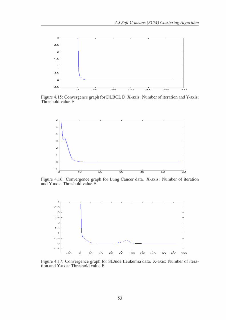
4.3 Soft C-means (SCM) Clustering Algorithm
Figure 4.15: Convergence graph for DLBCL D. X-axis: Number of iteration and Y-axis:Threshold value E
Figure 4.16: Convergence graph for Lung Cancer data. X-axis: Number of iterationand Y-axis: Threshold value E
Figure 4.17: Convergence graph for St.Jude Leukemia data. X-axis: Number of itera-tion and Y-axis: Threshold value E
53

4.4 Comparative studies on Hard C-means and Soft C-means clustering Algorithm
4.4 Comparative studies on Hard C-means and Soft C-means clustering Algorithm
This section deals with comparative studies on Hard C-means and Soft C-means Clus-
tering algorithm. All the fifteen datasets described in section 4.1.1 has been considered
to compare performances of Hard C-means and Soft C-means clustering algorithm.
Table 4.38 shows the result obtained by HCM and SCM clustering algorithm for Iris
data. The total count error in case of HCM clustering algorithm was 17 whereas in case
of SCM, it was 14. The similar result was also reported in literature [46]. Percentage
increase in accuracy for SCM is by 2 %. It may be noted that accuracy of 100 % was
achieved for cluster 1 in HCM as well as in case of SCM. Percentage accuracy is in-
crease by 14 % for cluster 3 in case of SCM.
Table 4.39 shows the result for WBCD data. Percentage increase in accuracy for SCM
is by 0.30% for WBCD. Total count error in case of HCM is 29, whereas in case of
SCM, it is reduced to 27.
Table 4.40 shows the result obtained by HCM and SCM for Serum data (Iyer data). The
data point of one clusters are overlapping with other clusters. This is the reason very
less accuracy was achieved for this datasets. Number of data point correctly clustered
for this datasets is 268 for HCM and 252 for SCM. The optimal value of m was chosen
as 1.92.
Table 4.41 contains the result for Cho data. Percentage accuracy in case of HCM is
60.88 % whereas in case of SCM, it is 63.47 %. Note that percentage accuracy for clus-
ter 4 is increased by 59.26% (i.e., 72.22 - 12.96), whereas for cluster 3 it is decreased
by 26.67%(i.e., 62.67 - 36).
Table 4.42 consists the result for Leukemia data (Golub’s data). Accuracy of 59.72 %
was achieved in case of HCM and 55.56% in case of SCM. It may be noted that cluster
2 is having equal accuracy (44%) in case of HCM as well as in case of SCM. The Golub
et. al.’s microarray datasets is very challenging because the appearance of the two types
of acute Leukemia is highly similar in nature. This was the reason much better accuracy
was not achieved in this case. One probable solution to deal with this problem could
be use dimensionality reduction techniques to reduce the number of features and then
54

4.4 Comparative studies on Hard C-means and Soft C-means clustering Algorithm
subsequently use of SCM clustering algorithm.
Table 4.43 to Table 4.46 consists the result for subtypes of Breast data. As far as Breast
data A is concerned, Number of correctly clustered data point has been raised to 86
(SCM) from 71 (HCM) and therefore percentage accuracy increased by 15.31 %. It may
be noted that in case of SCM, accuracy of 100 % was achieved for cluster 2 whereas
for cluster 1 number of correctly classified data point is zero. In case of Breast data B,
percentage accuracy has been increased by 15.32 (i.e., 87.76-72.44)%. It may be noted
that 100% of accuracy was achieved for cluster 1 and cluster 3 in case of SCM (Breast
data B). In case of Breast multi data A, percentage accuracy is increased by 10.68. It is
important to note that cluster 3 achieve 35.71% accuracy in case of Breast multi data B
whereas in case of SCM it achieved accuracy upto 92.85%.
Table 4.47 to Table 4.50 consists of the result for subtypes of DLBCL Data. As far as
DLBCL A is concerned, increase in accuracy in case of SCM is by 5.67 %. Note that
HCM performs better in case of DLBCL B data. Number of data point correctly clus-
tered in case of HCM is 140 whereas 136 in case of SCM. SCM gives optimal accuracy
when m is 1.285. As far as DLBCL C and DLBCL D are concerned SCM performs
better compared to HCM algorithm on the basis of accuracy parameter. The data of
DLBCL B is of highly distinctively separated in nature compared to other DLBCL (A,
C, D) and that is the reason higher accuracy was achieved in case of DLBCL B. The
reason for inferior performance of SCM compared to HCM for DLBCL B could be
solved by finding a better m value.
Table 4.51 shows the result obtained by HCM and SCM for Lung Cancer data. Overall
accuracy has been raised by 4 % in case of SCM compared to HCM clustering algo-
rithm. It may be observed that accuracy of cluster 3 is 47.62% whereas in case of SCM
it has been raised upto 61.9 %.
Table 4.52 shows the result obtained by HCM and SCM for St. Jude Leukemia data.
The data in this case is of highly separable in nature. As far as HCM is concerned 100
percent accuracy was achieved for cluster 2 whereas in case of SCM 100 % accuracy
was achieved for cluster 2 as well as cluster 6. It may be noted that the least accuracy
was achieved for cluster 5 in HCM as well as in SCM. SCM obtained 16.28 (i,e., 83.72-
55

4.4 Comparative studies on Hard C-means and Soft C-means clustering Algorithm
67.44) % more accuracy compared to HCM algorithm for Cluster 5.
Table 4.37: Comparative study of HCM and SCM using all fifteen dataSl.No.
Datasets #clus-ter
Hard C-means SCM
#Er-ror
Error(%) #cor-rect
Accuracy(%)
mfuz #Er-ror
Error(%)
#cor-rect
Accuracy(%)
% In-creaseIn accu-racy
1 Iris 3 17 11.33 133 88.67 4.2 14 9.33 136 90.67 22 WBCD 2 29 4.25 654 97.75 1.58 27 3.95 656 96.04 .33 Iyer data/Serum
data11 249 48.1624 268 51.84 1.92 265 51.26 252 48.74 -3.1
4 Cho data (yeastdata)
5 151 39.1191 235 60.88 2.15 140 36.27 246 63.73 2.85
5 Leukemia(Golub Experi-ment)
2 29 40.28 43 59.72 1.28 32 44.44 40 55.56 -4.16
6 Breast data A 3 27 27.55 71 72.44 1.6 12 12.25 86 87.75 15.317 Breast data B 4 23 46.93 26 53.06 1.15 17 34.7 32 65.30 12.248 Breast Multi
data A4 21 20.39 82 79.61 1.3 10 9.71 93 90.29 10.68
9 Breast Multidata B
4 15 48.88 17 53.125 1.795 16 50 16 50 -3.125
10 DLBCL A 3 66 46.8085 75 53.191 1.40 58 41.14 83 58.86 5.66911 DLBCL B 3 40 22.22 140 77.78 1.285 44 24.44 136 75.56 -2.2212 DLBCL C 4 28 48.28 30 51.7241 1.345 14 24.14 44 75.86 24.1413 DLBCL D 4 74 57.36 55 42.64 1.25 64 49.62 65 50.38 7.7414 Lung Cancer 4 55 27.92 142 72.0812 1.07 47 23.86 150 76.14 4.0615 St. Jude
Leukemia data6 37 14.91 211 85.08 1.26 29 11.69 219 88.31 3.23
Table 4.38: Comparative study on HCM and SCM for Iris# datapoint
# data pointwrongly clus-tered
# data pointcorrectly clus-tered
Accuracy(%)
HCM Cluster1 50 0 50 100Cluster2 50 4 46 92Cluster3 50 13 37 74Total 150 17 133 88.67
SCM Cluster1 50 0 50 100Cluster2 50 3 47 94Cluster3 50 11 39 88Total 150 14 136 90.67
Table 4.39: Comparative study on HCM and SCM for WBCD# datapoint
# data pointwrongly clus-tered
# data pointcorrectly clus-tered
Accuracy(%)
HCM Cluster1 444 142 302 68.01Cluster2 239 112 127 53.14Total 683 254 429 62.81
SCM Cluster1 444 09 435 97.97Cluster2 239 20 219 91.63Total 683 29 654 95.75
56

4.4 Comparative studies on Hard C-means and Soft C-means clustering Algorithm
Table 4.40: Comparative study of HCM and SCM using Serum Data (Iyer Data)# datapoint
# data pointwrongly clus-tered
# data point cor-rectly clustered
Accuracy(%)
HCM Cluster1 33 17 16 48.48Cluster2 100 84 16 16Cluster3 145 7 138 95.17Cluster4 34 34 0 0Cluster5 43 31 12 27.91Cluster6 7 6 1 14.29Cluster7 34 17 17 50Cluster8 14 1 13 92.86Cluster9 63 28 35 55.56Cluster10 19 12 7 36.84Cluster11 25 12 13 52Total 517 249 268 51.84
SCM Cluster1 33 28 5 15.15
Cluster2 100 6 94 94Cluster3 145 69 84 57.93Cluster4 34 33 1 2.94Cluster5 43 24 19 44.19Cluster6 7 7 0 0Cluster7 34 17 17 50Cluster8 14 14 0 0Cluster9 63 41 22 34.92Cluster10 19 17 2 10.53Cluster11 25 17 8 32Total 517 265 252 48.74
Table 4.41: Comparative study on HCM and SCM for Cho Data)# datapoint
# data pointwrongly clus-tered
# data pointcorrectly clus-tered
Accuracy(%)
HCM Cluster1 67 30 37 55.22Cluster2 135 25 110 81.48Cluster3 75 28 47 62.67Cluster4 54 47 7 12.96Cluster5 55 21 34 61.82Total 386 151 235 60.88
SCM Cluster1 67 15 52 77.62Cluster2 135 55 80 59.3Cluster3 75 48 27 36Cluster4 54 15 39 72.22Cluster5 55 8 47 85.45Total 386 141 245 63.47
Table 4.42: Comparative study on HCM and SCM for Leukemia Data (Golub Expei-ment)
# datapoint
# data pointwrongly clus-tered
# data pointcorrectly clus-tered
Accuracy(%)
HCM Cluster1 47 15 32 68.09
Cluster2 25 14 11 44
Total 72 29 43 59.72
SCM Cluster1 47 18 29 61.702
Cluster2 25 14 11 44
Total 72 32 40 55.56
57

4.4 Comparative studies on Hard C-means and Soft C-means clustering Algorithm
Table 4.43: Comparative study on HCM and SCM for Breast Data A# datapoint
# data pointwrongly clus-tered
# data pointcorrectly clus-tered
Accuracy(%)
HCM Cluster1 11 1 10 90.91
Cluster2 51 22 29 56.86
Cluster3 36 4 32 88.89
Total 98 27 71 72.44
SCM Cluster1 11 11 0 0
Cluster2 51 0 51 100
Cluster3 36 1 35 97.22
Total 98 12 86 87.76
Table 4.44: Comparative study on HCM and SCM for Breast Data B# datapoint
# data pointwrongly clus-tered
# data pointcorrectly clus-tered
Accuracy(%)
HCM Cluster1 12 0 12 100
Cluster2 11 5 6 54.54
Cluster3 7 5 2 28.57
Cluster4 19 13 6 31.58
Total 49 23 26 53.06
SCM Cluster1 12 0 12 100
Cluster2 11 5 6 54.54
Cluster3 7 0 7 100
Cluster4 19 12 7 36.84
Total 49 17 32 65.31
Table 4.45: Comparative study on HCM and SCM for Breast multi data A# datapoint
# data pointwrongly clus-tered
# data pointcorrectly clus-tered
Accuracy(%)
HCM Cluster1 26 2 24 92.31
Cluster2 26 1 25 96.15
Cluster3 28 18 10 35.71
Cluster4 23 0 23 100
Total 103 21 82 79.61
SCM Cluster1 26 5 21 80.77
Cluster2 26 1 25 96.15
Cluster3 28 2 26 92.85
Cluster4 23 2 21 91.3
Total 103 10 93 90.291
58

4.4 Comparative studies on Hard C-means and Soft C-means clustering Algorithm
Table 4.46: Comparative study on HCM and SCM for Breast multi data B# datapoint
# data pointwrongly clus-tered
# data pointcorrectly clus-tered
Accuracy(%)
HCM Cluster1 5 3 2 40
Cluster2 9 2 7 77.78
Cluster3 7 3 4 57.14
Cluster4 11 7 4 36.36
Total 32 15 17 53.13
SCM Cluster1 5 3 2 40
Cluster2 9 3 6 66.67
Cluster3 7 4 3 42.86
Cluster4 11 6 5 45.45
Total 32 16 16 50
Table 4.47: Comparative study on HCM and SCM for DLBCL A# datapoint
# data pointwrongly clus-tered
# data point cor-rectly clustered
Accuracy(%)
HCM Cluster1 49 26 23 46.94Cluster2 50 22 28 56Cluster3 42 18 24 57.14Total 141 66 75 53.19
SCM Cluster1 49 18 31 63.27Cluster2 50 23 27 54Cluster3 42 17 25 59.52Total 141 58 83 58.87
Table 4.48: Comparative study on HCM and SCM for DLBCL B# datapoint
# data pointwrongly clus-tered
# data pointcorrectly clus-tered
Accuracy(%)
HCM Cluster1 42 18 24 57.14Cluster2 51 7 44 86.27Cluster3 87 15 72 82.76Total 180 40 140 77.78
SCM Cluster1 42 13 29 69.05Cluster2 51 16 35 68.63Cluster3 87 15 72 89.66Total 180 44 136 75.56
59

4.4 Comparative studies on Hard C-means and Soft C-means clustering Algorithm
Table 4.49: Comparative study on HCM and SCM for DLBCL C# datapoint
# data pointwrongly clus-tered
# data pointcorrectly clus-tered
Accuracy(%)
HCM Cluster1 17 1 16 94.11Cluster2 16 9 7 43.75Cluster3 13 12 1 7.69Cluster4 12 6 6 50Total 58 28 30 51.72
SCM Cluster1 17 4 13 76.47
Cluster2 16 6 10 62.5Cluster3 13 7 6 46.15Cluster4 12 9 3 25Total 58 26 32 55.17
Table 4.50: Comparative study on HCM and SCM for DLBCL D# datapoint
# data pointwrongly clus-tered
# data pointcorrectly clus-tered
Accuracy(%)
HCM Cluster1 19 13 6 31.58Cluster2 37 28 9 24.32Cluster3 24 13 11 45.83Cluster4 49 20 29 59.18Total 129 74 55 42.64
SCM Cluster1 19 8 11 57.9
Cluster2 37 19 18 48.65Cluster3 24 10 14 58.33Cluster4 49 27 22 44.89Total 129 64 65 50.39
Table 4.51: Comparative study on HCM and SCM for Lung Cancer# datapoint
# data pointwrongly clus-tered
# data point cor-rectly clustered
Accuracy(%)
HCM Cluster1 139 42 97 69.78Cluster2 17 1 16 94.11Cluster3 21 11 10 47.62Cluster4 20 1 19 95Total 197 55 142 72.08
SCM Cluster1 139 36 103 74.1
Cluster2 17 2 15 88.24Cluster3 21 8 13 61.9Cluster4 20 1 19 95Total 197 47 150 76.14
60

4.5 Conclusion
Table 4.52: Comparative study on HCM and SCM for St. Jude Leukemia Data# datapoint
# data pointwrongly clus-tered
# data pointcorrectly clus-tered
Accuracy(%)
HCM Cluster1 15 15 0 0Cluster2 27 0 27 100Cluster3 64 3 61 95.31Cluster4 20 4 16 80Cluster5 43 14 29 67.44Cluster6 79 1 78 98.73Total 248 37 211 85.08
SCM Cluster1 15 15 0 0
Cluster2 27 0 27 100Cluster3 64 3 61 95.31Cluster4 20 4 16 80Cluster5 43 7 36 83.72Cluster6 79 0 79 100Total 248 29 219 88.31
4.5 Conclusion
The SCM based clustering algorithm is a distinct improvement from the conventional
HCM clustering algorithm. Its ability to cluster independent of the data sequence pro-
vides a more stable clustering result. Computer simulation shows that Soft C-means
performs superior compared to Hard C-means algorithm in eleven cases out of fifteen
cases. Datasets belonging to these cases are Iris, WBCD, Yeast (Cho) data, Breast Data
(A, B), Breast multi data A, DLBCL (A,C,D), Lung Cancer and St. Jude leukemia.
Whereas Hard C-means shows superior performance in four cases. Datasets belonging
to these cases are serum data, leukemia data, Breast multi data B and DLBCL B. As
seen from the experiments, the SCM based clustering algorithm was able to provide the
highest accuracy and generalization results.
61

Chapter 5
Genetic Algorithm based ClustreingAlgorithm
Clustering can be formally formulated as a NP-hard grouping problem from optimiza-
tion perspective [102]. This research finding has stimulated the search for efficient
approximation algorithms, including not only the use of ad-hoc heuristics for particu-
lar classes or instances of problems, but also the use of general-purpose metaheuristics
[103]. Particularly, evolutionary algorithms are metaheuristics widely believed to be
effective on NP-hard problems, being able to provide near-optimal solutions to such
problems in reasonable time. Under this assumption, a large number of evolutionary al-
gorithms for solving clustering problems have been proposed in the literature . A useful
review on this can be found from review paper [34]. These algorithms are based on the
optimization of some objective function (i.e., the so-called, fitness function) that guides
the evolutionary search. In evolutionary algorithm, Genetic Algorithm (GA) becomes
natural choice for cluster formation algorithm due to its wide applicability in wide range
of areas.
GA is inspired by Darwin’s theory of evolution. A GA works with a population of in-
dividuals each of which represents a potential solution to the problem to be solved. A
typical individual is a binary string on which the problem solution is encoded. Problem
representation is one of the key decision to be made when applying a GA to a prob-
lem. Problem representation in a GA individual determines the shape of the solution
space, that a GA must search. As a result, “different encodings of the same problem
are essentially different problems for a GA” [104]. The application of GAs for solving
problems of pattern recognition appears to be appropriate and natural. A number of
62

research articles in this area have started to come out [105], [106], [107], [108], [109],
[110], [111], [112], [113], [114]. An application of GAs has been reported in the area of
(supervised) pattern classification for designing a GA-classifier [107], [115]. GA based
Clustering algorithm for machine learning data has been also reported in literature [17],
[116], [117], [118]. The paper [17] was the referenced which motivated us to work on
GA based clustering algorithm.
In the paper [17], extensive studies has been done on wide variety of artificial and
real-life data. These datasets having both overlapping and non-overlapping class bound-
aries. Paper [17] discusses binary as well as multi-class classifier problem (unsuper-
vised). The paper [17] is specific to pattern recognition data. Mean square error (MSE)
has been used as fitness function in paper [17]. In paper [17], chromosome representa-
tion is based on cluster center which is made up of features of the data point (i.e., gene).
When no. of features considered are large e.g., microarray data, length of the chromo-
some becomes very large if chromosome representation was followed based on paper
[17]. In such cases it is advisable to go for some alternative means of chromosome
representation e.g., based on instances i.e., data point itself instead of going for fea-
ture based representation. The paper [17] is specific to pattern recognition data. There
are no work reported in literature for bioinformatics data specially for microarray data
using GA. In this chapter of the thesis, study has been made on Family of GA based
clustering algorithm to bioinformatics data. Bioinformatics data possess some charac-
teristics feature which machine learning data do not possess. Microarray data possesses
a number of features (generally, in range of 103 − 104) very large compared to pattern
recognition data.
In this thesis, along with paper [17], three different representation schemes for GA
based clustering was studied. This chapter of the thesis deals with machine learning
data as well as bioinformatics data having overlapping and non-overlapping clusters.
The data belongs to binary as well as multi class problem. It also deals with problem
like clusters within a clusters (i.e., subtypes of a cluster). Binary representation (SGA-
simple Genetic Algorithm) as well as floating-point representation (RGA-Real coded
Genetic Algorithm) has been considered for GA. It is important to note that efficiency
63

5.2 Basic Steps involved in GA based Clustering
of a GA based algorithm mainly depends on two factors; first representation scheme
and fitness function computation [137], [138]. Depending upon chromosome represen-
tation schemes crossover and mutation operator was modified. The way chromosome
was represented and novel fitness function was used in this thesis makes it different
from previous approaches and results in an efficient clustering algorithm.
5.1 Basic principle
The searching capability of GAs [139] has been used in this chapter of the thesis for
cluster formation of ‘n’ data points where labeled information are not available at
the time of cluster formation. This has been achieved using either determining 1):
Data point belonging to each cluster i.e., {V1,V2. . . . ,VC} or 2): Cluster center i.e.,
{v1,v2. . . . ,vC} in problem solution space RN ; where ‘C’ is a fixed number of clus-
ter given by user. The fitness function that has been adopted is the HS Ratio of the
cluster. HS Ratio has been discussed in detail in section 5.2.3.
The objective of the GA is to search for the appropriate 1:) Cluster i.e., {V1,V2. . . . ,VC}or 2): Cluster center i.e, {v1,v2. . . . ,vC}; such that fitness function ‘ f ’ is minimized.
5.2 Basic Steps involved in GA based Clustering
The basic steps of GAs (shown in fig. 5.1); which are also followed in the GA-clustering
algorithm, are now described in details in this section.
Initially, a random population is created, which represents different data point in a clus-
ter or cluster center in the problem search space. Then fitness value of each chromosome
is computed. Based on the principle of survival of the fittest, a few of the chromosome
are selected and each is assigned a number of copies that go into the mating pool. Then
crossover operator are applied on these string and that results in set of crossover chil-
dren. Next, mutation was applied on the crossover children that results set of mutated
children. parent chromosome, crossover children and mutated children yields set of
chromosome for the new generation. The process of selection, crossover and mutation
continues for a fixed number of generation or till a termination condition is satisfied.
In this section; discussion has been made on four different representation schemes for
64

5.2 Basic Steps involved in GA based Clustering
Figure 5.1: Flow chart of simple GA
65

5.2 Basic Steps involved in GA based Clustering
encoding of a chromosome.
5.2.1 Encoding of Chromosome
1. Representation 1 (GA-R1):
This representation is based on number of data points. In this representation; each
chromosome is represented by a sequence of binary numbers representing the
clusters. For ‘n’ data-point of N-dimensional space and ‘C’ number of clusters,
the length of a Chromosome will be ‘n×C’ word length, where the first ‘n’ word
length represents the first cluster, the next ‘n’ word length represents those of the
second cluster, and so on. It may be noted that in a cluster if a word position is
‘1’ (It is said to be in ON state), it means that the data point is present and ‘0’ (it
is said to be in OFF state) means data point is absent. As an illustration for the
above representation, let us consider the following example.
Example 1.
Let us consider Iris data [150 x 4], where n=150, N=4 and C=3, i.e., the space
is four dimensional and the number of clusters being considered is three. There-
fore, the size of the Chromosome will be 450 (i.e., n×C). Then the Chromo-
some/String representation will be as follows:
Encoding of chromosome using representation 1
First Cluster Second Cluster Third Cluster
1 0 0 0 0 1 . . . upto 150 bits 0 1 1 0 0 0 . . . upto 150 bits 0 0 0 1 1 0 . . . upto 150 bits
According to above chromosome representations: since in first cluster index 1
and 6 are one. Therefore, Data point ‘1’ and Data point ‘6’ are present in First
Cluster. Similarly, Second Cluster contains Data point ‘2’ and Data point ‘3’,
Third Cluster contains Data point ‘4’ and Data point ‘5’, and so on.
2. Representation 2 (GA-R2):
This representation is based on cluster center (i.e., number of features). In this
representation; each Chromosome is represented by a sequence of real numbers
representing the centers of ‘C’ clusters. For ‘n’ data-point of N-dimensional
66

5.2 Basic Steps involved in GA based Clustering
space, the length of a Chromosome will be ‘N×C’ word length, where the first
‘N’ positions (or, features) represent the ‘center o f f irst cluster‘, next ‘N’ po-
sitions represent those of the ‘center o f second cluster‘, and so on. It may be
noted that cluster center is of N-dimensional space. This representation is similar
to paper [17]. As an illustration for the above representation, let us consider the
following example.
Example 2.
Consider the same Iris data again. The size of the Chromosome in this case will
be twelve (i.e., N×C = 12). Then the Chromosome/String representation will
be:
Encoding of chromosome using representation 2
Center of First Cluster Center of Second Cluster Center of Third Cluster
5.2 4.1 1.5 0.1 5.3 3.7 1.5 0.2 5.7 2.9 4.2 1.3
3. Representation 3 (GA-R3):
This representation is extension of ‘Representation 2’. This involves two step:
In first step, a chromosome is represented as stated in Representation 2 and in
second step; each word of first step representation is represented by a sequence
of binary length of specified length (say, ‘nw’). The minimum value of ‘nw’ is
equal to size of binary number required to represent the maximum value of a
feature in original data.
Example 3: Consider the same Iris data again. In first step, a chromosome will be
size of 12 word length (according to Representation 2). Here each word (feature)
is represented by a real number. In the second step, each word of representa-
tion 2 is represented by a sequence of binary number of specified word length.
Let us take 10 word length to represent one word (i.e., one feature) of first step
representation. Therefore the resultant length of a Chromosome after second rep-
resentation will be of ‘120’ word length (i.e., 3× 4× 10 = 120). Then the
Chromosome/String representation will be :
Consider the Center of First Cluster
67

5.2 Basic Steps involved in GA based Clustering
Encoding of chromosome using representation 3
Center of First Cluster Center of Second Cluster Center of Third Cluster
1 0 0 0 0 1 . . . Upto 40 bits 0 1 1 0 0 0 . . . Upto 40 bits 0 0 0 1 1 0 . . . Upto 40 bits
Complete view of first cluster of chromosome using representation 3
1 1 1 1 0 0 0 0 1 1 1 1 1 1 1 0 0 0 0 0 0 0 0 0 0 1 1 1 1 1 1 1 0 0 1 1 0 0 1 1
First block of the first cluster (i.e. first 10 bits of the first cluster) represents one
gene i.e., the feature number one i.e. first dimension of center of first cluster.
4. Representation 4 (GA-R4):
This representation is combination of Representation 1 and Representation 3. In
first step, chromosome is represented as stated in representation 1. Hence for
Iris data, the size of chromosome in first step will be 450 (i.e., 3× 150). It’s a
binary representation. Here if a bit is found to be ‘1‘, it means a data point is
present in the cluster otherwise the data point is absent in the cluster. Now for
each cluster, center (or, mean) was computed. Since center’s of each cluster is of
dimension four. So now the size of chromosome will be of size 12 (i.e., 3× 4).
In the next step, each feature of cluster’s center is represented by binary sequence
of specified length (say, 10) as stated in Representation 3. So the size of resultant
chromosome will be 120 (i.e., 3×4×10 = 120) word (or, bit) length. Then the
Chromosome/String representation will be:
Encoding of chromosome using representation 4
First Cluster Second Cluster Third Cluster
1 0 0 0 0 1 . . . Upto 40 bits 0 1 1 0 0 0 . . . Upto 40 bits 0 0 0 1 1 0 . . . Upto 40 bits
It is important to note that Representation 4 is equivalent to ‘representation 3’;
but the way it is derived i.e., the meaning is different. Hence the simulation result
obtained for this two representation will be same if the randomly initial popula-
tion (i.e., cluster) generated are same. For this reason the discussion has been
made on the simulation result obtained by representation 3 only in this chapter.
68

5.2 Basic Steps involved in GA based Clustering
5.2.2 Population initialization
The ‘C’ number of clusters encoded in each chromosome are initialized as stated in
Encoding of chromosome (Section 5.2.1). The chromosome initialization can be done
either randomly or by using any greedy or intelligent method. This process is repeated
for each of the ‘P’ chromosome in the population, where ‘P’ is the size of the popula-
tion.
5.2.3 Fitness Evaluation of Chromosome
This is the one of the most important part of proposed approach. The fitness function
evaluation is based on Homogeneity and separation value. It is based on the principle
“objects within one cluster are assumed to be similar to each other, while objects in
different clusters are dissimilar”. Fitness computation process consists of two steps:
in first step, Homogeneity value and Separation value is calculated. In second step,
HS Ratio is defined as ratio of homogeneity to separation.
The homogeneity of a cluster V is defined as follows ([20], [45]):
H1(V ) =∑Ei, E j∈V, Ei 6=E j Similarity
(Ei , E j
)
‖V ‖.(‖V ‖ −1)
This definition represents the homogeneity of cluster V by the average pair-wise object
similarity within V.
Cluster separation is analogously defined from various perspectives to measure the dis-
similarity between two clusters V1,V2 ([20], [45]). For example:
S1(V1,V2) =∑Ei∈V1, E j∈V2 Similarity
(Ei , E j
)
‖V1 ‖.(‖V2 ‖)Since these definitions of homogeneity and separation are based on the similarity be-
tween objects, the quality of V increases with higher homogeneity values within V and
lower separation values between V and other clusters. Once homogeneity of a cluster
and the separation between a pair of clusters has been defined, for a given clustering
result {V1,V2, . . . ,VC}, Then average homogeneity and the average separation of V can
be defined. For example, Shamir et al. [20] used definitions of
Haverage =∑Vi∈V ‖Vi ‖ .H1(Vi)
N
69

5.2 Basic Steps involved in GA based Clustering
and
Saverage =1
∑Vi 6=V j ‖Vi ‖ . ‖V j ‖ ∑Vi 6=V j
‖Vi ‖ . ‖V j ‖.S1(V1,V2)
to measure the average homogeneity and separation for the set of clustering results V.
The HS Ratio is defined as : HS Ratio = HaverageSaverage
. The fitness function J for a chromo-
some is defined as: J = 1/HS Ratio. Here objective is to minimize fitness function
J.
5.2.4 Selection
The selection step in GA, selects chromosome from the mating pool and follows “the
survival of the fittest” concept of Darwin’s natural genetic system. In this chapter,
a proportional selection strategy has been adopted. Roulette Wheel selection is one
common technique that implements the proportional selection strategy. According to
this, a chromosome is being assigned with a number of copies, which is proportional to
its fitness in the population that goes into the mating pool for further genetic operations
[139].
5.2.5 Crossover
It is a type of genetic operations, which is used to create new child chromosome from
parent chromosome after exchanging information between them. It is based on proba-
bilistic model. Several variants of Cross-over has been discussed in past [139]. In this
thesis, a single-point crossover with a fixed crossover probability ‘Pc’ is used. For chro-
mosome of length ‘cs’, a random integer ‘cp’, called the crossover point, is generated in
the range [2, cs-1]. The portions of the chromosome lying to the right of the crossover
point are exchanged to produce two offspring. It is important to note that depending
upon the representation schemes of chromosome in GA crossover operation changes.
GA-R2 and GA-R3 follows crossover as stated above whereas in case of GA-R1, after
doing the crossover as stated above, a post processing is required. Details about this
post processing is explained below:
1. Crossover in GA-R1
Let us consider a dataset having ten data points of two dimension and number
70

5.2 Basic Steps involved in GA based Clustering
of cluster is two. According to GA-R1, chromosome representation will be as
follows:
Chromosome 1 1 0 1 0 1 0 0 0 1 1 0 1 0 1 0 1 1 1 0 0Chromosome 2 0 0 1 1 1 0 1 1 0 0 1 1 0 0 0 1 0 0 1 1
crossover point ‘cp’ is 10. Then chromosome after crossover will look like as
follows:
Crossover children 1 (Chromosome) 1 0 1 0 1 0 0 0 1 1 1 1 0 0 0 1 0 0 1 1
Crossover children 2 (Chromosome) 0 0 1 1 1 0 1 1 0 0 0 1 0 1 0 1 1 1 0 0
Now let us consider crossover children 1; cluster 1 contains data point {1 3 5 9
10} and cluster 2 contains data point {1 2 6 9 10}. It may be noted that crossover
children’s ’1’ do not follow definition of clustering defined in section 2.2.1. data
points {1 9 10} appear in both the cluster and data points {4, 7, 8} is missing
in chromosome (crossover children 1) i.e., these data point do not belong to any
cluster. To sort out this problem, post processing is required for each and every
crossover children and it is done as follows:
Select any cluster in a chromosome randomly and fix that as a true cluster and
make changes to other cluster such that it follows definition of clustering.
For illustration, consider crossover children 1 as an example. select any cluster
randomly out of available two clusters. say cluster 1 has been chosen. Make
this as true cluster and do processing in cluster 2 in such a way that it follows
definition of clusters. After processing, crossover children 1 look like as follows:
Crossover children 1 (Chromosome) 1 0 1 0 1 0 0 0 1 1 0 1 0 1 0 1 1 1 0 0
After post processing, cluster 1 contains data point {1 3 5 9 10} and cluster 2
contains data point {2 4 6 7 8} which follows definition of clustering.
5.2.6 Mutation
It is a type of genetic operator that alters one ore more gene values in a chromosome
from its initial state. This can result in entirely new gene values being added to the gene
71

5.3 Experimental Setup
pool. With these new gene values, the genetic algorithm may be able to arrive at better
solution than was previously possible. Mutation is an important part of the genetic
search as help helps to prevent the population from stagnating at any local optima.
Each chromosome in a population undergoes mutation with a fixed probability, ‘Pm’.
For binary representation of a chromosome (GA-R1 and GA-R3), mutation is done by
flipping its bit position (or gene) value i.e. if a bit position is 1 it is made 0 and vice
versa. A bit position in GA-R1 represents weather a data point is present in a cluster
or not whereas in a GA-R3 it represents a position of cluster center. It is important to
note that GA-R1 requires post processing as similar to how it has been done in case of
crossover, whereas GA-R3 does not require any processing after mutation. For floating-
point representation in GA-R2, mutation was done as follows [17] : A random number
η in the range [0, 1] is generated with uniform distribution. If the value at a gene
position is ‘ν’, after mutation, it becomes ν×(1+ 2×η). One may note in this context,
that similar sort of mutation operators for real coding have been used mostly in the realm
of evolutionary strategies [17].
5.2.7 Termination criterion
In this chapter the processes of fitness computation, genetic operation is executed for a
maximum number of iterations.
In the next section, GA based clustering algorithm has been discussed for machine
learning data as well as bioinformatics data.
5.3 Experimental Setup
To validate the feasibility and performance of the GA based clustering algorithm, clus-
tering accuracy was used as cluster validation metric. Since the data possess class label
information. Clustering accuracy is defined as follows:
Clustering Accuracy = ( Number o f Correct CountTotal number o f instances genes/samples) × 100.
Simulation studies has been carried out in MATLAB 7.0 (Intel C2D processor, 2.0
GHz, 2 GB RAM) and applied it to machine learning data as well as to bioinformatics
data. For simplicity, this section is divided into two subsection. First section contains
the details result obtained on machine learning data using GA clustering algorithm and
72

5.3 Experimental Setup
second section contains detailed result obtained for bioinformatics data using the same
algorithm.
5.3.1 Experiment 1: Machine Learning Data
In this section, discussion has been made on Family of GA based Clustering algorithm to
two machine learning data i.e., Iris and WBCD. The details of these two data have been
already explained in section 4.1.1. Comparison has been done on proposed GA based
clustering algorithm with following five standard conventional Clustering algorithm [9]
for Iris data:
1. Hierarchical Clustering
2. Self Organizing Map based (SOM) Clustering
3. Hard C-means Clustering
4. Generalized Linear Vector Quantization (GLVQ) Clustering
5. Soft C-means (SCM) Clustering
5.3.2 Results and Discussion
The parameters used for Iris and WBCD data in GA based clustering algorithm is shown
in Table 5.1.
Complete result of GA based clustering algorithm for machine learning and bioinfor-
matics data has been given in appendix F. Appendix F contains the details of data point
wrongly clustered in GA clustering algorithm. From this, It can be deduce about details
of data point correctly clustered in each cluster and subsequently distribution of data
point after simulation of cluster formation algorithm. Here in this section, result ob-
tained for GA based clustering algorithm for machine learning data has been presented
in brief.
Table 5.2 summarizes result of nine clustering algorithm (5 conventional and 4 GA
based clustering) for Iris data. Here best case analysis has been considered for four
representation schemes used for GA based clustering algorithm. It may be noted that
“for Iris data a clustering algorithm which gives less than 18 count errors considered
73

5.3 Experimental Setup
to be a good clustering algorithm” [46], [47], [49], [48]. Count error was achieved in
the range {0 – 10} for GA-clustering Algorithm. It can be easily infer from Table 5.2
that GA based clustering algorithm performs better than all other algorithm for Iris data.
GA-R1 achieves accuracy upto 93.33 % and GA-R2 achieves accuracy upto 96%. It is
important to note that GA-R3 clustering algorithm can achieve 100 percent accuracy in
its best case analysis. It can be easily infers from the Table 5.2 that GA based clustering
algorithm performs better than other non-GA based clustering algorithm for Iris data.
Table 5.3 describes the result obtained by GA-R1. It shows the initial cluster distribu-
tion (randomly taken from initial population) as well as final cluster distributions after
simulation. Total count error was achieved as 10 and therefore percentage accuracy as
93.33%.
Table 5.4 describes the details of result obtained by GA clustering algorithm. It contains
following information:
the total number of data points in each cluster in a data, number of data point wrongly
clustered, number of data point correctly clustered, details of data point wrongly clus-
tered, individual accuracy of each cluster as well as over all accuracy for GA-R1 for Iris
data. Here clustering accuracy result for Iris-setosa is 100 percent, whereas in case of
Iris-versicolor and Iris-virginica data, number of data points wrongly clustered is 1 and
9 respectively. Datapoint {78} which should be in Iris-versicolor is wrongly clustered
into Iris-virginica and data-point {102, 107, 114, 120, 122, 134, 139, 143, 147} which
should be in Iris-virginica is wrongly classified into Iris-versicolor.
Table 5.5 show the details of the cluster obtained before and after GA run. Table 5.6
describes the result obtained by GA-R2 based genetic algorithms. Count error has
been obtained as 6. Accuracy of 100 % was achieved for cluster Iris-setosa and Iris-
versicolor, whereas for Iris-virginica 88% accuracy was achieved. The wrongly clus-
tered data points are {101, 102, 103, 104, 105, and 107}. In actual practice, all these
data points belong to Iris-virginica, but they have wrongly clustered into Iris-versicolor.
Another very important point to be noted is that data point {102, 107} is wrongly clus-
tered by both representation R1 and R2. These data point are highly non-separable.
Data point 102 is having feature value {5.8, 2.7, 5.1, 1.9} and Data point 107 is having
74

5.3 Experimental Setup
feature value {4.9, 2.5, 4.5, 1.7}; these data points which are in Iris-virginica are hav-
ing value similar to data point belonging to Iris-versicolor. This is the reason these data
points are wrongly classified/clustered by many algorithm in the literature [47], [49].
Table 5.7 describes the result obtained by representation 3 based genetic algorithms. It
shows the details of the generated cluster before as well as after GA run. In this 100%
accuracy was achieved.
GA based clustering algorithm (i.e., GA-R1, GA-R2 and GA-R3) was simulated 20
times. Summary of results obtained after simulation has been shown in Table 5.8.
Table 5.1: Parameter used in GA based clustering Algorithm for Pattern recognitiondata
Parameter ValuePopulation Size 10 - 100Maximum No. Of Iteration 15 - 50Crossover Probability 0.6 - 0.8Mutation Probability 0.001 - 0.01
Table 5.2: Comparison of Results for nine clustering algorithm using Iris DataAlgorithm Count Error Percentage error Percentage
AccuracyHierarchical 48 32 68SOM 22 14.67 85.33HCM 17 11.33 88.67GLVQ 16 10.76 89.33SCM 14 9.33 90.67GA(Representation 1) 10 6.67 93.33GA(Representation 2) 6 4 96GA(Representation 3) 0 0 100GA(Representation 4) 0 0 100
Table 5.3: Initial and final cluster distribution for GA-R1 for Iris DataInitial cluster
Cluster 1 Cluster 2 Cluster 31 2 3 4 5 6 7 8 9 10 11 12 13 1415 16 17 18 19 20 21 22 23 24 2526 27 28 29 30 31 32 33 34 35 3637 38 39 40 41 42 43 44 45
53 78 101 103 104 105 106 108109 110 111 112 113 116 117 118119 121 123 125 126 129 130 131132 133 135 136 137 138 140 141142 144 145 146 148 149
51 52 54 55 56 57 58 59 60 61 62 63 6465 66 67 68 69 70 71 72 73 74 75 76 7779 80 81 82 83 84 85 86 87 88 89 90 9192 93 94 95 96 97 98 99 100 102 107114 115 120 122 124 127 128 134 139143 147 150
Final ClusterCluster 1 Cluster 2 Cluster 31 2 3 4 5 6 7 8 9 10 11 12 13 1415 16 17 18 19 20 21 22 23 24 2526 27 28 29 30 31 32 33 34 35 3637 38 39 40 41 42 43 44 45 46 4748 49 50
51 52 53 54 55 56 57 58 59 60 6162 63 64 65 66 67 68 69 70 71 7273 74 75 76 77 79 80 81 82 83 8485 86 87 88 89 90 91 92 93 94 9596 97 98 99 100
101 103 104 105 106 108 109 110 111112 113 115 116 117 118 119 121 123124 125 126 127 128 129 130 131 132133 135 136 137 138 140 141 142 144145 146 148 149 150
Count error= 10Accuracy = 93.33 %
75

5.3 Experimental Setup
Table 5.4: Result of GA-R1 using Iris DataIris-setosa
Iris-versicolor
Iris-virginica Total
The right number of data point 50 50 50 150Details of Data points wronglyclustered
NIL 78 102 107 114 120 122134 139 143 147
78 102 107 114 120 122134 139 143 147
number of data point wronglyclustered
0 1 9 10
number of data point correctlyclustered
50 49 41 140
Accuracy (%) 100 98 82 93.33
Table 5.5: Initial and final cluster distribution for GA-R2 for Iris DataInitial cluster
Cluster1 Cluster2 Cluster31 2 5 11 13 17 21 22 25 29 32 35 39 4445 50 59 60 61 71 72 73 74 75 76 7778 79 86 90 98 99 46 49 121 122 123124 125 126 127 128 129 130 131 132133 134 140 141 142 143
3 4 6 7 15 16 18 24 26 30 33 34 36 4042 51 52 53 54 55 56 57 58 80 81 8287 88 89 92 93 95 96 97 100 101 102103 104 105 106 107 144 145 146 147148 149 150
8 9 10 12 14 19 20 23 27 28 31 37 3841 43 47 48 62 63 64 65 66 67 68 6970 83 84 85 91 94 108 109 110 111112 113 114 115 116 117 118 119 120135 136 137 138 139
Final ClusterCluster1 Cluster2 Cluster31 2 3 4 5 6 7 8 9 10 11 12 13 14 15 1617 18 19 20 21 22 23 24 25 26 27 2829 30 31 32 33 34 35 36 37 38 39 4041 42 43 44 45 46 47 48 49 50
51 52 53 54 55 56 57 58 59 60 61 6263 64 65 66 67 68 69 70 71 72 73 7475 76 77 78 79 80 81 82 83 84 85 8687 88 89 90 91 92 93 94 95 96 97 9899 100 101 102 103 104 105 107
106 108 109 110 111 112 113 114 115116 117 118 119 120 121 122 123 124125 126 127 128 129 130 131 132 133134 135 136 137 138 139 140 141 142143 144 145 146 147 148 149 150
Count error=6Accuracy = = 96 %
Table 5.6: Result of GA-R2 using Iris DataIris-setosa Iris-
versicolorIris-virginica Total
The right number of data point 50 50 50 150Details of Data points wronglyclustered
NIL NIL 101 102 103 104105 107
101 102 103 104 105107
number of data point wronglyclustered
0 0 6 6
The number of data point cor-rectly clustered
50 50 44 144
Accuracy (%) 100 100 88 96
76
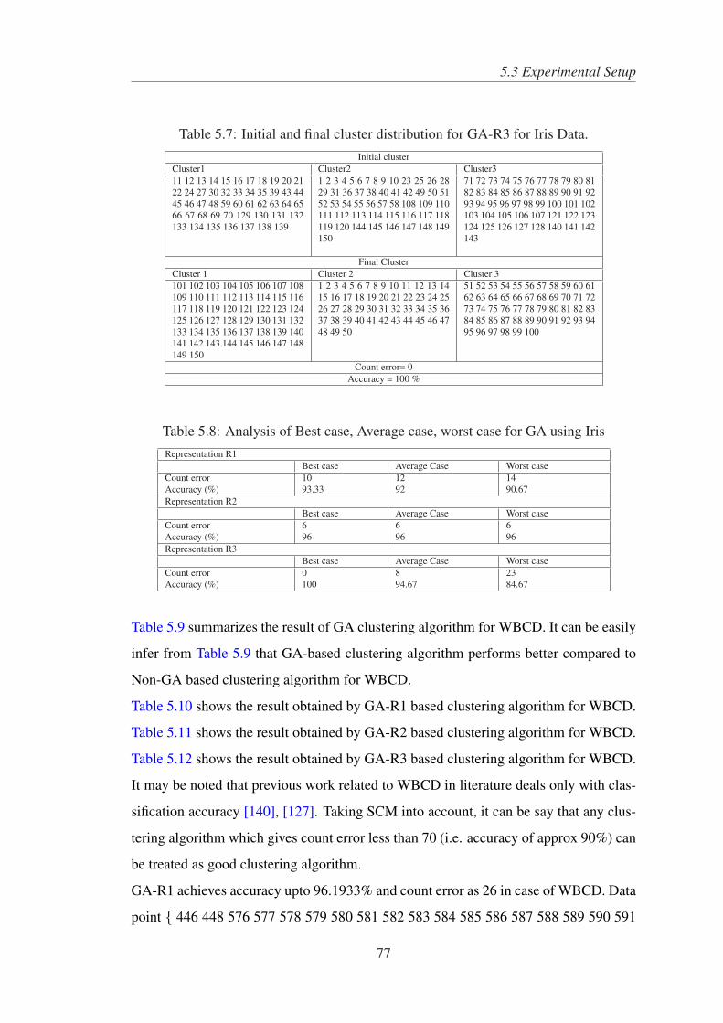
5.3 Experimental Setup
Table 5.7: Initial and final cluster distribution for GA-R3 for Iris Data.Initial cluster
Cluster1 Cluster2 Cluster311 12 13 14 15 16 17 18 19 20 2122 24 27 30 32 33 34 35 39 43 4445 46 47 48 59 60 61 62 63 64 6566 67 68 69 70 129 130 131 132133 134 135 136 137 138 139
1 2 3 4 5 6 7 8 9 10 23 25 26 2829 31 36 37 38 40 41 42 49 50 5152 53 54 55 56 57 58 108 109 110111 112 113 114 115 116 117 118119 120 144 145 146 147 148 149150
71 72 73 74 75 76 77 78 79 80 8182 83 84 85 86 87 88 89 90 91 9293 94 95 96 97 98 99 100 101 102103 104 105 106 107 121 122 123124 125 126 127 128 140 141 142143
Final ClusterCluster 1 Cluster 2 Cluster 3101 102 103 104 105 106 107 108109 110 111 112 113 114 115 116117 118 119 120 121 122 123 124125 126 127 128 129 130 131 132133 134 135 136 137 138 139 140141 142 143 144 145 146 147 148149 150
1 2 3 4 5 6 7 8 9 10 11 12 13 1415 16 17 18 19 20 21 22 23 24 2526 27 28 29 30 31 32 33 34 35 3637 38 39 40 41 42 43 44 45 46 4748 49 50
51 52 53 54 55 56 57 58 59 60 6162 63 64 65 66 67 68 69 70 71 7273 74 75 76 77 78 79 80 81 82 8384 85 86 87 88 89 90 91 92 93 9495 96 97 98 99 100
Count error= 0Accuracy = 100 %
Table 5.8: Analysis of Best case, Average case, worst case for GA using IrisRepresentation R1
Best case Average Case Worst caseCount error 10 12 14Accuracy (%) 93.33 92 90.67Representation R2
Best case Average Case Worst caseCount error 6 6 6Accuracy (%) 96 96 96Representation R3
Best case Average Case Worst caseCount error 0 8 23Accuracy (%) 100 94.67 84.67
Table 5.9 summarizes the result of GA clustering algorithm for WBCD. It can be easily
infer from Table 5.9 that GA-based clustering algorithm performs better compared to
Non-GA based clustering algorithm for WBCD.
Table 5.10 shows the result obtained by GA-R1 based clustering algorithm for WBCD.
Table 5.11 shows the result obtained by GA-R2 based clustering algorithm for WBCD.
Table 5.12 shows the result obtained by GA-R3 based clustering algorithm for WBCD.
It may be noted that previous work related to WBCD in literature deals only with clas-
sification accuracy [140], [127]. Taking SCM into account, it can be say that any clus-
tering algorithm which gives count error less than 70 (i.e. accuracy of approx 90%) can
be treated as good clustering algorithm.
GA-R1 achieves accuracy upto 96.1933% and count error as 26 in case of WBCD. Data
point { 446 448 576 577 578 579 580 581 582 583 584 585 586 587 588 589 590 591
77

5.3 Experimental Setup
592 593 594 600} which are Benign, are wrongly clustered into Malignant, whereas
data points {2 4 139 244} are malignant in nature, but are wrongly clustered into Be-
nign.
GA-R2 achieves accuracy upto 96.7789% and count error in this case obtained to be
37. Data point { 2 4 139 244} which are Benign, are wrongly clustered into Malignant
whereas data points {446 448 576 577 578 579 580 581 582 583 584 585 586 587 588
589 590 591 592 593 594} which are malignant in nature are wrongly clustered into
Benign.
Final fitness value of GA based clustering algorithm for five run has been tabulated in
Table 5.13 and Table 5.14 for Iris and WBCD respectively.
Table 5.15 consists of the optimal fitness value for Iris and WBCD data for GA-R1,
GA-R2 and GA-R3 based clustering algorithms.
Table 5.9: Comparison of clustering algorithm for WBCDAlgorithm Count Error Percentage error Percentage
AccuracyHCM 29 4.2460 95.7540SCM 27 3.9531 96.0469GA(Representation 1) 26 657 96.1933GA(Representation 2) 22 661 96.7789GA(Representation 3) 18 665; 97.3646
Table 5.10: Result of GA-R1 using WBCDBenign Malignant Total
The right number ofdata point
444 239 683
Details of Data pointswrongly clustered
2 4 139 244 446 448 576 577 578 579 580581 582 583 584 585 586 587588 589 590 591 592 593 594600
2 4 139 244 446 448 576 577578 579 580 581 582 583 584585 586 587 588 589 590 591592 593 594 600
number of data pointwrongly clustered
4 22 26
The number of datapoint correctly clus-tered
441 217 657
Accuracy (%) 99.324 90. 8 98.83
78

5.3 Experimental Setup
Table 5.11: Result of GA-R2 using WBCD
Benign Malignant Total
The right number of datapoint
444 239 683
Details of Data pointswrongly clustered
NIL 446 448 576 577 578 579 580581 582 583 584 585 586 587588 589 590 591 592 593 594600
446 448 576 577 578 579 580581 582 583 584 585 586 587588 589 590 591 592 593 594600
number of data pointwrongly clustered
0 22 22
The number of data pointcorrectly clustered
444 217 661
Accuracy (%) 100 88.93 96.78
Table 5.12: Result of GA-R3 using WBCD
Benign Malignant Total
The right number ofdata point
444 239 683
Details of Data pointswrongly clustered
NIL 446 448 580 581 582 583 584585 586 587 588 589 590 591592 593 594 600
446 448 580 581 582 583 584585 586 587 588 589 590 591592 593 594 600
number of data pointwrongly clustered
0 18 18
The number of datapoint correctly clus-tered
444 221 665
Accuracy (%) 100 92.5 97.36
Table 5.13: Fitness Function values for different Run for Iris data.
Trial No. Iris Data
GA-R1 GA-R2 GA-R3
1 0.0099 0.0109 0.0103
2 0.0099 0.0109 0.0103
3 0.0097 0.0109 0.0099
4 0.0099 0.0103 0.0101
5 0.0099 0.0109 0.0103
79

5.3 Experimental Setup
Table 5.14: Fitness Function values for different Run for WBCD data.
Trial No. WBCD Data
GA-R1 GA-R2 GA-R3
1 0.00171 0.00173 0.00170
2 0.00171 0.00173 0.00170
3 0.00167 0.00173 0.00158
4 0.00167 0.00173 0.00158
5 0.00158 0.00173 0.00158
Table 5.15: Final Fitness Function value for machine learning DataDatasetSl.No.
Datasets GA-R1 GA-R2 GA-R3
1 Iris 0.0097 0.0103 0.0101
2 WBCD 0.00158 0.00173 0.00158
5.3.3 Experiment 2: Bioinformatics Data
In this section, discussion has been made on Family of GA based Clustering algorithm
to all the bioinformatics data stated in section 4.1.1. Thirteen microarray data has been
considered for simulation studies. These data are: Iyer data/Serum data, Cho data (yeast
data), Leukemia (Golub Experiment), Breast data A, Breast data B, Breast Multi data
A, Breast Multi data B, DLBCL A, DLBCL B, DLBCL C, DLBCL D, Lung Cancer,
St. Jude Leukemia data. The details of these data has been already explained in section
4.1.1. Complete result of GA Clustering result for each individual bioinformatics data
is given in appendix F.
5.3.4 Results and Discussion
The parameters used for GA based clustering algorithm for Bioinformatics data is
shown in Table 5.16
Table 5.17 to Table 5.29 shows the result obtained by GA-R1 for bioinformatics data.
All these data contains the following information of GA-R1 for bioinformatics data:
80

5.3 Experimental Setup
the right number of data point in each cluster, details of data points wrongly clustered
in each cluster, number of data points in each cluster, number of data point correctly
clustered in each cluster and individual accuracy of each cluster of a data as well as
overall accuracy for each bioinformatics data.
Table 5.17 contains the result obtained by GA-R1 for Breast Data A. Number of data
point wrongly clustered in cluster 1 is one, in cluster 2 is six and in cluster 3 is three.
The total number of data points wrongly clustered is ten. Details of the data point
wrongly clustered are {11 20 31 38 39 46 56 66 80 81}. The overall accuracy obtained
for Breast Data A using GA-R1 was 89.8 % .
Table 5.18 contains the result obtained by GA-R1 for Breast Data B. Details of the data
point wrongly clustered are {31 35 36 41 42 43 44 47 48 49}. It may be noted that
cluster 1 and cluster 2 achieves 100 % accuracy . The overall accuracy obtained for
Breast Data B using GA-R1 was 77.57 % .
Table 5.19 contains the result obtained by GA-R1 for Breast Multi Data A. Details of
the data point wrongly clustered are {2 15 19}. Notably cluster 2, cluster 3 and cluster
4 achieves accuracy of 100 %. The overall accuracy obtained for Breast Multi Data A
using GA-R1 was 97.08 % .
Table 5.20 contains the result obtained by GA-R1 for Breast Multi Data B. The total
number of data points wrongly clustered is twelve. The overall accuracy obtained for
Breast Multi Data B using GA-R1 was 62.5 % .
Table 5.21 contains the result obtained by GA-R1 for DLBCL A. The total number of
data points wrongly clustered is 43. The overall accuracy obtained for DLBCL A using
GA-R1 was 69.5 %.
Table 5.22 contains the result obtained by GA-R1 for DLBCL B. The total number of
data points wrongly clustered is 28. The overall accuracy obtained for DLBCL B using
GA-R1 was 84.45 % .
Table 5.23 contains the result obtained by GA-R1 for DLBCL C. The total number of
data points wrongly clustered is 12. Note that cluster 2 achieves 100% accuracy. The
overall accuracy obtained for DLBCL C using GA-R1 was 84.45 %.
Table 5.24 contains the result obtained by GA-R1 for DLBCL D The total number of
81

5.3 Experimental Setup
data points wrongly clustered is 44. The overall accuracy obtained for DLBCL D using
GA-R1 was 65.89 %.
Table 5.25 contains the result obtained by GA-R1 for Lung Cancer. The total number
of data points wrongly clustered is 42. The overall accuracy obtained for Lung Cancer
using GA-R1 was 78.68%.
Table 5.26 contains the result obtained by GA-R1 for Leukemia Cancer. The total num-
ber of data points wrongly clustered is 32. The overall accuracy obtained for Leukemia
Cancer using GA-R1 was 55.56%.
Table 5.27 contains the result obtained by GA-R1 for St. Jude Leukemia Cancer. The
total number of data points wrongly clustered is 15. Notably cluster 2 and cluster 6
achieves accuracy 100%. The overall accuracy obtained for St. jude Leukemia Cancer
using GA-R1 was 93.95 %.
Table 5.28 contains the result obtained by GA-R1 for Cho data. The total number of
data points wrongly clustered is 127. The overall accuracy obtained for Cho data using
GA-R1 was 67.1 %.
Table 5.29 contains the result obtained by GA-R1 for Iyer data. The total number of
data points wrongly clustered is 248. The overall accuracy obtained for Iyer data using
GA-R1 was 52.03 %.
Table 5.16: Parameter used in GA based clustering Algorithm for Bioinformatics data
Parameter Value
Population Size 20 - 150
Maximum No. Of Iteration 10 - 50
Crossover Probability 0.6 - 0.8
Mutation Probability 0.001 - 0.01
82

5.3 Experimental Setup
Table 5.17: Result of Breast data A (GA-R1)
Breast data A
Cluster 1 Cluster 2 Cluster 3 Total
The right number of data point 11 51 36 98
Details of Data points wronglyclustered
11 20 31 38 39 46 56 66 80 81 11 20 31 38 39 46 5666 80 81
number of data point wronglyclustered
1 6 3 10
The number of data point cor-rectly clustered
10 45 33 88
Accuracy (%) 90.91 88.26 91.67 89.8
Table 5.18: Result of Breast data B (GA-R1)
Breast data B
Cluster 1 Cluster 2 Cluster 3 Cluster 4 Total
The right number of datapoint
12 11 7 19 49
Details of Data pointswrongly clustered
NIL NIL 29 31 35 36 41 42 43 4447 48 49
31 35 36 41 42 43 4447 48 49
number of data pointwrongly clustered
0 0 1 10 11
The number of data pointcorrectly clustered
12 11 6 9 38
Accuracy (%) 100 100 85.71 47.37 77.57
Table 5.19: Result of Breast Multi data A (GA-R1)
Multi Breast data A
Cluster 1 Cluster 2 Cluster 3 Cluster 4 Total
The right number of datapoint
26 26 28 23 103
Details of Data pointswrongly clustered
2 15 19 NIL NIL NIL 2 15 19
number of data pointwrongly clustered
3 0 0 0 3
The number of data pointcorrectly clustered
23 26 28 23 100
Accuracy (%) 88.46 100 100 100 97.08
83

5.3 Experimental Setup
Table 5.20: Result of Breast Multi Data B (GA-R1)
Multi Breast data B
Cluster 1 Cluster 2 Cluster 3 Cluster 4 Total
The right number of datapoint
5 9 7 11 32
Details of Data pointswrongly clustered
1 4 5 12 13 15 16 19 23 28 29 30 1 4 5 12 13 15 16 1923 28 29 30
number of data pointwrongly clustered
3 2 3 4 12
The number of data pointcorrectly clustered
2 7 4 7 20
Accuracy (%) 40 77.78 57.14 63.63 62.5
Table 5.21: Result of DLBCL A (GA-R1)
DLBCL A
Cluster 1 Cluster 2 Cluster 3 Total
The right number ofdata point
49 50 42 141
Details of Data pointswrongly clustered
3 4 9 15 1621 22 24 2943 44 45 4648
51 59 61 62 65 6770 76 78 92 93 9597 98
109 113 115 118120 128 130 133134 135 136 137138 140 141
3 4 9 15 16 21 22 24 29 43 44 45 4648 51 59 61 62 65 67 70 76 78 92 9395 97 98 109 113 115 118 120 128130 133 134 135 136 137 138 140141
number of data pointwrongly clustered
14 14 15 43
The number of datapoint correctly clus-tered
35 36 27 98
Accuracy (%) 71.43 72 64.3 69.5
Table 5.22: Result of DLBCL B (GA-R1)DLBCL B
Cluster 1 Cluster 2 Cluster 3 Total
The right number ofdata point
42 51 87 180
Details of Data pointswrongly clustered
2 14 15 16 32 3435 36 37 39 40 41
46 47 49 51 58 6592
97 103 119 121122 124 164 167179
2 14 15 16 32 34 35 36 37 39 40 4146 47 49 51 58 65 92 97 103 119121 122 124 164 167 179
number of data pointwrongly clustered
12 7 9 28
The number of datapoint correctly clus-tered
30 44 78 152
Accuracy (%) 71.43 86.27 89.66 84.45
84

5.3 Experimental Setup
Table 5.23: Result of DLBCL C (GA-R1)DLBCL C
Cluster 1 Cluster 2 Cluster 3 Cluster 4 Total
The right number ofdata point
17 16 13 12 58
Details of Data pointswrongly clustered
12 NIL 35 38 40 41 42 43 45 52 53 57 58 12 35 38 40 41 42 43 45 5253 57 58
number of data pointwrongly clustered
1 0 7 4 12
The number of datapoint correctly clus-tered
5 16 6 8 35
Accuracy (%) 29.41 100 46.15 66.67 60.35
Table 5.24: Result of DLBCL D (GA-R1)DLBCL D
Cluster 1 Cluster 2 Cluster 3 Cluster 4 Total
The right number ofdata point
19 37 24 49 129
Details of Data pointswrongly clustered
1 7 9 13 1719
20 28 30 32 4041 42 43 45 4851 56
63 81 82 83 84 85 86 8788 89 90 91 92 93 9495 96 97 98 100 104105 108 112 114 117
1 7 9 13 17 19 20 28 3032 40 41 42 43 45 4851 56 63 81 82 83 8485 86 87 88 89 90 9192 93 94 95 96 97 98100 104 105 108 112114 117
number of data pointwrongly clustered
6 12 1 25 44
The number of datapoint correctly clus-tered
13 25 23 24 85
Accuracy (%) 68.42 67.57 95.83 48.98 65.89
Table 5.25: Result of Lung Cancer (GA-R1)Lung Cancer
Cluster 1 Cluster 2 Cluster 3 Cluster4 Total
The right number ofdata point
139 17 21 20 197
Details of Data pointswrongly clustered
15 18 19 20 21 24 26 3342 50 68 69 71 76 78 7986 89 90 92 93 97 104105 109 111 112 114117 126 135 137 139
144 157 162167 168169 174
196 15 18 19 20 21 24 2633 42 50 68 69 71 7678 79 86 89 90 92 9397 104 105 109 111 112114 117 126 135 137139 144 157 162 167168 169 174 196
number of data pointwrongly clustered
34 1 6 1 42
The number of datapoint correctly clus-tered
105 16 15 19 155
Accuracy (%) 75.54 94.12 71.43 95 78.68
85

5.3 Experimental Setup
Table 5.26: Result of Leukemia (GA-R1)Leukemia
Cluster 1 Cluster 2 Total
The right number of data point 47 25 72
Details of Data points wrongly clus-tered
6 7 8 22 23 28 31 3233 34 35 36 39 40 4142 45
48 50 51 52 53 5455 56 57 58 59 6162 69 71
6 7 8 22 23 28 31 32 33 34 35 3639 40 41 42 45 48 50 51 52 53 5455 56 57 58 59 61 62 69 71
number of data point wrongly clus-tered
17 15 32
The number of data point correctlyclustered
30 10 40
Accuracy (%) 63.83 40 55.56
Table 5.27: Result of St. Jude Leukemia (GA-R1)St. Jude Leukemia
Cluster 1 Cluster 2 Cluster 3 Cluster4 Cluster5 Cluster6 TotalThe right num-ber of datapoint
15 27 64 20 43 79 248
Details of Datapoints wronglyclustered
2 NIL 61 69 7199
109 110111 112
131 133143 144157 168
NIL 2 61 69 71 99109 110 111112 131 133143 144 157168
number of datapoint wronglyclustered
1 0 4 4 6 0 15
The number ofdata point cor-rectly clustered
14 27 60 16 37 79 233
Accuracy (%) 93.33 100 93.75 80 86.04 100 93.95
Table 5.28: Result of Cho Data (GA-R1)Cho Data
Cluster1
Cluster 2 Cluster 3 Cluster 4 Cluster5
Total
The rightnumber ofdata point
67 135 75 54 55 386
Details ofData pointswronglyclustered
2 6 2526 2832 4345 5664 6566
79 82 86 89 90 9697 100 101 105 110112 115 119 125127 128 129 130131 132 133 134136 137 138 143144 145 146 147162 168 173 174176 178 180 181183 184 185 186187 188 189 190191 194 196 198199 200 201 202
215 217 218220 221 222225 226 227228 229 231236 237 238239 241 243246 247 248249 250 251254 255 256257 258 259268 269 270272 273 276277
280 283284 291293 294296 297299 313319 320321 322324
332342347354359361366370
2 6 25 26 28 32 43 45 56 64 65 6679 82 86 89 90 96 97 100 101 105110 112 115 119 125 127 128 129130 131 132 133 134 136 137 138143 144 145 146 147 162 168 173174 176 178 180 181 183 184 185186 187 188 189 190 191 194 196198 199 200 201 202 215 217 218220 221 222 225 226 227 228 229231 236 237 238 239 241 243 246247 248 249 250 251 254 255 256257 258 259 268 269 270 272 273276 277 280 283 284 291 293 294296 297 299 313 319 320 321 322324 332 342 347 354 359 361 366370
number ofdata pointwronglyclustered
12 55 37 15 8 127
The numberof data pointcorrectlyclustered
55 80 38 39 47 259
Accuracy(%)
82.1 59.26 50.67 72.22 85.45 67.1
86

5.3 Experimental Setup
Table 5.29: Iyer Data(GA-R1)Iyer Data
Therightnumberof datapoint
Details of Data points wrongly clustered Numberof datapointwronglyclus-tered
Thenum-ber ofdatapointcor-rectlyclus-tered
Accuracy(%)
Cluster1 33 1 2 3 4 5 6 7 8 9 10 11 12 13 14 15 16 17 18 19 21 22 23 2829 30 31
26 7 78.79
Cluster2 100 NIL 0 100 100
Cluster3 145 143 146 157 161 162 163 164 166 167 168 169 170 171 172173 174 175 176 177 178 179 180 181 186 187 188 190 191192 193 194 197 198 199 200 201 202 203 204 206 210 211213 224 225 226 231 243 244 245 248 249 255 265 267 270271 273 274 275 278
61 84 57.93
Cluster4 34 280 283 284 285 286 287 294 295 296 297 298 299 300 301303
15 19 55.88
Cluster5 43 313 314 315 316 317 318 319 320 321 322 324 325 326 327328 329 330 331 332 333 334 335 342 343 348 349 352 355
28 15 34.89
Cluster6 7 359 1 6 85.71
Cluster7 34 365 366 367 370 373 378 379 381 383 384 387 388 389 390391 392 393
17 17 50
Cluster8 14 399 401 2 12 85.71
Cluster9 63 411 412 413 414 415 416 417 418 419 420 421 422 423 424426 427 428 429 430 431 432 433 434 436 437 438 439 440442 443 444 445 447 448 449 450 451 452 453 454 455 456457 458 459 460 461 462 463 464 465 466 467 468 469 473
56 7 11.11
Cluster10 19 474 475 476 477 478 479 480 481 482 483 484 485 486 487488 489 490 492
18 1 5.26
Cluster11 25 493 494 495 496 497 498 499 500 502 503 504 505 506 507508 509 510 511 512 513 514 515 516 517
24 1 4
Total 517 1 2 3 4 5 6 7 8 9 10 11 12 13 14 15 16 17 18 19 21 22 23 2829 30 31 143 146 157 161 162 163 164 166 167 168 169 170171 172 173 174 175 176 177 178 179 180 181 186 187 188190 191 192 193 194 197 198 199 200 201 202 203 204 206210 211 213 224 225 226 231 243 244 245 248 249 255 265267 270 271 273 274 275 278 280 283 284 285 286 287 294295 296 297 298 299 300 301 303 313 314 315 316 317 318319 320 321 322 324 325 326 327 328 329 330 331 332 333334 335 342 343 348 349 352 355 359 365 366 367 370 373378 379 381 383 384 387 388 389 390 391 392 393 399 401411 412 413 414 415 416 417 418 419 420 421 422 423 424426 427 428 429 430 431 432 433 434 436 437 438 439 440442 443 444 445 447 448 449 450 451 452 453 454 455 456457 458 459 460 461 462 463 464 465 466 467 468 469 473474 475 476 477 478 479 480 481 482 483 484 485 486 487488 489 490 492 493 494 495 496 497 498 499 500 502 503504 505 506 507 508 509 510 511 512 513 514 515 516 517
248 269 52.03
Table 5.30 to Table 5.42 shows the result obtained by GA-R2 for bioinformatics data.
All these table contains the following information of GA-R2 for bioinformatics data:
the right number of data point in each cluster, details of data points wrongly clustered
in each cluster, number of data points in each cluster, number of data point correctly
clustered in each cluster and individual accuracy of each cluster as well as overall ac-
curacy for each bioinformatics data.
Table 5.30 contains the result obtained by GA-R2 for Breast Data A. Number of data
87

5.3 Experimental Setup
point wrongly clustered in cluster 1 is one, in cluster 2 is five and in cluster 3 is one.
The total number of data points wrongly clustered is seven. Details of the data points
wrongly clustered are {11 20 31 38 39 46 56 66 80 }. The overall accuracy obtained
for Breast Data A using GA-R2 was 92.86 % .
Table 5.31 contains the result obtained by GA-R2 for Breast Data B. Details of the data
point wrongly clustered are {29 31 35 36 41 42 43 44 47 48 49 }. Notably cluster 1 and
cluster 2 achieves accuracy of 100 %. The overall accuracy obtained for Breast Data B
using GA-R2 was 77.55% .
Table 5.32 contains the result obtained by GA-R1 for Breast Multi Data A. Details of
the data point wrongly clustered are {2 15 19}. Notably cluster 2, cluster 3 and cluster 4
achieves accuracy 100 %. The overall accuracy obtained for Breast Multi Data A using
GA-R2 was 97.09 % .
Table 5.33 contains the result obtained by GA-R2 for Breast Multi Data B. The total
number of data points wrongly clustered is nine. The overall accuracy obtained for
Breast Multi Data B using GA-R2 was 71.88 % .
Table 5.34 contains the result obtained by GA-R2 for DLBCL A. The total number of
data points wrongly clustered is 49. The overall accuracy obtained for DLBCL A using
GA-R2 was 65.3 %.
Table 5.35 contains the result obtained by GA-R2 for DLBCL B. The total number of
data points wrongly clustered is 33. The overall accuracy obtained for DLBCL B using
GA-R2 was 81.67 % .
Table 5.36 contains the result obtained by GA-R2 for DLBCL C. The total number of
data points wrongly clustered is 18. Note that cluster 2 achieves 100% accuracy. The
overall accuracy obtained for DLBCL C using GA-R2 was 68.97 % .
Table 5.37 contains the result obtained by GA-R2 for DLBCL D The total number of
data points wrongly clustered is 36. The overall accuracy obtained for DLBCL D using
GA-R2 was 72.09 %.
Table 5.38 contains the result obtained by GA-R2 for Lung Cancer. The total number
of data points wrongly clustered is 32. The overall accuracy obtained for Lung Cancer
using GA-R2 was 83.76 %.
88

5.3 Experimental Setup
Table 5.39 contains the result obtained by GA-R2 for Leukemia Cancer. The total num-
ber of data points wrongly clustered is 22. The overall accuracy obtained for Leukemia
Cancer using GA-R2 was 69.44%.
Table 5.40 contains the result obtained by GA-R2 for St. Jude Leukemia Cancer. The
total number of data points wrongly clustered is 13. Notably cluster 2 and cluster 6
achieves accuracy 100%. The overall accuracy obtained for St. jude Leukemia Cancer
using GA-R2 was 94.35 %.
Table 5.41 contains the result obtained by GA-R2 for Cho data. The total number of
data points wrongly clustered is 99. The overall accuracy obtained for Cho data using
GA-R2 was 74.35 %.
Table 5.42 contains the result obtained by GA-R2 for Iyer data. The total number of
data points wrongly clustered is 251. The overall accuracy obtained for Iyer data using
GA-R2 was 51.45%.
Table 5.30: Breast data A(GA-R2)
Breast data A
Cluster 1 Cluster 2 Cluster 3 Total
The right number of data point 11 51 36 98
Details of Data points wrongly clustered 11 20 31 38 46 56 80 11 20 31 38 46 56 80
number of data point wrongly clustered 1 5 1 7
The number of data point correctly clus-tered
10 46 35 91
Accuracy (%) 90.91 90.2 97.22 92.86
89
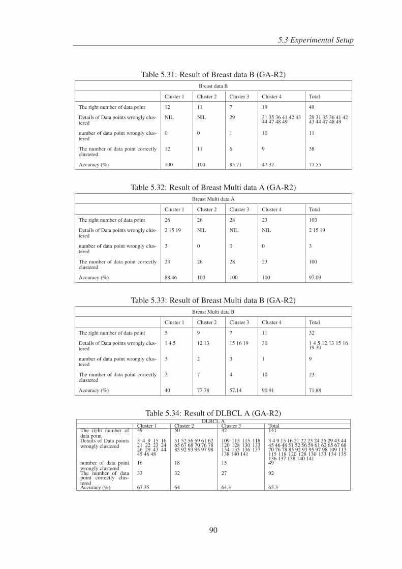
5.3 Experimental Setup
Table 5.31: Result of Breast data B (GA-R2)Breast data B
Cluster 1 Cluster 2 Cluster 3 Cluster 4 Total
The right number of data point 12 11 7 19 49
Details of Data points wrongly clus-tered
NIL NIL 29 31 35 36 41 42 4344 47 48 49
29 31 35 36 41 4243 44 47 48 49
number of data point wrongly clus-tered
0 0 1 10 11
The number of data point correctlyclustered
12 11 6 9 38
Accuracy (%) 100 100 85.71 47.37 77.55
Table 5.32: Result of Breast Multi data A (GA-R2)Breast Multi data A
Cluster 1 Cluster 2 Cluster 3 Cluster 4 Total
The right number of data point 26 26 28 23 103
Details of Data points wrongly clus-tered
2 15 19 NIL NIL NIL 2 15 19
number of data point wrongly clus-tered
3 0 0 0 3
The number of data point correctlyclustered
23 26 28 23 100
Accuracy (%) 88.46 100 100 100 97.09
Table 5.33: Result of Breast Multi data B (GA-R2)Breast Multi data B
Cluster 1 Cluster 2 Cluster 3 Cluster 4 Total
The right number of data point 5 9 7 11 32
Details of Data points wrongly clus-tered
1 4 5 12 13 15 16 19 30 1 4 5 12 13 15 1619 30
number of data point wrongly clus-tered
3 2 3 1 9
The number of data point correctlyclustered
2 7 4 10 23
Accuracy (%) 40 77.78 57.14 90.91 71.88
Table 5.34: Result of DLBCL A (GA-R2)DLBCL A
Cluster 1 Cluster 2 Cluster 3 TotalThe right number ofdata point
49 50 42 141
Details of Data pointswrongly clustered
3 4 9 15 1621 22 23 2426 29 43 4445 46 48
51 52 56 59 61 6265 67 68 70 76 7885 92 93 95 97 98
109 113 115 118120 128 130 133134 135 136 137138 140 141
3 4 9 15 16 21 22 23 24 26 29 43 4445 46 48 51 52 56 59 61 62 65 67 6870 76 78 85 92 93 95 97 98 109 113115 118 120 128 130 133 134 135136 137 138 140 141
number of data pointwrongly clustered
16 18 15 49
The number of datapoint correctly clus-tered
33 32 27 92
Accuracy (%) 67.35 64 64.3 65.3
90

5.3 Experimental Setup
Table 5.35: Result of DLBCL B (GA-R2)DLBCL B
Cluster 1 Cluster 2 Cluster 3 TotalThe right number ofdata point
42 51 87 180
Details of Data pointswrongly clustered
2 3 5 14 15 16 3234 35 36 37 39 4041
46 47 49 51 58 6577 79 92
96 97 103 119121 122 124 164167 179
2 3 5 14 15 16 32 34 35 36 3739 40 41 46 47 49 51 58 65 7779 92 96 97 103 119 121 122124 164 167 179
number of data pointwrongly clustered
14 9 10 33
The number of datapoint correctly clus-tered
28 42 77 147
Accuracy (%) 66.67 82.35 88.51 81.67
Table 5.36: Result of DLBCL C (GA-R2)DLBCL C
Cluster 1 Cluster 2 Cluster 3 Cluster 4 TotalThe right number ofdata point
17 16 13 12 58
Details of Data pointswrongly clustered
1 9 12 NIL 35 38 40 4142 43 45
48 52 53 54 55 56 5758
1 9 12 35 38 40 41 4243 45 48 52 53 54 5556 57 58
number of data pointwrongly clustered
3 0 7 8 18
The number of datapoint correctly clus-tered
14 16 6 4 40
Accuracy (%) 82.35 100 46.15 33.33 68.97
Table 5.37: Result of DLBCL D (GA-R2)DLBCL D
Cluster 1 Cluster 2 Cluster 3 Cluster4 TotalThe right number ofdata point
19 37 24 49 129
Details of Data pointswrongly clustered
1 17 20 28 32 43 4548 51 56
63 81 82 83 84 85 86 8788 89 90 91 92 93 9495 96 97 98 100 104105 108 112 114 117
1 17 20 28 32 43 45 4851 56 63 81 82 83 84 8586 87 88 89 90 91 92 9394 95 96 97 98 100 104105 108 112 114 117
number of data pointwrongly clustered
2 8 1 25 36
The number of datapoint correctly clus-tered
17 29 23 24 93
Accuracy (%) 89.47 78.38 95.83 48.98 72.09
Table 5.38: Result of Lung Cancer (GA-R2)Lung Cancer
Cluster 1 Cluster 2 Cluster 3 Cluster4 Total
The right number ofdata point
139 17 21 20 197
Details of Data pointswrongly clustered
15 24 26 68 71 78 79 8689 90 92 93 97 104 105109 111 112 114 117126 135 137 139
144 157 162167 168169 174
196 15 24 26 68 71 78 79 8689 90 92 93 97 104 105109 111 112 114 117126 135 137 139 144157 162 167 168 169174 196
number of data pointwrongly clustered
24 1 6 1 32
The number of datapoint correctly clus-tered
115 16 15 19 165
Accuracy (%) 82.73 94.12 71.43 95 83.76
91

5.3 Experimental Setup
Table 5.39: Result of Leukemia (GA-R2)Leukemia
Cluster 1 Cluster 2 TotalThe right number of data point 47 25 72Details of Data points wronglyclustered
6 7 8 22 23 28 31 32 33 34 3536 39 40 41 42 45
48 52 53 54 69 6 7 8 22 23 28 31 32 33 34 3536 39 40 41 42 45 48 52 53 5469
number of data point wronglyclustered
17 5 22
The number of data point cor-rectly clustered
30 20 50
Accuracy (%) 63.83 80 69.44
Table 5.40: Result of St. Jude Leukemia (GA-R2)St. Jude Leukemia
Cluster 1 Cluster 2 Cluster 3 Cluster 4 Cluster 5 Cluster 6 TotalThe right numberof data point
15 27 64 20 43 79 248
Details of Datapoints wronglyclustered
2 NIL 61 69 7199
109 110111 112
131 144157 168
NIL 2 61 69 71 99 109110 111 112 131144 157 168
number of datapoint wronglyclustered
1 0 4 4 4 0 13
The number ofdata point cor-rectly clustered
13 27 60 16 39 79 234
Accuracy (%) 86.67 100 93.75 80 90.7 100 94.35
Table 5.41: Result of Cho Data (GA-R2)Cho Data
Cluster 1 Cluster 2 Cluster 3 Cluster4 Cluster5 TotalTherightnumberof datapoint
67 135 75 54 55 386
Detailsof Datapointswronglyclustered
2 6 25 2628 32 4345 56 6466
82 90 96110 112125 127128 129130 133134 137146 173176 178180 181187 188189 190191 199
203 205 207 210 212215 217 218 220 221222 225 226 227 228229 231 236 237 238239 241 243 246 247248 249 250 251 254255 256 257 258 259260 261 262 263 268269 270 272 273 276277
291293294296297299321322324
332342347354359361366370
2 6 25 26 28 32 43 45 56 64 66 82 9096 110 112 125 127 128 129 130 133134 137 146 173 176 178 180 181 187188 189 190 191 199 203 205 207 210212 215 217 218 220 221 222 225 226227 228 229 231 236 237 238 239 241243 246 247 248 249 250 251 254 255256 257 258 259 260 261 262 263 268269 270 272 273 276 277 291 293 294296 297 299 321 322 324 332 342 347354 359 361 366 370
numberof datapointwronglyclustered
11 25 46 9 8 99
Thenumberof datapointcorrectlyclustered
56 110 29 45 47 287
Accuracy(%)
83.58 81.48 38.67 83.33 85.45 74.35
92

5.3 Experimental Setup
Table 5.42: Result of Iyer Data (GA-R2)IyerData
Therightnum-ber ofdatapoint
Details of Data points wrongly clustered numberof datapointwronglyclus-tered
Thenum-ber ofdatapointcor-rectlyclus-tered
Accuracy(%)
Cluster 1 33 1 2 3 4 5 6 7 8 9 10 11 12 13 14 15 16 17 18 19 21 22 23 28 29 30 31 26 7 21.21Cluster 2 100 NIL 0 100 100Cluster 3 145 143 146 157 161 162 163 164 166 167 168 169 170 171 172 173 174
175 176 177 178 179 180 181 186 187 188 190 191 192 193 194 197198 199 200 201 202 203 204 206 210 211 213 224 225 226 231 243244 245 248 249 255 265 267 270 271 273 274 275 278
61 84 57.93
Cluster 4 34 280 283 284 285 286 287 294 295 296 297 298 299 300 301 303 15 19 55.82Cluster 5 43 313 314 315 316 317 318 319 320 321 322 324 325 326 327 328 329
330 331 332 333 334 335 342 343 348 349 352 35528 15 34.89
Cluster 6 7 359 1 6 85.71Cluster 7 34 365 366 367 370 373 378 379 381 383 384 387 388 389 390 391 392
39317 17 50
Cluster 8 14 399 401 2 12 85.71Cluster 9 63 411 412 413 414 415 416 417 418 419 420 421 422 423 424 425 426
427 428 429 430 431 432 433 434 436 437 438 439 440 442 443 444445 446 447 448 449 450 451 452 453 454 455 456 457 458 459 460461 462 463 464 465 466 467 468 469 470 473
59 4 6.35
Cluster10
19 474 475 476 477 478 479 480 481 482 483 484 485 486 487 488 489490 492
18 1 5.26
Cluster11
25 493 494 495 496 497 498 499 500 502 503 504 505 506 507 508 509510 511 512 513 514 515 516 517
24 1 4
Total 517 1 2 3 4 5 6 7 8 9 10 11 12 13 14 15 16 17 18 19 21 22 23 28 29 30 31 143146 157 161 162 163 164 166 167 168 169 170 171 172 173 174 175176 177 178 179 180 181 186 187 188 190 191 192 193 194 197 198199 200 201 202 203 204 206 210 211 213 224 225 226 231 243 244245 248 249 255 265 267 270 271 273 274 275 278 280 283 284 285286 287 294 295 296 297 298 299 300 301 303 313 314 315 316 317318 319 320 321 322 324 325 326 327 328 329 330 331 332 333 334335 342 343 348 349 352 355 359 365 366 367 370 373 378 379 381383 384 387 388 389 390 391 392 393 399 401 411 412 413 414 415416 417 418 419 420 421 422 423 424 425 426 427 428 429 430 431432 433 434 436 437 438 439 440 442 443 444 445 446 447 448 449450 451 452 453 454 455 456 457 458 459 460 461 462 463 464 465466 467 468 469 470 473 474 475 476 477 478 479 480 481 482 483484 485 486 487 488 489 490 492 493 494 495 496 497 498 499 500502 503 504 505 506 507 508 509 510 511 512 513 514 515 516 517
251 266 51.45
Table 5.43 to Table 5.55 shows the result obtained by GA-R3 for bioinformatics data.
All these table contains the following information of GA-R3 for bioinformatics data:
The right number of data point in each cluster, details of data point wrongly clustered
in each cluster, number of data points in each cluster, number of data point correctly
clustered in each cluster and individual accuracy of each cluster in a data as well as
overall accuracy for each bioinformatics data.
Table 5.43 contains the result obtained by GA-R3 for Breast Data A. Number of data
point wrongly clustered in cluster 1 is five, in cluster 2 is six and in cluster 3 is three. The
total number of data points wrongly clustered is 14. Details of the data point wrongly
clustered are {5 6 7 8 11 20 31 38 39 46 56 66 80 81}. The overall accuracy obtained
for Breast Data A using GA-R3 was 85.71 % .
Table 5.44 contains the result obtained by GA-R3 for Breast Data B. Details of the data
point wrongly clustered are {17 28 31 35 36 41 42 47 48 49}. Notably cluster 1 achieves
93

5.3 Experimental Setup
accuracy 100 %. The overall accuracy obtained for Breast Data B using GA-R3 was
79.59 % .
Table 5.45 contains the result obtained by GA-R3 for Breast Multi Data A. Details of
the data point wrongly clustered are {2 15 19 25 26 38 60 70}. The overall accuracy
obtained for Breast Multi Data A using GA-R3 was 92.23 % .
Table 5.46 contains the result obtained by GA-R3 for Breast Multi Data B. The total
number of data points wrongly clustered is 17. The overall accuracy obtained for Breast
Multi Data B using GA-R3 was 53.125 % .
Table 5.47 contains the result obtained by GA-R3 for DLBCL A. The total number of
data points wrongly clustered is 33. The overall accuracy obtained for DLBCL A using
GA-R3 was 76.6 %.
Table 5.48 contains the result obtained by GA-R3 for DLBCL B. The total number of
data points wrongly clustered is 38. The overall accuracy obtained for DLBCL B using
GA-R3 was 78.89 % .
Table 5.49 contains the result obtained by GA-R3 for DLBCL C. The total number of
data points wrongly clustered is 9. The overall accuracy obtained for DLBCL C using
GA-R3 was 84.48 % .
Table 5.50 contains the result obtained by GA-R3 for DLBCL D The total number of
data points wrongly clustered is 49. The overall accuracy obtained for DLBCL D using
GA-R3 was 62.01 % .
Table 5.51 contains the result obtained by GA-R3 for Lung Cancer. The total number
of data points wrongly clustered is 41. The overall accuracy obtained for Lung Cancer
using GA-R3 was 79.2 %.
Table 5.52 contains the result obtained by GA-R3 for Leukemia Cancer. The total num-
ber of data points wrongly clustered is 32. The overall accuracy obtained for Leukemia
Cancer using GA-R3 was 55.56%.
Table 5.53 contains the result obtained by GA-R3 for St. Jude Leukemia Cancer. The
total number of data points wrongly clustered is 29. Notably cluster 2 and cluster 6
achieves accuracy 100%. The overall accuracy obtained for St. jude Leukemia Cancer
using GA-R3 was 88.31 %.
94

5.3 Experimental Setup
Table 5.54 contains the result obtained by GA-R3 for Cho data. The total number of
data points wrongly clustered is 133. The overall accuracy obtained for Cho data using
GA-R3 was 65.54 %.
Table 5.55 contains the result obtained by GA-R3 for Iyer data. The total number of
data points wrongly clustered is 248. The overall accuracy obtained for Iyer data using
GA-R3 was 52.03 %.
Table 5.43: Result of Breast data A (GA-R3)Breast data A
Cluster 1 Cluster 2 Cluster 3 Total
The right number of data point 11 51 36 98
Details of Data points wrongly clustered 5 6 7 8 11 20 31 38 39 46 56 66 80 81 5 6 7 8 11 20 31 38 3946 56 66 80 81
number of data point wrongly clustered 5 6 3 14
The number of data point correctly clus-tered
6 45 33 84
Accuracy (%) 54.55 88.24 91.67 85.71
Table 5.44: Result of Breast data B (GA-R3)Breast data B
Cluster 1 Cluster 2 Cluster 3 Cluster 4 Total
The right number of datapoint
12 11 7 19 49
Details of Data pointswrongly clustered
NIL 17 28 31 35 36 41 42 47 4849
17 28 31 35 36 41 4247 48 49
number of data point wronglyclustered
0 1 1 8 10
The number of data point cor-rectly clustered
12 10 6 11 39
Accuracy (%) 100 90.91 85.71 57.89 79.59
95

5.3 Experimental Setup
Table 5.45: Result of Breast Multi data A (GA-R3)Multi Breast data A
Cluster 1 Cluster 2 Cluster 3 Cluster 4 Total
The right number of datapoint
26 26 28 23 103
Details of Data pointswrongly clustered
2 15 19 2526
38 60 70 NIL 2 15 19 25 26 38 60 70
number of data point wronglyclustered
5 1 2 0 8
The number of data point cor-rectly clustered
21 25 26 23 95
Accuracy (%) 80.76 96.15 92.86 100 92.23
Table 5.46: Result of Breast Multi data B (GA-R3)Multi Breast data B
Cluster 1 Cluster 2 Cluster 3 Cluster 4 Total
The right number of datapoint
5 9 7 11 32
Details of Data pointswrongly clustered
1 4 5 12 13 16 19 22 23 26 28 29 30 3132
1 4 5 12 13 16 19 2223 26 28 29 30 31 32
number of data point wronglyclustered
3 2 2 8 15
The number of data point cor-rectly clustered
2 7 5 3 17
Accuracy (%) 40 77.78 71.43 27.27 53.125
Table 5.47: Result of DLBCL A (GA-R3)DLBCL A
Cluster 1 Cluster 2 Cluster 3 Total
The right number ofdata point
49 50 42 141
Details of Data pointswrongly clustered
3 4 9 15 1622 24 29 4344 45 46 48
51 62 76 7893 95 97 98
113 115 118 120 128 130134 136 137 138 140 141 34 9 15 16 22 24 29 43 4445 46 48 51 62 76 78 9
3 95 97 98 113 115 118 120 128130 134 136 137 138 140 141
number of data pointwrongly clustered
13 8 12 33
The number of datapoint correctly clus-tered
36 42 30 108
Accuracy (%) 73.47 84 71.43 76.6
96

5.3 Experimental Setup
Table 5.48: Result of DLBCL B (GA-R3)DLBCL B
Cluster 1 Cluster 2 Cluster 3 Total
The right numberof data point
42 51 87 180
Details of Datapoints wronglyclustered
2 3 5 14 15 16 3234 35 36 37 39 4041
43 46 47 49 5153 58 60 62 6465 77 79 92
96 97 103 119121 122 124164 167 179
2 3 5 14 15 16 32 34 35 36 37 39 40 41 43 4647 49 51 53 58 60 62 64 65 77 79 92 96 97103 119 121 122 124 164 167 179
number of datapoint wronglyclustered
14 14 10 38
The number ofdata point cor-rectly clustered
28 37 77 142
Accuracy (%) 66.67 72.55 88.51 78.89
Table 5.49: Result of DLBCL C (GA-R3)DLBCL C
Cluster 1 Cluster 2 Cluster 3 Cluster4 Total
The right number of datapoint
17 16 13 12 58
Details of Data pointswrongly clustered
12 NIL 35 38 40 41 42 43 45 47 12 35 38 40 41 42 4345 47
number of data pointwrongly clustered
1 0 7 1 9
The number of data pointcorrectly clustered
16 16 6 11 49
Accuracy (%) 94.11 100 46.15 91.67 84.48
Table 5.50: Result of DLBCL D (GA-R3)DLBCL D
Cluster 1 Cluster 2 Cluster 3 Cluster4 TotalThe right numberof data point
19 37 24 49 129
Details of Datapoints wronglyclustered
1 7 9 13 1417 19
20 28 3032 40 4142 43 4548 51 56
63 64 6566 68
81 82 83 84 85 86 8788 89 90 91 92 93 9495 96 97 98 100 104105 108 112 114 117
1 7 9 13 14 17 19 20 28 30 32 4041 42 43 45 48 51 56 63 64 6566 68 81 82 83 84 85 86 87 8889 90 91 92 93 94 95 96 97 98100 104 105 108 112 114 117
number of datapoint wronglyclustered
7 12 5 25 49
The number ofdata point cor-rectly clustered
12 25 19 24 80
Accuracy (%) 63.16 67.57 79.17 48.98 62.01
97

5.3 Experimental Setup
Table 5.51: Result of Lung Cancer (GA-R3)Lung Cancer
Cluster 1 Cluster 2 Cluster 3 Cluster4 TotalThe right number ofdata point
139 17 21 20 197
Details of Datapoints wronglyclustered
15 18 19 20 21 24 2633 42 50 68 69 71 7678 79 86 89 90 92 9397 104 105 109 111112 114 117 126 135137 139
144 157 162167 168169 174
196 15 18 19 20 21 24 26 33 4250 68 69 71 76 78 79 86 8990 92 93 97 104 105 109 111112 114 117 126 135 137 139144 157 162 167 168 169 174196
number of datapoint wronglyclustered
33 1 6 1 41
The number of datapoint correctly clus-tered
106 16 15 19 156
Accuracy (%) 76.26 94.11 71.43 95 79.2
Table 5.52: Result of Leukemia (GA-R3)Leukemia
Cluster 1 Cluster 2 TotalThe right number of data point 47 25 72Details of Data points wrongly clus-tered
6 7 8 19 22 23 28 3132 33 34 35 36 39 4041 42 45
48 50 51 52 53 5455 56 57 58 59 6169 71
6 7 8 19 22 23 28 31 32 33 34 35 3639 40 41 42 45 48 50 51 52 53 54 5556 57 58 59 61 69 71
number of data point wrongly clus-tered
18 14 32
The number of data point correctlyclustered
29 11 40
Accuracy (%) 61.70 44 55.56
Table 5.53: Result of St. Jude Leukemia (GA-R3)St. Jude Leukemia
Cluster 1 Cluster 2 Cluster 3 Cluster4 Cluster5 Cluster6 TotalThe right num-ber of datapoint
15 27 64 20 43 79 248
Details of Datapoints wronglyclustered
2 NIL 43 48 4950 58 6162 69 7172 74 7686 91 9396 97 99102 103
109 110111 112
127 131157 168
NIL 2 43 48 49 5058 61 62 69 7172 74 76 86 9193 96 97 99102 103 109110 111 112127 131 157168
number of datapoint wronglyclustered
1 0 20 4 4 0 29
The number ofdata point cor-rectly clustered
14 27 44 16 39 79 219
Accuracy (%) 93.33 100 68.75 80 90.7 100 88.31
98

5.3 Experimental Setup
Table 5.54: Result of Cho Data (GA-R3)Cho Data
Cluster1
Cluster 2 Cluster 3 Cluster4 Cluster5 Total
The rightnumber ofdata point
67 135 75 54 55 386
Detailsof Datapointswronglyclustered
2 6 2526 2829 3243 4556 6466
82 90 96110 112125 127128 129130 133134 137146 173176 178180 181187 188189 190191 199
203 205 206207 210 212213 214 215217 218 219220 221 222225 226 227228 229 231236 237 238239 241 243246 247 248249 250 251254 255 256257 258 259260 261 262263 268 269270 272 273276 277
278 279 281282 285 286287 289 290291 292 293294 295 296297 298 299300 301 302303 304 305306 307 308309 310 311312 314 315316 317 318321 322 324325 326
332342347354359361366370
2 6 25 26 28 29 32 43 45 56 64 66 82 90 96110 112 125 127 128 129 130 133 134 137146 173 176 178 180 181 187 188 189 190191 199 203 205 206 207 210 212 213 214215 217 218 219 220 221 222 225 226 227228 229 231 236 237 238 239 241 243 246247 248 249 250 251 254 255 256 257 258259 260 261 262 263 268 269 270 272 273276 277 278 279 281 282 285 286 287 289290 291 292 293 294 295 296 297 298 299300 301 302 303 304 305 306 307 308 309310 311 312 314 315 316 317 318 321 322324 325 326 332 342 347 354 359 361 366370
number ofdata pointwronglyclustered
9 25 50 41 8 133
The num-ber of datapoint cor-rectly clus-tered
58 110 25 13 47 253
Accuracy(%)
86.57 81.481 33.33 31.71 87.04 65.544
Table 5.55: Result of Iyer Data (GA-R3)Iyer Data
Therightnumberof datapoint
Details of Data points wrongly clustered Number ofdata pointwronglyclustered
Thenumberof datapointcorrectlyclustered
Accuracy(%)
Cluster1 33 1 2 3 4 5 6 7 8 9 10 11 12 13 14 15 16 17 18 19 21 22 23 28 29 3031
26 7 78.79
Cluster2 100 NIL 0 100 100Cluster3 145 143 146 157 161 162 163 164 166 167 168 169 170 171 172 173
174 175 176 177 178 179 180 181 186 187 188 190 191 192 193194 197 198 199 200 201 202 203 204 206 210 211 213 224 225226 231 243 244 245 248 249 255 265 267 270 271 273 274 275278
61 84 57.93
Cluster4 34 280 283 284 285 286 287 294 295 296 297 298 299 300 301 303 15 19 55.88Cluster5 43 313 314 315 316 317 318 319 320 321 322 324 325 326 327 328
329 330 331 332 333 334 335 342 343 348 349 352 35528 15 34.89
Cluster6 7 359 1 6 85.71Cluster7 34 365 366 367 370 373 378 379 381 383 384 387 388 389 390 391
392 39317 17 50
Cluster8 14 399 401 2 12 85.71Cluster9 63 411 412 413 414 415 416 417 418 419 420 421 422 423 424 426
427 428 429 430 431 432 433 434 436 437 438 439 440 442 443444 445 447 448 449 450 451 452 453 454 455 456 457 458 459460 461 462 463 464 465 466 467 468 469 473
56 7 11.11
Cluster10 19 474 475 476 477 478 479 480 481 482 483 484 485 486 487 488489 490 492
18 1 5.26
Cluster11 25 493 494 495 496 497 498 499 500 502 503 504 505 506 507 508509 510 511 512 513 514 515 516 517
24 1 4
Total 517 1 2 3 4 5 6 7 8 9 10 11 12 13 14 15 16 17 18 19 21 22 23 28 29 3031 143 146 157 161 162 163 164 166 167 168 169 170 171 172173 174 175 176 177 178 179 180 181 186 187 188 190 191 192193 194 197 198 199 200 201 202 203 204 206 210 211 213 224225 226 231 243 244 245 248 249 255 265 267 270 271 273 274275 278 280 283 284 285 286 287 294 295 296 297 298 299 300301 303 313 314 315 316 317 318 319 320 321 322 324 325 326327 328 329 330 331 332 333 334 335 342 343 348 349 352 355359 365 366 367 370 373 378 379 381 383 384 387 388 389 390391 392 393 399 401 411 412 413 414 415 416 417 418 419 420421 422 423 424 426 427 428 429 430 431 432 433 434 436 437438 439 440 442 443 444 445 447 448 449 450 451 452 453 454455 456 457 458 459 460 461 462 463 464 465 466 467 468 469473 474 475 476 477 478 479 480 481 482 483 484 485 486 487488 489 490 492 493 494 495 496 497 498 499 500 502 503 504505 506 507 508 509 510 511 512 513 514 515 516 517
248 269 52.03
99

5.3 Experimental Setup
Final fitness value after convergence of GA-R1, GA-R2 and GA-R3 based clustering
algorithms has been tabulated in Table 5.56. GA-R1 attains minimum fitness value in
case of Iyer, Breast data B and Breast Multi data A. GA-R2 attains minimum fitness
value in case of Leukemia, Breast Multi Data B, DLBCL C, DLBCL D and Lung Can-
cer. GA-R3 attains minimum fitness value in case of Cho Data, Breast Data A, DLBCL
A, DLBCL B and St. jude Leukemia data. It may be noted that GA-R2 and GA-R3
attains same fitness value for Iyer data (i.e., 48.3397) but minimum fitness value was
attained by GA-R1 (i.e., 47.6926). GA-R1 and GA-R2 attains minimum fitness value
for Breast Data B and it is optimal compared to GA-R3. Also, GA-R1 and GA-R2
attains same minimum fitness value for Breast Multi Data A and it is optimal compared
to GA-R3.
Table 5.56: Final Fitness Function value for Bioinformatics DataDatasetSl.No.
Datasets GA-R1 GA-R2 GA-R3
3 Iyer data/Serum data 0.02096 0.02068 0.02068
4 Cho data (yeast data) 0.02146 0.02157 0.02397
5 Leukemia (Golub Exper-iment)
0.10374 0.12475 0.10965
6 Breast data A 0.11518 0.10594 0.11548
7 Breast data B 0.33563 0.33563 0.33242
8 Breast Multi data A 0.09014 0.09014 0.0895
9 Breast Multi data B 0.18350 0.23075 0.2247
10 DLBCL A 0.06406 0.06410 0.06841
11 DLBCL B 0.06150 0.06207 0.06311
12 DLBCL C 0.18437 0.19119 0.18194
13 DLBCL D 0.14457 0.15479 0.1426
14 Lung Cancer 0.03538 0.03675 0.03538
15 St. Jude Leukemia data 0.04475 0.04454 0.04512
Table 5.57 summarizes the accuracy of GA based clustering algorithm for bioinformat-
ics data. Average, best and worst case analysis has been carried out on bioinformatics
data for GA-R1, GA-R2 and GA-R3. As far as best case analysis is concerned, GA-R1
performs better in case of Iyer data, Breast multi data A, DLBCL B data ; GA-R3 per-
forms better in case of Iris, Breast data B, DLBCL A, DLBCL C and in rest of cases
GA-R2 performs better compared to GA-R1 and GA-R3 (Table 5.57 ).
100

5.4 Comparative Studies on HCM, SCM and GA based Clustering Algorithm
Table 5.57: Comparison of GA based clustering algorithm for Bioinformatics data usingAccuracy
DatasetSl.No.
Datasets # Sam-ples/genes
GA-R1 GA-R2 GA-R3
#cor-rect
Accuracy(%) #cor-rect
Accuracy(%) #cor-rect
Accuracy(%)
3 Iyer data/Serum data 517 269 52.0309 266 51.4507 266 51.45074 Cho data (yeast data) 386 259 67.0984 287 74.3523 250 64.76685 Leukemia (Golub Experi-
ment)72 40 55.566 50 69.4444 40 55.566
6 Breast data A 98 88 89.7959 91 92.8571 84 85.71437 Breast data B 49 38 77.5510 38 77.5510 39 79.59188 Breast Multi data A 103 100 97.0874 100 97.0874 95 92.23309 Breast Multi data B 32 20 62.5000 23 71.8750 17 53.125010 DLBCL A 141 98 69.5035 92 65.2482 108 76.595711 DLBCL B 180 152 84.4444 147 81.6667 142 78.888912 DLBCL C 58 46 79.3103 40 68.9655 50 86.206913 DLBCL D 129 85 65.8915 93 72.0930 80 62.015514 Lung Cancer 197 156 79.1878 165 83.7563 156 79.187815 St. Jude Leukemia data 248 233 93.9516 235 94.7581 219 88.3065
5.4 Comparative Studies on HCM, SCM and GA basedClustering Algorithm
To evaluate performance of HCM, SCM and GA based clustering algorithm; Clustering
Accuracy was used as cluster validation metric. Extensive computer simulation ( Table
5.57) shows that GA based clustering algorithm was able to provide the highest accu-
racy and generalization results compared to Non-GA based clustering Algorithm in all
cases. Average, best and worst case analysis have been also carried out on machine
learning data as well as bioinformatics data. Soft C-means shows superior performance
in 11 cases (Iris, WBCD, Cho/yeast data, Breast data A, Breast data B, Breast Multi
data A, DLBCL A, , DLBCL C, DLBCL D, Lung Cancer, St. Jude Leukemia data)
over Hard C-means algorithm; while Hard C-mean shows superior performance in 4
cases (Iyer/serum, Leukemia, Breast Multi data B, DLBCL B) over Soft C-means (Ta-
ble 5.58).
GA based clustering algorithm always shows superior performance compared to Non-
GA based clustering algorithm. As far as best case analysis is concerned, GA-R1 per-
forms better in case of Iyer data, Breast multi data A, DLBCL B data ; GA-R3 performs
better in case of Iris, Breast data B, DLBCL A, DLBCL C and in rest of cases GA-R2
performs better compared to GA-R1 and GA-R3 (Table 5.58 ).
101

5.5 Conclusion
Table 5.58: Comparison of HCM, SCM and GA based clustering algorithm for allfifteen data using Accuracy
Sl.No.
Datasets #Sam-ples
Hard C-means Soft C-means GA-R1 GA-R2 GA-R3
#cor-rect
Accuracy(%)
#cor-rect
Accuracy(%)
#cor-rect
Accuracy(%)
#cor-rect
Accuracy(%)
#cor-rect
Accuracy(%)
1 Iris 150 133 88.67 136 90.67 140 93.33 144 96 150 1002 WBCD 683 654 95.75 656 96.05 657 96.1933 661 96.7789 665 97.36463 Iyer
data/Serumdata
517 268 51.84 252 48.74 269 52.0309 266 51.4507 266 51.4507
4 Cho data(yeast data)
386 235 60.88 246 63.73 259 67.0984 287 74.3523 250 64.7668
5 Leukemia(GolubExperiment)
72 43 59.72 40 55.56 40 55.566 50 69.4444 40 55.566
6 Breast data A 98 71 72.44 86 87.75 88 89.7959 91 92.8571 84 85.71437 Breast data B 49 26 53.06 32 65.30 38 77.5510 38 77.5510 39 79.59188 Breast Multi
data A103 82 79.61 93 90.29 100 97.0874 100 97.0874 95 92.2330
9 Breast Multidata B
32 17 53.125 16 50 20 62.5000 23 71.8750 17 53.1250
10 DLBCL A 141 75 53.191 83 58.86 98 69.5035 92 65.2482 108 76.595711 DLBCL B 180 140 77.78 136 75.56 152 84.4444 147 81.6667 142 78.888912 DLBCL C 58 30 51.7241 44 75.86 46 79.3103 40 68.9655 50 86.206913 DLBCL D 129 55 42.64 65 50.38 85 65.8915 93 72.0930 80 62.015514 Lung Cancer 197 142 72.0812 150 76.14 156 79.1878 165 83.7563 156 79.187815 St. Jude
Leukemiadata
248 211 85.08 219 88.31 233 93.9516 235 94.7581 219 88.3065
5.5 Conclusion
In this chapter, four different types of encoding schemes for chromosome have been
studied for clustering. GA based clustering algorithm overcomes the limitation of HCM
and SCM clustering algorithm (i.e., to get trapped in local optimum solution). Extensive
computer simulation shows that GA based clustering algorithm was able to provide
the highest accuracy and generalization results compared to Non-GA based clustering
algorithm (HCM and SCM) in all fifteen cases.
As far as best case analysis is concerned, GA-R1 performs better in case of Iyer data,
Breast multi data A, DLBCL B data; GA-R3 performs better in case of Iris, Breast data
B, DLBCL A, DLBCL C and in rest of cases GA-R2 performs better compared to GA-
R1 and GA-R3.
As far as memory utilization is concerned, it is advisable to go for GA-R2 clustering
algorithm when number of features are less in number in a dataset otherwise to go for
GA-R1 clustering algorithm.
102

Chapter 6
Brute Force based Clustering AndSimulated Annealing basedPreprocessing of Data
This chapter is broadly divided into two section:
• An incremental Brute-Force approach for Clustering and
• Preprocessing (diversification) of data using Simulated Annealing (SA).
6.1 An Incremental Brute-Force Approach for Cluster-ing
The Brute-Force approach for clustering was intended for three specific purposes. These
are as follows:
• It should not require information like no. of clusters from user i.e it should help
in automatic evolution of clusters.
• It should be computationally faster so that it may be useful for high dimensional
data.
• It should be efficient in nature in terms of cluster formation.
The main steps involved in the proposed approach are shown in fig. 6.1.
Algorithmic Steps of An incremental Brute-Force Approach for Clustering:
Given a piece of gene expression data: the first step is Data preprocessing. In general,
it can be done by simple transformation or normalization performed on single variables,
filters and calculation of new variables from existing ones. In proposed work, only the
103

6.1 An Incremental Brute-Force Approach for Clustering
Figure 6.1: Flow-Chart of Brute-Force Approach based Clustering Algorithm
first of these is implemented. Scaling of variables is of special importance, say for
example, Euclidean metric has been used to measure distances between vectors. If
one variable has values in the range of 0,...,1000 and another in the range of 0,...,1
the former will almost completely dominate the cluster formation because of its greater
impact on the distances measured. Typically, one would want the variables to be equally
important. The standard way to achieve this is to linearly scale all variables so that their
variances are equal to one [93].
Second step, is to compute Distance matrix ‘D’ from processed data obtained in step
first. ‘Di j’ represents the distance between the expression patterns for genes ‘i’ and ‘ j’.
Although a number of alternative measures could be used to calculate the similarity
between gene expressions, Euclidean distance metric [7], [8], [9], [10] has been used
due to its wide application range.
In the Third step, a threshold value, called ‘θ ’, is computed as follows:
‘θ = z × Average distance between genes’, where ’z’ is a positive constant. The value
of ‘z’ is chosen in such a way that number of clusters lies between 2 to√
n. Lesser the
value of ‘z’, more the number of clusters. ‘θ ’ is calculated based on distance matrix,
that generates no. of cluster automatically. This threshold value is computed dynam-
104

6.1 An Incremental Brute-Force Approach for Clustering
ically and changes after each cluster formation. This depends on two factor, first, the
average similarity of whole gene and secondly, how many genes are left for next cluster
formation.
Fourth step is an iterative step. If distance between two genes are less than threshold
value ‘θ ’, it forms a first cluster otherwise it falls under second cluster . This step is
repeated iteratively unless all the genes fall under some particular clusters.
In the final step, a validation test is performed to evaluate the quality of the clustering
result produced in step fourth.
6.1.1 Experimental Evaluation
This section describes about the experimental setup and datasets used for carrying the
simulation performance of an incremental Brute-Force approach for clustering.
1. Experimental Setup
To validate the feasibility and performance of the proposed approach, implemen-
tation has been done in MATLAB 7.0 (C2D, 2.0 GHz, 2 GB RAM) and applied
it to both of real gene expression data and synthetic data.
2. Datasets
To evaluate the performance of proposed approach, two real and one synthetic
gene expression data has been considered for study. These datasets do not possess
referenced (class-labeled) information available to the data.
• Datasets I is a synthetic data of [10x3] matrix.
• Datasets II represents Wisconsin breast cancer dataset and is obtained from
the University Medical Centre, Institute of Oncology, Ljubljana, Yugoslavia
(http://mlearn.ics.uci.edu or
ftp://ftp.ics.uci.edu/pub/machine-learning-databases/breast- cancer-wisconsin).
The dataset contains 699 instances and each instances are having 9 features.
There are 16 datapoints with missing values. Missing values have been re-
placed by mean of the feature of column in which missing value was found.
105

6.1 An Incremental Brute-Force Approach for Clustering
• Datasets III is a real biological microarray data of [118x60] matrix that
represents growth inhibition factors when 118 drugs with putatively under-
stood methods of action were applied to the NCI60 cell lines. The original
data can be downloaded from
http://discover.nci.nih.gov/nature2000/data/selected data/a matrix118.txt.
6.1.2 Cluster Validation Metrics
Since all the datasets (Datasets I, II and III) considered in this chapter for simulation
study do not possess class-labeled information, clustering accuracy can not be used
as a cluster validation metric. In this chapter of the thesis, HS Ratio [45], [20], [13]
is used as cluster validation metric to validate the quality of clusters. Details of the
HS Ratio has been already discussed in section 5.2.3. It may be noted that “the quality
of cluster V increases with higher homogeneity values within C and lower separation
values between V and other clusters”.
6.1.3 Results and Discussion
Brute-Force based clustering approach has been simulated for different value of ‘z’ and
result obtained were tabulated in Table 6.1. The value of parameter ‘z’ has been taken
in range {0.3,1.8} for simulation studies. The algorithm generates number of cluster
automatically. The quality of the clusters formed were assessed using HS Ratio.
The simulation results shown in Table 6.2 show that the proposed Brute-Force based
clustering approach may perform better compared to HCM clustering algorithm when
the no. of cluster is high.
Table 6.3 shows the proposed Brute Force based Clustering approach is computationally
quite faster than conventional HCM clustering algorithm(fig. 6.2) and thus it may be
very useful while dealing with high dimensional microarray data.
Another important feature of the proposed Brute-Force based clustering approach
in opposite to HCM clustering algorithm is that, unlike HCM Clustering algorithm it
does not require the value of number of cluster i.e., ‘C’ from user.
106

6.1 An Incremental Brute-Force Approach for Clustering
Table 6.1: HS Ratio value for Brute-Force approach based clusteringBrute-Force Approach based Clustering Algorithm
- TrialNo
z θ No ofcluster
Haverage Saverage HS Ratio
Sample data [10 X 3]
1 0.3000 2.383434e+000 5 0.1425 0.3047 0.4676
2 .7 7.944781e+000 3 0.2877 0.1119 2.5706
3 0.7000 5.561347e+000 4 0.2189 0.3073 0.7122
4 1.2000 9.533738e+000 2 0.5233 0.1569 3.3343
5 1.3 1.032822e+001 2 0.4649 0.8592 0.5411
6 1.4000 1.112269e+001 2 0.4649 0.8592 0.5411
Breast Cancer [699 X 9]
1 .9500 9.551604e+000 24 0.4889 0.5077 0.9630
2 1 1.005432e+001 20 0.5946 0.5644 1.0535
3 1.05 1.055704e+001 15 0.8097 0.5338 1.5168
4 1.1000 1.105975e+001 12 1.0299 0.6057 1.7003
5 1.2000 1.206518e+001 8 1.5935 0.6174 2.5808
6 1.4 1.407605e+001 4 3.2558 0.5732 5.6799
7 1.6000 1.608691e+001 3 4.5015 0.5290 7.9747
8 1.8000 1.809778e+001 2 6.8196 0.2794 24.4060
Cancer Data [118 X 60]
1 0.7000 1.146838e+001 9 0.5360 0.8097 0.6620
2 0.7300 1.195988e+001 8 0.6351 0.7892 0.8047
3 1 1.638340e+001 5 1.1719 0.8240 1.4221
4 1.1000 1.802174e+001 4 1.5445 0.5712 1.5592
5 1.6000 2.621344e+001 3 2.3853 0.4399 2.1310
Table 6.2: Comparative study on HCM and Brute Force approach based clusteringNo. Of Cluster HCM clustering algorithm Brute Force Approach
Sample data [10 X 3]
3 2.7195 2.5706
2 3.3343 0.5411
Breast Cancer [699 X 9]
20 0.4899 1.0535
15 0.5881 1.5168
12 1.0293 1.7003
8 1.9899 2.5808
4 6.3689 5.6799
3 8.5102 7.9747
2 38.1630 24.4060
Cancer Data [118 X 60]
9 0.5595 0.6620
8 0.5522 0.8047
5 1.0069 1.1043
4 2.7040 1.5592
3 5.4224 2.1310
107

6.1 An Incremental Brute-Force Approach for Clustering
Table 6.3: Computational time for HCM and Brute-Force based clustering AlgorithmDatasets Data Size HCM clustering Algo-
rithmBrute-Force based clus-tering
Sample data [10x3] Matrix 0.0203 Second 0.0008 Second
Breast Cancer [699x9] Matrix 0.5 Second 0.344 Second
Cancer Data [118x60] Matrix 0.047 Second 0.0310 Second
Figure 6.2: Comparison of Computational time for HCM and Brute-Force apraoachbased clustering
6.1.4 Conclusion
In this section of the thesis, a Brute-Force approach based clustering has been proposed.
Performance evaluation of proposed approach has been compared with conventional
HCM clustering Algorithm using artificial/synthetic and real datasets (machine learning
as well as bioinformatics data). Simulation results obtained shows that the proposed ap-
proach can achieve a high degree of automation and efficiency. The proposed approach
does not require the value of number of cluster ‘C’ from user. The proposed approach
is also quite faster than HCM clustering algorithm and thus it could be useful for high
dimensional microarray data. As far as efficiency is concerned, proposed Brute-Force
based clustering approach may perform better compared to HCM clustering algorithm
when the no. of clusters are higher in value.
108

6.2 Preprocessing of Data using Simulated Annealing
6.2 Preprocessing of Data using Simulated Annealing
Simulated Annealing (SA) exploits an analogy between the way in which a metal cools
and freezes into a minimum energy crystalline structure (the annealing process) and the
search for a minimum in a more general system. Kirkpatrick et. al. [12] was first, who
proposed that SA form the basis of an optimization technique for combinatorial and op-
timization problems. It has been proved that by carefully controlling the rate of cooling
of the temperature, SA [12] can find the global optimum. SA’s major advantage over
other methods is its ability to avoid becoming trapped in local minima. The algorithm
employs a random search which not only accepts changes that decreases the objective
function ’ f ’ (assuming a minimization problem), but also some changes that increase it.
The latter are accepted with a probability p = exp(−d f /T ), where ‘d f ’ is the increase
in ‘ f ’ and ‘T ’ is a control parameter, which by analogy with the original application is
known as the system ‘Temperature’ irrespective of the objective function involved.
6.2.1 Purpose of the Proposed algorithm
The proposed method was meant for the specific purpose, to show how diversification
(preprocessing) of the data may improve efficiency of the clustering algorithm. The
method gives emphasis on clustering efficiency. Since SA (a meatheuristic) has been
used in proposed approach, clustering efficiency has been achieved at the cost of com-
putational time.
6.2.2 Basic steps involved in SA based clustering
The main steps of the proposed approach are as follows: Given a piece of gene expres-
sion data, the first step is Data preprocessing.
Second step is to diversify the data using Simulated Annealing method. The imple-
mentation of the basic SA algorithm is shown in fig. 6.3.
In third step, any clustering technique e.g., HCM clustering algorithm) may be used
for cluster formation.
In the final step, a validation test is performed to evaluate the quality of the clustering
result produced in third step.
109

6.2 Preprocessing of Data using Simulated Annealing
Figure 6.3: Flow-Chart for diversification of Dataset using SA
6.2.3 Experimental Evaluation
To evaluate the performance of proposed approach, the same experimental condition
and same datasets which are used for Brute-Force approach based clustering (section
6.1.1), two real and one synthetic gene expression data has been used for study.
Parameters used for SA are shown in Table 6.4.
Table 6.4: Parameters used in Simulated AnnealingParameter Value
No. of iteration 1000 × No. Of Genes/samples
Stopping criterion 99.9
Geometrical cooling (α) .9
Learning rate (l) 1
110

6.2 Preprocessing of Data using Simulated Annealing
Figure 6.4: Initial Unit Directions for Datasets I
Figure 6.5: Final Unit Directions for Datasets I
111

6.2 Preprocessing of Data using Simulated Annealing
Figure 6.6: Energy evolution for Datasets I
Figure 6.7: Initial Unit Directions for Datasets II
112

6.2 Preprocessing of Data using Simulated Annealing
Figure 6.8: Final Unit Directions for Datasets II
Figure 6.9: Energy evolution for Datasets II
113

6.2 Preprocessing of Data using Simulated Annealing
Figure 6.10: Initial Unit Directions for Datasets III
Figure 6.11: Final Unit Directions for Datasets III
114

6.2 Preprocessing of Data using Simulated Annealing
Figure 6.12: Energy evolution for Datasets III
6.2.4 Results and Discussion
Simulation of SA processed based HCM clustering algorithm and HCM clustering al-
gorithm was carried out and result obtained were compared. The quality of the clusters
formed were assessed using HS Ratio.
Fig. 6.4, 6.5, 6.6 shows result of SA on Datasets I.
Fig. 6.7, 6.8, 6.9 shows result of SA on Datasets II.
Fig. 6.10, 6.11, 6.12 shows result of SA on Datasets III.
Fig. 6.4, 6.7, 6.10 represents the unit direction of genes before implementing SA on
Datasets I, Datasets II and Datasets III.
Fig. 6.5, 6.8, 6.11 represents the unit direction of genes after implementing SA on
Datasets I, Datasets II and Datasets III. These diagrams show that gene were diversified
and henceforth results in good cluster formation.
Fig. 6.6, 6.9, 6.12 represents the Energy Evolution of genes Datasets I, Datasets II
and Datasets III. These figures show that after 1,000 iteration change in Energy almost
becomes constant and this depicts that gene were completely diversified.
The experimental results for Datasets I, II and III have been shown in Table 6.5.
115

6.2 Preprocessing of Data using Simulated Annealing
It is evident from Table 6.5 that SA processed based HCM clustering algorithm perform
better than HCM clustering.
Table 6.5: Comparative studies on HCM and and SA based HCM Clustering AlgorithmDatasets # cluster SA-HCM HCM Algo-
rithmH S HS Ratio H S HS Ratio
Sample data 3 .2374 .0711 3.33 .319 .1173 2.72
Breast Cancer data
15 .3020 .3518 .8584 .4659 .5478 .850420 .2033 .3131 .6493 .2908 .6272 .463630 .1156 .316 .3658 .1526 .5524 .276240 .0765 .3403 .225 .0931 .5901 .1578
cancer data
8 .2696 .2768 .97 .463 .894 .5210 .2043 .3771 .5505 .3582 .8749 .409415 .1185 .3086 .3839 .2034 .7829 .259820 .0766 .2930 .2614 .1372 .6326 .21688
6.2.5 Conclusion
In this section of the thesis, Simulated Annealing based method for diversification of
the data has been proposed. Performance evaluation of SA based Hard C-means and
conventional Hard C-means clustering algorithm has been compared using artificial /
synthetic and real datasets (machine learning as well as bioinformatics data). Results
obtained show that the SA based Hard C-means can achieve a high degree of accuracy
compared to Hard C-means clustering algorithm.
116

Chapter 7
Performance Evaluation of ClusteringAlgorithm using Cluster ValidationMetrics
In the previous chapters, extensive studies have been done on several clustering al-
gorithms which partition the dataset based on different clustering criteria. For gene
expression data, clustering results in groups of co-expressed genes. However, differ-
ent clustering algorithms, using different parameters, generally result in different sets
of clusters. Therefore, it is important to compare various clustering results and select
the one that best fits the ‘true’ data distribution. Cluster validation is the process of
assessing the quality and reliability of the cluster sets derived from various clustering
processes. In this chapter, first, summary of several cluster validation metrics available
in literature has been presented and next, comprehensive studies have been performed
on three cluster validation metrics namely, HS Ratio, Figure of Merit (FOM) and clus-
tering Accuracy.
7.1 Summary of Cluster Validation Metrics
Table 7.1 summarizes the several cluster validation metrics for clustering algorithm
available in literature.
Generally, cluster validity has three aspects. First, the quality of clusters can be mea-
sured in terms of homogeneity and separation on the basis of the definition of a cluster:
“objects within one cluster are similar to each other, while objects in different clusters
are dissimilar with each other”. For this, HS Ratio has been used as cluster valida-
tion metric. The second aspect relies on a given ‘ground truth’ of the clusters. The
117

7.1 Summary of Cluster Validation Metrics
Table 7.1: Cluster ValidationSl. no. Validity Index Source
1 Homogeneity and separation [13], [45], [20]
2 Rand Index [13], [45], [141], [142] , [143],[144]
3 Jaccard coefficient [13], [45], [141], [142], [145]
4 Minkowski measure [13], [45], [141], [142]
5 Adjusted rand index [144]
6 Wighted rand index [146]
7 C index [147]
8 Goodman-Kruskal index [148]
9 Isolation index [149]
10 Davies-Bouldin Index [150], [151]
11 Dunn Index [150], [83]
12 Generalized Dunn Index [150], [152]
13 Calinski Harabasz(CH) Index [150], [153]
14 I index [150], [154]
15 XB index [150]
16 Biological Homogeneity Index [155]
17 Biological stability index [155]
18 p-Value [13], [45]
19 Prediction strength [41]
20 Figure Of merit [13], [45], [156]
21 Silhouette width [157]
22 Redundant Separation Scores(RSS) [157]
23 Weighted average discrepant pairs (WADP) [157]
24 PS [158], [159]
25 Cluster Accuracy [160]
‘ground truth’ or ‘class− labeled in f ormation’ could come from domain knowledge,
such as known function families of genes, or from other sources such as the clinical
diagnosis of normal or cancerous tissues. Cluster validation is based on the agreement
between clustering results and the “ground truth. For this, Cluster Accuracy was used
as cluster validation metric. The third aspect of cluster validity focuses on the reliabil-
ity of the clusters, or the likelihood that the cluster structure is not formed by chance.
For this, Figure of Merit (FOM) was used as cluster validation metric. In the next
subsection, discussion has been made on three aspects of cluster validation metrics in
details.
118

7.1 Summary of Cluster Validation Metrics
7.1.1 Homogeneity and Separation
This measure is based on the principle “objects within one cluster are assumed to be
similar to each other, while objects in different clusters are dissimilar”. This cluster
validation metric HS Ratio is already discussed in details in section 5.2.3 ([20], [45]).
7.1.2 Figure of Merit
Yeung et. al. [45], [156] proposed an approach to cluster validation of gene clus-
ters. Intuitively, if a cluster of genes has possible biological significance, then the ex-
pression levels of the genes within that cluster should also be similar to each other
in ‘test’ samples that were not used to form the cluster. Yeung et. al. [45], [156]
proposed a specific figure of Merit (FOM), to estimate the predictive power of a clus-
tering algorithm. Suppose {V1,V2, . . .,VC} are the resulting clusters based on samples
{1, . . .,(e−1) ,(e+1) , . . .,n} and sample ‘e’ is left out to test the prediction strength.
Let R(g,e) be the expression level of gene ‘g’ under sample ‘e’ in the raw data matrix.
Let µVi (e) be the average expression level in sample ‘e’ of the genes in cluster Vi. The
figure of merit with respect to ‘e’ and the number of cluster ‘C’ is defined as
FOM (e, C) =√
1n×∑C
i=1 ∑x∈Vi (R(x,e)−µVi (e) )2
Each of the n samples can be left out in turn, and the aggregate figure of merit is de-
fined as FOM (C) = ∑ne=1 FOM (e, C). The FOM measures the mean deviation of the
expression levels of genes in e relative to their corresponding to cluster means. Thus,
“a small value of FOM indicates a strong prediction strength, and therefore a high level
reliability of the resulting clusters”.
7.1.3 Clustering Accuracy
A simple approximation of accuracy for un-supervised learning that employs external
class information was described by Topchy et al. (2003). By finding the optimal cor-
respondence between a dataset’s annotated class labels and the clusters in a given par-
tition, a performance measure may be derived that reflects the proportion of instances
that were correctly assigned. “A high value for this measure generally indicates a high
level of agreement between a clustering and the annotated natural classes”. It may be
noted that this measure is only applicable when the number of clusters ‘C’ is the same
119

7.3 Performance Evaluation Of Clustering Algorithm using Cluster Validation Metrics
as the number of natural classes. Clustering Accuracy is defined as:
ClusteringAccuracy = (Number o f Correct Count
Total number o f instances genes/samples) ∗ 100
.
7.2 Dataset used For Simulation studies
In this chapter of the thesis, fifteen datasets has been taken for simulation studies. De-
tails about these datasets has been already discussed in section 4.1.1.
7.3 Performance Evaluation Of Clustering Algorithmusing Cluster Validation Metrics
In this section, performance evaluation of Hard C-means, Soft C-means and family of
GA based clustering algorithm has been studied using three standard cluster validation
metrics. These cluster validation metrics are: HS Ratio, Figure of Merit (FOM) and
Clustering accuracy. Table 7.2 contains the result obtained by HS Ratio for all fifteen
datasets.
Table 7.2: Comparison of HCM, SCM and GA based clustering algorithm usingHS Ratio
Sl.No.
Datasets Original HCM SCM GA-R1 GA-R2 GA-R3
1 IRIS 96.8226 104.4341 102.3522 100.8436 91.1395 96.82262 WBCD 613.2184 629.6011 632.8762 582.6400 577.7448 585.75323 Iyer data/Serum data 46.5158 55.9262 44.6866 47.6926 48.3397 48.33974 Cho data (yeast data) 40.2317 52.8210 47.9512 46.5921 46.3559 41.70825 Leukemia (Golub Exper-
iment)8.2935 9.6394 9.1198 9.6394 8.0156 9.1198
6 Breast data A 10.5446 9.8435 8.7272 8.6815 9.4387 8.65917 Breast data B 3.0897 3.6018 3.2802 2.9794 2.9794 3.00828 Breast Multi data A 10.8731 11.7411 11.1699 11.0932 11.0932 11.16999 Breast Multi data B 3.2005 5.5203 5.3186 5.4495 4.3336 4.450210 DLBCL A 13.6649 13.0831 16.3963 15.6081 15.6001 14.615911 DLBCL B 15.3407 16.7588 16.0616 16.2582 16.1106 15.845312 DLBCL C 4.9864 5.9293 5.5618 5.4237 5.2302 5.496313 DLBCL D 6.6913 8.1304 7.9158 6.9168 6.4602 7.012614 Lung Cancer 25.9172 31.3441 29.9749 28.2616 27.2038 28.261615 St. Jude Leukemia data 22.1020 19.0021 22.0266 22.3435 22.4469 22.1592
Table 7.2 contains the result obtained by cluster validation metric based on HS Ratio.
HCM attains minimum value of HS Ratio in case of DLBCL A and St. Jude leukemia
data. SCM attains minimum value of HS Ratio in case of Iyer data. GA-R1 attains
120

7.3 Performance Evaluation Of Clustering Algorithm using Cluster Validation Metrics
minimum value of HS Ratio in case of Breast data B and Breast multi data A. GA-R2
attains minimum value of HS Ratio in case of Iris, WBCD, leukemia, Breast data B,
Breast multi data A, Breast multi data B, DLBCL C, DLBCL D and Lung cancer. GA-
R3 attains minimum value of HS Ratio in case of yeast data (Cho data), Breast data A,
and DLBCL B. It is important to note that GA-R2 and GA-R3 attains same value of
HS Ratio 48.3397 in case of Iyer data. GA-R1 and GA-R2 attains minimum value of
HS Ratio 2.9794 and 11.0932 for Breast data B and Breast multi data A respectively.
GA-R1 and GA-R3 attains same value of HS Ratio 28.2616 for Lung Cancer.
Table 7.3 contains the result obtained by FOM. HCM attains minimum value of FOM in
case of Breast Multi Data A, Breast Multi Data B, DLBCL A, DLBCL D, Lung cancer
and st. Jude Leukemia data. SCM attains minimum value in case of WBCD, yeast,
Leukemia and Breast data B. GA-R1 attains minimum value in case of Iyer, Leukemia,
DLBCL B and DLBCL C. GA-R2 attains minimum value in case of Breast data A. GA-
R3 attains minimum value in case of Iris. SCM and GA-R1 attains minimum value of
FOM i.e.8.7079e+006 for Leukemia data. GA-R1 and GA-R2 attains same FOM value
5.2983e+004 and 5.6860e+006 for Breast Data B and Breast multi Data A respectively.
SCM and GA-R3 attains value i.e. 5.6834e+006 for Breast multi Data A.
Table 7.4 contains the result obtained by Clustering Accuracy for all fifteen datasets.
Soft C-means shows superior performance in 11 cases (Iris, WBCD, Cho/yeast data,
Breast data A, Breast data B, Breast Multi data A, DLBCL A, , DLBCL C, DLBCL
D, Lung Cancer, St. Jude Leukemia data) over Hard C-means algorithm; while Hard
C-mean shows superior performance in 4 cases (Iyer/serum, Leukemia, Breast Multi
data B, DLBCL B) data over Soft C-means (Table 7.4).
GA based clustering algorithm always shows superior performance compared to Non-
GA based clustering algorithm. As far as Best case analysis is concerned, GA-R3
performs better in case of Iris, WBCD, Breast data B, DLBCL A, DLBCL C; GA-
R1 performs better in case of Iyer data, Breast multi data A and DLBCL B data and in
rest of cases GA-R2 performs better compared to GA-R1 and GA-R3 (Table 7.4).
121

7.3 Performance Evaluation Of Clustering Algorithm using Cluster Validation Metrics
Table 7.3: Comparison of HCM, SCM and GA clustering algorithm using FOM (FigureOf Merit)
Sl.No.
Datasets Original HCM SCM GA-R1 GA-R2 GA-R3
1 IRIS 573.7335 587.4279 580.4595 586.1591 589.9501 573.73352 WBCD 5.4201e+003 5.3590e+003 5.3577e+003 5.4030e+003 5.4684e+003 5.4604e+0033 Iyer
data/Serumdata
1.3989e+004 1.4891e+004 1.5149e+004 1.4748e+004 1.4763e+004 1.4763e+004
4 Cho data(yeast data)
8.7432e+003 8.0981e+003 7.6874e+003 7.9278e+003 8.0404e+003 8.3454e+003
5 Leukemia(GolubExperiment)
8.7050e+006 8.7085e+006 8.7079e+006 8.7079e+006 8.7140e+006 8.7085e+006
6 Breast dataA
1.0786e+005 1.1412e+005 1.1136e+005 1.0963e+005 1.0778e+005 1.0970e+005
7 Breast dataB
4.9059e+004 5.3330e+004 5.2055e+0045.2983e+004 5.2983e+004
5.2091e+004
8 Breast Multidata A
5.6793e+006 5.6334e+006 5.6834e+006 5.6860e+006 5.6860e+006 5.6834e+006
9 Breast Multidata B
6.2678e+006 6.2455e+006 6.2629e+006 6.2529e+006 6.2579e+006 6.2464e+006
10 DLBCL A 5.4272e+005 5.3587e+005 5.4015e+005 5.3995e+005 5.3989e+005 5.3957e+00511 DLBCL B 1.0210e+005 1.0657e+005 1.0684e+005 1.0355e+005 1.0445e+005 1.0476e+00512 DLBCL C 3.8485e+006 3.8447e+006 3.8485e+006 3.8406e+006 3.8443e+006 3.8435e+00613 DLBCL D 1.3557e+006 1.2731e+006 1.2852e+006 1.3000e+006 1.3005e+006 1.2907e+00614 Lung Can-
cer3.7602e+005 3.6974e+005 3.7198e+005 3.7010e+005 3.7217e+005 3.7010e+005
15 St. JudeLeukemiadata
3.6193e+007 3.6146e+007 3.6178e+007 3.6188e+007 3.6189e+007 3.6179e+007
Table 7.4: Comparison of HCM, SCM and GA clustering algorithm using AccuracySl.No.
Datasets #Sam-ples
HCM SCM GA-R1 GA-R2 GA-R3
#cor-rect
Accuracy(%)
#cor-rect
Accuracy(%)
#cor-rect
Accuracy(%)
#cor-rect
Accuracy(%)
#cor-rect
Accuracy(%)
1 IRIS 150 133 88.67 136 90.67 140 93.33 144 96 150 1002 WBCD 683 654 95.75 656 96.05 657 96.1933 661 96.7789 665 97.36463 Iyer
data/Serumdata
517 268 51.84 252 48.74 269 52.0309 266 51.4507 266 51.4507
4 Cho data(yeastdata)
386 235 60.88 246 63.73 259 67.0984 287 74.3523 250 64.7668
5 Leukemia(Golub Ex-periment)
72 43 59.72 40 55.56 40 55.566 50 69.4444 40 55.566
6 Breast dataA
98 71 72.44 86 87.75 88 89.7959 91 92.8571 84 85.7143
7 Breast dataB
49 26 53.06 32 65.30 38 77.5510 38 77.5510 39 79.5918
8 BreastMulti dataA
103 82 79.61 93 90.29 100 97.0874 100 97.0874 95 92.2330
9 BreastMulti dataB
32 17 53.125 16 50 20 62.5000 23 71.8750 17 53.1250
10 DLBCL A 141 75 53.191 83 58.86 98 69.5035 92 65.2482 108 76.595711 DLBCL B 180 140 77.78 136 75.56 152 84.4444 147 81.6667 142 78.888912 DLBCL C 58 30 51.7241 44 75.86 46 79.3103 40 68.9655 50 86.206913 DLBCL D 129 55 42.64 65 50.38 85 65.8915 93 72.0930 80 62.015514 Lung Can-
cer197 142 72.0812 150 76.14 156 79.1878 165 83.7563 156 79.1878
15 St. JudeLeukemiadata
248 211 85.08 219 88.31 233 93.9516 235 94.7581 219 88.3065
122

7.4 Conclusion
7.4 Conclusion
In this chapter of the thesis, comprehensive study has been done on three cluster vali-
dation metrics (HS Ratio, FOM and cluster Accuracy) for cluster formation algorithm
(Hard C-means, soft C-means and family of GA based clustering algorithm). Given
the variety of available clustering algorithms, one of the problems faced by biologists
is the selection of the cluster validation metrics, which is most appropriate to a given
gene expression data set. However, there is no single “best” clustering metrics which
is the “winner” in every aspect. The performance of different clustering algorithms and
different validation approaches is strongly dependent on both data distribution and ap-
plication requirements. When class-labeled information are known, it is advisable to
go for clustering accuracy as validation method and when class-labeled information are
not known, it is advisable to go for either FOM or HS Ratio or combination of FOM
and HS Ratio as cluster validation metrics. The choice of the clustering algorithm and
validity metric is often guided by a combination of evaluation criteria and the user’s
experience.
123

Chapter 8
Conclusion
In this thesis extensive studies has been carried out on cluster formation algorithms
and their application to machine learning and gene expression microarray data. Mi-
croarray data analysis is a novel topic in current biological and medical research, es-
pecially when using this technology for cancer diagnosis. Microarray data possess
some important characteristic features which machine learning data do not possess.
Gene Expression Analysis problem can be formalized as a machine learning data classi-
fication (supervised / unsupervised) problem having high-dimension-low-sample data
set with lots of noisy/ missing data. Two set of datasets have been considered in this
thesis for the simulation study. The first set contains fifteen datasets with class-labeled
information and second set contains three datasets without class-labeled information.
The first set of data has been used to simulate HCM, SCM and GA based clustering
algorithm (chapter 4 and chapter 5). The second set of data has been used to simulate
Brute-Force method and SA-HCM based clustering (chapter 6). Since the work pre-
sented in this thesis was based on un-supervised classification (i.e., clustering); class-
labeled information was not used while forming clusters. In order to validate clustering
algorithm, for first set of data (data with class-labeled information), clustering accuracy
was used as cluster validation metric while for second set of data (data without class-
labeled information), HS Ratio was used as cluster validation metric.
The major contribution of this thesis were four-fold.
i) Comparative studies on Hard C-means and Soft C-means for machine learning
data as well as Microarray cancer data: Hard C-means restricts a gene to a fixed cluster
i.e., it doesn’t allow a gene to participate in a more than one cluster at a time whereas
a soft C-means algorithm allows soft partition of the data and allows a gene to be clus-
124

tered into two or more clusters at a time with different degree of membership. Another
problem with Hard C-means algorithm is that it may fall into a sub-optimal solution.
A comprehensive and extensive study has been done on fifteen datasets (13 microar-
ray gene expression data and 2 machine learning data). Since these datasets possess
class-label information, clustering accuracy was used as cluster validation metric to
judge the quality of cluster formed. Computer simulation shows that Soft C-means
performs superior compared to Hard C-means algorithm in eleven cases out of fifteen
cases. Datasets belonging to these cases are Iris, WBCD, Yeast (Cho) data, Breast Data
(A, B), Multi Breast data A, DLBCL (A,C,D), Lung Cancer and St. Jude leukemia.
Whereas Hard C-means shows superior performance in four cases. Datasets belonging
to these cases are Serum data, Leukemia data, Breast multi data B and DLBCL B.
ii) Proposition of four different type of encoding schemes for supervised/unsupervised
classification. The novelty of the algorithm lies with two factors i.e., 1) new encoding
schemes and, 2) novel fitness function (HS Ratio). Since datasets taken for studies pos-
sess class-label information, clustering accuracy was used as cluster validation metric
to judge the quality of cluster formed. Extensive computer simulation shows that GA
based clustering algorithm was able to provide the highest accuracy and generalization
results compared to Non-GA based clustering algorithm in all cases. Average, best
and worst case analysis have been done for machine learning data. As far as best case
analysis is concerned, GA-R3 performs better in case of Iris, WBCD, Breast data B,
DLBCL A, DLBCL C; GA-R1 performs better in case of Iyer data, Breast multi data
A and DLBCL B data and in rest of cases GA-R2 performs better compared to GA-R1
and GA-R3.
iii) Proposition of Brute-Force method for cluster formation and preprocessing of
data using SA for diversification for datasets without having class-labeled information:
Since datasets taken for studies possess class-label information, HS Ratio was used
as cluster validation metric to judge the quality of cluster formed. The simulation re-
sults show that the proposed Brute-Force based Clustering approach may perform better
compared to Hard C-means clustering algorithm when the no. of clusters is higher in
values. Simulation result also shows that the proposed Brute-Force based Clustering
125

approach is computationally quite faster than conventional Hard C-means clustering al-
gorithm and thus it may be very useful when somebody deals with high dimensional
microarray data. Another important feature of the proposed Brute-Force based Clus-
tering approach in opposite to Hard C-means clustering algorithm is that; unlike Hard
C-means Clustering algorithm it does not require the number of cluster i.e., the value of
’C’ from user.
Simulation result also shows that the proposed approach for diversification of data using
SA performs better compared to conventional Hard C-means algorithm.
iv) Comprehensive study on three cluster validation metrics ( HS Ratio, FOM and
cluster Accuracy) for cluster formation algorithm (Hard C-means, soft C-means and
family of GA based clustering algorithm): Given the variety of available clustering al-
gorithms, one of the problems faced by biologists is the selection of the cluster valida-
tion metrics, which is most appropriate for a given gene expression data set. However,
there is no single “best” clustering metrics which is the “winner” in every aspect. Re-
searchers typically select a few candidate algorithms and compare the clustering results.
Nevertheless, three aspects of cluster validation (i.e., quality, ground-truth and reliabil-
ity) has been discussed in this thesis and for each aspect, various approaches such as
HS Ratio, Accuracy and FOM are used to assess the performance of the cluster. In fact,
the performance of different clustering algorithms and different validation approaches
is strongly dependent on both data distribution and application requirements. Exten-
sive computer simulation shows that, when class-labeled information are known, it is
advisable to go for clustering accuracy as validation method. When class-labeled in-
formation are unknown, in that case it is advisable to go for either FOM or HS Ratio
or combination of FOM and HS Ratio as cluster validation metrics. The choice of the
clustering algorithm and validity metric is often guided by a combination of evaluation
criteria and the user’s experience.
126

Bibliography
[1] “University of berkley,” http://www.sims.berkeley.edu/research/projects/how-much-info-2003/.
[2] R. Duda, P. Hart, and D. Stork, Pattern Classification, 2nd ed. New York: John Wiley& Sons, 2001.
[3] S. S. Stevens, “On the theory of the scales of measurement science,” Science, vol. 103,no. 2684, pp. 677–680, June 1946.
[4] E. Sungur, “Overview of multivariate statistical data analysis,”http://www.mrs.umn.edu/ sungurea/multivariatestatistics/overview.html.
[5] T. Joachims, “Transductive inference for text classification using support vector ma-chines,” in Proc. 16th International Conference on Machine Learning. Morgan Kauf-mann, 1999, pp. 200–209.
[6] K. Nigam, A. McCallum, S. Thrun, and T. Mitchell, “Text classification from labeled andunlabeled documents using em,” Machine Learning, vol. 39, no. 2/3, pp. 103–134, 2000.
[7] N. Ye, The Hand Book of Data Mining. Mahwah, New Jersey: Lawrence ErlbaumAssociates, 2003.
[8] J. Han and M. Kamber, Data Mining: Concepts and Techniques, 2nd ed. MorganKaufmann, Elsevier, 2006.
[9] R. Dubes and A. Jain, Algorithms for Clustering Data. Prentice Hall, 1988.
[10] A. K. Jain, M. N. Murty, and P. J. Flynn, Data clustering: A Review, ser. 3. ACMComputing Surveys, September 1999, vol. 31.
[11] L. Kaufman and P. J. Rousseeuw, Finding Groups in Data: an Introduction to ClusterAnalysis. John Wiley and Sons, 1990.
[12] S. Kirkpatrick, C. D. Gelatt, and M. P. Vecchi, “Optimization by simulated annealing,”Science, vol. 220, pp. 671–680, 1983.
[13] A. Zhang, Advanced analysis of gene expression microarray data: Science, Engineering,and Biology Informatics. Singapore, 596224: World Scientific Publishing Co. Pte. Ltd.,2006, vol. 1.
[14] S. Bandyopadhyay, U. Maulik, and J. T. L. Wang, Analysis of biological data: a soft com-puting approach: Science, Engineering, and Biology Informatics. Singapore, 596224:World Scientific Publishing Co. Pte. Ltd., 2007, vol. 3.
[15] I. S. Kohane, A. T. Kho, and A. J. Butte, Microarrays for an Integrative Genomics.Massachusetts, London, England: MIT Press Cambridge, 2003.
[16] J. T. L. Wang, M. J. Zaki, H. T. T. Toivonen, and D. Shasha, Data Mining in Bioinfor-matics. London: Springer-Verlag, 2005.
[17] U. Maulik and S. Bandyopadhyay, “Genetic algorithm-based clustering technique,” Pat-tern Recognition, vol. 33, pp. 1455–1465, 2000.
127

[18] S. Tavazoie, J. D. Hughes, M. J. Campbell, R. j. Cho, and G. M.Church, “Systematicdetermination of genetic network architecture,” Nature Genetics, vol. 22, pp. 281–285,1999.
[19] Tamayo, Slonim, Mesirov, Zhu, Kitaeewan, and Dmitrovsky, “Interpreting patterns ofgene expression with self-organizing maps: Methods and application to hematopoieticdifferentiation,” Proc. National Academic of Science, U. S. A, vol. 96, pp. 2907–2912,March 1999.
[20] R. Shamir and R. Sharan, “Click: A clustering algorithm for gene expression analysis,”in Proceedings of the 8th International Conference on Intelligent Systems for MolecularBiology (ISMB 00). AAAI Press, 2000.
[21] D. Jiang, J. Pei, and A. Zhang, “DHC: A density-based hierarchical clustering method fortimeseries gene expression data,” in In Proceeding of BIBE2003: 3rd IEEE InternationalSymposium on Bioinformatics and Bioengineering, Bethesda, Maryland, March 2003,pp. 10–12.
[22] A. Ben-Dor, R. Shamir, and Z. Yakhini, “Clustering gene expression patterns,” Journalof Computational Biology, vol. 6, no. 3/4, pp. 281–297, 1999.
[23] M. B. Eisen, P. T. Spellman, P. O. Brown, and D. Botstein, “Cluster analysis and dis-play of genome-wide expression patterns,” Proc. National Academic of Science, U. S. A,vol. 95, pp. 14 863–14 868, December 1998.
[24] G. J. McLachlan, R. W. Bean, and D. Peel, “A mixture model-based approach to theclustering of microarray expression data,” Bioinformatics, vol. 18, no. 3, pp. 413–422,2002.
[25] E. P. Xing and R. M. Karp, “Cliff:clustering of high-dimensional microarray data viaiterative feature filtering using normalized cuts,” Bioinformatics, vol. 17, no. 90001, pp.306–315, 2001.
[26] C. Ding, “Analysis of gene expression profiles: class discovery and leaf ordering,” inProc. of International Conference on Computational Molecular Biology (RECOMB),Washington DC, April 2002, pp. 127–136.
[27] T. Hastie, R. Tibshirani, D. Boststein, and P. Brown, “Supervised harvesting of expressiontrees,” Genome Biology, vol. 2, no. 1, January 2001.
[28] C. Tang, L. Zhang, A. Zhang, and M. Ramanathan, “Interrelated two-way clustering: Anunsupervised approach for gene expression data analysis,” in In Proceeding of BIBE2001:2nd IEEE International Symposium on Bioinformatics and Bioengineering, Bethesda,Maryland, November 2001, pp. 41–48.
[29] C. Tang and A. Zhang, “An iterative strategy for pattern discovery in high-dimensionaldata sets,” in In Proceeding of 11th International Conference on Information and Knowl-edge Management (CIKM 02), McLean, VA, November 2002.
[30] G. Getz, E. Levine, and E. Domany, “Coupled two-way clustering analysis of gene mi-croarray data,” Proc. National Academic of Science, U. S. A, vol. 97, no. 22, pp. 12 079–12 084, October 2000.
[31] Y. Cheng and G. M. Church, “Biclustering of expression data,” in Proceedings of theEighth International Conference on Intelligent Systems for Molecular Biology (ISMB),2000, pp. 93–103.
[32] J. Yang, W. Wang, H. Wang, and P. Yu, “δ−cluster:capturing subspace correlation in alarge data set,” in In Proceedings of 18th International Conference on Data Engineering(ICDE 2002), 2002, pp. 517–528.
[33] L. Lazzeroni and A. Owen, “Plaid models for gene expression data,” Statistica Sinica,vol. 12, no. 1, pp. 61–86, 2002.
128

[34] E. R. Hruschka, R. J. G. B. Campello, and A. A. F. and A. C. P. F. de Carvalho, “Asurvey of evolutionary algorithms for clustering,” IEEE Transaction On Systems, Man,And CyberneticsPart C: Applications And Reviews, vol. 39, no. 2, pp. 133–155, March2009.
[35] V. R. Iyer, M. B. Eisen, D. T. Ross, G. Schuler, T. Moore, J. C. F. Lee, and L. M. Staudt,“The transcriptional program in the response of human fibroblast to serum,” Science, vol.283, pp. 83–87, 1999.
[36] S. Chu, J. DeRisi, M. Eisen, J. Mulholl, D. Botstein, P. O. Brown, and I. Herskowitz, “Thetranscriptional program of sporulation in budding yeast,” Science, vol. 282, no. 5389, pp.699–705, 1998.
[37] P. T. Spellman, G. Sherlock, M. Q. Zhang, V. R. Iyer, K. Anders, M. B. Eisen,P. O. Brown, D. Botstein, and B. Futcher, “Comprehensive identification of cell cycle-regulated genes of the yeast saccharomyces cerevisiae by microarray hybridization,”Mol. Biol. Cell, vol. 9, no. 12, pp. 3273–3297, 1998.
[38] F. P. Roth, J. D. Hughes, P. W. Estep, and G. M. Church, “Finding DNA regulatorymotifs within unaligned non-coding sequences clustered by whole-genome mRNA quan-tization,” Nat. Biotechnol., vol. 16, no. 10, pp. 939–945, 1998.
[39] R. J. Cho, M. J. Campbell, E. A. Winzeler, L. Steinmetz, A. Conway, L. Wodicka, T. G.Wolfsberg, A. E. Gabrielian, D. Landsman, D. J. Lockhart, and R. W. Davis, “A genome-wide transcriptional analysis of the mitotic cell cycle,” Molecular Cell, vol. 2, pp. 65–73,1998.
[40] A. Bhattacharjee, W. G. Richards, J. Staunton, C. Li, S. Monti, P. Vasa, C. Ladd, J. Be-heshti, R. Bueno, M. Gillette, M. Loda, G. Weber, E. J. Mark, E. S. Lander, W. Wong,B. E. Johnson, T. R. Golub, D. J. Sugarbaker, and M. Meyerson, “Classification of hu-man lung carcinomas by mRNA expression profiling reveals distinct adenocarcinomassub-classes,” PNAS, vol. 98, pp. 13 790–13 795, 2001.
[41] T. R. Golub, D. K. Slonim, P. Tamayo, C. Huard, M. Gaasenbeek, J. P. Mesirov, H. Coller,M. Loh, J. Downing, M. Caligiuri, C. Bloomfield, and E. Lander, “Molecular classifica-tion of cancer: Class discovery and class prediction by gene expression,” Science, vol.286, no. 5439, pp. 531–537, 1999.
[42] L. J. van’t Veer, H. Dai, M. J. van de vijver, Y. D. He, and A. A. H. et. al., “Geneexpression profiling predicts clinical outcome of breast cancer,” Nature, vol. 415, pp.530–536, 2002.
[43] M. West, C. Blanchette, H. Dressman, E. Huang, and S. I. et. al., “Predicting the clinicalstatus of human breast cancer by using gene expression profiles,” PNAS, vol. 98, pp.11 462–11 467, 2001.
[44] M. A. Shipp, K. N. Ross, P. Tamayo, A. P. Weng, and J. L. K. et. al., “Diffuse large B-cell lymphoma outcome prediction by gene-expression profiling and supervised machinelearning,” Nature Medicine, vol. 8, pp. 68–74, 2002.
[45] D. Jiang, C. Tang, and A. Zhang, “Cluster analysis for gene expression data: a survey,”IEEE Transactions on Knowledge and Data Engineering, vol. 16, no. 11, pp. 1370–1386,2004.
[46] R. Xu and D. Wunsch, “Survey of clustering algorithms,” IEEE Transactions On NeuralNetworks, vol. 16, no. 3, pp. 645–678, 2005.
[47] N. R. Pal, J. C. Bedzek, and E. C. K. Taso, “Generalized clustering networks and ko-honen’s self-organizing scheme,” IEEE Trans. on Neural Networks, vol. 3, no. 4, pp.546–557, July 1993.
[48] A. I. Gonzalez, M. Graiia, and A. D’Anjou, “An analysis of the GLVQ algorithm,” IEEETrans. on Neural Networks, vol. 6, no. 4, pp. 1012–1016, July 1995.
129

[49] N. B. Karayiannis, J. C. Bezdek, N. R. Pal, R. J. Hathaway, and P. I. Pai, “Repairs toGLVQ: A new family of competitive learning schemes,” IEEE Trans. on Neural Net-works, vol. 7, no. 5, pp. 1062–1071, Sept. 1996.
[50] R. Herwig, A. Poustka, C. Mller, C. Bull, H. Lehrach, and J. O’Brien, “Large-scaleclustering of cDNA-fingerprinting data,” Genome Res., vol. 9, no. 11, pp. 1093–1105,1999.
[51] V. Guralnik and G. Karypis, “Ascalable algorithm for clustering sequential data,” inProc. 1st IEEE Int. Conf. Data Mining (ICDM’01), 2001, pp. 179–186.
[52] A. Ethem, Introduction To Machine Learning. Cambridge, Massachusetts: MIT Press,2004.
[53] B. Zhang, “Generalized k-harmonic means dynamic weighting of data in unsupervisedlearning,” in Proceedings of the 1st SIAMICDM, Chicago, IL, 2001.
[54] J. Peria, J. Lozano, and P. Larranaga, “An empirical comparison of four initializationmethods for the k-means algorithm,” Pattern Recognition Letter, vol. 20, pp. 1027–1040,1999.
[55] G. Ball and D. Hall, “A clustering technique for summarizing multivariate data,” Be-hav. Sci., vol. 12, pp. 153–155, 1967.
[56] P. Bradley and U. Fayyad, “Refining initial points for k-means clustering,” in Proc. 15thInt. Conf. Machine Learning, 1998, pp. 91–99.
[57] E. Forgy, “Cluster analysis of multivariate data: Efficiency vs. interpretability of classifi-cations,” Biometrics, vol. 21, pp. 768–780, 1965.
[58] J. MacQueen, “Some methods for classification and analysis of multivariate observa-tions,” in Proc. 5th Berkeley Symp., 1967, pp. 281–297.
[59] Z. W. et. al., “Improved k-means clustering algorithm for exploring local proteinsequence motifs representing common structural property,” IEEE Transactions onNanobioscience, vol. 4, no. 3, pp. 255–265, September 2005.
[60] A. Likas, N. Vlassis, and J. Verbeek, “The global k-means clustering algorithm,” PatternRecognition Letter, vol. 36, no. 2, pp. 451–461, 2003.
[61] L. Michael and S. Mukherjee, “A genetic algorithm using hyper-quadtrees for low-dimensional k-means clustering,” IEEE Transactions on Pattern Analysis and MachineIntelligence, vol. 28, no. 4, pp. 533–543, April 2006.
[62] G. Babu and M. Murty, “A near-optimal initial seed value selection in k-means algorithmusing a genetic algorithm,” Pattern Recognition Letter, vol. 14, no. 10, pp. 763–769,1993.
[63] ——, “Simulated annealing for selecting optimal initial seeds in the k-means algorithm,”Indian J. pure appl. Math., vol. 25, no. 1 & 2, pp. 85–94, 1994.
[64] Z. Gungor and A. Unler, “K-harmonic means data clustering with tabu-search method,”Elsevier Applied Mathematical Modelling, vol. 32, pp. 1115–1125, 2008.
[65] K. Krishna and M. N. Murty, “Genetic k-means algorithm,” IEEE Transaction On Sys-tems, Man, And Cybernetics-Part B: Cybernetics, vol. 29, no. 3, pp. 433–439, June 1999.
[66] Y. Lu, S. Lu, and F. Fotouhi, “FGKA: A fast genetic k-means clustering algorithm,” inSAC’04. Nicosia, Cyprus: ACM, March 2004, ISBN:1-58113-812-1/03/04.
[67] Y. Lu, S. Lu, F. Fotouhi, Y. Deng, D. Susan, and J. Brown, “An incremental genetick-means algorithm and its application in gene expression data analysis,” BMC Bioinfor-matics, 2004.
130

[68] V. Estivill-Castro and J. Yang, “A fast and robust general purpose clustering algorithm,”in Proc. 6th Pacific Rim Int. Conf. Artificial Intelligence (PRICAI’00), R. Mizoguchi andJ. Slaney, Eds., Melbourne, Australia, 2000, pp. 208–218.
[69] S. Gupata, K. Rao, and V. Bhatnagar, “K-means clustering algorithm for categori-cal attributes,” in Proc. 1st Int. Conf. Data Warehousing and Knowledge Discovery(DaWaK’99), Florence, Italy, 1999, pp. 203–208.
[70] Z. Huang, “Extensions to the k-means algorithm for clustering large data sets with cate-gorical values,” Data Mining Knowl. Discov., vol. 2, pp. 283–304, 1998.
[71] G. Hamerly and C. Elkan, “Learning the k in k-means,” in In proceedings of the seven-teenth annual conference on neural information processing systems (NIPS), December2003, pp. 281–288.
[72] D. Pelleg and A. Moore, “X-means: Extending k-means with efficient estimation of thenumber of clusters,” in Proc. 17th Int. Conf. Machine Learning (ICML’00), 2000, pp.727–734.
[73] Mu-Chun Su and Chien-Hsing Chou, “A modified version of the k-means algorithm witha distance based on cluster symmetry,” IEEE Transaction on Pattern Analysis and Ma-chine intelligence, vol. 23, no. 6, pp. 674–680, June 2001.
[74] C. Ordonez and E. Omiecinski, “Efficient disk-based k-means clustering for relationaldatabases,” IEEE Transactions on Knowledge and Data Engineering, vol. 16, no. 8, pp.909–921, August 2004.
[75] S. Ray and R. H. Turi, “Determination of number of clusters in k-means clustering andapplication in colour image segmentation,” in in Proceedings of the 4th InternationalConference on Advances in Pattern Recognition and Digital Techniques, 1999, pp. 137–143.
[76] K. Wagstaff, C. Cardie, S. Rogers, and S. Schroedl, “Constrained k-means clusteringwith background knowledge,” in Proc. International Conference on Machine Learning,2001, pp. 577–584.
[77] S. Basu, A. Banerjee, and R. J. Mooney, “Active semi-supervision for pairwise con-strained clustering,” in Proc. SIAM International Conference on Data Mining, 2004, pp.333–344.
[78] K. Wagstaff, “Intelligent clustering with instance-level constraints,” Ph.D. dissertation,Cornell University, 2002.
[79] P. Hansen and N. Mladenovi, “J-means: A new local search heuristic for minimum sumof squares clustering,” Pattern Recognition Letter, vol. 34, pp. 405–413, 2001.
[80] T. Kanungo, D. Mount, N. Netanyahu, C. Piatko, R. Silverman, and A. Wu, “An effi-cient k-means clustering algorithm: Analysis and implementation,” IEEE Transactionson Pattern Analysis and Machine Intelligence, vol. 24, no. 7, pp. 881–892, 2000.
[81] G. Patane and M. Russo, “The enhanced - lbg algorithm,” Neural Networks, vol. 14, no. 9,pp. 1219–1237, 2001.
[82] ——, “Fully automatic clustering system,” IEEE Transactions on Neural Networks,vol. 13, no. 6, pp. 1285–1298, 2002.
[83] J. C. Dunn, “A fuzzy relative of the isodata process and its use in detecting compactwell-separated clusters,” Journal of Cybernetics, vol. 3, pp. 32–57, 1973.
[84] J. C. Bezdek, Pattern Recognition with Fuzzy Objective Function Algoritms. New York:Plenum Press, 1981.
[85] Z. H. Yin, Y. G. T. Yuangang, F. C. Sun, and Z. Q. Sun, “Fuzzy clustering with novelseparable criterion,” Tsinghua Science and Technology, vol. 11, pp. 50–53, 2006.
131

[86] H. C. Liu, J. M. Yih, and S. W. Liu, “Fuzzy c-mean algorithm based on mahalanobisdistances and better initial values,” in 12th International Conference on Fuzzy Theoryand Technology, Salt Lake City, Utah, 2007.
[87] H. C. Liu, J. M. Yih, T. W. Sheu, and S. W. Liu, “A new fuzzy possibility clusteringalgorithms based on unsupervised mahalanobis distances,” in International Conferenceon Machine Learning and Cybernetics, Hong Kong, 2007, pp. 3939–3944.
[88] Y. Tang, Y.-Q. Zhang, and Z. Huang, “Fcm-svm-rfe gene feature selection algorithmfor leukemia classification from microarray gene expression data,” in in The 14th IEEEInternational Conference on Fuzzy Systems, (FUZZ ’05), May 2005, pp. 97–101.
[89] W. Wang, C. Wang, X. Cui, and A. Wang, “A clustering algorithm combine the fcm algo-rithm with supervised learning normal mixture model,” in in The 19th IEEE InternationalConference on pattern Recognition (ICPR 08), December 2008, pp. 1–4.
[90] J. C. Bezdek, J. Keller, R. Krishnapuram, and N. R. Pal, Fuzzy Models and Algorithmsfor Pattern Recognition and Image Processing. Kluwer Academic Publishers, 1999, TA1650.F89.
[91] R. Krishnapuram and J. M. Keller, “A possibilistic approach to clustering,” IEEE Trans-actions on Fuzzy Systems, vol. 1, no. 2, pp. 98–110, May 1993.
[92] J. Yan, M. Ryan, and J. Power, Using fuzzy logic towards intelligent systems. PrenticeHall, 1994.
[93] S. Y. Kim, J. W. Lee, and J. S. Bae, “Effect of data normalization on fuzzy clustering ofDNA microarray data,” BMC Bioinformatics, vol. 7, 2006, doi: 10.1186/1471–2105–7–134.
[94] H. Park, S. Yoo, and S. Cho, “A fuzzy clustering algorithm for analysis of gene expres-sion profiles,” in PRICAI 2004: Trends in Artificial Intelligence. Springer Berlin /Heidelberg, 2004, pp. 967–968.
[95] D. Dembele and P. Kastner, “Fuzzy c-means method for clustering microarray data,”Bioinformatics, vol. 19, no. 8, pp. 973–980, 2003.
[96] H.-S. Park, S.-H. Yoo, and S.-B. Cho, “Evolutionary fuzzy clustering algorithm withknowledge-based evaluation and applications for gene expression profiling,” Journal ofComputational and Theoretical Nanoscience, vol. 2, no. 4, pp. 524–533, December 2005.
[97] N. Belacel, M. Cuperlovic Culf, M. Laflamme, and R. Ouellette, “Fuzzy j-means and vnsmethods for clustering genes from microarray data,” Bioinformatics, vol. 20, no. 11, pp.1690–1701, 2004.
[98] L. Tari, C. Baral, and S. Kim, “Fuzzy c-means clustering with prior biological knowl-edge,” J. of Biomedical Informatics, vol. 42, no. 1, pp. 74–81, 2009.
[99] N. Belacel, M. Cuperlovic Culf, M. Laflamme, and R. Ouellette, “Fuzzy j-means and vnsmethods for clustering genes from microarray data,” Bioinformatics, vol. 20, no. 11, pp.1690–1701, July 2004.
[100] M. K. Pakhira, S. Bandyopadhyay, and U. Maulik, “A study of some fuzzy cluster va-lidity indices, genetic clustering and application to pixel classification,” Fuzzy Sets andSystems, vol. 155, no. 2, pp. 191–214, 2005.
[101] S. Tomida, T. Hanai, H. Honda, and T. Kobayashi, “Analysis of expression profile usingfuzzy adaptive resonance theory,” Bioinformatics, vol. 18, no. 2, pp. 1073–1083, 2002.
[102] E. Falkenauer, Genetic Algorithms and Grouping Problems. New York: Wiley, 1998.
[103] V. J. Rayward-Smith, “Metaheuristics for clustering in kdd,” in Proc. IEEE Congress onEvolutionary Computation, 2005, pp. 2380–2387.
132

[104] K. Mathias and L. D. Whitley, “Transforming the search space with gray coding,” inProc. IEEE Int. Conf. Evolutionary computation, 1994, pp. 13–518.
[105] E. S. Gelsema, “Special issue on genetic algorithms,” Pattern Recognition Letters,vol. 16, no. 8, pp. 779–780, 1995, Elsevier Sciences Inc., Amsterdam.
[106] S. K. Pal and P. P. W. (Eds.), Genetic Algorithms for Pattern Recognition. Boca Raton:CRC Press, 1996.
[107] S. Bandyopadhyay, C. A. Murthy, and S. K. Pal, “Pattern classification using geneticalgorithm:determination of h,” Pattern Recognition Letters, vol. 19, no. 13, pp. 1171–1181, November 1998.
[108] S. Bandyopadhyay, U. Maulik, and A. Mukhopadhyay, “Multiobjective genetic clusteringfor pixel classification in remote sensing imagery,” IEEE Trans. Geosci. Remote Sens.,vol. 45, no. 5, pp. 1506–1511, May 2007.
[109] S. Bandyopadhyay, A. Mukhopadhyay, and U. Maulik, “An improved algorithm for clus-tering gene expression data,” Bioinformatics, vol. 23, no. 21, pp. 2859–2865, 2007.
[110] S. Bandyopadhyay and U. Maulik, “An evolutionary technique based on k-means algo-rithm for optimal clustering in rn,” Information Sciences-Applications: An InternationalJournal, vol. 146, pp. 221–237, 2002.
[111] ——, “Genetic clustering for automatic evolution of clusters and application to imageclassification,” Pattern Recognition, vol. 35, no. 6, pp. 1197–1208, 2002.
[112] ——, “Nonparametric genetic clustering: comparison of validity indices,” IEEE Trans-actions on Systems, Man, and Cybernetics, Part C: Applications and Reviews, vol. 31,no. 1, pp. 120–125, Feb. 2001.
[113] U. Maulik and S. Bandyopadhyay, “Fuzzy partitioning using a real-coded variable-lengthgenetic algorithm for pixel classification,” IEEE Transactions on Geoscience and RemoteSensing, vol. 41, no. 5, pp. 1075–1081, 2003.
[114] S. Bandyopadhyay, U. Maulik, and A. Mukhopadhyay, “Multiobjective genetic clusteringfor pixel classification in remote sensing imagery,” IEEE Transactions on Geoscience andRemote Sensing, vol. 45, no. 5, pp. 1506–1511, 2007.
[115] S. K. Pal, S. Bandyopadhyay, and C. A. Murthy, “Genetic algorithms for generation ofclass boundaries,” IEEE Transactions on Systems, Man and Cybernetics, Part B:, vol. 28,pp. 816–828, 1998.
[116] H. J. Lin, F. W. Yang, and Y. T. Kao, “An efficient ga based clustering technique,”Tamkang Journal of Science and Engineering, vol. 8, no. 2, pp. 113–122, 2005.
[117] R. M. Cole and R. M. Cole, “Clustering with genetic algorithms,” 1998.
[118] P. Kudova, “Clustering genetic algorithm,” in DEXA Workshops, 2007, pp. 138–142.
[119] X. Wen, S. Fuhrman, G. S. Michaels, D. B. Carr, S. Smith, J. L. Barker, and R. Somogyi,“Large-scale temporal gene expression mapping of central nervous system development,”Proc. National Academic of Science, U. S. A, vol. 95, no. 1, pp. 334–339, January 1998.
[120] J. L. DeRisi, V. R. Iyer, and P. O. Brown, “Exploring the metabolic and genetic control ofgene expression on a genomic scale,” Science, vol. 278, no. 5338, pp. 680–686, October1997.
[121] K. Y. Yeung, C. Fraley, A. Murua, A. E. Raftery, and W. L. Ruzzo, “Model-based cluster-ing and data transformations for gene expression data,” Bioinformatics, vol. 17, no. 10,pp. 977–987, 2001.
[122] U. Alon, N. Barkai, D. A. Notterman, K. Gish, S. Ybarra, D. Mack, and A. J. Levine,“Broad patterns of gene expression revealed by clustering analysis of tumor and nor-mal colon tissues probed by oligonucleotidearray,” Proc. National Academic of Science,U. S. A, vol. 96, no. 12, pp. 6745–6750, June 1999.
133

[123] A. A. A. et. al., “Distinct types of diffuse large b-cell lymphoma identified by gene ex-pression profiling,” Nature, vol. 43, pp. 503–511, 2000.
[124] L. T. Nguyen, M. Ramanathan, F. Munschauer, C. Brownscheidle, S. Krantz,M. Umhauer, C. Miller, E. Denardin, and L. D. Jacobs, “Flow cytometric analysis ofin vitro proinflammatory cytokine secretion in peripheral blood from multiple sclerosispatients,” Journal of Clinical Immunology, vol. 19, no. 3, pp. 179–185, 1999.
[125] E. Anderson, “The irises of the gaspe penisula, bulletin of the american iris society,”Bulletin of the American IRIS society, vol. 59, pp. 2–5, 1939.
[126] O. L. Mangasarian and W. H. Wolberg, “Cancer diagnosis via linear programming,” SIAMNews, vol. 23, no. 5, pp. 1–18, September 1990.
[127] J. Fuentes-Uriarte, M. Garca, and O. Castillo, “Comparative study of fuzzy methods inbreast cancer diagnosis,” in IEEE International conference, 2008, ISSN: 978 - 1 - 4244 -2352.
[128] “University at Buffalo, The State University of Newyork,”http://www.cse.buffalo.edu/faculty/azhang/Teaching/index.html.
[129] Y. Hoshida, J. P. Brunet, P. Tamayo, T. R. Golub, and J. P. Mesirov, “Subclass map-ping: identifying common subtypes in independent disease data sets,” PLoS ONE, vol. 2,no. 11, 2007.
[130] A. I. Su, M. P. Cooke, K. A. Ching, Y. Hakak, and J. R. W. et. al., “Large-scale analysisof the human and mouse transcriptomes,” PNAS, vol. 99, pp. 4465–4470, 2002.
[131] S. Ramaswamy, P. Tamayo, R. Rifkin, S. Mukherjee, and C. H. Y. et. al., “Multiclasscancer diagnosis using tumor gene expression signatures,” PNAS, vol. 98, pp. 15 149–15 154, 2001.
[132] S. Monti, K. J. Savage, J. L. Kutok, F. Feuerhake, and P. K. et. al., “Molecular profilingof diffuse large b-cell lymphoma identifies robust subtypes including one characterizedby host inflammatory response,” blood:Journal of the American Society of Hematology,vol. 105, no. 5, pp. 1851–1861, 2005.
[133] A. Rosenwald, G. Wright, W. C. Chan, J. M. Connors, and E. C. et. al., “The use ofmolecular profiling to predict survival after chemotherapy for diffuse large-b-cell lym-phoma,” New England Journal of Medicine, vol. 346, no. 25, pp. 1937–1947, 2002.
[134] E. j. Yeoh, M. E. Ross, S. A. Shurtleff, W. K. Williams, D. Patel, R. Mahfouz, F. G. Behm,S. C. Raimondi, M. V. Relling, A. Patel, C. Cheng, D. Campana, D. Wilkins, X. Zhou,J. Li, H. Liu, C. H. Pui, W. E. Evans, C. Naeve, L. Wong, and J. R. Downing, “Classi-fication, subtype discovery, and prediction of outcome in pediatric acute lymphoblasticleukemia by gene expression profiling,” Cancer Cell, vol. 1, no. 2, 2002.
[135] J. C. Bezdek, “A convergence theorem for the fuzzy isodata clustering algorithms,” IEEETransactions on Pattern Analysis and Machine Intelligence, vol. 2, no. 1, pp. 1–8, 1980.
[136] E. R. Dougherty, J. Barrera, M. Brun, S. Kim, R. M. C. Junior, Y. Chen, M. L. Bittner, andJ. M. Trent, “Inference from clustering with application to gene-expression microarrays,”Journal of Computational Biology, vol. 9, no. 1, pp. 105–126, 2002.
[137] A. Clark and C. Thornton, “Trading spaces: Computation, representation, and the limitsof uninformed learning,” Behavioral and Brain Sciences, vol. 20, pp. 57–90, 1997.
[138] T. Jones and S. Forrest, “Fitness distance correlation as a measure of problem difficultyfor genetic algorithms,” in Proc. 6th Int. Conf. Genetic Algorithms, L. J. Eshelman, Ed.,1995.
[139] D. E. Goldberg, Genetic Algorithms in Search, Optimization and Machine Learning.New York: Addison-Wesley, 2005.
134

[140] T. Mu and A. K. Nandi, “Breast cancer detection from fna using svm with differentparameter tuning systems and som-rbf classifier,” Journal of the Franklin Institute, vol.344, no. 3–4, pp. 285–311, 2007.
[141] M. Halkidi, Y. Batistakis, and M. Vazirgiannis, “On clustering validation techniques,”Journal of Intelligent Information Systems, vol. 17, no. 2–3, pp. 107–145, December2001.
[142] R. R. Sokal, Clustering and classification: Background and current directions, In Clas-sifincation and clustering. Academic Press, 1977.
[143] W. M. Rand, “Objective criteria for the evaluation of clustering methods,” Journal of theAmerican Statistical Association, vol. 66, no. 336, pp. 846–850, 1971.
[144] L. Hubert and P. Arabie, “Comparing partitions,” Journal of Classification, vol. 2, no. 1,pp. 193–218, Dec. 1985.
[145] P. Jaccard, “The distribution of flora in the alpine zone,” New Phytologist, vol. 11, pp.37–50, 1912.
[146] A. Thalamuthu, I. Mukhopadhyay, X. Zheng, and G. C. Tseng, “Evaluation and compar-ison of gene clustering methods in microarray analysis,” Bioinformatics, vol. 22, no. 19,pp. 2405–2412, 2006.
[147] L. Hubert and J. Schultz, “Quadratic assignment as a general data-analysis strategy,”British Journal of Mathematical and Statistical Psychologie, vol. 29, pp. 190–241, 1976.
[148] L. Goodman and W. Kruskal, “Measures of associations for cross-validations,” Journalof the American Statistical Association, vol. 49, pp. 732–764, 1954.
[149] E. J. Pauwels and G. Frederix, “Finding salient regions in images: nonparametric cluster-ing for image segmentation and grouping,” Computer Vision and Image Understanding,vol. 75, no. 1–2, pp. 73–85, 1999.
[150] U. Maulik and S. Bandyopadhyay, “Performance evaluation of some clustering algo-rithms and validity indices,” IEEE Transactions on Pattern Analysis and Machine Intel-ligence, vol. 24, no. 12, pp. 1650–1654, Dec. 2002.
[151] D. L. Davies and D. W. Bouldin, “A cluster separation measure,” IEEE Transactions onPattern Analysis and Machine Intelligence, vol. 1, no. 2, pp. 224–227, 1979.
[152] J. C. Bezdek and N. R. Pal, “Cluster validation with generalized dunn’s indices,” in 2ndNew Zealand Two-Stream International Conference on Artificial Neural Networks andExpert Systems (ANNES ’95), 1995.
[153] R. B. Calinski and J. Harabasz, “A dendrite method for cluster analysis,” Comm. in Statis-tics, vol. 3, pp. 1–27, 1974.
[154] X. L. Xie and G. Beni, “A validity measure for fuzzy clustering,” IEEE Transactions onPattern Analysis and Machine Intelligence, vol. 13, no. 8, pp. 841–847, 1991.
[155] S. Datta and S. Datta, “Methods for evaluating clustering algorithms for gene expressiondata using a reference set of functional classes,” BMC Bioinformatics, vol. 7, no. 1, pp.397+, 2006.
[156] K. Y. Yeung, D. R. Haynor, and W. L. Ruzzo, “Validating clustering for gene expressiondata,” Bioinformatics, vol. 17, no. 42001, pp. 309–318, 2001.
[157] G. Chen, S. A. Jaradat, N. Banerjee, T. S. Tanaka, M. S. H. Ko, and M. Q. Zhang,“Evaluation and comparison of clustering algorithms in analyzing es cell gene expressiondata,” Statistica Sinica, vol. 12, pp. 241–262, 2002.
[158] S. Saha and S. Bandyopadhyay, “Performance evaluation of some symmetry-based clus-ter validity indexes,” IEEE Transactions on Systems, Man, and Cybernetics-part C: Ap-plications and Reviews, vol. 39, no. 4, pp. 420–425, July 2009.
135

[159] C. H. Chou, M. C. Su, and E. Lai, “Symmetry as a new measure for cluster validity,” inProc. 2nd WSEAS Int. Conf. Sci. Comput. Softw. Comput., 2002, pp. 209–213.
[160] A. Topchy, A. Jain, and W. Punch, “Combining multiple weak clusterings,” in Proc. ThirdIEEE International Conference on Data Mining (ICDM’03), 2003, pp. 331–338.
136

Dissemination of Work
• Dhiraj, Kumar and Rath, Santanu Kumar, “A Review on K-means clustering Al-gorithm and its Application”, The International Journal of Engineering andTechnology, 2009, Singapore, ISSN: 1793 - 8198. (Accepted). [Chapter 3.2].
• Dhiraj, Kumar and Rath, Santanu Kumar, ”Gene Expression Analysis using Clus-tering”, The International Journal of Computer and Electrical Engineering, vol. 1,no. 2, pp. 160 – 169, 2009, Singapore. [Chapter 4.2].
• Dhiraj, Kumar and Rath, Santanu Kumar, ”Comparison of SGA and RGA basedClustering Algorithm for Pattern Recognition”, International Journal of Re-cent Trends in Engineering (Computer Science), vol. 1, no. 1, pp. 269 – 273,May 2009, Academy Publisher, Finland, ISSN: 1797 - 9617. [Chapter 5.3.1].
• Dhiraj, Kumar and Rath, Santanu Kumar, ”Gene Expression Analysis using Clus-tering”, Third IEEE International Conference on Bioinformatics and Biomed-ical Engineering, 2009 in Beijing, China, ISBN: 978 - 1 - 4244 - 2902 - 8. (Ac-cepted). [Chapter 4.2].
• Dhiraj, Kumar and Rath, Santanu Kumar, ”FCM for Gene Expression Bioinfor-matics Data”, Second International Conference on Contemporary Comput-ing, in proceeding of Communications in Computer and Information Science,Springer Verlag, Heidelberg Germany, vol. 40, pp. 521 - 532, 2009, Noida, India.[Chapter 4.3].
• Dhiraj, Kumar and Rath, Santanu Kumar, ”Family of Genetic Algorithm BasedClustering Algorithm for Pattern Recognition”, in 1st IIMA International Con-ference on Advanced Data Analysis, Business Analytics and Intelligence, June,2009, IIM Ahmedabad, India. (Accepted), [Chapter 5.3.1].
• Dhiraj, Kumar and Rath, Santanu Kumar, ”SA-kmeans: A Novel Data Mining Ap-proach to Identifying and Validating Gene Expression Data”, SPIT-IEEE In-ternational conference and colloquium, vol. 4, pp. 107 – 112, 2008, Mumbai, In-dia. [Chapter 6.2].
137

Appendix A
1. Datasets without Reference data
Table 1: Snap shots of datasets without reference data (Sample Data [10X3] )Sl. No. feature 1 feature 2 feature 31 10 8 102 10 0 93 4 8.5 34 9.5 0.5 8.55 4.5 8.5 2.56 10.5 9 127 5 8.5 118 2.7 8.7 29 9.7 2 910 10.2 1 9.2
2. Datasets with Reference data(e.g.; Iris data)
Table 2: Snap Shots of Iris DataSl. No. feature 1 feature 2 feature 3 feature 4 Reference Data1 5.1 3.5 1.4 0.2 12 4.9 3 1.4 0.2 13 4.7 3.2 1.3 0.2 14 4.6 3.1 1.5 0.2 15 5 3.6 1.4 0.2 16 5.4 3.9 1.7 0.4 17 4.6 3.4 1.4 0.3 18 5 3.4 1.5 0.2 19 4.4 2.9 1.4 0.2 110 4.9 3.1 1.5 0.1 111 7 3.2 4.7 1.4 212 6.4 3.2 4.5 1.5 213 6.9 3.1 4.9 1.5 214 5.5 2.3 4 1.3 215 6.5 2.8 4.6 1.5 216 5.7 2.8 4.5 1.3 217 6.3 3.3 4.7 1.6 218 4.9 2.4 3.3 1 219 6.6 2.9 4.6 1.3 220 5.2 2.7 3.9 1.4 221 6.3 3.3 6 2.5 322 5.8 2.7 5.1 1.9 323 7.1 3 5.9 2.1 324 6.3 2.9 5.6 1.8 325 6.5 3 5.8 2.2 326 7.6 3 6.6 2.1 327 4.9 2.5 4.5 1.7 328 7.3 2.9 6.3 1.8 329 6.7 2.5 5.8 1.8 330 7.2 3.6 6.1 2.5 331 5.4 3.7 1.5 0.2 132 4.8 3.4 1.6 0.2 133 4.8 3 1.4 0.1 134 5 2 3.5 1 235 5.9 3 4.2 1.5 2
a

Appendix B
Reference Vector for datasets
Table 3: Iris DataCluster 1 Cluster 2 Cluster 31 to 50 51 to 100 101 to 150
Table 4: WBCDCluster 1 Cluster 21 to 444 445 to 683
Table 5: Breast ACluster 1 Cluster 2 Cluster 31 to 11 12 to 62 63 to 98
Table 6: Breast BCluster 1 Cluster 2 Cluster 3 Cluster 41 to 12 13 to 23 24 to 30 31 to 49
Table 7: Multi Breat ACluster 1 Cluster 2 Cluster 3 Cluster 41 to 26 27 to 52 53 to 80 81 to 103
Table 8: Multi Breat BCluster 1 Cluster 2 Cluster 3 Cluster 41 to 5 6 to 14 15 to 21 22 to 32
Table 9: DLBCL ACluster 1 Cluster 2 Cluster 31 to 49 50 to 99 100 to 141
Table 10: DLBCL BCluster 1 Cluster 2 Cluster 31 to 42 43 to 93 94 to 180
b

Table 11: DLBCL CCluster 1 Cluster 2 Cluster 3 Cluster 41 to 17 18 to 33 34 to 46 47 to 58
Table 12: DLBCL DCluster 1 Cluster 2 Cluster 3 Cluster 41 to 19 20 to 56 57 to 80 81 to 129
Table 13: Lung CancerCluster 1 Cluster 2 Cluster 3 Cluster 41 to 139 140 to 156 157 to 177 178 to 197
Table 14: LeukemiaCluster 1 Cluster 21 to 47 48 to 72
Table 15: Cho DataCluster 1 Cluster 2 Cluster 3 Cluster 4 Cluster 51 to 67 68 to 202 203 to 277 278 to 331 332 to 386
Table 16: St.JudeLeukemiaTestCluster 1 Cluster 2 Cluster 3 Cluster 4 Cluster 5 Cluster 51 to 15 16 to 42 43 to 106 107 to 126 127 to 169 170 to 248
Table 17: Iyer DataCluster 1 Cluster 2 Cluster 3 Cluster 4 Cluster 5 Cluster 6 Cluster 7 Cluster 8 Cluster 9 Cluster
10Cluster11
1 to 33 34 to133
134 to278
279 to312
313 to355
356 to362
363 to396
397 to410
411 to473
474 to492
493 to517
c

Appendix C
Result of Hard C-means Clustering Algorithm
Table 18: Iris DataCluster 1 Cluster 2 Cluster 31 to 50 51, 52, 54 to 77,79 to 100, 102
107 114 115 120 122 124 127 128134 139 143 147 150
53, 78, 101, 104 to 106, 108 to113, 116 to 119, 121, 123, 125,126, 129 to 133, 135 to 138, 140to 142, 144 to 146, 148, 149
Table 19: WBCDCluster 1 Cluster 21 3 5 to 107 109 to 134 136 to 138 140 to 151 153to 163 165 to 181 183 to 243 245 to 444
445 447 449 to 451 453 to 462 465 to 469 471 473474 477 to 488 491 493 to 538 540 to 567 569 to597 601 602 604 to 625 627 to 636 638 to 683
Table 20: Breast ACluster 1 Cluster 2 Cluster 31 2 3 4 5 6 7 8 9 10 12 14 15 1617 18 19 20 23 25 27 28 30 31 3845 51 52 53 55 56 58 61 81
13 21 22 24 26 29 32 33 34 35 3637 39 40 41 42 43 44 46 47 48 4950 54 57 59 60 62 66 73 80
11 63 64 65 67 68 69 70 71 7274 75 76 77 78 79 82 83 84 8586 87 88 89 90 91 92 93 94 9596 97 98
Table 21: Breast BCluster 1 Cluster 2 Cluster 3 Cluster 41 2 3 4 5 6 7 8 9 10 11 1213 14 15 23 26 27 29 3031 34 35 36 41 47 49
17 28 32 39 42 43 4448
24 25 16 18 19 20 21 22 33 3738 40 45 4616 18 19 2021 22 33 37 38 40 45 46
Table 22: Multi Breat ACluster 1 Cluster 2 Cluster 3 Cluster 41 3 4 5 6 7 8 9 10 11 1213 14 15 16 17 18 19 2021 22 23 24 25 53 54 5556 57 58 59 60 61 62 6670 71 72 73 74 79 80
27 28 29 30 31 32 3334 35 36 37 39 40 4142 43 44 45 46 47 4849 50 51 52
63 64 65 67 68 69 7576 77 78
2 26 38 81 82 83 84 8586 87 88 89 90 91 92 9394 95 96 97 98 99 100101 102 103
Table 23: Multi Breat BCluster 1 Cluster 2 Cluster 3 Cluster 42 3 15 16 19 1 4 6 7 8 9 10 11 14 26
31 325 12 13 17 18 20 21 2328 29 30
22 24 25 27
d

Table 24: DLBCL ACluster 1 Cluster 2 Cluster 31 2 7 11 12 13 14 19 21 23 26 2831 32 35 36 37 38 39 40 41 42 4951 55 57 59 60 61 62 64 65 66 6769 70 76 92 93 94 95 97 98 108109 115 120 121 128 130 134 135
3 4 5 6 9 10 15 16 17 18 20 22 2425 27 29 30 33 34 43 44 45 46 4748 50 52 54 56 58 63 68 71 72 7374 75 77 79 80 81 82 83 84 85 8687 88 89 90 91 96 99 101 113 118133 136 137 138 140 141
8 53 78 100 102 103 104 105 106107 110 111 112 114 116 117 119122 123 124 125 126 127 129 131132 139
Table 25: DLBCL BCluster 1 Cluster 2 Cluster 31 4 6 7 10 11 12 13 1718 19 20 21 22 24 2526 27 28 29 30 31 3342 46 47 49 51 58 65 9298 103 119 120 121 122124 136 138 167 179
2 3 5 8 9 14 15 16 23 32 34 3536 37 38 39 40 41 43 44 45 4850 52 53 54 55 56 57 59 60 6162 63 64 66 67 68 69 70 71 7273 74 75 76 77 78 79 80 81 8283 84 85 86 87 88 89 90 91 9396 97 116 164
94 95 99 100 101 102 104 105 106 107 108109 110 111 112 113 114 115 117 118 123125 126 127 128 129 130 131 132 133 134135 137 139 140 141 142 143 144 145 146147 148 149 150 151 152 153 154 155 156157 158 159 160 161 162 163 165 166 168169 170 171 172 173 174 175 176 177 178180
Table 26: DLBCL CCluster 1 Cluster 2 Cluster 3 Cluster 41 2 3 4 5 6 7 8 9 10 11 1314 15 16 17 35 36 38 4041 42 44 45
21 23 24 25 27 31 3234 37 39 46 52 53 5455 56 57
29 30 43 47 49 12 18 19 20 22 26 28 3348 50 51 58
Table 27: DLBCL DCluster 1 Cluster 2 Cluster 3 Cluster 48 10 11 12 14 1528 32 40 41 42 4345 51 72 77 107109 112 120
1 2 3 4 5 21 22 23 2526 27 29 30 49 5961 81 83 84 85 8687 88 89 90 96 104105
17 20 56 57 58 6062 67 70 71 75 7879 80 91 97 103 124
6 7 9 13 16 18 19 24 31 33 34 3536 37 38 39 44 46 47 48 50 52 5354 55 63 64 65 66 68 69 73 74 7682 92 93 94 95 98 99 100 101 102106 108 110 111 113 114 115 116117 118 119 121 122 123 125 126127 128 129
Table 28: Lung CancerCluster 1 Cluster 2 Cluster 3 Cluster 42 3 4 5 6 7 8 9 10 13 16 17 22 23 2527 28 29 31 32 34 35 36 37 38 39 4041 43 44 45 46 47 48 49 51 52 53 5455 56 57 58 59 60 61 62 63 64 65 6667 70 72 73 74 75 77 80 81 82 83 8485 87 88 91 94 95 96 98 99 100 101102 103 106 107 108 110 116 118119 120 121 123 124 125 127 128129 130 131 132 133 134 136 144157 159 160 161 162 163 165 167168 169 174 196
15 24 26 68 79 8690 92 111 112 113115 117 137 139140 141 142 143145 146 147 148149 150 151 152153 154 155 156
1 11 12 14 18 1920 21 30 33 42 5069 71 76 78 89 9397 104 105 109 114122 126 135 138158 164 166 170171 172 173 175176 177
178 179 180181 182 183184 185 186187 188 189190 191 192193 194 195197
Table 29: LeukemiaCluster 1 Cluster 21 2 3 4 5 9 10 11 12 13 14 15 16 17 18 19 20 2124 25 26 27 29 30 37 38 43 44 46 47 48 50 5152 53 54 55 56 57 58 59 61 62 69 71
6 7 8 22 23 28 31 32 33 34 35 36 39 40 41 42 4549 60 63 64 65 66 67 68 70 72
Table 30: Cho DataCluster 1 Cluster 2 Cluster 3 Cluster 4 Cluster 51 3 11 1314 15 16 1718 19 20 2122 23 24 2731 33 34 3536 37 38 3940 41 46 4748 49 50 5152 53 54 5758 60 61 6263 65 90 112127 129 133134 146 173178 180 181187 188 189190 191 199221 238
2 25 26 28 32 64 68 69 70 71 7273 74 75 76 77 78 79 80 81 83 8485 86 87 88 89 91 92 93 94 95 9798 99 100 101 102 103 104 105106 107 108 109 111 113 114 115116 117 118 119 120 121 122 123124 126 131 132 135 136 138 139140 141 142 143 144 145 147 148149 150 151 152 153 154 155 156157 158 159 160 161 162 163 164165 166 167 168 169 170 171 172174 175 177 179 182 183 184 185186 192 193 194 195 196 197 198200 201 202 206 213 215 219 223224 225 228 231 233 234 245 246247 252 253 265 269 272 273 274277
29 82 96 110 125 128 137 176 203204 205 207 208 209 210 212 214216 217 218 220 222 226 227 229230 232 235 236 237 239 240 241242 243 244 248 249 250 251 254255 256 257 258 259 260 261 262263 264 266 267 268 270 271 275276 278 279 281 282 285 286 287288 289 290 292 295 296 298 299300 301 302 303 304 305 306 307308 309 310 311 312 314 315 316317 318 321 322 323 325 326 327328 329 330 331 342 361
12 30 42 211280 283 284313 319 320333 334 335336 338 339343 344 345346 348 349350 367 368372 373 375376 378 380381 384 386
4 5 6 7 8 9 1043 44 45 5556 59 66 67130 291 293294 297 324332 337 340341 347 351352 353 354355 356 357358 359 360362 363 364365 366 369370 371 374377 379 382383 385
e

Table 31: St.JudeLeukemiaTest
Cluster 1 Cluster 2 Cluster 3 Cluster 4 Cluster 5 Cluster 6
8 12 44 45 56 69 70 7582 88 92 170 177 178179 184 186 188 190191 194 196 202 210211 213 214 217 219220 221 224 225 229232 233 235 239 240241 242
16 17 18 1920 21 22 2324 25 26 2728 29 30 3132 33 34 3536 37 38 3940 41 42 109110 111 112
1 3 4 5 6 7 9 10 1113 14 15 43 46 4748 49 50 51 52 5354 55 57 58 59 6062 63 64 65 66 6768 72 73 74 76 7778 79 80 81 83 8485 86 87 89 90 9193 94 95 96 97 98100 101 102 103104 105 106 222
2 61 71 99107 108 113114 115 116117 118 119120 121 122123 124 125126 131 157168
127 128 129 130 132133 134 135 136 137138 139 140 141 142143 144 145 146 147148 149 150 151 152153 154 155 156 158159 160 161 162 163164 165 166 167 169
171 172 173 174 175176 180 181 182 183185 187 189 192 193195 197 198 199 200201 203 204 205 206207 208 209 212 215216 218 223 226 227228 230 231 234 236237 238 243 244 245246 247 248
Table 32: Iyer DataCluster 1 Cluster 2 Cluster 3 Cluster 4 Cluster
5Cluster6
Cluster 7 Cluster 8 Cluster9
Cluster10
Cluster11
20 24 2526 32 33365 366373 378379 381383 384387 388389 390391 392393 411413 414415 416424 426429 430431 432433 434437 451453 459460 461462 466467 475476 477479 480481 483485 487495
1 2 3 4 5 1015 17 19 3435 36 37 39to 107 109 to133 141 143144 145 146147 156 157161 to 181183 184 186to 195 197 to216 224 225226 227 229231 232 242to 249 255258 262 263265 266 267268 270 271273 274 275277 278 283284 285 286287 294 295296 297 298299 300 301303 328 417499
6 7 8 9 11 12 1314 16 18 28 134135 136 137 138139 140 142 148149 150 151 152153 154 155 158159 160 182 185196 217 218 219220 221 222 223228 230 233 234235 236 237 238239 240 241 250251 252 253 254256 257 259 260261 264 269 272276 315 316 317318 319 321 322324 326 327 329330 331 418 421443 474
21 23 2738 40108 281282 288289 290291 292293 302304 305306 307308 309310 311312 359478 496497 500502 505512
323336337338339340341344345346347350351399401
279280356357358360361362494498503504506510511513514515516517
22 363364 367368 369371 372374 375376 377380 382385 386394 395396 412427 428436 438439 440457 458469 482484 486488 489490 507508
29 30 31313 314320 325332 333334 335342 343348 349352 353354 355397 398400 402403 404405 406407 408409 410419 420422 423444 445447 448449 450452 454455 456463 464465 468493
425435441446470492509
442471472473491
370501
f

Appendix D
Result of SCM clustering Algorithm
Table 33: Iris DataCluster 1 Cluster 2 Cluster 31 2 3 4 5 6 7 8 9 10 11 12 13 1415 16 17 34 18 19 20 21 22 2324 25 26 27 28 29 30 31 32 3334 50 35 36 37 38 39 40 41 4243 44 45 46 47 48 49 50
52 54 55 56 57 58 59 60 61 6263 64 65 66 67 68 69 70 71 7273 74 75 76 77 79 80 81 82 8384 85 86 87 88 89 90 91 92 9394 95 96 97 98 99 100 102 107114 120 122 124 127 128 139143 150
51 53 78 101 103 104 105 106108 109 110 111 112 113 115116 117 118 119 121 123 125126 129 130 131 132 133 134135 136 137 138 140 141 142144 145 146 147 148 149
Table 34: WBCDCluster 1 Cluster 21 3 5 to 107 109 to 134 136 to 138 140 to 151 153to 163 165 to 181 183 to 243 245 to 444
445 447 449 to 451 453 to 462 465 to 469 471473 474 477 to 488 490 to to 538 540 to 567569 to 597 601 602 604 to 625 627 to 636 638to 683
Table 35: Breast ACluster 1 Cluster 2 Cluster 32 9 10 20 31 38 3946 56 66
1 3 4 5 6 7 8 12 13 14 15 16 17 18 19 21 22 23 2425 26 27 28 29 30 32 33 34 35 36 37 40 41 42 4344 45 47 48 49 50 51 52 53 54 55 57 58 59 60 6162 80 81
11 63 64 65 67 68 69 70 7172 73 74 75 76 77 78 79 8283 84 85 86 87 88 89 90 9192 93 94 95 96 97 98
Table 36: Breast BCluster 1 Cluster 2 Cluster 3 Cluster 41 2 3 4 5 6 7 8 9 10 1112 49
16 18 19 20 21 22 3337 38 40 45 46
13 14 15 24 25 26 2728 29 30 31 35 36 4147
17 23 32 34 39 42 4344 48
Table 37: Multi Breat ACluster 1 Cluster 2 Cluster 3 Cluster 41 3 4 5 6 7 8 9 10 1112 13 14 16 17 18 2021 22 23 24 60 70
27 28 29 30 31 32 3334 35 36 37 39 40 4142 43 44 45 46 47 4849 50 51 52
15 19 25 53 54 55 5657 58 59 61 62 63 6465 66 67 68 69 71 7273 74 75 76 77 78 7980
2 26 38 81 82 83 84 8586 87 88 89 90 91 9293 94 95 96 97 98 99100 101 102 103
Table 38: Multi Breat BCluster 1 Cluster 2 Cluster 3 Cluster 42 3 16 19 22 6 7 8 10 11 5 12 13 14 18 20 21 23
28 29 301 4 9 15 17 24 25 2627 31 32
g

Table 39: DLBCL ACluster 1 Cluster 2 Cluster 31 2 5 6 7 8 10 11 12 13 14 17 1819 20 25 27 28 30 31 32 33 34 3638 39 40 41 42 47 49 51 52 62 7685 93 115 120 128 130 134
3 4 9 15 16 21 22 23 24 26 29 3537 43 44 45 46 48 50 53 54 55 5758 60 63 64 66 69 71 72 73 74 7780 81 82 83 84 86 88 89 91 94 99102 104 107 109 113 118 123 133135 136 137 138 140 141
56 59 61 65 67 68 70 75 78 79 8790 92 95 96 97 98 100 101 103105 106 108 110 111 112 114 116117 119 121 122 124 125 126 127129 131 132 139
Table 40: DLBCL BCluster 1 Cluster 2 Cluster 31 3 4 5 6 7 8 9 10 11 12 13 17 1819 20 21 22 23 24 25 26 28 29 3031 33 38 42 43 46 47 49 51 53 5860 64 65 66 77 79 84 91 92 98 103119 121 122 124 136 138 167 179
2 14 15 16 27 32 34 35 36 37 3940 41 44 45 48 50 52 54 55 56 5759 61 62 63 67 68 69 70 71 72 7374 75 76 78 80 81 82 83 85 86 8788 89 90 93 94 97 120 164 175
95 96 99 100 101 102 104 105 106107 108 109 110 111 112 113 114115 116 117 118 123 125 126 127128 129 130 131 132 133 134 135137 139 140 141 142 143 144 145146 147 148 149 150 151 152 153154 155 156 157 158 159 160 161162 163 165 166 168 169 170 171172 173 174 176 177 178 180
Table 41: DLBCL CCluster 1 Cluster 2 Cluster 3 Cluster 42 3 4 5 6 7 8 11 13 14 1516 17 35 38 40 41 42 45
12 18 19 20 22 23 2526 28 32 33 51
1 9 10 21 24 27 31 34 3637 39 44 46 48 52 53 5455 56 57 58
29 30 43 47 49 50
Table 42: DLBCL DCluster 1 Cluster 2 Cluster 3 Cluster 42 3 4 5 6 8 10 11 15 16 1822 27 28 29 30 32 45 48 4963 81 83 84 85 86 87 89 9096 104 105
7 9 13 19 24 26 3133 34 35 36 37 38 3944 46 47 50 52 53 5455 64 65 66 68 69 7682 92 93 94 95 98 100108 114 117 128 129
1 17 20 21 23 25 40 4142 43 51 56 57 58 5960 61 62 67 70 71 7277 78 79 80 88 91 97112
12 14 73 74 75 99 101102 103 106 107 109110 111 113 115 116118 119 120 121 122123 124 125 126 127
Table 43: Lung CancerCluster 1 Cluster 2 Cluster 3 Cluster 41 2 3 4 5 6 7 8 9 10 11 12 13 16 17 2223 25 27 28 29 31 32 34 35 36 37 3839 40 41 43 44 45 46 47 48 49 51 5253 54 55 56 57 58 59 60 61 62 63 6465 66 67 70 72 73 74 75 77 80 81 8283 84 85 87 88 91 94 95 96 98 99 100101 102 103 106 107 108 110 113 115116 118 119 120 121 122 123 124 125127 128 129 130 131 132 133 134 136141 144 157 162 167 168 169 174 196
14 15 18 19 20 21 2426 30 33 42 50 68 6976 79 86 89 90 92 9397 104 109 111 112114 117 135 137 138139 140 142 143 145146 147 148 149 150151 152 153 154 155156 170 176
71 78 105 126158 159 160 161163 164 165 166171 172 173 175177
178 179 180 181182 183 184 185186 187 188 189190 191 192 193194 195 197178 to 197
Table 44: LeukemiaCluster 1 Cluster 21 2 3 4 5 9 10 11 12 13 14 15 16 17 18 20 21 24 2526 27 29 30 37 38 43 44 46 47 48 50 51 52 53 54 5556 57 58 59 61 69 71
6 7 8 19 22 23 28 31 32 33 34 35 36 39 40 41 42 4549 60 62 63 64 65 66 67 68 70 72
Table 45: Cho DataCluster 1 Cluster 2 Cluster 3 Cluster 4 Cluster 51 3 4 5 7 8 9 10 1113 14 15 16 17 18 1920 21 22 23 24 27 2931 33 34 35 36 37 3839 40 41 44 46 47 4849 50 51 52 53 54 5557 58 59 60 61 62 6367 90 112 127 129 130133 134 146 181 187188 189 190 191 199221 238 241 293 294299 332 347 354 359366 370
28 68 69 70 71 72 7374 75 76 77 78 80 8183 84 85 87 88 91 9293 94 95 98 99 102103 104 106 107 108109 111 113 114 116117 118 120 121 122123 124 126 135 139140 141 142 148 149150 151 152 153 154155 156 157 158 159160 161 163 164 165166 167 169 170 171172 175 177 179 182192 193 195 197 215225 228 231 246 247269 272 273 277
2 25 26 32 64 65 79 8286 89 96 97 100 101105 110 115 119 125128 131 132 136 137138 143 144 145 147162 168 173 174 176178 180 183 184 185186 194 196 198 200201 202 204 206 208209 213 216 219 223224 230 232 233 234235 240 242 244 245252 253 264 265 266267 271 274 275
203 205 207 210 212214 217 218 220 222226 227 229 236 237239 243 248 249 250251 254 255 256 257258 259 260 261 262263 268 270 276 278279 281 282 285 286287 288 289 290 292295 298 300 301 302303 304 305 306 307308 309 310 311 312314 315 316 317 318323 325 326 327 328329 330 331 342 361
6 12 30 42 43 45 56 66211 280 283 284 291296 297 313 319 320321 322 324 333 334335 336 337 338 339340 341 343 344 345346 348 349 350 351352 353 355 356 357358 360 362 363 364365 367 368 369 371372 373 374 375 376377 378 379 380 381382 383 384 385 386
h

Table 46: St.JudeLeukemiaTestCluster 1 Cluster 2 Cluster 3 Cluster 4 Cluster 5 Cluster 61 3 4 5 6 78 9 10 1112 13 1415 43 4849 50 5862 69 7172 74 7686 91 9397 102 103
16 17 1819 20 2122 23 2425 26 2728 29 3031 32 3334 35 3637 38 3940 41 4296 109 110111 112
44 45 46 47 5152 53 54 5556 57 59 6063 64 65 66 6768 70 73 75 7778 79 80 81 8283 84 85 87 8889 90 92 94 9598 100 101 104105 106
2 61 99 107108 113 114115 116 117118 119 120121 122 123124 125 126127 131 133143 144 157168
128 129 130132 134 135136 137 138139 140 141142 145 146147 148 149150 151 152153 154 155156 158 159160 161 162163 164 165166 167 169
170 171 172 173 174 175 176 177178 179 180 181 182 183 184 185186 187 188 189 190 191 192 193194 195 196 197 198 199 200 201202 203 204 205 206 207 208 209210 211 212 213 214 215 216 217218 219 220 221 222 223 224 225226 227 228 229 230 231 232 233234 235 236 237 238 239 240 241242 243 244 245 246 247 248
Table 47: Iyer DataCluster 1 Cluster 2 Cluster 3 Cluster 4 Clus
ter5Cluster6
Cluster7
Cluster 8 Cluster9
Cluster10
Cluster11
20 26 2732 33361 378379 383384 387388 390392 393415 416424 426429 430431 432433 434437 453459 460461 466467 468475 476477 478479 480483 495496 498505 510511 512
1 2 3 19 35to 37 57 5961 to 65 68 to127 129 130131 132 133143 146 157161 to 181186 187 188190 191 192193 194 197198 199 200201 202 203204 206 210211 213 224225 226 231243 244 245248 249 255265 267 270271 273 274275 278 282to 291 293 to295 308 310311 312 328499
4 to 18 21 34 5860 66 67 128 135to 142 144 145147 to 156 158159 160 165 182to 184 185 189195 196 205 207208 209 212 214to 223 227 228229 230 232 233234 235 236 237238 239 240 241242 246 247 250251 252 253 254256 257 258 259260 261 262 263264 266 268 269272 276 277 281292 309 315 316317 318 319 322326 327 329 330331 356 358 359417 474 497 500502
22 23 2425 279357 363364 365366 367371 372373 374377 380381 389391 394395 396484 485486 487488 489490 507508
323336337338339340341344345346347350351353354399401402
280360362494501503504506513514515516517
368369375376382385386435441509
28 29 30134 313314 320321 324325 332333 334335 342343 348349 352355 397398 400403 404405 406407 408409 410413 414418 419420 421422 423443 444445 448449 450451 452454 455462 463493
471472
370442473491
31 411412 425427 428436 438439 440446 447456 457458 464465 469470 481482 492
i

Appendix E
Data point wrongly clustered in HCM and SCM
Table 48: Data point wrongly clustered in HCM and ScmIRIS
K-means FCM
53 78 102 107 114 115 120 122 124 127 128 134139 143 147 150
53 78 102 107 114 115 120 122 124 127 128 134139 143 147 150
WBCD
2 4 108 135 139 152 164 182 244 446 448 452 463464 470 472 475 476 489 490 492 539 568 598 599600 603 626 637
2 4 108 135 139 152 164 182 244 446 448 452 463464 470 471 472 475 476 481 489 490 492 539 568600 603 626 637
Breast A
11 12 14 15 16 17 18 19 20 23 25 27 28 30 31 3845 51 52 53 55 56 58 61 66 73 80 81
13 14 15 17 23 33 37 38 40 45 46 49
Breast B
13 14 15 16 18 19 20 21 22 23 26 27 28 29 30 3132 34 35 36 39 41 42 43 44 47 48 49
13 14 15 17 23 33 37 38 40 45 46 49
Multi Breast A
2 26 38 53 54 55 56 57 58 59 60 61 62 66 70 71 7273 74 79 80
2 15 19 25 26 38 60 70 103
Multi Breast B
1 4 5 12 13 15 16 19 23 26 28 29 30 31 32 1 4 5 9 12 13 14 15 16 17 19 22
DLBCL A
3 4 5 6 8 9 10 15 16 17 18 20 22 24 25 27 29 30 3334 43 44 45 46 47 48 51 53 55 57 59 60 61 62 6465 66 67 69 70 76 78 92 93 94 95 97 98 101 108109 113 115 118 120 121 128 130 133 134 135 136137 138 140 141
3 4 9 15 16 21 22 23 24 26 29 35 37 43 44 45 4648 51 52 56 59 61 62 65 67 68 70 75 76 78 79 8587 90 92 93 95 96 97 98 102 104 107 109 113 115118 120 123 128 130 133 134 135 136 137 138 140141
DLBCL B
2 3 5 8 9 14 15 16 23 32 34 35 36 37 38 39 40 4146 47 49 51 58 65 92 96 97 98 103 116 119 120121 122 124 136 138 164 167 179
2 14 15 16 27 32 34 35 36 37 39 40 41 43 46 47 4951 53 58 60 64 65 66 77 79 84 91 92 94 97 98 103119 120 121 122 124 136 138 164 167 175 179
DLBCL C
12 18 19 20 22 26 28 29 30 33 35 36 38 40 41 4243 44 45 47 49 57
1 9 10 12 21 24 27 29 30 31 35 38 40 41 42 43 4548 51 52 53 54 55 56 57 58
DLBCL D
1 2 3 4 5 6 7 9 13 16 17 18 19 20 24 28 31 32 3334 35 36 37 38 39 40 41 42 43 44 45 46 47 48 5051 52 53 54 55 56 59 61 63 64 65 66 68 69 72 7374 76 77 81 83 84 85 86 87 88 89 90 91 96 97 103104 105 107 109 112 120 124
1 7 9 12 13 14 17 19 20 21 22 23 25 27 28 29 30 3240 41 42 43 45 48 49 51 56 63 64 65 66 68 69 7374 75 76 81 82 83 84 85 86 87 88 89 90 91 92 9394 95 96 97 98 100 104 105 108 112 114 117 128129
j

Data point wrongly clustered in HCM and SCM
Table 49: Data point wrongly clustered in HCM and SCM
LungCancer
1 11 12 14 15 18 19 20 21 24 26 30 33 42 50 6869 71 76 78 79 86 89 90 92 93 97 104 105 109 111112 113 114 115 117 122 126 135 137 138 139 144157 159 160 161 162 163 165 167 168 169 174 196
1 11 12 14 15 18 19 20 21 24 26 30 33 42 50 6869 71 76 78 79 86 89 90 92 93 97 104 105 109 111112 113 114 115 117 122 126 135 137 138 139 144157 159 160 161 162 163 165 167 168 169 174 196
Leukemia
6 7 8 22 23 28 31 32 33 34 35 36 39 40 41 42 4548 50 51 52 53 54 55 56 57 58 59 61 62 69 71
48 50 51 52 53 54 55 56 57 58 59 61 69 71 6 7 819 22 23 28 31 32 33 34 35 36 39 40 41 42 45
Cho Data
2 4 to 10 12 25 26 28 29 30 32 42 43 44 45 55 5659 64 66 67 82 90 96 110 112 125 127 128 129 130133 134 137 146 173 176 178 180 181 187 188 189190 191 199 206 211 213 215 219 221 223 224 225228 231 233 234 238 245 246 247 252 253 265 269272 273 274 277 278 279 281 282 285 to 312 314to 318 321 to 331 333 334 335 336 338 339 342to 346 348 349 350 361 367 368 372 373 375 376378 380 381 384 386
6 12 26 28 30 32 42 43 45 56 64 65 66 79 82 8689 90 96 97 100 101 105 110 112 115 119 125 127128 129 130 131 132 133 134 136 137 138 143 144145 146 147 162 168 173 174 176 178 180 181 183184 185 186 187 188 189 190 191 194 196 198 199200 201 202 203 205 207 210 211 212 214 215 217218 220 221 222 225 226 227 229 231 236 237 238239 241 243 246 247 248 249 250 251 254 255 256257 258 259 260 261 262 263 268 269 270 272 273276 277 280 283 284 291 293 294 296 297 299 313319 320 321 322 324 332 347 354 359 366 370
St.JudeLeukemia Data
1 to 7 9 10 11 13 14 15 44 45 56 61 69 70 71 75 8288 92 99 109 to 112 170 177 178 179 184 186 188190 191 194 196 202 210 211 213 214 217 219 220221 222 224 225 229 232 233 235 239 240 241 242
2 43 48 49 50 58 61 62 69 71 72 74 76 86 91 93 9697 99 102 103 109 110 111 112 127 131 133 143144 157 168
Iyer data
1 to 19 21 22 23 27 28 29 30 31 38 40 108 141 143144 145 146 147 156 157 161 to 181 183 184 186to 195 197 to 216 224 225 226 227 229 231 232242 to 249 255 279 280 313 to 322 324 325 326327 329 330 331 332 333 334 335 342 343 348349 352 353 354 355 365 366 370 373 378 379381 383 384 387 to 393 399 401 411 to 416 418 to424 426 427 to 434 436 437 438 439 440 442 443444 445 447 to 467 469 471 to 477 479 to 490 492494 495 498 503 to 517
1 to 19 21 to 25 28 to 31 34 58 60 66 67 128 134143 146 157 161 162 163 164 166 to 181 186 187188 190 191 192 193 194 197 to 204 206 210 211213 224 225 226 231 243 244 245 248 249 255 265267 270 271 273 274 275 278 280 282 to 291 293to 303 313 314 320 321 324 325 332 333 334 335342 343 348 349 352 355 357 361 363 to 374 377to 381 383 384 387 to 396 399 to 411 412 415 416424 to 442 446 447 453 456 457 458 to 461 464 to470 473 475 to 490 492 494 495 496 498 501 503to 517
k

Appendix F
Data point wrongly clustered in GA based Clustering
Table 50: Data point wrongly clustered in GA based ClusteringDataset GA-R1 GA-R2 GA-R3
Iris 78 102 107 114 120 122 134 139143 147
101 102 103 104 105 107 NIL
WBCD 2 4 139 244 446 448 576 577 578579 580 581 582 583 584 585 586587 588 589 590 591 592 593 594600
446 448 576 577 578 579580 581 582 583 584 585586 587 588 589 590 591592 593 594 600
446 448 580 581 582 583 584 585 586587 588 589 590 591 592 593 594 600
Iyerdata/Serumdata
1 2 3 4 5 6 7 8 9 10 11 12 13 1415 16 17 18 19 21 22 23 28 29 3031 143 146 157 161 162 163 164166 167 168 169 170 171 172 173174 175 176 177 178 179 180 181186 187 188 190 191 192 193 194197 198 199 200 201 202 203 204206 210 211 213 224 225 226 231243 244 245 248 249 255 265 267270 271 273 274 275 278 280 283284 285 286 287 294 295 296 297298 299 300 301 303 313 314 315316 317 318 319 320 321 322 324325 326 327 328 329 330 331 332333 334 335 342 343 348 349 352355 359 365 366 367 370 373 378379 381 383 384 387 388 389 390391 392 393 399 401 411 412 413414 415 416 417 418 419 420 421422 423 424 426 427 428 429 430431 432 433 434 436 437 438 439440 442 443 444 445 447 448 449450 451 452 453 454 455 456 457458 459 460 461 462 463 464 465466 467 468 469 473 474 475 476477 478 479 480 481 482 483 484485 486 487 488 489 490 492 493494 495 496 497 498 499 500 502503 504 505 506 507 508 509 510511 512 513 514 515 516 517
1 2 3 4 5 6 7 8 9 10 11 12 1314 15 16 17 18 19 21 22 2328 29 30 31 143 146 157161 162 163 164 166 167168 169 170 171 172 173174 175 176 177 178 179180 181 186 187 188 190191 192 193 194 197 198199 200 201 202 203 204206 210 211 213 224 225226 231 243 244 245 248249 255 265 267 270 271273 274 275 278 280 283284 285 286 287 294 295296 297 298 299 300 301303 313 314 315 316 317318 319 320 321 322 324325 326 327 328 329 330331 332 333 334 335 342343 348 349 352 355 359365 366 367 370 373 378379 381 383 384 387 388389 390 391 392 393 399401 411 412 413 414 415416 417 418 419 420 421422 423 424 425 426 427428 429 430 431 432 433434 436 437 438 439 440442 443 444 445 446 447448 449 450 451 452 453454 455 456 457 458 459460 461 462 463 464 465466 467 468 469 470 473474 475 476 477 478 479480 481 482 483 484 485486 487 488 489 490 492493 494 495 496 497 498499 500 502 503 504 505506 507 508 509 510 511512 513 514 515 516 517
1 2 3 4 5 6 7 8 9 10 11 12 13 14 15 16 1718 19 21 22 23 28 29 30 31 134 135 136137 138 139 140 141 142 143 144 145146 147 148 149 150 151 152 153 154155 156 157 158 159 160 161 162 163164 165 166 167 168 169 170 171 172173 174 175 176 177 178 179 180 181182 183 184 185 186 187 188 189 190191 192 193 194 195 196 197 198 199200 201 202 203 204 205 206 207 208209 210 211 212 213 214 215 216 217218 219 220 221 222 223 224 225 226227 228 229 230 231 232 233 243 246257 261 262 263 264 266 267 268 269270 271 272 273 274 275 276 277 278279 280 281 286 287 288 290 291 292293 294 297 298 299 300 301 302 303304 306 310 311 313 324 325 326 331343 344 345 348 349 355 365 367 370371 373 374 375 378 280 283 284 285286 287 294 295 296 297 298 299 300301 303 313 314 315 316 317 318 319320 321 322 324 325 326 327 328 329330 331 332 333 334 335 342 343 348349 352 355 359 365 366 367 370 373378 379 381 383 384 387 388 389 390391 392 393 399 401 411 412 413 414415 416 417 418 419 420 421 422 423424 425 426 427 428 429 430 431 432433 434 436 437 438 439 440 442 443444 445 446 447 448 449 450 451 452453 454 455 456 457 458 459 460 461462 463 464 465 466 467 468 469 470473 474 475 476 477 478 479 480 481482 483 484 485 486 487 488 489 490492 493 494 495 496 497 498 499 500502 503 504 505 506 507 508 509 510511 512 513 514 515 516 517
Cho data(yeastdata)
2 6 25 26 28 32 43 45 56 64 65 6679 82 86 89 90 96 97 100 101 105110 112 115 119 125 127 128 129130 131 132 133 134 136 137 138143 144 145 146 147 162 168 173174 176 178 180 181 183 184 185186 187 188 189 190 191 194 196198 199 200 201 202 215 217 218220 221 222 225 226 227 228 229231 236 237 238 239 241 243 246247 248 249 250 251 254 255 256257 258 259 268 269 270 272 273276 277 280 283 284 291 293 294296 297 299 313 319 320 321 322324 332 342 347 354 359 361 366370
2 6 25 26 28 32 43 45 5664 66 203 205 207 210 212215 217 218 220 221 222225 226 227 228 229 231236 237 238 239 241 243246 247 248 249 250 251254 255 256 257 258 259260 261 262 263 268 269270 272 273 276 277 291293 294 296 297 299 321322 324 332 342 347 354359 361 366 370
2 6 25 26 28 29 32 43 45 56 64 66 8290 96 110 112 125 127 128 129 130 133134 137 146 173 176 178 180 181 187188 189 190 191 199 203 205 206 207210 212 213 214 215 217 218 219 220221 222 225 226 227 228 229 231 236237 238 239 241 243 246 247 248 249250 251 254 255 256 257 258 259 260261 262 263 268 269 270 272 273 276277 278 279 281 282 285 286 287 289290 291 292 293 294 295 296 297 298299 300 301 302 303 304 305 306 307308 309 310 311 312 314 315 316 317318 321 322 324 325 326 332 342 347354 359 361 366 370
l

Data point wrongly clustered in GA based Clustering
Table 51: Data point wrongly clustered in GA based ClusteringDataset GA-R1 GA-R2 GA-R3
Leukemia(Golub Ex-periment)
6 7 8 22 23 28 31 32 33 34 35 3639 40 41 42 45 48 50 51 52 53 5455 56 57 58 59 61 62 69 71
6 7 8 22 23 28 31 32 33 34 35 3639 40 41 42 45 48 52 53 54 69
6 7 8 19 22 23 28 31 32 33 34 3536 39 40 41 42 45 48 50 51 52 5354 55 56 57 58 59 61 69 71
Breast dataA
11 20 31 38 39 46 56 66 80 81 11 20 31 38 46 56 80 5 6 7 8 11 20 31 38 39 46 56 6781 82
Breast dataB
29 31 35 36 41 42 43 44 47 48 49 29 31 35 36 41 42 43 44 47 48 49 17 28 31 35 36 41 42 47 48 49
BreastMulti dataA
2 15 19 2 6 7 8 9 10 11 12 13 14 16 17 1820 21 22 23 24 25 26 27 28 29 3031 32 33 34 35 36 37 38 39 40 4142 43 44 45 46 47 48 49 50 51 5253 54 55 56 57 58 59 60 61 62 6364 65 66 67 68 69 70 71 72 73 7475 76 77 78 79 80
2 15 19 25 26 38 60 70
BreastMulti dataB
1 4 5 12 13 15 16 19 17 22 23 24 1 4 5 12 13 15 16 19 30 1 4 5 12 13 16 19 23 24 27 29 3031 32 33
DLBCL A 3 4 9 15 16 21 22 24 29 43 44 4546 48 51 59 61 62 65 67 70 76 7892 93 95 97 98 109 113 115 118120 128 130 133 134 135 136 137138 140 141
3 4 9 15 16 21 22 23 24 26 29 4344 45 46 48 51 52 56 59 61 62 6567 68 70 76 78 85 92 93 95 97 98109 113 115 118 120 128 130 133134 135 136 137 138 140 141
3 4 9 15 16 22 24 29 43 44 45 4648 51 62 76 78 93 95 97 98 113115 118 120 128 130 134 136 137138 140 141
DLBCL B 2 14 15 16 32 34 35 36 37 39 4041 46 47 49 51 58 65 92 97 103119 121 122 124 164 167 179
2 3 5 14 15 16 32 34 35 36 37 3940 41 46 47 49 51 58 65 77 79 9296 97 103 119 121 122 124 164167 179
2 3 5 14 15 16 32 34 35 36 37 3940 41 43 46 47 49 51 53 58 60 6264 65 77 79 92 96 97 103 119 121122 124 164 167 179
DLBCL C 12 35 38 40 41 42 43 45 52 53 5758
1 9 12 35 38 40 41 42 43 45 48 5253 54 55 56 57 58
12 35 38 40 41 42 43 45
DLBCL D 20 28 30 32 40 41 42 43 45 48 5156 63 137 138 139 140 141 142143 144 145 146 147 148 149 150151 152 153 154 156 160 161 164168 170 173
1 17 20 28 32 43 45 48 51 56 6381 82 83 84 85 86 87 88 89 90 9192 93 94 95 96 97 98 100 104 105108 112 114 117
1 7 9 13 14 17 19 20 28 30 32 4041 42 43 45 48 51 56 63 64 65 6668 81 82 83 84 85 86 87 88 89 9091 92 93 94 95 96 97 98 100 104105 108 112 114 117
Lung Can-cer
15 18 19 20 21 24 26 33 42 50 6869 71 76 78 79 86 89 90 92 93 97104 105 109 111 112 114 117 126135 137 139 144 157 162 167 168169 174 196
15 24 26 68 71 78 79 86 89 90 9293 97 104 105 109 111 112 114117 126 135 137 139 144 147 152157 158 159 164 196
15 18 19 20 21 24 26 33 42 50 6869 71 76 78 79 86 89 90 92 93 97104 105 109 111 112 114 117 126144 157 162 167 168 169 174 196
St. JudeLeukemiadata
2 61 69 71 99 109 110 111 112131 133 143 144 157 168
2 61 69 71 99 109 110 111 112131 144 157 168
2 43 48 49 50 58 61 62 69 71 7274 76 86 91 93 96 97 99 102 103109 110 111 112 127 131 157 168
m