study of noise mapping at moolchand road phargang new delhi

International Journal of Trend in Scientific Research and Development (IJTSRD)

Volume 4 Issue 6, September-October 2020 Available Online: www.ijtsrd.com e-ISSN: 2456 – 6470

@ IJTSRD | Unique Paper ID – IJTSRD33583 | Volume – 4 | Issue – 6 | September-October 2020 Page 994

Study of Noise Mapping at Moolchand Road Phargang-New Delhi

Ishfaq Nisar1, Er Mohit Singh Dagar2

2Department of Civil Engineering, 1,2Desh Bhagat University, Mandi Gobindgarh, Punjab, India

ABSTRACT

India’s cities are growing rapidly, resulting in wide variety of environmental

stresses. Delhi’s current population is 18 million is growing rapidly. The

results show that Delhi is developing very rapidly. The study shows that a

122% increase in highly dense area was recorded during last decade in Delhi.

The pollution load has increased in terms of air, water, noise, and solid waste

generation and disposal, etc. One of the many environmental problems faced is

related to noise pollution. Many important places like Hospitals and

Residential areas have been to be made Noise free. In most of the surveys

conducted by relative Departments and Organizations, Noise levels vary in all

three axis and are being represented graphically by Noise Map. In order to

assess not only the noise levels, to which the population is exposed, but also to

quantify the influence of architectonical aspects, the report presents the steps

taken towards a simulation of the noise emissions and propagation in this

area. The results of the simulation are compared to measurements in different

locations and daily-hours. The discrepancies are analyzed and the

methodology is discussed. Efforts were made to implement Guide Lines

Prescribed by Indian Standards. Design of noise barriers is also briefly

discussed.

KEYWORDS: New Delhi, Pharganj-Moolchand, Noise pollution, Decibel, Sound

level Metre, Octave band Analyzer, Noise Dosimeter. Facade Noise Map, Grid Noise

map, Meshed Noise Map

How to cite this paper: Ishfaq Nisar | Er

Mohit Singh Dagar "Study of Noise

Mapping at Moolchand Road Phargang-

New Delhi"

Published in

International Journal

of Trend in Scientific

Research and

Development (ijtsrd),

ISSN: 2456-6470,

Volume-4 | Issue-6,

October 2020, pp.994-1003, URL:

www.ijtsrd.com/papers/ijtsrd33583.pdf

Copyright © 2020 by author(s) and

International Journal of Trend in Scientific

Research and Development Journal. This

is an Open Access article distributed

under the terms of

the Creative

Commons Attribution

License (CC BY 4.0) (http://creativecommons.org/licenses/by/4.0)

INTRODUCTION

A Noise Map is a map of an area which is colored according

to the noise levels in the area. Sometimes, the noise levels

may be shown by contour lines which show the boundaries

between different noise levels in an area.

The noise levels over an area will be varying all the time. For

example, noise levels may rise as a vehicle approaches, and

reduce again after it has passed. This would cause short-

term variations in noise level. In the slightly longer term,

noise levels may be higher in peak periods when the roads

are busy, and lower in off-peak periods. Then again, there is

a greater volume of activity from more people and traffic in

the day-time than in the evening or at night. In the longer

term, wind, weather and season all affect noise levels

This means that it is not possible to say with confidence

what the noise level will be at any particular point at any

instant in time, but where the noise sources are well-defined,

such as road or rail traffic, or aircraft, then it is possible to

say with some confidence what the long-term average noise

level will be. It may be thought that the best way of doing

this is by measurement, but experience shows that this is not

the case. For a start, a long-term average must be measured

over a long period of time. Secondly, to obtain complete

coverage of an area, measurements would have to be made

on private property, where access might be difficult, and

thirdly, measurements cannot distinguish the different

sources of noise, so they would not be able to give

information on how much noise was being made by each of

the sources in an area.

For these and other reasons, noise mapping is usually done

by calculation based on a computerized noise model of an

area, although measurements may be appropriate in some

cases. A further benefit of having a noise model is that it can

be used to assess the effects of transportation and other

plans. Thus the effect of a proposed new road can be

assessed and suitable noise mitigation can be designed to

minimize its impact. This is particularly important in noise

action planning, where a cost-benefit analysis of various

options can be tested before a decision is made.

This means that it is not possible to say with confidence

what the noise level will be at any particular point at any

instant in time, but where the noise sources are well defined,

such as road or rail traffic, or aircraft, then it is possible to

say with some confidence what the long term average noise

level will be. Noise in cities has increased in the past decades,

due to a growing urban development. In the last century,

population movement to the greater cities, disorder planned

city development. Noise community ordinates have been

approved at national and local levels in various countries of

the world. They usually establish noise limits for various

activities and zones, according to the land uses, and define

the basis of noise management strategies.

There is an unequal urban growth, which is taking place all

over the world, but the rate of urbanization is very fast in the

developing countries, especially in Asia. In 1800 AD, only 3%

of the world’s population lived in urban centers, but this

figure reached to 14% in 1900 and 2000, about 47%.India no

IJTSRD33583

International Journal of Trend in Scientific Research and Development (IJTSRD) @ www.ijtsrd.com eISSN: 2456-6470


longer lives in villages and 79 million people were living in

urban areas in 1961, but it went upto 285 million in 2001. In

India and China alone, there are more than 170 urban areas

with population of over 750000 inhabitants (United Nations

Population Division, 2001) Statistics show that India’s

population is the second largest in the world after China, and

is higher than the total urban population of all the countries

put together barring China, USA, and Russia. The prominent

ones in India are Delhi, Mumbai, and Chennai. There is a

mass migration of people from rural areas to cities and also

from smaller cities to larger cities. The exponential

population growth has wreaked havoc on human life in the

city environment. Pollution growth and in-migration of poor

people, industrial growth, in efficient and in adequate traffic

corridors, and poor environmental infrastructure are the

main factors that have deteriorated the quality of the city

environment.

Objectives and Scope

In Stage –I, i.e. before Noise Barrier Installation :

1. To monitor the various noise parameters (L1, L10, L50,

L90, SEL, Leq, Lmax, Lmin sonogramme) at all locations

2. Vehicle prediction for 20 years

3. Collection of data for analysis and modeling

4. Validation / prediction of models for 20 years

5. Noise Mapping of this corridor

6. Suggest the best/economical remedial measures for

noise control (Noise Barrier Design)

7. Supervised during installation of Noise Barrier /

vibration control system.

8. Suggest best way of barrier installation/ vibration

control system installation

9. Recommend the best aesthetic look design

In Stage-II, Study i.e. after installation of Recommendations:-

1. Monitoring of Noise Level and Vibration Levels at same

location as in stage-I.

2. Noise Mapping

3. Losses of noise & Vibration before & after installation of

noise/vibration control system

Noise Monitoring

Parameter: L10, L50, L90, Leq, SEL, Lmax, Lmin etc.

(in dBA/dBC/dBZ weighing)

Location: Both sides of all 7 critical turning floor wise

inside building / inside train / at platform /

at ground

Duration: At each location the 24 hours Noise levels

measurements were carried out,

L10 = 10% of the time noise was more than that levels; if

hourly means 6 minutes

L50 = 50% of the time noise was more than that levels, if

hourly means 30 minutes

L90 = 90% of the time noise was more than that levels; if

hourly means 54 minutes;

this is also called background noise

Leq = logarithmic average the noise

Lmax = Maximum Noise Levels during that time period

Lmin = Minimum Noise Levels during that time period

SEL = Sound Exposer Level

Before Noise Barrier installation



After Noise Barrier Installation

Literature Review

A noise map shows the hotspots where it is noisy and the

cooler areas where it is quiet. Noise maps are produced by

computer software which predicts the noise level at a

specific point as it spreads out from the sources of noise that

have been included. The first well-designed naturalistic field

study to examine the effects of chronic noise exposure

focused on primary school children living in four 32-floor

apartment buildings adjacent to a major road. The rationale

behind this study was that children in the lower floor of the

apartment building would be exposed to higher amounts of

noise from the road than those higher up the building.

Seventy-three children were tested for auditory

discrimination and reading level and the results indicated

that children living on the lower floors had greater

impairments on these measures than those living higher up

the buildings.

There is also an increased interest in obtaining more

detailed analyses of the acoustical environment of building

complexes and neighborhoods.

The highest equivalent road traffic noise levels that are

encountered near a dwelling are used initially by Klæboe et

al. [3] to indicate the quality of the neighborhood sounds

cape. The focus is on the adversity of the acoustic sounds

cape in the neighborhood of a dwelling and not silent sides

or supportive areas. The operational definition of the

neighborhood sounds cape maximum noise level

(Lneigh,max) is thus the highest equivalent noise exposure

value encountered at dwellings or along pavement areas

within a fixed distance (75 m) of an apartment. A more

detailed presentation is provided in [3]. Analyses that

compare the respective impacts of localized noisy and silent

areas in the area are provided in For use in statistical

analyses, Klæboe et al. [3] introduced the neighborhood

maximum difference: Ldiff,max = Lneigh,max _ Lden, facade.

The neighborhood maximum difference is simply the

number of decibels that the equivalent noise level in the

immediate neighborhood of an apartment exceeds the noise

level at the most exposed facade of the residence. It

describes the adversity of the immediate neighborhood

relative to the noise level encountered in front of the most

exposed fac¸ade of the apartment itself (Lden,fac¸ade).

Methodology

The following methodology was used as enlisted below:

Noise Evaluation Instrument Care and Calibration:

Instruments that measure noise contain delicate electronics

and require practical care. Store and transport the



equipment in its custom case. Be aware of the instrument

manufacturer’s recommendations for proper storage (for

example, some manufacturers recommended removing all

batteries from stored equipment, while others require a

primary battery to remain in the instrument). Make sure

batteries will last the anticipated sampling period. There are

two types of Calibration:

� Periodic Factory Calibration

� Pre & Post use calibration

Both Pre and Post inspection calibrations are required for

any noise instruments used. It is important to understand

the difference between these two types of calibrations.

Calibrators must also be calibrated on an annual basis.

Equipment manufacturers typically recommend periodic

calibration on an annual basis. These rigorous testing

protocols ensure that the electronic components are in good

working order and detect shifts in performance that indicate

gradual deterioration. Periodic calibration results in a

calibration certificate documenting the standard of

performance.

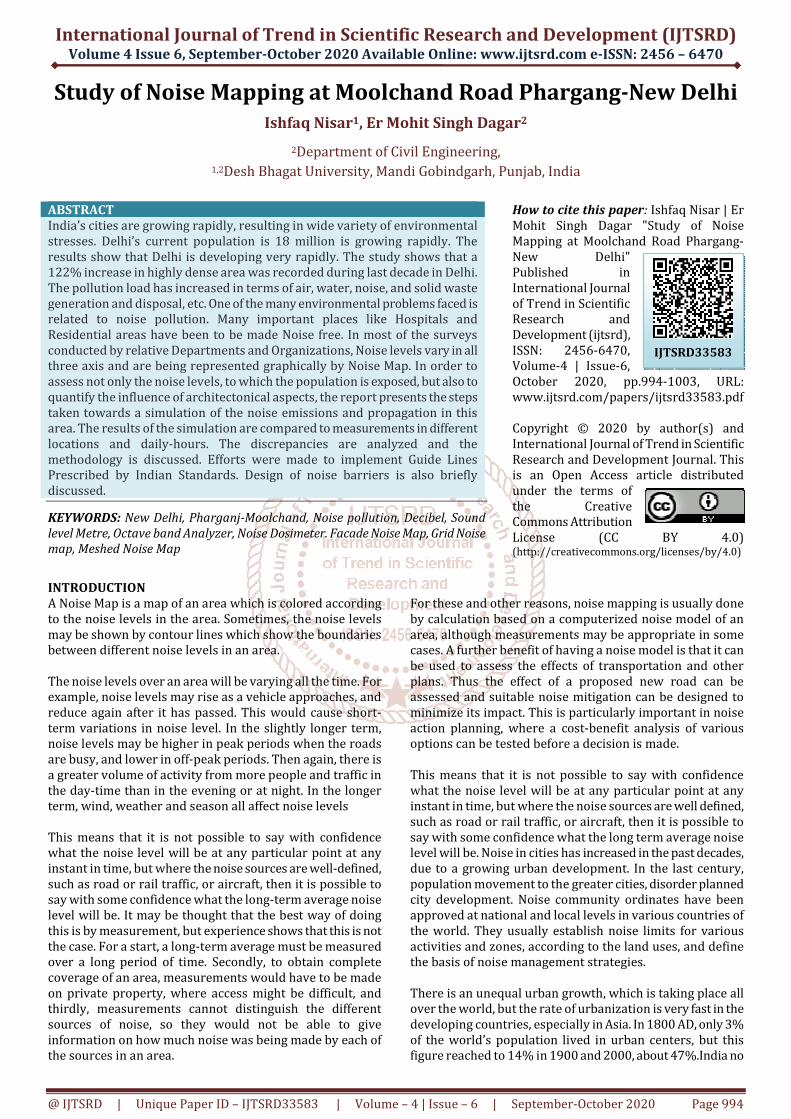
Sound Level Meters

Figure Showing Sound Level Meter

A sound level meter or sound meter is an instrument that

measures sound pressure level, commonly used in noise

pollution studies for the quantification of different kinds of

noise, especially for industrial, environmental and aircraft

noise. However, the reading from a sound level meter does

not correlate well to human-perceived loudness, which is

better measured by a loudness meter. Sound level meters

provide instantaneous noise measurements for screening

purposes. During an initial walk around, a sound level meter

helps identify areas with elevated noise levels where full

shift noise dosimetry should be performed. Sound level

meters are useful for:

� Spot checking noise dosimeter performance .

� Determining workers noise dose when the dosimeter is

unavailable or inappropriate.

� Identifying and evaluating individual noise sources for

abatement purposes.

� Aiding in engineering control feasibility analysis for

individual noise sources being considered for

abatement.

Sound Level Meter was used in this study for checking noise

levels and finding different parameters relating noise.

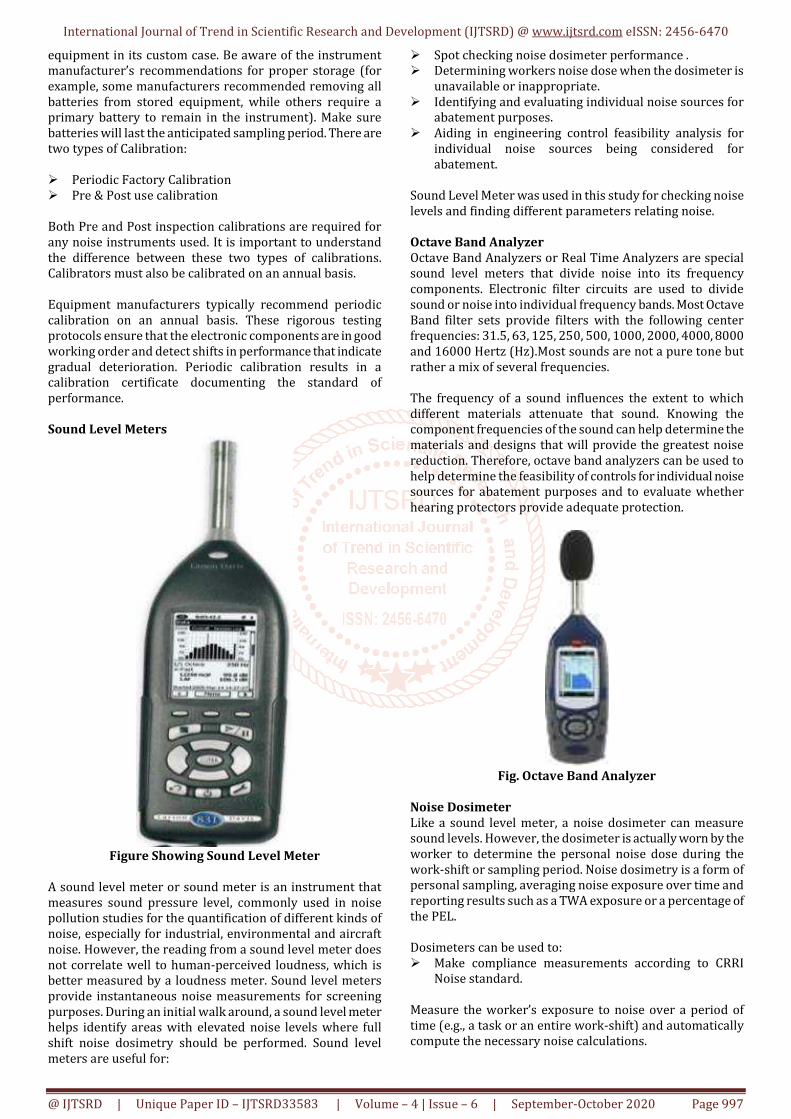
Octave Band Analyzer

Octave Band Analyzers or Real Time Analyzers are special

sound level meters that divide noise into its frequency

components. Electronic filter circuits are used to divide

sound or noise into individual frequency bands. Most Octave

Band filter sets provide filters with the following center

frequencies: 31.5, 63, 125, 250, 500, 1000, 2000, 4000, 8000

and 16000 Hertz (Hz).Most sounds are not a pure tone but

rather a mix of several frequencies.

The frequency of a sound influences the extent to which

different materials attenuate that sound. Knowing the

component frequencies of the sound can help determine the

materials and designs that will provide the greatest noise

reduction. Therefore, octave band analyzers can be used to

help determine the feasibility of controls for individual noise

sources for abatement purposes and to evaluate whether

hearing protectors provide adequate protection.

Fig. Octave Band Analyzer

Noise Dosimeter

Like a sound level meter, a noise dosimeter can measure

sound levels. However, the dosimeter is actually worn by the

worker to determine the personal noise dose during the

work-shift or sampling period. Noise dosimetry is a form of

personal sampling, averaging noise exposure over time and

reporting results such as a TWA exposure or a percentage of

the PEL.

Dosimeters can be used to:

� Make compliance measurements according to CRRI

Noise standard.

Measure the worker’s exposure to noise over a period of

time (e.g., a task or an entire work-shift) and automatically

compute the necessary noise calculations.



Figure Noise dosimeter

Types of Noise Maps

This section offers a glimpse of the noise maps. There are

three types of noise maps

1. The Facade Noise Map

2. The Grid Noise Map and

3. The Meshed Noise Map

The Facade Noise Map:

The Facade Noise Map places and calculates receivers along

the façades of buildings. Receivers can be placed every floor

with either a fixed number of receivers per facade or a set

spacing between them. The results are used for two main

purposes; to show noise levels at buildings and to generate

the data for the end noise statistics where the exposed

people are tailed. From the building the receivers are

attached to the receivers “know” the type of building, the

status of the noise control and the number of inhabitants per

building / floor. This Facade Noise Map is a great tool for

noise planning as it directly allows statistics and graphics to

be generated from a single calculation. The entire building

can be painted in the maximum noise level found anywhere

on the outside, facades can be marked if they exceed the

allowable noise limit, individual receivers can indicate an

infringement of the limits by using different symbols below /

above the limit. The Façade Noise Map like any other noise

map in Sound PLAN allows to be displayed as a regular map

projected on the floor plan or as a rendered 3D model.

The Grid Noise Map:

The Grid Noise Map comes in two variants, as a horizontal

map (Grid Noise Maps) where the receivers follow the

terrain or in the vertical format as Cross-sectional Noise

Map. Spacing of receivers and height above the ground are

user selectable. There is no size limit for Grid Noise Maps,

however as Sound PLAN can load an unlimited number of

Grid Noise Maps into each sheet, it is probably wise to

partition the Grid Noise maps for very big areas. Grid Noise

Maps have a whole gambit of output options to generate

contour lines and smooth them or to leave the grid in place

and show the values or have the grid painted in a fluid scale.

Cross-sectional Noise Maps are noise maps that start at the

terrain and reach to a user selected height, again the receiver

spacing us user defined. This mapping option is very user

friendly allowing the calculation to be interrupted and

resume later on or to calculate a new grid or to re-calculate

only part of the grid. If the single PC with multi-threaded

calculation proves to take too long for the job, with

Distributed Computing (DC description is under Tools) the

application is scalable to the need of the user.

The Meshed Map:

The Meshed Map is similar to the Grid Noise Map as it is a

mapping option to follow the terrain horizontally but instead

of having a fixed grid of receivers, the receivers are located

on the nodes of a mesh. The Meshed Map has two prime

applications. The first is to calculate the noise in cities with

very narrow streets. In order to obtain sensible contour

lines, the grid spacing needs to be narrow thus creating a

huge file and causing long calculation times. The Meshed

Map helps by generating more receivers where it is needed

(around sources and obstacles) and having a thinner base

mesh. This way the density of calculated receivers is higher

where the noise levels are changing rapidly and less

receivers for the rest. The Meshed Map has proved itself

invaluable in the noise mapping cities with small streets. The

second strong point of the Meshed Map is its capability to

store more information than just the noise levels for day,

evening and night. Calculate a Meshed Map once and display

multiple maps depicting singular frequencies or frequency

bands. This particular feature is especially helpful for

industrial noise control where it is often necessary to

document a noise map frequency by frequency.

Results

1. KAILASH COLONY:

Day:

Time L10 L50 L90 SEL LEQ MaxL

6-7 72.9 68.6 63.4 107.8 70.4 93.4

7-8 80 72.4 65.4 109.5 76.2 94.2

8-9 81.4 74.3 67.8 110.2 78.1 95.7

9-10 82.7 75.7 68.7 110.8 79.6 96.3

10-11 82.2 75.7 68.7 112.8 78.9 100.2

11-12 81.2 75.2 69.2 113.7 78.3 107.9

12-13 81.2 75.2 68.7 113.6 78.2 99.4

13-14 81.2 74.7 68.2 113.3 77.9 97.4

14-15 80.7 74.7 68.7 111.6 77.2 92.6

15-16 80.7 75.2 69.2 113.4 77.6 97.9

16-17 81.2 75.7 69.7 108.2 78.1 99.3

17-18 81.2 75.2 70.2 107.6 78.5 96

18-19 81.9 76.1 73.5 107.2 77.8 107.2



19-20 79.9 75.3 69.4 95.5 78.1 89.4

20-21 80.2 73.7 68.2 112.7 77.2 98.6

212-2 79.7 73.7 67.7 112.5 76.7 101.9

80.51875 68.54375 77.425 97.9625

Night:


22-23 78.7 72.7 68.2 107.5 70.3 93.1

23-24 77.4 72.6 63.2 95.2 74.5 86.6

0-1 73.7 67.9 60 106 70.5 90.2

1-2 74 68.2 61.7 106.5 71.5 88

2-3 74.7 66.7 58.6 106.5 71 88.3

3-4 65.1 62.8 58 101.4 63.2 82.1

4-5 63.8 58.9 54.4 95.2 60.6 76.9

5-6 68.2 63.1 59.2 112 65.2 92.4

71.95 60.4125 68.35 87.2

2. NEHRU VIHAR:


0-1 75.7 72.7 64.2 112.7 72.5 100.5

1-2 70.2 65.8 61 102.2 67.9 92.1

2-3 69.2 63.9 59 110.7 64.8 98.9

3-4 67.3 62.2 58.2 99 64.2 91.7

4-5 64.3 61.9 53.4 97.2 62.2 77.9

5-6 68.9 63.1 59.1 101.4 63.8 96

6-7 68.4 65.2 60.1 101.8 66.5 101.5

7-8 79.2 76.2 67.8 110 77.2 89.9

8-9 80.9 75.5 66.8 111.2 78.6 100.2

9-10 83.1 77.9 71.4 95.5 80.5 89

10-11 80.7 76.1 68.4 111.4 78.5 111.7

11-12 78.2 76.4 65.8 101.8 77.4 101.6

12-13 79.4 76.5 64.9 100.8 77.3 100.5

13-14 76.6 73.1 67.2 111.5 74.4 92.5

14-15 77.9 74.5 66.6 111.1 76.4 98.1

15-16 75.5 73.1 65.3 89.5 75.5 74.6

16-17 78.7 72.2 65.7 113.4 77.9 101.3

17-18 78 72.9 67.5 111.1 76.7 101.7

18-19 78.9 75.8 64.8 100.5 77.6 94.5

19-20 77.7 73.4 66.6 111.2 75.5 95.5

20-21 78.9 75.2 67.1 110.2 77.9 100.2

21-22 76.9 74.1 65.9 110.5 75.6 98.7

22-23 77.8 72.3 67.3 110.1 74.7 94

23-24 76.5 72.1 67.1 110.2 73.6 97.4

73.633333 95.83333

Day:


6-7 68.4 65.2 60.1 101.8 66.5 101.5

7-8 79.2 76.2 67.8 110 77.2 89.9

8-9 80.9 75.5 66.8 111.2 78.6 100.2

9-10 83.1 77.9 71.4 95.5 80.5 89

10-11 80.7 76.1 68.4 111.4 78.5 111.7

11-12 78.2 76.4 65.8 101.8 77.4 101.6

12-13 79.4 76.5 64.9 100.8 77.3 100.5

13-14 76.6 73.1 67.2 111.5 74.4 92.5

14-15 77.9 74.5 66.6 111.1 76.4 98.1

15-16 75.5 73.1 65.3 89.5 75.5 74.6

16-17 78.7 72.2 65.7 113.4 77.9 101.3

17-18 78 72.9 67.5 111.1 76.7 101.7

18-19 78.9 75.8 64.8 100.5 77.6 94.5

19-20 77.7 73.4 66.6 111.2 75.5 95.5

20-21 78.9 75.2 67.1 110.2 77.9 100.2

21-22 76.9 74.1 65.9 110.5 75.6 98.7

78.0625 66.36875 76.46875 96.96875



Night:


22-23 77.8 72.3 67.3 110.1 74.7 94

23-24 76.5 72.1 67.1 110.2 73.6 97.4

0-1 75.7 72.7 64.2 112.7 72.5 100.5

1-2 70.2 65.8 61 102.2 67.9 92.1

2-3 69.2 63.9 59 110.7 64.8 98.9

3-4 67.3 62.2 58.2 99 64.2 91.7

4-5 64.3 61.9 53.4 97.2 62.2 77.9

5-6 68.9 63.1 59.1 101.4 63.8 96

71.2375 61.1625 67.9625 93.5625

3. ASHRAM FLYOVER:


0-1 77.8 71.8 66.3 110 73.5 91.7

1-2 76.3 71.8 65.8 110.2 73.8 90.7

2-3 69.1 64.2 59.4 101.3 66.1 97.8

3-4 67.6 61.9 56.7 102.8 64.3 96.2

4-5 64.3 61.9 53.4 97.2 62.2 77.9

5-6 68.9 63.1 59.1 101.4 63.8 96

6-7 68.4 65.2 60.1 101.8 66.5 101.5

7-8 79.2 76.2 67.8 110 77.2 89.9

8-9 80.4 76.1 68.6 101.1 78.4 101.6

9-10 82.9 78.3 71.4 95.5 80.1 89

10-11 82.7 77.2 73.2 115.5 80.3 103.3

11-12 78.2 76.4 65.8 101.8 77.4 101.6

12-13 79.4 76.5 64.9 100.8 77.3 100.5

13-14 76.6 73.1 67.2 111.5 74.4 92.5

14-15 77.9 74.5 66.6 111.1 76.4 98.1

15-16 76.5 72.4 64 110.2 74.7 92.6

16-17 75.5 71.8 66.2 100.1 73.7 97.6

17-18 80.2 76.6 67.2 109.1 78.1 105.2

18-19 80.3 75.8 68.5 111.5 77.1 100.6

19-20 77.7 73.4 66.6 111.2 75.5 95.5

20-21 77.4 73.6 67.7 75.2 75.2 75.7

21-22 76.9 74.1 65.9 110.5 75.6 98.7

22-23 69.2 66.1 59.9 111.1 67.6 100.1

23-24 67.8 64.4 58.8 100.2 65.3 99.9

73.104167 95.591667

Day:


6-7 68.4 65.2 60.1 101.8 66.5 101.5

7-8 79.2 76.2 67.8 110 77.2 89.9

8-9 80.4 76.1 68.6 101.1 78.4 101.6

9-10 82.9 78.3 71.4 95.5 80.1 89

10-11 82.7 77.2 73.2 115.5 80.3 103.3

11-12 78.2 76.4 65.8 101.8 77.4 101.6

12-13 79.4 76.5 64.9 100.8 77.3 100.5

13-14 76.6 73.1 67.2 111.5 74.4 92.5

14-15 77.9 74.5 66.6 111.1 76.4 98.1

15-16 76.5 72.4 64 110.2 74.7 92.6

16-17 75.5 71.8 66.2 100.1 73.7 97.6

17-18 80.2 76.6 67.2 109.1 78.1 105.2

18-19 80.3 75.8 68.5 111.5 77.1 100.6

19-20 77.7 73.4 66.6 111.2 75.5 95.5

20-21 77.4 73.6 67.7 75.2 75.2 75.7

21-22 76.9 74.1 65.9 110.5 75.6 98.7

78.1375 66.98125 76.11875 96.49375



Night:


22-23 69.2 66.1 59.9 111.1 67.6 100.1

23-24 67.8 64.4 58.8 100.2 65.3 99.9

0-1 77.8 71.8 66.3 110 73.5 91.7

1-2 76.3 71.8 65.8 110.2 73.8 90.7

2-3 69.1 64.2 59.4 101.3 66.1 97.8

3-4 67.6 61.9 56.7 102.8 64.3 96.2

4-5 64.3 61.9 53.4 97.2 62.2 77.9

5-6 68.9 63.1 59.1 101.4 63.8 96

70.125 59.925 67.075 93.7875

Noise Mapping (Horizontal / Vertical Linear Mapping) at Ashram Chocwk

Average density of people living in 100sr yard in Delhi = 4.7

No. of dwelling unit affected in CSIR apartment, Ashram = 72

Hence, No. of people affected from >70 dB(A) noise = 72* 4.7 = 339 people



Figure: Noise Mapping at Intersection at various hours of Day


@ IJTSRD | Unique Paper ID – IJTSRD33583 | Volume – 4 | Issue – 6 | September-October 2020 03

CONCLUSION

The critical issues and challenges of development and

management for growing urban centres like Delhi, Mumbai,

and Kolkata have been the subject of extensive discussions

and debates in recent years. The major problems associated

with urban centres in India is that of unplanned expansion,

changing land use/land cover, loss of productive agricultural

land, increasing rainfall runoff, and depletion of the water

table. It is evident from the foregoing study that major urban

environmental problems occur due to high population

growth (the 46.31% increase during 1991-2001) and the

uncontrolled and mismanaged urban expansion which has

led to the doubling of the densely built-up area during last

decade in Delhi. There is a reduction (16.8%) in agricultural

land because of urban expansion in the fringe areas.

Pollution loads affecting the air, water and land in Delhi have

also increased considerably, and average night-time

temperatures (so-called “heat pollution”) have increased

significantly. The results in this work demonstrate that the

environmental noise is an important issue in New Delhi. The

studied sector, which is characterized by a high population

density and heavy traffic of vehicles from different kinds,

present background levels higher than the recommended by

the regulations applicable. The analysis of the results shows

that the noise levels in all the measured points in New Delhi,

and as can be seen from the noise map, in a large area of the

neighborhood are over the allowed values. The main cause

being the traffic noise. The technology of noise mapping

demonstrates to be an excellent means to deal with the

problem of noises pollution. The simulations are powerful

tools to be used in the urban planning. Many parameters

must be known previously or be identified to serve as base

for the correct representation of the physical effect.

Nevertheless the most laborious, like topography and

buildings, can be input to the program almost automatically

from CAD and other related softwares. The correct modeling

of the sound sources plays the most important role in the

results. The noise maps in small scale, as in the case of New

Delhi, constitutes a real important first step for a future work

in the whole city. Another important thing to be considered

in future works, is the study of the number of inhabitants

who are affected by the noise levels.

REFERENCES:

[1] Internet.

[2] Census of India (1991, 2001 and 2011) Provisional

Population Totals, Office of Registrar General of India,

Government of India, New Delhi.

[3] Passchier-Vermeer W, Passchier WF (2000) Noise

exposure and public health.

[4] Environ Health Perspect 108(6):123–131.

[5] Dr Naseem Akhtar(Senior scientist CSIR- CRRI)-

project report on noise mapping of Delhi, (2010)

[6] Niessen ME (2010) Context-based sound event

recognition. PhD Thesis, Rijksuniversiteit Groningen

[7] Ouis D (2001) Annoyance from road traffic noise: a

review. J Environ Psychol21 (1):101–120.

[8] Pe Oguntunde (2019) A study of noise pollution

measurements and possible effects on public health

[9] S Ismail (2018) Noise pollution and its sources and

effects.

[10] S Srivastava (2012) Effects of noise pollution and its

solution through eco friendly control devices.

study of noise mapping at moolchand road phargang new delhi

Education

civil engineering

new delhi

pharganj moolchand