study of gravity - intalek · hi jill - your reference boe021510-074 "study of gravity...
TRANSCRIPT

EOT_RT_template.ppt | 1/6/2009 | 1
BOEING is a trademark of Boeing Management Company.
Copyright © 2009 Boeing. All rights reserved.
(BOE021510-074)
MIKE GAMBLE2/24/10
STUDY OF GRAVITY
(CONTINUED part 2)
(SPESIF) Space Propulsion and
Energy Science International Forum
Mg10
Page 1

EOT_RT_template.ppt | 2
Engineering, Operations & Technology | Boeing Research & Technology
Copyright © 2009 Boeing. All rights reserved.
BOEING Release Memo
Sent: Tue 2/23/2010 12:13 PM
From: EXT-Pinkston, Patricia
To: Gamble, Michael A
Subject: Approved for Release: BOE021510-074
Hi Jill - Your reference BOE021510-074 "Study of Gravity part2" has been approved for Public Release.
Attached is a copy of your Approved "signed" ROI form.
<< File: GravityPrst2.ppt >>
IMPORTANT: Please keep all copies of the signed release documents (as these will be necessary if you submit another paper of a related topic).
Thank you and congratulations,
Patricia Pinkston staff analyst
BR&T Public Release requests processed (10am-12pm & 2-4pm)
Administrative Assistant to Robert Graham (Director) ECAST
ECAST, Electromagnetic Effects Technology M/C 42-22
Desk: (206) 544-7524 | Fax: (206) 544-4753
Mg10
Page 1A
EOT_RT_template.ppt | 3
Engineering, Operations & Technology | Boeing Research & Technology
Copyright © 2009 Boeing. All rights reserved.
SPESIF PITCH NOTES 2/24/10
Figure 1A) This is the Boeing memo allowing the “Public Domain” release of this “Study of Gravity” (part 2). All Boeing documents have to be reviewed and approved
before they can be presented or published.
EOT_RT_template.ppt | 4
Engineering, Operations & Technology | Boeing Research & Technology
Copyright © 2009 Boeing. All rights reserved.
STUDY OF GRAVITY (cont)
INTRODUCTION Hello, my name is Mike Gamble, I am an electronics engineer for The Boeing
Co. (Seattle). Would like to thank the chair person for having me back to
present (part2) as the (part1) presentation of gravity was from a very different perspective, more of a macroscopic overview.
HISTORYAt last year’s SPESIF conference I presented the “Study of Gravity” (part1).
Starting with documentation of existing relevant data about gravity. Then
proceeded with the mathematical analysis concluding with a four wave harmonic
dipole accelerating field model. This presentation the “Study of Gravity” (part2)
continues the mathematical analysis of gravity concluding with electromagnetic
field equations of that same model. As some may not have seen last year’s presentation I have included a few charts from (part1) for review.
Mike Gamble ([email protected])
Mg10
Page 2

EOT_RT_template.ppt | 5
Engineering, Operations & Technology | Boeing Research & Technology
Copyright © 2009 Boeing. All rights reserved.
Tutorials• Schumann Resonance• DC/AC Dipoles • Traveling /Standing Waves
• Acceleration data plot conversions:• X(equator) and Y(polar) to cylindrical coordinates• English to metric units• Most (EM) electromagnetic equations are in metric
units and spherical coordinates
• E-field, B-field and F-field wave generation• Gravity conclusions• Proposed space drives
Steps in Understanding Gravity
Mg10
Page 3

EOT_RT_template.ppt | 6
Engineering, Operations & Technology | Boeing Research & Technology
Copyright © 2009 Boeing. All rights reserved.
Figure 3) “Steps in Understanding Gravity” is an outline of the tasks preformed in
part 2. It contains three tutorials and the main section on (EM) ElectroMagnetic field generation followed by a couple of proposed space drives. The first tutorial is a more in depth study of Schumann resonance as part 1 only mentioned it in passing.
The second tutorial is on basic DC and AC dipoles including their detailed EM equations. The third tutorial is a detailed study of EM traveling and standing waves
as they apply to this study. The main section on EM field generation takes the
acceleration equations created in part 1 and converts them to cylindrical coordinates
and metric units. This change makes the mathematics somewhat easier to work with as standard EM field equations are metric but in spherical coordinates. Part 2
concludes with a working EM accelerating force (gravity) equation which has very
good correlation to the original proposed data from part 1. The presentation concludes with a couple of proposed space drives based on this information.

EOT_RT_template.ppt | 7Copyright © 2009 Boeing. All rights reserved.
SCHUMANN RESONANCE
Mg10
Page 4
EOT_RT_template.ppt | 8
Engineering, Operations & Technology | Boeing Research & Technology
Copyright © 2009 Boeing. All rights reserved.
Figure 4) “Schumann Resonance” is a short tutorial on the subject of resonate
waves and how they apply to this “Study of Gravity”. It takes a more detailed look at what these waves contribute to the earth’s operating system.

EOT_RT_template.ppt | 9
Engineering, Operations & Technology | Boeing Research & Technology
Copyright © 2009 Boeing. All rights reserved.
Spherical EM Resonate Cavity
Conductive Surfaces (Rin, Rout)
Radius (mean)
Fn = c [n(n+1)]^0.5 [µµµµr / εεεεr]^0.5
2ππππRm
Equation Terms
Fn = Freq of osc
c = Speed of light
Rm = Radius (mean)
n = Harmonic number
µµµµr = Magnetic permeability
εεεεr = Electric permittivity
εr µr
Cavity Dielectric and permeability
Rout
Rin
Rm
Open Ended Cavity Supports All Harmonics
Mg10
Page 5

EOT_RT_template.ppt | 10
Engineering, Operations & Technology | Boeing Research & Technology
Copyright © 2009 Boeing. All rights reserved.
Figure 5) “Spherical EM Resonate Cavity” is the standard textbook definition of a 3D
circular (spherical) EM cavity oscillator. It will support all harmonic frequencies (fundamental, second, third, fourth, etc) as it is an open ended tuned structure.
The cavity is composed of a dielectric media located between two electrically conductive surfaces. As it is circular in shape the transfer function uses the
average radius (Rm) of the two surface radiuses (Rin, Rout). From the equation it
can be seen that the frequency is determined by three variables: the mean radius
(Rm), the electric permittivity (εεεεr) and the magnetic permeability (µµµµr).
Main points:
1) Open ended 3D tuned structure
2) Composed of a dielectric media between two conductors
3) Frequency is controlled by three variables: Rm, εεεεr and µµµµr

EOT_RT_template.ppt | 11
Engineering, Operations & Technology | Boeing Research & Technology
Copyright © 2009 Boeing. All rights reserved.
EARTH’S RESONATE CAVITY
733Miles
733 Miles
2160 Miles
OUTERCORE
MANTLEATMOSPHERE
SURFACE (Re)
CRUST
INNER CORE
IONOSPHERE
CRUST
0
air
3943 Miles
3963 Miles
4013 Miles
4194 Miles
Rout = 4063Miles (outer)
Rm = 4013Miles (mean)(Re) Rin = 3963Miles (inner)
Rout
Rm
Rin
4063 Miles
Mg10
Page 6
EOT_RT_template.ppt | 12
Engineering, Operations & Technology | Boeing Research & Technology
Copyright © 2009 Boeing. All rights reserved.
Figure 6) “Earth’s Resonate Cavity” shows the location of this cavity as it applies to
the earth’s system. The inner radius (Rin) is the earths surface (Re) as the crust
is conductive. And the outer radius (Rout) is about the middle of the ionosphere where it is conductive around a 100miles out. That places the mean radius (Rm)
around 50 miles or about the outer edge of the atmosphere. The magnetic
permeability for most nonferrous materials like air is about (µµµµr = 1) and the
dielectric electric constant of air is (εεεεr = 1).
Main points:
1) Structure of earths cavity
2) Conductive surfaces are the crust and the ionosphere3) Cavity mean radius is the edge of the atmosphere
4) Dielectric media constants: εεεεr= 1 and µµµµr= 1

EOT_RT_template.ppt | 13
Engineering, Operations & Technology | Boeing Research & Technology
Copyright © 2009 Boeing. All rights reserved.
Earth’s Resonate CavityCalculations
Plugging the numbers into the textbook equation
F1 = 186,284(miles/sec) * [1([1]+1)]^.5 * [1/1]^.5 / 2ππππ4013(miles) Hz= 10.45Hz (perfect resonator)
Higher then Schumann Resonance of 7.83Hz
For a leaky (less then perfect) resonate cavity: gain/offset terms must be empirically
adjusted [n(1*n+1) to n(.689n+.433)]. Outer conductor (ionosphere) has day/night variations, Dielectric (not homogeneous) arcs/sparks (lightning), Inner conductor
(planet surface) composed of different materials soil and water. Soil not smooth
contains mountains and valleys.
Fn = 186,284(miles/sec)[n(.689n+.433)]^.5 / 2ππππ4013(miles) Hz
Schumann frequency numbers with the modified equation:F1 = 7.83Hz (fundamental)
F2 = 14.07Hz (second)
F3 = 20.25Hz (third)
F4 = 26.41Hz (fourth)
Mg10
Page 7
EOT_RT_template.ppt | 14
Engineering, Operations & Technology | Boeing Research & Technology
Copyright © 2009 Boeing. All rights reserved.
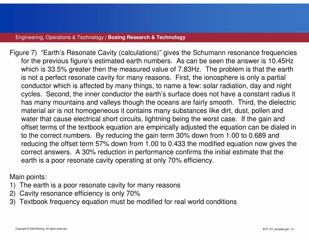
Figure 7) “Earth’s Resonate Cavity (calculations)” gives the Schumann resonance frequencies for the previous figure’s estimated earth numbers. As can be seen the answer is 10.45Hz
which is 33.5% greater then the measured value of 7.83Hz. The problem is that the earth is not a perfect resonate cavity for many reasons. First, the ionosphere is only a partial conductor which is affected by many things, to name a few: solar radiation, day and night
cycles. Second, the inner conductor the earth’s surface does not have a constant radius it has many mountains and valleys though the oceans are fairly smooth. Third, the dielectric
material air is not homogeneous it contains many substances like dirt, dust, pollen and water that cause electrical short circuits, lightning being the worst case. If the gain and
offset terms of the textbook equation are empirically adjusted the equation can be dialed in to the correct numbers. By reducing the gain term 30% down from 1.00 to 0.689 and
reducing the offset term 57% down from 1.00 to 0.433 the modified equation now gives the correct answers. A 30% reduction in performance confirms the initial estimate that the
earth is a poor resonate cavity operating at only 70% efficiency.
Main points:1) The earth is a poor resonate cavity for many reasons2) Cavity resonance efficiency is only 70%
3) Textbook frequency equation must be modified for real world conditions

EOT_RT_template.ppt | 15
Engineering, Operations & Technology | Boeing Research & Technology
Copyright © 2009 Boeing. All rights reserved.
Earth’s Resonate CavityCalculations (cont)
If the driving freq (Fdr) is in the half power band (3db – “Q”point) of a resonant cavity [freq (Fosc)] there is full energy transfer (gain = 100%). The further Fdr is from the “Q”point the less energy transferred.
Fosc “Q”band Fdr Delta Gain(fundamental) 7.83Hz +/- .5Hz 7.07Hz .76Hz 90%
(second) 14.07Hz +/- .5Hz 14.14Hz .07Hz 100%
(third) 20.25Hz +/- .5Hz 21.21Hz .96Hz 60%
(fourth) 26.41Hz +/- .5Hz 28.28Hz 1.87Hz 30%
Mg10
Page 8
EOT_RT_template.ppt | 16
Engineering, Operations & Technology | Boeing Research & Technology
Copyright © 2009 Boeing. All rights reserved.
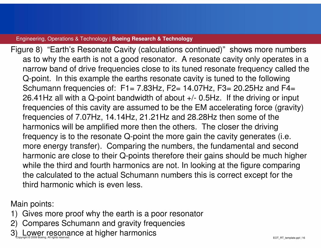
Figure 8) “Earth’s Resonate Cavity (calculations continued)” shows more numbers as to why the earth is not a good resonator. A resonate cavity only operates in a narrow band of drive frequencies close to its tuned resonate frequency called the
Q-point. In this example the earths resonate cavity is tuned to the following
Schumann frequencies of: F1= 7.83Hz, F2= 14.07Hz, F3= 20.25Hz and F4= 26.41Hz all with a Q-point bandwidth of about +/- 0.5Hz. If the driving or input frequencies of this cavity are assumed to be the EM accelerating force (gravity)
frequencies of 7.07Hz, 14.14Hz, 21.21Hz and 28.28Hz then some of the
harmonics will be amplified more then the others. The closer the driving frequency is to the resonate Q-point the more gain the cavity generates (i.e.
more energy transfer). Comparing the numbers, the fundamental and second
harmonic are close to their Q-points therefore their gains should be much higher while the third and fourth harmonics are not. In looking at the figure comparing
the calculated to the actual Schumann numbers this is correct except for the
third harmonic which is even less.
Main points:
1) Gives more proof why the earth is a poor resonator
2) Compares Schumann and gravity frequencies
3) Lower resonance at higher harmonics
EOT_RT_template.ppt | 17
Engineering, Operations & Technology | Boeing Research & Technology
Copyright © 2009 Boeing. All rights reserved.
SCHUMANN HARMONICSPlanet Structure
733Miles
733 Miles2160 Miles
OUTERCORE
MANTLEATMOSPHERE
SURFACE (Re)
CRUST
INNER CORE
IONOSPHERE
CRUST
0
air
3943 Miles
3963 Miles
4013 Miles
4194 Miles
Radius(R) = 4194Miles (7.07Hz)
Rair = 4013Miles (7.39Hz)Re = 3963Miles (7.48Hz)
R
Rair
Re
Mg10
Page 9
Third Harmonic(20.25Hz)
Fourth Harmonic(26.41Hz)
Fifth Harmonic(32.45Hz)
1123Miles1464Miles
2107Miles
3786Miles
915Miles
Second Harmonic(14.07 Hz)
First Harmonic(7.83Hz)
EOT_RT_template.ppt | 18
Engineering, Operations & Technology | Boeing Research & Technology
Copyright © 2009 Boeing. All rights reserved.
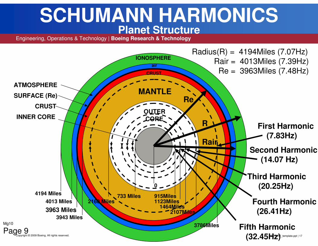
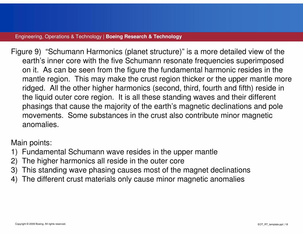
Figure 9) “Schumann Harmonics (planet structure)” is a more detailed view of the
earth’s inner core with the five Schumann resonate frequencies superimposed
on it. As can be seen from the figure the fundamental harmonic resides in the mantle region. This may make the crust region thicker or the upper mantle more
ridged. All the other higher harmonics (second, third, fourth and fifth) reside in the liquid outer core region. It is all these standing waves and their different
phasings that cause the majority of the earth’s magnetic declinations and pole
movements. Some substances in the crust also contribute minor magnetic anomalies.
Main points:1) Fundamental Schumann wave resides in the upper mantle
2) The higher harmonics all reside in the outer core
3) This standing wave phasing causes most of the magnet declinations
4) The different crust materials only cause minor magnetic anomalies

EOT_RT_template.ppt | 19Copyright © 2009 Boeing. All rights reserved.
DC and AC EM Dipoles
Mg10
Page 10
EOT_RT_template.ppt | 20
Engineering, Operations & Technology | Boeing Research & Technology
Copyright © 2009 Boeing. All rights reserved.
Figure 10) “DC and AC (EM) ElectroMagnetic Dipoles” is a short tutorial on different types of dipoles. Starting with a description of a simple DC electric dipole
and its equations then proceeding to a more complex AC magnetic dipole and its equations. This is background material for understanding the interactions between
an accelerating force field and the electric and magnetic fields.

EOT_RT_template.ppt | 21
Engineering, Operations & Technology | Boeing Research & Technology
Copyright © 2009 Boeing. All rights reserved.
ELECTRIC DIPOLE (DC)
The V electric potential fields radiate
outward (radial) from each pole decreasing
with distance (radius). Polarity of +V field
being the equal and opposite of –V field.
The difference (gradient) field between the
two pole potentials is the E electric field which
has components Er in the radial direction and
Ez in the axial direction.
The curl of the E electric field is the Bθθθθ
magnetic field which would be in the circular
(theta) direction except its zero. As the E field
is constant (DC).
D
+V
-V
EE
Mg10
Page 11
EOT_RT_template.ppt | 22
Engineering, Operations & Technology | Boeing Research & Technology
Copyright © 2009 Boeing. All rights reserved.
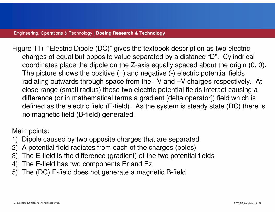
Figure 11) “Electric Dipole (DC)” gives the textbook description as two electric
charges of equal but opposite value separated by a distance “D”. Cylindrical
coordinates place the dipole on the Z-axis equally spaced about the origin (0, 0). The picture shows the positive (+) and negative (-) electric potential fields radiating outwards through space from the +V and –V charges respectively. At
close range (small radius) these two electric potential fields interact causing a
difference (or in mathematical terms a gradient [delta operator]) field which is
defined as the electric field (E-field). As the system is steady state (DC) there is no magnetic field (B-field) generated.
Main points:1) Dipole caused by two opposite charges that are separated
2) A potential field radiates from each of the charges (poles)
3) The E-field is the difference (gradient) of the two potential fields
4) The E-field has two components Er and Ez
5) The (DC) E-field does not generate a magnetic B-field
EOT_RT_template.ppt | 23
Engineering, Operations & Technology | Boeing Research & Technology
Copyright © 2009 Boeing. All rights reserved.
ELECTRIC DIPOLE (DC)[equations]
V = Electric Potential (cyl)
V = K [1 / (r^2+ (z-D/2)^2)^.5
- 1 / (r^2+(z+D/2)^2)^.5]
E = Electric Field (cyl)
E = - V Gradient of Electric Potential
Er = K [r / (r^2+ (z-D/2)^2)^1.5
- r / (r^2+(z+D/2)^2)^1.5]Ez = K [(z-D/2) / (r^2+(z-D/2)^2)^1.5
- (z+D/2) / (r^2+(z+D/2)^2)^1.5]
B = Magnetic Field (cyl)
B = -jωεµωεµωεµωεµ x E Curl of Electric FieldBθθθθ = 0
Mg10
Page 12

EOT_RT_template.ppt | 24
Engineering, Operations & Technology | Boeing Research & Technology
Copyright © 2009 Boeing. All rights reserved.
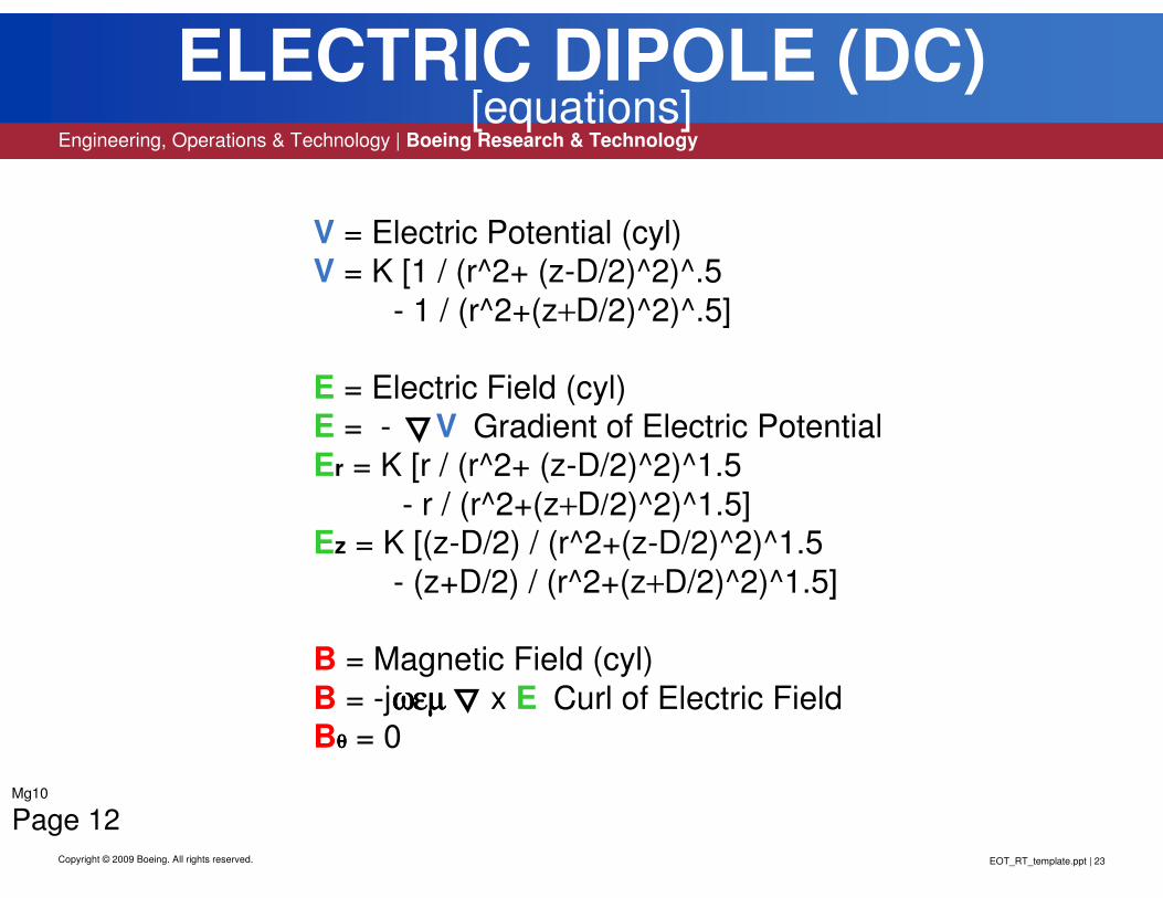
Figure 12) “Electric Dipole (DC equations)” is the full set of mathematical equations in cylindrical (cyl) coordinates that define these fields. They are composed of two
interrelated terms. First, is the electric potential (V) which is measured in “volts” and decreases in value inversely as the distance (1/R). Because a dipole has two opposite
polarities the equation also carries two terms one positive and one negative. Second, the electric field (E) is defined as the negative gradient [delta (or difference) operator] of the
electric potential (V). It is measured in “volts/meter” and decreases in value inversely as the square of the distance (1/R^2). The gradient operation produces two terms (Er) in the R-axis and (Ez) in the Z-axis. Both of these equations also carry the two dipole polarity
terms one positive and one negative. The magnetic field (B) is defined as the negative curl (delta vector cross product) of the electric field. As it is steady state or DC the
frequency term (ω= 0). Note the “gradient” and “curl” operations are standard calculus mathematical procedures.
Main points:
1) Full set of equations defining the DC electric dipole2) Each equation carries a positive and negative term
3) The E-field attenuates inversely as the square if the distance (1/R^2), units being [volts/meter]
4) The E-field has components in both the R and Z axis
5) Frequency term (ω) equals zero for DC

EOT_RT_template.ppt | 25
Engineering, Operations & Technology | Boeing Research & Technology
Copyright © 2009 Boeing. All rights reserved.
MAGNETIC DIPOLE (DC)
The Aθθθθ magnetic potential field is in the
circular (theta) direction.
The curl of the A magnetic potential is
the B magnetic field which has components
Br in the radial direction and Bz in the axial
direction.
The curl of the B magnetic field is the Eθθθθ
electric field which would be in the circular
(theta) direction except its zero. As the B field
is constant (DC).
Field spins in the circular (theta) direction.
Frequency is determined by dipole length.
λ / 2
N
S
BAB
Spin
Mg10
Page 13

EOT_RT_template.ppt | 26
Engineering, Operations & Technology | Boeing Research & Technology
Copyright © 2009 Boeing. All rights reserved.
Figure 13) “Magnetic Dipole (DC)” gives the textbook description as two magnetic
potentials of equal but opposite value separated by a distance (λ/2). Cylindrical coordinates place the dipole on the Z-axis equally spaced about the origin (0, 0).
The picture shows the positive (+) and negative (-) magnetic potential fields
radiating (spinning) outwards through space from the “N” and “S” poles respectively. At close range (small radius) these two magnetic potential fields
interact causing a difference (or in mathematical terms a gradient [delta
operator]) field which is defined as the magnetic field (B-field). As the system is
steady state (DC) there is no electric field (E-field) generated. The major
difference between the magnetic and electric DC dipoles is that the magnetic
one has a spinning field making the dipole separation distance (D) a tuned
length (λ/2).
Main points:
1) Dipole caused by two opposite poles that are separated2) A potential field radiates from each of the poles
3) The B-field is the difference (gradient) of the two potential fields
4) The B-field has two components Br and Bz
5) The (DC) B-field does not generate an electric E-field but it does spin

EOT_RT_template.ppt | 27
Engineering, Operations & Technology | Boeing Research & Technology
Copyright © 2009 Boeing. All rights reserved.
MAGNETIC DIPOLE (DC)[equations]
Aθθθθ = Magnetic Potential (cyl)
Aθθθθ = -µµµµK [(z-λλλλ/4) / (r(r^2+ (z-λλλλ/4)^2)^.5)
-(z+λλλλ/4) / (r(r^2+(z+λλλλ/4)^2)^.5)]
B = Magnetic Field (cyl)
B = x A Curl of Magnetic Potential
Br = µµµµK [r / (r^2+ (z-λλλλ/4)^2)^1.5
- r / (r^2+(z+λ/+λ/+λ/+λ/4)^2)^1.5]
Bz = µµµµK [(z-λλλλ/4) / (r^2+ (z-λλλλ/4)^2)^1.5
- (z+λλλλ/4) / (r^2+(z+λλλλ/4)^2)^1.5]
E = Electric Field (cyl)
E = (1 / jωεµωεµωεµωεµ) x B Curl of Magnetic FieldEθθθθ = 0
fθθθθ = Spin Frequency
fθθθθ = C / λ λ λ λ Hz Mg10
Page 14
EOT_RT_template.ppt | 28
Engineering, Operations & Technology | Boeing Research & Technology
Copyright © 2009 Boeing. All rights reserved.
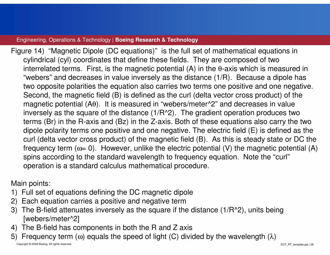
Figure 14) “Magnetic Dipole (DC equations)” is the full set of mathematical equations in
cylindrical (cyl) coordinates that define these fields. They are composed of two
interrelated terms. First, is the magnetic potential (A) in the θ-axis which is measured in “webers” and decreases in value inversely as the distance (1/R). Because a dipole has two opposite polarities the equation also carries two terms one positive and one negative.
Second, the magnetic field (B) is defined as the curl (delta vector cross product) of the
magnetic potential (Aθ). It is measured in “webers/meter^2” and decreases in value inversely as the square of the distance (1/R^2). The gradient operation produces two
terms (Br) in the R-axis and (Bz) in the Z-axis. Both of these equations also carry the two dipole polarity terms one positive and one negative. The electric field (E) is defined as the
curl (delta vector cross product) of the magnetic field (B). As this is steady state or DC the
frequency term (ω= 0). However, unlike the electric potential (V) the magnetic potential (A) spins according to the standard wavelength to frequency equation. Note the “curl”operation is a standard calculus mathematical procedure.
Main points:
1) Full set of equations defining the DC magnetic dipole2) Each equation carries a positive and negative term3) The B-field attenuates inversely as the square if the distance (1/R^2), units being
[webers/meter^2]4) The B-field has components in both the R and Z axis
5) Frequency term (ω) equals the speed of light (C) divided by the wavelength (λ)

EOT_RT_template.ppt | 29
Engineering, Operations & Technology | Boeing Research & Technology
Copyright © 2009 Boeing. All rights reserved.
DC to AC Equation Conversion
Eulers Equation converts AC (sin and cos) terms to exponentials which
are easier to work with mathematically.
exp(j[ωωωωt-2ππππr/λλλλ]) = cos(ωωωωt-2ππππr/λλλλ)+jsin(ωωωωt-2ππππr/λλλλ)
AC phaser notation uses only use the displacement term (-2ππππr/λλλλ), the
time term (ωωωωt) is dropped as the wave amplitude is assumed to oscillate.
exp(-j2ππππr/λλλλ)
Multiplying the DC field equations with the phaser adds the AC component.
The differentials now become more complicated with additional terms and
imaginary numbers.
Mg10
Page 15

EOT_RT_template.ppt | 30
Engineering, Operations & Technology | Boeing Research & Technology
Copyright © 2009 Boeing. All rights reserved.
Figure 15) “DC to AC Equation Conversion” documents the three step process that
is used to make the change to AC. First, using Euler’s formula the sine and cosine frequency terms are converted into exponential terms. In calculus
exponentials are easier to differentiate and integrate then sine and cosine terms. Second, is to reduce the equation down to AC phaser notation. EM field calculations use a simplification called AC phaser notation which uses only the
position or displacement term (-2πr/λ) of the Euler’s equation. The frequency or
time term (ωt) is dropped as an AC wave is assumed to oscillate. Third, is to multiply the DC equations by the AC phaser which completes the DC to AC conversion process. The AC equations are more difficult to differentiate as they
now have more terms to work with and also contain imaginary numbers.
Main points:
1) To convert from DC to AC is a three step process
2) Change sine/cosine terms to exponentials3) Modify exponentials to make AC phasers4) Multiply the DC equation by the phaser term
5) The AC equations are more difficult to work with

EOT_RT_template.ppt | 31
Engineering, Operations & Technology | Boeing Research & Technology
Copyright © 2009 Boeing. All rights reserved.
ELECTRIC DIPOLE (AC)
The V electric potential fields radiate
outward (radial) from each pole decreasing
with distance (radius). Polarity of +V field
being the equal and opposite of –V field.
The difference (gradient) field between the
two pole potentials is the E electric field which
has components Er in the radial direction and
Ez in the axial direction.
The curl of the E electric field is the Bθθθθ
magnetic field in the circular (theta) direction.
As the fields are AC they oscillate, the Bθθθθ
magnetic field (back and forth) in the circular
(theta) direction and the E electric field
(up and down) in the axial direction. Frequency
is determined by dipole length.
λ/2λ/2λ/2λ/2
V/-V
-V/V
EE B
Osc
Mg10
Page 16

EOT_RT_template.ppt | 32
Engineering, Operations & Technology | Boeing Research & Technology
Copyright © 2009 Boeing. All rights reserved.
Figure 16) “Electric Dipole (AC)” gives about the same textbook description as for a DC dipole that of two electric charges of equal but opposite value separated by
a distance “D” which now becomes half wavelength (λ/2). Cylindrical coordinates still places the dipole on the Z-axis equally spaced about the origin (0, 0). The picture shows the positive (+/-) and negative (-/+) electric potential fields which now oscillate radiating outwards through space from the V/-V and –
V/V charges respectively. At close range (small radius) these two electric
potential fields interact causing a difference (or in mathematical terms a gradient
[delta operator]) field which is defined as the electric field (E-field). The big difference in the AC dipole system is that it now generates an orthogonal
oscillating magnetic field (B-field) in the circular (θ) direction.
Main points:
1) Dipole caused by two opposite charges that are separated
2) The dipole separation distance is now λ/23) A potential field radiates from each of the charges4) The E-field is the difference (gradient) of the two potential fields
5) The E-field has two components Er and Ez
6) The (AC) E-field generates a magnetic B-field (Bθ) in the θ-axis

EOT_RT_template.ppt | 33
Engineering, Operations & Technology | Boeing Research & Technology
Copyright © 2009 Boeing. All rights reserved.
ELECTRIC DIPOLE (AC)
V = Electric Potential (cyl)
V = K [(1 / (r^2+(z-λλλλ/4)^2)^.5)exp(-j2ππππ(r^2+ (z-λλλλ/4)^2)^.5/λλλλ)
-(1 / (r^2+(z+λλλλ/4)^2)^.5)exp(-j2ππππ(r^2+(z+λλλλ/4)^2)^.5/λλλλ)]
E = Electric Field (cyl)
E = - A Gradient of Electric Potential
Er = K[(r /(r^2+(z-λλλλ/4)^2)^1.5+j2ππππr /(λλλλ(r^2+ (z-λλλλ/4)^2)))exp(-j2ππππ(r^2+ (z-λλλλ/4)^2)^.5/λλλλ)
-(r /(r^2+(z+λλλλ/4)^2)^1.5+j2ππππr /(λλλλ(r^2+(z+λλλλ/4)^2)))exp(-j2ππππ(r^2+(z+λλλλ/4)^2)^.5/λλλλ)]
Ez = K[((z-λλλλ/4) /(r^2+ (z-λλλλ/4)^2)^1.5+j2ππππ(z-λλλλ/4) /(λλλλ(r^2+(z-λλλλ/4)^2)))exp(-j2ππππ(r^2+ (z-λλλλ/4)^2)^.5/λλλλ)
-((z+λλλλ/4) /(r^2+(z+λλλλ/4)^2)^1.5+j2ππππ(z+λλλλ/4) /(λλλλ(r^2+(z+λλλλ/4)^2)))exp(-j2ππππ(r^2+(z+λλλλ/4)^2)^.5/λλλλ)]
B = Magnetic Field (cyl)
B = -jωεµωεµωεµωεµ x E Curl of Electric Field or E = 1 / jωεµωεµωεµωεµ x B Curl of Magnetic Field
Bθθθθ = -jωεµωεµωεµωεµK[((z-λλλλ/4) /(r(r^2+ (z-λλλλ/4)^2)^.5))exp(-2ππππ(r^2+ (z-λλλλ/4)^2)^.5/λλλλ)
-((z+λλλλ/4) /(r(r^2+(z+λλλλ/4)^2)^.5))exp(-2ππππ(r^2+(z+λλλλ/4)^2)^.5/λλλλ)]
fθθθθ = Osc Frequency
fθθθθ = C / λλλλ Hz Mg10
Page 17
EOT_RT_template.ppt | 34
Engineering, Operations & Technology | Boeing Research & Technology
Copyright © 2009 Boeing. All rights reserved.
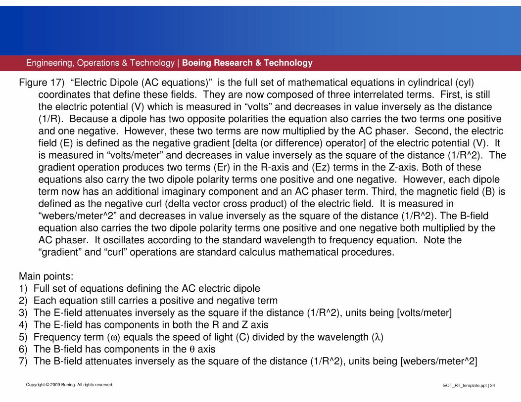
Figure 17) “Electric Dipole (AC equations)” is the full set of mathematical equations in cylindrical (cyl) coordinates that define these fields. They are now composed of three interrelated terms. First, is still
the electric potential (V) which is measured in “volts” and decreases in value inversely as the distance (1/R). Because a dipole has two opposite polarities the equation also carries the two terms one positive
and one negative. However, these two terms are now multiplied by the AC phaser. Second, the electric field (E) is defined as the negative gradient [delta (or difference) operator] of the electric potential (V). It
is measured in “volts/meter” and decreases in value inversely as the square of the distance (1/R^2). The gradient operation produces two terms (Er) in the R-axis and (Ez) terms in the Z-axis. Both of these
equations also carry the two dipole polarity terms one positive and one negative. However, each dipole term now has an additional imaginary component and an AC phaser term. Third, the magnetic field (B) is
defined as the negative curl (delta vector cross product) of the electric field. It is measured in
“webers/meter^2” and decreases in value inversely as the square of the distance (1/R^2). The B-field equation also carries the two dipole polarity terms one positive and one negative both multiplied by the
AC phaser. It oscillates according to the standard wavelength to frequency equation. Note the “gradient” and “curl” operations are standard calculus mathematical procedures.
Main points:
1) Full set of equations defining the AC electric dipole2) Each equation still carries a positive and negative term
3) The E-field attenuates inversely as the square if the distance (1/R^2), units being [volts/meter]4) The E-field has components in both the R and Z axis
5) Frequency term (ω) equals the speed of light (C) divided by the wavelength (λ)6) The B-field has components in the θ axis7) The B-field attenuates inversely as the square of the distance (1/R^2), units being [webers/meter^2]

EOT_RT_template.ppt | 35
Engineering, Operations & Technology | Boeing Research & Technology
Copyright © 2009 Boeing. All rights reserved.
MAGNETIC DIPOLE (AC)
The Aθθθθ magnetic potential field is in the
circular (theta) direction.
The curl of the A magnetic potential is
the B magnetic field which has components
Br in the radial direction and Bz in the axial
direction.
The curl of the B magnetic field is the Eθθθθ
electric field which is in the circular (theta)
direction.
As the fields are AC they oscillate, the Eθθθθ
electric field (back and forth) in a circular
(theta) direction and the B magnetic field
(up and down) in the axial direction. Frequency
is determined by dipole length.
λ / 2
N/S
S/N
BEB
Osc
Mg10
Page 18

EOT_RT_template.ppt | 36
Engineering, Operations & Technology | Boeing Research & Technology
Copyright © 2009 Boeing. All rights reserved.
Figure 18) “Magnetic Dipole (AC)” gives the same textbook description as for a DC
dipole that of two magnetic potentials of equal but opposite value separated by a
distance (λ/2). Cylindrical coordinates still places the dipole on the Z-axis equally spaced about the origin (0, 0). The picture shows the positive (+/-) and negative
(-/+) magnetic potential fields which now oscillate radiating (spinning) outwards
through space from the “N/S” and “S/N” poles respectively. At close range (small radius) these two magnetic potential fields interact causing a difference (or in
mathematical terms a gradient [delta operator]) field which is defined as the
magnetic field (B-field). The big difference in the AC system is that it now
generates an orthogonal oscillating electric field (E-field) in the circular (θ) direction.
Main points:
1) Dipole caused by two opposite poles that are separated
2) A potential field radiates from each of the poles3) The B-field is the difference (gradient) of the two potential fields4) The B-field has two components Br and Bz
5) The (AC) B-field generates an electric E-field in the θ-axis

EOT_RT_template.ppt | 37
Engineering, Operations & Technology | Boeing Research & Technology
Copyright © 2009 Boeing. All rights reserved.
MAGNETIC DIPOLE (AC)[equations]
Aθθθθ = Magnetic Potential (cyl)
Aθθθθ = -µµµµK [((z-λλλλ/4) / (r(r^2+ (z-λλλλ/4)^2)^.5))exp(-j2ππππ(r^2+ (z-λλλλ/4)^2)^.5/λλλλ)
- ((z+λλλλ/4) / (r(r^2+(z+λλλλ/4)^2)^.5))exp(-j2ππππ(r^2+(z+λλλλ/4)^2)^.5/λλλλ)] B = Magnetic Field (cyl)
B = x A Curl of Magnetic Potential
Br = µµµµK [(r / (r^2+(z-λλλλ/4)^2)^1.5
+ j2π π π π (z-λλλλ/4)^2 / (λλλλr(r^2+ (z-λλλλ/4)^2)))exp(-j2ππππ(r^2+ (z-λλλλ/4)^2)^.5/λλλλ)
- (r / (r^2+(z+λλλλ/4)^2)^1.5
+ j2ππππ(z+λλλλ/4)^2 / (λλλλr(r^2+(z+λλλλ/4)^2)))exp(-j2ππππ(r^2+(z+λλλλ/4)^2)^.5/λλλλ)]
Bz = µµµµK [(z-λλλλ/4)*(1 / (r^2+ (z-λλλλ/4)^2)^1.5
+ j2π π π π / (λλλλ(r^2+ (z-λλλλ/4)^2)))exp(-j2ππππ(r^2+ (z-λλλλ/4)^2)^.5/λλλλ)
- (z+λλλλ/4)*(1 / (r^2+(z+λλλλ/4)^2)^1.5
+ j2π π π π / (λλλλ(r^2+(z+λλλλ/4)^2)))exp(-j2ππππ(r^2+(z+λλλλ/4)^2)^.5/λλλλ)]E = Electric Field (cyl)
E = 1 / jωεµωεµωεµωεµ x B Curl of Magnetic Field
Eθθθθ = j2ππππ(µ/εµ/εµ/εµ/ε)^.5K [((z-λλλλ/4) / (λλλλr(r^2+ (z-λλλλ/4)^2)^.5))exp(-j2ππππ(r^2+ (z-λλλλ/4)^2)^.5/λλλλ)
- ((z+λλλλ/4) / (λλλλr(r^2+(z+λλλλ/4)^2)^.5))exp(-j2ππππ(r^2+(z+λλλλ/4)^2)^.5/λλλλ)] fθθθθ = Osc Frequency
fθθθθ = C / λ λ λ λ Hz Mg10
Page 19
EOT_RT_template.ppt | 38
Engineering, Operations & Technology | Boeing Research & Technology
Copyright © 2009 Boeing. All rights reserved.
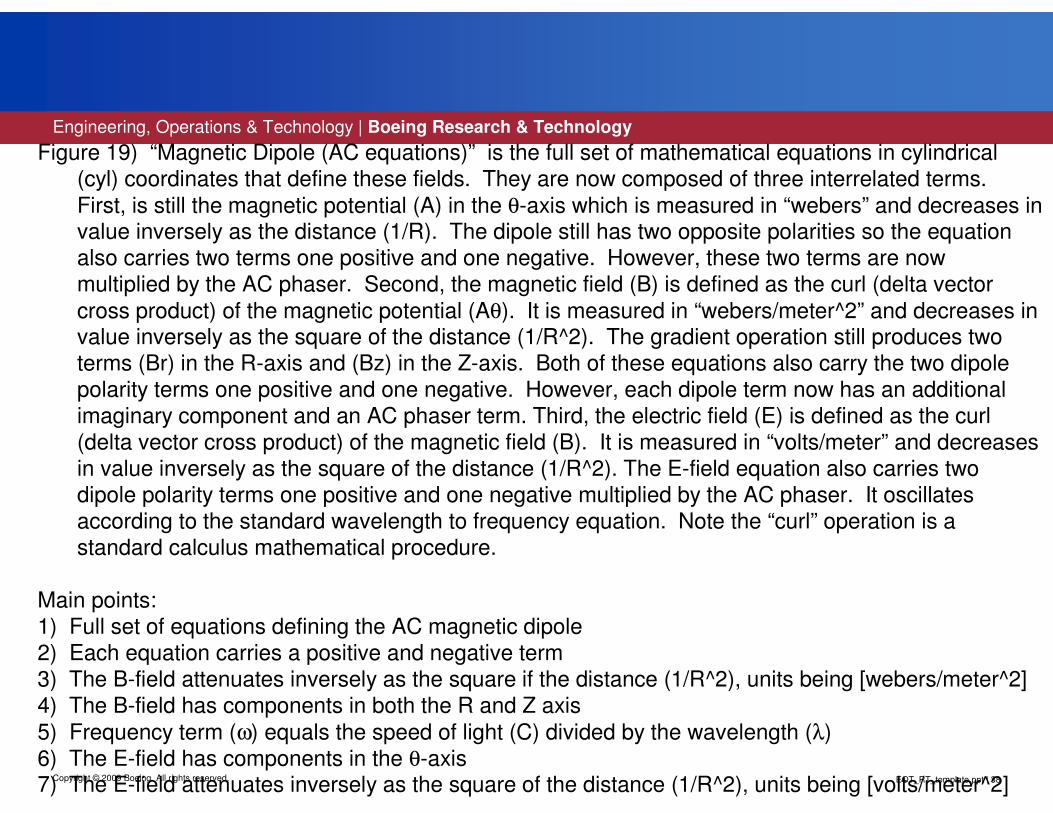
Figure 19) “Magnetic Dipole (AC equations)” is the full set of mathematical equations in cylindrical (cyl) coordinates that define these fields. They are now composed of three interrelated terms.
First, is still the magnetic potential (A) in the θ-axis which is measured in “webers” and decreases in value inversely as the distance (1/R). The dipole still has two opposite polarities so the equation also carries two terms one positive and one negative. However, these two terms are now multiplied by the AC phaser. Second, the magnetic field (B) is defined as the curl (delta vector
cross product) of the magnetic potential (Aθ). It is measured in “webers/meter^2” and decreases in value inversely as the square of the distance (1/R^2). The gradient operation still produces two terms (Br) in the R-axis and (Bz) in the Z-axis. Both of these equations also carry the two dipole polarity terms one positive and one negative. However, each dipole term now has an additional imaginary component and an AC phaser term. Third, the electric field (E) is defined as the curl (delta vector cross product) of the magnetic field (B). It is measured in “volts/meter” and decreases in value inversely as the square of the distance (1/R^2). The E-field equation also carries two dipole polarity terms one positive and one negative multiplied by the AC phaser. It oscillates according to the standard wavelength to frequency equation. Note the “curl” operation is a standard calculus mathematical procedure.
Main points:1) Full set of equations defining the AC magnetic dipole2) Each equation carries a positive and negative term3) The B-field attenuates inversely as the square if the distance (1/R^2), units being [webers/meter^2]4) The B-field has components in both the R and Z axis
5) Frequency term (ω) equals the speed of light (C) divided by the wavelength (λ)6) The E-field has components in the θ-axis7) The E-field attenuates inversely as the square of the distance (1/R^2), units being [volts/meter^2]

EOT_RT_template.ppt | 39Copyright © 2009 Boeing. All rights reserved.
WAVE BASICS
Standing/Traveling
Mg10
Page 20

EOT_RT_template.ppt | 40
Engineering, Operations & Technology | Boeing Research & Technology
Copyright © 2009 Boeing. All rights reserved.
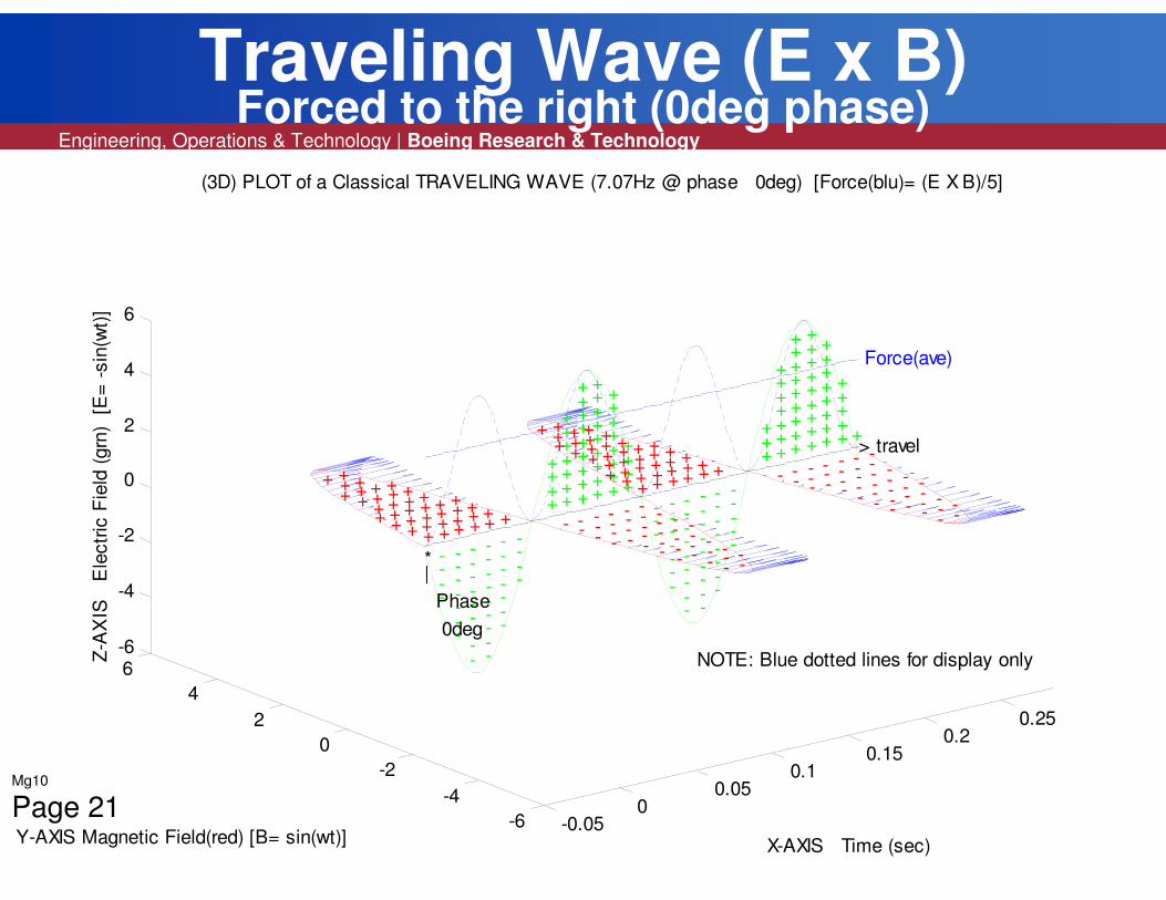
Figure 20) “Wave Basics (standing/traveling)” is a short tutorial on (EM)
ElectroMagnetic waves. The following figures are all textbook examples of EM waves with orthogonal (90deg) electric and magnetic fields. The electric field (E-
field) colored green is represented as a sine wave [E= -sin(ωt)] on the Z-axis with its polarity defined as (+) positive in the positive Z-axis (z= “+”). Likewise, the magnetic
field (B-field) colored red is represented as a sine wave [B= sin(ωt)] on the Y-axis with its polarity defined as (+) positive in the positive Y-axis (y= “+”). Each of the
following figures shows a different phase angle between these electric and magnetic
fields. This is background material for understanding the interactions between an
accelerating force field and the electric and magnetic fields.
EOT_RT_template.ppt | 41
Engineering, Operations & Technology | Boeing Research & Technology
Copyright © 2009 Boeing. All rights reserved.
DC and AC EM Dipoles
Traveling Wave (E x B)Forced to the right (0deg phase)
-0.050
0.050.1
0.150.2
0.25
-6
-4
-2
0
2
4
6-6
-4
-2
0
2
4
6
--
---
----
----
-----
------> travel
Force(ave)
-----
+
----
+++++
---
++++++++
---
+++++++++
--
+++++++++
-
+++++++
X-AXIS Time (sec)
+++
--
-----
---
--------
+
---
---------
++
NOTE: Blue dotted lines for display only
----
---------
+++
-----
-------
++++
--------
+++++
-----+++++
----
+++++++++
----
+++++++++++
(3D) PLOT of a Classical TRAVELING WAVE (7.07Hz @ phase 0deg) [Force(blu)= (E X B)/5]
++
---
+++++++++
++++
--
+++++++++
+++
-
+++++++
+++
++++
+
----
-------
+
---------
++
---------
+++
-------
++++
----
++++
0deg
Phase
|*
+++++
+++++
+++++
++++
+++
Y-AXIS Magnetic Field(red) [B= sin(wt)]
++++
Z-A
XIS
E
lectr
ic F
ield
(grn
) [
E=
-sin
(wt)
]
Mg10
Page 21

EOT_RT_template.ppt | 42
Engineering, Operations & Technology | Boeing Research & Technology
Copyright © 2009 Boeing. All rights reserved.
Figure 21) “Traveling Wave (0deg phase)” this figure shows 0deg phasing between the E-field and B-field which means that when the B-field is at a positive
maximum value the E-field is at a negative maximum. The vector cross product of the E and B fields (F= E x B) generates a force field represented by the blue arrows in the positive X-axis direction causing the wave to travel to the right (x= “+”) as all the force vectors push that way. The additional blue dotted wave
representation of the force vectors is for display clarity only, it is not really
present. However, as can be seen from this “display only” wave the force field is also a sine wave with a positive DC offset (average value) and twice the
frequency (second harmonic) of the E and B fields. Thus the EM wave has two
force pulses per cycle pushing it forward.
Main points:
1) 0deg phase generates a wave traveling to the right
2) The resultant force field is also a sine wave at twice the frequency
3) This force field has an average DC value pushing it forward
EOT_RT_template.ppt | 43
Engineering, Operations & Technology | Boeing Research & Technology
Copyright © 2009 Boeing. All rights reserved.
DC and AC EM Dipoles
Standing Wave (E x B)Force = 0 (90deg phase)
-0.050
0.050.1
0.150.2
0.25
-6
-4
-2
0
2
4
6-6
-4
-2
0
2
4
6
-----
-----
---
----
-- Force(ave)=0
--
+
-
+++++
-
++++++++
+++++++++
-
+++++++++
--
++++++++
--
X-AXIS Time (sec)
-
+++++
----
+++
----
-----
+++
-----
--------
++++
-----
---------
++
NOTE: Blue dotted lines for display only
+++
-----
---------
++++++
----
-------
+++++
---
---
++++
--
++++
-
++++
+++
-
++++++++
(3D) PLOT of a Classical STANDING WAVE (7.07Hz @ phase 90deg) [Force(blu)= (E X B)/5]
++
+++++++++
-
+++++++++
--
++++++++
---
++++++
---
++
-------
+++
----
-------
++++
----
---------
+++++
|*
---
---------
++++++
--
-------
+++++
-
----
++++
90deg
Phase
|*
++++
++++
++
Y-AXIS Magnetic Field(red) [B= -cos(wt)]
Z-A
XIS
E
lectr
ic F
ield
(grn
) [
E=
-sin
(wt)
]
Mg10
Page 22
EOT_RT_template.ppt | 44
Engineering, Operations & Technology | Boeing Research & Technology
Copyright © 2009 Boeing. All rights reserved.
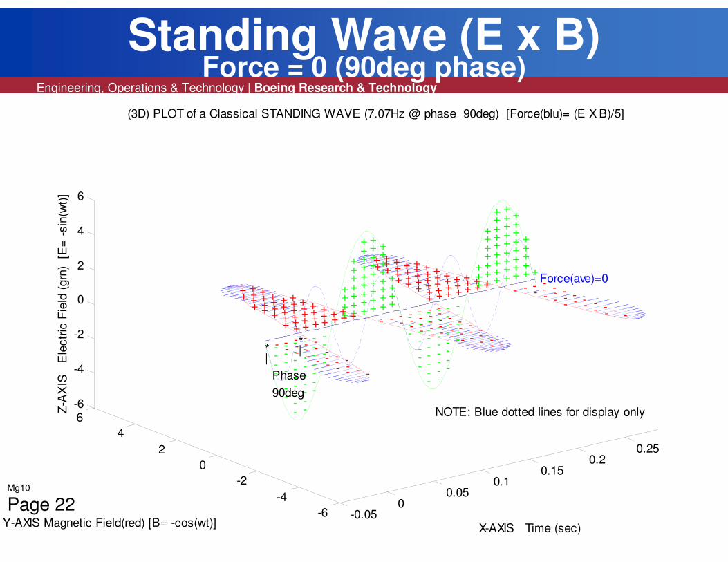
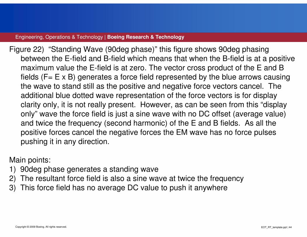
Figure 22) “Standing Wave (90deg phase)” this figure shows 90deg phasing
between the E-field and B-field which means that when the B-field is at a positive
maximum value the E-field is at zero. The vector cross product of the E and B fields (F= E x B) generates a force field represented by the blue arrows causing
the wave to stand still as the positive and negative force vectors cancel. The additional blue dotted wave representation of the force vectors is for display
clarity only, it is not really present. However, as can be seen from this “display
only” wave the force field is just a sine wave with no DC offset (average value)
and twice the frequency (second harmonic) of the E and B fields. As all the positive forces cancel the negative forces the EM wave has no force pulses
pushing it in any direction.
Main points:
1) 90deg phase generates a standing wave
2) The resultant force field is also a sine wave at twice the frequency
3) This force field has no average DC value to push it anywhere
EOT_RT_template.ppt | 45
Engineering, Operations & Technology | Boeing Research & Technology
Copyright © 2009 Boeing. All rights reserved.
Traveling Wave (E x B)Forced to the left (180deg phase)
-0.050
0.050.1
0.150.2
0.25
-6
-4
-2
0
2
4
6-6
-4
-2
0
2
4
6
Force(ave)
+
--
++++++
---
+++++++++
----
+++++++++++
----
++++++++++++
-----
+++++++++++
X-AXIS Time (sec)
-----
++++++++
-----+++++
----
-----
+++++
---
--------
+++++
---
---------
NOTE: Blue dotted lines for display only
++++
--
---------
+++
-
-------
+++
---
+
-
++++
---
+++++++++
(3D) PLOT of a Classical TRAVELING WAVE (7.07Hz @ phase 180deg) [Force(blu)= (E X B)/5]
---
+++++++++++
----
++++++++++++
-----
+++++++++++
-----
++++++++
-----|*
+++++
----
----
+++++
----
-------
+++++
---
---------
+++++
--
---------
+++
-
-------
+++
----
+
180deg
Phase
|*
travel <
Y-AXIS Magnetic Field(red) [B= -sin(wt)]
Z-A
XIS
E
lectr
ic F
ield
(grn
) [
E=
-sin
(wt)
]
Mg10
Page 23
EOT_RT_template.ppt | 46
Engineering, Operations & Technology | Boeing Research & Technology
Copyright © 2009 Boeing. All rights reserved.
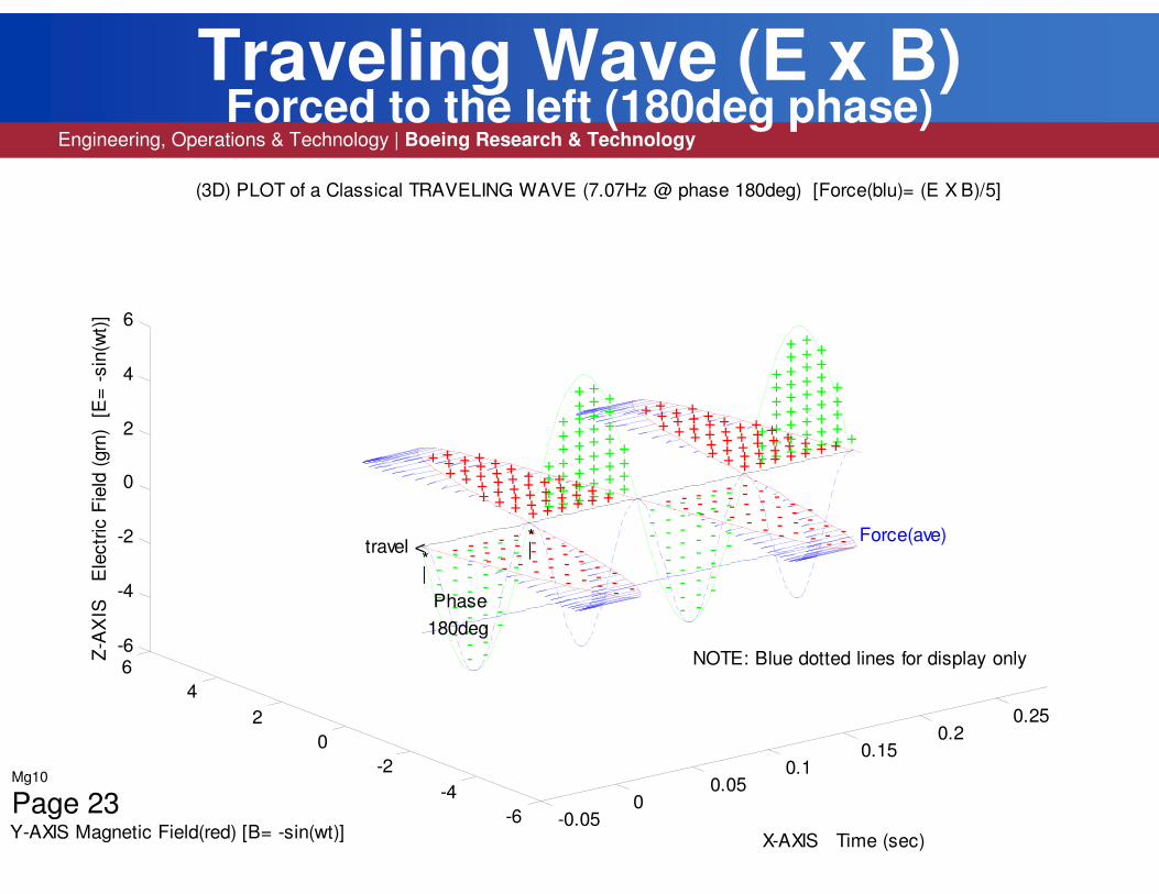
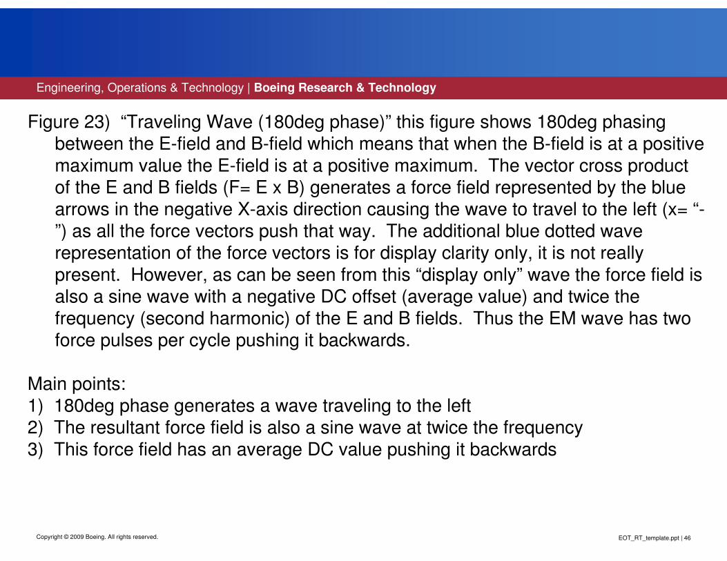
Figure 23) “Traveling Wave (180deg phase)” this figure shows 180deg phasing
between the E-field and B-field which means that when the B-field is at a positive
maximum value the E-field is at a positive maximum. The vector cross product of the E and B fields (F= E x B) generates a force field represented by the blue
arrows in the negative X-axis direction causing the wave to travel to the left (x= “-”) as all the force vectors push that way. The additional blue dotted wave
representation of the force vectors is for display clarity only, it is not really
present. However, as can be seen from this “display only” wave the force field is also a sine wave with a negative DC offset (average value) and twice the
frequency (second harmonic) of the E and B fields. Thus the EM wave has two
force pulses per cycle pushing it backwards.
Main points:
1) 180deg phase generates a wave traveling to the left
2) The resultant force field is also a sine wave at twice the frequency
3) This force field has an average DC value pushing it backwards

EOT_RT_template.ppt | 47
Engineering, Operations & Technology | Boeing Research & Technology
Copyright © 2009 Boeing. All rights reserved.
DC and AC EM Dipoles
Standing Wave (E x B)Force = 0 (270deg phase)
-0.050
0.050.1
0.150.2
0.25
-6
-4
-2
0
2
4
6-6
-4
-2
0
2
4
6
----
---
---
Force(ave)=0
-
+
-----
++++++
-----
++++++++++
-----
++++++++++++
-----
+++++++++++++
----
++++++++++
X-AXIS Time (sec)
---
+++
+++
--
+++
-
-----
++
-
--------
++
---------
NOTE: Blue dotted lines for display only
-
---------
--
-------
+
---
---
++
----
++
----
+++++++
-----
++++++++++++
(3D) PLOT of a Classical STANDING WAVE (7.07Hz @ phase 270deg) [Force(blu)= (E X B)/5]
------
++++++++++++++
-----|*
+++++++++++++++
----
+++++++++++
---
++++
++++
--
++++
--
----
+++
-
-------
++
---------
---------
-------
+
----
++
270deg
Phase
|*
++
+++
+++
++++
++
Y-AXIS Magnetic Field(red) [B= cos(wt)]
+++++
++++
Z-A
XIS
E
lectr
ic F
ield
(grn
) [
E=
-sin
(wt)
]
Mg10
Page 24
EOT_RT_template.ppt | 48
Engineering, Operations & Technology | Boeing Research & Technology
Copyright © 2009 Boeing. All rights reserved.
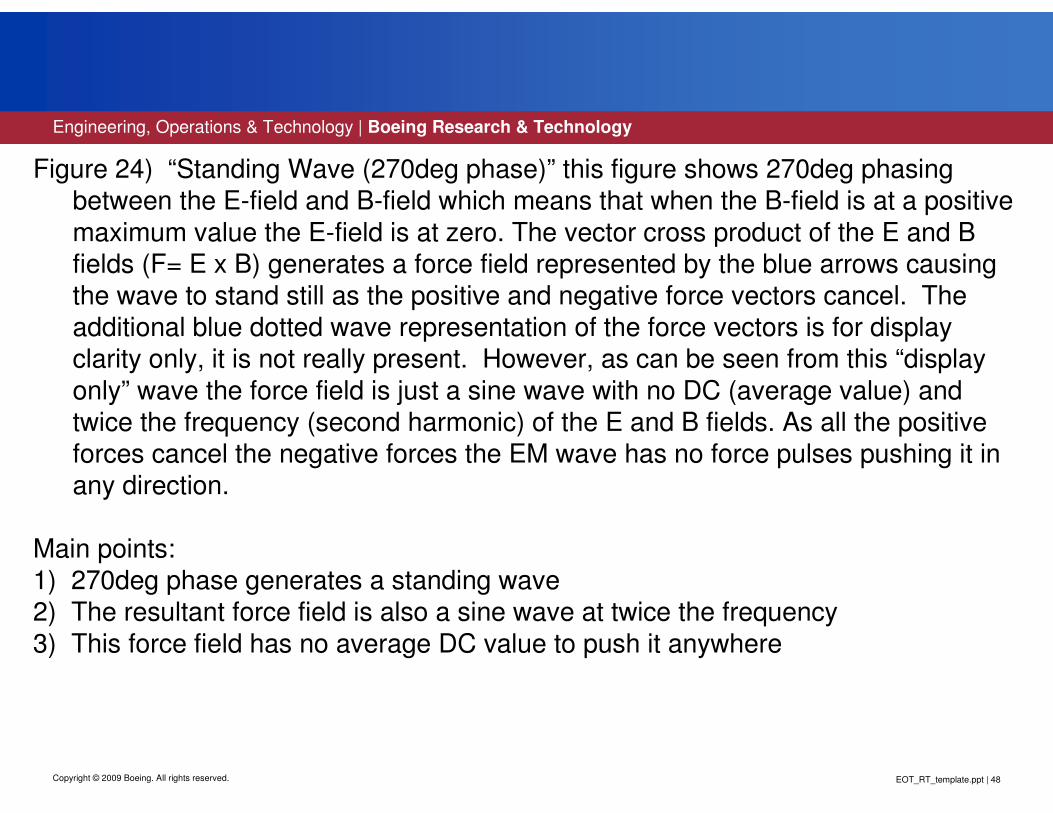
Figure 24) “Standing Wave (270deg phase)” this figure shows 270deg phasing
between the E-field and B-field which means that when the B-field is at a positive
maximum value the E-field is at zero. The vector cross product of the E and B fields (F= E x B) generates a force field represented by the blue arrows causing
the wave to stand still as the positive and negative force vectors cancel. The additional blue dotted wave representation of the force vectors is for display
clarity only, it is not really present. However, as can be seen from this “display
only” wave the force field is just a sine wave with no DC (average value) and
twice the frequency (second harmonic) of the E and B fields. As all the positive forces cancel the negative forces the EM wave has no force pulses pushing it in
any direction.
Main points:
1) 270deg phase generates a standing wave
2) The resultant force field is also a sine wave at twice the frequency
3) This force field has no average DC value to push it anywhere

EOT_RT_template.ppt | 49
Engineering, Operations & Technology | Boeing Research & Technology
Copyright © 2009 Boeing. All rights reserved.
E x B Wave Phasing
• E-field and B-field in phase (0deg)• F-field pushing wave to the right
• E-field and B-field out of phase (90deg)• Standing wave (F-field = 0)
• E-field and B-field out of phase (180deg)• F-field pushing wave to the left
• E-field and B-field out of phase (270deg)• Standing wave (F-field = 0)
• Two F-field pulses per cycle (traveling wave)• Fast acceleration• Frequency multiplication (doubling)
Mg10
Page 25
EOT_RT_template.ppt | 50
Engineering, Operations & Technology | Boeing Research & Technology
Copyright © 2009 Boeing. All rights reserved.
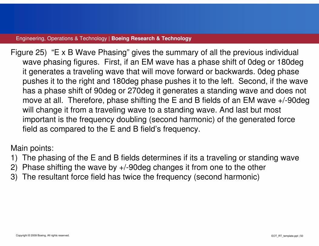
Figure 25) “E x B Wave Phasing” gives the summary of all the previous individual
wave phasing figures. First, if an EM wave has a phase shift of 0deg or 180deg it generates a traveling wave that will move forward or backwards. 0deg phase pushes it to the right and 180deg phase pushes it to the left. Second, if the wave
has a phase shift of 90deg or 270deg it generates a standing wave and does not move at all. Therefore, phase shifting the E and B fields of an EM wave +/-90deg
will change it from a traveling wave to a standing wave. And last but most
important is the frequency doubling (second harmonic) of the generated force
field as compared to the E and B field’s frequency.
Main points:
1) The phasing of the E and B fields determines if its a traveling or standing wave2) Phase shifting the wave by +/-90deg changes it from one to the other
3) The resultant force field has twice the frequency (second harmonic)

EOT_RT_template.ppt | 51Copyright © 2009 Boeing. All rights reserved.
Data from:
Study of Gravity (part 1)
Mg10
Page 26

EOT_RT_template.ppt | 52
Engineering, Operations & Technology | Boeing Research & Technology
Copyright © 2009 Boeing. All rights reserved.
Figure 26) “Data from: Study of Gravity (part 1)” Starting with these equations and
using the all the proceeding tutorials as background material the presentation continues toward the goal merging the earths accelerating force (gravity) field with (EM) ElectroMagnatics. However, the mathematics gets more complex as the EM field equations deal with calculus and imaginary numbers.
EOT_RT_template.ppt | 53
Engineering, Operations & Technology | Boeing Research & Technology
Copyright © 2009 Boeing. All rights reserved.
STUDY OF GRAVITY (Part 1)Errata List
• Misspelled the word lambda (not lamda)• Left (not right) Hand Motor rule• Acceleration field attenuation 1/R^2 or 1/R^3
(not 1/R)
Mg10
Page 27
EOT_RT_template.ppt | 54
Engineering, Operations & Technology | Boeing Research & Technology
Copyright © 2009 Boeing. All rights reserved.
Figure 27) “Study of Gravity (part 1) errata list” In the time this study has been out
in public domain three errors have been brought to my attention. First, miss-spelled
the word “Lambda” as lamda. Second, the motor rule is defined as the “left” hand and the generator rule is the “right” hand. And third, The attenuation of the
acceleration force field must be greater than linear (1/R) if it is connected with (EM) ElectroMagnetic fields as they attenuate as the square of the distance (1/R^2).

EOT_RT_template.ppt | 55
Engineering, Operations & Technology | Boeing Research & Technology
Copyright © 2009 Boeing. All rights reserved.
R-Axis Dipole PlotS (part 1) English to Metric conversion
0 1 2 3 4 5 6 7 8 9 10
x 104
-0.04
-0.035
-0.03
-0.025
-0.02
-0.015
-0.01
-0.005
0
0.005
0.01
Dis tance (Km)
Radia
l A
ccele
ration[p
k]
(Km
/sec2)
ATTENUATION (R-ax is) of RADIAL W AVES of ACCELERATION
*
< >Inner
Belt
*
<--- --->Outer
Belt
|< W ave Length (7.07Hz)
|< Geo Sync= 42091.7Km
|< Lambda= 42432.8Km |< 2Lambda= 84865.6Km
Acc(pk)= -0.01540Km/sec2 @ Earth Radius(1Re)= 6377.5Km
Dipole(A/B)= 4714.76Km
A-Field (1/R-blk)= -1.61e+001(1.0s in(7.07Hz) +1.5s in(14.14Hz) +1.2s in(21.21Hz) +1.1s in(28.28Hz)) [Km/sec2]
A -Field(1/R2-blu)= -6.40e+005(1.0s in(7.07Hz) +1.5s in(14.14Hz) +1.2s in(21.21Hz) +1.1s in(28.28Hz)) [Km/sec2]
A -Field(1/R3-red)= -2.40e+010(1.0s in(7.07Hz) +1.5s in(14.14Hz) +1.2s in(21.21Hz) +1.1s in(28.28Hz)) [Km/sec2]
A ll F ields : "+"= Radial Out "-"= Radial In
|
A/B
|
1Re
|
2Re
|
3Re
|
4Re
|
5Re
|
6Re
|
7Re
|
8Re
|
9Re
|
10Re
|
11Re
|
12Re
|
13Re
|
14Re
|< surface= -9.807m/sec2(ave)
*
Geo Sync=
|< 42091.5Km
*
Outer Edge of
Magnetosphere=
|< 84183.1Km
Mg10
Page 28
EOT_RT_template.ppt | 56
Engineering, Operations & Technology | Boeing Research & Technology
Copyright © 2009 Boeing. All rights reserved.
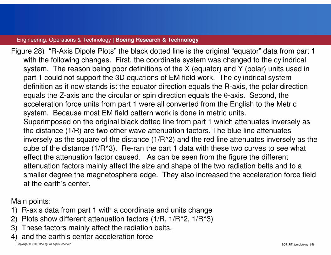
Figure 28) “R-Axis Dipole Plots” the black dotted line is the original “equator” data from part 1 with the following changes. First, the coordinate system was changed to the cylindrical
system. The reason being poor definitions of the X (equator) and Y (polar) units used in part 1 could not support the 3D equations of EM field work. The cylindrical system
definition as it now stands is: the equator direction equals the R-axis, the polar direction
equals the Z-axis and the circular or spin direction equals the θ-axis. Second, the acceleration force units from part 1 were all converted from the English to the Metric
system. Because most EM field pattern work is done in metric units. Superimposed on the original black dotted line from part 1 which attenuates inversely as
the distance (1/R) are two other wave attenuation factors. The blue line attenuates inversely as the square of the distance (1/R^2) and the red line attenuates inversely as the
cube of the distance (1/R^3). Re-ran the part 1 data with these two curves to see what effect the attenuation factor caused. As can be seen from the figure the different
attenuation factors mainly affect the size and shape of the two radiation belts and to a smaller degree the magnetosphere edge. They also increased the acceleration force field
at the earth’s center.
Main points:
1) R-axis data from part 1 with a coordinate and units change2) Plots show different attenuation factors (1/R, 1/R^2, 1/R^3)
3) These factors mainly affect the radiation belts, 4) and the earth’s center acceleration force

EOT_RT_template.ppt | 57
Engineering, Operations & Technology | Boeing Research & Technology
Copyright © 2009 Boeing. All rights reserved.
Z-Axis Dipole PlotS (part 1) English to Metric conversion
-1 -0.8 -0.6 -0.4 -0.2 0 0.2 0.4 0.6 0.8 1
x 105
-0.04
-0.035
-0.03
-0.025
-0.02
-0.015
-0.01
-0.005
0
0.005
0.01
Dis tance (Km)
Radia
l A
ccele
ration[p
k]
(Km
/sec2)
ATTENUATION (Z-ax is) of RADIAL W AVES of ACCELERATION
|<W ave Length (7.07Hz)
|< Geo Sync= 42091.7Km
|< Lambda= 42432.8Km |< 2Lambda= 84865.6Km
Acc(pk)= -0.01540Km/sec2 @ Earth Radius(1Re)= 6377.5Km
Dipole(A /B )= 4714.76Km
A-Field (1/R-blk )= -1.61e+001(1.0s in(7.07Hz) +1.5s in(14.14Hz) +1.2s in(21.21Hz) +1.1s in(28.28Hz)) [Km/sec2]
A-Field(1/R2-blu)= -6.40e+005(1.0s in(7.07Hz) +1.5s in(14.14Hz) +1.2s in(21.21Hz) +1.1s in(28.28Hz)) [Km/sec2]
A-Field(1/R3-red)= -2.40e+010(1.0s in(7.07Hz) +1.5s in(14.14Hz) +1.2s in(21.21Hz) +1.1s in(28.28Hz)) [Km/sec2]
A ll Fields: "+ "= Radial Out "-"= Radial In
| *
A
*
B
|
1Re
|
2Re
|
3Re
|
4Re
|
5Re
|
6Re
|
7Re
|
8Re
|
9Re
|
10Re
|
11Re
|
12Re
|
13Re
|
14Re
|< surface= -9.807m/sec2(ave)
*
Geo Sync=
|< 42091.5Km
*
Outer Edge of
Magnetosphere=
|< 84183.1Km
Mg10
Page 29

EOT_RT_template.ppt | 58
Engineering, Operations & Technology | Boeing Research & Technology
Copyright © 2009 Boeing. All rights reserved.
Figure 29) “Z-Axis Dipole Plots” similarly the black dotted line is the original ”polar”data from part 1 with the exact same changes that were preformed on the previous R-axis figure and for the same reasons (cylindrical coordinates, metric system).
Superimposed on the original black dotted line from part 1 which attenuates inversely as the distance (1/R) are the same two wave attenuation factors. The blue line attenuates inversely as the square of the distance (1/R^2) and the red
line attenuates inversely as the cube of the distance (1/R^3). Re-ran the part 1
data with these two curves to see what effect the attenuation factor caused. As can be seen from the figure the two different attenuation factors mainly affect the
size and shape of the area close to the poles that being the region of the “Aurora
Borealis” or as its more commonly called the northern and southern lights and to
a smaller degree the magnetosphere edge. They also increased the
acceleration force field at the earth’s center.
Main points:1) Z-axis data from part 1 with the same coordinate and unit changes
2) Plots show different attenuation factors (1/R, 1/R^2, 1/R^3)
3) These factors mainly affect the near earth region,
4) and the earth’s center acceleration force

EOT_RT_template.ppt | 59
Engineering, Operations & Technology | Boeing Research & Technology
Copyright © 2009 Boeing. All rights reserved.
PHYSICS: Poynting Vector
• Force Field Equation
• Starting with the Poynting Vector equation:
• P = (1/µµµµo)*E x B [watts/m^2]
• Removing the 1/µµµµo term reduces theE x B units [watts/m^2] to [newton-ohms/m^2]
• Free space resistance: Rs = (µµµµo/εεεεo)^.5 [ohms]• Multiplying E x B by the reciprocal of resistance [1/Rs]
produces the free space force field equation:
• F = (εεεεo/µµµµo)^.5*E x B [newton/m^2]
Mg10
Page 30

EOT_RT_template.ppt | 60
Engineering, Operations & Technology | Boeing Research & Technology
Copyright © 2009 Boeing. All rights reserved.
Figure 30) “Physics: Poynting Vector” Straight from the textbook states that Power
density (P) of an EM wave is equal to the vector cross product of the E and B
fields divided by the magnetic permeability (µµµµo) of free space, units being [watts/meter^2]. One method of deriving the force field equation (F= E x B) is to
modify the Poynting vector equation as force, work and power are all closely related (change of constants). First, removing the magnetic permeability
constant (1/µµµµo) reduces the equation’s units from [watts/meter^2] to [newton-ohms/meter^2]. Second, free space resistance (Rs) is equal to the square root of
the magnetic permeability (µµµµo) divided by the electric permittivity (εεεεo) expressed in [ohms]. Third, multiplying the equation by the reciprocal of the free space
resistance [1/Rs] produces the force field equation with the correct constants,
units being [newtons/meter^2].
Main points:
1) Textbook Poynting vector equation, units being [watts/meter^2] 2) Power and force are related terms, 3) need only to change the constants to get force, units being [newtons/meter^2]
EOT_RT_template.ppt | 61
Engineering, Operations & Technology | Boeing Research & Technology
Copyright © 2009 Boeing. All rights reserved.
PHYSICS: Left Hand Motor Rule
Force equals [L] length times [I] current “vector cross product” Magnetic [B] field
• Ohms Law: I = V / R• Where V = E[volts/meter] * L [meters]
• Boundary conditions apply:• Field constrained in a conductor (i.e. wire)• Length (L) of conductor in B-field• Resistance (R) of conductor
• F = (L^2/R)*E X B [newtons]
F = L*I X B
Mg10
Page 31

EOT_RT_template.ppt | 62
Engineering, Operations & Technology | Boeing Research & Technology
Copyright © 2009 Boeing. All rights reserved.
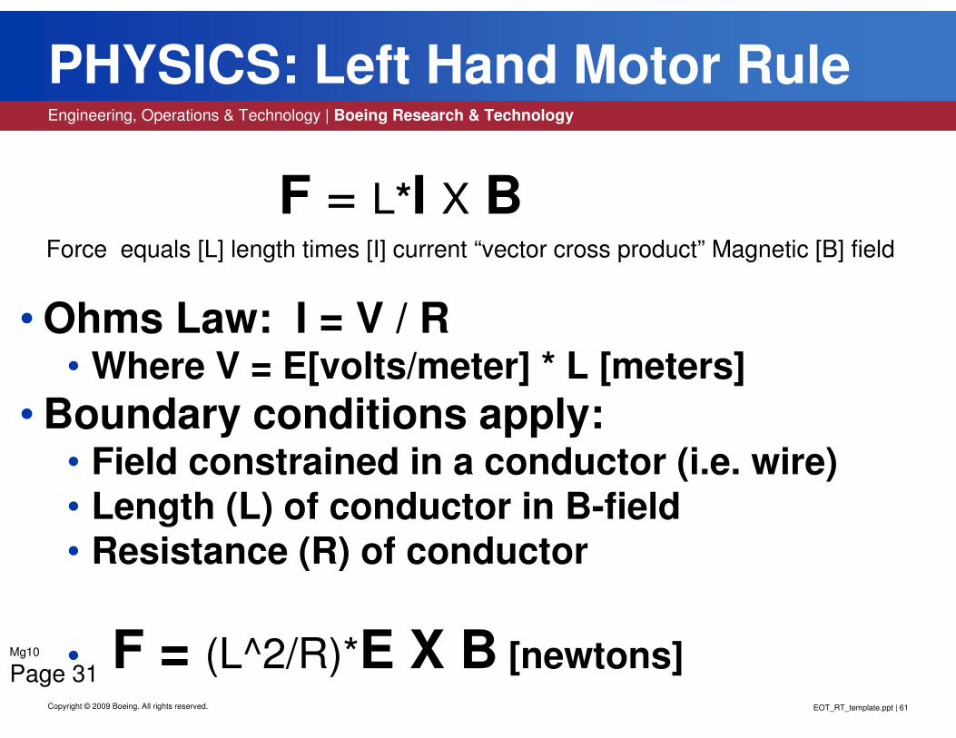
Figure 31) “Physics: Left Hand Motor Rule” or as it’s more commonly known the
Lorentz force equation (F = L*I x B) which states that Force is equal the Length of a conductor in a magnetic (B) field multiplied by the current (I) flowing through it. The vector cross product makes all three terms orthogonal (90deg). This is
another method of deriving the force equation. Remembering ohms law which states that current (I) is equal to the Voltage divided by the Resistance (voltage and current in phase). Making this substitution Force is now equal to the
conductor Length in the magnetic (B) field multiplied by the Voltage across it
and divided by the conductor Resistance. In a conductor the Voltage is equal to the integral of the Electric field over (multiply) the Length of the conductor.
Making this last substitution Force is now equal to the square of conductor
Length in the magnetic (B) field multiplied by the Electric field around it and divided by the conductor Resistance, units being [newtons].
Main points:1) Textbook Lorentz force equation, units being [newtons]2) Equation modified with ohm’s law substitution
3) Boundary conditions apply (not free space),
4) These changes correctly balance the force equation
EOT_RT_template.ppt | 63
Engineering, Operations & Technology | Boeing Research & Technology
Copyright © 2009 Boeing. All rights reserved.
Force Vector Product(cylindrical coordinates)
F = E x B = (EθθθθBz-EzBθθθθ) r + (EzBr-ErBz) θθθθ + (ErBθθθθ-EθθθθBr) z
F = (εo/µo)^.5[-(EzBθθθθ) r + (ErBθθθθ) z] Eθθθθ = Br = Bz = 0
F = (εo/µo)^.5[ (EθθθθBz) r - (EθθθθBr) z] Er = Ez = Bθθθθ = 0
Two possibilities either the B-field or E-field is in the theta direction.
Mg10
Page 32

EOT_RT_template.ppt | 64
Engineering, Operations & Technology | Boeing Research & Technology
Copyright © 2009 Boeing. All rights reserved.
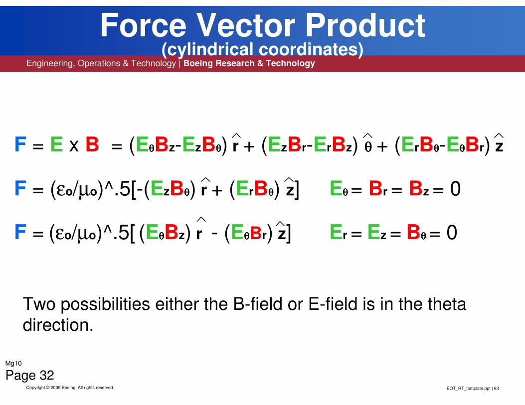
Figure 32) “Force Vector Product (cyl)” is the full blown mathematical vector cross
product for force in cylindrical coordinates. As can be seen it has four terms in each orthogonal axis. Also, each of the individual E and B fields have multiple
terms along with imaginary numbers so the complete equation gets very
complex to number crunch. However, the equation does have two general solutions depending on the boundary conditions used. Both solutions put the Force vector components in the R and Z axis but differ as to which EM field E or
B is in the circular θ-axis. First cut solution is to put the B-field in the R and Z axis as this is the normal position of the earth’s magnetic field in cylindrical coordinates.
Main points:
1) Complete force vector equation in cylindrical coordinates
2) The solution is complex as it has many terms some being imaginary
3) Only two general solutions possible, E or B field in the θ-axis
EOT_RT_template.ppt | 65
Engineering, Operations & Technology | Boeing Research & Technology
Copyright © 2009 Boeing. All rights reserved.
Wave Mixing
When two waves are mixed (multiplied) the output is the original frequencies (doubled) plus the sum and difference frequencies
B= -B0 -B1cos(θ) -B2cos(2θ)E= E2sin(2θ)F= E x B
(diff) (θθθθ doubled) (sum) (2θθθθ doubled)
F= -F1sin(2θ-θ) -F2sin(2θ) -F3sin(2θ+θ) -F4sin(4θ)
Mg10
Page 33
EOT_RT_template.ppt | 66
Engineering, Operations & Technology | Boeing Research & Technology
Copyright © 2009 Boeing. All rights reserved.
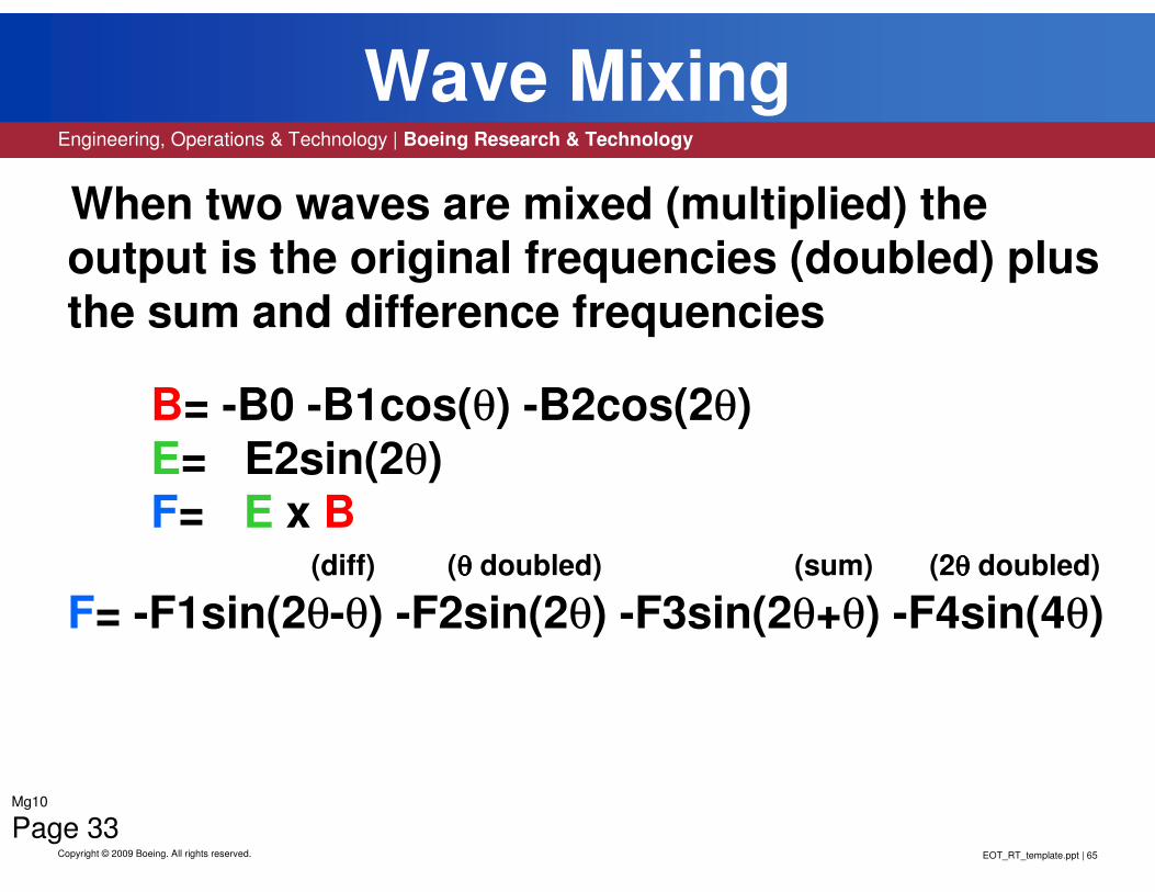
Figure 33) “Wave Mixing” shows the results of mixing (multiplying) two waves. The
first wave the B-field is composed of a fundamental [B1*cos(θ)] and second
harmonic [B2*cos(2θ)] along with a constant [B0], all terms being negative. The second wave the E-field is composed of only a fundamental [E2*sin(2θ)] which is the second harmonic of the B-field. Note the 90deg phase shift between the two waves (cosine vs sine). Multiplying (vector cross product) these two wave together results in a wave the F-field with four terms, all negative sines. This
mathematically shows the frequency doubling and phasing of the sum/difference
products of beat frequencies (mixing). This equation supports the “Wave Basics (stand/traveling)” tutorial showing that the accelerating force has twice the
frequency as its (EM) ElectroMagnetic components (two pulses per cycle). Also,
not shown is the correlation of the F-field constants: F1= E2*B1/2, F2= E2*B0, F3= E2*B1/2, F4= E2*B2.
Main points:
1) Wave mixing doubles the original frequencies
2) and generates sums and difference frequencies3) Mathematical proof that the force field operates on the second harmonic of the E
and B fields
4) Equates the four force field constant terms to the E and B field constants
EOT_RT_template.ppt | 67
Engineering, Operations & Technology | Boeing Research & Technology
Copyright © 2009 Boeing. All rights reserved.
Equator F = E x B Vectors
Mg10
Page 340 1 2 3 4 5 6 7 8 9 10
x 104
-0.04
-0.035
-0.03
-0.025
-0.02
-0.015
-0.01
-0.005
0
0.005
0.01
Distance (Km)
Radia
l A
ccele
ration[p
k]
(Km
/sec2)
RADIAL WAVES (R-axis) of ACCELERATION
*
< >Inner Belt
*
<--- --->Outer Belt
|< Wave Length (7.07Hz)|< Geo Sync= 42091.7Km|< Lambda= 42424.4Km |< 2Lambda= 84848.8Km
Acc(pk)= -0.01540Km/sec2 B-Field(dc)= 6.012e-005web/m2 @ Earth Radius(1Re)= 6377.5KmDipole(A/B)= 10606.10Km Bre-Field(ac)= 2.382e-005web/m2 Ere-Field(ac)= 3.699e-001volts/mB-Field(red)= -uo*(1.196e+015 -5.980e+014cos(7.07Hz) -5.980e+014cos(14.14Hz)) [web/m2]E-Field(grn)= 1.005e+010sin(14.14Hz) [volts/m]F-Field(blu)= -1.00e+013sin(7.07Hz)-1.50e+013sin(14.14Hz)-1.00e+013sin(21.21Hz)-1.10e+013sin(28.29Hz) [nt/Km2]A-Field(blk)= -1.00e+010sin(7.07Hz)-1.50e+010sin(14.14Hz)-1.20e+010sin(21.21Hz)-1.10e+010sin(28.29Hz) [Km/sec2]
|A/B
All Fields: "+"= Radial Out "-"= Radial In
| 1Re
| 2Re
| 3Re
| 4Re
| 5Re
| 6Re
| 7Re
| 8Re
| 9Re
|10Re
|11Re
|12Re
|13Re
|14Re
|< surface= -9.807m/sec2(ave)
*
Geo Sync=|< 42091.5Km
*
Outer Edge of Magnetosphere=
|< 84183.1Km*
Geo Sync=|< 42091.5Km
*
Outer Edge of Magnetosphere=
|< 84183.1Km
Mg10
Page 34

EOT_RT_template.ppt | 68
Engineering, Operations & Technology | Boeing Research & Technology
Copyright © 2009 Boeing. All rights reserved.
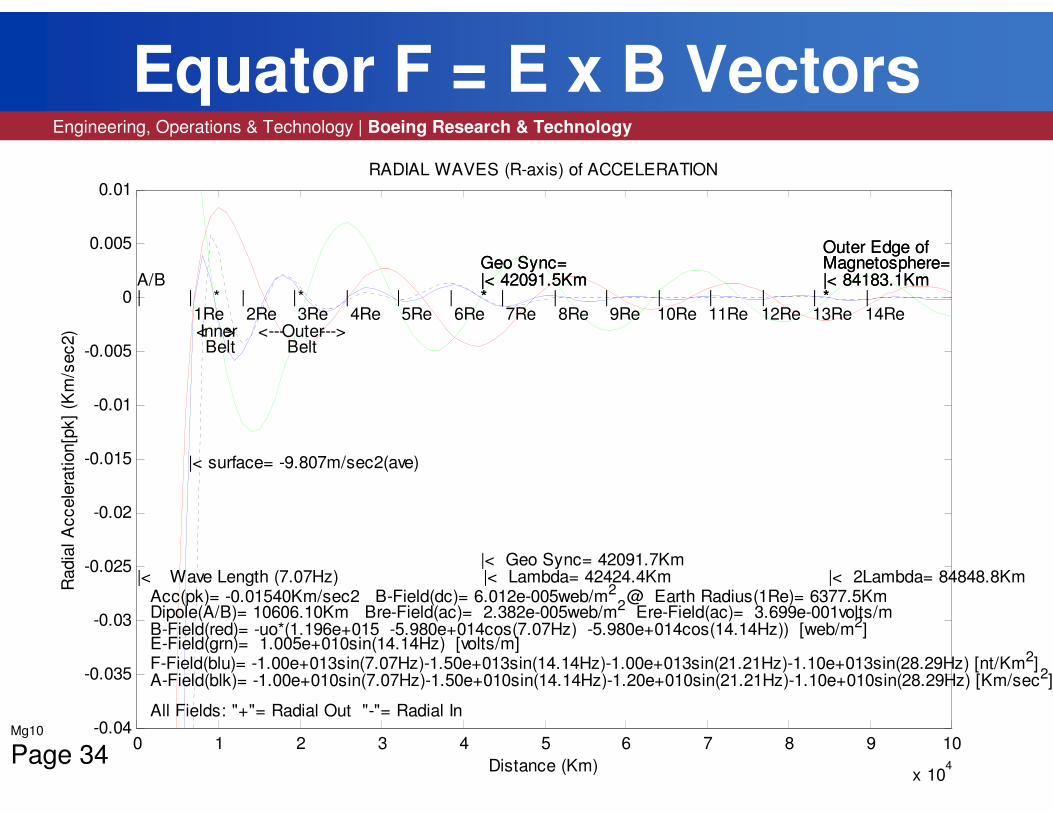
Figure 34) “Equator F = E x B Vectors” this figure is important as it shows the complete set of “Gravity” waves in the radial direction. The displayed equations are the simplified ones mainly to show the constants, but all the computations were done with the complete complex set. The Acceleration A-field[blk] is the original equation from part1 with the same relative term constants of A1= 1.0, A2= 1.5, A3= 1.2 and A4= 1.1. However, there are three modifications: first the coordinate system was changed to cylindrical, second the units were changed to metric and third the attenuation factor was changed to the inverse of the square of the distance (1/R^2). The Force F-field[blu] tracks or generates the proposed A-field almost exactly with very similar relative constants of F1= 1.0, F2= 1.5, F3= 1.0 and F4= 1.1. The third harmonic is a little lower which moved the inner radiation belt back to its correct position. As can be seen from the figure at distances less then the surface radius (Re) the (DC) Magnetic B-field[red] tracks the Force F-field[blu] however, at distances greater then the surface radius (Re) it starts oscillating (AC). The same is true for the Electric E-field[grn] only its phasing is different. In looking at the equation constants they all have numbers to high powers which generate very strong fields at the earth’s center (R= 0), but attenuate rapidly in the 3963 miles to the surface (R= Re) going down to uWebers for the Magnetic B-field and mVolts for the Electric E-field.
Main points:1) Plots the complete set of gravity waves2) Calculations run with the complex equations3) Attenuation factor is 1/R^2 4) High forces at the earth’s center (R= 0)5) and low forces at the surface (R= Re)6) Force field closely tracks the acceleration field7) Corrects the inner belt location
EOT_RT_template.ppt | 69
Engineering, Operations & Technology | Boeing Research & Technology
Copyright © 2009 Boeing. All rights reserved.
FFT Acceleration of Gravity (part 1)
0 5 10 15 20 25 30 35 400
0.5
1
1.5
2
2.5
3
3.5
4x 10
21
Frequency (Hz)
Rela
tive P
ow
er
(Acc2/H
z)
Acceleration Frequency Domain (FFT)
Calculated= 1.00 (7.03Hz) 2.15 (14.06Hz) 1.30 (21.09Hz) 1.15 (28.13Hz) +/-0.59Hz
NOTE: Due to Lambda/2 resonance the A2 term has a gain of "1.333" - (1.5 to 2.0)
Acceleration= 1.00e+010 (7.07Hz) 1.50e+010 (14.14Hz) 1.20e+010 (21.21Hz) 1.10e+010 (28.29Hz)
Mg10
Page 35

EOT_RT_template.ppt | 70
Engineering, Operations & Technology | Boeing Research & Technology
Copyright © 2009 Boeing. All rights reserved.
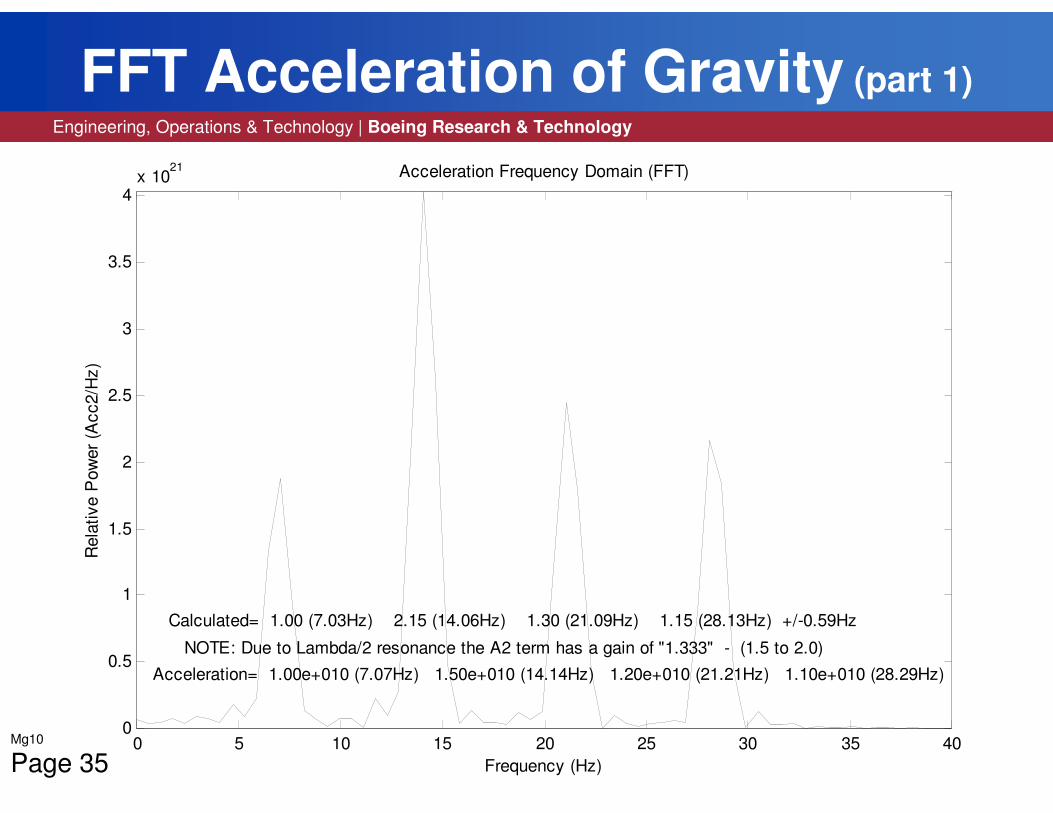
Figure 35) “FFT Acceleration of Gravity (part1)” shows the acceleration data from figure 34 only now in the frequency domain. It is composed of the same four
harmonics emphasizing their relative amplitudes. As can be seen by comparing
the Acc and Calc equations their constants are about the same except for the second harmonic. The second harmonic shows a resonant gain (2.15 vs 1.5) as
the dipole is tuned to this frequency. Dipole length is λ/2 at the second harmonic
or λ/4 at the fundamental frequency.
Main points:1) Four harmonics: (7.07Hz, 14.14Hz, 21.21Hz, 28.28Hz)
2) Relative constants: (1, 1.5, 1.2, 1.1)
3) The dipole is tuned to the second harmonic4) causing resonate gain at this frequency

EOT_RT_template.ppt | 71
Engineering, Operations & Technology | Boeing Research & Technology
Copyright © 2009 Boeing. All rights reserved.
FFT Gravity Force Field
0 5 10 15 20 25 30 35 400
0.5
1
1.5
2
2.5
3
3.5
4
x 1027
Frequency (Hz)
Rela
tive P
ow
er
(Forc
e2/H
z)
Force Frequency Domain (FFT)
Calculated= 1.00 (7.03Hz) 2.17 (14.06Hz) 0.89 (28.13Hz) 1.18 (35.16Hz) +/-0.59Hz
NOTE: Due to Lambda/2 resonance the F2 term has a gain of "1.333" - (1.5 to 2.0)
Force= 1.00e+013 (7.07Hz) 1.50e+013 (14.14Hz) 1.00e+013 (21.21Hz) 1.10e+013 (28.29Hz)
Mg10
Page 36
EOT_RT_template.ppt | 72
Engineering, Operations & Technology | Boeing Research & Technology
Copyright © 2009 Boeing. All rights reserved.
Figure 36) “FFT Gravity Force Field” shows the force data from figure 34 only now
in the frequency domain. It is composed of the same four harmonics
emphasizing their relative amplitudes. As can be seen by comparing the Acc and Calc equations their constants are about the same except for the second
harmonic. The second harmonic shows a resonant gain (2.17 vs 1.5) as the dipole is tuned to this frequency. The only difference between the previous
acceleration figure and this force one is the amplitude of the third harmonic and
the units.
Main points:
1) Same four harmonics: (7.07Hz, 14.14Hz, 21.21Hz, 28.28Hz)
2) Relative constants: (1, 1.5, 1.0, 1.1)3) The dipole is tuned to the second harmonic
4) causing resonate gain at this frequency
5) Difference in third harmonic amplitude (Acc vs Force)

EOT_RT_template.ppt | 73
Engineering, Operations & Technology | Boeing Research & Technology
Copyright © 2009 Boeing. All rights reserved.
Complete EM Dipole Br-Field Equation
• Br0 = µµµµoB0rz 2 / (r^2+z^2)^2 [dc term]
• Br1 = µµµµoB1rz[3 / (r^2+z^2)^2 [first harmonic]+i2ππππ / λλλλ(r^2+z^2)^1.5–i3λλλλ / 2ππππ(r^2+z^2)^2.5]exp(-iθθθθ)
• Br2 = µµµµoB1rz[3 / (r^2+z^2)^2 [second harmonic]+i4ππππ / λλλλ(r^2+z^2)^1.5–i3λλλλ / 4ππππ(r^2+z^2)^2.5]exp(-i2θθθθ)
• Br = Br0 +Br1 +Br2 [total]
Mg10
Page 37
EOT_RT_template.ppt | 74
Engineering, Operations & Technology | Boeing Research & Technology
Copyright © 2009 Boeing. All rights reserved.
Figure 37) “Complete EM Dipole Br-Field Equation” in cylindrical coordinates, it is composed of three terms a constant (DC) and two (AC) harmonics. The real
part (far field pattern) of all three terms attenuates inversely as the square of the
distance (1/D^2). Both harmonics also carry two complex (imaginary) terms (near field pattern) which attenuate inversely as the third (1/D^3) and fifth (1/D^5) powers of the distance respectively. Their effect is mainly at small
distances (< λ/2) which is where the planet and radiation belts are located sothey must be included in the calculations. The relative ratio of the coefficients:
B0 is equal to double (2x) B1.
Main points:
1) B-field in the R-axis is composed of three terms: a constant and the first and second harmonics
2) The far field pattern (real) attenuates (1/R^2), effects more at distances greater
than λ/23) The near field pattern (imaginary) attenuates faster (1/R^3, 1/R^5), effects more
at distances less than λ/24) Relative ratio of B-field constants: B0= 2*B1
EOT_RT_template.ppt | 75
Engineering, Operations & Technology | Boeing Research & Technology
Copyright © 2009 Boeing. All rights reserved.
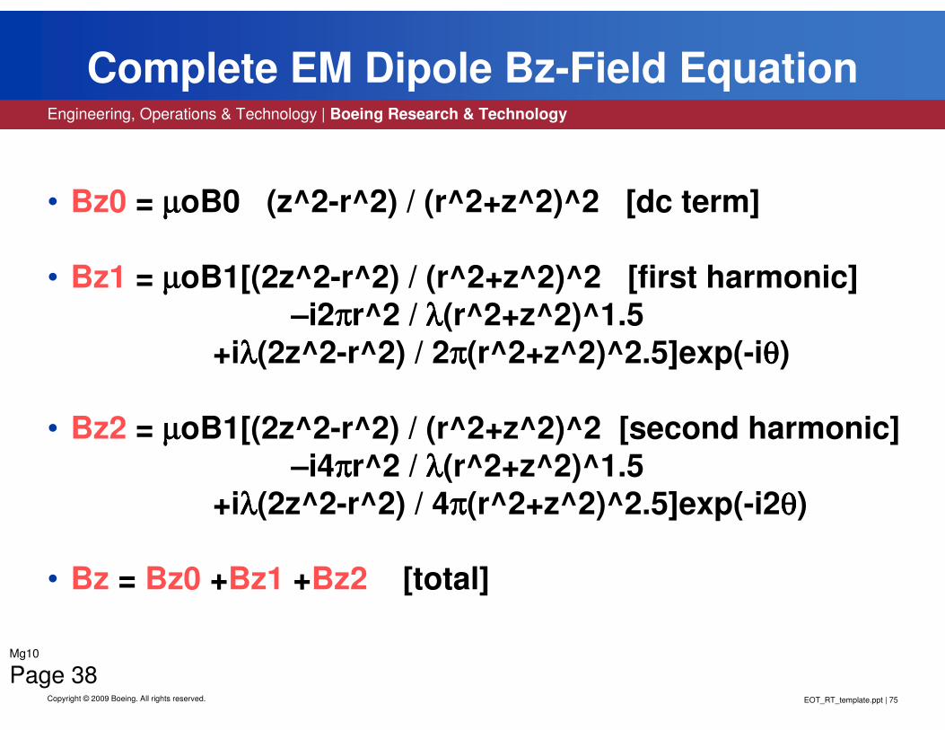
Complete EM Dipole Bz-Field Equation
• Bz0 = µµµµoB0 (z^2-r^2) / (r^2+z^2)^2 [dc term]
• Bz1 = µµµµoB1[(2z^2-r^2) / (r^2+z^2)^2 [first harmonic]–i2ππππr^2 / λλλλ(r^2+z^2)^1.5
+iλλλλ(2z^2-r^2) / 2ππππ(r^2+z^2)^2.5]exp(-iθθθθ)
• Bz2 = µµµµoB1[(2z^2-r^2) / (r^2+z^2)^2 [second harmonic]–i4ππππr^2 / λλλλ(r^2+z^2)^1.5
+iλλλλ(2z^2-r^2) / 4ππππ(r^2+z^2)^2.5]exp(-i2θθθθ)
• Bz = Bz0 +Bz1 +Bz2 [total]
Mg10
Page 38
EOT_RT_template.ppt | 76
Engineering, Operations & Technology | Boeing Research & Technology
Copyright © 2009 Boeing. All rights reserved.
Figure 38) “Complete EM Dipole Bz-Field Equation” in cylindrical coordinates, it is
also composed of three terms a constant (DC) and two (AC) harmonics.
Likewise the real part (far field pattern) of all three terms attenuates inversely as the square of the distance (1/D^2). Both harmonics also carry two similar
complex (imaginary) terms (near field pattern) which attenuate inversely as the third (1/D^3) and fifth (1/D^5) powers of the distance respectively. Their effect is
mainly at small distances (< λ/2) which is where the planet and radiation belts are located so they must be included in the calculations. The ratio of the coefficients is also B0 is equal to double (2x) B1.
Main points:
1) B-field in the Z-axis is also composed of three terms: a constant and the first and second harmonics
2) The far field pattern (real) attenuates (1/R^2), effects more at distances greater
than λ/23) The near field pattern (imaginary) attenuates faster (1/R^3, 1/R^5), effects more
at distances less than λ/24) Relative ratio of B-field constants: B0= 2*B1
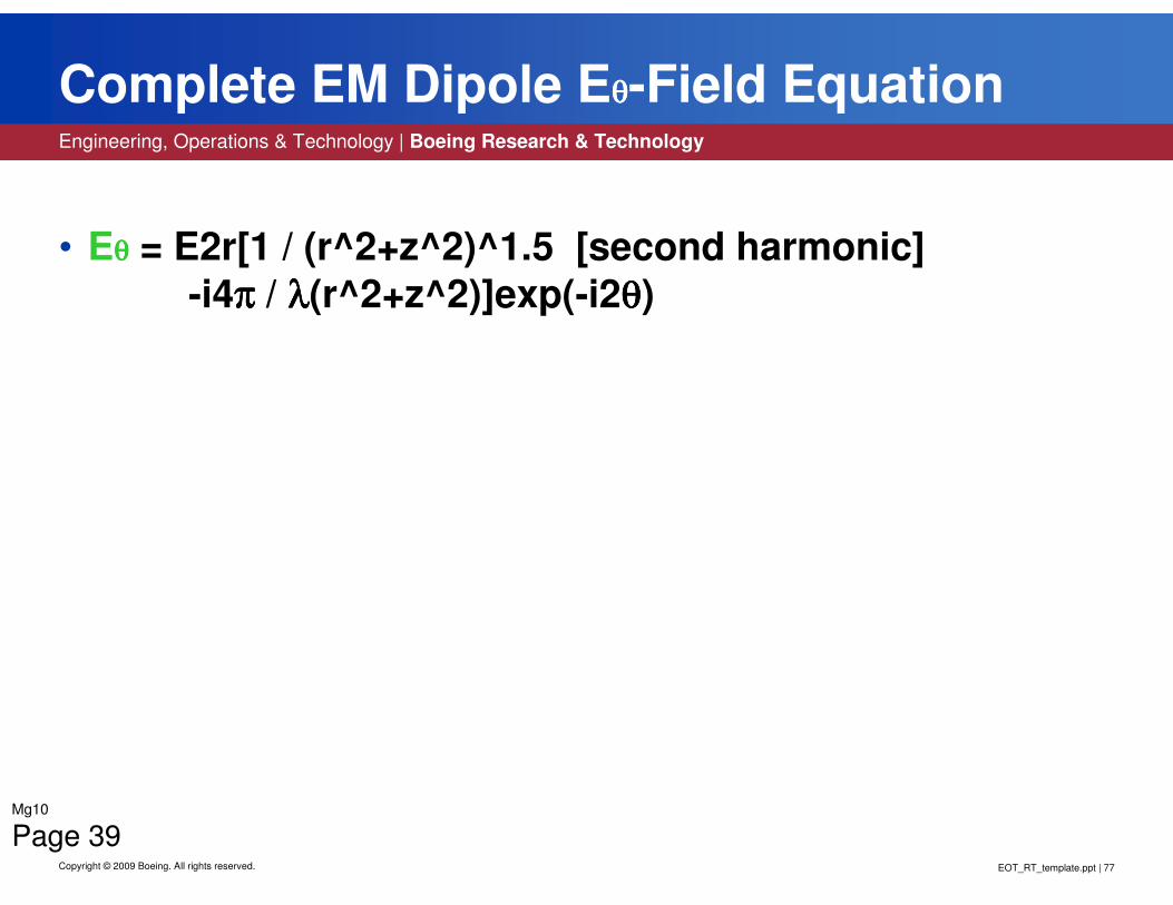
EOT_RT_template.ppt | 77
Engineering, Operations & Technology | Boeing Research & Technology
Copyright © 2009 Boeing. All rights reserved.
Complete EM Dipole Eθθθθ-Field Equation
• Eθθθθ = E2r[1 / (r^2+z^2)^1.5 [second harmonic]
-i4ππππ / λλλλ(r^2+z^2)]exp(-i2θθθθ)
Mg10
Page 39
EOT_RT_template.ppt | 78
Engineering, Operations & Technology | Boeing Research & Technology
Copyright © 2009 Boeing. All rights reserved.
Figure 39) “Complete EM Dipole Eθ-Field Equation” in cylindrical coordinates, it is composed of only the second (AC) harmonic term. There are no constant (DC) or first harmonic term. The real part (far field pattern) attenuates inversely as the
square of the distance (1/D^2). This harmonic also carries a complex (imaginary) term (near field pattern) which attenuates inversely as the cube
(1/D^3) of the distance. Its effect is mainly at small distances (< λ/2) which is where the planet and radiation belts are located so it must be included in the
calculations.
Main points:
1) E-field in the θ-axis is composed of only one term: the second harmonic2) The far field pattern (real) attenuates (1/R^2), effects more at distances greater
than λ/23) The near field pattern (imaginary) attenuates faster (1/R^3), effects more at
distances less than λ/2

EOT_RT_template.ppt | 79
Engineering, Operations & Technology | Boeing Research & Technology
Copyright © 2009 Boeing. All rights reserved.
Gravity F = E x B Vectors
EM Equations (simplified)
• B = -uo 6e14 (2 +1cos(θθθθ) +1cos(2θθθθ)) / (r^2+z^2)^1.5 [web/m^2]
• E = 1e10 sin(2θθθθ) / (r^2+z^2)^1.5 [volts/m]
• F = -1e13 (1.0sin(θθθθ) +1.5sin(2θθθθ) +1.0sin(3θθθθ) +1.1sin(4θθθθ)) / (r^2+z^2)^1.5 [nt/Km^2]
• A = -1e10 (1.0sin(θθθθ) +1.5sin(2θθθθ) +1.2sin(3θθθθ) +1.1sin(4θθθθ)) / (r^2+z^2)^1.5 [Km/s^2]
• F = M A
• Constant: M = [Kg/Km^2] ???<field mass density>???
Mg10
Page 40

EOT_RT_template.ppt | 80
Engineering, Operations & Technology | Boeing Research & Technology
Copyright © 2009 Boeing. All rights reserved.
Figure 40) “Gravity F = E x B Vectors” shows the simplified versions of the previous complex E[grn] and B[red] field equations along with the resultant force F-field[blu] from all the wave mixing (vector cross product). As can be seen by the equations and previous figures the Force field[blu] tracks the original Acceleration field[blk] almost exactly. However, there are three differences. First, there is a small change in relative value of the third harmonic coefficient from 1.2 to 1.0. Second, there is a change to the power of the constant term from 1E10 to 1E13. And third, is a difference in units nt/Km^2 vs Km/S^2. According to Newton’s law (F= M*A) Force and Acceleration are equivalent with Mass being the constant of proportionality, in theory this equation should also work with fields. Rearranging the equation and reducing the units, shows the Mass term to have units of [Kg/Km^2]. Reducing it further to [grams/meter^2] gives mass per area or some type of field density. The mass term could equal to the total earth mass and the area term equal the total earth surface area or it might be some kind of circular shaped integrating element where the fields combine. This is the one loose end in the entire “Study of Gravity”.
Main points:1) Simplified terms highlighting the equation constants and attenuation factor2) The force and acceleration equations almost identical3) One loose end, mass term units [Kg/Km^2] and definition
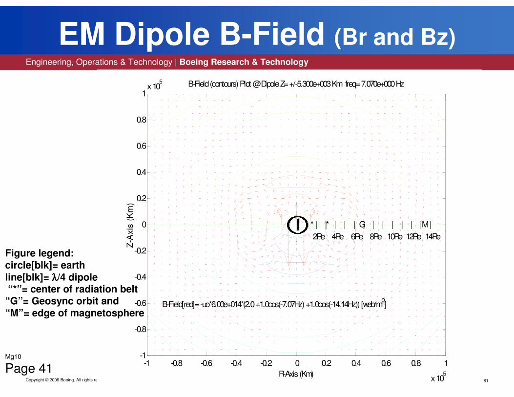
EOT_RT_template.ppt | 81
Engineering, Operations & Technology | Boeing Research & Technology
Copyright © 2009 Boeing. All rights reserved.
EM Dipole B-Field (Br and Bz)
Mg10
Page 41-1 -0.8 -0.6 -0.4 -0.2 0 0.2 0.4 0.6 0.8 1
x 105
-1
-0.8
-0.6
-0.4
-0.2
0
0.2
0.4
0.6
0.8
1x 10
5 B-Field (contours) Plot @ Dipole Z= +/-5.300e+003 Km freq= 7.070e+000 Hz
R-Axis (Km)
Z-A
xis
(K
m)
B-Field[red]= -uo*6.00e+014*(2.0 +1.0cos(-7.07Hz) +1.0cos(-14.14Hz)) [web/m2]
*********************
*| | | | | | | | | | | | |
2Re 4Re 6Re 8Re 10Re 12Re 14Re
------------------------------------------------------------------------------------------------------------------------------------------------------------------------------------------------------------------------------------------------------------------------------------------------------------------------------------------------------------------------- * * G M
Figure legend: circle[blk]= earth
line[blk]= λλλλ/4 dipole “*”= center of radiation belt
“G”= Geosync orbit and “M”= edge of magnetosphere

EOT_RT_template.ppt | 82
Engineering, Operations & Technology | Boeing Research & Technology
Copyright © 2009 Boeing. All rights reserved.
Figure 41) “EM Dipole B-field (Br and Bz)” shows the complete (AC) magnetic B-field[red] vectors (arrows) and constant contour plots in 3D space. As can be seen from the figure
there are maximum magnetic potentials at each dipole end one positive (N) and one
negative (S) both attenuating to zero at (z= λ) on the Z-axis. Similarly, there is a negative
B-field maximum at the inner radiation belt center (λ/4) and positive maximums at the outer radiation belt center (λ/2), at Geosync (λ) and the magnetosphere (2λ). The (AC) dynamic terms (real) cause the magnetic field to group or cluster at the harmonic intervals rather then evenly distributed like (DC). While the complex terms (imaginary) cause the field to
rotate or move in loops and sub-loops at distances less then λ. However, the overall magnetic field does attenuate inversely as the square of the distance (1/R^2). Note the figure only shows half the AC cycle. In the next half cycle the magnetic field vectors all
reverse direction.
Main points:
1) Complete magnetic B-field vectors out to 2λ2) N and S magnetic dipole potentials3) The (AC) causes the B-field pattern to cluster at harmonic intervals
4) Near field pattern (< λ) loops caused by complex terms 5) B-field attenuates as the square of the distance (1/R^2)
6) Only a half cycle of (AC) shown, fields reverse next half cycle

EOT_RT_template.ppt | 83
Engineering, Operations & Technology | Boeing Research & Technology
Copyright © 2009 Boeing. All rights reserved.
EM Dipole B-Field (Br and Bz)[Detailed View]
Mg10
Page 41A-5 -4 -3 -2 -1 0 1 2 3 4 5
x 104
-5
-4
-3
-2
-1
0
1
2
3
4
5x 10
4 B-Field (contours) Plot @ Dipole Z= +/-5.300e+003 Km freq= 7.070e+000 Hz
R-Axis (Km)
Z-A
xis
(K
m)
B-Field[red]= -uo*6.00e+014*(2.0 +1.0cos(-7.07Hz) +1.0cos(-14.14Hz)) [web/m2]
***********
*
*
*
*
*
*
*
*
*
*
*
| | | | | | | |
2Re 4Re 6Re 8Re 10Re
-------------------------------
------------------------------------------------------------------------------------------------------------------------------------------------------------------------------------------------------------------------------------------------------------------------------------------------------------
------------------------------ * * G
Figure legend: circle[blk]= earth
line[blk]= λλλλ/4 dipole “*”= center of radiation belt
“G”= Geosync orbit
EOT_RT_template.ppt | 84
Engineering, Operations & Technology | Boeing Research & Technology
Copyright © 2009 Boeing. All rights reserved.
Figure 41A) “EM Dipole B-Field (Detailed View)” is the same B-field data as in
figure 41 showing only a 50,000Km close-up. This detailed view displays the Magnetic B-field vectors and potential contours more clearly.
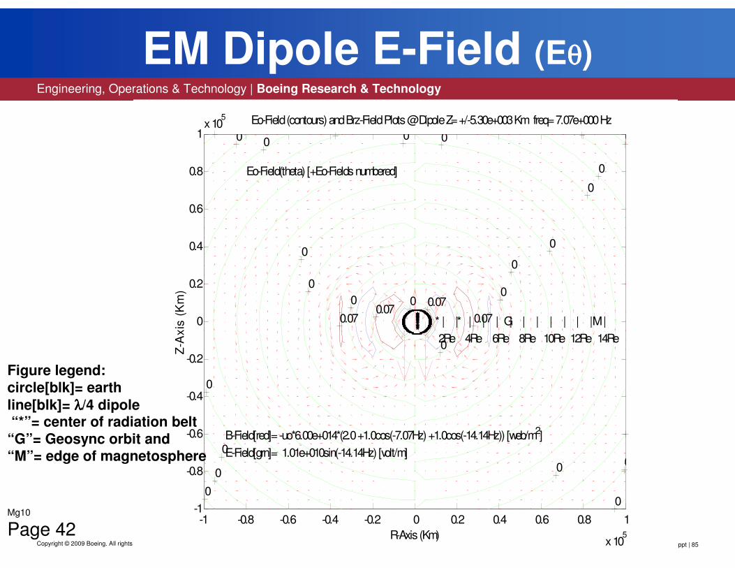
EOT_RT_template.ppt | 85
Engineering, Operations & Technology | Boeing Research & Technology
Copyright © 2009 Boeing. All rights reserved.
EM Dipole E-Field (Eθθθθ)
Mg10
Page 42-1 -0.8 -0.6 -0.4 -0.2 0 0.2 0.4 0.6 0.8 1
x 105
-1
-0.8
-0.6
-0.4
-0.2
0
0.2
0.4
0.6
0.8
1x 10
5
0
0
0
0
0
0
0
0
0
0
0
0
0
0
0
0
0
00
0
00
0
0
0.07
0.07 0.070.07
Eo-Field (contours) and Brz-Field Plots @ Dipole Z= +/-5.30e+003 Km freq= 7.07e+000 Hz
R-Axis (Km)
Z-A
xis
(K
m)
Eo-Field(theta) [+Eo-Fields numbered]
B-Field[red]= -uo*6.00e+014*(2.0 +1.0cos(-7.07Hz) +1.0cos(-14.14Hz)) [web/m2]
E-Field[grn]= 1.01e+010sin(-14.14Hz) [volt/m]
*********************
*| | | | | | | | | | | | |
2Re 4Re 6Re 8Re 10Re 12Re 14Re
------------------------------------------------------------------------------------------------------------------------------------------------------------------------------------------------------------------------------------------------------------------------------------------------------------------------------------------------------------------------- * * G M
Figure legend: circle[blk]= earth
line[blk]= λλλλ/4 dipole “*”= center of radiation belt
“G”= Geosync orbit and “M”= edge of magnetosphere

EOT_RT_template.ppt | 86
Engineering, Operations & Technology | Boeing Research & Technology
Copyright © 2009 Boeing. All rights reserved.
Figure 42) “EM Dipole E-field (Eθ)” shows the same (AC) magnetic B-field[red] vectors (arrows) with the electric E-field[grn] superimposed on it. As can be
seen from the figure the complete electric E-field is composed of shells of alternating spin polarity with nodes at the magnetic dipole ends. Only the
positive part (green outline) of the shell is shown for clarity. Positive is defined as rotating into the page. Similar to the (AC) magnetic B-field harmonic clustering
the (AC) electric E-field shell pattern rotates at the second harmonic (2θ). Also, the overall electric field does attenuate inversely as the square of the distance
(1/R^2). Note the figure only shows half the AC cycle. In the next half cycle the magnetic field vectors all reverse direction and the electric field shells oscillate
the other direction.
Main points:
1) Complete electric E-field and magnetic B-field vectors out to 2λ2) The (AC) causes the E-field to form alternate polarity spherical shells3) that oscillate at the second harmonic frequency4) E-field also attenuates as the square of the distance (1/R^2)
5) Only a half cycle of (AC) shown, both fields reverse next half cycle

EOT_RT_template.ppt | 87
Engineering, Operations & Technology | Boeing Research & Technology
Copyright © 2009 Boeing. All rights reserved.
EM Dipole E-Field (Eθθθθ)[Detailed View]
-5 -4 -3 -2 -1 0 1 2 3 4 5
x 104
-5
-4
-3
-2
-1
0
1
2
3
4
5x 10
4
0
0
0
0
0
0
0
0
0
0
0
00
0.07
0.07
0.07
0.07
Eo-Field (contours) and Brz-Field Plots @ Dipole Z= +/-5.30e+003 Km freq= 7.07e+000 Hz
R-Axis (Km)
Z-A
xis
(K
m)
Eo-Field(theta) [+Eo-Fields numbered]
B-Field[red]= -uo*6.00e+014*(2.0 +1.0cos(-7.07Hz) +1.0cos(-14.14Hz)) [web/m2]
E-Field[grn]= 1.01e+010sin(-14.14Hz) [volt/m]
***********
*
*
*
*
*
*
*
*
*
*
*
| | | | | | | |
2Re 4Re 6Re 8Re 10Re
-------------------------------
------------------------------------------------------------------------------------------------------------------------------------------------------------------------------------------------------------------------------------------------------------------------------------------------------------
------------------------------ * * G
Mg10
Page 42A
Figure legend: circle[blk]= earth
line[blk]= λλλλ/4 dipole “*”= center of radiation belt
“G”= Geosync orbit
EOT_RT_template.ppt | 88
Engineering, Operations & Technology | Boeing Research & Technology
Copyright © 2009 Boeing. All rights reserved.
Figure 42A) “EM Dipole E-Field (Detailed View)” is the same E-field data as in figure 42 showing only a 50,000Km close-up. This detailed view displays the Magnetic B-
field vectors and Electric contours more clearly.

EOT_RT_template.ppt | 89
Engineering, Operations & Technology | Boeing Research & Technology
Copyright © 2009 Boeing. All rights reserved.
EM Dipole All Fields
-1 -0.8 -0.6 -0.4 -0.2 0 0.2 0.4 0.6 0.8 1
x 105
-1
-0.8
-0.6
-0.4
-0.2
0
0.2
0.4
0.6
0.8
1x 10
5
0
0
0
0
0
0
0
0
0
0
0
0
0
0
0
0
0
00
00
00
0
0.070.07
0.070.07
F-Fields Plot @ Dipole Z= +/-5.300e+003 Km freq= 7.070e+000 Hz
R-Axis (Km)
Z-A
xis
(K
m)
Eo-Field(theta) [+Eo-Fields numbered]
B-Field[red]= -uo*6.00e+014*(2.0 +1.0cos(-7.07Hz) +1.0cos(-14.14Hz)) [web/m2]
E-Field[grn]= 1.01e+010sin(-14.14Hz) [volt/m]
F-Field[blu]= 1.01e+019*(1.0cos(-7.07Hz) +1.5cos(-14.14Hz) +1.0cos(-21.21Hz) +1.1cos(-28.28Hz)) [nt/m2]
*********************
*| | | | | | | | | | | | |
2Re 4Re 6Re 8Re 10Re 12Re 14Re
------------------------------------------------------------------------------------------------------------------------------------------------------------------------------------------------------------------------------------------------------------------------------------------------------------------------------------------------------------------------- * * G M
Mg10
Page 43
Figure legend: circle[blk]= earth
line[blk]= λλλλ/4 dipole “*”= center of radiation belt
“G”= Geosync orbit and “M”= edge of magnetosphere
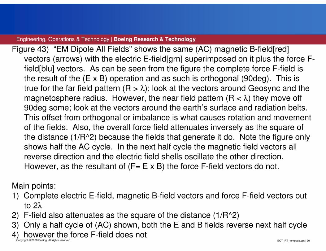
EOT_RT_template.ppt | 90
Engineering, Operations & Technology | Boeing Research & Technology
Copyright © 2009 Boeing. All rights reserved.
Figure 43) “EM Dipole All Fields” shows the same (AC) magnetic B-field[red]
vectors (arrows) with the electric E-field[grn] superimposed on it plus the force F-
field[blu] vectors. As can be seen from the figure the complete force F-field is the result of the (E x B) operation and as such is orthogonal (90deg). This is
true for the far field pattern (R > λ); look at the vectors around Geosync and the
magnetosphere radius. However, the near field pattern (R < λ) they move off 90deg some; look at the vectors around the earth’s surface and radiation belts.
This offset from orthogonal or imbalance is what causes rotation and movement
of the fields. Also, the overall force field attenuates inversely as the square of the distance (1/R^2) because the fields that generate it do. Note the figure only
shows half the AC cycle. In the next half cycle the magnetic field vectors all
reverse direction and the electric field shells oscillate the other direction. However, as the resultant of (F= E x B) the force F-field vectors do not.
Main points:
1) Complete electric E-field, magnetic B-field vectors and force F-field vectors out
to 2λ2) F-field also attenuates as the square of the distance (1/R^2)
3) Only a half cycle of (AC) shown, both the E and B fields reverse next half cycle
4) however the force F-field does not
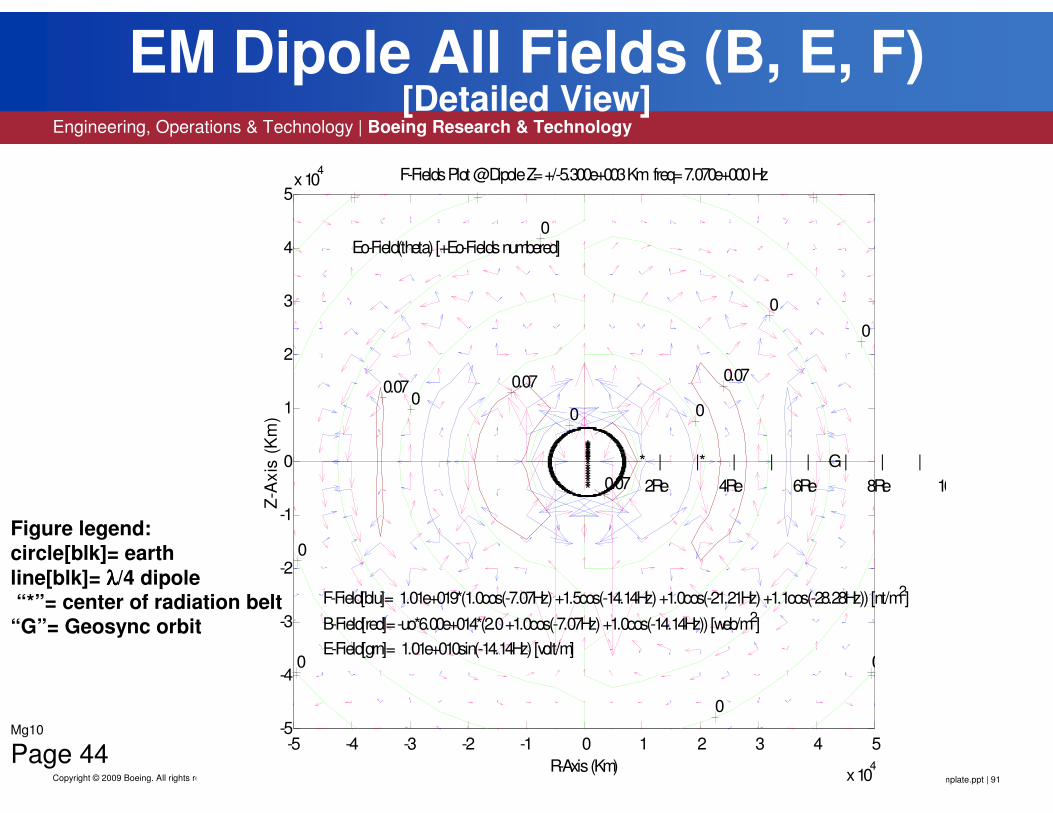
EOT_RT_template.ppt | 91
Engineering, Operations & Technology | Boeing Research & Technology
Copyright © 2009 Boeing. All rights reserved.
EM Dipole All Fields (B, E, F) [Detailed View]
-5 -4 -3 -2 -1 0 1 2 3 4 5
x 104
-5
-4
-3
-2
-1
0
1
2
3
4
5x 10
4
0
0
0
0
0
0
0
0
0
0
0
00
0.07
0.070.070.07
F-Fields Plot @ Dipole Z= +/-5.300e+003 Km freq= 7.070e+000 Hz
R-Axis (Km)
Z-A
xis
(K
m)
Eo-Field(theta) [+Eo-Fields numbered]
B-Field[red]= -uo*6.00e+014*(2.0 +1.0cos(-7.07Hz) +1.0cos(-14.14Hz)) [web/m2]
E-Field[grn]= 1.01e+010sin(-14.14Hz) [volt/m]
F-Field[blu]= 1.01e+019*(1.0cos(-7.07Hz) +1.5cos(-14.14Hz) +1.0cos(-21.21Hz) +1.1cos(-28.28Hz)) [nt/m2]
***********
*
*
*
*
*
*
*
*
*
*
*
| | | | | | | |
2Re 4Re 6Re 8Re 10Re
-------------------------------
------------------------------------------------------------------------------------------------------------------------------------------------------------------------------------------------------------------------------------------------------------------------------------------------------------------------------------------ * * G
Mg10
Page 44
Figure legend: circle[blk]= earth
line[blk]= λλλλ/4 dipole “*”= center of radiation belt
“G”= Geosync orbit
EOT_RT_template.ppt | 92
Engineering, Operations & Technology | Boeing Research & Technology
Copyright © 2009 Boeing. All rights reserved.
Figure 44) “EM Dipole All Fields (Detailed View)” is the same all fields data as in figure 43 only showing a 50,000Km close-up. This detailed view displays the
Magnetic B-field[red] vectors, Force F-field[blu] vectors and Electric contours[grn] more clearly.

EOT_RT_template.ppt | 93
Engineering, Operations & Technology | Boeing Research & Technology
Copyright © 2009 Boeing. All rights reserved.
Gravity Conclusions
• At wavelengths less then one lambda the fields are not at a perfect 90deg angle.
• Because the imaginary part of the EM field equations is greater (has more effect) then that of the real part.
• This imbalance causes the fields to precess (rotate) in these areas:
• Planet• Inner radiation belt• Outer radiation belt
• At wavelengths equal to or greater then one lambda the fields stabilize (90deg angle):
• Geo Sync Orbit• Edge of Magnetosphere
• Magnetic dipole length λλλλ/4 (10,606Km)Mg10
Page 45

EOT_RT_template.ppt | 94
Engineering, Operations & Technology | Boeing Research & Technology
Copyright © 2009 Boeing. All rights reserved.
Figure 45) “Gravity Conclusions” These are the findings and results of the “Study
of Gravity (part 2)” the accelerating force field is indeed connected to the (EM)
ElectroMagnetic fields. However, at distances less then lambda (λ) the field vectors are not orthogonal (90deg) because the near field pattern (imaginary
part) has more control. This results in an imbalance causing the near field patterns to precess and rotate (spin). The near field forces mainly affect the
planet and the two radiation belts. Further out at distances of lambda (λ) or more the far field pattern stabilizes things; the field vectors become orthogonal
(90deg). The far field forces mainly affect Geosync orbit and the
magnetosphere shell. The earth’s magnetic dipole length is λ/4 at the
fundamental frequency or λ/2 at the second harmonic. The preceding figures show the complete electric, magnetic and force field interactions.
Main points:
1) The accelerating force is connected to the EM fields
2) The near field pattern (< λ) effects the planet and radiation belts
3) The far field pattern (>= λ) effects Geosync orbit and the magnetosphere
4) The earth’s magnetic dipole length is λ/4 at the fundamental frequency
EOT_RT_template.ppt | 95
Engineering, Operations & Technology | Boeing Research & Technology
Copyright © 2009 Boeing. All rights reserved.
Gravity Conclusions (cont)
• Gravity is an accelerating force field which appears to be generated by a circular (Eθθθθ) electric field and polar dipole (Br, Bz) magnetic fields. These electric and magnetic fields are composed of (AC) waves. The electric field is only the second harmonic. While the magnetic field has a (DC) term along with two harmonics. The E and B fields are then mixed (ExB) to produce the four harmonic beat frequencies that produce the accelerating gravitational force field.
• This field in turn drives a leaky resonate cavity system known as “Schumann Resonance”. This standing wave pattern determines the structure of the planet, effects the weather and human life itself. NASA has Schumann oscillators on board the space shuttles for this reason. Mg10
Page 46

EOT_RT_template.ppt | 96
Engineering, Operations & Technology | Boeing Research & Technology
Copyright © 2009 Boeing. All rights reserved.
Figure 46) “Gravity Conclusions (cont)” the accelerating force commonly called “gravity’ seems to be the resultant force generated from the interaction (F= E x B) of the earth’s electric and magnetic
fields. The electric E-field oscillates (AC) in the circular direction (θ-axis) at the second harmonic frequency. Kind of like the agitator in a washing machine (back and forth). E-field is shell shape with maximums at the equator and nodes at both the poles; these shells alternate in polarity and therefore spin direction. The magnetic B-field oscillates in the polar direction (R and Z axis) with a constant term (DC), a fundamental term and second harmonic with relative amplitudes of: B0= 2*B1. These two (E and B) orthogonal fields are then mixed producing a third or resultant orthogonal field. This accelerating force “gravity” field consists of four heterodyne (beat) frequencies with relative amplitudes of: F2= 1.5*F1, F3= F1 and F4= 1.2*F1. The force F-field in turn drives the earths leaky resonate cavity system (70% efficient) producing four harmonic standing waves known as “Schumann Resonance”. These waves determine magnetic anomalies, pole movements, weather patterns and effect human life itself.
Main points:1) Gravity is the result of the earth’s electric and magnetic fields2) The electric E-field is composed of one second harmonic term3) The magnetic B-field is composed of three terms: a constant, fundamental and second harmonic4) The accelerating force field is composed of four harmonic terms: fundamental, second, third and
fourth harmonics5) The earth’s resonate cavity generates the waves known as “Schumann Resonance”6) NASA has Schumann oscillators onboard the space shuttle
EOT_RT_template.ppt | 97
Engineering, Operations & Technology | Boeing Research & Technology
Copyright © 2009 Boeing. All rights reserved.
SPACE DRIVES
APPLICATIONSThe design of the following space drives are based on data from the preceding study of gravity along with other current technologies.
Mg10
Page 47
EOT_RT_template.ppt | 98
Engineering, Operations & Technology | Boeing Research & Technology
Copyright © 2009 Boeing. All rights reserved.
Figure 47) “Space Drives” The following figures propose two possible applications
for the information gained from this “Study of Gravity” along with other current technologies. The first space drive system is the Tesla Drive which is based on his electric motor design along with the gravity harmonics. Its operation would be
limited to near earth applications. The second space drive system is the Warp
Drive which is based on a synchrotron design. Its operation is intended for deep
space applications.

EOT_RT_template.ppt | 99Copyright © 2009 Boeing. All rights reserved.
TESLA DRIVE
Mg10
Page 48
EOT_RT_template.ppt | 100
Engineering, Operations & Technology | Boeing Research & Technology
Copyright © 2009 Boeing. All rights reserved.
Figure 48) “Tesla Drive” is a proposed space drive based on the information gained from this “Study of Gravity”. Its operating principle is based on that of the
electric AC induction motor invented by Tesla (hence the name). The electric motor design has been around for about a century so it is nothing new, only this application is! The primary difference being the motor is now turned on end with the force vectors in the vertical direction rather than circular (rotary). The next few
figures are a short tutorial on electric motor basics starting with a standard rotary
motor followed by a linear one. This is background material for understanding how the basic motor principle can be modified.
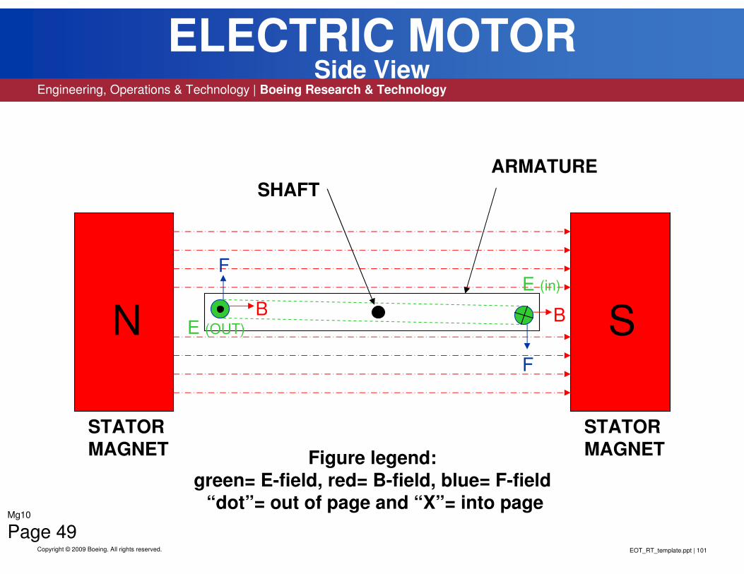
EOT_RT_template.ppt | 101
Engineering, Operations & Technology | Boeing Research & Technology
Copyright © 2009 Boeing. All rights reserved.
ELECTRIC MOTORSide View
N SB
F
E (OUT)B
F
E (in)
STATOR
MAGNET
STATOR
MAGNET
ARMATURE
Mg10
Page 49
SHAFT
Figure legend:
green= E-field, red= B-field, blue= F-field “dot”= out of page and “X”= into page

EOT_RT_template.ppt | 102
Engineering, Operations & Technology | Boeing Research & Technology
Copyright © 2009 Boeing. All rights reserved.
ELECTRIC MOTORTop View
N S
E E
F (out) F (in)
B B
ARMATURE
STATOR
MAGNET
STATOR
MAGNET
Mg10
Page 50
SHAFT
Figure legend: green= E-field, red= B-field, blue= F-field
“dot”= out of page and “X”= into page
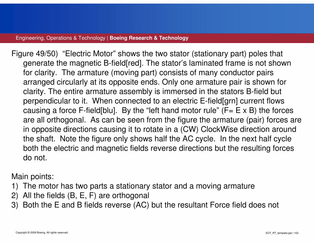
EOT_RT_template.ppt | 103
Engineering, Operations & Technology | Boeing Research & Technology
Copyright © 2009 Boeing. All rights reserved.
Figure 49/50) “Electric Motor” shows the two stator (stationary part) poles that
generate the magnetic B-field[red]. The stator’s laminated frame is not shown
for clarity. The armature (moving part) consists of many conductor pairs arranged circularly at its opposite ends. Only one armature pair is shown for
clarity. The entire armature assembly is immersed in the stators B-field but perpendicular to it. When connected to an electric E-field[grn] current flows
causing a force F-field[blu]. By the “left hand motor rule” (F= E x B) the forces
are all orthogonal. As can be seen from the figure the armature (pair) forces are in opposite directions causing it to rotate in a (CW) ClockWise direction around
the shaft. Note the figure only shows half the AC cycle. In the next half cycle
both the electric and magnetic fields reverse directions but the resulting forces do not.
Main points:
1) The motor has two parts a stationary stator and a moving armature
2) All the fields (B, E, F) are orthogonal 3) Both the E and B fields reverse (AC) but the resultant Force field does not

EOT_RT_template.ppt | 104
Engineering, Operations & Technology | Boeing Research & Technology
Copyright © 2009 Boeing. All rights reserved.
LINEAR INDUCTION MOTORSide View
N
S
N
S
E
F F FF
E
E
E
Front side stator magnets removed for clarity
ARMATURE
Mg10
Page 51
Figure legend: green= E-field, red= B-field, blue= F-field
“dot”= out of page and “X”= into page
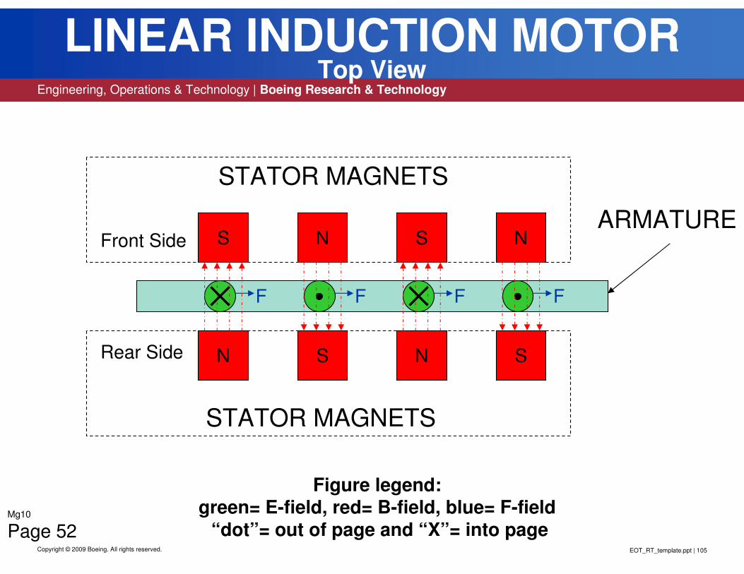
EOT_RT_template.ppt | 105
Engineering, Operations & Technology | Boeing Research & Technology
Copyright © 2009 Boeing. All rights reserved.
LINEAR INDUCTION MOTORTop View
N S N S
S N S N
F F F F
Rear Side
Front Side
STATOR MAGNETS
STATOR MAGNETS
ARMATURE
Mg10
Page 52
Figure legend: green= E-field, red= B-field, blue= F-field
“dot”= out of page and “X”= into page

EOT_RT_template.ppt | 106
Engineering, Operations & Technology | Boeing Research & Technology
Copyright © 2009 Boeing. All rights reserved.
Figure 51/52) “Linear Induction Motor” is a motor design that has had its circular armature and stator unwrapped and laid flat (linear). The armature is now a flat
conductive plate which is still located between the stator pole magnets and is immersed in its B-field. The linear motor functions on the same “left hand motor
rule” so all the resultant orthogonal forces now push the armature to the right. The front side magnets are not shown for clarity so the electric (eddy) current
path in the armature can be seen. Note the figure only shows half the AC
cycle. In the next half cycle both the electric and magnetic fields reverse
directions but the resulting forces do not.
Main points:1) The motor has two parts a stationary stator and a moving armature
2) All the fields (B, E, F) are orthogonal
3) Both the E and B fields reverse (AC) but the resultant Force field does not
4) In principle a linear motor functions identical to a rotary one
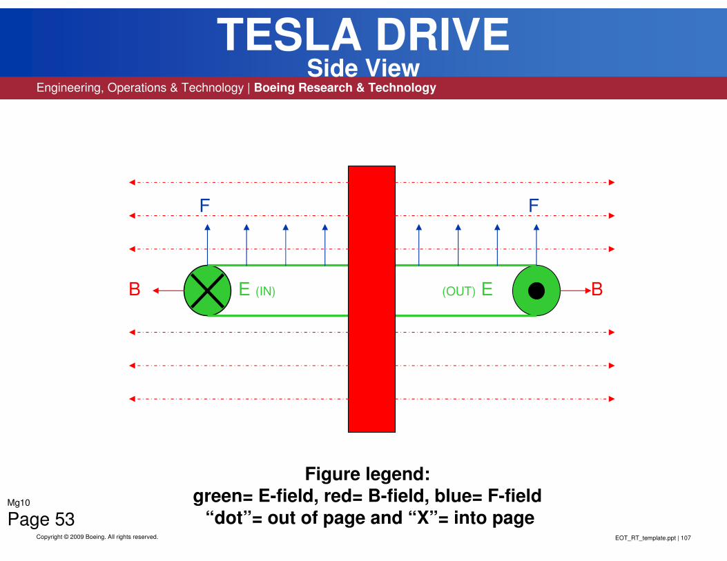
EOT_RT_template.ppt | 107
Engineering, Operations & Technology | Boeing Research & Technology
Copyright © 2009 Boeing. All rights reserved.
TESLA DRIVESide View
F
B
F
E (IN) B(OUT) E
Mg10
Page 53
Figure legend: green= E-field, red= B-field, blue= F-field
“dot”= out of page and “X”= into page
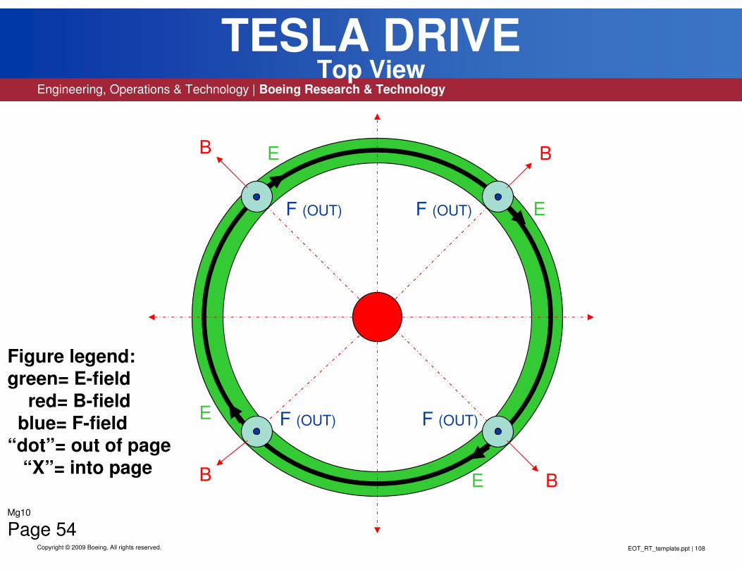
EOT_RT_template.ppt | 108
Engineering, Operations & Technology | Boeing Research & Technology
Copyright © 2009 Boeing. All rights reserved.
TESLA DRIVETop View
B
B
B
B
F (OUT)
F (OUT) F (OUT)
F (OUT)
E
E
E
E
Mg10
Page 54
Figure legend: green= E-field
red= B-field blue= F-field
“dot”= out of page “X”= into page
EOT_RT_template.ppt | 109
Engineering, Operations & Technology | Boeing Research & Technology
Copyright © 2009 Boeing. All rights reserved.
Figure 53/54) “Tesla Drive” is a motor design that has had its armature winding (conductive ring) rotated 90deg so all the resultant forces now point in the same direction (up) similar to the linear motor but still in a circular shape. Likewise the armature is immersed in the magnetic field which is now radial. One advantage of this configuration is that it allows the motor to be run in a tuned or resonate mode. If the magnetic pole is half wavelength long and the ring is one wavelength in circumference the system will resonate at its fundamental frequency. The operating frequency varies inversely as the size of the motor. If the center of mass and the center of force coincide then nothing happens, but if don’t then there is a force generated. The easy part is getting the resonate device running, the difficult part is synchronizing it to the earth’s harmonics so it has something to push against. Note the figure only shows half the AC cycle. In the next half cycle both the electric and magnetic fields reverse directions but the resulting forces do not.
Main points:1) Circular shaped armature coil (lift ring)2) All the fields (B, E, F) are orthogonal – “left hand motor rule”3) Both the E and B fields reverse (AC) but the resultant Force field does not4) Configuration allows for resonance mode operations5) In principle it would function identical to a rotary motor6) Must be synchronized to the earth’s field
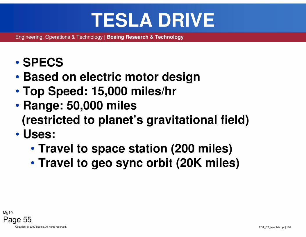
EOT_RT_template.ppt | 110
Engineering, Operations & Technology | Boeing Research & Technology
Copyright © 2009 Boeing. All rights reserved.
TESLA DRIVE
• SPECS• Based on electric motor design • Top Speed: 15,000 miles/hr• Range: 50,000 miles (restricted to planet’s gravitational field)
• Uses:• Travel to space station (200 miles)• Travel to geo sync orbit (20K miles)
Mg10
Page 55

EOT_RT_template.ppt | 111
Engineering, Operations & Technology | Boeing Research & Technology
Copyright © 2009 Boeing. All rights reserved.
Figure 55) “Tesla Drive” lists some of the general specifications for this propulsion system. The major one being that it is based on tried and true 100 year old
motor technology nothing new. Therefore, it has a high probability of running
with good reliability. This reliability is further increased by the fact that it has only one moving part. Reliability is one of the primary requirements for space operated systems, as service calls are to say the least difficult! Rough numbers
show a top speed around 15K miles/hr which is capable of achieving (LEO) Low
Earth Orbit. The problem is that its operation is restricted to the earths
gravitational field so its maximum range is therefore less than 50K miles. However, it still would be a travel improvement to and from the space station or
further out to GeoSync orbit.
Main points:
1) Based on 100 year old motor technology
2) Simple reliable design good for space operations3) Range limited to the earth’s gravitational field

EOT_RT_template.ppt | 112Copyright © 2009 Boeing. All rights reserved.
WARP DRIVE PARAMOUNT PICTURES: STAR TREK
Mg10
Page 56

EOT_RT_template.ppt | 113
Engineering, Operations & Technology | Boeing Research & Technology
Copyright © 2009 Boeing. All rights reserved.
Figure 56) “Warp Drive” is another proposed space drive that could be used for
deep space propulsion as it is not restricted to a planet’s gravitational field. Being an old Star Trek fan have to give credit for the name where it’s due. The operating
principle is based on that of the synchrotron or as it is more commonly called an atom smasher. This design has been around for about a half century so it is also nothing new, but this application is! The problem with space travel is the great
distances involved, to get anywhere in reasonable time you must go (very) fast.
According to physics the maximum speed possible is the speed of light (C=
186,284 miles/sec). In looking around the only machines that operate anywhere close to this speed are atom smashers so this becomes the starting point of the
design.
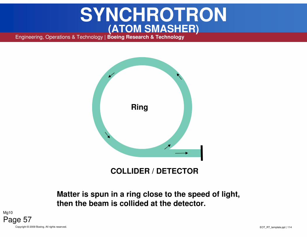
EOT_RT_template.ppt | 114
Engineering, Operations & Technology | Boeing Research & Technology
Copyright © 2009 Boeing. All rights reserved.
SYNCHROTRON(ATOM SMASHER)
COLLIDER / DETECTOR
Matter is spun in a ring close to the speed of light,
then the beam is collided at the detector.
Ring
Mg10
Page 57
EOT_RT_template.ppt | 115
Engineering, Operations & Technology | Boeing Research & Technology
Copyright © 2009 Boeing. All rights reserved.
Figure 57) “Synchrotron (atom smasher)” shows the general outline of the machine to be ring shaped. The operating principle is as follows: matter mainly
hydrogen is accelerated in a ring (around and around) until its speed
approaches that of light (.8-.9C). The beam of matter is then diverted out of the ring to collide with a target which contains a detector to record what happened. It is a laboratory device used in the study of sub-atomic particles and nuclear
physics.
Main points:
1) Ring shaped device
2) Accelerates matter close to the speed of light
3) Beam is diverted to target/detector
4) Used in the study of sub-atomic particles
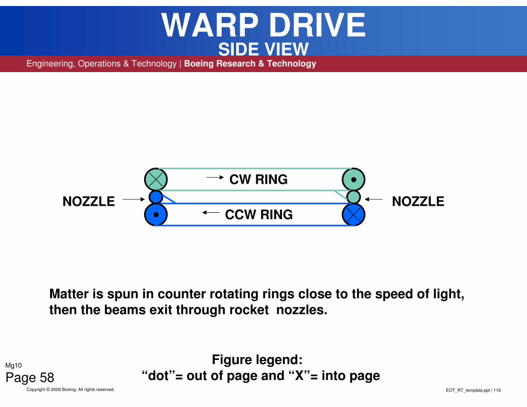
EOT_RT_template.ppt | 116
Engineering, Operations & Technology | Boeing Research & Technology
Copyright © 2009 Boeing. All rights reserved.
WARP DRIVESIDE VIEW
CCW RING
CW RING
NOZZLENOZZLE
Matter is spun in counter rotating rings close to the speed of light,
then the beams exit through rocket nozzles.
Mg10
Page 58
Figure legend:
“dot”= out of page and “X”= into page

EOT_RT_template.ppt | 117
Engineering, Operations & Technology | Boeing Research & Technology
Copyright © 2009 Boeing. All rights reserved.
WARP DRIVETOP VIEW
COUNTER
ROTATINGRINGS
NOZZLENOZZLE
Matter is spun in counter rotating rings close to the speed of light,
then the beams exit through rocket nozzles.Mg10
Page 59

EOT_RT_template.ppt | 118
Engineering, Operations & Technology | Boeing Research & Technology
Copyright © 2009 Boeing. All rights reserved.
Figure 58/59) “Warp Drive” Shows the major working parts of this propulsion system. It is similar to the synchrotron’s operation in that matter is spun up in
rings. Each ring spins in opposite directions to counter act (null out) circular torque, they must be operated in pairs. The difference is that instead of
crashing into a target the beams now exit through rocket type nozzles
producing thrust. The two nozzles are on opposite sides of the device and
both pointing in the same direction to produce a combined forward movement.
The difficult part of this design is impedance matching the nozzles to space conditions to achieve maximum thrust.
Main points:1) Similar to a synchrotron’s operation of ring acceleration
2) Counter rotating matter rings to null torque
3) Dual thrust rocket nozzles
4) Nozzles tuned for maximum thrust

EOT_RT_template.ppt | 119
Engineering, Operations & Technology | Boeing Research & Technology
Copyright © 2009 Boeing. All rights reserved.
WARP DRIVE
• SPECS• Based on Synchrotron design • Top Speed: 0.5c (300,000,000 miles/Hr)• Range: (limited to size of fuel tank)• Uses:
• Space exploration• Interplanetary travel
Mg10
Page 60

EOT_RT_template.ppt | 120
Engineering, Operations & Technology | Boeing Research & Technology
Copyright © 2009 Boeing. All rights reserved.
Figure 60) “Warp Drive” lists some of the general specifications of this propulsion system. The major one being that it is based on tried and true 50 year old synchrotron technology nothing new. Therefore, it also has a high probability of running with good reliability. If the nozzles can be correctly matched (tuned) it should be possible to convert approximately half the ring velocity into forward thrust
giving it a top speed around .4-.5C. The problem is that it is an open loop system
so matter is lost in the propulsion process, this limits its range to the size of the gas
tank in this case water! However, (miles/sec) miles per second are a big improvement in speed over (miles/hr) miles per hour when it comes to the distances
of space travel.
Main points:
1) Based on 50 year old synchrotron technology
2) Also a simple reliable design good for space operations
3) Nozzles must be tuned and operated in pairs4) Open loop process5) Range limited to the size of the gas tank
6) Safe fuel – water

EOT_RT_template.ppt | 1/6/2009 | 121
BOEING is a trademark of Boeing Management Company.
Copyright © 2009 Boeing. All rights reserved.
Thank you
Mg10
Page 61