study of gas flow dynamics in porous and granular media with
TRANSCRIPT

Study of Gas Flow Dynamics in Porous and
Granular Media with Laser-Polarized 129Xe NMRby
Ruopeng WangSubmitted to the Department of Nuclear Science and Engineering
in partial fulfillment of the requirements for the degree ofDoctor of Philosophy
at theMASSACHUSETTS INSTITUTE OF TECHNOLOGY
February 2005c© Massachusetts Institute of Technology 2005. All rights reserved.
Author . . . . . . . . . . . . . . . . . . . . . . . . . . . . . . . . . . . . . . . . . . . . . . . . . . . . . . . . . . . . . .Department of Nuclear Science and Engineering
Feb 1, 2005
Certified by. . . . . . . . . . . . . . . . . . . . . . . . . . . . . . . . . . . . . . . . . . . . . . . . . . . . . . . . . .Ronald L. Walsworth
Senior Lecturer, Harvard-Smithsonian Center for AstrophysicsThesis Supervisor
Certified by. . . . . . . . . . . . . . . . . . . . . . . . . . . . . . . . . . . . . . . . . . . . . . . . . . . . . . . . . .David G. Cory
Professor, Department of Nuclear Science and Engineering, M.I.T.Thesis Supervisor
Read by . . . . . . . . . . . . . . . . . . . . . . . . . . . . . . . . . . . . . . . . . . . . . . . . . . . . . . . . . . . . .Donald Candela
Professor, Department of Physics, University of MassachusettsThesis Reader
Read by . . . . . . . . . . . . . . . . . . . . . . . . . . . . . . . . . . . . . . . . . . . . . . . . . . . . . . . . . . . . .Alan P. Jasanoff
Associate Professor, Department of Nuclear Science and Engineering,M.I.T.
Thesis ReaderAccepted by . . . . . . . . . . . . . . . . . . . . . . . . . . . . . . . . . . . . . . . . . . . . . . . . . . . . . . . . .
Jeffrey A. CoderreAssociate Professor, Department of Nuclear Science and Engineering,
Chairman, Department Committee on Graduate Students

2

Study of Gas Flow Dynamics in Porous and Granular Media
with Laser-Polarized 129Xe NMR
by
Ruopeng Wang
Submitted to the Department of Nuclear Science and Engineeringon Feb 1, 2005, in partial fulfillment of the
requirements for the degree ofDoctor of Philosophy
Abstract
This thesis presents Nuclear Magnetic Resonance (NMR) studies of gas flow dynamicsin porous and granular media by using laser-polarized 129Xe. Two different physicalprocesses, the gas transport in porous rock cores and the mass exchanges betweendifferent phases in fluidized granular systems, were investigated and new experimen-tal methods were designed to measure several important parameters characterizingthe two systems. Methods for measuring the parameters had been either unavailableor significantly limited previously. The research involved modeling the gas flow inporous and granular media by relating the dynamics of spin magnetization to the in-teresting parameters, as well as correspondingly designing new measurement methodsand verifying them on the laboratory test beds.
We proposed a simple method to measure two important parameters of reservoirrocks, permeability and effective porosity, by probing the flow front of laser-polarizedxenon gas inside the rock cores. The method was thoroughly tested on different cat-egories of rocks with permeability values spanning two orders of magnitude, and theresults were in agreement with those from the established techniques. The unique-ness in the work is that the fast method developed is capable of measuring the twoparameters simultaneously on the same setup.
Bubble-emulsion exchange and emulsion-adsorption exchange in a fluidized bedare two processes crucial to the efficiency of many chemical reactors working in bub-bling regime. We used differences in T2 and chemical shift to contrast the threephases in the xenon spectra, and designed methods to measure the inter-phase ex-change rates. The measured results of the bubble-emulsion and emulsion-adsorptionexchange rates agreed well with predictions based on available theory. Our approachis the first to non-invasively probe natural bubbles in a three-dimensional bed, andto measure the exchange rate between the emulsion phase and multiple bubbles.
Thesis Supervisor: Ronald L. WalsworthTitle: Senior Lecturer, Harvard-Smithsonian Center for Astrophysics
3

Thesis Supervisor: David G. CoryTitle: Professor, Department of Nuclear Science and Engineering, M.I.T.
4

Acknowledgments
This thesis would not have come into being without the help from the many colleagues
and friends during my recent acdemeic years. I want to take this chance to express
my deep gratitude to those who helped me.
First I want to thank my thesis supervisor, Ronald Walsworth, for his support,
guide and encoragement. He provided me an excellent research environment, left me
enough freedom to do things the way I thought they should be done, and was always
available to discuss ideas and problems. I am very grateful for the opportunity to have
learned from and worked with him. Thank also goes to my advisor, David Cory, who
has been an excellent mentor providing me insightful directions and the discussions
with him have always been very helpful. I thank Ross Mair for his patience and
commitment in teaching me every aspect of NMR technology and guiding me through
the scientific practices. I owe a debt of gratitude to Matthew Rosen, who has spent lots
of time in helping design and build parts essential for the fluidized bed experiments,
and also in proofreading this thesis. I am fortunate to have an outstanding colaborator
and montor, Donald Candela at UMass. I offer my appreciation to him for the useful
discussion and guide in the field of fluidized granular media.
I also want to thank Tina Pavlin for the discussions on my research and the
helpful comments on my thesis draft. John Ng has been a friend and colleage great to
work with, and generously helped in running the experiments, as well as proofreading
my thesis. Leo Tsai and Mason Klein have lent me great ideas and experimental
apparatus from their work on vibro-fluidized bed. I am also indebted to David Phillips
and Glenn Wong for their help and inspiring guidance.
Finally I want to acknowledge the support and love from my family. The encor-
agement and understanding across the ocean from my parents has been crucial for
my completion of Ph.D. My wife Qing deserve my deepest thanks, for all that she
has done for me during these years. The accomplishment belongs to both of us.
5

6

Contents
1 Introduction 23
2 Nuclear Magnetic Resonance 27
2.1 Introduction . . . . . . . . . . . . . . . . . . . . . . . . . . . . . . . . 27
2.2 History . . . . . . . . . . . . . . . . . . . . . . . . . . . . . . . . . . . 27
2.3 Spin Dynamics . . . . . . . . . . . . . . . . . . . . . . . . . . . . . . 28
2.4 Relaxation . . . . . . . . . . . . . . . . . . . . . . . . . . . . . . . . . 31
2.4.1 Longitudinal Relaxation T1 . . . . . . . . . . . . . . . . . . . 32
2.4.2 Transverse Relaxation T2 . . . . . . . . . . . . . . . . . . . . . 33
2.4.3 Relaxation Mechanisms and Quantum-Mechanical Results . . 34
2.5 Chemical Shift . . . . . . . . . . . . . . . . . . . . . . . . . . . . . . 36
2.6 Susceptibility-Induced Shift and Line Broadening . . . . . . . . . . . 37
2.7 Diffusion and Measurement with NMR . . . . . . . . . . . . . . . . . 39
2.8 Diffusion . . . . . . . . . . . . . . . . . . . . . . . . . . . . . . . . . . 39
2.8.1 NMR Technique for Measuring Diffusion and Flow . . . . . . 40
2.9 Imaging . . . . . . . . . . . . . . . . . . . . . . . . . . . . . . . . . . 42
2.9.1 Principle . . . . . . . . . . . . . . . . . . . . . . . . . . . . . . 42
2.9.2 One-Dimensional Imaging . . . . . . . . . . . . . . . . . . . . 43
2.9.3 Two-Dimensional Imaging . . . . . . . . . . . . . . . . . . . . 45
3 NMR with Laser-Polarized 129Xe Gas 47
3.1 Introduction . . . . . . . . . . . . . . . . . . . . . . . . . . . . . . . . 47
3.2 Laser-Polarization of 129Xe . . . . . . . . . . . . . . . . . . . . . . . . 49
7

3.2.1 Spin-Exchange Optical Pumping . . . . . . . . . . . . . . . . 49
3.2.2 129Xe Polarization and Delivery System . . . . . . . . . . . . . 53
3.3 Spin relaxation of Gas-Phase 129Xe Polarization . . . . . . . . . . . . 56
3.3.1 T1 Relaxation . . . . . . . . . . . . . . . . . . . . . . . . . . . 56
3.3.2 T2 Relaxation . . . . . . . . . . . . . . . . . . . . . . . . . . . 57
3.4 Magnetic Resonance with Laser-Polarized 129Xe . . . . . . . . . . . . 58
3.4.1 Batch Mode . . . . . . . . . . . . . . . . . . . . . . . . . . . . 59
3.4.2 Continuous Flow . . . . . . . . . . . . . . . . . . . . . . . . . 64
4 Simultaneous Measurement of Rock Permeability and Effective Poros-
ity using Laser-Polarized Noble Gas NMR1 65
4.1 Introduction . . . . . . . . . . . . . . . . . . . . . . . . . . . . . . . . 65
4.2 Experimental Procedure . . . . . . . . . . . . . . . . . . . . . . . . . 68
4.3 Effective Porosity Measurement and Results . . . . . . . . . . . . . . 71
4.4 Permeability Measurement and Results . . . . . . . . . . . . . . . . . 74
4.5 Error Analysis . . . . . . . . . . . . . . . . . . . . . . . . . . . . . . . 79
4.6 Discussions and Conclusions . . . . . . . . . . . . . . . . . . . . . . . 81
5 Introduction to Gas-Fluidization 85
5.1 Background . . . . . . . . . . . . . . . . . . . . . . . . . . . . . . . . 85
5.2 Introduction to Fluidized Bed Operations . . . . . . . . . . . . . . . . 88
5.2.1 Components of a Fluidized Bed . . . . . . . . . . . . . . . . . 88
5.2.2 Particle Classifications . . . . . . . . . . . . . . . . . . . . . . 89
5.2.3 Homogeneous and Bubbling Fluidization . . . . . . . . . . . . 91
5.2.4 Gas Adsorption . . . . . . . . . . . . . . . . . . . . . . . . . . 95
5.2.5 Gas Exchange . . . . . . . . . . . . . . . . . . . . . . . . . . . 96
5.2.6 Review of Conventional Methods . . . . . . . . . . . . . . . . 101
5.2.7 The NMR Model . . . . . . . . . . . . . . . . . . . . . . . . . 104
5.3 Conclusion . . . . . . . . . . . . . . . . . . . . . . . . . . . . . . . . . 110
1This chapter is based on the material published in Phys. Rev. E 70 026312 (2004)
8

6 NMR Study of Gas Dynamics in Gas-Fluidized Granular Media 111
6.1 Experimental Apparatus . . . . . . . . . . . . . . . . . . . . . . . . . 113
6.1.1 Overview . . . . . . . . . . . . . . . . . . . . . . . . . . . . . 113
6.1.2 Fluidized Bed . . . . . . . . . . . . . . . . . . . . . . . . . . . 113
6.1.3 Particles . . . . . . . . . . . . . . . . . . . . . . . . . . . . . . 115
6.1.4 Radio-Frequency Coil . . . . . . . . . . . . . . . . . . . . . . . 116
6.2 Optimizing Fluidized Bed Performance . . . . . . . . . . . . . . . . . 118
6.2.1 Verification of Fluidization Apparatus . . . . . . . . . . . . . 118
6.2.2 Xenon Gas Pressure . . . . . . . . . . . . . . . . . . . . . . . 119
6.3 Contrast Between Bubble and Emulsion Phases . . . . . . . . . . . . 121
6.4 Measurement of the Bubble-Emulsion Exchange Rate . . . . . . . . . 126
6.4.1 Prediction of Bubble-Emulsion Exchange Rate . . . . . . . . . 126
6.4.2 Determining Ratios of Void Fractions in Different Phases: ψb/ψa
and ψe/ψa . . . . . . . . . . . . . . . . . . . . . . . . . . . . . 130
6.4.3 NMR Results . . . . . . . . . . . . . . . . . . . . . . . . . . . 134
6.5 Measurement of the Emulsion-Adsorption Exchange Rate . . . . . . . 137
6.6 Error Analysis . . . . . . . . . . . . . . . . . . . . . . . . . . . . . . . 139
6.7 Gas Velocity Measurement . . . . . . . . . . . . . . . . . . . . . . . . 142
7 Discussion of Fluidized-Bed Experiments 145
7.1 Verification of Assumptions . . . . . . . . . . . . . . . . . . . . . . . 145
7.1.1 Merging Cloud and Emulsion Phases . . . . . . . . . . . . . . 145
7.1.2 Bubble-Emulsion Exchange Much Slower than Emulsion-Adsorption
Exchange . . . . . . . . . . . . . . . . . . . . . . . . . . . . . 148
7.1.3 Removing Effects of Inflow and Outflow of Spin Magnetization 149
7.1.4 Expansion in the Emulsion Phase . . . . . . . . . . . . . . . . 151
7.2 Different Time Scales in the Exchange Processes . . . . . . . . . . . . 152
7.3 Conclusion . . . . . . . . . . . . . . . . . . . . . . . . . . . . . . . . . 152
7.4 Future Studies . . . . . . . . . . . . . . . . . . . . . . . . . . . . . . . 154
A Fluidized Bed Design 157
9

B Fluidization Apparatus for a Horizontal-Bore Magnet 163
C Parameters Characterizing Fluidized Beds 165
D Phase-Cycling in Measurement of the Bubble-Emulsion Exchange 167
E List of Rules Used in Error Analysis 169
E.1 Error Propagation . . . . . . . . . . . . . . . . . . . . . . . . . . . . 169
E.2 Error Analysis in Least-Square Linear Fittings . . . . . . . . . . . . . 169
10

List of Figures
2-1 Dependence of relaxation times on correlation time τc. Two different
motion regimes are identified. . . . . . . . . . . . . . . . . . . . . . . 35
2-2 PGSE pulse sequence for spin-transport measurement. Two magnetic
field gradient pulses are used in combination with 90-180- spin-echo
RF pulse sequence. The width of the two gradient pulses is δ, and the
separation between them is 4. The gradient strength ~g is defined as
~g = ∂Bz
∂x~i + ∂Bz
∂y~j + ∂Bz
∂z~k. . . . . . . . . . . . . . . . . . . . . . . . . . 41
2-3 Pulse sequence for one-dimensional image acquisition. Read gradient
is applied in a standard spin-echo sequence. . . . . . . . . . . . . . . 44
2-4 Pulse sequence for two-dimensional slice selective image acquisition. A
longer, SINC-shaped pulse with reduced power is used to selectively
excite a certain slice within the sample. Phase-encoding gradient Gy
and frequency-encoding gradient Gx scan the entire k-space. . . . . . 45
2-5 Trajectory followed by the two-dimensional image acquisition to scan
k-space. . . . . . . . . . . . . . . . . . . . . . . . . . . . . . . . . . . 46
3-1 Polarization of Rb by depopulation pumping. Various types of transi-
tions are shown between the ground state 52S1/2 and the excited state
52P1/2. . . . . . . . . . . . . . . . . . . . . . . . . . . . . . . . . . . . 50
3-2 129Xe polarization and delivery system. . . . . . . . . . . . . . . . . . 53
3-3 Schematic diagram for 129Xe polarization and delivery system. . . . . 55
11

3-4 Experimental NMR spectra at 4.7 T measured for laser- and thermally-
polarized 129Xe in a 20 c.c. cell containing ∼ 1 bar 129Xe. a) Signal
after steady-state polarization and 5◦ RF pulse. b) Signal from thermal
polarization and 90◦ RF pulse. These measurements indicate a 129Xe
polarization ∼ 3% in a). . . . . . . . . . . . . . . . . . . . . . . . . . 60
3-5 Transverse magnetizations as a function of pulse number. Two mea-
surements were done with different τ values as marked in the figure.
The flip angles used in the two measurements are the same (10 µs pulse
width). . . . . . . . . . . . . . . . . . . . . . . . . . . . . . . . . . . . 61
3-6 Two-dimensional imaging sequence implemented with gradient echo.
RF pulse with a low flip angle α is used. Not appropriate if T ∗2 is short. 62
4-1 Schematic diagram of the experimental apparatus. The 4.7 T magnet
resides in a small RF shielded room. The remaining equipment was
placed outside the room, beyond the 5 gauss line of the magnet. Nar-
row 1/8 inch ID Teflon tubing connected all pieces of the apparatus.
The tubing length was approximately 2.5 m from the polarizer to the
sample, and 5 m from the sample to the mass flow controller. . . . . . 69
12
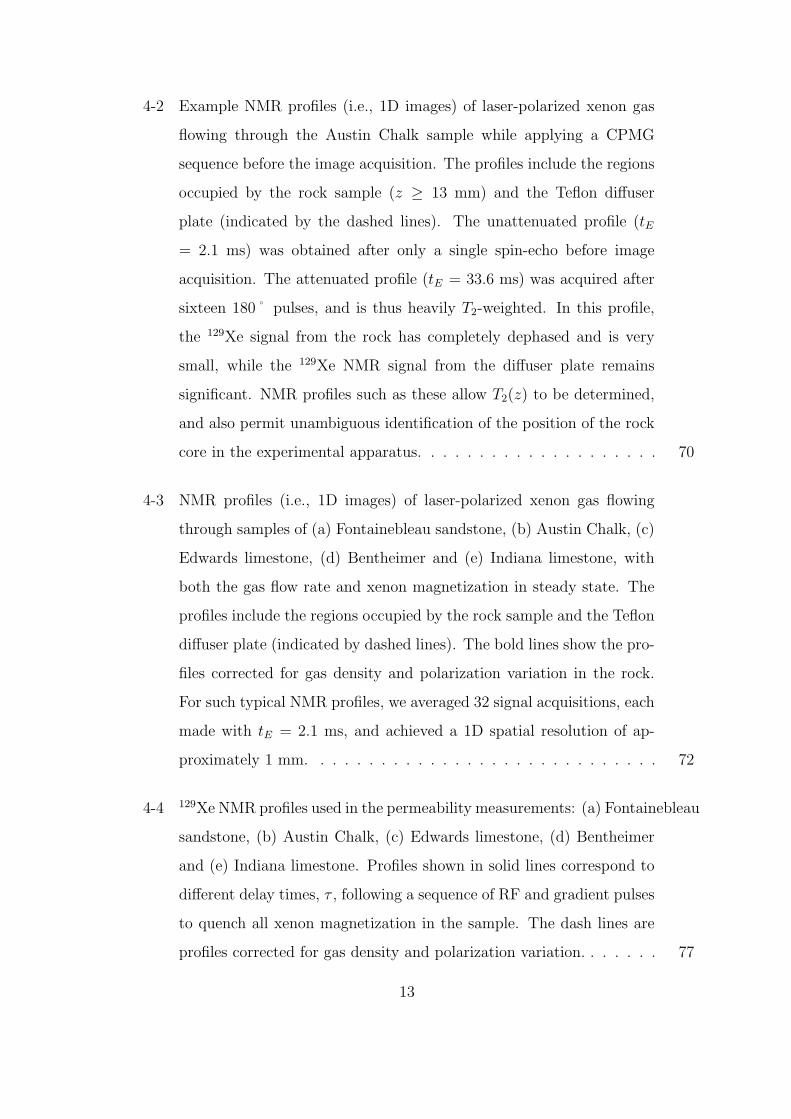
4-2 Example NMR profiles (i.e., 1D images) of laser-polarized xenon gas
flowing through the Austin Chalk sample while applying a CPMG
sequence before the image acquisition. The profiles include the regions
occupied by the rock sample (z ≥ 13 mm) and the Teflon diffuser
plate (indicated by the dashed lines). The unattenuated profile (tE
= 2.1 ms) was obtained after only a single spin-echo before image
acquisition. The attenuated profile (tE = 33.6 ms) was acquired after
sixteen 180˚ pulses, and is thus heavily T2-weighted. In this profile,
the 129Xe signal from the rock has completely dephased and is very
small, while the 129Xe NMR signal from the diffuser plate remains
significant. NMR profiles such as these allow T2(z) to be determined,
and also permit unambiguous identification of the position of the rock
core in the experimental apparatus. . . . . . . . . . . . . . . . . . . . 70
4-3 NMR profiles (i.e., 1D images) of laser-polarized xenon gas flowing
through samples of (a) Fontainebleau sandstone, (b) Austin Chalk, (c)
Edwards limestone, (d) Bentheimer and (e) Indiana limestone, with
both the gas flow rate and xenon magnetization in steady state. The
profiles include the regions occupied by the rock sample and the Teflon
diffuser plate (indicated by dashed lines). The bold lines show the pro-
files corrected for gas density and polarization variation in the rock.
For such typical NMR profiles, we averaged 32 signal acquisitions, each
made with tE = 2.1 ms, and achieved a 1D spatial resolution of ap-
proximately 1 mm. . . . . . . . . . . . . . . . . . . . . . . . . . . . . 72
4-4 129Xe NMR profiles used in the permeability measurements: (a) Fontainebleau
sandstone, (b) Austin Chalk, (c) Edwards limestone, (d) Bentheimer
and (e) Indiana limestone. Profiles shown in solid lines correspond to
different delay times, τ , following a sequence of RF and gradient pulses
to quench all xenon magnetization in the sample. The dash lines are
profiles corrected for gas density and polarization variation. . . . . . . 77
13

5-1 Five different fluidization regimes: fixed bed, homogeneous fluidiza-
tion, bubbling fluidization, slugging and pneumatic transport. Origi-
nally found in [1]. . . . . . . . . . . . . . . . . . . . . . . . . . . . . . 86
5-2 Geldart Classification of particles. Four groups of particles are iden-
tified according to their fluidization behaviors. dp is the size of the
particles, and ρp and ρf are density of the particles and gas, respectively. 89
5-3 Bubble shape and flow streamlines through around bubble. a. Flow
streamlines in and out of a bubble (for ub > uf ). The reference frame
is that where the bubble is static. b. Photograph of a bubble in a two-
dimensional bed, by Davidson and Hurrison in 1971 [2]. The arrows
indicate gas flow directions. . . . . . . . . . . . . . . . . . . . . . . . 94
5-4 Xenon exchange pathways in a bubbling fluidized bed, with all phases
included. The exchange between bubble and its encapsulating cloud is
the rate-limiting for gas flow from bubble to dense phase. . . . . . . . 97
5-5 Relative contributions to bubble-cloud exchange from the convective
and diffusive exchange mechanisms, calculated from Eqn. (5.8) with
Umf = 0.5 cm/s, and D = 3 mm2/s. Diffusive exchange predominates
when the bubble diameter is smaller than 30 cm. In our study, the
largest bubble size was 0.5 cm. As a result, we were always observing
exchange predominantly due to gas diffusion. . . . . . . . . . . . . . . 99
6-1 A schematic diagram of the Laser-polarized xenon - fluidized bed -
NMR apparatus. Narrow 1/8 inch ID Teflon tubing connected the
different sections of the apparatus, and provided the gas flow path.
The tubing length was approximately 2.5 m from the polarizer to the
sample, and 5 m from the sample to the mass flow controller. The
mass flow controller moderated the effect of the pump and determined
the gas flow in the particle bed. . . . . . . . . . . . . . . . . . . . . . 112
14

6-2 Complete assembly of the fluidized bed apparatus. a) Schematic draw-
ing; b) Photo of the actual assembly without the exhaust region in
place. The connections between the different plates are sealed by O-
rings. The bottom diffuser is mounted with a retention ring onto the
diffuser plate, while the top diffuser is glued to the column top plate.
At the bottom of the plate, the mounting of the apparatus onto the
NMR micro-imaging probe body is visible. . . . . . . . . . . . . . . . 114
6-3 Photos of the particles used in the fluidized-bed experiments, taken
with 100x microscope. a) Transparent glass beads sized between 45
and 70 µm, which results in them being classed as Geldart Group A
particles. The beads are highly spherical in shape. b) Opaque Al2O3
particles, sized between 75 and 104 µm, by passing through appropriate
sieves. These particles are classed as Geldart Group B and their shape
is highly irregular. . . . . . . . . . . . . . . . . . . . . . . . . . . . . 115
6-4 Alderman-Grant RF Coil. The 120◦ RF windows were chosen for opti-
mal field homogeneity. CT and CM are tuning and matching capacitors
which can be adjusted for optimal sensitivity at the 129Xe Lamor fre-
quency. . . . . . . . . . . . . . . . . . . . . . . . . . . . . . . . . . . . 116
6-5 2D slice-selective images of a cylindrical water phantom 3 mm in di-
ameter and 18 mm in length. a. X-Y plane image of a 1 mm thick
slice, with a resolution of 0.156 mm; b. Z-Y plane image of 2 mm-thick
slice, with a resolution of 0.469 mm. . . . . . . . . . . . . . . . . . . . 117
6-6 Hysteresis in bed expansion, measured as a function of gas flow rate.
Dry N2 gas was used in this measurement. The particles are the glass
beads with good sphericity, and are classed as Geldart Group A par-
ticles. Homogeneous fluidization was therefore observable for these
particles, with hysteresis apparent in this range of flow rates. . . . . . 119
15

6-7 Dependence of minimum-fluidization flow rate Umf on gas pressure.
The uncertainty on the measured flow rates is 0.1 sccm. N2 gas was
used to fluidize the glass beads. Data points were measured flow rates.
The solid line is a linear fit. . . . . . . . . . . . . . . . . . . . . . . . 120
6-8 Spectra of 129Xe in an Al2O3 particle bed, measured at 11 different
gas flow rates (Fourier Transform of the acquired free-induction decays
(FID) after a 90◦ hard pulse). The spectra were obtained by increasing
the gas flow rate from 15 to 125 sccm at gas pressure of 2.0 bar. The
narrow peak is believed to originate from the bubble phase. . . . . . . 123
6-9 Spectra obtained from 129Xe gas fluidizing a bed of Al2O3 particles.
a) The complete spectrum, acquired from a single RF pulse. b) The
spectrum acquired with a spin-echo sequence, with an echo time of 8
ms. The spin-echo spectrum clearly shows only the bubble peak, after
removal of the emulsion and adsorption signals due to spin decoherence
during the echo time. . . . . . . . . . . . . . . . . . . . . . . . . . . . 124
6-10 The NMR pulse sequence used in bubble-emulsion exchange rate mea-
surements. A π/2 hard RF pulse non-selectively flips spins into the
transverse plane. After application of a π pulse, a spin-echo is gener-
ated after time τ1. τ1 was chosen to be 8 ms, long enough for emulsion
and adsorption magnetizations to decohere. The bubble magnetization
is then stored along the z direction following the second π/2 pulse. Gas
exchange between the bubble and emulsion phases occurs during the
subsequent delay τ2. The third π/2 RF pulse then returns the remain-
ing magnetization back to the transverse plane, and the FID signal
is acquired after a delay time τ3 of 0.7 ms, which eliminates emulsion
and adsorption magnetization that may have migrated from bubbles
during τ2. Therefore, only 129Xe in the bubble phase contributes to the
FID signal, which can be used to acquire useful exchange data. . . . . 125
16

6-11 Two-phase flow model for gas flow in the bubble and emulsion phases.
Ab and Ae are cross-sectional area of bubble phase and the emulsion
phase, respectively. H is the height of the particle bed. U is the total
empty-tube gas flow velocity. εmf is the void fraction in the emulsion
phase. . . . . . . . . . . . . . . . . . . . . . . . . . . . . . . . . . . . 127
6-12 Measured particle bed expansion (a) and estimated bubble diameter
(b) as functions of gas flow rates. The size of the bubbles increases
monotonically with the flow rate. At 160 sccm, the bubble diameter
is greater than 60% of the column inner diameter, indicating that the
fluidization is approaching the slugging regime. This was confirmed by
visual inspection of the bed at that flow rate. . . . . . . . . . . . . . 129
6-13 Predicted bubble-emulsion exchange rate. Since 35 sccm was the point
where we started to observe a bubble peak in the 129Xe NMR spectra,
it was the lowest flow rate where bubble-emulsion exchange could be
measured. Thus the prediction curve does not extend to flow rates
below 30 sccm. The exchange rate is plotted on a logarithmic scale. . 130
6-14 Peak deconvolution in 129Xe spectra obtained from xenon gas fluidizing
Al2O3 particles. Deconvolution was achieved by fitting to three inde-
pendent Lorentzians. a) spectrum measured at flow rate of 35 sccm,
with a small bubble volume. b) spectrum at flow rate of 105 sccm,
with a large fraction of the gas in the bubble phase. The circles in the
two plots label the measured spectra, and the lines are fitting results. 131
6-15 Plot of the ratio of emulsion phase to adsorption phase volume, ψe/ψa
as a function of gas flow rate. ψe/ψa was seen to be independent of
flow rate, and determined to be 1.581 ± 0.044. The error bars were
estimated from the noise level in the spectra. . . . . . . . . . . . . . . 132
17

6-16 Plot of the dependence of ψb/ψa on gas flow rate, which is plotted here
on a logarithmic scale. The ratio steadily increases with flow rate,
consistent with the knowledge that bubble volume increases steadily
with gas flow rate. The error bars were estimated from the noise level
in the spectra. . . . . . . . . . . . . . . . . . . . . . . . . . . . . . . . 133
6-17 Decay of bubble magnetization at 15 different exchange times, τ2, and
two different flow rates: 60 and 40 sccm. The exponential fits yield
decay rates that were related to bubble-emulsion exchange. 256 signal-
averaging scans were used for each acquisition, and the resulting signals
coherently added to reduce variations in the bubble amplitude. The
delay times used in the sequence were: contrast delay time, τ1 = 8 ms,
exchange time, τ2, varied between 1 and 50 ms, pre-acquisition delay
τ3 = 0.7 ms. . . . . . . . . . . . . . . . . . . . . . . . . . . . . . . . . 135
6-18 Measurements of the bubble-emulsion exchange rate. The predicted
curve from Fig. 6-13 is included for comparison. 256 signal averaging
scans were summed in each measurement to reduce statistical errors.
The exchange rate is plotted on a logarithmic scale. . . . . . . . . . . 136
6-19 NMR pulse sequence used to measure the emulsion-adsorption ex-
change rate. Three π/2 selective pulses were used to rotate the ad-
sorption magnetization into the transverse plane repeatedly, so that
the magnetization balance between the two phases was disturbed. The
separation between any two soft-pulses is 1.0 ms, of the same order as
the transverse relaxation time of the adsorbed phase, T a2 . A delay time,
τ , was then used to allow exchange to occur between the adsorbed and
emulsion phases. Spins exchanging in from the emulsion phase retain
their high spin polarization. τ was varied in our experiments from 0.1
to 10 ms. Finally a non-selective π/2 RF pulse allowed sampling of
magnetization components in all phases, after exchange. . . . . . . . 138
18

6-20 (a) A single 129Xe spectrum measured at a gas flow rate of 60 sccm,
along with deconvoluted spectra for each component derived from fit-
ting the main spectra with three Lorentzians. (b) The derived spectra
for the adsorption peak only, after subtraction of the fitted bubble and
emulsion components measured at 16 different exchange times, τ . The
ripples around zero frequency are the result of imperfect subtraction
of the much larger bubble peak. The amplitude of the adsorption peak
increases slowly with the exchange time, τ , which was used to find the
exchange time. . . . . . . . . . . . . . . . . . . . . . . . . . . . . . . 140
6-21 The emulsion-adsorption exchange rate measured at nine different gas
flow rates. Each data point was result of exponential fitting of the
adsorption magnetization recovery to delay time, τ , as shown in Fig.
6-20 for 60 sccm. kea was then calculated with Eqn. (6.12). The
exchange rate is considered independent of flow rate. . . . . . . . . . 141
6-22 Xenon gas velocity distributions measured in two fluidization regimes.
50 µm glass beads were fluidized by laser-polarized xenon. Velocity
spectra were measured by the pulsed field gradient stimulated echo
technique, in which the gradient pulse duration, d = 1 ms, the flow en-
code time D = 10 - 1000 ms and the maximum gradient pulse strength
was 20 G/cm. a). Four different gas flow rates: 10, 16, 21 and 30
sccm were used, all of which ensured the particle bed was in the homo-
geneous fluidization regime. b). Similar measurements made at three
higher gas flow rates: 40, 50 and 75, corresponding to the bubbling flu-
idization regime. Also included is the data for 30 sccm, the transition
point between homogeneous and bubbling fluidization. The superficial
gas velocities corresponding to the flow rates are given in parentheses. 143
19
7-1 Recirculation of gas through a bubble. The circulating gas penetrates
the dense cloud around the bubble. The particles surrounding the
bubble are assumed to have negligible velocity compared to the bubble
rising velocity ub, according to Davidson’s bubble model. The thick
curve on the left shows the flow path of the recirculating gas which
moves with velocity ub − Umf , relative to the emulsion phase. . . . . 146
7-2 The expected bubble-emulsion exchange curve corresponding to the
presence or absence of adsorption. . . . . . . . . . . . . . . . . . . . . 148
7-3 kbe(1 + ψb
ψe+ψa) measured corresponding to two exchange behaviors. . . 149
7-4 The effectiveness of phase-cycling in removing the incoming bubble
magnetization during exchange time τ2. a) The time-dependence of
the bubble magnetization at 50 sccm measured with the phase-cycling.
b) Same measurement made at 50 sccm without phase-cycling. . . . . 150
7-5 The effect of the outflow of bubbles exiting the bed from the top. A
sudden decrease in bubble magnetization was found at a delay time of
100 ms. . . . . . . . . . . . . . . . . . . . . . . . . . . . . . . . . . . 151
A-1 Fluidized bed windbox design. . . . . . . . . . . . . . . . . . . . . . . 158
A-2 Fluidized bed bottom diffuser plate flange design. . . . . . . . . . . . 159
A-3 Fluidized bed column mounting flange design. . . . . . . . . . . . . . 160
A-4 Fluidized bed gas exhaust flange design. . . . . . . . . . . . . . . . . 161
B-1 A Second Fluidization Apparatus. . . . . . . . . . . . . . . . . . . . . 164
D-1 The pulse sequence. . . . . . . . . . . . . . . . . . . . . . . . . . . . . 168
20

List of Tables
2.1 Properties of Selected Spin-12
Nuclei . . . . . . . . . . . . . . . . . . . 29
2.2 Different Types of Relaxation Mechanisms . . . . . . . . . . . . . . . 34
2.3 Magnetic Susceptibility of Selected Substances . . . . . . . . . . . . . 38
4.1 Permeability and Effective Porosity Results . . . . . . . . . . . . . . . 78
5.1 Descriptions of Variables Used in Eqn. (5.12) . . . . . . . . . . . . . 105
7.1 Time Scales in the Fluidized Bed . . . . . . . . . . . . . . . . . . . . 152
C.1 Fluidized-Bed Parameters . . . . . . . . . . . . . . . . . . . . . . . . 166
D.1 Phase-Cycling in the Sequence . . . . . . . . . . . . . . . . . . . . . 168
21

22

Chapter 1
Introduction
This thesis describes the application of Nuclear Magnetic Resonance (NMR) tech-
niques to laser-polarized noble gases in order to study the dynamics of fluid flow in
porous and granular media. The results quantify several important parameters in the
two types of systems, revealing important structural and hydrodynamic information.
Porous and granular media are ubiquitous in nature, pharmaceuticals, as well as in-
dustrial fields such as oil-drilling and food processing. The complex fluid flow through
porous and granular media brings about many theoretically and experimentally chal-
lenging problems, with difficulties arising from the random arrangements and opaque
nature of the solid phase; and the large number of degrees of freedom which make
simulation difficult. Research on these materials has fundamental significance in both
physical and chemical sciences, in addition to its contributions to the improvements
of wide-ranging engineering practices.
The research concentrated on experimental investigations of the physical processes
by using gas-phase NMR. NMR has become a powerful, non-invasive probe of non-
metallic materials. The deep penetration of radio frequency energy (RF) into these
materials, which contain nuclear spins capable of resonant absorptions and emissions
at specific frequencies in the presence of an external magnetic field, permits this
study of materials in different physical and chemical states. The resultant signals
are rich with information relevant to different fields of study, and the technology has
spread from physics to chemistry, material research, bioscience and clinical diagnosis.
23

Researchers continue to expand the scope of NMR to new fields and applications.
Gas-phase NMR has traditionally suffered from poor signal-to-noise ratio, mostly
due to the low spin density of gases. The development of the spin-exchange optical
pumping technique, which enhances the spin polarization of certain noble gases by
up to 5 orders of magnitude, can provide gas-phase spin magnetization comparable to
that of the liquid phase in magnetic fields ∼ 1 T. The pumping process involves the
indirect transfer of photon polarization to the nuclear spins of the noble gas species,
and is most efficient in 129Xe and 3He, which have a nuclear spin number of 12. The
laser-polarization technique, first pioneered in 1950’s [3], has matured and platforms
capable of delivering large volumes of laser-polarized gas are now available. We
developed a home-built polarization system for polarizing natural-abundance xenon
and providing a continuous flow of laser-polarized gas into the NMR samples located
in the NMR magnet.
Chapter 2 summerizes the basics of the NMR technique. Starting with a descrip-
tion of the quantum-mechanical picture of a single nuclear spin in the presence of
a magnetic field, the chapter lists important aspects of NMR experiments, includ-
ing chemical shifts, magnetic susceptibility and nuclear relaxation phenomena - due
to the interactions of the spin system with its environment, as well as among the
spins themselves. This chapter also covers two established applications of NMR, in
which the spatial density maps of a material and information about the dynamic
displacement of spins are obtained.
Chapter 3 covers both the principles underlying the spin-exchange optical pump-
ing process and the specifics in applying NMR techniques to laser-polarized noble
gases. The two stages of transferring photon polarization to nuclear spins are dis-
cussed, together with primary measures for optimizing the pumping efficiency. This
chapter also explains differences between laser-polarized noble gas NMR and its con-
ventional thermally-spin-polarized counterpart, followed by several examples demon-
strating special modifications necessary in such experiments.
In Chapter 4, the methodology and experimental details for simultaneously mea-
suring gas permeability and effective porosity of reservoir rocks are described. We
24

introduce these two important parameters, which characterize the fluid transport
processes in porous media; relate the flow properties to each parameter based on the
fluid dynamics describing flow in porous media; present the experimental schemes
and measurement results; and compare the results to those available from established
methods.
Chapters 5 through 7 present the model, experiments, results, and relevant dis-
cussions on experimental studies of gas dynamics in a gas-fluidized bed.
Chapter 5 introduces the basic aspects of a system of gas-fluidized granular par-
ticles and covers the definition and importance of the exchange behavior in such a
system. The first half of this chapter describes the different fluidization regimes, the
classification of particles, and two distinct exchange behaviors. In addition, the chap-
ter discusses in detail a model governing the dynamics of different phases in terms of
nuclear spin magnetizations, providing a context for the experiment design and data
analysis.
Chapter 6 details the measurement of gas exchange rates experimentally by using
specifically designed NMR methods. The description of the experimental apparatus
includes the design of the fluidized bed setup, choice of particles and design of the
RF probe. Also discussed are the methods used to obtain contrast between different
phases in the fluidized bed, as well as the NMR pulse sequences designed to perform
the measurement. This chapter concludes by presenting the experimental data and
the measurement results.
Chapter 7 re-evaluates the assumptions made in building the experimental model
for the fluidized-bed study by using the quantitative estimations and actual experi-
mental results. This chapter also covers the significance of this research in the con-
text of the granular media field, together with the universality and limitations of the
method.
25

26

Chapter 2
Nuclear Magnetic Resonance
2.1 Introduction
Nuclear magnetic resonance (NMR) has been one of the most successful technologies
in modern science. The beauty of NMR lies in the fact that it is sensitive to spins
hosted by nuclei of size 10−15 m, and is able to effectively manipulate these spins to
yield a wide variety of information. The dynamics of a single nuclear spin are affected
by the spin’s local magnetic field, which is generated by a combination of effects from
nearby nuclei, electrons, or external magnets. The resultant NMR signals are rich
with structural and dynamical information on molecules or atoms in objects ranging
in size from a rock pore or biological cell up to human brains. In only a few decades
of development, this technology has spread from physics, to chemistry, to material
research, bioscience and clinical diagnosis [4].
Researchers are still extending the technology to dramatically different new fields
such as implementation of quantum computation, soft-matter physics, and cellular
metabolism.
2.2 History
In 1945, the magnetic resonance phenomenon was first observed by two independent
groups, led by Ed Purcell (Harvard University) and Felix Bloch (Stanford Univer-
27

sity), who shared the Nobel Prize in physics in 1950. The availability of commercial
magnets in the late 1950’s significantly promoted development of both NMR the-
ory and technology. The year 1966 saw a major breakthrough, when Richard Ernst
discovered that the sensitivity of spectra could be enhanced ∼ 100 fold if the slow
frequency sweep was replaced by intense radiofrequency (RF) pulses. He went further
to introduce the Fourier Transform into data analysis, from which different frequency
components were immediately separable. This revolutionary work, along with seminal
developments in two-dimensional NMR spectroscopy, earned him the Nobel Prize for
chemistry in 1991. In the decades after 1970, the improvements in super-conducting
magnets and concurrent advances of computer technology lead to the rapid develop-
ment of experimental techniques involving multiple frequency dimensions. Another
milestone in the history of magnetic resonance technology occurred in 1973, with the
application of a linear field gradient to generate frequency encoding with spatial de-
pendence, which opened the door for the enormously successful magnetic resonance
imaging technologies, now known as MRI. Paul Lauterbur and Peter Mansfield shared
the 2003 Nobel Prize in Physiology or Medicine for their original work in the building
foundations for MRI.
2.3 Spin Dynamics
Spin is an intrinsic quantum-mechanical property of a nucleus, and its measure is
determined by the number of protons and neutrons existing in each nucleus. The
majority of NMR studies utilize spin-1/2 nuclei because of the ease in manipulation,
observation and analysis. The magnetic moment ~µ of a nucleus is proportional to its
spin ~J by
~µ = γ ~J, (2.1)
where γ is the gyromagnetic ratio of the nucleus. Table 2.1 lists properties of several
nuclear species commonly used.
NMR technology has been mostly applied in the liquid or soft-condensed matter
28

Table 2.1: Properties of Selected Spin-12
Nuclei
Lamor Natural MagneticFrequency Abundance Moment
Isotope (MHz/T) (%) (µN)1H 42.577 99.984 2.792703He 32.434 1.3×10⁻⁴ -2.127413C 10.705 1.108 0.70216
129Xe 11.78 26.24 -0.7726
phase, with 1H being the most common “working nucleus”, as it is ubiquitously found
in aqueous, organic and biological samples. Being gaseous at room temperature,
3He and 129Xe were not favored as candidates since they contributed very low NMR
signal intensity due to their significantly lower spin density. However, gas-phase NMR
studies on these species are made possible by laser-polarizing, or enhancing the spin
polarization of the gas beforehand. Additionally, Xe atoms have a large electron
cloud which easily deforms and interacts with other atoms. As a result, 129Xe spins
are very sensitive to their chemical environment, and a chemical shift range as large
as 300 ppm has been observed [5, 6]. Different 129Xe resonances have hence been used
to label different chemical or physical states in the study of transport and exchange
behavior [7, 8].
When a single spin-1/2 nucleus is placed in a static magnetic field B0, the Hamil-
tonian describing the Zeeman interaction between the spin and field is
H = −~µ · ~B0 = µzB0, (2.2)
if we use a laboratory coordinate frame such that the z-axis is along the applied
magnetic field direction. The interaction breaks the nuclear energy-level degeneracy
for Iz, and the Hamiltonian H results in two levels ±γ~B0/2, dependent on whether
the spin is parallel (Iz = ~/2) or anti-parallel (Iz = −~/2) to the B0 direction. The
energy difference between the two levels is γ~B0, with lower energy in ~/2 state. The
resonance or transition frequency ω between the two levels, also known as the Larmor
29

frequency, is
ω = γB0. (2.3)
and the equation of motion for the spin state is given by the Schrodinger equation
−i~∂|ψ〉∂t
= H|ψ〉. (2.4)
In practice, we always look at a sample with a large number (1019) of spins of
the same species, each of which may occupy different states. The system may be
conveniently described if we introduce the density matrix
ρ =∑
ψ
pψ|ψ〉〈ψ|, (2.5)
where |ψ〉 is one of the spin states, which are usually chosen to be the eigenstates of
Hamiltonian given in Eqn. (2.2). pψ is the probability of finding a spin in the state
|ψ〉. Measurement of spin on the system yields an ensemble average∑ψ
pψ〈ψ| ~J |ψ〉 or
simply Tr(ρ ~J). The dynamics of the density matrix follows Liouville equation
i~∂ρ
∂t= [H, ρ]. (2.6)
The equation of motion for an ensemble average with magnetic moment ~µ is then
given by
∂〈~µ〉∂t
=1
i~Tr([H, ρ]~µ) =
γ
i~Tr(ρ[ ~J, H]) = γ2B0〈 ~J〉 × z = 〈~µ〉 × γ ~B0. (2.7)
This is equivalent to the classical description for the movement of a magnetic
moment in an external field [9]. Therefore, it is justified to treat the spin ensemble
classically, if we ignore the interaction between the spins, which is not included in
Eqn. (2.2) [10]. The ensemble average of the magnet moment may be simply depicted
as a vector, with its time-dependence given by Eqn. (2.7).
30

Under thermal equilibrium, the spin populations on the two energy levels are
determined by Boltzmann distribution
n± =e±
γB0~2kT
eγB0~2kT + e−
γB0~2kT
, (2.8)
and the spin polarization of the system is
p = n+ − n− =e
γB0~2kT − e−
γB0~2kT
eγB0~2kT + e−
γB0~2kT
. (2.9)
Typically the energy splitting is much smaller than the thermal energy (γB0~2kT
=
1.6 × 10⁻⁵ for B0 = 4.7 T and at room temperature); hence p ≈ γB0~2kT
is a good
approximation under most circumstances. The nuclear magnetization in a sample
placed in an external field B0 is defined as the total net magnetic moment per unit
volume, or the single spin moment multiplied by the polarization and atom number
density N :
M0 =~2γpN =
γ2~2NB0
4kT. (2.10)
This is the magnetization along the B0 field direction at thermal equilibrium, and is
also the state of the spin system where all liquid and solid-phase magnetic resonance
experiments start. Magnetization at any other instant is given by ~M = N〈~µ〉, and
its time-dependence is governed by the famous Bloch equation [11],
d ~M
dt= γ ~M × ~B0 − Mz −M0
T1
z − Mxx + Myy
T2
. (2.11)
T1 and T2 are included to phenomenologically account for longitudinal and transverse
spin relaxations respectively.
2.4 Relaxation
Assuming a homogeneous externally-applied field B0, relaxation of an ensemble’s
spin polarization is caused by local magnetic fields experienced by the nuclear spins,
31

which arise from interactions between the spins and their surrounding environments,
including electrons and other nuclei, in the form of dipolar or other higher order
interactions. Due to random motions, the local field is not static, but rather undergoes
large fluctuations in both magnitude and orientation. Typical examples of these
motions include rotation and translation of molecules that bind the nuclei together.
Not only the strength but also the rate of the fluctuations significantly affect the spin
behavior, which manifests itself as the relaxation parameters: the longitudinal and
transverse relaxation rates.
2.4.1 Longitudinal Relaxation T1
Suppose a spin ensemble, or NMR sample, is originally placed at zero field. The net
magnetization is zero because there is no energy split and the spins assume no pref-
erence in their orientation. If a magnetic field ~B0 is turned on at t = 0 and Zeeman
split generated, the nuclear spins tend to be rotated towards an equilibrium Boltz-
mann distribution of populations. The process for the system to reach equilibrium, in
which the spin populations satisfy Eqn. (2.8), is called the longitudinal relaxation. If
the relaxation of spin magnetization follows a single exponential curve, we designate
its time constant as T1. Longitudinal relaxation is also referred to as spin-lattice
or spin-polarization relaxation, as the process involves energy exchange between the
spins and their surrounding thermal environment.
T1 relaxation is the result of spins reversing (flipping) their orientation, with ab-
sorption or emission of an amount of energy equal to γ~B0, the energy difference
between the two Zeeman levels. This corresponds to a frequency value of ω0 = γB0,
or the Larmor frequency. If the fluctuation frequency of a local magnetic field has
a frequency component at ω0, then this local field contributes to the longitudinal
relaxation. The larger the magnitude of field fluctuations at ω0, the shorter the T1
relaxation time.
T1 is measured by observing the return of the spin system to equilibrium after it
is initially disturbed by an RF pulse. As an example, we next describe the inversion-
recovery method for measuring T1. A 180◦ RF pulse may be used to invert the
32

spin magnetization from +z direction (equilibrium state) to −z direction. The effect
of T1 relaxation is to gradually restore magnetization M to +z direction, with a
time-dependence given by M = M0(1 − 2 exp(−t/T1)) where M0 is the magnitude
of magnetization at thermal equilibrium. After a delay time t following the 180◦
pulse, M is measured by flipping the spins onto the transverse plane with a 90◦ pulse
and then acquiring the free induction decay (FID). Multiple such measurements are
needed with different lengths of the delay time t, in order to get complete information
on the time-dependence of magnetization, from which T1 value is available by fitting
the data to an exponential.
2.4.2 Transverse Relaxation T2
It is routine to rotate spin magnetization from the longitudinal direction onto the
transverse plane, to initiate an NMR experiment. These spins start with the same
phase and undergo coherent Larmor precession, but dephase gradually because the
spin-spin interactions result in different local magnetic fields for different spins, even in
a perfectly homogenous external field. Phase coherence is lost over the characteristic
timescale T2 and the transverse magnetization diminish to zero. Various names have
been used to refer to this phenomenon: transverse relaxation, decoherence spin-spin
relaxation and T2 relaxation.
In a heterogeneous external magnetic field, such as that due to susceptibility
contrast between different materials or an intentionally applied imaging gradients,
the decay time constant for the transverse magnetization is shorter than T2 and
is known as T ∗2 . The spin-echo is a powerful NMR technique invented to regain
spin coherence lost due to invariant external field inhomogeneities, by applying an
appropriately timed phase-inverting 180◦ RF pulse [12]. The Carr-Purcell sequence
extends this idea by using multiple 180◦ pulses, and the resultant echo train forms
an envelope that decays with the time constant T2. Spin dephasing caused by T2
relaxation is inherently random and cannot be refocused with RF pulses1, which is
1This applies to interactions between “like” spins of the same nuclear species. It is possible torefocus coherence loss due to invariant interactions between different types of nuclear spins.
33

Table 2.2: Different Types of Relaxation Mechanisms
Relaxation Mechanism Description
Dipole-Dipole Relaxation Interaction of the spin with the magnetic fieldgenerated by another nearby nuclear spin. Mostpopular for spin 1/2 nuclei.
Quadrupolar Relaxation Relaxation due to the asymmetricelectric field around a quadrupolar nucleus,usually from a spin of half integer butlarger than 1. e.g. 27Al, 59Co.
Chemical Shift Anisotropy The value of chemical shift varies as a function
of molecule orientation with respect to ~B0 field.e.g. 31P and solid state samples.
Paramagnetic Relaxation The large fluctuating field generated by unpairedelectrons in paramagnetic materials, such as Gd2+.
Spin Rotation Relaxation Coupling of spin and angular momentum in abi-molecule collision. Usually occurs in gas-phasesystems.
Scalar Relaxation Interaction between two nuclei mediatedby electrons, also called J-coupling.
usually called homogeneous broadening of the NMR spectrum, while inhomogeneous
broadening refers to recoverable (T ∗2 ) coherence loss.
2.4.3 Relaxation Mechanisms and Quantum-Mechanical Re-
sults
Spin relaxation originates from spatially varying local fields, modulated by molecular
motions. Many different types of interactions can lead to these field variations, and
hence to spin relaxation. Different relaxation mechanisms are listed in Table 2.2.
Of all the relaxation mechanisms, dipole-dipole relaxation is the most important
in liquid state NMR with spin-1/2 nuclei.
The relaxation problem can be treated quantum-mechanically by solving the Liou-
ville equation (2.6) describing the dynamics of the density matrix for the spin system.
The Hamiltonian of the system is the Zeeman energy plus interaction terms, which
is typically decomposed into a superposition of spin operators with time-dependent
34

10-12 10-11 10-10 10-9 10-8 10-710-3
Correlation Time τ (s)
Rela
xati
on T
imes
(s)
10-2
10-1
100
101
102
103
c
T
T2
1
ω τ = 1 c0
Figure 2-1: Dependence of relaxation times on correlation time τc. Two differentmotion regimes are identified.
prefactors F (t) that describe the molecular rotational and translational motions. The
time-varying modulations are best described by the spectral density function, J(ω),
the Fourier transform of the auto-correlation function of F (t), which describes the
intensity of the motion-modulated interactions in the frequency domain. For the
dipole-dipole interactions in a spin-1/2 system, the calculated relaxation rates are
linearly related to values of J(ω) at discrete frequencies [13]:
1
T1
= J(ω0) + 4J(2ω0), (2.12)
1
T2
=3
2J(0) +
5
2J(ω0) + J(2ω0).
The above two equations clearly demonstrate that longitudinal relaxation is sensi-
tive to motions with large spectral components at the Lamor frequency and harmonics
of the spins in question, while transverse relaxation is also dependent on the static
field. Assuming the auto-correlation function of F (t) is an exponential with respect
to time, the spectral density function can then be written as [13]
35

J(ω) =2τc
1 + ω2τ 2c
, (2.13)
where τc is the interaction correlation time, i.e., the duration between two molecular
configurations; e.g., tumbling or translational time. For a very large τc so that ω0τc À1, J(ω0) ≈ 0 and J(0) ≈ τc; while in the case that ωτc ¿ 1, J(ω0) ≈ J(0) = 2τc. A
maximum of J(ω0) is found when τc = 1/ω0. Fig. 2-1 shows typical T1 and T2 values
as functions of τc. In liquid or gas systems with fast molecular or atomic motions,
ωτc ¿ 1 is easily satisfied and we have T1 ' T2, and the spectral line is very narrow.
On the other hand, motions are very slow in solids, and T2 has hence been observed
to be much shorter than T1. Moreover, T2 ≤ T1 in all circumstances.
This straightforward formalism explains a wide array of spin relaxation phenom-
ena very successfully. It may be applied in many situations where the dipole-dipole
interactions are the dominating contributor to relaxation.
2.5 Chemical Shift
A nuclear spin interacts with the spin and angular momentum of nearby nuclei and
their electron clouds, making NMR a sensitive tool for probing its local chemical
environment. A nuclear spin surrounded by electrons experiences magnetic shielding
in an external field due to the rearrangement of the electron cloud. This leads to slight
changes in the spin’s Larmor frequency, or a ”chemical shift”, where the magnitude
of shift is highly dependent on the type of atoms the nucleus is bonded to or in close
proximity to. Detailed chemical shift measurements have been used to determine the
structure of organic molecules. In chemical shift imaging (CSI), separate NMR images
of a single sample may be acquired from protons in different chemical environments,
providing spatial distribution of different chemical components.
129Xe is well-known for sensitivity to its chemical environment due to the large
xenon atomic number and hence its very large electron cloud, which is readily per-
turbed by external magnetic fields, and hence very large 129Xe chemical shifts have
been observed in different situations. For example, a spectrum of 129Xe dissolved
36

into blood showed a chemical shift of 200 p.p.m [14] up field from the gas peak while
liquid and solid xenon have chemical shift of 250 and 300 p.p.m. respectively from the
gas peak [15]. Laser-polarized 129Xe is well suited as a tracer of blood flow, allowing
the detection of exchange and transport phenomena between gaseous and dissolved
phases in the lung, where gas exchange occurs [4].
2.6 Susceptibility-Induced Shift and Line Broad-
ening
When placed in an external field, B0, any homogeneous material is magnetically
affected such that the resulting actual field strength inside the material is given by
B = (1 + χ)B0, (2.14)
where χ is the material’s magnetic susceptibility. χ for different categories of materials
varies in both amplitude and sign, with most substances being either paramagnetic
(χ > 0) or diamagnetic (χ < 0). Paramagnetism arises from the net atomic an-
gular momentum due to unpaired electrons in partially filled orbits. χ values for
paramagnetic materials are therefore positive and can be very large. Conversely, dia-
magnetism, which is found in most compounds, is the result of small disturbances of
filled electron orbits, and as such has the same origin as the chemical shift2. Dia-
magnetic materials have negative χ values, since the effect of the orbit disturbance
tends to cancel the external field. The absolute value of χ in diamagnetic materi-
als is typically 2 - 4 orders smaller than that for paramagnetic materials. Table 2.3
lists values of susceptibility, χ, multiplied by molar volume Vm (volume per mole) for
several substances often used in NMR experiments.
χ as defined in Eqn. (2.14), is the volume susceptibility, and is proportional to the
density for a given type of material. The magnetic susceptibility for solids and liquids
2The major difference between chemical shift and susceptibility is in the range of interactions.Chemical shift affects the nucleus in the same molecule while field due to susceptibility extends faroutside the molecule.
37

Table 2.3: Magnetic Susceptibility of Selected Substances
Material Formula χVm(×10−6 cm3/mol)Helium He -2.02Carbon (graphite) C -6.0Water H2O -12.63Silicon Oxide SiO2 -29.6Sodium Chloride NaCl -30.2Aluminum oxide Al2O3 -37Xenon Xe -45.5Copper chloride CuCl2 +1080Gadolinium Chloride GdCl3 +27930
is hence three orders of magnitude larger than that for gases. In porous and granular
media where gas and solid phases coexist in the same external field, there exist large
variations in magnetic susceptibility. The susceptibility variations are especially high
at the boundary between a solid and gas phase. The local magnetic field ~Bl in the
void space surrounding the solid grains or particles can be considered to be due to
susceptibility in the solid phase, if the much smaller counterpart from gas phase is
neglected. ~Bl is highly heterogeneous, with direction and magnitude dependent on
both the size and shape of particles, as well as their packing conditions. Audoly et
al. found that in a tight random pack of spherical beads, the local field at a spatial
point that is scaled by the bead size d (i.e., ~rd), is independent of d, and the field
gradient decreases inverse linearly with particle size [16]. The case of irregularly
shaped particles is very complicated and the field distribution is much broader.
The z-projection of the local field is important when studying fluid flow in porous
and granular media using NMR techniques, and is characterized by its average value
Blz and variation (∆Bl
z)2. Bl
z affects the average Lamor frequency and determines
the shift of the center of the spectral peaks, while
√(∆Bl
z)2 is the broadness of the
field distribution and is related to the peak line width.
38

2.7 Diffusion and Measurement with NMR
2.8 Diffusion
Diffusion is a process arising from the random Brownian motions of molecules driven
by thermal energy. Frequent collisions with neighbors randomize the molecular (or
atomic) velocity, and as such the trajectory followed by each molecule may be de-
scribed by a random walk. The signature of diffusion is that the r.m.s displacement
of molecules is linearly dependent on time, with a proportionality constant named
the self-diffusion coefficient. The macroscopic manifestation of diffusion is intermix-
ing and transport of mobile substances. The random motion of the molecule makes
this process non-reversible, and therefore in NMR experiments with fluids, the result
is a spin magnetization pattern that can not be recovered by any means. If spa-
tial variations exist in concentration of the diffusive substance, the diffusion process
tends to induce a net flux of molecules towards the region of lower concentration.
The magnitude of flux is related to the concentration gradient in a similar manner
to other gradient-induced flows, such as Darcy’s Law for flow through porous media
and Fourier’s Law for heat transfer. The diffusion coefficient D is defined in Fick’s
First Law [17],
J = −D∇c, (2.15)
where c is the molecular concentration, and J is the molecular flux. Diffusion is
prominent and fast in gases and liquids, but ionic diffusion in solid crystals also has
been observed. At atmospheric pressure and room temperature, typical gas diffusion
coefficients are on the order of 10−6 m2/s, which is three orders larger than that in
most liquids and 25 orders larger than solid-phase diffusion.
According to the continuity condition, at each spatial point, the material deriva-
tive of concentration should be equal the net incoming flux. We therefore have Fick’s
Second Law
39

∂c
∂t= D∇2c. (2.16)
in which a spatially homogeneous diffusion coefficient is assumed.
In NMR and MRI of liquids or gases, the diffusion phenomenon has significant
implications. It adversely causes NMR signal attenuation due to molecular diffusion
in the presence of a background field gradients by B0 inhomogeneities or magnetic
susceptibility contrast. Conversely, diffusive attenuation of NMR signal also yields
useful information about molecular transport, fluid properties and the geometry of
solid boundaries, if appropriate NMR methods are used to perform the measurements.
2.8.1 NMR Technique for Measuring Diffusion and Flow
In order to study transport phenomenon with NMR, a quantity called the propagator
is introduced, which is the ensemble-averaged probability for a molecule to displace a
distance ~R during time t. We denote the propagator by P (~R, t), which is effectively
another presentation of the fluid concentration and its dynamics following Fick’s Law
[18].
∂P (~R, t)
∂t+ ~u · ∇P (~R, t) = D∇2P (~R, t). (2.17)
Here D is the diffusion coefficient. Assuming a constant coherent flow velocity ~u in a
unconstrained system, we have the following solution to Eqn. (2.17),
P (~R, t) = (4πDt)−32 e−
(~R−~ut)2
4Dt , (2.18)
which is a gaussian function with the center moving at velocity ~u and the width ever
expanding.
The Pulsed-Gradient Spin Echo (PGSE) sequence has been successfully applied in
measuring molecule displacement, by applying a spatial modulation to the magneti-
zation and then observing the time-dependence of the modulation [19]. The sequence
is schematically shown in Fig. 2-2.
40

2
π
RF
τ
π
∆
ECHO
G δ g
Figure 2-2: PGSE pulse sequence for spin-transport measurement. Two magnetic fieldgradient pulses are used in combination with 90-180- spin-echo RF pulse sequence.The width of the two gradient pulses is δ, and the separation between them is 4.The gradient strength ~g is defined as ~g = ∂Bz
∂x~i + ∂Bz
∂y~j + ∂Bz
∂z~k.
Two gradient pulses with width of δ are placed after 90◦ and 180◦ RF pulses,
which produce a spin-echo, to generate and remove the spatial modulation of spin
magnetization. If a spin is located at ~r at the time of the first gradient pulse, its
transverse moment vector accumulate a phase factor φ = ~q · ~r, in which ~q = γδ~g. φ
is inverted after the 180◦ RF pulse. Suppose the spin moves to ~r′ at the time of the
second gradient pulse, after which the net phase will be φ = ~q · ~r′ − ~q · ~r = ~q · ~R,
where ~R is the displacement of the spin during 4. Since what we observe is the
ensemble-averaged displacement made by different spins, the echo amplitude may be
written as
E(~q) =
∫P (~R,4)ei~q·~Rd~R, (2.19)
which represents the signal strength at the center of echo, and is equivalent to the
inverse Fourier transform of the propagator P (~R,4). If multiple scans are made with
incremental ~q values, we may Fourier transform the echo amplitude with respect to
~q to get the transport propagator,
P (~R,4) =
∫E(~q)e−i~q·~Rd~q. (2.20)
The PGSE experiment has provided an innovative approach for probing fluid
transport either in bulk flow or through porous and granular media. We will see
41
examples of propagator measurement on gas flow through a fluidized bed in Chapter
6.
The above formulation does not take into account T2 relaxation, which exists
whenever manipulation of the transverse magnetization is performed. But its effect
is simply an additional multiplication factor of e− tE
T2 , where tE is the echo time, or
duration between the 90◦ pulse and the time of the echo center.
There is an upper limit on the measurable molecule displacement. Since ~q · ~R may
not exceed the maximum phase angle 2π, and the maximum measurable displacement
along the gradient direction is
R ≤ 2π
γδgm
, (2.21)
in which gm is the maximum strength of gradient pulses applied in the measurement.
If Eqn. (2.21) is not satisfied, phase-wrapping occurs yielding incorrect displacement
values.
2.9 Imaging
2.9.1 Principle
In the presence of an applied linear field gradient, the magnetic field strength at
spatial coordinate ~r varies according to
B(~r) = B0 + ~G · ~r, (2.22)
where ~G = ∇Bz is the field gradient. The resonance frequency is hence also dependent
on ~r. In a frame that rotates at the Lamor frequency ω0 = γB0, spins with spatial
coordinate ~r then rotate at a frequency of
ω(~r) = γ ~G · ~r. (2.23)
The NMR signal is from all spins in the sample covered by the RF coil, and may
42

thus be written as, aside from a proportionality constant,
S(~k) =
∫∫∫ρ(~r)ei~k·~rd3~r, (2.24)
where ~k = γ ~Gt, and ρ(~r) is the spatial distribution of spins in the sample. ~k has
the units of the reciprocal space. We then have a Fourier-conjugate relationship, now
between the NMR signal and the static spatial spin distribution, and a map of spin
density is provided by
ρ(~r) =
∫∫∫S(~k)ei~k·~rd3~k. (2.25)
In magnetic resonance imaging (MRI) experiments, we use different field gradients
to vary the value of the three dimensional vector ~k, and thus to span the so-called
k-space. Molecule density information in real space are retrieved by Fourier transfor-
mation on the acquired NMR data. Due to the ubiquity of protons in nature, MRI is
now a powerful and well-developed tool widely applied in bioscience, clinical diagnosis
and many industrial fields.
2.9.2 One-Dimensional Imaging
One-dimensional imaging, also called the 1D profile measurement, is performed by
scanning k-space only along a single direction. The field gradient applied is G =
dBz/dx~i if a spin density map along the x-direction is desired, which is related to the
NMR signal S(k) by
ρ(x) =
∫S(k)eikxdk, (2.26)
where k = γGt. This measurement could be simply implemented by applying a
90 degree pulse, and then immediately turning on the gradient and starting data
acquisition of the NMR FID. However, such image data start from t = 0 and are not
symmetric along the k-axis. Its Fourier transform hence contains both absorptive and
dispersive parts, and the data needs to be phased to remove the dispersive part before
43

2
π
RF
G
π
ECHO
G G
x
2ττ
x x
Figure 2-3: Pulse sequence for one-dimensional image acquisition. Read gradient isapplied in a standard spin-echo sequence.
reconstructing the image. To circumvent this inconvenience, a pulse sequence based
on the spin echo has been designed, by using a refocusing process in the first half of
the echo signal as the negative-time part so that the whole signal is symmetrical in
k-space. An additional benefit of using the spin echo instead of FID for imaging is
that the amount of signal is doubled, which helps to improve the signal-to-noise ratio.
Fig. 2-3 shows a typical sequence for measuring one-dimensional images.
The first gradient pulse shifts the starting point in k-space to k = −km = −γGτ ,
while the second gradient pulse, called the read gradient since acquisition takes place
at the same time, sweep k-space from −km to km. Then Eqn. (2.26) can be used to
reconstruct the one-dimensional image, by using an appropriate range of k values as
integration limits. The field of view for this image acquisition is determined by
FOV =SW
γG, (2.27)
where SW is the spectral width, equivalent to the sampling frequency for digitization.
The optimal resolution in the resulting image is
RES =SW
γGN, (2.28)
where N is the number of points used for digitization. The actual resolution might be
worse than that expected in the above equation, with the two primary reasons being
T2 relaxation and molecule diffusion during the acquisition. T2 relaxation results in a
44

RF
G
π
ECHO
G Gx
2ττ
G y
x x
yG
G z
π
2
Figure 2-4: Pulse sequence for two-dimensional slice selective image acquisition. Alonger, SINC-shaped pulse with reduced power is used to selectively excite a certainslice within the sample. Phase-encoding gradient Gy and frequency-encoding gradientGx scan the entire k-space.
finite spectrum linewidth equal to 1/πT2, and no features narrower than that could be
identified in the frequency domain. Therefore, T2-limited resolution may be estimated
to be 1/πT2γG. Molecular diffusion in the presence of field gradients will cause decay
of the transverse magnetization, which equivalently broadens the line by an amount
[18]
∆fD = 0.6(γ2G2D/3)13 , (2.29)
and results in a resolution no better than ∆fD/γG.
2.9.3 Two-Dimensional Imaging
Figure 2-4 shows a typical pulse sequence for obtaining slice-selective two-dimensional
images. A SINC-shaped soft RF pulse is used to excite spins only in a particular slice,
whose spatial location and thickness are determined by the bandwidth and central
frequency of the pulse, together with a simultaneously applied z-gradient Gz. The
45

kx
ky
Start
Figure 2-5: Trajectory followed by the two-dimensional image acquisition to scank-space.
result of the selection is a square profile along the z direction since the shape of the
excited magnetization is the the Fourier transform of the pulse shape [18]. Phase-
encoding is performed by adding a Gy gradient before the 180◦-pulse. Multiple values
of Gy are needed in order to sweep through the two-dimensional k-space completely.
Fig. 2-5 shows the trajectory for sweeping through k-space, if the pulse sequence
shown in 2-4 is applied.
46

Chapter 3
NMR with Laser-Polarized 129Xe
Gas
3.1 Introduction
Traditionally, gas-phase NMR has been difficult primarily because the typical gas
density is three orders smaller than that in the liquid phase. Even though the spin
polarization achievable at thermal equilibrium in a tesla-scale magnetic field is com-
parable for gases and liquids, the magnetization - effectively the product of density
and polarization - is a thousand times weaker. Therefore, the signal-to-noise ratio
(SNR) is extremely poor for gas-phase NMR, and tens of thousands of signal averages
are necessary to compensate for the low signal intensity.
This problem has been mitigated by the development of spin-exchange optical
pumping, in which the polarization of noble gas species, typically 3He and 129Xe, can
be enhanced by up to a factor of 105. The implementation and operation of the optical
pumping apparatus is well developed now, and the technology is widely applied in
biology and medical studies, as well as in material science.
For example, laser-polarized (i.e., hyperpolarized) 129Xe and 3He has been applied
to make pratical gas-space MRI at low magnetic fields. In a magnetic field above
1 T in strength, the background field gradient due to susceptibility contrast in the
presence of both solid and liquid phases is very large (as large as 100 G/cm in porous
47

media) and results in significant difficulties in both spectroscopy and imaging exper-
iments. In order to effectively reduce the background gradient that scales with the
the main field, a low field such as ∼ 20 G may be used, which helps reducing line
broadness and removing susceptibility-induced artifacts in images. Since the noble
gas spin polarization is generated using optical pumping techniques, the available
magnetization is unaffected by operating at low magnetic field. Both the signal and
tissue noise are reduced at low-field because the e.m.f. is detected at lower Lamor
frequency, such that the SNR at low-field is not greatly degraded for polarized noble
gas in lungs, and good images can be acquired [20].
Laser-polarized xenon NMR also has important application in the study of inter-
phase exchange of complex media, as xenon is sensitive to its chemical environment.
Mair et al. observed the exchange dynamics of xenon between gas and liquid phases
by a spectroscopy method [21]. The chemical-shift-resolved exchange between the
xenon in aqueous and organic environments was also studied [22]. Laser-polarized
xenon also enabled observation of penetration into red blood cells from plasma due
to the sensitivity of xenon atoms to the two different chemical environments [14].
In this thesis, new techniques have been developed to use laser-polarized noble
gas NMR to probe porous and granular media. Conventionally, liquid-phase NMR
has been used to study the internal structures of porous media [23, 24] by probing
molecular diffusion in the pore spaces. This technique is limited in that the maximum
detectable spin displacement is on the order of 100 µm, due to the short T1 relaxation
time of water. Obtaining structural information with longer length scales is therefore
not possible, including important transport characteristics such as pore-connectivity,
tortuosity and permeability of the porous media, since the typical pore size of many
interesting samples is on the order of 100 µm. However, these types of studies may be
easily performed with gas-phase NMR since the diffusion coefficient of gas molecules
is orders larger than that in liquid phase. Moreover, the interaction between noble gas
species and the solid surface is much weaker, resulting in much slower T1 relaxation
rate. The detectable length scale is thus extended up to 2 mm [25]. Gas-phase NMR
is also a powerful tool to probe gas dynamics in a gas-fluidized bed, in which solid
48

particles are suspended in an upflowing gas. The mass exchange between different
phases in such a granular system is directly measurable by using susceptibility and
chemical-shift contrasts between the phases, as described in Chapter 6.
In this chapter, the spin-exchange optical pumping process is briefly described.
Interested readers are referred to relevant publications [26, 27, 28] and a thesis [29] for
details. We also describe a home-built polarization and gas delivery system for 129Xe
which we used in the rock and fluidized bed studies described in the remainder of the
thesis. Specialties in NMR experiments with hyperpolarized gas are also discussed.
3.2 Laser-Polarization of 129Xe
3.2.1 Spin-Exchange Optical Pumping
Laser-polarization of 129Xe is the indirect transfer of angular momentum of polarized
photons to the noble gas nuclear spins. High polarization (close to 100%) of laser
beams is easily attainable with regular optical components. The critical process
is to transfer the photon polarization to 129Xe nuclear spins, which comprises two
stages: first the polarization is transferred to electronic angular momentum of Rb
atoms (72% abundant 85Rb and 28% abundant 87Rb) by resonant absorption of the
photons; second, the polarization is transferred from Rb to 129Xe nuclear spins by
Fermi-contact interaction between the two. We will discuss the two processes in this
section separately.
Polarization of Rb
The device for generating laser-polarized gas is usually a sealed or valved glass cell
containing rubidium, noble gas and small amount of nitrogen gas. Such a cell is
typically cylindrically shaped, and a magnetic field with strength of tens of gauss
is applied along the direction of the axis in order to provide Zeeman splitting and
orientation of quantization. The wavelength of the laser sources used in the polar-
ization process is 794.7 nm, corresponding to the rubidium D1 transition from the
49

25 P1/2
25 S1/2
Collisional mixing
N2-quenching
de-excitation Radiation
Traping
Spin Destruction
Optical P
umping
-1/2 +1/2
Figure 3-1: Polarization of Rb by depopulation pumping. Various types of transitionsare shown between the ground state 52S1/2 and the excited state 52P1/2.
ground state 52S1/2 to the excited state 52P1/2. Rubidium vapor (∼ 1013 cm−3 at a
temperature of ∼ 130 ◦C) is used to effectively absorb the laser energy. The process
of rubidium polarization is schematically shown in Fig. 3-1.
Suppose the incident beam is right-circularly polarized (σ+), which by angular
momentum conservation only induces transitions from sublevel m = −1/2 of 52S1/2
to m = +1/2 of 52P1/2. The populations on the two sublevels in excited state 52P1/2
are rapidly equilibrated due to collisions between rubidium and buffer gas atoms in
the system. The basis for this collisional mixing is the fact that the Zeeman energy
is orders of magnitude smaller than the thermal energy. Two mechanisms are possi-
ble for de-excitation from the excited 52P1/2 state. The first is through radiation of
resonance photons that have random angular momentum. These photons are readily
reabsorbed by rubidium atoms since the mean free path of the photons in the rubid-
ium vapor is much smaller than the cell dimension. The absorption of unpolarized
photons, namely radiation trapping, adversely depolarizes rubidium atoms, which can
be significantly alleviated by adding nitrogen buffer gas. The second de-excitation
mechanism is nitrogen collisions, which absorbs the rubidium excited-state energy ef-
ficiently due to the internal degrees of freedom in the nitrogen molecules. Nitrogen of
∼ 100 torr pressure is sufficient in de-exciting rubidium with little radiation trapping.
The atoms return to the two sublevels m = ±1/2 with equal probabilities. Therefore,
if two σ+ photons were absorbed to excite two Rb atoms from m = −1/2, only one
of which returns to m = −1/2 and the other to m = +1/2. In the absence of spin
destruction or relaxation, this process will eventually deplete atoms in m = −1/2
50

state, resulting in 100% polarization in m = +1/2.
However, ground state spin depolarization always occurs due to interaction of
rubidium with different atoms in the pumping cell, such as xenon, nitrogen, other
rubidium atoms and paramagnetic impurities on cell wall. For the typical conditions
of the experiments reported in this thesis, the interactions between rubidium and
xenon has been identified to be the predominant spin-destruction contributor. Two
types of Rb-Xe interaction exist: spin-rotation and spin-spin, with calculated rates
of 2.2 × 10⁵ Hz and 2 × 10⁴ Hz respectively [30, 31]. All other interactions have
destruction rates less than 100 Hz and are thus neglected here. If we designate the
spin destruction rate by ΓSD, the time-dependence of rubidium polarization PRb in
the optical pumping process may be written as
dPRb
dt= γopt(1− PRb)− ΓSDPRb, (3.1)
where γopt is the pumping rate per rubidium atom, which is defined by
γopt =
∫Φ(ν)σ(ν)dν, (3.2)
where Φ(ν) is the incident photon flux per unit frequency and σ(ν) is the absorption
cross section per rubidium atom. Therefore the power of the laser source significantly
affects γopt. Assuming time-independent γopt, and with initial condition PRb(t = 0) =
0, Eqn. (3.1) has a simple solution
PRb =γopt
γopt + ΓSD
(1− e−(γopt+ΓSD)t), (3.3)
assuming time-independent γopt and ΓSD.
Polarization of 129Xe
Exchange of polarization from Rb atoms to 129Xe nuclear spins occurs primarily via
the Fermi-contact interaction. There are two scenarios in which the interaction may
happen. One is through formation of weakly bounded van der Waals molecules, and
51

the other is during binary collisions between Xe and Rb atoms. The spin exchange
was considered as a spin destruction process in polarization of Rb, but is now the
source of polarization for 129Xe. The rate of spin exchange, γSE, is calculated and
measured to be between 10−3 and 10−2 Hz for Rb density typical for our experiments
[32].
The relaxation of 129Xe spin polarization, on the other hand, is primarily due to
the presence of paramagnetic impurities on the wall of the cell. A relaxation rate
of 10−2 Hz was found in Pyrex glass cells, while a special coating technique, which
basically attaches long-chain chemicals such as octadecyltrichlorosilane (OTS) [33]
onto silicon atoms on the cell wall to prevent approach of xenon, is able to effectively
reduce the rate by an order of magnitude. Xenon relaxation will be discussed in more
detail in the next section.
We can therefore describe the accumulation of 129Xe polarization similarly by
dPXe
dt= γSE(PRb − PXe)− ΓPXe, (3.4)
where Γ is the relaxation rate. Given that the Rb pumping rate is seven orders faster
than the spin-exchange rate of Xe, Rb polarization is considered to stay at steady
state all the time. With the initial condition of PXe(t = 0) = 0, we have the following
solution
PXe =γopt
γopt + ΓSD
γSE
γSE + Γ(1− e−(γSE+Γ)t). (3.5)
Spin-up time, the time constant for this process to reach steady state is TSpinUp =
1γSE+Γ
. To increase spin polarization, we need to maximize γopt, which increases with
more laser radiation in the spectral width for Rb absorption, and minimize Γ, which
can be done by finding better cell material and coating the cell properly. Enormous
efforts have been made in reducing the Xe relaxation rate, which was able to improve
steady-state Xe polarization by a factor of ∼ 5. The typical value of Xe polarization
achieved so far is about 10% for Xe gas pressures above 1 bar.
52

Figure 3-2: 129Xe polarization and delivery system.
3.2.2 129Xe Polarization and Delivery System
Fig. 3-2 shows a 129Xe polarization and delivery system developed for teh experiments
reported in this thesis. The whole system is placed on a cart for easy relocation, and
is surrounded by opaque shielding curtains to prevent laser beams from scattering
outward.
Fig. 3-3 shows a schematic diagram of different components of the system and
their inter-connections. A cylinder (Prexair, pre-mixed specialty gas) provides xenon
gas for the polarizer, with 95% natural abundance xenon and 5% nitrogen. A gas
purifier (Aeronex, Model SS-35KF-I-4R) is installed to clean any gas species that
would potentially oxidize Rb in the cell, such as oxygen, water vapor or any other
oxides. The valve labelled V1 is useful for bypassing and protecting the purifier
from contacting excessive impurities, especially after the manifold is exposed to the
atmosphere when replacing the gas cylinder. The valves V4 and V5 control the inlet
53

and outlet of the optical pumping cell. V6 and V8 select different regions to be
pumped, with V6 leading to the cell and a manifold (which should be cleaned from
time to time), and with V8 connecting to the inlet of the back loop for continuous-
flow operation. We polarize Xe in the cell and let it flow through a sample. The
gas leaving the sample can be looped back onto the polarizer through valve V8 to a
vacuum pump (a combination of a turbo pump, model TPU 170 manufactured by
Pfeiffer, and a rough pump, model 2QK56B17F5558A by Marathon), which provides
the pressure potential for the flow. The flow rate is regulated by a mass flow controller
manufactured by MKS (Type 246), with an adjustable range from 20 to 1000 SCCM1.
In addition, the polarizer allows for attaching a valved cell at its outlet, which can
be moved into the magnet after being filled with polarized gas. This is the second
operation mode, namely the batch mode, especially useful for calibrating polarization,
measuring T1 and imaging a sealed cell.
The polarization system employs a 30 W broad-spectrum light provided by a laser
diode array (LDA) to optically pump Rb vapor (∼ 1013 cm−3) induced by heating
the cell to 130 ◦C. The beam out of the source is coupled via a fiber cable to a
convex lens through which the divergence of beam and hence its projected size on
the cell are adjustable. The beam is first linearly polarized and split into two beams
by a polarizing beam-splitter cube (to increase the cross-sectional area of the beam
traversing the cell), and then each of the two beams passes through a quarter-wave
plate to generate circularly polarized light of the same helicity.
The pumping cell is a two-chambered container built from Pyrex glass, with front
side made optically flat to minimize light scattering on the surface. The inner space is
for enclosing Xe and Rb, and the outer space works as an oven, heated up by flowing
hot air. Before entering the oven, the inflow compressed air first flows through a
resistive heater to attain a high temperature (∼ 150◦C). We use a RTD to monitor
the air temperature in the oven and then control the current supply to the heater by
comparing the temperature to a set point. The model number of the temperature
controller is CN8500, manufactured by Omega Inc.
1Standard cubic centimeter per minute at STP.
54

Gas Supply
OPSE Cell
Vacuum Pump
Polarized
gas output
Laser Diode Array (LDA)
Pressure
Gauge
Gas
Purifier
Valve
Lens
Polarizing
beam-split
cube
Mirror
λ/4 Plates
V1 V6
V7
V4 V5
V2 V3
V8
Optical fiber
Mixture of 95% xenon
and 5% nitrogen
V9
V10
V12
V11
V13
Mass FlowController Back loop
Figure 3-3: Schematic diagram for 129Xe polarization and delivery system.
The pumping orientation field is provided by a pair of Helmholtz coils operating at
∼ 18 gauss. However, the fringe field from the 4.7 T magnet at the location where the
polarizer is placed is about 6 gauss and vertically oriented, which is perpendicular to
the orientation of the pumping cell. The field non-parallel to the angular momentum
of the incoming photons will impair the pumping efficiency. In order to reduce the
vertical field strength, we wrapped around the cell a thin foil of Mu-Metal that has
high magnetic permeability and allows field lines to bypass the cell. The resultant
field strength from the fringe field is measured to be less than one gauss.
The inner surface of the pumping cell is uncoated, in order to reduce the spin-up
time to about 1 minute. When xenon is polarized at 2.5-bar pressure and flows at
100 SCCM set by the mass flow controller, the dwell time of xenon atoms in the cell
with a volume of 84 cc is about 1.6 minutes. Thus the achievable polarization is about
80% of the maximum available from the steady state. This design is optimized for the
continuous flow regime. A flexible Teflon tube, instead of metal one, is used to transfer
polarized gas into samples sitting inside the magnet, in order to slow down surface
relaxation during delivery. T1 in the tube was measured to be 2 minutes, which is much
55

longer than the delivery time (∼ 10 seconds) for flow at 100 SCCM. The polarization
loss due to the varying magnetic field, resulting from the bent tube, is calculated
to be minimal [29] and can be ignored. Polarized gas is therefore transferred to the
samples with negligible polarization loss. If the polarizer works in batch mode, on
the other hand, the pumping process takes about 4 - 5 times spin-up time so that
steady-state polarization is attainable.
3.3 Spin relaxation of Gas-Phase 129Xe Polariza-
tion
3.3.1 T1 Relaxation
Three T1-relaxation mechanisms exist in gas-phase 129Xe samples: bulk, diffusion and
surface. Bulk relaxation occurs due to the binary collisions between xenon atoms and
other atoms (xenon, buffer gas, etc.), during which nuclear spin interacts with the
angular momentum of the molecule formed temporarily by the two atoms. In the
absence of Rb vapor, this interaction is relatively weak. For example, for xenon-
xenon collisions, the bulk relaxation time is estimated to be TB1 = 56/P hour [34],
where P is the xenon pressure measured in bars. For the typical gas pressure of 2 bar
in our experiments, the bulk relaxation time is ∼ 28 hours. T1 relaxation due to
xenon-nitrogen collisions is even smaller for our experimental conditions [32].
The second relaxation mechanism originates from diffusion of xenon atoms through
an inhomogeneous field, which effectively generates a varying field for the moving
atom and can thus induce Zeeman transitions. The relaxation rate in this case is
given by
1
TD1
= D| 5B⊥|2
B20
, (3.6)
where D is xenon diffusivity, and 5B⊥ is the transverse field gradient. For exper-
iments involving xenon flow through interstitial spaces in a particle bed, the field
56

gradient is roughly 1 kHz over a length scale of 0.1 mm, estimated from the line
width in the 129Xe spectrum. Xenon diffusivity is 3 mm2/s, and the Larmor fre-
quency equals 55.4 MHz at 4.7 T. The resulting relaxation time is calculated to be
∼ 1000 hours.
The dominant T1 relaxation mechanism for our experiments is from the interaction
of spins with paramagnetic impurities on the surface of the gas container. Adsorption
of xenon atoms onto the surface is significant due to the large xenon polarizability.
Two stages exist in the surface relaxation process: first, atoms diffuse through the
gas space and approach the solid surface, next they get adsorbed and interact with
the surface impurities and then re-enter the bulk gas. Multiple collisions of atoms
onto the surface may happen before the spins are flipped, dependent on the strength
of the surface interaction. Hence an estimation of the spin lifetime is to multiply the
average diffusion time before spins approach the surface by the number of collisions
necessary to depolarize 129Xe. A typical T1 value in polarization cells is ∼ 5 minutes.
3.3.2 T2 Relaxation
In a spin system where atoms are bounded to an immobile lattice frame such as in
the solid state, T2 relaxation and the spectrum line reflects the local field experienced
by the spins. In liquid and gas systems, however, the molecules are free to move and
the magnetic field each spin sees is no longer static but exhibits large fluctuation. We
are interested in the relaxation of gas-phase 129Xe spins in the void spaces surrounded
by solid phase in porous or granular media, with the variation in the susceptibility-
induced local field labelled by (∆Blz)
2. The corresponding variation in the resonance
frequency is hence given by
(∆ω)2 = (γ∆Blz)
2. (3.7)
Bloembergen, Purcell and Pound (BPP) discovered that fast molecule motions
can significantly reduce the T2 relaxation rate, which is often referred to as motional
averaging [35]. The time scale of motions is specified by correlation time τc, and “fast
57

motions” occur when the following condition is satisfied
(∆ω)2τ 2c ¿ 1, (3.8)
and the resultant line width is (∆ω)2τc, which is in accordance with results given by
Eqn. (2.12). This conclusion is of great significance because it successfully explains
the narrowing of lines in the presence of molecular motions. The BPP theory applies
well in the case of T2 relaxation of gaseous xenon flowing through porous and granular
media.
For example, in one of the granular beds studied in our experiments, xenon gas
was forced to flow through the interstitial space of spherical glass beads of diameter
ranging from 45 to 70 µm and pores on the order of 50 µm. The diffusive correlation
time τc is ∼ 0.2 ms, and the measured line width ((∆ω)2τc) is about 100 Hz. Note
that (∆ω)2τ 2c ∼ 0.02 in this case, and condition (3.8) for fast motions is satisfied. We
estimate the field variation to be
√(∆ω)2 ∼ 700 Hz.
The second bed consisted of irregularly shaped alumina particles sized around 85
µm, corresponding to a correlation time of ∼ 0.5 ms. The line width was measured
to be 700 Hz in this case, and the value of (∆ω)2τ 2c is 0.35, fairly close to unity. The
field variation is estimated to be
√(∆ω)2 ∼ 1.2 kHz, which is 70% larger than that
with spherical glass beads. The magnetic field of larger heterogeneity is due to both
the irregular particle shape and the 25% larger magnetic susceptibility of alumina.
3.4 Magnetic Resonance with Laser-Polarized 129Xe
The same principles of proton-NMR theory and technologies apply to 129Xe. However,
the details in implementing the experiments may vary since the Lamor frequency of
this nuclear species is different from that of protons, and more importantly, the spin
polarization of laser-polarized gas is not recoverable with inflow of newly polarized gas.
The first issue requires electronics capable of detecting, generating and amplifying
radio-frequency oscillations at the correct resonance frequency for 129Xe. The non-
recoverable 129Xe polarization results in many modifications on proton-version NMR,
58

especially in the implementation of pulse sequences and the way data analysis is
performed.
3.4.1 Batch Mode
As mentioned in the previous section, the batch mode involves storing polarized gas in
a valved cell and manually delivering the gas into the RF coil and the magnet. With
a sufficient polarization in the cell, we hope to maximize the number of experiments
that can be performed on the finite polarization in the cell. Therefore, RF pulses
of low flip angles are extensively used, instead of 90◦ pulses that consume the entire
polarization in a single run. The following are several examples of running NMR
experiments in the batch mode.
Polarization Measurement
A common diagnostic experiment is determining the 129Xe polarization in the cell.
The procedure is optically pumping 129Xe gas, filling it into a valved cell and checking
the signal by acquiring FID after a low-flip-angle pulse. Then the cell is left in
the magnet overnight for the polarization to reach the thermal equilibrium, a time-
consuming process since bulk T1 in the 4.7 T field is on the order of hours. On
the second day, another FID is acquired after a 90◦ degree pulse on the thermal
polarization. The difference in the amplitudes of the two signals can be used to
calculate the polarization by taking into account the different flip angles used.
Fig. 3-4 shows two spectra measured for laser- and thermally-polarized 129Xe in a
20 c.c. valved cell. The flip angle of the RF pulse used to measure the laser-polarized
signal is 5◦. The ratio between the two polarizations is given by
Plaser =Ilaser/sin(5◦)
Ithermal/sin(90◦)Pthermal, (3.9)
where Ilaser and Ithermal are integrals of the two spectra respectively. Thermal polar-
ization was calculated by Eqn. (2.9) to be 4.4 × 10⁻⁶ at 4.7 T field strength. The
resultant laser-polarization is 3%, which is almost 4 orders of magnitude larger than
59

−1 −0.8 −0.2 0 0.2 0.4 0.6 0.8 10
1
2
3
4
5
6
7
8x 10⁵
kHz
0
2
4
6
8
10
12
−0.6 −0.4
x 101
−1 −0.8 −0.2 0 0.2 0.4 0.6 0.8 1
kHz−0.6 −0.4
a bA
. U
.
A. U
.
Figure 3-4: Experimental NMR spectra at 4.7 T measured for laser- and thermally-polarized 129Xe in a 20 c.c. cell containing ∼ 1 bar 129Xe. a) Signal after steady-statepolarization and 5◦ RF pulse. b) Signal from thermal polarization and 90◦ RF pulse.These measurements indicate a 129Xe polarization ∼ 3% in a).
that achievable under thermal equilibrium in a superconductive magnet.
Flip Angle Calibration and T1 Measurement
Suppose we are making an FID measurement after a RF pulse of flip angle α. If
the delay time before the scan is set to be τ , the longitudinal and transverse spin
magnetizations immediately after the pulse are given by
Mz = M0e− τ
T1 cosα,
M+ = M0e− τ
T1 sinα,
where M0 is the initial magnetization. If this measurement is repeated n times, the
magnetization after the nth pulse is
Mz(n) = M0e−nτ
T1 cosnα, (3.10)
M+(n) = M0e−nτ
T1 cosn−1α sinα.
60

1 6 11 160
0.1
0.2
0.3
0.4
0.5
0.6
0.7
0.8
0.9
1
Tra
nsv
erse
Mag
net
izat
ion (
A.U
.)
Pulse # n
τ = 0.5 s
τ = 300 s
1
2
Figure 3-5: Transverse magnetizations as a function of pulse number. Two measure-ments were done with different τ values as marked in the figure. The flip angles usedin the two measurements are the same (10 µs pulse width).
If we perform two of these measurements with different pre-scan delay times and
fit the magnetization as a function of n to an exponential, both the flip angle and T1
values are available.
Fig. 3-5 shows results measured on a valved cell filled with freshly polarized 129Xe.
Exponential curve-fitting yields
log1
cosα+
τ1
T1
= 0.0521, and log1
cosα+
τ2
T1
= 0.0840,
from which we determined α = 23.2◦ and T1 = 9.4× 10³ s = 2.6 hr.
Two-Dimensional Imaging with Laser-Polarized 129Xe
Two-dimensional imaging acquisitions require multiple scans for a complete sweep
through k-space. Hence a single batch of polarized gas needs to survive all the scans,
61

RF
G
ECHO
G
-Gx
2ττ
G y
x
x
yG
α
Figure 3-6: Two-dimensional imaging sequence implemented with gradient echo. RFpulse with a low flip angle α is used. Not appropriate if T ∗
2 is short.
which requires that destructive 90◦ hard pulses not be applied in the sequence. 180◦
pulses should also be avoided since magnetization in a noticeable volume of the cell
would be destroyed due to the imperfection in these pulses as well as heterogeneity in
the RF field. We are therefore not able to use spin echoes in the acquisition sequence.
Instead, a gradient echo is used, requiring T ∗2 relaxation time in the cell to be longer
than that required for phase and frequency encoding with gradient pulses (∼ 5 ms).
Shown in Fig. 3-6 is such a sequence for 2D imaging.
The primary issue with this sequence lies in the decay of longitudinal magneti-
zation during the complete scan process, as shown in Eqn. (3.10). The exponential
decay in signal intensity in k-space is equivalent to pixel broadening, or loss of resolu-
tion in the final image, similar to the relationship between FID and spectral linewidth.
We can therefore find out the maximum flip angle that won’t affect the resolution.
The decay exponent is nlog 1cosα
. And n = kyN
2kmy
, where ky is the current ~k value
along y direction corresponding to scan number n, N is the total number of phase-
encoding scans, and kmy is the maximum ky value. Phase-encoding goes from −km
y
all the way to +kmy by incremental steps with a length of km
y /2N . The resulting loss
of resolution is the full width at half maximum (FWHM) of the Fourier transform of
62

the decay curve, i.e.
Rl =N log 1
cosα
2πkmy
. (3.11)
For optimal image acquisition, Rl should be less than the resolution specified by the
sequence, and we have
N log 1cosα
2πkmy
<1
2kmy
, (3.12)
or
α < cos−1(e−π/N). (3.13)
The above discussion ignored T1 relaxation effects since the period between dif-
ferent scans is always much shorter than T1. But it may be easily included if the
assumption is not true. If 64 phase-encoding scans are needed in a two-dimensional
image acquisition, the maximum flip angle is therefore 17.8◦. This might not provide
sufficient SNR if the total initial magnetization is not large enough. In that case,
variable flip angle may be used so that the consumption and decay of the longitudi-
nal magnetization is compensated by later larger flip angles. If we designate the flip
angle for pulse n to be αn, the transverse magnetization after the n-th pulse is then
M+(n) = (n−1∏
i
cosαi) sinαn. (3.14)
The variable flip angle technique requires M+(n) = M+(n− 1), or
sinαn = tanαn−1. (3.15)
Eqn. (3.15) guarantees that the magnetization rotated to the transverse plane is
constant each time with the cost of increased complexity in pulse sequence implemen-
tation. Given the high spin polarization produced by OPSE technology, it suffices to
use constant flip angles for most situations.
63
3.4.2 Continuous Flow
NMR experiments with the polarizer working in the continuous flow mode are very
similar to conventional proton magnetic resonance. Both 90◦ and 180◦ pulses may be
applied since the spin polarization is replenished by inflow of freshly polarized gas.
Instead of a relaxation delay before starting each scan, a certain amount of time is
needed to allow to pass until gas in the entire volume to be refreshed with polarized
129Xe, with the delay dependent on the flow rate and the sample volume.
In particular, any experiment involving slice-selection, e.g., two-dimensional imag-
ing, can be implemented neatly under continuous flow mode. The magnetization in
a thin slice is consumed completely for NMR detection, and the gas flow will quickly
replenish that slice so that the delay time between different scans is very short. The
advantage is obvious when compared to slice selection on a static sample, where
renewal of magnetization is dependent on the slower diffusion.
We used the continuous flow mode in most experiments on investigation of gas
flow in porous and granular media. Batch mode was only used when calibration and
maintenance of the system were needed.
64

Chapter 4
Simultaneous Measurement of
Rock Permeability and Effective
Porosity using Laser-Polarized
Noble Gas NMR1
4.1 Introduction
Porous media are ubiquitous in nature. Examples include granular materials, foams,
ceramics, animal lungs and sinuses, and oil- or water-bearing “reservoir” rocks. Di-
agnosing the structure of these materials is relevant to a wide range of scientific and
technological problems. For example, knowledge of the fluid transport properties of
reservoir rocks is important for the monitoring of contaminant percolation and for oil
extraction. Similarly, knowledge of the evolution of the porous structure of materials
subjected to large thermal or mechanical stress may help characterize the dynamics
of cracking and material failure. There is a continuing need for the development and
application of new techniques that characterize complex systems such as fluid flow in
porous media.
1This chapter is based on the material published in Phys. Rev. E 70 026312 (2004)
65

Two of the most important parameters used to characterize porous media are
permeability and effective porosity [36]. Permeability is a measure of the ability of a
porous material to transmit fluid, and is defined by Darcy’s law as the proportionality
constant relating the volume flow rate, ~q, for an incompressible fluid of viscosity µ,
to the pressure gradient, ∇P , driving the flow [37]:
~q = −kA
µ∇P, (4.1)
where k is the permeability and A is the total cross-sectional area of the porous
material. (Note that Darcy’s law is valid only for linear laminar flow where the
Reynolds number (Re), based on average pore diameter, does not exceed 1.0 [36]. In
the experiments reported here, Re ∼ 10−5.) Permeability is determined by measuring
the fluid pressure difference across a sample, and the resulting flow rate through it.
There are various techniques that realize this basic scheme, including measurements
of gas flow [38].
In one class of porous media of great practical interest, reservoir rocks, permeabil-
ity can vary greatly. For example, in sandstones, where the pores are large and well
connected, the permeability is large: k ∼ 1 D [39], where 1 D = one darcy = 0.978
µm2 [36]. Impermeable rocks, such as siltstones, consist of fine or mixed-sized grains,
and hence have smaller or fewer interconnected pores with k ∼ 1 mD [39].
The total or absolute porosity, φ, is simply the fractional volume of all void space
inside a porous material, whether or not the voids are interconnected and make a
continuous channel through the sample. More useful, when considering fluid flow,
is the effective porosity φe: the volume fraction of pore spaces that are fully inter-
connected and contribute to fluid flow through the material, excluding dead-end or
isolated pores that are not part of a flow path. Effective porosity also relates the
average fluid velocity, or Darcy velocity vd = ~q/A, to the mean velocity of a tracer
flowing through the pore space, vs, according to the simple relation [40]:
φe =Af
A=
vd
vs
=~qA
vs
=−k∇Pµ
vs
, (4.2)
66

where Af is the effective cross-sectional area of the sample where flow occurs. Al-
though effective porosity can be defined in a number of ways, absolute porosity is
always larger than or equal to the effective porosity for a given sample [40]. An accu-
rate measure of effective porosity is important for understanding fluid flow in porous
media, and phenomena such as the diffusion, dispersion and deformation of the solid
phase due to stress resulting from the applied pressure.
Absolute porosity and permeability are readily measurable with existing tech-
niques [41], although the two parameters generally need to be measured separately
with different methods, and many of the techniques (e.g., mercury intrusion porosime-
try), are either invasive, toxic, or both [41, 42]. Moreover, effective porosity, the more
informative porosity parameter for fluid transport in porous media, cannot generally
be measured directly with current standard techniques [40, 43].
In this chapter we demonstrate the simultaneous measurement of permeability and
effective porosity in reservoir rocks using laser-polarized noble gas NMR imaging, a
powerful, non-invasive probe of the spatial distribution and motion of fluid inside
a porous sample. NMR of gas-phase samples has traditionally been hampered by
low nuclear spin density, ∼ 3 orders smaller than for solid or liquid samples, which
results in a much lower signal to noise ratio for thermally spin-polarized samples at
the same magnetic field strength. Here, we use the spin-exchange optical pumping
method [44] to enhance the nuclear spin polarization of 129Xe gas by 3 - 4 orders of
magnitude, producing a magnetization density which can be as high as water samples
at magnetic fields of ∼ 1 tesla. An additional benefit of using a laser-polarized gas,
especially for tracer studies like those used here, is the ability to induce a step-change
in the magnetization with a train of saturating RF and gradient pulses [15, 45].
As the gas polarization has been produced external to the main applied magnetic
field, such a saturation train essentially sets the xenon magnetization to zero – with
the only replenishment being from polarized gas that flows into the sample after
magnetization saturation. The thermal (Boltzmann) polarization that re-establishes
itself after the saturation train is so small by comparison as to be negligible. The
ability to manipulate the xenon magnetization in this way is a key component in
67

these measurements.
To determine permeability and effective porosity, we monitored the movement
of 129Xe spins through each rock sample by measuring the one-dimensional NMR
signal profile, yielding a one-dimensional image of the spatial distribution of spin
magnetization that is dependent on the characteristics of the porous medium. We
measured steady-state 129Xe NMR profiles with the polarized gas flowing through the
sample; we also measured penetration profiles for different inflow times. These 1D
images were analyzed in terms of a well-known application of Darcy’s Law to porous
media that are homogeneous on large length scales (≥ 100 µm in the present case)
[39, 46].
4.2 Experimental Procedure
Xenon gas (26.4% abundance of 129Xe) was spin-polarized in a glass cell which con-
tained a small amount of Rb metal and a total gas pressure of ∼ 4 bar, with ∼ 92%
xenon and the remainder N2. We heated the cell to 105◦C to create an appropriate
Rb vapor density and induced spin polarization in the Rb vapor via optical pumping
on the Rb D1 line (∼ 795 nm) using ∼ 12 W of broad-spectrum (∼ 2 nm) light
provided by a fiber-coupled laser diode array [44, 47]. In about 5 minutes Rb-Xe
collisions boost the 129Xe spin polarization to ∼ 1%, and a continuous output of
polarized xenon gas was then provided to a porous sample in an NMR instrument
at a controlled flow rate of 50 cm3 per minute. Fig. 4-1 shows a schematic of the
experimental apparatus.
We employed five rock samples with a range of permeability spanning three orders
of magnitude in our demonstration measurement. The high permeability rock was
Fontainebleau sandstone, a simple, homogeneous rock type that is largely free of
paramagnetic impurities and has a regular and fairly narrow distribution of pore sizes
(∼ 10 to 100 µm) [46]. We also studied a low permeability rock, Austin Chalk, a very
fine grained, spatially homogeneous rock with high porosity but very small (< 10 µm)
and poorly connected pores. We performed similar measurements on three other types
68

Polarizing Cell w/
4 atm Xe
Polarized Xe
4.7 T Magnet
Gradient Coil
Helmoholtz Coils
Natural Abundance Xe
RF Coil TEFLON tubing
Rock Sample Mass Flow Controller
Vacuum Pump
LaserLight
Figure 4-1: Schematic diagram of the experimental apparatus. The 4.7 T magnetresides in a small RF shielded room. The remaining equipment was placed outsidethe room, beyond the 5 gauss line of the magnet. Narrow 1/8 inch ID Teflon tubingconnected all pieces of the apparatus. The tubing length was approximately 2.5 mfrom the polarizer to the sample, and 5 m from the sample to the mass flow controller.
of rock cores with varying permeability and porosity values; Bentheimer sandstone,
Edwards limestone and Indiana limestone. All rock samples were cylindrically shaped,
with a diameter of 1.9 cm and a length of 3.8 cm. We baked the samples under
vacuum before use to ensure absorbed water in the pore space was removed. The
rock being probed was held in a sample cell primarily built of machined Teflon, inside
of which the 129Xe spin relaxation time is T1 ∼ 2 minutes without rock samples,
much larger than the values previously measured in the pores of rock samples (129Xe
T1 ∼ 1− 10 seconds) sealed in a glass cell. The rock cell was connected to the xenon
polarization chamber via 1/8 inch ID Teflon tubing, and the entrance to the rock
cell also contained a diffuser plate made of 5 mm thick Teflon, with 46 holes each
of diameter 1.2 mm, to distribute flowing xenon gas evenly into the sample. The
exit side of the sample was connected via similar Teflon tubing to a vacuum pump
that induced gas flow through the rock sample. The gas flow rate was regulated by
a mass flow controller, placed just before the vacuum pump, which provided steady
flows ranging from 10 to 1000 cm3/s. In continuous flow mode, the gas moved from
the supply bottles, through the polarization chamber and then the rock sample, and
finally through the mass flow controller and on to the vacuum pump.
The rock sample was positioned in a 4.7 T horizontal bore magnet, interfaced to a
69
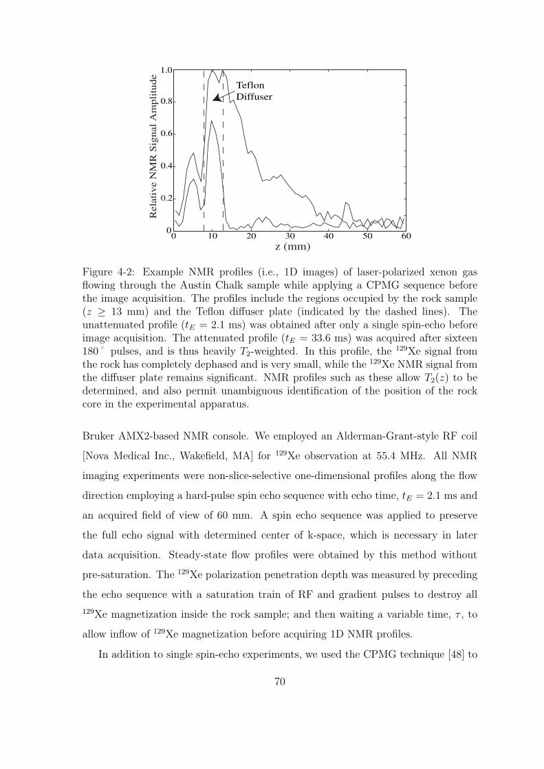
0 10 20 30 40 50 600
0.2
0.4
0.6
0.8
1.0
Teflon
Diffuser
Rela
tiv
e N
MR
Sig
nal
Am
pli
tud
e
z (mm)
Figure 4-2: Example NMR profiles (i.e., 1D images) of laser-polarized xenon gasflowing through the Austin Chalk sample while applying a CPMG sequence beforethe image acquisition. The profiles include the regions occupied by the rock sample(z ≥ 13 mm) and the Teflon diffuser plate (indicated by the dashed lines). Theunattenuated profile (tE = 2.1 ms) was obtained after only a single spin-echo beforeimage acquisition. The attenuated profile (tE = 33.6 ms) was acquired after sixteen180˚ pulses, and is thus heavily T2-weighted. In this profile, the 129Xe signal fromthe rock has completely dephased and is very small, while the 129Xe NMR signal fromthe diffuser plate remains significant. NMR profiles such as these allow T2(z) to bedetermined, and also permit unambiguous identification of the position of the rockcore in the experimental apparatus.
Bruker AMX2-based NMR console. We employed an Alderman-Grant-style RF coil
[Nova Medical Inc., Wakefield, MA] for 129Xe observation at 55.4 MHz. All NMR
imaging experiments were non-slice-selective one-dimensional profiles along the flow
direction employing a hard-pulse spin echo sequence with echo time, tE = 2.1 ms and
an acquired field of view of 60 mm. A spin echo sequence was applied to preserve
the full echo signal with determined center of k-space, which is necessary in later
data acquisition. Steady-state flow profiles were obtained by this method without
pre-saturation. The 129Xe polarization penetration depth was measured by preceding
the echo sequence with a saturation train of RF and gradient pulses to destroy all
129Xe magnetization inside the rock sample; and then waiting a variable time, τ , to
allow inflow of 129Xe magnetization before acquiring 1D NMR profiles.
In addition to single spin-echo experiments, we used the CPMG technique [48] to
70

measure the 129Xe spin coherence relaxation time (T2) in the rock sample and diffuser
plate, with tE = 2.1 ms and one to sixteen 180˚ RF pulses prior to echo acquisition.
For each point in the profile, we fit the amplitude decay, as a function of the number
of echo loops before acquisition, to an exponential to yield T2(z). Fig. 4-2 shows
example T2 weighted profiles from such an acquisition sequence. After sixteen 180◦
pulses (33.6 ms), the xenon magnetization in the rock has completely dephased, but
is clearly visible in the inflow tube and diffuser, thereby allowing us to define the start
of the rock with an accuracy of about 1 mm (equivalent to the spatial resolution of
the 1D NMR images).
To confirm the NMR experiments, three of the five rock samples (Fontainebleau
sandstone, Austin chalk and Edwards limestone) were also characterized indepen-
dently using standard techniques by a commercial company [New England Research,
White River Junction, VT]. This company used a gas pycnometer to determine ab-
solute porosity from gas pressure changes via Boyle’s Law [49]. They measured per-
meability via the steady-state gas flow method with a standard gas permeameter
[37, 38]. In these standard measurements, the accuracy of the absolute porosity value
is generally accepted to be ∼ 1%, and that of the permeability value ∼ 10 – 20%.
4.3 Effective Porosity Measurement and Results
To determine the effective porosity, we measured 129Xe NMR spin echo profiles from
each sample under the condition of steady-state polarized gas flow. Fig. 4-3 shows
profiles acquired for all the rock samples. The amplitude of the profile at each point
along the sample is proportional to the 129Xe gas density and spin polarization, the
void space volume participating in gas flow, and the effect of spin coherence relax-
ation. As discussed in the next section, we corrected for gas density and polarization
variation along the rock (see Fig. 4-3), such that the ratio of profile amplitudes in
the diffuser plate (a medium of known porosity) and the rock was proportional to
the ratio of the average void space volumes contributing to fluid flow in the two re-
gions, with weighting factors accounting for T2 relaxation. Our measurements of T2
71

0 10 20 30 40 50 600.0
0.2
0.4
0.6
0.8
1.0
FontaineBleau
Effective porosity
= (11.3 ± 0.7)%Teflon
Diffuser
Rela
tiv
e N
MR
Sig
nal
Am
pli
tude
z (mm)0 10 20 30 40 50 60
0.0
0.2
0.4
0.6
0.8
1.0
Austin chalk
Effective porosity
= (18.4 ± 0.9)%
z (mm)
Rela
tiv
e N
MR
Sig
nal
Am
pli
tude
a) b)
0 10 20 30 40 50 600.0
0.2
0.4
0.6
0.8
1.0
z (mm)
Rela
tiv
e N
MR
Sig
nal
Am
pli
tude
Edwards limestone
Effective porosity
= (15.1 ± 1.1)%
c)
0 10 20 30 40 50 600.0
0.2
0.4
0.6
0.8
1.0
z (mm)
Bentheimer
Effective porosity
= (11.2 ± 1.2)%
d)
Rela
tiv
e N
MR
Sig
nal
Am
pli
tude
0 10 20 30 40 50 60
Indiana limestone
Effective porosity
= (7.10 ± 0.6)%
e)
0.0
0.2
0.4
0.6
0.8
1.0
Rela
tiv
e N
MR
Sig
nal
Am
pli
tud
e
z (mm)
Figure 4-3: NMR profiles (i.e., 1D images) of laser-polarized xenon gas flowingthrough samples of (a) Fontainebleau sandstone, (b) Austin Chalk, (c) Edwardslimestone, (d) Bentheimer and (e) Indiana limestone, with both the gas flow rateand xenon magnetization in steady state. The profiles include the regions occupiedby the rock sample and the Teflon diffuser plate (indicated by dashed lines). Thebold lines show the profiles corrected for gas density and polarization variation in therock. For such typical NMR profiles, we averaged 32 signal acquisitions, each madewith tE = 2.1 ms, and achieved a 1D spatial resolution of approximately 1 mm.
72

as a function of position along the sample yielded distinct values corresponding to
129Xe in the diffuser plate (T dif2 = 76.8 ms) and the rock cores (T rock
2 = 4.59 ms in
Fontainebleau sandstone and 12.3 ms in Austin Chalk). (These differences in T2 arise
from differences in magnetic susceptibility and hence background magnetic gradients,
as well as differing wall interactions.)
Hence, we determined the effective porosity of the sample from the relation:
φe =Adif
Arock
Srock
Sdif
exp(−tE/T dif2 )
exp(−tE/T rock2 )
, (4.3)
where Adif is the cross-sectional area of void space in the diffuser; Arock is the rock
sample cross-sectional area; Sdif and Srock are the NMR profile amplitudes in the
diffuser and the rock respectively; and tE is the echo time used to acquire the profile.
129Xe spins located in isolated or dead-end pores larger than the one-dimensional gas
diffusion length during tE (∼ 50 µm for our experimental conditions) contributed
no significant NMR signal to the effective porosity measurement. We determined the
rock profile amplitude (Srock) at a distance of 1 mm from the diffuser-rock interface on
the upstream side of the gas flow. This 1 mm offset was chosen so that no 129Xe in the
diffuser contributed to Srock, and so that insignificant depolarization had occurred for
the 129Xe in the well-connected pores that contribute to the rock’s effective porosity
and permeability. We also used the 1 mm offset point in the rock profile to calculate
the correction for gas density and polarization variation along the rock. For additional
1 mm offsets, we found that the effective porosity derived from our measurements
varied by less than other sources of uncertainty: the fractional variations for all the
rock samples are less than 7%. Table 4.1 lists the effective porosities we determined
for the Fontainebleau sandstone, Austin Chalk and Edwards limestone, as well as
the absolute porosities determined using the gas pycnometer. Results on the two
other rock cores are also included, but without comparison measurements using the
standard method.
73

4.4 Permeability Measurement and Results
The permeability of a porous medium is generally determined from the volume flow
rate of fluid under a given pressure gradient [38]. Here, we employed NMR imaging
to determine the flow rate of laser-polarized 129Xe gas through reservoir rocks, using
the pre-saturation method described above to image only xenon spins that flow into
the rock during a defined period.
A one-dimensional NMR profile acquired with a spin-echo sequence provides a
good representation of the spatial distribution of spin magnetization per unit length,
M(z), which can be expressed as [18]:
M(z) = A · φe · n(z) · λ · p(z) · (γ~I), (4.4)
where A is the cross-sectional area of the sample; φe is the effective porosity; n(z) is
the gas number density along the direction z of gas flow; λ is the isotopic abundance
of 129Xe nuclear species in the Xe gas; p(z) is the 129Xe spin polarization; and γ~I is
the spin magnetization per polarized 129Xe atom (nuclear spin I = 1/2). On length
scales > 1 mm, where φe is spatially uniform for the rocks we studied, only the
number density, n,and polarization, p, are spatially dependent. The parameters, n
and p, as well as the gas velocity, v, and spin relaxation time, T1, fluctuate greatly
within the pore length-scale, due to the complicated pore structure in reservoir rocks.
Our experiment was only sensitive to cross-sectional averages of these parameters,
resulting in a z-dependent measurement on a scale ∼ two orders larger than the
typical pore size.
Assuming uniform laminar flow (a reasonable assumption for the very low Reynolds
number, Re ∼ 10−5, of these experiments), the 1D distribution of the gas number
density inside the rock sample is given by [50]:
n(z) =1
kBT
√P 2
i − (P 2i − P 2
o )z
L, (4.5)
where Pi and Po are the inlet and outlet gas pressures across the sample; L is the
74

sample length; kB is Boltzmann’s constant; and T is the gas temperature.
The relaxation of xenon spins in the rock is dominated by surface interactions
with paramagnetic impurities at the grain surfaces. Bulk xenon spin relaxation due
to xenon-xenon collisions is several orders of magnitude slower [34]. Therefore, T1
for xenon infused in a porous rock can be well-approximated as a mono-exponential
decay of magnetization. The 129Xe spin polarization decreases along the flow path
due to spin relaxation in the rock; the attenuation over a spatial displacement dz
being dp(z)dz
= −1v(z)T1(z)
, where v(z) is the spatially-dependent gas flow velocity and
T1(z) is the spatially-dependent mono-exponential relaxation time. While a single Xe
atom travels along random tortuous paths defined by the microscopic pore structure,
v(z) represents the statistically averaged spin displacement, averaged over all spins in
a plane perpendicular to the flow direction. Applying Darcy’s Law, for v(z) = ~qAφe
,
having the gas number density inside the rock (Eq. (4.5)) in mind and assuming that
129Xe gas follows the ideal gas law, one finds:
v(z) = − k
φeµ
dP
dz=
1
2
k
φeµ
P 2i − P 2
o
LP (z). (4.6)
where the spatially-dependent xenon gas pressure, P (z) = n(z)kBT , µ is the xenon
viscosity and k is the sample permeability. The spatial dependence of polarization is
therefore found to be:
p(z) = p0 exp(−z∫
0
dz
v(z)T1(z)) = p0 exp(−2φeµ
kβ
L
P 2i − P 2
o
z) , (4.7)
where p0 = p(z = 0) and β relates the 129Xe T1 to gas pressure via T1(z) = β P (z),
assuming T1 is dominated by wall relaxation and hence by gas diffusion to pore walls
[51], a reasonable assumption given the long inherent bulk 129Xe T1.
Combining Eqs. (4.4) to (4.7), the spatial dependence of the 129Xe spin magneti-
zation per unit length in a porous rock can be written as
75

M(z) = Aφeλ1
kBT(γ~I) p0
√P 2
i − (P 2i − P 2
o )z
Lexp(−2φeµ
kβ
L
P 2i − P 2
o
z) . (4.8)
Our permeability experiments were performed with a steady state gas flow, but
with a zero initial 129Xe spin polarization, created by the application of a series of fast
RF and magnetic field gradient pulses to spoil any spin polarization in the sample
on timescales of 20 ms, which is much faster than the time for gas transport through
the sample (on the order of 10 s). During a subsequent delay or propagation time,
τ , polarized gas entered the sample, after which we acquired an NMR profile. We
repeated this process for different propagation times, thereby revealing the rate of
flow of laser-polarized 129Xe gas through the rock’s pore space. Data for all the rock
cores are shown in Fig. 4-4. The penetration depth, ξ, was calculated at each τ by
dividing the total 129Xe NMR signal in the rock, determined from the MRI profile
integrated over the rock length, by the signal amplitude at z = 0. We measured the
inlet and outlet pressures Pi and Po with bridge pressure sensors. (For example, Pi ≈3.73 bar and Po ≈ 0.78 bar for the low-permeability Austin Chalk, and Pi ≈ Po ≈4.33 bar for the high permeability Fontainebleau.) Also, we used the xenon viscosity
µ = 2.324 × 10⁻⁵ Kg/m-s, for the typical experimental temperature of 25˚C [52].
(Gas viscosity is essentially independent of pressure and only minimally temperature
dependent [52].) Using Eqs. (4.5) and (4.6) as well as the ideal gas law (P (z) =
n(z)kBT ), we derived a relation between the propagation time τ and penetration
depth ξ:
τ =
ξ∫
0
dz
v(z)=
4
3
φeµ
k
L2
(P 2i − P 2
o )2
{P 3
i −[P 2
i − (P 2i − P 2
o )ξ
L
] 32
}. (4.9)
From Eq. (4.9), we determined each rock’s permeability, k, using the experimen-
tally measured values for Pi, Po and L, the known value of µ, and the values of ξ
calculated from the NMR profiles.
76

15 20 25 30 35 40 45 500.0
0.2
0.4
0.6
0.8
1.0
Fontainebleau
Permeability
k = 559 ± 93 mD
Rela
tiv
e N
MR
Sig
nal
Am
pli
tude
τ = 1.0 s 1.5 s 2.0 s
z (mm)10 15 20 25 30 35 40 45
0.0
0.2
0.4
0.6
0.8
1.0
τ = 2 s
Rela
tiv
e N
MR
Sig
nal
Am
pli
tud
e
z (mm)
Austin chalk
Permeability
k = 2.6 ± 0.3 mD
4 s 6 s
10 15 20 25 30 35 40 450.0
0.2
0.4
0.6
0.8
1.0
τ = 2.0 s 3.0 s 4.0 s
Edwards limestone
Permeability
k = 7.0 ± 0.9 mD
z (mm)
Rela
tiv
e N
MR
Sig
nal
Am
pli
tude
15 20 25 30 35 40 450.0
0.2
0.4
0.6
0.8
1.0
z (mm)
τ = 1 s 2 s 3 s
Bentheimer
Permeability
k = 123 ± 24 mD R
ela
tiv
e N
MR
Sig
nal
Am
pli
tude
20 22 24 26 28 30 320.0
0.2
0.4
0.6
0.8
1.0
Rela
tiv
e N
MR
Sig
nal
Am
pli
tud
e
z (mm)
Indiana sandstone
Permeability
k = 0.18 ± 0.03 mD
τ = 8 s 11 s
14 s
Figure 4-4: 129Xe NMR profiles used in the permeability measurements: (a)Fontainebleau sandstone, (b) Austin Chalk, (c) Edwards limestone, (d) Bentheimerand (e) Indiana limestone. Profiles shown in solid lines correspond to different delaytimes, τ , following a sequence of RF and gradient pulses to quench all xenon mag-netization in the sample. The dash lines are profiles corrected for gas density andpolarization variation.
77

For both the effective porosity and permeability measurements, we corrected for
gas density and spin polarization variations as described in the following. We fit the
129Xe NMR profiles from each rock sample, measured with steady-state xenon flow
and without prior polarization destruction (e.g., the profiles shown in Fig. 4-3), to
Eq. (4.8). From these fits we determined the exponential decay rate, 2φeµkβ
LP 2
i −P 2o.
Then, we removed the pressure and spin-relaxation dependence of each profile by
dividing Srock (determined at a 1 mm offset from the diffuser-rock interface) by
1Pi
√P 2
i − (P 2i − P 2
o ) zL
exp(−2φeµkβ
LP 2
i −P 2oz), which is normalized to unity at 1 mm from
the entrance of the rock sample. After this correction (see Figs. 3 and 4), profile
amplitudes depended only on the fractional volume of the rock occupied by flow-
ing laser-polarized xenon. Table 4.1 lists the permeabilities we determined for the
Fontainebleau sandstone, Austin Chalk and Edwards limestone, as well as the per-
meabilities obtained independently using the gas permeameter. We also include mea-
surement results on the two other rock cores, without comparison measurements with
the standard method.
Table 4.1: Permeability and Effective Porosity ResultsSample Permeability (mD) Effective
Porosity (%)AbsolutePorosity (%)
LP-XenonMRI
GasPermeameter
LP-XenonMRI
GasPycnometer
Fontainebleau 559 ± 93 589 ± 117 11.3 ± 0.7 12.5 ± 0.6Austin Chalk 2.6 ± 0.3 3.6 ± 0.7 18.4 ± 0.9 29.7 ± 1.5Edwards limestone 7.0 ± 0.9 4.76 ± 0.95 15.1 ± 1.1 23.3 ± 1.2
Bentheimer 123 ± 24 NA 11.2 ± 1.2 NAIndiana limestone 0.18 ± 0.03 NA 7.10 ± 0.60 NA
After determining the effective porosity and permeability of each sample, we de-
termined the spin relaxation rate proportionality coefficient, β from the exponential
decay rate derived from fitting 129Xe NMR profiles to Eq. (4.8). For the Fontainebleau
sample, the 129Xe spin relaxation time (T1) could therefore be calculated from the
nearly constant gas pressure in the sample (Pi ≈ Po ≈ 4.33 bar), yielding T1 = 6.0
± 1.0 s. To test the validity of Eq. (4.8) and the method of profile correction, we
measured the 129Xe T1 directly; we created a sealed container holding a large sample
78

of Fontainebleau sandstone and thermally-polarized 129Xe at the same gas pressure
used in the flowing, laser-polarized gas experiment. The result of 5.6 ± 0.3 s agrees
well with the T1 value derived from the flowing, laser-polarized gas experiment.
As shown in Table 4.1, the permeability values measured with the NMR method
are in reasonable agreement with those measured with gas permeameter taking into
account the one-standard-deviation uncertainties in these numbers. We therefore
conclude that the NMR method provides an accurate measure of permeability.
4.5 Error Analysis
We estimated uncertainties in the NMR measurements of effective porosity and per-
meability by error propagation of known uncertainties in the directly measurable
quantities: NMR signal amplitudes and integrations, gas pressure, dimensions of the
samples and diffuser, as well as experimental timings. The uncertainties in rock sam-
ple dimensions and NMR experimental timing are on the order of 0.5%, which is
negligible compared to that due to the other factors. Here we only consider propaga-
tion of errors arising from noise in the NMR signals and uncertainties in the pressure
measurements. Next we show as an example the procedure to estimate the uncer-
tainty in the effective porosity.
Eqn. (4.3) describes the calculation of effective porosity value from the cross-
sectional area, A, profile signal intensity, S and T2 in the rock and diffuser, respec-
tively. By ignoring errors in measuring A and tE, we have the following equation for
evaluating error in the effective porosity:
∆φ
φ=
∆Srock
Srock
+∆Sdif
Sdif
+tE∆T rock
2
(T rock2 )2
+tE∆T dif
2
(T dif2 )2
, (4.10)
according to the rule of error propagation [53]. To calculate ∆S, we find n consecutive
data points representing pure noise in the profile where no 129Xe signal was present,
and ∆S is equal to the standard deviation in the intensity values of the n points. In
the same profile, ∆Srock = ∆Sdif . We determine T rock2 by first integrating the portion
of the profile corresponding to the rock sample, and then fitting the integral Irock to
79

an exponential. Suppose the length of the rock sample is N , measured in the number
of data points in the profile. We then have
∆Irock =√
N∆Srock, (4.11)
for the uncertainty in the integrals since the noise-induced fluctuations are not sta-
tistically correlated. I is related to time t by the exponential function I = Ce−t/T2 ,
and T2 is available by least-squares fitting to the following linear relation,
lnI
C= − t
T2
, (4.12)
and the uncertainty in the fitting result is given by (see Appendix E or [53])
∆T2 = T 22
√√√√ 1
∆
n∑i=1
1
σ2i
, (4.13)
where σi and ∆ are
σi =∆Ii
Ii
, (4.14)
∆ =n∑
i=1
1
σ2i
n∑i=1
t2iσ2
i
−( n∑
i=1
tiσ2
i
)2
,
in which Ii are integrals of the profiles measured at time ti.
Uncertainty in the permeability k is obtained by first estimating errors in the
penetration depth, ξ, and the pressure values2, and then arranging Eqn. (4.9) into
a linear relationship between τ and ξ, from which uncertainty in k can be deter-
mined through a similar linear-fitting technique to that shown above for the effective
porosity.
2According to the specifications for the pressure sensor, the uncertainty in measured pressure is0.5 psi.
80

4.6 Discussions and Conclusions
The laser-polarized noble gas NMR measurement of permeability agrees well with
measurements made using the standard gas permeameter technique, for the represen-
tative high and low permeability rocks studied so far. For values above 500 mD and
below 5 mD, the NMR method yields permeability results that are well within the
uncertainty range of the values measured using the gas permeameter, and shows that
large variations in the parameters used to determine k, (e.g., output pressure, Po), do
not detract from the measurement. In addition, the effective porosity simultaneously
measured by the NMR technique shows that as permeability decreases, the effective
porosity measured is a decreasing fraction of the absolute porosity determined by
the standard gas pycnometer technique. Effective porosity (i.e., the volume fraction
of pore spaces that contribute to fluid flow through the material) is always smaller
than the absolute porosity of a sample, and is a parameter that is not easily, nor
directly determined with other techniques. The Fontainebleau sandstone has a high
permeability due to its well-connected pores with a narrow distribution of sizes, a
fact that is consistent with the finding that the sample core has an effective poros-
ity nearly as large as its absolute porosity. Conversely, Austin Chalk and Edwards
limestone exhibit effective porosity values that are almost half the values of their
absolute porosity, consistent with the knowledge of its very low permeability due to
poor pore interconnectivity. The case of Bentheimer sandstone is similar to that of
Fontainebleau, where a relatively smaller pore volume, but good pore interconnec-
tions are found. The results in Indiana limestone show both low effective porosity
and permeability, which could be attributed to a higher resistance to flow due to the
narrowed pathways, as well as possible poor inter-pore connections.
To perform NMR imaging of the penetrating inflow of laser-polarized xenon gas,
the 129Xe spin decoherence time (T2) in the rock samples must be sufficiently long (∼2 - 5 ms), for a spin echo profile to be obtained without significant signal loss. For
the Fontainebleau and Austin Chalk samples, both relatively free of paramagnetic
impurities, this condition is easily satisfied, with the measured 129Xe T2 at 4.7 T
81

being 4.59 and 12.3 ms in the pores of the Fontainebleau and Austin Chalk, respec-
tively. However, the paramagnetic impurities in many rocks, especially sandstones,
will produce large magnetic field gradients when placed in magnetic fields ≥ 1 T, these
background gradients will significantly shorten the 129Xe T2. One such example was
Berea 100, a macroscopically homogeneous, high-permeability [39] sandstone with a
narrow distribution of pore diameters of ∼ 100 µm, but with a significant content
of paramagnetic particles. In this sample, we were unable to measure a spin echo
profile at 4.7 T from inflowing laser-polarized xenon, and hence could not measure
the effective porosity or permeability. For such samples, it should be practical to
operate at applied magnetic fields << 1 T for two reasons; (i) the magnetization
of laser-polarized noble gas is determined by the optical pumping process external
to the applied NMR magnetic field, B0, i.e., the laser-polarization obtained is inde-
pendent of B0, whereas for thermally-polarized samples it is proportional to B0; and
(ii) the magnetic field gradients induced in porous media by magnetic susceptibility
variations scale with B0 and hence are greatly reduced for small B0. We have previ-
ously demonstrated that NMR images of laser polarized noble gas can be acquired at
applied field strengths as low as 20 G with resolution and SNR comparable to NMR
images obtained at magnetic field strengths ∼ 1 T [20, 54]. Low-field NMR of flowing
laser-polarized noble gas may allow effective porosity and permeability measurements
in a wide array of porous samples using a simple, low-cost electromagnet. In addition
to reservoir rocks, this technique may be applicable to ceramics, fluidized beds, filters
and partially liquid-saturated porous media [55, 56].
In conclusion, we have demonstrated the simultaneous measurement of permeabil-
ity and effective porosity of high and low permeability oil-reservoir rock cores using
NMR imaging of the penetrating flow of laser-polarized xenon gas. The method is
accurate, with permeability results that cover a range of more than two orders of
magnitude and agree well with the results from standard techniques. The method is
also fast and reproducible: the procedure typically requires about 15 minutes, which
is considerably less time-consuming than other NMR-based methods [50] and some
standard techniques [41, 42]. The effective porosity measurements are consistent with
82

expectations: the effective porosity is found to be nearly as large as the absolute poros-
ity for the high permeability Fontainebleau sandstone, and to be significantly smaller
than the absolute porosity for lower permeability samples such as Austin Chalk and
Edwards limestone.
83

84
Chapter 5
Introduction to Gas-Fluidization
5.1 Background
Granular media are collections of small solid particles which are ubiquitous in the food
processing industry and nature. These particles are solids, but under certain condi-
tions a collection of them will tend to behave like a liquid. Some examples of granular
materials include food products (rice, corn and salt), building materials (sand, gravel
and soil) and chemicals (aluminum powder, plastic and pharmaceuticals). Statistics
show that in the chemical industry, approximately one half of products and one third
of raw materials are granular media [57]. Moreover, it is estimated that tens of billions
of dollars are being spent in the industry of particle technology [58]. Diagnosing the
dynamics of these materials is relevant to a wide range of scientific and technological
problems. Granular chemicals are processed in various kinds of chemical reactors, and
the design and performance of these reactors rely significantly on the understanding
of the behaviors of the materials under different operating conditions.
Gas fluidization is a process in which solid particles experience fluid-like suspen-
sion in a stream of upflowing gas. Five different fluidization may be observed, listed
in the order of increasing gas flow rate: fixed bed, homogeneous fluidization, bub-
bling fluidization, slugging and pneumatic transport [1]. Fig. 5-1 shows the regimes
schematically. A fixed bed represents static packed particles, through which gas flows
without changing the solid configuration. Homogeneous fluidization is the start of
85

Figure 5-1: Five different fluidization regimes: fixed bed, homogeneous fluidization,bubbling fluidization, slugging and pneumatic transport. Originally found in [1].
particle suspension, initiated when the weight of the particles is balanced by drag
forces from the gas, which include viscous drag, inertial drag and buoyancy. Bubbles,
or void spaces with volumes much larger than that of single particles, emerge when
the gas flow rate is further increased. Two phases exist in a bubbling bed: one is a
bubble phase with almost no particles inside, and the other is the remaining solid-gas
mixture with a high particle number density, and which is called the emulsion phase.
The fast rising bubbles enhance circulation and mixing of particles throughout the
bed, in which concentration and temperature gradients can be quickly relaxed. This
is the reason why the bubbling regime has been widely applied. Slugging is the term
for the regime in which the diameter of the bubbles approaches that of the container,
especially for fast flows through a deep particle bed. Pneumatic transport occurs
when the flow rate is so high that it continuously pushes the particles along with the
gas and out of the bed.
Despite the wide application of fluidization, the understanding of the dynamics of
both the solid particles and the gas is far from complete, as such a system is difficult
to model numerically, primarily due to the large number of degrees of freedom and
inelastic collisions among the particles [2]. Filled up by solid particles, a typical three-
86

dimensional fluidized granular system is opaque, resulting in difficulties using light
scattering or sound waves to experimentally probe the bed behavior deep under its
surface [59].
Recently, considerable interest has arisen in studying the behaviors of solid parti-
cles in gas-fluidized beds. The question about whether the homogeneously fluidized
particles are fluid-like, i.e., they are completely suspended by drag forces from the flu-
idizing gas or whether they behave like a soft solid in which interparticle stresses exist,
has been a matter of debate. Rietema [60] discussed the different types of coherent
forces between the solid particles and their effects on the homogeneous bed expan-
sion. Tsinontides and Jackson [61] experimentally determined that the stabilization
of homogeneous fluidization was achieved by the presence of yield stresses among the
particles. Menon and Durian [62] measured the particle velocity fluctuations by using
diffusion-wave spectroscopy (DWS), and observed no particle motions in the homoge-
neous fluidization regime. They hence concluded that, in this regime, the ensemble of
particles was more like a solid, supported by enduring contacts. Valverde et al. [63]
studied the concentration of fine toner particles (∼ 8.53 µm) under different gas flow
conditions, and found that the bed was more solid-like when the gas flow velocity was
below a given threshold, while fluid-like behavior such as particle diffusion was ob-
served when the gas flow was above the threshold. However, Foscolo and Gibilaro [64]
proposed that the interaction between the particles and the fluidizing gas resulted in
the fluid-like suspension of the particles, and they studied the stability of the suspen-
sion, as well as its transition into the unstable bubbling regime. In summary, there
is no consensus regarding particle motion in the homogeneous fluidization regime,
and more experimental evidence, especially with different measurement approaches
and different particle sizes and densities, is needed to better understand of the phe-
nomenon. Previous experimental works have investigated the mechanics of the solid
particles, but no studies have been conducted to investigate the flow characteristics
of the fluidizing gas - which is another crucial factor in the process.
Most commercial fluidized beds operate in the bubbling fluidization regime, in
which bubbles emerge at the bottom and expand while rising up along the bed.
87

Bubbles help to agitate the bed to achieve better mixing, but they also provide a
shortcut route for gas to escape the bed without coming in contact with the solid
particles [65]. For gas molecules in bubbles to react with the solid phase, they must
undergo two processes: transitioning to the emulsion (or interstitial space) from the
bubbles, and then migrating to the solid phase, where they are adsorbed. The gas
exchange rate is a measure of the efficiency of the contact between the solid and
gas phases, and has a significant effect on the operation of the fluidized bed. For
example, the reaction rate and yield for a given amount of gas in most chemical
reactors is limited by the gas exchange rate; the efficiency of removing moisture in a
drying process is also related to the exchange rate. Our aim in this research was to
develop a new methodology for measuring gas exchange non-invasively, based on the
technologies of NMR and laser-polarization of noble gas.
5.2 Introduction to Fluidized Bed Operations
5.2.1 Components of a Fluidized Bed
A fluidized bed is functionally comprised of four components: the column, gas dis-
tributor, particles, and gas flow.
The column is a container that keeps the gas and particles inside its walls and is
vertically orientated with openings at both its top and bottom. In industrial practice,
the inner surface of the column experiences harsh conditions, and as such it may be
either attrited by frequent particle collisions or corroded by reactive species in the
bed [1]. In research, the column is often chosen to be transparent so that the bed
surface dynamics are easily observed from outside.
A gas distributor is a material with interconnected pores through which the gas
flows. Distributors support the particles, and keep the entering gas flow homogeneous
in cross-section; they therefore need to be made from a stiff porous material. The
criterion for choosing a proper distributor is to make the minimum pore size smaller
than the diameter of the smallest particles to prevent the particles from leaking
88
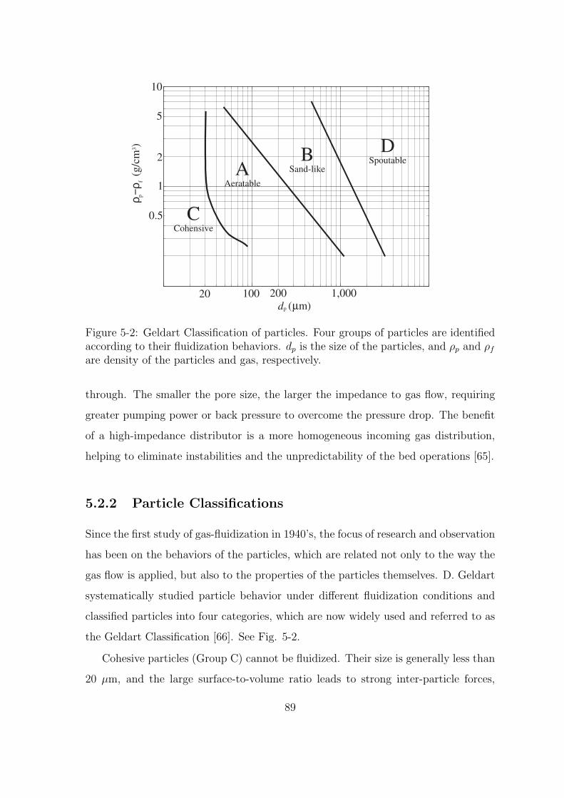
ρ −ρ
(
g/c
m )
fp
3
dp (µm)20 100 200 1,000
0.5
1
2
5
10
CCohensive
AAeratable
BSand-like
DSpoutable
Figure 5-2: Geldart Classification of particles. Four groups of particles are identifiedaccording to their fluidization behaviors. dp is the size of the particles, and ρp and ρf
are density of the particles and gas, respectively.
through. The smaller the pore size, the larger the impedance to gas flow, requiring
greater pumping power or back pressure to overcome the pressure drop. The benefit
of a high-impedance distributor is a more homogeneous incoming gas distribution,
helping to eliminate instabilities and the unpredictability of the bed operations [65].
5.2.2 Particle Classifications
Since the first study of gas-fluidization in 1940’s, the focus of research and observation
has been on the behaviors of the particles, which are related not only to the way the
gas flow is applied, but also to the properties of the particles themselves. D. Geldart
systematically studied particle behavior under different fluidization conditions and
classified particles into four categories, which are now widely used and referred to as
the Geldart Classification [66]. See Fig. 5-2.
Cohesive particles (Group C) cannot be fluidized. Their size is generally less than
20 µm, and the large surface-to-volume ratio leads to strong inter-particle forces,
89

which originate from various sources such as electrostatic charge, moisture, sticky
particle surfaces, soft solid and irregular particle shapes. As a result, the particles
move cohesively as the gas flow is aupplied, and the agglomeration of particles is
difficult to break. Under certain situations, manual stirring is helpful in slightly
fluidizing this category of particles. However, Group C particles are usually not
chosen for fluidization.
Areatable particles (Group A) are easily fluidized. They correspond to a rela-
tively small particle size and low density. Homogeneous expansion of the bed is only
observed in this category of particles, and considerable bed expansion can occur. In-
terparticle forces are still large but drag forces from the gas are capable of breaking
the particle cohesion. Different fluidization regimes are available and conveniently
controlled by adjusting gas flow rate. Most light powders sized below 80 µm belong
to this group.
Sand-like particles (Group B), with size between 40 and 500 µm and density
between 1.4 and 4 g/cm3 are widely used for fluidization. The interparticle forces are
negligible compared to the larger weight of each particle and stronger interactions with
the fluidizing gas. Homogeneous fluidization is not observed with bubbles emerging
immediately when the bed is fluidized.
Spoutable particles (Group D) are large and dense, and hence difficult to fluidize.
When gas flow is supplied, thin channels appear in the bed, allowing the flow through
the particle bed. In the case of strong channelling, erratic particle behavior such as
spouting may occur.
Geldart made the phenomenological classification by simply generalizing the bed
behavior associated with differences in density and size of the particles. This classi-
fication is extremely helpful in choosing the correct type of particles for specific flu-
idization regimes. However, there is no rigorous theoretical work that quantitatively
explains this empirical classification, because of the the complexity of modelling the
particle motions and inter-particle forces in such a system.
90

5.2.3 Homogeneous and Bubbling Fluidization
In this section, the onset of fluidization and particle/gas flow behavior in the two
regimes will be covered.
Homogeneous Fluidization
Suppose we have a bed of randomly packed particles belonging to Geldart Group A.
Without gas flow, the fixed bed demonstrates no particle motions. If we start to flow
gas through at a very slow rate, the particles will not fluidize, but behave like a porous
material through which flowing gas flow passes through the interstitial spaces. When
the Reynolds number (Re = ρgUd
µ) is far less than unity, viscous drag dominates and
the relationship between the gas pressure drop, ∆P , and the average flow velocity is
linear according to Darcy’s law [37]. From the Carman-Kozeny equation [67], which
is an extended Darcy equation onto flow through a pack of spherical beads, we have
∆P
H=
150(1− ε)2
ε3
µU
d2, (5.1)
where H is the bed height; ε is void fraction, or ratio of interstitial volume to total
bed volume (i.e., porosity), which varies between 0.4 and 0.7 with a weak dependence
on the size, shape and density of particles; µ is the gas viscosity; U is the superficial
or empty tube velocity, the velocity at which the gas would flow in the column if all
of the particles were removed while the input flow of gas was kept constant; and d is
average particle diameter. 1
As the gas flow rate increases, the pressure drop ∆P in Eqn (5.1) increases linearly
until it equals the total weight of particles divided by the bed cross-sectional area,
which is the threshold for incipient fluidization, also called minimum fluidization.
This condition can be written as
1For particles with non-spherical shape, the diameter refers to that of a sphere with the samesurface-to-volume ratio as the particles. If mixed-size particles are used, the average diameter iscalculated by 1/(
∑i xi/di), in which di is the diameter and xi the weight fraction of particles with
such a diameter [65]
91

ρp(1− εmf )g =150(1− εmf )
2
ε3mf
µU
d2, (5.2)
where ρp is particle density; g is gravitational acceleration; and εmf is the void fraction
of the bed corresponding to minimum fluidization. The left hand side of represents
the weight of the particles divided by total bed volume. The superficial velocity Umf
for minimum fluidization is hence
Umf =ε3mfρpgd2
150(1− εmf )µ, (5.3)
which is useful for estimating the flow velocity needed to start fluidization of spherical
particles. In the case of fine powders, Wen and Yu recommended using [68]
Umf =µ
dρg
[33.72 + 0.0408
d3ρg(ρp − ρg)g
µ2
]1/2
−33.7, (5.4)
where ρg is gas density. This empirical relationship is particularly useful when the
particle shape is irregular and void fraction of bed is unknown, but it does not apply
to spherical particles.
Homogeneous fluidization starts once the gas velocity is larger than Umf , or when
the weight of the particles is completely balanced by the drag forces. If the gas flow
velocity increases further, the drag forces will no longer change but be constant and
equal to the particle weight. Instead, the particles re-configure, so that the bed of
particles does not move. As a result, the interstitial space expands and εmf in Eqn.
(5.2) will increase so that the equation still holds.
In homogeneous fluidization, the movement of particles is minimal and such a
collection of fluidized particles has been referred to as “weak solid” [62], where en-
during inter-particle contacts exist even though the majority of the particle weight
is balanced by the gas. The true fluid-like behavior starts only after bubbles are
generated.
92

Bubbling Fluidization
The emergence of bubbles usually starts as a bumpy top surface of the bed, once the
flow velocity goes higher than a threshold known as the minimum bubbling velocity,
Umb, compared to Umf . It is considerably more difficult to predict Umb, and only
empirical relations are available to estimate the value. Geldart and Abrahamsen
discovered that Umb is highly dependent on the fraction of particles sized under 45
µm [69].
The shape of a bubble is close to a sphere, except for a concave bottom generated
when rising bubbles leave a trailing low-pressure void that is quickly filled by nearby
particles. Fig. 5-3 shows a photo of a bubble in a two-dimensional fluidized bed,
together with gas flow streamlines calculated from Davidson’s bubble model. Note
the gas circulation at the two sides, which is caused by the fact that the bubble always
rises at a much faster velocity in our experimental conditions (typically 10 times
faster) than the gas flow in the emulsion. The volume occupied by the circulating gas
is often referred to as a “cloud”, in which gas flow is largely impeded by particles.
The cloud surrounding the bubble forms a layer between the bubble and the emulsion,
which is expected to impede the gas exchange in and out of the bubbles. A cloud
layer exists only when the bubble velocity ub is larger than the gas flow velocity uf
in the emulsion phase. If ub < uf , no gas cloud will form. In our experiments with
fine powders, the flow velocity in the emulsion phase is ∼ 1 cm/s while the velocity of
any observable bubble (with a diameter larger than the particle size) is above 2 cm/s,
resulting in the presence of a cloud layer around any bubble. The ratio of cloud to
bubble volume is given by [1]
fc =2uf
ub − uf
. (5.5)
The calculated cloud volume is 50% of the bubble volume when the bubble size
is 0.5 mm, but decreases to 20% as the bubble size increases to 2 mm. For bubbles
with a diameter > 0.1 mm, the cloud is much less than the bubble diameter.
The motion of bubbles agitates the otherwise quasi-static homogeneous fluidiza-
93

a b
Cloud
Figure 5-3: Bubble shape and flow streamlines through around bubble. a. Flowstreamlines in and out of a bubble (for ub > uf ). The reference frame is that wherethe bubble is static. b. Photograph of a bubble in a two-dimensional bed, by Davidsonand Hurrison in 1971 [2]. The arrows indicate gas flow directions.
tion. The particles are circulated throughout the bed, following the path along which
the bubbles rise. Hence most commercial fluidized beds are operated in the bubbling
regime in order to achieve better particle mixing.
A list of parameters to characterize the operation of a gas-fluidized bed is given
in Table C.1 (Appendix C).
Bubble Rising Velocity
In 1950, Davies and Taylor studied theoretically the velocity of a spherical cap bubble
in a Newtonian liquid, and found the bubble velocity, ub, is related to the bubble
radius, r, by [70]
ub =2
3
√gr, (5.6)
where g is the acceleration due to gravity. This equation has been proved to be
accurate for gas bubbles rising in a liquid fluid.
However, a similar analysis does not exist for a gas-fluidized bed since the dense
94

phase may not be considered a Newtonian fluid. Inspired by Eqn. (5.6), Davidson
and Harrison [71] recommended the following analogous semi-empirical equation for
a bubble in a fluidized bed
ub = 0.711√
gDb, (5.7)
where Db is the bubble diameter. Eqn. (5.7) has been widely used to predict the
bubble velocity. Experimental results show it provides a reasonably good estimation
of ub [72, 73].
5.2.4 Gas Adsorption
The aluminum oxide particles used in our study are irregularly shaped powders, hence
their surface is not smooth solid. Each particle is microporous with the pore sizes
∼ 5 µm. The existence of these pores significantly increases the surface-to-volume
ratio of the particles, and therefore the contact area between the gas and solid phases
is very large. When moving close to the surface of a particle, xenon atoms may
temporarily adsorb on the surface [74, 75]. The adsorption results in a chemical shift
for the 129Xe spins, and we have observed an adsorption peak about 50 p.p.m. away
from the gas peak at room temperature and 2 bar xenon pressure.
Interstitial gas molecules need to diffuse into the micropores located on the particle
surface before adsorption occurs. By comparing the length scale of the interstitial
space, which is on the order of the particle diameter (∼ 100 µm), and that of the
micropores (usually < 10 µm), we concluded the exchange between the interstitial
gas and microporous gas is primarily limited by the time duration for xenon atoms
to traverse the interstitial space. The Peclet number, defined as Pe = vd/D where
d is the average size of the particles, v is the interstitial gas velocity, and D is the
gas diffusion coefficient, is much smaller than one in our experiments. Therefore, we
conclude xenon motion is dominated by diffusion. The diffusive motions are driven
by the gradient in chemical potential induced by surface adsorption. The resulting
diffusion time may be estimated as L2
2D, in which L is the length scale of interstitial
95

space, and D is the gas diffusivity. Since L is ∼ 100 µm, and D is ∼ 3 mm2/s under
our experimental conditions, the exchange time is on the order of 1 ms, and therefore
the exchange rate should be ∼ 1,000 s−1.
The exchange between the microporous gas and adsorbed atoms occurs on a time
scale of a few microseconds, which is much faster than the typical NMR time scale2
[76]. As a consequence, two xenon states exist in the micropores: free gas and ad-
sorbed atoms, and the relative xenon populations of the two determine the observed
chemical shift. Mansfeld and Veeman observed the temperature-dependence of the
chemical shift of 129Xe adsorbed on Al2O3 fibers [77]. Since the two states are not dis-
tinguishable in the NMR experiments, here we name them collectively the adsorption
phase.
In conclusion, the exchange rate between interstitial gas and the adsorption phase
is primarily limited by how fast gas atoms travel through interstitial spaces and enter
micropores. We call this the emulsion-adsorption exchange, with an expected rate of
1000 s−1.
5.2.5 Gas Exchange
A Complete Picture with All Phases
As noted in previous sections, four phases exist in a bubbling fluidized bed: bubble,
cloud, emulsion and adsorption. Of these phases, the cloud, emulsion and adsorption
are dense, being mixtures of gas and a high density of particles, while no particles
exist inside bubbles3. Gas exchange between bubbles and the dense phases happens
by way of atoms crossing the cloud layer surrounding any single bubble, which is the
rate limiting step in the whole exchange process. Diffusion, coherent interstitial gas
flow and the circulation of particles promote mixing among the cloud, emulsion and
adsorption phases. Fig. 5-4 shows the four phases with possible exchange pathways
2There could also be strong interaction between xenon and some surface atoms so that theadsorption time is much longer. However, xenon spin magnetization in that state is not replenished,and those atoms are not observable in the experiments.
3There is chance that particles may fall into a bubble, but the probability is very low and over99% of the bubble volume is occupied by gas [1].
96

Bubble
Cloud
Emulsion
Microporous
Gas
Em
ulsi
on
Solid
Adsorbed
Adsorpsion
Phase
Figure 5-4: Xenon exchange pathways in a bubbling fluidized bed, with all phasesincluded. The exchange between bubble and its encapsulating cloud is the rate-limiting for gas flow from bubble to dense phase.
97

among them.
As shown in Fig. 5-3, gas flow enters the bubble from the bottom and exits at the
top, and the gas flow provides one way for bubble-cloud exchange to occur. Bubble-
cloud exchange predominates when the bubble diameter is larger and the particles
fluidized are denser and larger. The other mechanism is via random gas diffusion
through the bubble boundary. The diffusive exchange is relatively more significant in
the case of small bubbles and when highly diffusive gas species are used. Davidson
and Harrison recommended that the bubble-cloud exchange rate could be calculated
by [71]
kbc = 4.5
(Umf
db
)+ 5.85
(D2g
d5b
)1/4
. (5.8)
The first term on the right-hand-side is the contribution from coherent flow, and the
second from molecular diffusion. Eqn. (5.8) was derived based on an analogy of mass
transfer in and out of a gas bubble rising up in liquids. The shape of the bubble
modelled in the calculation is a spherical cap, with a spherical top and a flat bottom.
A similar flow stream function to that found for the bubble in a liquid, was used to
describe gas flow inside and around the bubble in the fluidized bed. Theoretically, this
can be shown by a spatial dependence of tracer concentration in the bubble, which
was calculated by balancing the mass transport via diffusion across the streamlines,
to that via flow along the streamlines; together with an assumption made about the
flow pattern on the spherical bubble top [71]. The exchange rate of gas across the
bubble boundary is then equal to the gas flux due to diffusion along the calculated
concentration gradient and across the bubble boundary, integrated over the surface
of the bubble.
Fig. 5-5 shows the relative contributions from the two exchange mechanisms,
calculated from the above equation.
On the other hand, the cloud-emulsion exchange occurs only via gas diffusion
through the cloud-emulsion interphase, estimated by Higbie as [78]
98
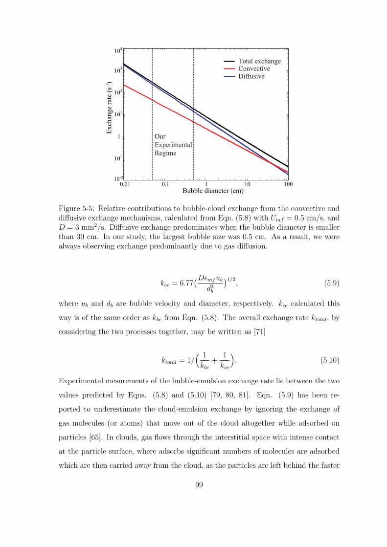
0.01 0.1 1 10 100
Bubble diameter (cm)
10-2
10
1
102
103
104
Exch
ange
rate
(s
)-1
-1
101
Total exchangeConvectiveDiffusive
Our
Experimental
Regime
Figure 5-5: Relative contributions to bubble-cloud exchange from the convective anddiffusive exchange mechanisms, calculated from Eqn. (5.8) with Umf = 0.5 cm/s, andD = 3 mm2/s. Diffusive exchange predominates when the bubble diameter is smallerthan 30 cm. In our study, the largest bubble size was 0.5 cm. As a result, we werealways observing exchange predominantly due to gas diffusion.
kce = 6.77(Dεmfub
d3b
)1/2, (5.9)
where ub and db are bubble velocity and diameter, respectively. kce calculated this
way is of the same order as kbc from Eqn. (5.8). The overall exchange rate ktotal, by
considering the two processes together, may be written as [71]
ktotal = 1/( 1
kbc
+1
kce
). (5.10)
Experimental mesurements of the bubble-emulsion exchange rate lie between the two
values predicted by Eqns. (5.8) and (5.10) [79, 80, 81]. Eqn. (5.9) has been re-
ported to underestimate the cloud-emulsion exchange by ignoring the exchange of
gas molecules (or atoms) that move out of the cloud altogether while adsorbed on
particles [65]. In clouds, gas flows through the interstitial space with intense contact
at the particle surface, where adsorbs significant numbers of molecules are adsorbed
which are then carried away from the cloud, as the particles are left behind the faster
99
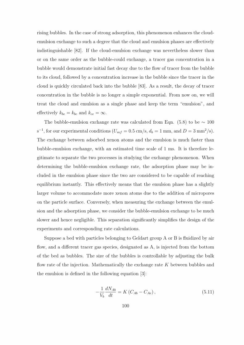
rising bubbles. In the case of strong adsorption, this phenomenon enhances the cloud-
emulsion exchange to such a degree that the cloud and emulsion phases are effectively
indistinguishable [82]. If the cloud-emulsion exchange was nevertheless slower than
or on the same order as the bubble-could exchange, a tracer gas concentration in a
bubble would demonstrate initial fast decay due to the flow of tracer from the bubble
to its cloud, followed by a concentration increase in the bubble since the tracer in the
cloud is quickly circulated back into the bubble [83]. As a result, the decay of tracer
concentration in the bubble is no longer a simple exponential. From now on, we will
treat the cloud and emulsion as a single phase and keep the term “emulsion”, and
effectively kbe = kbc and kce = ∞.
The bubble-emulsion exchange rate was calculated from Eqn. (5.8) to be ∼ 100
s−1, for our experimental conditions (Umf = 0.5 cm/s, db = 1 mm, and D = 3 mm2/s).
The exchange between adsorbed xenon atoms and the emulsion is much faster than
bubble-emulsion exchange, with an estimated time scale of 1 ms. It is therefore le-
gitimate to separate the two processes in studying the exchange phenomenon. When
determining the bubble-emulsion exchange rate, the adsorption phase may be in-
cluded in the emulsion phase since the two are considered to be capable of reaching
equilibrium instantly. This effectively means that the emulsion phase has a slightly
larger volume to accommodate more xenon atoms due to the addition of micropores
on the particle surface. Conversely, when measuring the exchange between the emul-
sion and the adsorption phase, we consider the bubble-emulsion exchange to be much
slower and hence negligible. This separation significantly simplifies the design of the
experiments and corresponding rate calculations.
Suppose a bed with particles belonging to Geldart group A or B is fluidized by air
flow, and a different tracer gas species, designated as A, is injected from the bottom
of the bed as bubbles. The size of the bubbles is controllable by adjusting the bulk
flow rate of the injection. Mathematically the exchange rate K between bubbles and
the emulsion is defined in the following equation [3]:
− 1
Vb
dNAb
dt= K (CAb − CAe) , (5.11)
100

where Vb is the bubble volume; NAb is the quantity of injected gas species A inside
the bubble; CAb is gas A concentration in the bubble and CAe is gas A concentration
in the emulsion. The emulsion-adsorption exchange rate is defined in a similar way,
being related to the tracer concentrations in the two phases.
5.2.6 Review of Conventional Methods
There have been two types of approaches to quantify the exchange behavior among
the different phases in a gas-fluidized bed: numerical simulations and experimental
measurements.
The simulation works apply the two-fluid model on the gas-fluidized granular
system, by considering the solid phase as the second fluid, in addition to the gas
phase, and the hydrodynamical behavior of the two phases are described by the
conservation of mass and momentum in each phase, together with the momentum and
energy exchange between the two fluids. Additional information about inter-particle
stress and internal momentum transfer in the solid phase is not readily available and
hence many assumptions are needed in order to solve the problem numerically. The
simulation approach is a mathematical challenge due to the large number of degree
of freedom in the solid phase, and as a result, the calculations require enormous
computational resources. Moreover, the simulation results are ultimately subject to
experimental verifications. The most recent simulation work on the bubble-emulsion
exchange yielded results in good agreement with Davidson’s predictions based on
Eqn. (5.8) [71], but it was only able to find the exchange rate between the emulsion
phase and a single bubble [83].
During the decade from the late 1960’s, there was enormous interest in measuring
experimentally the bubble-emulsion exchange rate in three-dimensional beds [80, 81,
84, 85]. In all of these measurements, the bubbles, on which the measurements were
performed, were generated by injecting a tracer gas at the bottom of the bed with
the rest of the bed in homogeneous fluidization regime, but at a flow rate close to
the point where bubbles would emerge. The injected bubbles were isolated from each
other and different from the naturally generated ones in another system where the
101

bed is in bubbling regime, which were small in size at the bottom of the bed and
grew bigger as they rose up the bed due to coalescence of multiple adjacent bubbles.
The flow patterns of the gas and solid phases induced by the bubble motions differed
from that in a regular bed with natural bubbles. Two different methods were used
to measure the exchange between these injected bubbles and the emulsion phase.
Stephens et al. [80] used a sampling tube to probe the tracer concentration in the
emulsion phase at different heights along the bed axis, from which they derived the
amount of gas exchange while the bubbles rose up in the bed. The procedure did not
account for the radial concentration gradient resulting from gas exchange out of the
bubbles, and as such, a significant systematic error exists in their results. Moreover,
the invasive probe tended to obstruct the flow path of the gas and particles, and
inevitably disturbed the bed operations, which may have caused unpredictable effects
on the exchange process. The second method was proposed by Chiba et al. [81], in
which an ultraviolet probe and spectrometer were used to detect tracer concentration
in the bubbles. The probe was installed in the bed so that there was a 1 cm gap at
the center of the probe to let bubbles pass through. This method was also invasive,
since the probe was installed inside the bed, and specifically it obstructed emulsion
flow, as well as disturbing bubble motion due to its close proximity to the bubbles.
In addition, they only measured the tracer concentration at a single point inside the
bubble, which was then assumed to be the tracer concentration in the entire bubble.
This assumption has been proved to be incorrect by later simulations [83].
Two additional limitations exist in the these measurements. First, they do not
account for the effect of the presence of multiple bubbles on the exchange rate. In a
natural bubbling bed, bubbles may interact with each other via frequent coalescence
and splitting, which may enhance the bubble-emulsion exchange rate. Secondly, the
size of the bubbles and their rising velocity were considered constant, which is gen-
erally incorrect. Bubbles provide a pathway for gas to flow through the bed with
less resistance, compared to the emulsion phase where large number of particles exist.
Consequently, the bubbles tend to expand by taking up emulsion gas, while rising
up through the bed [83, 85]. The increased bubble diameter results in a larger bub-
102

ble velocity. During the subsequent 30 years, no significant improvements have been
made on the experimental methodology.
The mass exchange between the gas and the solid particles is the second parameter
affecting the performance of a fluidized bed. It characterizes how efficiently the gas
molecules contact the solid surface, where the actual reaction happens. From the
early 1950’s to 1970’s, there were several experimental studies that measured the
gas-solid exchange rate by using various types of gas and particles [86, 87, 88, 89].
The method used in these studies is to introduce particles containing a removable
tracer material into a fluidized bed without any tracer initially. The tracer could
leave the solid phase by any of the following ways: sublimation, vaporization or
release from adsorption. The gas-solid exchange rate was measured by observing the
tracer concentrations in the inlet and outlet gas for the entire bed. This method,
however, was not able to provide information on the spatial dependence of the tracer
concentration along the bed. The method also relied on various assumptions and
empirical relations associated with bubble flow and gas exchange between bubbles and
the emulsion phase. Additionally, the preparation and conduct of these experiments
were extremely tedious and time-intensive. Moreover, no reported work of which we
are aware has been found that measures both the bubble-emulsion and emulsion-solid
exchange rates simultaneously.
Our experimental approach uses the NMR technique to non-invasively measure
the mass exchange rates among the different phases, including the bubble, emulsion
and adsorption phases in a gas-fluidized bed. The fast method developed in this study
enables us to probe the exchange behavior between the emulsion phase and multiple,
naturally generated bubbles, without assuming constant bubble diameter or homo-
geneous tracer concentration inside the bubble. It also allows us to simultaneously
measure the exchange rate between the emulsion gas and the solid phase, which is
distinguished by the large chemical shift due to the adsorption of xenon atoms.
103

5.2.7 The NMR Model
If we use spin magnetization, instead of injected gas concentration, the exchange
behavior may be equivalently described through the dynamics of the longitudinal
spin magnetization. Exchange occurs between bubbles and the emulsion phase, and
between the emulsion and adsorption phases. There is no direct exchange between
the bubbles and the adsorption phase, since the layer of gas around any single particle
belongs to the emulsion phase, and hence the gas molecules in bubbles need to traverse
the emulsion phase before they can be adsorbed. The gas flow and particle motions
were in the steady state. We minimized transient and unstable bed behavior by
supplying a steady and homogeneous gas flow from the bottom of the column, and
also by locating the RF coil at a high level up the bed so that the region from the bed
bottom to the RF coil is as long as possible. Moreover, the steady state condition was
guaranteed by extensive signal averaging, to smooth out the effects of any remaining
oscillatory flow behavior.
Spin magnetization may be manipulated with RF pulses and prepared in an initial
condition that can reveal their time-dependent motion in steady-state flow. The
temporal and spatial dependence of magnetization in the three phases can be written
as4
∂Mb
∂t+ ub
∂Mb
∂z= −kbe(Mb −Me)− Mb −M0
b
T b1
∂Me
∂t+ ue
∂Me
∂z= −ψb
ψe
kbe(Me −Mb)− kea(Me −Ma)− Me −M0e
T e1
(5.12)
∂Ma
∂t= −ψe
ψa
kea(Ma −Me)− Ma −M0a
T a1
Table (5.1) lists all the variables and their corresponding descriptions. These equa-
tions relate the material derivatives of spin magnetization in a fluid element along the
gas flow to different factors causing changes in their values. As an example, from the
equation for the dynamics of the emulsion magnetization, the term −ψb
ψekbe(Me−Mb)
4Clouds have been lumped into the emulsion phase.
104

Table 5.1: Descriptions of Variables Used in Eqn. (5.12)
Variable DescriptionMb Bubble magnetizationMe Emulsion magnetizationMa Adsorption magnetizationM0
b Bubble magnetization at thermal equilibriumM0
e Emulsion magnetization at thermal equilibriumM0
a Adsorption magnetization at thermal equilibriumub Bubble velocityue Gas flow velocity in the emulsion phaseψb Ratio of bubble volume to total bed volumeψe Ratio of emulsion gas volume to total bed volumeψa Ratio of micropore gas volume to total bed volumeT b
1 T1 in bubble phaseT e
1 T1 in emulsion phaseT a
1 T1 in adsorption phasekbe Bubble-emulsion exchange ratekea Emulsion-adsorption exchange rate
originates from the bubble-emulsion exchange; −kea(Me−Ma) is due to the emulsion-
adsorption exchange; while −Me−M0e
T e1
arises from T1 relaxation in the emulsion phase.
The gas velocity in the adsorption phase is zero since there is no net particle flow
in the steady state5. The volume ratios ψb, ψe, ψa are introduced to account for
different gas volumes in the three phases. These three equations are extensions from
Bloch’s Equation (2.11) to accommodate the exchange behavior as well as convective
gas flow.
The Xe NMR signal is sensitive to the volume integral of magnetization in the
sensitive region of the RF coil. We define the total magnetization, Mp, corresponding
to a phase labelled p as
Mp =
∫∫∫MpdVp = ψp
∫∫∫MpdV = ψpA
∫ z2
z1
Mpdz, (5.13)
5The circulation of particles throughout the bed causes mixing of the adsorption magnetizationalong the bed axis. However, since the particles are much less mobile compared to gas flow withnet particle flow being zero, we neglect the adsorption-phase flow term and considered the temporaland spacial dependence of Ma to be completely determined by the emulsion-adsorption exchange.
105

where ψp is volume ratio in phase p; A is the bed cross-sectional area; z1 and z2 are the
starting and ending positions marking the sensitive region of the RF coil; V is total
bed volume and Vp is the volume occupied by the phase. This representation is one-
dimensional along the flow direction, since distributions of the phases are considered
homogeneous in cross section [65]. Assuming the gas velocity in the bubbles and
emulsion phase do not change, we have the volume integral∫∫∫
dV on both sides of
Eqns. (5.12) as
1
ψb
dMb
dt+ ub(Mb|z2 −Mb|z1) = −kbe(
Mb
ψb
− Me
ψe
)− Mb −M0b
T b1ψb
1
ψe
dMe
dt+ ue(Me|z2 −Me|z1) = −ψb
ψe
kbe(Me
ψe
− Mb
ψb
)− kea(Me
ψe
− Ma
ψa
)
−Me −M0e
T e1 ψe
(5.14)
1
ψa
dMa
dt= −ψe
ψa
kea(Ma
ψa
− Me
ψe
)− Ma −M0a
T a1 ψa
.
In the NMR measurement of bubble-emulsion exchange, we initialized the mag-
netization so that at t = 0, polarized gas resided only in the region from the bottom
of the RF coil to the center of the RF coil. We also made sure that the front of
the gas flow did not reach the top of the coil during the measurement time. (See
Section 6.3 for detail) Moreover, we used the phase-cycling NMR technique to can-
cel the effects due to the advance of polarized gas into the RF coil region during
the measurement by averaging over multiple scans with alternating polarity in the
freshly entering magnetization. In the emulsion-adsorption exchange measurement,
the amount of gas flowing in or out of the RF coil only contributes to ∼ 0.2% of the
RF coil sensitive region during the measurement time. The inflow and outflow terms
in the above equations can therefore be ignored.
We performed 129Xe T1 measurement on a valved glass cell of aluminum oxide
particles, with the interstitial space filled by enriched 129Xe to 3 bars. Emulsion and
adsorption peaks were clearly resolved, and we were able to perform a T1 measurement
on them separately using the saturation recovery technique [90]. As a result, we
106

observed the same relaxation time in the two phases,
T obs1 = 44.0 s, (5.15)
due to the fast exchange between them. The observed relaxation time is related to
the intrinsic T1’s in these two phases, T e1 in the emulsion and T a
1 in the adsorption
phase, by
1
T obs1
=α
T e1
+1− α
T a1
, (5.16)
where α is the fraction of xenon in the emulsion phase. From Eqn. (5.16), we
immediately get T e1 > αT obs
1 and T a1 > (1 − α)T obs
1 . The value of α was measured
to be 0.612 (see section 6.4.2, where α = ψe/(ψe + ψa)), and we therefore can define
lower limits for T1 in the emulsion and adsorption phases:
T e1 > 26.9 s and T a
1 > 17.1 s. (5.17)
T b1 is not directly measurable but it should be comparable to that of bulk xenon,
which is at least on the order of tens of minutes. Compared to exchange rates kbe ∼100 s−1 and kea ∼ 1,000 s−1, T1 relaxation times for the three phases are much slower
and may thus be safely neglected. Based upon the above conditions, the dynamics of
the magnetization vectors M’s can be simplified as
dMb
dt= −kbe(Mb − ψb
ψe
Me)
dMe
dt= −kbe(
ψb
ψe
Me −Mb)− kea(Me − ψe
ψa
Ma) (5.18)
dMa
dt= −kea(
ψe
ψa
Ma −Me).
Bubble-Emulsion Exchange
Assuming time-independent ψb, ψe and ψa, with initial condition of
107

Mb(0) = M0b , Me(0) = Ma(0) = 0, (5.19)
Eqn. (5.18) has the following solution for the bubble magnetization:
Mb(t) = Ae−λ1t + Be−λ2t + C, (5.20)
where
λ1,2 = −1
2
[kea(1 +
ψe
ψa
)− kbe(1 +ψb
ψe
)
]± 1
2K, (5.21)
and
A = −kbe(1 + ψe
ψa− ψb
ψe+ ψb
ψa)− kea(1 + ψe
ψa)2 −K(1 + ψe
ψa)
2K(1 + ψe
ψa+ ψb
ψa)
M0b
B =kbe(1 + ψe
ψa− ψb
ψe+ ψb
ψa)− kea(1 + ψe
ψa)2 + K(1 + ψe
ψa)
2K(1 + ψe
ψa+ ψb
ψa)
M0b ,
C =ψb
ψb + ψe + ψa
M0b .
In the above equations, the symbol K is
K =
√[kea(1 +
ψe
ψa
)− kbe(1 +ψb
ψe
)
]2
+ 4kbekeaψb
ψe
.
If the exchange rate between the emulsion and adsorption phases is much faster
than that between the bubble and emulsion phases and the following condition is
true,
kea(1 +ψe
ψa
) À kbe(1 +ψb
ψe
), (5.22)
a Taylor-expansion of K yields the first order approximation,
K ' kea(1 +ψe
ψa
)− kbe(1 +ψb
ψe
) + 2kbe
ψb
ψe
1 + ψe
ψa
. (5.23)
108
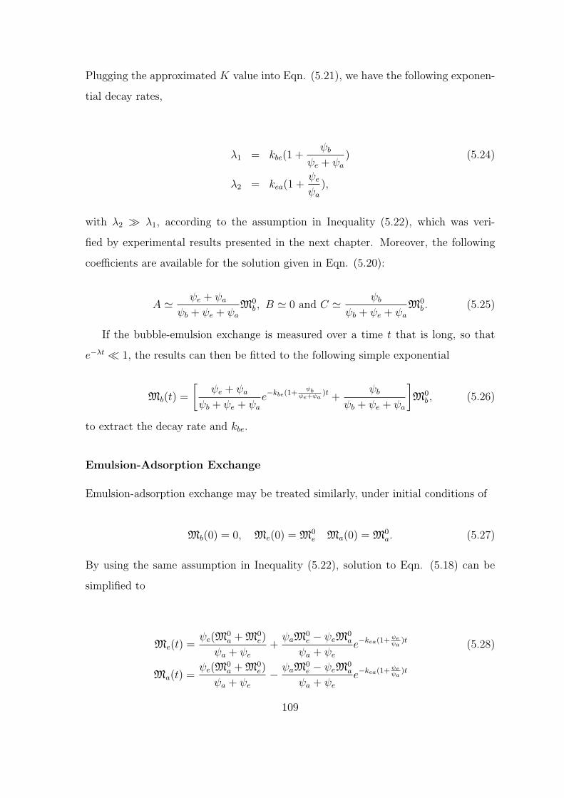
Plugging the approximated K value into Eqn. (5.21), we have the following exponen-
tial decay rates,
λ1 = kbe(1 +ψb
ψe + ψa
) (5.24)
λ2 = kea(1 +ψe
ψa
),
with λ2 À λ1, according to the assumption in Inequality (5.22), which was veri-
fied by experimental results presented in the next chapter. Moreover, the following
coefficients are available for the solution given in Eqn. (5.20):
A ' ψe + ψa
ψb + ψe + ψa
M0b , B ' 0 and C ' ψb
ψb + ψe + ψa
M0b . (5.25)
If the bubble-emulsion exchange is measured over a time t that is long, so that
e−λt ¿ 1, the results can then be fitted to the following simple exponential
Mb(t) =
[ψe + ψa
ψb + ψe + ψa
e−kbe(1+ψb
ψe+ψa)t +
ψb
ψb + ψe + ψa
]M0
b , (5.26)
to extract the decay rate and kbe.
Emulsion-Adsorption Exchange
Emulsion-adsorption exchange may be treated similarly, under initial conditions of
Mb(0) = 0, Me(0) = M0e Ma(0) = M0
a. (5.27)
By using the same assumption in Inequality (5.22), solution to Eqn. (5.18) can be
simplified to
Me(t) =ψe(M
0a + M0
e)
ψa + ψe
+ψaM
0e − ψeM
0a
ψa + ψe
e−kea(1+ ψeψa
)t (5.28)
Ma(t) =ψe(M
0a + M0
e)
ψa + ψe
− ψaM0e − ψeM
0a
ψa + ψe
e−kea(1+ ψeψa
)t
109

If proper initial conditions are generated as shown in Eqns (5.19) and (5.27),
we are able to measure the exponential decay rates of the bubble and adsorption
magnetization, from which the exchange rates kbe and kea may be calculated by fitting
data to the above two groups of solutions.
5.3 Conclusion
In conclusion, gas-fluidization is a complicated process that has been widely applied in
various industrial fields. The understanding of particle and gas dynamics in fluidized
granular systems is still under development. Our approach is to probe flow and
exchange dynamics by using hyperpolarized noble gas NMR, which has been successful
in studying gas flow in fixed porous media but never in fluidized granular media before.
The exchange behavior among the different phases has been described by using the
dynamics of the longitudinal magnetization in different phases. We will use this
description as an experimental model to measure the inter-phase exchange rates in
next chapter.
110

Chapter 6
NMR Study of Gas Dynamics in
Gas-Fluidized Granular Media
This chapter presents an NMR study of gas dynamics in a particle bed fluidized by
laser-polarized xenon gas. Previous NMR measurement of granular systems primarily
concentrated on the dynamics of the solid particles [91], which convey no direct infor-
mation about the gas dynamics. Direct NMR detection of the flowing gas will reveal
fundamental information about the gas dynamics, but the low signal-to-noise ratio
(SNR) obtained from thermally-polarized gases has made such measurements unfeasi-
ble. To address the problem of low SNR in gas-phase NMR, we use the spin-exchange
optical pumping method [92] to enhance the nuclear spin polarization of 129Xe gas by
3 - 4 orders of magnitude (compared to that available from the Boltzman distribu-
tion), producing a magnetization which can be as high as water samples at magnetic
field of ∼ 1 tesla. Our group has shown that in such as system, detailed studies of gas
flow dynamics in a variety of media is possible [21, 93, 94]. In this chapter, we report
results of variation in granular bed behavior in different fluidization regimes. These
are the first measurements to use NMR to non-invasively probe the emulsion gas and
gas bubbles; and to measure the exchange rates between the bubble, emulsion, and
adsorption phases.
Two important parameters, the inter-phase gas exchange rates, and the gas veloc-
ity distributions in the particle bed have been measured in our research. Aluminum
111

Polarizing
Cell with ~ 4 bar Xe
LaserLight
Polarized Xe
4.7 T Magnet Gradient Coil
Helmholtz Coils
VacuumPump
Natural
Abundance Xe
TEFLON tubing
Mass FlowController
Fluidized Bed Column
Polarizing
Cell with ~ 2.5 bar Xe
LaserLight
Polarized Xe
4.7 T Magnet Gradient Coil
Helmholtz Coils
VacuumPump
Natural
Abundance Xe
TEFLON tubing
Mass FlowController
Fluidized Bed Column
Figure 6-1: A schematic diagram of the Laser-polarized xenon - fluidized bed - NMRapparatus. Narrow 1/8 inch ID Teflon tubing connected the different sections of theapparatus, and provided the gas flow path. The tubing length was approximately2.5 m from the polarizer to the sample, and 5 m from the sample to the mass flowcontroller. The mass flow controller moderated the effect of the pump and determinedthe gas flow in the particle bed.
oxide (Al2O3) powders have a microporous surface that promotes xenon adsorption,
and this feature allows us to study the gas exchange between the emulsion and the
adsorption phases, in addition to gas exchange between the bubbles and emulsion.
The large magnetic susceptibility of the Al2O3 particles and their irregular shape
allows us to differentiate xenon bubbles from the emulsion and adsorption phases in
NMR spectroscopy using a T2-contrast method. Additionally, the large 129Xe chemi-
cal shift range allows the adsorption phase to be distinguished from the free gas. Our
experimental results demonstrated that the contrast methodology was successful in
distinguishing the various gas phases, and the exchange rates measured by this tech-
nique agree well with predictions from available models. We also measured the gas
velocity distribution using the pulsed-field-gradient method, which yielded velocity
distributions that clearly show the onset of bubbling and indirectly describe particle
motion in the fluidized bed.
112

6.1 Experimental Apparatus
6.1.1 Overview
Fig. 6-1 shows a schematic of the complete experimental apparatus. Xenon gas
(26.4% 129Xe) was spin-polarized in a glass cell which contained a small amount of
Rb metal. The total gas pressure was 2.5 bar, with the mixture consisting of 95%
xenon and the remainder N2. The cell was heated to 130◦C to create an appropriate
Rb vapor density to ensure spin polarization of the Rb vapor via optical pumping
on the Rb D1 line (∼ 795 nm). Circularly-polarized light for optical pumping was
supplied from ∼ 30 W of broad-spectrum (∼ 2 nm) light provided by a fiber-coupled
laser diode array. In a few minutes Rb-Xe collisions boost the 129Xe spin polarization
to ∼ 1% according to the calibration measurement mentioned in Chap 2.
Xenon gas flows from the polarizer through 1/8” I.D. Teflon tubing to the gas-
fluidized bed, with a pressure potential supplied by a vacuum pump located at the
end of flow path. The gas flow rate was regulated by a mass flow controller placed
just before the vacuum pump, which was capable of regulating steady flows ranging
from 10 to 1000 cm3/s. A continuous supply of polarized xenon gas, at a controlled
flow rate of 50-200 cm3 per minute (sccm), fluidizes the particle bed which is located
in an NMR magnet. The xenon gas pressure in the particle bed was measured to be
∼ 2.0 bar.
6.1.2 Fluidized Bed
As shown in Fig. 6-2, the fluidized bed setup used in the experiments consisted of
an 6 mm I.D. cylindrical Pyrex column, a windbox and two gas diffusers made of
porous Polyethylene (Porex Corp.) with a pore size of 2 micron. The windbox, with
its large volume, provided a buffer for the gas flow from the polarizer and the column.
On top of the windbox is the first gas diffuser, which ensures the vertical gas flow is
homogeneous in cross-section. The Pyrex column, located above the diffuser, served
as the container of the bed particles. A second diffuser covered the top of the column
113
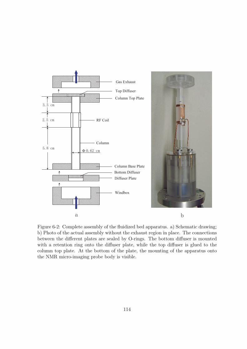
Windbox
Diffuser Plate
Column Base Plate
Column Top Plate
Gas Exhaust
Column
RF Coil
Φ
Bottom Diffuser
Top Diffuser
Figure 6-2: Complete assembly of the fluidized bed apparatus. a) Schematic drawing;b) Photo of the actual assembly without the exhaust region in place. The connectionsbetween the different plates are sealed by O-rings. The bottom diffuser is mountedwith a retention ring onto the diffuser plate, while the top diffuser is glued to thecolumn top plate. At the bottom of the plate, the mounting of the apparatus ontothe NMR micro-imaging probe body is visible.
114

Figure 6-3: Photos of the particles used in the fluidized-bed experiments, taken with100x microscope. a) Transparent glass beads sized between 45 and 70 µm, whichresults in them being classed as Geldart Group A particles. The beads are highlyspherical in shape. b) Opaque Al2O3 particles, sized between 75 and 104 µm, bypassing through appropriate sieves. These particles are classed as Geldart Group Band their shape is highly irregular.
to stop particles being carried out with the gas. The whole apparatus was assembled
with non-metallic materials to minimize spin depolarization of the laser-polarized
xenon gas transport. The fluidized bed apparatus was built on a standard vertical-
bore NMR micro-imaging probe body, to ensure accurate placement in the NMR
magnet. The probe body and connecting gas transport tubing was then positioned
in a 4.7 T vertical bore magnet, interfaced to a Bruker AMX2-based NMR console.
6.1.3 Particles
We chose two types of particles for this work: 45 ∼ 70 µm glass beads and 75 ∼104 µm aluminum oxide (Al2O3) powders1. Photo-micrographs of these particles are
shown in Fig. 6-3.
The glass beads are spherical while the shape of the Al2O3 particles is highly
irregular. The magnetic susceptibility of diamagnetic aluminum oxide is −37× 10−6
1The vendor of the glass beads is Jaygo Inc. The aluminum oxide powders were manufacturedby EM Science, with a part number of AX0612-1, and CAS number of 1344-28-1.
115

CM
CT
120°
Figure 6-4: Alderman-Grant RF Coil. The 120◦ RF windows were chosen for optimalfield homogeneity. CT and CM are tuning and matching capacitors which can beadjusted for optimal sensitivity at the 129Xe Lamor frequency.
cm3/mol, 25% larger than the value of magnetic susceptibility of glass. However, the
measured NMR linewidths of 129Xe flowing through the interstitial spaces of the two
types of particles are contrastingly different, with that from Al2O3 particles being 650
Hz (11.7 p.p.m.) while that from glass beads is on the order of 100 Hz (1.8 p.p.m.).
The irregularity in the shape of Al2O3 powders, which tends to introduce a stronger
heterogeneity in the magnetic field surrounding the particles, is likely the origin of
the broad linewidth.
6.1.4 Radio-Frequency Coil
Around the column is a homebuilt Alderman-Grant style RF coil [95], the design of
which is shown in Fig. 6-4. Copper foil tape was glued onto a 1/2” o.d. Teflon
tube to form the shape of the coil, and the tube made a tight fit around the fluidized
bed column. Although Alderman-Grant coils are not the best choice in terms of
field homogeneity across their total volume, since only their 60% is uniform, they are
sufficient for our experiments because the inner radius of the fluidized bed column is
less than 50% of the coil radius. The total sensitive length of the coil is 2.4 cm, which
116

Figure 6-5: 2D slice-selective images of a cylindrical water phantom 3 mm in diameterand 18 mm in length. a. X-Y plane image of a 1 mm thick slice, with a resolution of0.156 mm; b. Z-Y plane image of 2 mm-thick slice, with a resolution of 0.469 mm.
covers only a portion of the particle bed, without any free gas space beyond the two
diffusers or at the top of the column. This configuration eliminates possible artifacts
in NMR signals due to the inclusion of free gas in the sensitive region of the coil.
Fig. 6-5 shows 2D slice-selective images taken in both the X-Y and Z-Y planes,
the sample being a doped-water phantom inserted into the column. These images
demonstrate the good field homogeneity inside the column.
A similar fluidization apparatus has been designed for a horizontal-bore magnet
with the same field strength. Both the inflow and outflow tubings were bent 90◦ to
fit into the horizontal geometry. The RF coil was of solenoid type and capable of
generating decent homogeneous field. The figure of this setup is in Appendix B-1.
This first version of fluidization and NMR apparatus had two major problems. First,
the filling factor of the solenoid coil was only ∼ 6%, which resulted in fairly poor
SNR. Secondly, the sensitive region of the coil covered not only the particle bed, but
also the windbox below it, which generated a predominant narrow gas peak in the
spectrum and led to complications to data analysis. We therefore designed the second
117

system discussed above, with subsequent improvements on the two issues.
6.2 Optimizing Fluidized Bed Performance
6.2.1 Verification of Fluidization Apparatus
In a static bed without gas flow, solid particles experience no motion and the packing
pattern of these particles may be either random or ordered, depending on how these
particles were placed in the container. The shear stress among the particles originating
from particle weight keeps the system in a balance that is difficult to break without
external forces. The large bulk modulus of the solid particles results in a distribution
of the stress over distances much greater than the particle diameter, forming a force
chain that contributes to several interesting signatures in particle behavior during
fluidization. For example, the height of a bed of Geldart A particles exhibits hysteresis
as gas flow is cycled up and down across the homogeneous fluidization regime [96].
The phenomenon occurs because the particles are tightly jammed together in a fixed
bed, and in transition into fluidization, the force chain does not easily break without
large gas flow velocity in excess of that necessary for producing drag forces to support
the particle weight. Conversely, the inter-particle stress has been removed during
defluidization, and hence the gas velocity required to suspend the bed at the same
height is smaller.
Measurement of the hysteresis behavior in particle height was used to assess the
quality of the fluidization apparatus. A poorly designed fluidized bed, e.g., slightly
tilted (non-vertical) column, an ineffective windbox or a nonuniform diffuser, can
cause significant cross-sectional heterogeneity in gas flow and result in unpredictable
particle bed behavior. As a result, the hysteresis in particle height may disappear un-
der these circumstances. We therefore checked the column performance for problems
by observing hysteresis in the fluidization of glass beads.
Fig. 6-6 shows the measured particle bed height, observed visually, as a function
of gas flow rate2 at a constant gas pressure of 6.3 bar. Hysteresis was clearly observed
2Flow rate is measured in the unit “sccm”, or standard cubic centimeter per minute, which is
118

0 20 40 60 80 100 120 140
2
4
6
8
10
12
Flow rate (sccm)
Bed E
xpansi
on (
%)
FixedHomo-
geneousBubbling
Cycle up
Cycle down
Figure 6-6: Hysteresis in bed expansion, measured as a function of gas flow rate. DryN2 gas was used in this measurement. The particles are the glass beads with goodsphericity, and are classed as Geldart Group A particles. Homogeneous fluidizationwas therefore observable for these particles, with hysteresis apparent in this range offlow rates.
between the cycle-up and cycle-down tracks in the flow-rate range of 31 ∼ 64 sccm,
where the bed operated in the homogeneous fluidization regime. The results are
similar to those measured by Ojha et al. [96], and qualitatively verifies that our
experimental apparatus is capable of providing a reliable fluidization process.
6.2.2 Xenon Gas Pressure
As xenon is moderately expensive (∼ $8 - 10 per liter), optimizing xenon consump-
tion was a critical design consideration for these experiments . For some experiments,
despite the enhancements gained by optical pumping, several hours of NMR signal
averaging was required. During this time, the polarization system is ran in a continu-
ous flow mode. It was found that the amount of xenon required could be significantly
reduced by operating at the lowest possible gas pressure that still maintained the
fluidization state.
Fluidization of particle beds is only weakly dependent on gas pressure. For par-
the volume flow rate at STP.
119

1 2 3 4 5 6 7 810
20
30
40
50
60
70
80
Gas Pressure (bar)
Min
imu
m F
luid
izat
ion
Flo
w R
ate
(scc
m)
Figure 6-7: Dependence of minimum-fluidization flow rate Umf on gas pressure. Theuncertainty on the measured flow rates is 0.1 sccm. N2 gas was used to fluidize theglass beads. Data points were measured flow rates. The solid line is a linear fit.
ticles with diameter less than 100 µm, the minimum gas velocity that results in
fluidization, Umf , is independent of gas density [97, 1]. To verify this on our fluidized
bed setup, we measured gas flow rates corresponding to minimum fluidization at dif-
ferent gas pressures. The results are shown in Fig. 6-7. The flow rate measured is the
mass flow rate, which is proportional to gas density, the tube cross-sectional area, and
the flow velocity, Umf . The very good linear fit implies that Umf is independent of
gas pressure. The most significant parameter that controls which fluidization regime
the bed operates in is the gas flow velocity. Moreover, all the fluidization regimes are
found to be equivalently approachable with low pressure settings, and only insignifi-
cant changes in fluidization parameters have been observed as pressure was increased
[98]. It is therefore preferable to use reasonably low gas pressure so that the mass
flow rate, or the rate of gas consumption, is reduced, while the bed operates in the
same fluidization regime.
It is also important to account for the effect of xenon gas pressure on 129Xe spin
magnetization generated in the polarizer. The magnetization (and hence signal-to-
120

noise ratio) increases slowly with pressure3, placing a lower limit on an applicable
pressure value. We performed most NMR experiments with a gas pressure of 2.5 bar
in the polarization cell, which provided adequate signal strength and relatively light
xenon usage.
The pressure drop across the particle bed and the two gas diffusers was mea-
sured by two pressure gauges (26PC series by Honeywell, 100 psi maximum pressure)
mounted at the inlet and outlet of the bed. ∆P increased linearly with the gas flow
rate between 10 and 150 sccm. The pressure drop across a fluidized bed should be
independent of flow rate [1], and thus the measured ∆P is hence primarily due to
the two diffusers which provide a resistance to gas flow. The maximum pressure drop
was ∆P = 0.04 bar at flow rate of 150 sccm, only 5% of the average pressure in the
bed. Therefore, pressure variations throughout the particle bed could be neglected
at the 5% level.
6.3 Contrast Between Bubble and Emulsion Phases
In order to measure the exchange rate between the bubble phase and the emulsion
phase using NMR technique, the two phases need to be clearly differentiated. The
obvious difference between the bubble and emulsion phases is the concentration of
solid particles: the emulsion has a large particle number density (the total volume of
particles is ∼ 40%) while more than 99% of bubble volume is occupied by gas [1]. The
gas in close contact with solid particles tends to experience faster longitudinal and
transverse relaxation, and should therefore be distinguishable with NMR methods
via T1 or T2 contrast. Our experiments rely on the enhanced spin polarization to
acquire information on gas dynamics, and it is therefore implausible to use particles
containing T1 contrast agents that quickly diminish the spin polarization, resulting
in significantly reduced signal-to-noise ratio. We hence searched for methods that
utilize available T2 contrast.
3Magnetization is the product of density and spin polarization. In the case of laser-polarizedxenon, polarization decreases with xenon pressure due to the enhanced spin-rotation interactionbetween xenon and rubidium atoms [29].
121

Due to their high density, the magnetic susceptibility of solid particles is generally
three orders of magnitude larger than that of xenon gas. When both materials are
placed in a magnetic field of ∼ 1 T, magnetic susceptibility variations generate a
considerable magnetic field gradient at the boundary between the solid and gas phases.
The xenon gas spins in the emulsion phase thus tend to experience a much larger field
inhomogeneity than those in bubbles. Moreover, gas bubbles are almost spherical in
shape, and the resulting field inside the bubble will have a much higher homogeneity
than that in the emulsion phase. The NMR spectral line from the bubble thus should
be significantly narrower than that of the emulsion, providing a “contrast” between
the bubble and emulsion so that a measurement of the exchange rate between them
is possible.
Fig. 6-8 shows 129Xe spectra measured in an aluminum oxide particle bed, with
eleven different gas flow rates ranging from 15 to 125 sccm. The broad peak (∼ 650
Hz FWHM) at lower frequency is from xenon gas in the emulsion phase, and is the
result of the large field gradient in the interstitial spaces of the emulsion. There is
a slight shift in frequency of this peak away from that of free xenon gas. A second
broad peak with roughly the same width, but shifted 2.3 kHz, was identified as the
adsorption phase peak.
We measured the spectra at different gas flow rates in order to identify the narrow
peak (∼ 75 Hz FWHM) located on the shoulder of the emulsion peak. The peak
amplitude in Fig. 6-8 increased as the gas flow rate was raised from 15 to 125 sccm.
It is known that more bubbles appear, and they increase in size, as the gas flow
rate increases [99]. Based on the reasoning above that the magnetic field inside the
bubbles will be more homogeneous, due to lower magnetic susceptibility variations,
we identify the narrow peak as being from xenon in the bubbles. As the emulsion
peak is over an order of magnitude broader than the bubble peak, we predict that it
will be possible to differentiate the two phases unambiguously using NMR methods
to highlight the T2 contrast.
The spectrum was then acquired using the standard spin-echo pulse sequence
[12] with an echo time TE = 8 ms. The spectrum is shown in Fig. 6-9. Both the
122

−10 −5 0 5 10 15 20 25 30 350
5
10
15
20
25
Frequency (kHz)
Arb
itra
ry U
nit
1525
3545
5565
7585
95105
125 SCCM
12−8 −6 −4 −2 0 2 4 6 8 10
0
0.1
0.2
0.3
0.4
0.5
0.6
0.7
0.8
0.9
45 SCCM
Figure 6-8: Spectra of 129Xe in an Al2O3 particle bed, measured at 11 different gasflow rates (Fourier Transform of the acquired free-induction decays (FID) after a 90◦
hard pulse). The spectra were obtained by increasing the gas flow rate from 15 to125 sccm at gas pressure of 2.0 bar. The narrow peak is believed to originate fromthe bubble phase.
123

−10 −8 −6 −4 −2 0 2 4 6 8 10−1
0
1
2
3
4
5
6
−10 −8 −6 −4 −2 0 2 4 6 8 10−1
0
1
2
3
4
5
6
aSpectrum acquire with
a single RF pulse
b Spectrum acquire with
the contrast sequence
Figure 6-9: Spectra obtained from 129Xe gas fluidizing a bed of Al2O3 particles. a)The complete spectrum, acquired from a single RF pulse. b) The spectrum acquiredwith a spin-echo sequence, with an echo time of 8 ms. The spin-echo spectrum clearlyshows only the bubble peak, after removal of the emulsion and adsorption signals dueto spin decoherence during the echo time.
124

2
π
RF2
π
2
π
τ τ2
π
2
π
RF2
π
2
π
1 τ2
π
ττ3
Contrast
Generation Exchange Acqusition
Figure 6-10: The NMR pulse sequence used in bubble-emulsion exchange rate mea-surements. A π/2 hard RF pulse non-selectively flips spins into the transverse plane.After application of a π pulse, a spin-echo is generated after time τ1. τ1 was chosen tobe 8 ms, long enough for emulsion and adsorption magnetizations to decohere. Thebubble magnetization is then stored along the z direction following the second π/2pulse. Gas exchange between the bubble and emulsion phases occurs during the sub-sequent delay τ2. The third π/2 RF pulse then returns the remaining magnetizationback to the transverse plane, and the FID signal is acquired after a delay time τ3 of0.7 ms, which eliminates emulsion and adsorption magnetization that may have mi-grated from bubbles during τ2. Therefore, only 129Xe in the bubble phase contributesto the FID signal, which can be used to acquire useful exchange data.
emulsion and adsorption phase peaks disappear, due to gas diffusion in the presence
of the strong background gradient in these two phases. It is clear that the spin-echo
sequence worked effectively in suppressing the NMR signal from xenon in the emulsion
and adsorption phases.
Fig. 6-10 shows a pulse sequence that employs T2 contrast to remove the emulsion
and adsorption peaks from the spectrum, leaving only the bubble peak, so that we can
observe the time-dependence of the bubble magnetization and determine the bubble-
emulsion exchange rate. The experiment is a three-stage process: contrast generation,
exchange and acquisition.
Two factors may affect the bubble-emulsion exchange measurement. Bubbles are
continuously generated from the bottom of the particle bed and pass through the
bed with a velocity of ∼ 10 cm/s, corresponding to a time of 0.24 s for bubbles to
rise from the bottom to the top of the RF coil. During the exchange time τ2, more
bubbles may enter the coil region from below with freshly polarized 129Xe, and some
125

bubbles already in the RF coil region may exit the region at the top. The gas that is
entering and exiting gas have approximately equal volume but may have differing spin
polarization, resulting in a net accumulation of bubble magnetization during τ2. This
accumulation corresponds to the flow terms in Eqns. (5.14). To avoid this problem,
we phase-cycled the first 90◦ pulse and the receiver phase together, which alternatively
changed the polarity of the signal from the newly entering bubbles, and added together
the signals from all the scans. This resulted in the effective cancellation of NMR
signals from the newly arriving bubbles. (See Appendix D for details). A short pre-
acquisition delay (75 ms) was used before starting the sequence each time and 64
dummy scans were applied, so that the length of the particle bed region containing
polarized gas was approximately the product of the bubble velocity and the pre-
acquisition delay, or 7.5 mm. The maximum length of exchange time, τ2, was ∼100 ms, during which the polarized gas region moved 10 mm upward. Therefore,
the maximum length of the polarized gas region during the pulse sequence is 17.5
mm, which is less than the RF coil length (25 mm). Thus, the bubbles containing
polarized gas will stay inside the coil during the measurement. The implementation
of the experiment in this manner removes the flow terms in the differential equations
depicting magnetization dynamics (Eqn. (5.14)), significantly simplifing their solution
and making the comparison to experimental results much easier.
6.4 Measurement of the Bubble-Emulsion Exchange
Rate
6.4.1 Prediction of Bubble-Emulsion Exchange Rate
The estimation of the exchange rate between the bubble and emulsion phases re-
quires knowledge of the bubble sizes, as shown in Eqn. (5.8). Since the controllable
experimental parameter is the gas flow rate, we need to understand how the average
bubble size depends on gas flow rate. The size of a bubble size is directly related to
its velocity, as given by Eqn. (5.7), and we therefore used a two-phase flow model to
126

Ae
H
ub
Emulsion
Phase
Bubble
phase
Umf
U
Ab
ε mf
Figure 6-11: Two-phase flow model for gas flow in the bubble and emulsion phases. Ab
and Ae are cross-sectional area of bubble phase and the emulsion phase, respectively.H is the height of the particle bed. U is the total empty-tube gas flow velocity. εmf
is the void fraction in the emulsion phase.
determine the relation between bubble velocity and gas flow rate.
The flow velocity in the bubble phase is ub. The emulsion phase is assumed to stay
in the homogeneous fluidization state since changes in void fraction and interstitial
gas velocity in the emulsion are negligible as gas flow rate increases [65]. The void
fraction in the emulsion is therefore approximated by εmf , and the gas velocity by
Umf/εmf . The total gas flow velocity U is related to the flow rate q by the equation
U =T
T0
q
AP, (6.1)
where T is the gas temperature, which was 24◦ C for our experiment; T0 = 273.15
K; A is particle bed cross-sectional area which equals 0.302 cm2; and P is the gas
pressure measured to be 2.0 bar. We therefore have Umf = 0.541 cm/s, calculated
from Eqn. (6.1), given our experimental observation of qmf = 18 sccm.
127

Fig. 6-11 schematically depicts a model where inflowing gas is distributed into
the two phases. Given that the total volume flow rate should be equal to the sum of
the flow rates in the two phases, we have
UA = ubAb + UmfAe, (6.2)
where A is cross-sectional area of the whole bed; Ab and Ae are cross-sectional areas
taken up by the bubble phase and emulsion phase respectively. Obviously A = Ab+Ae.
The fraction of bed taken up by bubbles is
δ =Vb
V=
AbH
AH=
Ab
A, (6.3)
where Vb and V are bubble volume and total bed volume respectively; H is the bed
height. We hence relate the bubble volume fraction, δ, to the bubble velocity, ub, as
δ =U − Umf
ub − Umf
, (6.4)
From Eqn. (5.7) and (6.4), we can determine the bubble diameter by measuring
the bubble-induced bed expansion as a function of the gas flow rate, and then use
Eqn. (5.8) to determine the dependence of the bubble-emulsion exchange rate on the
gas flow rate. The expansion of the fluidized bed, E, is related to bubble fraction, δ,
by
E =δ
1− δ. (6.5)
The emulsion phase also expands as flow rate increases, exhibiting increased inter-
particle distance, but this expansion is minimal compared to that due to bubble
formation, and can be neglected, especially for Geldart Group B particles [65]. This
approximation is consistent with the previous assumption that the emulsion phase
may be considered to always be in a state equivalent to minimum fluidization [1]. Eqn.
(6.4) has been verified by Orcutt, Davidson and Pigford, who used it to estimate the
bubble diameter [100]. It has also been used by Menon and Durian [62] in their
128

20 40 60 80 100 120 140 1600
5
10
15
20
25
30
35
40
45
Per
cen
tag
e E
xp
ansi
on
(%
)
Gas flow rate (SCCM)
a
0 20 40 60 80 100 120 140 1600
0.5
1.0
1.5
2.0
2.5
3.0
3.5
4.0
Gas Flow Rate (SCCM)
Bu
bble
Dia
met
er (
mm
)
b
Figure 6-12: Measured particle bed expansion (a) and estimated bubble diameter (b)as functions of gas flow rates. The size of the bubbles increases monotonically withthe flow rate. At 160 sccm, the bubble diameter is greater than 60% of the columninner diameter, indicating that the fluidization is approaching the slugging regime.This was confirmed by visual inspection of the bed at that flow rate.
experimental studies, where they used 96 µm glass beads, close to our particle size4.
The approximation that the emulsion volume expansion negligible will be validated
in section 6.4.2.
By visually studying the particle bed surface, we measured the percentage expan-
sion of the aluminum oxide bed as the gas flow rate was increased from 0 to 150 sccm,
at which point the bed started to demonstrate slugging behavior. Fig. 6-12 shows the
result of this measurement. The total volume of the particle bed occupied by bubbles
varies even at a constant gas flow rate, since both the number of bubbles and average
bubble size fluctuate. We therefore measured the average value of the expansion by
observing the top of the particle bed for 30 seconds, a time much longer than the
time scale for the fluctuation. The average bubble diameter was then calculated by
using the equations (6.4), (6.5), (5.7) and U = q/AP . Similarly Umf is related to the
flow rate corresponding to the onset of fluidization.
Using Eqn. (5.8) and the calculated bubble diameters, we predicted the bubble-
emulsion exchange rate kbe, as shown in Fig. 6-13. As the flow rate increases, the
4Menon and Durian used approximation E ≈ δ, based on the experimental condition that bubblevolume was much smaller than that of the whole bed, i.e. δ ¿ 1. Moreover, ub was considered muchlarger than Umf and therefore ub − Umf ≈ ub.
129

40 60 80 100 120 140 16010
20
50
100
200
500
1000
Gas Flow Rate (SCCM)
Bu
bb
le−
Em
uls
ion E
xch
ang
e R
ate
(s )
-1
Figure 6-13: Predicted bubble-emulsion exchange rate. Since 35 sccm was the pointwhere we started to observe a bubble peak in the 129Xe NMR spectra, it was the lowestflow rate where bubble-emulsion exchange could be measured. Thus the predictioncurve does not extend to flow rates below 30 sccm. The exchange rate is plotted ona logarithmic scale.
average size of the bubbles gets larger, since more inflowing gas enters the bubble
phase and the coalescence of adjacent bubbles is enhanced. The exchange rate for
larger bubbles is expected to be smaller, since it takes longer to replenish gas in a
larger bubble. The exchange rate was found to be strongly dependent on the flow
rate, for the range 30 and 75 sccm, but weakly dependent when the flow rate is faster
than 75 sccm.
6.4.2 Determining Ratios of Void Fractions in Different Phases:
ψb/ψa and ψe/ψa
Eqn. (5.26) relates the bubble-emulsion exchange rate to the decay rate of bubble
magnetization measured with the pulse sequence shown in Fig. 6-10, giving
k = kbe(1 +ψb
ψe + ψa
), (6.6)
130

Arb
itra
ry U
nit
Arb
itra
ry U
nit
−10 −8 −6 −4 −2 0 2 4 6 8 10
0
0.1
0.2
0.3
0.4
0.5
0.6
0.7
0.8
0.9 105 SCCM
−10 −8 −6 −4 −2 0 2 4 6 8 10
0
0.1
0.2
0.3
0.4
0.5
0.6
0.7
0.8
0.9
35 SCCM a b
Figure 6-14: Peak deconvolution in 129Xe spectra obtained from xenon gas fluidiz-ing Al2O3 particles. Deconvolution was achieved by fitting to three independentLorentzians. a) spectrum measured at flow rate of 35 sccm, with a small bubblevolume. b) spectrum at flow rate of 105 sccm, with a large fraction of the gas in thebubble phase. The circles in the two plots label the measured spectra, and the linesare fitting results.
where k is the exponential decay rate of the bubble magnetization. We determined
the coefficients ψe and ψa, respectively, the volume percentage occupied by emulsion
and adsorption phases, before calculating the value of kbe from k.
ψe/ψa is equivalent to the ratio of the emulsion and adsorption magnetization,
which are given by integrals of the two peaks in 129Xe spectra. However, direct
integration of the emulsion and adsorption peaks was difficult due to the overlap of
the two broad peaks. Moreover, the bubble peak was on the shoulder of the emulsion
peak, resulting in fairly complicated spectra. To address this problem, we fitted the
spectra to the sum of three Lorentzian curves to separate the contributions from the
different components. Fig. 6-14 shows the results of the curve fitting on the spectra
measured at 35 and 105 sccm respectively.
We integrated the emulsion and adsorption peaks in each spectrum, and calculated
the ratio between them to yield ψe/ψa, as shown in Fig. 6-15. When these spectra
were acquired, a dead time was used between the end of the RF excitation pulse
and the start of data acquisition, to allow for coil ring down. The emulsion and
adsorption magnetization were both attenuated during the dead time, the amount of
attenuation being related to their transverse decoherence times T ∗2 . Since the observed
131

0 20 40 60 80 100 120 1401. 0
1. 1
1. 2
1. 3
1. 4
1. 5
Flow Rate (SCCM)
ae
ψ /
ψ
1.581 ± 0.044
Figure 6-15: Plot of the ratio of emulsion phase to adsorption phase volume, ψe/ψa
as a function of gas flow rate. ψe/ψa was seen to be independent of flow rate, anddetermined to be 1.581 ± 0.044. The error bars were estimated from the noise levelin the spectra.
T ∗2 ’s associated with the two peaks were the same based on linewidth measurements,
their attenuations were of the same amount and did not affect the calculation of
ψe/ψa.
No dependence of ψe/ψa on the flow rate has been observed, even though the
measured variations around the average value, 1.581 ± 0.044, were observed. The
volume of the adsorption phase is directly related to the micropore volume of the
particles, which is flow-independent given a constant temperature and gas pressure.
ψa is hence proportional to the volume of the solid phase and the porosity of the
particles. The ratio ψe/ψa therefore reflects the ratio of interstitial volume to solid
volume, and is a measure of the expansion of the emulsion phase as a function of flow
rate. This result confirms that expansion in the emulsion phase is negligible for the
Geldart Group B particles used in our measurement.
We therefore conclude that the ratio of emulsion gas volume to adsorption gas
volume is independent of the gas flow rate and simply use the average value
132

10 20 50 100 2000
0.2
0.4
0.6
0.8
1.0
Flow Rate (SCCM)
ab
ψ /
ψ
Figure 6-16: Plot of the dependence of ψb/ψa on gas flow rate, which is plotted hereon a logarithmic scale. The ratio steadily increases with flow rate, consistent withthe knowledge that bubble volume increases steadily with gas flow rate. The errorbars were estimated from the noise level in the spectra.
ψe
ψa
= 1.581± 0.044 (6.7)
for the rest of the thesis.
Calculation of the exchange rates also requires knowing the ratio ψb/ψa, which
can also be determined available from the spectra of gas-phase 129Xe fluidizing the
Al2O3 particles. Using the same peak deconvolution from Fig. 6-14, we integrated
the bubble and adsorption peaks and calculated the ratio Rba. Accounting for the
dead time, τ = 0.5 ms, between the end of the π/2 pulse and the beginning of data
acquisition, and the transverse relaxation times in the two phases, T ∗2b = 4.4 ms and
T ∗2a = 0.50 ms measured with the CPMG sequence, we calculated ψb/ψa
ψb
ψa
=e− τ
T∗2a
e− τ
T∗2b
Rba. (6.8)
Rba was determined from nine different spectra acquired at flow rates throughout
the bubbling fluidization regime, and the resultant ψb/ψa values are given in Fig. 6-
133

16. The flow rate is plotted on a logarithmic scale, and a linear fit of the data points
gives the following relationship between the two parameters:
ψb
ψa
= −2.1862 + 0.6446 log q, (6.9)
which is a useful empirical relation for finding the value of ψb/ψa at any flow rate.
The correlation coefficient R2 (see Appendix E for definition) associated with the
linear fitting was found to be 0.962, representing a good linear relationship. Fig. 6-16
indicates the volume fraction occupied by bubbles in the bed increased as flow rate
went up.
Note that the measurement of bubble volume by the spectroscopy method was
not accurate when the bed was just above the minimum fluidization condition, i.e.,
at flow rates between 18 and 35 sccm. The bubble-emulsion contrast mechanism is
not effective when the bubble size is similar to the particle size. From Fig. 6-12,
we can see that the bubble diameter at such flow rates is < 0.2 mm, or less than
two times the particle diameter. In this case, the contrast in field homogeneity is
weak and the bubble peak may not be observable. This explains the extremely low
bubble peak amplitude at flow rate below 35 sccm, even though a significant amount
of bubbles were seen by visual inspection.
The ψe/ψa and ψb/ψa values at different flow rates were then used in relating the
experimental data to the actual exchange rates, with interpolation or extrapolation
applied if necessary.
6.4.3 NMR Results
We measured the xenon exchange rate between the emulsion and bubble phases using
the pulse sequence shown in Fig. 6-10, with a series of values for the exchange
time, τ2, ranging from 1 to 50 ms. Nine different gas flow rates between 35 and
150 sccm were used. Fourier-Transformation of the FID signals yield post-exchange
129Xe spectra containing only the bubble peak, which was integrated to determine the
bubble magnetization. The time-dependence of the bubble magnetization, together
134

0 5 10 15 20 25 30 35 40 45 500.5
0.6
0.7
0.8
0.9
1.0
1.1
1.2
Am
pli
tude
(A.U
.)
Bubble Exchange Time τ (ms)
0.4
0.5
0.6
0.7
0.8
0.9
1.0
Am
pli
tude
(A.U
.)
k = 180.8E36.0 s
40 SCCM
0 5 10 15 20 25 30 35 40 45 50Bubble Exchange Time τ (ms)
-1be
k = 64.3E13.0 s
60 SCCM -1
be
22
Figure 6-17: Decay of bubble magnetization at 15 different exchange times, τ2, andtwo different flow rates: 60 and 40 sccm. The exponential fits yield decay rates thatwere related to bubble-emulsion exchange. 256 signal-averaging scans were used foreach acquisition, and the resulting signals coherently added to reduce variations inthe bubble amplitude. The delay times used in the sequence were: contrast delaytime, τ1 = 8 ms, exchange time, τ2, varied between 1 and 50 ms, pre-acquisition delayτ3 = 0.7 ms.
with a fitted exponential curve, is plotted in Fig. 6-17 for two selected flow rates.
At both flow rates, the data fit to a single-exponential, indicating no evidence of
recirculation of gas between the bubbles and their surrounding cloud. The variation
in the results measured at 40 sccm was due to statistical errors resulting from small
number of detectable bubbles. The number of bubbles in the coil-sensitive region of
the particle bed was estimated to be about 30. The generation and coalescence of
bubbles are uncontrollable random processes, resulting in variations in the number
of bubbles in the particle bed at any instant of measurement. When the bed is
initially fluidized, fewer bubbles exist and more significant variations are expected.
This statistical error is the major contributor to the uncertainties in the exchange
rate measurements.
The exponential decay rate of bubble magnetization is related to the exchange
rate according to Eqn. (6.6), and can be equated to:
k = kbe(1 +ψb
ψe + ψa
) = kbe(1 +ψb/ψa
1 + ψe/ψa
). (6.10)
135

40 60 80 100 120 140 16010
20
50
100
200
500
1000
Bubble−Emulsion Exchange Rate (s ) Prediction
NMR Results
-1
Flow Rate (SCCM)
Figure 6-18: Measurements of the bubble-emulsion exchange rate. The predictedcurve from Fig. 6-13 is included for comparison. 256 signal averaging scans weresummed in each measurement to reduce statistical errors. The exchange rate is plottedon a logarithmic scale.
By using the values of ψb/ψa and ψe/ψa determined in the last section, we found the
following correlation between k, kbe and flow rate q
k = (0.1530 + 0.2497 log q)kbe, (6.11)
which allows the bubble-emulsion exchange rate to be calculated as a function of flow
rate. A plot of this data is shown in Fig. 6-18.
The measured exchange rates agree well with the prediction curve, which was
derived in section 6.4.1 and was based on limited information and several assumptions.
The large uncertainty in the data at 35 sccm is due to statistical errors resulting from
the small number of bubbles found in the bed at this flow rate. The measured rates
are smaller than the prediction for flow rates below 60 sccm, and the discrepancy may
be explained by the presence of the cloud phase. In the development of the model
136

used to derive the predicted curve, we included the cloud phase in the emulsion,
assuming the exchange between the two is much faster than that between bubbles
and their clouds. Recirculation of polarized gas back into the bubbles, which would
effectively reduce the exchange between the cloud and the emulsion, resulting in the
lowered overall exchange rate. Therefore, the neglected cloud phase is one possible
reason for the discrepancy.
Aside from the minor discrepancy, the prediction based on Davidson’s model
agrees well with the experimental data. The measurement verifies that this model
may be safely used in predicting bubble-emulsion exchange rates in the design of
fluidized beds.
6.5 Measurement of the Emulsion-Adsorption Ex-
change Rate
The bubble-emulsion exchange was measured assuming the exchange between the
emulsion and adsorption phases is much faster and the two phases were indistinguish-
able. Conversely, emulsion-adsorption exchange can also be measured if we consider
kbe to be very slow, and therefore negligible. The exchange is limited by gas diffusion
in the interstitial spaces of the emulsion, and in Section 5.2.4, the time scale for this
diffusion was estimated to be ∼ 1 ms.
We designed a pulse sequence, that is similar to teh standard saturation-recovery
experiment, to undertake this measurement of emulsion-adsorption exchange. The
sequence is shown in Fig 6-19.
The selective saturation pulses only cover the frequency range of the adsorption
peak, but leaves the magnetization in the emulsion phase unperturbed. The selective
pulses were not expected to completely spoil the adsorption magnetization since the
length of the pulse itself is ∼ 1 ms, which is on the same order as the expected
emulsion-adsorption exchange time. A certain amount of adsorption magnetization
remains after the selective pulses, but the balance between the two phases has been
137

τ
Selective saturation of adsorption phase
Adsorption recovery
FID detection
RF
Selective saturation of adsorption phase
Adsorption recovery
FID detection
2
π
2
π
Figure 6-19: NMR pulse sequence used to measure the emulsion-adsorption exchangerate. Three π/2 selective pulses were used to rotate the adsorption magnetizationinto the transverse plane repeatedly, so that the magnetization balance between thetwo phases was disturbed. The separation between any two soft-pulses is 1.0 ms,of the same order as the transverse relaxation time of the adsorbed phase, T a
2 . Adelay time, τ , was then used to allow exchange to occur between the adsorbed andemulsion phases. Spins exchanging in from the emulsion phase retain their high spinpolarization. τ was varied in our experiments from 0.1 to 10 ms. Finally a non-selective π/2 RF pulse allowed sampling of magnetization components in all phases,after exchange.
138
disturbed. We were able to measure the exchange rate by observing the rate at which
the adsorption magnetization was recovered from this perturbation.
We used a similar curve fitting and peak deconvolution technique mentioned in
previous section to resolve overlapping peaks, and performed an integration over the
adsorption peak to retrieve adsorption magnetization after different delays, τ . Fig.
6-20 shows one of the spectra, measured at 60 sccm. The spectral line was fitted to
three Lorentzians, and then the bubble and emulsion peaks were subtracted. Next an
exponential fitting was applied to find the adsorption peak decay rate k′. According
to Eqn. (5.28), k′ is related to the emulsion-adsorption exchange rate kbe by
k′ = kea(1 +ψe
ψa
), (6.12)
where ψe
ψa= 1.581. The resultant kea values measured as a function of gas flow rate
are shown in Fig. 6-21. The value of kea scatters around an average value of 388
s−1, and no obvious dependence on gas flow rate is observed. kea is related to the gas
diffusion in the interstitial space only, as the Peclet number is much less than one for
all flow rates used. Additionally, as we showed in Section 6.4.2, the expansion of the
emulsion phase is negligible and as such the inter-particle distance in the emulsion
is considered independent of flow rate. Therefore, the time for a gas molecule to
traverse the interstitial space in the emulsion remains constant, and hence k′ should
be independent of flow rate. The experimental results are in agreement with this
theoretical understanding.
The apparent decay rate kbe(1 + ψb
ψa+ψe) for bubble-emulsion exchange is an order
of magnitude slower than the rate kea(1+ ψe
ψa) for emulsion-adsorption exchange. This
verifies the assumption of Inequality (5.22), made in the last chapter, for decoupling
the two exchange processes and considering them isolation.
6.6 Error Analysis
We estimated uncertainties in the NMR measurements of the exchange rates by error
propagation of the uncertainties in the NMR signal amplitudes and their integrations,
139

−10 −8 −6 −4 −2 0 2 4 6 8 10
0
0.2
0.4
0.6
0.8
Frequency (Hz)
-5 0 5 10 15 20 25 30 35Frequency (Hz)
0
1
2
3
Am
pli
tude
(A.U
.)
τ = 0.1 ms
0.5 ms
1.1 ms
5 ms
Am
pli
tude
(A.U
.)
a
b
Bubble
Emulsion
Adsorption
Figure 6-20: (a) A single 129Xe spectrum measured at a gas flow rate of 60 sccm, alongwith deconvoluted spectra for each component derived from fitting the main spectrawith three Lorentzians. (b) The derived spectra for the adsorption peak only, aftersubtraction of the fitted bubble and emulsion components measured at 16 differentexchange times, τ . The ripples around zero frequency are the result of imperfectsubtraction of the much larger bubble peak. The amplitude of the adsorption peakincreases slowly with the exchange time, τ , which was used to find the exchange time.
140
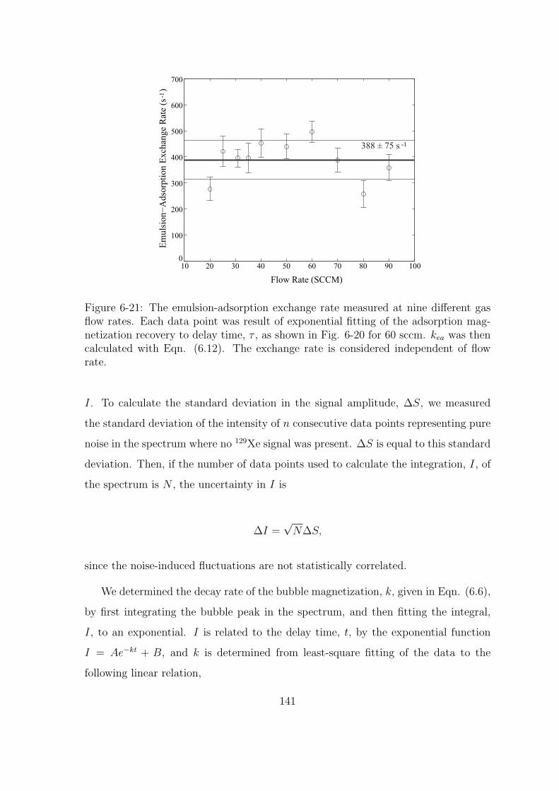
10 20 30 40 50 60 70 80 90 1000
100
200
300
400
500
600
700
Flow Rate (SCCM)
Em
uls
ion
−A
dso
rpti
on
Exch
ang
e R
ate
(s )
-1
388 ± 75 s -1
Figure 6-21: The emulsion-adsorption exchange rate measured at nine different gasflow rates. Each data point was result of exponential fitting of the adsorption mag-netization recovery to delay time, τ , as shown in Fig. 6-20 for 60 sccm. kea was thencalculated with Eqn. (6.12). The exchange rate is considered independent of flowrate.
I. To calculate the standard deviation in the signal amplitude, ∆S, we measured
the standard deviation of the intensity of n consecutive data points representing pure
noise in the spectrum where no 129Xe signal was present. ∆S is equal to this standard
deviation. Then, if the number of data points used to calculate the integration, I, of
the spectrum is N , the uncertainty in I is
∆I =√
N∆S,
since the noise-induced fluctuations are not statistically correlated.
We determined the decay rate of the bubble magnetization, k, given in Eqn. (6.6),
by first integrating the bubble peak in the spectrum, and then fitting the integral,
I, to an exponential. I is related to the delay time, t, by the exponential function
I = Ae−kt + B, and k is determined from least-square fitting of the data to the
following linear relation,
141

lnI −B
A= −kt,
and the uncertainty of the fitted k value is given by (see Appendix E or [53])
∆k = T 22
√√√√ 1
∆
n∑i=1
1
σ2i
,
where σi and ∆ are
σi =∆Ii
Ii −B,
∆ =n∑
i=1
1
σ2i
n∑i=1
t2iσ2
i
−( n∑
i=1
tiσ2
i
)2
,
in which Ii is the integral of the spectrum measured after the delay time, ti. The
uncertainty in the bubble-emulsion exchange rate, kbe, is therefore given by
∆kbe = kbe
√√√√√(∆k
k
)2
+[∆
(ψe
ψa
)
1 + ψe
ψa
]2
+[∆
(ψb
ψa
)(
ψb
ψa
)]2
, (6.13)
where ∆(
ψe
ψa
)is given in Eqn. (6.7) and ∆
(ψb
ψa
)is determined by calculating the
standard deviation of the data points shown in Fig. 6-16, subtracted from the fitting
result given in Eqn. (6.9).
The uncertainty in the emulsion-adsorption exchange rate was calculated using
the same method.
6.7 Gas Velocity Measurement
We have also measured the gas flow velocity in a fluidized bed with the pulsed-
gradient stimulated echo (PGSTE) sequence. Seven different gas flow rates were used
to observe the effect of flow rate changes on gas velocity distribution. Glass beads
of 50 µm in diameter were used in this measurement. They provide a higher NMR
142

-3 -2 -1 0 1 2
0.0
0.1
0.2
0.3
0.4
0.5
0.6
0.7
0.8
0.9
1.0
Rel
. p
rob
abil
ity
(A
.U.)
Velocity (cm/s)
75 sccm (1.14 cm/s)50 sccm (0.758 cm/s)
40 sccm (0.607 cm/s)30 sccm (0.455 cm/s)
-3 -2 -1 0 1 2
0.0
0.1
0.2
0.3
0.4
0.5
0.6
0.7
0.8
0.9
1.0
Rel
. pro
bab
ilit
y (
A.U
.)
Velocity (cm/s)
10 sccm (0.152 cm/s)16 sccm (0.243 cm/s)
21 sccm (0.319 cm/s)30 sccm (0.455 cm/s)
Figure 6-22: Xenon gas velocity distributions measured in two fluidization regimes.50 µm glass beads were fluidized by laser-polarized xenon. Velocity spectra weremeasured by the pulsed field gradient stimulated echo technique, in which the gradientpulse duration, d = 1 ms, the flow encode time D = 10 - 1000 ms and the maximumgradient pulse strength was 20 G/cm. a). Four different gas flow rates: 10, 16, 21and 30 sccm were used, all of which ensured the particle bed was in the homogeneousfluidization regime. b). Similar measurements made at three higher gas flow rates:40, 50 and 75, corresponding to the bubbling fluidization regime. Also included is thedata for 30 sccm, the transition point between homogeneous and bubbling fluidization.The superficial gas velocities corresponding to the flow rates are given in parentheses.
signal since the Xe spectral peak is an order of magnitude narrower with the alumina
particles. The results of the measurement are shown in Fig. 6-22. When the gas
flow rate was below 30 sccm, the particle bed was in the homogeneous fluidization
regime, in which our previous measurements show that the movement of particles is
minimal and the gas percolates through the interstitial spaces in the laminar flow
regime. This is verified by the results shown in Fig. 6-22 a), where the average
velocity increases with gas flow rate but the broadness of the distribution, a measure
of random dispersion, is independent of flow rate.
Fig. 6-22 b) shows the velocity distributions at flow rates above 30 sccm, where
the particle bed is in the bubbling fluidization regime. As as result of bubble for-
mation and movement, particle motion now occurs. This motion changes the flow
paths continuously, and therefore increases gas dispersivity. The velocity distribution
corresponding to 30 sccm is also included for comparison. The width of the peaks
increased with gas flow rate, indicating more random gas flow patterns related to
143
bubble-agitated particle motion. Surprisingly, the average gas velocity was seen to
decreased at higher gas flow rates in this regime. We believe the reason for this is
that the bubble velocity was larger than the maximum velocity detectable with this
method. A larger portion of gas entered the bed in form of bubbles at a higher gas
flow rate, and left the bed without being detected, resulting in a decreased observed
average gas velocity.
144

Chapter 7
Discussion of Fluidized-Bed
Experiments
7.1 Verification of Assumptions
The experimental study presented in Chapter 6 attempted to characterize the complex
gas-phase dynamics of a gas-fluidized bed. The underlying theoretical model and the
execution of the experiments were based on several assumptions that helped reduce
the complexity of the problem but still captured the essence of the complex flow. In
this chapter we review the main assumptions made in the earlier two chapters and
assess their justification.
7.1.1 Merging Cloud and Emulsion Phases
The clouds exist around every single bubble, between the bubble and emulsion phases.
In development of the model described in Section 5.2.5, we assumed that the gas
exchange rate between clouds and the emulsion phase is much faster than the bubble-
cloud exchange so that the recirculation of gas immediately back into bubbles is
negligible, owing to the substantive gas adsorption and fast exchange between inter-
stitial gas and adsorbed atoms. We hence lumped clouds into the emulsion phase,
with the additional justification that they are both particle-dense phases.
145

Cloud
Emulsion
Gas
Recirculating
pathway in
the cloud
ub
ub -Umf
Figure 7-1: Recirculation of gas through a bubble. The circulating gas penetrates thedense cloud around the bubble. The particles surrounding the bubble are assumedto have negligible velocity compared to the bubble rising velocity ub, according toDavidson’s bubble model. The thick curve on the left shows the flow path of therecirculating gas which moves with velocity ub−Umf , relative to the emulsion phase.
146

Fig. 7-1 depicts the gas flow patterns around a bubble rising upwards in the
fluidized bed with a velocity ub, through the emulsion phase. According to Davidson’s
bubble model [71], the rising bubbles push aside the particles which behave like an
incompressible inviscid fluid, and the velocity of the particles is therefore negligible
compared to ub. Moreover, the recirculating gas flows with a velocity ∼ Umf ¿ ub
relative to the quasi-static emulsion, so we estimate the gas flow velocity in the cloud
to be ub − Umf ' ub. In the measurement of the bubble-emulsion exchange, the
initial xenon magnetization in both the emulsion and adsorption phases was zero, so
the recirculating gas continuously encountered the emulsion and adsorption phases
with no hyperpolarization. As a result, the ratio of decrease in magnetization of gas
reentering the bubble is estimated to be
e− db
ubτ ' 0, (7.1)
where db is the bubble diameter and τ is the exchange time between the interstitial
gas and adsorption phase, being on the order of 1 ms. The approximation was based
on the condition of the typical bubble diameter of 2 mm and the corresponding ub of
10 cm/s. To summarize, the reentering gas has zero polarization and the exchange
between the cloud and the emulsion phase outside the cloud is fast enough so that
the cloud layer places no impedance on the bubble-emulsion exchange. It is therefore
justified to use the bubble-cloud exchange rate kbc to approximate the exchange rate
between the bubble and emulsion phases.
Fig. 7-2 shows the predicted time-dependence of spin magnetization within the
bubble phase with and without adsorption of gas on the particles. In the case of
no adsorption, the recirculation of hyperpolarized gas results in a later increment of
the bubble magnetization [83]. On the other hand, the increment is not expected in
the case of strong adsorption. The experimental results shown in Fig. 6-17 clearly
confirm that the recirculation of polarized gas is not observable in our experiments
so we are justified to treat the clouds and the emulsion as a single phase.
147

0 10 20 30 40 50 60 70 80 90 1000
0.2
0.4
0.6
0.8
1
Time (ms)
Bubble
mag
net
izat
ion (
A. U
.)
Non-adsorptive
Adsorptive
Figure 7-2: The expected bubble-emulsion exchange curve corresponding to the pres-ence or absence of adsorption.
7.1.2 Bubble-Emulsion Exchange Much Slower than Emulsion-
Adsorption Exchange
We assumed that the bubble-emulsion exchange (where cloud is grouped with emul-
sion) is much slower than the emulsion-adsorption exchange, as expressed in Inequality
(5.22). Fig. 7-3 shows the measured values of kbe(1 + ψb
ψe+ψa).
The average value of kea(1 + ψe
ψa) was calculated to be 1001.8 s−1, very close to
the estimated value based on molecule diffusion in the interstitial space under the
adsorptive chemical potential. When the gas flow rate was about 50 sccm, kbe(1+ ψb
ψe)
was less than 100 s−1, an order slower than kea(1 + ψe
ψa). At lower gas flow rates,
the ratio between the two rates ranges from 4.7 to 7.1, which is less significant.
The simplification of the model by assuming an infinitive exchange rate between the
emulsion and adsorption may result in some systematic error at the low gas flow
rates. The actual bubble-emulsion exchange rate is given by Eqn. (5.10), which is
smaller than the value predicted from Davidson’s equation (5.8) which only accounts
for the bubble-cloud exchange. The experimental results in Fig. 6-18 confirm this
observation and show that the measured bubble-emulsion exchange rates are smaller
148

20 40 60 80 100 120 140 16040
60
80
100
120
140
160
180
200
220
Flow Rate (SCCM)
-1(s
)
k (
1 +
)
be
ψb
ψ +
ψe
a
Figure 7-3: kbe(1 + ψb
ψe+ψa) measured corresponding to two exchange behaviors.
than the prediction.
In conclusion, our assumption is generally correct since the observed emulsion-
adsorption exchange is more than an order of magnitude faster than the bubble-
emulsion exchange in vigorous bubbling regime. At lower gas flow rates, the assump-
tion still roughly applies with the ratio between the two rates being larger than 4.7
for experiment.
7.1.3 Removing Effects of Inflow and Outflow of Spin Mag-
netization
The inflow and outflow terms in Eqn. (5.14) have been removed in the implementation
of the experiments. We now justify this procedure with the actual experimental data.
Inflow of Bubbles
The effect of incoming freshly polarized xenon in the form of bubbles was eliminated
by phase-cycling the acquisition pulse sequence, as described in the last chapter. The
performance of the sequence is demonstrated in Fig. 7-4 where two groups of data
are included: one with and the other without the phase-cycling.
149

0 10 20 30 40 500.3
0.4
0.5
0.6
0.7
0.8
0.9
1
Bu
bb
le M
agn
eti
zati
on
(A
. U
.)
Delay Time (ms)
1.3
1.4
1.5
1.6
1.7
1.8
1.9
2
2.1
2.2
0 10 20 30 40 50
Delay Time (ms)
a) With phase-cyclingb) Without phase-cycling
Bu
bb
le M
agn
eti
zati
on
(A
. U
.)50 sccm 50 sccm
Figure 7-4: The effectiveness of phase-cycling in removing the incoming bubble mag-netization during exchange time τ2. a) The time-dependence of the bubble magneti-zation at 50 sccm measured with the phase-cycling. b) Same measurement made at50 sccm without phase-cycling.
In the data measured with the phase-cycling technique, the bubble magnetization
decayed following an exponential curve, from which exchange time was extracted
corresponding to the flow rate of 50 sccm. However, without phase-cycling, steady
increment in spin magnetization was found following an initial decay by a small
amount, demonstrating the effect of incoming freshly polarized bubbles. We conclude
that this measurement scheme effectively suppressed the effect of the inflow gas on
the exchange measurement.
Outflow of bubbles
In order to remove the effect of the bubble outflow, we applied 64 dummy scans with
75 ms delay time before each scan, so that only a partial region of the coil was filled
with polarized gas. We estimated in the last chapter that no bubbles were able to
escape the bed during the exchange time τ2, which was less than 100 ms. However,
a broad distribution of bubble velocity existed, in which a certain amount of bubbles
traversed the bed with higher than the mean velocity. As a consequence, we observed
an abrupt decrease in the bubble magnetization at the flow rate of 100 ms, as shown
in Fig. 7-5. We carefully identified this artifact in the spectrum before carrying
150

0 10 20 30 40 50 60 70 80 90 1001
2
3
4
5
Delay Time (ms)
Bubble
Magneti
zati
on (
A. U
.) 70 SCCM
Figure 7-5: The effect of the outflow of bubbles exiting the bed from the top. Asudden decrease in bubble magnetization was found at a delay time of 100 ms.
out data analysis by using delay times before the occurrence of the bubble outflow,
signalled by a sudden decrease in the bubble magnetization.
7.1.4 Expansion in the Emulsion Phase
Since the aluminum oxide particles we used in the experiments belong to Geldard
Group B, we assumed that the volume expansion of the emulsion phase was negligible
compared to that due to bubbles. This assumption needs to be verified since emulsion
expansion will result in a systematic error in the estimated bubble diameter based
on the bed expansion data, which was considered to be solely from the bed volume
holdup by bubbles. Moveover, the two-phase flow model described in Section 6.4
will need modification since the void fraction, as well as the gas flow velocity in the
emulsion phase was assumed to be constant for the range of gas flow rates used in
the measurement.
The measured ratio ψe/ψa shown in Fig. 6-15 demonstrates that the gas fraction
in the emulsion phase remains constant as the flow rate was increased. This result
justifies the assumption.
151

Table 7.1: Time Scales in the Fluidized Bed
Process Time scaleBubble flow through the coil region 240 msEmulsion gas flow through the coil region 4.8 sT1 relaxation in bubbles > 10 minT1 relaxation in the emulsion > 10 sDuration for measuring the bubble-emulsion exchange 100 msDuration for measuring the emulsion-adsorption exchange 10 msBubble-cloud exchange through coherent flow 60 ms (Eqn. 5.8)Bubble-cloud exchange through diffusion 15 ms (Eqn. 5.8)Overall bubble-cloud exchange 12 msCloud-emulsion exchange through gas adsorption 1 msCloud-emulsion exchange through diffusion 10 ms (Eqn. 5.9)Overall cloud-emulsion exchange 1 msEmulsion-adsorption exchange 1 ms
7.2 Different Time Scales in the Exchange Pro-
cesses
Table 7.1 summarizes the time-scales of various processes studied in our fluidized-bed
experiments.
The exchange rates between the different phases can be easily compared based on
this table. It also includes the durations of different NMR measurements, as well as
the lifetimes of the phases in the coil region. Note that during the bubble-emulsion
measurement, which is on the order of 100 ms, the coherent flow (∼ 60 ms) through
a bubble only experiences 1 - 2 recirculations, in agreement with the fact that it is
dominated by the diffusive exchange.
7.3 Conclusion
We have demonstrated the capability of NMR technology in measuring gas exchange
rates among the three different phases in gas-fluidized granular media. The result
of this measurement has significance in industrial fluidized-bed applications since the
particles chosen were representative of many categories of catalyst particles. The
152

contrasting values of transverse spin relaxation time in the bubble and dense phases
allowed us to differentiate the phases effectively by using NMR T2-weighted RF pulse
sequences. The results of the bubble-emulsion exchange measurement were in agree-
ment with predictions made based on existing models and bed expansion data avail-
able from phenomenological observation. We also measured the emulsion-adsorption
exchange rate with a simple NMR method, yielding results that are not available
elsewhere.
In contrast to other methods, our polarized gas NMR technique is able to probe
deep into 3D fluidized beds non-invasively. For a bed without ferromagnetic particles,
all the physical and chemical properties will be intact if probed with NMR technology
in the presence of the strong magnetic field. Moreover, we performed measurements on
natural bubbles generated at the bottom of the bed, instead of artificial bubbles from
gas injection, which not only eliminated the efforts of building the injection apparatus
but represented the real phenomenon occurring in typical industrial fluidized beds.
Another advantage of our method is that we are able to probe bubbles with diameters
of a few millimeters, while other methods only work on much larger bubbles on the
order of centimeters, limited by the bubble-detection technology. This work therefore
verifies that Davidson’s exchange model also applies to small bubbles where bubble-
emulsion exchange is fast. In addition, our approach is capable of measuring the
exchange rate between the emulsion and multiple bubbles, providing the capability
of studying the effects of bubble coalescence and splitting on the exchange rate. Our
results are in good agreement with the prediction based on the single-bubble model,
which implies that the interaction between multiple bubbles does not significantly
affect the bubble-emulsion exchange, at least for the parameter space we have studied.
Another significance of our method is that it is based on observation of the spatial
integration of spin magnetization, which is sensitive to the total laser-polarized gas
in bubbles. Hence we do not need to assume a homogeneous tracer concentration in
the bubbles, as in earlier methods where tracer concentration only at a single point
in a bubble was detectable. Additionally, our measurement is not affected by changes
in bubble diameter, based on the experimental technique to limit the exchange time
153

τ2 so that no bubbles escape the detection region during the measurement.
Our method may be applied to fluidized beds with various categories of powders,
with a large range of particle sizes operable in the bubbling regime. The key require-
ment is the availability of sufficient magnetic susceptibility contrast between the solid
and gas phases, which is easy to achieve for irregular powders. The aluminum oxide
powders used in our measurement have a moderate value of magnetic susceptibil-
ity, compared to other types of solid materials. However, spherical particles are not
good candidates for such a study since distribution of the interstitial magnetic field
is significantly narrowed and T2 contrast is not available. This is usually not an issue
since almost all natural powders are irregularly shaped. The second limitation of this
method is that it is not capable of probing the inter-phase exchanges in a bed with
particles of the following categories: metals, paramagnetic substances, or ferromag-
netic materials. Metals tend to interfere with the RF radiation and detection. Xenon
T1 in the presence of paramagnetic materials is significantly shortened, resulting in
an extremely poor SNR. Ferromagnetic materials are not able to fluidize in a high
magnetic field due to the presence of strong magnetic forces.
We also measured the velocity distribution of gas flow through particle interstitial
spaces. Results from this measurement reveal interesting gas and particle behaviors
that clearly show the transition from homogeneous to bubbling fluidization. It has also
been confirmed that particles are statically suspended in homogeneous fluidization
and the vigorous movement of particles starts only when the bubbles appear.
7.4 Future Studies
The measurement of mass exchange rates between the different phases may be easily
extended onto particles of different types and sizes, belonging to either Geldart Group
A or B. We plan to continue this work by testing the method on more particle samples.
A bed of Geldart A particles, when fluidized, demonstrates significant amount of
expansion in the emulsion phase. It is hence difficult to determine the average bubble
size by measuring the bed expansion, and to predict the exchange rate as a function
154

of the gas flow rate, as demonstrated in this thesis. However, the contrast mechanism
and exchange measurement are not affected and will work with both Geldart A and
B particles.
Potential studies also include investigation of gas flow dynamics in the homoge-
neous fluidization regime, where debates exist regarding whether or not the particles
are completely suspended by the fluidizing gas and behave like a fluid. Our current
unique experimental set-up will allow us to attack this problem by looking at gas flow
instead of particle motions. Pulsed field gradient NMR may be used to probe the
coherent and dispersive motions of the gas phase. It may be possible to verify the two
particle motion regimes, observed by Valverde et al. [63] for homogeneous fluidiza-
tion, because the removal of inter-particle stresses implies stronger drag forces from
the gas, possibly resulting in observable changes in gas flow at the transition. This
measurement will provide experimental evidence aiding understanding of particle and
gas behavior in homogeneously fluidized granular media.
155

156

Appendix A
Fluidized Bed Design
The assembly for gas-fluidized bed design consists of four different pars: windbox,
diffuser plate flange, mounting flange and gas exhaust flange, as shown in the following
pages.
157
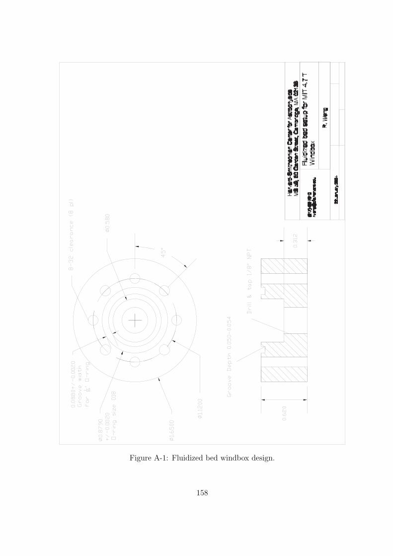
Figure A-1: Fluidized bed windbox design.
158

Figure A-2: Fluidized bed bottom diffuser plate flange design.
159

Figure A-3: Fluidized bed column mounting flange design.
160

Figure A-4: Fluidized bed gas exhaust flange design.
161

162

Appendix B
Fluidization Apparatus for a
Horizontal-Bore Magnet
163

Figure B-1: A Second Fluidization Apparatus.
164

Appendix C
Parameters Characterizing
Fluidized Beds
165

Table C.1: Fluidized-Bed Parameters
Variable DescriptionV Volume of the whole bed (V = Ve + Vb + Vs)Ve Volume of the emulsion phaseVb Volume of the bubble phaseVa Volume of the adsorption phaseVs Volume of the solid phase, Vs > Va
ε Void fraction of the whole bedεe Void fraction in emulsion (void volume divided by emulsion volume)
εmf Void fraction of the emulsion phase corresponding to minimum fluidizationψe Ratio of void space volume in emulsion to the whole bed volume, ψe = Ve
Vεe
ψb Ratio of bubble volume to the whole bed volume, ψb = Vb
V
ψa Ratio of adsorption volume to the whole bed volume, ψa = Va
V
q Volumetric gas flow rateU Superficial gas flow velocity
Umf Superficial gas flow velocity corresponding to minimum fluidizationUmb Superficial gas flow velocity corresponding to minimum bubblingue Gas flow velocity in the emulsion phaseub Bubble rising velocity
166

Appendix D
Phase-Cycling in Measurement of
the Bubble-Emulsion Exchange
In order to remove the effect of inflow gas on the measurement of the bubble-emulsion
exchange rate, we applied phase-cycling on the first 90◦ RF pulse and receiver phase,
as shown in Table D.1. The pulse sequence is shown here again for ease to read.
Two different phase sequences were used in the measurement. Their effects on
both the exchanged and inflow magnetizations are shown under the lines of the cor-
responding phase sequences, in terms of magnetization orientations. The acquired
data had the same phase after the two scans for exchanged magnetization, while 180◦
difference in the inflow magnetizations. Summation of the two group of data yielded
coherent addition of exchanged magnetization while the inflow term was cancelled.
167

2
π
RF2
π
2
π
τ τ2
π
2
π
RF2
π
2
π
1 τ2
π
ττ3
Contrast
Generation Exchange Acqusition
Figure D-1: The pulse sequence.
Table D.1: Phase-Cycling in the Sequence
Sequence π2
π π2
π2
Receiver
Phase 0 0 0 0 0Exchange Magn. +Y -Y +Z +Y +Y
Inflow Magn. N/A N/A N/A +Y +YPhase 2 0 0 0 2
Exchange Magn. -Y +Y -Z -Y +YInflow Magn. N/A N/A N/A +Y -Y
168

Appendix E
List of Rules Used in Error
Analysis
E.1 Error Propagation
Suppose y is a function of n variables labelled by xi (i = 1, · · · , n) as
y = f(x1, x2, · · · , xn). (E.1)
If we designate the standard deviations in xi values by σi and assume xi’s are inde-
pendent of each other, the standard deviation in y is then given by
∆y =
√√√√n∑
i=1
σ2i
( ∂f
∂xi
)2
. (E.2)
This is the representation of the error propagation.
E.2 Error Analysis in Least-Square Linear Fittings
Suppose we have two data vectors:
X = (x1, x2, · · · , xn) and Y = (y1, y2, · · · , yn), (E.3)
169

we want to fit them to a linear relationship given by
y = ax + b, (E.4)
where a and b are fitting parameters to be determined. The principle is to find a and
b that minimize the so-defined Chi-square:
χ =n∑
i=1
[yi − (axi + b)]2
σ2i
, (E.5)
where σi is the standard deviation of yi. According to Bevington [53], we have the
following fitting results
a = ∆[ n∑
i=1
x2i
σ2i
n∑i=1
yi
σ2i
−n∑
i=1
xi
σ2i
n∑i=1
xiyi
σ2i
]and
b = ∆[ n∑
i=1
1
σ2i
n∑i=1
xiyi
σ2i
−n∑
i=1
xi
σ2i
n∑i=1
yi
σ2i
], (E.6)
where
∆ =n∑
i=1
1
σ2i
n∑i=1
x2i
σ2i
−( n∑
i=1
xi
σ2i
)2
. (E.7)
The standard deviation of the fitting results a and b are
σa =1
∆
n∑i=1
x2i
σ2i
and
σb =1
∆
n∑i=1
1
σ2i
. (E.8)
The goodness of the linear fitting is evaluated by the correlation coefficient defined
by
R2 =
[∑ni=1(xi − x)(yi − y)
]2
∑ni=1(xi − x)2
∑ni=1(yi − y)2
. (E.9)
170

When the value of R2 is larger than 0.9, a linear relationship is considered to exist
between the two vectors.
If the data are to be fitted to any function, instead of a line, the function needs
to be reorganized into linear dependence so that the above formulations can be used.
These formula have been used in analyzing the experimental results in this thesis.
171

172

Bibliography
[1] D. Kunii. Fluidization Engineering. Butterworth-Heinemann, 1991.
[2] R. Jackson. The Dynamics of Fluidized Particles. Cambridge University Press,
2000.
[3] A. Kastler. Quelques questions concernant la production optique du ingalit
du population des niveaux de qualification spatiale des atomes. Application a
l’exprience de Stern et Gerlach et la resonance magnetique. J. Phys. Radium,
11, 1950.
[4] S. Suzuki, T. Akahori, N. Miyazawa, M. Numata, T. Okubo, and J. P. But-
ler. Alveolar surface area-to-lung volume ratio in oleic acid-induced pulmonary
edema. J. Appl. Physiol, 80, 1996.
[5] A. Seidel, F. Rittner, and B. Boddenberg. 129Xe NMR Chemical Shifts and
Linewidths of Xenon in Zeolites ZnY. J. chem. Soc. Faraday Trans, 92(493),
1996.
[6] K. Sperling-Ischinsky and W.S. Veeman. 129Xe-NMR of Carbon Black Filled
Elastomers. J. Braz. Chem. Soc, 10(4), 1999.
[7] K W Miller, N V Reo, A J Schoot Uiterkamp, D P Stengle, T R Stengle, and
K L Williamson. Xenon NMR: chemical shifts of a general anesthetic in common
solvents, proteins, and membranes. Proc. Natl. Acad. Sci, 78(8), 1981.
173

[8] N. Kato, T. Ueda, H. Omi, K. Miyakubo, and Taro Eguchi. Characteriza-
tion of adsorbed xenon in Zeolite-A, X, and Y by high-pressure 129Xe NMR
spectroscopy. Phys. Chem. Chem. Phys, 6(23), 2004.
[9] D. J. Griffiths. Introduction to Electrodynamics. Prentice Hall, Inc, 1989.
[10] C. P. Slichter. Principles of Magnetic Resonance. Harper & Row, 1963.
[11] F. Bloch. Nuclear Induction. Phys. Rev, 70, 1946.
[12] E. L. Hahn. Nuclear Induction Due to Free Larmor Precession. Phys. Rev, 77,
1950.
[13] A. Abragam. Principles of Nuclear Magnetism. Oxford University Press, 1961.
[14] A. Bifone, Y.-Q. Song, R. Seydoux, R. E. Taylor, B. M. Goodson, T. Pietrass,
T. F. Budinger, G. Navon, and A. Pines. NMR of laser-polarized xenon in
human blood. Proc Natl Acad Sci U S A, 93(23), 1996.
[15] R. W. Mair, C.-H. Tseng, D. G. Cory G. P. Wong, and R. L. Walsworth.
Magnetic Resonance Imaging of Convection in Laser-Polarized Xenon. Phys.
Rev. E, 61, 2000.
[16] B. Audoly, P. N. Sen, S. Ryu, and Y. Q. Song. Correlation functions for inho-
mogeneous magnetic field in random media with application to a dense random
pack of spheres. J. Magn. Reson, 164(1), 2003.
[17] A. Fick. Ann. Physik, Leipzig, 170, 1855.
[18] P. T. Callaghan. Principles of Nuclear Magnetic Resonance Microscopy. Oxford
University Press, 1995.
[19] E. O. Stejskal and J. E. Tanner. Spin Diffusion Measurements: Spin Echoes in
the Presence of a Time-Dependent Field Gradient. J. Chem. Phys., 42, 1965.
[20] G. P. Wong, C.-H. Tseng, V. R. Pomeroy, R. W. Mair, D. P. Hinton, D. Hoff-
mann, R. E. Stoner, F. W. Hersman, D. G. Cory, and R. L. Walsworth. A
174

system for low field imaging of laser-polarized noble gas. Journal of Magnetic
Resonance, 141, 1998.
[21] R. W. Mair, C.-H. Tseng, G. P. Wong, D. G. Cory, and R. L. Walsworth.
Magnetic Resonance Imaging of Convection in Laser-Polarized Xenon. Phys.
Rev. E, 61, 2000.
[22] K. W. Miller, N. V. Reo, A. J. Uiterkamp, D. P. Stengle, T. R. Stengle, ,
and K. L. Williamson. Xenon NMR: Chemical Shifts of a General Anesthetic
in Common Solvents, Proteins, and Membranes. Proc Natl Acad Sci U S A,
78(8), 1981.
[23] P. T. Callaghan, A. Coy, D. MacGowan, K. J. Packer, and F. O. Zelya.
Diffraction-Like Effects in NMR Diffusion Studies of Fluids in Porous Solids.
Nature, 351, 1991.
[24] P. P. Mitra, P. N. Sen, and L. M. Schwartz. Short-Time Behavior of the Diffusion
Coefficient as a Geometrical Probe of Porous Media. Phys. Rev. B, 47, 1993.
[25] R. W. Mair and R. L. Walsworth. Novel MRI Applications of Laser-Polarized
Noble Gases. Appl. Magn. Reson, 22, 2002.
[26] W. Happer. Optical Pumping. Rev. Mod. Phys, 44(2), 1972.
[27] S. Aplett, A. B. Baranga, and C. J. Erickson et al. Theory of spin-exchange
optical pumping of 3He and 129Xe. Phys. Rev. A, 58(2), 1998.
[28] A. Oros and N. Shah. Hyperpolarized xenon in NMR and MRI. Phys. Med.
Biol, 49, 2004.
[29] M. S. Rosen. Laser Polarized Xe-129 Magnetic Resonance Spectroscopy and
Imaging; the Development of a Method for in vivo Perfusion Measurement.
Thesis, 2001.
175

[30] M. A. Bouchiat, J. Brossel, and L. C. Pottier. Evidence for Rb-rare-gas
molecules from the relaxation of polarized Rb atoms in a rare gas. Experimental
Results. J. Chem. Phys, 56, 1972.
[31] G. D. Cates, R. J. Fitzgerald, and A. S. Barton et al. Rb-129Xe spin-exchange
rates due to binary and three-body collisions at high Xe pressures. Phys. Rev.
A, 45, 1992.
[32] G. P. Wong. Nuclear Magnetic Resonance Experiments Using Laser-Polarized
Noble Gas. Thesis, 2001.
[33] A. G. Richter, C. J. Yu, A. Datta, J. Kmetko, and P. Dutta. In situ and inter-
rupted growth studies of the self-assembly of octadecyltrichlorosilane monlayers.
Phys. Rev. E, 61, 2000.
[34] B. Driehuys, G. D. Cates, and W. Happer. Surface Relaxation Mechanisms of
Laser-Polarized 129Xe. Phys. Rev. Lett., 74:4943–4946, 1995.
[35] N. Bloembergen, E. M. Purcell, and R. V. Pound. Relaxation effects in nuclear
magnetic resonance absorption. Phys. Rev, 73, 1948.
[36] J. Bear. Dynamics of Fluids in Porous Media. Elsevier Inc., New York, 1972.
[37] S. Whitaker. A Theoretical Derivation of Darcy’s Law. Transport Porous Med.,
1, 1986.
[38] R. Meyer and F. F. Krause. Experimental Evidence for Permeability Minima
at Low-Velocity Gas Flow Through Naturally Formed Porous Media. J. Porous
Med., 1, 1998.
[39] M. D. Hrlimann, K. G. Helmer, L. L. Latour, and C. H. Sotak. Restricted Dif-
fusion in Sedimentary Rocks. Determination of Surface-Area-to-Volume Ratio
and Surface Relaxivity. J. Magn. Reson. Series A, 111, 1994.
176
[40] D. B. Stephens, K.-C. Hsu, M. A. Prieksat, M. D. Ankeny, N. Blandford, T. L.
Roth, J. A. Kelsey, and J. R. Whitworth. A Comparison of Estimated and
Calculated Effective Porosity. Hydrogeol. J, 6, 1998.
[41] P. Z. Wong. Dynamics of Fluids in Porous Media. Academic Press, London,
1999.
[42] M. Sahimi. Flow phenomena in rocks: from continuum models to fractals,
percolation, cellular automata, and simulated annealing. Rev. Mod. Phys, 65,
1993.
[43] D. P. Ours, D. I. Siegel, and P. H. Glaser. Chemical dilation and the dual
porosity of humidified peat bog. J. Hydrol, 196, 1997.
[44] T. G. Walker and W. Happer. Spin-exchange optical pumping of noble-gas
nuclei. Rev. Mod. Phys, 69:629–642, 1997.
[45] J. P. Butler, R. W. Mair, D. Hoffmann, M. I. Hrovat, R. A. Rogers, G. P. Top-
ulos, R. L. Walsworth, and S. Patz. Measuring Surface-Area-to-Volume Ratios
in Soft Porous Materials using Laser-Polarized Xenon Interphase Exchange Nu-
clear Magnetic Resonance. Phys. Rev. E, 14, 2002.
[46] Y.-Q. Song. Determining Pore Sizes Using an Internal Magnetic Field. J. Magn.
Reson, 143, 2000.
[47] M. S. Rosen, T. E. Chupp, K. P. Coulter, R. C. Welsh, and S. D. Swanson. Po-
larized Xe-129 optical pumping/spin exchange and delivery system for magnetic
resonance spectroscopy and imaging studies. Rev. Sci. Instrum, 70, 1999.
[48] H. Y. Carr and E. M. Purcell. Effects of Diffusion on Free Precession in Nuclear
Magnetic Resonance Experiments. Phys. Rev, 94, 1954.
[49] H. Huang, K. Wang, D. M. Bodily, and V. J. Hucka. Density Measurements of
Argonne Premium Coal Samples. Energ. Fuel, 9, 1996.
177

[50] M. Bencsik and C. Ramanathan. Method for measuring local hydraulic perme-
ability using magnetic resonance imaging. Phys. Rev. E, 63(065302), 2001.
[51] R. E. Jacob, S.W. Morgan, and B. Saam. Wall Relaxation of 3He in Spin-
Exchange Cells. Phys. Rev. E, 87(143004), 2001.
[52] R. W. Fox and A. T. McDonald. Introduction to Fluid Mechanics. John Wiley
& Sons Inc., New York, 1998.
[53] P. R. Bevington and D. K. Robinson. Data Reduction and Error Analysis for
The Physical Sciences. McGraw-Hill Science, 1991.
[54] C.-H. Tseng, G. P. Wong, V. R. Pomeroy, R. W. Mair, D. P. Hinton, D. Hoff-
mann, R. E. Stoner, F. W. Hersman, D. G. Cory, and R. L. Walsworth. Low-
Field MRI of Laser Polarized Noble Gas. Phys. Rev. Lett, 81, 1998.
[55] M. J. Nicholl, H. Rajaram, and R. J. Glass. Factors controlling satiated relative
permeability in a partially-saturated horizontal fracture. Geophys. Res. Lett,
27, 2000.
[56] M. Jamiolahmady, A. Danesh, D. H. Tehrani, and D. B. Duncan. Positive effect
of flow velocity on gas-condensate relative permeability: Network modeling and
comparison with experimental results. Transport Porous Med, 52, 2003.
[57] R. M. Nedderman. Statics and Kinematics of Granular Materials. Cambridge
University Press, 1992.
[58] B. J. Ennis, J. Green, and R. Davies. The legacy of neglect in the U.S. Chem.
Eng. Prog, 90:32–43, 1994.
[59] J. Z. Xue, E. Herbolzheimer, M. A. Rutgers, W. B. Russel, and P. M. Chaikin.
Diffusion, Dispersion, and Settling of Hard Spheres. Phys. Rev. Lett, 69(11),
1992.
[60] K. Rietema. The effect of interparticle forces on the expansion of a homogeneous
gas-fluidised bed. Chem. Eng. Sci, 28, 1973.
178

[61] S. C. Tsinontides and R. Jackson. The mechanics of gas fluidized beds with an
interval of stable fluidization. J. Fluid Mech, 255, 1993.
[62] N. Menon and D. J. Durian. Particle Motions in a Gas-Fluidized Bed of Sand.
Phys. Rev. Lett, 79(18), 1997.
[63] J. M. Valverde, A. Castellanos, and M. A. Quintanilla. Self-Diffusion in a Gas-
Fluidized Bed of Fine Powder. Phys. Rev. Lett, 86(14), 2001.
[64] P. U. Foscolo and L. G. Gibilaro. A fully predictive criterion for the transition
between particulate and aggregate fluidization. Chem. Eng. Sci, 39, 1984.
[65] D. Geldart. Gas Fluidization Technology. John Wiley & Sons Ltd, 1986.
[66] D. Geldart. Types of gas fluidization. Powder Technol, 7, 1978.
[67] P.C. Carman. Fluid flow through a granular bed. Trans. Inst. Chem. Eng, 15,
1937.
[68] C. Y. Wen and Y. H. Yu. A generalized method for predicting the minimum
fluidization velocity. AIChE J, 21, 1966.
[69] D. Geldart and A. R. Abrahamsen. Powder Technol, 19, 1978.
[70] R. M. Davies and G. I. Taylor. The mechanics of large bubbles rising through
extended liquids and through liquids in tubes. Proc. Roy. Soc. London Ser. A,
200, 1950.
[71] J. F. Davidson and D. Harrison. Fluidized Particles. Cambridge University
Press, 1963.
[72] J. F. Davidson, D. Harrison, and J. R. F. Guedes de Carvalho. On the Liquidlike
Behavior of Fluidized Beds. Ann. Rev. Fluid Mech, 9, 1977.
[73] R. R. Cranfield and D. Geldart. Large particle fluidisation. Chem. Eng. Sci,
29(4), 1974.
179

[74] A. Bifone, T. Pietrass, J. Kritzenberger, and A. Pines. Surface Study of Sup-
ported Metal Particles by 129Xe NMR. Phys. Rev. Lett, 74(16), 1995.
[75] A. Gedeon, J. L. Bonardet, T. Ito, and J. Fraissard. Application of
129Xe NMR to the Study of Ni2+ Y Zeolites. J. Phys. Chem, 93, 1989.
[76] I. L. Moudrakovski, A. Nossov, S. Lang, S. R. Breeze, C. I. Ratcliffe, B. Simard,
G. Santyr, and J. A. Ripmeester. Continuous Flow NMR with Hyperpolarized
Xenon for the Characterization of Materials and Processes. Chem. of Materials,
12(5), 2000.
[77] M. Mansfeld and W. S. Veeman. 129Xe Nuclear Magnetic Resonance of Al2O3
fibers. Microporous Materials, 3, 1994.
[78] R. Higbie. The rate of adsorption of a pure gas into a still liquid during short
periods of exposure. Trans. Am. Inst. Chem. Eng, 31, 1935.
[79] L. Davies and J. F. Richardson. Gas interchange between bubbles and the
continuous phase in a fluidized bed. Trans. Inst. Chem. Eng, 44, 1966.
[80] G. K. Stephens, R. J. Sinclair, and O. E. Potter. Gas exchange between bubbles
and dense phase in a fluidised bed. Powder Technol, 1, 1967.
[81] T. Chiba and H. Kobayashi. Gas exchange between the bubble and emulsion
phases in gas-solid fluidized beds. Chem. Eng. Sci, 25, 1970.
[82] J. R. Grace. Recent Advances in the Engineering Analysis of Chemcially Re-
acting Systems. Wiley, New Delhi, 1984.
[83] D. J. Patil, M. S. Annaland, and J.A.M. Kuipers. Gas Dispersion and Bubble-
to-Emulsion Phase Mass Exchange in a Gas-Solid Bubbling Fluidized Bed: A
Computational and Experimental Study. Int. J. of Chem. Reactor Eng, 1(44),
2003.
[84] C. Chavarie and J. R. Grace. Interphase mass transfer in a gas-fluidized bed.
Chem. Eng. Sci, 31, 1975.
180

[85] S. P. Sit and J. R. Grace. Interphase mass transfer in an aggregative fluidized
bed. Chem. Eng. Sci, 33, 1977.
[86] W. E. Resnick and R. R. White. Mass transfer in systems of gas and fluidized
solids. Chem. Eng. Prog, 45, 1949.
[87] K. N. Kettenring, E. L. Manderfield, and J. M. Smith. Chem. Eng. Prog, 46,
1950.
[88] J. C. Chu, J. Kalil, and W. A. Wetteroth. Mass transfer in a fluidized bed.
Chem. Eng. Prog, 49, 1953.
[89] T. Kai, T. Imamura, and T. Takahashi. Hydrodynamic influences on mass
transfer between bubble and emulsion phases in a fine particle fluidized bed.
Powder Technol, 83, 1994.
[90] P. W. Percival and J. S. Hyde. Saturation-recovery measurements of the spin-
lattice relaxation times of some nitroxides in solution. J. Magn. Reson, 23,
1976.
[91] R. Savelsberg, D. E. Demco, B. Blumich, and S. Stapf. Particle motion in gas-
fluidized granular systems by pulsed-field gradient nuclear magnetic resonance.
Phys. Rev. E, 65(020301), 2002.
[92] E. E. Ehrichs, H. M. Jaeger, G. S. Karczmar, Y. V. Kuperman J. B. Knight, and
S. R. Nagel. Granular Convection Observed by Magnetic Resonance Imaging.
Science, 267, 1995.
[93] R. W. Mair, M. S. Rosen, R. Wang, D. G. Cory, and R. L. Walsworth. Diffusion
NMR Methods Applied to Xenon Gas for Materials Study. Magn. Reson. Chem,
40, 2002.
[94] R. W. Mair, R. Wang, M.S. Rosen, D. Candela, D.G. Cory, and R.L. Walsworth.
Applications of Controlled-Flow Laser-Polarized Xenon Gas to Porous and
Granular Media Study. Magn. Reson. Imag, 21, 2003.
181

[95] D. W. Alderman and D. M. Grant. An efficient decoupler coil design which
reducesheating in conductive samples in superconducting spectrometers. J.
Magn. Reson, 36, 1979.
[96] R. Ojha, N. Menon, and D. J. Durian. Hysteresis and packing in gas-fluidized
beds. Phys. Rev. E, 62(3), 2000.
[97] S. C. Saxena and G. J. Vogel. The measurement of incipient fluidization ve-
locities in a bed of coarse dolomite at temperature and pressure. Trans. Inst.
Chem. Eng, 55(3), 1977.
[98] D. C. Chitester, R. M. Kornosky, L. Fan, and J. P. Danko. Characteristics of
fluidization at high pressure. Chem. Eng. Sci, 39(2), 1984.
[99] X. Yang, C. Huan, D. Candela, R. W. Mair, and R. L. Walsworth. Measure-
ments of Grain Motion in a Dense, Three Dimensional Granular Fluid. Phys.
Rev. Lett, 88(044301), 2000.
[100] J. C. Orcutt, J. F. Davidson, and R. L. Pigford. Reaction time distributions in
fluidized catalytic reactors. Chem. Eng. Prog. Sym. Ser, 58(387), 1962.
182