study of effective distances for interpolation schemes in

HAL Id: hal-00465570https://hal-mines-paristech.archives-ouvertes.fr/hal-00465570

Submitted on 19 Mar 2010

HAL is a multi-disciplinary open accessarchive for the deposit and dissemination of sci-entific research documents, whether they are pub-lished or not. The documents may come fromteaching and research institutions in France orabroad, or from public or private research centers.

L’archive ouverte pluridisciplinaire HAL, estdestinée au dépôt et à la diffusion de documentsscientifiques de niveau recherche, publiés ou non,émanant des établissements d’enseignement et derecherche français ou étrangers, des laboratoirespublics ou privés.

Study of effective distances for interpolation schemes inmeteorology

Mireille Lefèvre, Jan Remund, Michel Albuisson, Lucien Wald

To cite this version:Mireille Lefèvre, Jan Remund, Michel Albuisson, Lucien Wald. Study of effective distances for inter-polation schemes in meteorology. European Geophysical Society, 27th General Assembly, Apr 2002,Nice, France. pp.A-03429. �hal-00465570�

https://hal-mines-paristech.archives-ouvertes.fr/hal-00465570

https://hal.archives-ouvertes.fr

Presented to the XXVII Annual Assembly, European Geophysical Society, Nice, April 2002, Geophysical Research Abstracts, vol. 4, April 2002, EGS02-A-03429.

STUDY OF EFFECTIVE DISTANCES FOR INTERPOLATION SCHEMES IN

METEOROLOGY

Mireille LEFEVRE (1), Jan REMUND (2), Michel ALBUISSON (1), Lucien WALD (1)

(1) Ecole des Mines de Paris / Armines, BP 207, 06904 Sophia Antipolis cedex, France

(2) Meteotest, Fabrikstrasse 14, 3012 Bern, Switzerland

Corresponding author: Lucien WALD.

[email protected]. Tel: 33 493957449. Fax 33 493957535

Copyright Ecole des Mines de Paris - Armines - Meteotest 1


ABSTRACT:

This work explores the possibility of integrating the geographical elements such as orography

and presence of water bodies as well as the latitudinal effects into an effective distance when

interpolating meteorological fields. This effective distance may then be used in any

interpolation methods instead of the standard geodetic distance. Several hundreds of sites are

used in Europe to assess the benefits of several effective distances. The meteorological

parameters under concern are ten-years averages of monthly means of daily sum of horizontal

global irradiation, daily sum of sunshine duration, daily extremes of air temperature,

atmospheric pressure and water vapor pressure, and of monthly sums of precipitation. This

work demonstrates that taking into account the latitudinal effects in the distance increases the

accuracy in interpolation. Such effects have been seldom mentioned in previous publications.

The orographic effects may be partly corrected by adding the weighted difference in elevation

to the geodetic distance. The following effective distance between the point P and each of the

measuring sites Xi for all parameters, is found to give better results than the others:

deff2 = fNS

2 (dgeo2 + foro

2 δh2)

with fNS = 1 + 0.3 ΦP -ΦX [1+ (sinΦP + sinΦX) / 2], where dgeo is the geodetic distance in

km, latitudes ΦP and ΦX are expressed in degrees, δh is the difference in elevation between P

and Xi (expressed in km) and foro is set to 500.

Keywords: interpolation, distance, latitude, meteorology, irradiation



INTRODUCTION

In meteorology, as well as in other geophysical sciences, Earth surface processes are mostly

known by the means of networks of ground-based instruments though increasing use is made

of satellite observations. Each network is scarce and interpolation methods are necessary to

assess the value V(P) of the parameter under concern for any geographical point P located

between the sites of measurements Xi.

There is a wealth of publications dealing with the interpolation of meteorological fields. This

work does not propose a new method but focuses on the definition of the distance between

sites, a distance that is used in all methods. An important aspect of our work is the ability to

perform a fast interpolation using an unknown number of measuring sites, especially in the

framework of the Web service SoDa, which exploits a smart network of distributed resources

to deliver information relating to the solar radiation (Rigollier et al. 2000). Several resources

necessitate estimates of meteorological fields at any point in the world (SoDa 2001). These

estimates should be provided by a fast interpolation technique.

The problem of interpolation may be seen as an adjustment mathematical problem, that is

what is the hyper-surface that fits best the observed values V(Xi)? (Picinbono 1986). This

surface is usually defined in an analytical form but piecewise polynomials, e.g., B-splines are

often very appropriate (Hou, Andrews 1978). Once the parameters of the model known by

adjustment over the observed values, it provides a value for any geographical point P for the

area under concern. Least-square fitting of surfaces of polynomial type on a global or local

scale, thin plate method or Hsieh-Clough-Tocher method, are examples of such methods

(Hutchinson et al. 1984; Hulme et al. 1995). One of their advantages is the degree of

continuity of the derivatives of the estimated field.



A more conventional approach consists in estimating the meteorological parameter at the

single geographical point P using the nearest sites where measurements are made. The

estimated value is a combination of the measurements V(Xi) weighted by a function of the

distance di between the point P and each of the measuring sites Xi. The shorter the distance,

the larger the influence of the site and the larger the weight of the site in the combination. The

estimated value V(P) is expressed as:

V(P) = (1)

where V(Xi) is the value measured by the ith site among the nearest N measuring sites and wi is

the weight for this site, with = 1.

In such a linear interpolation, there is no bias, that is that the estimated field V* takes the

measured values V(Xi) at the geographical points Xi located over the measuring sites. This

may not be the case for the fields resulting from a method based upon adjustment

mechanisms. However, the first derivative of the field resulting from a linear interpolation is

not continuous. Popular methods like kriging, objective analysis, and inverse squared distance

are examples of linear interpolation methods (Journel, Huijbregts 1978; Thiébaux, Pedder

1987). In the inverse squared distance method, also called gravity method, the weights wi are

given by

wi = / (2)

where di, dj are respectively the distances from respectively the site Xi and the sites Xj to the

geographical point P:

ii PXd = and di, dj ≠ 0 (3)

Different methods use different weights. Some methods make use of the estimated spatial

structure of the field itself to compute the weights. This structure is expressed by e.g. the

variogram or the correlation function.



Whatever the method, of adjustment type or linear type, a distance between the sites and the

geographical point P is computed. It is usually the geodetic distance or the Euclidean distance

if the data are located on a grid whose cells are regularly spaced. Given two sites P and X of

geographical co-ordinates (ΦP, λP) and (ΦX, λX), where Φ and λ stand for latitude and

longitude, the geodetic distance dgeo between P and X is:

dgeo = R Θ (4)

where

cos Θ = sin ΦP sin ΦX + cos ΦP cos ΦX cos(λP - λX) (5)

where Θ is expressed in radians and (λP - λX) is the difference in longitude. The geodetic

distance is the distance at the surface of the Earth considered as a sphere of radius R (R= 6371

km). It is also called the horizontal distance. Here, the latitude is counted positive from the

equatorial plane northwards and negative southwards. The longitude is counted positive

eastwards from the Greenwich meridian and negative westwards.

TAKING INTO ACCOUNT NATURAL PROCESSES

The spatial structure of a meteorological field is a function, usually complex, of several

natural processes. Among others are the latitudinal effects and the orography. They should be

taken into account for a better estimate of the field. Some methods, like the co-kriging, offer

the possibility to take into account the cross-variation or the cross-structure of the

meteorological parameter under concern and of another parameter. This additional parameter

should be positively correlated to the first one and sampled for a larger number of locations.

The range of values of the second parameter taken by the measuring sites should be large, too.

Finally, the set of values should represent the field under concern. This is not often the case,

as shown by the example of France in the construction of the European Solar Radiation Atlas



(ESRA, 2000). In this case, forty-four stations were used that measure global irradiation,

sunshine duration, air temperature and pressure at ground level, precipitation and water vapor.

Out of these 44 sites, only 12 have elevations greater than 200 m (27 % of the total). Out of

these 12, three have elevation greater than 400 m (7 %) and three have elevation between 300

and 400 m. The range of elevation described by these sites is too narrow to establish an

accurate description of the effects of the orography: approximately 40 % of the French

territory exhibit elevation greater than 200 m, and more than 15 % has elevation higher than

500 m. The data set does not reproduce the distribution of the elevation values.

The use of detailed additional information may improve the results of the interpolation at the

expenses of computational complexity. Co-kriging is often used in such cases, though other

techniques prove as efficient (Beyer et al. 1997; Hudson, Wackernagel 1994; Lo 1989;

Zelenka et al. 1992). In the construction of the European Solar Radiation Atlas (ESRA 2000),

a segmentation of Europe was performed by the means of clustering analysis before

proceeding to interpolation using a gravity method. In a similar way, Supit (1994) proposes to

combine interpolated values of the Angström coefficients, representative sunshine duration

for the area under concern and a regression model to estimate the solar irradiation. In their so-

called climatologically aided interpolation method, Willmott and Robeson (1995) make a

combined use of air temperature climatology and interpolated temperature deviations at

measuring sites. Typical circulation patterns may be used to guide the interpolation (Courault,

Monestiez 1999). Kunz, Remund (1995) used detailed models describing local relationships

between orography and meteorological fields for Switzerland, a country with a very dense

network of measuring stations. Some methods make use of multiple linear regression analysis

of data from a set of nearby measuring sites to locally model changes in meteorological fields.

The value at the point P is predicted from these sites using the regression curve, each site Xi



being in addition inverse-weighted by its distance to P (Anonymous 1995; Jones, Thornton

1999; Nalder, Wein 1998; Price et al. 2000; � en, � ahin 2001; Van der Goot 1999; Van der

Voet et al. 1994).

Beside these efforts, other authors tried to integrate the natural processes into the definition of

an effective distance. This process-based distance is then used in any interpolation method,

instead of the geodetic distance. This is the approach selected for this work. Compared to

other techniques, the use of an effective distance permits to develop fast interpolation

methods that can be launched within a Web service.

THE EFFECTIVE DISTANCE

Beyer et al. (1997), MeteoNorm (2000) or Zelenka et al. (1992) used an effective distance:

deff = (6)

where dgeo is the geodetic distance between the measuring site X and the current location P

and δh is the difference in elevation of both locations. The geodetic distance and the elevation

should be expressed in the same units, e.g. in km. The parameter f controls the equivalence

between horizontal and vertical distances. f is set to 100 by Zelenka et al. and to 300 by Beyer

et al. The latter stress that the results are only weakly dependent upon f, for most of the

elevation differences encountered in their work. This effective distance was then used in co-

kriging or inverse squared distance interpolation.

Anonymous (1995) and Van der Voet et al. (1994) studied an effective distance taking into

account the absolute difference in elevation of both locations, the possible presence of a

climatic barrier between the site X and the point P and the distance to the coastline.

The present work explores various ways to take into account the orography, the effect of the

latitude and the presence of the large water bodies. This exploration is possible because all



necessary information is now available for the whole Earth in a digital form and with a

sufficient accuracy. When launching the present study, it was expected that a better

representation of the orographic features and profiles would lead to a better accuracy in

interpolation.

The effective distance deff is based on the geodetic distance that is effectively increased to take

into account some processes:

deff2 = flat

2 fNS2 (dgeo

2 + foro2 doro

2 + fsea2 dsea

2) (7)

where flat and fNS are taking into account the latitudinal effects, (foro doro) is the additional

distance taking into account the orography and (fsea dsea) that induced by large water bodies.

Latitudinal effects

The meteorological fields have well-marked distributions along the latitudes. They are

anisotropic: the fields tend to be homogeneous along the latitude with strong North-South

gradients (see e.g., Anthes 1997; Atlas of hydrometeorological data 1991; ESRA 2000).

The meteorological phenomena are preferentially moving along the latitudes. Their size and

lifetime are related to each other and the relationship is independent from the latitude at first

order. We studied the possible normalization of the geodetic distance by the perimeter of the

latitude of the site P. Actually, we found out that this transformation has a negligible impact

on the results. Price et al. (2000) reported a similar result. Accordingly, the factor flat is set to

1.

Another factor fNS is introduced to model the anisotropy of the fields and to penalize the

North-South distances:

fNS = 1 + aNS ΦP -ΦX [1+ (sinΦP + sinΦX) / 2] (8)

where aNS is an arbitrary parameter.



Orography

In the Equation [6], the orographic effects are represented by a difference in elevation. This

does not reproduce the case of an orographic barrier separating two sites P and X of equal

elevation. It is proposed to use instead the profile of elevation. Given an elevation profile

extracted from a gridded digital elevation model (DEM), and approximating a grid cell by its

center, the distance di at the ground surface between two cells i and i+1 of elevation hi and

hi+1 is:

di2 = dgeo

2 + (hi+1 - hi)2 (9)

We thus define the orographic distance as:

doro2(P, Xi) = (10)

where N is the number of cells comprised between P and Xi, along the shortest geodetic

distance. The distance doro penalizes elevation profiles [P, Xi,] offering large elevation

gradients. The digital elevation model used is the model TerrainBase (1995). The size of the

grid cell is 5' of arc angle (approximately 10 km at mid-latitude) and the elevation step is 1 m.

The algorithm of Bresenham (1965) was used for computing orographic profiles. It is fast and

works in integer values.

The meteorological parameters strongly depend upon the elevation. We enforce the

orographic distance doro by multiplying it by the parameter foro. It controls the equivalence

between the horizontal and vertical distances. Setting foro to 500 means that a difference in

elevation of 100 m is equivalent to a geodetic distance of 50 km.

Other orographic distances are computed for comparison with doro. We define the elevation

difference distance: foro δh, where δh is the difference in elevation between P and Xi, like in

Equation 6, and the elevation maximum difference distance: foro ∆Η, where ∆Η is the



maximum difference in height that can be found in the orographic profile between P and Xi: it

is the absolute value of the difference between the highest point and the lowest one.

Water bodies effect

Large water bodies separating sites may create climatological barriers. The geodetic distance

over such water bodies between P and Xi is called dsea. Using TerrainBase in an appropriate

manner, one may represent large water bodies and thus compute dsea using the same cell size

than for orography. Adding a quantity equal to fsea dsea, where fsea is determined in an empirical

way, penalizes the geodetic distance. The influence of the component (fsea2 dsea

2) was assessed

by using a selected number of sites of similar elevations, which are separated by large water

bodies (e.g., sites in Azores Islands, Eire and Spain). Actually, we found that the influence of

the water bodies component is negligible. Varying fsea from 0 to 10 does not lead to a

noticeable change in accuracy. Accordingly, this component is disregarded.

DATABASE AND TESTS

The various components of the effective distance were assessed for an area encompassing

Europe, ranging from 30° West to 70° East and from 25° to 75° North. Ten-year averages of

monthly means of several parameters are available in the CD-ROM of the ESRA (2000):

• daily sums of horizontal global irradiation for 586 sites,

• daily sum of sunshine duration for 556 sites,

• daily extreme of air temperature for 435 sites,

• monthly sum of precipitation for 435 sites,

• atmospheric pressure for 266 sites,

• water vapor pressure for 274 sites.

The daily irradiations and the daily sums of sunshine duration were converted into

respectively daily clearness indices KT and relative sunshine durations S/S0.



For each parameter, each site is in turn assumed to be unknown and the value of the parameter

is assessed by interpolation technique using the other sites for each month. The estimates are

compared to the measured values and the discrepancies are computed. The set of

discrepancies for all sites is then analyzed as a function of month, latitude, site, longitude and

elevation. Two quantities are computed to synthesize the discrepancies: the bias and the root

mean square.

Two interpolation techniques are used: the gravity method and the nearest-neighbor method.

Having two methods permit to compare the results and the conclusions reached for each of

them regarding the distances. Several distances are tested and compared. For each distance

and if relevant, empirical parameters were adjusted in order to decrease the errors in

interpolation:

• distance D1 (geodetic): D1 = dgeo

• distance D2 (equation [6]): D22 = (dgeo2 + f2 δh2). Elevations are in km. According to MeteoNorm

(2000), the quantity f is set to 300 for radiation parameters, 100 for temperature, 200 for precipitation and 100 for air pressure and water vapor pressure.

• distance D3: D3 = fNS dgeo, with fNS = 1 + aNS ΦP -ΦX [1+ (sinΦP + sinΦX) / 2]. Latitudes are expressed in degrees. The value of aNS leading to the smallest error in interpolated value was found to be 0.3. Nevertheless, the range of values [0.2, 0.4] gives similar errors.

• distance D4: D42 = fNS2 (dgeo

2 + foro2 doro

2)


2 + foro2 δh2)


2 + foro2 ∆H2)

For distances D4, D5 and D6, the quantity foro was set to 500, with elevation in km. The

influence of the exact value of foro on the error is negligible, provided foro is approximately in

the range [100, 1000]. This value is the same for all meteorological parameters.

RESULTS

The results show the large influence of the parameter fNS on the error in interpolation.

Compared to the distance D1 (geodetic) and D2, the distance D3 provides better results. The



incorporation of the latitudinal effects in the effective distance is the major contributor to the

increase in accuracy with respect to the standard distances.

The accuracy is further increased by the inclusion of the orographic effects (distances D4, D5

and D6). We were disappointed by the results obtained by the distance D4, taking into

account the profile of elevation between the point P and the site Xi. An improvement of

accuracy was expected, which was not evidenced at all. Better results are attained by simpler

formulae, such as the distances D5 and D6. The results attained for the distances D5 and D6

are similar, with a slight advantage to D5. This distance D5 has also a major advantage: it is

faster to compute than D6. Finally, it should be noted that the influence of the orography

correction is small compared to that of the latitudinal effects.

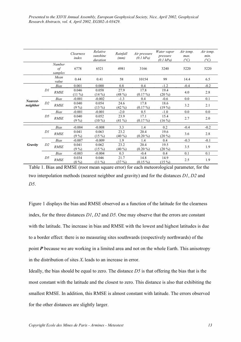
Table 1 gives the bias and RMSE (root mean square error) for each meteorological parameter,

for the two interpolation methods (nearest neighbor and gravity) and for the distances D1, D2

and D5. In all cases the smallest bias and RMSE are observed for the distance D5. Radiation

parameters are reproduced with an accuracy of approximately 10 % or better. For irradiation,

these results are similar to those reported in WMO (1981) for geodetic distances less than 400

km. Accuracy on rainfall is poor; it is well known that rainfall is a discrete field and that such

interpolation methods are not appropriate to estimate precipitation. On the contrary,

climatological means of air pressure are fairly continuous fields and these interpolation

methods give very good results. As for the air temperature, bias is small and RMSE amounts

to approximately 2 °C. When compared to the results of Hulme et al. (1995), based on a

fitting of much more stations (approximately 800) using a thin-plate technique, covering the

same area and dealing with similar types of data, our errors with distance D5 are similar for

the precipitation and larger for the sunshine duration, air temperature and water vapor

pressure.



Clearness index

Relative sunshine duration

Rainfall(mm)

Air pressure(0.1 hPa)

Water vapor pressure(0.1 hPa)

Air temp. max.(°C)

Air temp. min.(°C)

Number of

samples6778 6521 4981 3166 3240 5220 5220

Mean value 0.44 0.41 58 10154 99 14.4 6.5

Nearest-neighbor

D1Bias 0.001 0.000 0.8 0.4 -1.2 -0.4 -0.2

RMSE 0.046(11 %)

0.058(14 %)

27.9(48 %)

17.8(0.17 %)

19.4(20 %) 4.0 2.8

D2Bias -0.001 -0.002 -1.3 0.4 -0.6 0.0 0.1

RMSE 0.040(9 %)

0.054(13 %)

24.6(42 %)

17.8(0.17 %)

18.6(19 %) 3.2 2.1

D5Bias -0.001 -0.001 -2.0 0.5 -1.0 0.0 0.0

RMSE 0.040(9 %)

0.052(10 %)

23.9(41 %)

17.1(0.17 %)

15.4(16 %) 2.7 2.0

Gravity

D1Bias -0.004 -0.008 3.3 1.4 0.2 -0.4 -0.2

RMSE 0.041(9 %)

0.063(15 %)

23.2(40 %)

20.4(0.20 %)

19.6(20 %) 3.6 2.8

D2Bias -0.007 -0.009 1.9 1.4 0.4 -0.3 -0.1

RMSE 0.041(9 %)

0.062(15 %)

23.2(40 %)

20.4(0.20 %)

19.5(20 %) 3.5 1.9

D5Bias -0.003 -0.004 0.3 -0.4 0.4 0.1 0.1

RMSE 0.034(8 %)

0.046(11 %)

21.7(37 %)

14.8(0.15 %)

14.9(15 %) 2.5 1.9

Table 1. Bias and RMSE (root mean square error) for each meteorological parameter, for the

two interpolation methods (nearest neighbor and gravity) and for the distances D1, D2 and

D5.

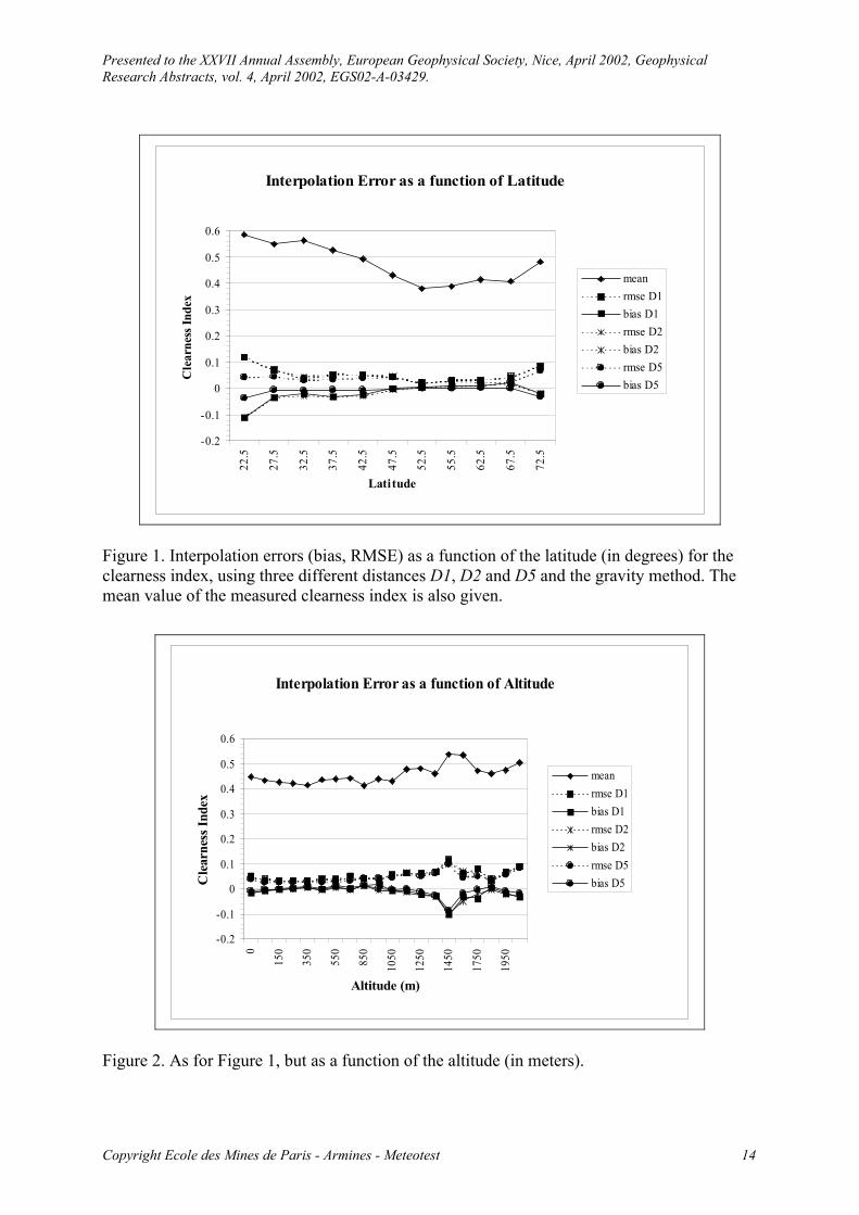
Figure 1 displays the bias and RMSE observed as a function of the latitude for the clearness

index, for the three distances D1, D2 and D5. One may observe that the errors are constant

with the latitude. The increase in bias and RMSE with the lowest and highest latitudes is due

to a border effect: there is no measuring sites southwards (respectively northwards) of the

point P because we are working in a limited area and not on the whole Earth. This anisotropy

in the distribution of sites Xi leads to an increase in error.

Ideally, the bias should be equal to zero. The distance D5 is that offering the bias that is the

most constant with the latitude and the closest to zero. This distance is also that exhibiting the

smallest RMSE. In addition, this RMSE is almost constant with latitude. The errors observed

for the other distances are slightly larger.



Interpolation Error as a function of Latitude

-0.2

-0.1

0

0.1

0.2

0.3

0.4

0.5

0.622

.5

27.5

32.5

37.5

42.5

47.5

52.5

55.5

62.5

67.5

72.5

Latitude

Cle

arne

ss In

dex

meanrmse D1bias D1rmse D2bias D2rmse D5bias D5

Figure 1. Interpolation errors (bias, RMSE) as a function of the latitude (in degrees) for the clearness index, using three different distances D1, D2 and D5 and the gravity method. The mean value of the measured clearness index is also given.

Interpolation Error as a function of Altitude

-0.2

-0.1

0

0.1

0.2

0.3

0.4

0.5

0.6

0

150

350

550

850

1050

1250

1450

1750

1950

Altitude (m)

Cle

arne

ss In

dex

meanrmse D1bias D1rmse D2bias D2rmse D5bias D5

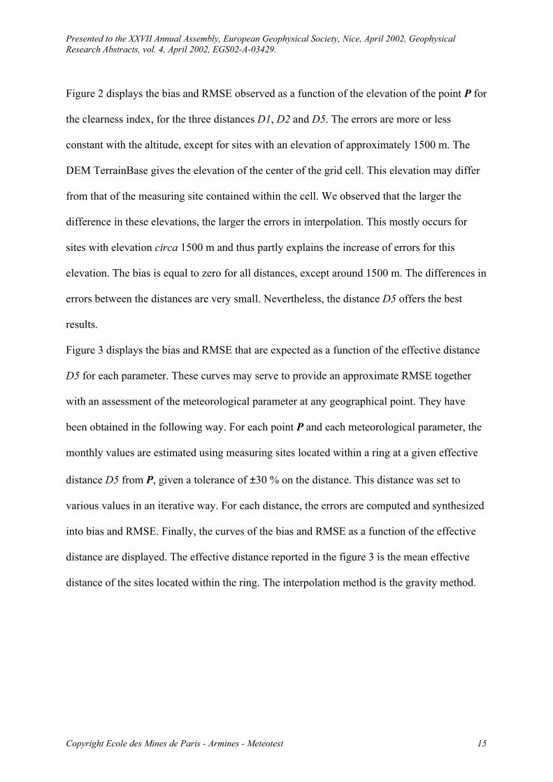
Figure 2. As for Figure 1, but as a function of the altitude (in meters).



Figure 2 displays the bias and RMSE observed as a function of the elevation of the point P for

the clearness index, for the three distances D1, D2 and D5. The errors are more or less

constant with the altitude, except for sites with an elevation of approximately 1500 m. The

DEM TerrainBase gives the elevation of the center of the grid cell. This elevation may differ

from that of the measuring site contained within the cell. We observed that the larger the

difference in these elevations, the larger the errors in interpolation. This mostly occurs for

sites with elevation circa 1500 m and thus partly explains the increase of errors for this

elevation. The bias is equal to zero for all distances, except around 1500 m. The differences in

errors between the distances are very small. Nevertheless, the distance D5 offers the best

results.

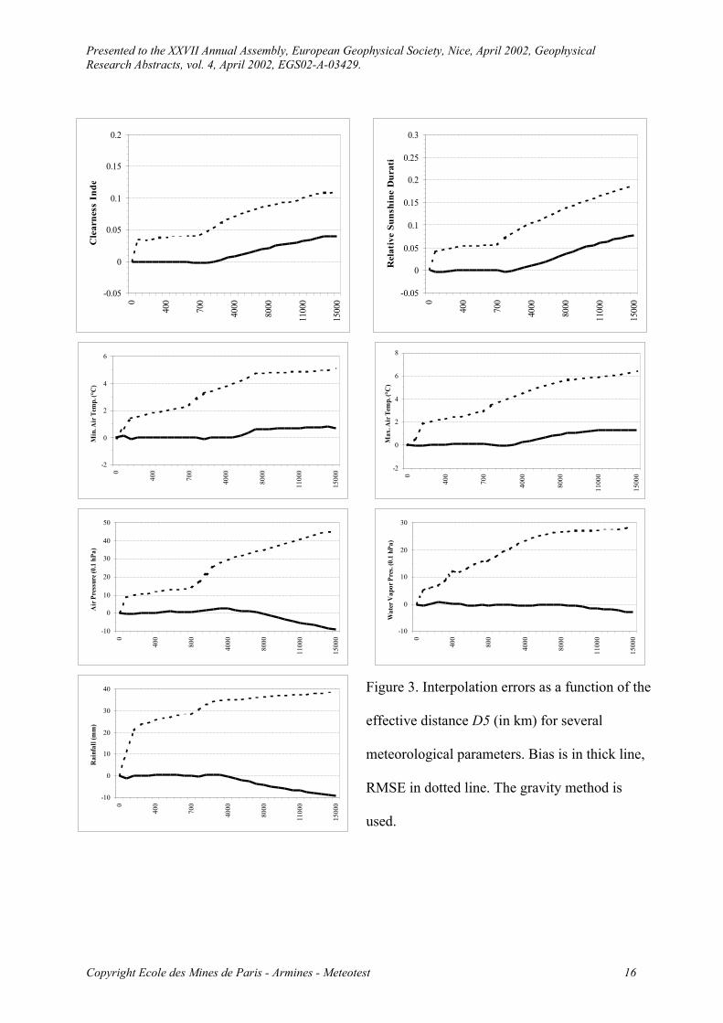
Figure 3 displays the bias and RMSE that are expected as a function of the effective distance

D5 for each parameter. These curves may serve to provide an approximate RMSE together

with an assessment of the meteorological parameter at any geographical point. They have

been obtained in the following way. For each point P and each meteorological parameter, the

monthly values are estimated using measuring sites located within a ring at a given effective

distance D5 from P, given a tolerance of ±30 % on the distance. This distance was set to

various values in an iterative way. For each distance, the errors are computed and synthesized

into bias and RMSE. Finally, the curves of the bias and RMSE as a function of the effective

distance are displayed. The effective distance reported in the figure 3 is the mean effective

distance of the sites located within the ring. The interpolation method is the gravity method.



-0.05

0

0.05

0.1

0.15

0.20

400

700

4000

8000

1100

0

1500

0

Cle

arne

ss I

ndex

-0.05

0

0.05

0.1

0.15

0.2

0.25

0.3

0

400

700

4000

8000

1100

0

1500

0

Rel

ativ

e Su

nshi

ne D

urat

ion

-2

0

2

4

6

0

400

700

4000

8000

1100

0

1500

0

Min

. Air

Tem

p. (°

C)

-2

0

2

4

6

8

0

400

700

4000

8000

1100

0

1500

0

Max

. Air

Tem

p. (°

C)

-10

0

10

20

30

40

50

0

400

800

4000

8000

1100

0

1500

0

Air

Pre

ssur

e (0.

1 hP

a)

-10

0

10

20

30

0

400

800

4000

8000

1100

0

1500

0

Wat

er V

apor

Pre

s. (0

.1 h

Pa)

-10

0

10

20

30

40

0

400

700

4000

8000

1100

0

1500

0

Rai

nfal

l (m

m)

Figure 3. Interpolation errors as a function of the

effective distance D5 (in km) for several

meteorological parameters. Bias is in thick line,

RMSE in dotted line. The gravity method is

used.



CONCLUSION

This work demonstrates that taking into account the latitudinal effects in the distance brings

an increase in the accuracy in interpolation. Such effects have been seldom mentioned in

previous publications. The orographic effects may be partly corrected by adding the weighted

difference in elevation to the geodetic distance.

We recommend the use of the following effective distance between the point P and each of

the measuring sites Xi for all parameters:

deff2 = fNS

2 (dgeo2 + foro

2 δh2) (11)

with fNS = 1 + 0.3 ΦP -ΦX [1+ (sinΦP + sinΦX) / 2], where dgeo is the geodetic distance in

km, latitudes ΦP and ΦX are expressed in degrees, δh is the difference in elevation between P

and Xi (expressed in km) and foro is set to 500.

This distance is identical to the geodetic distance if sites are on the same latitudes and have

the same elevation. If the difference in latitude between the point P and a site Xi is 10° at

45°N, then the effective distance is equal to 6 times the geodetic distance. As for the

difference in elevation, assuming no difference in latitude between the point P and a site Xi

and assuming that the geodetic distance is much larger than (500 δh), the effective distance

may be approximated by:

deff ≈ dgeo [1 + (foro2 δh2 / dgeo

2)/2] (12)

For a difference in elevation of 200 m and a geodetic distance of 200 km, then the effective

distance is equal to 1.1 times the geodetic distance. The larger the geodetic distance, the

smaller the influence of the difference in elevation.

An implementation of this distance was performed within the SoDa service on the Web (SoDa

2001). This prototype service delivers information on solar radiation and related quantities

(Rigollier et al. 2000). The implemented resource serves climatological values of monthly



global irradiation and ambient temperature for any point on Earth within a cell of 5' of arc

angle. The already available gridded climatological databases are used for Europe: ESRA

(2000) and MeteoNorm (2000) for irradiation and MeteoNorm for temperature. Otherwise, a

gravity technique integrating the proposed effective distance is applied. This technique was

selected as a good trade-off between fast answer and accuracy. Meteorological inputs are

taken from the databases of long-term means held in the product MeteoNorm (Remund et al.

1998), originating from the database CliNo of the World Meteorological Organization (WMO

1998), the Global Energy Balance Archive (Gilgen et al. 1998, http://bsrn.ethz.ch/gebastatus/)

and the USA National Solar Radiation Data Base (http://rredc.nrel.gov/solar/old_data/nsrdb/).

There are 1124 stations for the irradiation and 2559 for temperature. The digital elevation

model is the TerrainBase database.

To permit real time answer, the search for stations is limited to a region of 2000 km in radius

(geodetic distance). If no station is present (e.g. ocean parts), the zonal mean value is

computed over a band of 10° in width and is allotted to the site of interest. The quality of the

retrieval is given by previous works as well as the present one. For monthly means of the

temperature, the mean bias error is about 0.1 °C and the RMSE 1.9 °C. For regions with

denser networks like Europe, the RMSE is smaller: about 1 °C (Remund, Kunz, 1997). For

monthly irradiation, the error depends on the source. The gridded data for Switzerland and

Europe were constructed using a dense network and a combination of ground measurements

and satellite data. For Switzerland, the relative RMSE is about 6 % (Remund et al., 1998) and

for Europe, it ranges from 6 % (summer) to 10-15 % (winter) (Beyer et al., 1997). Outside

Europe, where interpolation is called upon, the relative RMSE is about 10 - 15 %.



ACKNOWLEDGEMENTS

The Commission of the European Communities under Contract Number IST-1999-12245

supported this work. Discussions with Hans-Georg Beyer, Tamas Prager and Aniko Rimoczi-

Paal are gratefully acknowledged.

REFERENCES

Anonymous, 1995. Spatial interpolation of daily meteorological data. Report to the Joint Research Centre, Institute for Remote Sensing, Commission of the European Communities.

Anthes R. A., 1997. Meteorology, 7th Edition. Prentice Hall, New Jersey, USA, 214 pp.Atlas of hydrometeorological data – Europe, 1991. In Russian. Published by Army Publishing House,

Moscow, Russia, 371p.Beyer H.-G., Czeplak G., Terzenbach U., Wald L., 1997. Assessment of the method used to construct

clearness index maps for the new European solar radiation atlas (ESRA). Solar Energy, 61, 6, 389-397.

Bresenham J. E., 1965. Algorithm for computer control of digital plotter. IBM Systems Journal, 4(1), 25-30.

Courault D., Monestiez P., 1999. Spatial interpolation of air temperature according to atmospheric circulation patterns in southeast France. International Journal of Climatology, 19(4), 365-378.

ESRA, European Solar Radiation Atlas, 2000. Fourth edition, includ. CD-ROM. Edited by J. Greif, K. Scharmer. Scientific advisors: R. Dogniaux, J. K. Page. Authors: L. Wald, M. Albuisson, G. Czeplak, B. Bourges, R. Aguiar, H. Lund, A. Joukoff, U. Terzenbach, H. G. Beyer, E. P. Borisenko. Published for the Commission of the European Communities by Presses de l'Ecole, Ecole des Mines de Paris, Paris, France.

Gilgen H., Wild M., Ohmura A., 1998. Means and trends of shortwave incoming radiation at the surface estimated from Global Energy Balance Archive data. Journal of Climate, 11, 2042-2061.

Hou H. S., Andrews H. C., 1978. Cubic splines for image interpolation and digital filtering. IEEE Transactions on Acoustic, Speech, and Signal Processing, vol. ASSP-26, 508-517.

Hudson G., Wackernagel H., 1994. Mapping temperature using kriging with external drift: theory and an example from Scotland. International Journal of Climatology, 14, 77-91.

Hulme M., Conway D., Jones P. D., Jiang T., Barrow E.M., Turney C. , 1995. A 1961-1990 climatology for Europe for climate change modelling and impact applications. International Journal of Climatology, 15, 1333-1364.

Hutchinson M.F., Booth T.H., McMahon L.P., Nin H. A., 1984. Estimating monthly mean values of daily total solar radiation for Australia. Solar Energy 32, 277-290.

Jones P. G., Thornton P. K., 1999. Fitting a third-order Markov rainfall model to interpolated climate surfaces. Agricultural and Forest Meteorology, 97(3), 213-231.

Journel A., Huijbregts C., 1978. Mining Geostatistics. Academic Press, London.Kunz S., Remund J., 1995. MeteoNorm - a comprehensive meteorological database and planing tool,

In . 13th European PV-Solar Energy Conference, pp. 733-735, Nice, France.Lo F. K., 1989. Estimation des précipitations à partir de l'analyse utilisant le relief pour

l'hydrométéorologie (AURELHY). Physio-Géo, 19, 37-48.MeteoNorm, version 4.0, 2000. Version 3.0, 1997. Global meteorological database for solar energy

and applied climatology. Published by Meteotest, Bern, Switzerland.Nalder I. A., Wein R. W., 1998. Spatial interpolation of climatic normals. Agricultural and Forest

Meteorology, 92, 211-225.



Picinbono B., 1986. Remarques sur l'interpolation des signaux. Traitement du Signal, 3, 165-170.Price D. T., McKenney D. W., Nalder I. A., Hutchinson M. F., Kesteven J. L., 2000. A comparison of

two statistical methods for spatial interpolation of Canadian monthly mean climate data. Agricultural and Forest Meteorology, 101, 81-94.

Remund J., Kunz S., 1997. Worldwide interpolation of meteorological data. In Proceedings of 14th

Solar Energy Photovoltaic Conference and Exhibition, Barcelona. Volume I, pp. 1059-1061.Remund J., Salvisberg E., Kunz S., 1998. Generation of hourly shortwave radiation data on tilted

surfaces at any desired location. Solar Energy, 62(5), 331-334.Rigollier C., Albuisson M., Delamare C., Dumortier D., Fontoynont M., Gaboardi E., Gallino S.,

Heinemann D., Kleih M., Kunz S., Levermore G., Major G., Martinoli M., Page J., Ratto C., Reise C., Remund J., Rimoczi-Paal A., Wald L., Webb A., 2000. Exploitation of distributed solar radiation databases through a smart network: the project SoDa. EuroSun 2000, June 2000, Copenhagen, Denmark.

� en Z., � ahin A. D., 2001. Spatial interpolation and estimation of solar irradiation by cumulative semivariograms. Solar Energy, 71, 11-21.

SoDa, 2001. SoDa – Integration and exploitation of networked Solar radiation Databases for environment. http://soda.jrc.it.

Supit I., 1994. Global radiation. Published by the European Commission, Office for Official Publications of the European Communities, Luxembourg, CL-NA-15745-EN-C, 194 p.

TerrainBase, 1995. TerrainBase: Worldwide Digital Terrain Data. Documentation Manual, CD-ROM Release 1.0, April 1995. NOAA, National Geophysical Data Center, Boulder, Colorado, USA.

Thiébaux H. J., Pedder M. A., 1987. Spatial Objective Analysis: with applications in atmospheric science. Academic Press, 295 p.

Van der Goot E., 1999. Spatial interpolation of daily meteorological data for the Crop Growth Monitoring System (CGMS). In Proceedings of COST seminar on "Data Spatial Distribution in Meteorology and Climatology", October 1997, (ed. M. Bindi & B. Gozzini), Office for the Official Publications of the European Communities, Luxemburg.

Van der Voet P., Van Diepen C.A., Oude Voshaar J., 1994. Spatial interpolation of daily meteorological data: a knowledge-based procedure for the region of the European Communities. Report 53.3, 118 pp, DLO Winand Staring Centre, Wageningen, The Netherlands.

Willmott C. J., Robeson S. M., 1995. Climatologically aided interpolation (CAI) of terrestrial air temperature. International Journal of Climatology, 15, 221-229.

WMO, 1981. Meteorological aspects of the utilization of solar radiation as an energy source. Technical Note 172, WMO- No 557, World Meteorological Organization, Geneva, Switzerland, 298 p.

WMO, 1998. 1961 – 90 Climatological Normals (Clino). Version 1.0 – November 1998.CD-ROM. World Meteorological Organization, Geneva, Switzerland.

Zelenka A., Czeplak G., d’Agostino V., Josefson W., Maxwell E., Perez R., 1992. Techniques for supplementing solar radiation network data, Technical Report (3 volumes), International Energy Agency, # IEA-SHCP-9D-1, Swiss Meteorological Institute, Krahbuhlstrasse, 58, CH-8044 Zurich, Switzerland.


study of effective distances for interpolation schemes in

Documents