study of associated charmonium j/Ψ production in $\bar{p} p \rightarrow\pi^{0} +j/\varpsi$

$: Study of associated charmonium J/Ψ production in $\bar{p} p \rightarrow\pi^{0} +J/\varPsi$$
Eur. Phys. J. C (2013) 73:2640DOI 10.1140/epjc/s10052-013-2640-2

Regular Article - Theoretical Physics

Study of associated charmonium J/Ψ productionin p̄p → π0 + J/Ψ

Jacques Van de Wiele1,a, Saro Ong1,2

1Institut de Physique Nucléaire, IN2P3-CNRS, Université de Paris-Sud, 91406 Orsay Cedex, France2Université de Picardie Jules Verne, 80000 Amiens, France

Received: 10 June 2013 / Revised: 15 October 2013 / Published online: 26 November 2013© Springer-Verlag Berlin Heidelberg and Società Italiana di Fisica 2013

Abstract The exclusive charmonium production processp̄p → π0 + J/Ψ is investigated for the planned p̄p experi-ment with the PANDA detector at GSI/FAIR. The measuredexclusive cross section of this reaction was reported first bythe E760 and E835 collaborations at Fermilab, in the energyrange (3525 MeV) of charmonium state hc production. Therecent measurements of the charmonium decay widths re-ported by the CLEO and BES collaborations allow one tomake constraints on model assumptions.

1 Introduction

Despite an impressive number of charmonium cc̄ states col-lected by BES [1, 2] and CLEO [3, 4], the strong hadronicdecay widths of charmonium remain poorly understood. Thecrossed reaction, namely charmonium production associatedwith a light meson in pp̄ annihilation, planned at GSI/FAIRwith the PANDA detector [5], appears especially interestingfor a complete description of charmonium properties. Un-til then, the sparse existing data for p̄p → π0 + J/Ψ werereported by E760 [6] and E835 [7, 8] near

√s ∼ 3.5 GeV.

The search of the hc, resonantly formed in pp̄ annihilationis the main objective of these experiments. The measuredcross sections of p̄p → π0 +J/Ψ show no significant eventexcess in the hc (3525 MeV) mass region. However, CLEOand BES reported the observation of the hc in the ηc + γ

decay mode [9, 10].The theoretical study of such a process was first sug-

gested in a PCAC model [11] and the prediction is somewhatlarger than the Fermilab data. The near threshold associatedcharmonium production with a light meson, in pp̄ annihila-tion, is previously investigated in [12, 13], within the frame-work of a non-perturbative effective hadronic theory. Theevidence for a pp̄J/Ψ Pauli strong coupling is pointed out

a e-mail: [email protected]

in [14] and the effect of a Pauli term on the p̄p → π0 +J/Ψ

is quantified. Recently, the authors of Ref. [15] revisitedthese channels by considering the contribution of form fac-tors in the pp̄J/Ψ and pp̄π vertices. But more complicatedLorentz structure at the pp̄J/Ψ vertex, allowing for deriva-tive couplings, is still missing.

In this paper, we develop a nucleon–pole exchange model(Fig. 1), improving on the works of the authors of Refs. [12–15] for p̄p → π0 + J/Ψ , including off-shell hadronic formfactors and a complete Lorentz structure with a Pauli strongcoupling at the pp̄J/Ψ vertex. The effect of replacing thepseudoscalar pp̄π coupling by the pseudovector one is alsoquantified. We adopt the most commonly used form factorsfor the πNN vertex to fit the pion photoproduction in agauge invariant way [16–19]. The values of the few param-eters of our model are extracted from the branching ratio ofthe strong decay mode pp̄ of J/Ψ and the angular distri-bution of this decay in its rest frame, recently measured atBES [2] in e+e− → J/Ψ → pp̄. In Sect. 3, we will showthat this distribution suggests a complete Lorentz structureat the pp̄J/Ψ vertex. We assume that the nucleon–pole di-agram is the dominant one and neglect the contribution ofother baryon resonances as a first application. However, it isknown that in low energy processes such as J/Ψ → π0pp̄,the partial wave analysis suggests the dominance of the de-cay Dalitz plot by a few baryon resonances with masses upto 2.0 GeV [1]. The analysis of this decay channel is be-

Fig. 1 Feynman diagrams for the nucleon–pole model in p̄p →π0 + J/Ψ ; R is a generic charmonium state

mailto:[email protected]

Page 2 of 14 Eur. Phys. J. C (2013) 73:2640

ing undertaken, and the nucleon–pole contribution is largelyemphasized in the soft-pion limit [20]. The resulting decaywidth is very sensitive to the model assumption of the off-shell hadronic form factors [21].

In Sect. 4, we also estimate the contribution of possibleintermediate resonances reported by BES [1] in J/Ψ →pp̄π0 decay analysis. This development is needed to de-scribe the data of such decays where the N∗ resonance peaksare clearly observed. The incorporation of these resonancesis complicated, as it will introduce new resonance couplingparameters and nontrivial phases. To draw firm conclu-sions in this work, we include N(1440),N(1520),N(1535),N(1650),N(1710) with JP = 1/2+,3/2−,1/2−, 1/2−,1/2+,respectively.

Recently, the hadronic structure in terms of the funda-mental degrees of freedom of QCD, has been analyzed inthe framework of the collinear factorization theorem [22, 23]with the new non-perturbative objects, the so-called transi-tion distribution amplitudes (TDAs) [24, 25]. The reactionp̄p → π0e+e− in the kinematical regime of high invariantmass of the lepton pair is analyzed in this framework to ex-tract the baryon to meson transition distribution amplitude[26]. Assuming that M2

J/Ψ = 9.6 GeV2 is high enough toassure the hard scale of QCD, the TDA formalism will bringa new perspective to study the associated charmonium J/Ψ

production in pp̄ annihilation. It will be interesting to com-pare the predictions of nucleon–pole exchange model to theTDA formalism [27].

2 Model of the associated charmonium production

We assume that at tree level, this process is described by thenucleon–pole diagrams of Fig. 1. In order to estimate thecross section of the p̄p → π0 + J/Ψ reaction, we need tospecify the hadronic interaction Lagrangian of nucleons andJ/Ψ :

LV NN

= −K

[Ψ p

(γμ − κ

2Mσμν∂

ν

)V μ

]Ψp (1)

where V is the vector charmonium field, M the nucleonmass and K,κ are complex quantities.

We made calculations with both pseudovector and pseu-doscalar nucleon–pion interaction. The interaction Lagrang-ians are given by

LPVπNN

= −gπNN

2MΨ pγ5γμτ · ∂μπΨp (2)

LPSπNN

= −igπNNΨ pγ5τ · πΨp (3)

where τ and π are the isospin Pauli matrix and the pionfield, respectively. gπNN is the pion–nucleon coupling con-stant with g2

πNN/4π = 12.562. The effect of replacing thepseudoscalar coupling by the pseudovector one in the casewhere κ �= 0 is studied.

2.1 Kinematics

Let us first introduce our notation for the annihilation pro-cess: p̄(p̄) + p(p) → π0(pπ ) + J/Ψ (q). The quantities inbracket are the corresponding four-momentum of the parti-cles, with

p̄ + p = pπ + q (4)

p̄2 = p2 = M2, p2π = M2

π , q2 = M2J/Ψ (5)

s = (p̄ + p)2, t = (p̄ − pπ)2, u = (p̄ − q)2 (6)

s + t + u = 2M2 + M2J/Ψ + M2

π (7)

Defining

q1 = p − pπ, q2 = pπ − p̄ (8)

d1 = q21 − M2 = u − M2 (9)

d2 = q22 − M2 = t − M2 (10)

We also display some useful relations between the kine-matical quantities

p̄ · p = s

2− M2 (11)

p̄ · pπ = M2 + M2π − t

2(12)

p̄ · q = M2 + M2π − u

2= s + t − M2 − M2

π

2(13)

p · pπ = M2 + M2π − u

2= s + t − M2 − q2

2(14)

p · q = p · (p̄ + p − pπ) = M2 + q2 − t

2(15)

q1 + q2 = p − p̄ (16)

q1 · q2 = 2M2 − q2 − M2π

2(17)

To justify the model assumptions of the nucleon–pole forp̄p → π0 + J/Ψ , we display in Fig. 2, the kinematicallyallowed region of the (πp) or (πp̄) invariant mass squarewhich is a function of Ecm = √

s. In the energy range ofour interest, the maximum value of the q2

1 or q22 is less than

the mass square of the nucleon. A first estimate of the crosssection, neglecting the contribution of other baryons withmasses up to 2 GeV is therefore meaningful.

2.2 Amplitudes and cross sections

The amplitude contains the two contributions from the dia-grams of Fig. 1

Eur. Phys. J. C (2013) 73:2640 Page 3 of 14

Fig. 2 Kinematical allowed region for the momentum of exchangedbaryons in p̄p → π0 + J/Ψ versus Ecm (Color figure online)

M(λ;mp̄,mp) = M(1;λ;mp̄,mp)

+M(2;λ;mp̄,mp) (18)

M(i;λ;mp̄,mp) = v̄p̄(mp̄)Γ μ(i)up(mp)ε∗μ(λ) (19)

Here εμ(λ) denotes the polarization vector of the J/Ψ

and i = 1, 2 is the number of the diagram in Fig. 1.The contribution of the diagram (1), with q1 = p − pπ

and the diagram (2), with q2 = pπ − p̄ are written in termsof Γ μ(1) and Γ μ(2) given below.

Γ μ(1) = VμNNJ/Ψ iPF (N;q1)VNNπ (20)

Γ μ(2) = VNNπ iPF (N;q2)VμNNJ/Ψ (21)

The nucleon propagator is

PF (N;qi) = /qi + M

q2i − M2

(22)

For the pseudoscalar πNN coupling, we have

VNNπ = gpsπNNCπNN

isos γ 5 (23)

gpsπNN = √

4π × 12.562, CπNNisos = 1 (24)

The pseudovector πNN coupling requires

VNNπ = gpvπNNCπNN

isos γ 5/pπ (25)

gpvπNN = g

psπNN

2M, CπNN

isos = 1 (26)

VμNNJ/Ψ = −iK

(γ μ − i

κ

2Mσμνqν

)(27)

In the above, the coupling constant of the J/Ψ NN interac-tion, namely gJ/Ψ NN , is included in the parameter K . Forthe physics meaning of the parameters K and κ , one can

compare with VμNNγ where the J/Ψ is replaced by the pho-

ton:

VμNNγ = −iep

(F

p

1 γ μ − iF

p

2

2Mσμνqν

)(28)

From this point of view, K and Kκ are related to theequivalent Dirac and Pauli electromagnetic form factors. Inthe time-like region, F

p

1 and Fp

2 as well as K and κ , arecomplex quantities.

Now, let us define the hadronic current:

JμH (mp̄,mp) = v̄p̄(mp̄)Γ μup(mp) (29)

with

Γ μ = Γ μ(1) + Γ μ(2) (30)

The amplitude of the process is given by

M(λ;mp̄,mp) = JμH (mp̄,mp)ε∗

μ(λ) (31)∣∣M(λ;mp̄,mp)

∣∣2 = JμH (mp̄,mp)J ν

H∗(mp̄,mp)

× ε∗μ(λ)εν(λ) (32)

∑λ,mp̄,mp

∣∣M(λ;mp̄,mp)∣∣2 = Hμν

∑λ

ε∗μ(λ)εν(λ) (33)

The sum is performed over all different spin components ofJ/Ψ , p̄ and p. Hμν is the hadronic tensor, defined as

Hμν =∑

mp̄,mp

JμH (mp̄,mp)J ν

H∗(mp̄,mp) (34)

In the C.M system, the beam direction of p̄ is taken asthe Oz axis

Ep̄ = Ep =√

s

2(35)

|p̄| = |p| =√

s(1 − 4M2/s)

2(36)

|pπ | =√

(s − (MJ/Ψ + Mπ)2)(s − (MJ/Ψ − Mπ)2)

2√

s(37)

d2σ

dΩπ

= 1

64(2π)2s

|pπ ||p̄|

∑λ,mp̄,mp

∣∣M(λ;mp̄,mp)∣∣2 (38)

In terms of K and κ , the differential cross section reads

d2σ

dΩπ

= 1

64(2π)2s

|pπ ||p̄| |K|2(A + B|κ| cosϕκ + C|κ|2)

(39)

Here κ = |κ| exp(iϕκ), and the analytical expressions of thecross section, in particular the quantities A, B , and C in


(39), have been derived with the help of Mathematica [28].A cross check in calculating numerically these amplitudeshas been done. In Appendix, we write down the differentterms in the expression of the cross section in the pseu-doscalar and pseudovector (πNN) nucleon–pion interac-tion with the appropriate hadronic form factors. We havechecked analytically that the same expression occurred forboth cases when κ = 0.

For comparison with the previous work [13], we expressthe differential cross section given in Appendix in the casewhere κ = 0, namely G2 = 0, w1 = w2 = 1 (no form factorsincluded) and in the massless pion limit to reproduce exactlythe formula (4) in [13]:

dσ

dt= |K|2(gps

πNN)2

16πs(s − 4M2)

(s − 4M2J/Ψ )2

(t − M2)(u − M2)(40)

2.3 Hadronic form factors

It is well known that the hadronic form factors play an im-portant role in many processes, in particular in pion pho-toproduction, πN and NN scatterings. The off-shellness ofthe exchanged baryon in the model assumption, is taken intoaccount by implementing these form factors at each meson–baryon–baryon vertex. However, the hadronic form factorsare commonly adopted phenomenologically [29–31]. Theireffects could reduce substantially the predicted cross sectionand the lack of the available data does not allow one to de-termine the form factors without ambiguities. In the presentstudy, we adopt the dipole form with the parameter Λ

FD

(Q2) = 1

1 + (Q2 − M2)2/Λ4(41)

where Q2 is the momentum squared of the off-shell ex-changed particle in the diagrams of Fig. 1.

In order to respect the Fermilab data, a reasonable valueof this unique parameter is ΛPS = 1.25 GeV for the pseu-doscalar (πNN) nucleon–pion interaction and ΛPV =1.35 GeV for the pseudovector one.

One should incorporate N∗ resonances with appropri-ate hadron vertex form factors which are poorly known. Toquantify the effect of these resonances, we adopt in Sect. 4,a minimal free parameters model with hadronic form fac-tors for the off-shell nucleon exchanged as well as the reso-nances.

3 Estimating the pp̄J/Ψ coupling constantsfrom decay width

The coupling constant of the J/Ψ to pp̄ is not well estab-lished. With the complete Lorentz structure given in the ex-pression of the Lagrangian (Eq. (1)), the two parameters,

namely K and κ , are complex quantities. The recent precisemeasurements of the J/Ψ → pp̄ decay width and the dis-tribution of the angle between the proton and the beam di-rection, reported by the BES collaboration [2], are sensitiveto the moduli of these parameters and cosϕκ , where ϕκ isthe phase of κ . The decay width Γ of J/Ψ → pp̄ is relatedto the parameters K and κ by

|K|2 = 12πΓ (J/Ψ → p̄p)

MJ/Ψ

(1 − 4M2/M2J/Ψ

)3/2G(M2J/Ψ

,M2, κ)(42)

G(M2

J/Ψ,M2, κ

) = NM2

J/Ψ(1 − 4M2/M2

J/Ψ)

(43)

N = 2M2 + (1 + 3|κ| cosϕκ + |κ|2)M2

J/Ψ

+ |κ|2M4J/Ψ

/8M2 (44)

The angular distribution of the proton in the rest frame ofthe J/Ψ of the process e+e− → J/Ψ → p̄p takes on thesimple form

dσ

dΩ∼ 1 + α cos2 θ

The parameter α is given in our model by

α(|κ|, cosϕκ

) = Nα

Dα

(45)

where

Nα = −16M4 + 4M2q2 + 4M2|κ|2q2 − |κ|2q4 (46)

Dα = 16M4 + 4M2q2 − 16 cosϕκM2|κ|q2

+ 4M2|κ|2q2 + |κ|2q4 (47)

with q2 = M2J/Ψ .

However, the measured value of α = 0.595 ± 0.012 ±0.015 [2] in the angular distribution, suggests a non-zerovalue of the κ . For κ = 0, the expected value would havebeen

α0 = q2 − 4M2

q2 + 4M2= 0.463

With these two constraints from experimental values ofΓ (J/Ψ → p̄p) � 0.2 keV and α � 0.6, we are able togive a set of K and κ values in a reasonable agreementwith the Fermilab data (E760 and E835) for the reactionpp̄ → π0 + J/Ψ .

The value of |κ| is a solution of Eq. (45), where the cosϕκ

is a parameter. To satisfy the constraint for a possible solu-tion of this second order equation in |κ|, the only parameterof this equation should be

cos2 ϕκ ≥ (q2 + 4M2)2(α2 − α20)

16q2M2α2(48)


This also requires that α ≥ α0. With the measured valueof α � 0.6, this positive solution of |κ| exists for cosϕκ ≥0.7178. However, K has a nontrivial phase. The allowed re-gions for moduli of K and κ are displayed in Fig. 3. Thisexplains some values of cosϕκ , |κ| and |K| displayed in Ta-ble 1.

The authors of Ref. [14] express the parameters K andκ of the model in terms of Sachs form factors GE and GM

with

GE = K(1 + κq2/4M2), GM = K(1 + κ)

Assuming the Sachs form factor ratio GE/GM =ρ exp(iχ) as a complex parameter, the relation between κ

and this ratio reads

κ = |κ| exp(iϕκ) = ρ exp(iχ) − 1

q2/4M2 − ρ exp(iχ)(49)

The parameter α in the angular distribution of the proton inthe rest frame of the J/Ψ in e+e− → J/Ψ → p̄p is relatedto the ratio ρ in a simple form

α = 1 − (4M2/q2)ρ2

1 + (4M2/q2)ρ2(50)

Fig. 3 Allowed regions for moduli of K and κ . The dashed and solidlines correspond to the two solutions of Eqs. (45) and (42)

Table 1 Set of different values of K and κ in the model

Γ (J/Ψ → pp̄) � 0.2 keV, α = 0.6

cosϕκ |κ| |K|

0.0000 0.0000 1.617 × 10−3

0.7178 0.2176 1.325 × 10−3

1.0000 0.0921 1.446 × 10−3

1. 0000 0.5143 0.961 × 10−3

In conclusion, we claim that the phase of K is unconstrainedregarding the measured value of α in agreement with theprevious work [14]. However, for the Pauli coupling con-stant κ , we obtain a correlation between the moduli of κ andhis phase ϕκ through the relation (45) in the present work,similar to those of [14] in the following form:

ρ2 = 1 + |κ|2q4/16M4 + (2|κ|q2/4M2) cosϕκ

1 + |κ|2 + 2|κ| cosϕκ

(51)

For this reason, one obtains for a fixed value of the cosϕκ ,two possible values of |κ|, in Table 1.

In the reaction J/Ψ → pp̄π0, the partial wave analysisof this decay suggests the contribution of baryon resonanceswith masses up to 2.0 GeV [1]. This feature can be explainedby the kinematical domain allowed for the invariant mass W

of the (πp) and (πp̄) system, namely Wmin = M + Mπ andWmax = MJ/Ψ − M .

The values of |K| and |κ| in Table 1 are obtained with-out consideration of the decay width Γ (J/Ψ → p̄pπ0). Wewill show in the next section, the comparison between thenucleon–pole model and its extension including intermedi-ate N∗ resonances.

Let us emphasize again the non-zero value of the param-eter κ in this effective Lagrangian model to obtain the cor-rected coefficient α ≥ α0 in the angular distribution of theJ/Ψ → pp̄ decay. In principle, this measured value of α

[2, 33, 34] permits discrimination among the different theo-retical models [35–37].

4 Intermediate N∗ resonances contribution

A generalization of the nucleon–pole model, incorporat-ing intermediate N∗ resonances, is pointed out in [32] forJ/Ψ → p̄pπ0. For the first time, the study of their effectin the crossed channel, namely p̄p → π0 + J/Ψ is con-sidered in this present work. The partial wave analysis ofJ/Ψ → p̄pπ0 [1] is performed to study the N∗ states. Thesequential decay process is described by the Feynman dia-grams in Fig. 4. According to the results of [1], we adopt aset of resonances with well established masses, widths andspin parity JP . The contribution of resonances (with isospin

Fig. 4 Feynman diagrams of J/Ψ → p̄pπ0, N∗ (N̄∗) is the interme-diate baryon resonance considered in the model


I = 1/2) to the decay width of J/Ψ → p̄pπ0 is shown inTable 2 with the fraction in % of each resonance.

This development is crucial to describe the BES data,however, one should introduce many new and poorly knownresonance coupling constants and phases.

To estimate the contribution of these resonances to thep̄p → π0 + J/Ψ reaction, we have chosen the most sim-ple Lagrangians to be limited to a small number of free pa-rameters. For the nucleon, the pseudoscalar coupling πNN

was chosen (Eq. (3)) and the J/Ψ NN coupling was takenwith κ = 0. The fractions displayed in Table 2 allow oneto determine the coupling constants of different vertices(NN∗J/Ψ ), assuming the Lagrangians for the consideredresonances, as given in [38]:

LPSπNP11

= −iKπNP11Ψ pγ5τ3π0ΨP11 + h.c. (52)

KπNP11 = (M + MP11

)√

g × 4π

g ={

0.510 P11(1440)

0.012 P11(1710)

(53)

LPSπNS11

= −iKπNS11Ψ pτ3π0ΨS11 + h.c. (54)

KπNS11 = √g × 4π

g ={

0.037 S11(1535)

0.060 S11(1650)

(55)

LπND13

= KπND13Ψ pγ5γμτ3(∂μ∂νπ0)gανΨ

αD13

+ h.c. (56)

KπND13(1520) = √1.73 × 4π (57)

LV NP11

= −gV NP11

Ψ pγμτ3VμΨP11 + h.c. (58)

where V μ is the vector charmonium field.

LV NS11

= −gV NS11

Ψ pγ5γμτ3VμΨS11 + h.c. (59)

LV ND13

= −igV ND13

Ψ pγνFνμτ3gαμΨ α

D13+ h.c. (60)

Fνμ = ∂μV ν − ∂νV μ (61)

The coupling constants at the J/Ψ NP11, J/Ψ NS11 andJ/Ψ ND13 vertices were adjusted to reproduce the BES par-tial widths (Table 2) assuming no interference in the cal-culation. In the analysis of the BES data, the authors givelarge uncertainties in the final partial widths in particularfor the P11(1710) resonance. In the calculation of the decayJ/Ψ → p̄pπ0 including the interference terms, the cou-pling constant for the P11(1710) was reduced to get a partialwidth to 5 % instead of 25.33 %. With these parameters, acoherent calculation of the amplitudes has been performed.We reproduce qualitatively (Fig. 5) the Mpπ0 invariant mass

Table 2 Summary of N∗ states considered in the model

Γ (J/Ψ → pp̄π0) = 1.09 × 10−3, Γtot = 93 keV

N∗ (mass in MeV) Width (MeV) JP Fraction

N(1440) 316 12

+16.37

N(1520) 127 32

−7.96

N(1535) 135 12

−7.58

N(1650) 145 12

−9.06

N(1710) 95 12

+25.33

Fig. 5 dΓ/dMpπ versus the invariant mass Mpπ . Data from BES [1],red line is the nucleon contribution and the black line is the total con-tribution including resonances (Color figure online)

spectrum measured by the BES collaboration. The branch-ing ratio obtained Br(J/Ψ → pp̄π0) = 1.26 × 10−3 is inagreement with the BES result (1.33 ± 0.02 ± 0.11) × 10−3

[1].As it can be seen in Fig. 5, at least one resonance with

a mass greater than 1.8 GeV is necessary to reproduce thespectrum at large invariant mass values.

In the reaction of our interest, namely p̄p → π0 + J/Ψ ,the effects of these resonances versus nucleon–pole modelalone are displayed in Sect. 5.3.

5 Numerical results

The sparse existing data from Fermilab (E760, E835) areonly sufficient to give us the order of magnitude of the totalcross section. We need to take an average over different binsclose in energy, in Figs. 6 and 7, to make possible a compar-ison with the prediction of our model. We do not try to geta perfect fit of the data in order to leave room for upcom-ing data from PANDA. Both total cross section and differ-ential cross section measurements are needed to make a reli-able conclusion. At this stage of our investigation, we prefer


Fig. 6 Total cross section versus Ecm for p̄p → π0 + J/Ψ , assum-ing pseudoscalar (πNN) coupling. The color line of different curvescorrespond to the parameter values in Table 1. Model without hadronicform factor: (a), and with dipole form factor: (b). Data are taken from[6–8] (Color figure online)

Fig. 7 Total cross section versus Ecm for p̄p → π0 + J/Ψ , assum-ing pseudovector (πNN) coupling. The color line of different curvescorrespond to the parameter values in Table 1. Model without hadronicform factor: (a), and with dipole form factor: (b). Data are taken from[6–8] (Color figure online)

to take only a small number of parameters in our model tofit the available data. In the same spirit, the contribution ofN∗ resonances is quantified, assuming a pure pseudoscalarNN∗π coupling and the simplest Dirac matrix at the vertexNN∗J/Ψ , a pure vector vertex.

5.1 Total cross section without N∗ resonances

We display in Figs. 6 and 7 the predictions of the total crosssection of p̄p → π0 + J/Ψ . The red square points are theE760 data [6] and the black circles, the E835 data [7, 8].

At full integrated luminosity of 2 fb−1 and√

s =3.5 GeV, planned at FAIR/PANDA, a number of ∼5000events is expected for the reaction p̄p → π0 + J/Ψ →π0 + (e+e−). At

√s = 4.5 GeV, this number of events

should decrease by about a factor of 2. This suggests thepossibility to measure both the total cross section and the an-gular distribution at relatively high energy with the PANDAdetector at FAIR.

In our model, the sensitivity to the form factors couldbe sizable at high energy in the relevant PANDA energyregime. The discrimination between the pseudoscalar andpseudovector πNN couplings seems to be a difficult task.However, one can also remark, at high energy, the inversionof different curves in Fig. 7 assuming pseudovector πNN

coupling. It means that the sensitivity to the |K| and |κ| isnot the same for these two possible couplings.

5.2 Angular distribution without N∗ resonances

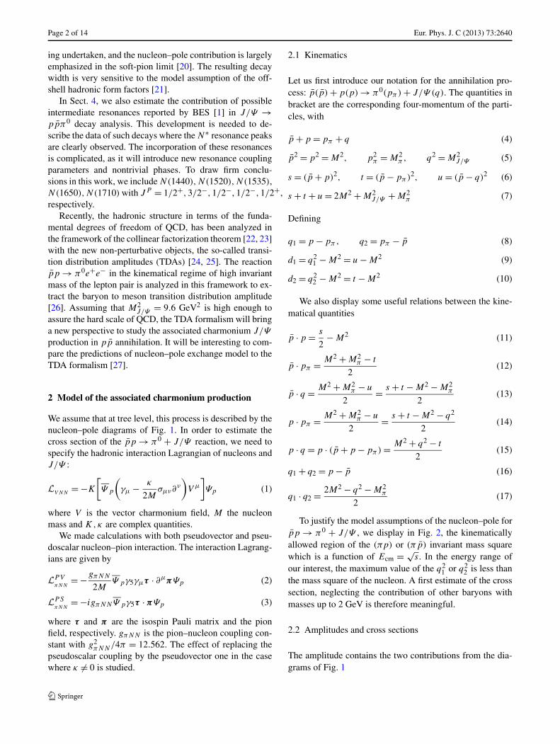
Until now, no data exist for the angular distribution ofp̄p → π0 +J/Ψ . The differential cross section displayed inFigs. 8, 9, 11, 12, where θ is the scattering angle of the pionin the center of mass frame, shows a forward and backwardpeaking with increasing energy. The peak is more importantin the case of pseudoscalar πNN coupling. This differentbehavior is emphasized in the case where the hadronic formfactors are included in the model.

To quantify the effect of replacing the pseudoscalarNNπ coupling by the pseudovector one, we display inFig. 10 the ratio between the differential cross sections ex-hibited in Figs. 9 and 12, for cosϕκ = 1.0000, |κ| = 0.0921and |K| = 1.446 × 10−3. The ratios predicted in Fig. 10permit the discrimination between these two couplings andshould be seen in the planned charmonium experiment atFAIR/GSI with the PANDA detector.

At forward and backward angles, the cross section is re-spectively dominated by the t and u channels and the effectof the hadronic form factor (Eq. (41)) is small. In contrast,at 90 degrees,where Q2 = t = u, both quantities t −M2

B andu − M2

B , where MB is the mass of the exchange baryon, arelarge and the cross section is reduced drastically. At highenergy, the hadronic form factor effect becomes more im-portant.

In summary, we propose to measure the total cross sec-tion for hadronic form factors validation and the angulardistribution to disentangle the pseudoscalar from the pseu-dovector πNN coupling.

5.3 N∗ resonances contribution

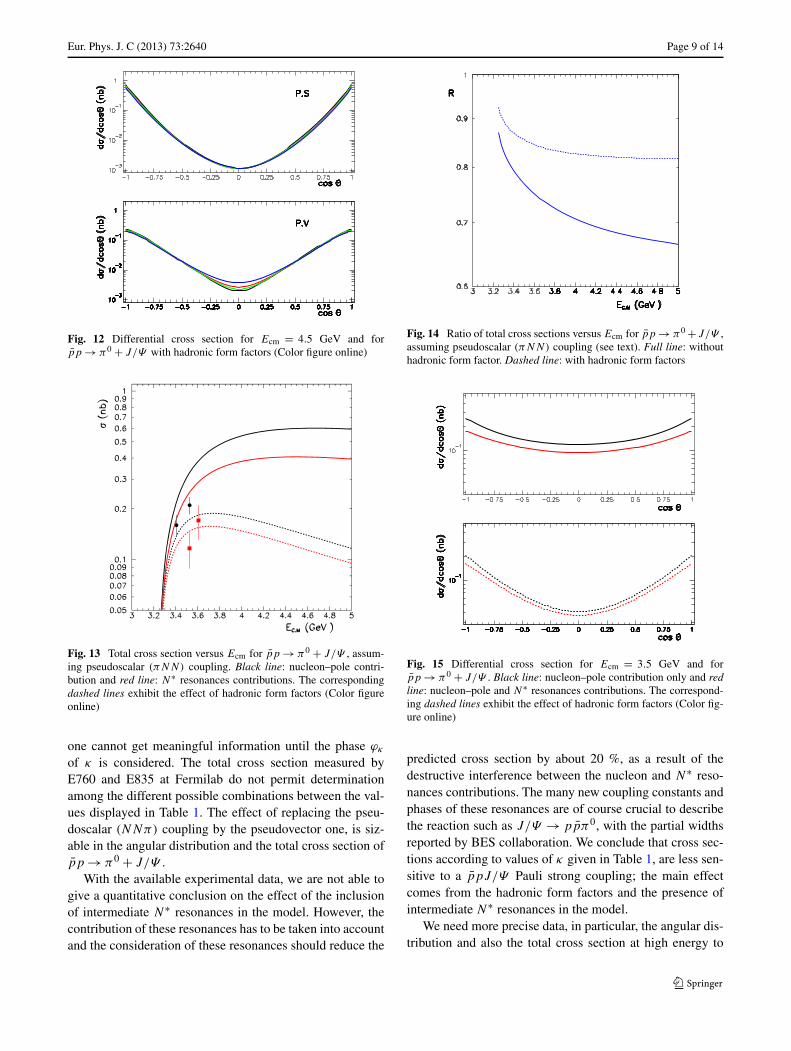
The predictions of the total cross section and the angulardistribution in our model, including N∗ resonances, are dis-played in Figs. 13 and 15. They exhibit a destructive inter-ference between the nucleon and resonances contributions,


Fig. 8 Differential cross section for Ecm = 3.5 GeV and forp̄p → π0 + J/Ψ without hadronic form factors (Color figure online)

Fig. 9 Differential cross section for Ecm = 3.5 GeV and forp̄p → π0 + J/Ψ with hadronic form factors (Color figure online)

as a result of the relative phases chosen for these resonancesin order to respect the BES results in the crossed channelJ/Ψ → p̄pπ0. One also remarks a similar effect from theresonances contribution as well as the hadronic form factorimplementation.

The ratio of the total cross section calculated with nu-cleon and resonances contributions over the total cross sec-tion with nucleon–pole only is displayed in Fig. 14. Thisratio decreases with the energy as it can be seen. Withouthadronic form factor the contribution of the resonances canbe larger than 30 % and with the hadronic form factor thiscontribution becomes smaller than 20 %.

At 3.5 GeV, the form factor effect is smaller than the un-certainties on the data.

Fig. 10 Ratio between differential cross sections assuming the pseu-doscalar and pseudovector (NNπ) coupling, with hadronic form fac-tors included. Ecm = 3.5 GeV (solid line) and Ecm = 4.5 GeV (dashedline)

Fig. 11 Differential cross section for Ecm = 4.5 GeV and forp̄p → π0 + J/Ψ without hadronic form factors (Color figure online)

Let us emphasize that one cannot ignore the contribu-tion of the N∗ resonances in p̄p → π0 + J/Ψ . We needmore precise data, especially the forthcoming data from theplanned p̄p experiment at GSI/FAIR with the PANDA de-tector, to make a consistent conclusion.

6 Conclusions

Our predictions for cross sections in a hadronic-pole model,depend only on the three parameters: K , κ for the (NNJ/Ψ )

coupling constants and Λ for the hadronic form factor as-sumption. In principle, K , κ are complex quantities and


Fig. 12 Differential cross section for Ecm = 4.5 GeV and forp̄p → π0 + J/Ψ with hadronic form factors (Color figure online)

Fig. 13 Total cross section versus Ecm for p̄p → π0 + J/Ψ , assum-ing pseudoscalar (πNN) coupling. Black line: nucleon–pole contri-bution and red line: N∗ resonances contributions. The correspondingdashed lines exhibit the effect of hadronic form factors (Color figureonline)

one cannot get meaningful information until the phase ϕκ

of κ is considered. The total cross section measured byE760 and E835 at Fermilab do not permit determinationamong the different possible combinations between the val-ues displayed in Table 1. The effect of replacing the pseu-doscalar (NNπ) coupling by the pseudovector one, is siz-able in the angular distribution and the total cross section ofp̄p → π0 + J/Ψ .

With the available experimental data, we are not able togive a quantitative conclusion on the effect of the inclusionof intermediate N∗ resonances in the model. However, thecontribution of these resonances has to be taken into accountand the consideration of these resonances should reduce the

Fig. 14 Ratio of total cross sections versus Ecm for p̄p → π0 +J/Ψ ,assuming pseudoscalar (πNN) coupling (see text). Full line: withouthadronic form factor. Dashed line: with hadronic form factors

Fig. 15 Differential cross section for Ecm = 3.5 GeV and forp̄p → π0 + J/Ψ . Black line: nucleon–pole contribution only and redline: nucleon–pole and N∗ resonances contributions. The correspond-ing dashed lines exhibit the effect of hadronic form factors (Color fig-ure online)

predicted cross section by about 20 %, as a result of thedestructive interference between the nucleon and N∗ reso-nances contributions. The many new coupling constants andphases of these resonances are of course crucial to describethe reaction such as J/Ψ → pp̄π0, with the partial widthsreported by BES collaboration. We conclude that cross sec-tions according to values of κ given in Table 1, are less sen-sitive to a p̄pJ/Ψ Pauli strong coupling; the main effectcomes from the hadronic form factors and the presence ofintermediate N∗ resonances in the model.

We need more precise data, in particular, the angular dis-tribution and also the total cross section at high energy to


make serious constraints on the model. The planned p̄p

experiment at GSI/FAIR with the PANDA detector, shouldcontribute to clarify the issue.

The first possibility to fix the phase of κ is from angulardistribution study of leptonic J/Ψ decays in its rest frame,through the process p̄p → π0 + J/Ψ . This topic is largelyemphasized in the feasibility studies of the nucleon time-likeelectromagnetic form factors measurements in the unphysi-cal region with the PANDA detector at FAIR [39, 40]. Thesecond one may be determined through a study of the polar-ized process e+e− → J/Ψ → p̄p [14].

Acknowledgements The authors would like to thank the OR-SAY/PANDA Collaboration members for constructive remarks andconstant encouragements, in particular T. Hennino and R. Kunne for acareful reading of the manuscript.

Appendix: Explicit expressions of different termsin the cross section

Here, we give an explicit expression of the differential crosssection, in a general case assuming the pseudo scalar andpseudo vector(NNπ) coupling.

Defining

x = p · pπ, y = p̄ · pπ, z = p̄ · p (62)

G1 = K, G2 = Kκ (63)

d1 = u − M2, d2 = t − M2, q2 = M2J/Ψ (64)

The sum over the spin states is a polynomial in the pionmass Mπ0 :

∑λ,mp̄,mp

∣∣M(λ;mp̄,mp)∣∣2 =

∑i=0,2,4,6,8 C(i)Mi

π0

d21d2

2

(65)

C(i) = A(i)11 G1G

∗1 + A

(i)12 G1G

∗2/(4M)

+ A(i)21 G2G

∗1/(4M)

+ A(i)22 G2G

∗2/

(16M2) (i = 0,2,4,6,8) (66)

With

A(i)12 = A

(i)21 (67)

The expressions of C(i) reduce to

C(i) = A(i)11 |K|2 + 2A

(i)12 |K|2|κ| cosϕκ/(4M)

+ A(i)22 |K|2|κ|2/(16M2) (68)

A(i)mn = K(i)

mn

{d2

2w21f

(i)mn(x, y, z) + d2

1w22f

(i)mn(y, x, z)

+ d1d2w1w2g(i)mn(x, y, z)

}(m,n = 1,2) (69)

w1 and w2 are hadronic form factors (41) where Q2 is themomentum square of the exchanged nucleon in diagrams 1and 2 of Fig. 1, respectively.

The expression of the differential cross section given in(39) exhibits the κ dependence with it phase ϕκ . The threefunctions A, B , and C are related to the A

(i)11 , A

(i)12 , and A

(i)22

given above:

A =∑

i=0,2,4,6,8

A(i)11 Mi

π/(d2

1d22

)(70)

B = 1

2M

∑i=0,2,4,6,8

A(i)12 Mi

π/(d2

1d22

)(71)

C = 1

16M2

∑i=0,2,4,6,8

A(i)22 Mi

π/(d2

1d22

)(72)

A.1 Pseudoscalar coupling

For i = 0:

K(0)11 = 16(g

psπNN)2

q2(73)

f(0)11 (x, y, z) = x

(q2y + x

(M2 + z

))(74)

g(0)11 (x, y, z) = −2xy

(M2 − q2 + z

)(75)

K(0)12 = 16

(g

psπNN

)2 (76)

f(0)12 (x, y, z) = 3M(x + y)x (77)

g(0)12 (x, y, z) = M(x + y)2 (78)

K(0)22 = 16(g

psπNN)2

q2(79)

f(0)22 (x, y, z)

= 4x[2M4x − q2y

(q2 + 3(x + y)

)+ M2(q2(x + 3y) − 2x(x + y − 2z)

)+ (−2x(x + y) + q2(x + 3y)

)z + 2xz2] (80)

g(0)22 (x, y, z)

= 8[2M4(x2 + xy + y2) − 2M2

(x3 − q2xy + 2x2y + 2xy2 + y3

− (x2 + y2)z) + xy

(−(q2(q2 + x + y

))+ 2

(q2 + x + y

)z − 2z2)] (81)

For i = 2:

K(2)11 = 8(g

psπNN)2

q2(82)

f(2)11 (x, y, z) = −[

2M2(q2 + x) + (

q2 + 2x)z]

(83)


g(2)11 (x, y, z) = 2

[M2(−q2 + x + y

) + (x + y)z]

(84)

K(2)12 = −8

(g

psπNN

)2(85)

f(2)12 (x, y, z) = 3M

[2M2 + x − y + 2z

](86)

g(2)12 (x, y, z) = 4M

(M2 + z

)(87)

K(2)22 = −8(g

psπNN)2

q2(88)

f(2)22 (x, y, z)

= 4[4M6 − 3q2xy − M4(q2 + 4x + 8y − 8z

)− (

q4 + q2x + 6x2 + 3q2y + 4xy)z

+ (3q2 + 4x

)z2

+ M2(2q4 − 2x2 + 4xy + 4(y − z)2

+ q2(3x + y + 2z))]

(89)

g(2)22 (x, y, z) = 8

[4M6 − M4(3q2 + 2(x + y − 4z)

)+ 2z

(x2 + 3xy + y2 − (x + y)z

)+ q2(−xy + z2)+ M2(q4 + 4q2(x + y)

− 2(2x2 + 3xy + 2y2) − 2q2z

− 4(x + y)z + 4z2)] (90)

For i = 4:

K(4)11 = 4(g

psπNN)2

q2(91)

f(4)11 (x, y, z) = M2 + z (92)

g(4)11 (x, y, z) = −2

(M2 + z

)(93)

A(4)12 = A

(4)21 = 0 (94)

K(4)22 = 32(g

psπNN)2

q2(95)

g(4)22 (x, y, z) = −2

[M4 + 2M2(−q2 + x + y + z

)+ z

(−2(x + y) + z)]

(96)

f(4)22 (x, y, z) = −3M4 + M2(q2 + x + 3y − 2z

)− (

q2 + 3x + y − z)z (97)

For i = 6:

A(6)11 = A

(6)12 = A

(6)21 = 0 (98)

K(6)22 = −16(g

psπNN)2

q2(99)

f(6)22 (x, y, z) = M2 − z (100)

g(6)22 (x, y, z) = −2

(M2 − z

)(101)

For i = 8:

A(8)11 = A

(8)12 = A

(8)21 = A

(8)22 = 0 (102)

A.2 Pseudovector coupling

KpvπNN = −gπNN

2M(103)

For i = 0:

K(0)11 = 32(K

pvπNN)2

q2(104)

f(0)11 (x, y, z) = x2(2M2q2 + xy + q2z

)(105)

g(0)11 (x, y, z) = 2

[M2q2(x2 + y2) − xy

(xy + q2z

)](106)

K(0)12 = 32

(K

pvπNN

)2 (107)

f(0)12 (x, y, z) = −3Mx2(−2M2 + x + y − 2z

)(108)

g(0)12 (x, y, z)

= 2M[2M2(x2 + xy + y2) − xy(x + y + 2z)

](109)

K(0)22 = 128(K

pvπNN)2

q2(110)

a00(x, y, z)

= x2[−2xy(x + y − z) − q4z

+ q2(xy − 3(x + y)z + 3z2)] (111)

a02(x, y, z)

= x2[2q4 + 4x2 + 2x(5y − 4z)

+ 4(y − z)2 + q2(x + y + 2z)]

(112)

a04(x, y, z) = −x2[q2 + 8(x + y − z)]

(113)

a06(x, y, z) = 4x2 (114)

f(0)22 (x, y, z) =

∑i=0,2,4,6

a0i (x, y, z)Mi (115)

where M is the nucleon mass

b00(x, y, z)

= −2xy[2xy(x + y − z) + q4z

+ q2(−xy + 3(x + y)z − 3z2)] (116)


b02(x, y, z)

= 2[q4(x2 + y2) + 2xy

((2x + y)(x + 2y) − 2z2)

+ q2(3x3 + x2(2y − 3z) + 3y2(y − z)

+ 2xy(y + 2z))]

(117)

b04(x, y, z)

= 2[−4(x + y)3 + q2(−3x2 + xy − 3y2)

+ 4(x2 + y2)z] (118)

b06(x, y, z) = 8(x2 + xy + y2) (119)

g(0)22 (x, y, z) =

∑i=0,2,4,6

b0i (x, y, z)Mi (120)

For i = 2:

K(2)11 = 16(K

pvπNN)2

q2(121)

f(2)11 (x, y, z)

= −4M4q2 + M2(x2 + 2q2(y − z))

− x(2q2z + x(2y + z)

)(122)

g(2)11 (x, y, z)

= −2[2M4q2 − xy(x + y)

+ M2(xy + q2(x + y))

− (xy + q2(x + y)

)z]

(123)

K(2)12 = 32

(K

pvπNN

)2 (124)

f(2)12 (x, y, z)

= −3M[2M4 − M2(x + 2y − 2z)

+ x(−x + z)]

(125)

g(2)12 (x, y, z)

= −M[4M4 − 2xy − 3(x + y)z

+ M2(x + y + 4z)]

(126)

K(2)22 = 128(K

pvπNN)2

q2(127)

a20(x, y, z)

= −x[x(q2 − 3x − 2y

)y

− (q4 + 4q2x + x2 + 3q2y − xy

)z

+ (3q2 + x

)z2] (128)

a22(x, y, z)

= −5x3 − 3q2xy

− q2(q2 + 3y − 3z)(y − z)

+ x2(−7y + 4z) (129)

a24(x, y, z)

= −2q4 + x2 − 8x(y − z) − 4(y − z)2

− q2(x − 2y + 2z) (130)

a26(x, y, z) = q2 + 8(x + y − z) (131)

a28(x, y, z) = −4 (132)

f(2)22 (x, y, z) =

∑i=0,2,4,6,8

a2i (x, y, z)Mi (133)

b20(x, y, z)

= −xy(q2(x + y) − 2

(x2 + 3xy + y2))

+ q2(3x2 + 8xy + 3y2 + q2(x + y))z

− (2xy + 3q2(x + y)

)z2 (134)

b22(x, y, z)

= −q4(x + y) − 4(x + y)(3xy + 2(x + y)z − 2z2)

− 2q2(3x2 + 2xy + 3y2 − (x + y)z + z2) (135)

b24(x, y, z)

= −2q4 − 3q2(x + y) + 4q2z

+ 2[2x2 + 5xy + 2y2 + 8(x + y)z − 4z2] (136)

b26(x, y, z) = 2[3q2 + 4(x + y − 2z)

](137)

b28(x, y, z) = −8 (138)

g(2)22 (x, y, z) =

∑i=0,2,4,6,8

b2i (x, y, z)Mi (139)

For i = 4:

K(4)11 = 8(K

pvπNN)2

q2(140)

f(4)11 (x, y, z) = −2M2(q2 + x

) + q2z + x(y + 2z) (141)

g(4)11 (x, y, z)

= 2[−xy + M2(2q2 + x + y

) − (q2 + x + y

)z]

(142)

K(4)12 = 8

(K

pvπNN

)2 (143)

f(4)12 (x, y, z) = −3M

(4M2 + x − y

)(144)


g(4)12 (x, y, z) = −8Mz (145)

K(4)22 = 32(K

pvπNN)2

q2(146)

a40(x, y, z)

= −q4z + q2(x(y − 7z) + 3z(−y + z))

− 2x(y2 + yz − 2z2 + 3x(y + z)

)(147)

a42(x, y, z)

= −2q4 + 6x2 − 2x(y − 4z)

+ q2(−3x + 5y − 2z) − 4(y − z)2 (148)

a44(x, y, z) = 3q2 + 4(5x + 6y − 6z) (149)

a46(x, y, z) = −20 (150)

f(4)22 (x, y, z) =

∑i=0,2,4,6

a4i (x, y, z)Mi (151)

b40(x, y, z)

= 2[xy

(q2 − 4(x + y)

)− (

q4 + 5q2(x + y) + 2(x + y)2)z+ (

3q2 + 2(x + y))z2] (152)

b42(x, y, z)

= 2[−2q4 − 2(x − y)2 + 24(x + y)z

− 12z2 + q2(x + y + 2z)]

(153)

b44(x, y, z) = 2[7q2 + 6(x + y − 4z)

](154)

b46(x, y, z) = −24 (155)

g(4)22 (x, y, z) =

∑i=0,2,4,6

b4i (x, y, z)Mi (156)

For i = 6:

K(6)11 = 4(K

pvπNN)2

q2(157)

f(6)11 (x, y, z) = M2 − z (158)

g(6)11 (x, y, z) = 2

(−M2 + z)

(159)

A(6)12 = A

(6)21 = 0 (160)

K(6)22 = 32(K

pvπNN)2

q2(161)

f(6)22 (x, y, z)

= −7M4 + M2(q2 + x + 3y − 4z)

+ (q2 + y − z

)z + x(y + 3z) (162)

g(6)22 (x, y, z)

= 2[−3M4 + M2(q2 + 2(x + y − 4z)

)+ (

q2 + 2y − z)z + x(y + 2z)

](163)

For i = 8:

A(8)11 = A

(8)12 = A

(8)21 = 0 (164)

K(8)22 = 16(K

pvπNN)2

q2(165)

f(8)22 (x, y, z) = −M2 − z (166)

g(8)22 (x, y, z) = −2

(M2 + z

)(167)

References

1. M. Ablikim et al., Phys. Rev. D 80, 052004 (2009)2. J.M. Ablikim et al., Phys. Rev. D 86, 032014 (2012)3. R.A. Briere et al., Phys. Rev. Lett. 95, 062001 (2005)4. J.P. Alexander et al., Phys. Rev. D 82, 092002 (2010)5. J.M.F.M. Lutz et al., arXiv:1036.39056. I.T.A. Armstrong et al., Phys. Rev. Lett. 69, 2337 (1992)7. M. Andreotti et al., Phys. Rev. D 72, 032001 (2005)8. D. Joffe Ph.D. dissertation, Northwestern University, December

2004. arXiv:hep-ex/05050079. J.L. Rosner et al., Phys. Rev. Lett. 95, 102003 (2005)

10. M. Ablikim et al., Phys. Rev. Lett. 104, 132002 (2010)11. M.K. Gaillard, L. Maiani, R. Petronzio, Phys. Lett. B 110, 489

(1982)12. A. Lundborg, T. Barnes, U. Wiedner, Phys. Rev. D 73, 096003

(2006)13. T. Barnes, X. Li, Phys. Rev. D 75, 054018 (2007)14. T. Barnes, X. Li, W. Roberts, Phys. Rev. D 77, 056001 (2008)15. Q.-Y. Lin, H.-S. Xu, X. Liu, Phys. Rev. D 86, 034007 (2012)16. R.L. Workman, H.W.L. Naus, S.J. Pollock, Phys. Rev. C 45, 2511

(1992)17. H. Haberzettl, C. Bennhold, T. Mart, T. Feuster, Phys. Rev. C 58,

R40 (1998)18. R.M. Davidson, R. Workman, Phys. Rev. C 63, 058201 (2001)19. M. Zétényi, G. Wolf, Phys. Rev. C 86, 065209 (2012)20. R. Sinha, S. Okubo, Phys. Rev. D 30, 2333 (1984)21. W.H. Liang, P.N. Shen, B.S. Zou, A. Faessler, Eur. Phys. J. A 21,

487 (2004)22. J.C. Collins, L. Frankfurt, M. Strikman, Phys. Rev. D 56, 2982

(1997)23. A.V. Radyushkin, Phys. Rev. D 56, 5524 (1997)24. B. Pire, L. Szymanowski, Phys. Lett. B 622, 83 (2005)25. J.P. Lansberg, B. Pire, L. Szymanowski, Phys. Rev. D 76, 111502

(2007)26. P. Lansberg, B. Pire, K. Semenov-Tian-Shansky, L. Szymanowski,

Phys. Rev. D 86, 114033 (2012)27. B. Pire, K. Semenov-Tian-Shansky, L. Szymanowski, arXiv:1304.

6298 [hep-ph]28. Wolfram Research, Inc., Mathematica, Version 8.0, Champaign,

IL, 201029. H. Haberzettl, C. Bennhold, T. Mart, T. Feuster, Phys. Rev. C 58,

R40 (1998)

http://arxiv.org/abs/arXiv:1036.3905

http://arxiv.org/abs/arXiv:hep-ex/0505007




30. T. Yoshimoto, T. Sato, M. Arima, T.S.H. Lee, Phys. Rev. C 61,65203 (2000)

31. Y. Oh, A. Titov, T.S.H. Lee, Phys. Rev. C 63, 25201 (2001)32. T. Barnes, X. Li, W. Roberts, Phys. Rev. D 81, 034025 (2010)33. M.W. Eaton et al., Phys. Rev. D 29, 804 (1984)34. D. Pallin et al., Nucl. Phys. B 292, 653 (1987)35. M.B. Wise, M. Claudson, S.L. Glashow, Phys. Rev. D 25, 1345

(1982)

36. V.L. Chernyak, A.R. Zhitnitsky, Phys. Rep. 112, 173 (1984)37. C. Carimalo, Int. J. Mod. Phys. A 2, 249 (1987)38. X. Cao, B.-S. Zou, H.-S. Xu, Phys. Rev. C 81, 065201 (2010)39. J. Boucher Ph.D. dissertation, Paris XI University, December

201140. T. Hennino et al., talk given in the QNP conference, Palaiseau,

France, 2012

study of associated charmonium j/Ψ production in $\bar{p} p \rightarrow\pi^{0} +j/\varpsi$

Documents