Study and Implementation of IEEE 802.11 Physical Layer Model in

YANS (Future NS-3) Network Simulator

By

Masood Khosroshahy

A Thesis Presented to Télécom Paris

(Ecole Nationale Supérieure des Télécommunications) in Fulfillment of the Thesis Requirement

for the Degree of

Master of Science Networked Computer Systems

Supervisors:

Philippe Martins [Télécom Paris] Thierry Turletti [INRIA-Sophia Antipolis]

December 2006

ii

Abstract

Due to known difficulties of researchers in the networking domain regarding experimentation of their ideas in actual networks, network simulators have become indispensable tools for investigating and validating various ideas in all layers of the network. However, most of the wireless network researchers are not completely familiar with the implications of the assumptions they make for the physical layer in their scenarios. For the sake of building the case for a good simulator, it will be demonstrated that unknown assumptions might lead to wrong conclusions about the performance of the protocols under examination.

Having a feature-rich IEEE 802.11 Physical and MAC in a network simulator, which has more chance to be a realistic model, is of paramount interest to both Digital Communications researchers and Networking researchers. This thesis is an effort to study, design and implement a near-realistic IEEE 802.11a physical layer model, with all the phenomena associated with this layer.

YANS network simulator, a product of INRIA-Planète group and father of the future NS-3 network simulator, is the simulator whose Physical layer is the basis of this thesis work. The implementation choices have been made based on the original architecture and with the intention of causing as little disturbance as possible to the original mechanics of the simulator.

As the principle objective, this thesis examines what it takes to have a feature-rich physical layer model, and then as the secondary goal, how these concepts could be implemented in the network simulator. Not all the explored concepts are part of the IEEE 802.11a standard, like the propagation models; nonetheless, they play a key role in having a realistic, and working, implementation.

We present the related concepts and implementation choices, where applicable, in a step-by-step approach within this thesis. Different propagation models, i.e., large-scale path loss models and fading, bit error rate calculation formulas depending on the type of modulation used and the specific channel type under examination, forward error correction mechanism employed in IEEE 802.11a and related issues, influence of Viterbi decoder on the bit error rate and, finally, bit error distribution models are the major issues elaborated in this work.

As a future work, it is envisaged to validate the results of IEEE 802.11 simulations with experiments done in ORBIT and/or Emulab testbeds. The intention of this work would be measurement-based validation of our models, by finding a set of physical layer configurations, based on which, a strong correlation between simulation and experimentation could be achieved.

iii

Acknowledgements I would like to thank Philippe Martins, my thesis supervisor at Télécom

Paris, for accepting to guide this work. I have come to appreciate his insight on the field during a course in Mobile Networks that I took with him. I am looking forward to see our professional relationship lasts in the foreseeable future.

I'd like also to thank Thierry Turletti, my thesis supervisor at INRIA- Planète group, for his being there for me all along this period. I also acknowledge the help of Mathieu Lacage regarding YANS issues. Thanks to him, I now have a first-hand experience about how important it is to properly document a code as an essential task in any teamwork project.

Diego Dujovne, a cheerful guy from Argentina, with whom I have spent a memorable period. Our numerous discussions, regardless of their usefulness, have been very interesting, to say the least. I hereby declare him The Best Colleague that I have ever had.

I will also greatly miss our life experience sharing with Katia Obraczka who is currently passing her sabbatical at INRIA, dubbed as "Sabbatical of The Century". Her joy of life and patience have amazed me.

I also enjoyed the company of Anwar Al Hamra, Thrasyvoulos Spyropolous (Akis) and Yongho Seok, three Pos-doc researchers at Planète group. Over time, we have grown friends and I look forward to keeping in touch with them after leaving INRIA. Many thanks go to Walid Dabbous, head of the group, and Chadi Barakat, a permanent researcher in Planète, for once-in-a-while interesting discussions that we have had.

At Télécom Paris, I have had the pleasure of working with Elie Najm, Philippe Godlewski, Noëmie Simoni and Gérard Pogorel. I would like to acknowledge the help of these individuals in introducing, and shedding light on, some of the hard-to-understand and interesting topics of the domain.

Last, but not least, it's Isabelle Demeure, scientific responsible of Networked Computer Systems Master of Science program at Télécom Paris. Her character is an interesting, and rare, mixture of professionalism, seriousness and kindness. Someone who has encouraged me a lot all along the way at Télécom Paris. Her advices and recommendations have helped me immensely.

I would like to express my deepest gratitude to the individuals named above and wish them all an even more successful career and a cheerful life in the future.

Masood Khosroshahy December 2006 [http://www.m-kh.info]

iv

Table of Contents

ABSTRACT --------------------------------------------------------------------------------------------------------------------------- II

ACKNOWLEDGEMENTS-------------------------------------------------------------------------------------------------------- III

TABLE OF CONTENTS----------------------------------------------------------------------------------------------------------- IV

LIST OF TABLES ------------------------------------------------------------------------------------------------------------------ VI

LIST OF FIGURES ---------------------------------------------------------------------------------------------------------------- VII

CHAPTER 1 – INTRODUCTION ---------------------------------------------------------------------------------------------- 1 1.1. INTRODUCTION ------------------------------------------------------------------------------------------------------------------ 1 1.2. EXISTING PROBLEM ------------------------------------------------------------------------------------------------------------ 2 1.3. THESIS OBJECTIVES AND CONTRIBUTIONS----------------------------------------------------------------------------------- 2 1.4. THESIS ORGANIZATION -------------------------------------------------------------------------------------------------------- 2

CHAPTER 2 – IEEE 802.11 PHY-MAC--------------------------------------------------------------------------------------- 4 2.1. INTRODUCTION ------------------------------------------------------------------------------------------------------------------ 4 2.2. INTRODUCTION TO IEEE 802.11 PHY-MAC -------------------------------------------------------------------------------- 4

2.2.1. Introduction --------------------------------------------------------------------------------------------------------------- 4 2.2.2. IEEE 802.11 MAC Layer ------------------------------------------------------------------------------------------------ 5 2.2.3. IEEE 802.11 PHY Layer------------------------------------------------------------------------------------------------- 7

2.3. THE IMPORTANCE OF KNOWING ABOUT PHYSICAL LAYER ---------------------------------------------------------------- 7 2.3.1. Introduction --------------------------------------------------------------------------------------------------------------- 7 2.3.2. Digital Communications Researchers --------------------------------------------------------------------------------- 7 2.3.3. Networking Researchers------------------------------------------------------------------------------------------------- 8

2.4. INTRODUCTION TO YANS IEEE 802.11 MODULE -------------------------------------------------------------------------- 9 2.4.1. Introduction --------------------------------------------------------------------------------------------------------------- 9 2.4.2. MAC-----------------------------------------------------------------------------------------------------------------------10 2.4.3. Details of PHY Layer Implementation in YANS ---------------------------------------------------------------------10

CHAPTER 3 – LARGE-SCALE PATH LOSS MODELS – FADING CHANNEL----------------------------------12 3.1. INTRODUCTION -----------------------------------------------------------------------------------------------------------------12 3.2. LARGE-SCALE PATH LOSS MODELS -----------------------------------------------------------------------------------------13

3.2.1. Introduction --------------------------------------------------------------------------------------------------------------13 3.2.2. Free-Space Model -------------------------------------------------------------------------------------------------------13 3.2.3. Two-Ray Model ----------------------------------------------------------------------------------------------------------13 3.2.4. Shadowing Model -------------------------------------------------------------------------------------------------------14

3.3. FADING CHANNEL -------------------------------------------------------------------------------------------------------------15 3.3.1. Introduction --------------------------------------------------------------------------------------------------------------15 3.3.2. Coherence Bandwidth and Delay Spread ----------------------------------------------------------------------------15 3.3.3. Coherence Time and Doppler Spread --------------------------------------------------------------------------------16 3.3.4. Types of Fading Channels----------------------------------------------------------------------------------------------16 3.3.5. Modeling a Flat Frequency-Selective Fading Channel ------------------------------------------------------------17 3.3.6. The Selected Fading Type Implemented in YANS -------------------------------------------------------------------18 3.3.7. Examination of the Generated Fading Processes -------------------------------------------------------------------20

CHAPTER 4 – MODULATION SCHEMES AND FEC DETAILS ----------------------------------------------------22 4.1. INTRODUCTION -----------------------------------------------------------------------------------------------------------------22 4.2. CONVOLUTIONAL ENCODER–DECODER-------------------------------------------------------------------------------------22

4.2.1. Encoding------------------------------------------------------------------------------------------------------------------22 4.2.2. Viterbi Decoding --------------------------------------------------------------------------------------------------------25

4.3. MODULATION SCHEMES ------------------------------------------------------------------------------------------------------26 CHAPTER 5 – BIT ERROR RATE, PACKET ERROR RATE AND ERROR MASKS --------------------------28

5.1. INTRODUCTION -----------------------------------------------------------------------------------------------------------------28

v

5.2. BER BEFORE AND AFTER DECODER ----------------------------------------------------------------------------------------28 5.2.1. Introduction --------------------------------------------------------------------------------------------------------------28 5.2.2. BER After Modulator – Before Decoder------------------------------------------------------------------------------29 5.2.3. BER After Viterbi Decoder ---------------------------------------------------------------------------------------------32

5.3. PER CALCULATION METHODS AND ERROR MASKS -----------------------------------------------------------------------33 5.3.1. Introduction --------------------------------------------------------------------------------------------------------------33 5.3.2. Uniform Error Distribution --------------------------------------------------------------------------------------------33 5.3.3. Non-Uniform Error Distribution --------------------------------------------------------------------------------------34

CHAPTER 6 – CONCLUDING REMARKS & FUTURE WORK-----------------------------------------------------36 6.1. CONCLUDING REMARKS ------------------------------------------------------------------------------------------------------36 6.2. EMULAB AND ORBIT ---------------------------------------------------------------------------------------------------------36 6.3. FUTURE WORK -----------------------------------------------------------------------------------------------------------------37

ANNEX.1. A BRIEF OVERVIEW OF FADING CHANNEL IMPLEMENTATION IN NS-2 ---------------------38 A.1.1. IMPLEMENTATION IN NS-2-------------------------------------------------------------------------------------------------38 A.1.2. A NOTE FOR NS-2 DEVELOPERS AND USERS -----------------------------------------------------------------------------39

ANNEX.2. A SIMPLE SIMULATION SCENARIO: 2 NODES COMMUNICATING IN AD-HOC MODE --41 A.2.1. CODE “MAIN-80211-ADHOC.CC”------------------------------------------------------------------------------------------41 A.2.2. TERMINAL OUTPUT ---------------------------------------------------------------------------------------------------------44 A.2.3. GENERATED ERROR MASKS – FOR ONE PACKET-------------------------------------------------------------------------48

ANNEX.3. A BRIEF COMPARATIVE STUDY OF IEEE 802.11 PHY-MAC MODELS IN WELL-KNOWN OPEN SOURCE NETWORK SIMULATORS---------------------------------------------------------------------------------49

A.3.1. NS2---------------------------------------------------------------------------------------------------------------------------50 A.3.2. OMNET++ ------------------------------------------------------------------------------------------------------------------53 A.3.3. GLOMOSIM ------------------------------------------------------------------------------------------------------------------55 A.3.4. J-SIM -------------------------------------------------------------------------------------------------------------------------57 A.3.5. YANS ------------------------------------------------------------------------------------------------------------------------58

ANNEX.4. CODES------------------------------------------------------------------------------------------------------------------60 PROPAGATION-MODEL.H -----------------------------------------------------------------------------------------------------------60 PROPAGATION-MODEL.CC ----------------------------------------------------------------------------------------------------------66 TRANSMISSION-MODE.CC-----------------------------------------------------------------------------------------------------------71 BPSK-MODE.CC ----------------------------------------------------------------------------------------------------------------------77 QAM-MODE.CC-----------------------------------------------------------------------------------------------------------------------81

REFERENCES------------------------------------------------------------------------------------------------------------------------86

vi

List of Tables TABLE 3.1. TYPICAL VALUES FOR PATH LOSS EXPONENT AND SHADOWING VARIANCE-------------------------------------15 TABLE 4.1. RATE-DEPENDANT PARAMETERS. MODULATION AND CODING SCHEMES ---------------------------------------27 TABLE 5.1. RATE-MODULATION TYPE CORRESPONDENCE IN 802.11A ------------------------------------------------------30

vii

List of Figures FIGURE 2.1. THE IEEE 802 FAMILY AND ITS RELATION TO THE OSI MODEL-------------------------------------------------- 5 FIGURE 2.2. PDRS OF AODV AND DSR WITH DIFFERENT FADING MODELS AND TWO-RAY PATH LOSS ------------------ 9 FIGURE 3.1. CASES OF SMALL-SCALE FADING-------------------------------------------------------------------------------------17 FIGURE 3.2. TAPPED-DELAY-LINE CHANNEL MODEL ----------------------------------------------------------------------------17 FIGURE 3.3. DIFFERENT DOPPLER FREQUENCIES--------------------------------------------------------------------------------20 FIGURE 3.4. PDF OF THE FADING PROCESS GENERATED USING IT++ WITHIN THE SIMULATOR -------------------------21 FIGURE 4.1. A SIMPLE CONVOLUTIONAL ENCODER ------------------------------------------------------------------------------23 FIGURE 4.2. ENCODER STATE DIAGRAM-------------------------------------------------------------------------------------------24 FIGURE 4.3. THE CONVOLUTIONAL ENCODER USED IN IEEE 802.11A -------------------------------------------------------24 FIGURE 4.4. CODE TRELLIS ----------------------------------------------------------------------------------------------------------25 FIGURE 4.5. BPSK, QPSK, 16-QAM, AND 64-QAM CONSTELLATION BIT ENCODING -------------------------------------26 FIGURE.A.1.1 FADING PROCESS POWER –NS2 AND IT++ ---------------------------------------------------------------------39

1

Chapter 1 – Introduction

1.1. Introduction Difficulties of IEEE 802.11 experimentations for the researchers both in

networking domain and in digital communications domain, have given rise to the use of network simulators. However, the validity of these simulations is far from certain. Therefore, the efforts to examine the correlation between simulation and experimentation and determining to what extent, researchers can rely on simulation results, have found a significant importance.

A first step in conducting a realistic, or near-realistic, IEEE 802.11 simulation is developing an exhaustive, feature-rich model. This thesis addresses the issues related to the development of an IEEE 802.11 physical layer model. The work towards this goal is two-fold: as the first step, important parameters affecting the physical layer are identified and explained, and as the second step, these parameters have been implemented within our chosen simulator, YANS Network Simulator.

YANS is a prototype network simulator developed within INRIA’s Planète group. The primary goal of the development of “Yet Another Network Simulator”, YANS for short, has been to build a clean, solid core event-based simulator. Its development decision has been taken due to short-comings of the existing open-source network simulators, and its code base, due to the partnership of Planète group with NS-3 project initiative, will be ported to the future NS-3 Network Simulator. The primary module in YANS, due to the research interests of the

2

Planète group, is the IEEE 802.11 module. Although the implementation of this module enjoyed an enhanced MAC layer, on the physical layer side, there were far too many remaining issues; hence this thesis work.

1.2. Existing Problem As mentioned before, validity of wireless network simulations, especially

those of Mobile Ad-hoc Networks (MANETs), has come under question recently. The major issue has been the lack of familiarity of networking researchers, especially in higher layers, with concepts related to physical layer. In wired networks, networking researchers did not need to bother caring about physical layer issues, however, in wireless networks, knowledge about cross-layer interactions, and especially interaction with physical layer, is essential.

The problem, however, is not just the lack of familiarity with physical layer, but also related to lack of proper modeling thereof, in widely used network simulators. This thesis is an effort to mitigate this problem, by designing and implementing a feature-rich IEEE 802.11a Physical layer model in YANS. Quoting from another study, we have also tried to make aware the networking research community, of the potential mistakes that can be done, if the physical layer issues are ignored.

1.3. Thesis Objectives and Contributions Having set the stage in the preceding sections, this thesis examines the

different phenomena that need to be taken into account when modeling an IEEE 802.11a physical layer. In different chapters of this thesis, reader is familiarized with the various concepts and, where worthwhile, with implementation choices.

Different propagation models, i.e., large-scale path loss models and fading, bit error rate calculation methods for various modulation and channel types, effect of the convolutional encoder/decoder suggested in IEEE 802.11a standard, bit error rate calculation after having taken into account Viterbi decoder effects and uniform/non-uniform bit error distributions within a packet, are the highlights of the issues studied and implemented in the simulator.

1.4. Thesis Organization This thesis comprises 6 chapters. Chapter 1 serves as the introduction to

the work and addresses the problem at hand and mentions the contributions of this work.

Chapter 2 provides the reader with a global view of IEEE 802.11 Physical and MAC layers. We first start by giving a general introduction to the standard in the first section by briefly explaining the features of both Physical and MAC

3

layers. In the next section of the chapter, Section 2.3, we discuss the importance of knowledge about physical layer, even for networking researcher, by quoting from an interesting carried out study. We conclude the chapter with a section briefly mentioning the existing MAC features, along with the mechanics of the Physical layer in YANS.

Chapter 3 presents the Large-scale Path Loss and Fading models, studied and implemented in the simulator. In Section 3.2, Large-scale Path Loss models, i.e., Free-Space, Two-Ray and Shadowing, are presented and explained. In Section 3.3, different concepts related to fading channels are explained thoroughly. Different implementation choices, along with examination of the generated fading processes, are treated as well.

In Chapter 4, we take a look at Forward Error Correction (FEC) mechanism provided by convolutional codes which are employed in IEEE 802.11a. Utilized modulation schemes for different rates of the transmission are mentioned in the last section of the chapter.

Chapter 5 is devoted to the concepts of Bit Error Rate (BER), Packet Error Rate (PER) and Error Mask. In Section 5.2, various formulas for BER calculation depending on the modulation scheme and channel type are mentioned. In the same section, the effect of Viterbi decoder on the BER has been studied and related formulas are explained. In Section 5.3, different PER calculation methods, considering different bit error distributions, are treated.

We conclude the work in Chapter 6, by mentioning our final remarks and a short introduction to Emulab and ORBIT, two IEEE 802.11 testbeds that are to be used for carrying out the intended future work. In the last section, we mention the future direction of this work which is the measurement-based validation of the models developed in the simulator, by utilizing the aforementioned testbeds.

This work has four important annexes: Annex 1 is a brief introduction to the fading channel model developed for NS-2 network simulator. Annex 2 provides a sample simulation scenario for the case of two nodes communicating in ad-hoc mode and getting further away from each other gradually. Annex 2 also lists the outputs produced by executing such a scenario in YANS, after all the implementations of this thesis have been integrated. Annex 3 is a study of the current state of the implementations of IEEE 802.11 MAC and Physical layers in well-known open-source network simulators. At last, Annex 4 lists the source files of the simulator which have undergone significant modifications for accommodating various issues discussed in this thesis.

4

Chapter 2 – IEEE 802.11 PHY-MAC

2.1. Introduction In this chapter, we explore the general issues related to IEEE 802.11.

Section 2.2 is dedicated to an introduction to IEEE 802.11 Physical and MAC layers. Without giving too many details, the aim is to familiarize the reader with the concepts involved in both layers and the mechanics of IEEE 802.11 ad-hoc and infrastructure networks.

In Section 2.3, we argue that the knowledge about IEEE 802.11 physical layer is essential not only for communications researchers, but also for networking researchers. Based on the results reported in a study, we will try to ring the alarm for networking researchers, who up to now, have opted to ignore the physical layer in the their studies.

We conclude this chapter with Section 2.4, in which we briefly mention the current state of IEEE 802.11 Physical and MAC implementation in YANS network simulator.

2.2. Introduction to IEEE 802.11 PHY-MAC

2.2.1. Introduction

In 1997, IEEE standardized the first Wireless Standard: 802.11. This comprised both Medium Access Control (MAC) layer and physical layer. It became

5

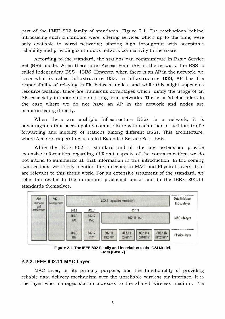
part of the IEEE 802 family of standards; Figure 2.1. The motivations behind introducing such a standard were: offering services which up to the time, were only available in wired networks; offering high throughput with acceptable reliability and providing continuous network connectivity to the users.

According to the standard, the stations can communicate in Basic Service Set (BSS) mode. When there is no Access Point (AP) in the network, the BSS is called Independent BSS – IBBS. However, when there is an AP in the network, we have what is called Infrastructure BSS. In Infrastructure BSS, AP has the responsibility of relaying traffic between nodes, and while this might appear as resource-wasting, there are numerous advantages which justify the usage of an AP, especially in more stable and long-term networks. The term Ad-Hoc refers to the case where we do not have an AP in the network and nodes are communicating directly.

When there are multiple Infrastructure BSSs in a network, it is advantageous that access points communicate with each other to facilitate traffic forwarding and mobility of stations among different BSSs. This architecture, where APs are cooperating, is called Extended Service Set – ESS.

While the IEEE 802.11 standard and all the later extensions provide extensive information regarding different aspects of the communication, we do not intend to summarize all that information in this introduction. In the coming two sections, we briefly mention the concepts, in MAC and Physical layers, that are relevant to this thesis work. For an extensive treatment of the standard, we refer the reader to the numerous published books and to the IEEE 802.11 standards themselves.

Figure 2.1. The IEEE 802 Family and its relation to the OSI Model.

From [Gas02]

2.2.2. IEEE 802.11 MAC Layer

MAC layer, as its primary purpose, has the functionality of providing reliable data delivery mechanism over the unreliable wireless air interface. It is the layer who manages station accesses to the shared wireless medium. The

6

original standard utilizes Carrier Sense Medium Access with Collision Avoidance (CSMA/CA) as the access mechanism. This access method, however, wastes a significant percentage of channel capacity, but, it is a necessary feature to provide reliability in data transmission. Among many other features, it also supports Request-To-Sent (RTS) and Clear-To-Send (CTS) mechanisms to address the case when two nodes are not aware of the presence of each other and want to communicate with a node which in transmission range of both. RTS/CTS mechanism helps to avoid the corruption of the packets in the above scenario.

DCF

Distributed Coordination Function (DCF) is the basic 802.11 MAC layer. DCF uses the above-mentioned CSMA/CA method to share the medium between the stations. It may optionally use the RTS/CTS method as well. Under this method, collision rate is relatively high and there is no notion of Quality of Service (QoS) in the network.

PCF

Point Coordination Function (PCF) is another basic coordination function which is defined only in infrastructure mode, where stations are connected to an access point. AP is the element in control of access in the network and it uses two periods to enforce its policies. There is a Contention Period, in which, DCF method is used. The second period is the Contention Free Period, in which AP basically allows stations, by sending them a special authorization, to send packets.

IEEE 802.11e standard addressed the existing limitations in DCF and PCF. It particularly addressed the problem of QoS provisioning in the network by introducing a new coordination function: Hybrid Coordination Function – HCF.

EDCA – 802.11e

Enhanced DCF Channel Access (EDCA) is a method of channel access within the HCF. An EDCA is basically a QoS-enabled DCF. This is done by introducing the notion of traffic classes, by giving priority, in channel access, to real-time data, compared to delay-tolerant data.

HCCA – 802.11e

Corresponding to EDCA, HCF Controlled Channel Access (HCCA) is a QoS-enabled PCF. It also uses EDCA during the Contention Period. Stations transmit the information about their queues status and traffic classes to the AP and, based on this information, AP coordinates access to the medium between the stations.

7

2.2.3. IEEE 802.11 PHY Layer

IEEE 802.11 Physical layer is the interface between MAC layer and the air interface. The frame exchange between Physical layer and MAC is under the control of Physical Layer Convergence Procedure (PLCP). Physical Layer is the entity in charge of actual transmission using different modulation schemes over the air interface. It also informs the MAC layer about the activity status of medium.

Currently, there are four standards defining the physical layer: IEEE 802.11a, 802.11b, 802.11g and 802.11n. Among these, IEEE 802.11n is the newest which is still under standardization. It utilizes Multiple-input-multiple-output (MIMO) technology to achieve significantly higher rates.

All these Physical Layer standards define their operating frequency band, number of available channels and possible transmission rates. In this work, however, we only concentrate on IEEE 802.11a standard due its maturity and widespread deployment. IEEE 802.11a operates in 5 GHz band, uses 52-subcarrier Orthogonal Frequency-Division Multiplexing (OFDM) and specifies 8 available radio channels.

Further details of IEEE 802.11a physical layer standard are given within the different sections of this thesis.

2.3. The Importance of Knowing about Physical Layer

2.3.1. Introduction

In this section, we explore the importance and relevance of knowing about IEEE 802.11 Physical Layer from the point of view of Communication Researchers as well as point of view of Networking Researchers. Traditionally, Networking domain researchers did not pay so much attention to the concepts and phenomena related to physical layer, as the interaction between this layer and the layers that they were focused on, e.g., network layer, was not so significant in the context of wired networks. But, the interaction aspect has changed as wireless networks have gained significant importance. However, many Networking researchers have not grasped this paradigm shift yet. In the wireless domain, the most promising solutions now come from the experts who consider cross-layer issues, i.e., the interactions between layers in the network. In the following two sections, we briefly explore this matter.

2.3.2. Digital Communications Researchers

Digital communications researchers are naturally concerned with the issues related to Physical layer, be it in the context of wired networks, or in wireless

8

networks. Among different aspects of physical layer, concepts of large-scale path loss models as well as fading aspects, calculating Bit Error Rate at different stages of the communication system and bit error distributions within a packet, can be mentioned. After having mentioned these, it is obvious that communications researchers would be interested in working with a network simulator which takes into account all the relevant details of the physical layer.

2.3.3. Networking Researchers

Convincing networking researchers to take into account the physical layer issues, however, is not a trivial task. This reluctance among networking researchers regarding extending their work to physical layer might be attributed to the complexities involved in this layer. Also, they might not be really familiar with the concepts involved, or since working on wired networks did not necessitate having knowledge about physical layer, they now have to take the extra effort to polish that rusty know-how.

In this section, we base our argument, about the importance of knowing about physical layer by networking researchers, on the results reported by [TMB01].

As mentioned by the authors in [TMB01], the following factors in the physical layer are relevant to the performance evaluation of higher layer protocols:

- Signal Reception Method (BER-based or SNRT-based)

- Path Loss, Fading

- Interference and Noise Computation

- Physical preamble length

According to their findings, these factors affect absolute performance of a protocol as well as the relative ranking among protocols for the same scenario.

We, however, limit our argument by mentioning the part of their results that are relevant to this work, i.e., the effect of different propagation models: path loss and fading.

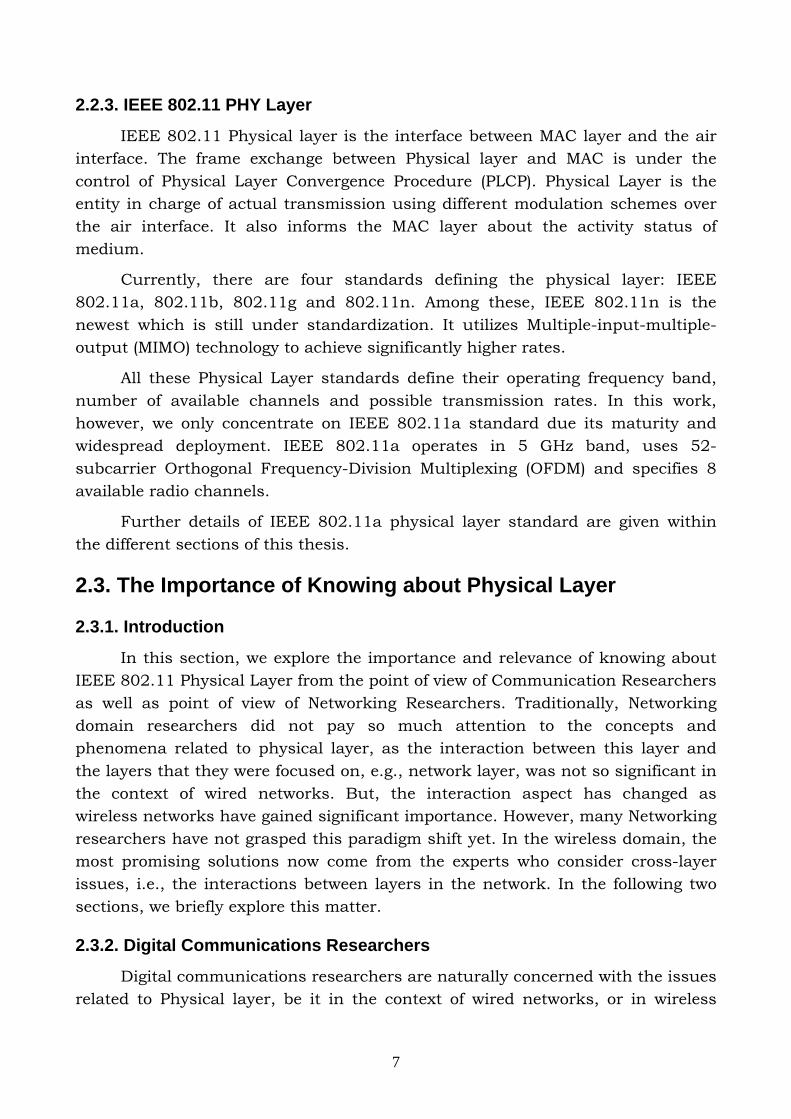
The chosen simulation scenario is as follows; 100 nodes with random waypoint mobility are considered moving in a flat square area with a side of 1200m. There are 40 Constant Bit Rate (CBR) sources in the network. The performance of two ad-hoc routing protocols are examined. These are: AODV (Ad-hoc On-demand Distance Vector) and DSR (Dynamic Source Routing). The metric that is chosen for this performance evaluation is Packet Delivery Ratio (PDR) which indicates the ratio of received packets to the sent ones. The result of the

9

evaluation is depicted in Figure 2.2. Please note that signal reception method is not under examination here, nevertheless, the same trend is evident in both cases of reception methods.

Figure 2.2. PDRs of AODV and DSR with different fading Models and two-ray path loss.

From [TMB01]

As suggested by the figure, AODV and DSR behave quite differently under increasingly harsh conditions. The performance of AODV deteriorates significantly as we go from no fading to Rayleigh fading. However, the performance of DSR proves to be much more consistent throughout, i.e., although it deteriorates, it’s not as severe as AODV’s case. The cause of this difference is in their route discovery processes due to link breaks as we move to the harsher fading types. The route discovery process in AODV has mush more overhead than that of DSR.

If a network researcher wants to compare the performance of these routing protocols, it is more likely that it does so by inspecting just the no-fading case. However, the reality of mobile ad-hoc networks is closer to Rayleigh or Rician type of fading. By looking at wrong part of the results due to being unfamiliar with propagation model concepts, a network researcher is more likely to arrive to wrong conclusions about the performance of routing protocols.

2.4. Introduction to YANS IEEE 802.11 Module

2.4.1. Introduction

This section briefly introduces the features of IEEE 802.11 module in YANS. Both MAC and Physical layers are treated. As MAC layer is not the focus of this work, we just briefly mention the available functionalities of existing MAC module. In the physical layer, however, we take a deeper look at the sequence of actions taken during the packet reception.

10

2.4.2. MAC

The MAC module implemented in YANS supports both ad-hoc mode and infrastructure mode. In ad-hoc mode, Distributed Coordination Function (DCF) is implemented along with the new QoS-enabled DCF in IEEE 802.11e, i.e., Enhanced DCF Channel Access (EDCA). In infrastructure mode, we have HCF (Hybrid Coordination Function) Controlled Channel Access (HCCA) implemented in the simulator.

In this work, however, we only use the ad-hoc mode since the emphasis of this thesis is on Physical layer issues. As explained later in detail, the simulation scenario chosen during the development of the physical layer and in Annex.2 is when two nodes are communicating in ad-hoc mode.

2.4.3. Details of PHY Layer Implementation in YANS

Propagation models, modulation and FEC coding schemes, BER and PER calculation methods are treated thoroughly in later chapters. In this section, we focus on the mechanics of the physical layer and enlighten the reader regarding the actions taken when a packet is received.

As YANS is an event-based simulator, for receiving each packet we have the following two events:

- An event at the start of reception (first bit of a packet)

- An event at the end of reception (last bit of a packet)

The SNIR(t) function is evaluated twice for each packet:

- For the first bit, for deciding whether or not the packet could be received, considering the current state of PHY and the SNIR(t) level.

- For the last bit, for calculating the final SNIR(t), considering what has happened during the packet reception, and for calculating the PER.

The PHY layer can be in one of four possible states:

- TX: the PHY is currently transmitting a signal. While the PHY is in this state, a received packet will be dropped regardless of its SNIR(t) level.

- SYNC: the PHY is synchronized on a signal and is waiting until it has received its last bit. While the PHY is in this state, another received packet will be dropped regardless of its SNIR(t) level. But, its signal level is recorded and taken into account in Noise Interference changes of the first packet on which the PHY was synchronized.

- BUSY: the PHY is not in the TX or SYNC, but the energy measured on the medium is higher than Energy Detection Threshold. While the PHY is in

11

this state, a packet can be received if its SNIR(t) level is above the threshold.

- IDLE: the PHY is not in the above states. The behavior is the same as BUSY state, i.e., while the PHY is in this state, a packet can be received if its SNIR(t) level is above the threshold.

The Steps Taken When the Last Bit of the Packet Is Received

When the last bit of the current packet, upon which the PHY is synchronized, is received, we again evaluate the SNIR(t) function and calculate the PER. Here are the details:

We remind that if any other packet was received during this time, i.e., from the first to the last bit of the current packet, all the received signal levels are recorded in the Noise Interference, Ni, vector and is taken into account for the current packet SNIR(t) calculation. If indeed, there was any other packet, i.e., the Ni vector has some elements, for each element of the vector, we calculate a Chunk Success Rate (CSR), taking into account the number of bits in that chunk, the respective SNIR(t) level in that chunk and the transmission mode (Modulation type, transmission rate, convolutional coding rate). The CSR calculation uses the theoretical BER formulas, based on modulation type, and also takes into account the convolutional code properties. It is in Chuck Success Rate calculation that we mention the desired type of error distribution within the packet. This process is then repeated for every Ni change recorded (since we have a different SNIR(t) value for each chunk, hence different BER and CSR). We multiply all these calculated CSRs to get the Packet Success Rate; hence the PER.

After having calculated the PER, we draw a random number from a uniform random number generator, between 0 and 1, and compare it against the PER. Whether the random number is higher than the PER or lower, we decide to mark the reception as correct, or as erroneous, respectively.

12

Chapter 3 – Large-scale Path Loss Models – Fading Channel

3.1. Introduction In this chapter, we explore both concepts of Large-scale Path Loss and

Fading. In Section 3.2, we introduce three models of Large-scale Path Loss which generally account for the large-scale attenuation of signal based on distance.

Section 3.3 introduces the Fading-related issues. Fading is the phenomenon responsible for rapid fluctuations of signal over a short period of time or distance. In reality, we can have only one channel, be it Large-scale Path Loss Channel, or Fading Channel. However, due to modeling constraints, we have chosen to separate what each of these two models represents, i.e., when we have only Large-scale Path Loss, then the channel can be chosen to act so, however, when we want to have Fading channel in the simulator, we need to use both models in cascade. The first part of the channel would be one of three Large-scale Path Loss Models and the second part of the channel would be the Fading channel. In this type of approach, Fading channel won’t have effect on the power of signal on average; it only introduces power fluctuations to the received signals. It is the Large-scale Path Loss model who accounts for the general attenuation of signal power based on distance.

13

3.2. Large-scale Path Loss Models

3.2.1. Introduction

This section introduces the classical large-scale path loss models. These models mostly address the effect of attenuation of signal based on distance. As will be presented hereafter, however, the level of sophistication and the inclusiveness of the models increase from the simple model of Free-space to the more realistic model of Shadowing.

3.2.2. Free-Space Model

Although a naïve model, Free-Space propagation model has been implemented as a choice for the path-loss model for comparison purposes. This model is used to predict the signal strength when the transmitter and the receiver have a clear, unobstructed line-of-sight path between them. Like other models, it predicts that received power decays as a function of Transmitter-Receiver distance raised to some power -typically to the second power. The well-known Friis equation, Equation 3.1, is used to calculate the received power:

(3.1)( ) Ld

GGPP rtt

r×××

= 2

2

4 πλ

Where, Pt is the transmitted power, Gt and Gr are transmitter antenna gain and that of receiver, respectively, d is the Transmitter-Receiver separation distance, L is the system loss -typically chosen as 1 and Lambda is the wavelength of the transmitted signal.

Of course, the Friis formula holds for values of d which are in the far-field region of the antenna, i.e., greater than [2 × (Largest physical linear dimension of the antenna) / λ]. Though it is not the case here, a more accurate approach would be to actually measure a reference power at a reference distance in the far-field region in any given wireless network, and then calculate the received power from the Friis formula using this reference power level for other distances. [Rap02]

3.2.3. Two-Ray Model

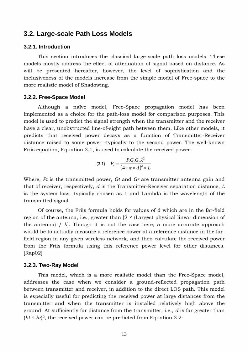
This model, which is a more realistic model than the Free-Space model, addresses the case when we consider a ground-reflected propagation path between transmitter and receiver, in addition to the direct LOS path. This model is especially useful for predicting the received power at large distances from the transmitter and when the transmitter is installed relatively high above the ground. At sufficiently far distance from the transmitter, i.e., d is far greater than (ht × hr)2, the received power can be predicted from Equation 3.2:

14

(3.2) ( )Ld

hhGGPP rtrtt

r 4

2

=

Where, ht is the height of transmitter, hr is the height of receiver and d is the T-R distance.

It is interesting to notice that at large values of d, the received power becomes independent of the frequency. Also, the received power attenuates much more rapidly with distance, compared to the Free-Space model, i.e., attenuates to the fourth power of the distance.[Rap02]

3.2.4. Shadowing Model

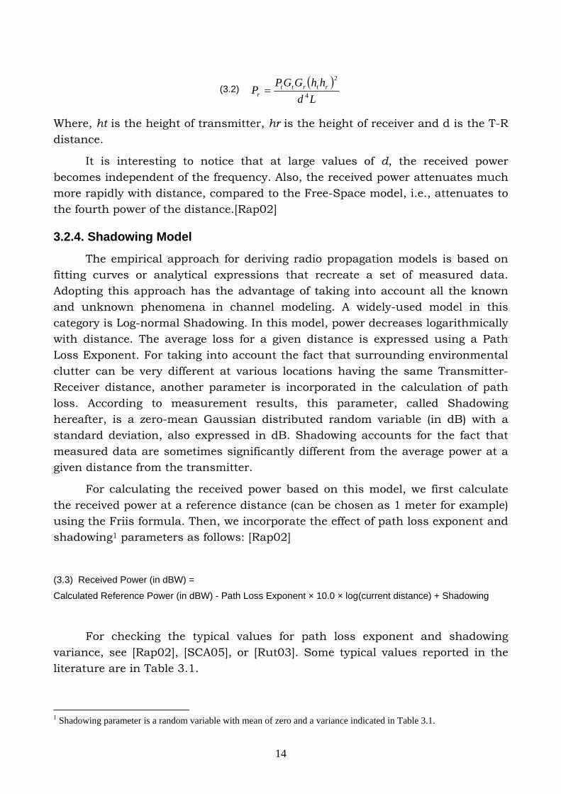
The empirical approach for deriving radio propagation models is based on fitting curves or analytical expressions that recreate a set of measured data. Adopting this approach has the advantage of taking into account all the known and unknown phenomena in channel modeling. A widely-used model in this category is Log-normal Shadowing. In this model, power decreases logarithmically with distance. The average loss for a given distance is expressed using a Path Loss Exponent. For taking into account the fact that surrounding environmental clutter can be very different at various locations having the same Transmitter-Receiver distance, another parameter is incorporated in the calculation of path loss. According to measurement results, this parameter, called Shadowing hereafter, is a zero-mean Gaussian distributed random variable (in dB) with a standard deviation, also expressed in dB. Shadowing accounts for the fact that measured data are sometimes significantly different from the average power at a given distance from the transmitter.

For calculating the received power based on this model, we first calculate the received power at a reference distance (can be chosen as 1 meter for example) using the Friis formula. Then, we incorporate the effect of path loss exponent and shadowing1 parameters as follows: [Rap02]

(3.3) Received Power (in dBW) =

Calculated Reference Power (in dBW) - Path Loss Exponent × 10.0 × log(current distance) + Shadowing

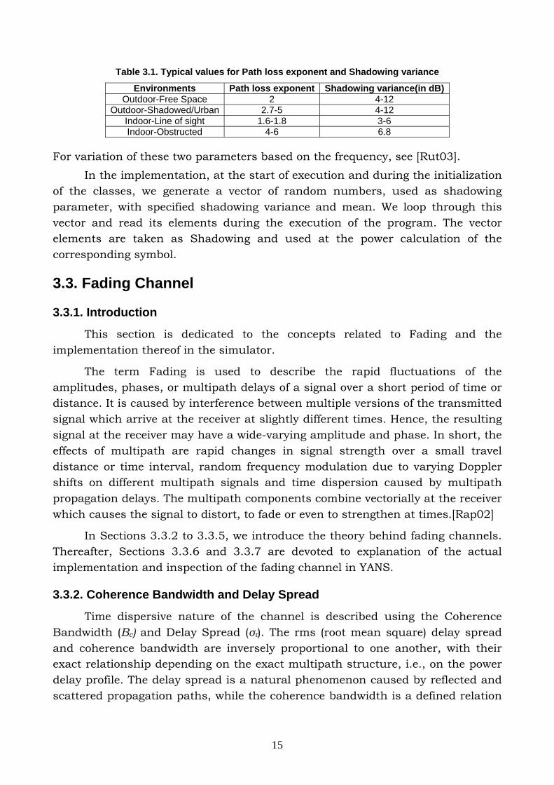
For checking the typical values for path loss exponent and shadowing variance, see [Rap02], [SCA05], or [Rut03]. Some typical values reported in the literature are in Table 3.1.

1 Shadowing parameter is a random variable with mean of zero and a variance indicated in Table 3.1.

15

Table 3.1. Typical values for Path loss exponent and Shadowing variance

Environments Path loss exponent Shadowing variance(in dB) Outdoor-Free Space 2 4-12

Outdoor-Shadowed/Urban 2.7-5 4-12 Indoor-Line of sight 1.6-1.8 3-6 Indoor-Obstructed 4-6 6.8

For variation of these two parameters based on the frequency, see [Rut03].

In the implementation, at the start of execution and during the initialization of the classes, we generate a vector of random numbers, used as shadowing parameter, with specified shadowing variance and mean. We loop through this vector and read its elements during the execution of the program. The vector elements are taken as Shadowing and used at the power calculation of the corresponding symbol.

3.3. Fading Channel

3.3.1. Introduction

This section is dedicated to the concepts related to Fading and the implementation thereof in the simulator.

The term Fading is used to describe the rapid fluctuations of the amplitudes, phases, or multipath delays of a signal over a short period of time or distance. It is caused by interference between multiple versions of the transmitted signal which arrive at the receiver at slightly different times. Hence, the resulting signal at the receiver may have a wide-varying amplitude and phase. In short, the effects of multipath are rapid changes in signal strength over a small travel distance or time interval, random frequency modulation due to varying Doppler shifts on different multipath signals and time dispersion caused by multipath propagation delays. The multipath components combine vectorially at the receiver which causes the signal to distort, to fade or even to strengthen at times.[Rap02]

In Sections 3.3.2 to 3.3.5, we introduce the theory behind fading channels. Thereafter, Sections 3.3.6 and 3.3.7 are devoted to explanation of the actual implementation and inspection of the fading channel in YANS.

3.3.2. Coherence Bandwidth and Delay Spread

Time dispersive nature of the channel is described using the Coherence Bandwidth (Bc) and Delay Spread (στ). The rms (root mean square) delay spread and coherence bandwidth are inversely proportional to one another, with their exact relationship depending on the exact multipath structure, i.e., on the power delay profile. The delay spread is a natural phenomenon caused by reflected and scattered propagation paths, while the coherence bandwidth is a defined relation

16

derived from the rms delay spread. Coherence bandwidth indicates the range of frequencies over which the channel can be considered as flat, i.e., all the frequency components of the signal undergo equal gain and linear phase. If the coherence bandwidth is defined as the bandwidth over which the frequency correlation function is above 0.9, then:

(3.4) (Bc) ~ 1/ (50 στ)

3.3.3. Coherence Time and Doppler Spread

Time varying nature of the channel, caused by relative motion between the transmitter and the receiver and by movement of objects, is described by Coherence Time and Doppler Spread. Doppler spread, BD, is a measure of the spectral broadening. Doppler spectrum can be measured by sending a single sinusoidal tone of frequency fc and viewing the received signal spectrum, which have components from fc – fd to fc + fd, with fd being the Doppler shift. Doppler shift depends on the relative velocity and angle of movements. Coherence time Tc is the time domain dual of Doppler spread and is widely chosen as 0.423 / fm, with fm being the maximum Doppler shift given by (Velocity / λ).

If the Doppler spread (BD) is far smaller than the baseband signal bandwidth (here, the 22 MHz channel bandwidth of 802.11), or alternatively, if the coherence time of the channel is greater than the symbol transmission period, then, the channel is considered as a slow fading channel.

Typical values for coherence bandwidth, rms delay spread and Doppler spread are reported for IEEE 802.11 networks in [Mfl04] and [MLC05].

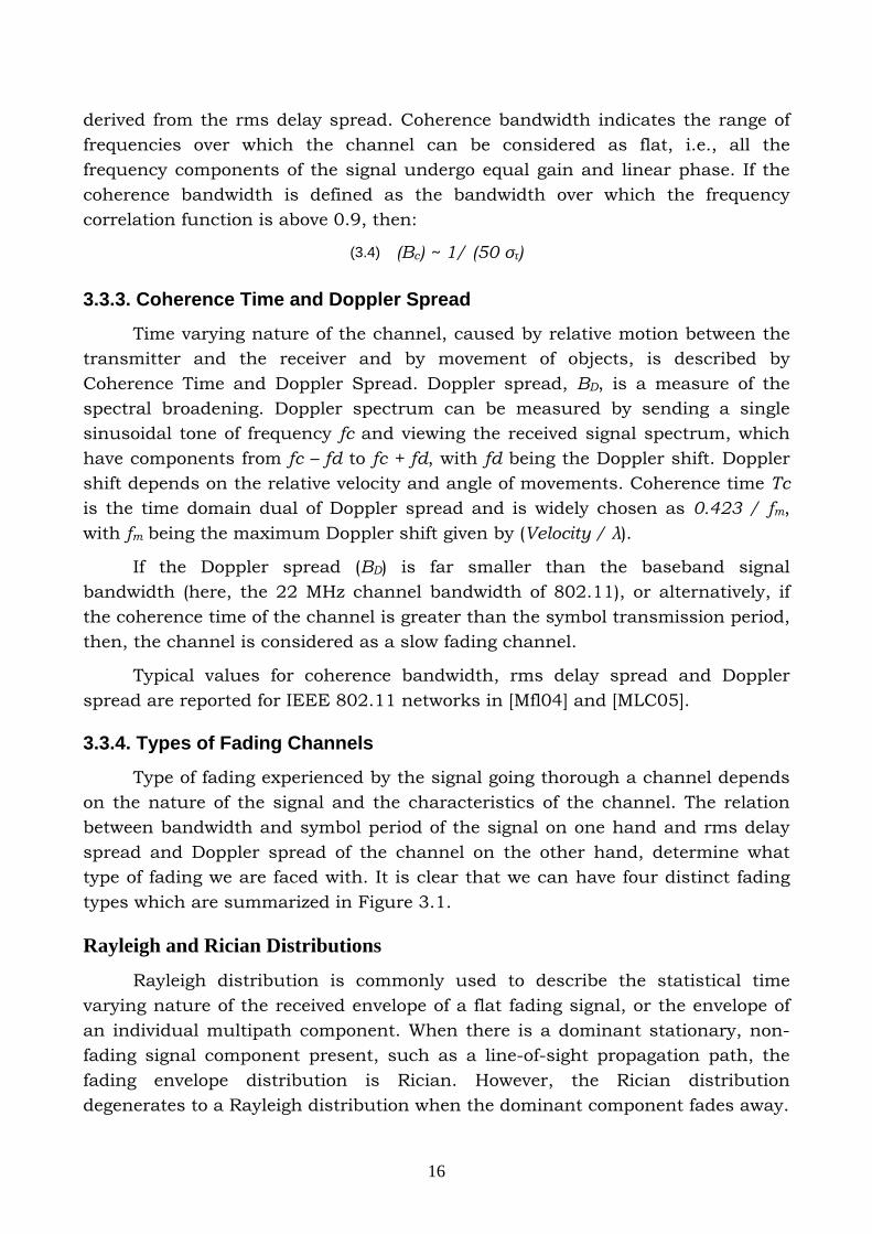
3.3.4. Types of Fading Channels

Type of fading experienced by the signal going thorough a channel depends on the nature of the signal and the characteristics of the channel. The relation between bandwidth and symbol period of the signal on one hand and rms delay spread and Doppler spread of the channel on the other hand, determine what type of fading we are faced with. It is clear that we can have four distinct fading types which are summarized in Figure 3.1.

Rayleigh and Rician Distributions

Rayleigh distribution is commonly used to describe the statistical time varying nature of the received envelope of a flat fading signal, or the envelope of an individual multipath component. When there is a dominant stationary, non-fading signal component present, such as a line-of-sight propagation path, the fading envelope distribution is Rician. However, the Rician distribution degenerates to a Rayleigh distribution when the dominant component fades away.

17

Figure 3.1. Cases of small-scale fading. From [Rap02]

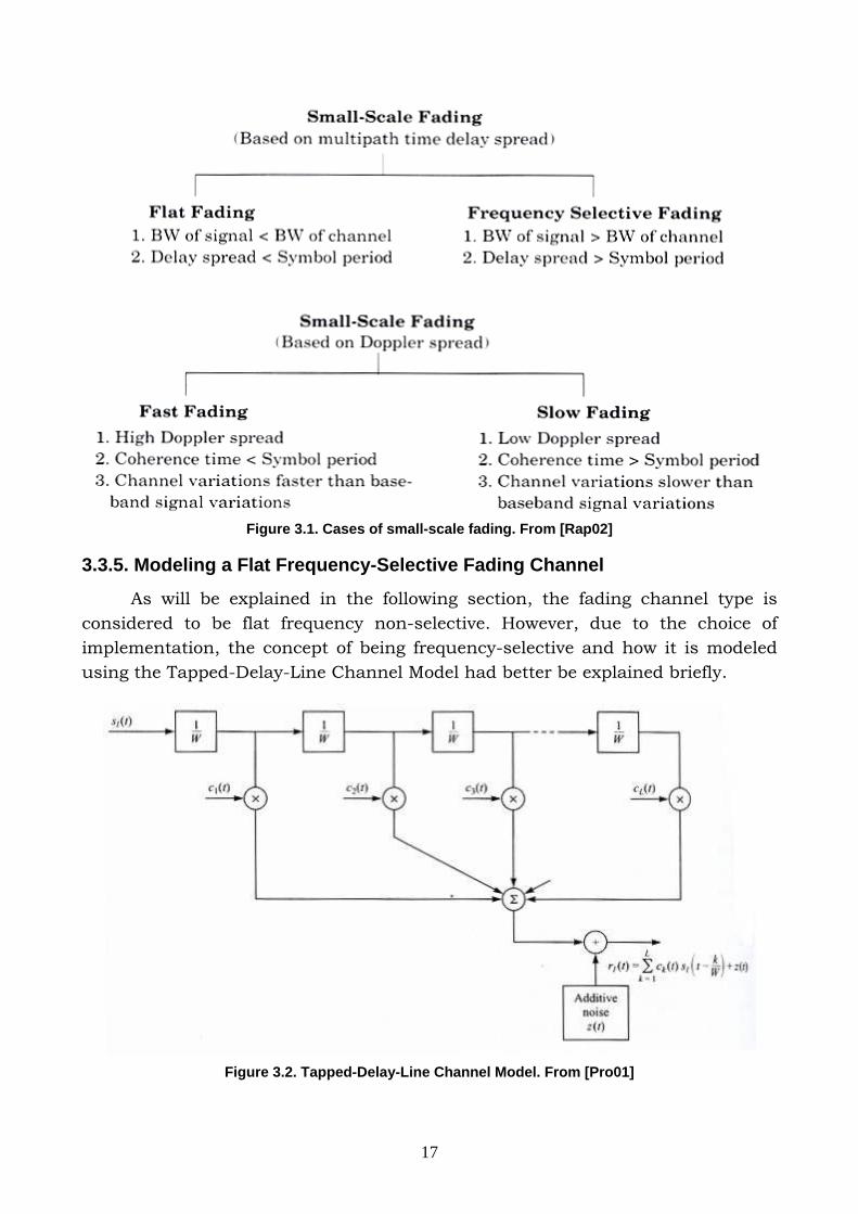
3.3.5. Modeling a Flat Frequency-Selective Fading Channel

As will be explained in the following section, the fading channel type is considered to be flat frequency non-selective. However, due to the choice of implementation, the concept of being frequency-selective and how it is modeled using the Tapped-Delay-Line Channel Model had better be explained briefly.

Figure 3.2. Tapped-Delay-Line Channel Model. From [Pro01]

18

If we consider the bandwidth of the transmitted signal as W, after the derivations detailed in [Pro01], we can show that the low-pass impulse response for the channel is:

(3.5) ( ) )()(;1 W

ntctcL

nn −= ∑

=

τδτ

Where, Tm is the total multipath spread, L is a practical number of considered taps which is equal to [Tm W] +1.

Note that we see a resolution of 1/W in the multipath delay profile and in the special case of Rayleigh fading, the magnitudes of the tap weights, |Cn(t)|, are Rayleigh distributed.

In the coming sections, we will see that we can set Channel Profiles for our chosen channel, by setting the number of taps, different powers (weights) associated to each tap and the delay experienced by each tap.

3.3.6. The Selected Fading Type Implemented in YANS

The current implementation in YANS, models a slow flat fading channel, i.e., the channel is neither frequency-selective, nor of fast fading type. According to the results reported in [MFl04], each Wi-Fi channel bandwidth is not larger than the coherence bandwidth, so, considering the channel frequency non-selective, seems to be a safe assumption. Also, the channel does not experience any changes during the transmission of each symbol, i.e., channel's coherence time is bigger than transmission time of each symbol. This latter assumption is again logical, especially in the context of indoor 802.11, where we do not have extremely fast movements in the environment.

Implementation

IT++ library has been chosen for the implementation of the fading channel among other libraries. IT++ is a C++ library of mathematical, signal processing, speech processing, and communications classes and functions. It is being developed by researchers in these areas and is widely used by researchers, both in the communications industry and universities.[IT06]

The implementation of the Communication Channels in IT++ is mostly based on the methods, algorithms and Matlab files provided in [Pat02].

If the user wants to consider the fading case, he needs to choose one of the large-scale path loss channel models as the first half of the model and the fading channel as the second half. The implementation of fading channel is very flexible and puts all the power of IT++ library at the user's disposal. The user may select a Rayleigh channel or a Rician one for simulating a slow flat fading channel.

19

At the start of the simulation, we generate FADING_NUMBER_OF_SAMPLES number of the fading process and store them in an IT++ data construct. However, before the generation of the fading process, we need to set a couple of parameters:

- NORMALIZED_DOPPLER_FREQUENCY

Which is the Doppler Frequency normalized by the Baud Rate of the transmission. Doppler Frequency itself can be derived by dividing SpeedOfObjects by Lambda of the transmission.

- Channel Profile

The average power effect of the fading process to the received signal power level, is set to 0 dB, since we already choose a large-scale path loss model as the first half of our channel model which accounts for this effect. We need to comply with the usage syntax of IT++, so we need to also set the delays in the taps for Tapped Delay Line modeling of frequency-selective channels. As we consider indoor 802.11 channel model as flat, we just consider one tap and set the delay to 0.

- Line-of-Sight parameter --Rician Model

Rician channel model is the default model for our fading channel, as it also degenerates to Rayleigh channel model by setting the LOS parameter to 0.

- SIMULATION_BAUD_RATE

This parameter is used to discretize Channel_Specification before assigning it to the channel (A requirement of IT++). This basically sets the unit of time for our channel and the set tap delays are treated considering this unit of time. The discretization should be set to transmitted signal period, i.e., to 1/(SIMULATION_BAUD_RATE/48). Signal here means the transmitted OFDM symbol. Each OFDM symbol has 48 data sub-carriers. If using BPSK modulation, each OFDM symbol will carry 48 bits of data. We also know that the maximum physical bit rate in IEEE 802.11a standard is 54 Mbits/s. Considering these matters, we realize the lowest unit of time concerning fading process can be set to 1/(54000000/48). We apply each element of the fading process to each transmitted OFDM symbol and in order to be able to do that, we always monitor the current Physical sending rate and the used modulation type.

After setting all these parameters, we can generate the fading process and use it during the simulation. In the default case, we always randomize the IT++'s random number generator in order to get a different fading process in each run of the simulation. After multiple runs of the simulation and averaging over the results, we can have simulation results which are more reliable, in statistical terms. However, the user may comment out the respective section to make his

20

results reproducible. During the execution of the program, we loop through the fading process matrix and upon reception of every symbol, we take an element as the fading factor and increase the position marker in the fading process.

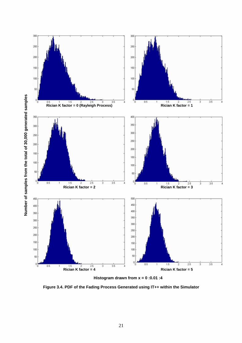
3.3.7. Examination of the Generated Fading Processes

After running a simulation in our simulator, the fading process is also saved on the disk for possible further inspections. We can load this file into Matlab to examine the process using the accompanying Matlab file, itload.m. We can examine the power (envelope) of the fading process by a Matlab command like “semilogy(abs(fading_process_coeffs(1:200)).^2)”. We call the power of the fading process at each sample as Fading Factor. The mean of the multiplicative fading power factor is nearly 1 and can be inspected by a Matlab command like “mean(abs(fading_process_coeffs).^2)”.

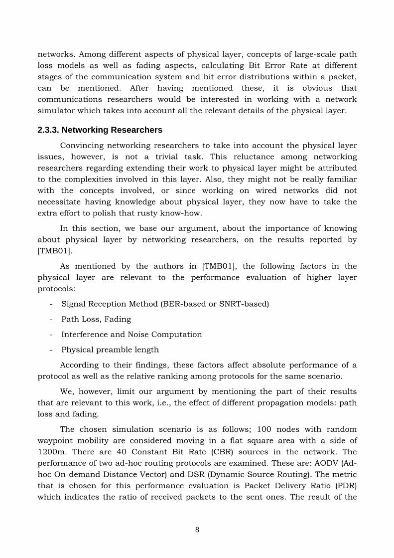
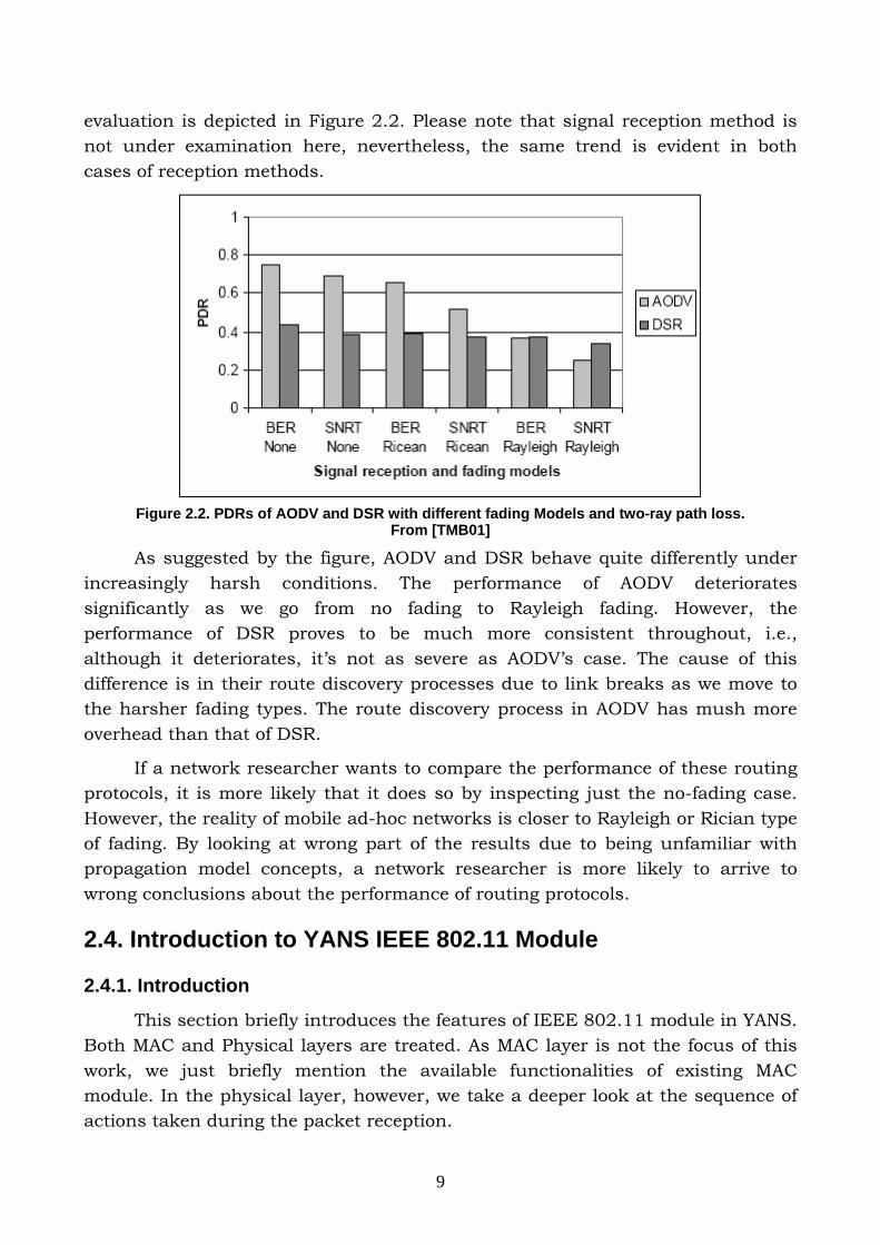
In Figure 3.3, the effect of selection of different Doppler frequencies is depicted. The PDF of the processes for different values of the Rician K factor are depicted in Figure 3.4 with the aid of the Matlab histogram function, “hist((abs(fading_process_coeffs(1:20000))), x)”.

Figure 3.3. Different Doppler Frequencies

21

Rician K factor = 0 (Rayleigh Process)

Rician K factor = 1

Rician K factor = 2

Rician K factor = 3

Num

ber o

f sam

ples

from

the

tota

l of 3

0,00

0 ge

nera

ted

sam

ples

Rician K factor = 4 Rician K factor = 5

Histogram drawn from x = 0 :0.01 :4

Figure 3.4. PDF of the Fading Process Generated using IT++ within the Simulator

22

Chapter 4 – Modulation Schemes and FEC Details

4.1. Introduction In this chapter, the details of convolutional encoder/decoder, i.e., the

Forward Error Correction (FEC) mechanism, and the modulation schemes existing in the IEEE 802.11a standard are provided. In the first section, the concept of convolutional coding of data bits, coding rates and related issues are presented. In the second section, different modulation schemes used for different transmission rates are mentioned. At last, a table summarizing all the available features is given for reference.

4.2. Convolutional Encoder–Decoder In this section, the terminology of convolution encoding and decoding is

presented, along with some figures depicting some of the concepts involved. The encoding and decoding suggested in IEEE 802.11a standard are also explained.

4.2.1. Encoding

The number of bits that are fed into the encoder at once is usually denoted by k and is called the input frame. n denotes the number of bits coming out of encoder at once and is called the output frame. Memory Constraint Length, v, denotes the total number of shift registers in the encoder and K, denotes the Input Constraint Length which is the total number of bits involved in the

23

encoding operation. K is hence equal to v+k. The coding rate is also defined as k/n. In the encoder of IEEE 802.11a standard, the encoder has an input constraint length of 7, 1 input bit (k) and 2 output bits (n). Hence, the basic coding rate is ½. Higher rates are achieved from this basic rate by employing puncturing that is a process through which some of encoded bits in the transmitter are omitted and in place of them, some dummy zeros are fed into the Viterbi decoder at the receiver side. This has the effect of reducing the number of transmitted bits and hence, increasing the coding rate. Through puncturing, the coding rate of 2/3 and 3/4 can be achieved according to IEEE 802.11a standard.

The encoding operation can be described by polynomials; one polynomial for representing each output bit, from each input bit. A simple convolutional encoder is depicted in Figure 4.1. Each block in this figure represents a shift register and is denoted as D in the generator polynomial, i.e., a single frame delay. For the case of the encoder depicted in this figure, we can write the polynomial equations as in Equation set 4.1.

Figure 4.1. A Simple Convolutional Encoder. From [Swe02]

1)( 2)1( ++= DDDg(4.1)

1)( 2)0( += DDg [Swe02]

These generator polynomials can be seen to correspond to the encoder depicted in Figure 4.1. Generator polynomials are usually represented in octal format. So in the case of the encoder in Figure 4.1, the first polynomial can be represented as 7, and the second as 5.

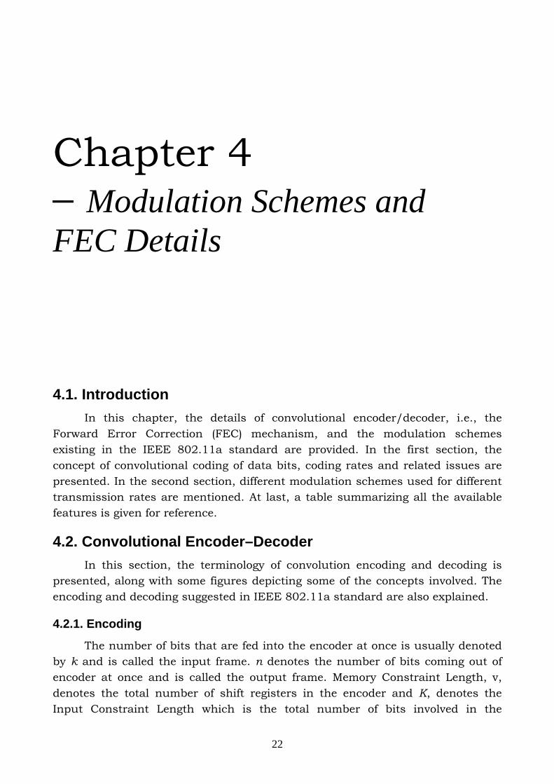
Convolutional code is a special case of a larger family of codes called tree codes. If a tree code has finite constraint length and is linear, it is a convolutional code. If an encoder has v shift register stages, then the contents of those shift registers can take 2v states. The encoder states can be represented in diagrammatic form with arcs to show allowed transitions and the associated input and output frames. The state diagram of the encoder depicted in Figure 4.1, is shown in Figure 4.2.

24

Figure 4.2. Encoder State Diagram. From [Swe02]

The states are labeled according to the contents of the encoder memory and input bit and output bits, due to that input bit, are indicated on the transitions.

Concepts of distance determine the error correcting properties of the code. Because of linearity, we can assess the distance properties of the code relative to the all-zero sequence. Free Path is the code path which leaves the zero state and returns to it some time later and in the process it produces a minimum number of 1s on the output. By looking at the state diagram, it can be discovered that we have minimum Hamming weight of 5 for the path connecting states 00-01-10-00 which results the output frames 11 10 11. This minimum weight is called the free distance of the code.

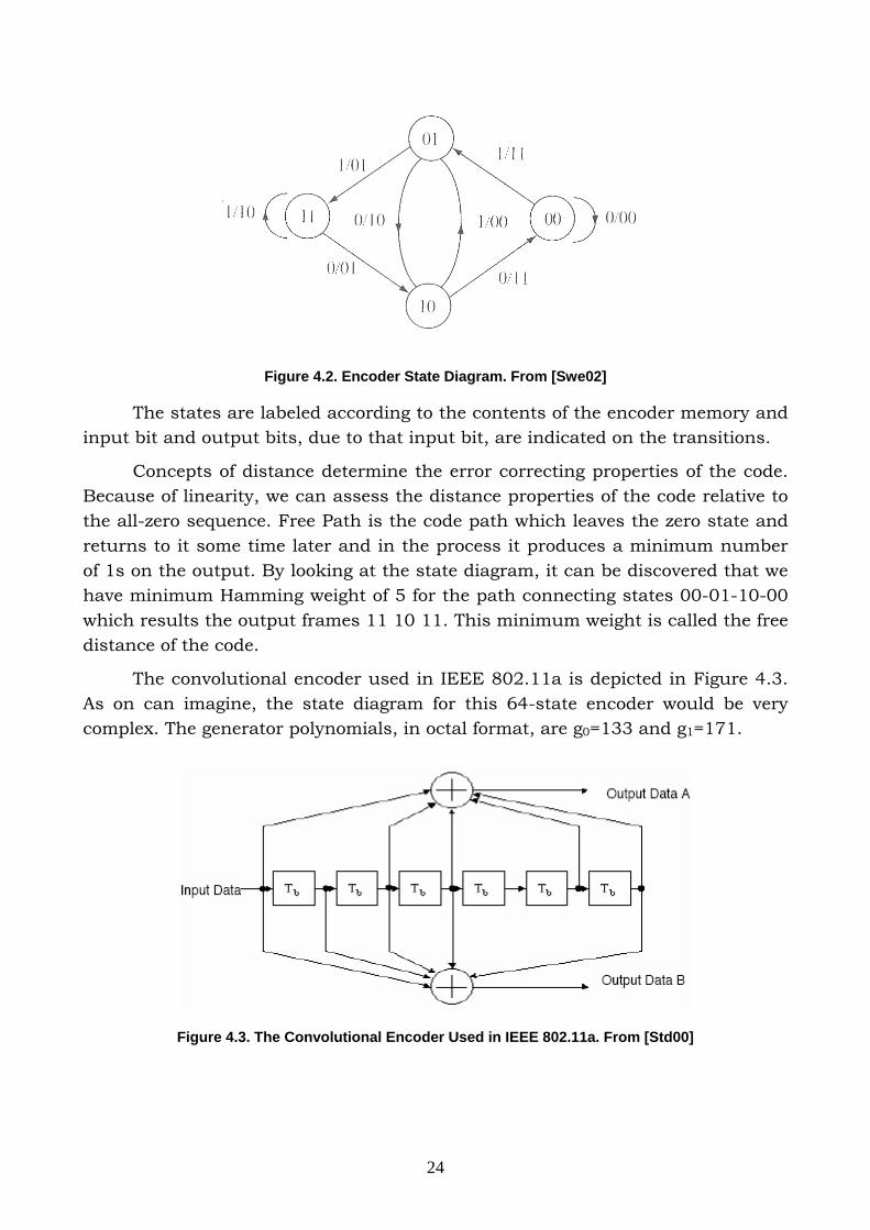
The convolutional encoder used in IEEE 802.11a is depicted in Figure 4.3. As on can imagine, the state diagram for this 64-state encoder would be very complex. The generator polynomials, in octal format, are g0=133 and g1=171.

Figure 4.3. The Convolutional Encoder Used in IEEE 802.11a. From [Std00]

25

4.2.2. Viterbi Decoding

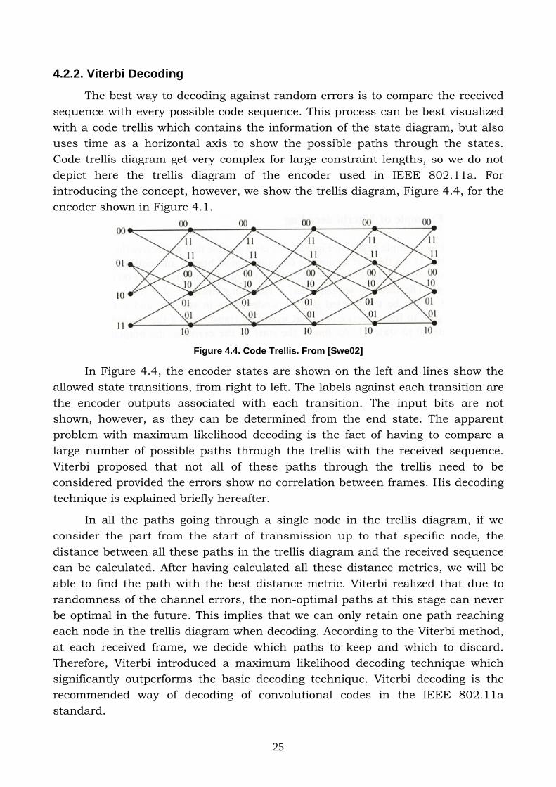
The best way to decoding against random errors is to compare the received sequence with every possible code sequence. This process can be best visualized with a code trellis which contains the information of the state diagram, but also uses time as a horizontal axis to show the possible paths through the states. Code trellis diagram get very complex for large constraint lengths, so we do not depict here the trellis diagram of the encoder used in IEEE 802.11a. For introducing the concept, however, we show the trellis diagram, Figure 4.4, for the encoder shown in Figure 4.1.

Figure 4.4. Code Trellis. From [Swe02]

In Figure 4.4, the encoder states are shown on the left and lines show the allowed state transitions, from right to left. The labels against each transition are the encoder outputs associated with each transition. The input bits are not shown, however, as they can be determined from the end state. The apparent problem with maximum likelihood decoding is the fact of having to compare a large number of possible paths through the trellis with the received sequence. Viterbi proposed that not all of these paths through the trellis need to be considered provided the errors show no correlation between frames. His decoding technique is explained briefly hereafter.

In all the paths going through a single node in the trellis diagram, if we consider the part from the start of transmission up to that specific node, the distance between all these paths in the trellis diagram and the received sequence can be calculated. After having calculated all these distance metrics, we will be able to find the path with the best distance metric. Viterbi realized that due to randomness of the channel errors, the non-optimal paths at this stage can never be optimal in the future. This implies that we can only retain one path reaching each node in the trellis diagram when decoding. According to the Viterbi method, at each received frame, we decide which paths to keep and which to discard. Therefore, Viterbi introduced a maximum likelihood decoding technique which significantly outperforms the basic decoding technique. Viterbi decoding is the recommended way of decoding of convolutional codes in the IEEE 802.11a standard.

26

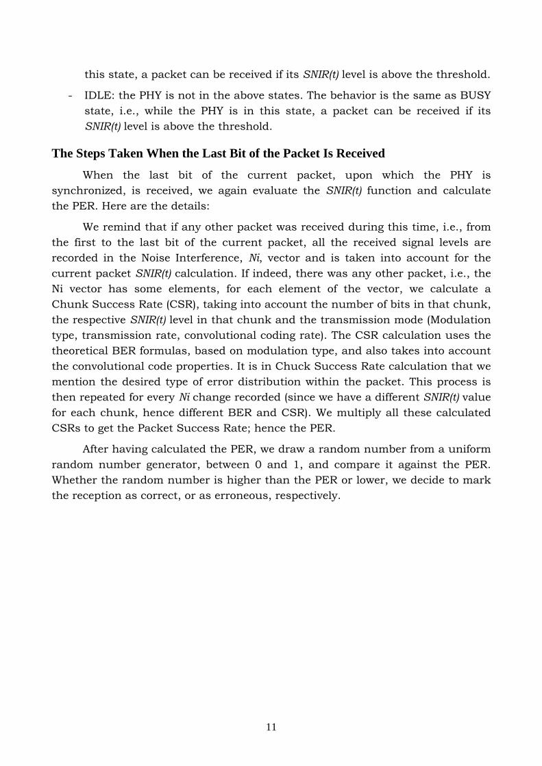
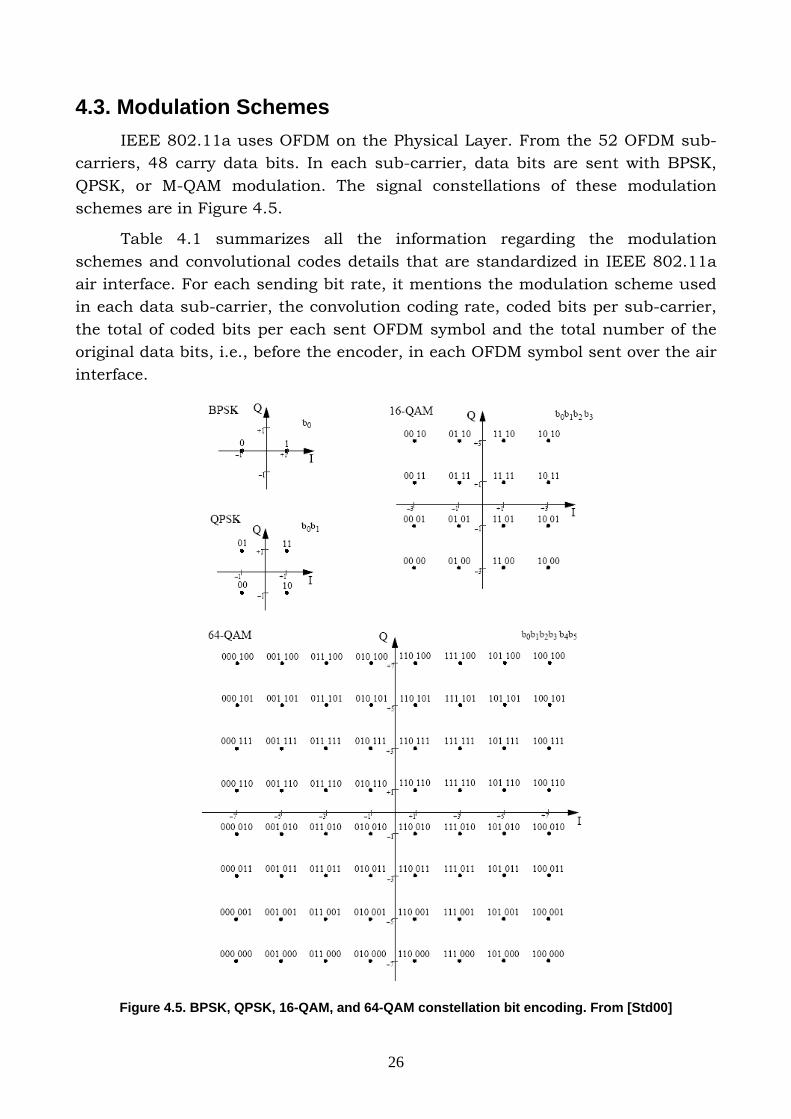
4.3. Modulation Schemes IEEE 802.11a uses OFDM on the Physical Layer. From the 52 OFDM sub-

carriers, 48 carry data bits. In each sub-carrier, data bits are sent with BPSK, QPSK, or M-QAM modulation. The signal constellations of these modulation schemes are in Figure 4.5.

Table 4.1 summarizes all the information regarding the modulation schemes and convolutional codes details that are standardized in IEEE 802.11a air interface. For each sending bit rate, it mentions the modulation scheme used in each data sub-carrier, the convolution coding rate, coded bits per sub-carrier, the total of coded bits per each sent OFDM symbol and the total number of the original data bits, i.e., before the encoder, in each OFDM symbol sent over the air interface.

Figure 4.5. BPSK, QPSK, 16-QAM, and 64-QAM constellation bit encoding. From [Std00]

27

Table 4.1. Rate-dependant parameters. Modulation and Coding Schemes. From [Std00]

28

Chapter 5 – Bit Error Rate, Packet Error Rate and Error Masks

5.1. Introduction This chapter is dedicated to the concepts and implementations of Bit and

Packet Error Rate calculations and Error Masks generation.

In section 5.2, different cases of BER calculation after the demodulator are presented by mentioning the respective formulas. We then go on to introduce the method and the involved formulas of BER calculation after the Viterbi decoder.

Section 5.3 introduces the two methods of Packet Error Rate calculation and the manner with which we can generate error masks in each case. Error masks are at bit level, so the user would be able to map these masks to applications packets at the application layer to test their behavior in view of the erroneous received bits.

5.2. BER Before and After Decoder

5.2.1. Introduction

In this section, we introduce the Bit Error Rate (BER) calculation methods. The BER calculation after demodulator, and before the Viterbi decoder, depends on the type of modulation and the channel type. Due to error correction mechanisms of the convolutional codes, the BER before the decoder is not the

29

same as the BER after the decoder. For deriving the latter, we need to have knowledge about the used convolutional code. The first section is dedicated to introducing the methods used to derive the BER before the Viterbi decoder, and after the demodulator, and the second section treats the BER calculation methods after the Viterbi decoder.

5.2.2. BER After Modulator – Before Decoder

In every chuck in the packet, where Ni and Signal level are constant, we calculate the Eb/N0 from Equation 5.1:

(5.1) ),(

),(),(0 tkR

BtkSNIRtk

NE

b

tb =

Where Eb is energy per bit, N0 is the noise power density, Bt is the bandwidth of the signal (20 MHz in 802.11a) and Rb(k,t) is the bit rate of transmission for packet k at time t.

The following BER formulas, depending on the channel and modulation types, are implemented and can be chosen in phy-80211.h with the following directive:

#define TYPE_OF_CHANNEL_FOR_BER

The Q function, the Error Function, erf(), and the Complementary Error Function, erfc(), are used in the following formulas. Here are the basic definitions and relations:

(5.2) ∫∞ −

=u

dttuQπ2

)2/exp()(2

[ZPe01, Equ.4.16]

The relation between Q function and erfc function; the latter exists in math.h:

(5.3) )2

(5.0)( xerfcxQ ×= [ZPe01, Equ.E.7]

The relationship between )(0N

ESNR b

bb ==γ and )(0N

ESNR s

ss ==γ and between

Ps (Symbol Error Probability or Rate) and Pb (Bit Error Probability or Rate):

bM

s SNRSNR ×= 2log(5.4)

bM

s PP ×= 2log [Gol05, Equs.6.2-3]

The above approximate conversions typically assume that the symbol energy is divided equally among all bits, and that Gray encoding is used so that at reasonable SNRs, one symbol error corresponds to exactly one bit error. In the simulator, based on the sent rate, we consider the used modulation according to

30

Table 5.1.

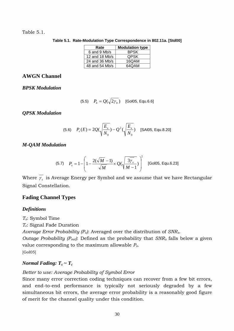
Table 5.1. Rate-Modulation Type Correspondence in 802.11a. [Std00]

Rate Modulation type6 and 9 Mb/s BPSK

12 and 18 Mb/s QPSK 24 and 36 Mb/s 16QAM 48 and 54 Mb/s 64QAM

AWGN Channel

BPSK Modulation

(5.5) )2( bb QP γ= [Gol05, Equ.6.6]

QPSK Modulation

(5.6) )()(2)(0

2

0 NE

QNE

QEP sss −= [SAl05, Equ.8.20]

M-QAM Modulation

(5.7)

2

)1

3()1(211

⎟⎟

⎠

⎞

⎜⎜

⎝

⎛

−×

−−−=

MQ

MMP s

sγ

[Gol05, Equ.6.23]

Where sγ is Average Energy per Symbol and we assume that we have Rectangular

Signal Constellation.

Fading Channel Types

Definitions

Ts: Symbol Time Tc: Signal Fade Duration Average Error Probability (Ps): Averaged over the distribution of SNRs. Outage Probability (Pout): Defined as the probability that SNRs falls below a given value corresponding to the maximum allowable Ps. [Gol05]

Normal Fading: Ts ~ Tc

Better to use: Average Probability of Symbol Error Since many error correction coding techniques can recover from a few bit errors, and end-to-end performance is typically not seriously degraded by a few simultaneous bit errors, the average error probability is a reasonably good figure of merit for the channel quality under this condition.

31

Slow Fading: Ts << Tc

Better to use: Outage Probability A deep fade will affect many simultaneous symbols. Thus, fading may lead to large error bursts, which cannot be corrected for with coding of reasonable complexity. Therefore, these error bursts can seriously degrade end-to-end performance. In this case acceptable performance cannot be guaranteed over all time or, equivalently, throughout a cell, without drastically increasing transmission power. Under these circumstances, an outage probability is specified so that the channel is deemed unusable for some fraction of time or space. This type of Fading Channel is more relevant to Indoor 802.11 Networks.

Fast Fading: Tc << Ts

Better to use: BER for AWGN channel Fading will be averaged out by the matched filter in the demodulator. Thus, performance is the same as in AWGN.

Slow-Fading Channel

cs TT <<

The Outage Probability, Pout, is:

(5.8) sePoutγγ /01 −−= [Gol05, Equ.6.47]

Pout is independent of modulation type.

Fading Channel

cs TT ~ : Normal Fading

BPSK Modulation

(5.9) ]1

1[21

b

bbP

γγ+

−= [Gol05, Equ.6.58]

QPSK Modulation

(5.10) )]/tan(1[tan11

1111 1

, MM

P Rays πααπα

++

++

−−= − [ZPe01, Equ.5.44]

Where, RaysP , is average symbol error probability for Rayleigh fading, M is 4 for

QPSK and )]/(sin/[1 2

0

MNEs πα = .

32

M-QAM Modulation

(5.11) ]5.01

5.01[

2 sM

sMMsP

γβγβα

+−= [Gol05, Equ.6.61]

Where M

MM

)1(4 −=α and

13−

=MMβ for Rectangular M-QAM.

Fast-Fading Channel

sc TT <<

The BER is calculated like the AWGN case.

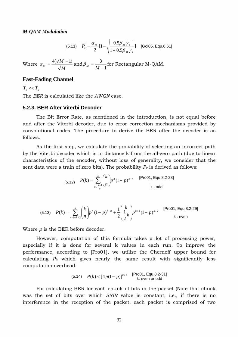
5.2.3. BER After Viterbi Decoder

The Bit Error Rate, as mentioned in the introduction, is not equal before and after the Viterbi decoder, due to error correction mechanisms provided by convolutional codes. The procedure to derive the BER after the decoder is as follows.

As the first step, we calculate the probability of selecting an incorrect path by the Viterbi decoder which is in distance k from the all-zero path (due to linear characteristics of the encoder, without loss of generality, we consider that the sent data were a train of zero bits). The probability Pk is derived as follows:

(5.12) ∑+

=

−−⎟⎟⎠

⎞⎜⎜⎝

⎛=

k

kn

nkn ppnk

kP

21

)1()( [Pro01, Equ.8.2-28]

k : odd

(5.13) 2/2/

2/1

)1(21

21)1()( kk

k

kn

nkn ppkk

ppnk

kP −⎟⎟

⎠

⎞

⎜⎜

⎝

⎛+−⎟⎟

⎠

⎞⎜⎜⎝

⎛= ∑

+=

−[Pro01, Equ.8.2-29]

k : even

Where p is the BER before decoder.

However, computation of this formula takes a lot of processing power, especially if it is done for several k values in each run. To improve the performance, according to [Pro01], we utilize the Chernoff upper bound for calculating Pk which gives nearly the same result with significantly less computation overhead:

(5.14) 2/)]1(4[)( kppkP −< [Pro01, Equ.8.2-31]k: even or odd

For calculating BER for each chunk of bits in the packet (Note that chuck was the set of bits over which SNIR value is constant, i.e., if there is no interference in the reception of the packet, each packet is comprised of two

33

chunks; one for Physical layer header, or PLCP header, and one for the Physical layer payload), we calculate the first 10 elements of Pk, multiply each by the corresponding Ck1 value and sum over the result of multiplications. This sum is the BER after decoder for the bits in the given chuck. Here is the formula to calculate BER from Ck and Pk values:

(5.15) ∑∞

=

<freedk

kk PCPunc

BER 1 [Vit71, Equ.20] [FOO98, Equ.3.6]

Punc, in the above formula, is the puncturing period of the convolutional code. Typical values of free distance(dfree) and cd for various convolutional codes are mentioned in a study documented in [FOO98].

5.3. PER Calculation Methods and Error Masks

5.3.1. Introduction

In this section, we introduce the two implemented methods for Packet Error Rate (PER) calculation. The first method is the simple Uniform Error Distribution, and the second one, is a new method presented in [KSa06].

5.3.2. Uniform Error Distribution

In every chuck in a packet (a chunk of n bits), where Ni (Noise Interference) and Signal level are constant, we calculate the Chunk Success Rate (CSR) according to Equation 5.16.

(5.16) nbitsBERCSR )1( −=

To get the PER, we multiply all the calculated CSRs in the packet to get the overall Packet Success Rate, hence the PER. This method of PER calculation makes the assumption that bit errors are uniformly distributed within the packet.

Error Mask Generation

To get the Mask Errors in the case of uniform error distribution, we simply draw a random number between 0 and 1 and compare the number against the BER that we have calculated for the given chunk. Depending on whether the random number is bigger than the BER or smaller, we write 0 or 1, respectively, on the disk. We repeat this process n times to produce n mask bits when we have n bits in the chunk.

1 Ck is the bit error number associated with each error event of distance k

34

5.3.3. Non-Uniform Error Distribution

In this section, a new error distribution is introduced which is presented in [KSa06]. The authors in that study argue that uniform error distribution leads to over-estimation of PER. They have carried out a theoretical work leading to new PER calculation formulas which are presented hereafter. Some notions are first presented along with their formulas.

Error Event Rate, Equation 5.17, is a probability indicating the frequency of occurred error events in any chunk which depends on the current SNR and the convolutional code details.

(5.17) freedSNRRdfreeeAEER ..≈ [KSa06]

According to the paper, each decoding epoch is comprised of an errorless period followed by an error event. Errorless period has mean length of W and its length follows a geometric distribution with parameter λ, which in turn can be calculated, according to Equation 5.18, using the EER, current SNR and convolution code details.

(5.18) EERrrSNRSNRn

v

EERw

ccc

])..2

2(

1)1[(1

1

+−++−

==λ [KSa06]

Where nc is the number of output bits, v is the memory constraint length and rc is the rate of the convolutional encoder.

The probability that a packet contains an error event is simply given by the probability that the errorless period begins at the first bit of the packet and lasts less than the packet length N. This is going to be the CDF of the geometric distribution with parameter λ, as given in Equation 5.19.

(5.19) NPER )1(1 λ−−= [KSa06]

Error Mask Generation

The error mask generation in this case of non-uniform error distribution is also done differently, compared to uniform error distribution. In the generated error masks, we will have mostly 0s, as errorless zones, with sporadic error events, marked by series of mostly 1s. The algorithm to generate the masks is as follows.

We first generate a random number from an exponential distribution with its parameter set as EER. Using a modulo calculation, we make sure that the number is smaller than our chunk size. We take this number as the end bit of the

35

first error event in the chunk. We draw another random number from an exponential distribution with parameter 1/τ, where τ is average error event length, as given in Equation 5.20.

(5.20) )..2

2(

1)1(ccc rrSNRSNRn

v+−

++=τ[KSa06]

This second random number indicates the length of the first error event in the chunk. Now, we have both the exact position and length of the first error event in the chunk. For the number of bits in this error period, we draw a random number, between 0 and 1, and compare it to BER/EER. If the random number is bigger, we write 0, otherwise, we write 1. For all the errorless periods in the chunk, we write 0s as the error masks. We can also consider that multiple error events can happen within each chunk. In this case, we can repeat the procedure and if the first generated random number, which indicated the end bit of the error event, shows a position between the first error event and the last bit of the chuck, we accept this as another error event in the chunk and proceed to generate error masks based on the mentioned procedure. In the current implementation in the simulator, we consider that multiple error events can happen and the implementation is therefore a bit complex.

36

Chapter 6 – Concluding Remarks & Future Work

6.1. Concluding Remarks In this thesis, we first explained the motivation behind this work, i.e.,

modeling a feature-rich IEEE 802.11a. Afterwards, in various chapters, we explained different building blocks of an IEEE 802.11a physical layer. Where interesting and worthwhile, we mentioned the implementation choices made during the development of the module, considering YANS original architecture.

As mentioned before, there is a long way towards having a realistic IEEE 802.11 simulation. This is not only due to complexities involved in the implementation of the current features, but also due to the host of unknown phenomena surrounding physical layer, including different characteristics of the wireless cards of various manufacturers. In this work, we have tried to model major known features of the physical layer within the simulator which, most probably, shortens the gap between simulation results and actual experimentations.

6.2. Emulab and ORBIT For validation of our models, the only option would be turning to

measurement-based approaches. Currently, there are two well-known, publicly-

37

accessible IEEE 802.11 testbeds: Emulab and ORBIT.

These two testbeds, although both are IEEE 802.11 testbeds, have major differences. ORBIT is a testbed installed in a clutter-less indoor environment. Although, at first sight, it does not seem to be a good choice for validating an IEEE 802.11 model, especially at physical layer, it is certainly a good starting point due to more predictable achieved results. These results could ultimately be used as configuring the basic simulator parameters. Emulab, however, is a fully-fledged wireless network, installed in a university campus. Due to its main functionality, which is basically providing wireless connectivity to the campus, it resembles, more closely, the realistic wireless environment. However, this feature is not just a benefit, but also introduces complexities in our measurement-based validation process, since depending on the chosen nodes in the network, completely different, or even contradictory, experimentation results could be produced.

6.3. Future Work As implied in the previous section, we emphasize that there is no such a

thing as one best IEEE 802.11 physical layer configuration. In the experiments, depending on the environment in which the network has been installed and parameters of the wireless cards of various manufacturers, for the same scenario, different measurement results could be produced. In light of this matter, an IEEE 802.11 simulator has zero chance of producing simulation results which correlate with measurement results, without pre-feeding it with information about the simulated environment.

However, there is still a point that is worth considering. It is the ability of producing simulation results, which are in correlation with experimentation results, when the simulator is pre-configured with the information about the environment in which the actual network has been installed. We could call such a simulator as human-aided cognitive simulator.

As our future work, we intend to explore this possibility by running the same scenario in the simulator and in the mentioned testbeds. It is of high value to see that if it is possible to configure the simulator to produce outputs which are in meaningful correlation with the outputs produced by experimentations. If that is possible, then we can safely declare that the level of details, and accuracy, of our IEEE 802.11 models are at satisfactory level.

38

Annex.1. A Brief Overview of Fading Channel Implementation in NS-2

The design and implementation of fading channel in YANS has been inspired by the fading channel implemented in NS-2. However, the implementation in YANS is far more flexible. As elaborated in the following sections, the implementation of fading channel in YANS is clearer, in terms of its capabilities and limitations and, we believe, has avoided the probable mistakes of the NS-2’s implementation.

A.1.1. Implementation in NS-2 A pre-calculated fading process has been saved in a text file and distributed

in their package. This text file is first read into an array in memory. Depending on the maximum velocity of surrounding objects, which is set in the TCL script of the simulation scenario, the Doppler frequency(fm) is calculated. The pre-calculated fading process has taken into account the maximum Doppler frequency (fm0) of 30 Hz. Then, the ratio of fm/fm0 is calculated. This ratio is multiplied by the current time; the time the signal is being received and the received power being calculated. Result of this multiplication is proportional to the index value of the fading process array stored in the memory. So, the smaller the fm/fm0 ratio, the slower the forward-move is in the array of fading process, i.e., if the ratio is very small, the same samples will be read over and over from the fading process array, before increasing the array index.

In Figure A.1.1, the fading process's power is depicted for the process generated statically for NS2 and a typical generation of IT++. Obviously, this is

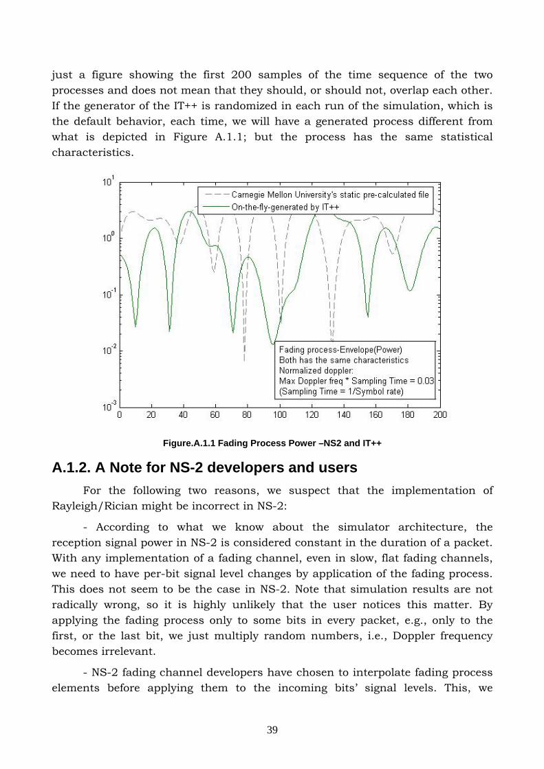
39

just a figure showing the first 200 samples of the time sequence of the two processes and does not mean that they should, or should not, overlap each other. If the generator of the IT++ is randomized in each run of the simulation, which is the default behavior, each time, we will have a generated process different from what is depicted in Figure A.1.1; but the process has the same statistical characteristics.

Figure.A.1.1 Fading Process Power –NS2 and IT++

A.1.2. A Note for NS-2 developers and users For the following two reasons, we suspect that the implementation of

Rayleigh/Rician might be incorrect in NS-2:

- According to what we know about the simulator architecture, the reception signal power in NS-2 is considered constant in the duration of a packet. With any implementation of a fading channel, even in slow, flat fading channels, we need to have per-bit signal level changes by application of the fading process. This does not seem to be the case in NS-2. Note that simulation results are not radically wrong, so it is highly unlikely that the user notices this matter. By applying the fading process only to some bits in every packet, e.g., only to the first, or the last bit, we just multiply random numbers, i.e., Doppler frequency becomes irrelevant.

- NS-2 fading channel developers have chosen to interpolate fading process elements before applying them to the incoming bits’ signal levels. This, we

40

suspect, just smoothes out the fading process, i.e., implicitly decreases the chosen Doppler frequency, and hence, might not be correct.

* We emphasize that these observations might not be as worrisome as we presume, but are definitely worth explaining in their documentation, if indeed the implementation is correct.

41

Annex.2. A Simple Simulation Scenario: 2 Nodes Communicating in Ad-hoc Mode

A.2.1. Code “main-80211-adhoc.cc” /* -*- Mode:C++; c-basic-offset:8; tab-width:8; indent-tabs-mode:t -*- */ /* * Copyright (c) 2005,2006 INRIA * All rights reserved. * * This program is free software; you can redistribute it and/or modify * it under the terms of the GNU General Public License version 2 as * published by the Free Software Foundation; * * This program is distributed in the hope that it will be useful, * but WITHOUT ANY WARRANTY; without even the implied warranty of * MERCHANTABILITY or FITNESS FOR A PARTICULAR PURPOSE. See the * GNU General Public License for more details. * * You should have received a copy of the GNU General Public License * along with this program; if not, write to the Free Software * Foundation, Inc., 59 Temple Place, Suite 330, Boston, * MA 02111-1307 USA * * Authors: * Masood Khosroshahy <m.kh@ieee.org> * Mathieu Lacage <mathieu.lacage@sophia.inria.fr> */ #include "yans/host.h" #include "yans/network-interface-80211.h" #include "yans/network-interface-80211-factory.h" #include "yans/channel-80211.h" #include "yans/ipv4-route.h" #include "yans/simulator.h" #include "yans/udp-source.h" #include "yans/udp-sink.h" #include "yans/periodic-generator.h" #include "yans/traffic-analyser.h" #include "yans/callback.h" #include "yans/pcap-writer.h" #include "yans/trace-container.h"

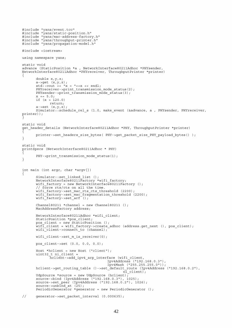
42

#include "yans/event.tcc" #include "yans/static-position.h" #include "yans/mac-address-factory.h" #include "yans/throughput-printer.h" #include "yans/propagation-model.h" #include <iostream> using namespace yans; static void advance (StaticPosition *a , NetworkInterface80211Adhoc *PHYsender, NetworkInterface80211Adhoc *PHYreceiver, ThroughputPrinter *printer) { double x,y,z; a->get (x,y,z); std::cout << "x = "<<x << endl; PHYreceiver->print_transmission_mode_status(2); PHYsender->print_transmission_mode_status(3); x += 5.0; if (x > 120.0) return; a->set (x,y,z); Simulator::schedule_rel_s (1.0, make_event (&advance, a , PHYsender, PHYreceiver, printer)); } static void get_header_details (NetworkInterface80211Adhoc *PHY, ThroughputPrinter *printer) { printer->set_headers_size_bytes( PHY->get_packet_size_PHY_payload_bytes() ); } static void printSpecs (NetworkInterface80211Adhoc * PHY) { PHY->print_transmission_mode_status(1); } int main (int argc, char *argv[]) { Simulator::set_linked_list (); NetworkInterface80211Factory *wifi_factory; wifi_factory = new NetworkInterface80211Factory (); // force rts/cts on all the time. wifi_factory->set_mac_rts_cts_threshold (2200); wifi_factory->set_mac_fragmentation_threshold (2200); wifi_factory->set_arf (); Channel80211 *channel = new Channel80211 (); MacAddressFactory address; NetworkInterface80211Adhoc *wifi_client; StaticPosition *pos_client; pos_client = new StaticPosition (); wifi_client = wifi_factory->create_adhoc (address.get_next (), pos_client); wifi_client->connect_to (channel); wifi_client->set_m_is_receiver(0); pos_client->set (0.0, 0.0, 0.0); Host *hclient = new Host ("client"); uint32_t ni_client = hclient->add_ipv4_arp_interface (wifi_client, Ipv4Address ("192.168.0.3"), Ipv4Mask ("255.255.255.0")); hclient->get_routing_table ()->set_default_route (Ipv4Address ("192.168.0.2"), ni_client); UdpSource *source = new UdpSource (hclient); source->bind (Ipv4Address ("192.168.0.3"), 1025); source->set_peer (Ipv4Address ("192.168.0.2"), 1026); source->unbind_at (25); PeriodicGenerator *generator = new PeriodicGenerator (); // generator->set_packet_interval (0.000635);

43

// generator->set_packet_size (2000); //application payload in bytes generator->set_packet_interval (0.0000246); generator->set_packet_size (16); //application payload in bytes generator->start_now (); generator->stop_at (25); generator->set_send_callback (make_callback (&UdpSource::send, source)); ThroughputPrinter *printer = new ThroughputPrinter (); // printer->set_application_packet_interval (0.000635); // printer->set_application_packet_size (2000); //application payload in bytes printer->set_application_packet_interval (0.0000246); printer->set_application_packet_size (16); //application payload in bytes NetworkInterface80211Adhoc *wifi_server; StaticPosition *pos_server = new StaticPosition (); wifi_server = wifi_factory->create_adhoc (address.get_next (), pos_server); wifi_server->connect_to (channel); wifi_server->set_m_is_receiver(1); pos_server->set (5.0, 0.0, 0.0); Simulator::schedule_abs_s (0.5, make_event (&printSpecs, wifi_client)); Simulator::schedule_abs_s (0.5, make_event (&get_header_details, wifi_server, printer)); // Source is in wifi_client. In this scenario, receiver gradually moves further away. Simulator::schedule_abs_s (1.0, make_event (&advance, pos_server, wifi_client, wifi_server, printer)); Simulator::schedule_abs_s (25, make_event (&ThroughputPrinter::stop, printer)); Host *hserver = new Host ("server"); uint32_t ni_server = hserver->add_ipv4_arp_interface (wifi_server, Ipv4Address ("192.168.0.2"), Ipv4Mask ("255.255.255.0")); hserver->get_routing_table ()->set_default_route (Ipv4Address ("192.168.0.3"), ni_server); UdpSink *sink = new UdpSink (hserver); sink->bind (Ipv4Address ("192.168.0.2"), 1026); sink->unbind_at (25); /* run simulation */ Simulator::run (); /* destroy network */ delete wifi_client; delete wifi_server; delete wifi_factory; delete channel; delete source; delete generator; delete sink; delete printer; delete hclient; delete hserver; Simulator::destroy (); return 0; }

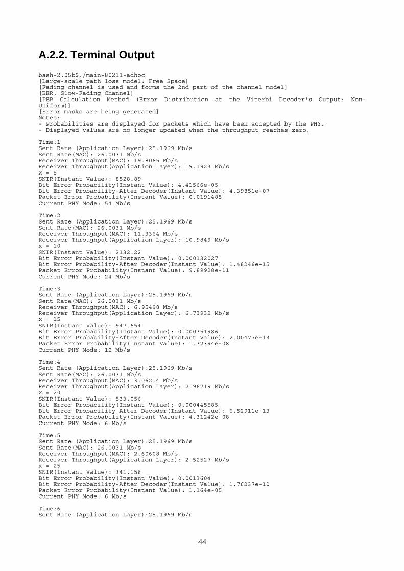
44

A.2.2. Terminal Output bash-2.05b$./main-80211-adhoc [Large-scale path loss model: Free Space] [Fading channel is used and forms the 2nd part of the channel model] [BER: Slow-Fading Channel] [PER Calculation Method (Error Distribution at the Viterbi Decoder's Output: Non-Uniform)] [Error masks are being generated] Notes: - Probabilities are displayed for packets which have been accepted by the PHY. - Displayed values are no longer updated when the throughput reaches zero. Time:1 Sent Rate (Application Layer):25.1969 Mb/s Sent Rate(MAC): 26.0031 Mb/s Receiver Throughput(MAC): 19.8065 Mb/s Receiver Throughput(Application Layer): 19.1923 Mb/s x = 5 SNIR(Instant Value): 8528.89 Bit Error Probability(Instant Value): 4.41566e-05 Bit Error Probability-After Decoder(Instant Value): 4.39851e-07 Packet Error Probability(Instant Value): 0.0191485 Current PHY Mode: 54 Mb/s Time:2 Sent Rate (Application Layer):25.1969 Mb/s Sent Rate(MAC): 26.0031 Mb/s Receiver Throughput(MAC): 11.3364 Mb/s Receiver Throughput(Application Layer): 10.9849 Mb/s x = 10 SNIR(Instant Value): 2132.22 Bit Error Probability(Instant Value): 0.000132027 Bit Error Probability-After Decoder(Instant Value): 1.48246e-15 Packet Error Probability(Instant Value): 9.89928e-11 Current PHY Mode: 24 Mb/s Time:3 Sent Rate (Application Layer):25.1969 Mb/s Sent Rate(MAC): 26.0031 Mb/s Receiver Throughput(MAC): 6.95498 Mb/s Receiver Throughput(Application Layer): 6.73932 Mb/s x = 15 SNIR(Instant Value): 947.654 Bit Error Probability(Instant Value): 0.000351986 Bit Error Probability-After Decoder(Instant Value): 2.00477e-13 Packet Error Probability(Instant Value): 1.32394e-08 Current PHY Mode: 12 Mb/s Time:4 Sent Rate (Application Layer):25.1969 Mb/s Sent Rate(MAC): 26.0031 Mb/s Receiver Throughput(MAC): 3.06214 Mb/s Receiver Throughput(Application Layer): 2.96719 Mb/s x = 20 SNIR(Instant Value): 533.056 Bit Error Probability(Instant Value): 0.000445585 Bit Error Probability-After Decoder(Instant Value): 6.52911e-13 Packet Error Probability(Instant Value): 4.31242e-08 Current PHY Mode: 6 Mb/s Time:5 Sent Rate (Application Layer):25.1969 Mb/s Sent Rate(MAC): 26.0031 Mb/s Receiver Throughput(MAC): 2.60608 Mb/s Receiver Throughput(Application Layer): 2.52527 Mb/s x = 25 SNIR(Instant Value): 341.156 Bit Error Probability(Instant Value): 0.0013604 Bit Error Probability-After Decoder(Instant Value): 1.76237e-10 Packet Error Probability(Instant Value): 1.164e-05 Current PHY Mode: 6 Mb/s Time:6 Sent Rate (Application Layer):25.1969 Mb/s

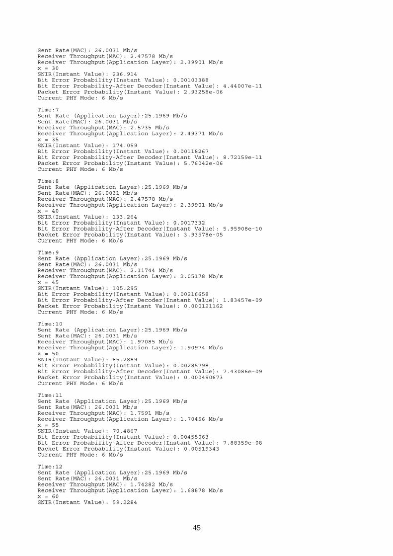
45

Sent Rate(MAC): 26.0031 Mb/s Receiver Throughput(MAC): 2.47578 Mb/s Receiver Throughput(Application Layer): 2.39901 Mb/s x = 30 SNIR(Instant Value): 236.914 Bit Error Probability(Instant Value): 0.00103388 Bit Error Probability-After Decoder(Instant Value): 4.44007e-11 Packet Error Probability(Instant Value): 2.93258e-06 Current PHY Mode: 6 Mb/s Time:7 Sent Rate (Application Layer):25.1969 Mb/s Sent Rate(MAC): 26.0031 Mb/s Receiver Throughput(MAC): 2.5735 Mb/s Receiver Throughput(Application Layer): 2.49371 Mb/s x = 35 SNIR(Instant Value): 174.059 Bit Error Probability(Instant Value): 0.00118267 Bit Error Probability-After Decoder(Instant Value): 8.72159e-11 Packet Error Probability(Instant Value): 5.76042e-06 Current PHY Mode: 6 Mb/s Time:8 Sent Rate (Application Layer):25.1969 Mb/s Sent Rate(MAC): 26.0031 Mb/s Receiver Throughput(MAC): 2.47578 Mb/s Receiver Throughput(Application Layer): 2.39901 Mb/s x = 40 SNIR(Instant Value): 133.264 Bit Error Probability(Instant Value): 0.0017332 Bit Error Probability-After Decoder(Instant Value): 5.95908e-10 Packet Error Probability(Instant Value): 3.93578e-05 Current PHY Mode: 6 Mb/s Time:9 Sent Rate (Application Layer):25.1969 Mb/s Sent Rate(MAC): 26.0031 Mb/s Receiver Throughput(MAC): 2.11744 Mb/s Receiver Throughput(Application Layer): 2.05178 Mb/s x = 45 SNIR(Instant Value): 105.295 Bit Error Probability(Instant Value): 0.00216658 Bit Error Probability-After Decoder(Instant Value): 1.83457e-09 Packet Error Probability(Instant Value): 0.000121162 Current PHY Mode: 6 Mb/s Time:10 Sent Rate (Application Layer):25.1969 Mb/s Sent Rate(MAC): 26.0031 Mb/s Receiver Throughput(MAC): 1.97085 Mb/s Receiver Throughput(Application Layer): 1.90974 Mb/s x = 50 SNIR(Instant Value): 85.2889 Bit Error Probability(Instant Value): 0.00285798 Bit Error Probability-After Decoder(Instant Value): 7.43086e-09 Packet Error Probability(Instant Value): 0.000490673 Current PHY Mode: 6 Mb/s Time:11 Sent Rate (Application Layer):25.1969 Mb/s Sent Rate(MAC): 26.0031 Mb/s Receiver Throughput(MAC): 1.7591 Mb/s Receiver Throughput(Application Layer): 1.70456 Mb/s x = 55 SNIR(Instant Value): 70.4867 Bit Error Probability(Instant Value): 0.00455063 Bit Error Probability-After Decoder(Instant Value): 7.88359e-08 Packet Error Probability(Instant Value): 0.00519343 Current PHY Mode: 6 Mb/s Time:12 Sent Rate (Application Layer):25.1969 Mb/s Sent Rate(MAC): 26.0031 Mb/s Receiver Throughput(MAC): 1.74282 Mb/s Receiver Throughput(Application Layer): 1.68878 Mb/s x = 60 SNIR(Instant Value): 59.2284

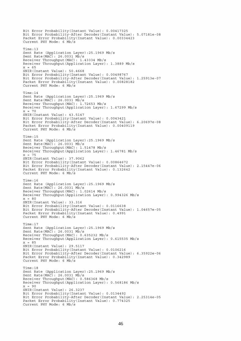
46

Bit Error Probability(Instant Value): 0.00417325 Bit Error Probability-After Decoder(Instant Value): 5.07181e-08 Packet Error Probability(Instant Value): 0.00334423 Current PHY Mode: 6 Mb/s Time:13 Sent Rate (Application Layer):25.1969 Mb/s Sent Rate(MAC): 26.0031 Mb/s Receiver Throughput(MAC): 1.43334 Mb/s Receiver Throughput(Application Layer): 1.3889 Mb/s x = 65 SNIR(Instant Value): 50.4668 Bit Error Probability(Instant Value): 0.00498767 Bit Error Probability-After Decoder(Instant Value): 1.25913e-07 Packet Error Probability(Instant Value): 0.00828182 Current PHY Mode: 6 Mb/s Time:14 Sent Rate (Application Layer):25.1969 Mb/s Sent Rate(MAC): 26.0031 Mb/s Receiver Throughput(MAC): 1.72653 Mb/s Receiver Throughput(Application Layer): 1.67299 Mb/s x = 70 SNIR(Instant Value): 43.5147 Bit Error Probability(Instant Value): 0.0043421 Bit Error Probability-After Decoder(Instant Value): 6.20697e-08 Packet Error Probability(Instant Value): 0.00409119 Current PHY Mode: 6 Mb/s Time:15 Sent Rate (Application Layer):25.1969 Mb/s Sent Rate(MAC): 26.0031 Mb/s Receiver Throughput(MAC): 1.51478 Mb/s Receiver Throughput(Application Layer): 1.46781 Mb/s x = 75 SNIR(Instant Value): 37.9062 Bit Error Probability(Instant Value): 0.00864672 Bit Error Probability-After Decoder(Instant Value): 2.15447e-06 Packet Error Probability(Instant Value): 0.132642 Current PHY Mode: 6 Mb/s Time:16 Sent Rate (Application Layer):25.1969 Mb/s Sent Rate(MAC): 26.0031 Mb/s Receiver Throughput(MAC): 1.02614 Mb/s Receiver Throughput(Application Layer): 0.994326 Mb/s x = 80 SNIR(Instant Value): 33.316 Bit Error Probability(Instant Value): 0.0116638 Bit Error Probability-After Decoder(Instant Value): 1.04657e-05 Packet Error Probability(Instant Value): 0.4991 Current PHY Mode: 6 Mb/s Time:17 Sent Rate (Application Layer):25.1969 Mb/s Sent Rate(MAC): 26.0031 Mb/s Receiver Throughput(MAC): 0.635232 Mb/s Receiver Throughput(Application Layer): 0.615535 Mb/s x = 85 SNIR(Instant Value): 29.5117 Bit Error Probability(Instant Value): 0.0106216 Bit Error Probability-After Decoder(Instant Value): 6.35922e-06 Packet Error Probability(Instant Value): 0.342989 Current PHY Mode: 6 Mb/s Time:18 Sent Rate (Application Layer):25.1969 Mb/s Sent Rate(MAC): 26.0031 Mb/s Receiver Throughput(MAC): 0.586368 Mb/s Receiver Throughput(Application Layer): 0.568186 Mb/s x = 90 SNIR(Instant Value): 26.3237 Bit Error Probability(Instant Value): 0.0134492 Bit Error Probability-After Decoder(Instant Value): 2.25314e-05 Packet Error Probability(Instant Value): 0.774325 Current PHY Mode: 6 Mb/s

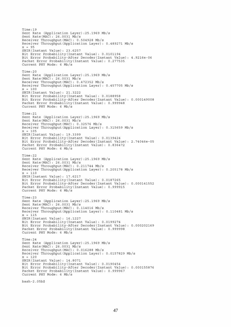
47

Time:19 Sent Rate (Application Layer):25.1969 Mb/s Sent Rate(MAC): 26.0031 Mb/s Receiver Throughput(MAC): 0.504928 Mb/s Receiver Throughput(Application Layer): 0.489271 Mb/s x = 95 SNIR(Instant Value): 23.6257 Bit Error Probability(Instant Value): 0.0101194 Bit Error Probability-After Decoder(Instant Value): 4.9216e-06 Packet Error Probability(Instant Value): 0.277535 Current PHY Mode: 6 Mb/s Time:20 Sent Rate (Application Layer):25.1969 Mb/s Sent Rate(MAC): 26.0031 Mb/s Receiver Throughput(MAC): 0.472352 Mb/s Receiver Throughput(Application Layer): 0.457705 Mb/s x = 100 SNIR(Instant Value): 21.3222 Bit Error Probability(Instant Value): 0.0188958 Bit Error Probability-After Decoder(Instant Value): 0.000149008 Packet Error Probability(Instant Value): 0.999948 Current PHY Mode: 6 Mb/s Time:21 Sent Rate (Application Layer):25.1969 Mb/s Sent Rate(MAC): 26.0031 Mb/s Receiver Throughput(MAC): 0.32576 Mb/s Receiver Throughput(Application Layer): 0.315659 Mb/s x = 105 SNIR(Instant Value): 19.3399 Bit Error Probability(Instant Value): 0.0139424 Bit Error Probability-After Decoder(Instant Value): 2.74046e-05 Packet Error Probability(Instant Value): 0.836472 Current PHY Mode: 6 Mb/s Time:22 Sent Rate (Application Layer):25.1969 Mb/s Sent Rate(MAC): 26.0031 Mb/s Receiver Throughput(MAC): 0.211744 Mb/s Receiver Throughput(Application Layer): 0.205178 Mb/s x = 110 SNIR(Instant Value): 17.6217 Bit Error Probability(Instant Value): 0.0187265 Bit Error Probability-After Decoder(Instant Value): 0.000141552 Packet Error Probability(Instant Value): 0.999915 Current PHY Mode: 6 Mb/s Time:23 Sent Rate (Application Layer):25.1969 Mb/s Sent Rate(MAC): 26.0031 Mb/s Receiver Throughput(MAC): 0.114016 Mb/s Receiver Throughput(Application Layer): 0.110481 Mb/s x = 115 SNIR(Instant Value): 16.1227 Bit Error Probability(Instant Value): 0.0199274 Bit Error Probability-After Decoder(Instant Value): 0.000202169 Packet Error Probability(Instant Value): 0.999998 Current PHY Mode: 6 Mb/s Time:24 Sent Rate (Application Layer):25.1969 Mb/s Sent Rate(MAC): 26.0031 Mb/s Receiver Throughput(MAC): 0.016288 Mb/s Receiver Throughput(Application Layer): 0.0157829 Mb/s x = 120 SNIR(Instant Value): 14.8071 Bit Error Probability(Instant Value): 0.0190454 Bit Error Probability-After Decoder(Instant Value): 0.000155876 Packet Error Probability(Instant Value): 0.999967 Current PHY Mode: 6 Mb/s bash-2.05b$

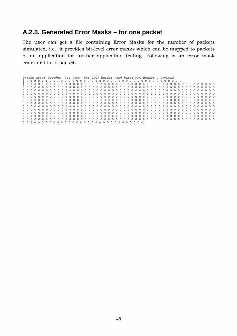
48

A.2.3. Generated Error Masks – for one packet The user can get a file containing Error Masks for the number of packets simulated, i.e., it provides bit-level error masks which can be mapped to packets of an application for further application testing. Following is an error mask generated for a packet: [Masks after decoder. 1st Part: PHY PLCP header -2nd Part: MAC Header & Payload | 0 0 0 0 0 1 0 1 1 0 0 0 0 0 0 0 0 0 0 0 0 0 0 0 0 0 0 0 0 0 0 0 0 0 0 0 0 0 0 0 0 | 0 0 0 0 1 0 1 1 0 0 0 0 0 0 0 0 0 0 0 0 0 0 0 0 0 0 0 0 0 0 0 0 0 0 0 0 0 0 0 0 0 0 0 0 0 0 0 0 0 0 0 0 0 0 0 0 0 0 0 0 0 0 0 0 0 0 0 0 0 0 0 0 0 0 0 0 0 0 0 0 0 0 0 0 0 0 0 0 0 0 0 0 0 0 0 0 0 0 0 0 0 0 0 0 0 0 0 0 0 0 0 0 0 0 0 0 0 0 0 0 0 0 0 0 0 0 0 0 0 0 0 0 0 0 0 0 0 0 0 0 0 0 0 0 0 0 0 0 0 0 0 0 0 0 0 0 0 0 0 0 0 0 0 0 0 0 0 0 0 0 0 0 0 0 0 0 0 0 0 0 0 0 0 0 0 0 0 0 0 0 0 0 0 0 0 0 0 0 0 0 0 0 0 0 0 0 0 0 0 0 0 0 0 0 0 0 0 0 0 0 0 0 0 0 0 0 0 0 0 0 0 0 0 0 0 0 0 0 0 0 0 0 0 0 0 0 0 0 0 0 0 0 0 0 0 0 0 0 0 0 0 0 0 0 0 0 0 0 0 0 0 0 0 0 0 0 0 0 0 0 0 0 0 0 0 0 0 0 0 0 0 0 0 0 0 0 0 0 0 0 0 0 0 0 0 0 0 0 0 0 0 0 0 0 0 0 0 0 0 0 0 0 0 0 0 0 0 0 0 0 0 0 0 0 0 0 0 0 0 0 0 0 0 0 0 0 0 0 0 0 0 0 0 0 0 0 0 0 0 0 0 0 0 0 0 0 0 0 0 0 0 0 0 0 0 0 0 0 0 0 0 0 0 0 0 0 0 0 0 0 0 0 0 0 0 0 0 0 0 0 0 0 0 0 0 0 0 0 0 0 0 0 0 0 0 0 0 0 0 0 0 0 0 0 0 0 0 0 0 0 0 0 0 0 0 0 0 0 0 0 0 0 0 0 0 0 0 0 0 0 0 0 0 0 0 0 0 0 0 0 0 0 0 0 0 0 0 0 0 0 0 0 0 0 0 0 0 0 0 0 0 0 0 0 0 0 0 0 0 0 0 0 0 0 0 0 0 0 0 0 0 0 0 0 0 0 0 0 0 0 0 0 0 0 0 0 0 0 0 0 0 0 0 0 0 0 0 0 0 0 0 0 0 0 0 0 0 0 0 0 0 0 0 0 0 0 0 0 0 0 0 0 0 0 0 0 0 0 0 0 0 0 0 0 0 0 0 0 0 0 0 0 0 0 0 0 0 0 0 0 0 0 0 0 0 0 0 0 0 0 0 0 0 0 0 0 0 0 0 0 0 0 0 0 0 0 0 0 0 0 0 0 0 0 0 0 0 0 0 0 0 0 0 0 0 0 0 0 0 0 0]

49

Annex.3. A Brief Comparative Study of IEEE 802.11 PHY-MAC Models in Well-known Open Source Network Simulators

In this study, we inspect the implementations of IEEE 802.11 PHY-MAC models of some of the high-profile, well-known, open-source network simulators. The simulators chosen are: NS2, OMNET++, GloMoSim, J-Sim, and YANS. The study concentrates on the availability and implementation flexibility of MAC modes and PHY propagation models. Furthermore, it is checked to see if the simulator produces packet error masks, in different simulation scenarios, for offline testing of the application behaviors. The type of license under which the code has been released is also mentioned.

50

A.3.1. NS2 Webpage: http://www.isi.edu/nsnam/ns/ Version: ns-2.30 released on Sept 26, 2006

A.3.1.1 MAC modes Ad-hoc: Supported Infrastructure: Supported

MAC modes-Original 802.11 MAC

Distributed Coordination Function (DCF)

Supported:

- A module is contributed by Carnegie Mellon University-CMU Monarch project in their ad-hockey extension to NS2 to simulate mobile nodes connected by wireless network interfaces, including the ability to simulate multi-hop wireless ad hoc networks. - Not distributed in the main package. - Ver.1.1.2 –11 August, 1999

Point Coordination Function (PCF)

Supported:

- A module is contributed by Anders Lindgren of Lulea University of Technology. - Not distributed in the main package. - Ver.0.8b –2001

MAC modes-802.11e MAC -Hybrid Coordination Function (HCF)

- A module is contributed by INRIA-Planete Group. Features: ET/SNRT/BER-based PHY models, 802.11a multirate and 802.11e HCCA and EDCA. This module has been improved further in the YANS project; among other improvements, non-occurrence of packet collisions has been fixed. - Not distributed in the main package. - Ver.14.2 –Sep 7, 2005

HCF Controlled Channel Access (HCCA):

Supported:

- A module contributed by Computer Netwoking Group at the University of Pisa. Their work allows for a flexible integration of different scheduling algorithms. A classifier tags incoming packets with the appropriate traffic stream identifier. The HCCA scheduler is used at both the QoS AP and QoS

51

stations. - Not distributed in the main package. - Ver.2006-08-23

Enhanced DCF Channel Access (EDCA):

Supported:

- A module is contributed by Telecommunication Networks Group of “Technische Universität Berlin”. Their work extends the wireless and mobility code, which has been developed in the CMU Monarch project. They have added the contention free bursting (CFB), or TXOP bursting, to their model, which allows the transmission of a train of small packets without intermediate contention. - Not distributed in the main package. - Ver.1.0 beta –Feb. 14, 2006

A.3.1.2. PHY Implemented Standard-Mode

- 802.11a –In the module contributed by INRIA-Planete Group - Not distributed in the main package. - Ver.14.2 –Sep 7, 2005

PHY propagation models

FreeSpace

Supported: The classical Friis formula is implemented –Based on the work of CMU Monarch project.

Two-Ray

Supported: The Two-Ray power reception calculation has been implemented. For close range, the FreeSpace model is used again –Contributed by CMU Monarch project.

Shadowing

Supported: The model is correctly implemented taking into account both Path Loss Exponent and Shadowing Variance. The work is done at USC/ISI.

Small-scale Fading

Supported: This model has been implemented by Antenna and Radio Communications Group of Carnegie Mellon University. The fading process has been computed once and saved in a text file, distributed in their package, according to an algorithm published by them in a paper. The implementation is explained in more detail in Annex 1. - Not distributed in the main package.

52

- Ver. Sep.2000

A.3.1.3. Packet Error Masks Not Supported

A.3.1.4. License

GPLv2 is the current license, but since the simulator has numerous contributors, the license of each specific module should be checked as a result. However, there is a specific exception added to GPLv2 which states that the module copyright holder gives the right that the model can be combined with free software programs or libraries that are released under the GNU LGPL license. Pre-existing software in the project are mostly governed by Original BSD license. Some new codes are under Apache 2.0 license. As recommended by NS2 developers, new code should use either GNU GPL, with the specific exception, or Modified BSD license, or Apache 2.0 license or Original BSD license.

53

A.3.2. OMNET++ Webpage: http://www.omnetpp.org/

The implementations are in three different projects which are based on the OMNET++ simulation framework: – INET Framework

Webpage: http://www.omnetpp.org/staticpages/index.php?page=20041019113420757 Version : 20061020

– Ipv6SuiteWithINET Webpage: http://ctieware.eng.monash.edu.au/twiki/bin/view/Simulation/IPv6Suite Version : 20060809

– Mobility Framework Webpage: http://mobility-fw.sourceforge.net/ Version : August 13, 2006

A.3.2.1. MAC modes

Ad-hoc: INET Framework: Supported Ipv6SuiteWithINET: Not Supported Mobility Framework: Supported

Infrastructure: INET Framework: Supported Ipv6SuiteWithINET: Supported Mobility Framework: Not Supported

MAC modes-Original 802.11 MAC

Distributed Coordination Function (DCF) INET Framework: Supported [CSMA/CA without RTS/CTS] Ipv6SuiteWithINET: Supported [But only functionalities for operating in Infrastructure mode] Mobility Framework: Supported [CSMA/CA with RTS/CTS]

Point Coordination Function (PCF) INET Framework: Supported Ipv6SuiteWithINET: Supported Mobility Framework: Not Supported

MAC modes-802.11e MAC -Hybrid Coordination Function (HCF)

HCF Controlled Channel Access (HCCA), Enhanced DCF Channel Access (EDCA) INET Framework: Not Supported Ipv6SuiteWithINET: Not Supported

54

Mobility Framework: Not Supported

A.3.2.2. PHY Implemented Standard-Mode 802.11b –In all three projects

PHY propagation models

FreeSpace Supported: The only implemented propagation model. Two-Ray,Shadowing,Small-scale Fading Not Supported

A.3.2.3. Packet Error Masks Not Supported

A.3.2.4. License

GPL for academic use Commercial License from SimulCraft for commercial use

55

A.3.3. GloMoSim Webpage: http://pcl.cs.ucla.edu/projects/glomosim/ Studied Version: Last release, 2.03-Dec 2000; before switching to the commercial product QualNet

A.3.3.1. MAC modes

Ad-hoc: Supported Infrastructure: Not Supported

MAC modes-Original 802.11 MAC

Distributed Coordination Function (DCF) Supported –CSMA/CA with RTS/CTS

Point Coordination Function (PCF) Not Supported

MAC modes-802.11e MAC -Hybrid Coordination Function (HCF)

HCF Controlled Channel Access (HCCA), Enhanced DCF Channel Access (EDCA) Not Supported

A.3.3.2. PHY Implemented Standard-Mode

Partial implementation of 802.11-1997: SNR bounded, BER based with BPSK/QPSK modulation

PHY propagation models

FreeSpace, Two-Ray: Supported: The implementation of these two propagation models is based on the description in T. S. Rappaport "Wireless Communications: Principles & Practice."

Shadowing Not Supported

Small-scale Fading Supported: Rician Fading has been implemented.

A.3.3.3. Packet Error Masks Not Supported

A.3.3.4. License

- Free for educational use (Access to download only granted to academic Top

56

Level Domains) Not covered by a standard well-known license. The user has the right to copy and modify the software at the condition that the resulting software is offered at no charge to research community. The original copyright notice should be included in any derivative work.

- Commercial license can also be obtained from UCLA. The development of GloMoSim has been discontinued. The product is now under active development under the name of the commercial product QualNet.

57

A.3.4. J-Sim Webpage: http://www.j-sim.org/ Version: 1.3 released on 2004/02/2; latest patch: 2006/05/07, patch 4.

A.3.4.1. MAC modes

Ad-hoc: Supported Infrastructure: Not Supported

MAC modes-Original 802.11 MAC

Distributed Coordination Function (DCF) Supported [CSMA/CA + RTS/CTS] –With implementation of Power Saving Mode

Point Coordination Function (PCF) Not Supported

MAC modes-802.11e MAC -Hybrid Coordination Function (HCF)

HCF Controlled Channel Access (HCCA), Enhanced DCF Channel Access (EDCA) Not Supported

A.3.4.2. PHY Implemented Standard-Mode

Implementation of few basic functionalities of the Physical Layer. Therefore, not adhering to any particular standard.

PHY propagation models

FreeSpace, Two-Ray Supported: The classical formulas are implemented.

Shadowing, Small-scale Fading: Not Supported

Another Implemented Model: Irregular Terrain Model Irregular Terrain Model, which is based on electromagnetic theory and on statistical analyses of both terrain features and radio measurements, predicts the median attenuation of a radio signal as a function of distance and the variability of the signal in time and in space. The model requires altitude on each point of the earth which can be obtained from Globe data that can be downloaded from a mentioned URL. When using Irregular Terrain Model, one must use ellipsoidal latitude and longitude coordinates instead of Cartesian coordinates.

A.3.4.3. Packet Error Masks Not Supported

A.3.4.4. License BSD

58

A.3.5. YANS Webpage: http://yans.inria.fr/ Version: Release 0.9.0 (2006-05-20) with ongoing improvements

A.3.5.1. MAC modes

Ad-hoc: Supported Infrastructure: Supported

MAC modes-Original 802.11 MAC

Distributed Coordination Function (DCF) Supported

Point Coordination Function (PCF) Not Supported

MAC modes-802.11e MAC -Hybrid Coordination Function (HCF)

HCF Controlled Channel Access (HCCA), Enhanced DCF Channel Access (EDCA) Supported

A.3.5.2. PHY Implemented Standard-Mode 802.11a

PHY propagation models

FreeSpace, Two-Ray Supported: The classical Friis formula, for FreeSpace model, and Two-Ray Ground Reflection formula, for Two-Ray model, have been implemented.

Shadowing Supported: A reference power, at a reference distance, is calculated using the Friis formula. The effect of Path Loss Exponent and Log-normal Shadowing is then incorporated. A table for guiding the user to choose the right values for the parameters according to any given environment is included. The implementation needs IT++ library to be installed on the system. The simulator uses the library both at compilation time and at run-time.

Small-scale Fading Supported: The model is for slow flat fading channels, i.e., Rayleigh and Rician Fading channels. Like the Shadowing model, it needs IT++ library for both compilation and run-time. Extensive parameters are at user's disposal to tweak the model to their satisfaction. The user can also choose BER formulas according to the desired channel type (Different fading cases and AWGN case). Desired error distribution type could be indicated as well.

59

A.3.5.3. Packet Error Masks

Supported: The user can get a file containing Error Masks for the number of packets simulated, i.e., it provides bit-level error masks which can be mapped to packets of an application for further application testing.

A.3.5.4. License GPLv2

60

Annex.4. Codes [The simulator code base has undergone changes in several files. Major changes are in the following files; modifications are in bold font]

propagation-model.h /* -*- Mode:C++; c-basic-offset:8; tab-width:8; indent-tabs-mode:t -*- */ /* * Copyright (c) 2005,2006 INRIA * All rights reserved. * * This program is free software; you can redistribute it and/or modify * it under the terms of the GNU General Public License version 2 as * published by the Free Software Foundation; * * This program is distributed in the hope that it will be useful, * but WITHOUT ANY WARRANTY; without even the implied warranty of * MERCHANTABILITY or FITNESS FOR A PARTICULAR PURPOSE. See the * GNU General Public License for more details. * * You should have received a copy of the GNU General Public License * along with this program; if not, write to the Free Software * Foundation, Inc., 59 Temple Place, Suite 330, Boston, MA 02111-1307 USA * * Authors: Masood Khosroshahy < m.khosroshahy@iee.org> * Hossein Manshaei, Mathieu Lacage */ #ifndef PROPAGATION_MODEL_H #define PROPAGATION_MODEL_H /** * There are 3 large-scale path loss models to choose from: 1-FreeSpace 2-TwoRay 3-Shadowing. * You can set the PROPAGATION_MODEL_TYPE, here in this header file, accordingly. * If you'd like to consider the fading case, you need to again choose one of the * above channel models as the first half of the model and the fading channel as the second half.

61

* If you do not know what channel best characterizes the indoor 802.11 propagation, we * recommend the usage of shadowing model, with fading channel turned off. * * ################## * Free Space large-scale path loss model: * Set PROPAGATION_MODEL_TYPE to 1 if you'd like to have a Free Space model * * <pre> * * Friis free space equation: * (Pt and P are in Watts. L is in meters.) * * Pt * Gt * Gr * (lambda^2) * P = -------------------------- * (4 * pi * d)^2 * L * * L = m_system_loss * Gt = m_tx_gain (dB) * Gr = m_rx_gain (dB) * Pt = tx_power (dBm) * d = 1.0m * * </pre> * * see [1-1] * * The propagation delay is calculated with a free-space model. * * ################## * 2-ray large-scale path loss model: * Set PROPAGATION_MODEL_TYPE to 2 if you'd like to have a 2-ray propagation model * * <pre> * 2-ray model equation: * * Pt * Gt * Gr (ht * hr)^2 * Pr = -------------------------- * d^4 * L * * ht: height of transmitter in meters * hr: height of receiver in meters * Pt: tx_power (dBm) * d: T-R distance in meters * L: m_system_loss (usually considered 1 or 0 dB) * * see [1-2] * </pre> * Attention: At large values of d, the received power and path loss become independent of frequency * * ################## * Shadowing large-scale path loss model: * Set PROPAGATION_MODEL_TYPE to 3 if you'd like to have a shadowing large-scale path loss model * * For calculating the received power based on this model, we first calculate the received power at * a reference point d0 (set to 1 here) using the Friis formula. * Then, we incorporate the effect of path loss exponent and shadowing variance parameters as follows: * * Received Power (in dBW) = Calculated Reference Power (in dBW) - Path Loss Exponent * 10.0 * log10(current distance) + Shadowing * * For checking the typical values for path loss exponent and shadowing variance, see [1], [2], or [3] * Some typical values: * <pre> * Environment path loss exponent shadowing variance(in dB) * Outdoor-Free Space 2 4-12 * Outdoor-Shadowed/Urban 2.7-5 4-12 * Indoor-Line of sight 1.6-1.8 3-6 * Indoor-Obstructed 4-6 6.8 * *For variation of these 2 parameters based on the frequency, see [3] * * [1-1] "Wireless Communications, Principles and Practice", 2nd ed. T.S Rappaport,

62

* Prentice Hall, 2002, Page 107 * * [1-2] "Wireless Communications, Principles and Practice", 2nd ed. T.S Rappaport, * Prentice Hall, 2002, Page 125 * * [1-3] "Wireless Communications, Principles and Practice", 2nd ed. T.S Rappaport, * Prentice Hall, 2002, Page 162 * * [2] "Connectivity in the presence of shadowing in 802.11 ad hoc networks", * Stuedi, P. Chinellato, O. Alonso, G. Dept. of Comput. Sci., ETH Zentrum, * Switzerland; Wireless Communications and Networking Conference, * 2005 IEEE 13-17 March 2005, page(s): 2225- 2230 Vol. 4 * * [3] "Investigation of indoor radio channels from 2.4 GHz to 24 GHz", * Dai Lu Rutledge, D., California Inst. of Technol., Pasadena, CA, USA * IEEE Antennas and Propagation Society International Symposium, 22-27 June 2003, * page(s): 134- 137 vol.2 * * </pre> */ #define PROPAGATION_MODEL_TYPE 1 /** * Transmitter antenna height in meters. * (Used in 2-ray propagation model) */ #define Ht 10 /** * Receiver antenna height in meters. * (Used in 2-ray propagation model) */ #define Hr 1 /** *(Used in Shadowing large-scale path loss model) */ #define PATH_LOSS_EXPONENT 4.5 /** *(Used in Shadowing large-scale path loss model) in dB * For error mask generation, values above 3 is not recommended. */ #define SHADOWING_VARIANCE 3 /** *(Used in Shadowing large-scale path loss model) */ #define SHADOWING_NUMBER_OF_SAMPLES 1000 // Number of samples needed -Random numbers generated // ############################ // // Fading Channel-related Settings: // ############################ // /** * Small-scale fading & multipath model: * Fading channel is very flexible and comprehensive and puts all the power of IT++ library * at your disposal. You may select a Rayleigh channel or a Rician one for simulating a slow * flat fading channel. * You can also set the normalized doppler frequecy (DopplerFrequency / SymbolRate) * Cases NOT covered: * The channel models a slow flat fading channel, i.e. the channel is neither frequency-selective, * nor of fast fading type. Please refer to the accompanying documentation for more info. */ #define IS_FADING_CHANNEL_USED 1 /** * Generating FADING_NUMBER_OF_SAMPLES of the fading process and storing * them in m_fading_process_coeffs matrix */ #define FADING_NUMBER_OF_SAMPLES 20000 /** * SIMULATION_BAUD_RATE is used to discretize Channel_Specification before assigning it * to the channel (A requirement of IT++). The discretization should be set to sampling * time, i.e. 1/SIMULATION_BAUD_RATE . * Baud Rate is actually symbol rate, i.e., considering the relation between modulation type

63

* and number of bits in each modulated symbol. But here, by symbol, we mean OFDM symbol. * So the highest OFDM symbol rate in terms of number of bits is : (54000000/48) * We set this to the highest rate, lower rates are covered as a result. */ #define SIMULATION_BAUD_RATE (54000000/48) /** * Doppler Freq.= SpeedOfObjects/Lambda * NORMALIZED_DOPPLER_FREQUENCY = Doppler Freq. / Baud Rate */ #define NORMALIZED_DOPPLER_FREQUENCY 0.01 /** * set_channel_profile (const vec &avg_power_dB="0", const ivec &delay_prof="0") * The average effect of the application of the fading process is set to 0 dB. * Please note that we choose the fading channel as the 2nd half of the model, where * the 1st half is one of the FreeSpace/2-Ray/Shadowing models. * The second argument sets the delays in the taps for Tapped Delay Line modeling of * frequency-selective channels. As we consider indoor 802.11 channel model flat, we just * consider one tap and set the delay to 0. */ #define AVERAGE_POWER_PROFILE_dB 0 /** * set_doppler_spectrum (DOPPLER_SPECTRUM *tap_spectrum) * set_LOS (const double relative_power, const double norm_doppler) * LOS component for the first tap (zero delay). Rice must be chosen as doppler spectrum. * Relative power (Rice factor) and normalized doppler. * Rice: the classical Jakes spectrum and a direct tap. */ #define FADING_CHANNEL_RICIAN_FACTOR 0 /** * Set to 1 if you want to generate error masks, otherwise to 0. */ #define IS_ERROR_MASK_GENERATED 1 /** * 1: "[BER: AWGN Channel] " * 2: "[BER: Slow-Fading Channel] " * 3: "[BER: Fading Channel] " * 4: "[BER: Fast-Fading Channel] " * 5: "[BER: AWGN Channel -Legacy Method] " * * TYPE_OF_CHANNEL_FOR_BER is used in: * - Phy80211::print_transmission_mode_status(void) * - NoFecTransmissionMode::get_bpsk_ber (double snr) const * - NoFecTransmissionMode::get_qam_ber (double snr, unsigned int m) const */ #define TYPE_OF_CHANNEL_FOR_BER 2 /** * This is used in BER calculation formula for Slow-Fading case. */ #define MIN_SNR_FOR_OUTAGE_PROB_IN_SLOW_FADING 1 /** * 0: "[PER Calculation Method (Error Distribution at the Viterbi Decoder's Output: Uniform)]" * 1: "[PER Calculation Method (Error Distribution at the Viterbi Decoder's Output: Non-Uniform)]" */ #define PER_CALCULATION_METHOD 1 /** * This sets the value of m_phy_rx_noise_db in network-interface-80211-factory.cc * It is used for bringing the range of the reception (or SNR) to a reasonable value. * In the same class, we have: * m_phy_tx_power_base_dbm = 14 * m_phy_ed_threshold_dbm = -140 */ #define PHY_RECEIVER_NOISE_LEVEL 17 #include <stdint.h> #include "yans/callback.h" #include "yans/packet.h"

64

#include <itpp/itbase.h> #include <itpp/itcomm.h> using namespace itpp; using std::cout; using std::endl; namespace yans { class Position; class BaseChannel80211; class PropagationModel { public: typedef Callback<void,Packet const, double, uint8_t, uint8_t> RxCallback; PropagationModel (); ~PropagationModel (); void set_position (Position *position); void set_channel (BaseChannel80211 *channel); /* the unit of the power is Watt. */ void set_receive_callback (RxCallback callback); void get_position (double &x, double &y, double &z) const; uint64_t get_prop_delay_us (double from_x, double from_y, double from_z) const; double get_rx_power_w (double tx_power_dbm, double from_x, double from_y, double from_z); /* tx power unit: dBm */ void send (Packet const packet, double tx_power_dbm, uint8_t tx_mode, uint8_t stuff) const; void receive (Packet const packet, double rx_power_w, uint8_t tx_mode, uint8_t stuff); /* unit: dBm */ void set_tx_gain_dbm (double tx_gain); /* unit: dBm */ void set_rx_gain_dbm (double rx_gain); /* no unit */ void set_system_loss (double system_loss); /* unit: Hz */ void set_frequency_hz (double frequency); TDL_Channel fading_channel; cmat m_fading_process_coeffs; int m_fading_array_index; int m_fading_array_index_internal; void increase_m_fading_array_index (void); double get_fading_factor (void) const; private: double dbm_to_w (double dbm) const; double db_to_w (double db) const; double get_lambda (void) const; double distance (double from_x, double from_y, double from_z) const; double get_rx_power_w (double tx_power_dbm, double distance); RxCallback m_rx_callback; double m_tx_gain_dbm; double m_rx_gain_dbm; double m_system_loss; double m_lambda; Position *m_position; BaseChannel80211 *m_channel; static const double PI; static const double SPEED_OF_LIGHT; double m_shadowing; int m_shadowing_random_number_vector_index; vec m_shadowing_random_number_vector; //The vector to store the generated random numbers double m_received_power_watt; };

65

}; // namespace yans #endif /* PROPAGATION_MODEL_H */

66

propagation-model.cc /* -*- Mode:C++; c-basic-offset:8; tab-width:8; indent-tabs-mode:t -*- */ /* * Copyright (c) 2005,2006 INRIA * All rights reserved. * * This program is free software; you can redistribute it and/or modify * it under the terms of the GNU General Public License version 2 as * published by the Free Software Foundation; * * This program is distributed in the hope that it will be useful, * but WITHOUT ANY WARRANTY; without even the implied warranty of * MERCHANTABILITY or FITNESS FOR A PARTICULAR PURPOSE. See the * GNU General Public License for more details. * * You should have received a copy of the GNU General Public License * along with this program; if not, write to the Free Software * Foundation, Inc., 59 Temple Place, Suite 330, Boston, MA 02111-1307 USA * * Authors: Masood Khosroshahy < m.khosroshahy@iee.org> * Hossein Manshaei, Mathieu Lacage */ #include "propagation-model.h" #include "yans/position.h" #include "channel-80211.h" #include "yans/simulator.h" #include "yans/packet.h" #include "yans/event.tcc" #include <math.h> #define PROP_DEBUG 1 #ifdef PROP_DEBUG #include <iostream> # define TRACE(x) \ std::cout << "PROP TRACE " << Simulator::now_s () << " " << x << std::endl; #else # define TRACE(x) #endif namespace yans { const double PropagationModel::PI = 3.1415; const double PropagationModel::SPEED_OF_LIGHT = 300000000; PropagationModel::PropagationModel () { if (PROPAGATION_MODEL_TYPE == 3) { /** Shadowing: * Here we generate a vector of random numbers with specified parameters during the intilization of the class. * During the execution of the program, we loop through this vector and upon reception of every symbol, * we take the next element as the Shadowing Variance. The number of generated samples can be changed in the .h file. */ m_shadowing_random_number_vector_index = 0; Normal_RNG * randClass = new Normal_RNG(0 , pow(10,SHADOWING_VARIANCE)); m_shadowing_random_number_vector = randClass->operator()(SHADOWING_NUMBER_OF_SAMPLES); } if (IS_FADING_CHANNEL_USED ) { /** Fading: * Here, we first randomize the IT++'s random number generator (If you want your results to * be reproducible, then comment out this line: RNG_randomize(); )

67

* Then, we create an instance of the channel and intilize it with all the desired parameters * which are set in the .h file * Afterwards, we generate the fading process (Number of samples are set by FADING_NUMBER_OF_SAMPLES) * and store it in m_fading_process_coeffs. The file is then saved to the disk for possible * later inspections: * The relevant Matlab commands, among others, are: * itload fadingProcess.it; -for loading the file to Matlab. The itload.m file is available * from IT++; available in the package as well. * semilogy(abs(fading_process_coeffs(1:200)).^2); -for seeing the power of the fading process * at each sample. This is what we call Fading Factor later in the code. * Mean of the multiplicative fading power factor is nearly 1 and can be inspected by: * mean((abs(fading_process_coeffs).^2)) * and of course the PDF: * x = 0:0.01:4; * hist((abs(fading_process_coeffs(1:20000))), x); * During the execution of the program, we loop through the fading process matrix (loop in the rows) * and upon reception of every symbol, we take the next element as the fading factor. */ m_fading_array_index = 0; m_fading_array_index_internal = 0; RNG_randomize(); Channel_Specification channel_spec; channel_spec.set_channel_profile(vec("AVERAGE_POWER_PROFILE_dB"), vec("0")); channel_spec.set_doppler_spectrum(0, Rice); // sets the spectrum type of tap 0 to Rice channel_spec.set_LOS( FADING_CHANNEL_RICIAN_FACTOR, NORMALIZED_DOPPLER_FREQUENCY); // Discretize the channel profile with resolution Ts float discretizationUnit = std::pow((float)SIMULATION_BAUD_RATE,(float)-1); channel_spec.discretize(discretizationUnit); TDL_Channel fading_channel(channel_spec); fading_channel.set_norm_doppler(NORMALIZED_DOPPLER_FREQUENCY); // set the normalized doppler fading_channel.init (); fading_channel.generate(FADING_NUMBER_OF_SAMPLES, m_fading_process_coeffs); // Open an output file "fadingProcess.it" //-- During execution of the program, the process is read from m_fading_process_coeffs, // not from the file. it_file ff("fadingProcess.it"); // Save fading process coefficients to the output file ff << Name("fading_process_coeffs") << m_fading_process_coeffs; ff.close(); } } PropagationModel::~PropagationModel () {} void PropagationModel::set_position (Position *position) { m_position = position; } void PropagationModel::set_channel (BaseChannel80211 *channel) { m_channel = channel; } void PropagationModel::set_receive_callback (RxCallback callback) { m_rx_callback = callback; }

68

void PropagationModel::send (Packet const packet, double tx_power_dbm, uint8_t tx_mode, uint8_t stuff) const { m_channel->send (packet, tx_power_dbm + m_tx_gain_dbm, tx_mode, stuff, this); } void PropagationModel::get_position (double &x, double &y, double &z) const { m_position->get (x, y, z); } uint64_t PropagationModel::get_prop_delay_us (double from_x, double from_y, double from_z) const { double dist = distance (from_x, from_y, from_z); uint64_t delay_us = (uint64_t) (dist / 300000000 * 1000000); return delay_us; } double PropagationModel::get_rx_power_w (double tx_power_dbm, double from_x, double from_y, double from_z) { double dist = distance (from_x, from_y, from_z); double rx_power_w = get_rx_power_w (tx_power_dbm, dist); return rx_power_w; } void PropagationModel::receive (Packet const packet, double rx_power_w, uint8_t tx_mode, uint8_t stuff) { m_rx_callback (packet, rx_power_w, tx_mode, stuff); } double PropagationModel::distance (double from_x, double from_y, double from_z) const { double x,y,z; m_position->get (x,y,z); double dx = x - from_x; double dy = y - from_y; double dz = z - from_z; return sqrt (dx*dx+dy*dy+dz*dz); } void PropagationModel::set_tx_gain_dbm (double tx_gain) { m_tx_gain_dbm = tx_gain; } void PropagationModel::set_rx_gain_dbm (double rx_gain) { m_rx_gain_dbm = rx_gain; } void PropagationModel::set_system_loss (double system_loss) { m_system_loss = system_loss; } void PropagationModel::set_frequency_hz (double frequency) { const double speed_of_light = 300000000; double lambda = speed_of_light / frequency; m_lambda = lambda; } double PropagationModel::dbm_to_w (double dbm) const { double mw = pow(10.0,dbm/10.0); return mw / 1000.0; } double PropagationModel::db_to_w (double db) const {

69

return pow(10.0,db/10.0); } void PropagationModel::increase_m_fading_array_index (void) { // Since no matter how small each packet is, this function is called twice // (Header+payload), it is chosen to increase the real index at half rate. m_fading_array_index_internal ++ ; if (m_fading_array_index_internal % 2 == 0 ) m_fading_array_index ++; //cout << "m_fading_array_index_internal: " << m_fading_array_index_internal << endl; //cout << "m_fading_array_index: " << m_fading_array_index << endl; if (m_fading_array_index == FADING_NUMBER_OF_SAMPLES) { m_fading_array_index_internal = 0; m_fading_array_index = 0; } } double PropagationModel::get_fading_factor (void) const { return pow( abs(m_fading_process_coeffs(m_fading_array_index)), 2); } double PropagationModel::get_rx_power_w (double tx_power_dbm, double dist) { const int propagation_model_free_space = 1; const int propagation_model_2_ray = 2; const int propagation_model_shadowing_model = 3; if (dist <= 1.0) { return dbm_to_w (tx_power_dbm + m_rx_gain_dbm); } // Explanation: m_rx_gain_dbm & m_tx_gain_dbm are actually in db not dbm, // but this does not affect the accuracy of the code // This is an unimportant issue, programming-wise, that was not noticed in the original code switch (PROPAGATION_MODEL_TYPE) { // Different cases are elaborated in the .h file case propagation_model_free_space :{ double numerator = dbm_to_w (tx_power_dbm + m_rx_gain_dbm) * m_lambda * m_lambda; double denominator = 16 * PI * PI * dist * dist * m_system_loss; double pr = numerator / denominator; m_received_power_watt = pr; break; }; case propagation_model_2_ray :{ double m_2ray_path_loss_db = 40*log10(dist) + 10*log10(m_system_loss) \ -(m_rx_gain_dbm + 20*log10(Ht) + 20*log10(Hr) ); m_received_power_watt = dbm_to_w (tx_power_dbm - m_2ray_path_loss_db); break; }; case propagation_model_shadowing_model :{ double numerator = dbm_to_w (tx_power_dbm + m_rx_gain_dbm) * m_lambda * m_lambda; double denominator = 16 * PI * PI * 1.0 * 1.0 * m_system_loss; double prd0 = numerator / denominator;

70

// This is for incorporating the shadowing parameter if (m_shadowing_random_number_vector_index < SHADOWING_NUMBER_OF_SAMPLES ) { m_shadowing = m_shadowing_random_number_vector[m_shadowing_random_number_vector_index]; m_shadowing_random_number_vector_index++; } else { m_shadowing_random_number_vector_index = 0; m_shadowing = m_shadowing_random_number_vector[m_shadowing_random_number_vector_index]; } double pr = 10*log10(prd0) - PATH_LOSS_EXPONENT * 10.0 * log10(dist) + m_shadowing; m_received_power_watt = db_to_w (pr); // cout << "m_shadowing_random_number_vector_index: " << m_shadowing_random_number_vector_index << endl ; // Note that there will be one m_shadowing_random_number_vector in each client. //cout << "m_shadowing: " << m_shadowing << endl ; //cout << "m_received_power_watt: " << m_received_power_watt << " prd0: " << prd0 << endl; break; }; default:{ cout << "Propagation model not properly set! " << endl; }; } return m_received_power_watt; } }; // namespace yans

71

transmission-mode.cc /* -*- Mode:C++; c-basic-offset:8; tab-width:8; indent-tabs-mode:t -*- * * * Copyright (c) 2004,2005,2006 INRIA * All rights reserved. * * This program is free software; you can redistribute it and/or modify * it under the terms of the GNU General Public License version 2 as * published by the Free Software Foundation; * * This program is distributed in the hope that it will be useful, * but WITHOUT ANY WARRANTY; without even the implied warranty of * MERCHANTABILITY or FITNESS FOR A PARTICULAR PURPOSE. See the * GNU General Public License for more details. * * You should have received a copy of the GNU General Public License * along with this program; if not, write to the Free Software * Foundation, Inc., 59 Temple Place, Suite 330, Boston, MA 02111-1307 USA * * Authors: Masood Khosroshahy < m.khosroshahy@iee.org> * Mathieu Lacage <mathieu.lacage@sophia.inria.fr> */ #include "transmission-mode.h" #include "propagation-model.h" #include "phy-80211.h" #include <math.h> #include <cassert> namespace yans { TransmissionMode::~TransmissionMode () {} void TransmissionMode::generate_error_masks(unsigned int nbits, double Pb, bool error_distribution_type, FILE *error_masks, double EER, double snr) { if ( nbits == 0) return; switch (error_distribution_type) { case 0 : // Uniform error distribution { //fprintf(error_masks,"TransmissionMode::generate_error_masks() -nbits: %d" , nbits); fprintf(error_masks," \n|"); m_random = new RandomUniform (); for (uint32_t i = 0 ; i < (nbits*codingRate) ; i++) { m_current_generatedRandomNumber_forMaskGeneration = m_random->get_double (); if ( m_current_generatedRandomNumber_forMaskGeneration > Pb) fprintf(error_masks," 0"); else fprintf(error_masks," 1"); } } break; case 1 : // New error distribution type { fprintf(error_masks," \n|"); Exponential_RNG * randClass = new Exponential_RNG(); // Lambda of Exponential distribution is set as EER. m_random = new RandomUniform (); // uniform random number (0,1) uint32_t numberOfErrorEvents = 0; // v: memoryConstraintLength = 6 (number of shift registers in the encoder [Std00]) uint32_t v = 6 ;

72

double averageErrorEventLength = (v+1) + 1/( coderOutputBits*( snr/2 - sqrt(2*snr*codingRate) + codingRate ) ) ; uint32_t errorEventEndBitPositionTemp = 0; uint32_t errorEventEndBitPosition = 0; do { // errorEventEndBitPosition : indicates the error event after the error event indicated by errorEventEndBitPositionTemp // ATTENTION! // "EER + 0.1" should be changed to "EER" after EER formula is corrected. randClass->setup( EER + 0.1); errorEventEndBitPositionTemp = (uint32_t)std::abs((int)randClass->operator()()) ; if (errorEventEndBitPositionTemp > (uint32_t)(nbits * codingRate) ) // Masks after the decoder errorEventEndBitPositionTemp = errorEventEndBitPositionTemp % (uint32_t)(nbits * codingRate) ; if ( errorEventEndBitPositionTemp <= (errorEventEndBitPosition + 2) ) break; numberOfErrorEvents++ ; randClass->setup( 1/averageErrorEventLength ); uint32_t errorEventLength = (uint32_t)std::abs((int)randClass->operator()()) ; if ( (errorEventLength > (errorEventEndBitPositionTemp - errorEventEndBitPosition) ) && (numberOfErrorEvents > 1) ) errorEventLength = errorEventLength % ( errorEventEndBitPositionTemp - errorEventEndBitPosition) ; else if ((errorEventLength > errorEventEndBitPositionTemp ) && (numberOfErrorEvents == 1)) errorEventLength = errorEventLength % errorEventEndBitPositionTemp ; uint32_t errorlessPeriodLength = (errorEventEndBitPositionTemp - errorEventEndBitPosition) - errorEventLength ; for (uint32_t i = errorEventEndBitPosition ; i < errorlessPeriodLength ; i++) { fprintf(error_masks," 0"); } for (uint32_t i = (errorEventEndBitPosition +errorlessPeriodLength) ; i < errorEventEndBitPositionTemp ; i++) { m_current_generatedRandomNumber_forMaskGeneration = m_random->get_double (); if ( m_current_generatedRandomNumber_forMaskGeneration > (Pb/EER) ) fprintf(error_masks," 0"); else fprintf(error_masks," 1"); } errorEventEndBitPosition = errorEventEndBitPositionTemp; }while (1); for (uint32_t i = errorEventEndBitPosition ; i < (uint32_t)(nbits * codingRate) ; i++) { fprintf(error_masks," 0"); } // fprintf(error_masks, " numberOfErrorEvents: %d ,nbits: %d, Pb: %f, EER: %f, snr: %f, coderOutputBits: %d, codingRate: %f" , numberOfErrorEvents, nbits, Pb, EER, snr, coderOutputBits, codingRate); } break; default : cout << "Error distribution type in error mask generation is not set correctly. (transmission-mode.cc) "<< endl;

73

} return; } double TransmissionMode::get_m_current_values(int x) { /** * element 0: m_current_ber; * element 1: m_current_Pb; * element 2: m_current_nbits_in_Chunk; * element 3: m_current_csr; */ return m_current_values[x]; } NoFecTransmissionMode::NoFecTransmissionMode (double signal_spread, uint32_t rate) : m_signal_spread (signal_spread), m_rate (rate) { for (int i = 0 ; i<5 ; i++) m_current_values[i] = 0; } NoFecTransmissionMode::~NoFecTransmissionMode () {} double NoFecTransmissionMode::get_signal_spread (void) const { return m_signal_spread; } uint32_t NoFecTransmissionMode::get_data_rate (void) const { return m_rate; } uint32_t NoFecTransmissionMode::get_rate (void) const { return m_rate; } double NoFecTransmissionMode::log2 (double val) const { return log(val) / log(2.0); } double NoFecTransmissionMode::get_bpsk_ber (double snr) const { double ber; /** * 1: "[BER: AWGN Channel] " * 2: "[BER: Slow-Fading Channel] " * 3: "[BER: Fading Channel] " * 4: "[BER: Fast-Fading Channel] " * 5: "[BER: AWGN Channel -Legacy Method] " */ switch (TYPE_OF_CHANNEL_FOR_BER) { case 1 : case 4 : // (Tc << Ts): Fast fading. The BER is calculated like AWGN case { double EbNo = snr * m_signal_spread / m_rate; ber = Qfunction(sqrt(2*EbNo)); } break; case 2 : { double EbNo = snr * m_signal_spread / m_rate; ber = 1 - pow ( M_E , (-MIN_SNR_FOR_OUTAGE_PROB_IN_SLOW_FADING / EbNo ) ); } break; case 3 : {

74

double EbNo = snr * m_signal_spread / m_rate; ber = 0.5 * ( 1 - sqrt( EbNo / ( 1 + EbNo)) ); } break; case 5 : { double EbNo = snr * m_signal_spread / m_rate; double z = sqrt(EbNo); ber = 0.5 * erfc(z); } break; default: { ber = 1; } } return ber; } double NoFecTransmissionMode::get_qam_ber (double snr, unsigned int m) const { double ber; /** * 1: "[BER: AWGN Channel] " * 2: "[BER: Slow-Fading Channel] " * 3: "[BER: Fading Channel] " * 4: "[BER: Fast-Fading Channel] " * 5: "[BER: AWGN Channel -Legacy Method] " */ switch (TYPE_OF_CHANNEL_FOR_BER) { case 1 : case 4 : // (Tc << Ts): Fast fading. The BER is calculated like AWGN case { double EbNo = snr * m_signal_spread / m_rate; if (m == 4) { double symbolErrorProb = 2*Qfunction(sqrt(2*EbNo)) - pow ( Qfunction(sqrt(2*EbNo)) , 2) ; ber = 0.5 * symbolErrorProb; }else if (m > 4) { double symbolErrorProbTemp1 = Qfunction(sqrt(3*log2(m)*EbNo/(m-1))) ; double symbolErrorProbTemp2 = 2*(sqrt(m) - 1) * symbolErrorProbTemp1 / sqrt(m) ; double symbolErrorProbTemp3 = pow ( (1 - symbolErrorProbTemp2), 2); double symbolErrorProb = 1 - symbolErrorProbTemp3; ber = symbolErrorProb / log2(m); } } break; case 2 : { double EbNo = snr * m_signal_spread / m_rate; ber = 1 - pow ( M_E , (-MIN_SNR_FOR_OUTAGE_PROB_IN_SLOW_FADING / (log2(m) * EbNo) ) ); } break; case 3 : { double EbNo = snr * m_signal_spread / m_rate; if (m == 4) { // The formula written completely, although the first part could be shortened. double alpha = 1 / ( log2(m) * EbNo * pow( sin( M_PI / m ), 2) ); double symbolErrorProb = 1 - 1/m - 1/sqrt(1 + alpha) + atan( sqrt(1+ alpha) * tan( M_PI / m ) ) / (M_PI * sqrt(1 + alpha) ) ; ber = symbolErrorProb / log2(m); }else if (m > 4)

75

{ double alphaM = 4 * (sqrt(m) - 1) / sqrt (m); double betaM = 3 / (m - 1); double symbolErrorProbTemp = 0.5 * betaM * log2(m) * EbNo; double symbolErrorProb = 0.5 * alphaM * ( 1 - sqrt( symbolErrorProbTemp / (1 + symbolErrorProbTemp) ) ); ber = symbolErrorProb / log2(m); } } break; case 5 : { double EbNo = snr * m_signal_spread / m_rate; double z = sqrt ((1.5 * log2 (m) * EbNo) / (m - 1.0)); double z1 = ((1.0 - 1.0 / sqrt (m)) * erfc (z)) ; double z2 = 1 - pow ((1-z1), 2.0); ber = z2 / log2 (m); } break; default: { ber = 1; } } return ber; } double NoFecTransmissionMode::Qfunction (double x) const { double q = 0.5 * erfc (x / sqrt(2)) ; return q; } FecTransmissionMode::FecTransmissionMode (double signal_spread, uint32_t rate, double coding_rate) : NoFecTransmissionMode (signal_spread, rate), m_coding_rate (coding_rate) { for (int i = 0 ; i<5 ; i++) m_current_values[i] = 0; } FecTransmissionMode::~FecTransmissionMode () {} uint32_t FecTransmissionMode::get_data_rate (void) const { return (uint32_t)(NoFecTransmissionMode::get_rate () * m_coding_rate); } uint32_t FecTransmissionMode::factorial (uint32_t k) const { uint32_t fact = 1; while (k > 0) { fact *= k; k--; } return fact; } double FecTransmissionMode::binomial (uint32_t k, double p, uint32_t n) const { double retval = factorial (n) / (factorial (k) * factorial (n-k)) * pow (p, k) * pow (1-p, n-k); return retval; } double FecTransmissionMode::calculate_pd_odd (double ber, unsigned int d) const { assert ((d % 2) == 1); unsigned int dstart = (d + 1) / 2; unsigned int dend = d;

76

double pd = 0; for (unsigned int i = dstart; i < dend; i++) { pd += binomial (i, ber, d); } return pd; } double FecTransmissionMode::calculate_pd_even (double ber, unsigned int d) const { assert ((d % 2) == 0); unsigned int dstart = d / 2 + 1; unsigned int dend = d; double pd = 0; for (unsigned int i = dstart; i < dend; i++){ pd += binomial (i, ber, d); } pd += 0.5 * binomial (d / 2, ber, d); return pd; } double FecTransmissionMode::calculate_pd (double ber, unsigned int d) const { double pd; if ((d % 2) == 0) { pd = calculate_pd_even (ber, d); } else { pd = calculate_pd_odd (ber, d); } return pd; } double FecTransmissionMode::calculate_Pb (double ber, uint32_t d_free, uint32_t Ck[], uint32_t puncturing_period) const { /* cout << "d_free: " << d_free << endl; cout << "ber: " << ber << endl; cout << "puncturing_period: " << puncturing_period << endl; for (int i = 0 ; i < 10 ; i++) cout << "Ck[" << i << "]: " << Ck[i] << endl; */ double Pb = 0; /** * ber: probability of bit error before the decoder * Pb: probabity of bit error after the decoder * Pk: The probability of selecting an incorrect path by the Viterbi decoder * -Chernhoff upper bound . Ref. [Pro01, equ.8.2-31] * Pk = [4 ber (1 - ber)]^(k/2) */ for (int i = 0 ; i < 10 ; i++) Pb = Pb + Ck[i] * pow( 4 * ber * (1 - ber), (d_free + i)/2 ); return (Pb / puncturing_period); } }; // namespace yans

77

bpsk-mode.cc /* -*- Mode:C++; c-basic-offset:8; tab-width:8; indent-tabs-mode:t -*- * * * Copyright (c) 2004,2005,2006 INRIA * All rights reserved. * * This program is free software; you can redistribute it and/or modify * it under the terms of the GNU General Public License version 2 as * published by the Free Software Foundation; * * This program is distributed in the hope that it will be useful, * but WITHOUT ANY WARRANTY; without even the implied warranty of * MERCHANTABILITY or FITNESS FOR A PARTICULAR PURPOSE. See the * GNU General Public License for more details. * * You should have received a copy of the GNU General Public License * along with this program; if not, write to the Free Software * Foundation, Inc., 59 Temple Place, Suite 330, Boston, MA 02111-1307 USA * * Authors: Masood Khosroshahy < m.khosroshahy@iee.org> * Mathieu Lacage, <mathieu.lacage@sophia.inria.fr> */ #include "bpsk-mode.h" #include "propagation-model.h" #include "phy-80211.h" #include <math.h> namespace yans { NoFecBpskMode::NoFecBpskMode (double signal_spread, uint32_t rate) : NoFecTransmissionMode (signal_spread, rate) {} NoFecBpskMode::~NoFecBpskMode () {} double NoFecBpskMode::get_chunk_success_rate (double snr, unsigned int nbits, bool m_is_receiver, FILE *error_masks, PropagationModel *propagationModel) { double csr; /** * 0: "[PER Calculation Method: Uniform Error Distribution]" */ switch (PER_CALCULATION_METHOD) { case 0 : { double ber = get_bpsk_ber (snr); if (ber == 0) { return 1; } csr = pow (1 - ber, nbits); } break; default: { csr = 0; } } return csr; } uint32_t NoFecBpskMode::get_bit_numbers_per_modulation_symbol (void) const { return 1 ; }

78

FecBpskMode::FecBpskMode (double signal_spread, uint32_t rate, double coding_rate, unsigned int d_free, unsigned int ad_free) : FecTransmissionMode (signal_spread, rate, coding_rate), m_d_free (d_free), m_ad_free (ad_free) {} FecBpskMode::FecBpskMode (double signal_spread, uint32_t rate, double coding_rate) :FecTransmissionMode (signal_spread, rate, coding_rate) { if (coding_rate == 0.5) { // Ref. [FOO98, Table.A1] codingRate = 0.5 ; d_free = 10; puncturing_period = 1; ad_free = 11; coderOutputBits = 2; Ck[0] = 36; Ck[1] = 0; Ck[2] = 211; Ck[3] = 0; Ck[4] = 1404; Ck[5] = 0; Ck[6] = 11633; Ck[7] = 0; Ck[8] = 77433; Ck[9] = 0; } else if (coding_rate == 0.75) { // Ref. [FOO98, Table.B.30] codingRate = 0.75 ; d_free = 5; puncturing_period = 3; ad_free = 8; coderOutputBits = 4; Ck[0] = 42; Ck[1] = 201; Ck[2] = 1492; Ck[3] = 10469; Ck[4] = 62935; Ck[5] = 379546; Ck[6] = 2252394; Ck[7] = 13064540; Ck[8] = 75080308; Ck[9] = 427474864; } else cout << "d_free, puncturing_period and Ck values are not set properly in bpsk-mode.cc" << endl; } FecBpskMode::~FecBpskMode () {} double FecBpskMode::get_chunk_success_rate (double snr, unsigned int nbits, bool m_is_receiver, FILE *error_masks, PropagationModel *propagationModel) { double csr, Pb; //cout << "first: snr:" << snr << endl; //cout << "nbits: " << nbits << endl; //cout << "get_bit_numbers_per_modulation_symbol(): " << get_bit_numbers_per_modulation_symbol() << endl; //cout << "( nbits / (get_bit_numbers_per_modulation_symbol () * 48) ): " << ( nbits / (get_bit_numbers_per_modulation_symbol () * 48) ) << endl; if (IS_FADING_CHANNEL_USED) { // n_o_f_p_e_u : number_of_fading_process_elements_used // 48: Number of data sub-carriers in OFDM double m_fading_factor = 0 ;

79

uint32_t n_o_f_p_e_u; for ( n_o_f_p_e_u = 0 ; n_o_f_p_e_u < 1 + ( nbits / (get_bit_numbers_per_modulation_symbol () * 48) ); n_o_f_p_e_u ++) { /** * The fading process multiplicative factor, m_fading_factor, is multiplied by the power (snr) * calculated from the first half of the channle model, i.e. from Free space, 2-ray or * shadowing model, to get the final receive power level, hence the final SNR */ m_fading_factor += propagationModel->get_fading_factor(); // cout << "m_fading_factor: " << m_fading_factor << endl; propagationModel->increase_m_fading_array_index (); } m_fading_factor = m_fading_factor / n_o_f_p_e_u ; //cout << "n_o_f_p_e_u: " << n_o_f_p_e_u << endl; //cout << "m_fading_factor:(normalized) " << m_fading_factor << endl; snr = snr * m_fading_factor; } // cout << "m_is_receiver: " << m_is_receiver << endl; //cout << "Second: snr:" << snr << endl; double ber = get_bpsk_ber (snr); /** * 0: "[PER Calculation Method (Error Distribution at the Viterbi Decoder's Output: Uniform)]" * 1: "[PER Calculation Method (Error Distribution at the Viterbi Decoder's Output: Non-Uniform)]" */ double EER = 1; switch (PER_CALCULATION_METHOD) { case 0 : { // Legacy code: // only the first term // double pd = calculate_pd (ber, m_d_free); // Pb = m_ad_free * pd; // Pb = pmu // double pms = pow (1 - pmu, nbits); // csr = pms; Pb = calculate_Pb (ber, d_free, Ck, puncturing_period); if (Pb > ber) Pb = ber; //cout << "ber:" << ber << "Pb:" << Pb << endl; csr = pow (1 - Pb, nbits); m_current_values[0] = ber ; m_current_values[1] = Pb; m_current_values[2] = nbits ; m_current_values[3] = csr; //cout << "snr:" << snr << " ber:" << ber << " Pb:" << Pb << " csr:" << csr << " nbits:" << nbits << endl; } break; case 1 : // New error distribution { Pb = calculate_Pb (ber, d_free, Ck, puncturing_period); if (Pb > ber) Pb = ber; // ATTENTION! // TEMP SOLUTION. // ############################################################# // snr_moderated has better be replaced with snr. double snr_moderated ; if ( snr < 70) snr_moderated = snr; else snr_moderated = 70;

80

// Error Event Rate. Ref.[Kave Salamatian's Paper] // Between 9e155 and 8e155 for : Free space + no fading channel + BER(AWGN) // double EER_normalizing_factor = 9e155 ; // EER = ad_free * pow( M_E , (codingRate * snr_moderated * d_free) ) / EER_normalizing_factor; // THESE TWO LINES MUST BE DELETED AFTER EER FORMULA IS CORRECTED. EER = 2 * Pb; snr = snr_moderated ; // In TransmissionMode::generate_error_masks(), "EER + 0.1" should be changed to "EER" // ############################################################# // lambda = 1 / w ,where w is the mean length of the errorless period // lambda: parameter of geometric distribution of errorless period length // lambda: success probability in geometric distribution // lambda = f (EER , memoryConstraintLength, coderOutputBits, snr, codingRate) // Ref.[Kave Salamatian's Paper] // v: memoryConstraintLength = 6 (number of shift registers in the encoder [Std00]) int v = 6 ; double partA = 1/EER ; double partB = (v+1) + 1/( coderOutputBits*( snr_moderated/2 - sqrt(2*snr_moderated*codingRate) + codingRate ) ) ; double w = partA - partB ; if ( w < 1 ) w = 1; double lambda = 1/w; // PER from Ref.[Kave Salamatian's Paper] csr = pow ( (1 - lambda) , nbits); m_current_values[0] = ber ; m_current_values[1] = Pb; m_current_values[2] = nbits ; m_current_values[3] = csr; } break; default: { csr = 0; } } if (IS_ERROR_MASK_GENERATED && m_is_receiver) generate_error_masks(nbits, Pb, PER_CALCULATION_METHOD, error_masks, EER, snr); return csr; } uint32_t FecBpskMode::get_bit_numbers_per_modulation_symbol (void) const { return 1 ; } }; // namespace yans

81

qam-mode.cc /* -*- Mode:C++; c-basic-offset:8; tab-width:8; indent-tabs-mode:t -*- * * * Copyright (c) 2004,2005,2006 INRIA * All rights reserved. * * This program is free software; you can redistribute it and/or modify * it under the terms of the GNU General Public License version 2 as * published by the Free Software Foundation; * * This program is distributed in the hope that it will be useful, * but WITHOUT ANY WARRANTY; without even the implied warranty of * MERCHANTABILITY or FITNESS FOR A PARTICULAR PURPOSE. See the * GNU General Public License for more details. * * You should have received a copy of the GNU General Public License * along with this program; if not, write to the Free Software * Foundation, Inc., 59 Temple Place, Suite 330, Boston, MA 02111-1307 USA * * Authors: Masood Khosroshahy < m.khosroshahy@iee.org> * Mathieu Lacage, <mathieu.lacage@sophia.inria.fr> */ #include "qam-mode.h" #include "propagation-model.h" #include "phy-80211.h" #include <math.h> namespace yans { NoFecQamMode::NoFecQamMode (double signalSpread, uint32_t rate, unsigned int M) : NoFecTransmissionMode (signalSpread, rate), m_m (M) {} NoFecQamMode::~NoFecQamMode () {} double NoFecQamMode::get_chunk_success_rate (double snr, unsigned int nbits, bool m_is_receiver, FILE *error_masks, PropagationModel *propagationModel) { double csr; /** * 0: "[PER Calculation Method: Uniform Error Distribution]" */ switch (PER_CALCULATION_METHOD) { case 0 : { double ber = get_qam_ber (snr, m_m); if (ber == 0) { return 1; } csr = pow (1 - ber, nbits); } break; default: { csr = 0; } } return csr; } uint32_t NoFecQamMode::get_bit_numbers_per_modulation_symbol (void) const { // Ref. [Std00, Table.78] if (m_m == 4) return 2 ; else if (m_m == 16)

82

return 4 ; else if (m_m == 64) return 6 ; else return 0; // i.e., there is a problem. } FecQamMode::FecQamMode (double signalSpread, uint32_t rate, double codingRate, unsigned int M, unsigned int dFree, unsigned int adFree, unsigned int adFreePlusOne) : FecTransmissionMode (signalSpread, rate, codingRate), m_m (M), m_d_free (dFree), m_ad_free (adFree), m_ad_free_plus_one (adFreePlusOne) {} FecQamMode::FecQamMode (double signalSpread, uint32_t rate, double coding_rate, unsigned int M) : FecTransmissionMode (signalSpread, rate, coding_rate), m_m (M) { if (coding_rate == 0.5) { // Ref. [FOO98, Table.A1] ad_free = 11; coderOutputBits = 2; codingRate = 0.5 ; d_free = 10; puncturing_period = 1; Ck[0] = 36; Ck[1] = 0; Ck[2] = 211; Ck[3] = 0; Ck[4] = 1404; Ck[5] = 0; Ck[6] = 11633; Ck[7] = 0; Ck[8] = 77433; Ck[9] = 0; } else if (coding_rate == 0.75) { // Ref. [FOO98, Table.B.30] codingRate = 0.75 ; ad_free = 8; coderOutputBits = 4; d_free = 5; puncturing_period = 3; Ck[0] = 42; Ck[1] = 201; Ck[2] = 1492; Ck[3] = 10469; Ck[4] = 62935; Ck[5] = 379546; Ck[6] = 2252394; Ck[7] = 13064540; Ck[8] = 75080308; Ck[9] = 427474864; } else if (coding_rate == 0.666) { // Ref. [FOO98, Table.B.29] codingRate = 0.666; ad_free = 1; coderOutputBits = 3; d_free = 6; puncturing_period = 2; Ck[0] = 3; Ck[1] = 70; Ck[2] = 285;

83

Ck[3] = 1276; Ck[4] = 6160; Ck[5] = 27128; Ck[6] = 117019; Ck[7] = 498835; Ck[8] = 2103480; Ck[9] = 8781268; } else cout << "d_free, puncturing_period and Ck values are not set properly in qam-mode.cc" << endl; } FecQamMode::~FecQamMode () {} double FecQamMode::get_chunk_success_rate (double snr, unsigned int nbits, bool m_is_receiver, FILE *error_masks, PropagationModel *propagationModel) { double csr, Pb; //cout << "first: snr:" << snr << "m_m:" << m_m << endl; //cout << "nbits: " << nbits << endl; //cout << "get_bit_numbers_per_modulation_symbol(): " << get_bit_numbers_per_modulation_symbol() << endl; //cout << "( nbits / (get_bit_numbers_per_modulation_symbol () * 48) ): " << ( nbits / (get_bit_numbers_per_modulation_symbol () * 48) ) << endl; if (IS_FADING_CHANNEL_USED) { // n_o_f_p_e_u : number_of_fading_process_elements_used // 48: Number of data sub-carriers in OFDM double m_fading_factor = 0 ; uint32_t n_o_f_p_e_u; for ( n_o_f_p_e_u = 0 ; n_o_f_p_e_u < 1 + ( nbits / (get_bit_numbers_per_modulation_symbol () * 48) ) ; n_o_f_p_e_u ++) { /** * The fading process multiplicative factor, m_fading_factor, is multiplied by the power (snr) * calculated from the first half of the channle model, i.e. from Free space, 2-ray or * shadowing model, to get the final SNR */ m_fading_factor += propagationModel->get_fading_factor(); // cout << "m_fading_factor: " << m_fading_factor << endl; propagationModel->increase_m_fading_array_index (); } m_fading_factor = m_fading_factor / n_o_f_p_e_u ; //cout << "n_o_f_p_e_u: " << n_o_f_p_e_u << endl; //cout << "m_fading_factor:(normalized) " << m_fading_factor << endl; snr = snr * m_fading_factor; } // cout << "m_is_receiver: " << m_is_receiver << endl; //cout << "Second: snr:" << snr << "m_m:" << m_m << endl; double ber = get_qam_ber (snr, m_m); /** * 0: "[PER Calculation Method (Error Distribution at the Viterbi Decoder's Output: Uniform)]" * 1: "[PER Calculation Method (Error Distribution at the Viterbi Decoder's Output: Non-Uniform)]" */ double EER = 1; switch (PER_CALCULATION_METHOD) { case 0 : { // Legacy code: /* first term */ //double pd = calculate_pd (ber, m_d_free); //double pmu = m_ad_free * pd; /* second term */ //pd = calculate_pd (ber, m_d_free + 1); //pmu += m_ad_free_plus_one * pd;

84

//double pms = pow (1 - pmu, nbits); //csr = pms; Pb = calculate_Pb (ber, d_free, Ck, puncturing_period); if (Pb > ber) Pb = ber; //cout << "ber:" << ber << "Pb:" << Pb << endl; csr = pow (1 - Pb, nbits); m_current_values[0] = ber ; m_current_values[1] = Pb; m_current_values[2] = nbits ; m_current_values[3] = csr; //cout << "snr:" << snr << " ber:" << ber << " Pb:" << Pb << " csr:" << csr << " nbits:" << nbits << endl; } break; case 1 : // New error distribution { Pb = calculate_Pb (ber, d_free, Ck, puncturing_period); if (Pb > ber) Pb = ber; // ATTENTION! // TEMP SOLUTION. // ############################################################# // snr_moderated has better be replaced with snr. double snr_moderated ; if ( snr < 70) snr_moderated = snr; else snr_moderated = 70; // Error Event Rate. Ref.[Kave Salamatian's Paper] // Between 9e155 and 8e155 for : Free space + no fading channel + BER(AWGN) // double EER_normalizing_factor = 9e155 ; // EER = ad_free * pow( M_E , (codingRate * snr_moderated * d_free) ) / EER_normalizing_factor; // THESE TWO LINES MUST BE DELETED AFTER EER FORMULA IS CORRECTED. EER = 2 * Pb; snr = snr_moderated ; // In TransmissionMode::generate_error_masks(), "EER + 0.1" should be changed to "EER" // ############################################################# // lambda = 1 / w ,where w is the mean length of the errorless period // lambda: parameter of geometric distribution of errorless period length // lambda: success probability in geometric distribution // lambda = f (EER , memoryConstraintLength, coderOutputBits, snr, codingRate) // Ref.[Kave Salamatian's Paper] // v: memoryConstraintLength = 6 (number of shift registers in the encoder [Std00]) int v = 6 ; double partA = 1/EER ; double partB = (v+1) + 1/( coderOutputBits*( snr_moderated/2 - sqrt(2*snr_moderated*codingRate) + codingRate ) ) ; double w = partA - partB ; if ( w < 1 ) w = 1; double lambda = 1/w; // PER from Ref.[Kave Salamatian's Paper] csr = pow ( (1 - lambda) , nbits); m_current_values[0] = ber ; m_current_values[1] = Pb; m_current_values[2] = nbits ; m_current_values[3] = csr; } break;

85

default: { csr = 0; } } if (IS_ERROR_MASK_GENERATED && m_is_receiver) generate_error_masks(nbits, Pb, PER_CALCULATION_METHOD, error_masks, EER, snr); return csr; } uint32_t FecQamMode::get_bit_numbers_per_modulation_symbol (void) const { // Ref. [Std00, Table.78] if (m_m == 4) return 2 ; else if (m_m == 16) return 4 ; else if (m_m == 64) return 6 ; else return 0; // i.e., there is a problem. } }; // namespace yans

86

References [FOO98] “Multi-Rate Convolutional Codes”, P.Frenger , Pal Orten, Tony Ottosson, Technical Report, April 1998,

Communication System Group, Chalmers University of Technology, Sweden. [Gas02] “802.11 Wireless Networks – The Definitive Guide”, Matthew S. Gast, O’Reilly, 2002 [Gol05] “Wireless Communications”, Andrea Goldsmith, Cambridge University Press, 2005 [IT06] http://itpp.sourceforge.net/ Release 3.10.5 (15 August 2006) [KSa06] “An Analytical Model for Residual Errors in Convolutional Codes”, Ramin Khalili, Kavé Salamatian, LIP6-

CNRS, Université Pierre et Marie Curie, France, Technical Report, Paper to be submitted, 2006 [MFl04] “Parameters Of A 2.4GHz Wide Band Radio Channel For WLAN applications”, Moya, G.F.S. Flores, J.L.Z.

Univ. Autonoma Metropolitana, Mexico City, Mexico, 14th International Conference on Electronics, Communications and Computers, 2004. CONIELECOMP 2004. 16-18 Feb. 2004

[MLC05] “Experimental Studies Of The 2.4GHz ISM wireless Indoor Channel” Heather MacLeod, Chris Loadman and

Zhizhang (David) Chen, Dept. of Electr. & Comput. Eng., Dalhousie Univ., Halifax, NS, Canada, Proceedings of the 3rd Annual Communication Networks and Services Research Conference, 16-18 May 2005

[Pat02] “Mobile Fading Channel”, Matthias Patzold, Wiley, 2002 [Pro01] “Digital Communications” 4th ed., John G. Proakis, McGraw-Hill, 2001 [PTa85] “Error Probabilities for spread-spectrum packet radio with convolutional codes and Viterbi decoding”, M.B

Pursely and D.J Taipale, MILCOM’85 Military Communications Conference, 1985, pp.438-441. [Rap02] “Wireless Communications, Principles and Practice” 2nd ed., T.S Rappaport, Prentice Hall, 2002 [Rut03] “Investigation of indoor radio channels from 2.4 GHz to 24 Ghz”, Dai Lu Rutledge, D., California Inst. of

Technol., Pasadena, CA, USA, IEEE Antennas and Propagation Society International Symposium, 22-27 June 2003, page(s): 134- 137 vol.2

[SAl05] “Digital Communication over Fading Channels”, 2nd ed., Marvin K.Simon and Mohamed-Slim Alouini, John

Wiley & Sons, 2005 [SCA05] “Connectivity in the presence of shadowing in 802.11 ad hoc networks”, Stuedi, P. Chinellato, O. Alonso,

G. Dept. of Comput. Sci., ETH Zentrum, Switzerland; Wireless Communications and Networking Conference, 2005 IEEE 13-17 March 2005, page(s): 2225- 2230 Vol. 4

[Std00] “ISO/IEC 8802-11:1999/Amd 1:2000(E); IEEE Std 802.11a-1999”

[Part 11: Wireless LAN Medium Access Control (MAC) and Physical Layer (PHY) specifications – Amendment 1: High-speed Physical Layer in the 5GHz band]

[Swe02] “Error Control Coding, From Theory to Practice”, Peter Sweeney, Wiley, 2002 [TMB01] “Effects of Wireless Physical Layer Modeling in Mobile Ad Hoc Networks”, Mineo Takai, Jay Martin and

Rajive Bagrodia, UCLA Computer Science Dept., Proceedings of the 2nd ACM international symposium on Mobile ad hoc networking & computing, Pages: 87 - 94, Long Beach, CA, USA, 2001

[Vit71] "Convolutional Codes and Their Performance in Communication Systems", Andrew J. Viterbi, University of

California, Los Angeles, CA, IEEE Transactions on Communications, 1971 [ZPe01] “Introduction to Digital Communication”, 2nd ed., Rodger E. Ziemer and Roger L. Peterson, Prentice Hall,

2001