studies for short-path propagation data andmodels for ... · – line-of-sight and...
TRANSCRIPT

Report ITU-R P.2406-1 (05/2019)
Studies for short-path propagation data and models for terrestrial radiocommunication
systems in the frequency range 6 GHz to 450 GHz
P Series
Radiowave propagation
ii Rep. ITU-R P.2406-1
Foreword
The role of the Radiocommunication Sector is to ensure the rational, equitable, efficient and economical use of the radio-
frequency spectrum by all radiocommunication services, including satellite services, and carry out studies without limit
of frequency range on the basis of which Recommendations are adopted.
The regulatory and policy functions of the Radiocommunication Sector are performed by World and Regional
Radiocommunication Conferences and Radiocommunication Assemblies supported by Study Groups.
Policy on Intellectual Property Right (IPR)
ITU-R policy on IPR is described in the Common Patent Policy for ITU-T/ITU-R/ISO/IEC referenced in Resolution
ITU-R 1. Forms to be used for the submission of patent statements and licensing declarations by patent holders are
available from http://www.itu.int/ITU-R/go/patents/en where the Guidelines for Implementation of the Common Patent
Policy for ITU-T/ITU-R/ISO/IEC and the ITU-R patent information database can also be found.
Series of ITU-R Reports
(Also available online at http://www.itu.int/publ/R-REP/en)
Series Title
BO Satellite delivery
BR Recording for production, archival and play-out; film for television
BS Broadcasting service (sound)
BT Broadcasting service (television)
F Fixed service
M Mobile, radiodetermination, amateur and related satellite services
P Radiowave propagation
RA Radio astronomy
RS Remote sensing systems
S Fixed-satellite service
SA Space applications and meteorology
SF Frequency sharing and coordination between fixed-satellite and fixed service systems
SM Spectrum management
Note: This ITU-R Report was approved in English by the Study Group under the procedure detailed in
Resolution ITU-R 1.
Electronic Publication
Geneva, 2019
ITU 2019
All rights reserved. No part of this publication may be reproduced, by any means whatsoever, without written permission of ITU.

Rep. ITU-R P.2406-1 1
REPORT ITU-R P.2406-1
Studies for short-path propagation data and models for terrestrial
radiocommunication systems in the frequency range 6 GHz to 450 GHz 1, 2
(Question ITU-R 211/3)
(2017-2019)
1 Introduction
In recent years, many research projects, research institutes and organizations have undertaken
activities in characterizing terrestrial propagation environments in higher frequency bands (above
6 GHz) as one of the emerging areas of research. This is especially important since there is not yet a
complete set of verified and agreed-upon propagation data, channel models and prediction methods
for higher frequencies in ITU-R to evaluate emerging terrestrial radiocommunication systems and
applications and to conduct sharing studies between the same or different systems.
This Report provides visibility on progresses and trends reported to ITU-R related to short-path
propagation models and related characteristics in the frequency range 6 GHz to 450 GHz.
2 Scope
This Report provides experimental and theoretical results related to:
– propagation models and characteristics relevant to terrestrial radiocommunication services;
– indoor and outdoor environments;
– line-of-sight and non-line-of-sight propagation conditions;
– the frequency range 6 GHz to 450 GHz.
This Report includes the following information:
– results of propagation experiments, analyses and simulations related to the above
environments and scenarios;
– preliminary proposals of channel models and prediction methods, based on results of
experiments, analyses, simulations;
– additional background information that complements the Recommendations ITU-R P.1411
and ITU-R P.1238, e.g. explanations on how the propagation data and models were obtained
and derived.
3 Related documents and list of studies
3.1 Related documents
Recommendation ITU-R P.1411
Recommendation ITU-R P.1238
1 Further measurement results are required to validate the models above 100 GHz in this Report (also see
Question ITU-R 211-7/3).
2 Sharing studies carried out by ITU-R on different agenda items of WRC-19 were based on the text of this
Report which was inforce at the time of these activities or at the time which the activity was carried out.
2 Rep. ITU-R P.2406-1
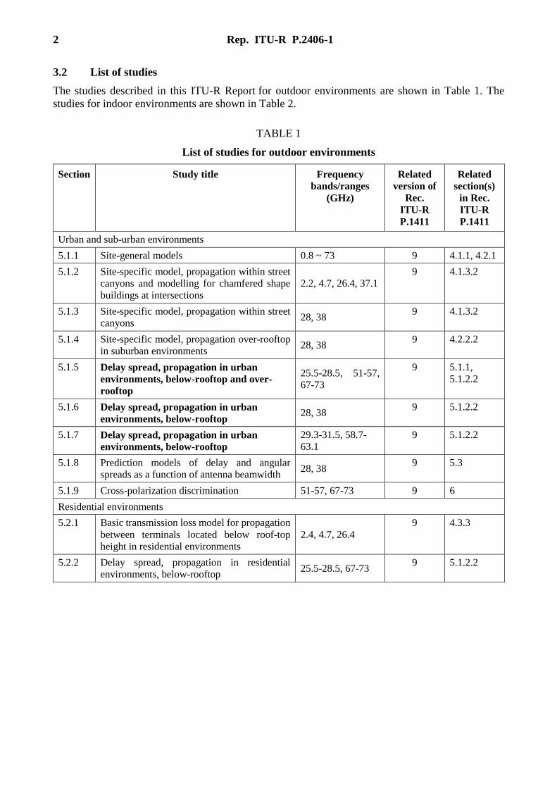
3.2 List of studies
The studies described in this ITU-R Report for outdoor environments are shown in Table 1. The
studies for indoor environments are shown in Table 2.
TABLE 1
List of studies for outdoor environments
Section Study title Frequency
bands/ranges
(GHz)
Related
version of
Rec.
ITU-R
P.1411
Related
section(s)
in Rec.
ITU-R
P.1411
Urban and sub-urban environments
5.1.1 Site-general models 0.8 ~ 73 9 4.1.1, 4.2.1
5.1.2 Site-specific model, propagation within street
canyons and modelling for chamfered shape
buildings at intersections
2.2, 4.7, 26.4, 37.1
9 4.1.3.2
5.1.3 Site-specific model, propagation within street
canyons 28, 38
9 4.1.3.2
5.1.4 Site-specific model, propagation over-rooftop
in suburban environments 28, 38
9 4.2.2.2
5.1.5 Delay spread, propagation in urban
environments, below-rooftop and over-
rooftop
25.5-28.5, 51-57,
67-73
9 5.1.1,
5.1.2.2
5.1.6 Delay spread, propagation in urban
environments, below-rooftop 28, 38
9 5.1.2.2
5.1.7 Delay spread, propagation in urban
environments, below-rooftop
29.3-31.5, 58.7-
63.1
9 5.1.2.2
5.1.8 Prediction models of delay and angular
spreads as a function of antenna beamwidth 28, 38
9 5.3
5.1.9 Cross-polarization discrimination 51-57, 67-73 9 6
Residential environments
5.2.1 Basic transmission loss model for propagation
between terminals located below roof-top
height in residential environments
2.4, 4.7, 26.4
9 4.3.3
5.2.2 Delay spread, propagation in residential
environments, below-rooftop 25.5-28.5, 67-73
9 5.1.2.2
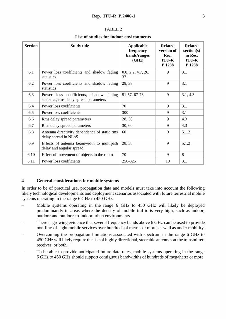
Rep. ITU-R P.2406-1 3
TABLE 2
List of studies for indoor environments
Section Study title Applicable
frequency
bands/ranges
(GHz)
Related
version of
Rec.
ITU-R
P.1238
Related
section(s)
in Rec.
ITU-R
P.1238
6.1 Power loss coefficients and shadow fading
statistics
0.8, 2.2, 4.7, 26,
37
9 3.1
6.2 Power loss coefficients and shadow fading
statistics
28, 38 9 3.1
6.3 Power loss coefficients, shadow fading
statistics, rms delay spread parameters
51-57, 67-73 9 3.1, 4.3
6.4 Power loss coefficients 70 9 3.1
6.5 Power loss coefficients 300 9 3.1
6.6 Rms delay spread parameters 28, 38 9 4.3
6.7 Rms delay spread parameters 30, 60 9 4.3
6.8 Antenna directivity dependence of static rms
delay spread in NLoS 60 9 5.1.2
6.9 Effects of antenna beamwidth to multipath
delay and angular spread
28, 38 9 5.1.2
6.10 Effect of movement of objects in the room 70 9 8
6.11 Power loss coefficients 250-325 10 3.1
4 General considerations for mobile systems
In order to be of practical use, propagation data and models must take into account the following
likely technological developments and deployment scenarios associated with future terrestrial mobile
systems operating in the range 6 GHz to 450 GHz:
– Mobile systems operating in the range 6 GHz to 450 GHz will likely be deployed
predominantly in areas where the density of mobile traffic is very high, such as indoor,
outdoor and outdoor-to-indoor urban environments.
– There is growing evidence that several frequency bands above 6 GHz can be used to provide
non-line-of-sight mobile services over hundreds of metres or more, as well as under mobility.
– Overcoming the propagation limitations associated with spectrum in the range 6 GHz to
450 GHz will likely require the use of highly directional, steerable antennas at the transmitter,
receiver, or both.
– To be able to provide anticipated future data rates, mobile systems operating in the range
6 GHz to 450 GHz should support contiguous bandwidths of hundreds of megahertz or more.
4 Rep. ITU-R P.2406-1
5 Studies for outdoor environments
5.1 Urban and suburban environments
5.1.1 Study 1: Site-general models (Frequency range: variable in 0.8 ~ 73 GHz)
5.1.1.1 Executive summary
This section provides additional information related to the development of site-general models for
urban and suburban environments included in Recommendation ITU-R P.1411.
5.1.1.2 Background and proposal
The site-general model is provided by the following equation:
𝑃𝐿(𝑑, 𝑓) = 10α log10(𝑑) + β + 10γ log10(𝑓) + 𝑁(0,σ) (dB) (1)
where:
𝑑: 3D direct distance between the transmitting and receiving stations (m)
𝑓: operating frequency (GHz)
α: coefficient associated with the increase of the basic transmission loss with
distance
β: coefficient associated with the offset value of the basic transmission loss
γ: coefficient associated with the increase of the basic transmission loss with
frequency
𝑁(0,σ): Gaussian distribution with standard deviation σ.
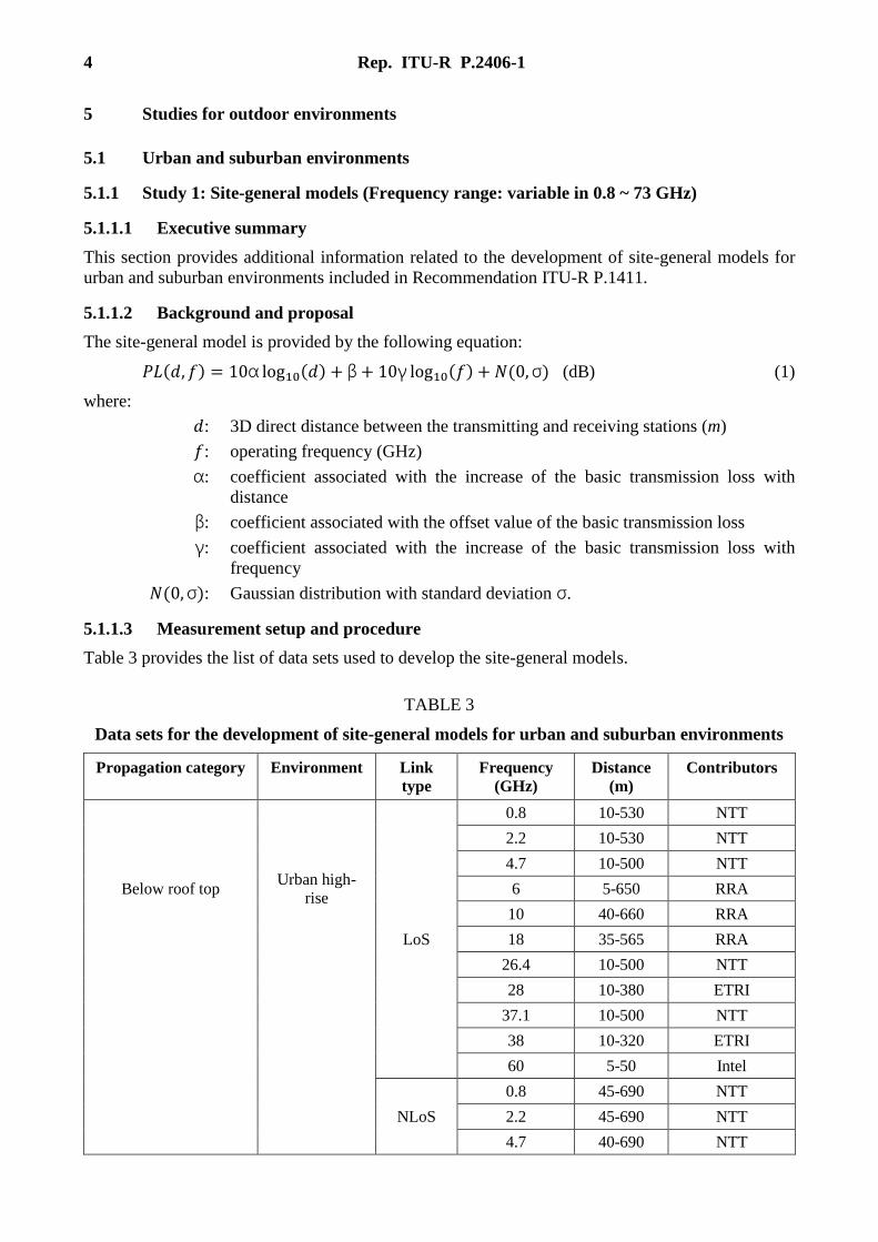
5.1.1.3 Measurement setup and procedure
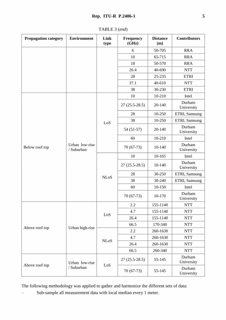
Table 3 provides the list of data sets used to develop the site-general models.
TABLE 3
Data sets for the development of site-general models for urban and suburban environments
Propagation category Environment Link
type
Frequency
(GHz)
Distance
(m)
Contributors
Below roof top Urban high-
rise
LoS
0.8 10-530 NTT
2.2 10-530 NTT
4.7 10-500 NTT
6 5-650 RRA
10 40-660 RRA
18 35-565 RRA
26.4 10-500 NTT
28 10-380 ETRI
37.1 10-500 NTT
38 10-320 ETRI
60 5-50 Intel
NLoS
0.8 45-690 NTT
2.2 45-690 NTT
4.7 40-690 NTT
Rep. ITU-R P.2406-1 5
TABLE 3 (end)
Propagation category Environment Link
type
Frequency
(GHz)
Distance
(m)
Contributors
6 50-705 RRA
10 65-715 RRA
18 50-570 RRA
26.4 40-690 NTT
28 25-235 ETRI
37.1 40-610 NTT
38 30-230 ETRI
Below roof top Urban low-rise
/ Suburban
LoS
10 10-210 Intel
27 (25.5-28.5) 20-140 Durham
University
28 10-250 ETRI, Samsung
38 10-250 ETRI, Samsung
54 (51-57) 20-140 Durham
University
60 10-210 Intel
70 (67-73) 10-140 Durham
University
NLoS
10 10-165 Intel
27 (25.5-28.5) 10-140 Durham
University
28 30-250 ETRI, Samsung
38 30-240 ETRI, Samsung
60 10-150 Intel
70 (67-73) 10-170 Durham
University
Above roof top Urban high-rise
LoS
2.2 155-1140 NTT
4.7 155-1140 NTT
26.4 155-1140 NTT
66.5 170-340 NTT
NLoS
2.2 260-1630 NTT
4.7 260-1630 NTT
26.4 260-1630 NTT
66.5 260-340 NTT
Above roof top Urban low-rise
/ Suburban LoS
27 (25.5-28.5) 55-145 Durham
University
70 (67-73) 55-145 Durham
University
The following methodology was applied to gather and harmonize the different sets of data:
– Sub-sample all measurement data with local median every 1 meter.

6 Rep. ITU-R P.2406-1
– Develop a single propagation model encompassing all available frequencies per environment
(urban high-rise, urban low-rise/suburban) and condition (below-rooftop, above-rooftop).
– For each environment and condition, use a common distance range available across all
available data sets and frequencies for basic transmission loss fitting. However the minimum
and maximum distance range was used for distance range applicability of the models (e.g.
the min-max ranges for urban high-rise NLoS below-rooftop were 30-715 m, while the
common distance range based on which basic transmission loss fitting was performed, was
65-230 m).
– A 10 dB minimum SNR level above noise-floor was applied on every data set.
– All basic transmission loss measurements were given with respect to the 3D direct distance
between the Tx and Rx antennas.
5.1.1.4 Validation results
Basic transmission loss obtained for different environments and situations, based on all data sets and
the methodology above, are depicted in the following Figures:
– Figure 1: LoS situations in below-rooftop urban and suburban environments.
– Figure 2: NLoS situations in below-rooftop urban environments.
– Figure 3: NLoS situations in below-rooftop suburban environments.
– Figure 4: LoS situations in over-rooftop urban and suburban environments.
– Figure 5: NLoS situations in over-rooftop urban environments.
FIGURE 1
Basic transmission loss for LoS in below-rooftop urban and suburban environments

Rep. ITU-R P.2406-1 7
FIGURE 2
Basic transmission loss for NLoS in below-rooftop urban environments
FIGURE 3
Basic transmission loss for NLoS in below-rooftop suburban environments

8 Rep. ITU-R P.2406-1
FIGURE 4
Basic transmission loss for LoS in above-rooftop urban and suburban environments
FIGURE 5
Basic transmission loss for NLoS in above-rooftop urban environments
5.1.1.5 Summary of the results
The results from the different data sets showed consistent behaviour across all frequency ranges for
both LoS and NLoS situations in the different environments studied. The resulting coefficients (α, β,
γ, σ) associated with the model have been included in Recommendation ITU-R P.1411.

Rep. ITU-R P.2406-1 9
5.1.2 Study 2: Site-specific model, propagation within street canyons and modelling for
chamfered shape buildings at intersections (Frequency bands: 2.2, 4.7, 26.4, 37.1 GHz)
5.1.2.1 Executive summary
This section provides additional information on the site-specific model for propagation within street
canyons, included in Recommendation ITU-R P.1411. This study focuses on the extension of the
upper frequency limit of the model to 37.1 GHz and modelling for chamfered shape buildings at
intersections.
5.1.2.2 Background and proposal
5.1.2.2.1 Site-specific model for propagation below-rooftop within street canyons
The site-specific model is provided by the following expression:
(2)
(3)
(4)
where:
𝐿𝑁𝐿𝑜𝑆2: total basic transmission loss (dB)
𝐿𝐿𝑜𝑆: basic transmission loss before the corner region (dB)
𝐿𝑐: basic transmission loss expression at the corner region (dB)
𝐿𝑎𝑡𝑡: basic transmission loss expression after the corner region (dB)
𝑑𝑐𝑜𝑟𝑛𝑒𝑟: distance of the corner region (m)
𝐿𝑐𝑜𝑟𝑛𝑒𝑟: basic transmission loss at the corner region (dB)
𝑤1: street width at the position of the Station 1 (m)
𝑤2: street width at the position of the Station 2 (m)
𝑥1: distance from Station 1 to the corner region (m)
𝑥2: distance from the corner region to Station 2 (m).
LLoS is the basic transmission loss in the LoS street for x1 (> 20 m). In equation (3), Lcorner is given as
20 dB in an urban environment and 30 dB in a residential environment. And dcorner is 30 m in both
environments.
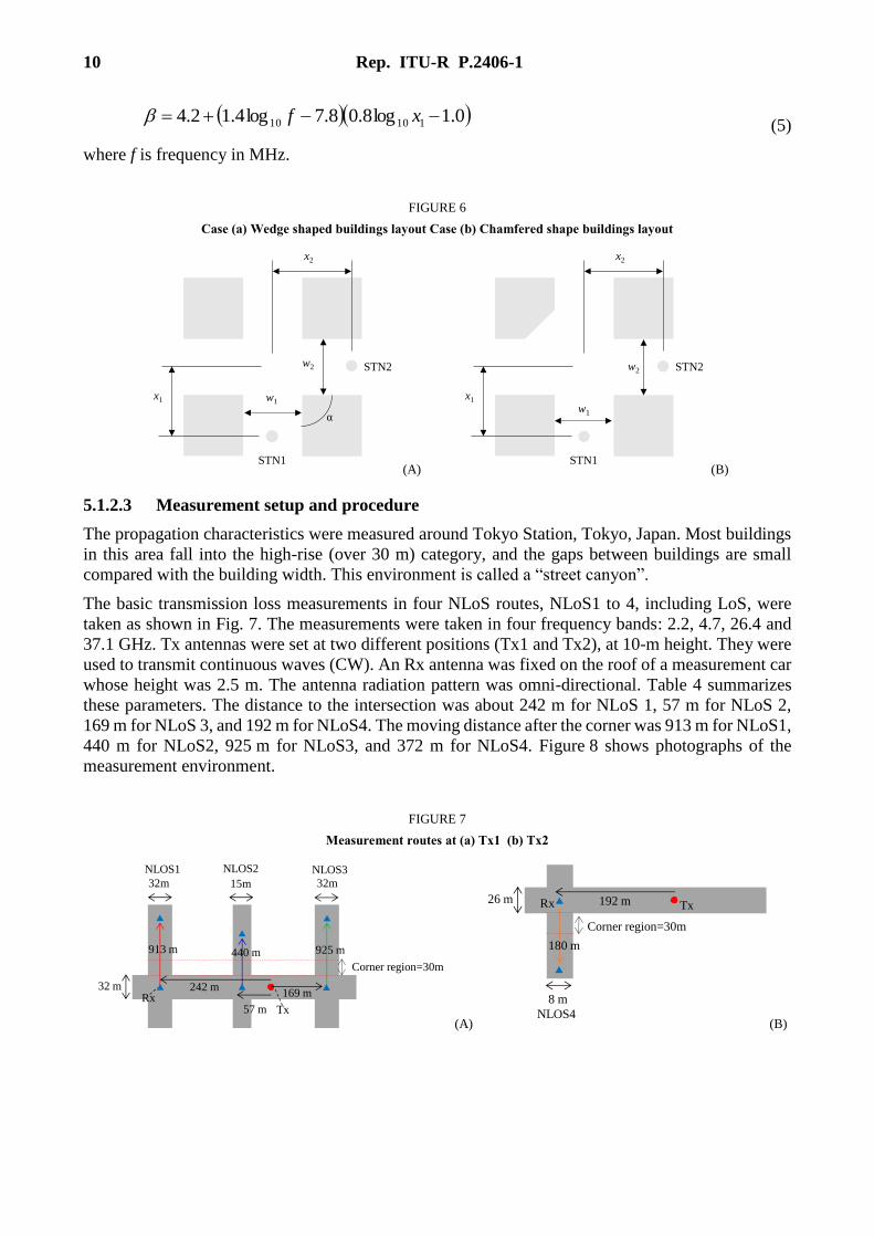
5.1.2.2.2 Basic transmission loss model for chamfered shape building at intersection
In equation (4), β = 6 in urban and residential environments for wedge-shaped buildings at four
corners of the intersection as illustrated in case (a) of Fig. 6. If a particular building is chamfered at
the intersection in urban environments as illustrated in case (b) of Fig. 6, β is calculated by equation
(5). Because the specular reflection paths from chamfered-shape buildings significantly affect basic
transmission loss in NLoS region, the basic transmission loss for case (b) is different from that for
case (a).
attcLoSNLoS LLLL 2
cornercorner
cornercorner
corner
c
dwxL
dwxwwxd
L
L
12
12122log1log
12
121121010
corner
cornercorneratt
dwx
dwxdwx
xx
L
12/0
12/2/
log10
12
1211
2110
10 Rep. ITU-R P.2406-1
(5)
where f is frequency in MHz.
FIGURE 6
Case (a) Wedge shaped buildings layout Case (b) Chamfered shape buildings layout
(A) (B)
5.1.2.3 Measurement setup and procedure
The propagation characteristics were measured around Tokyo Station, Tokyo, Japan. Most buildings
in this area fall into the high-rise (over 30 m) category, and the gaps between buildings are small
compared with the building width. This environment is called a “street canyon”.
The basic transmission loss measurements in four NLoS routes, NLoS1 to 4, including LoS, were
taken as shown in Fig. 7. The measurements were taken in four frequency bands: 2.2, 4.7, 26.4 and
37.1 GHz. Tx antennas were set at two different positions (Tx1 and Tx2), at 10-m height. They were
used to transmit continuous waves (CW). An Rx antenna was fixed on the roof of a measurement car
whose height was 2.5 m. The antenna radiation pattern was omni-directional. Table 4 summarizes
these parameters. The distance to the intersection was about 242 m for NLoS 1, 57 m for NLoS 2,
169 m for NLoS 3, and 192 m for NLoS4. The moving distance after the corner was 913 m for NLoS1,
440 m for NLoS2, 925 m for NLoS3, and 372 m for NLoS4. Figure 8 shows photographs of the
measurement environment.
FIGURE 7
Measurement routes at (a) Tx1 (b) Tx2
(A) (B)
0.1log8.08.7log4.12.4 11010 xf
STN1
α
STN2
x1
x2
w1
w2
STN1
STN2
x1
x2
w1
w2
Corner region=30m
32m 15m 32m
242 m
57 m
169 mRx32 m
913 m 440 m 925 m
Tx
NLOS1 NLOS2 NLOS3
8 m
192 m26 m
Corner region=30m
180 m
NLOS4
TxRx

Rep. ITU-R P.2406-1 11
TABLE 4
Measurement Parameters
Measured frequency (GHz) 2.2, 4.7, 26.4 and 37.1 (CW)
Antenna radiation pattern Omni-directional in horizontal plane for both Tx and Rx
Antenna gain Around 2 dBi for each antenna
Tx antenna height 10 m from the ground
Rx antenna height 2.5 m from the ground
FIGURE 8
View from (a) Tx1 (b) Tx2
(A) (B)
In a second measurement campaign, the basic transmission loss measurements were taken as shown
in Fig. 9. The measurements were taken in four frequency bands: 2.2, 4.7, 26.4 and 37.1 GHz. Tx
antennas were set at 10 m height. They were used to transmit continuous waves (CW). An Rx antenna
was fixed on the roof of a measurement car whose height was 2.5 m. The antenna radiation pattern
was omni-directional. Table 5 summarizes these parameters. The distance to the intersection was
about 169 m. The moving distance after the corner was 431 m.
FIGURE 9
Measurement route
w1=
32 m
Corner region
dcorner=30m
w2=32m
Tx
Rx
x1=169m
x2=
431m
NLOS
region
12 Rep. ITU-R P.2406-1
TABLE 5
Measurement parameters
Measured frequency (GHz) 2.2, 4.7, 26.4 and 37.1 (CW)
Antenna radiation pattern Omni-directional in horizontal plane for both Tx and Rx
Tx antenna height 10 m from the ground
Rx antenna height 2.5 m from the ground
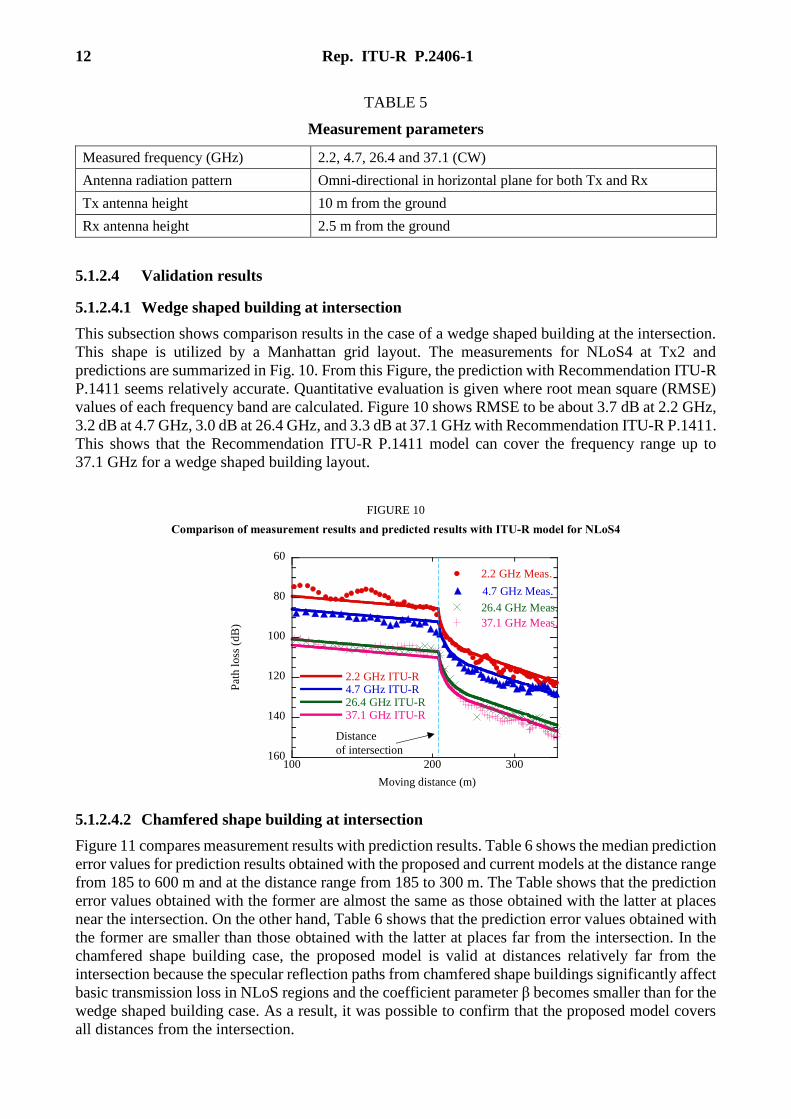
5.1.2.4 Validation results
5.1.2.4.1 Wedge shaped building at intersection
This subsection shows comparison results in the case of a wedge shaped building at the intersection.
This shape is utilized by a Manhattan grid layout. The measurements for NLoS4 at Tx2 and
predictions are summarized in Fig. 10. From this Figure, the prediction with Recommendation ITU-R
P.1411 seems relatively accurate. Quantitative evaluation is given where root mean square (RMSE)
values of each frequency band are calculated. Figure 10 shows RMSE to be about 3.7 dB at 2.2 GHz,
3.2 dB at 4.7 GHz, 3.0 dB at 26.4 GHz, and 3.3 dB at 37.1 GHz with Recommendation ITU-R P.1411.
This shows that the Recommendation ITU-R P.1411 model can cover the frequency range up to
37.1 GHz for a wedge shaped building layout.
FIGURE 10
Comparison of measurement results and predicted results with ITU-R model for NLoS4
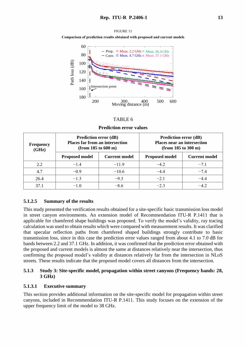
5.1.2.4.2 Chamfered shape building at intersection
Figure 11 compares measurement results with prediction results. Table 6 shows the median prediction
error values for prediction results obtained with the proposed and current models at the distance range
from 185 to 600 m and at the distance range from 185 to 300 m. The Table shows that the prediction
error values obtained with the former are almost the same as those obtained with the latter at places
near the intersection. On the other hand, Table 6 shows that the prediction error values obtained with
the former are smaller than those obtained with the latter at places far from the intersection. In the
chamfered shape building case, the proposed model is valid at distances relatively far from the
intersection because the specular reflection paths from chamfered shape buildings significantly affect
basic transmission loss in NLoS regions and the coefficient parameter β becomes smaller than for the
wedge shaped building case. As a result, it was possible to confirm that the proposed model covers
all distances from the intersection.
60
80
100
120
140
160100 200 300
2.2 GHz Meas.
2.2 GHz ITU-R
4.7 GHz Meas.
26.4 GHz Meas.
37.1 GHz Meas.
4.7 GHz ITU-R26.4 GHz ITU-R 37.1 GHz ITU-R
Path
lo
ss (
dB
)
Moving distance (m)
Distance
of intersection
Rep. ITU-R P.2406-1 13
FIGURE 11
Comparison of prediction results obtained with proposed and current models
TABLE 6
Prediction error values
Frequency
(GHz)
Prediction error (dB)
Places far from an intersection
(from 185 to 600 m)
Prediction error (dB)
Places near an intersection
(from 185 to 300 m)
Proposed model Current model Proposed model Current model
2.2 −1.4 −11.9 −4.2 −7.1
4.7 −0.9 −10.6 −4.4 −7.4
26.4 −1.3 −9.3 −2.1 −4.4
37.1 −1.0 −8.6 −2.3 −4.2
5.1.2.5 Summary of the results
This study presented the verification results obtained for a site-specific basic transmission loss model
in street canyon environments. An extension model of Recommendation ITU-R P.1411 that is
applicable for chamfered shape buildings was proposed. To verify the model’s validity, ray tracing
calculation was used to obtain results which were compared with measurement results. It was clarified
that specular reflection paths from chamfered shaped buildings strongly contribute to basic
transmission loss, since in this case the prediction error values ranged from about 4.1 to 7.0 dB for
bands between 2.2 and 37.1 GHz. In addition, it was confirmed that the prediction error obtained with
the proposed and current models is almost the same at distances relatively near the intersection, thus
confirming the proposed model’s validity at distances relatively far from the intersection in NLoS
streets. These results indicate that the proposed model covers all distances from the intersection.
5.1.3 Study 3: Site-specific model, propagation within street canyons (Frequency bands: 28,
3 GHz)
5.1.3.1 Executive summary
This section provides additional information on the site-specific model for propagation within street
canyons, included in Recommendation ITU-R P.1411. This study focuses on the extension of the
upper frequency limit of the model to 38 GHz.
60
80
100
120
140
160
180200 300 400 500 600
Pat
h l
oss
(d
B)
Moving distance (m)
Meas. 2.2 GHz
Meas. 4.7 GHzMeas. 26.4 GHzMeas. 37.1 GHzConv.
Prop.
Intersection point

14 Rep. ITU-R P.2406-1
5.1.3.2 Background and proposal
The site-specific model is provided by the following expression:
(6)
(7)
(8)
where:
𝐿𝑁𝐿𝑜𝑆2: total basic transmission loss (dB)
𝐿𝐿𝑜𝑆 : basic transmission loss before the corner region (dB)
𝐿𝑐 : basic transmission loss expression at the corner region (dB)
𝐿𝑎𝑡𝑡 : basic transmission loss expression after the corner region (dB)
𝑑𝑐𝑜𝑟𝑛𝑒𝑟 : distance of the corner region (m)
𝐿𝑐𝑜𝑟𝑛𝑒𝑟 : basic transmission loss at the corner region (dB)
𝑤1 : street width at the position of the Station 1 (m)
𝑤2 : street width at the position of the Station 2 (m)
𝑥1 : distance from Station 1 to the corner region (m)
𝑥2 : distance from the corner region to Station 2 (m).
LLoS is the basic transmission loss in the LoS street for x1 (> 20 m). In equation (7), Lcorner is given as
20 dB in an urban environment and 30 dB in a residential environment. And dcorner is 30 m in both
environments.
Note that the applicable frequency range was from 2 to 16 GHz in Recommendation ITU-R P.1411-8
and the range was extended up to 38 GHz in Recommendation ITU-R P.1411-9 based on the study
described here.
5.1.3.3 Measurement setup and procedure
Figure 12 shows the 28/38 GHz channel sounder, where detailed specification relevant to basic
transmission loss measurements is listed in Table 7.
attcLoSNLoS LLLL 2
cornercorner
cornercorner
corner
c
dwxL
dwxwwxd
L
L
12
12122log1log
12
121121010
corner
cornercorneratt
dwx
dwxdwx
xx
L
12/0
12/2/
log10
12
1211
2110

Rep. ITU-R P.2406-1 15
FIGURE 12
Measurement equipment
TABLE 7
Measurement equipment specification
System parameters Specifications
Centre frequency 28 and 38 GHz
Maximum TX RF power
(w/o antenna gain)
29 dBm (28 GHz)
21 dBm (38 GHz)
AGC range 60 dB
Measureable basic transmission loss range 170 dB
Measurement campaigns were conducted in urban street environments with the following
configurations:
– 4 m TX height and 1.5 m RX height;
– 30-50 m building height and 30 m street width;
– Two different TX locations.
Figure 13(a) shows the measurement environment, which can be considered as a street canyon
environment. This street is in a downtown metro station in Daejeon near the City Hall. The average
street width is 30 m and the building height is between 30 m and 50 m.
Figure 13(b) shows the measurement layout on which the location of TX and the measurement route
of RX are marked. During the measurements, TX was held stationary and RX was moved along the
designated measurement route. As can be seen, the RX measurement route is perpendicular to the TX
street, the corner is the NLoS obstruction source. To see the effect of the distance between the corner
and TX, measurements were conducted in two different TX locations: 65 m (denoted by TX1) and
105 m (denoted by TX2). Considering two frequencies (28 and 38 GHz) and two TX locations, four
sets of measurements were collected.

16 Rep. ITU-R P.2406-1
FIGURE 13
(a) Measurement street environment (b) Measurement layout
(A) (B)
5.1.3.4 Validation results
This section retraces the archived documents relevant to the Recommendation ITU-R P.1411 NLoS
basic transmission loss model. The first proposal was made in 2001, in which a then-new propagation
model for the SHF band was proposed based on 3.35, 8.45 and 15.75 GHz measurements. By
comparing these frequency band measurements to the then-existing UHF propagation model, it
claimed that the propagation behaviour in the SHF band is different, and proposed an initial model.
With continuing discussions in the Working Party 3K meetings, the current form of the model was
adopted in 2007.
If measurement conditions of previous measurements and results are briefly reviewed, their 𝑥1
distance (distance between TX and the corner) is 65 and 430 m (ours is 65 and 105 m). With their 𝑥1
distance setting, they obtained 𝐿𝑐𝑜𝑟𝑛𝑒𝑟 and β, as listed in Table 8. Note that since they have only two
TX-location measurements, the “ranges” in Table 8 were derived from only these two measurements.
TABLE 8
Rec. ITU-R P.1411 NLoS basic transmission loss model parameters for
urban environments obtained from previous measurements
Frequency (GHz) 𝑳𝒄𝒐𝒓𝒏𝒆𝒓 (dB) 𝛃
3.35 16-17 4.7-12
8.45 22-28 5.2
15.75 22-23 4.2-12
Rec. ITU-R P.1411 nominal (typical) value 20 6
Although the literature and archived documents were searched, it was not possible to find a nominal
(typical) value determination process, which was set to 𝐿𝑐𝑜𝑟𝑛𝑒𝑟 = 20 dB and β = 6 for urban
environments. According to a previous contribution in 2005, the “typical value” of β was chosen as
8, since the range of β was from 4.7 to 12. In another contribution (2006), the typical value of β was
changed to 6 since the range was adjusted from 4.2 to 12. A similar argument is applied to 𝐿𝑐𝑜𝑟𝑛𝑒𝑟.
According to the two contributions mentioned above, the typical value of 𝐿𝑐𝑜𝑟𝑛𝑒𝑟 was chosen as
20 dB in urban environments, considering that measurements were given by 16-28 dB. The reason
for this choice was drawn from arguments regarding the importance of cell-edge interference in
practical cellular network designs, which emphasized the importance of the lower bound. It can be
observed that the parameter range from the measurements as listed in Table 9 are also in, or close to,
Rep. ITU-R P.2406-1 17
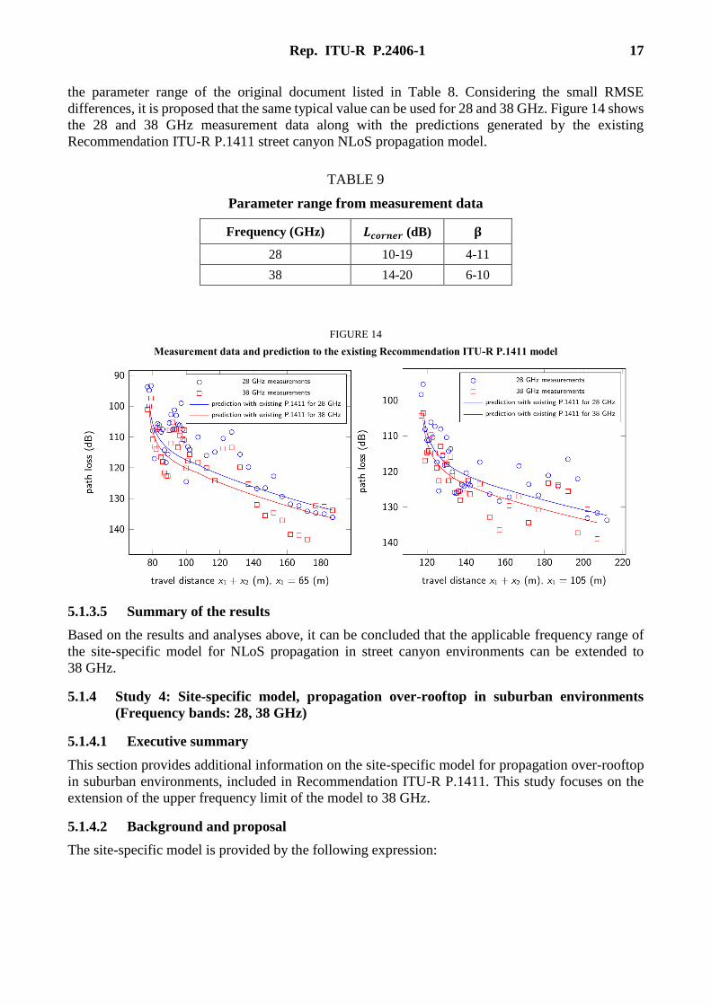
the parameter range of the original document listed in Table 8. Considering the small RMSE
differences, it is proposed that the same typical value can be used for 28 and 38 GHz. Figure 14 shows
the 28 and 38 GHz measurement data along with the predictions generated by the existing
Recommendation ITU-R P.1411 street canyon NLoS propagation model.
TABLE 9
Parameter range from measurement data
Frequency (GHz) 𝑳𝒄𝒐𝒓𝒏𝒆𝒓 (dB) 𝛃
28 10-19 4-11
38 14-20 6-10
FIGURE 14
Measurement data and prediction to the existing Recommendation ITU-R P.1411 model
5.1.3.5 Summary of the results
Based on the results and analyses above, it can be concluded that the applicable frequency range of
the site-specific model for NLoS propagation in street canyon environments can be extended to
38 GHz.
5.1.4 Study 4: Site-specific model, propagation over-rooftop in suburban environments
(Frequency bands: 28, 38 GHz)
5.1.4.1 Executive summary
This section provides additional information on the site-specific model for propagation over-rooftop
in suburban environments, included in Recommendation ITU-R P.1411. This study focuses on the
extension of the upper frequency limit of the model to 38 GHz.
5.1.4.2 Background and proposal
The site-specific model is provided by the following expression:

18 Rep. ITU-R P.2406-1
(9)
where:
𝑑: 3D direct distance between the transmitting and receiving stations (m)
λ: wavelength (m)
𝑑0 : distance separating the direct and reflected wave dominant regions (m)
𝐿0𝑛: basic transmission loss expression for the reflected wave dominant region (dB)
𝑑𝑅𝐷: distance separating the reflected and diffracted wave dominant regions (m)
𝐿𝑑𝑅𝐷: basic transmission loss expression for the diffracted wave dominant region (dB).
Equations that further detail this model can be found in Recommendation ITU-R P.1411.
5.1.4.3 Measurement setup and procedure
The measurement campaign was conducted in Gwanpyeong, Daejeon, Republic of Korea.
Transmitter (Tx) was installed on the top of a 30 m high building. The average height of buildings
surrounding Tx was 11 m and the average width of the streets was 10 m. Receiver (Rx) was set on
the streets and its height was 1.7 m. The beam width of Tx was 30 degrees and an omni-directional
receive antenna was used. In Fig. 15(a), Tx and Rx which were used in the measurement campaign
are shown. To obtain various transmission losses with respect to distance, Rx was consistently moved
in small increments. Thus, Rx routes were made. The location of Tx and Rx routes are provided in
Fig. 15(b). The frequency band of 28 GHz and 38 GHz were measured at the same streets, thus the
number of Rx routes for 28 GHz and 38 GHz are the same. However, the number of total transmission
loss samples are different (28 GHz: 810, 38 GHz, 666). It is assumed that a limitation of measurement
performance makes the difference.
FIGURE 15
(a) View from Tx and Rx (b) Locations of Tx and Rx
(A) (B)
5.1.4.4 Validation results
In Fig. 16, a comparison of the measurements and Recommendation ITU-R P.1411 over rooftops
basic transmission loss model are provided. The parameters of Recommendation ITU-R P.1411 over
rooftops basic transmission loss model are shown in Table 10. As a matter of fact, every angle of
street orientation (φ) of the samples is different. However, to compare the measurements and the
basic transmission loss model, 45 degree is chosen to represent the rest of φ. The boundary between
region)dominant waved(Diffracteforlog1.32
region)dominant wave(Reflectedfor
region)dominant ve(Direct wa for4
log20
10
00
010
1
RDdRD
RDnNLoS
ddLd
d
dddL
ddd
L
RD
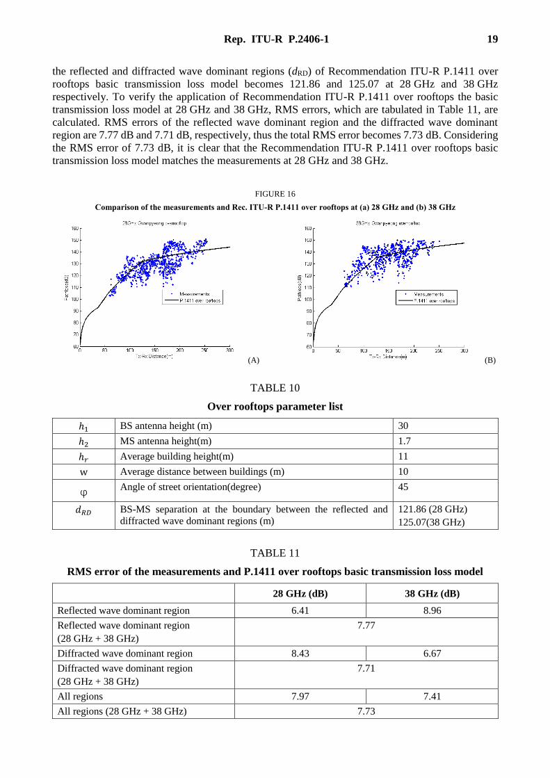
Rep. ITU-R P.2406-1 19
the reflected and diffracted wave dominant regions (dRD) of Recommendation ITU-R P.1411 over
rooftops basic transmission loss model becomes 121.86 and 125.07 at 28 GHz and 38 GHz
respectively. To verify the application of Recommendation ITU-R P.1411 over rooftops the basic
transmission loss model at 28 GHz and 38 GHz, RMS errors, which are tabulated in Table 11, are
calculated. RMS errors of the reflected wave dominant region and the diffracted wave dominant
region are 7.77 dB and 7.71 dB, respectively, thus the total RMS error becomes 7.73 dB. Considering
the RMS error of 7.73 dB, it is clear that the Recommendation ITU-R P.1411 over rooftops basic
transmission loss model matches the measurements at 28 GHz and 38 GHz.
FIGURE 16
Comparison of the measurements and Rec. ITU-R P.1411 over rooftops at (a) 28 GHz and (b) 38 GHz
(A) (B)
TABLE 10
Over rooftops parameter list
ℎ1 BS antenna height (m) 30
ℎ2 MS antenna height(m) 1.7
ℎ𝑟 Average building height(m) 11
w Average distance between buildings (m) 10
φ Angle of street orientation(degree) 45
𝑑𝑅𝐷 BS-MS separation at the boundary between the reflected and
diffracted wave dominant regions (m)
121.86 (28 GHz)
125.07(38 GHz)
TABLE 11
RMS error of the measurements and P.1411 over rooftops basic transmission loss model
28 GHz (dB) 38 GHz (dB)
Reflected wave dominant region 6.41 8.96
Reflected wave dominant region
(28 GHz + 38 GHz)
7.77
Diffracted wave dominant region 8.43 6.67
Diffracted wave dominant region
(28 GHz + 38 GHz)
7.71
All regions 7.97 7.41
All regions (28 GHz + 38 GHz) 7.73
20 Rep. ITU-R P.2406-1
5.1.4.5 Summary of the results
The results show that the reflected wave dominant region and diffracted wave dominant region are
well matched with the measurements. In addition, a total RMS error of 7.73 dB is small enough that
a higher frequency, up to 38 GHz, is applicable. As a result, it can be concluded that the
Recommendation ITU-R P.1411 over rooftops basic transmission loss model can be applied up to
38 GHz.
5.1.5 Study 5: Delay spread, propagation in urban environments, below-rooftop and over-
rooftop (Frequency bands: 25.5-28.5 GHz, 51-57 GHz, 67-73 GHz)
5.1.5.1 Executive summary
This section provides additional information for the rms delay spread values included in
Recommendation ITU-R P.1411. This study focuses on the frequency ranges 25.5-28.5 GHz,
51-57 GHz and 67-73 GHz based on measurements made in urban high-rise and low-rise
environments.
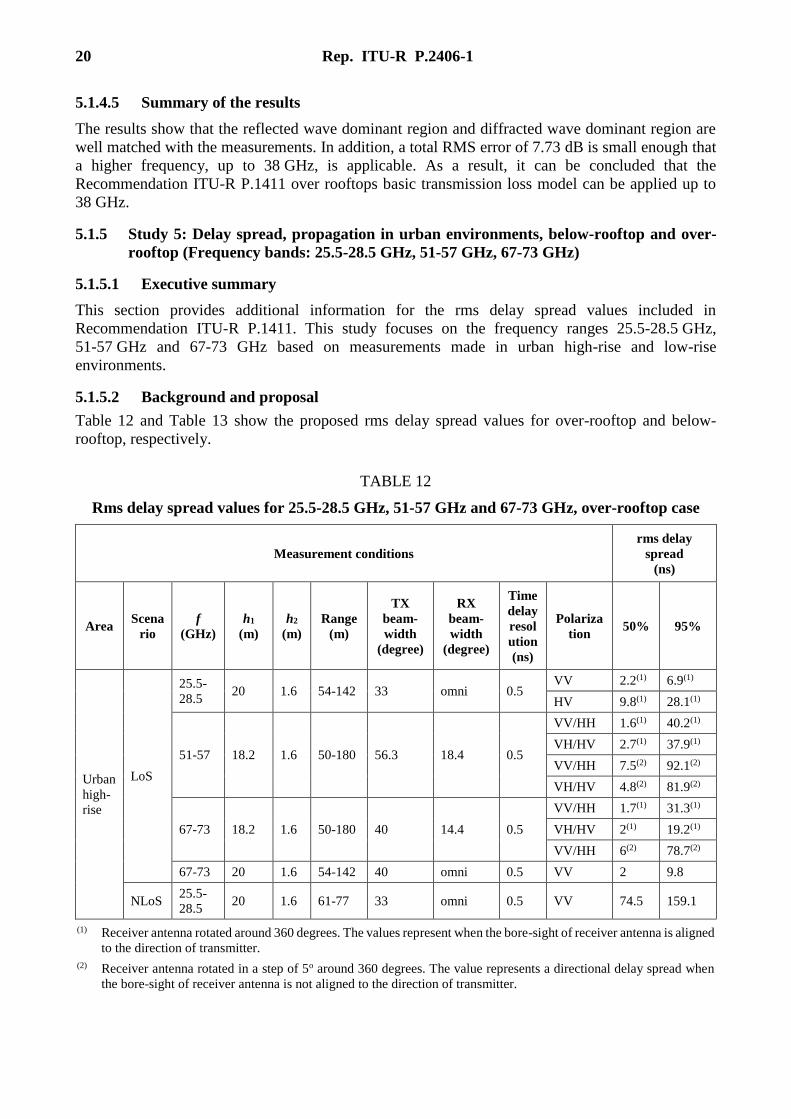
5.1.5.2 Background and proposal
Table 12 and Table 13 show the proposed rms delay spread values for over-rooftop and below-
rooftop, respectively.
TABLE 12
Rms delay spread values for 25.5-28.5 GHz, 51-57 GHz and 67-73 GHz, over-rooftop case
Measurement conditions
rms delay
spread
(ns)
Area Scena
rio
f
(GHz)
h1
(m)
h2
(m)
Range
(m)
TX
beam-
width
(degree)
RX
beam-
width
(degree)
Time
delay
resol
ution
(ns)
Polariza
tion 50% 95%
Urban
high-
rise
LoS
25.5-
28.5 20 1.6 54-142 33 omni 0.5
VV 2.2(1) 6.9(1)
HV 9.8(1) 28.1(1)
51-57 18.2 1.6 50-180 56.3 18.4 0.5
VV/HH 1.6(1) 40.2(1)
VH/HV 2.7(1) 37.9(1)
VV/HH 7.5(2) 92.1(2)
VH/HV 4.8(2) 81.9(2)
67-73 18.2 1.6 50-180 40 14.4 0.5
VV/HH 1.7(1) 31.3(1)
VH/HV 2(1) 19.2(1)
VV/HH 6(2) 78.7(2)
67-73 20 1.6 54-142 40 omni 0.5 VV 2 9.8
NLoS 25.5-
28.5 20 1.6 61-77 33 omni 0.5 VV 74.5 159.1
(1) Receiver antenna rotated around 360 degrees. The values represent when the bore-sight of receiver antenna is aligned
to the direction of transmitter.
(2) Receiver antenna rotated in a step of 5o around 360 degrees. The value represents a directional delay spread when
the bore-sight of receiver antenna is not aligned to the direction of transmitter.

Rep. ITU-R P.2406-1 21
TABLE 13
Rms delay spread values for 25.5-28.5 GHz, 51-57 GHz and 67-73 GHz, below-rooftop case
Measurement conditions rms delay spread
(ns)
Area Scena
rio
f
(GHz)
h1
(m)
h2
(m)
Range
(m)
TX
beam-
width
(degree)
RX
beam-
width
(degree)
Time
delay
resoluti
on (ns)
Polari
zation 50% 95%
Urban
low-
rise
LoS
25.5-
28.5 3 1.6 18-140 33 Omni 0.5
VV 3.5 43.6
HV 8.7 57
51-57 3 1.6 11-180 56.3 18.4 0.5
VV/H
H
0.74(1) 3(1)
VH/H
V
1.7(1) 7.5(1)
VV/H
H
11.2(2) 72.9(2)
VH/H
V
8.5(2) 40.9(2)
67-73 3 1.6 11-180 40 14.4 0.5
VV/H
H
0.6(1) 3.5(1)
VH/H
V
1.6(1) 5.9(1)
VV/H
H
8.9(2) 80(2)
VH/H
V
5(2) 39.8(2)
3 1.6 18-140 40 Omni 0.5 VV 2.6 36
NLoS
25.5-
28.5 3 1.6 40-84 33 Omni 0.5 VV
13.4 30.3
67-73 3 1.6 40-84 40 Omni 0.5 VV 10 23.7
(1) Receiver antenna was rotated around 360 degrees in measurements. The value represents a directional delay spread
when the bore-sight of receiver antenna is aligned to the direction of transmitter.
(2) Receiver antenna was rotated in a step of 5o around 360 degrees in measurements. The value represents a directional
delay spread when the bore-sight of receiver antenna is not aligned to the direction of transmitter.
5.1.5.3 Measurement setup and procedure
To study the radio channel in these wave bands, a custom designed radio channel sounder capable of
measuring with two transmit and two receive antennas has been designed [1] and used for
measurements in an outdoor environment with a transmit antenna height at ~3 m for below roof top
measurements and 18.2 m for above roof top measurements. The receiver antenna height was set at
1.6 m for all the measurements.
In a first set of measurements, horn antennas were used at the receiver with a beam width (18.4º in
the E plane and 19.7º in the H plane at 50 GHz and 14.4º in the E plane and 15.4º in the H plane at
67.5 GHz). At the transmitter two horn antennas with beam widths (56.3º in the E plane and 51.4º in
the H plane at 50 GHz and 40º in the E plane and 38º in the H plane at 67.5 GHz). To perform dual
polarisation measurements, a twist was used at one of the transmit channels and another at one of the
receive channels. To enable LoS measurements (including both cases where the bore-sight of the
receive antenna is aligned and not aligned to the direction of the transmitter) the receiver was mounted

22 Rep. ITU-R P.2406-1
on a turntable which was rotated in 5 degree steps. The measurements were performed with a 6 GHz
bandwidth with a 305 Hz waveform repetition frequency and data were acquired over 1 second for
each angle of rotation. Measurements were performed in two frequency bands: 51-57 GHz and
67-73 GHz along a number of routes in a low rise urban environment which included street canyons,
open squares, pedestrian paths and road side scenarios. The data were analysed with a 2 GHz
bandwidth, to give a 0.5 ns time delay resolution and the power delay profiles from all angles of
rotation were used to estimate the rms delay spread in the two frequency bands for 20 dB threshold.
In a second set, measurements were performed with dual polarised antennas at the transmitter and an
omni-directional antenna at the receiver with vertical polarisation. At the transmitter two horn
antennas with beam widths (40o in the E-plane and 38o in the H-plane) were used in the 67-73 GHz
band with a twist at one of the transmit channels. In addition, a new set of dual polarised transmitters
and two receivers were designed and implemented to perform measurements in the 25.5-28.5 GHz
band. The transmit antenna has a 3 dB beam width of ~36o in the H-plane and 33o in the E-plane and
the receive antenna was omni-directional. The measured environments include above rooftop and
below roof top in both residential and low rise urban environments. The measurements were
performed in both line of sight and non-line of sight where the transmitter was placed around the
corner of a street. The data were systematically collected by moving the receiver trolley over
consecutive 1 m intervals and the power delay profiles were then obtained by dividing the 1 m data
into five sections. The data were analysed with 2 GHz bandwidth to give a 0.5 ns time delay resolution
and the power delay profiles were used to estimate the rms delay spread in the two frequency bands
for 20 dB threshold using the method defined in Recommendation ITU-R P.1407.
Figure 17 shows some of the measured environments.
FIGURE 17
View of the measured environment (a) above rooftop, (b) below rooftop
(A) (B)
5.1.5.4 Validation results
For the first set of experiments described in the previous section, Table 14 gives the parameters of
the rms delay spread for the 51-57 GHz and 67-73 GHz bands for the co-polar and cross polar
antennas for the LoS case (where the bore-sight of receiver antenna is not aligned to the direction of
transmitter) for a 20 dB threshold from the maximum of the power delay profile in the street canyon
and open square environment.

Rep. ITU-R P.2406-1 23
TABLE 14
Rms delay spread (ns) for LoS
(Tx and Rx antenna directions not aligned; street canyon and open square)
(a) 52 GHz (b) 68 GHz
(a)
CDF % VV VH HV HH
50% 6.07 9.88 16.56 3.66
95% 20.98 86.44 139.48 67.62
(b)
CDF % VV VH HV HH
50% 3.39 10.16 12.43 5.53
95% 9.13 132.96 166.87 20.18
The data from all the below the roof top measured scenarios were then combined together and the
cumulative distribution function (CDF) generated for each polarisation for the two frequency bands.
The co-polarised (VV and HH) and cross-polarised (VH and HV) data for each of the two frequency
bands were then combined as shown in Fig. 18. Similarly the combined data for the over roof top
were used to generate CDF’s for the LoS and NLoS as in Fig. 19.
FIGURE 18
CDF of rms delay spread for LoS and “NLoS” (i.e. LoS but with Tx-Rx antenna directions not aligned)
for below the roof top scenario (a) 51-57 GHz, (b) 67-73 GHz
(A) (B)
FIGURE 19
CDF of rms delay spread for LoS and “NLoS” (i.e. LoS but with Tx-Rx antenna directions not aligned)
for over the roof top scenario (a) 51-57 GHz, (b) 67-73 GHz.
(A) (B)

24 Rep. ITU-R P.2406-1
For the second set of experiments described in the previous section, Fig. 20 displays the CDF of the
rms delay spread obtained from all the measured locations below rooftop environments for the two
bands (with VV at 67-73 GHz and VV co-polarised and HV cross-polarised in the 25.5-28.5 GHz
band). Similarly, Fig. 21 displays the delay spread for the above roof top scenario for LoS and only
the VV in the 25.5-28.5 GHz for the NLoS scenario due to the limited number of data points that met
the 20 dB threshold.
FIGURE 20
Rms delay spread for 20 dB threshold in the 25.5-28.5 GHz and 67-73 GHz bands for the
(a) LoS, (b) NLoS scenarios for below roof top
(A) (B)
FIGURE 21
Rms delay spread for 20 dB threshold in the 25.5-28.5 GHz and 67-73 GHz bands for the
(a) LoS, (b) NLoS scenarios for above roof top
(A) (B)
The 50% and 95% values were estimated from the CDF’s and these are summarised in Table 13.
5.1.5.5 Summary of the results
These results and analyses were used as basis to propose the new rms delay spread values.
5.1.5.6 References
[1] Salous, Sana, Feeney, Stuart, Raimundo, Xavier & Cheema, Adnan (2016). Wideband MIMO
channel sounder for radio measurements in the 60 GHz band. IEEE Transactions on Wireless
Communications 15(4): 2825-2832.
5.1.6 Study 6: Delay spread, propagation in urban environments, below-rooftop
(Frequency bands: 28, 38 GHz)
5.1.6.1 Executive summary
This section provides additional information for the rms delay spread values included in
Recommendation ITU-R P.1411. This study focuses on the frequency bands 28 GHz and 38 GHz
based on measurements made in urban low-rise and very high-rise environments.

Rep. ITU-R P.2406-1 25
5.1.6.2 Background and proposal
Table 15 shows the proposed rms delay spread values.
TABLE 15
Rms delay spread values for 28 GHz and 38 GHz, below-rooftop case
Measurement conditions
rms delay
spread
(ns)
Area Scena
rio
f
(GHz)
h1
(m)
h2
(m)
Range
(m)
TX
beam-
width
(degree)
RX
beam-
width
(degree)
Time
delay
resoluti
on (ns)
Polariza
tion 50% 95%
Urban
low-
rise
LoS
28 4 1.5 100-
400 30 10 2 VV 1.9(1) 5.9(1)
38 4 1.5 50-400 30 10 2 VV 1.2(1) 4.8(1)
28 4 1.5 90-350 30 10 2 VV 48.5(2) 112.4(2)
38 4 1.5 90-250 30 10 2 VV 25.9(2) 75.0(2)
Urban
very
high-
rise
LoS 28 4 1.5 50-350 30 10 2 VV 1.7(1) 7.8(1)
38 4 1.5 20-350 30 10 2 VV 1.6(1) 7.4(1)
NLoS 28 4 1.5 90-350 30 10 2 VV 67.2(2) 177.9(2)
38 4 1.5 90-350 30 10 2 VV 57.9(2) 151.6(2)
(1) Receiver antenna was rotated around 360 degrees in measurements. The value represents a directional delay spread
when the bore-sight of receiver antenna is aligned to the direction of transmitter.
(2) Receiver antenna was rotated around 360 degrees in measurements. The value represents a directional delay spread
regardless of antenna alignment.
5.1.6.3 Measurement setup and procedure
The delay spread measurement campaign has been performed using the millimetre wave channel
sounder, which was developed by Electronics and Telecommunications Research Institute (ETRI),
Republic of Korea [1]. Figure 22 is a wideband channel sounder for measuring the spatial and
temporal channel characteristics of 500 MHz bandwidth in the 28/38 GHz band. The RF modules
including antenna can rotates from 0° to 360° horizontally and tilts from −90° to 90° vertically. Table
16 shows detailed specifications of the channel sounder.
FIGURE 22
28/38 GHz wideband channel sounding system

26 Rep. ITU-R P.2406-1
TABLE 16
Specifications of the channel sounder
Description Specifications
Carrier Frequency 28/38 GHz
Channel Bandwidth 500 MHz
PN Code length 4 095 chips
Sliding factor 12,500
Receiver chip rate 499.96 MHz
Maximum TX Power 29/21 dBm
Automatic Gain Control range < 60 dB
The measurement campaign was done in Seoul and Daejeon of the Republic Korea. Seoul is an urban
very high-rise environment, which has a downtown area with 50-200 m height buildings and 54 m
wide streets. Daejeon is an urban low-rise environment, which has a small town area with 3~5 story
buildings (11~14 m height) and 18 m wide streets.
Directional horn antennas were used for 28/38 GHz. They have a gain of 15.4 dBi (30° HPBW, Half
Power Beam Width) at TX and 24.4 dBi (10° HPBW) at RX for 28 GHz, and 16.4 dBi (30° HPBW)
antenna at TX and 24.6 dBi (10° HPBW) antenna at RX for 38 GHz. The azimuthal rotation step size
was 10° for 28 GHz and 9° for 38 GHz from 0° to 360°. The elevation range was –10° to 10° for both
bands. The TX antenna was installed at a height of 4 m (assumed lamp-post level) and the RX antenna
at 1.5 m for both bands
The measurements were taken at 17 positions (7 LoS/11 NLoS) at the Seoul site and 21 positions
(6 LoS/15 NLoS) at the Daejeon site for 28 GHz, and 35 positions (17 LoS/18 NLoS) at the Seoul
site and 26 (9 LoS/17 NLoS) positions at the Daejeon site for 38 GHz. In the NLoS case, each position
has 36 × 3 = 108 samples for 28 GHz and 40 × 3 = 120 samples for 38 GHz. However, in the LoS
case, it refers to the case when the antennas are aligned; each position has 3 × 3 = 9 samples for both
bands. So the positions for LoS and NLoS are different from each other at 28/38 GHz.
5.1.6.4 Validation results
Figure 23 shows CDFs of all measurement results at each site and at each band. The typical rms delay
spread values of 50% and 95% of cumulative probability are shown in Table 15. The threshold value
of 20 dB is used for the rms delay spread calculation.
FIGURE 23
Cumulative probability of RMS delay spread in urban environments: (a) CDF of LoS (b) CDF of NLoS
(A) (B)
Rep. ITU-R P.2406-1 27
5.1.6.5 Summary of the results
These results and analyses were used as a basis to propose the new rms delay spread values.
5.1.6.6 References
[1] Jong Ho Kim, Y Yoon, Y. Chong and M Kim. "28 GHz Wideband Characteristics at Urban Area."
Vehicular Technology Conference (IEEE 82nd VTC-Fall) 2015.
5.1.7 Study 7: Delay spread, propagation in urban environments, below-rooftop
(Frequency bands: 29.3-31.5 GHz, 58.7-63.1 GHz)
5.1.7.1 Executive summary
This section provides additional information for the rms delay spread values included in
Recommendation ITU-R P.1411. This study focuses on the frequency ranges 29.3-31.5 GHz and
58.7-63.1 GHz based on measurements made in urban low-rise environments.
5.1.7.2 Background and proposal
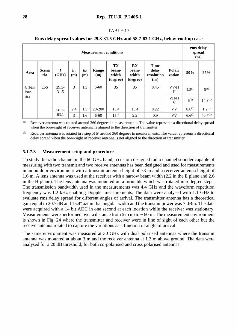
Table 17 shows the proposed rms delay spread values.
28 Rep. ITU-R P.2406-1
TABLE 17
Rms delay spread values for 29.3-31.5 GHz and 58.7-63.1 GHz, below-rooftop case
Measurement conditions
rms delay
spread
(ns)
Area Scena
rio
f
(GHz)
h1
(m)
h2
(m)
Range
(m)
TX
beam-
width
(degree)
RX
beam-
width
(degree)
Time
delay
resolution
(ns)
Polari
zation 50% 95%
Urban
low-
rise
LoS 29.3-
31.5
3 1.3 6-60 35 35 0.45 VV/H
H 1.5(1) 5(1)
VH/H
V 6(1) 14.3(1)
58.7-
63.1
2.4 1.5 20-200 15.4 15.4 0.22 VV 0.6(1) 1.2(1)
3 1.6 6-60 15.4 2.2 0.9 VV 6.6(2) 40.7(2)
(1) Receiver antenna was rotated around 360 degrees in measurements. The value represents a directional delay spread
when the bore-sight of receiver antenna is aligned to the direction of transmitter.
(2) Receiver antenna was rotated in a step of 5o around 360 degrees in measurements. The value represents a directional
delay spread when the bore-sight of receiver antenna is not aligned to the direction of transmitter.
5.1.7.3 Measurement setup and procedure
To study the radio channel in the 60 GHz band, a custom designed radio channel sounder capable of
measuring with two transmit and two receive antennas has been designed and used for measurements
in an outdoor environment with a transmit antenna height of ~3 m and a receiver antenna height of
1.6 m. A lens antenna was used at the receiver with a narrow beam width (2.2 in the E plane and 2.6
in the H plane). The lens antenna was mounted on a turntable which was rotated in 5 degree steps.
The transmission bandwidth used in the measurements was 4.4 GHz and the waveform repetition
frequency was 1.2 kHz enabling Doppler measurements. The data were analysed with 1.1 GHz to
evaluate rms delay spread for different angles of arrival. The transmitter antenna has a theoretical
gain equal to 20.7 dB and 15.4º azimuthal angular width and the transmit power was 7 dBm. The data
were acquired with a 14 bit ADC in one second at each location while the receiver was stationary.
Measurements were performed over a distance from 5 m up to ~ 60 m. The measurement environment
is shown in Fig. 24 where the transmitter and receiver were in line of sight of each other but the
receive antenna rotated to capture the variations as a function of angle of arrival.
The same environment was measured at 30 GHz with dual polarised antennas where the transmit
antenna was mounted at about 3 m and the receiver antenna at 1.3 m above ground. The data were
analysed for a 20 dB threshold, for both co-polarised and cross polarised antennas.
Rep. ITU-R P.2406-1 29
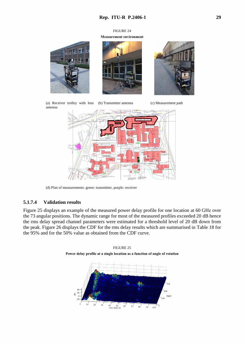
FIGURE 24
Measurement environment
(a) Receiver trolley with lens
antenna
(b) Transmitter antenna (c) Measurement path
(d) Plan of measurements: green: transmitter, purple: receiver
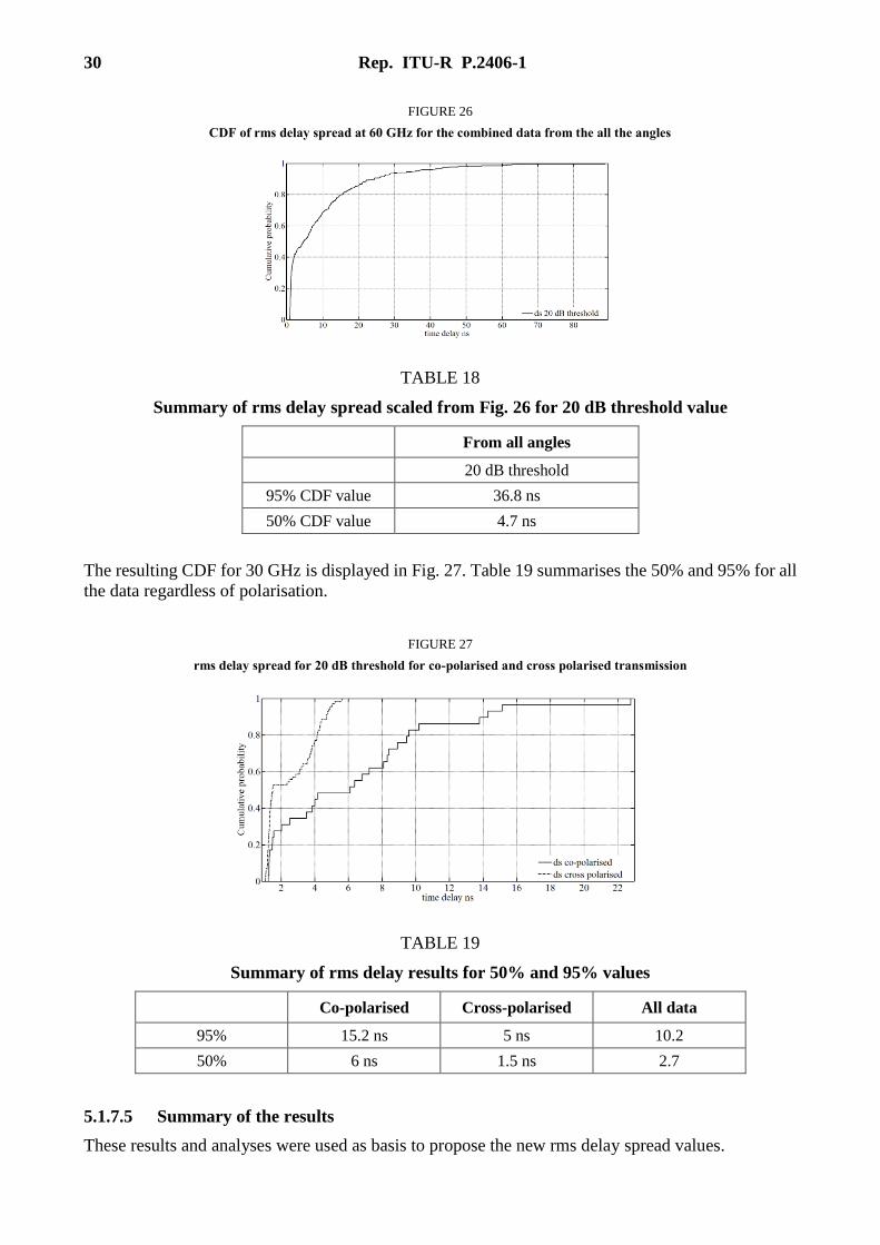
5.1.7.4 Validation results
Figure 25 displays an example of the measured power delay profile for one location at 60 GHz over
the 73 angular positions. The dynamic range for most of the measured profiles exceeded 20 dB hence
the rms delay spread channel parameters were estimated for a threshold level of 20 dB down from
the peak. Figure 26 displays the CDF for the rms delay results which are summarised in Table 18 for
the 95% and for the 50% value as obtained from the CDF curve.
FIGURE 25
Power delay profile at a single location as a function of angle of rotation
30 Rep. ITU-R P.2406-1
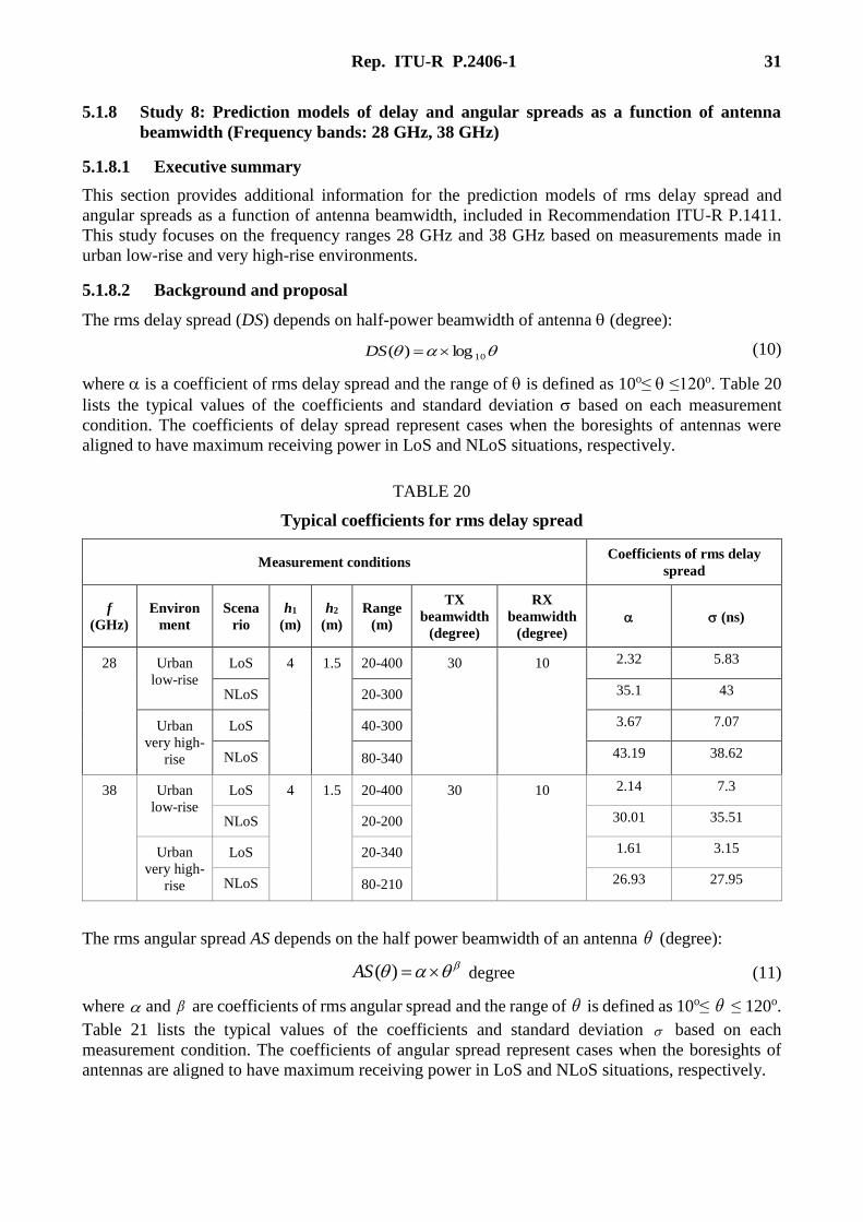
FIGURE 26
CDF of rms delay spread at 60 GHz for the combined data from the all the angles
TABLE 18
Summary of rms delay spread scaled from Fig. 26 for 20 dB threshold value
From all angles
20 dB threshold
95% CDF value 36.8 ns
50% CDF value 4.7 ns
The resulting CDF for 30 GHz is displayed in Fig. 27. Table 19 summarises the 50% and 95% for all
the data regardless of polarisation.
FIGURE 27
rms delay spread for 20 dB threshold for co-polarised and cross polarised transmission
TABLE 19
Summary of rms delay results for 50% and 95% values
Co-polarised Cross-polarised All data
95% 15.2 ns 5 ns 10.2
50% 6 ns 1.5 ns 2.7
5.1.7.5 Summary of the results
These results and analyses were used as basis to propose the new rms delay spread values.
Rep. ITU-R P.2406-1 31
5.1.8 Study 8: Prediction models of delay and angular spreads as a function of antenna
beamwidth (Frequency bands: 28 GHz, 38 GHz)
5.1.8.1 Executive summary
This section provides additional information for the prediction models of rms delay spread and
angular spreads as a function of antenna beamwidth, included in Recommendation ITU-R P.1411.
This study focuses on the frequency ranges 28 GHz and 38 GHz based on measurements made in
urban low-rise and very high-rise environments.
5.1.8.2 Background and proposal
The rms delay spread (DS) depends on half-power beamwidth of antenna (degree):
(10)
where is a coefficient of rms delay spread and the range of is defined as 10o≤ ≤120o. Table 20
lists the typical values of the coefficients and standard deviation based on each measurement
condition. The coefficients of delay spread represent cases when the boresights of antennas were
aligned to have maximum receiving power in LoS and NLoS situations, respectively.
TABLE 20
Typical coefficients for rms delay spread
Measurement conditions Coefficients of rms delay
spread
f
(GHz)
Environ
ment
Scena
rio
h1
(m)
h2
(m)
Range
(m)
TX
beamwidth
(degree)
RX
beamwidth
(degree) (ns)
28 Urban
low-rise
LoS 4 1.5 20-400 30 10 2.32 5.83
NLoS 20-300 35.1 43
Urban
very high-
rise
LoS 40-300 3.67 7.07
NLoS 80-340 43.19 38.62
38 Urban
low-rise
LoS 4 1.5 20-400 30 10 2.14 7.3
NLoS 20-200 30.01 35.51
Urban
very high-
rise
LoS 20-340 1.61 3.15
NLoS 80-210 26.93 27.95
The rms angular spread AS depends on the half power beamwidth of an antenna (degree):
degree (11)
where and are coefficients of rms angular spread and the range of is defined as 10o≤ ≤ 120o.
Table 21 lists the typical values of the coefficients and standard deviation based on each
measurement condition. The coefficients of angular spread represent cases when the boresights of
antennas are aligned to have maximum receiving power in LoS and NLoS situations, respectively.
10log)( DS
)(AS
32 Rep. ITU-R P.2406-1
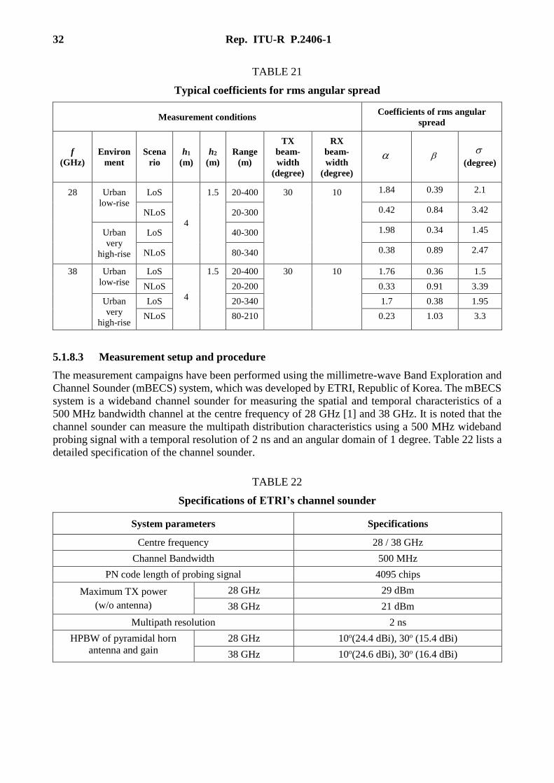
TABLE 21
Typical coefficients for rms angular spread
Measurement conditions Coefficients of rms angular
spread
f
(GHz)
Environ
ment
Scena
rio
h1
(m)
h2
(m)
Range
(m)
TX
beam-
width
(degree)
RX
beam-
width
(degree)
(degree)
28 Urban
low-rise
LoS
4
1.5 20-400 30 10 1.84 0.39 2.1
NLoS 20-300 0.42 0.84 3.42
Urban
very
high-rise
LoS 40-300 1.98 0.34 1.45
NLoS 80-340 0.38 0.89 2.47
38 Urban
low-rise
LoS
4
1.5 20-400 30 10 1.76 0.36 1.5
NLoS 20-200 0.33 0.91 3.39
Urban
very
high-rise
LoS 20-340 1.7 0.38 1.95
NLoS 80-210 0.23 1.03 3.3
5.1.8.3 Measurement setup and procedure
The measurement campaigns have been performed using the millimetre-wave Band Exploration and
Channel Sounder (mBECS) system, which was developed by ETRI, Republic of Korea. The mBECS
system is a wideband channel sounder for measuring the spatial and temporal characteristics of a
500 MHz bandwidth channel at the centre frequency of 28 GHz [1] and 38 GHz. It is noted that the
channel sounder can measure the multipath distribution characteristics using a 500 MHz wideband
probing signal with a temporal resolution of 2 ns and an angular domain of 1 degree. Table 22 lists a
detailed specification of the channel sounder.
TABLE 22
Specifications of ETRI’s channel sounder
System parameters Specifications
Centre frequency 28 / 38 GHz
Channel Bandwidth 500 MHz
PN code length of probing signal 4095 chips
Maximum TX power
(w/o antenna)
28 GHz 29 dBm
38 GHz 21 dBm
Multipath resolution 2 ns
HPBW of pyramidal horn
antenna and gain
28 GHz 10o(24.4 dBi), 30o (15.4 dBi)
38 GHz 10o(24.6 dBi), 30o (16.4 dBi)
Rep. ITU-R P.2406-1 33
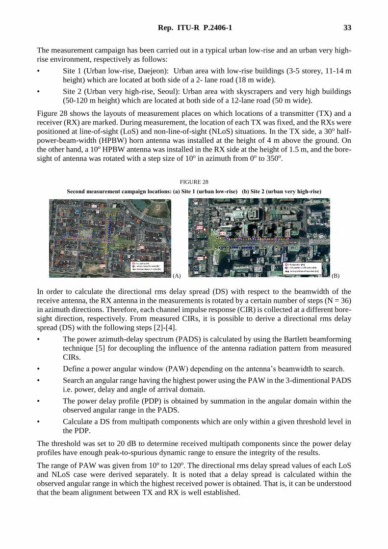
The measurement campaign has been carried out in a typical urban low-rise and an urban very high-
rise environment, respectively as follows:
• Site 1 (Urban low-rise, Daejeon): Urban area with low-rise buildings (3-5 storey, 11-14 m
height) which are located at both side of a 2- lane road (18 m wide).
• Site 2 (Urban very high-rise, Seoul): Urban area with skyscrapers and very high buildings
(50-120 m height) which are located at both side of a 12-lane road (50 m wide).
Figure 28 shows the layouts of measurement places on which locations of a transmitter (TX) and a
receiver (RX) are marked. During measurement, the location of each TX was fixed, and the RXs were
positioned at line-of-sight (LoS) and non-line-of-sight (NLoS) situations. In the TX side, a 30o half-
power-beam-width (HPBW) horn antenna was installed at the height of 4 m above the ground. On
the other hand, a 10o HPBW antenna was installed in the RX side at the height of 1.5 m, and the bore-
sight of antenna was rotated with a step size of 10o in azimuth from 0o to 350o.
FIGURE 28
Second measurement campaign locations: (a) Site 1 (urban low-rise) (b) Site 2 (urban very high-rise)
(A) (B)
In order to calculate the directional rms delay spread (DS) with respect to the beamwidth of the
receive antenna, the RX antenna in the measurements is rotated by a certain number of steps (N = 36)
in azimuth directions. Therefore, each channel impulse response (CIR) is collected at a different bore-
sight direction, respectively. From measured CIRs, it is possible to derive a directional rms delay
spread (DS) with the following steps [2]-[4].
• The power azimuth-delay spectrum (PADS) is calculated by using the Bartlett beamforming
technique [5] for decoupling the influence of the antenna radiation pattern from measured
CIRs.
• Define a power angular window (PAW) depending on the antenna’s beamwidth to search.
• Search an angular range having the highest power using the PAW in the 3-dimentional PADS
i.e. power, delay and angle of arrival domain.
• The power delay profile (PDP) is obtained by summation in the angular domain within the
observed angular range in the PADS.
• Calculate a DS from multipath components which are only within a given threshold level in
the PDP.
The threshold was set to 20 dB to determine received multipath components since the power delay
profiles have enough peak-to-spurious dynamic range to ensure the integrity of the results.
The range of PAW was given from 10o to 120o. The directional rms delay spread values of each LoS
and NLoS case were derived separately. It is noted that a delay spread is calculated within the
observed angular range in which the highest received power is obtained. That is, it can be understood
that the beam alignment between TX and RX is well established.

34 Rep. ITU-R P.2406-1
For the calculation of the directional rms angular spread (AS) with respect to the beamwidth of ther
receive antenna, the AS can be easily derived from the power azimuth spectrum (PAS). The PAS is
calculated from the PADS by summation in the delay domain [2]-[4]. To calculate the directional rms
AS, the threshold level was set to 20 dB.
5.1.8.4 Validation results
Figure 29 shows the DS curves obtained from measurement data at 28 and 38 GHz for the LoS and
NLoS case. To obtain the best fitted curves, mean values of rms DS for each beamwidth are utilized.
FIGURE 29
Measurement results of rms delay spread for 28 and 38 GHz: (a) LoS case (b) NLoS case
(A) (B)
Based on the measurement results, the following observations can be made:
– The DS has a strong dependency on the antenna beamwidth. The wider beamwidth has the
larger DS.
– The DSs in NLoS case is larger than the values of LoS case.
– These particular properties are very similar to the measurement results in a previous
contribution.
– In both LoS and NLoS cases, the curves of 28 GHz are higher than 38 GHz.
The rms AS with respect to with the standard deviation is given by equation (10).
Figure 30 shows the AS curves obtained from measurement data at 28 and 38 GHz for LoS and NLoS
cases. To obtain the best fitted curves, mean values of rms AS for each beamwidth are utilized.
FIGURE 30
Measurement results of rms angular spread for 28 and 38 GHz: (a) LoS case (b) NLoS case
(A) (B)
Rep. ITU-R P.2406-1 35
From measurement results, the following can be observed.
– The AS shows a strong dependency on the antenna beamwidth as similar to the DS. The
wider beamwidth of the antenna is the larger angular spread.
– Frequency dependency of AS is not clearly seen in both LoS and NLoS cases.
– At NLoS case, the angular spread monotonously increases from a narrow beam to a wider
beam.
– These particular properties are very similar to the measurement results in a previous
contribution.
The rms AS with respect to with the standard deviation is given by equation (11).
5.1.8.5 Summary of the results
This study presented prediction methods and coefficients for delay spread and angular spread
associated with antenna beamwidth based on additional measurement results in the 28 and 38 GHz
bands. The results and analyses show that both delay spread and angular spread have a strong
dependency on the antenna beamwidths.
5.1.8.6 References
[1] H.-K. Kwon et al., "Implementation and Performance Evaluation of mmWave Channel Sounding
System", in Proc. IEEE AP-S 2015, July 2015.
[2] M.-D. Kim et al., "Directional Multipath Propagation Characteristics based on 28 GHz Outdoor
Channel Measurements," in Proc. The European Conference on Antennas and Propagation (EuCAP),
April, 2016.
[3] M.-D. Kim et al., “Directional Delay Spread Characteristics based on Indoor Channel Measurements
at 28 GHz,” PIMRC 2015, pp. 505–509, Aug. 2015.
[4] M.-D. Kim et al., "Investigating the Effect of Antenna Beamwidth on Millimeter-wave Channel
Charaterization," accepted in 2016 The URSI Asia-Pacific Radio Science Conference (AP-RASC),
August, 2016.
[5] M. Bartlett, “Smoothing Periodograms from Time-Series with Continuous Spectra”, Nature, vol. 161,
1948.
5.1.9 Study 9: Cross-polarization discrimination (Frequency bands: 51-57, 67-73 GHz)
5.1.9.1 Executive summary
This section provides additional information related to the cross-polarization discrimination values
included in Recommendation ITU-R P.1411 for the 51-57 GHz and 67-67 GHz bands.
5.1.9.2 Background and proposal
In the millimetre band the measured cross-polarization characteristics for the bands 51-57 GHz and
67-73 GHz in a low rise urban environment has a median value of 16 dB for the LoS component with
3 dB variance and 9 dB for NLoS paths with a 6 dB variance.
5.1.9.3 Measurement setup and procedure
To study the radio channel in the millimetre wave band, a custom designed radio channel sounder
capable of measuring with two transmit and two receive antennas has been designed [1] and used for
measurements in an outdoor environment in a low rise urban environment with the transmit antenna
height being either below the roof top at 3 m or above the roof tops at 18.2 m and a receiver antenna
height of 1.6 m. Horn antennas were used at the receiver with a beam width (18.4o in the E plane and
19.7o in the H plane at 50 GHz with 19 dB gain and 14.4o in the E plane and 15.4o in the H plane with
36 Rep. ITU-R P.2406-1
21 dB gain at 67.5 GHz). At the transmitter two horn antennas were used and these have beam widths
(56.3o in the E plane and 51.4o in the H plane with 11 dB gain at 50 GHz and 40o in the E plane and
38o in the H plane with 13.5 dB gain at 67.5 GHz). To perform dual polarisation measurements, a
twist was used at one of the transmit channels and another at one of the receive channels. To enable
LoS, NLoS and the synthesis of non-directional propagation, the receiver was mounted on a turntable
which was rotated in 5 degree steps. The measurements were performed with a 6 GHz bandwidth at
305 Hz waveform repetition frequency and data were acquired over 1 second for each angle of
rotation. Measurements were performed in two frequency bands: 51-57 GHz and 67-73 GHz along a
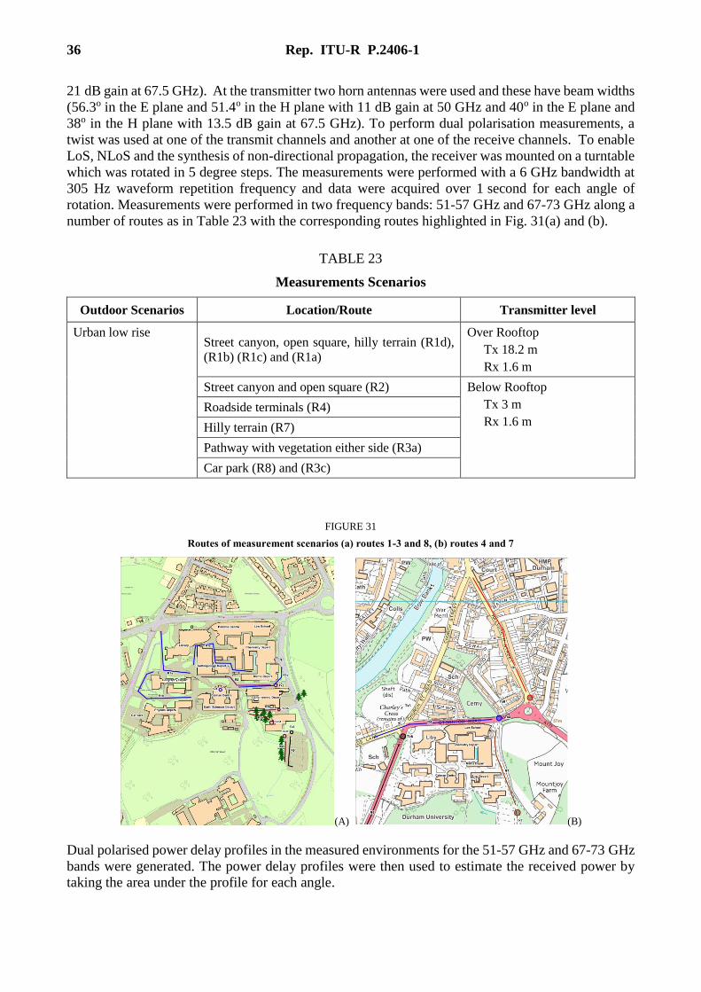
number of routes as in Table 23 with the corresponding routes highlighted in Fig. 31(a) and (b).
TABLE 23
Measurements Scenarios
Outdoor Scenarios Location/Route Transmitter level
Urban low rise Street canyon, open square, hilly terrain (R1d),
(R1b) (R1c) and (R1a)
Over Rooftop
Tx 18.2 m
Rx 1.6 m
Street canyon and open square (R2) Below Rooftop
Tx 3 m
Rx 1.6 m Roadside terminals (R4)
Hilly terrain (R7)
Pathway with vegetation either side (R3a)
Car park (R8) and (R3c)
FIGURE 31
Routes of measurement scenarios (a) routes 1-3 and 8, (b) routes 4 and 7
(A) (B)
Dual polarised power delay profiles in the measured environments for the 51-57 GHz and 67-73 GHz
bands were generated. The power delay profiles were then used to estimate the received power by
taking the area under the profile for each angle.

Rep. ITU-R P.2406-1 37
Following full calibration of the data, the received power was then used to estimate the transmission
loss for the following antenna beam widths:
1 Strongest beam: The maximum received power representing the main beam of the receive
antenna. When unobstructed by vegetation or buildings it represents the LoS.
2 40omain beam power: The received power for a 40o beam width around the maximum
received power.
3 NLoS: The sum of the received power from the remaining angles outside the 40o main beam.
4 360o (omni-directional): The sum from all the azimuthal angles.
Since the antenna azimuthal beam width is larger than the rotational angular step, the transmission
loss was adjusted for the additional antenna gain due to the overlap of the beam.
These were then used to estimate transmission loss coefficients for the different measurement
scenarios. The scenario in Fig. 32 corresponds to route 2, which combines non-line of sight around
the corner of the building and locations where the receiver antenna when pointed toward the
transmitter was in the line of sight. For the LoS component transmission loss estimation, the NLoS
data were filtered out.
FIGURE 32
Measurement environment for route 2 (street canyon and open square) indicated by the blue line
5.1.9.4 Validation results
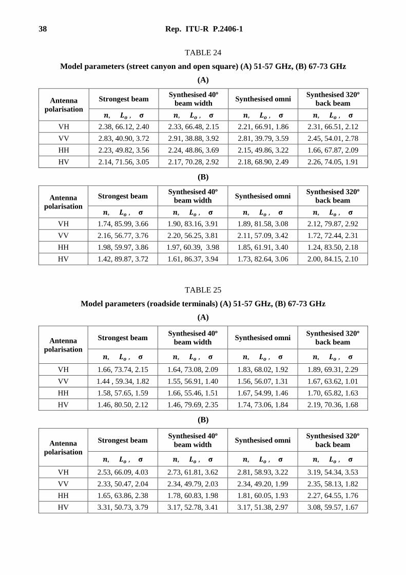
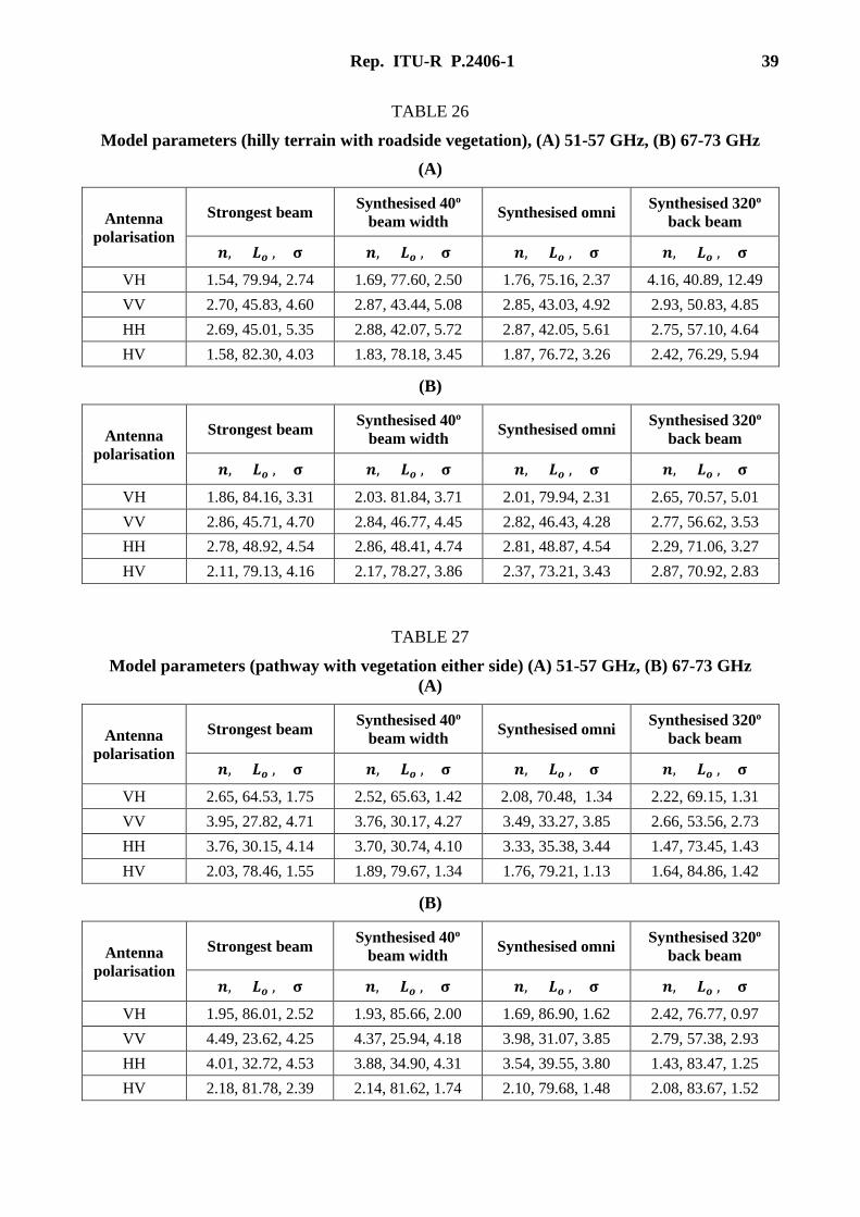
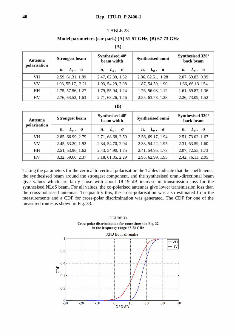
Tables 24 to 28 give a summary of the results of transmission loss parameters for the dual polarised
transmissions for the 51-56 GHz and 67-73 GHz frequency bands using equation (12) which
corresponds to equation (12) in Recommendation ITU-R P.1411-8 with the additional term σ which
represents the standard deviation of the fit, where n represents the transmission loss coefficient, 𝐿𝑜
is the transmission loss at a reference distance, 𝑑𝑜 = 1
𝑃𝐿(𝑑) = 𝐿𝑜 + 10𝑛𝑙𝑜𝑔10 (𝑑
𝑑𝑜) + 𝐿𝑔𝑎𝑠 + 𝐿𝑟𝑎𝑖𝑛 + σ 𝑑𝐵 (12)
38 Rep. ITU-R P.2406-1
TABLE 24
Model parameters (street canyon and open square) (A) 51-57 GHz, (B) 67-73 GHz
(A)
Antenna
polarisation
Strongest beam Synthesised 40o
beam width Synthesised omni
Synthesised 320o
back beam
𝒏, 𝑳𝒐 , 𝛔 𝒏, 𝑳𝒐 , 𝛔 𝒏, 𝑳𝒐 , 𝛔 𝒏, 𝑳𝒐 , 𝛔
VH 2.38, 66.12, 2.40 2.33, 66.48, 2.15 2.21, 66.91, 1.86 2.31, 66.51, 2.12
VV 2.83, 40.90, 3.72 2.91, 38.88, 3.92 2.81, 39.79, 3.59 2.45, 54.01, 2.78
HH 2.23, 49.82, 3.56 2.24, 48.86, 3.69 2.15, 49.86, 3.22 1.66, 67.87, 2.09
HV 2.14, 71.56, 3.05 2.17, 70.28, 2.92 2.18, 68.90, 2.49 2.26, 74.05, 1.91
(B)
Antenna
polarisation
Strongest beam Synthesised 40o
beam width Synthesised omni
Synthesised 320o
back beam
𝒏, 𝑳𝒐 , 𝛔 𝒏, 𝑳𝒐 , 𝛔 𝒏, 𝑳𝒐 , 𝛔 𝒏, 𝑳𝒐 , 𝛔
VH 1.74, 85.99, 3.66 1.90, 83.16, 3.91 1.89, 81.58, 3.08 2.12, 79.87, 2.92
VV 2.16, 56.77, 3.76 2.20, 56.25, 3.81 2.11, 57.09, 3.42 1.72, 72.44, 2.31
HH 1.98, 59.97, 3.86 1.97, 60.39, 3.98 1.85, 61.91, 3.40 1.24, 83.50, 2.18
HV 1.42, 89.87, 3.72 1.61, 86.37, 3.94 1.73, 82.64, 3.06 2.00, 84.15, 2.10
TABLE 25
Model parameters (roadside terminals) (A) 51-57 GHz, (B) 67-73 GHz
(A)
Antenna
polarisation
Strongest beam Synthesised 40o
beam width Synthesised omni
Synthesised 320o
back beam
𝒏, 𝑳𝒐 , 𝛔 𝒏, 𝑳𝒐 , 𝛔 𝒏, 𝑳𝒐 , 𝛔 𝒏, 𝑳𝒐 , 𝛔
VH 1.66, 73.74, 2.15 1.64, 73.08, 2.09 1.83, 68.02, 1.92 1.89, 69.31, 2.29
VV 1.44 , 59.34, 1.82 1.55, 56.91, 1.40 1.56, 56.07, 1.31 1.67, 63.62, 1.01
HH 1.58, 57.65, 1.59 1.66, 55.46, 1.51 1.67, 54.99, 1.46 1.70, 65.82, 1.63
HV 1.46, 80.50, 2.12 1.46, 79.69, 2.35 1.74, 73.06, 1.84 2.19, 70.36, 1.68
(B)
Antenna
polarisation
Strongest beam Synthesised 40o
beam width Synthesised omni
Synthesised 320o
back beam
𝒏, 𝑳𝒐 , 𝛔 𝒏, 𝑳𝒐 , 𝛔 𝒏, 𝑳𝒐 , 𝛔 𝒏, 𝑳𝒐 , 𝛔
VH 2.53, 66.09, 4.03 2.73, 61.81, 3.62 2.81, 58.93, 3.22 3.19, 54.34, 3.53
VV 2.33, 50.47, 2.04 2.34, 49.79, 2.03 2.34, 49.20, 1.99 2.35, 58.13, 1.82
HH 1.65, 63.86, 2.38 1.78, 60.83, 1.98 1.81, 60.05, 1.93 2.27, 64.55, 1.76
HV 3.31, 50.73, 3.79 3.17, 52.78, 3.41 3.17, 51.38, 2.97 3.08, 59.57, 1.67
Rep. ITU-R P.2406-1 39
TABLE 26
Model parameters (hilly terrain with roadside vegetation), (A) 51-57 GHz, (B) 67-73 GHz
(A)
Antenna
polarisation
Strongest beam Synthesised 40o
beam width Synthesised omni
Synthesised 320o
back beam
𝒏, 𝑳𝒐 , 𝛔 𝒏, 𝑳𝒐 , 𝛔 𝒏, 𝑳𝒐 , 𝛔 𝒏, 𝑳𝒐 , 𝛔
VH 1.54, 79.94, 2.74 1.69, 77.60, 2.50 1.76, 75.16, 2.37 4.16, 40.89, 12.49
VV 2.70, 45.83, 4.60 2.87, 43.44, 5.08 2.85, 43.03, 4.92 2.93, 50.83, 4.85
HH 2.69, 45.01, 5.35 2.88, 42.07, 5.72 2.87, 42.05, 5.61 2.75, 57.10, 4.64
HV 1.58, 82.30, 4.03 1.83, 78.18, 3.45 1.87, 76.72, 3.26 2.42, 76.29, 5.94
(B)
Antenna
polarisation
Strongest beam Synthesised 40o
beam width Synthesised omni
Synthesised 320o
back beam
𝒏, 𝑳𝒐 , 𝛔 𝒏, 𝑳𝒐 , 𝛔 𝒏, 𝑳𝒐 , 𝛔 𝒏, 𝑳𝒐 , 𝛔
VH 1.86, 84.16, 3.31 2.03. 81.84, 3.71 2.01, 79.94, 2.31 2.65, 70.57, 5.01
VV 2.86, 45.71, 4.70 2.84, 46.77, 4.45 2.82, 46.43, 4.28 2.77, 56.62, 3.53
HH 2.78, 48.92, 4.54 2.86, 48.41, 4.74 2.81, 48.87, 4.54 2.29, 71.06, 3.27
HV 2.11, 79.13, 4.16 2.17, 78.27, 3.86 2.37, 73.21, 3.43 2.87, 70.92, 2.83
TABLE 27
Model parameters (pathway with vegetation either side) (A) 51-57 GHz, (B) 67-73 GHz
(A)
Antenna
polarisation
Strongest beam Synthesised 40o
beam width Synthesised omni
Synthesised 320o
back beam
𝒏, 𝑳𝒐 , 𝛔 𝒏, 𝑳𝒐 , 𝛔 𝒏, 𝑳𝒐 , 𝛔 𝒏, 𝑳𝒐 , 𝛔
VH 2.65, 64.53, 1.75 2.52, 65.63, 1.42 2.08, 70.48, 1.34 2.22, 69.15, 1.31
VV 3.95, 27.82, 4.71 3.76, 30.17, 4.27 3.49, 33.27, 3.85 2.66, 53.56, 2.73
HH 3.76, 30.15, 4.14 3.70, 30.74, 4.10 3.33, 35.38, 3.44 1.47, 73.45, 1.43
HV 2.03, 78.46, 1.55 1.89, 79.67, 1.34 1.76, 79.21, 1.13 1.64, 84.86, 1.42
(B)
Antenna
polarisation
Strongest beam Synthesised 40o
beam width Synthesised omni
Synthesised 320o
back beam
𝒏, 𝑳𝒐 , 𝛔 𝒏, 𝑳𝒐 , 𝛔 𝒏, 𝑳𝒐 , 𝛔 𝒏, 𝑳𝒐 , 𝛔
VH 1.95, 86.01, 2.52 1.93, 85.66, 2.00 1.69, 86.90, 1.62 2.42, 76.77, 0.97
VV 4.49, 23.62, 4.25 4.37, 25.94, 4.18 3.98, 31.07, 3.85 2.79, 57.38, 2.93
HH 4.01, 32.72, 4.53 3.88, 34.90, 4.31 3.54, 39.55, 3.80 1.43, 83.47, 1.25
HV 2.18, 81.78, 2.39 2.14, 81.62, 1.74 2.10, 79.68, 1.48 2.08, 83.67, 1.52
40 Rep. ITU-R P.2406-1
TABLE 28
Model parameters (car park) (A) 51-57 GHz, (B) 67-73 GHz
(A)
Antenna
polarisation
Strongest beam Synthesised 40o
beam width Synthesised omni
Synthesised 320o
back beam
𝒏, 𝑳𝒐 , 𝛔 𝒏, 𝑳𝒐 , 𝛔 𝒏, 𝑳𝒐 , 𝛔 𝒏, 𝑳𝒐 , 𝛔
VH 2.59, 61.31, 1.89 2.47, 62.39, 1.52 2.36, 62.51, 1.28 2.07, 69.83, 0.99
VV 1.93, 55.17, 2.21 1.93, 54.29, 2.08 1.87, 54.50, 1.90 1.66, 66.13 1.54
HH 1.75, 57.56, 1.27 1.79, 55.94, 1.24 1.76, 56.08, 1.12 1.61, 69.87, 1.36
HV 2.76, 63.52, 1.63 2.71, 63.26, 1.46 2.55, 63.78, 1.28 2.26, 73.09, 1.52
(B)
Antenna
polarisation
Strongest beam Synthesised 40o
beam width Synthesised omni
Synthesised 320o
back beam
𝒏, 𝑳𝒐 , 𝛔 𝒏, 𝑳𝒐 , 𝛔 𝒏, 𝑳𝒐 , 𝛔 𝒏, 𝑳𝒐 , 𝛔
VH 2.85, 66.99, 2.79 2.71, 68.68, 2.50 2.56, 69.17, 1.94 2.51, 73.02, 1.67
VV 2.45, 53.20, 1.92 2.34, 54.70, 2.04 2.33, 54.22, 1.95 2.31, 63.59, 1.60
HH 2.51, 53.96, 1.62 2.43, 54.90, 1.75 2.41, 54.95, 1.73 2.07, 72.55, 1.73
HV 3.32, 59.60, 2.37 3.18, 61.35, 2.29 2.95, 62.99, 1.95 2.42, 76.13, 2.05
Taking the parameters for the vertical to vertical polarisation the Tables indicate that the coefficients,
the synthesised beam around the strongest component, and the synthesised omni-directional beam
give values which are fairly close with about 18-19 dB increase in transmission loss for the
synthesised NLoS beam. For all values, the co-polarised antennas give lower transmission loss than
the cross-polarised antennas. To quantify this, the cross-polarisation was also estimated from the
measurements and a CDF for cross-polar discrimination was generated. The CDF for one of the
measured routes is shown in Fig. 33.
FIGURE 33
Cross polar discrimination for route shown in Fig. 32
in the frequency range 67-73 GHz
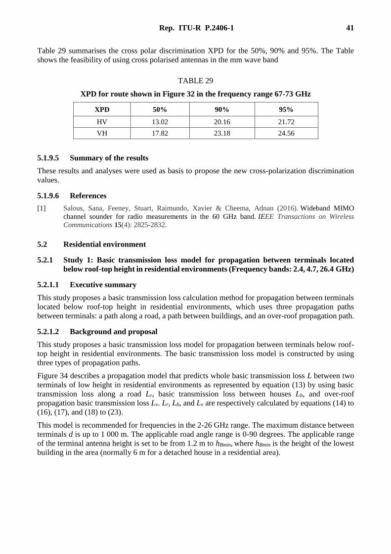
Rep. ITU-R P.2406-1 41
Table 29 summarises the cross polar discrimination XPD for the 50%, 90% and 95%. The Table
shows the feasibility of using cross polarised antennas in the mm wave band
TABLE 29
XPD for route shown in Figure 32 in the frequency range 67-73 GHz
XPD 50% 90% 95%
HV 13.02 20.16 21.72
VH 17.82 23.18 24.56
5.1.9.5 Summary of the results
These results and analyses were used as basis to propose the new cross-polarization discrimination
values.
5.1.9.6 References
[1] Salous, Sana, Feeney, Stuart, Raimundo, Xavier & Cheema, Adnan (2016). Wideband MIMO
channel sounder for radio measurements in the 60 GHz band. IEEE Transactions on Wireless
Communications 15(4): 2825-2832.
5.2 Residential environment
5.2.1 Study 1: Basic transmission loss model for propagation between terminals located
below roof-top height in residential environments (Frequency bands: 2.4, 4.7, 26.4 GHz)
5.2.1.1 Executive summary
This study proposes a basic transmission loss calculation method for propagation between terminals
located below roof-top height in residential environments, which uses three propagation paths
between terminals: a path along a road, a path between buildings, and an over-roof propagation path.
5.2.1.2 Background and proposal
This study proposes a basic transmission loss model for propagation between terminals below roof-
top height in residential environments. The basic transmission loss model is constructed by using
three types of propagation paths.
Figure 34 describes a propagation model that predicts whole basic transmission loss L between two
terminals of low height in residential environments as represented by equation (13) by using basic
transmission loss along a road Lr, basic transmission loss between houses Lb, and over-roof
propagation basic transmission loss Lv. Lr, Lb, and Lv are respectively calculated by equations (14) to
(16), (17), and (18) to (23).
This model is recommended for frequencies in the 2-26 GHz range. The maximum distance between
terminals d is up to 1 000 m. The applicable road angle range is 0-90 degrees. The applicable range
of the terminal antenna height is set to be from 1.2 m to hBmin, where hBmin is the height of the lowest
building in the area (normally 6 m for a detached house in a residential area).

42 Rep. ITU-R P.2406-1
FIGURE 34
Propagation model for paths between terminals located below roof-top height
(13)
(14)
(15)
(16)
(17)
(18)
(19)
(20)
(21)
(22)
(23)
The relevant parameters for this model are:
d: distance between two terminals (m);
: wavelength (m);
f: frequency (GHz);
i: road angle of i-th corner (degrees);
x1i: road distance from transmitter to i-th corner (m);
x2i: road distance from i-th corner to receiver (m);
Tx
Rx
Lr
Lb
Lv
)10/110/110/1log(10)10/()10/()10/( vbr LLL
L
)(
)(
cornerafterL
cornerbeforeLL
rac
rbc
r
)/4log(20 dLrbc
iii
i
irbcrac xxfLL 21
51072.3exp1)1.6)log(97.0)log(18.7(
76.5)log(88.6)/log(6.30)/4log(20 fRddLb
cv LLLdL 21)/4log(20
1.01)1.0(log209.6 1
2
11 vvL
1.01)1.0(log209.6 2
2
22 vvL
bahhv TxbTx
1121
cbhhv RxbRx
1122
)(
))((log10
cbab
cbbaLc

Rep. ITU-R P.2406-1 43
R: mean visible distance (m);
hbTx: height of nearest building from transmitter in receiver direction (m);
hbRx: height of nearest building from receiver in transmitter direction (m);
hTx: transmitter antenna height (m);
hRx: receiver antenna height (m);
a: distance between transmitter and nearest building from transmitter (m);
b: distance between nearest buildings from transmitter and receiver (m);
c: distance between receiver and nearest building from receiver (m).
5.1.1.2 Measurement setup and procedure
The measurement parameters are summarized in Table 30.
TABLE 30
Measurement parameters
Frequency (GHz) 2.1975, 4.703, 26.365
Tx antenna height (m) 2.5
Rx antenna height (m) 2.5
Antenna type Omni-directional (Tx and Rx)
Measurement frequencies were 2.1975, 4.703, and 26.365 GHz. To measure basic transmission loss
characteristics below house-roof height, the heights of the Tx and Rx antennas were set at 2.5 m.
Omni-directional antennas were used at Tx and Rx.
Tx was set at the roadside, and Rx was set on the measurement vehicle. Figure 35 shows the
measurement environment and routes. The average building height is 6.7 m, and the mean visible
distance R is 67 m, which were calculated using the building database. The measurement area has
many detached houses and is a typical residential environment. The measurement route has four
corners (the black dashed lines in Fig. 35) and can be separated to five parts, A to E.
The corners from A to B and from D to E are right-angle corners, and so, the road angles are
90 degrees at these corners. The corners from B to C and from C to D are gently curved, and the LoS
between Tx and Rx is shielded. Both road angles of these gently curved corners are 10 degrees. Part
C is LoS, and the other parts are NLoS. The measurement data were obtained by running the
measurement vehicle along the route from part A to E.

44 Rep. ITU-R P.2406-1
FIGURE 35
Measurement environment and routes
5.2.1.4 Validation results
Figure 36 compares the predicted total basic transmission losses calculated with the proposed model
and the measured results. The parts of the measurement route are also represented in the Figure. This
Figure shows that the predictions and measurements have good agreement over the whole route.
Further analyses show that the path along the road is dominant on almost the whole route of parts B,
C and D. On the other hand, in parts A and E, the path between buildings become dominant, and the
over-rooftop path as well as the path along the road becomes strong. Also, the effects of the path
between buildings and the over-rooftop path decrease with increasing frequency, and the path along
road become dominant on the whole measurement route.
Figure 37 shows the prediction error calculated from the measured basic transmission losses and
predictions. The error values lie between −20 dB and 20 dB for the areas where a single path type is
dominant. The root mean square values of the prediction error are 5.5 dB, 5.0 dB, and 5.5 dB at
2.2 GHz, 4.7 GHz, and 26 GHz, respectively. These results show that the model can predict the actual
basic transmission loss accurately in the environment.
A
B
C
D
E
Tx
100m
Running
direction
Copyright(c) 2015 ZENRIN Co.,LTD. (Z14BJ第294号)
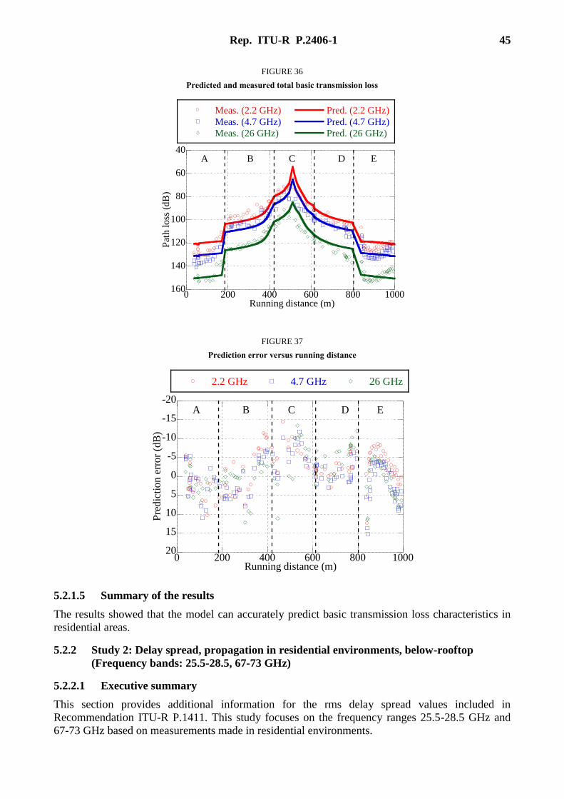
Rep. ITU-R P.2406-1 45
FIGURE 36
Predicted and measured total basic transmission loss
FIGURE 37
Prediction error versus running distance
5.2.1.5 Summary of the results
The results showed that the model can accurately predict basic transmission loss characteristics in
residential areas.
5.2.2 Study 2: Delay spread, propagation in residential environments, below-rooftop
(Frequency bands: 25.5-28.5, 67-73 GHz)
5.2.2.1 Executive summary
This section provides additional information for the rms delay spread values included in
Recommendation ITU-R P.1411. This study focuses on the frequency ranges 25.5-28.5 GHz and
67-73 GHz based on measurements made in residential environments.
40
60
80
100
120
140
1600 200 400 600 800 1000
Meas. (2.2 GHz)
Meas. (4.7 GHz)
Meas. (26 GHz)
Pred. (2.2 GHz)
Pred. (4.7 GHz)
Pred. (26 GHz)
Pat
h l
oss
(d
B)
Running distance (m)
A B C D E
-20
-15
-10
-5
0
5
10
15
200 200 400 600 800 1000
2.2 GHz 4.7 GHz 26 GHz
Pre
dic
tion
err
or
(dB
)
Running distance (m)
A B C D E

46 Rep. ITU-R P.2406-1
5.2.2.2 Background and proposal
Table 31 shows the proposed rms delay spread values.
TABLE 31
Rms delay spread values for 25.5-28.5 GHz and 67-73 GHz
Measurement conditions
rms delay
spread
(ns)
Area Scena
rio
f
(GHz)
h1
(m)
h2
(m)
Range
(m)
TX
beam-
width
(degree)
RX
beam-
width
(degree)
Time
delay
resoluti
on (ns)
Polariza
tion 50% 95%
Resid
ential NLoS
25.5-
28.5 3 1.6 37-167 33 Omni 0.5
VV 5.3 13.6
HV 9.1 15.5
67-73 3 1.6 37-167 40 Omni 0.5 VV 7.4 15.4
5.2.2.3 Measurement setup and procedure
Measurements were performed with dual polarised antennas at the transmitter and an omni-
directional antenna at the receiver with vertical polarisation. At the transmitter two horn antennas
with beam widths (40o in the E-plane and 38o in the H-plane) were used in the 67-73 GHz band with
a twist at one of the transmit channels. In addition, a new set of dual polarised transmitters and two
receivers were designed and implemented to perform measurements in the 25.5-28.5 GHz band. The
transmit antenna has a 3 dB beam width of ~36o in the H-plane and 33o in the E-plane and the receive
antenna was omni-directional. The measured environments include above rooftop and below roof top
in both residential and low rise urban environments. The measurements were performed in both line
of sight and non-line of sight where the transmitter was placed around the corner of a street. The data
were systematically collected by moving the receiver trolley over consecutive 1 m intervals and the
power delay profiles were then obtained by dividing the 1 m data into five sections. The data were
analysed with 2 GHz bandwidth to give a 0.5 ns time delay resolution and the power delay profiles
were used to estimate the rms delay spread in the two frequency bands for 20 dB threshold using the
method defined in Recommendation ITU-R P.1407. Figure 38 shows the measured residential
environment.
FIGURE 38
View of the measured environment (residential street)
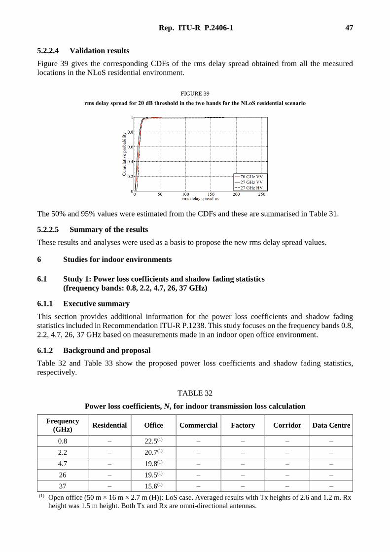
Rep. ITU-R P.2406-1 47
5.2.2.4 Validation results
Figure 39 gives the corresponding CDFs of the rms delay spread obtained from all the measured
locations in the NLoS residential environment.
FIGURE 39
rms delay spread for 20 dB threshold in the two bands for the NLoS residential scenario
The 50% and 95% values were estimated from the CDFs and these are summarised in Table 31.
5.2.2.5 Summary of the results
These results and analyses were used as a basis to propose the new rms delay spread values.
6 Studies for indoor environments
6.1 Study 1: Power loss coefficients and shadow fading statistics
(frequency bands: 0.8, 2.2, 4.7, 26, 37 GHz)
6.1.1 Executive summary
This section provides additional information for the power loss coefficients and shadow fading
statistics included in Recommendation ITU-R P.1238. This study focuses on the frequency bands 0.8,
2.2, 4.7, 26, 37 GHz based on measurements made in an indoor open office environment.
6.1.2 Background and proposal
Table 32 and Table 33 show the proposed power loss coefficients and shadow fading statistics,
respectively.
TABLE 32
Power loss coefficients, N, for indoor transmission loss calculation
Frequency
(GHz) Residential Office Commercial Factory Corridor Data Centre
0.8 – 22.5(1) – – – –
2.2 – 20.7(1) – – – –
4.7 – 19.8(1) – – – –
26 – 19.5(1) – – – –
37 – 15.6(1) – – – –
(1) Open office (50 m × 16 m × 2.7 m (H)): LoS case. Averaged results with Tx heights of 2.6 and 1.2 m. Rx
height was 1.5 m height. Both Tx and Rx are omni-directional antennas.

48 Rep. ITU-R P.2406-1
TABLE 33
Shadow fading statistics, standard deviation (dB),
for indoor transmission loss calculation
Frequency
(GHz) Residential Office Commercial
0.8 – 3.4 –
2.2 – 2.3 –
4.7 – 2.7 –
26 – 2.8 –
37 – 2.4 –
6.1.3 Measurement setup and procedure
Figure 40 shows the measurement environment and measurement parameters summarized in
Table 34. The measurement environment was a large office environment (50 m width × 16 m depth
× 2.7 m above-floor height). Transmitter (Tx) antennas were placed in two locations (Tx1/3 and Tx2).
Tx 1/3 were set near the centre of the room and Tx2 was placed near the edge of the room as shown
in Fig. 40. For Tx1 and Tx2, the height of the Tx antennas was 2.6 m above the floor (0.1 m from the
ceiling), and the antenna height of Tx3 was 1.2 m above the floor. Receive (Rx) antennas with a
height of 1.5 m above the floor (1.2 m from the ceiling) were set on a push car. When the Tx antenna
height was 2.6 m (Tx1 and Tx2), the measurements were taken in LoS between Tx and Rx antennas.
For an antenna height of 1.2 m (Tx3), obstacles on the desk and partitions in the room caused quasi
LoS because of blockages between Tx and Rx. The received power was measured by moving the
push car as shown along the red line in Fig. 40. Five measurement frequencies were used, including
high frequency bands above 6 GHz (0.8, 2.2, 4.7, 26.4, 37.1 GHz). A continuous wave was used at
all five frequencies. Both the Tx and Rx antennas’ radiation patterns were omni-directional in the
horizontal plane with a 60-degree half-power beam width in the vertical plane. The basic transmission
loss was obtained by subtracting gains and losses of the measurement setup after calibration. In order
to exclude the effects of fast fading, median values were obtained at 1-meter intervals.
FIGURE 40
Measurement environment
49.8 m
16m
4m
45m
Tx2
Tx1
Tx3
Rx route
3.5m
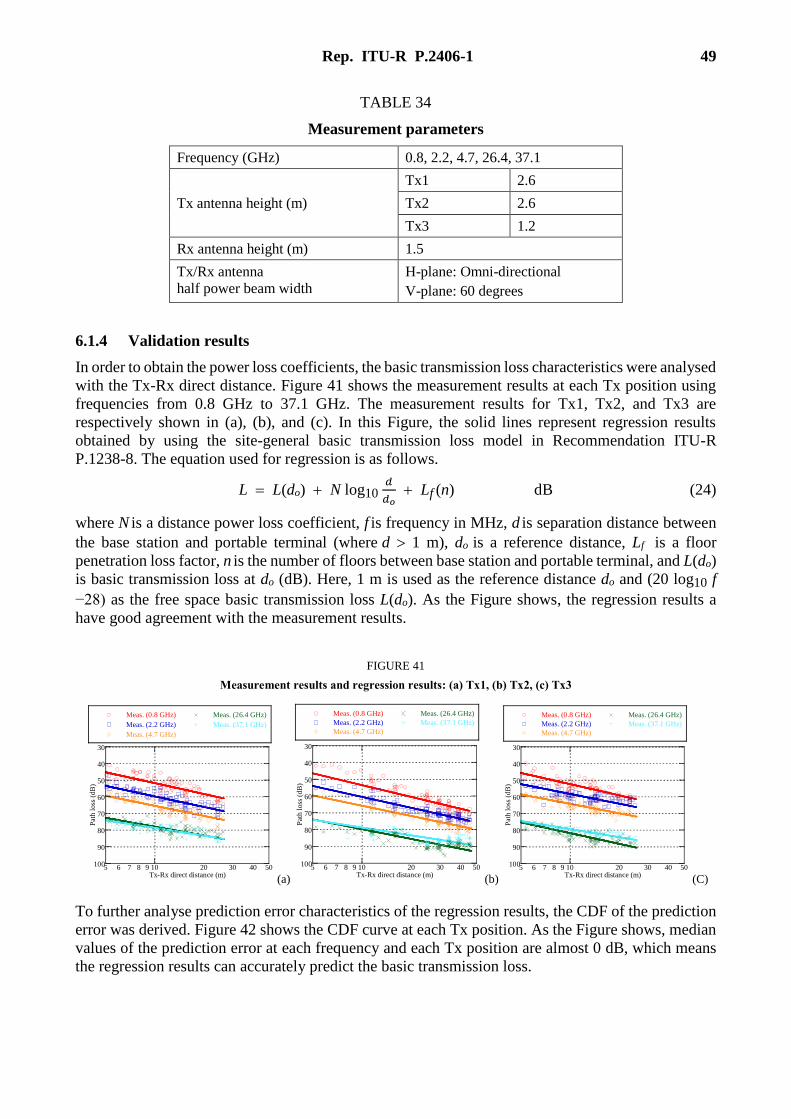
Rep. ITU-R P.2406-1 49
TABLE 34
Measurement parameters
Frequency (GHz) 0.8, 2.2, 4.7, 26.4, 37.1
Tx antenna height (m)
Tx1 2.6
Tx2 2.6
Tx3 1.2
Rx antenna height (m) 1.5
Tx/Rx antenna
half power beam width
H-plane: Omni-directional
V-plane: 60 degrees
6.1.4 Validation results
In order to obtain the power loss coefficients, the basic transmission loss characteristics were analysed
with the Tx-Rx direct distance. Figure 41 shows the measurement results at each Tx position using
frequencies from 0.8 GHz to 37.1 GHz. The measurement results for Tx1, Tx2, and Tx3 are
respectively shown in (a), (b), and (c). In this Figure, the solid lines represent regression results
obtained by using the site-general basic transmission loss model in Recommendation ITU-R
P.1238-8. The equation used for regression is as follows.
L L(do) N log10 𝑑
𝑑𝑜 Lf (n) dB (24)
where N is a distance power loss coefficient, f is frequency in MHz, d is separation distance between
the base station and portable terminal (where d 1 m), do is a reference distance, Lf is a floor
penetration loss factor, n is the number of floors between base station and portable terminal, and L(do)
is basic transmission loss at do (dB). Here, 1 m is used as the reference distance do and (20 log10 f
−28) as the free space basic transmission loss L(do). As the Figure shows, the regression results a
have good agreement with the measurement results.
FIGURE 41
Measurement results and regression results: (a) Tx1, (b) Tx2, (c) Tx3
(a) (b) (C)
To further analyse prediction error characteristics of the regression results, the CDF of the prediction
error was derived. Figure 42 shows the CDF curve at each Tx position. As the Figure shows, median
values of the prediction error at each frequency and each Tx position are almost 0 dB, which means
the regression results can accurately predict the basic transmission loss.
30
40
50
60
70
80
90
1005 6 7 8 9 10 20 30 40 50
Meas. (0.8 GHz)
Meas. (2.2 GHz)
Meas. (4.7 GHz)
Meas. (26.4 GHz)
Meas. (37.1 GHz)
Pat
h l
oss
(dB
)
Tx-Rx direct distance (m)
30
40
50
60
70
80
90
1005 6 7 8 9 10 20 30 40 50
Meas. (0.8 GHz)
Meas. (2.2 GHz)
Meas. (4.7 GHz)
Meas. (26.4 GHz)
Meas. (37.1 GHz)
Pat
h l
oss
(dB
)
Tx-Rx direct distance (m)
30
40
50
60
70
80
90
1005 6 7 8 9 10 20 30 40 50
Meas. (0.8 GHz)
Meas. (2.2 GHz)
Meas. (4.7 GHz)
Meas. (26.4 GHz)
Meas. (37.1 GHz)
Pat
h l
oss
(dB
)
Tx-Rx direct distance (m)
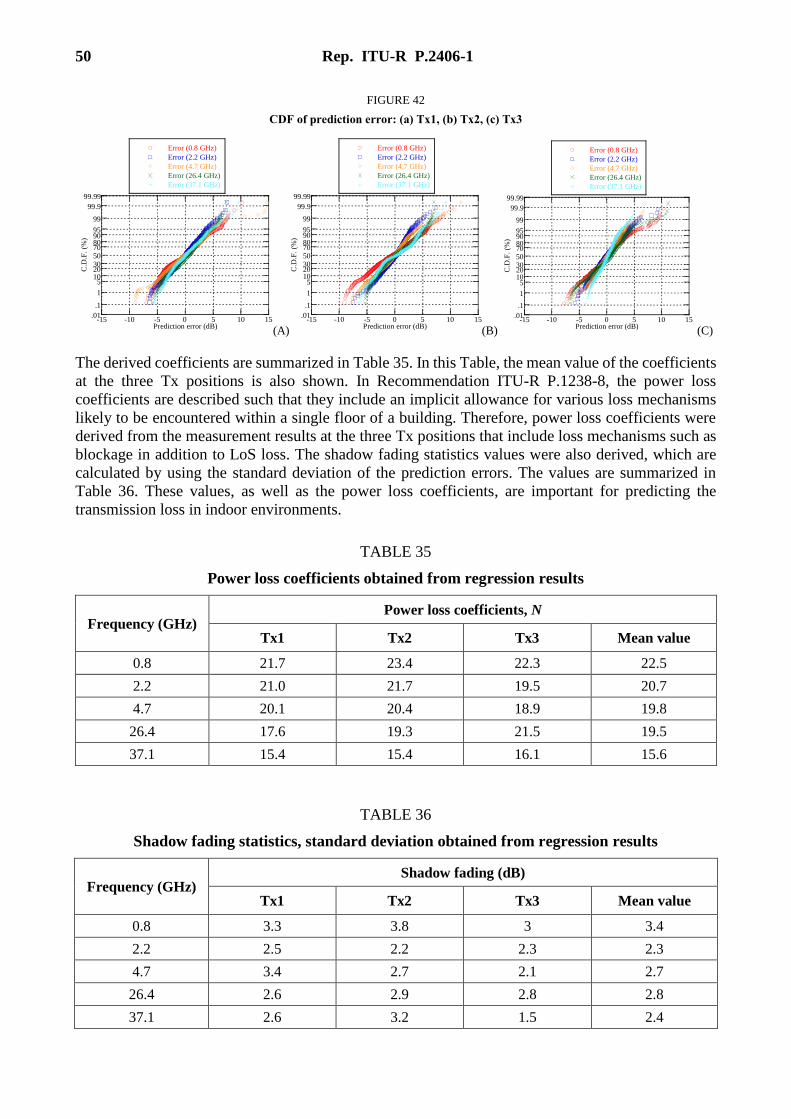
50 Rep. ITU-R P.2406-1
FIGURE 42
CDF of prediction error: (a) Tx1, (b) Tx2, (c) Tx3
(A) (B) (C)
The derived coefficients are summarized in Table 35. In this Table, the mean value of the coefficients
at the three Tx positions is also shown. In Recommendation ITU-R P.1238-8, the power loss
coefficients are described such that they include an implicit allowance for various loss mechanisms
likely to be encountered within a single floor of a building. Therefore, power loss coefficients were
derived from the measurement results at the three Tx positions that include loss mechanisms such as
blockage in addition to LoS loss. The shadow fading statistics values were also derived, which are
calculated by using the standard deviation of the prediction errors. The values are summarized in
Table 36. These values, as well as the power loss coefficients, are important for predicting the
transmission loss in indoor environments.
TABLE 35
Power loss coefficients obtained from regression results
Frequency (GHz) Power loss coefficients, N
Tx1 Tx2 Tx3 Mean value
0.8 21.7 23.4 22.3 22.5
2.2 21.0 21.7 19.5 20.7
4.7 20.1 20.4 18.9 19.8
26.4 17.6 19.3 21.5 19.5
37.1 15.4 15.4 16.1 15.6
TABLE 36
Shadow fading statistics, standard deviation obtained from regression results
Frequency (GHz) Shadow fading (dB)
Tx1 Tx2 Tx3 Mean value
0.8 3.3 3.8 3 3.4
2.2 2.5 2.2 2.3 2.3
4.7 3.4 2.7 2.1 2.7
26.4 2.6 2.9 2.8 2.8
37.1 2.6 3.2 1.5 2.4
-15 -10 -5 0 5 10 15.01
.1
1
51020305070809095
99
99.9
99.99
Error (0.8 GHz)
Error (2.2 GHz)
Error (4.7 GHz)
Error (26.4 GHz)
Error (37.1 GHz)
Prediction error (dB)
C.D
.F.
(%)
-15 -10 -5 0 5 10 15.01
.1
1
51020305070809095
99
99.9
99.99
Error (0.8 GHz)
Error (2.2 GHz)
Error (4.7 GHz)
Error (26.4 GHz)
Error (37.1 GHz)
Prediction error (dB)
C.D
.F.
(%)
-15 -10 -5 0 5 10 15.01
.1
1
51020305070809095
99
99.9
99.99
Error (0.8 GHz)
Error (2.2 GHz)
Error (4.7 GHz)
Error (26.4 GHz)
Error (37.1 GHz)
Prediction error (dB)
C.D
.F.
(%)

Rep. ITU-R P.2406-1 51
In addition, the frequency dependency of the power loss coefficients was analysed. Figure 43 shows
the frequency dependency of (a) the values in Table 35, and (b) the values described in the current
Recommendation ITU-R P.1238. It should be noted that the values in Recommendation ITU-R
P.1238 were derived from measurements in various environments, and so it is difficult to simply
compare with the results obtained here. In this figure, the regressed result is also shown by the solid
line. As can be seen in this figure, the power loss coefficients decrease as the frequency increases,
meaning that they have a frequency dependency. Such frequency dependency could be used for
developing the power loss coefficient model.
FIGURE 43
Frequency dependency of power loss coefficients
(a) Measurement results (b) Values in current Rec. ITU-R P.1238
6.1.5 Summary of the results
This contribution presented measurement results of five frequency bands up to 37 GHz in an office
environment, as well as the power loss coefficients and the shadow fading characteristics. It was
shown that the power loss coefficients have a frequency dependency, which could be used for
developing the power loss coefficient model.
6.2 Study 2: Power loss coefficients and shadow fading statistics
(Frequency bands: 28, 38 GHz)
6.2.1 Executive summary
This section provides additional information for the power loss coefficients and shadow fading
statistics included in Recommendation ITU-R P.1238. This study focuses on the frequency bands
28 GHz and 38 GHz based on measurements made in indoor office and indoor commercial (train
station and airport terminal) environments.
6.2.2 Background and proposal
Table 37 and Table 38 show the proposed power loss coefficients and shadow fading statistics,
respectively.
14
16
18
20
22
24
0.1 1 10 100
Tx1 Tx2 Tx3
Po
wer
lo
ss c
oef
fici
ents
Frequency (GHz)
N = -3.1log(f) + 22.1
15
20
25
30
35
40
45
0.1 1 10 100
ResidentialOffice
CommercialFactory
Corridor
Pow
er l
oss
co
effi
cien
ts
Frequency (GHz)
N = -3.8log(f)+28.3
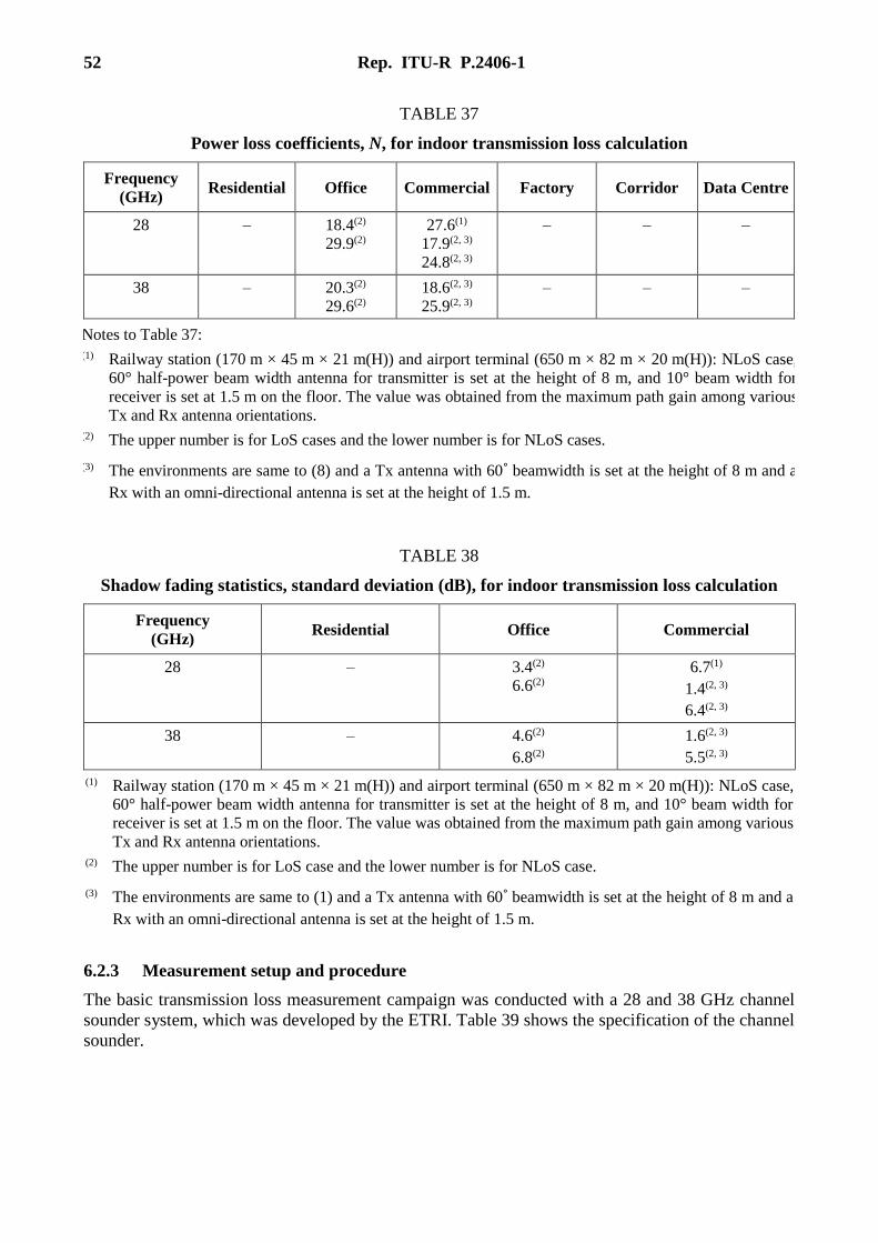
52 Rep. ITU-R P.2406-1
TABLE 37
Power loss coefficients, N, for indoor transmission loss calculation
Frequency
(GHz) Residential Office Commercial Factory Corridor Data Centre
28 – 18.4(2)
29.9(2)
27.6(1)
17.9(2, 3)
24.8(2, 3)
– – –
38 – 20.3(2)
29.6(2)
18.6(2, 3)
25.9(2, 3)
– – –
Notes to Table 37:
(1) Railway station (170 m × 45 m × 21 m(H)) and airport terminal (650 m × 82 m × 20 m(H)): NLoS case,
60° half-power beam width antenna for transmitter is set at the height of 8 m, and 10° beam width for
receiver is set at 1.5 m on the floor. The value was obtained from the maximum path gain among various
Tx and Rx antenna orientations.
(2) The upper number is for LoS cases and the lower number is for NLoS cases.
(3) The environments are same to (8) and a Tx antenna with 60˚ beamwidth is set at the height of 8 m and a
Rx with an omni-directional antenna is set at the height of 1.5 m.
TABLE 38
Shadow fading statistics, standard deviation (dB), for indoor transmission loss calculation
Frequency
(GHz) Residential Office Commercial
28 – 3.4(2)
6.6(2)
6.7(1)
1.4(2, 3)
6.4(2, 3)
38 – 4.6(2)
6.8(2)
1.6(2, 3)
5.5(2, 3)
(1) Railway station (170 m × 45 m × 21 m(H)) and airport terminal (650 m × 82 m × 20 m(H)): NLoS case,
60° half-power beam width antenna for transmitter is set at the height of 8 m, and 10° beam width for
receiver is set at 1.5 m on the floor. The value was obtained from the maximum path gain among various
Tx and Rx antenna orientations.
(2) The upper number is for LoS case and the lower number is for NLoS case.
(3) The environments are same to (1) and a Tx antenna with 60˚ beamwidth is set at the height of 8 m and a
Rx with an omni-directional antenna is set at the height of 1.5 m.
6.2.3 Measurement setup and procedure
The basic transmission loss measurement campaign was conducted with a 28 and 38 GHz channel
sounder system, which was developed by the ETRI. Table 39 shows the specification of the channel
sounder.

Rep. ITU-R P.2406-1 53
TABLE 39
Specification of the channel sounder
Description Specification
Carrier frequency 28 GHz 38 GHz
Channel bandwidth 500 MHz
Maximum TX power 29 dBm 21 dBm
Automatic gain control range < 60 dB
The measurement campaign was conducted in three areas: a) an ETRI office, b) Seoul railway station,
and c) Incheon airport terminal. The ETRI office is a typical indoor office environment. Seoul railway
station and Incheon airport terminal are the representative indoor commercial environments in the
Republic of Korea.
6.2.3.1 Basic transmission loss measurements in indoor office environments
The size of the office is 72 m × 23 m × 2.6 m. There are cubicle areas, meeting rooms, corridors,
pillars, etc. The locations of the TX and RX are shown in Fig. 44. The outside walls are composed of
concrete and large tempered glass, whereas the inside walls and ceilings are made of reinforced
concrete, steel and plaster board. The basic transmission loss measurements were collected at two TX
locations and 48 RX locations. In Fig. 44, the red stars show the TX locations and the blue circles
show the LoS RX locations. The red and green circles show the NLoS RX locations. The heights of
the TX and the RX are 2.5 m and 1.2 m, respectively. The transmitting antenna and the receiving
antenna are omni-directional antennas.
FIGURE 44
Basic transmission loss measurement campaign in an ETRI office (Site 1):
(a) Layout of the measurement scenario, (b) Installation of measurement equipment
(a) (b)
6.2.3.2 Basic transmission loss measurements in indoor commercial environments
The basic transmission loss measurements were collected in two indoor commercial environments.
Horn antennas with 60 and 40 degree beamwidths were used at TX for 28 and 38 GHz measurements,
respectively. The TX antenna direction was fixed to the measurement area. At RX, an omni-
directional antenna was installed. For detail information about the locations of the antennas and the
direction of the transmitting antennas is shown in Figs 45 and 46.
The first measurement site is Seoul railway station as shown in Fig. 45 where the antenna locations
of the measurements are marked. Seoul railway station is a large hall with a dimension of 170 m ×
45 m × 21 m. There are many stores, ticketing boxes, and offices. The ceiling and walls are

54 Rep. ITU-R P.2406-1
constructed with steel frames and thick tempered glasses. In Fig. 45, the blue and green circles denote
LoS locations and NLoS locations, respectively. The TX antenna was set up at 8 m high. The RX
antenna moved while maintaining the antenna height at 1.5 m.
The second site is Incheon airport terminal as shown in Fig. 46. Incheon airport terminal is a very
large hall with a dimension of 650 m × 82 m × 20 m. There are many reception tables, banks, stores,
and many partitions. In Fig. 45, the blue and green circles denote LoS locations and NLoS locations,
respectively. The TX antenna was set up at the height of 8 m. The RX antenna moved at the height
of 1.5 m.
FIGURE 45
Transmission loss measurement campaign in Seoul railway station (Site 2):
(a) Layout of the measurement scenario, (b) Installation of the measurement equipment
(A)
(B) 28GHz Channel Sounder (TX)
RF & Antenna (TX)
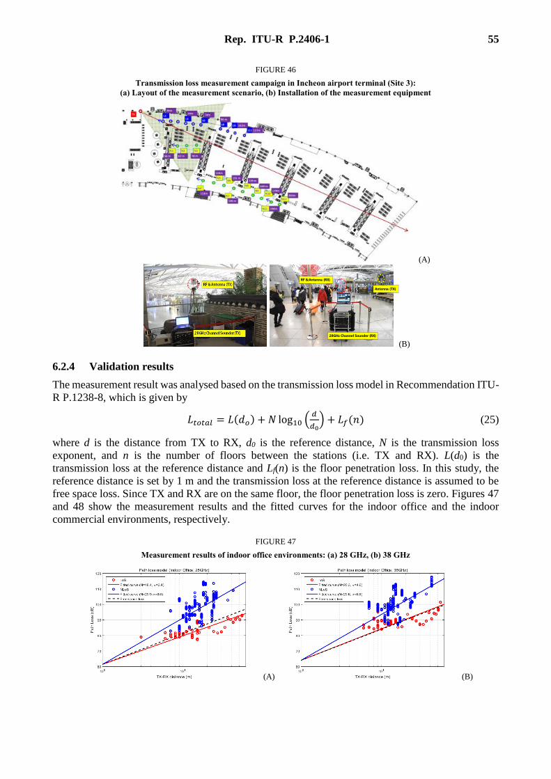
Rep. ITU-R P.2406-1 55
FIGURE 46
Transmission loss measurement campaign in Incheon airport terminal (Site 3):
(a) Layout of the measurement scenario, (b) Installation of the measurement equipment
(A)
(B)
6.2.4 Validation results
The measurement result was analysed based on the transmission loss model in Recommendation ITU-
R P.1238-8, which is given by
𝐿𝑡𝑜𝑡𝑎𝑙 = 𝐿(𝑑𝑜) + 𝑁 log10 (𝑑
𝑑0) + 𝐿𝑓(𝑛) (25)
where d is the distance from TX to RX, d0 is the reference distance, N is the transmission loss
exponent, and n is the number of floors between the stations (i.e. TX and RX). L(d0) is the
transmission loss at the reference distance and Lf(n) is the floor penetration loss. In this study, the
reference distance is set by 1 m and the transmission loss at the reference distance is assumed to be
free space loss. Since TX and RX are on the same floor, the floor penetration loss is zero. Figures 47
and 48 show the measurement results and the fitted curves for the indoor office and the indoor
commercial environments, respectively.
FIGURE 47
Measurement results of indoor office environments: (a) 28 GHz, (b) 38 GHz
(A) (B)
28GHz Channel Sounder (RX)
RF & Antenna (RX)
Antenna (TX)
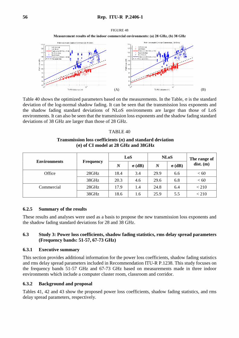
56 Rep. ITU-R P.2406-1
FIGURE 48
Measurement results of the indoor commercial environments: (a) 28 GHz, (b) 38 GHz
(A) (B)
Table 40 shows the optimized parameters based on the measurements. In the Table, σ is the standard
deviation of the log-normal shadow fading. It can be seen that the transmission loss exponents and
the shadow fading standard deviations of NLoS environments are larger than those of LoS
environments. It can also be seen that the transmission loss exponents and the shadow fading standard
deviations of 38 GHz are larger than those of 28 GHz.
TABLE 40
Transmission loss coefficients (n) and standard deviation
(σ) of CI model at 28 GHz and 38GHz
Environments Frequency LoS NLoS The range of
dist. (m) N σ (dB) N σ (dB)
Office 28GHz 18.4 3.4 29.9 6.6 < 60
38GHz 20.3 4.6 29.6 6.8 < 60
Commercial 28GHz 17.9 1.4 24.8 6.4 < 210
38GHz 18.6 1.6 25.9 5.5 < 210
6.2.5 Summary of the results
These results and analyses were used as a basis to propose the new transmission loss exponents and
the shadow fading standard deviations for 28 and 38 GHz.
6.3 Study 3: Power loss coefficients, shadow fading statistics, rms delay spread parameters
(Frequency bands: 51-57, 67-73 GHz)
6.3.1 Executive summary
This section provides additional information for the power loss coefficients, shadow fading statistics
and rms delay spread parameters included in Recommendation ITU-R P.1238. This study focuses on
the frequency bands 51-57 GHz and 67-73 GHz based on measurements made in three indoor
environments which include a computer cluster room, classroom and corridor.
6.3.2 Background and proposal
Tables 41, 42 and 43 show the proposed power loss coefficients, shadow fading statistics, and rms
delay spread parameters, respectively.

Rep. ITU-R P.2406-1 57
TABLE 41
Power loss coefficients, N, for indoor transmission loss calculation
NOTE – The original values from this study were reworked so that they are consistent with the methodology
used for the other values in the corresponding Table in Recommendation ITU-R P.1238. The reworked values
are shown below.
Frequency
(GHz) Residential Office Commercial Factory Corridor Data Centre
51-57 – 15(10) – – 13(10)
16.3(4, 10) –
67-73 – 19(11) – – 16(11)
17.6(4, 11) –
(4) Computer room where there are many computers around the room. (10) Transmit antenna beamwidth 56.3º, synthesised 360º in azimuth at receiver with 19.7º beamwidth in
elevation. (11) Transmit antenna beamwidth 40º, synthesised 360º in azimuth at receiver with 14.4º beamwidth in
elevation.
TABLE 42
Shadow fading statistics, standard deviation (dB), for indoor transmission loss calculation
Frequency
(GHz) Residential Office Commercial
51-57 – 2.7 –
67-73 – 2.1 –
TABLE 43
rms delay spread parameters
Freq.
(GHz)
Environ-
ment
Polari-
zation
Time
delay
resolution
(ns)
Tx beam
width
(degrees)
Rx beam
width
(degrees)
A
(ns)
B
(ns)
C
(ns)
Note
for
A, B, C
51-57
Computer
cluster VV/HH 0.5 56.3
18.4 0.69 0.96 2.89 (1)
18.4(3) 2.14 10.7 29.7 (1, 2)
Office/
classroom VV/HH 0.5 56.3
18.4 0.56 0.65 4.29 (1)
18.4(3) 1.6 15.8 26.7 (1, 2)
Corridor VV/HH 0.5 56.3 18.4 0.54 0.72 1.34 (1)
18.4(3) 0.81 8.9 44.6 (1, 2)
67-73
Computer
cluster VV/HH 0.5 40
14.4 0.36 0.57 2.4 (1)
14.4(3) 1.1 10.9 28.1 (1, 2)
Office/
classroom VV/HH 0.5 40
14.4 0.33 0.5 6.39 (1)
14.4(3) 1.59 12.6 25.9 (1, 2)
Corridor VV/HH 0.5 40 14.4 0.36 0.47 1.2 (1)
14.4(3) 0.49 6.11 35.2 (1, 2)
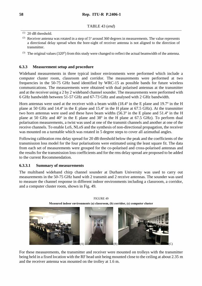
58 Rep. ITU-R P.2406-1
TABLE 43 (end)
(1) 20 dB threshold. (2) Receiver antenna was rotated in a step of 5o around 360 degrees in measurements. The value represents
a directional delay spread when the bore-sight of receiver antenna is not aligned to the direction of
transmitter.
(3) The original values (320º) from this study were changed to reflect the actual beamwidth of the antenna.
6.3.3 Measurement setup and procedure
Wideband measurements in three typical indoor environments were performed which include a
computer cluster room, classroom and corridor. The measurements were performed at two
frequencies in the 50-75 GHz band identified by WRC-15 as possible bands for future wireless
communications. The measurements were obtained with dual polarised antennas at the transmitter
and at the receiver using a 2 by 2 wideband channel sounder. The measurements were performed with
6 GHz bandwidth between 51-57 GHz and 67-73 GHz and analysed with 2 GHz bandwidth.
Horn antennas were used at the receiver with a beam width (18.4º in the E plane and 19.7º in the H
plane at 50 GHz and 14.4º in the E plane and 15.4º in the H plane at 67.5 GHz). At the transmitter
two horn antennas were used and these have beam widths (56.3º in the E plane and 51.4º in the H
plane at 50 GHz and 40º in the E plane and 38º in the H plane at 67.5 GHz). To perform dual
polarisation measurements, a twist was used at one of the transmit channels and another at one of the
receive channels. To enable LoS, NLoS and the synthesis of non-directional propagation, the receiver
was mounted on a turntable which was rotated in 5 degree steps to cover all azimuthal angles.
Following calibration rms delay spread for 20 dB threshold below the peak and the coefficients of the
transmission loss model for the four polarisations were estimated using the least square fit. The data
from each set of measurements were grouped for the co-polarised and cross-polarised antennas and
the results for the transmission loss coefficients and for the rms delay spread are proposed to be added
to the current Recommendation.
6.3.3.1 Summary of measurements
The multiband wideband chirp channel sounder at Durham University was used to carry out
measurements in the 50-75 GHz band with 2 transmit and 2 receive antennas. The sounder was used
to measure the channel response in different indoor environments including a classroom, a corridor,
and a computer cluster room, shown in Fig. 49.
FIGURE 49
Measured indoor environments (a) classroom, (b) corridor, (c) computer cluster
(A) (B) (C)
For these measurements, the transmitter and receiver were mounted on trolleys with the transmitter
being held in a fixed location with the RF head unit being mounted close to the ceiling at about 2.35 m
and the receiver antenna was mounted on the trolley at 1.6 m.
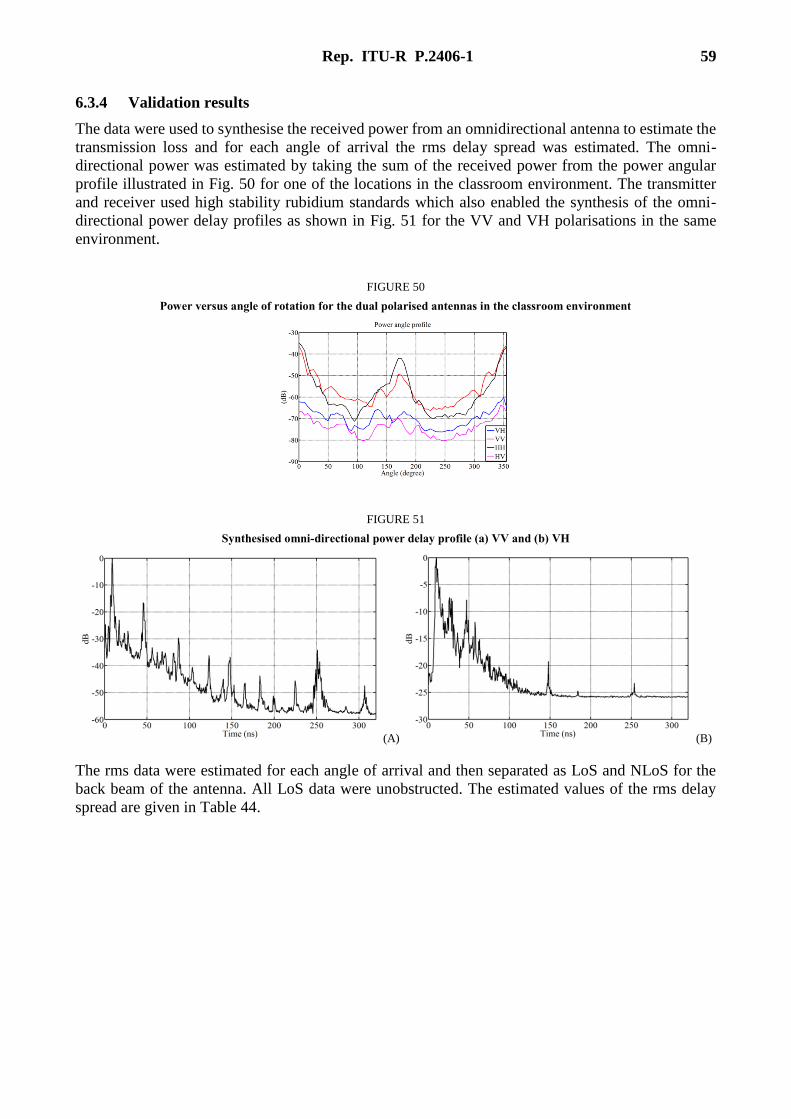
Rep. ITU-R P.2406-1 59
6.3.4 Validation results
The data were used to synthesise the received power from an omnidirectional antenna to estimate the
transmission loss and for each angle of arrival the rms delay spread was estimated. The omni-
directional power was estimated by taking the sum of the received power from the power angular
profile illustrated in Fig. 50 for one of the locations in the classroom environment. The transmitter
and receiver used high stability rubidium standards which also enabled the synthesis of the omni-
directional power delay profiles as shown in Fig. 51 for the VV and VH polarisations in the same
environment.
FIGURE 50
Power versus angle of rotation for the dual polarised antennas in the classroom environment
FIGURE 51
Synthesised omni-directional power delay profile (a) VV and (b) VH
(A) (B)
The rms data were estimated for each angle of arrival and then separated as LoS and NLoS for the
back beam of the antenna. All LoS data were unobstructed. The estimated values of the rms delay
spread are given in Table 44.
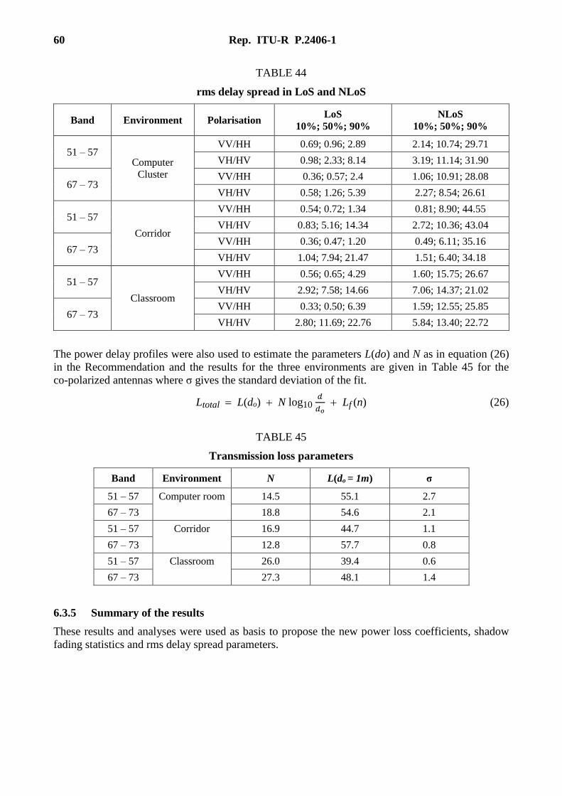
60 Rep. ITU-R P.2406-1
TABLE 44
rms delay spread in LoS and NLoS
Band Environment Polarisation LoS
10%; 50%; 90%
NLoS
10%; 50%; 90%
51 – 57 Computer
Cluster
VV/HH 0.69; 0.96; 2.89 2.14; 10.74; 29.71
VH/HV 0.98; 2.33; 8.14 3.19; 11.14; 31.90
67 – 73 VV/HH 0.36; 0.57; 2.4 1.06; 10.91; 28.08
VH/HV 0.58; 1.26; 5.39 2.27; 8.54; 26.61
51 – 57
Corridor
VV/HH 0.54; 0.72; 1.34 0.81; 8.90; 44.55
VH/HV 0.83; 5.16; 14.34 2.72; 10.36; 43.04
67 – 73 VV/HH 0.36; 0.47; 1.20 0.49; 6.11; 35.16
VH/HV 1.04; 7.94; 21.47 1.51; 6.40; 34.18
51 – 57
Classroom
VV/HH 0.56; 0.65; 4.29 1.60; 15.75; 26.67
VH/HV 2.92; 7.58; 14.66 7.06; 14.37; 21.02
67 – 73 VV/HH 0.33; 0.50; 6.39 1.59; 12.55; 25.85
VH/HV 2.80; 11.69; 22.76 5.84; 13.40; 22.72
The power delay profiles were also used to estimate the parameters L(do) and N as in equation (26)
in the Recommendation and the results for the three environments are given in Table 45 for the
co-polarized antennas where σ gives the standard deviation of the fit.
Ltotal L(do) N log10 𝑑
𝑑𝑜 Lf (n) (26)
TABLE 45
Transmission loss parameters
Band Environment N L(do = 1m) σ
51 – 57 Computer room 14.5 55.1 2.7
67 – 73 18.8 54.6 2.1
51 – 57 Corridor 16.9 44.7 1.1
67 – 73 12.8 57.7 0.8
51 – 57 Classroom 26.0 39.4 0.6
67 – 73 27.3 48.1 1.4
6.3.5 Summary of the results
These results and analyses were used as basis to propose the new power loss coefficients, shadow
fading statistics and rms delay spread parameters.

Rep. ITU-R P.2406-1 61
6.4 Study 4: Power loss coefficients (Frequency band: 70 GHz)
6.4.1 Executive summary
This section provides additional information for the power loss coefficients included in
Recommendation ITU-R P.1238. This study focuses on the frequency band 70 GHz based on
measurements made in an indoor office environment.
6.4.2 Background and proposal
Table 46 shows the proposed power loss coefficient.
TABLE 46
Power loss coefficients, N, for indoor transmission loss calculation
Frequency
(GHz) Residential Office Commercial Factory Corridor Data Centre
70 – 22(1) – – – –
(1) 60 GHz and 70 GHz values assume propagation within a single room or space, and do not include any
allowance for transmission through walls. Gaseous absorption around 60 GHz is also significant for
distances greater than about 100 m which may influence frequency reuse distances (see Recommendation
ITU-R P.676).
6.4.3 Measurement setup and procedure
Measurements were performed in an office. The area measured was 22 × 12.5 × 3.5 m. The walls
were made of metal, and metal bookshelves were set along the walls. Along the window, there were
low bookshelves also made of metal. The ceiling was made of plasterboard, and fluorescent lights
and air conditioning units were positioned on the ceiling. The flooring was made of metal, which was
covered by a carpet. Table 47 shows the measurement parameters, and Fig. 52 shows the measurement
conditions in the office.
TABLE 47
Measurement conditions (Office)
Frequency Polarization Tx antenna Rx antenna Environment Antenna
height
70 GHz V 60° 15°, 30°, 60° LoS 1, 2, 3, 5, 7, 10, 14 m 1 m
70 GHz V 60° 15°, 30°, 60° NLoS 3, 7, 10, 14 m 1 m

62 Rep. ITU-R P.2406-1
FIGURE 52
Measurement environment (Office)
We measured the distance characteristics on the passage and desk sides of the office. The LoS was
between the Tx and Rx on the passage side. Because the average height of the office fixtures on the
desk side was 1.2 m, the environment between the Tx and Rx could be classified as a NLoS.
6.4.4 Validation results
Figure 53 shows the measurement results. N was obtained by using the least square method for each
environment. Equation (1) with N=20 and 24 approximates the LOS and NLOS in the office results
well, respectively. N=22 approximates the total results. The results are summarized in Table 48.
FIGURE 53
Measurement results
TABLE 48
Power loss coefficients N
Frequency Office (LoS) Office (NLoS) Office (Total)
70 GHz* 20 24 22
* 70 GHz values assume propagation within a single room or space, and do not include any allowance for
transmission through walls.
6.4.5 Results of studies
Based on the results and analyses above, a new power loss coefficient value is proposed for 70 GHz.

Rep. ITU-R P.2406-1 63
6.5 Study 5: Power loss coefficients
6.5.1 Executive summary
This section provides additional information for the power loss coefficients included in
Recommendation ITU-R P.1238. This study focuses on the frequency band 300 GHz based on
measurements made in indoor office and corridor environments.
6.5.2 Background and proposal
Table 49 shows the proposed power loss coefficients.
TABLE 49
Power loss coefficients, N, for indoor transmission loss calculation
Frequency
(GHz) Residential Office Commercial Factory Corridor Data Centre
300 – 20(15) – – 19.5(9, 15) 20.2(15)
(9) Transmitter and receiver are on LoS corridor. (15) Transmit and received antennas have 10° beamwidth.
6.5.3 Measurement setup and procedure
6.5.3.1 First measurement campaign – office and corridor environments
In a first measurement campaign, propagation loss was measured by using 300 GHz continuous wave
in an anechoic chamber as shown in Fig. 54 to confirm the transmitter (TX) and receiver (RX).
Subsequently propagation loss in office and corridor environments was measured. The maximum
transmission distance was a few tens of meters in the line-of-sight situation because the output power
was limited to ‒15 dBm by a used RF device performance. In the measurement, directional antennas
were used by considering actual 300 GHz wireless applications. The aperture size of antenna is
6 mm × 8.36 mm and the antenna gain is 25 dBi as shown in Fig. 55. The antenna heights of TX and
RX were 1.1 m above the floor. The measured polarization was set to vertical. For transmission loss
measurement, the TX was fixed and RX was moved by using a platform truck. Table 50 summarizes
these parameters.
FIGURE 54
Propagation measurement in anechoic chamber
Signal generator
External mixer
Spectrum analyser
Signal generator
Source module

64 Rep. ITU-R P.2406-1
FIGURE 55
Standard gain horn antenna
(a) Standard gain horn (b) Simulated antenna directivity
TABLE 50
Measurement parameters
Measured frequency 300 GHz (CW)
Output power −15 dBm
TX and RX antennas
Standard gain horn
Gain: 25 dBi (HPBW 10 degree)
Height: 1.1 m above the floor
Figure 56 shows the measurement system for indoor environments. The TX and RX were put on the
trucks and the RX position was changed in the measurement. There was no human in the
environments during the measurement to keep the static condition. The measured distance was up to
12 m for office and 35 m for corridor environments in the line-of-sight situation.
FIGURE 56
Measurement system for indoor environment.
The snapshots of transmitter and receiver are shown in Fig. 57. The indoor measurement was carried
out in the office and corridor environments as shown in Fig. 58.
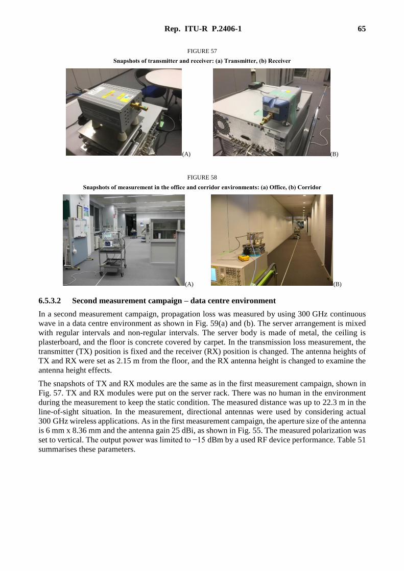
Rep. ITU-R P.2406-1 65
FIGURE 57
Snapshots of transmitter and receiver: (a) Transmitter, (b) Receiver
(A) (B)
FIGURE 58
Snapshots of measurement in the office and corridor environments: (a) Office, (b) Corridor
(A) (B)
6.5.3.2 Second measurement campaign – data centre environment
In a second measurement campaign, propagation loss was measured by using 300 GHz continuous
wave in a data centre environment as shown in Fig. 59(a) and (b). The server arrangement is mixed
with regular intervals and non-regular intervals. The server body is made of metal, the ceiling is
plasterboard, and the floor is concrete covered by carpet. In the transmission loss measurement, the
transmitter (TX) position is fixed and the receiver (RX) position is changed. The antenna heights of
TX and RX were set as 2.15 m from the floor, and the RX antenna height is changed to examine the
antenna height effects.
The snapshots of TX and RX modules are the same as in the first measurement campaign, shown in
Fig. 57. TX and RX modules were put on the server rack. There was no human in the environment
during the measurement to keep the static condition. The measured distance was up to 22.3 m in the
line-of-sight situation. In the measurement, directional antennas were used by considering actual
300 GHz wireless applications. As in the first measurement campaign, the aperture size of the antenna
is 6 mm x 8.36 mm and the antenna gain 25 dBi, as shown in Fig. 55. The measured polarization was
set to vertical. The output power was limited to −15 dBm by a used RF device performance. Table 51
summarises these parameters.

66 Rep. ITU-R P.2406-1
FIGURE 59
(a) Data centre environment, (b) Server arrangement in the data centre
(A) (B)
TABLE 51
Measurement parameters – second measurement campaign
Measured frequency 300 GHz (CW)
Output power −15 dBm
TX and RX antennas Rectangular horn
Gain: 25 dBi (HPBW 10 degree)
6.5.4 Validation results
6.5.4.1 Results for the office and corridor environments
The relationship between the received power and the transmission distance in the anechoic chamber
is shown in Fig. 60. In this Figure the simulation result by a moment method (MoM) including
antenna structure is also plotted. It was confirmed that the pass loss coefficient is N = 20 identical
with the free space loss in the far field.
FIGURE 60
Received power measurement in the anechoic chamber
Measured transmission loss results in the office and corridor environments are shown in Fig. 61. By
a linear approximations, transmission loss coefficients were extracted as N = 20 and 19.5 for each
environment. The coefficient of office environment was roughly identical with the free space loss,
because antenna half power beam width was narrow as 10 degrees. The coefficient of corridor
environment was slightly decreased from N = 20.

Rep. ITU-R P.2406-1 67
FIGURE 61
Measured transmission loss results (a) in the office environment, (b) in the corridor environment
(A) (B)

68 Rep. ITU-R P.2406-1
6.5.4.2 Results for the data centre environment
The relationship between the measured transmission loss and the transmission distance in the data
centre is shown in Fig. 62. By a linear approximation, transmission loss coefficients were extracted
as N = 20.2. The coefficient of the data centre environment was roughly identical with the free space
loss, however, it had about ±5 dB deviation.
FIGURE 62
Measured transmission loss results in the data centre environment
6.5.5 Summary of the results
The transmission loss coefficients of office and corridor environments at 300 GHz have been
extracted using directional antennas. The coefficient of office environment was roughly identical with
the free space loss of N = 20, and the coefficient of corridor environment was slightly decreased to N
= 19.5. These parameters are also close in value to the coefficient at 60 and 70 GHz of
Recommendation ITU-R P.1238.
The transmission loss coefficients of a data centre environment at 300 GHz have been extracted using
directional antennas. The transmission loss coefficient was N = 20.2 which is roughly identical with
the free space loss of N = 20, however, it has a ±5 dB deviation by interference of direct and reflection
waves.
The new power loss coefficients were proposed based on the results and analyses.
6.6 Study 6: Rms delay spread parameters (Frequency bands: 28, 38 GHz)
6.6.1 Executive summary
This study provides additional information for the rms delay spread parameters included in
Recommendation ITU-R P.1238. This study focuses on the frequency bands 28 and 38 GHz based
on measurements made in indoor commercial environments (Seoul railway station and Incheon
international airport terminal)
6.6.2 Background and proposal
Table 52 shows the proposed rms delay spread parameters.

Rep. ITU-R P.2406-1 69
TABLE 52
rms delay spread parameters
Freq.
(GHz)
Environ-
ment
Polari-
zation
Time
delay
resolution
(ns)
Tx beam
width
(degrees)
Rx beam
width
(degrees)
A
(ns)
B
(ns)
C
(ns)
Note
for
A, B, C
28 Commercial VV 2 60 Omni 17
36
34
65
64
86 (1, 2)
38 Commercial VV 2 40 Omni 4
42
26
69
55
82 (1, 2)
(1) Upper and lower values are LoS and NLoS cases, respectively.
(2) 20 dB threshold.
6.6.3 Measurement setup and procedure
6.6.3.1 Channel sounder
The channel sounder operates with 4 095 chips pseudo random noise (PN) mode, 500 Mcps chip
rates, 2 ns measurement resolution. A channel sounder was implemented using a swept time delay
cross-correlation technique. Transmitter (TX) is installed at the height (Hb) of 8.2 m. Its conducting
power is 29 dBm at 28 GHz and 21 dBm at 38 GHz carrier frequency. A receiver is at the height
(Hm) of 1.7 m. During the measurement, the location of a TX was fixed, and a RX on the floor was
positioned at LoS or NLoS environments. A TX antenna has the directional horn type with half-
power-beamwidth (HPBW) of 40⁰ at 38 GHz or 60⁰ at 28 GHz in order to mostly cover the
measurement area (railway station or airport terminal), and a RX antenna has the beam pattern of
omnidirectional type. Both the TX and RX antenna have the same vertically polarization.
6.6.3.2 Omnidirectional measurements in an indoor commercial environment
Measurements were performed in the Seoul railway station and the Incheon airport terminal in the
Republic of Korea. The features of these indoor environments are given below and shown in Fig. 63.
– Site 1 (Seoul railway station): The measurement was carried out in a large hall with a
dimension of 80 m (length) 45 m (width) 21 m (height) located on the 1st floor of terminal
building. The ceiling and walls of the hall are built with steel frames and thick tempered
glasses. The floors are constructed with steel-reinforced concrete. There are offices, ticketing
boxes and shops in the hall. A large electric notice board informing train departure-and-
arrival time is on the wall.
– Site 2 (Incheon airport terminal): The measurement has been carried out in a big hall with a
dimension of 320 m (length) 82 m (width) 20 m (height) which is on the third floor of
the airport passenger terminal building. Building materials are similar to the Seoul railway
station except for parallel arranged check-in booths.
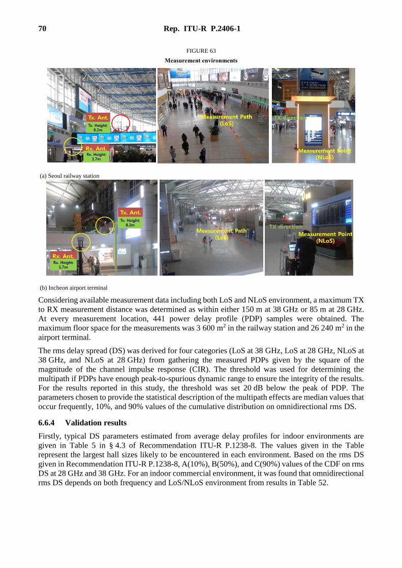
70 Rep. ITU-R P.2406-1
FIGURE 63
Measurement environments
(a) Seoul railway station
(b) Incheon airport terminal
Considering available measurement data including both LoS and NLoS environment, a maximum TX
to RX measurement distance was determined as within either 150 m at 38 GHz or 85 m at 28 GHz.
At every measurement location, 441 power delay profile (PDP) samples were obtained. The
maximum floor space for the measurements was 3 600 m2 in the railway station and 26 240 m2 in the
airport terminal.
The rms delay spread (DS) was derived for four categories (LoS at 38 GHz, LoS at 28 GHz, NLoS at
38 GHz, and NLoS at 28 GHz) from gathering the measured PDPs given by the square of the
magnitude of the channel impulse response (CIR). The threshold was used for determining the
multipath if PDPs have enough peak-to-spurious dynamic range to ensure the integrity of the results.
For the results reported in this study, the threshold was set 20 dB below the peak of PDP. The
parameters chosen to provide the statistical description of the multipath effects are median values that
occur frequently, 10%, and 90% values of the cumulative distribution on omnidirectional rms DS.
6.6.4 Validation results
Firstly, typical DS parameters estimated from average delay profiles for indoor environments are
given in Table 5 in § 4.3 of Recommendation ITU-R P.1238-8. The values given in the Table
represent the largest hall sizes likely to be encountered in each environment. Based on the rms DS
given in Recommendation ITU-R P.1238-8, A(10%), B(50%), and C(90%) values of the CDF on rms
DS at 28 GHz and 38 GHz. For an indoor commercial environment, it was found that omnidirectional
rms DS depends on both frequency and LoS/NLoS environment from results in Table 52.

Rep. ITU-R P.2406-1 71
6.6.5 Summary of the results
This study describes additional information on measurement environment and the process for
deriving the proposed rms delay spread parameters. From the results, these parameters could be
applied for indoor environments such as public commercial indoor area at 28 and 38 GHz.
6.7 Study 7: Rms delay spread parameters (Frequency bands: 30, 60 GHz)
6.7.1 Executive summary
This study provides additional information for the rms delay spread parameters included in
Recommendation ITU-R P.1238. This study focuses on the frequency band 60 GHz based on
measurements made in various indoor office environments (computer cluster, office/classroom,
corridor).
6.7.2 Background and proposal
Table 53 shows the proposed rms delay spread parameters.
TABLE 53
rms delay spread parameters
Freq.
(GHz)
Environ-
ment
Polari-
zation
Time
delay
resolution
(ns)
Tx beam
width
(degrees)
Rx beam
width
(degrees)
A
(ns)
B
(ns)
C
(ns)
Note
for
A, B, C
29.3-
31.5
Computer
cluster Dual(1)
0.45 35 35 1.2 2.5 14 (2)
0.45 35 35 1.6 17.6 34 (3)
18.4 2.14 10.7 29.7 (2, 8)
Office/
classroom VV/HH 0.5 56.3
18.4 0.56 0.65 4.29 (2)
18.4 1.6 15.8 26.7 (2, 8)
Corridor VV/HH 0.5 56.3 18.4 0.54 0.72 1.34 (2)
18.4 0.81 8.9 44.6 (2, 8)
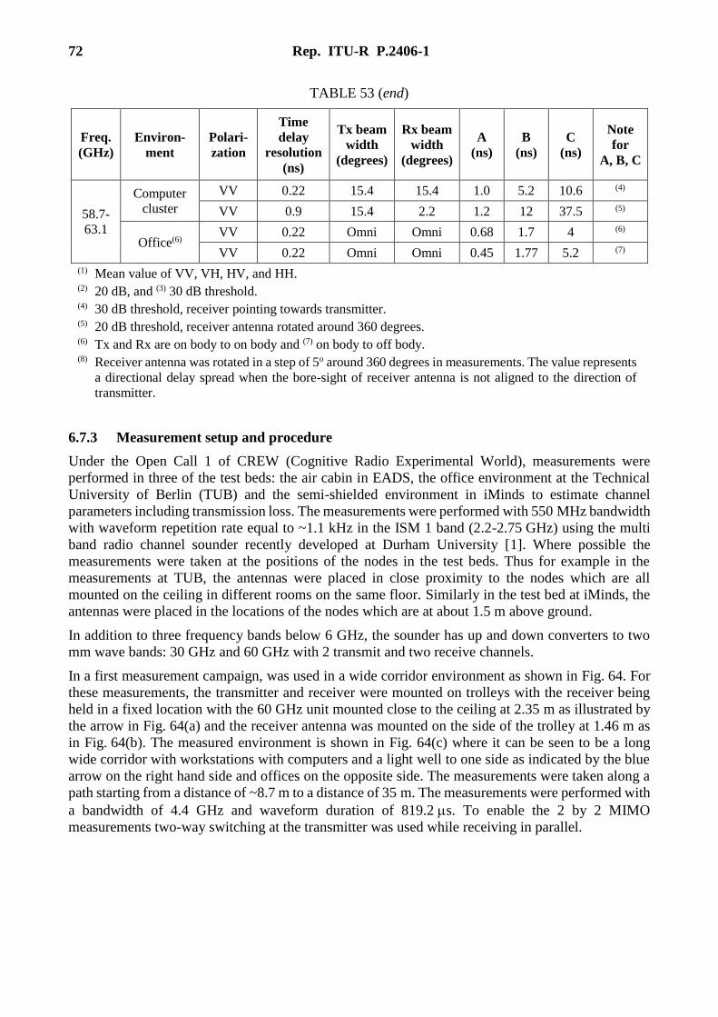
72 Rep. ITU-R P.2406-1
TABLE 53 (end)
Freq.
(GHz)
Environ-
ment
Polari-
zation
Time
delay
resolution
(ns)
Tx beam
width
(degrees)
Rx beam
width
(degrees)
A
(ns)
B
(ns)
C
(ns)
Note
for
A, B, C
58.7-
63.1
Computer
cluster
VV 0.22 15.4 15.4 1.0 5.2 10.6 (4)
VV 0.9 15.4 2.2 1.2 12 37.5 (5)
Office(6) VV 0.22 Omni Omni 0.68 1.7 4 (6)
VV 0.22 Omni Omni 0.45 1.77 5.2 (7)
(1) Mean value of VV, VH, HV, and HH.
(2) 20 dB, and (3) 30 dB threshold. (4) 30 dB threshold, receiver pointing towards transmitter. (5) 20 dB threshold, receiver antenna rotated around 360 degrees. (6) Tx and Rx are on body to on body and (7) on body to off body. (8) Receiver antenna was rotated in a step of 5o around 360 degrees in measurements. The value represents
a directional delay spread when the bore-sight of receiver antenna is not aligned to the direction of
transmitter.
6.7.3 Measurement setup and procedure
Under the Open Call 1 of CREW (Cognitive Radio Experimental World), measurements were
performed in three of the test beds: the air cabin in EADS, the office environment at the Technical
University of Berlin (TUB) and the semi-shielded environment in iMinds to estimate channel
parameters including transmission loss. The measurements were performed with 550 MHz bandwidth
with waveform repetition rate equal to ~1.1 kHz in the ISM 1 band (2.2-2.75 GHz) using the multi
band radio channel sounder recently developed at Durham University [1]. Where possible the
measurements were taken at the positions of the nodes in the test beds. Thus for example in the
measurements at TUB, the antennas were placed in close proximity to the nodes which are all
mounted on the ceiling in different rooms on the same floor. Similarly in the test bed at iMinds, the
antennas were placed in the locations of the nodes which are at about 1.5 m above ground.
In addition to three frequency bands below 6 GHz, the sounder has up and down converters to two
mm wave bands: 30 GHz and 60 GHz with 2 transmit and two receive channels.
In a first measurement campaign, was used in a wide corridor environment as shown in Fig. 64. For
these measurements, the transmitter and receiver were mounted on trolleys with the receiver being
held in a fixed location with the 60 GHz unit mounted close to the ceiling at 2.35 m as illustrated by
the arrow in Fig. 64(a) and the receiver antenna was mounted on the side of the trolley at 1.46 m as
in Fig. 64(b). The measured environment is shown in Fig. 64(c) where it can be seen to be a long
wide corridor with workstations with computers and a light well to one side as indicated by the blue
arrow on the right hand side and offices on the opposite side. The measurements were taken along a
path starting from a distance of ~8.7 m to a distance of 35 m. The measurements were performed with
a bandwidth of 4.4 GHz and waveform duration of 819.2 s. To enable the 2 by 2 MIMO
measurements two-way switching at the transmitter was used while receiving in parallel.
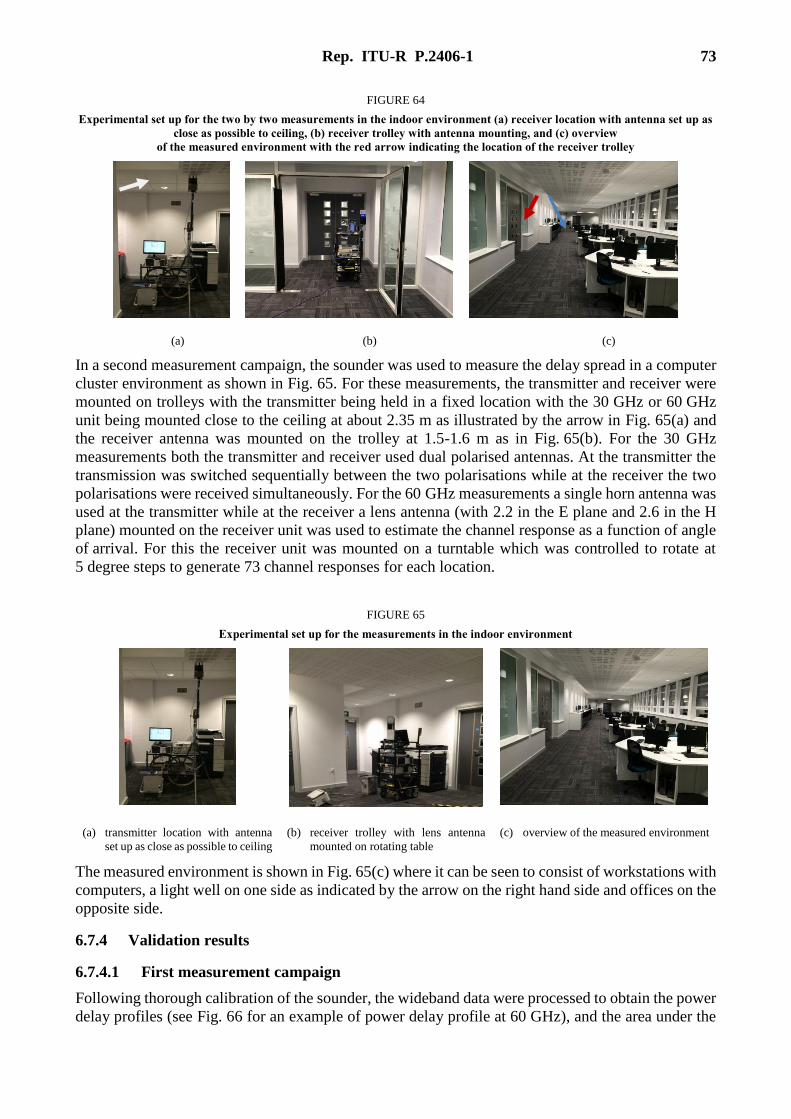
Rep. ITU-R P.2406-1 73
FIGURE 64
Experimental set up for the two by two measurements in the indoor environment (a) receiver location with antenna set up as
close as possible to ceiling, (b) receiver trolley with antenna mounting, and (c) overview
of the measured environment with the red arrow indicating the location of the receiver trolley
(a) (b) (c)
In a second measurement campaign, the sounder was used to measure the delay spread in a computer
cluster environment as shown in Fig. 65. For these measurements, the transmitter and receiver were
mounted on trolleys with the transmitter being held in a fixed location with the 30 GHz or 60 GHz
unit being mounted close to the ceiling at about 2.35 m as illustrated by the arrow in Fig. 65(a) and
the receiver antenna was mounted on the trolley at 1.5-1.6 m as in Fig. 65(b). For the 30 GHz
measurements both the transmitter and receiver used dual polarised antennas. At the transmitter the
transmission was switched sequentially between the two polarisations while at the receiver the two
polarisations were received simultaneously. For the 60 GHz measurements a single horn antenna was
used at the transmitter while at the receiver a lens antenna (with 2.2 in the E plane and 2.6 in the H
plane) mounted on the receiver unit was used to estimate the channel response as a function of angle
of arrival. For this the receiver unit was mounted on a turntable which was controlled to rotate at
5 degree steps to generate 73 channel responses for each location.
FIGURE 65
Experimental set up for the measurements in the indoor environment
(a) transmitter location with antenna
set up as close as possible to ceiling
(b) receiver trolley with lens antenna
mounted on rotating table
(c) overview of the measured environment
The measured environment is shown in Fig. 65(c) where it can be seen to consist of workstations with
computers, a light well on one side as indicated by the arrow on the right hand side and offices on the
opposite side.
6.7.4 Validation results
6.7.4.1 First measurement campaign
Following thorough calibration of the sounder, the wideband data were processed to obtain the power
delay profiles (see Fig. 66 for an example of power delay profile at 60 GHz), and the area under the

74 Rep. ITU-R P.2406-1
profile integrated to estimate the received energy as in equation (1) of Recommendation ITU-R
P.1407.
FIGURE 66
Power delay profile at 60 GHz for a single channel in one of the measured locations
The transmission loss was then evaluated where in the TUB and iMinds measurements wideband
omni-directional antennas were used and in the 60 GHz measurements, two horn antennas with
directional beam equal to 15.4o.
The estimated transmission loss dependence on distance in the 2.625 GHz band in the two measured
environments is shown in Fig. 67(a) and (b) where the slope of the curve, n is equal to 4.4 for the
office environment in the TUB data and 3.3 for the iMinds measurements.
FIGURE 67
Estimated transmission loss in (a) office environment in TUB and (b) iMinds with
the transmission loss coefficient fit
(a) (b)
Since all the measurements displayed a dynamic range of at least 40 dB the rms delay spread was
computed for 20 and 30 dB threshold levels. The resulting CDF for the thresholds is shown in Fig. 68
which also displays the rms delay spread for the 30 dB threshold for all the four MIMO channels.
The Figure shows that the difference between the four MIMO channels is small. Taking the median
values gives an rms delay spread of 0.42, and 5.13 ns for the 20, and 30 dB thresholds, respectively
and corresponding 90% values equal to 0.69, and 10.65 ns. The 20 dB threshold is seen in the main
to capture the dominant components whereas the lower threshold captures the farther away
components.
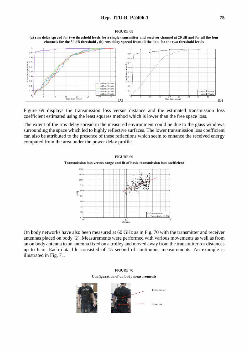
Rep. ITU-R P.2406-1 75
FIGURE 68
(a) rms delay spread for two threshold levels for a single transmitter and receiver channel at 20 dB and for all the four
channels for the 30 dB threshold , (b) rms delay spread from all the data for the two threshold levels
(A) (B)
Figure 69 displays the transmission loss versus distance and the estimated transmission loss
coefficient estimated using the least squares method which is lower than the free space loss.
The extent of the rms delay spread in the measured environment could be due to the glass windows
surrounding the space which led to highly reflective surfaces. The lower transmission loss coefficient
can also be attributed to the presence of these reflections which seem to enhance the received energy
computed from the area under the power delay profile.
FIGURE 69
Transmission loss versus range and fit of basic transmission loss coefficient
On body networks have also been measured at 60 GHz as in Fig. 70 with the transmitter and receiver
antennas placed on body [2]. Measurements were performed with various movements as well as from
an on body antenna to an antenna fixed on a trolley and moved away from the transmitter for distances
up to 6 m. Each data file consisted of 15 second of continuous measurements. An example is
illustrated in Fig. 71.
FIGURE 70
Configuration of on body measurements
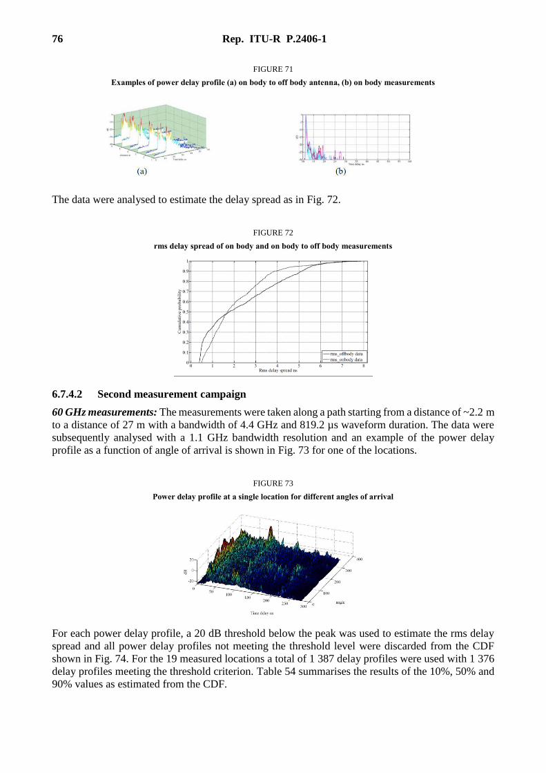
76 Rep. ITU-R P.2406-1
FIGURE 71
Examples of power delay profile (a) on body to off body antenna, (b) on body measurements
The data were analysed to estimate the delay spread as in Fig. 72.
FIGURE 72
rms delay spread of on body and on body to off body measurements
6.7.4.2 Second measurement campaign
60 GHz measurements: The measurements were taken along a path starting from a distance of ~2.2 m
to a distance of 27 m with a bandwidth of 4.4 GHz and 819.2 µs waveform duration. The data were
subsequently analysed with a 1.1 GHz bandwidth resolution and an example of the power delay
profile as a function of angle of arrival is shown in Fig. 73 for one of the locations.
FIGURE 73
Power delay profile at a single location for different angles of arrival
For each power delay profile, a 20 dB threshold below the peak was used to estimate the rms delay
spread and all power delay profiles not meeting the threshold level were discarded from the CDF
shown in Fig. 74. For the 19 measured locations a total of 1 387 delay profiles were used with 1 376
delay profiles meeting the threshold criterion. Table 54 summarises the results of the 10%, 50% and
90% values as estimated from the CDF.

Rep. ITU-R P.2406-1 77
FIGURE 74
Cumulative distribution function of rms delay spread for lens antenna for all angles of arrival
TABLE 54
Summary of rms delay spread for 20 dB threshold for different antenna orientation
Parameter 10% 50% 90%
20 dB rms delay spread 1.2 ns 12 ns 37.5 ns
30 GHz measurements: The measurements were performed with 2.2 GHz bandwidth and 819.2 s
waveform duration. A total of 21 locations were measured over distances from 3 to 31 m. The transmit
antenna mounted at 2.25 m and the receiver antenna at 1.3 m above ground. Dual polarised antennas
at both ends were used. Figure 75 displays the normalised power delay profile for the four channels
whereas Fig. 76 displays the relative power delay profiles for the 21 locations for the V to H polarised
antennas.
FIGURE 75
Power delay profiles with the dual polarised antennas (top left) V to H, (top right) V to V,
(bottom left) H to H, (bottom right) H to V
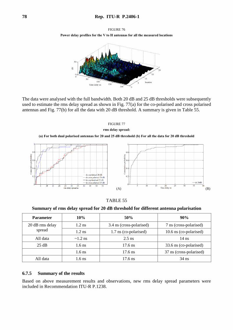
78 Rep. ITU-R P.2406-1
FIGURE 76
Power delay profiles for the V to H antennas for all the measured locations
The data were analysed with the full bandwidth. Both 20 dB and 25 dB thresholds were subsequently
used to estimate the rms delay spread as shown in Fig. 77(a) for the co-polarised and cross polarised
antennas and Fig. 77(b) for all the data with 20 dB threshold. A summary is given in Table 55.
FIGURE 77
rms delay spread:
(a) For both dual polarised antennas for 20 and 25 dB threshold (b) For all the data for 20 dB threshold
(A) (B)
TABLE 55
Summary of rms delay spread for 20 dB threshold for different antenna polarisation
Parameter 10% 50% 90%
20 dB rms delay
spread
1.2 ns 3.4 ns (cross-polarised) 7 ns (cross-polarised)
1.2 ns 1.7 ns (co-polarised) 10.6 ns (co-polarised)
All data ~1.2 ns 2.5 ns 14 ns
25 dB 1.6 ns 17.6 ns 33.6 ns (co-polarised)
1.6 ns 17.6 ns 37 ns (cross-polarised)
All data 1.6 ns 17.6 ns 34 ns
6.7.5 Summary of the results
Based on above measurement results and observations, new rms delay spread parameters were
included in Recommendation ITU-R P.1238.
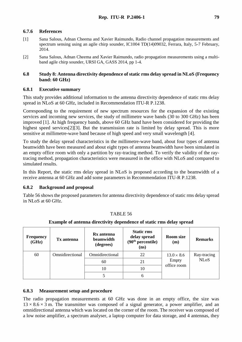
Rep. ITU-R P.2406-1 79
6.7.6 References
[1] Sana Salous, Adnan Cheema and Xavier Raimundo, Radio channel propagation measurements and
spectrum sensing using an agile chirp sounder, IC1004 TD(14)09032, Ferrara, Italy, 5-7 February,
2014.
[2] Sana Salous, Adnan Cheema and Xavier Raimundo, radio propagation measurements using a multi-
band agile chirp sounder, URSI GA, GASS 2014, pp 1-4.
6.8 Study 8: Antenna directivity dependence of static rms delay spread in NLoS (Frequency
band: 60 GHz)
6.8.1 Executive summary
This study provides additional information to the antenna directivity dependence of static rms delay
spread in NLoS at 60 GHz, included in Recommendation ITU-R P.1238.
Corresponding to the requirement of new spectrum resources for the expansion of the existing
services and incoming new services, the study of millimetre wave bands (30 to 300 GHz) has been
improved [1]. At high frequency bands, above 60 GHz band have been considered for providing the
highest speed services[2][3]. But the transmission rate is limited by delay spread. This is more
sensitive at millimetre-wave band because of high speed and very small wavelength [4].
To study the delay spread characteristics in the millimetre-wave band, about four types of antenna
beamwidth have been measured and about eight types of antenna beamwidth have been simulated in
an empty office room with only a partition by ray-tracing method. To verify the validity of the ray-
tracing method, propagation characteristics were measured in the office with NLoS and compared to
simulated results.
In this Report, the static rms delay spread in NLoS is proposed according to the beamwidth of a
receive antenna at 60 GHz and add some parameters in Recommendation ITU-R P.1238.
6.8.2 Background and proposal
Table 56 shows the proposed parameters for antenna directivity dependence of static rms delay spread
in NLoS at 60 GHz.
TABLE 56
Example of antenna directivity dependence of static rms delay spread
Frequency
(GHz) Tx antenna
Rx antenna
beamwidth
(degrees)
Static rms
delay spread
(90th percentile)
(ns)
Room size
(m) Remarks
60 Omnidirectional Omnidirectional 22 13.0 8
Empty
office room
Ray-tracing
NLoS 60 21
10 10
5 6
6.8.3 Measurement setup and procedure
The radio propagation measurements at 60 GHz was done in an empty office, the size was
13 × 8.6 × 3 m. The transmitter was composed of a signal generator, a power amplifier, and an
omnidirectional antenna which was located on the corner of the room. The receiver was composed of
a low noise amplifier, a spectrum analyser, a laptop computer for data storage, and 4 antennas, they
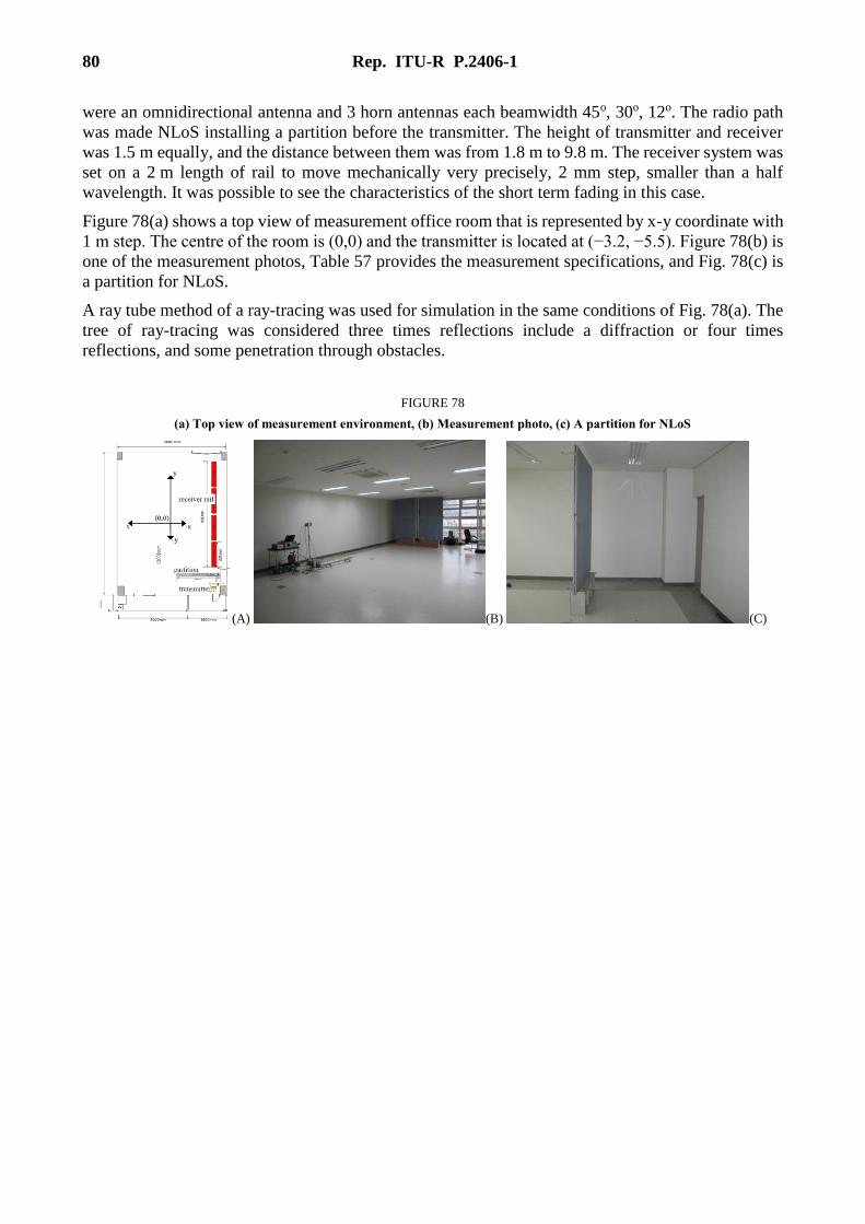
80 Rep. ITU-R P.2406-1
were an omnidirectional antenna and 3 horn antennas each beamwidth 45o, 30o, 12o. The radio path
was made NLoS installing a partition before the transmitter. The height of transmitter and receiver
was 1.5 m equally, and the distance between them was from 1.8 m to 9.8 m. The receiver system was
set on a 2 m length of rail to move mechanically very precisely, 2 mm step, smaller than a half
wavelength. It was possible to see the characteristics of the short term fading in this case.
Figure 78(a) shows a top view of measurement office room that is represented by x-y coordinate with
1 m step. The centre of the room is (0,0) and the transmitter is located at (−3.2, −5.5). Figure 78(b) is
one of the measurement photos, Table 57 provides the measurement specifications, and Fig. 78(c) is
a partition for NLoS.
A ray tube method of a ray-tracing was used for simulation in the same conditions of Fig. 78(a). The
tree of ray-tracing was considered three times reflections include a diffraction or four times
reflections, and some penetration through obstacles.
FIGURE 78
(a) Top view of measurement environment, (b) Measurement photo, (c) A partition for NLoS
(A) (B) (C)

Rep. ITU-R P.2406-1 81
TABLE 57
Measurement specifications
Tx antenna Omnidirectional antenna
Rx antennas 4 types beamwidth : omni, 45o, 30o, 12o
Distance between Tx and RX straight line, from 1.8 m to 9.8 m
(y = −3.7 ~ +4.3)
Height of Tx and Rx 1.5 m
Measurement spacing 2 mm step
Empty room size 13 × 8.6 × 3 m
6.8.4 Validation results
Figure 79(a), (b), (c), (d) with the measured and simulated results show the level of the received
signals based on distance between transmitter and receiver. They almost agree with each other and
the difference of them is represented by the rms error of equation (27).
(27)
The receive antenna of Fig. 79(a) shows a 12o beamwidth and it shows 6.8 dB of rms error.
Figure 79(b) shows a 30o beamwidth of the receive antenna and 5.8 dB of rms error. Figure 79(c)
shows a 45o beamwidth of the receiving antenna and 6.9 dB of rms error. The omni directional receive
antenna of Fig. 79(d) is 7.3 dB of rms error. Overall, the rms error distributes between the
5.8 ~ 7.3 dB, and they are a severe variation due to including the short term fading. If it were
considered as long term fading, the rms error is expected much reduced.
FIGURE 79
Comparison of measurement and simulation results:
(a) beamwidth 12 degrees, RMSE : 6.8dB, (b) beamwidth 30 degrees, RMSE : 5.8dB
(c) beamwidth 45 degrees, RMSE : 6.9dB, (d) omnidirectional antenna, RMSE : 7.3dB
(A) (B)
1, 1
2
n
ms
msRMSE
n
i
ii
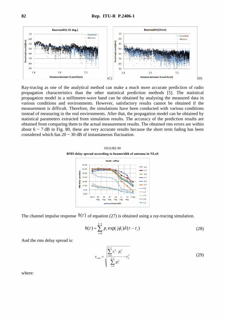
82 Rep. ITU-R P.2406-1
(C) (D)
Ray-tracing as one of the analytical method can make a much more accurate prediction of radio
propagation characteristics than the other statistical prediction methods [5]. The statistical
propagation model in a millimetre-wave band can be obtained by analysing the measured data in
various conditions and environments. However, satisfactory results cannot be obtained if the
measurement is difficult. Therefore, the simulations have been conducted with various conditions
instead of measuring in the real environments. After that, the propagation model can be obtained by
statistical parameters extracted from simulation results. The accuracy of the prediction results are
obtained from comparing them to the actual measurement results. The obtained rms errors are within
about 6 ~ 7 dB in Fig. 80, these are very accurate results because the short term fading has been
considered which has 20 ~ 30 dB of instantaneous fluctuation.
FIGURE 80
RMS delay spread according to beamwidth of antenna in NLoS
The channel impulse response of equation (27) is obtained using a ray-tracing simulation.
(28)
And the rms delay spread is:
(29)
where:
)(h
1
0
)()exp()(I
i
iii jph
2
1
0
2
1
0
22
nI
i
i
I
i
ii
rms
p
p
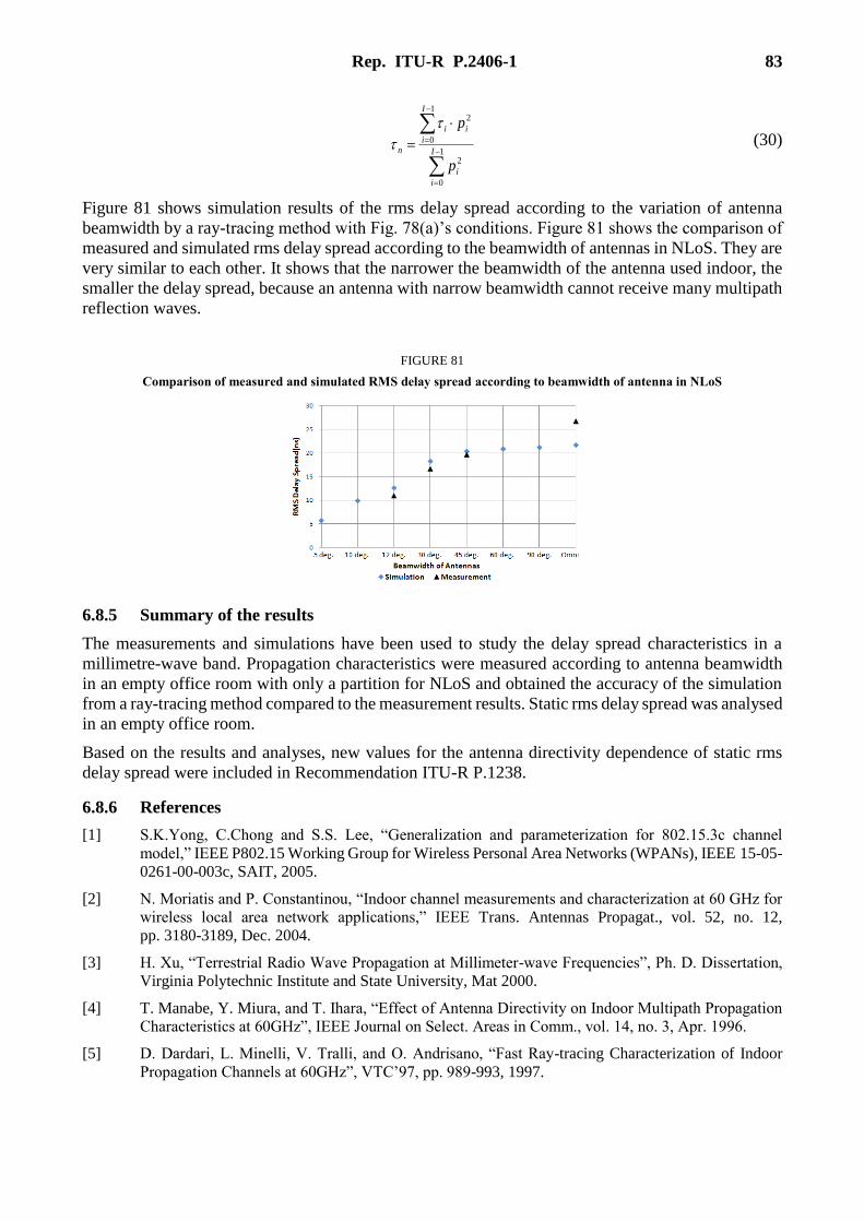
Rep. ITU-R P.2406-1 83
(30)
Figure 81 shows simulation results of the rms delay spread according to the variation of antenna
beamwidth by a ray-tracing method with Fig. 78(a)’s conditions. Figure 81 shows the comparison of
measured and simulated rms delay spread according to the beamwidth of antennas in NLoS. They are
very similar to each other. It shows that the narrower the beamwidth of the antenna used indoor, the
smaller the delay spread, because an antenna with narrow beamwidth cannot receive many multipath
reflection waves.
FIGURE 81
Comparison of measured and simulated RMS delay spread according to beamwidth of antenna in NLoS
6.8.5 Summary of the results
The measurements and simulations have been used to study the delay spread characteristics in a
millimetre-wave band. Propagation characteristics were measured according to antenna beamwidth
in an empty office room with only a partition for NLoS and obtained the accuracy of the simulation
from a ray-tracing method compared to the measurement results. Static rms delay spread was analysed
in an empty office room.
Based on the results and analyses, new values for the antenna directivity dependence of static rms
delay spread were included in Recommendation ITU-R P.1238.
6.8.6 References
[1] S.K.Yong, C.Chong and S.S. Lee, “Generalization and parameterization for 802.15.3c channel
model,” IEEE P802.15 Working Group for Wireless Personal Area Networks (WPANs), IEEE 15-05-
0261-00-003c, SAIT, 2005.
[2] N. Moriatis and P. Constantinou, “Indoor channel measurements and characterization at 60 GHz for
wireless local area network applications,” IEEE Trans. Antennas Propagat., vol. 52, no. 12,
pp. 3180-3189, Dec. 2004.
[3] H. Xu, “Terrestrial Radio Wave Propagation at Millimeter-wave Frequencies”, Ph. D. Dissertation,
Virginia Polytechnic Institute and State University, Mat 2000.
[4] T. Manabe, Y. Miura, and T. Ihara, “Effect of Antenna Directivity on Indoor Multipath Propagation
Characteristics at 60GHz”, IEEE Journal on Select. Areas in Comm., vol. 14, no. 3, Apr. 1996.
[5] D. Dardari, L. Minelli, V. Tralli, and O. Andrisano, “Fast Ray-tracing Characterization of Indoor
Propagation Channels at 60GHz”, VTC’97, pp. 989-993, 1997.
1
0
2
1
0
2
I
i
i
I
i
ii
n
p
p
84 Rep. ITU-R P.2406-1
6.9 Study 9: Effects of antenna beamwidth to multipath delay and angular spread
(Frequency bands: 28, 38 GHz)
6.9.1 Executive summary
This study observes the effect of antenna beamwidth for multipath propagation characterization in
various indoor office environments to derive coefficients of delay spread and angular spread as a
function of antenna beamwidth. Measurements were conducted at 28 GHz and 38 GHz.
6.9.2 Background and proposal
The rms delay spread DS depends on half-power beamwidth of antenna (degree):
ns (31)
where is a coefficient of rms delay spread and the range of is defined as 10o≤ ≤120o. Table 58
lists the typical values of the coefficients and a standard deviation based on each measurement
condition. The coefficients of delay spread represent cases when the boresights of antennas were
aligned to have a maximum receiving power in LoS and NLoS situations, respectively.
TABLE 58
Typical coefficients for rms delay spread
Measurement conditions
Coefficients of
rms delay
spread
f
(GHz) Environment Scenario
h1
(m)
h2
(m)
Range
(m)
Tx
beamwidth
(degree)
Rx
beamwidth
(degree)
(ns)
28
Railway
Station
LoS
8 1.5
8-80
60 10
8.25 16.11
NLoS 37.54 27.22
Airport
Terminal
LoS 8-200
7.53 15.98
NLoS 63.9 96.57
38
Railway
Station
LoS
8 1.5
8-80
40 10
4.18 4.33
NLoS 24.85 28.48
Airport
Terminal
LoS 8-200
4.46 14.13
NLoS 54.54 80.72
Office LoS
2.5 1.2 7-24 omni 10 1.16 12
NLoS 15.13 21.8
The rms angular spread AS depends on half-power beamwidth of antenna (degree):
degree (32)
where and are coefficients of rms angular spread and the range of is defined as 10o≤ ≤120o.
Table 59 lists the typical values of the coefficients and standard deviation based on each
measurement condition. The coefficients of angular spread represent cases when the boresights of
antennas are aligned to have a maximum receiving power in LoS and NLoS situations, respectively.
10log)( DS
)(AS

Rep. ITU-R P.2406-1 85
TABLE 59
Typical coefficients for rms angular spread
Measurement conditions Coefficients of rms
angular spread
f
(GHz) Environment Scenario
h1
(m)
h2
(m)
Range
(m)
Tx
beam-
width
(degree)
Rx
beam-
width
(degree)
(degree)
28
Railway
Station
LoS
8 1.5
8-80
60 10
0.5 0.77 2.3
NLoS 0.25 1.0 2.32
Airport
Terminal
LoS 8-200
1.2 0.49 2.18
NLoS 0.3 0.96 3.12
38
Railway
Station
LoS
8 1.5
8-80
40 10
1.14 0.54 3.36
NLoS 0.16 1.1 3.24
Airport
Terminal
LoS 8-200
2.0 0.34 1.36
NLoS 0.34 0.93 2.99
Office LoS
2.5 1.2 7-24 omni 10 0.07 1.22 5.58
NLoS 0.17 1.07 4.81
6.9.3 Measurement setup and procedure
6.9.3.1 Measurement equipment
Table 60 lists a detailed specification of the ETRI’s channel sounder measuring the spatial and
temporal characteristics of a 500 MHz wideband channel at the centre frequencies of 28 and 38 GHz
[4]. As shown in Fig. 82, the positioner can mount a directional horn antenna and can rotate the
orientation of the horn antenna both horizontally and vertically with 1° accuracy to control the bore-
sight of transmitting/receiving beams during measurements.
TABLE 60
Specifications of ETRI’s channel sounder
System parameters Specifications
Centre frequency 28/38 GHz
Channel Bandwidth 500 MHz
PN code length of probing signal 4095 chips
Maximum TX power
(w/o antenna)
28 GHz 29 dBm
38 GHz 21 dBm
Multipath resolution 2 ns
HPBW of pyramidal horn
antenna and gain
28 GHz 10o(24.4 dBi), 60o (9.9 dBi)
38 GHz 10o(24.6 dBi), 40o (12.6 dBi)
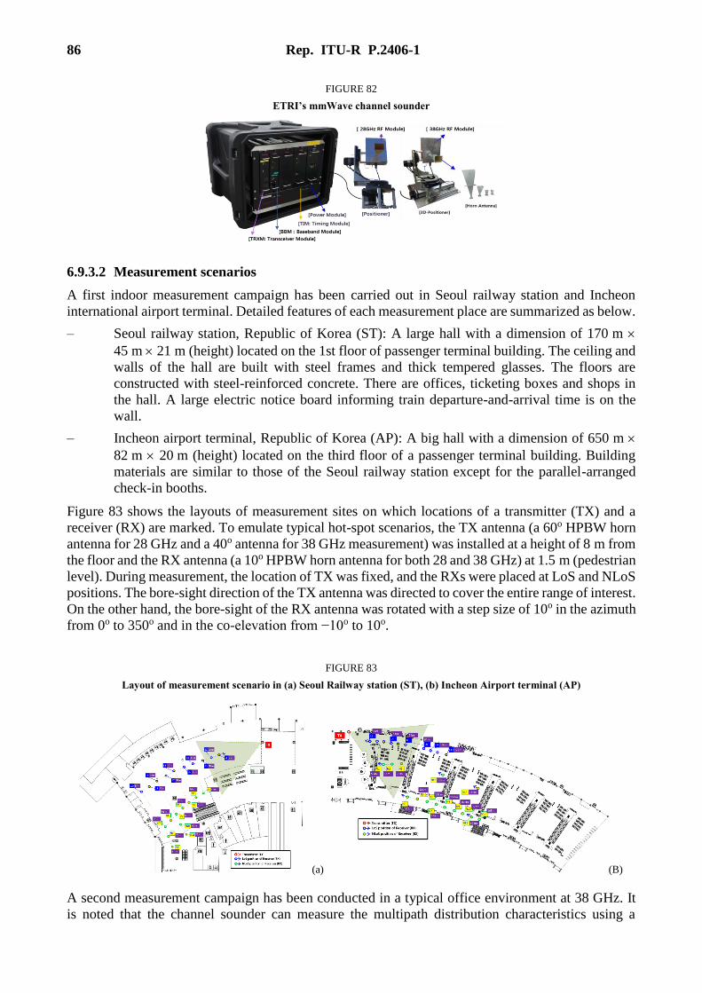
86 Rep. ITU-R P.2406-1
FIGURE 82
ETRI’s mmWave channel sounder
6.9.3.2 Measurement scenarios
A first indoor measurement campaign has been carried out in Seoul railway station and Incheon
international airport terminal. Detailed features of each measurement place are summarized as below.
– Seoul railway station, Republic of Korea (ST): A large hall with a dimension of 170 m
45 m 21 m (height) located on the 1st floor of passenger terminal building. The ceiling and
walls of the hall are built with steel frames and thick tempered glasses. The floors are
constructed with steel-reinforced concrete. There are offices, ticketing boxes and shops in
the hall. A large electric notice board informing train departure-and-arrival time is on the
wall.
– Incheon airport terminal, Republic of Korea (AP): A big hall with a dimension of 650 m
82 m 20 m (height) located on the third floor of a passenger terminal building. Building
materials are similar to those of the Seoul railway station except for the parallel-arranged
check-in booths.
Figure 83 shows the layouts of measurement sites on which locations of a transmitter (TX) and a
receiver (RX) are marked. To emulate typical hot-spot scenarios, the TX antenna (a 60o HPBW horn
antenna for 28 GHz and a 40o antenna for 38 GHz measurement) was installed at a height of 8 m from
the floor and the RX antenna (a 10o HPBW horn antenna for both 28 and 38 GHz) at 1.5 m (pedestrian
level). During measurement, the location of TX was fixed, and the RXs were placed at LoS and NLoS
positions. The bore-sight direction of the TX antenna was directed to cover the entire range of interest.
On the other hand, the bore-sight of the RX antenna was rotated with a step size of 10o in the azimuth
from 0o to 350o and in the co-elevation from −10o to 10o.
FIGURE 83
Layout of measurement scenario in (a) Seoul Railway station (ST), (b) Incheon Airport terminal (AP)
(a) (B)
A second measurement campaign has been conducted in a typical office environment at 38 GHz. It
is noted that the channel sounder can measure the multipath distribution characteristics using a
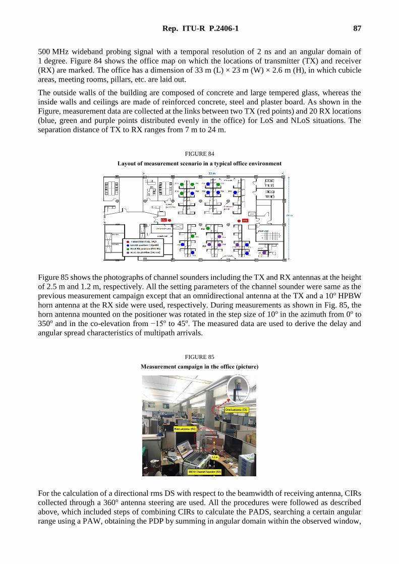
Rep. ITU-R P.2406-1 87
500 MHz wideband probing signal with a temporal resolution of 2 ns and an angular domain of
1 degree. Figure 84 shows the office map on which the locations of transmitter (TX) and receiver
(RX) are marked. The office has a dimension of 33 m (L) × 23 m (W) × 2.6 m (H), in which cubicle
areas, meeting rooms, pillars, etc. are laid out.
The outside walls of the building are composed of concrete and large tempered glass, whereas the
inside walls and ceilings are made of reinforced concrete, steel and plaster board. As shown in the
Figure, measurement data are collected at the links between two TX (red points) and 20 RX locations
(blue, green and purple points distributed evenly in the office) for LoS and NLoS situations. The
separation distance of TX to RX ranges from 7 m to 24 m.
FIGURE 84
Layout of measurement scenario in a typical office environment
Figure 85 shows the photographs of channel sounders including the TX and RX antennas at the height
of 2.5 m and 1.2 m, respectively. All the setting parameters of the channel sounder were same as the
previous measurement campaign except that an omnidirectional antenna at the TX and a 10o HPBW
horn antenna at the RX side were used, respectively. During measurements as shown in Fig. 85, the
horn antenna mounted on the positioner was rotated in the step size of 10o in the azimuth from 0o to
350o and in the co-elevation from −15o to 45o. The measured data are used to derive the delay and
angular spread characteristics of multipath arrivals.
FIGURE 85
Measurement campaign in the office (picture)
For the calculation of a directional rms DS with respect to the beamwidth of receiving antenna, CIRs
collected through a 360o antenna steering are used. All the procedures were followed as described
above, which included steps of combining CIRs to calculate the PADS, searching a certain angular
range using a PAW, obtaining the PDP by summing in angular domain within the observed window,
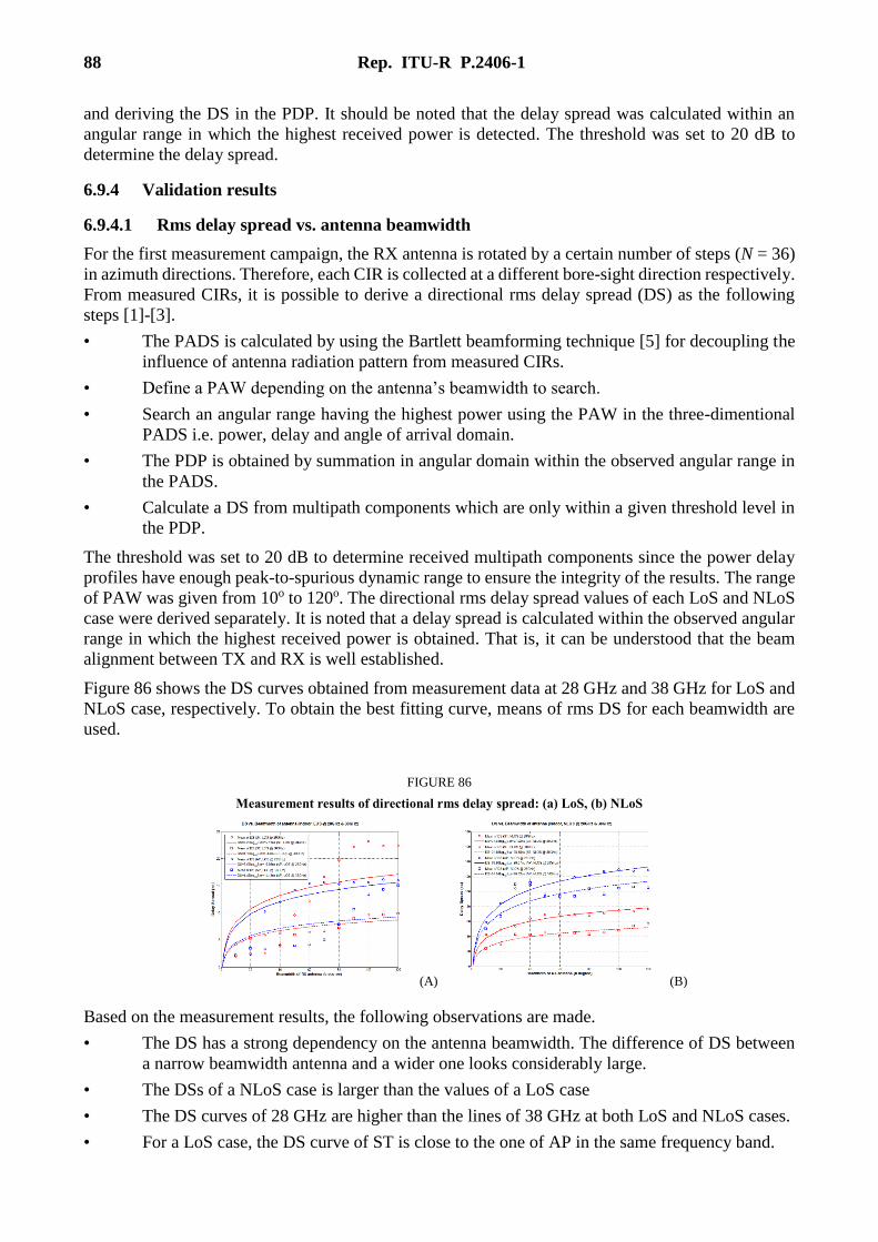
88 Rep. ITU-R P.2406-1
and deriving the DS in the PDP. It should be noted that the delay spread was calculated within an
angular range in which the highest received power is detected. The threshold was set to 20 dB to
determine the delay spread.
6.9.4 Validation results
6.9.4.1 Rms delay spread vs. antenna beamwidth
For the first measurement campaign, the RX antenna is rotated by a certain number of steps (N = 36)
in azimuth directions. Therefore, each CIR is collected at a different bore-sight direction respectively.
From measured CIRs, it is possible to derive a directional rms delay spread (DS) as the following
steps [1]-[3].
• The PADS is calculated by using the Bartlett beamforming technique [5] for decoupling the
influence of antenna radiation pattern from measured CIRs.
• Define a PAW depending on the antenna’s beamwidth to search.
• Search an angular range having the highest power using the PAW in the three-dimentional
PADS i.e. power, delay and angle of arrival domain.
• The PDP is obtained by summation in angular domain within the observed angular range in
the PADS.
• Calculate a DS from multipath components which are only within a given threshold level in
the PDP.
The threshold was set to 20 dB to determine received multipath components since the power delay
profiles have enough peak-to-spurious dynamic range to ensure the integrity of the results. The range
of PAW was given from 10o to 120o. The directional rms delay spread values of each LoS and NLoS
case were derived separately. It is noted that a delay spread is calculated within the observed angular
range in which the highest received power is obtained. That is, it can be understood that the beam
alignment between TX and RX is well established.
Figure 86 shows the DS curves obtained from measurement data at 28 GHz and 38 GHz for LoS and
NLoS case, respectively. To obtain the best fitting curve, means of rms DS for each beamwidth are
used.
FIGURE 86
Measurement results of directional rms delay spread: (a) LoS, (b) NLoS
(A) (B)
Based on the measurement results, the following observations are made.
• The DS has a strong dependency on the antenna beamwidth. The difference of DS between
a narrow beamwidth antenna and a wider one looks considerably large.
• The DSs of a NLoS case is larger than the values of a LoS case
• The DS curves of 28 GHz are higher than the lines of 38 GHz at both LoS and NLoS cases.
• For a LoS case, the DS curve of ST is close to the one of AP in the same frequency band.

Rep. ITU-R P.2406-1 89
• For a NLoS case, the DS curves of AP are seen as higher than ST. It means that multipath
components in AP are more widespread in the delay domain than the circumstance of ST. It
is noted that the hall size of AP is bigger than the ST.
The rms delay spread DS with respect to which follows a normal distribution with the standard
deviation is given by;
ns (33)
where the range of is defined as 0o≤ ≤120o.
Table 61 summarizes the typical coefficients of DS model and standard deviation for each
measurement scenario and frequency band.
TABLE 61
Directional rms delay spread parameters
Indoor environments
rms delay spread (ns)
(ns)
Railway Station (ST) 28GHz LoS 8.25 16.11
NLoS 37.54 27.22
38GHz LoS 4.18 4.33
NLoS 24.85 28.48
Airport Terminal (AP) 28GHz LoS 7.53 15.98
NLoS 63.9 96.57
38GHz LoS 4.46 14.13
NLoS 54.54 80.72
For the second measurement campaign, for the calculation of a directional rms DS with respect to the
beamwidth of receiving antenna, CIRs collected through a 360o antenna steering are used. All the
procedures of the first campaign were followed, which include steps of combining CIRs to calculate
the PADS, searching a certain angular range using a PAW, obtaining the PDP by summing in angular
domain within the observed window, and deriving the DS in the PDP. It should be noted that the
delay spread was calculated within an angular range in which the highest received power is detected.
The threshold was set to 20 dB to determine the delay spread. Figure 87 shows the DS curves for LoS
and NLoS cases.
10log)( DS

90 Rep. ITU-R P.2406-1
FIGURE 87
Measurement results of rms delay spread for LoS and NLoS (office at 38 GHz)
Based on the measurement results in a typical office environment at 38 GHz, the following
observations are made.
– The DS has a strong dependency on the antenna beamwidth. The wider beamwidth has the
larger DS.
– The DSs at NLoS case is larger than those of LoS case.
– These properties are very similar to the measurement results in commercial environments at
28 and 38 GHz
Table 62 summarizes the typical coefficients of DS model and a standard deviation for LoS and
NLoS situations, respectively, in a typical indoor office environment.
TABLE 62
rms delay spread parameters
Indoor environments rms delay spread (ns)
(ns)
Office 38 GHz LoS 10.16 12
NLoS 15.13 21.8
6.9.4.2 Rms angular spread vs. antenna beamwidth
For the first measurement campaign, the rms AS can be easily derived from the PAS. The PAS is
calculated from the PADS by summation in delay domain [1]-[3]. To calculate the directional rms
AS, the threshold level was set to 20 dB. Figure 88(a) and (b) show the AS curves which were
obtained from measurement data at 28 and 38 GHz for LoS and NLoS cases, respectively. To derive
the best fitting curve, mean values of AS for each beamwidth are used.

Rep. ITU-R P.2406-1 91
FIGURE 88
Measurement results of directional rms angular spread: (a) LoS, (b) NLoS
(A) (B)
From measurement results, the following can be observed:
– The AS shows a strong dependency on the antenna beamwidth as similar to the DS. The
wider beamwidth of the antenna is the larger angular spread.
– For the LoS case, the AS of 28 GHz is higher than the curve of 38 GHz. However, the
frequency dependency is not seen in case of NLoS.
– For the NLoS case, the angular spread continuously increase from narrow to wider
beamwidths.
– For the LoS case, the AS values of ST are larger than the AP environment. On the other hand,
the values of ST and AP are similar in case of NLoS. The multipath components in AP are
more spread in the delay domain but the spread in angular domain is similar to the
circumstance of ST.
The rms angular spread AS with respect to which follows a normal distribution with the standard
deviation is given by;
degree (34)
where the range of is defined as 0o≤ ≤120o.
The typical coefficients of angular spread model AS and standard deviation for each measurement
scenario and frequency band are summarized in Table 63.
)(AS

92 Rep. ITU-R P.2406-1
TABLE 63
Directional rms angular spread parameters
Indoor environments rms angular spread (degree)
(o)
Railway Station
(ST)
28 GHz LoS 0.5 0.77 2.3
NLoS 0.25 1.0 2.32
38 GHz LoS 1.14 0.54 3.36
NLoS 0.16 1.1 3.24
Airport Terminal
(AP)
28 GHz LoS 1.2 0.49 2.18
NLoS 0.3 0.96 3.12
38 GHz LoS 2.0 0.34 1.36
NLoS 0.34 0.93 2.99
For the second measurement campaign, the rms AS depending on the antenna’s beamwidth is derived
using the same methods as in the first campaign. To calculate the directional rms AS, the threshold
level was set to 20 dB. Figure 89 shows the AS curves which are obtained from measurement data at
38 GHz for LoS and NLoS situations, respectively.
FIGURE 89
Measurement results of rms angular spread for LoS and NLoS (office at 38 GHz)
From measurement results, it can be observed the following properties.
– The AS shows a strong dependency on the antenna beamwidth as similar to the DS. When
the beamwidth of RX antenna is wider, the larger angular spread is observed.
– For the NLoS case, the angular spread monotonically increases as beamwidth increases.
– These properties are very similar to the measurement results in commercial environments at
28 and 38 GHz.
Table 64 summarizes the typical coefficients of AS model and a standard deviation for LoS and
NLoS situations, respectively, in a typical indoor office environment.
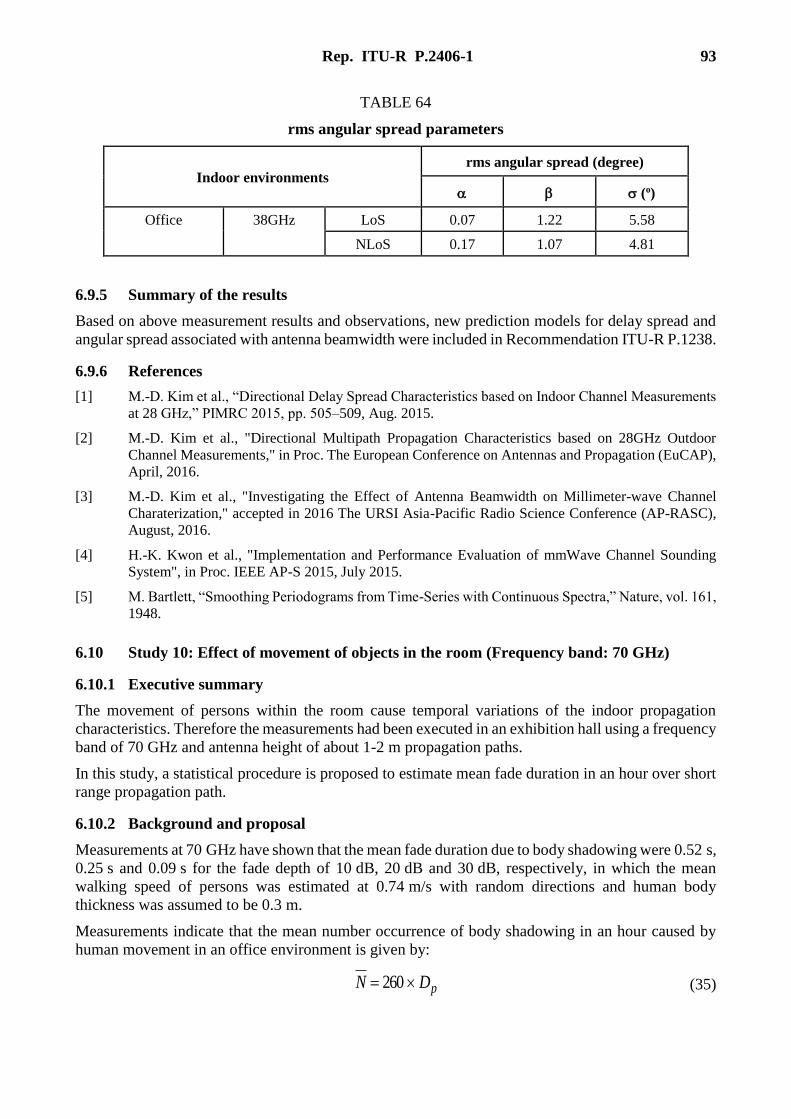
Rep. ITU-R P.2406-1 93
TABLE 64
rms angular spread parameters
Indoor environments rms angular spread (degree)
(o)
Office 38GHz LoS 0.07 1.22 5.58
NLoS 0.17 1.07 4.81
6.9.5 Summary of the results
Based on above measurement results and observations, new prediction models for delay spread and
angular spread associated with antenna beamwidth were included in Recommendation ITU-R P.1238.
6.9.6 References
[1] M.-D. Kim et al., “Directional Delay Spread Characteristics based on Indoor Channel Measurements
at 28 GHz,” PIMRC 2015, pp. 505–509, Aug. 2015.
[2] M.-D. Kim et al., "Directional Multipath Propagation Characteristics based on 28GHz Outdoor
Channel Measurements," in Proc. The European Conference on Antennas and Propagation (EuCAP),
April, 2016.
[3] M.-D. Kim et al., "Investigating the Effect of Antenna Beamwidth on Millimeter-wave Channel
Charaterization," accepted in 2016 The URSI Asia-Pacific Radio Science Conference (AP-RASC),
August, 2016.
[4] H.-K. Kwon et al., "Implementation and Performance Evaluation of mmWave Channel Sounding
System", in Proc. IEEE AP-S 2015, July 2015.
[5] M. Bartlett, “Smoothing Periodograms from Time-Series with Continuous Spectra,” Nature, vol. 161,
1948.
6.10 Study 10: Effect of movement of objects in the room (Frequency band: 70 GHz)
6.10.1 Executive summary
The movement of persons within the room cause temporal variations of the indoor propagation
characteristics. Therefore the measurements had been executed in an exhibition hall using a frequency
band of 70 GHz and antenna height of about 1-2 m propagation paths.
In this study, a statistical procedure is proposed to estimate mean fade duration in an hour over short
range propagation path.
6.10.2 Background and proposal
Measurements at 70 GHz have shown that the mean fade duration due to body shadowing were 0.52 s,
0.25 s and 0.09 s for the fade depth of 10 dB, 20 dB and 30 dB, respectively, in which the mean
walking speed of persons was estimated at 0.74 m/s with random directions and human body
thickness was assumed to be 0.3 m.
Measurements indicate that the mean number occurrence of body shadowing in an hour caused by
human movement in an office environment is given by:
(35) pDN 260

94 Rep. ITU-R P.2406-1
where Dp (0.05 < Dp < 0.08) is the number of persons per square metre in the room. The total fade
duration per hour is then given by:
(36)
where is mean fade duration.
6.10.3 Measurement setup and procedure
The measurement of propagation characteristics was carried out in an exhibition hall, and investigated
the characteristic of the shadowing loss due to human movement. Figure 90 shows a measurement
layout in an exhibition hall. Table 65 shows measurement conditions. The width of this hall was 22 m
times 13 m with wooden inner walls [1]. A vector network analyser (VNA) was used in order to
measure propagation loss. Propagation path was set in front of exhibition booths. The transmitting
frequency was set at 70.0 GHz, and a carrier wave (CW) was transmitted. The instantaneous variation
of the received level was measured for several transmitting antenna heights and propagation
distances.
FIGURE 90
A measurement layout in an exhibition hall
TABLE 65
Measurement conditions
Frequency 70.0 GHz (CW)
Polarization Vertical
Antenna
(3 dB beam width)
Wave Guide Horn
(15 degrees)
Antenna height Tx 1.05 m, 2.05 m
Rx 1.05 m
Propagation Distance 3.3 m, 7.3 m, 10.8 m
6.10.4 Validation results
6.10.4.1 Characteristics of cumulative probability distributions of attenuation level
Figure 91(a) shows cumulative probability distributions of attenuation level measured for several
propagation distances when a person crossed the path at a speed of about 1 m/s.
NTT s
sT
ht
d
hr
Tx Antenna
Rx Antenna

Rep. ITU-R P.2406-1 95
Figure 91(b) shows cumulative probability distributions of attenuation level measured for several
transmitting antenna heights.
FIGURE 91
Cumulative probability distributions of attenuation level measured for:
(a) several propagation distances, (b) several transmitting antenna heights
(A) (B)
6.10.4.2 Investigation of mean fade duration
Variations of mean fade durations versus attenuation level are shown in Fig. 92(a). This Figure shows
measured results when the transmitting antenna height was fixed at 2.05 m. According to Fig. 92(a),
the fade duration becomes longer in 3.3 m path in comparison with other paths. This is because the
attenuation had occurred in the limited area near the receiving antenna.
Variations of mean fade durations versus attenuation level when each transmitting antenna height was
fixed at 1.05 m and 2.05 m are shown in Fig. 92(b). The mean fade duration decreased gradually in
proportion with the attenuation level. Furthermore variations of mean fade duration became small in
the range of more than 25 dB. For example, when the attenuation level is 16.4 dB, the mean fade
duration was estimated about 0.35 s from Fig. 92(b). The mean fade duration at 70.0 GHz when the
attenuation level was 10 dB, 20 dB, and 30 dB then the fade duration was 0.52 s, 0.25s, and 0.09 s,
respectively. According to the measurement results at 37 GHz in an indoor office environment
reported in Recommendation ITU-R P.1238, at a fade depth of 10 dB, the mean fade duration was
0.11 s and at a fade depth of 15 dB, the mean duration was 0.05 s.
FIGURE 92
Variation of mean fade durations: (a) ht=2.05 m, (b) ht=1.05 m, 2.05 m
(A) (B)
60 50 40 30 20 10 0
.01
.1
1
5102030
50
70809095
99
99.9
99.99
d=3.3md=7.3md=10.8m
Attenuation level (dB)
Cu
mu
lati
ve
pro
bab
ilit
y (
%)
Frequency:70.0GHz
ht:1.05m, 2.05m
hr:1.05m
Ant.:Horn(15degrees)
Polarization:Vertical
60 50 40 30 20 10 0.01
.1
1
5102030
50
70809095
99
99.9
99.99
ht=1.05mht=2.05mAveraged
Attenuation level (dB)C
um
ula
tiv
e p
rob
abil
ity
(%
)
Frequency:70.0GHz
hr:1.05m
d:3.3m, 7.3m, 10.8m
Ant.:Horn(15degrees)
Polarization:Vertical
0
0.2
0.4
0.6
0.8
1
0 10 20 30 40 50
d=3.3m
d=7.3m
d=10.8m
Mea
n f
ade
dura
tion
(s)
Attenuation level (dB)
Frequency:70.0GHz
ht:2.05m, hr:1.05m
Ant.:Horn(15degrees)
Polarization:Vertical
0
0.2
0.4
0.6
0.8
1
0 10 20 30 40 50
d=3.3m
d=7.3m
d=10.8m
Averaged
Mea
n f
ade
du
rati
on
(s)
Attenuation level (dB)
Frequency:70.0GHz
ht:1.05m, 2.05m
hr:1.05m
Ant.:Horn(15degrees)
Polarization:Vertical

96 Rep. ITU-R P.2406-1
6.10.4.3 Characteristics of human movement
In order to presume the total amount of fade duration per hour, it is necessary to describe not only the
mean fade duration but also the characteristics of human movement in the actual environment.
6.10.4.3.1 Measurement procedure
The investigation was carried out in two different sized offices. A sample of propagation path layout
in the office is shown in Fig. 93. The 2 or 3 LoS paths were set in each office, and the number of each
path interruption occurrence was investigated. The measurement was carried out from 8:30 to 17:00.
FIGURE 93
A sample of propagation path layout in the office
6.10.4.3.2 Measurement results of human movement
The number of path interruption occurrence (N) when people cross the propagation path in an hour
is shown in Fig. 94. A horizontal axis indicates a density of population per one square meter. In this
Figure, N of 57 was measured at lunchtime. Although there was variation by measurement time zone,
the N increased gradually in proportion with density of population per one square meter (Dp).
In Fig. 94, a regression curve is shown and it is expressed as follows.
(37)
Here, 0.05 < Dp < 0.08.
FIGURE 94
Characteristics of the number interruption occurrence per hour
★
Path A
Path B
DpN 260
0
10
20
30
40
50
60
0 0.02 0.04 0.06 0.08 0.1
measured dataN=260Dp
Th
e n
um
ber
of
inte
rru
pti
on
occ
urr
ence
Density of population per one square meter

Rep. ITU-R P.2406-1 97
6.10.4.4 Estimated total amount of fade duration per hour
It was proposed that a total amount of fade duration per hour (T) was estimated by using density of
population and the number of fade occurrence. The T was expressed as follows.
(38)
Where, T is a total amount of fade duration per hour in seconds, Ts_ave is the mean fade duration in
second, and N is the number of fade occurrence per hour.
6.10.5 Summary of the results
Propagation measurements were carried out in actual circumstances where humans randomly moved,
in order to design a millimetre-wave ad-hoc wireless access system. In addition to characteristics of
shadowing loss, characteristics of fade duration were analysed. Furthermore, human movement was
observed in offices, the relations between the number of path interruption occurrences and the density
of population per one square meter was derived. As a result, it was possible to estimate the total
amount of fade duration per hour by using the statistical function of attenuation level and density of
population per one square meter.
6.10.6 References
[1] F. Ohkubo, et al., “Millimeter-Wave Ad-Hoc Wireless Access System II- (5) Statistical
Characteristics of Shadowing Loss due to Human Movement-”, TSMMW2003, Mar. 2003.
6.11 Study 11: Power loss coefficients (Frequency bands: 250-325 GHz)
6.11.1 Executive summary
This section provides power loss coefficients which are based on measurements in indoor office and
corridor environments in the frequency band from 250 to 325 GHz.
6.11.2 Background and proposal
Table 66 shows the proposed power loss coefficients.
TABLE 66
Power loss coefficients, N, for indoor transmission loss calculation
Frequency
(GHz) Residential Office Commercial Factory Corridor
Data
Centre
≈
250 20.1(16) 19.0(9, 16)
275 20(16) 19.2(9, 16)
300 – 20(15)
20(17)
– – 19.5(9, 15)
18.9(9, 17)
20.2(15)
325 19.8(17) 19.6(9, 17)
(9) Transmitter and receiver are on LoS corridor.
(15) Transmit and received antennas have 10° beamwidth.
(16) Transmit and received antennas have 8° beamwidth.
(17) Transmit and received antennas have 7° beamwidth.
NaveTsT _
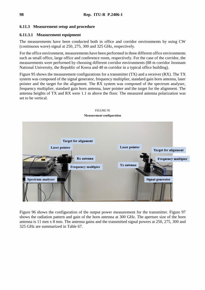
98 Rep. ITU-R P.2406-1
6.11.3 Measurement setup and procedure
6.11.3.1 Measurement equipment
The measurements have been conducted both in office and corridor environments by using CW
(continuous wave) signal at 250, 275, 300 and 325 GHz, respectively.
For the office environment, measurements have been performed in three different office environments
such as small office, large office and conference room, respectively. For the case of the corridor, the
measurements were performed by choosing different corridor environments (88 m corridor Jeonnam
National University, the Republic of Korea and 48 m corridor in a typical office building).
Figure 95 shows the measurement configurations for a transmitter (TX) and a receiver (RX). The TX
system was composed of the signal generator, frequency multiplier, standard gain horn antenna, laser
pointer and the target for the alignment. The RX system was composed of the spectrum analyser,
frequency multiplier, standard gain horn antenna, laser pointer and the target for the alignment. The
antenna heights of TX and RX were 1.1 m above the floor. The measured antenna polarization was
set to be vertical.
FIGURE 95
Measurement configuration
Figure 96 shows the configuration of the output power measurement for the transmitter. Figure 97
shows the radiation pattern and gain of the horn antenna at 300 GHz. The aperture size of the horn
antenna is 11 mm x 8 mm. The antenna gains and the transmitted signal powers at 250, 275, 300 and
325 GHz are summarized in Table 67.
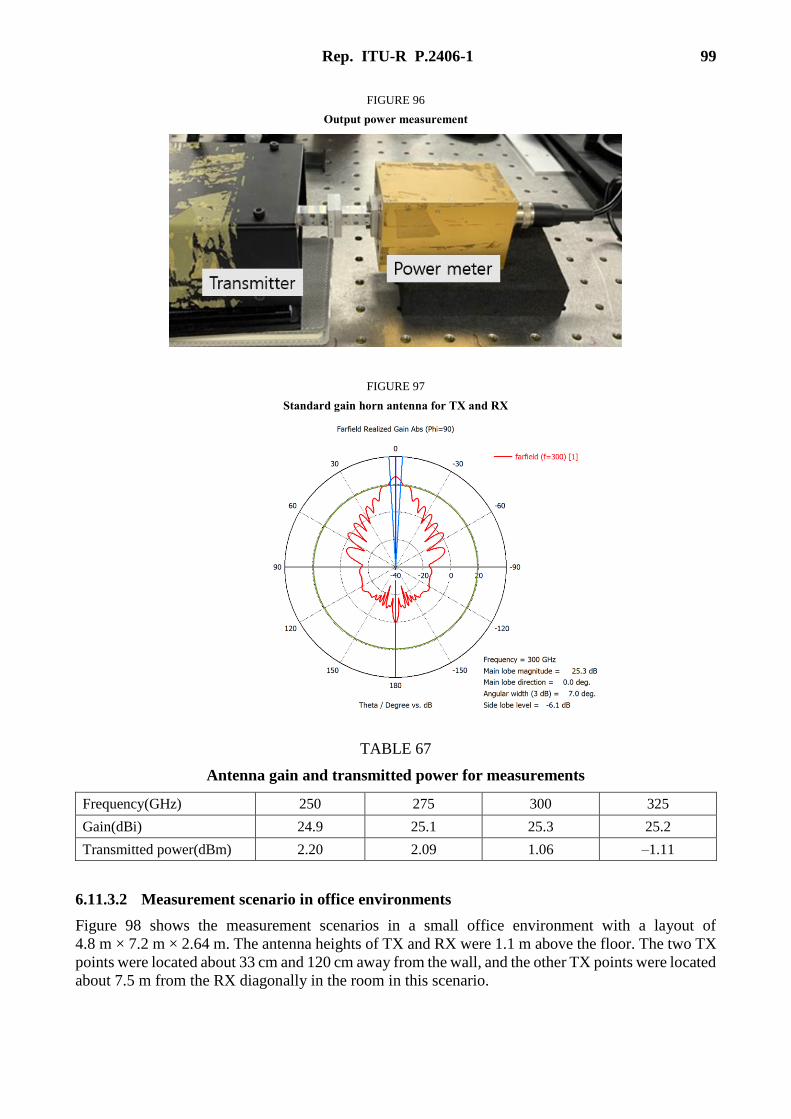
Rep. ITU-R P.2406-1 99
FIGURE 96
Output power measurement
FIGURE 97
Standard gain horn antenna for TX and RX
TABLE 67
Antenna gain and transmitted power for measurements
Frequency(GHz) 250 275 300 325
Gain(dBi) 24.9 25.1 25.3 25.2
Transmitted power(dBm) 2.20 2.09 1.06 –1.11
6.11.3.2 Measurement scenario in office environments
Figure 98 shows the measurement scenarios in a small office environment with a layout of
4.8 m × 7.2 m × 2.64 m. The antenna heights of TX and RX were 1.1 m above the floor. The two TX
points were located about 33 cm and 120 cm away from the wall, and the other TX points were located
about 7.5 m from the RX diagonally in the room in this scenario.

100 Rep. ITU-R P.2406-1
FIGURE 98
Measurement scenarios in a small office environment
(a) Measurement environment
(b) Installation of the measurement equipment
Figure 99 shows the measurement scenario in a large office environment with a layout of 12 m ×18 m
× 3 m. The antenna heights of TX and RX were 1.1 m above the floor. For the LoS case, the maximum
distance between TX and RX was 15 m in this scenario.

Rep. ITU-R P.2406-1 101
FIGURE 99
Measurement scenarios in a large office environment
(a) Measurement environment
(b) Installation of the measurement equipment
Figure 100 shows the measurement scenario in a conference room with a layout of 9 m × 11 m × 3 m.
The conference room has many desks and chairs. The antenna heights of TX and RX were 1.1 m
above the floor. For the LoS case, the maximum distance between TX and RX was 10 m in this
scenario.
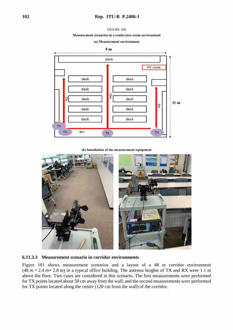
102 Rep. ITU-R P.2406-1
FIGURE 100
Measurement scenarios in a conference room environment
(a) Measurement environment
(b) Installation of the measurement equipment
6.11.3.3 Measurement scenario in corridor environments
Figure 101 shows measurement scenarios and a layout of a 48 m corridor environment
(48 m × 2.4 m× 2.8 m) in a typical office building. The antenna heights of TX and RX were 1.1 m
above the floor. Two cases are considered in this scenario. The first measurements were performed
for TX points located about 50 cm away from the wall, and the second measurements were performed
for TX points located along the centre (120 cm from the wall) of the corridor.

Rep. ITU-R P.2406-1 103
FIGURE 101
Measurement scenarios in a 48 m corridor environment
(a) Measurement environment
(b) Installation of the measurement equipment
Figure 102 shows measurement scenarios and a layout of an 88 m corridor environment
(88 m × 2.7 m × 2.9 m) at Jeonnam National University, the Republic of Korea. The first
measurements were performed for TX points located about 30 cm away from the wall, and the second
measurements were performed for TX points located along the centre (135 cm from the wall) of
corridor.
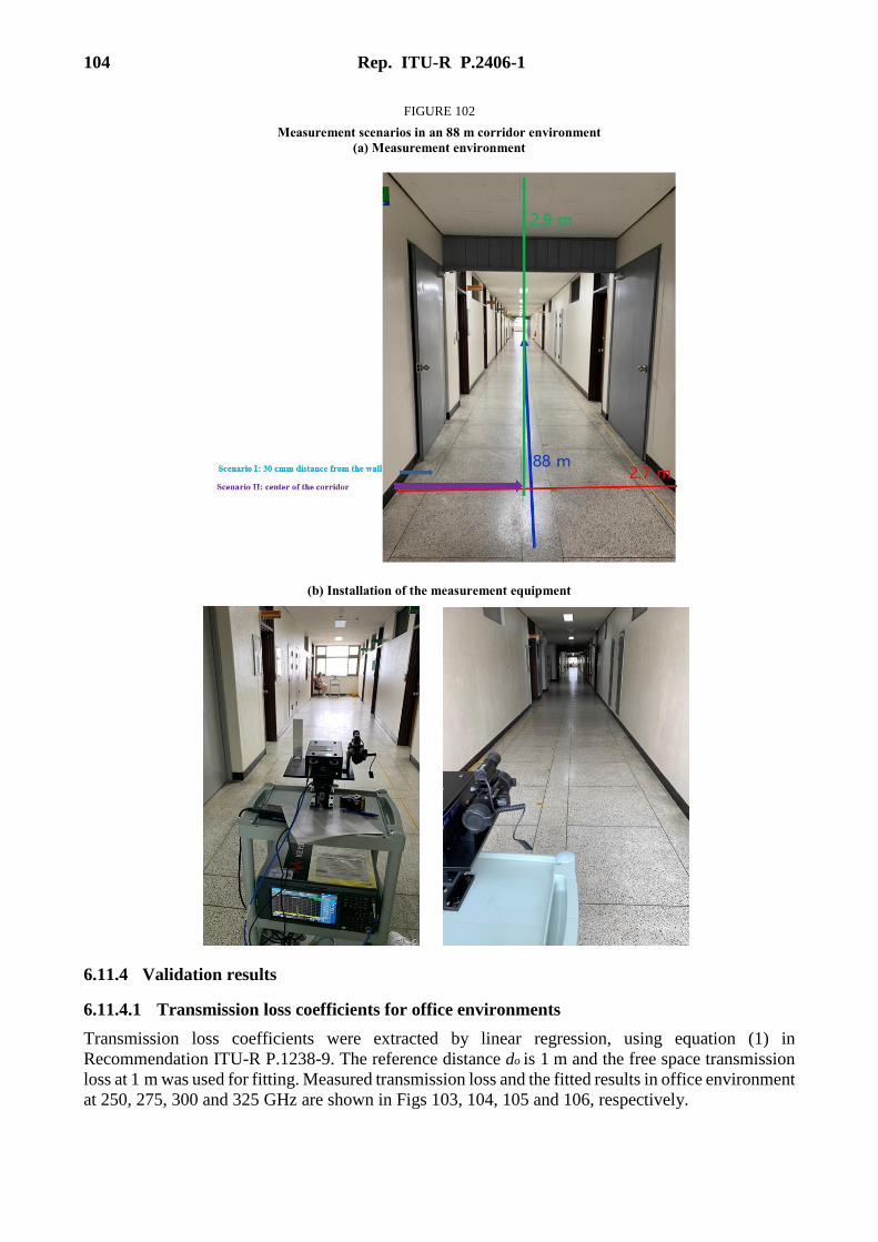
104 Rep. ITU-R P.2406-1
FIGURE 102
Measurement scenarios in an 88 m corridor environment
(a) Measurement environment
(b) Installation of the measurement equipment
6.11.4 Validation results
6.11.4.1 Transmission loss coefficients for office environments
Transmission loss coefficients were extracted by linear regression, using equation (1) in
Recommendation ITU-R P.1238-9. The reference distance do is 1 m and the free space transmission
loss at 1 m was used for fitting. Measured transmission loss and the fitted results in office environment
at 250, 275, 300 and 325 GHz are shown in Figs 103, 104, 105 and 106, respectively.

Rep. ITU-R P.2406-1 105
FIGURE 103
Transmission loss measurement results in office environments at 250 GHz
FIGURE 104
Transmission loss measurement results in office environments at 275 GHz

106 Rep. ITU-R P.2406-1
FIGURE 105
Transmission loss measurement results in office environments at 300 GHz
FIGURE 106
Transmission loss measurement results in office environments at 325 GHz
6.11.4.2 Transmission loss coefficients for corridor environments
Transmission loss coefficients were extracted by linear regression as in the office environment.
Measured transmission loss and the fitted results in office environment at 250, 275, 300 and 325 GHz
are shown in Figs 107, 108, 109 and 110, respectively.
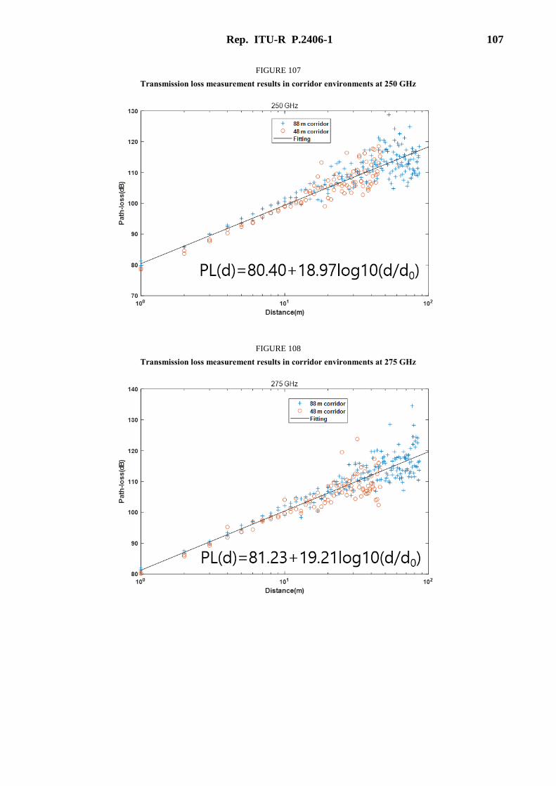
Rep. ITU-R P.2406-1 107
FIGURE 107
Transmission loss measurement results in corridor environments at 250 GHz
FIGURE 108
Transmission loss measurement results in corridor environments at 275 GHz
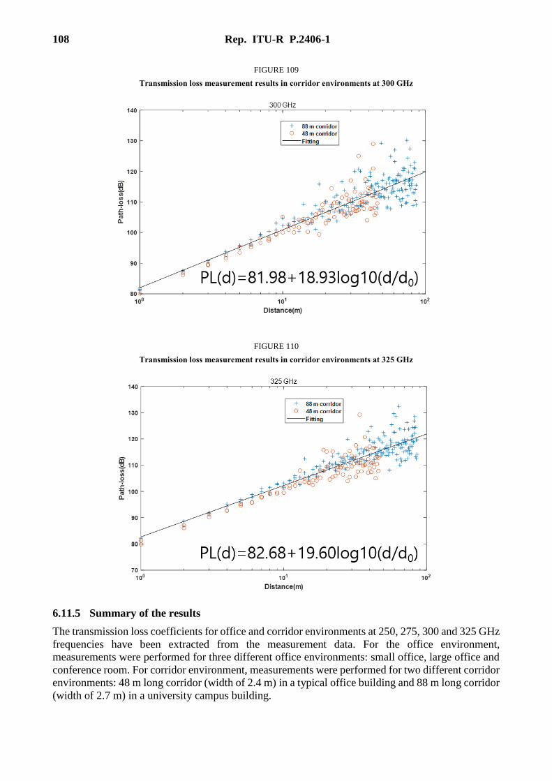
108 Rep. ITU-R P.2406-1
FIGURE 109
Transmission loss measurement results in corridor environments at 300 GHz
FIGURE 110
Transmission loss measurement results in corridor environments at 325 GHz
6.11.5 Summary of the results
The transmission loss coefficients for office and corridor environments at 250, 275, 300 and 325 GHz
frequencies have been extracted from the measurement data. For the office environment,
measurements were performed for three different office environments: small office, large office and
conference room. For corridor environment, measurements were performed for two different corridor
environments: 48 m long corridor (width of 2.4 m) in a typical office building and 88 m long corridor
(width of 2.7 m) in a university campus building.
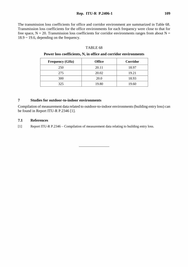
Rep. ITU-R P.2406-1 109
The transmission loss coefficients for office and corridor environment are summarized in Table 68.
Transmission loss coefficients for the office environments for each frequency were close to that for
free space, N = 20. Transmission loss coefficients for corridor environments ranges from about N =
18.9 ~ 19.6, depending on the frequency.
TABLE 68
Power loss coefficients, N, in office and corridor environments
Frequency (GHz) Office Corridor
250 20.11 18.97
275 20.02 19.21
300 20.0 18.93
325 19.80 19.60
7 Studies for outdoor-to-indoor environments
Compilation of measurement data related to outdoor-to-indoor environments (building entry loss) can
be found in Report ITU-R P.2346 [1].
7.1 References
[1] Report ITU-R P.2346 ‒ Compilation of measurement data relating to building entry loss.
________________