student's z, t, and s: what if gosset had r? · introductiontheorysimulationsaftermath /...
TRANSCRIPT

Introduction Theory Simulations AfterMath / Fisher / z → t Messages
Student’s z, t , and s: What if Gosset had R?
James A. Hanley1 Marilyse Julien2 Erica E. M. Moodie1
1Department of Epidemiology, Biostatistics and Occupational Health,2Department of Mathematics and Statistics, McGill University
Gosset Centenary Sessionorganized by Irish Statistical Association
XXIVth International Biometric Conference
Dublin, 2008.07.16

Introduction Theory Simulations AfterMath / Fisher / z → t Messages
OUTLINE
Introduction
Theory
Simulations
AfterMath / Fisher / z → t
Messages

Introduction Theory Simulations AfterMath / Fisher / z → t Messages
William Sealy Gosset, 1876-1937

Introduction Theory Simulations AfterMath / Fisher / z → t Messages
William Sealy Gosset, 1876-1937

Introduction Theory Simulations AfterMath / Fisher / z → t Messages
Annals of Eugenics1939
“STUDENT”
The untimely death of W. S. Gosset (...) hastaken one of the most original minds incontemporary science.
Without being a professional mathematician,he first published, in 1908, a fundamentallynew approach to the classical problem of thetheory of errors, the consequences of whichare only still gradually coming to beappreciated in the many fields of work towhich it is applicable.
The story of this advance is as instructive asit is interesting.
RA Fisher, First paragraph, Annals of Eugenics, 9, pp 1-9.

Introduction Theory Simulations AfterMath / Fisher / z → t Messages
MR. W. S. GOSSET Obituary, The Times, 1937
THE INTERPRETATION OF STATISTICS
“E.S.B." writes:-
My friend of 30 years, William Sealy Gosset, who died suddenlyfrom a heart attack on Saturday, at the age of 61 years, wasknown to statisticians and economists all over the world by hispseudonym “Student,” under which he was a frequentcontributor to many journals. He was one of a new generationof mathematicians who were founders of theories now generallyaccepted for the interpretation of industrial and other statistics.
...E.S.B.: Edwin Sloper Beaven (1857-1941): one of leading breeders of barley in firsthalf of 20th century. 1894; purchased 4 acres of land at Boreham just outsideWarminster & began to carry out experimental trials of barley. Associated with ArthurGuinness, Son & Co who took over his maltings and trial grounds after his death.

Introduction Theory Simulations AfterMath / Fisher / z → t Messages
The eldest son of Colonel Frederic Gosset, R.E., of Watlington,Oxon, he was born on June 13, 1876. He was a scholar ofWinchester where he was in the shooting VIII, and went up toOxford as a scholar of New College and obtained first classesin mathematical moderations in 1897 and in natural science(chemistry) in 1899. He was one of the early pupils of the lateProfessor Karl Pearson at the Galton Eugenics Laboratory,University College, London. Over 30 years ago Gosset becamechief statistician to Arthur Guinness, Son and Company, inDublin, and was quite recently appointed head of their scientificstaff. He was much beloved by all those with whom he workedand by a select circle of professional and personal friends, whorevered him as one of the most modest, gentle, and brave ofmen, unconventional, yet abundantly tolerant in all his thoughtsand ways. Also he loved sailing and fishing, and invented anangler’s self-controlled craft described in the Field of March 28,1936. His widow is a sister of Miss Phillpotts, for many yearsPrincipal of Girton College, Cambridge.

Introduction Theory Simulations AfterMath / Fisher / z → t Messages
http://digital.library.adelaide.edu.au/coll/special//fisher/

Introduction Theory Simulations AfterMath / Fisher / z → t Messages

Introduction Theory Simulations AfterMath / Fisher / z → t Messages
The Gossets. . . [from Burke: The Landed Gentry ]
• Of “Norman Extraction”• Coat of arms: D’àgur, à un annulet d’or, et trois Goussés
de fèves feuillées et tigées, et rangées, en pairle de même;au chef d’argent, chargé d’une aiglette de sable.
• 1555: Adopted Protestant faith→ name removed from rollof nobles.
• 1685: Revocation of Edict of Nantes→ Jean Gosset, aHuguenot, moved to Island of Jersey.
• Some of Jean Gosset’s family settled in England.
http://www.geocities.com/Heartland/Hollow/9076/FOGp1c1.html

Introduction Theory Simulations AfterMath / Fisher / z → t Messages
http://www.guinness.com/
1893:
T. B. Case becomesthe first universityscience graduate tobe appointed at theGUINNESS brewery.
It heralds thebeginning of ‘scientificbrewing’ at St.James’s Gate.

Introduction Theory Simulations AfterMath / Fisher / z → t Messages
http://www.guinness.com/
1893:
T. B. Case becomesthe first universityscience graduate tobe appointed at theGUINNESS brewery.
It heralds thebeginning of ‘scientificbrewing’ at St.James’s Gate.

Introduction Theory Simulations AfterMath / Fisher / z → t Messages
http://www.guinness.com/

Introduction Theory Simulations AfterMath / Fisher / z → t Messages
Lead up to 1908 article from appreciation by Egon S Pearson, 1939
1899 Hired as a staff scientist by Guinness (Dublin)1904 “The Application of the ‘Law of Error’ to the work of the
Brewery”Airy: Theory of Errors Merriman: A textbook of Least Squares
’06-’07 At Karl Pearson’s Biometric Laboratory in London.1907 Paper on sampling error involved in counting yeast cells.1908 Papers on P.E. of mean and of correlation coefficient .

Introduction Theory Simulations AfterMath / Fisher / z → t Messages
Gosset’s introduction to his paper
“Usual method of determining the probability that µ lies within agiven distance of x̄ , is to assume ...”
µ ∼ N(x̄ , s/√
n).
But, with smaller n, the value of s “becomes itself subject toincreasing error.”

Introduction Theory Simulations AfterMath / Fisher / z → t Messages
Forced to “judge of the uncertainty of the results from a smallsample, which itself affords the only indication of the variability.”
The method of using the normal curve is onlytrustworthy when the sample is “large,” no one has yettold us very clearly where the limit between “large”and “small” samples is to be drawn.
Aim ...
"to determine the point at which we may use the(Normal) probability integral in judging of thesignificance of the mean ..., and to furnish alternativetables when [n] too few."

Introduction Theory Simulations AfterMath / Fisher / z → t Messages
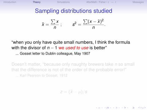
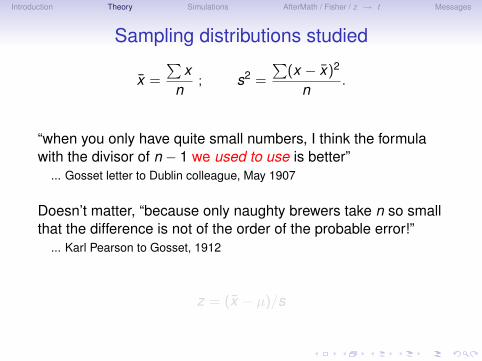
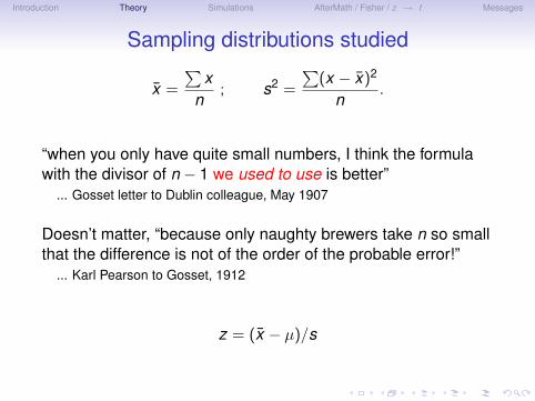
Sampling distributions studied
x̄ =
∑x
n; s2 =
∑(x − x̄)2
n.
“when you only have quite small numbers, I think the formulawith the divisor of n − 1 we used to use is better”
... Gosset letter to Dublin colleague, May 1907
Doesn’t matter, “because only naughty brewers take n so smallthat the difference is not of the order of the probable error!”
... Karl Pearson to Gosset, 1912
z = (x̄ − µ)/s
Introduction Theory Simulations AfterMath / Fisher / z → t Messages
Sampling distributions studied
x̄ =
∑x
n; s2 =
∑(x − x̄)2
n.
“when you only have quite small numbers, I think the formulawith the divisor of n − 1 we used to use is better”
... Gosset letter to Dublin colleague, May 1907
Doesn’t matter, “because only naughty brewers take n so smallthat the difference is not of the order of the probable error!”
... Karl Pearson to Gosset, 1912
z = (x̄ − µ)/s

Introduction Theory Simulations AfterMath / Fisher / z → t Messages
Three steps to the distribution of z
Section I
• Derived first 4 moments of s2.• Found they matched those from curve of Pearson’s type III.• “it is probable that that curve found represents the
theoretical distribution of s2.” Thus, “although we have noactual proof, we shall assume it to do so in what follows.”
Section II• “No kind of correlation” between x̄ and s• His proof is incomplete: see ARTICLE in The American Statistician.

Introduction Theory Simulations AfterMath / Fisher / z → t Messages
Section III• Derives the pdf of z:
• joint distribution of {x̄ , s}• transforms to that of {z, s},• integrates over s to obtain pdf (z) ∝ (1 + z2)−n/2.
Sections IV and V• ..• ..

Introduction Theory Simulations AfterMath / Fisher / z → t Messages
Section III• Derives the pdf of z:
• joint distribution of {x̄ , s}• transforms to that of {z, s},• integrates over s to obtain pdf (z) ∝ (1 + z2)−n/2.
Sections IV and V• ..• ..

Introduction Theory Simulations AfterMath / Fisher / z → t Messages
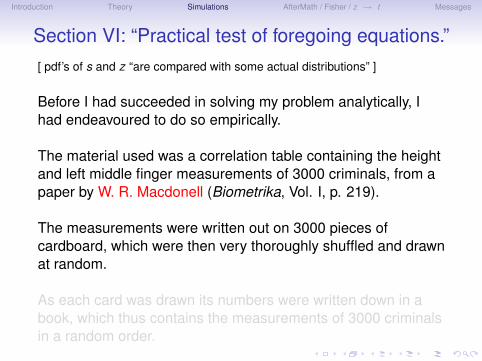
Section VI: “Practical test of foregoing equations.”[ pdf’s of s and z “are compared with some actual distributions” ]
Before I had succeeded in solving my problem analytically, Ihad endeavoured to do so empirically.
The material used was a correlation table containing the heightand left middle finger measurements of 3000 criminals, from apaper by W. R. Macdonell (Biometrika, Vol. I, p. 219).
The measurements were written out on 3000 pieces ofcardboard, which were then very thoroughly shuffled and drawnat random.
As each card was drawn its numbers were written down in abook, which thus contains the measurements of 3000 criminalsin a random order.

Introduction Theory Simulations AfterMath / Fisher / z → t Messages
Section VI: “Practical test of foregoing equations.”[ pdf’s of s and z “are compared with some actual distributions” ]
Before I had succeeded in solving my problem analytically, Ihad endeavoured to do so empirically.
The material used was a correlation table containing the heightand left middle finger measurements of 3000 criminals, from apaper by W. R. Macdonell (Biometrika, Vol. I, p. 219).
The measurements were written out on 3000 pieces ofcardboard, which were then very thoroughly shuffled and drawnat random.
As each card was drawn its numbers were written down in abook, which thus contains the measurements of 3000 criminalsin a random order.

Introduction Theory Simulations AfterMath / Fisher / z → t Messages
continued ...
Finally, each consecutive set of 4 was taken as a sample – 750in all – and the mean, standard deviation, and correlation ofeach sample determined.
The difference between the mean of each sample and themean of the population was then divided by the standarddeviation of the sample, giving us the z of Section III.
This provides us with two sets of 750 standard deviations andtwo sets of 750 z ’s on which to test the theoretical resultsarrived at.

Introduction Theory Simulations AfterMath / Fisher / z → t Messages
Inside cover of one of Gosset’s notebooks...
photo courtesy of Elizabeth Turner LSHTM, and UCL archives.

Introduction Theory Simulations AfterMath / Fisher / z → t Messages
Macdonell’s data
See HANDOUT & WEBSITE

Introduction Theory Simulations AfterMath / Fisher / z → t Messages
Our simulations, 100 years later
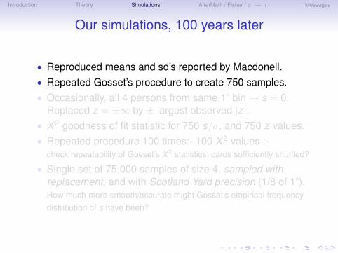
• Reproduced means and sd’s reported by Macdonell.• Repeated Gosset’s procedure to create 750 samples.• Occasionally, all 4 persons from same 1” bin→ s = 0.
Replaced z = ±∞ by ± largest observed |z|.• X 2 goodness of fit statistic for 750 s/σ, and 750 z values.• Repeated procedure 100 times:- 100 X 2 values :-
check repeatability of Gosset’s X 2 statistics; cards sufficiently shuffled?
• Single set of 75,000 samples of size 4, sampled withreplacement, and with Scotland Yard precision (1/8 of 1”).How much more smooth/accurate might Gosset’s empirical frequencydistribution of s have been?

Introduction Theory Simulations AfterMath / Fisher / z → t Messages
Our simulations, 100 years later
• Reproduced means and sd’s reported by Macdonell.• Repeated Gosset’s procedure to create 750 samples.• Occasionally, all 4 persons from same 1” bin→ s = 0.
Replaced z = ±∞ by ± largest observed |z|.• X 2 goodness of fit statistic for 750 s/σ, and 750 z values.• Repeated procedure 100 times:- 100 X 2 values :-
check repeatability of Gosset’s X 2 statistics; cards sufficiently shuffled?
• Single set of 75,000 samples of size 4, sampled withreplacement, and with Scotland Yard precision (1/8 of 1”).How much more smooth/accurate might Gosset’s empirical frequencydistribution of s have been?

Introduction Theory Simulations AfterMath / Fisher / z → t Messages
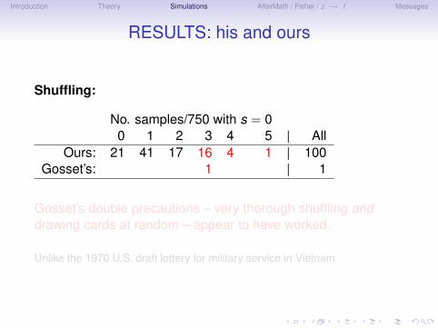
RESULTS: his and ours
Shuffling:
No. samples/750 with s = 00 1 2 3 4 5 | All
Ours: 21 41 17 16 4 1 | 100Gosset’s: 1 | 1
Gosset’s double precautions – very thorough shuffling anddrawing cards at random – appear to have worked.
Unlike the 1970 U.S. draft lottery for military service in Vietnam
Introduction Theory Simulations AfterMath / Fisher / z → t Messages
RESULTS: his and ours
Shuffling:
No. samples/750 with s = 00 1 2 3 4 5 | All
Ours: 21 41 17 16 4 1 | 100Gosset’s: 1 | 1
Gosset’s double precautions – very thorough shuffling anddrawing cards at random – appear to have worked.
Unlike the 1970 U.S. draft lottery for military service in Vietnam

Introduction Theory Simulations AfterMath / Fisher / z → t Messages
Distribution of s/σ
0.0 0.5 1.0 1.5 2.0 2.5
020
0040
0060
0080
0010
000
Scale of standard deviation
Freq
uenc
y
ExpectedObserved (75000 samples)!2 = 63.1P < 0.0001Observed (750 samples)!2 = 42.4P = 0.0006
Summary of !2values
for 100 simulationsMean: 53.2Median: 51.4Minimum: 29.8Maximum: 98.0Standard deviation: 13.8
Dotted line: Samplestatistics obtained fromone set of 750 randomsamples generated byGosset’s procedure.Inset: distr’n of 100 X 2
statistics (18 intervals).Thin solid line: distr’n ofstatistics obtained from75,000 samples of size 4sampled with replacementfrom 3000 heightsrecorded to nearest 1/8”.

Introduction Theory Simulations AfterMath / Fisher / z → t Messages
Distribution of z
!4 !2 0 2 4
010
0020
0030
0040
0050
00
Scale of z
Freq
uenc
y
ExpectedObserved (75000 samples)!2 = 16.9P = 0.3
Observed (750 samples)!2 = 17.2P = 0.3
Summary of !2valuesfor 100 simulations
Mean: 16.9Median: 16.9Minimum: 4.6Maximum: 33.4Standard deviation: 6.3
Dotted line: Samplestatistics obtained fromone set of 750 randomsamples generated byGosset’s procedure.Inset: distribution of 100X 2 statistics (15 intervals).Thin solid line: distr’n ofstatistics obtained from75,000 samples of size 4sampled with replacementfrom 3000 heightsrecorded to nearest 1/8”.

Introduction Theory Simulations AfterMath / Fisher / z → t Messages
If Gosset had R :
“Agreement between observed and expected frequencies of the750 s/σ’s was not good”. He attributed this to coarse scale of s.
Distribution of our 75,000 s/σ values also shows pattern oflarge deviations similar to those in table on p. 15 of his paper.
Scotland Yard precision and today’s computing power wouldhave left Gosset in no doubt that the distribution of s which he“assumed” was correct was in fact correct.
Grouping had not had so much effect on distr’n of z ’s: “closecorrespondence between the theory and the actual result.”

Introduction Theory Simulations AfterMath / Fisher / z → t Messages
FOR...
• Description of remainder of 1908 article• Early extra-mural use of Gosset’s distribution• Fisher’s geometric vision• Fisher and Gosset , and transition z → t
SEE..
• SLIDES FROM LONGER VERSION OF TALK• ARTICLE in The American Statistician• http://www.epi.mcgill.ca/hanley/Student

Introduction Theory Simulations AfterMath / Fisher / z → t Messages
Triumphator A ser 43219
http://www.calculators.szrek.com/

Introduction Theory Simulations AfterMath / Fisher / z → t Messages
Millionaire Ser 1200

Introduction Theory Simulations AfterMath / Fisher / z → t Messages
To students of statistics in 2008 ... (I)
Fisher1939:• “of (Gosset’s) personal characteristics, the most obvious
were a clear head, and a practice of forming independentjudgements.”
• The other was the importance of his work environment:“one immense advantage that Gosset possessed was theconcern with, and responsibility for, the practicalinterpretation of experimental data.”
Gosset stayed very close to these data.
We should too!

Introduction Theory Simulations AfterMath / Fisher / z → t Messages
To students of statistics in 2008 ... (II)
Compared with what Gosset could do, today we can run muchmore extensive simulations to test our new methods.
Which pseudo-random observations are more appropriate:those from perfectly behaved theoretical populations, or thosefrom real datasets, such as Macdonell’s?
In light of how Gosset included the 3 infinite z-ratios, we mightre-examine how we deal with problematic results in our runs.

Introduction Theory Simulations AfterMath / Fisher / z → t Messages
To students of statistics in 2008 ... (III)
The quality of writing – and statistical writing – is declining.
Today’s students – and teachers – would do well to heed E.S.Pearson’s 1939 advice regarding writing and communication.
E.S. Pearson on Gosset’s ‘P.E. of Mean’ paper...
“It is a paper to which I think all research students in statisticsmight well be directed, particularly before they attempt to puttogether their own first paper."
JH ...
Read work of Galton, Karl Pearson, Gosset, E.S. Pearson,Cochran, Mosteller, David Cox, Stigler, ... for content and style.

Introduction Theory Simulations AfterMath / Fisher / z → t Messages
To students of statistics in 2008 ... (IV)
When JH was a student, very little of the historical material wehave reviewed here was readily available.
Today, we are able to obtain it, review it, and follow up leads –all from our desktops – via Google, and using JSTOR and otheronline collections.
Statistical history need no longer be just for those who grew upin the years “B.C.”
Become Students of the History of Statistics
“B.C.”: Before Computers.

Introduction Theory Simulations AfterMath / Fisher / z → t Messages
FUNDING / CO-ORDINATES
Natural Sciences and Engineering Research Council of Canada
http://www.biostat.mcgill.ca/hanley
BIOSTATISTICS
http:/p: /wwwwwww.mw.mw.mmcgill.ca/ca/a epiepiepiepi-bibbiostosts at-at-aa occh/g/ggrad/bib ostatistit cs/