student laboratory manuals - uzhmatthias/espace-assistant/manuals/en/anleitung... · second...

Teil I

Student Laboratory Manuals

1

5. Fluid friction in liquids

IR1

5.1 Introduction

Generally the term fluid is understood to be matter either in the gaseous or liquid state. The physicsinvolved on the macroscopic scale is essentially the same; the difference is orders of magnitude indensity and therefore molecular distance and the corresponding forces acting. The experimentaltechniques required for investigating gases or liquid are quite different, though. In this text fluidrefers to the liquid state, if not otherwise explicitly stated.

A fluid flows, e.g. in a tube, not as solid ’plug’, but with more or less complicated internal motionwith continuously changing velocities at all points of reference in the fluid. Resistance to flow stemsfrom attractive forces between the molecules, and therefore work is required if molecules are to beseparated, as in a flowing liquid. For the many molecules in a macroscopic fluid sample, it wouldbe impractical to try to calculate this work on the molecular level. Instead, at least for engineeringpurposes, a different approach is adopted. As is often the case when the underlying physics is toocomplicated for direct access, or the effort would not be rewarding, a phenomenological view isapplied, and the physical mechanisms described by using easily measured macroscopic materialparameters. One such case is friction of any kind, and in particular the internal forces that makea fluid resist motion : the observed phenomenon is reduced to a parameter that we will examinebelow: viscosity ; the collective resistance to motion by the molecular forces is referred to as fluidfriction.

Returning briefly to the molecular level, we recall that polyatomic molecules are stabilized byinternal, or intramolecular forces between atoms or groups of atoms, which are not of concern here,whilst fluid friction is determined by the forces between the molecules, the intermolecular forces.

We also note that the intermolecular forces are attractive, but in a fluid rather weak. The weakbinding between molecules may typically be described as Van der Waals forces or hydrogen bonds,the latter, e.g. for the important case of water and watery solutions.

Practical and economical consequences of engineering design are found in all kind of installationsinvolving extensive tubing, as is the case for heat exchangers, thermal (steam) power stations,nuclear power reactors, hydropower stations, oil refineries, chemical processing plants, paper mills,but also on a different scale, the system of human blood vessels; In all these cases careful designwas employed to balance tubing diameter and viscosity against desired flow characteristics.

In this laboratory we investigate fluid friction in two important cases: the flow resistance of liquids

3

4 5. Fluid friction in liquids

FR

Fυ

d υ

Abbildung 5.1: Principle of measuring the Newtonian fluid friction.

in capillary tubes, and its dependence on tube diameter, for water and castor oil (ricinus); In asecond experiment, the resistance to motion of spherical balls falling by gravity, again in water andcastor oil.

Both methods are developed for quantitative determination of fluid friction, and determine quan-titatively the coefficient of viscosity

In particular we also introduce the Reynolds number as an important characteristic of fluid flow.

5.2 Theory

a) Newtons law for Fluids – Newtonian fluids

A Newtonian fluid (named so for Isaac Newton) is a fluid whose stress versus strain rate curve islinear and passes through the origin. The constant of proportionality is known as the viscosity ofthe fluid1.

In common terms, this means that the fluid continues to flow, regardless of the forces acting on it.For example, water is Newtonian, because it continues to show fluid properties no matter how fastit is stirred or mixed. In contrast, a non-Newtonian fluid changes its properties: stirring can leavea ’hole’ behind because the fluid becomes thicker (Rheopecty; this behaviour is seen in materialssuch as pudding, starch in water). The non-Newtonian fluid may also become thinner with stirring,the drop in viscosity causing it to flow better (Thixotropy; this property has been put to gooduse in non-drip paints, which easily wet the brush because they flow easily, but become moreviscous(thicker) when applied by brushstroke on a wall).

Next we need to define two common notions used to describe fluid motion: laminar flow sometimesknown as streamline flow, occurs when a fluid flows in parallel layers. The appearance is smooth.

Flow that is not laminar is termed turbulent. It is characterised by whirls, or in more technicallanguage by eddies and vortices and generally by chaotic, property changes. There is rapid variationof pressure and velocity in space and time. The appearance is rough.

Extended piping systems, as used for district heating or chemical industry, need to be designed for

1The material properties stress, strain and shear are introduced in laboratory TB.

Laboratory Manuals for Physics Majors - Course PHY112/122

5.2. THEORY 5

laminar flow since this requires the least pumping power and causes less vibrations and materialdetoriation. For applications where heat exchangers and reaction vessels are involved, turbulentflow is essential for good heat transfer and mixing, since in this flow regime there is flow alsotransversely to the general flow direction.

Employing a simple model for laminar flow, we may assume infinitely thin parallel fluid sheets movewith different velocities such that frictional forces ~FR between the sheets act to set up shear stress.We also characterise ~FR as drag. This model is depicted in Fig. 5.1 : A layer of fluid is enclosedbetween two plates. If this frictional force causes the substance between the plates to undergo shearflow (as opposed to just elastic shearing, as for a solid, until the shear stress balances the appliedforce), the substance is called a fluid.

We assume here that the lower plate is stationary, and that the upper moves with a relative velocityv. It is further assumed that the attraction between the plates and the fluid is such that next toeach plate there is a fluid sheet that does not move relative to the plate. As a consequence thevelocities for each sheet changes with distance, as shown in the figure. In particular we note alreadyhere, that in the figure the change in velocity is linear with distance between the plate. This is nottrivial, and we return to this subject later. The principle shown may be directly implemented inan apparatus for measuring fluid resistance, for instance by using two parallel rotating plates.

Under steady state conditions, an external force F = FR is required to maintain the velocity v ofthe upper plate. For velocities not too high, and a plate distance d small compared to the area Aof the upper plate (in order to avoid edge effects), the force F = FR is proportional to the area andvelocity v of the upper plate and inversely proportional to the distance:

FR = η ·A · vd

(5.1)

Here η is a property variable characterising the thicknessor ßtiffnessof the liquid. Written is thisform the relation is valid only for the chosen geometry of parallel plates; for the same liquid flowing,e.g. in a tube, the ratio v/d, the rate of shear deformation, varies with distance.

For straight, parallel and uniform flow, as in this case, it was postulated by Newton, that the shearstress, τ , between layers is proportional to the velocity gradient in the direction perpendicular tothe fluid sheets. This is the Newton’s criterion, and may taken as a definition of a Newtonian fluid.The relation Eq. 5.1 then may be written on the equivalent but more general form:

τ ≡ FR(z)A

= η · dvdz

(5.2)

The factor of proportionality is by definition the viscosity, here designated η. Many fluids, suchas water and most gases, satisfy Newton’s criterion, that their flow be described by Eq. 5.2. Bydefinition, the viscosity depends only on temperature and pressure, but not on the forces actingupon it.

It is worth noting, that it is the strength of the velocity gradient dvdz perpendicular to the flow

direction that determines the drag, the resistance to flow. In our intuitive picture of laminar flow,this is because of the friction in the fluid sheets gliding past each other. In practice this property



determines the time for a certain fluid to flow through a given tube, or the pumping power requiredfor a certain volume throughput.

The coefficient of viscosity η, as defined through the relations Eq. 5.1 and Eq. 5.2, is the mostcommon variant, and is therefore often called just viscosity or absolute viscosity. More specificnames are the dynamic viscosity, or the Newtonian viscosity. The reader is advised, that severaldifferently defined coefficient of viscosity are found in the literature (see below).

Non-Newtonian fluids exhibit a more complex relationship between shear stress and velocity gra-dient than simple linearity as in Eq. 5.2. Examples include polymer solutions, molten polymers,blood ketchup, shampoo, suspensions of starch2, many solid suspensions and most highly viscousfluids. It is not the ’thickness’ per se that makes a fluid non-Newtonian, but the complicated in-teraction between large molecules or chains of molecules. As already mention above, an indicationdemonstrating the nonlinearity, is the drop in viscosity seen when stirring non-drip paints,

The viscosity is a strongly temperature dependent parameter, as we know already from everydayexperience.

Some common viscosity coefficients

Several different viscosity coefficients are in use, depending on the method for applying stress andthe nature of the fluid, i.e. the type of application targeted. Specialised methods of measurement,and corresponding units are in use for industrial applications, in particular petrochemical. ForNewtonian fluids, dynamic viscosity and kinematic viscosity are common, and often confused. Ifin doubt, always note the unit. We list some of the most common coefficients for the sake ofcompleteness here:

Viscosity coefficients for Newtonian fluids

• Dynamic viscosity (introduced above) determines the dynamics of an incompressible Newto-nian fluid.

• Kinematic viscosity is the dynamic viscosity divided by the density for a Newtonian fluid.

• Volume viscosity (or bulk viscosity) determines the dynamics of a compressible Newtonianfluid.

Viscosity coefficients for non-Newtonian fluids

• Shear viscosity is the viscosity coefficient when the applied stress is a shear stress (valid fornon-Newtonian fluids).

• Extensional viscosity is the viscosity coefficient when the applied stress is an extensional stress(valid for non-Newtonian fluids; widely used for characterising polymers).

2Those of the readers having been exposed to a British education may be familiar with the substance oobleck,

which gets its name from the Dr. Seuss book Bartholomew and the Oobleck, where a gooey green substance, oobleck,

fell from the sky and wreaked havoc in the kingdom.


5.2. THEORY 7

Shear viscosity and dynamic viscosity are the best known in each of the two groups: both defined asthe ratio between the pressure exerted on the surface of a fluid, in the lateral or horizontal direction,to the change in velocity of the fluid as you move down in the fluid (this is what is referred to as avelocity gradient).

Units and nomenclature

Dynamic viscosity: The symbol commonly used for dynamic viscosity by mechanical and chemicalengineers is µ, whereas η is commonly preferred by chemists and IUPAC3.

The SI unit of dynamic viscosity is the pascal-second (Pa·s), which in SI base units is expressedas kg·m−1·s−1. If a fluid with a viscosity of one Pas is put between two plates, and one plateis displaced horizontally, creating a shear stress of one pascal, it moves a distance equal to thethickness of the layer between the plates in one second.

The cgs physical unit for dynamic viscosity is the poise (P)4. It is more commonly expressed,particularly in ASTM5 standards, as centipoise (cP). Water at 20 oC has a viscosity of 1.0020 cP.1 P = 1 g·cm−1·s−1. The relation between poise and pascal-seconds is: 10 P = 1 kg·m−1·s−1 = 1Pa·s, 1 cP = 0.001 Pa·s = 1 mPa·s. The name ’poiseuille’ (Pl) has been proposed for this unit, alsoafter Jean Louis Marie Poiseuille but has not been accepted internationally. Care must be taken innot confusing these units where they might appear.

Kinematic viscosity: In many situations we are concerned with the ratio of the viscous force to theinertial force per unit volume, ρ · g. For this purpose the kinematic viscosity ν is defined as:

ν =η

ρ(5.3)

where, as before, η is the dynamic viscosity [Pas], ρ is the mass density [kg·m−3], and ν is thekinematic viscosity [m2s−1]. The cgs unit for kinematic viscosity is the stokes (St), named afterGeorge Gabriel Stokes. It is sometimes expressed in terms of centistokes (cSt or ctsk). 1 stokes= 100 centistokes = 1 cm2s−1 = 0.0001 m−2·s−1. 1 centistokes = 1 mm2·s−1 = 10−6m2·s−1. Thekinematic viscosity is sometimes referred to as diffusivity of momentum, because it is comparableto, and has the same SI-dimension [m2s−1] as diffusivity of heat and diffusivity of mass. It is usedin dimensionless numbers for the comparison of the ratio of the diffusivities.

1 Poise = 1g

cm · s= 0.1 Pa · s (5.4)

3The International Union for Pure and Applied Chemistry4named after Jean Louis Marie Poiseuille, who formulated Poiseuille’s law of viscous flow.5ASTM International (ASTM), originally known as the American Society for Testing and Materials, is an interna-

tional standards organisation that develops and publishes voluntary consensus technical standards for a wide range

of materials, products, systems, and services.



b) The Hagen-Poiseuille Equation

Using Newton’s law of fluids, as discussed above, we now develop an expression for laminar flow ina cylindrical tube of length l and inner radius R (cf Fig. 5.2).

For the analysis we choose a concentric cylindrical volume element of fluid of radius r ≤ R. Becauseof a pressure difference ∆p = p1 − p2 persisting between the ends of the tube, a net force Fp actson the cylindrical element:

Fp = π · r2 ·∆p (5.5)

According to Eq. 5.2, the velocity gradient perpendicular to the cylinder axis (dv/dr)|r gives riseto a drag force FR at the distance r from the axis:

FR = η · 2π · r · l ·(dv

dr

)∣∣∣∣r

(5.6)

For stationary conditions (no change in the velocity profile with time), a balance between thepressure induced force FP and the frictional drag FR persists, which we write as:

π · r2 ·∆p+ η · 2π · r · l ·(dv

dr

)∣∣∣∣r

= 0 (5.7)

From this we may express the velocity gradient at distance r from the cylinder axis

(dv

dr

)∣∣∣∣r

= − ∆p2 η · l

· r (5.8)

The actual flow speed v(r) may be obtained by solving this differential equation, which because ofthe simple form amounts to an integration using the given boundary condition v(r = R) = 0:

v(r) =∆p

4 η · l· (R2 − r2) (5.9)

This is a parabolic velocity distribution as shown in Fig. 5.3. The maximum velocity is found atr = 0 in the centre of the tube, from where it decreases quadratically with increasing r, becomingzero at the wall of the tube.

p1

FR FP

p2

Rr

l

Abbildung 5.2: Forces and pressures acting on a fluid in a section of a cylindrical tube.


5.2. THEORY 9

r

υmax

υ(r)

Abbildung 5.3: Velocity profile in a cylindrical tube.

Using the geometry of Fig. 5.4, the amount dQ of fluid flowing through an annular cylinder ofradius r in time t,) may be expressed as:

dQ = t · v(r) · 2π · r · dr = t · π · r ·∆p · (R2 − r2)

2 η · ldr (5.10)

Integrating this equation over the cross section of the tube we arrive at the Hagen-Poiseuille Equa-tion for for the amount Q flowing in tie t:

Q = t ·∫ R

0

π · r ·∆p · (R2 − r2)2 η · l

dr =π ·R4 ·∆p

8 η · l· t (5.11)

The reader is urged to perform a dimensional analysis of this expression in order to determine thecorrect unit of Q.

If the dimensions of the tube is known, the viscosity η of the fluid given may be determined frommeasured values of Q, t and ∆p.

c) Laminar and turbulent flow – Reynolds number.

Newtons equation 5.2 is valid only for the case of laminar flow, as discussed above. For flow that isfaster than a certain critical value vkrit the laminar flow lines are disturbed by an unruly behaviourand may develop vortex patterns that depends on the given geometry. This is the regime of turbulentflow that is characterised by fluid motion also transversely to the direction of flow. The complicatedflow pattern of turbulent flow requires more power for the same volume throughput, which isequivalent to a higher flow resistance. For a given system of fluid and geometry, it is found thatthe critical velocity vkrit is determined by the mass density ρ the viscosity η and a characteristicdimension d of the system (e.g. the diameter of the tube in case of a cylindrical tube). In thestudy of macroscopic phenomenology of physics and engineering, surprisingly simple dimensionlesscombinations of measurable entities have proved themselves to faithfully characterise otherwisehighly complicated systems.

dr

r

Abbildung 5.4: Geometry for the development of Hagen-Poiseuille Equation.



As a characteristic of fluid flow, the dimensionless number defined as

Re =ρ · v · dη

(5.12)

has emerged through measurement and intuition. This is Reynold’s number, and it turns out thatbelow a certain value Rekrit laminar flow is present, whereas for Re > Rekrit turbulent flow prevails.

For straight, cylindrical tubes Rekrit ≈ 2300. Eq. 5.12 the gives us:

vkrit = 2300η

ρ · d(5.13)

where d is the diameter of the tube. The flow remains laminar as long as the mean flow velocityis below vkrit . The remarkable feature of Reynold’s number, or any other of several dimensionlessnumber, is that any combination of the values of the measurable properties, consistently describeproperties of the materal.

d) Stoke’s equation

For highly viscous fluids (high η), such as oil at low temperatures, the throughput in a capillarywould be so slow that the viscosity η could not practically be determined. In such cases an effectiveand simple alternative method is to measure the time of fall by gravity of a sphere in the fluidof interest. The forces acting on the sphere is shown in Fig. 5.5. The force of gravity FG and thebouyancy FA are respectively:

FG = m · g =43π · r3ρK · g

FA =43π · r3 · ρFl · g

where ρK is the mass density and r the radius of the sphere and ρFl the density of the fluid.

For the drag force FR, we have for laminar flow the frictional law of Stoke:

FR = 6π · η · r · v (5.14)

FA

FG

FR

z

Abbildung 5.5: Forces acting on a sphere falling through a viscous fluid.


5.2. THEORY 11

where

η = viscosity of the fluid

r = radius of the fluid

v = terminal velocity of the sphere

The frictional force FR is proportional to the velocity and thus for some velocity, the terminalvelocity, a stationary condition is reached with constant velocity (see appendix). The forces actingon the sphere balances each other according to the relation:

43π · r3 · (ρK − ρFl ) · g − 6π · η · r · v = 0 (5.15)

If the mass density ρ and the radius of sphere R are known, the viscosity η may be determinedfrom a measured value of the terminal velocity.

η =2 r2 · g · (ρK − ρFl )

9 v(5.16)



5.3 Experimental

a) Determination of the viscosity of water

The viscosity of water is determined according to Eq. 5.11. The amount of water Q collected from acapillary of radius R and length l in time ∆t is determined6?. The measurement is made using threedifferent capillaries (five are provided, marked with roman numerals I - V). Check which capillariesthat work – the two smallest diameters probably does not allow laminar flow, and should thereforenot be used (recall that the equations developed are valid only for laminar flow). Make sure thatde-mineralized (or destilled) water is used in the experiment, since otherwise deposits are left inthe capillaries (de-mineralized water may be found in rooms 11 G 24 and 11 G 26: water taps withgreen rings and text). With most capillaries there is some dripping at the same time as the waterflows nicely. It is left to the discretion of the experimentalist to handle this matter in a reasonableway.

The experimental set-up is shown in Fig. 5.6. A vertical glass cylinder with volume markings hasa provision for mounting the capillaries at the output in the lower part of the cylinder. For givenheight h of the fluid column, the pressure difference ∆p = p1−p2 between the ends of the capillarieswill be:

∆p = p1 − p2 = pL + ρ · g · h− pL = ρ · g · h (5.17)

• Measure the length l of the capillaries. The inner diameter is given at the lab desk. Mountone of the capillaries at the outlet of the cylinder.

• Fill the cylinder with de-mineralised water. For each of the different capillaries there mightbe a highest level above which the flow through the capillary will not be laminar. This hasto be tested. The same might be true for a lowest level.

6Make certain that you know the meaning of Q: what is the SI-unit in 5.11

atmospheric pressure

pL

pL

ρW

h

l

2r

Abbildung 5.6: Set-up for determining the viscosity of water.


5.3. EXPERIMENTAL 13

• Let the water running from the capillary collect in a cup during the time interval t, for knownheights ha and hb. The time should not be too short, since then errors might become large.

• Determine the amount of water Q using the electronic scale, and correct for the mass of theempty cup.

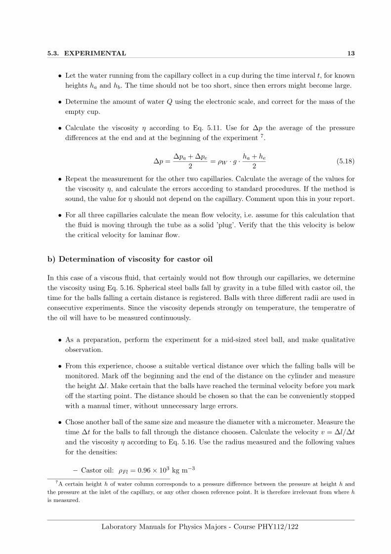
• Calculate the viscosity η according to Eq. 5.11. Use for ∆p the average of the pressuredifferences at the end and at the beginning of the experiment 7.

∆p =∆pa + ∆pe

2= ρW · g ·

ha + he

2(5.18)

• Repeat the measurement for the other two capillaries. Calculate the average of the values forthe viscosity η, and calculate the errors according to standard procedures. If the method issound, the value for η should not depend on the capillary. Comment upon this in your report.

• For all three capillaries calculate the mean flow velocity, i.e. assume for this calculation thatthe fluid is moving through the tube as a solid ’plug’. Verify that the this velocity is belowthe critical velocity for laminar flow.

b) Determination of viscosity for castor oil

In this case of a viscous fluid, that certainly would not flow through our capillaries, we determinethe viscosity using Eq. 5.16. Spherical steel balls fall by gravity in a tube filled with castor oil, thetime for the balls falling a certain distance is registered. Balls with three different radii are used inconsecutive experiments. Since the viscosity depends strongly on temperature, the temperatre ofthe oil will have to be measured continuously.

• As a preparation, perform the experiment for a mid-sized steel ball, and make qualitativeobservation.

• From this experience, choose a suitable vertical distance over which the falling balls will bemonitored. Mark off the beginning and the end of the distance on the cylinder and measurethe height ∆l. Make certain that the balls have reached the terminal velocity before you markoff the starting point. The distance should be chosen so that the can be conveniently stoppedwith a manual timer, without unnecessary large errors.

• Chose another ball of the same size and measure the diameter with a micrometer. Measure thetime ∆t for the balls to fall through the distance choosen. Calculate the velocity v = ∆l/∆tand the viscosity η according to Eq. 5.16. Use the radius measured and the following valuesfor the densities:

– Castor oil: ρFl = 0.96× 103 kg m−3

7A certain height h of water column corresponds to a pressure difference between the pressure at height h and

the pressure at the inlet of the capillary, or any other chosen reference point. It is therefore irrelevant from where h

is measured.



– Steel ball: ρK = 7.86× 103 kg m−3

• Repeat the measurement for five different mid-sized balls, and then for five different balls oflarger, and five different of smaller size. If necessary, chose different height distances for ballsof different size.

• Determine the average of the results and calculate the errors appropriately.


5.4. APPENDIX 15

5.4 Appendix

The equation of motion for the falling ball (Newton’s law of motion) is developed from the genericform:

F = m · a (5.19)

For the acceleration we write:

a ≡ d2

dt2≡ dv

dt(5.20)

With notation and reference direction as in Fig. 5.5, the external forces acting are:

F = FG − FA − FR (5.21)

In particular we know that FR = 6π · η · r · v, which we for simplicity write as FR = β · v. For thesame reason we write α = FG − FA, from which we then have the equation of motion as a firstorder ordinary differential equation (ODE) in v = dz/dt:

m · dvdt

= α− β · v (5.22)

Note, that α is always zero, if we may assume that the density of the ball is greater that that ofthe fluid. The solution to the differential equation could be easily found with conventional methods(it is an exponential determined by the boundary conditions), we chose here to discuss the relationphenomenologically. Although we are interested only in the stationary solution, we start with ageneral approach to this equation.

Positive reference direction is in the direction of gravitation. Assuming that the initial speed of theball is zero, then, since α > 0, the left side of the equation also have to be positive, i.e. dv/dt > 0meaning that the speed increases (in a more direct view of matters, this has to be the case since theball falls by gravity because of the higher density of the ball) Since α is independent of the velocity,and the term β · v now increases, but has a negative sign, the right side of the ODE will decrease,requiring the derivative on the left side to become smaller. Eventually a stationary condition isreached as the ball attains its (constant) terminal velocity.

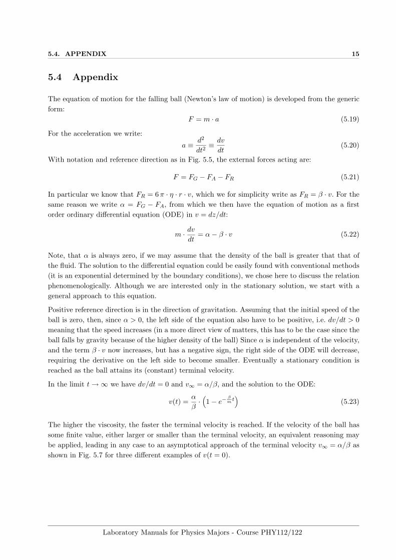
In the limit t→∞ we have dv/dt = 0 and v∞ = α/β, and the solution to the ODE:

v(t) =α

β·(1− e−

βm

t)

(5.23)

The higher the viscosity, the faster the terminal velocity is reached. If the velocity of the ball hassome finite value, either larger or smaller than the terminal velocity, an equivalent reasoning maybe applied, leading in any case to an asymptotical approach of the terminal velocity v∞ = α/β asshown in Fig. 5.7 for three different examples of v(t = 0).



υ

υ0

υ∞

t0

υ0

Abbildung 5.7: Change of velocity for a ball falling in a viscous fluid for three different initialvelocities: v(t = 0) = 0 (solid linie) and two different v(t = 0) > 0 (broken lines).


student laboratory manuals - uzhmatthias/espace-assistant/manuals/en/anleitung... · second...

Documents