stt 455-6: actuarial models - michigan state...
TRANSCRIPT

STT 455-6: Actuarial Models
Albert Cohen
Actuarial Sciences ProgramDepartment of Mathematics
Department of Statistics and ProbabilityA336 Wells Hall
Michigan State UniversityEast Lansing MI
[email protected]@stt.msu.edu
Albert Cohen (MSU) STT 455-6: Actuarial Models MSU 2011-12 1 / 283

Copyright Acknowledgement
Many examples and theorem proofs in these slides, and on in class exampreparation slides, are taken from our textbook ”Actuarial Mathematics forLife Contingent Risks” by Dickson,Hardy, and Waters.
Please note that Cambridge owns the copyright for that material.No portion of the Cambridge textbook material may be reproducedin any part or by any means without the permission of thepublisher. We are very thankful to the publisher for allowing postingof these notes on our class website.
Also, we will from time-to-time look at problems from releasedprevious Exams MLC by the SOA. All such questions belong incopyright to the Society of Actuaries, and we make no claim onthem. It is of course an honor to be able to present analysis of suchexamples here.
Albert Cohen (MSU) STT 455-6: Actuarial Models MSU 2011-12 2 / 283
Survival Models
An insurance policy is a contract where the policyholder pays apremium to the insurer in return for a benefit or payment later.
The contract specifies what event the payment is contingent on. Thisevent may be random in nature
Assume that interest rates are deterministic, for now
Consider the case where an insurance company provides a benefitupon death of the policyholder. This time is unknown, and so theissuer requires, at least, a model of of human mortality
Albert Cohen (MSU) STT 455-6: Actuarial Models MSU 2011-12 3 / 283
Survival Models
Define (x) as a human at age x . Also, define that person’s future lifetimeas the continuous random variable Tx . This means that x + Tx representsthat person’s age at death.
Define the lifetime distribution
Fx(t) = P[Tx ≤ t] (1)
the probabiliity that (x) does not survive beyond age x + t years, and it’scomplement, the survival function Sx(t) = 1− Fx(t).
Albert Cohen (MSU) STT 455-6: Actuarial Models MSU 2011-12 4 / 283

Conditional Equivalence
We have an important conditional relationship
P[Tx ≤ t] = P[T0 ≤ x + t | T0 > x ]
=P[x < T0 ≤ x + t]
P[T0 > x ]
(2)
and so
Fx(t) =F0(x + t)− F0(x)
1− F0(x)
Sx(t) =S0(x + t)
S0(x)
(3)
In general we can extend this to
Sx(t + u) = Sx(t)Sx+t(u) (4)
Albert Cohen (MSU) STT 455-6: Actuarial Models MSU 2011-12 5 / 283
Conditions and Assumptions
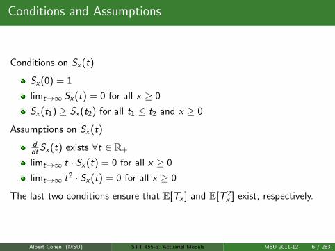
Conditions on Sx(t)
Sx(0) = 1
limt→∞ Sx(t) = 0 for all x ≥ 0
Sx(t1) ≥ Sx(t2) for all t1 ≤ t2 and x ≥ 0
Assumptions on Sx(t)
ddt Sx(t) exists ∀t ∈ R+
limt→∞ t · Sx(t) = 0 for all x ≥ 0
limt→∞ t2 · Sx(t) = 0 for all x ≥ 0
The last two conditions ensure that E[Tx ] and E[T 2x ] exist, respectively.
Albert Cohen (MSU) STT 455-6: Actuarial Models MSU 2011-12 6 / 283

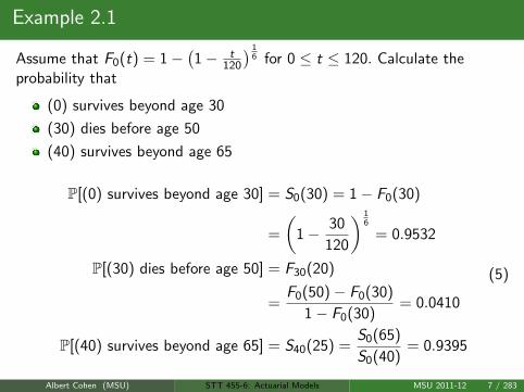
Example 2.1
Assume that F0(t) = 1−(1− t
120
) 16 for 0 ≤ t ≤ 120. Calculate the
probability that
(0) survives beyond age 30
(30) dies before age 50
(40) survives beyond age 65
P[(0) survives beyond age 30] = S0(30) = 1− F0(30)
=
(1− 30
120
) 16
= 0.9532
P[(30) dies before age 50] = F30(20)
=F0(50)− F0(30)
1− F0(30)= 0.0410
P[(40) survives beyond age 65] = S40(25) =S0(65)
S0(40)= 0.9395
(5)
Albert Cohen (MSU) STT 455-6: Actuarial Models MSU 2011-12 7 / 283
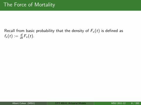
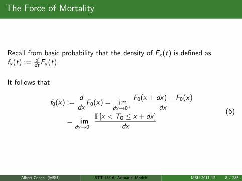
The Force of Mortality
Recall from basic probability that the density of Fx(t) is defined asfx(t) := d
dt Fx(t).
It follows that
f0(x) :=d
dxF0(x) = lim
dx→0+
F0(x + dx)− F0(x)
dx
= limdx→0+
P[x < T0 ≤ x + dx ]
dx
(6)
Albert Cohen (MSU) STT 455-6: Actuarial Models MSU 2011-12 8 / 283
The Force of Mortality
Recall from basic probability that the density of Fx(t) is defined asfx(t) := d
dt Fx(t).
It follows that
f0(x) :=d
dxF0(x) = lim
dx→0+
F0(x + dx)− F0(x)
dx
= limdx→0+
P[x < T0 ≤ x + dx ]
dx
(6)
Albert Cohen (MSU) STT 455-6: Actuarial Models MSU 2011-12 8 / 283
The Force of Mortality
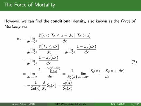
However, we can find the conditional density, also known as the Force ofMortality via
µx = limdx→0+
P[x < T0 ≤ x + dx | T0 > x ]
dx
= limdx→0+
P[Tx ≤ dx ]
dx= lim
dx→0+
1− Sx(dx)
dx
= limdx→0+
1− Sx(dx)
dx
= limdx→0+
1− S0(x+dx)S0(x)
dx=
1
S0(x)lim
dx→0+
S0(x)− S0(x + dx)
dx
= − 1
S0(x)
d
dxS0(x) =
f0(x)
S0(x)
(7)
Albert Cohen (MSU) STT 455-6: Actuarial Models MSU 2011-12 9 / 283
The Force of Mortality
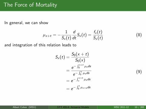
In general, we can show
µx+t = − 1
Sx(t)
d
dtSx(t) =
fx(t)
Sx(t)(8)
and integration of this relation leads to
Sx(t) =S0(x + t)
S0(x)
=e−
∫ x+t0 µsds
e−∫ x
0 µsds
= e−∫ x+tx µsds
= e−∫ t
0 µx+sds
(9)
Albert Cohen (MSU) STT 455-6: Actuarial Models MSU 2011-12 10 / 283
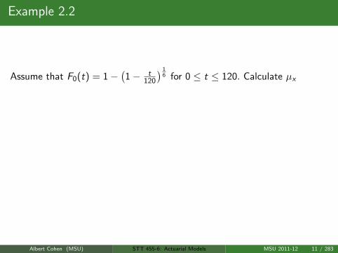
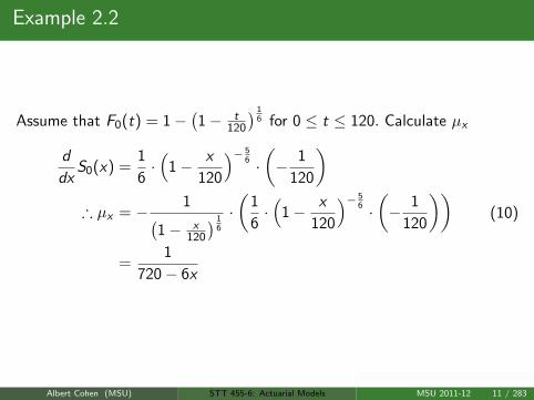
Example 2.2
Assume that F0(t) = 1−(1− t
120
) 16 for 0 ≤ t ≤ 120. Calculate µx
d
dxS0(x) =
1
6·(
1− x
120
)− 56 ·(− 1
120
)∴ µx = − 1(
1− x120
) 16
·(
1
6·(
1− x
120
)− 56 ·(− 1
120
))=
1
720− 6x
(10)
Albert Cohen (MSU) STT 455-6: Actuarial Models MSU 2011-12 11 / 283
Example 2.2
Assume that F0(t) = 1−(1− t
120
) 16 for 0 ≤ t ≤ 120. Calculate µx
d
dxS0(x) =
1
6·(
1− x
120
)− 56 ·(− 1
120
)∴ µx = − 1(
1− x120
) 16
·(
1
6·(
1− x
120
)− 56 ·(− 1
120
))=
1
720− 6x
(10)
Albert Cohen (MSU) STT 455-6: Actuarial Models MSU 2011-12 11 / 283
Gompertz’ Law / Makehams’s Law
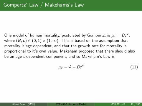
One model of human mortality, postulated by Gompertz, is µx = Bcx ,where (B, c) ∈ (0, 1)× (1,∞). This is based on the assumption thatmortality is age dependent, and that the growth rate for mortality isproportional to it’s own value. Makeham proposed that there should alsobe an age independent component, and so Makeham’s Law is
µx = A + Bcx (11)
Albert Cohen (MSU) STT 455-6: Actuarial Models MSU 2011-12 12 / 283

Gompertz’ Law / Makehams’s Law
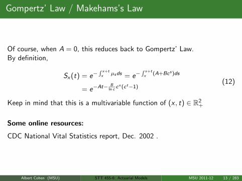
Of course, when A = 0, this reduces back to Gompertz’ Law.
By definition,
Sx(t) = e−∫ x+tx µsds = e−
∫ x+tx (A+Bcs)ds
= e−At−B
ln ccx (ct−1)
(12)
Keep in mind that this is a multivariable function of (x , t) ∈ R2+
Some online resources:
CDC National Vital Statistics report, Dec. 2002 .
Albert Cohen (MSU) STT 455-6: Actuarial Models MSU 2011-12 13 / 283
Gompertz’ Law / Makehams’s Law
Of course, when A = 0, this reduces back to Gompertz’ Law.By definition,
Sx(t) = e−∫ x+tx µsds = e−
∫ x+tx (A+Bcs)ds
= e−At−B
ln ccx (ct−1)
(12)
Keep in mind that this is a multivariable function of (x , t) ∈ R2+
Some online resources:
CDC National Vital Statistics report, Dec. 2002 .
Albert Cohen (MSU) STT 455-6: Actuarial Models MSU 2011-12 13 / 283
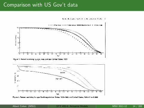
Comparison with US Gov’t data
Albert Cohen (MSU) STT 455-6: Actuarial Models MSU 2011-12 14 / 283
Actuarial Notation
Actuaries make the notational conventions
tpx = P[Tx > t] = Sx(t)
tqx = P[Tx ≤ t] = Fx(t)
u|tqx = P[u < Tx ≤ u + t] = Sx(u)− Sx(u + t)
(13)
u|tqx , also known as the deferred mortality probability, is the probabilitythat (x) survives u years, and then dies in the subsequent t years.
Another convention is that px := 1px and qx := 1qx .
Albert Cohen (MSU) STT 455-6: Actuarial Models MSU 2011-12 15 / 283
Actuarial Notation-Relationships
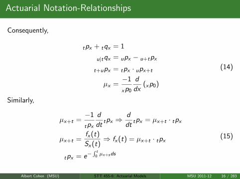
Consequently,
tpx + tqx = 1
u|tqx = upx − u+tpx
t+upx = tpx · upx+t
µx =−1
xp0
d
dx(xp0)
(14)
Similarly,
µx+t =−1
tpx
d
dttpx ⇒
d
dttpx = µx+t · tpx
µx+t =fx(t)
Sx(t)⇒ fx(t) = µx+t · tpx
tpx = e−∫ t
0 µx+sds
(15)
Albert Cohen (MSU) STT 455-6: Actuarial Models MSU 2011-12 16 / 283
Actuarial Notation-Relationships
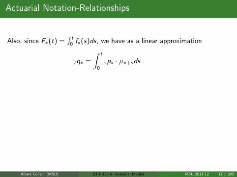
Also, since Fx(t) =∫ t
0 fx(s)ds, we have as a linear approximation
tqx =
∫ t
0spx · µx+sds
qx =
∫ 1
0spx · µx+sds
=
∫ 1
0e−
∫ s0 µx+vdv · µx+sds
≈∫ 1
0µx+sds
≈ µx+ 12
(16)
Albert Cohen (MSU) STT 455-6: Actuarial Models MSU 2011-12 17 / 283
Actuarial Notation-Relationships
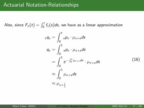
Also, since Fx(t) =∫ t
0 fx(s)ds, we have as a linear approximation
tqx =
∫ t
0spx · µx+sds
qx =
∫ 1
0spx · µx+sds
=
∫ 1
0e−
∫ s0 µx+vdv · µx+sds
≈∫ 1
0µx+sds
≈ µx+ 12
(16)
Albert Cohen (MSU) STT 455-6: Actuarial Models MSU 2011-12 17 / 283
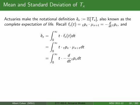
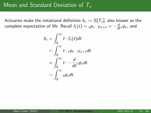
Mean and Standard Deviation of Tx
Actuaries make the notational definition ex := E[Tx ], also known as thecomplete expectation of life. Recall fx(t) = tpx · µx+t = − d
dt tpx , and
ex =
∫ ∞0
t · fx(t)dt
=
∫ ∞0
t · tpx · µx+tdt
=
∫ ∞0
t · − d
dttpxdt
=
∫ ∞0
tpxdt
E[T 2x ] =
∫ ∞0
t2 · fx(t)dt =
∫ ∞0
2t · tpxdt
V [Tx ] := E[T 2x ]− (ex)2
(17)
Albert Cohen (MSU) STT 455-6: Actuarial Models MSU 2011-12 18 / 283
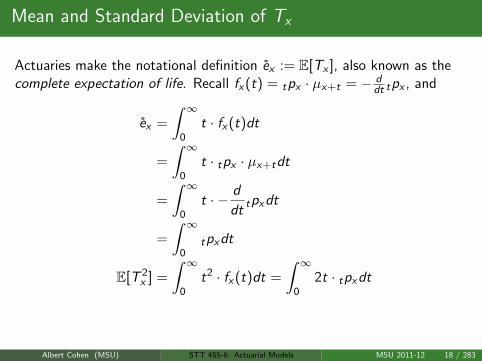
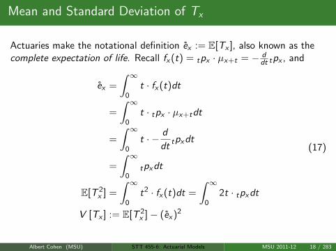
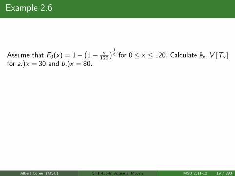
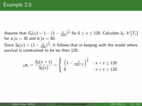
Example 2.6
Assume that F0(x) = 1−(1− x
120
) 16 for 0 ≤ x ≤ 120. Calculate ex ,V [Tx ]
for a.)x = 30 and b.)x = 80.
Since S0(x) =(1− x
120
) 16 , it follows that in keeping with the model where
survival is constrained to be les than 120,
tpx =S0(x + t)
S0(x)=
(
1− t120−x
) 16
: x + t ≤ 120
0 : x + t > 120
Albert Cohen (MSU) STT 455-6: Actuarial Models MSU 2011-12 19 / 283
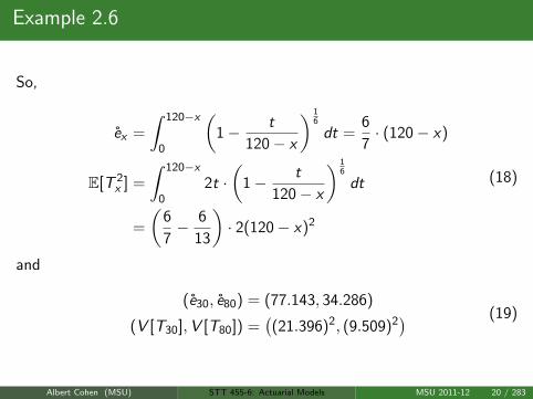
Example 2.6
So,
ex =
∫ 120−x
0
(1− t
120− x
) 16
dt =6
7· (120− x)
E[T 2x ] =
∫ 120−x
02t ·
(1− t
120− x
) 16
dt
=
(6
7− 6
13
)· 2(120− x)2
(18)
and
(e30, e80) = (77.143, 34.286)
(V [T30],V [T80]) =((21.396)2, (9.509)2
) (19)
Albert Cohen (MSU) STT 455-6: Actuarial Models MSU 2011-12 20 / 283

Exam MLC Spring 2007: Q8
Kevin and Kira excel at the newest video game at the local arcade,Reversion. The arcade has only one station for it. Kevin is playing. Kira isnext in line. You are given:
(i) Kevin will play until his parents call him to come home.
(ii) Kira will leave when her parents call her. She will start playing assoon as Kevin leaves if he is called first.
(iii) Each child is subject to a constant force of being called: 0.7 perhour for Kevin; 0.6 per hour for Kira.
(iv) Calls are independent.
(v) If Kira gets to play, she will score points at a rate of 100,000 perhour.
Albert Cohen (MSU) STT 455-6: Actuarial Models MSU 2011-12 21 / 283

Exam MLC Spring 2007: Q8
Calculate the expected number of points Kira will score before she leaves.
(A) 77,000
(B) 80,000
(C) 84,000
(D) 87,000
(E) 90,000
Albert Cohen (MSU) STT 455-6: Actuarial Models MSU 2011-12 22 / 283
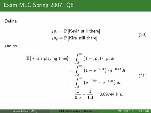
Exam MLC Spring 2007: Q8
Define
tpx = P [Kevin still there]
tpy = P [Kira still there](20)
and so
E [Kira’s playing time] =
∫ ∞0
(1− tpx) · tpydt
=
∫ ∞0
(1− e−0.7t
)· e−0.6tdt
=
∫ ∞0
(e−0.6t − e−1.3t
)dt
=1
0.6− 1
1.3= 0.89744 hrs.
(21)
Albert Cohen (MSU) STT 455-6: Actuarial Models MSU 2011-12 23 / 283
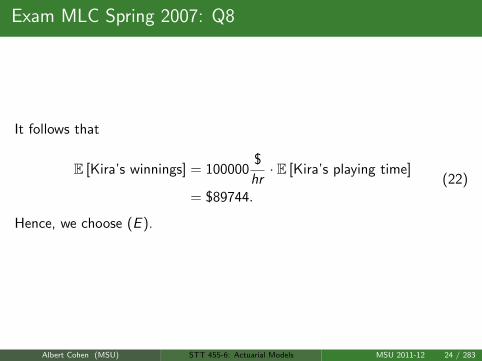
Exam MLC Spring 2007: Q8
It follows that
E [Kira’s winnings] = 100000$
hr· E [Kira’s playing time]
= $89744.(22)
Hence, we choose (E ).
Albert Cohen (MSU) STT 455-6: Actuarial Models MSU 2011-12 24 / 283
Numerical Considerations for Tx
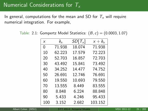
In general, computations for the mean and SD for Tx will requirenumerical integration. For example,
Table: 2.1: Gompertz Model Statistics: (B, c) = (0.0003, 1.07)
x ex SD[Tx ] x + ex0 71.938 18.074 71.93810 62.223 17.579 72.22320 52.703 16.857 72.70330 43.492 15.841 73.49240 34.252 14.477 74.75250 26.691 12.746 76.69160 19.550 10.693 79.55070 13.555 8.449 83.55580 8.848 6.224 88.84890 5.433 4.246 95.433100 3.152 2.682 103.152
Albert Cohen (MSU) STT 455-6: Actuarial Models MSU 2011-12 25 / 283
Curtate Future Lifetime
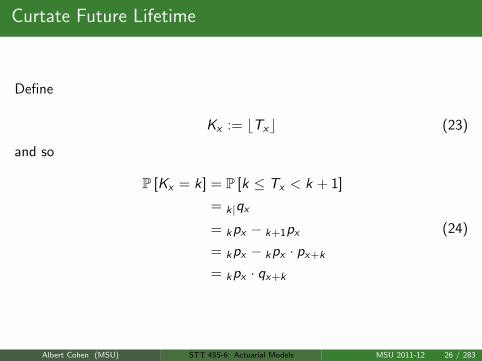
Define
Kx := bTxc (23)
and so
P [Kx = k] = P [k ≤ Tx < k + 1]
= k|qx
= kpx − k+1px
= kpx − kpx · px+k
= kpx · qx+k
(24)
Albert Cohen (MSU) STT 455-6: Actuarial Models MSU 2011-12 26 / 283
Curtate Future Lifetime
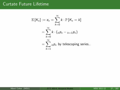
E [Kx ] := ex =∞∑k=0
k · P [Kx = k]
=∞∑k=0
k · (kpx − k+1px)
=∞∑k=1
kpx by telescoping series..
E[K 2x
]=∞∑k=0
k2 · P [Kx = k]
= 2 ·∞∑k=1
k · kpx −∞∑k=1
kpx
= 2 ·∞∑k=1
k · kpx − ex
(25)
Albert Cohen (MSU) STT 455-6: Actuarial Models MSU 2011-12 27 / 283
Curtate Future Lifetime
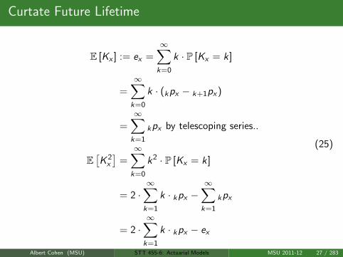
E [Kx ] := ex =∞∑k=0
k · P [Kx = k]
=∞∑k=0
k · (kpx − k+1px)
=∞∑k=1
kpx by telescoping series..
E[K 2x
]=∞∑k=0
k2 · P [Kx = k]
= 2 ·∞∑k=1
k · kpx −∞∑k=1
kpx
= 2 ·∞∑k=1
k · kpx − ex
(25)
Albert Cohen (MSU) STT 455-6: Actuarial Models MSU 2011-12 27 / 283
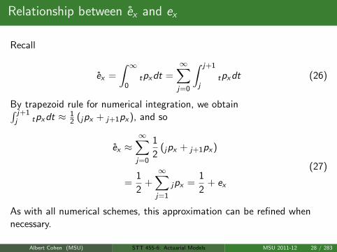
Relationship between ex and ex
Recall
ex =
∫ ∞0
tpxdt =∞∑j=0
∫ j+1
jtpxdt (26)
By trapezoid rule for numerical integration, we obtain∫ j+1j tpxdt ≈ 1
2 (jpx + j+1px), and so
ex ≈∞∑j=0
1
2(jpx + j+1px)
=1
2+∞∑j=1
jpx =1
2+ ex
(27)
As with all numerical schemes, this approximation can be refined whennecessary.
Albert Cohen (MSU) STT 455-6: Actuarial Models MSU 2011-12 28 / 283
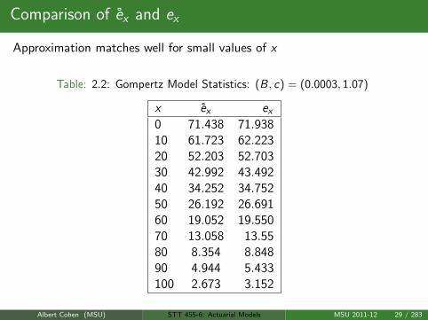
Comparison of ex and ex
Approximation matches well for small values of x
Table: 2.2: Gompertz Model Statistics: (B, c) = (0.0003, 1.07)
x ex ex0 71.438 71.93810 61.723 62.22320 52.203 52.70330 42.992 43.49240 34.252 34.75250 26.192 26.69160 19.052 19.55070 13.058 13.5580 8.354 8.84890 4.944 5.433100 2.673 3.152
Albert Cohen (MSU) STT 455-6: Actuarial Models MSU 2011-12 29 / 283
Notes
An extension of Gompertz - Makeham Laws is the GM(r , s) formulaµx = h1
r (x) + eh2s (x), where h1
r (x), h2s (x) are polynomials of degree r
and s, respectively.
Hazard rate in survival analysis and failure rate in reliability theory isthe same as what actuaries call force of mortality.
Albert Cohen (MSU) STT 455-6: Actuarial Models MSU 2011-12 30 / 283

Homework Questions
HW: 2.1, 2.2, 2.5, 2.6, 2.10, 2.13, 2.14, 2.15
Albert Cohen (MSU) STT 455-6: Actuarial Models MSU 2011-12 31 / 283

Life Tables
Define for a model with maximum age ω and initial age x0 the radix lx0 ,where
lx0+t = lx0 · tpx0 (28)
Albert Cohen (MSU) STT 455-6: Actuarial Models MSU 2011-12 32 / 283

Life Tables
It follows that
lx+t = lx0 · x+t−x0px0
= lx0 · x−x0px0 · tpx
= lx · tpx
tpx =lx+t
lx
(29)
We assume a binomial model where Lt is the number of survivors to agex + t.
Albert Cohen (MSU) STT 455-6: Actuarial Models MSU 2011-12 33 / 283

Life Tables
It follows that
lx+t = lx0 · x+t−x0px0
= lx0 · x−x0px0 · tpx
= lx · tpx
tpx =lx+t
lx
(29)
We assume a binomial model where Lt is the number of survivors to agex + t.
Albert Cohen (MSU) STT 455-6: Actuarial Models MSU 2011-12 33 / 283
Life Tables
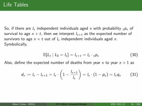
So, if there are lx independent individuals aged x with probability tpx ofsurvival to age x + t, then we interpret lx+t as the expected number ofsurvivors to age x + t out of lx independent individuals aged x .Symbolically,
E[Lt | L0 = lx ] = lx+t = lx · tpx (30)
Also, define the expected number of deaths from year x to year x + 1 as
dx := lx − lx+1 = lx ·(
1− lx+1
lx
)= lx · (1− px) = lxqx (31)
Albert Cohen (MSU) STT 455-6: Actuarial Models MSU 2011-12 34 / 283
Life Tables
So, if there are lx independent individuals aged x with probability tpx ofsurvival to age x + t, then we interpret lx+t as the expected number ofsurvivors to age x + t out of lx independent individuals aged x .Symbolically,
E[Lt | L0 = lx ] = lx+t = lx · tpx (30)
Also, define the expected number of deaths from year x to year x + 1 as
dx := lx − lx+1 = lx ·(
1− lx+1
lx
)= lx · (1− px) = lxqx (31)
Albert Cohen (MSU) STT 455-6: Actuarial Models MSU 2011-12 34 / 283
Example 3.1
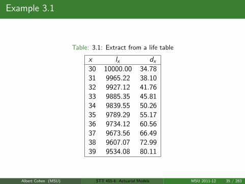
Table: 3.1: Extract from a life table
x lx dx
30 10000.00 34.7831 9965.22 38.1032 9927.12 41.7633 9885.35 45.8134 9839.55 50.2635 9789.29 55.1736 9734.12 60.5637 9673.56 66.4938 9607.07 72.9939 9534.08 80.11
Albert Cohen (MSU) STT 455-6: Actuarial Models MSU 2011-12 35 / 283

Example 3.1
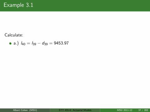
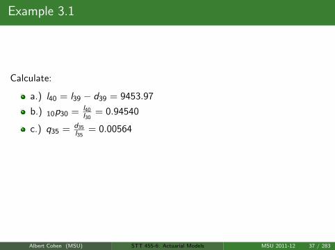
Calculate:
a.) l40
b.) 10p30
c.) q35
d.) 5q30
e.) P [(30) dies between age 35 and 36]
Albert Cohen (MSU) STT 455-6: Actuarial Models MSU 2011-12 36 / 283
Example 3.1
Calculate:
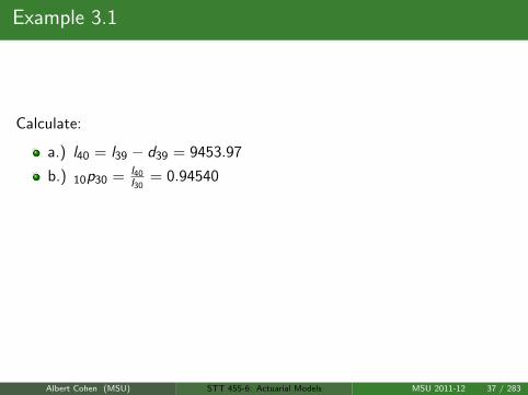
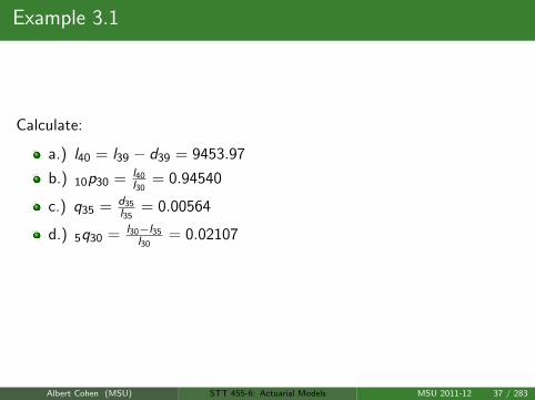
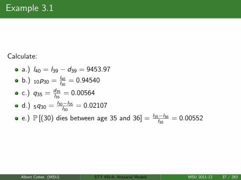
a.) l40 = l39 − d39 = 9453.97
b.) 10p30 = l40l30
= 0.94540
c.) q35 = d35l35
= 0.00564
d.) 5q30 = l30−l35l30
= 0.02107
e.) P [(30) dies between age 35 and 36] = l35−l36l30
= 0.00552
Albert Cohen (MSU) STT 455-6: Actuarial Models MSU 2011-12 37 / 283
Example 3.1
Calculate:
a.) l40 = l39 − d39 = 9453.97
b.) 10p30 = l40l30
= 0.94540
c.) q35 = d35l35
= 0.00564
d.) 5q30 = l30−l35l30
= 0.02107
e.) P [(30) dies between age 35 and 36] = l35−l36l30
= 0.00552
Albert Cohen (MSU) STT 455-6: Actuarial Models MSU 2011-12 37 / 283
Example 3.1
Calculate:
a.) l40 = l39 − d39 = 9453.97
b.) 10p30 = l40l30
= 0.94540
c.) q35 = d35l35
= 0.00564
d.) 5q30 = l30−l35l30
= 0.02107
e.) P [(30) dies between age 35 and 36] = l35−l36l30
= 0.00552
Albert Cohen (MSU) STT 455-6: Actuarial Models MSU 2011-12 37 / 283
Example 3.1
Calculate:
a.) l40 = l39 − d39 = 9453.97
b.) 10p30 = l40l30
= 0.94540
c.) q35 = d35l35
= 0.00564
d.) 5q30 = l30−l35l30
= 0.02107
e.) P [(30) dies between age 35 and 36] = l35−l36l30
= 0.00552
Albert Cohen (MSU) STT 455-6: Actuarial Models MSU 2011-12 37 / 283
Example 3.1
Calculate:
a.) l40 = l39 − d39 = 9453.97
b.) 10p30 = l40l30
= 0.94540
c.) q35 = d35l35
= 0.00564
d.) 5q30 = l30−l35l30
= 0.02107
e.) P [(30) dies between age 35 and 36] = l35−l36l30
= 0.00552
Albert Cohen (MSU) STT 455-6: Actuarial Models MSU 2011-12 37 / 283
Fractional Age Assumptions
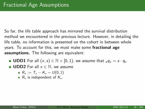
So far, the life table approach has mirrored the survival distributionmethod we encountered in the previous lecture. However, in detailing thelife table, no information is presented on the cohort in between wholeyears. To account for this, we must make some fractional ageassumptions. The following are equivalent:
UDD1 For all (x , s) ∈ N× [0, 1), we assume that sqx = s · qx
UDD2 For all x ∈ N, we assume
Rx := Tx − Kx ∼ U(0, 1)Rx is independent of Kx .
Albert Cohen (MSU) STT 455-6: Actuarial Models MSU 2011-12 38 / 283
Fractional Age Assumptions
So far, the life table approach has mirrored the survival distributionmethod we encountered in the previous lecture. However, in detailing thelife table, no information is presented on the cohort in between wholeyears. To account for this, we must make some fractional ageassumptions. The following are equivalent:
UDD1 For all (x , s) ∈ N× [0, 1), we assume that sqx = s · qx
UDD2 For all x ∈ N, we assume
Rx := Tx − Kx ∼ U(0, 1)Rx is independent of Kx .
Albert Cohen (MSU) STT 455-6: Actuarial Models MSU 2011-12 38 / 283
Proof of Equivalence
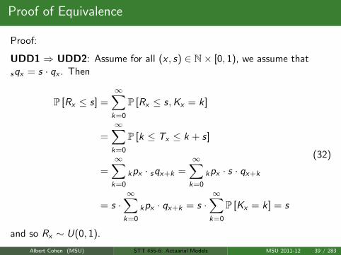
Proof:
UDD1 ⇒ UDD2: Assume for all (x , s) ∈ N× [0, 1), we assume that
sqx = s · qx . Then
P [Rx ≤ s] =∞∑k=0
P [Rx ≤ s,Kx = k]
=∞∑k=0
P [k ≤ Tx ≤ k + s]
=∞∑k=0
kpx · sqx+k =∞∑k=0
kpx · s · qx+k
= s ·∞∑k=0
kpx · qx+k = s ·∞∑k=0
P [Kx = k] = s
(32)
and so Rx ∼ U(0, 1).
Albert Cohen (MSU) STT 455-6: Actuarial Models MSU 2011-12 39 / 283
Proof of Equivalence
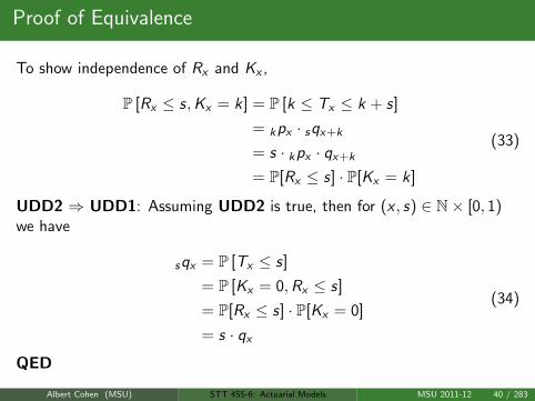
To show independence of Rx and Kx ,
P [Rx ≤ s,Kx = k] = P [k ≤ Tx ≤ k + s]
= kpx · sqx+k
= s · kpx · qx+k
= P[Rx ≤ s] · P[Kx = k]
(33)
UDD2 ⇒ UDD1: Assuming UDD2 is true, then for (x , s) ∈ N× [0, 1)we have
sqx = P [Tx ≤ s]
= P [Kx = 0,Rx ≤ s]
= P[Rx ≤ s] · P[Kx = 0]
= s · qx
(34)
QED
Albert Cohen (MSU) STT 455-6: Actuarial Models MSU 2011-12 40 / 283

Corollary
Recall that sqx = lx−lx+s
lx. It follows now that
sqx = sqx = sdx
lx=
lx − lx+s
lx
lx+s = lx − s · dx
which is a linear decreasing function of s ∈ [0, 1)
qx =d
ds[sqx ] = fx(s) = spx · µx+s
(35)
But, since qx is constant in s, we have fx(s) is constant for s ∈ [0, 1).
Read over Examples 3.2− 3.5
Albert Cohen (MSU) STT 455-6: Actuarial Models MSU 2011-12 41 / 283

Corollary
Recall that sqx = lx−lx+s
lx. It follows now that
sqx = sqx = sdx
lx=
lx − lx+s
lxlx+s = lx − s · dx
which is a linear decreasing function of s ∈ [0, 1)
qx =d
ds[sqx ] = fx(s) = spx · µx+s
(35)
But, since qx is constant in s, we have fx(s) is constant for s ∈ [0, 1).
Read over Examples 3.2− 3.5
Albert Cohen (MSU) STT 455-6: Actuarial Models MSU 2011-12 41 / 283
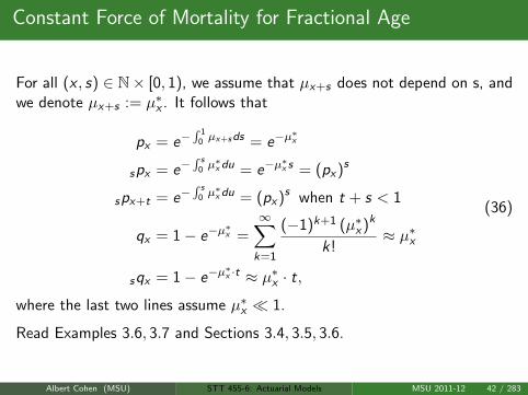
Constant Force of Mortality for Fractional Age
For all (x , s) ∈ N× [0, 1), we assume that µx+s does not depend on s, andwe denote µx+s := µ∗x . It follows that
px = e−∫ 1
0 µx+sds = e−µ∗x
spx = e−∫ s
0 µ∗x du = e−µ
∗x s = (px)s
spx+t = e−∫ s
0 µ∗x du = (px)s when t + s < 1
qx = 1− e−µ∗x =
∞∑k=1
(−1)k+1 (µ∗x)k
k!≈ µ∗x
sqx = 1− e−µ∗x ·t ≈ µ∗x · t,
(36)
where the last two lines assume µ∗x 1.
Read Examples 3.6, 3.7 and Sections 3.4, 3.5, 3.6.
Albert Cohen (MSU) STT 455-6: Actuarial Models MSU 2011-12 42 / 283

Homework Questions
HW: 3.1, 3.2, 3.4, 3.7, 3.8, 3.9, 3.10
Albert Cohen (MSU) STT 455-6: Actuarial Models MSU 2011-12 43 / 283

Contingent Events
We have spent the previous two lectures on modeling human mortality.The need for such models in insurance pricing arises when designingcontracts that are event-contingent. Such events include reachingretirement before the end of the underlying life (x) .
However, one can also write contracts that are dependent on a life (x)being admitted to college (planning for school), and also on (x)
′s externalportfolios maintaining a minimal value over a time-interval (insuringexternal investments.)
Albert Cohen (MSU) STT 455-6: Actuarial Models MSU 2011-12 44 / 283
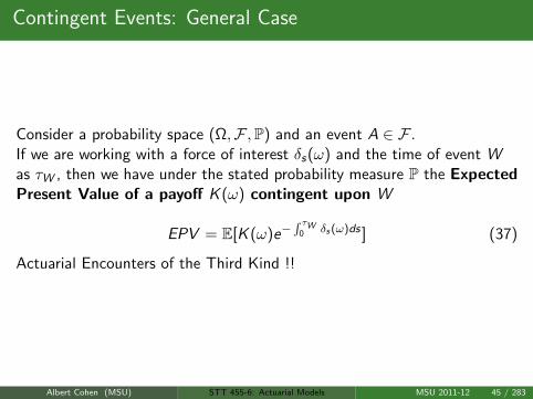
Contingent Events: General Case
Consider a probability space (Ω,F ,P) and an event A ∈ F .If we are working with a force of interest δs(ω) and the time of event Was τW , then we have under the stated probability measure P the ExpectedPresent Value of a payoff K (ω) contingent upon W
EPV = E[K (ω)e−∫ τW
0 δs(ω)ds ] (37)
Actuarial Encounters of the Third Kind !!
Albert Cohen (MSU) STT 455-6: Actuarial Models MSU 2011-12 45 / 283
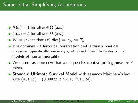
Some Initial Simplifying Assumptions
K (ω) = 1 for all ω ∈ Ω (a.s.)
δs(ω) = δ for all ω ∈ Ω (a.s.)
W := event that (x) dies ⇒ τW := Tx
P is obtained via historical observation and is thus a physicalmeasure. Specifically, we use tpx obtained from life tables or viamodels of human mortality
We do not assume now that a unique risk-neutral pricing measure Pexists.
Standard Ultimate Survival Model with assumes Makeham’s lawwith (A,B, c) = (0.00022, 2.7× 10⁻⁶, 1.124)
Albert Cohen (MSU) STT 455-6: Actuarial Models MSU 2011-12 46 / 283
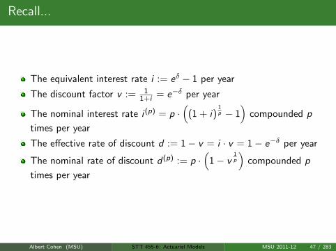
Recall...
The equivalent interest rate i := eδ − 1 per year
The discount factor v := 11+i = e−δ per year
The nominal interest rate i (p) = p ·(
(1 + i)1p − 1
)compounded p
times per year
The effective rate of discount d := 1− v = i · v = 1− e−δ per year
The nominal rate of discount d (p) := p ·(
1− v1p
)compounded p
times per year
Albert Cohen (MSU) STT 455-6: Actuarial Models MSU 2011-12 47 / 283
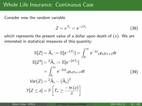
Whole Life Insurance: Continuous Case
Consider now the random variable
Z = vTx = e−δTx (38)
which represents the present value of a dollar upon death of (x). We areinterested in statistical measures of this quantity:
E[Z ] = Ax := E[e−δTx ] =
∫ ∞0
e−δt tpxµx+tdt
E[Z 2] = 2Ax := E[e−2δTx ]
=
∫ ∞0
e−2δttpxµx+tdt
Var(Z ) = 2Ax −(Ax
)2
P[Z ≤ z ] = P[
Tx ≥− ln (z)
δ
](39)
Albert Cohen (MSU) STT 455-6: Actuarial Models MSU 2011-12 48 / 283
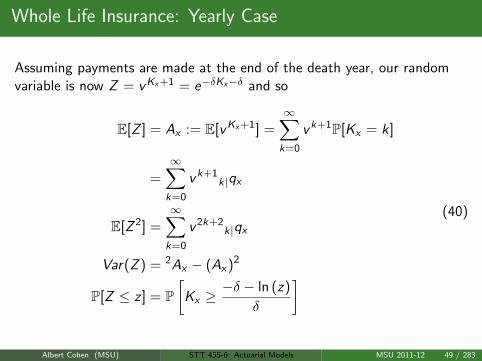
Whole Life Insurance: Yearly Case
Assuming payments are made at the end of the death year, our randomvariable is now Z = vKx+1 = e−δKx−δ and so
E[Z ] = Ax := E[vKx+1] =∞∑k=0
vk+1P[Kx = k]
=∞∑k=0
vk+1k|qx
E[Z 2] =∞∑k=0
v 2k+2k|qx
Var(Z ) = 2Ax − (Ax)2
P[Z ≤ z ] = P[
Kx ≥−δ − ln (z)
δ
](40)
Albert Cohen (MSU) STT 455-6: Actuarial Models MSU 2011-12 49 / 283
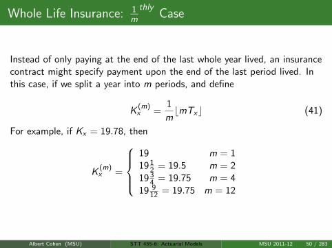
Whole Life Insurance: 1m
thlyCase
Instead of only paying at the end of the last whole year lived, an insurancecontract might specify payment upon the end of the last period lived. Inthis case, if we split a year into m periods, and define
K(m)x =
1
mbmTxc (41)
For example, if Kx = 19.78, then
K(m)x =
19 m = 119 1
2 = 19.5 m = 219 3
4 = 19.75 m = 419 9
12 = 19.75 m = 12
Albert Cohen (MSU) STT 455-6: Actuarial Models MSU 2011-12 50 / 283
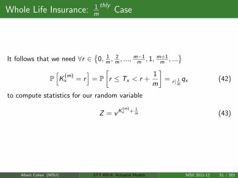
Whole Life Insurance: 1m
thlyCase
It follows that we need ∀r ∈
0, 1m ,
2m , ...,
m−1m , 1, m+1
m , ...
P[K
(m)x = r
]= P
[r ≤ Tx < r +
1
m
]= r | 1
mqx (42)
to compute statistics for our random variable
Z = vK(m)x + 1
m (43)
Albert Cohen (MSU) STT 455-6: Actuarial Models MSU 2011-12 51 / 283
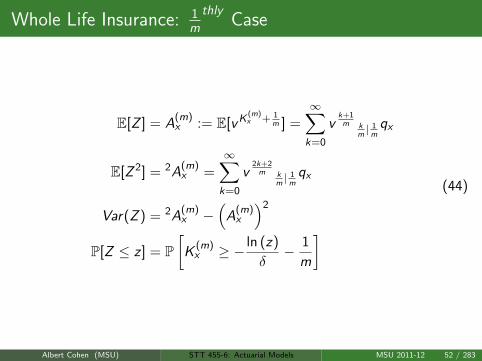
Whole Life Insurance: 1m
thlyCase
E[Z ] = A(m)x := E[vK
(m)x + 1
m ] =∞∑k=0
vk+1m k
m| 1m
qx
E[Z 2] = 2A(m)x =
∞∑k=0
v2k+2m k
m| 1m
qx
Var(Z ) = 2A(m)x −
(A
(m)x
)2
P[Z ≤ z ] = P[
K(m)x ≥ − ln (z)
δ− 1
m
](44)
Albert Cohen (MSU) STT 455-6: Actuarial Models MSU 2011-12 52 / 283

Recursion Method
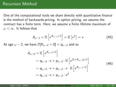
One of the computational tools we share directly with quantitative financeis the method of backwards-pricing. In option pricing, we assume thecontract has a finite term. Here, we assume a finite lifetime maximum ofω <∞. It follows that
Aω−1 = E[vKω−1+1
]= E
[v 1]
= v (45)
At age ω − 2, we have P[Kω−2 = 0] = qω−2 and so
Aω−2 = E[vKω−2+1
]= qω−2 · v + pω−2 · E
[v (1+Kω−1)+1
]= qω−2 · v + pω−2 · v · E
[vKω−1+1
]= qω−2 · v + pω−2 · v 2
(46)
Albert Cohen (MSU) STT 455-6: Actuarial Models MSU 2011-12 53 / 283
Recursion Method
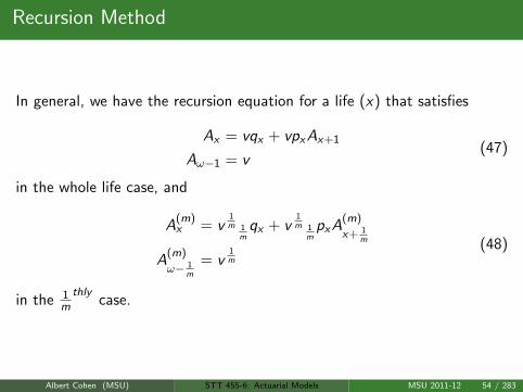
In general, we have the recursion equation for a life (x) that satisfies
Ax = vqx + vpxAx+1
Aω−1 = v(47)
in the whole life case, and
A(m)x = v
1m 1
mqx + v
1m 1
mpxA
(m)
x+ 1m
A(m)
ω− 1m
= v1m
(48)
in the 1m
thlycase.
Albert Cohen (MSU) STT 455-6: Actuarial Models MSU 2011-12 54 / 283
Recursion Method
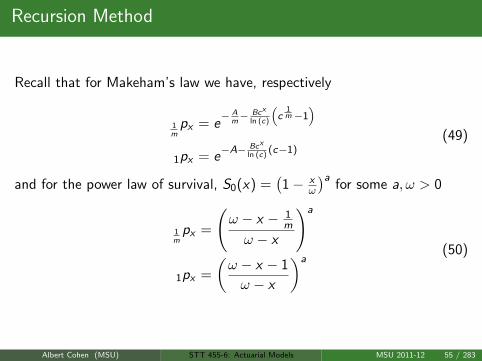
Recall that for Makeham’s law we have, respectively
1m
px = e− A
m− Bcx
ln (c)
(c
1m−1
)
1px = e−A− Bcx
ln (c)(c−1)
(49)
and for the power law of survival, S0(x) =(1− x
ω
)afor some a, ω > 0
1m
px =
(ω − x − 1
m
ω − x
)a
1px =
(ω − x − 1
ω − x
)a(50)
Albert Cohen (MSU) STT 455-6: Actuarial Models MSU 2011-12 55 / 283
Recursion Method
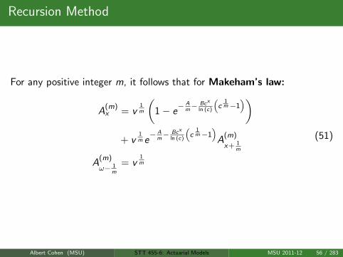
For any positive integer m, it follows that for Makeham’s law:
A(m)x = v
1m
(1− e
− Am− Bcx
ln (c)
(c
1m−1
))+ v
1m e− A
m− Bcx
ln (c)
(c
1m−1
)A
(m)
x+ 1m
A(m)
ω− 1m
= v1m
(51)
Albert Cohen (MSU) STT 455-6: Actuarial Models MSU 2011-12 56 / 283

Recursion Method
For any positive integer m, it follows that for Power law:
A(m)x = v
1m
(1−
(ω − x − 1
m
ω − x
)a)
+ v1m
(ω − x − 1
m
ω − x
)a
A(m)
x+ 1m
A(m)
ω− 1m
= v1m
(52)
HW Project: For Power law with a = 35 and ω = 101
Generate a spreadsheet like Table 4.1 in the text, including values for2A
(m)x
Repeat Example 4.3 with the Power law model
Albert Cohen (MSU) STT 455-6: Actuarial Models MSU 2011-12 57 / 283
Term Insurance: Continuous Case
Consider now the case where payment is made in the continuous case, anddeath benefit is payable to the policyholder only if Tx ≤ n. Then, we areinterested in the random variable
Z = e−δTx 1Tx≤n (53)
and so
A1x :n = E[Z ] =
∫ n
0e−δt tpxµx+tdt
2A1x :n = E
[Z 2]
=
∫ n
0e−2δt
tpxµx+tdt
(54)
Albert Cohen (MSU) STT 455-6: Actuarial Models MSU 2011-12 58 / 283
Term Insurance: 1m
thlyCase
Consider again the case where the death benefit is payable at the end of
the 1m
thlyperiod in the death year to the policyholder only if
K(m)x + 1
m ≤ n. Then, we are interested in the random variable
Z = e−δ(K(m)x + 1
m)1
K(m)x + 1
m≤n (55)
and so
A(m)1x :n = E[Z ] =
mn−1∑k=0
vk+1m k
m| 1m
qx
2A(m)1x :n = E
[Z 2]
=mn−1∑k=0
v2k+2m k
m| 1m
qx
(56)
Albert Cohen (MSU) STT 455-6: Actuarial Models MSU 2011-12 59 / 283
Pure Endowment
Pure endowment benefits depend on the survival policyholder (x) until atleast age x + n. In such a contract, a fixed benefit of 1 is paid at time n.This is expressed via
Z = e−δn1Tx≥n
A 1x :n = E[Z ] = vn
npx
= e−δnnpx
(57)
Albert Cohen (MSU) STT 455-6: Actuarial Models MSU 2011-12 60 / 283
Endowment Insurance
Endowment insurance is a combination of term insurance and pureendowment. In such a policy, the amount is paid upon death if it occurswith a fixed term n. However, if (x) survives beyond n years, the suminsured is payable at the end of the nth year. The corresponding presentvalue random variable is
Z = e−δminTx ,n
E[Z ] = Ax :n
=
∫ n
0e−δt tpxµx+tdt + e−δnnpx
= A1x :n + A 1
x :n
(58)
This can be generalized once again to the 1m
thlycase and for E[Z 2]
Albert Cohen (MSU) STT 455-6: Actuarial Models MSU 2011-12 61 / 283
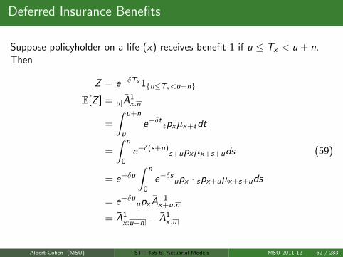
Deferred Insurance Benefits
Suppose policyholder on a life (x) receives benefit 1 if u ≤ Tx < u + n.Then
Z = e−δTx 1u≤Tx<u+n
E[Z ] = u|A1x :n
=
∫ u+n
ue−δt tpxµx+tdt
=
∫ n
0e−δ(s+u)
s+upxµx+s+uds
= e−δu∫ n
0e−δsupx · spx+uµx+s+uds
= e−δuupx A 1x+u:n
= A1x :u+n − A1
x :u
(59)
Albert Cohen (MSU) STT 455-6: Actuarial Models MSU 2011-12 62 / 283

Relationships
By definition, we have
Ax = A1x :n + n|Ax
= A1x :n + vn
npxAx+n
(60)
What about relationship between Ax and Ax?
Albert Cohen (MSU) STT 455-6: Actuarial Models MSU 2011-12 63 / 283

Relationships
By definition, we have
Ax = A1x :n + n|Ax
= A1x :n + vn
npxAx+n
(60)
What about relationship between Ax and Ax?
Albert Cohen (MSU) STT 455-6: Actuarial Models MSU 2011-12 63 / 283
Employing UDD: Ax vs Ax
If expected values are computed via information derived from life tables,then certainly Ax must be approximated using techniques from previouslecture.
Recall that by the definition of spx and the UDD, we have
spxµx+s = fx(s)
=d
dsP[Tx ≤ s]
=d
ds(sqx) =
d
ds(s · qx)
= qx
(61)
Albert Cohen (MSU) STT 455-6: Actuarial Models MSU 2011-12 64 / 283
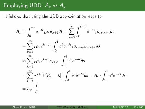
Employing UDD: Ax vs Ax
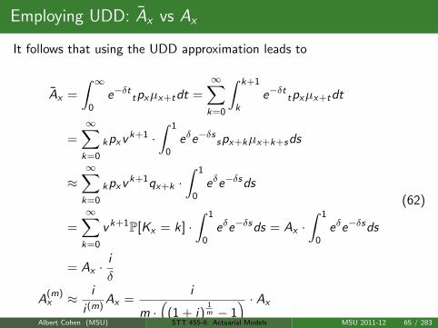
It follows that using the UDD approximation leads to
Ax =
∫ ∞0
e−δt tpxµx+tdt =∞∑k=0
∫ k+1
ke−δt tpxµx+tdt
=∞∑k=0
kpxvk+1 ·∫ 1
0eδe−δs spx+kµx+k+sds
≈∞∑k=0
kpxvk+1qx+k ·∫ 1
0eδe−δsds
=∞∑k=0
vk+1P[Kx = k] ·∫ 1
0eδe−δsds = Ax ·
∫ 1
0eδe−δsds
= Ax ·i
δ
A(m)x ≈ i
i (m)Ax =
i
m ·(
(1 + i)1m − 1
) · Ax
(62)
Albert Cohen (MSU) STT 455-6: Actuarial Models MSU 2011-12 65 / 283
Employing UDD: Ax vs Ax
It follows that using the UDD approximation leads to
Ax =
∫ ∞0
e−δt tpxµx+tdt =∞∑k=0
∫ k+1
ke−δt tpxµx+tdt
=∞∑k=0
kpxvk+1 ·∫ 1
0eδe−δs spx+kµx+k+sds
≈∞∑k=0
kpxvk+1qx+k ·∫ 1
0eδe−δsds
=∞∑k=0
vk+1P[Kx = k] ·∫ 1
0eδe−δsds = Ax ·
∫ 1
0eδe−δsds
= Ax ·i
δ
A(m)x ≈ i
i (m)Ax =
i
m ·(
(1 + i)1m − 1
) · Ax
(62)
Albert Cohen (MSU) STT 455-6: Actuarial Models MSU 2011-12 65 / 283
Claims Accelaration Approach : A(m)x vs Ax
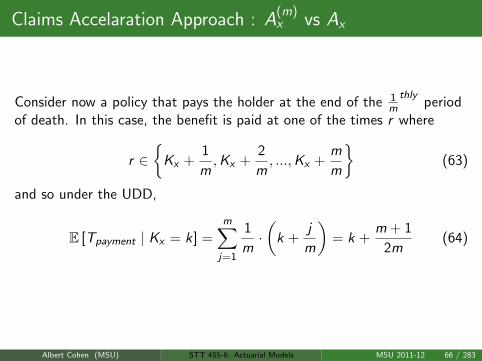
Consider now a policy that pays the holder at the end of the 1m
thlyperiod
of death. In this case, the benefit is paid at one of the times r where
r ∈
Kx +1
m,Kx +
2
m, ...,Kx +
m
m
(63)
and so under the UDD,
E [Tpayment | Kx = k] =m∑j=1
1
m·(
k +j
m
)= k +
m + 1
2m(64)
Albert Cohen (MSU) STT 455-6: Actuarial Models MSU 2011-12 66 / 283
Claims Accelaration Approach : A(m)x vs Ax
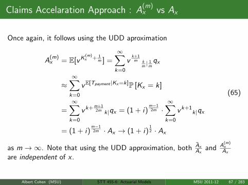
Once again, it follows using the UDD aproximation
A(m)x = E[vK
(m)x + 1
m ] =∞∑k=0
vk+1m k
m| 1m
qx
≈∞∑k=0
vE[Tpayment |Kx=k]P [Kx = k]
=∞∑k=0
vk+m+12m k|qx = (1 + i)
m−12m ·
∞∑k=0
vk+1k|qx
= (1 + i)m−12m · Ax → (1 + i)
12 · Ax
(65)
as m→∞. Note that using the UDD approximation, both AxAx
and A(m)xAx
are independent of x .
Albert Cohen (MSU) STT 455-6: Actuarial Models MSU 2011-12 67 / 283
Variable Insurance Benefits
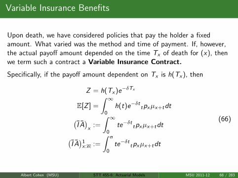
Upon death, we have considered policies that pay the holder a fixedamount. What varied was the method and time of payment. If, however,the actual payoff amount depended on the time Tx of death for (x), thenwe term such a contract a Variable Insurance Contract.
Specifically, if the payoff amount dependent on Tx is h(Tx), then
Z = h(Tx)e−δTx
E[Z ] =
∫ ∞0
h(t)e−δt tpxµx+tdt(I A)x
:=
∫ ∞0
te−δt tpxµx+tdt(I A)
1x :n :=
∫ n
0te−δt tpxµx+tdt
(66)
Albert Cohen (MSU) STT 455-6: Actuarial Models MSU 2011-12 68 / 283
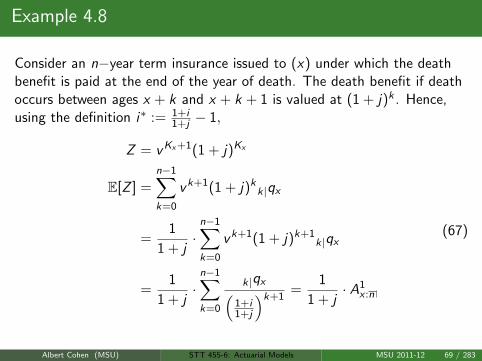
Example 4.8
Consider an n−year term insurance issued to (x) under which the deathbenefit is paid at the end of the year of death. The death benefit if deathoccurs between ages x + k and x + k + 1 is valued at (1 + j)k . Hence,using the definition i∗ := 1+i
1+j − 1,
Z = vKx+1(1 + j)Kx
E[Z ] =n−1∑k=0
vk+1(1 + j)kk|qx
=1
1 + j·n−1∑k=0
vk+1(1 + j)k+1k|qx
=1
1 + j·n−1∑k=0
k|qx(1+i1+j
)k+1=
1
1 + j· A1
x :n
(67)
Albert Cohen (MSU) STT 455-6: Actuarial Models MSU 2011-12 69 / 283

Homework Questions
HW: 4.1, 4.2, 4.3, 4.7, 4.9, 4.11, 4.12, 4.14, 4.15, 4.16, 4.17, 4.18
Albert Cohen (MSU) STT 455-6: Actuarial Models MSU 2011-12 70 / 283
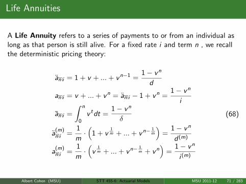
Life Annuities
A Life Annuity refers to a series of payments to or from an individual aslong as that person is still alive. For a fixed rate i and term n , we recallthe deterministic pricing theory:
an i = 1 + v + ...+ vn−1 =1− vn
d
an i = v + ...+ vn = an i − 1 + vn =1− vn
i
an i =
∫ n
0v tdt =
1− vn
δ
a(m)n i =
1
m·(
1 + v1m + ...+ vn− 1
m
)=
1− vn
d (m)
a(m)n i =
1
m·(
v1m + ...+ vn− 1
m + vn)
=1− vn
i (m)
(68)
Albert Cohen (MSU) STT 455-6: Actuarial Models MSU 2011-12 71 / 283
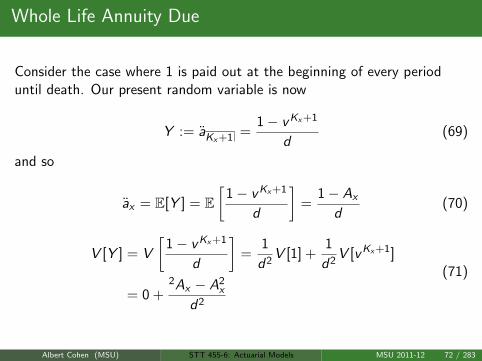
Whole Life Annuity Due
Consider the case where 1 is paid out at the beginning of every perioduntil death. Our present random variable is now
Y := aKx+1 =1− vKx+1
d(69)
and so
ax = E[Y ] = E[
1− vKx+1
d
]=
1− Ax
d(70)
V [Y ] = V
[1− vKx+1
d
]=
1
d2V [1] +
1
d2V [vKx+1]
= 0 +2Ax − A2
x
d2
(71)
Albert Cohen (MSU) STT 455-6: Actuarial Models MSU 2011-12 72 / 283
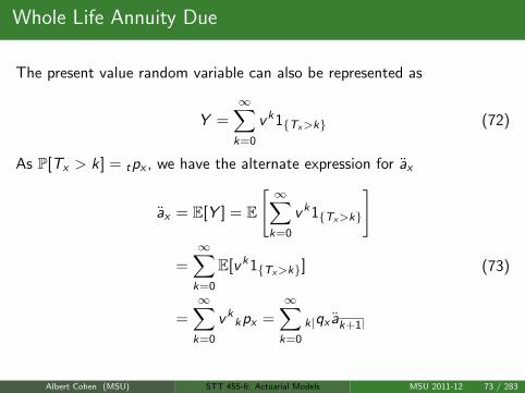
Whole Life Annuity Due
The present value random variable can also be represented as
Y =∞∑k=0
vk1Tx>k (72)
As P[Tx > k] = tpx , we have the alternate expression for ax
ax = E[Y ] = E
[ ∞∑k=0
vk1Tx>k
]
=∞∑k=0
E[vk1Tx>k]
=∞∑k=0
vkkpx =
∞∑k=0
k|qx ak+1
(73)
Albert Cohen (MSU) STT 455-6: Actuarial Models MSU 2011-12 73 / 283
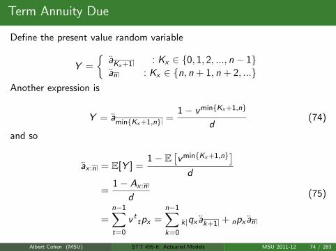
Term Annuity Due
Define the present value random variable
Y =
aKx+1 : Kx ∈ 0, 1, 2, ..., n − 1an : Kx ∈ n, n + 1, n + 2, ...
Another expression is
Y = aminKx+1,n =1− v minKx+1,n
d(74)
and so
ax :n = E[Y ] =1− E
[v minKx+1,n]
d
=1− Ax :n
d
=n−1∑t=0
v ttpx =
n−1∑k=0
k|qx ak+1 + npx an
(75)
Albert Cohen (MSU) STT 455-6: Actuarial Models MSU 2011-12 74 / 283
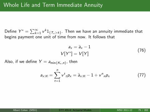
Whole Life and Term Immediate Annuity
Define Y ∗ =∑∞
k=1 vk1Tx>k. Then we have an annuity immediate thatbegins payment one unit of time from now. It follows that
ax = ax − 1
V [Y ∗] = V [Y ](76)
Also, if we define Y = aminKx ,n, then
ax :n =n∑
t=1
v ttpx = ax :n − 1 + vn
npx (77)
Albert Cohen (MSU) STT 455-6: Actuarial Models MSU 2011-12 75 / 283
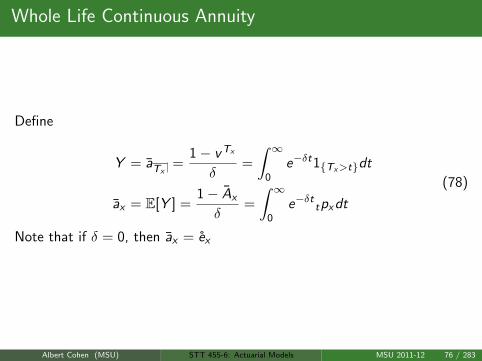
Whole Life Continuous Annuity
Define
Y = aTx=
1− vTx
δ=
∫ ∞0
e−δt1Tx>tdt
ax = E[Y ] =1− Ax
δ=
∫ ∞0
e−δt tpxdt
(78)
Note that if δ = 0, then ax = ex
Albert Cohen (MSU) STT 455-6: Actuarial Models MSU 2011-12 76 / 283
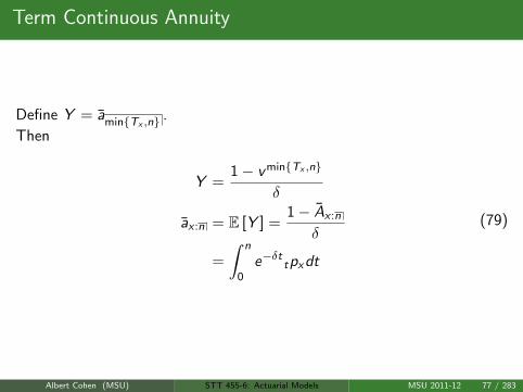
Term Continuous Annuity
Define Y = aminTx ,n .
Then
Y =1− v minTx ,n
δ
ax :n = E [Y ] =1− Ax :n
δ
=
∫ n
0e−δt tpxdt
(79)
Albert Cohen (MSU) STT 455-6: Actuarial Models MSU 2011-12 77 / 283
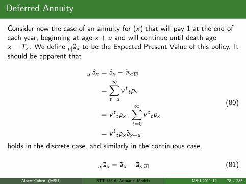
Deferred Annuity
Consider now the case of an annuity for (x) that will pay 1 at the end ofeach year, beginning at age x + u and will continue until death agex + Tx . We define u|ax to be the Expected Present Value of this policy. Itshould be apparent that
u|ax = ax − ax :u
=∞∑t=u
v ttpx
= v ttpx ·
∞∑t=0
v ttpx
= v ttpx ax+u
(80)
holds in the discrete case, and similarly in the continuous case,
u|ax = ax − ax :u (81)
Albert Cohen (MSU) STT 455-6: Actuarial Models MSU 2011-12 78 / 283
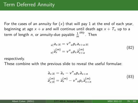
Term Deferred Annuity
For the cases of an annuity for (x) that will pay 1 at the end of each year,beginning at age x + u and will continue until death age x + Tx up to a
term of length n, or annuity-due payable 1m
thly. Then
u|ax :n = vuupxax+u:n
u|a(m)x = vu
upx a(m)x+u
(82)
respectively.These combine with the previous slide to reveal the useful formulae:
ax :n = ax − vnnpx ax+n
a(m)x :n = a
(m)x − vn
npx a(m)x+n
(83)
Albert Cohen (MSU) STT 455-6: Actuarial Models MSU 2011-12 79 / 283
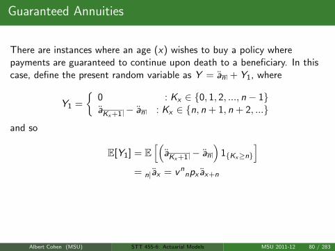
Guaranteed Annuities
There are instances where an age (x) wishes to buy a policy wherepayments are guaranteed to continue upon death to a beneficiary. In thiscase, define the present random variable as Y = an + Y1, where
Y1 =
0 : Kx ∈ 0, 1, 2, ..., n − 1aKx+1 − an : Kx ∈ n, n + 1, n + 2, ...
and so
E[Y1] = E[(
aKx+1 − an)
1Kx≥n
]= n|ax = vn
npx ax+n
E[Y ] := ax :n = an + vnnpx ax+n
and E[Y (m)] := a(m)
x :n= a
(m)n + vn
npx a(m)x+n
(84)
Albert Cohen (MSU) STT 455-6: Actuarial Models MSU 2011-12 80 / 283
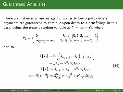

Example 5.4
A pension plan member is entitled to a benefit of 1000 per month, inadvance, for life from age 65, with no guarantee. She can opt to take alower benefit with a 10−year guarantee. The revised benefit is calculatedto have equal EPV at age 65 to the original benefit. Calculate the revisedbenefit using the Standard Ultimate Survival Model, with interest at 5%per year.
Albert Cohen (MSU) STT 455-6: Actuarial Models MSU 2011-12 81 / 283
Example 5.4
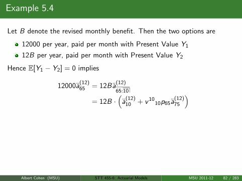
Let B denote the revised monthly benefit. Then the two options are
12000 per year, paid per month with Present Value Y1
12B per year, paid per month with Present Value Y2
Hence E[Y1 − Y2] = 0 implies
12000a(12)65 = 12Ba
(12)
65:10
= 12B ·(
a(12)10 + v 10
10p65a(12)75
)
∴ B = 1000 ·a
(12)65
a(12)10 + v 10
10p65a(12)75
= 1000 · 13.0870
13.3791= 978.17
V [Y1 − Y2] = 0?
(85)
Albert Cohen (MSU) STT 455-6: Actuarial Models MSU 2011-12 82 / 283
Example 5.4
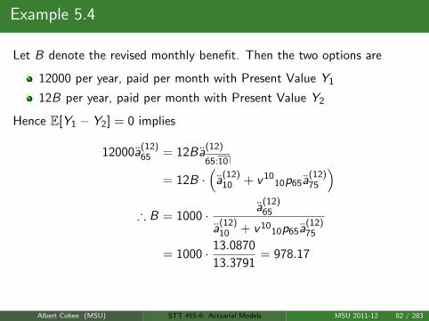
Let B denote the revised monthly benefit. Then the two options are
12000 per year, paid per month with Present Value Y1
12B per year, paid per month with Present Value Y2
Hence E[Y1 − Y2] = 0 implies
12000a(12)65 = 12Ba
(12)
65:10
= 12B ·(
a(12)10 + v 10
10p65a(12)75
)∴ B = 1000 ·
a(12)65
a(12)10 + v 10
10p65a(12)75
= 1000 · 13.0870
13.3791= 978.17
V [Y1 − Y2] = 0?
(85)
Albert Cohen (MSU) STT 455-6: Actuarial Models MSU 2011-12 82 / 283
Example 5.4
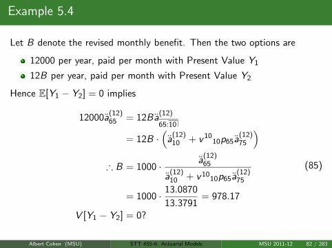
Let B denote the revised monthly benefit. Then the two options are
12000 per year, paid per month with Present Value Y1
12B per year, paid per month with Present Value Y2
Hence E[Y1 − Y2] = 0 implies
12000a(12)65 = 12Ba
(12)
65:10
= 12B ·(
a(12)10 + v 10
10p65a(12)75
)∴ B = 1000 ·
a(12)65
a(12)10 + v 10
10p65a(12)75
= 1000 · 13.0870
13.3791= 978.17
V [Y1 − Y2] = 0?
(85)
Albert Cohen (MSU) STT 455-6: Actuarial Models MSU 2011-12 82 / 283
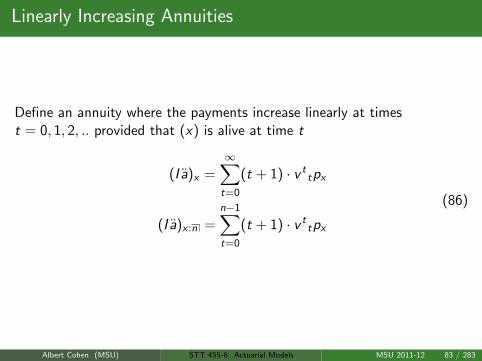
Linearly Increasing Annuities
Define an annuity where the payments increase linearly at timest = 0, 1, 2, .. provided that (x) is alive at time t
(I a)x =∞∑t=0
(t + 1) · v ttpx
(I a)x :n =n−1∑t=0
(t + 1) · v ttpx
(86)
Albert Cohen (MSU) STT 455-6: Actuarial Models MSU 2011-12 83 / 283
Linearly Increasing Annuities
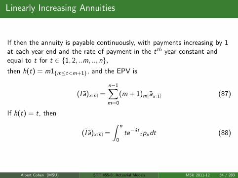
If then the annuity is payable continuously, with payments increasing by 1at each year end and the rate of payment in the tth year constant andequal to t for t ∈ 1, 2, ..m, .., n,then h(t) = m1m≤t<m+1, and the EPV is
(I a)x :n =n−1∑m=0
(m + 1)m|ax :1 (87)
If h(t) = t, then
(I a)x :n =
∫ n
0te−δt tpxdt (88)
Albert Cohen (MSU) STT 455-6: Actuarial Models MSU 2011-12 84 / 283
Evaluating Annuities Using Recursion
By recursion, we observe
ax = 1 + vpx + v 22px + v 3
3px + ....
= 1 + vpx
(1 + vpx+1 + v 2
2px+1 + v 33px+1 + ....
)= 1 + vpx ax+1
a(m)x =
1
m+ v
1m 1
mpx a
(m)
x+ 1m
(89)
Consider the case where there is a maximum age in the model, and so
aω−1 = 1
a(m)
ω− 1m
=1
m
(90)
Albert Cohen (MSU) STT 455-6: Actuarial Models MSU 2011-12 85 / 283
Evaluating Annuities Using Recursion
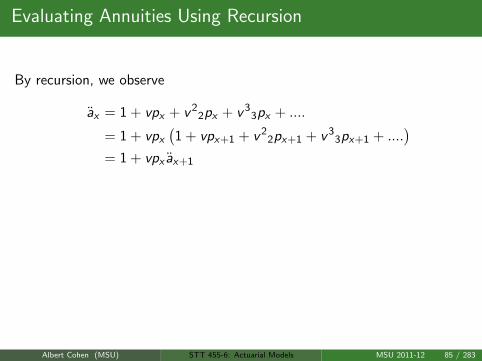
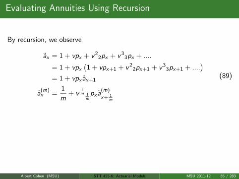
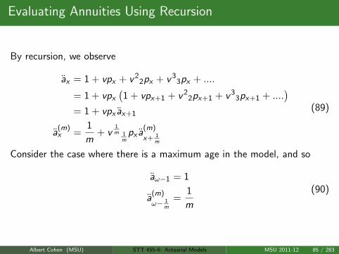
By recursion, we observe
ax = 1 + vpx + v 22px + v 3
3px + ....
= 1 + vpx
(1 + vpx+1 + v 2
2px+1 + v 33px+1 + ....
)= 1 + vpx ax+1
a(m)x =
1
m+ v
1m 1
mpx a
(m)
x+ 1m
(89)
Consider the case where there is a maximum age in the model, and so
aω−1 = 1
a(m)
ω− 1m
=1
m
(90)
Albert Cohen (MSU) STT 455-6: Actuarial Models MSU 2011-12 85 / 283
Evaluating Annuities Using UDD
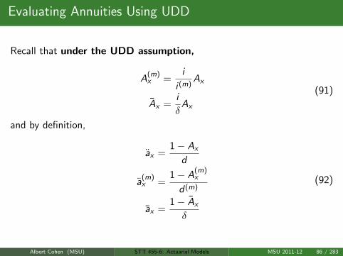
Recall that under the UDD assumption,
A(m)x =
i
i (m)Ax
Ax =i
δAx
(91)
and by definition,
ax =1− Ax
d
a(m)x =
1− A(m)x
d (m)
ax =1− Ax
δ
(92)
Albert Cohen (MSU) STT 455-6: Actuarial Models MSU 2011-12 86 / 283
Evaluating Annuities Using UDD
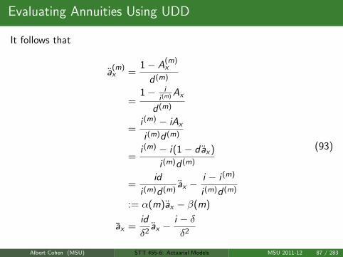
It follows that
a(m)x =
1− A(m)x
d (m)
=1− i
i (m) Ax
d (m)
=i (m) − iAx
i (m)d (m)
=i (m) − i(1− dax)
i (m)d (m)
=id
i (m)d (m)ax −
i − i (m)
i (m)d (m)
:= α(m)ax − β(m)
ax =id
δ2ax −
i − δδ2
(93)
Albert Cohen (MSU) STT 455-6: Actuarial Models MSU 2011-12 87 / 283
Evaluating Annuities Using UDD
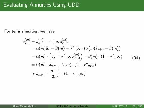
For term annuities, we have
a(m)x :n = a
(m)x − vn
npx a(m)x+n
= α(m)ax − β(m)− vnnpx · (α(m)ax+n − β(m))
= α(m) ·(
ax − vnnpx a
(m)x+n
)− β(m) · (1− vn
npx)
= α(m) · ax :n − β(m) · (1− vnnpx)
≈ ax :n −m − 1
2m· (1− vn
npx)
(94)
Albert Cohen (MSU) STT 455-6: Actuarial Models MSU 2011-12 88 / 283
Woolhouse’s Formula
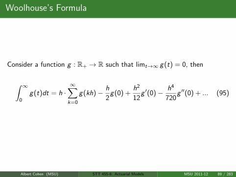
Consider a function g : R+ → R such that limt→∞ g(t) = 0, then
∫ ∞0
g(t)dt = h ·∞∑k=0
g(kh)− h
2g(0) +
h2
12g ′(0)− h4
720g ′′(0) + ... (95)
Albert Cohen (MSU) STT 455-6: Actuarial Models MSU 2011-12 89 / 283
Woolhouse’s Formula
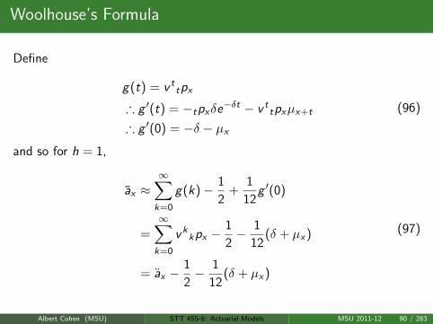
Define
g(t) = v ttpx
∴ g ′(t) = −tpxδe−δt − v ttpxµx+t
∴ g ′(0) = −δ − µx
(96)
and so for h = 1,
ax ≈∞∑k=0
g(k)− 1
2+
1
12g ′(0)
=∞∑k=0
vkkpx −
1
2− 1
12(δ + µx)
= ax −1
2− 1
12(δ + µx)
(97)
Albert Cohen (MSU) STT 455-6: Actuarial Models MSU 2011-12 90 / 283
Woolhouse’s Formula
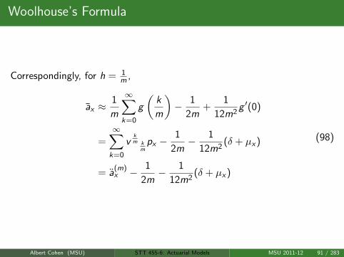
Correspondingly, for h = 1m ,
ax ≈1
m
∞∑k=0
g
(k
m
)− 1
2m+
1
12m2g ′(0)
=∞∑k=0
vkm k
mpx −
1
2m− 1
12m2(δ + µx)
= a(m)x − 1
2m− 1
12m2(δ + µx)
(98)
Albert Cohen (MSU) STT 455-6: Actuarial Models MSU 2011-12 91 / 283
Woolhouse’s Formula
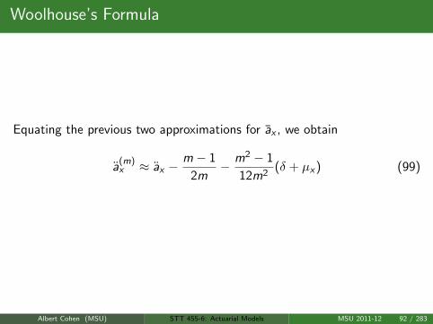
Equating the previous two approximations for ax , we obtain
a(m)x ≈ ax −
m − 1
2m− m2 − 1
12m2(δ + µx) (99)
Albert Cohen (MSU) STT 455-6: Actuarial Models MSU 2011-12 92 / 283
Woolhouse’s Formula
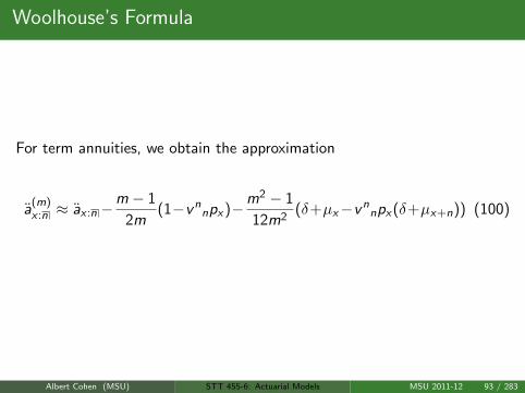
For term annuities, we obtain the approximation
a(m)x :n ≈ ax :n −
m − 1
2m(1−vn
npx)−m2 − 1
12m2(δ+µx−vn
npx(δ+µx+n)) (100)
Albert Cohen (MSU) STT 455-6: Actuarial Models MSU 2011-12 93 / 283
Woolhouse’s Formula
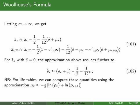
Letting m→∞, we get
ax ≈ ax −1
2− 1
12(δ + µx)
ax :n ≈ ax :n −1
2(1− vn
npx)− 1
12(δ + µx − vn
npx(δ + µx+n))
(101)
For ax with δ = 0, the approximation above reduces further to
ex ≈ (ex + 1)− 1
2− 1
12µx (102)
NB: For life tables, we can compute these quantities using theapproximation µx ≈ −1
2 [ln (px) + ln (px+1)]
Albert Cohen (MSU) STT 455-6: Actuarial Models MSU 2011-12 94 / 283

Select and Ultimate Survival Models
Notation:
Aggregate Survival Models: Models for a large population, where
tpx depends only on the current age x .
Select (and Ultimate) Survival Models: Models for a select groupof individuals that depend on the current age x and
Future survival probabilities for an individual in the group depend onthe individual’s current age and on the age at which the individualjoined the group∃d > 0 such that if an individual joined the group more than d yearsago, future survival probabilities depend only on current age. So, afterd years, the person is considered to be back in the aggregatepopulation.
Ultimately, a select survival model includes another event upon whichprobabilities are conditional on.
Albert Cohen (MSU) STT 455-6: Actuarial Models MSU 2011-12 95 / 283

Select and Ultimate Survival Models
Notation:
d is the select period
The mortality applicable to lives after the select period is over isknown as the ultimate mortality.
A select group should have a different mortality rate, as they have beenoffered (selected for) life insurance. A question, of course, is the effect onmortality by maintaining proper health insurance.
Albert Cohen (MSU) STT 455-6: Actuarial Models MSU 2011-12 96 / 283
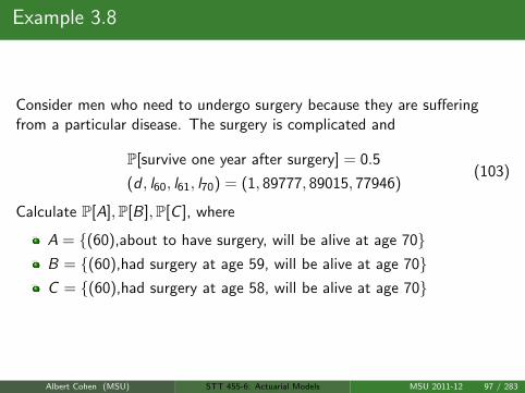
Example 3.8
Consider men who need to undergo surgery because they are sufferingfrom a particular disease. The surgery is complicated and
P[survive one year after surgery] = 0.5
(d , l60, l61, l70) = (1, 89777, 89015, 77946)(103)
Calculate P[A],P[B],P[C ], where
A = (60),about to have surgery, will be alive at age 70B = (60),had surgery at age 59, will be alive at age 70C = (60),had surgery at age 58, will be alive at age 70
Albert Cohen (MSU) STT 455-6: Actuarial Models MSU 2011-12 97 / 283
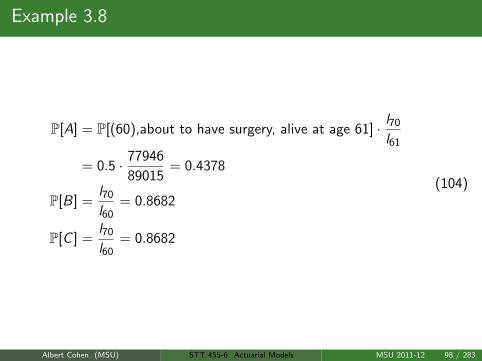
Example 3.8
P[A] = P[(60),about to have surgery, alive at age 61] · l70
l61
= 0.5 · 77946
89015= 0.4378
P[B] =l70
l60= 0.8682
P[C ] =l70
l60= 0.8682
(104)
Albert Cohen (MSU) STT 455-6: Actuarial Models MSU 2011-12 98 / 283
Select Survival Models
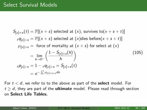
S[x]+s(t) = P[(x + s) selected at (x), survives to(x + s + t)]
tq[x]+s = P[(x + s) selected at (x)dies before(x + s + t)]
µ[x]+s = force of mortality at (x + s) for select at (x)
= limh→0+
(1− S[x]+s(h)
h
)tp[x]+s = 1− tq[x]+s = S[x]+s(t)
= e−∫ t
0 µ[x]+s+udu
(105)
For t < d , we refer to to the above as part of the select model. Fort ≥ d , they are part of the ultimate model. Please read through sectionon Select Life Tables.
Albert Cohen (MSU) STT 455-6: Actuarial Models MSU 2011-12 99 / 283

Select Life Tables
Sometimes, we wish to compute values from life tables. Consider again amodel where x ≥ x0, where x0 is the initial age, and 0 ≤ t ≤ d . Then
lx+d = d−tp[x]+t · l[x]+t (106)
Albert Cohen (MSU) STT 455-6: Actuarial Models MSU 2011-12 100 / 283
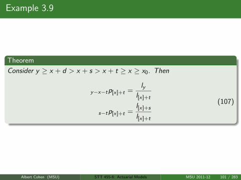
Example 3.9
Theorem
Consider y ≥ x + d > x + s > x + t ≥ x ≥ x0. Then
y−x−tp[x]+t =ly
l[x]+t
s−tp[x]+t =l[x]+s
l[x]+t
(107)
Albert Cohen (MSU) STT 455-6: Actuarial Models MSU 2011-12 101 / 283
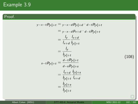
Example 3.9
Proof.
y−x−tp[x]+t = y−x−dp[x]+d · d−tp[x]+t
= y−x−dpx+d · d−tp[x]+t
=ly
lx+d
lx+d
l[x]+t
=ly
l[x]+t
s−tp[x]+t =d−tp[x]+t
d−sp[x]+s
=lx+d
l[x]+t
l[x]+s
lx+d
=l[x]+s
l[x]+t
(108)
Albert Cohen (MSU) STT 455-6: Actuarial Models MSU 2011-12 102 / 283
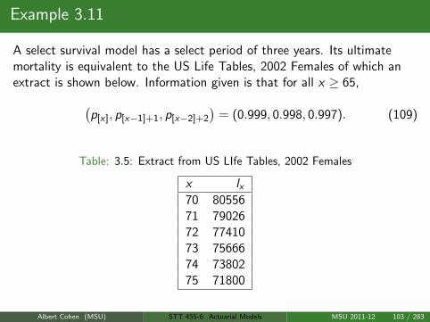
Example 3.11
A select survival model has a select period of three years. Its ultimatemortality is equivalent to the US Life Tables, 2002 Females of which anextract is shown below. Information given is that for all x ≥ 65,(
p[x], p[x−1]+1, p[x−2]+2
)= (0.999, 0.998, 0.997). (109)
Table: 3.5: Extract from US LIfe Tables, 2002 Females
x lx70 8055671 7902672 7741073 7566674 7380275 71800
Albert Cohen (MSU) STT 455-6: Actuarial Models MSU 2011-12 103 / 283

Example 3.11
Calculate the probability that a woman currently aged 70 will survive toage 75 given that
1 she was select at age 67:
2 she was select at age 68
3 she was select at age 69
4 she was select at age 70
Albert Cohen (MSU) STT 455-6: Actuarial Models MSU 2011-12 104 / 283
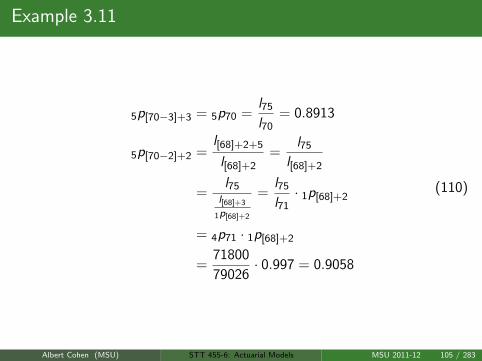
Example 3.11
5p[70−3]+3 = 5p70 =l75
l70= 0.8913
5p[70−2]+2 =l[68]+2+5
l[68]+2=
l75
l[68]+2
=l75
l[68]+3
1p[68]+2
=l75
l71· 1p[68]+2
= 4p71 · 1p[68]+2
=71800
79026· 0.997 = 0.9058
(110)
Albert Cohen (MSU) STT 455-6: Actuarial Models MSU 2011-12 105 / 283
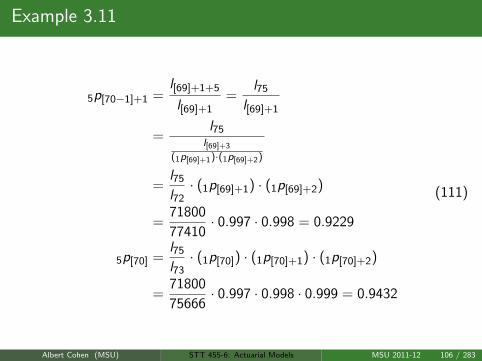
Example 3.11
5p[70−1]+1 =l[69]+1+5
l[69]+1=
l75
l[69]+1
=l75
l[69]+3
(1p[69]+1)·(1p[69]+2)
=l75
l72· (1p[69]+1) · (1p[69]+2)
=71800
77410· 0.997 · 0.998 = 0.9229
5p[70] =l75
l73· (1p[70]) · (1p[70]+1) · (1p[70]+2)
=71800
75666· 0.997 · 0.998 · 0.999 = 0.9432
(111)
Albert Cohen (MSU) STT 455-6: Actuarial Models MSU 2011-12 106 / 283

Example 3.12
Given a table of values for q[x], q[x−1]+1, qx and the knowledge that themodel incorporates a 2−year selct period, compute
4p[70]
3q[60]+1
4p[70] = p[70]p[70]+1p[70]+2p[70]+3 = p[70]p[70]+1p72p73
=(1− q[70]
)·(1− q[70]+1
)· (1− q72) · (1− q73)
3q[60]+1 = q[60]+1 + p[60]+1q62 + p[60]+1p62q63
= q[60]+1 +(1− q[60]+1
)· q62
+(1− q[60]+1
)· (1− q62) · q63
(112)
Albert Cohen (MSU) STT 455-6: Actuarial Models MSU 2011-12 107 / 283
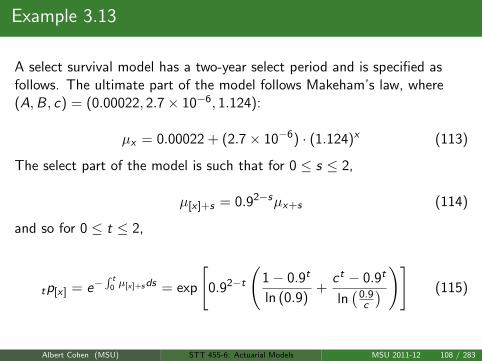
Example 3.13
A select survival model has a two-year select period and is specified asfollows. The ultimate part of the model follows Makeham’s law, where(A,B, c) = (0.00022, 2.7× 10⁻⁶, 1.124):
µx = 0.00022 + (2.7× 10−6) · (1.124)x (113)
The select part of the model is such that for 0 ≤ s ≤ 2,
µ[x]+s = 0.92−sµx+s (114)
and so for 0 ≤ t ≤ 2,
tp[x] = e−∫ t
0 µ[x]+sds = exp
[0.92−t
(1− 0.9t
ln (0.9)+
ct − 0.9t
ln(
0.9c
) )] (115)
Albert Cohen (MSU) STT 455-6: Actuarial Models MSU 2011-12 108 / 283

Example 3.13
It follows that given an initial cohort at age x0, that is given lx0 , we cancompute the entries of a select life table via
lx = px−1lx−1
l[x]+1 =lx+2
p[x]+1
l[x] =lx+2
2p[x]
(116)
Albert Cohen (MSU) STT 455-6: Actuarial Models MSU 2011-12 109 / 283

Homework Questions
HW: 3.1, 3.2, 3.4, 3.7, 3.8, 3.9, 3.10, 5.1, 5.3, 5.5, 5.6, 5.11, 5.14
Albert Cohen (MSU) STT 455-6: Actuarial Models MSU 2011-12 110 / 283

What is a Premium?
When entering into a contract, the financial obligations of all parties mustbe specified. In an insurance contract, the insurance company agrees topay the policyholder benefits in return for premium payments. Thepremiums secure the benefits as well as pay the company for expensesattached to the administation of the policy
Albert Cohen (MSU) STT 455-6: Actuarial Models MSU 2011-12 111 / 283

Premium Types
A Net Premium does not explicitly allow for company’s expenses, while aOffice or Gross Premium does. There may be a Single Premium or or aseries of payments that could even match with the policyholder’s salaryfreequency.
It is important to note that premiums are paid as soon as the contract issigned, otherwise the policyholder would attain coverage before paying forit with the first premium. This could be seen as an arbitrage opportunity -non-zero probability of gain with no money up front.
Albert Cohen (MSU) STT 455-6: Actuarial Models MSU 2011-12 112 / 283

Premium Types
Premiums cease upon death of the policyholder. The premium payingterm is the maximum length of time that premiums are required.Certainly, premium term can be fixed so that upon retirement, say, nomore payments are required.
Also, the benefits can be secured in the future (deferred) by a singlepremium payment up front. For example, pay now to secure annuitypayments upon retirement until death.
Albert Cohen (MSU) STT 455-6: Actuarial Models MSU 2011-12 113 / 283
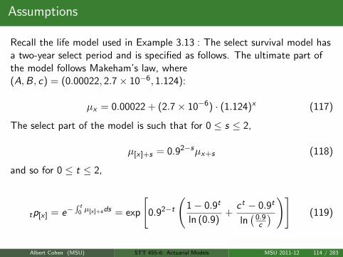
Assumptions
Recall the life model used in Example 3.13 : The select survival model hasa two-year select period and is specified as follows. The ultimate part ofthe model follows Makeham’s law, where(A,B, c) = (0.00022, 2.7× 10⁻⁶, 1.124):
µx = 0.00022 + (2.7× 10−6) · (1.124)x (117)
The select part of the model is such that for 0 ≤ s ≤ 2,
µ[x]+s = 0.92−sµx+s (118)
and so for 0 ≤ t ≤ 2,
tp[x] = e−∫ t
0 µ[x]+sds = exp
[0.92−t
(1− 0.9t
ln (0.9)+
ct − 0.9t
ln(
0.9c
) )] (119)
Albert Cohen (MSU) STT 455-6: Actuarial Models MSU 2011-12 114 / 283
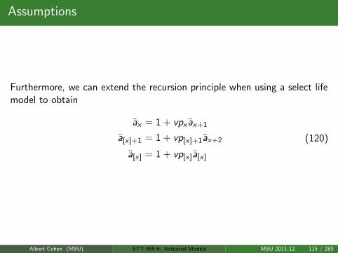
Assumptions
Furthermore, we can extend the recursion principle when using a select lifemodel to obtain
ax = 1 + vpx ax+1
a[x]+1 = 1 + vp[x]+1ax+2
a[x] = 1 + vp[x]a[x]
(120)
Albert Cohen (MSU) STT 455-6: Actuarial Models MSU 2011-12 115 / 283

Basic Model
In general, an insurance company can expect to have a total benefit paidout, along with expense loading and other related costs. We represent thistotal benefit as Z . Similarly, to fund Z , the company can expect thepolicyholder to make a single payment, or stream of payments, that haspresent value P · Y . Here, P represents the level premium P and Yrepresents the present value associated to a unit payment or paymentstream.
Albert Cohen (MSU) STT 455-6: Actuarial Models MSU 2011-12 116 / 283
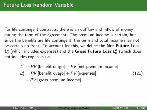
Future Loss Random Variable
For life contingent contracts, there is an outflow and inflow of moneyduring the term of the agreement. The premium income is certain, butsince the benefits are life contingent, the term and total income may notbe certain up front. To account for this, we define the Net Future LossLn
0 (which includes expenses) and the Gross Future Loss Lg0 (which does
not includes expenses) as
Ln0 = PV [benefit outgo]− PV [net premium income]
Lg0 = PV [benefit outgo] + PV [expenses]
− PV [gross premium income]
(121)
Albert Cohen (MSU) STT 455-6: Actuarial Models MSU 2011-12 117 / 283

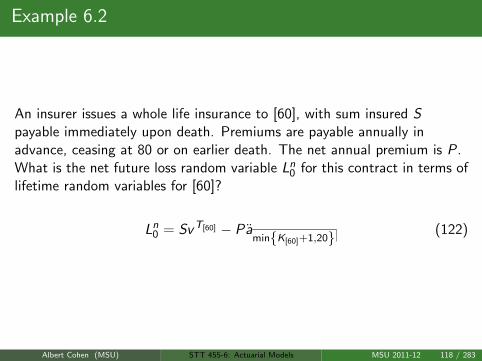
Example 6.2
An insurer issues a whole life insurance to [60], with sum insured Spayable immediately upon death. Premiums are payable annually inadvance, ceasing at 80 or on earlier death. The net annual premium is P.What is the net future loss random variable Ln
0 for this contract in terms oflifetime random variables for [60]?
Ln0 = SvT[60] − Pa
minK[60]+1,20 (122)
Albert Cohen (MSU) STT 455-6: Actuarial Models MSU 2011-12 118 / 283
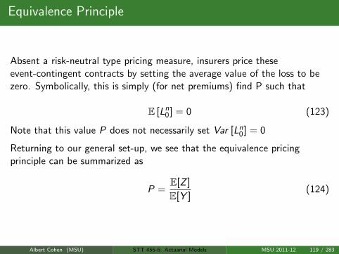
Equivalence Principle
Absent a risk-neutral type pricing measure, insurers price theseevent-contingent contracts by setting the average value of the loss to bezero. Symbolically, this is simply (for net premiums) find P such that
E [Ln0] = 0 (123)
Note that this value P does not necessarily set Var [Ln0] = 0
Returning to our general set-up, we see that the equivalence pricingprinciple can be summarized as
P =E[Z ]
E[Y ](124)
Albert Cohen (MSU) STT 455-6: Actuarial Models MSU 2011-12 119 / 283
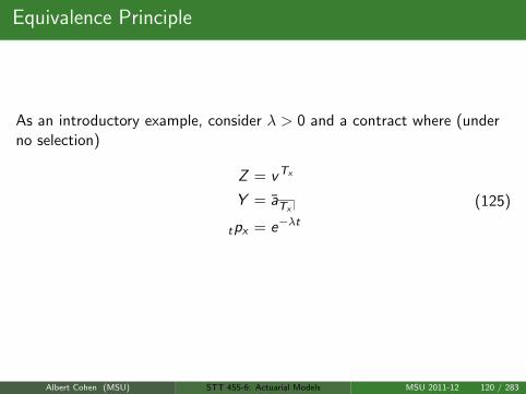
Equivalence Principle
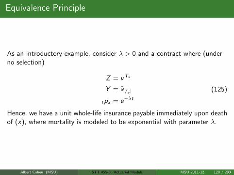
As an introductory example, consider λ > 0 and a contract where (underno selection)
Z = vTx
Y = aTx
tpx = e−λt(125)
Hence, we have a unit whole-life insurance payable immediately upon deathof (x), where mortality is modeled to be exponential with parameter λ.
Albert Cohen (MSU) STT 455-6: Actuarial Models MSU 2011-12 120 / 283
Equivalence Principle
As an introductory example, consider λ > 0 and a contract where (underno selection)
Z = vTx
Y = aTx
tpx = e−λt(125)
Hence, we have a unit whole-life insurance payable immediately upon deathof (x), where mortality is modeled to be exponential with parameter λ.
Albert Cohen (MSU) STT 455-6: Actuarial Models MSU 2011-12 120 / 283

Equivalence Principle
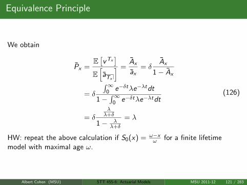
We obtain
Px =E[vTx]
E[aTx
] =Ax
ax= δ
Ax
1− Ax
= δ
∫∞0 e−δtλe−λtdt
1−∫∞
0 e−δtλe−λtdt
= δλλ+δ
1− λλ+δ
= λ
(126)
HW: repeat the above calculation if S0(x) = ω−xω for a finite lifetime
model with maximal age ω.
Albert Cohen (MSU) STT 455-6: Actuarial Models MSU 2011-12 121 / 283
Equivalence Principle
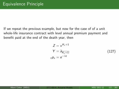
If we repeat the previous example, but now for the case of of a unitwhole-life insurance contract with level annual premium payment andbenefit paid at the end of the death year, then
Z = vKx+1
Y = aKx+1
tpx = e−λt(127)
Albert Cohen (MSU) STT 455-6: Actuarial Models MSU 2011-12 122 / 283

Equivalence Principle
It follows that
Px = dAx
1− Ax= d
∑∞k=0 e−δ(k+1) · (kpx − k+1px)
1−∑∞
k=0 e−δ(k+1) · (kpx − k+1px)
= d(1− e−λ) ·
∑∞k=0 e−δ(k+1)e−λk
1− (1− e−λ) ·∑∞
k=0 e−δte−λk
= d(1− e−λ) · e−δ · 1
1−e−(δ+λ)
1− (1− e−λ) · e−δ · 11−e−(δ+λ)
= (1− e−λ) · e−δ
(128)
Albert Cohen (MSU) STT 455-6: Actuarial Models MSU 2011-12 123 / 283
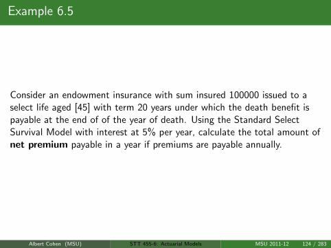
Example 6.5
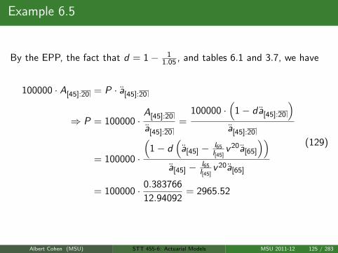
Consider an endowment insurance with sum insured 100000 issued to aselect life aged [45] with term 20 years under which the death benefit ispayable at the end of of the year of death. Using the Standard SelectSurvival Model with interest at 5% per year, calculate the total amount ofnet premium payable in a year if premiums are payable annually.
Albert Cohen (MSU) STT 455-6: Actuarial Models MSU 2011-12 124 / 283
Example 6.5
By the EPP, the fact that d = 1− 11.05 , and tables 6.1 and 3.7, we have
100000 · A[45]:20 = P · a[45]:20
⇒ P = 100000 ·A[45]:20
a[45]:20
=100000 ·
(1− da[45]:20
)a[45]:20
= 100000 ·
(1− d
(a[45] − l65
l[45]v 20a[65]
))a[45] − l65
l[45]v 20a[65]
= 100000 · 0.383766
12.94092= 2965.52
(129)
Albert Cohen (MSU) STT 455-6: Actuarial Models MSU 2011-12 125 / 283

New Business Strain
Starting up an insurance company requires start-up capital like most othercompanies. Agents are charged with drumming up new business in theform of finding and issuing new life insurance contracts. This helps todiversify risk in the case of a large loss on one contract (more on thislater.)
However, new contracts can incur larger losses up front in the first fewyears even without a benefit payout. This is due to initial commisionpayments to agents as well as contract preparation costs. Periodicmaintenance costs can also factor into the premium calculation.
Albert Cohen (MSU) STT 455-6: Actuarial Models MSU 2011-12 126 / 283

An Example..
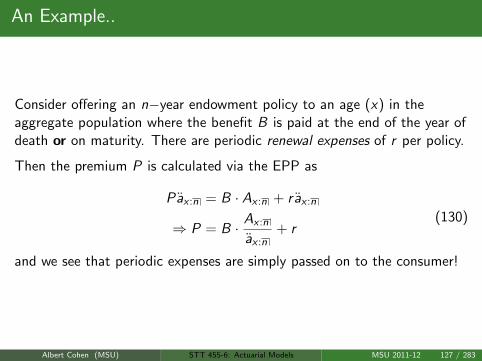
Consider offering an n−year endowment policy to an age (x) in theaggregate population where the benefit B is paid at the end of the year ofdeath or on maturity. There are periodic renewal expenses of r per policy.
Then the premium P is calculated via the EPP as
Pax :n = B · Ax :n + r ax :n
⇒ P = B · Ax :n
ax :n+ r
(130)
and we see that periodic expenses are simply passed on to the consumer!
Albert Cohen (MSU) STT 455-6: Actuarial Models MSU 2011-12 127 / 283
An Example..
Consider offering an n−year endowment policy to an age (x) in theaggregate population where the benefit B is paid at the end of the year ofdeath or on maturity. There are periodic renewal expenses of r per policy.
Then the premium P is calculated via the EPP as
Pax :n = B · Ax :n + r ax :n
⇒ P = B · Ax :n
ax :n+ r
(130)
and we see that periodic expenses are simply passed on to the consumer!
Albert Cohen (MSU) STT 455-6: Actuarial Models MSU 2011-12 127 / 283

Another Example..
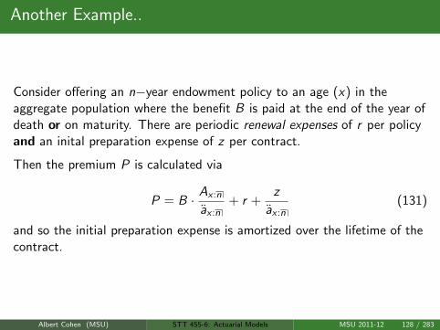
Consider offering an n−year endowment policy to an age (x) in theaggregate population where the benefit B is paid at the end of the year ofdeath or on maturity. There are periodic renewal expenses of r per policyand an inital preparation expense of z per contract.
Then the premium P is calculated via
P = B · Ax :n
ax :n+ r +
z
ax :n(131)
and so the initial preparation expense is amortized over the lifetime of thecontract.
Albert Cohen (MSU) STT 455-6: Actuarial Models MSU 2011-12 128 / 283
Another Example..
Consider offering an n−year endowment policy to an age (x) in theaggregate population where the benefit B is paid at the end of the year ofdeath or on maturity. There are periodic renewal expenses of r per policyand an inital preparation expense of z per contract.
Then the premium P is calculated via
P = B · Ax :n
ax :n+ r +
z
ax :n(131)
and so the initial preparation expense is amortized over the lifetime of thecontract.
Albert Cohen (MSU) STT 455-6: Actuarial Models MSU 2011-12 128 / 283

Example 6.6
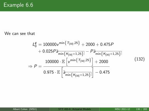
An insurer issues a 25−year annual premium endowment insurance withsum insured 100000 to a select life aged [30]. The insurer incurs initialexpenses of 2000 plus 50% of the first premium and renewable expenses of2.5% of each subsequent premium. The death benefit is payableimmediately upon death. What is the annual premium P?
Albert Cohen (MSU) STT 455-6: Actuarial Models MSU 2011-12 129 / 283
Example 6.6
We can see that
Lg0 = 100000v minT[30],25 + 2000 + 0.475P
+ 0.025PaminK[30]+1,25 − Pa
minK[30]+1,25
⇒ P =100000 · E
[v minT[30],25
]+ 2000
0.975 · E[
aminK[30]+1,25
]− 0.475
(132)
Albert Cohen (MSU) STT 455-6: Actuarial Models MSU 2011-12 130 / 283
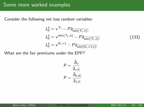
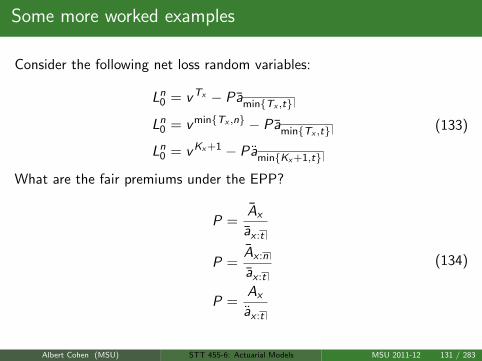
Some more worked examples
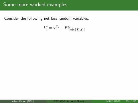
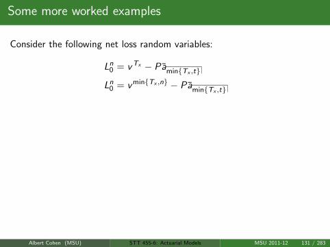
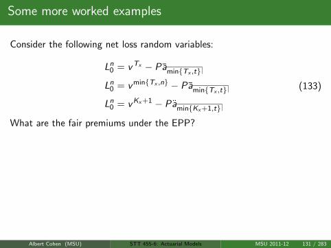
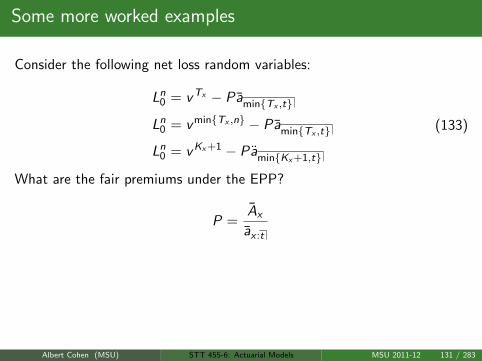
Consider the following net loss random variables:
Ln0 = vTx − PaminTx ,t
Ln0 = v minTx ,n − PaminTx ,t
Ln0 = vKx+1 − PaminKx+1,t
(133)
What are the fair premiums under the EPP?
P =Ax
ax :t
P =Ax :n
ax :t
P =Ax
ax :t
(134)
Albert Cohen (MSU) STT 455-6: Actuarial Models MSU 2011-12 131 / 283
Some more worked examples
Consider the following net loss random variables:
Ln0 = vTx − PaminTx ,t
Ln0 = v minTx ,n − PaminTx ,t
Ln0 = vKx+1 − PaminKx+1,t
(133)
What are the fair premiums under the EPP?
P =Ax
ax :t
P =Ax :n
ax :t
P =Ax
ax :t
(134)
Albert Cohen (MSU) STT 455-6: Actuarial Models MSU 2011-12 131 / 283
Refunded Deferred Annual Whole-Life Annuity Due
Consider the case where a n−year deferred annual whole-life annuity dueof 1 on a life (x) where if the death occurs during the deferral period, thesingle benefit premium is refunded without interest at the end of theyear of death. What is this single benefit premium P?
Albert Cohen (MSU) STT 455-6: Actuarial Models MSU 2011-12 132 / 283
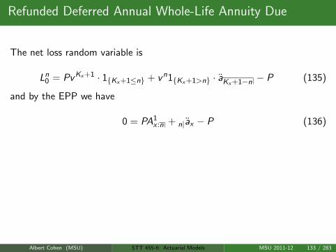
Refunded Deferred Annual Whole-Life Annuity Due
The net loss random variable is
Ln0 = PvKx+1 · 1Kx+1≤n + vn1Kx+1>n · aKx+1−n − P (135)
and by the EPP we have
0 = PA1x :n + n|ax − P (136)
This implies that
P =n|ax
1− A1x :n
=Ax :n − A1
x :n
1− A1x :n
· ax+n
(137)
Albert Cohen (MSU) STT 455-6: Actuarial Models MSU 2011-12 133 / 283
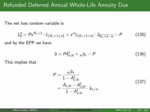
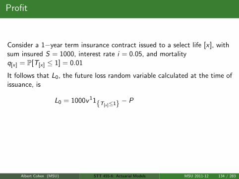
Profit
Consider a 1−year term insurance contract issued to a select life [x ], withsum insured S = 1000, interest rate i = 0.05, and mortalityq[x] = P[T[x] ≤ 1] = 0.01
It follows that L0, the future loss random variable calculated at the time ofissuance, is
L0 = 1000v 11T[x]≤1 − P
⇒ P = E[1000v 11T[x]≤1] = 1000v · P[T[x] ≤ 1]
=(1000)(0.01)
1.05= 9.52
(138)
Albert Cohen (MSU) STT 455-6: Actuarial Models MSU 2011-12 134 / 283
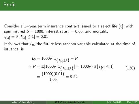

Profit
Consider that the company has issued a lot of these contracts, say N 1,to independent select lives [x ]. Let D[x] be the random variablerepresenting the number of deaths in a year of this population, and assume
D[x] ∼ Bin(N, q[x]) (139)
Albert Cohen (MSU) STT 455-6: Actuarial Models MSU 2011-12 135 / 283
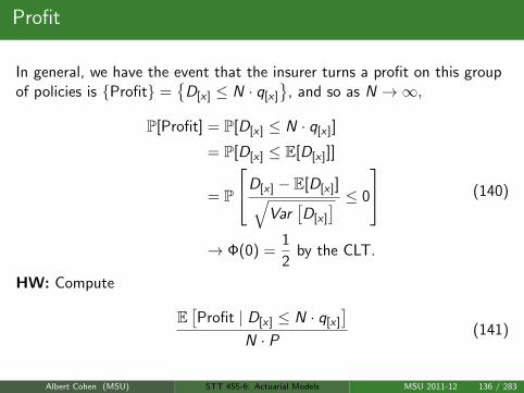
Profit
In general, we have the event that the insurer turns a profit on this groupof policies is Profit =
D[x] ≤ N · q[x]
, and so as N →∞,
P[Profit] = P[D[x] ≤ N · q[x]]
= P[D[x] ≤ E[D[x]]]
= P
D[x] − E[D[x]]√Var
[D[x]
] ≤ 0
→ Φ(0) =
1
2by the CLT.
(140)
HW: Compute
E[Profit | D[x] ≤ N · q[x]
]N · P
(141)
Albert Cohen (MSU) STT 455-6: Actuarial Models MSU 2011-12 136 / 283

Profit
Consider now a whole-life contract issued to [x ] with sum insured S andannual premium P. Then
P[Profit] = P[L0 < 0] = P[SvK[x]+1 − PaK[x]+1 < 0]
= P[SvK[x]+1 < P · 1− vK[x]+1
d]
= P[
vK[x]+1 <P
P + d · S
]= P
[K[x] + 1 >
1
δln
(P
P + d · S
)]= P
[K[x] + 1 > b1
δln
(P
P + d · S
)c]
= b 1δ
ln ( PP+d·S )cp[x]
(142)
Albert Cohen (MSU) STT 455-6: Actuarial Models MSU 2011-12 137 / 283
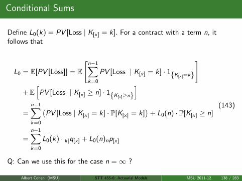
Conditional Sums
Define L0(k) = PV [Loss | K[x] = k]. For a contract with a term n, itfollows that
L0 = E[PV [Loss]] = E
[n−1∑k=0
PV [Loss | K[x] = k] · 1K[x]=k
]+ E
[PV [Loss | K[x] ≥ n] · 1K[x]≥n
]=
n−1∑k=0
(PV [Loss | K[x] = k] · P[K[x] = k]
)+ L0(n) · P[K[x] ≥ n]
=n−1∑k=0
L0(k) · k|q[x] + L0(n)np[x]
(143)
Q: Can we use this for the case n =∞ ?
Albert Cohen (MSU) STT 455-6: Actuarial Models MSU 2011-12 138 / 283
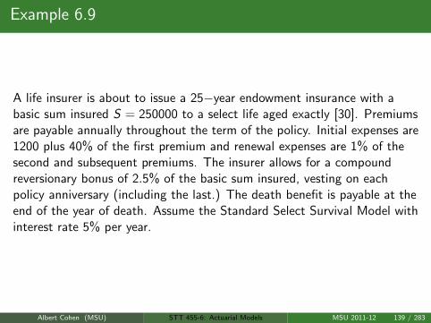
Example 6.9
A life insurer is about to issue a 25−year endowment insurance with abasic sum insured S = 250000 to a select life aged exactly [30]. Premiumsare payable annually throughout the term of the policy. Initial expenses are1200 plus 40% of the first premium and renewal expenses are 1% of thesecond and subsequent premiums. The insurer allows for a compoundreversionary bonus of 2.5% of the basic sum insured, vesting on eachpolicy anniversary (including the last.) The death benefit is payable at theend of the year of death. Assume the Standard Select Survival Model withinterest rate 5% per year.
Albert Cohen (MSU) STT 455-6: Actuarial Models MSU 2011-12 139 / 283
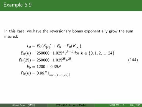
Example 6.9
In this case, we have the reversionary bonus exponentially grow the suminsured:
L0 = B0(K[x]) + E0 − P0(K[x])
B0(k) = 250000 · 1.025kvk+1 for k ∈ 0, 1, 2, ..., 24B0(25) = 250000 · 1.02525v 25
E0 = 1200 + 0.39P
P0(k) = 0.99Pamin k+1,25
(144)
Albert Cohen (MSU) STT 455-6: Actuarial Models MSU 2011-12 140 / 283
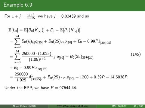
Example 6.9
For 1 + j = 1+i1.025 , we have j = 0.02439 and so
E[L0] = E[B0(K[x])] + E0 − E[P0(K[x])]
=24∑k=0
B0(k)k|q[30] + B0(25)25p[30] + E0 − 0.99Pa[30]:25
=24∑k=0
250000 · (1.025)t
(1.05)t+1 k|q[30] + B0(25)25p[30]
+ E0 − 0.99Pa[30]:25
=250000
1.025A1
[30]25 j+ B0(25) · 25p[30] + 1200 + 0.39P − 14.5838P
(145)
Under the EPP, we have P = 97644.44.
HW: Replicate Table 6.3 in the text by using a spreadsheet program.Compare this example with Example 6.10.
Albert Cohen (MSU) STT 455-6: Actuarial Models MSU 2011-12 141 / 283
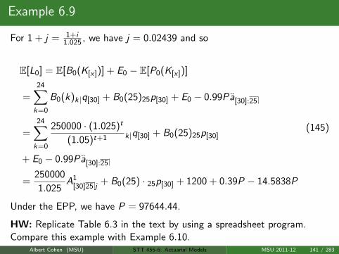
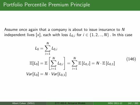
Portfolio Percentile Premium Principle
Assume once again that a company is about to issue insurance to Nindependent lives [x ], each with loss L0,i for i ∈ 1, 2, ..,N . In this case
L0 =N∑i=1
L0,i
E[L0] = E
[N∑i=1
L0,i
]=
N∑i=1
E [L0,i ] = N · E [L0,1]
Var [L0] = N · Var [L0,1]
(146)
Albert Cohen (MSU) STT 455-6: Actuarial Models MSU 2011-12 142 / 283
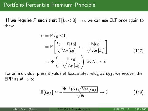
Portfolio Percentile Premium Principle
If we require P such that P[L0 < 0] = α, we can use CLT once again toshow
α = P[L0 < 0]
= P
[L0 − E[L0]√
Var [L0]< − E[L0]√
Var [L0]
]
→ Φ
(− E[L0]√
Var [L0]
)as N →∞
(147)
For an individual present value of loss, stated wlog as L0,1, we recover theEPP as N →∞
E[L0,1] ≈ −Φ−1(α)
√Var [L0,1]
√N
→ 0 (148)
Albert Cohen (MSU) STT 455-6: Actuarial Models MSU 2011-12 143 / 283
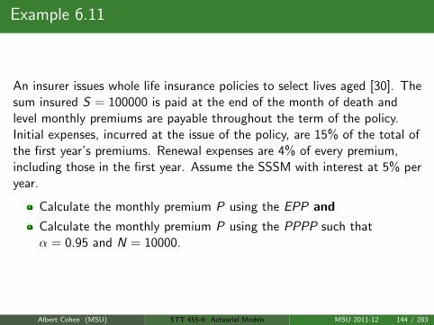
Example 6.11
An insurer issues whole life insurance policies to select lives aged [30]. Thesum insured S = 100000 is paid at the end of the month of death andlevel monthly premiums are payable throughout the term of the policy.Initial expenses, incurred at the issue of the policy, are 15% of the total ofthe first year’s premiums. Renewal expenses are 4% of every premium,including those in the first year. Assume the SSSM with interest at 5% peryear.
Calculate the monthly premium P using the EPP and
Calculate the monthly premium P using the PPPP such thatα = 0.95 and N = 10000.
Albert Cohen (MSU) STT 455-6: Actuarial Models MSU 2011-12 144 / 283
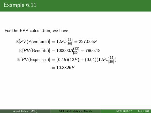
Example 6.11
For the EPP calculation, we have
E[PV (Premiums)] = 12Pa(12)[30] = 227.065P
E[PV (Benefits)] = 100000A(12)[30] = 7866.18
E[PV (Expenses)] = (0.15)(12P) + (0.04)(12Pa(12)[30] )
= 10.8826P
E[PV (Premiums)] = E[PV (Benefits)] + E[PV (Expenses)]
⇒ P = 36.39
(149)
Albert Cohen (MSU) STT 455-6: Actuarial Models MSU 2011-12 145 / 283
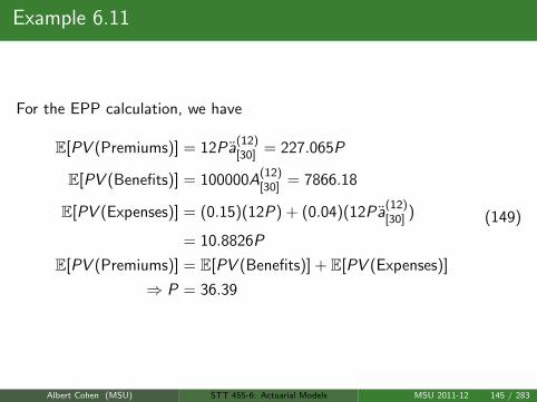
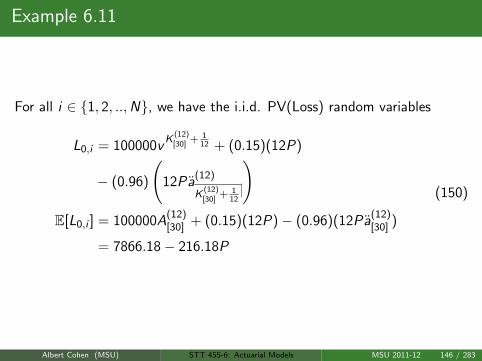
Example 6.11
For all i ∈ 1, 2, ..,N, we have the i.i.d. PV(Loss) random variables
L0,i = 100000vK
(12)[30]
+ 112 + (0.15)(12P)
− (0.96)
(12Pa
(12)
K(12)[30]
+ 112
)E[L0,i ] = 100000A
(12)[30] + (0.15)(12P)− (0.96)(12Pa
(12)[30] )
= 7866.18− 216.18P
(150)
Albert Cohen (MSU) STT 455-6: Actuarial Models MSU 2011-12 146 / 283
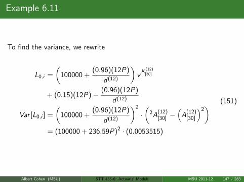
Example 6.11
To find the variance, we rewrite
L0,i =
(100000 +
(0.96)(12P)
d (12)
)vK
(12)[30]
+ (0.15)(12P)− (0.96)(12P)
d (12)
Var [L0,i ] =
(100000 +
(0.96)(12P)
d (12)
)2
·(
2A(12)[30] −
(A
(12)[30]
)2)
= (100000 + 236.59P)2 · (0.0053515)
(151)
Albert Cohen (MSU) STT 455-6: Actuarial Models MSU 2011-12 147 / 283
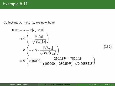
Example 6.11
Collecting our results, we now have
0.95 = α = P[L0 < 0]
≈ Φ
(− E[L0]√
Var [L0]
)
= Φ
(−√
N · E[L0,1]√Var [L0,1]
)
= Φ
(√10000 · 216.18P − 7866.18
(100000 + 236.59P) ·√
0.0053515
)(152)
Albert Cohen (MSU) STT 455-6: Actuarial Models MSU 2011-12 148 / 283
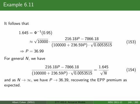
Example 6.11
It follows that
1.645 = Φ−1(0.95)
≈√
10000 · 216.18P − 7866.18
(100000 + 236.59P) ·√
0.0053515
⇒ P = 36.99
(153)
For general N, we have
216.18P − 7866.18
(100000 + 236.59P) ·√
0.0053515=
1.645√N
(154)
and as N →∞, we have P → 36.39, recovering the EPP premium asexpected.
Albert Cohen (MSU) STT 455-6: Actuarial Models MSU 2011-12 149 / 283
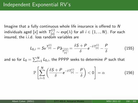
Independent Exponential RV’s
Imagine that a fully continuous whole life insurance is offered to N
individuals aged [x ] with T(i)[x] ∼ exp(λ) for all i ∈ 1, ..,N. For each
insured, the i.i.d. loss random variables are
L0,i = SvT
(i)[x] − Pa
T(i)[x]
=δS + P
δe−δT (i)
[x] − P
δ(155)
and so for L0 =∑N
i=1 L0,i , the PPPP seeks to determine P such that
P
[N∑i=1
(δS + P
δe−δT (i)
[x] − P
δ
)< 0
]= α (156)
Albert Cohen (MSU) STT 455-6: Actuarial Models MSU 2011-12 150 / 283
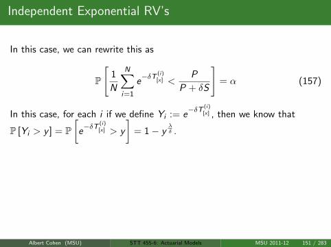
Independent Exponential RV’s
In this case, we can rewrite this as
P
[1
N
N∑i=1
e−δT (i)
[x] <P
P + δS
]= α (157)
In this case, for each i if we define Yi := e−δT (i)
[x] , then we know that
P [Yi > y ] = P[
e−δT (i)
[x] > y
]= 1− y
λδ .
HW Using convolution techniques, find the above probability
P
[1
N
N∑i=1
Yi <P
P + δS
]= α. (158)
Are there any ergodic theory results that we can use?
Albert Cohen (MSU) STT 455-6: Actuarial Models MSU 2011-12 151 / 283
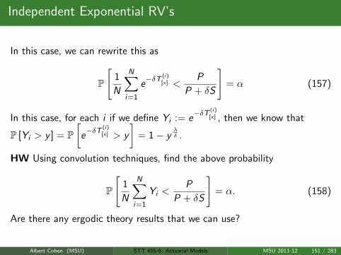
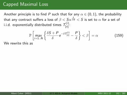
Capped Maximal Loss
Another principle is to find P such that for any α ∈ (0, 1), the probability
that any contract suffers a loss of β < SαδλN < S is set to α for a set of
i.i.d. exponentially distributed times T(i)[x] :
P[
maxi=1..N
δS + P
δe−δT (i)
[x] − P
δ
< β
]= α (159)
We rewrite this as
α = P[
mini=1..N
T
(i)[x]
> −1
δln
(P + δβ
P + δ
)]=(
e−λ[− 1δ
ln (P+δβP+δ )]
)N=
(P + δβ
P + δS
)λNδ
P = δ · SαδλN − β
1− αδλN
→∞ as N →∞
(160)
For this risk measure, is there a number of policy holders N that is toohigh?
Albert Cohen (MSU) STT 455-6: Actuarial Models MSU 2011-12 152 / 283
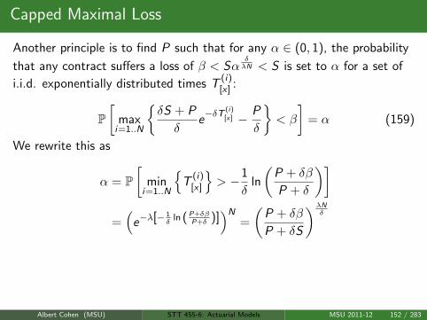
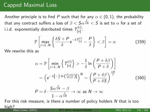
Comments on PPPP
Notice that the PPPP only guarantees that the probability of a loss is1− α.
It says nothing about the size of what that loss could be if itarises.
This is a big problem if the loss is extremely large and bankrupts theinsurer. It may seem very unlikely, but recent economic events haveshown otherwise.
Further improvements to this model can be seen in the ERM forStrategic Management (Status Report) by Gary Venter, posted onthe SOA.org website
Also, there is a close link, perhaps to be explored in a project, withVAR in the financial world. Click here for an informative article in theNY Times TM for an article on VAR and the recent financial crisis.
Albert Cohen (MSU) STT 455-6: Actuarial Models MSU 2011-12 153 / 283

Homework Questions
HW: 6.1, 6.2, 6.5, 6.7, 6.8, 6.12, 6.14, 6.15
Albert Cohen (MSU) STT 455-6: Actuarial Models MSU 2011-12 154 / 283
Policy Value Basis
When entering into a contract, the financial obligations of all partiesshould be specified at the time the agreement is signed. This includesdisclosure of health status, age, and premium payments expected to fundbenefits and expenses associated with the contract.The Policy Value tV is the expected value of the future loss randomvariable Lt at time t:
tV = E[Lt ] = E[ Loss | T[x] > t] (161)
Albert Cohen (MSU) STT 455-6: Actuarial Models MSU 2011-12 155 / 283
Policy Value Basis
Definition
The gross premium policy value for a policy in force at durationt ≥ 0 years after it was purchased is the expected value at that timeof the gross future loss random variable on a specified basis. Thepremiums used in the calculation are the actual premiums payableunder the contract.
The net premium policy value for a policy in force at durationt ≥ 0 years after it was purchased is the expected value at that timeof the net future loss random variable on a specified basis (whichmakes no allowance for expenses.) The premiums used in thecalculation are the net premiums calculated on the policy value basisusing the equivalence principle, not the actual premiums payable
It is important to note that usual practice dictates that when calculating
tV , premiums and premium-related expenses due at t are regarded asfuture payments and any insurance benefits and related expenses as pastpayments.
Albert Cohen (MSU) STT 455-6: Actuarial Models MSU 2011-12 156 / 283
Recursion
Define
Pt as the premium payable at time t
et as the premium-related expense payable at time t
St+1 as the sum insured payable at time t + 1
Et+1 as the expense of paying the sum insured at time t + 1
t+1V as the gross premium policy value for a policy in force at timet + 1
Lt as the gross future loss random variable at time t
it as the interest rate from time t to time t + 1.
Albert Cohen (MSU) STT 455-6: Actuarial Models MSU 2011-12 157 / 283
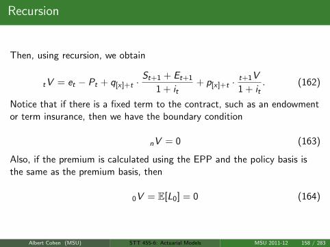
Recursion
Then, using recursion, we obtain
tV = et − Pt + q[x]+t ·St+1 + Et+1
1 + it+ p[x]+t ·
t+1V
1 + it. (162)
Notice that if there is a fixed term to the contract, such as an endowmentor term insurance, then we have the boundary condition
nV = 0 (163)
Also, if the premium is calculated using the EPP and the policy basis isthe same as the premium basis, then
0V = E[L0] = 0 (164)
Albert Cohen (MSU) STT 455-6: Actuarial Models MSU 2011-12 158 / 283
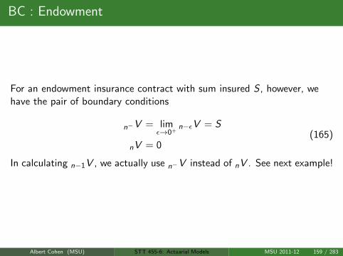
BC : Endowment
For an endowment insurance contract with sum insured S , however, wehave the pair of boundary conditions
n−V = limε→0+
n−εV = S
nV = 0(165)
In calculating n−1V , we actually use n−V instead of nV . See next example!
Albert Cohen (MSU) STT 455-6: Actuarial Models MSU 2011-12 159 / 283
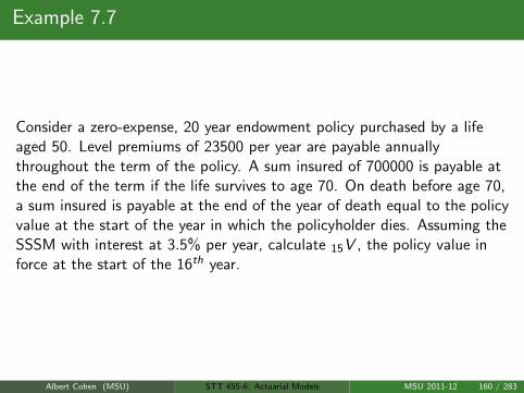
Example 7.7
Consider a zero-expense, 20 year endowment policy purchased by a lifeaged 50. Level premiums of 23500 per year are payable annuallythroughout the term of the policy. A sum insured of 700000 is payable atthe end of the term if the life survives to age 70. On death before age 70,a sum insured is payable at the end of the year of death equal to the policyvalue at the start of the year in which the policyholder dies. Assuming theSSSM with interest at 3.5% per year, calculate 15V , the policy value inforce at the start of the 16th year.
Albert Cohen (MSU) STT 455-6: Actuarial Models MSU 2011-12 160 / 283
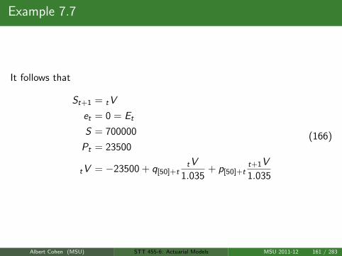
Example 7.7
It follows that
St+1 = tV
et = 0 = Et
S = 700000
Pt = 23500
tV = −23500 + q[50]+ttV
1.035+ p[50]+t
t+1V
1.035
(166)
Albert Cohen (MSU) STT 455-6: Actuarial Models MSU 2011-12 161 / 283

Example 7.7
Combining with our boundary value, we obtain the difference equation
tV =p[50]+t · t+1V − 24322.50
p[50]+t + 0.035
20−V = 700000.
(167)
Our initial iteration actually uses 20−V to obtain
19V =p69 · (20−V )− 24322.50
p69 + 0.035= 652401 (168)
Use tables or spreadsheet to calculate SSSM values and obtain
15V = 478063.
Albert Cohen (MSU) STT 455-6: Actuarial Models MSU 2011-12 162 / 283
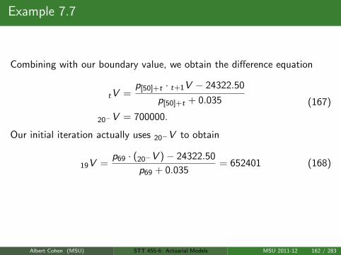
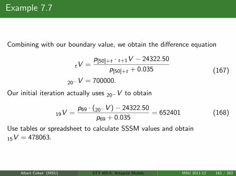

Example 7.1
Consider a 20−year endowment policy purchased by a life aged 50. Levelpremiums are payable annually throughout the term of the policy and thesum insured, S = 500000, is payable at the end of the year of death or atthe end of the term, whichever is sooner. The basis used by the insurancecompany for all calculations is under the SSSM with 5% per year interestand no allowance for expenses. Calculate P under the EPPP and thecorresponding policy values
Albert Cohen (MSU) STT 455-6: Actuarial Models MSU 2011-12 163 / 283
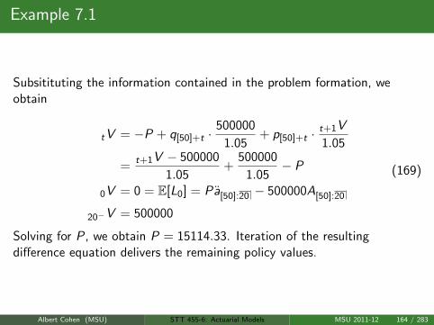
Example 7.1
Subsitituting the information contained in the problem formation, weobtain
tV = −P + q[50]+t ·500000
1.05+ p[50]+t ·
t+1V
1.05
=t+1V − 500000
1.05+
500000
1.05− P
0V = 0 = E[L0] = Pa[50]:20 − 500000A[50]:20
20−V = 500000
(169)
Solving for P, we obtain P = 15114.33. Iteration of the resultingdifference equation delivers the remaining policy values.
Albert Cohen (MSU) STT 455-6: Actuarial Models MSU 2011-12 164 / 283
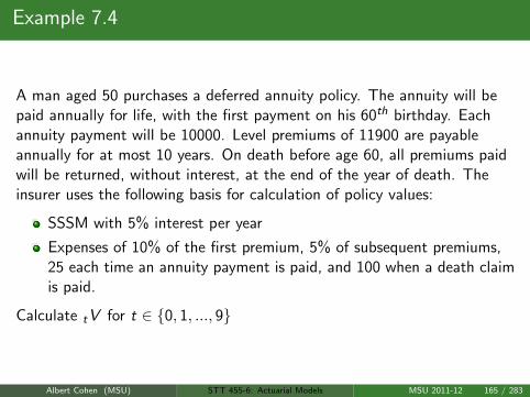
Example 7.4
A man aged 50 purchases a deferred annuity policy. The annuity will bepaid annually for life, with the first payment on his 60th birthday. Eachannuity payment will be 10000. Level premiums of 11900 are payableannually for at most 10 years. On death before age 60, all premiums paidwill be returned, without interest, at the end of the year of death. Theinsurer uses the following basis for calculation of policy values:
SSSM with 5% interest per year
Expenses of 10% of the first premium, 5% of subsequent premiums,25 each time an annuity payment is paid, and 100 when a death claimis paid.
Calculate tV for t ∈ 0, 1, ..., 9
Albert Cohen (MSU) STT 455-6: Actuarial Models MSU 2011-12 165 / 283
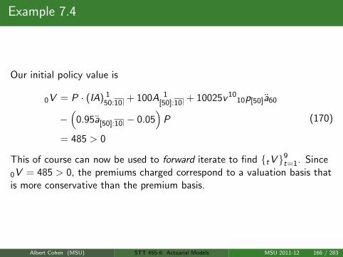
Example 7.4
Our initial policy value is
0V = P · (IA) 150:10
+ 100A 1[50]:10
+ 10025v 1010p[50]a60
−(
0.95a[50]:10 − 0.05)
P
= 485 > 0
(170)
This of course can now be used to forward iterate to find tV 9t=1. Since
0V = 485 > 0, the premiums charged correspond to a valuation basis thatis more conservative than the premium basis.
Albert Cohen (MSU) STT 455-6: Actuarial Models MSU 2011-12 166 / 283
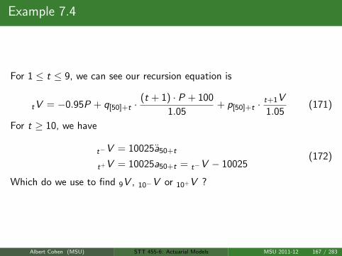
Example 7.4
For 1 ≤ t ≤ 9, we can see our recursion equation is
tV = −0.95P + q[50]+t ·(t + 1) · P + 100
1.05+ p[50]+t ·
t+1V
1.05(171)
For t ≥ 10, we have
t−V = 10025a50+t
t+V = 10025a50+t = t−V − 10025(172)
Which do we use to find 9V , 10−V or 10+V ?
Albert Cohen (MSU) STT 455-6: Actuarial Models MSU 2011-12 167 / 283
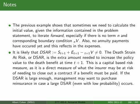
Notes
The previous example shows that sometimes we need to calculate theinitial value, given the information contained in the problemstatement, to iterate forward, especially if there is no term n andcorresponding boundary condition nV . Also, no annuity paymentshave occured yet and this reflects in the expenses.
It is likely that DSAR := St+1 + Et+1 − t+1V 6= 0. The Death StrainAt Risk, or DSAR, is the extra amount needed to increase the policyvalue to the death benefit at time t + 1. This is a capital based riskmeasure, as it is a direct measure of what the insurer may be at riskof needing to close out a contract if a benefit must be paid. If theDSAR is large enough, management may want to purchasereinsurance in case a large DSAR (even with low probability) occurs.
Albert Cohen (MSU) STT 455-6: Actuarial Models MSU 2011-12 168 / 283

Example 7.3
A woman aged 60 purchases a 20 year endowment insurance with a suminsured S = 100000 payable at the end of the year of death or on survivalto age 80, whichever occurs first. An annual premium of 5200 ispayable for at most 10 years. The insurer uses the following basis forcalculation of policy values:
SSSM with 5% interest per year
Expenses of 10% of the first premium, 5% of subsequent premiums,and 200 on payment of the sum insured.
Albert Cohen (MSU) STT 455-6: Actuarial Models MSU 2011-12 169 / 283
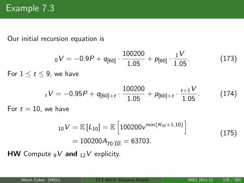
Example 7.3
Our initial recursion equation is
0V = −0.9P + q[60] ·100200
1.05+ p[60] ·
1V
1.05. (173)
For 1 ≤ t ≤ 9, we have
tV = −0.95P + q[60]+t ·100200
1.05+ p[60]+t ·
t+1V
1.05. (174)
For t = 10, we have
10V = E [L10] = E[100200v minK70+1,10
]= 100200A70:10 = 63703.
(175)
HW Compute 9V and 12V explicity.
Albert Cohen (MSU) STT 455-6: Actuarial Models MSU 2011-12 170 / 283
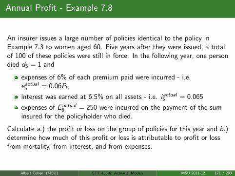
Annual Profit - Example 7.8
An insurer issues a large number of policies identical to the policy inExample 7.3 to women aged 60. Five years after they were issued, a totalof 100 of these policies were still in force. In the following year, one persondied d5 = 1 and
expenses of 6% of each premium paid were incurred - i.e.eactual5 = 0.06P5
interest was earned at 6.5% on all assets - i.e. iactual5 = 0.065
expenses of E actual6 = 250 were incurred on the payment of the sum
insured for the policyholder who died.
Calculate a.) the profit or loss on the group of policies for this year and b.)determine how much of this profit or loss is attributable to profit or lossfrom mortality, from interest, and from expenses.
Albert Cohen (MSU) STT 455-6: Actuarial Models MSU 2011-12 171 / 283
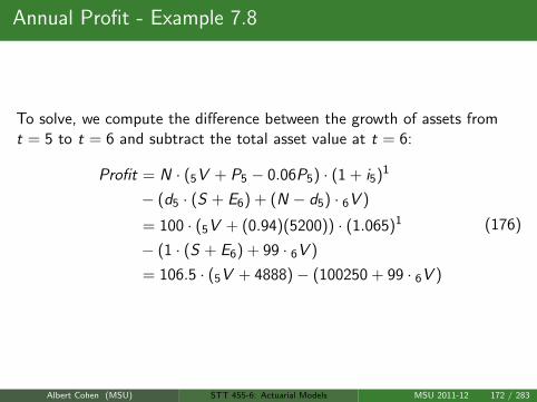
Annual Profit - Example 7.8
To solve, we compute the difference between the growth of assets fromt = 5 to t = 6 and subtract the total asset value at t = 6:
Profit = N · (5V + P5 − 0.06P5) · (1 + i5)1
− (d5 · (S + E6) + (N − d5) · 6V )
= 100 · (5V + (0.94)(5200)) · (1.065)1
− (1 · (S + E6) + 99 · 6V )
= 106.5 · (5V + 4888)− (100250 + 99 · 6V )
(176)
Albert Cohen (MSU) STT 455-6: Actuarial Models MSU 2011-12 172 / 283
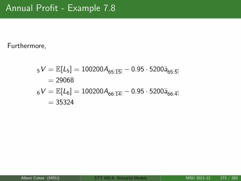
Annual Profit - Example 7.8
Furthermore,
5V = E[L5] = 100200A65:15 − 0.95 · 5200a65:5
= 29068
6V = E[L6] = 100200A66:14 − 0.95 · 5200a66:4
= 35324
∴ Profit = 106.5 · (29068 + 4888)− (100250 + (99)(35324))
= 18919
(177)
HW: Read the solution for part b.) in the textbook.
Albert Cohen (MSU) STT 455-6: Actuarial Models MSU 2011-12 173 / 283
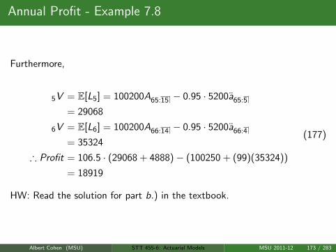
Annual Profit - Example 7.9
Define ASt as the share of the insurer’s assets attributable to each policyin force at time t. Consider now a policy identical to the policy studied inExample 7.4 amd suppose that this policy has now been in force for fiveyears. Suppose that over the past five years, the insurer’s experience inrespect of similar policies has realized annual interest on investments as(i1, i2, i3, i4, i5) = (0.048, 0.056, 0.052, 0.049, 0.047).
Albert Cohen (MSU) STT 455-6: Actuarial Models MSU 2011-12 174 / 283
Annual Profit - Example 7.9
Furthermore,
Expenses at the start of the year in which a policy was issued were15% of the premium
Expenses at the start of the year after the year in which a policy wasissued were 6% of the premium
The expense of paying a death claim was, on average, 120
The mortality rate q[50]+t ≈ 0.0015 for t ∈ 0, 1, 2, 3, 4
Calculate ASt using the convention that ASt does not include the premiumand related expense due at time t. (This of course means that AS0 = 0.)
Albert Cohen (MSU) STT 455-6: Actuarial Models MSU 2011-12 175 / 283
Annual Profit - Example 7.9
We calculate AS1 here and refer to Table 7.1 for the complete set ofcalculations
At time 0, insurer receives premiums minus expenses of0.85 · 11900N = 10115N.
At time 1, this accumulates to 10115N · (1 + i1) = 10601N.
A total of 0.0015N policy holders die in the first year and deathclaims are 0.0015N · (11900 + 120) = 18N.
Therefore, the value of the fund at the end of the first year is10601N − 18N = 10582N.
Albert Cohen (MSU) STT 455-6: Actuarial Models MSU 2011-12 176 / 283
Annual Profit - Example 7.9
It follows that
AS1 =Fund Value at time 1
Number of Policies in Force at time 1
=10582N
0.9985N= 10598
(178)
Now, read Section 7.4 on computing Valuation between premium dates.
Albert Cohen (MSU) STT 455-6: Actuarial Models MSU 2011-12 177 / 283
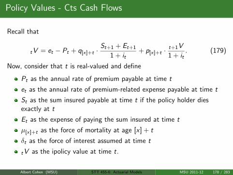
Policy Values - Cts Cash Flows
Recall that
tV = et − Pt + q[x]+t ·St+1 + Et+1
1 + it+ p[x]+t ·
t+1V
1 + it. (179)
Now, consider that t is real-valued and define
Pt as the annual rate of premium payable at time t
et as the annual rate of premium-related expense payable at time t
St as the sum insured payable at time t if the policy holder diesexactly at t
Et as the expense of paying the sum insured at time t
µ[x]+t as the force of mortality at age [x ] + t
δt as the force of interest assumed at time t
tV as the ipolicy value at time t.
Albert Cohen (MSU) STT 455-6: Actuarial Models MSU 2011-12 178 / 283

Policy Values - Cts Cash Flows
Now, as the force of interest varies, we have
v(t) = e−∫ t
0 δudu
v(t)
v(s)= e−
∫ ts δudu
(180)
and so
tV =
∫ ∞0
v(t + s)
v(t)·([St+s + Et+s ] · sp[x]+tµ[x]+t+s
)ds
−∫ ∞
0
v(t + s)
v(t)·([Pt+s − et+s ] · sp[x]+t
)ds
(181)
Q: What happens if there is a finite term to contract?
Albert Cohen (MSU) STT 455-6: Actuarial Models MSU 2011-12 179 / 283
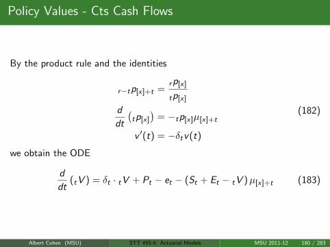
Policy Values - Cts Cash Flows
By the product rule and the identities
r−tp[x]+t =rp[x]
tp[x]
d
dt
(tp[x]
)= −tp[x]µ[x]+t
v ′(t) = −δtv(t)
(182)
we obtain the ODE
d
dt(tV ) = δt · tV + Pt − et − (St + Et − tV )µ[x]+t (183)
Albert Cohen (MSU) STT 455-6: Actuarial Models MSU 2011-12 180 / 283
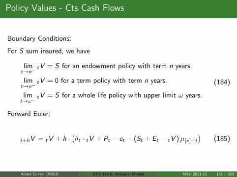
Policy Values - Cts Cash Flows
Boundary Conditions:
For S sum insured, we have
limt→n−
tV = S for an endowment policy with term n years.
limt→n−
tV = 0 for a term policy with term n years.
limt→ω−
tV = S for a whole life policy with upper limit ω years.
(184)
Forward Euler:
t+hV = tV + h ·(δt · tV + Pt − et − (St + Et − tV )µ[x]+t
)(185)
Albert Cohen (MSU) STT 455-6: Actuarial Models MSU 2011-12 181 / 283

Policy Values - Cts Cash Flows
As an example, consider the case where for S sum insured, we have
St+s = S
et+s = 0 = Et+s
δt = δ
µ[x]+t+s = λ
Pt+s = Pe−γ(t+s)
(186)
Then it follows that
tV =
∫ ∞0
Se−δs · λe−λsds −∫ ∞
0e−δs · Pe−γ(t+s)e−λsds
=Sλ
λ+ δ− Pe−γt
λ+ δ + γ
(187)
Albert Cohen (MSU) STT 455-6: Actuarial Models MSU 2011-12 182 / 283

Policy Alterations
In many cases, policyholders may wish to change the terms of theircontract if it is still in effect. For example:
They may wish to stop making premiums, or to change the terms oftheir benefit payout.
They may wish to cash out their position, or simply wish to shortenthe time remaining until payout.
One may argue that the insurer is under no obligation to make suchchanges if they are not written expressly into the initial contract. Forexample:
The policyholder (but not insurer) may know something about theirhealth status that would make it better for them to cash out now.
By having to liquidate assets that cover the policy, the insurer mayhave to take a loss to be able to settle the alteration, and this couldaffect other policyholders adversely.
Albert Cohen (MSU) STT 455-6: Actuarial Models MSU 2011-12 183 / 283
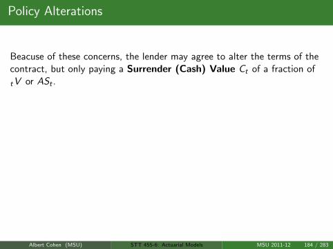
Policy Alterations
Beacuse of these concerns, the lender may agree to alter the terms of thecontract, but only paying a Surrender (Cash) Value Ct of a fraction of
tV or ASt .
Ct = E [PVt(future benefits + expenses, altered contract)]
− E [PVt(future premiums, altered contract)](188)
In allowing the policy to lapse, the policy holder is cashing out a policyand using the proceeds to enter into a new contract. If the period betweenlapsing and entering into a new contract is too short, then the insurer maysuffer from not earning enough income to cover the new business strain ofwriting the first contract. Hence, some countries including the US havenon-forfeiture laws that allow for zero cash values for early surrenders.
Albert Cohen (MSU) STT 455-6: Actuarial Models MSU 2011-12 184 / 283

Policy Alterations: Example 7.13
Consider the policy discussed in Examples 7.4 and 7.9. Given theexperience of the insurer detailed in Example 7.9, at the start of the 6th
year but before paying the premium due, the policyholder requests that thepolicy be altered in one of the following ways:
Albert Cohen (MSU) STT 455-6: Actuarial Models MSU 2011-12 185 / 283
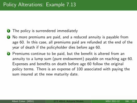
Policy Alterations: Example 7.13
1 The policy is surrendered immediately
2 No more premiums are paid, and a reduced annuity is payable fromage 60. In this case, all premiums paid are refunded at the end of theyear of death if the policyholder dies before age 60.
3 Premiums continue to be paid, but the benefit is altered from anannuity to a lump sum (pure endowment) payable on reaching age 60.Expenses and benefits on death before age 60 follow the originalpolicy terms. There is an expense of 100 associated with paying thesum insured at the new maturity date.
Albert Cohen (MSU) STT 455-6: Actuarial Models MSU 2011-12 186 / 283

Policy Alterations: Example 7.13
Calculate the surrender value, the reduced annuity, and sum insuredassuming the insurer uses
90% of the asset share less a charge of 200 or
95% of the policy value less a charge of 200
together with the assumptions in the policy value basis when calculatingrevised benefits and premimus. Use the associated values
5V = 65470
AS5 = 63509(189)
Albert Cohen (MSU) STT 455-6: Actuarial Models MSU 2011-12 187 / 283
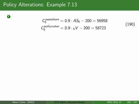
Policy Alterations: Example 7.13
1
C assetshare5 = 0.9 · AS5 − 200 = 56958
Cpolicyvalue5 = 0.9 · 5V − 200 = 58723
(190)
2
C5 = 5 · 11900A 155:5
+ 100A 155:5
+ (X + 25) · v 55p55 · a60
X assetshare = 4859
X policyvalue = 5012
(191)
3
C5 + 0.95 · 11900a55:5 = 11900(
(IA) 155:5
+ 5A 155:5
)+ 100A 1
55:5+ v 5
5p55 (S + 100)
Sassetshare = 138314
Spolicyvalue = 140594
(192)
Albert Cohen (MSU) STT 455-6: Actuarial Models MSU 2011-12 188 / 283
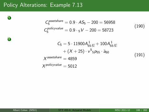
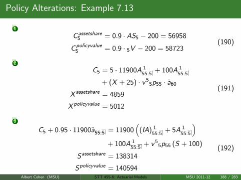
Related Project Topics
Over- or underestimated interest rates are only one risk factor foractuarial reserving. Another very real factor is known as longevityrisk, which is due to the possibility that a pensioner may live longerthan expected. Hedging against such a possibility is extremelyimportant, Please consult the paper by Tsai, Tzeng, and Wang onHedging Longevity Risk When Interest Rates Are Uncertain
Albert Cohen (MSU) STT 455-6: Actuarial Models MSU 2011-12 189 / 283

Related Project Topics
For those of you interested in more sophisitcated, cutting edge codingmethods for reserving, code.google.com has a site dedicated toChainLadder (google code name chainladder) that contains an Rpackage providing methods which are typically used in insuranceclaims reserving. Links to slides explaining the method are also on thesite
An Introduction to R: Examples for Actuaries by Nigel de Silva is avery nice primer on using R.
Albert Cohen (MSU) STT 455-6: Actuarial Models MSU 2011-12 190 / 283

Homework Questions
HW: 7.1, 7.2, 7.4, 7.5, 7.8, 7.12, 7.14, 7.15
Albert Cohen (MSU) STT 455-6: Actuarial Models MSU 2011-12 191 / 283
Two State Model: Alive or Dead
Recall that for the survival time Tx of an individual (x), we have
Sx(t) = 1− Fx(t) = 1− P[Tx ≤ t] (193)
We now extend the model to include multiple states, but first we definethe random variable Y (t) ∈ 0, 1 as the state of the individual (x). If (x)is alive at time x + t, then Y (t) = 0. Otherwise, Y (t) = 1.Hence, we can define
Tx = max t | Y (t) = 0 (194)
and the model flow 0→ 1.
Albert Cohen (MSU) STT 455-6: Actuarial Models MSU 2011-12 192 / 283
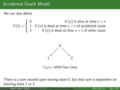
Accidental Death Model
We can also define
Y (t) =
0 if (x) is alive at time x + t1 if (x) is dead at time x + t of accidental cause2 if (x) is dead at time x + t of other cause
0
>>>>>>>>
1 2
Figure: ADM Flow Chart
There is a sum insured upon leaving state 0, but that sum is dependent onentering state 1 or 2.
Albert Cohen (MSU) STT 455-6: Actuarial Models MSU 2011-12 193 / 283
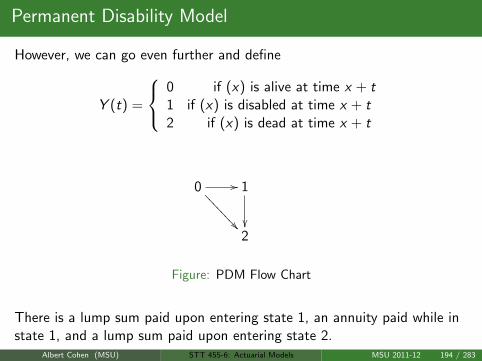
Permanent Disability Model
However, we can go even further and define
Y (t) =
0 if (x) is alive at time x + t1 if (x) is disabled at time x + t2 if (x) is dead at time x + t
0 //
>>>>>>>> 1
2
Figure: PDM Flow Chart
There is a lump sum paid upon entering state 1, an annuity paid while instate 1, and a lump sum paid upon entering state 2.
Albert Cohen (MSU) STT 455-6: Actuarial Models MSU 2011-12 194 / 283
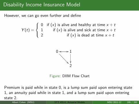
Disability Income Insurance Model
However, we can go even further and define
Y (t) =
0 if (x) is alive and healthy at time x + t1 if (x) is alive and sick at time x + t2 if (x) is dead at time x + t
0 //
>>>>>>>> 1oo
2
Figure: DIIM Flow Chart
Premium is paid while in state 0, is a lump sum paid upon entering state1, an annuity paid while in state 1, and a lump sum paid upon enteringstate 2.
Albert Cohen (MSU) STT 455-6: Actuarial Models MSU 2011-12 195 / 283

Joint Life - Last Survivor
Define
Joint Life Annuity - annuity that pays until the first death among agroup of lives
Last Survivor Annuity - annuity that pays until the last deathamong a group of lives
A common feature is payment rate decreases upon each death
Reversionary Annuity - life annuity that starts payment upon deathof a specified life, as long as another member of group is alive
Joint Life Insurance - life annuity that starts payment upon firstdeath of a member of group
Usually, group consists of two members, a husband and a wife
Albert Cohen (MSU) STT 455-6: Actuarial Models MSU 2011-12 196 / 283

Joint Model
For example, consider a policy issued to a group (H,W ) of age x , y).Then,
Y (t) =
0 if H is alive at x + t and W is alive at y + t1 if H is alive at x + t and W is dead at y + t2 if H is dead at x + t and W is alive at y + t3 if H is dead at x + t and W is dead at y + t
0 //
1
2 // 3
Figure: Joint Model Flow Chart
Albert Cohen (MSU) STT 455-6: Actuarial Models MSU 2011-12 197 / 283
Notation
Assuming that the group (which can consist of 1,2, or more individuals)can be found in an of the the n + 1 states 0, 1, 2, ..., n − 1, n, we definethe event
Y (t) = i (195)
to mean the group is in state i at time t.
It follows that Y (t)t≥0 is a discrete valued stochastic process.
Albert Cohen (MSU) STT 455-6: Actuarial Models MSU 2011-12 198 / 283
Assumptions
We make the following assumptions and definitions about transitionsbetween states and their associated probabilities:
P[Y (x + t) = j | Y (x) = i ] := tpijx (Markovity)
P[Y (x + s) = i for all s ∈ [0, t] | Y (x) = i ] := tpiix
limh→0
P[2 or more transitions in interval of length h]
h= 0
limh→0+
hpijx
h:= µijx
d
dt
(tp
ijx
)exists for all t ≥ 0
(196)
Albert Cohen (MSU) STT 455-6: Actuarial Models MSU 2011-12 199 / 283
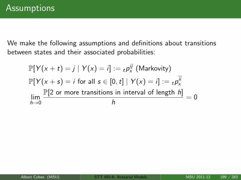
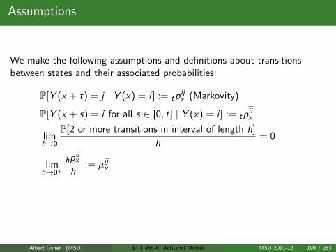
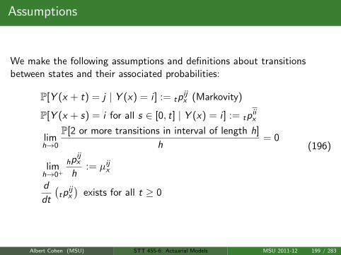

Note:
Note that
tp00x = tpx
tp01x = tqx
tp10x = 0
0pijx = 1i=j
µ01x = µx
hpijx = h · µijx + o(h)
tpiix ≤ tp
iix
(197)
Albert Cohen (MSU) STT 455-6: Actuarial Models MSU 2011-12 200 / 283

Note:
Note that
tp00x = tpx
tp01x = tqx
tp10x = 0
0pijx = 1i=j
µ01x = µx
hpijx = h · µijx + o(h)
tpiix ≤ tp
iix
(197)
Albert Cohen (MSU) STT 455-6: Actuarial Models MSU 2011-12 200 / 283

Example 8.2− 3
We can in fact show that
hpiix = 1− h ·
n∑j=0,j 6=i
µijx + o(h)
tpiix = exp
−∫ t
0
n∑j=0,j 6=i
µijx+sds
(198)
See proof in book.
As an example, we can show that for the permanent disability model, wehave
up01x =
∫ u
0tp
00x · µ01
x+t · u−tp11x+tdt (199)
Albert Cohen (MSU) STT 455-6: Actuarial Models MSU 2011-12 201 / 283

Example 8.2− 3
We can in fact show that
hpiix = 1− h ·
n∑j=0,j 6=i
µijx + o(h)
tpiix = exp
−∫ t
0
n∑j=0,j 6=i
µijx+sds
(198)
See proof in book.As an example, we can show that for the permanent disability model, wehave
up01x =
∫ u
0tp
00x · µ01
x+t · u−tp11x+tdt (199)
Albert Cohen (MSU) STT 455-6: Actuarial Models MSU 2011-12 201 / 283
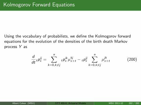
Kolmogorov Forward Equations
Using the vocabulary of probabilists, we define the Kolmogorov forwardequations for the evolution of the densities of the birth death Markovprocess Y as
d
dttp
ijx =
n∑k=0,k 6=j
tpikx µ
kjx+t − tp
ijx
n∑k=0,k 6=j
µjkx+t (200)
Albert Cohen (MSU) STT 455-6: Actuarial Models MSU 2011-12 202 / 283

Kolmogorov Forward Equations
In matrix notation, for a fixed x , define the matrices P(t),Q(t) such that
[P(t)]i ,j = tpijx
Q(t) =
−∑n
k=1 µ0kx+t µ01
x+t · · · µ0nx+t
µ10x+t −
∑nk=0,k 6=1 µ
1kx+t · · · µ1n
x+t...
.... . .
...
µn0x+t µn1
x+t · · · −∑n−1
k=0 µnkx+t
(201)
and the corresponding ODE system is
P ′(t) = P(t)Q(t)
P(0) = I = Identity Matrix.(202)
Albert Cohen (MSU) STT 455-6: Actuarial Models MSU 2011-12 203 / 283
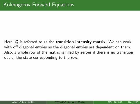
Kolmogorov Forward Equations
Here, Q is referred to as the transition intensity matrix. We can workwith off diagonal entries as the diagonal entries are dependent on them.Also, a whole row of the matrix is filled by zeroes if there is no transitionout of the state corresponding to the row.
Albert Cohen (MSU) STT 455-6: Actuarial Models MSU 2011-12 204 / 283
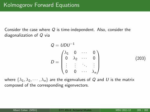
Kolmogorov Forward Equations
Consider the case where Q is time-independent. Also, consider thediagonalization of Q via
Q = UDU−1
D =
λ1 0 · · · 00 λ2 · · · 0...
.... . .
...0 0 · · · λn
(203)
where λ1, λ2, · · · , λn are the eigenvalues of Q and U is the matrixcomposed of the corresponding eigenvectors.
Albert Cohen (MSU) STT 455-6: Actuarial Models MSU 2011-12 205 / 283
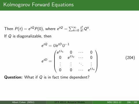
Kolmogorov Forward Equations
Then P(t) = etQP(0), where etQ =∑∞
k=0tk
k! Qk .
If Q is diagonalizable, then
etQ = UetDU−1
etD =
etλ1 0 · · · 0
0 etλ2 · · · 0...
.... . .
...0 0 · · · etλn
(204)
Question: What if Q is in fact time dependent?
Albert Cohen (MSU) STT 455-6: Actuarial Models MSU 2011-12 206 / 283
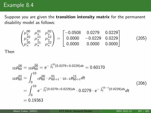
Example 8.4
Suppose you are given the transition intensity matrix for the permanentdisability model as follows:µ00
x µ01x µ02
x
µ10x µ11
x µ12x
µ20x µ21
x µ22x
=
−0.0508 0.0279 0.02290.0000 −0.0229 0.02290.0000 0.0000 0.0000
(205)
Then
10p0060 = 10p00
60 = e−∫ 10
0 (0.0279+0.0229)ds = 0.60170
10p0160 =
∫ 10
0tp
0060 · µ01
60+t · 10−tp1160+tdt
=
∫ 10
0e−
∫ t0 (0.0279+0.0229)ds · 0.0279 · e−
∫ 10−t0 (0.0229)dsdt
= 0.19363
(206)
Albert Cohen (MSU) STT 455-6: Actuarial Models MSU 2011-12 207 / 283
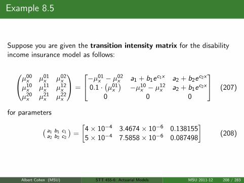
Example 8.5
Suppose you are given the transition intensity matrix for the disabilityincome insurance model as follows:
µ00x µ01
x µ02x
µ10x µ11
x µ12x
µ20x µ21
x µ22x
=
−µ01x − µ02
x a1 + b1ec1x a2 + b2ec2x
0.1 ·(µ01x
)−µ10
x − µ12x a2 + b1ec2x
0 0 0
(207)
for parameters
(a1 b1 c1a2 b2 c2
)=
[4× 10⁻⁴ 3.4674× 10⁻⁶ 0.1381555× 10⁻⁴ 7.5858× 10⁻⁶ 0.087498
](208)
Albert Cohen (MSU) STT 455-6: Actuarial Models MSU 2011-12 208 / 283
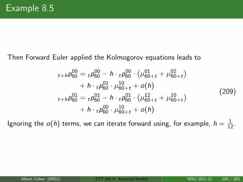
Example 8.5
Then Forward Euler applied the Kolmogorov equations leads to
t+hp0060 = tp
0060 − h · tp00
60 ·(µ01
60+t + µ0260+t
)+ h · tp01
60 · µ1060+t + o(h)
t+hp0160 = tp
0160 − h · tp01
60 ·(µ12
60+t + µ1060+t
)+ h · tp00
60 · µ1060+t + o(h)
(209)
Ignoring the o(h) terms, we can iterate forward using, for example, h = 112 .
Albert Cohen (MSU) STT 455-6: Actuarial Models MSU 2011-12 209 / 283

Example 8.5
In matrix-vector notation, we have(t+hp00
60
t+hp0160
)= [I− hA(t)]
(tp
0060
tp0160
)
I =
(1 00 1
)A(t) =
(µ01
60+t + µ0260+t −µ10
60+t
−µ1060+t µ12
60+t + µ1060+t
) (210)
Keep in mind that A is determined by the given transition intensity matrix.
HW Compute this vector over the interval t ∈ [0, 10] using a time step ofh = 1
12 . Use any numerical solver you like, but please have the valuescomputed into a pair of columns.
Albert Cohen (MSU) STT 455-6: Actuarial Models MSU 2011-12 210 / 283

Example 8.5
In matrix-vector notation, we have(t+hp00
60
t+hp0160
)= [I− hA(t)]
(tp
0060
tp0160
)I =
(1 00 1
)A(t) =
(µ01
60+t + µ0260+t −µ10
60+t
−µ1060+t µ12
60+t + µ1060+t
) (210)
Keep in mind that A is determined by the given transition intensity matrix.
HW Compute this vector over the interval t ∈ [0, 10] using a time step ofh = 1
12 . Use any numerical solver you like, but please have the valuescomputed into a pair of columns.
Albert Cohen (MSU) STT 455-6: Actuarial Models MSU 2011-12 210 / 283
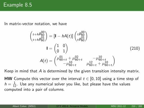
Example 8.5
In matrix-vector notation, we have(t+hp00
60
t+hp0160
)= [I− hA(t)]
(tp
0060
tp0160
)I =
(1 00 1
)A(t) =
(µ01
60+t + µ0260+t −µ10
60+t
−µ1060+t µ12
60+t + µ1060+t
) (210)
Keep in mind that A is determined by the given transition intensity matrix.
HW Compute this vector over the interval t ∈ [0, 10] using a time step ofh = 1
12 . Use any numerical solver you like, but please have the valuescomputed into a pair of columns.
Albert Cohen (MSU) STT 455-6: Actuarial Models MSU 2011-12 210 / 283
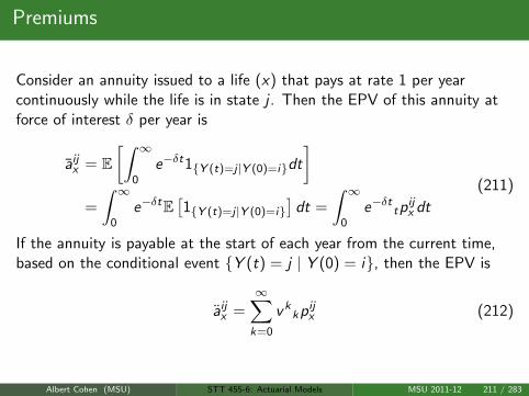
Premiums
Consider an annuity issued to a life (x) that pays at rate 1 per yearcontinuously while the life is in state j . Then the EPV of this annuity atforce of interest δ per year is
aijx = E[∫ ∞
0e−δt1Y (t)=j |Y (0)=idt
]=
∫ ∞0
e−δtE[1Y (t)=j |Y (0)=i
]dt =
∫ ∞0
e−δt tpijx dt
(211)
If the annuity is payable at the start of each year from the current time,based on the conditional event Y (t) = j | Y (0) = i, then the EPV is
aijx =∞∑k=0
vkkpij
x (212)
Albert Cohen (MSU) STT 455-6: Actuarial Models MSU 2011-12 211 / 283

Premiums
If a unit benefit is payable to a life (x) on transition to state k , given thatit is currently in state i , then the EPV of this benefit is
Aikx =
∫ ∞0
∑j 6=k
e−δt tpijx µ
jkx+tdt (213)
Albert Cohen (MSU) STT 455-6: Actuarial Models MSU 2011-12 212 / 283

Example 8.6
An insurer issues a 10−year disability income insurance policy to a healthylife aged 60. Use the model and parameters from Example 8.5. Assume aneffective rate of 5% per year and no expenses. Calculate the premiums forthe following designs
(a) Premiums are payable continuously while in the healthy state. Abenefit of 20000 per year is payable continuously while in the disabledstate. A death benefit of 50000 is payable immediately upon death.
(b) Premiums are payable monthly in advance conditional on the lifebeing in the healthy state at the premium date. The sickness benefitof 20000 per year is payable monthly in arrear, if the life is in the sickstate at the payment date. A death benefit of 50000 is payableimmediatlely upon death.
Albert Cohen (MSU) STT 455-6: Actuarial Models MSU 2011-12 213 / 283
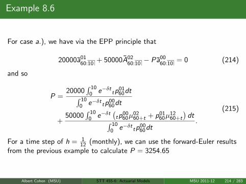
Example 8.6
For case a.), we have via the EPP principle that
20000a0160:10
+ 50000A0260:10
− Pa0060:10
= 0 (214)
and so
P =20000
∫ 100 e−δt tp
0160dt∫ 10
0 e−δt tp0060dt
+50000
∫ 100 e−δt
(tp
0060µ
0260+t + p01
60µ1260+t
)dt∫ 10
0 e−δt tp0060dt
.
(215)
For a time step of h = 112 (monthly), we can use the forward-Euler results
from the previous example to calculate P = 3254.65
Albert Cohen (MSU) STT 455-6: Actuarial Models MSU 2011-12 214 / 283
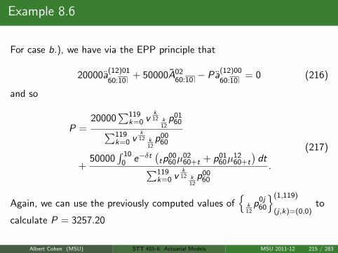
Example 8.6
For case b.), we have via the EPP principle that
20000a(12)01
60:10+ 50000A02
60:10− Pa
(12)00
60:10= 0 (216)
and so
P =20000
∑119k=0 v
k12 k
12p01
60∑119k=0 v
k12 k
12p00
60
+50000
∫ 100 e−δt
(tp
0060µ
0260+t + p01
60µ1260+t
)dt∑119
k=0 vk12 k
12p00
60
.
(217)
Again, we can use the previously computed values of
k12
p0j60
(1,119)
(j ,k)=(0,0)to
calculate P = 3257.20
Albert Cohen (MSU) STT 455-6: Actuarial Models MSU 2011-12 215 / 283
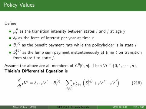
Policy Values
Define
µijy as the transition intensity between states i and j at age y
δt as the force of interest per year at time t
B(i)t as the benefit payment rate while the policyholder is in state i
S(ij)t as the lump sum payment instantaneously at time t on transition
from state i to state j .
Assume the above are all members of C 0[0, n]. Then ∀i ∈ 0, 1, · · · , n,Thiele’s Differential Equation is
d
dttV
i = δt · tV i − B(i)t −
∑j 6=i
µijx+t
(S
(ij)t + tV
j − tVi)
(218)
Albert Cohen (MSU) STT 455-6: Actuarial Models MSU 2011-12 216 / 283
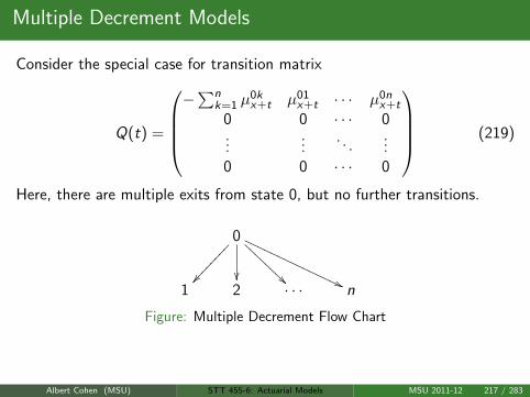
Multiple Decrement Models
Consider the special case for transition matrix
Q(t) =
−∑n
k=1 µ0kx+t µ01
x+t · · · µ0nx+t
0 0 · · · 0...
.... . .
...0 0 · · · 0
(219)
Here, there are multiple exits from state 0, but no further transitions.
0
AAAAAAAA
''PPPPPPPPPPPPPPP
1 2 · · · n
Figure: Multiple Decrement Flow Chart
Albert Cohen (MSU) STT 455-6: Actuarial Models MSU 2011-12 217 / 283
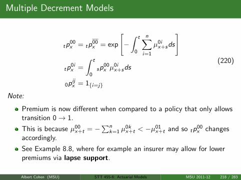
Multiple Decrement Models
tp00x = tp
00x = exp
[−∫ t
0
n∑i=1
µ0ix+sds
]
tp0ix =
∫ t
0sp00
x µ0ix+sds
0pijx = 1i=j
(220)
Note:
Premium is now different when compared to a policy that only allowstransition 0→ 1.
This is because µ00x+t = −
∑nk=1 µ
0kx+t < −µ01
x+t and so tp00x changes
accordingly.
See Example 8.8, where for example an insurer may allow for lowerpremiums via lapse support.
Albert Cohen (MSU) STT 455-6: Actuarial Models MSU 2011-12 218 / 283

Joint Life - Last Survivor Benefits
0µ01x+t:y+t//
µ02x+t:y+t
1
µ13x+t
2µ23y+t
// 3
Figure: Joint Model Transition Rates
Define the joint transition matrix via the flow chart above.
Albert Cohen (MSU) STT 455-6: Actuarial Models MSU 2011-12 219 / 283

Joint Life - Last Survivor Benefits
Define
tpxy = tp00xy = P[(x) and (y) are both alive in t years]
tqxy = tp01xy + tp
02xy + tp
03xy
= P[(x) and (y) are not both alive in t years]
tpxy = tp00xy + tp
01xy + tp
02xy
= P[ at least one of (x) and (y) is alive in t years]
tqxy = 1− tpxy
µx+t:y+t = µ01x+t:y+t + µ02
x+t:y+t
(221)
Albert Cohen (MSU) STT 455-6: Actuarial Models MSU 2011-12 220 / 283
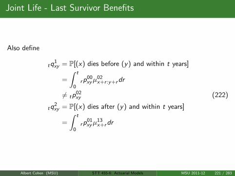
Joint Life - Last Survivor Benefits
Also define
tq1xy = P[(x) dies before (y) and within t years]
=
∫ t
0rp00
xyµ02x+r :y+rdr
6= tp02xy
tq2xy = P[(x) dies after (y) and within t years]
=
∫ t
0rp01
xyµ13x+rdr
(222)
Albert Cohen (MSU) STT 455-6: Actuarial Models MSU 2011-12 221 / 283

Joint Life - Last Survivor Benefits
Insurance Notation
axy = a00xy , the Joint Life Annuity with continuous payment of 1 per
year while both husband and wife are alive.
Axy the Joint Life Insurance with a unit payment immediately uponfirst death.
A1xy , the Contingent Insurance, a unit payment immediately upon
death of the husband given that he dies before his wife.
Albert Cohen (MSU) STT 455-6: Actuarial Models MSU 2011-12 222 / 283

Joint Life - Last Survivor Benefits
Insurance Notation
Axy = A03xy , the Last Survivor Insurance with unit payment
immediately upon second death.
ax |y = a02xy the Reversionary Annuity with a continuous payment at
unit rate per year while wife is alive given that husband has died..
axy = a00xy + a01
xy + a02xy , the Last Survivor Annuity, a continuous
payment at rate 1 per year while at least one person is alive.
Albert Cohen (MSU) STT 455-6: Actuarial Models MSU 2011-12 223 / 283

Joint Life - Last Survivor Benefits
It can be shown that
axy = ax + ay − axy
ax |y = ay − axy
Axy = Ax + Ay − Axy
axy =1− Axy
δ
(223)
HW
Prove this using explicit integral formulations.
Read over Examples 8.10 and 8.11.
Albert Cohen (MSU) STT 455-6: Actuarial Models MSU 2011-12 224 / 283
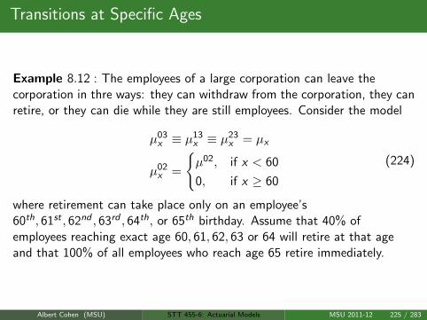
Transitions at Specific Ages
Example 8.12 : The employees of a large corporation can leave thecorporation in thre ways: they can withdraw from the corporation, they canretire, or they can die while they are still employees. Consider the model
µ03x ≡ µ13
x ≡ µ23x = µx
µ02x =
µ02, if x < 60
0, if x ≥ 60
(224)
where retirement can take place only on an employee’s60th, 61st , 62nd , 63rd , 64th, or 65th birthday. Assume that 40% ofemployees reaching exact age 60, 61, 62, 63 or 64 will retire at that ageand that 100% of all employees who reach age 65 retire immediately.
Albert Cohen (MSU) STT 455-6: Actuarial Models MSU 2011-12 225 / 283
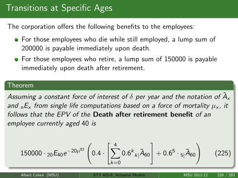
Transitions at Specific Ages
The corporation offers the following benefits to the employees:
For those employees who die while still employed, a lump sum of200000 is payable immediately upon death.
For those employees who retire, a lump sum of 150000 is payableimmediately upon death after retirement.
Theorem
Assuming a constant force of interest of δ per year and the notation of Ax
and nEx from single life computations based on a force of mortality µx , itfollows that the EPV of the Death after retirement benefit of anemployee currently aged 40 is
150000 · 20E40e−20µ02
(0.4 ·
[4∑
k=0
0.6kk|A60
]+ 0.65 · 5|A60
)(225)
Albert Cohen (MSU) STT 455-6: Actuarial Models MSU 2011-12 226 / 283
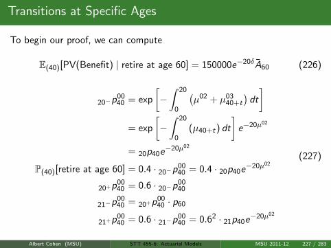
Transitions at Specific Ages
To begin our proof, we can compute
E(40)[PV(Benefit) | retire at age 60] = 150000e−20δA60 (226)
20−p0040 = exp
[−∫ 20
0
(µ02 + µ03
40+t
)dt
]= exp
[−∫ 20
0(µ40+t) dt
]e−20µ02
= 20p40e−20µ02
P(40)[retire at age 60] = 0.4 · 20−p0040 = 0.4 · 20p40e−20µ02
20+p0040 = 0.6 · 20−p00
40
21−p0040 = 20+p00
40 · p60
21+p0040 = 0.6 · 21−p00
40 = 0.62 · 21p40e−20µ02
(227)
Albert Cohen (MSU) STT 455-6: Actuarial Models MSU 2011-12 227 / 283
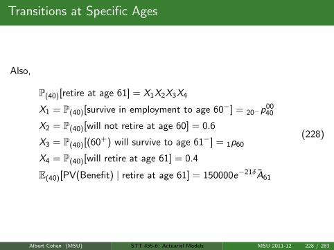
Transitions at Specific Ages
Also,
P(40)[retire at age 61] = X1X2X3X4
X1 = P(40)[survive in employment to age 60−] = 20−p0040
X2 = P(40)[will not retire at age 60] = 0.6
X3 = P(40)[(60+) will survive to age 61−] = 1p60
X4 = P(40)[will retire at age 61] = 0.4
E(40)[PV(Benefit) | retire at age 61] = 150000e−21δA61
(228)
Albert Cohen (MSU) STT 455-6: Actuarial Models MSU 2011-12 228 / 283
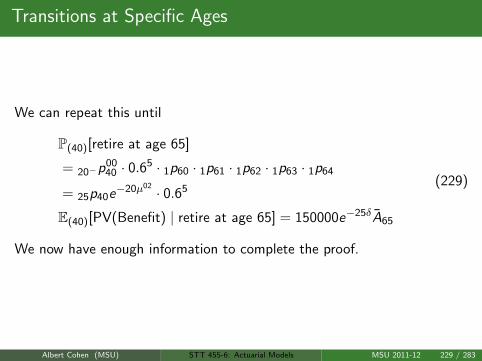
Transitions at Specific Ages
We can repeat this until
P(40)[retire at age 65]
= 20−p0040 · 0.65 · 1p60 · 1p61 · 1p62 · 1p63 · 1p64
= 25p40e−20µ02 · 0.65
E(40)[PV(Benefit) | retire at age 65] = 150000e−25δA65
(229)
We now have enough information to complete the proof.
Albert Cohen (MSU) STT 455-6: Actuarial Models MSU 2011-12 229 / 283

Transitions at Specific Ages
Proof.
For benefit after retirement, we have
E(40)[PV(Benefit)] =5∑
k=0
Bk(40)P
k(40)
Bk(40) = E(40)[PV(Benefit) | retire at age 60 + k]
= 150000e−(20+k)δA60+k for k ∈ 0, · · · , 5Pk
(40) := P(40)[retire at age 60 + k]
= 20+kp40e−20µ02 · 0.6k · 0.4 for k ∈ 0, · · · , 4
P5(40) = 25p40e−20µ02 · 0.65
(230)
Substitution and arithmetic lead to the form in the theorem statement.
Albert Cohen (MSU) STT 455-6: Actuarial Models MSU 2011-12 230 / 283
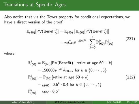
Transitions at Specific Ages
Also notice that via the Tower property for conditional expectations, wehave a direct version of the proof:
E(40)[PV(Benefit)] = E(40)
[E(60)[PV(Benefit)]
]= 20E40e−20µ02 ·
5∑k=0
Bk(60)P
k(60)
(231)
where
Bk(60) = E(60)[PV(Benefit) | retire at age 60 + k]
= 150000e−kδA60+k for k ∈ 0, · · · , 5Pk
(60) := P(60)[retire at age 60 + k]
= kp60 · 0.6k · 0.4 for k ∈ 0, · · · , 4P5
(60) = 5p60 · 0.65
(232)
Albert Cohen (MSU) STT 455-6: Actuarial Models MSU 2011-12 231 / 283

Homework Questions
HW: 8.1, 8.2, 8.4, 8.5, 8.8, 8.10, 8.11, 8.15, 8.16, 8.21, 8.22
Albert Cohen (MSU) STT 455-6: Actuarial Models MSU 2011-12 232 / 283

Plan Type
We consider two types of retirement plans.
A Defined Contribution plan specifies how much an employer willcontribute, as a percentage of salary, into a plan.
A Defined Benefit plan specifies a level of benefit, most likelyrelated to the employee’s salary near retirement. Here, contributionsmay need to be updated based on the investment returns to ensurethat the benefit is met.
Albert Cohen (MSU) STT 455-6: Actuarial Models MSU 2011-12 233 / 283
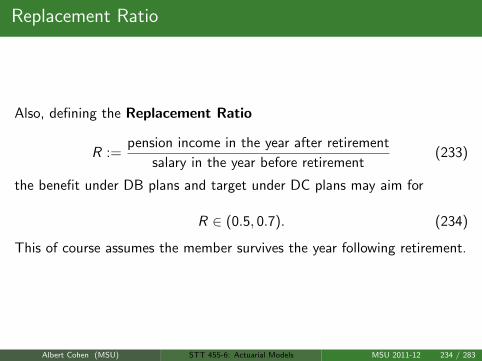
Replacement Ratio
Also, defining the Replacement Ratio
R :=pension income in the year after retirement
salary in the year before retirement(233)
the benefit under DB plans and target under DC plans may aim for
R ∈ (0.5, 0.7). (234)
This of course assumes the member survives the year following retirement.
Albert Cohen (MSU) STT 455-6: Actuarial Models MSU 2011-12 234 / 283
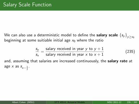
Salary Scale Function
We can also use a deterministic model to define the salary scale syy≥x0
beginning at some suitiable initial age x0 where the ratio
sysx
=salary received in year y to y + 1
salary received in year x to x + 1(235)
and, assuming that salaries are increased continuously, the salary rate atage x as sx− 1
2.
Albert Cohen (MSU) STT 455-6: Actuarial Models MSU 2011-12 235 / 283
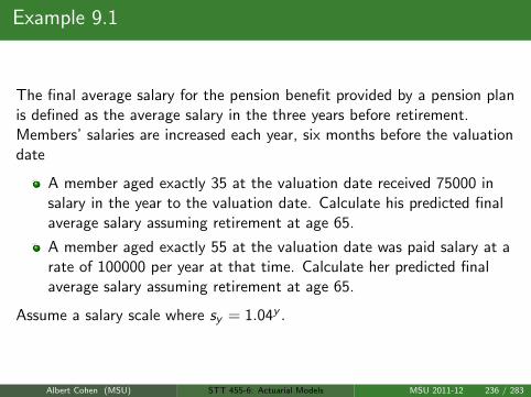
Example 9.1
The final average salary for the pension benefit provided by a pension planis defined as the average salary in the three years before retirement.Members’ salaries are increased each year, six months before the valuationdate
A member aged exactly 35 at the valuation date received 75000 insalary in the year to the valuation date. Calculate his predicted finalaverage salary assuming retirement at age 65.
A member aged exactly 55 at the valuation date was paid salary at arate of 100000 per year at that time. Calculate her predicted finalaverage salary assuming retirement at age 65.
Assume a salary scale where sy = 1.04y .
Albert Cohen (MSU) STT 455-6: Actuarial Models MSU 2011-12 236 / 283

Example 9.1
For first case
savg = 75000 · 1
3
s62 + s63 + s64
s34
=75000
3·(1.0428 + 1.0429 + 1.0430
)= 234019
(236)
For second case
savg = 100000 · 1
3
s62 + s63 + s64
s54.5
=100000
3·(1.047.5 + 1.048.5 + 1.049.5
)= 139639
(237)
Now read Example 9.2 for more practice and Example 9.3 for setting theDC contribution.
Albert Cohen (MSU) STT 455-6: Actuarial Models MSU 2011-12 237 / 283
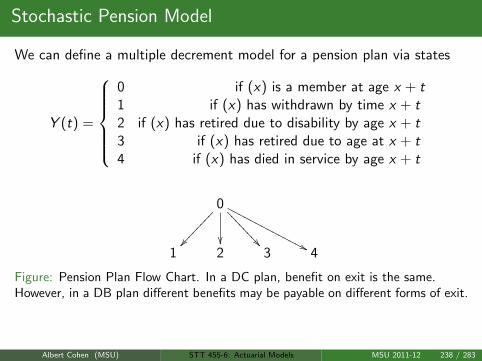
Stochastic Pension Model
We can define a multiple decrement model for a pension plan via states
Y (t) =
0 if (x) is a member at age x + t1 if (x) has withdrawn by time x + t2 if (x) has retired due to disability by age x + t3 if (x) has retired due to age at x + t4 if (x) has died in service by age x + t
0
>>>>>>>>
''NNNNNNNNNNNNNN
1 2 3 4
Figure: Pension Plan Flow Chart. In a DC plan, benefit on exit is the same.However, in a DB plan different benefits may be payable on different forms of exit.
Albert Cohen (MSU) STT 455-6: Actuarial Models MSU 2011-12 238 / 283
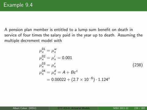
Example 9.4
A pension plan member is entitled to a lump sum benefit on death inservice of four times the salary paid in the year up to death. Assuming themultiple decrement model with
µ01x = µwx
µ02x = µix = 0.001
µ03x = µrx
µ04x = µdx = A + Bcx
= 0.00022 + (2.7× 10−6) · 1.124x
(238)
Albert Cohen (MSU) STT 455-6: Actuarial Models MSU 2011-12 239 / 283
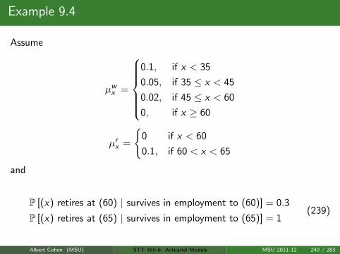
Example 9.4
Assume
µwx =
0.1, if x < 35
0.05, if 35 ≤ x < 45
0.02, if 45 ≤ x < 60
0, if x ≥ 60
µrx =
0 if x < 60
0.1, if 60 < x < 65
and
P [(x) retires at (60) | survives in employment to (60)] = 0.3
P [(x) retires at (65) | survives in employment to (65)] = 1(239)
Albert Cohen (MSU) STT 455-6: Actuarial Models MSU 2011-12 240 / 283
Example 9.4
Calculate, for a member aged 35, the probability of retiring at age 65.Notice the similarities to Example 8.12.
For t ∈ (0, 10), we have
tp0035 = exp
[−∫ t
0
(µw35+s + µi35+s + µr35+s + µd35+s
)ds
]= exp
[−∫ t
0
(0.05 + 0.001 + 0 + A + Bc35+s
)ds
]= exp
[−0.05122t +
2.7× 10⁻⁶
ln (1.124)1.12435
(1.124t − 1
)](240)
It follows that 10p0035 = 0.597342
Albert Cohen (MSU) STT 455-6: Actuarial Models MSU 2011-12 241 / 283
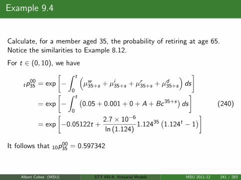
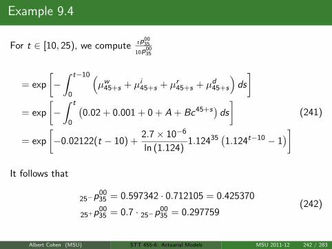
Example 9.4
For t ∈ [10, 25), we compute tp0035
10p0035
= exp
[−∫ t−10
0
(µw45+s + µi45+s + µr45+s + µd45+s
)ds
]= exp
[−∫ t
0
(0.02 + 0.001 + 0 + A + Bc45+s
)ds
]= exp
[−0.02122(t − 10) +
2.7× 10⁻⁶
ln (1.124)1.12435
(1.124t−10 − 1
)](241)
It follows that
25−p0035 = 0.597342 · 0.712105 = 0.425370
25+p0035 = 0.7 · 25−p00
35 = 0.297759(242)
Albert Cohen (MSU) STT 455-6: Actuarial Models MSU 2011-12 242 / 283
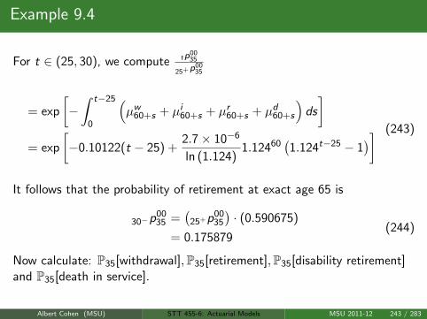
Example 9.4
For t ∈ (25, 30), we compute tp0035
25+p0035
= exp
[−∫ t−25
0
(µw60+s + µi60+s + µr60+s + µd60+s
)ds
]= exp
[−0.10122(t − 25) +
2.7× 10⁻⁶
ln (1.124)1.12460
(1.124t−25 − 1
)] (243)
It follows that the probability of retirement at exact age 65 is
30−p0035 =
(25+p00
35
)· (0.590675)
= 0.175879(244)
Now calculate: P35[withdrawal],P35[retirement],P35[disability retirement]and P35[death in service].
Albert Cohen (MSU) STT 455-6: Actuarial Models MSU 2011-12 243 / 283
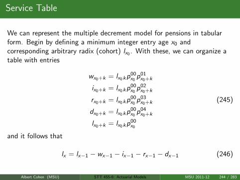
Service Table
We can represent the multiple decrement model for pensions in tabularform. Begin by defining a minimum integer entry age x0 andcorresponding arbitrary radix (cohort) lx0 . With these, we can organize atable with entries
wx0+k = lx0kp00x0
p01x0+k
ix0+k = lx0kp00x0
p02x0+k
rx0+k = lx0kp00x0
p03x0+k
dx0+k = lx0kp00x0
p04x0+k
lx0+k = lx0kp00x0
(245)
and it follows that
lx = lx−1 − wx−1 − ix−1 − rx−1 − dx−1 (246)
Albert Cohen (MSU) STT 455-6: Actuarial Models MSU 2011-12 244 / 283
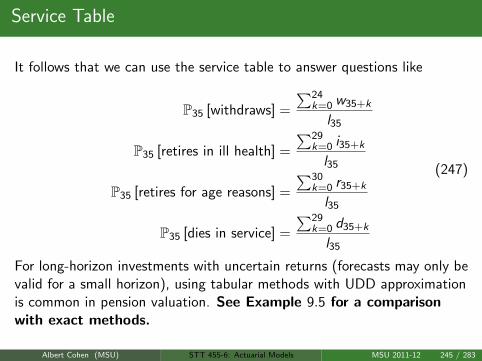
Service Table
It follows that we can use the service table to answer questions like
P35 [withdraws] =
∑24k=0 w35+k
l35
P35 [retires in ill health] =
∑29k=0 i35+k
l35
P35 [retires for age reasons] =
∑30k=0 r35+k
l35
P35 [dies in service] =
∑29k=0 d35+k
l35
(247)
For long-horizon investments with uncertain returns (forecasts may only bevalid for a small horizon), using tabular methods with UDD approximationis common in pension valuation. See Example 9.5 for a comparisonwith exact methods.
Albert Cohen (MSU) STT 455-6: Actuarial Models MSU 2011-12 245 / 283
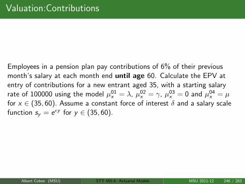
Valuation:Contributions
Employees in a pension plan pay contributions of 6% of their previousmonth’s salary at each month end until age 60. Calculate the EPV atentry of contributions for a new entrant aged 35, with a starting salaryrate of 100000 using the model µ01
x = λ, µ02x = γ, µ03
x = 0 and µ04x = µ
for x ∈ (35, 60). Assume a constant force of interest δ and a salary scalefunction sy = eεy for y ∈ (35, 60).
Albert Cohen (MSU) STT 455-6: Actuarial Models MSU 2011-12 246 / 283
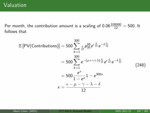
Valuation
Per month, the contribution amount is a scaling of 0.06 10000012 = 500. It
follows that
E [PV(Contributions)] = 500300∑k=1
k12
p0035eε
k12 e−δ
k12
= 500300∑k=1
e−(µ+γ+λ) k12 eε
k12 e−δ
k12
= 500ex
1− ex1− e300x
x =ε− µ− γ − λ− δ
12
(248)
Albert Cohen (MSU) STT 455-6: Actuarial Models MSU 2011-12 247 / 283
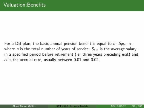
Valuation:Benefits
For a DB plan, the basic annual pension benefit is equal to n · SFin · α,where n is the total number of years of service, SFin is the average salaryin a specified period before retirement (ie. three years preceding exit) andα is the accrual rate, usually between 0.01 and 0.02.
Albert Cohen (MSU) STT 455-6: Actuarial Models MSU 2011-12 248 / 283

Valuation:Benefits; Example 9.6
Estimate the EPV of the accrued age retirement pension benefit for amember aged 55 with 20 years of service, whose salary in the year prior tothe valuation date was 50000. Assume that mid-year age retirementshappen at exactly halfway into the year. Assume the final average salary isdefined as the earnings in the three years before retirement. Describe thisvalue by using elements of a corresponding service table.
Albert Cohen (MSU) STT 455-6: Actuarial Models MSU 2011-12 249 / 283
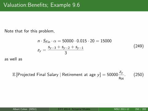
Valuation:Benefits; Example 9.6
Note that for this problem,
n · SFin · α = 50000 · 0.015 · 20 = 15000
zy =sy−3 + sy−2 + sy−1
3
(249)
as well as
E [Projected Final Salary | Retirement at age y ] = 50000zys54
. (250)
Albert Cohen (MSU) STT 455-6: Actuarial Models MSU 2011-12 250 / 283
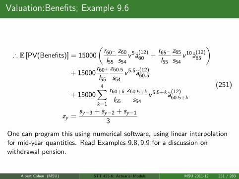
Valuation:Benefits; Example 9.6
∴ E [PV(Benefits)] = 15000
(r60−
l55
z60
s54v 5a
(12)60 +
r65−
l55
z65
s54v 10a
(12)65
)+ 15000
r60+
l55
z60.5
s54v 5.5a
(12)60.5
+ 150004∑
k=1
r60+k
l55
z60.5+k
s54v 5.5+k a
(12)60.5+k
zy =sy−3 + sy−2 + sy−1
3
(251)
One can program this using numerical software, using linear interpolationfor mid-year quantities. Read Examples 9.8, 9.9 for a discussion onwithdrawal pension.
Albert Cohen (MSU) STT 455-6: Actuarial Models MSU 2011-12 251 / 283
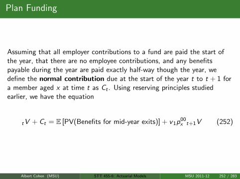
Plan Funding
Assuming that all employer contributions to a fund are paid the start ofthe year, that there are no employee contributions, and any benefitspayable during the year are paid exactly half-way though the year, wedefine the normal contribution due at the start of the year t to t + 1 fora member aged x at time t as Ct . Using reserving principles studiedearlier, we have the equation
tV + Ct = E [PV(Benefits for mid-year exits)] + v 1p00x t+1V (252)
Albert Cohen (MSU) STT 455-6: Actuarial Models MSU 2011-12 252 / 283

Example 9.9
Assume a pension plan with the following valuation methods:
Accrual rate: 1.5%
Final salary plan
Pension based on earnings in the year before age retirement
Normal retirement at age 65
The pension benefit is a life annuity payable monthly in advance
There is no benefit due on death in service
No exits other than by death before normal retirement age
Albert Cohen (MSU) STT 455-6: Actuarial Models MSU 2011-12 253 / 283

Example 9.9
Calculate the value of the accrued pension benefit and normal contributiondue at the start of the year using a projected unit funding (PUC), whereinterest is set at 5% per year, salaries increase at 4% per year and assumea constant mortality µ before and after retirement.
SFin = 50000s64
s49= 50000(1.04)15 = 90047
0V = 0.015 · 20 · SFin · 15p50 · v 15 · a(12)65
= 12994.24 · e−15µ · v 15 · 1
12
∞∑k=0
vk12 e−µ
k12
=12994.24
12e15µ · 1.0515 ·(
1− 12
√1
1.05eµ
)(253)
Albert Cohen (MSU) STT 455-6: Actuarial Models MSU 2011-12 254 / 283
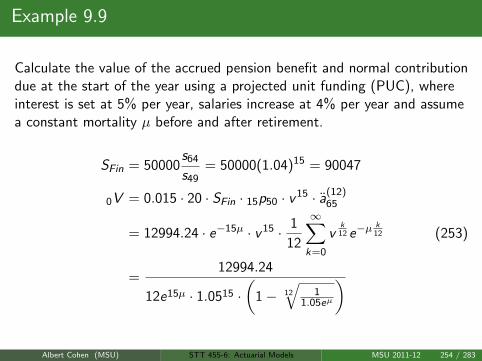
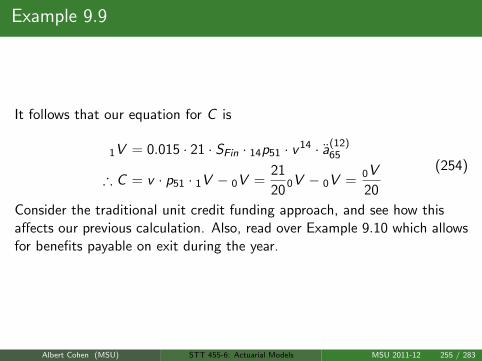
Example 9.9
It follows that our equation for C is
1V = 0.015 · 21 · SFin · 14p51 · v 14 · a(12)65
∴ C = v · p51 · 1V − 0V =21
200V − 0V =
0V
20
(254)
Consider the traditional unit credit funding approach, and see how thisaffects our previous calculation. Also, read over Example 9.10 which allowsfor benefits payable on exit during the year.
Albert Cohen (MSU) STT 455-6: Actuarial Models MSU 2011-12 255 / 283

Homework Questions
HW: 9.1, 9.3, 9.5, 9.7, 9.9, 9.12, 9.13
Albert Cohen (MSU) STT 455-6: Actuarial Models MSU 2011-12 256 / 283
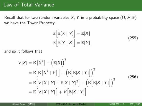
Law of Total Variance
Recall that for two random variables X ,Y in a probability space (Ω,F ,P)we have the Tower Property
E[E[X | Y ]
]= E[X ]
E[E[Y | X ]
]= E[Y ]
(255)
and so it follows that
V [X ] = E[X 2]−(E[X ]
)2
= E[E[X 2 | Y
] ]−(E[E[X | Y ]
])2
= E[V [X | Y ] + E[X | Y ]2
]−(E[E[X | Y ]
])2
= E[V [X | Y ]
]+ V
[E[X | Y ]
](256)
Albert Cohen (MSU) STT 455-6: Actuarial Models MSU 2011-12 257 / 283
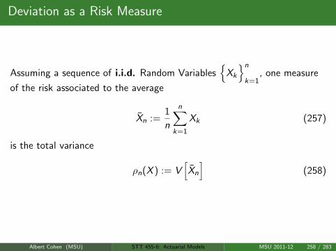
Deviation as a Risk Measure
Assuming a sequence of i.i.d. Random Variables
Xk
n
k=1, one measure
of the risk associated to the average
Xn :=1
n
n∑k=1
Xk (257)
is the total variance
ρn(X ) := V[Xn
](258)
Albert Cohen (MSU) STT 455-6: Actuarial Models MSU 2011-12 258 / 283
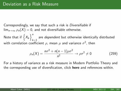
Deviation as a Risk Measure
Correspondingly, we say that such a risk is Diversifiable iflimn→∞ ρn(X ) = 0, and not diversifiable otherwise.
Note that if
Xk
n
k=1are dependent but otherwise identically distrbuted
with correlation coefficient ρ, mean µ and variance σ2, then
ρn(X ) =nσ2 + n(n − 1)ρσ2
n2→ ρσ2 6= 0 (259)
For a history of variance as a risk measure in Modern Portfolio Theory andthe corresponding use of diversfication, click here and references within.
Albert Cohen (MSU) STT 455-6: Actuarial Models MSU 2011-12 259 / 283
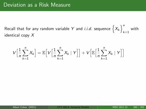
Deviation as a Risk Measure
Recall that for any random variable Y and i.i.d. sequence
Xk
n
k=1with
identical copy X
V[1
n
n∑k=1
Xk
]= E
[V[1
n
n∑k=1
Xk | Y]]
+ V[E[1
n
n∑k=1
Xk | Y]]
=1
nE[V[X | Y
]]+ V
[E[X | Y
]] (260)
It follows that ρn(X )→ 0 as long as V[E[X | Y
]]= 0.
Albert Cohen (MSU) STT 455-6: Actuarial Models MSU 2011-12 260 / 283
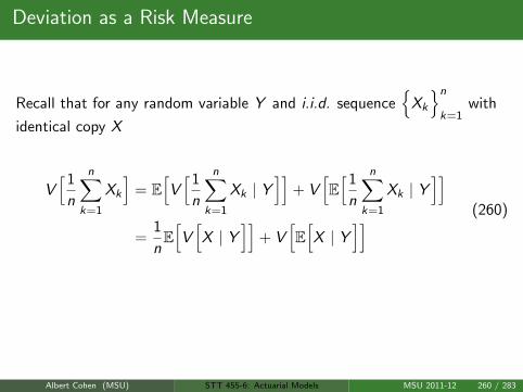
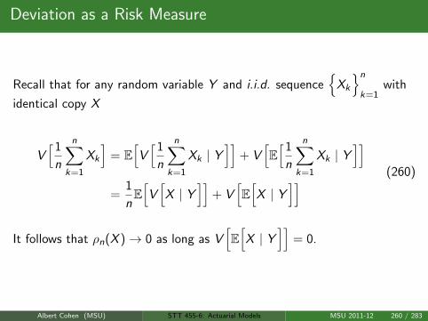
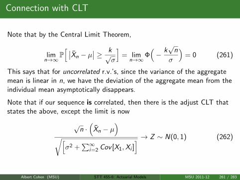
Connection with CLT
Note that by the Central Limit Theorem,
limn→∞
P[ ∣∣Xn − µ
∣∣ ≥ k√σ
]= lim
n→∞Φ(− k√
n
σ
)= 0 (261)
This says that for uncorrelated r.v.’s, since the variance of the aggregatemean is linear in n, we have the deviation of the aggregate mean from theindividual mean asymptotically disappears.
Note that if our sequence is correlated, then there is the adjust CLT thatstates the above, except the limit is now
√n ·(
Xn − µ)
√[σ2 +
∑∞i=2 Cov [X1,Xi ]
] → Z ∼ N(0, 1) (262)
Albert Cohen (MSU) STT 455-6: Actuarial Models MSU 2011-12 261 / 283
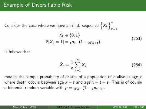
Example of Diversifiable Risk
Consider the case where we have an i.i.d. sequence
Xk
n
k=1
Xk ∈ 0, 1P[Xk = 1] = tpx · (1− spx+t).
(263)
It follows that
Xn =1
n
n∑k=1
Xk (264)
models the sample probability of deaths of a population of n alive at age xwhere death occurs between age x + t and age x + t + s. This is of coursea binomial random variable with p = tpx · (1− spx+t).
Albert Cohen (MSU) STT 455-6: Actuarial Models MSU 2011-12 262 / 283
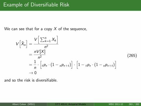
Example of Diversifiable Risk
We can see that for a copy X of the sequence,
V[Xn
]=
V[∑n
k=1 Xk
]n2
=nV [X ]
n2
=1
n·[tpx · (1− spx+t)
]·[1− tpx · (1− spx+t)
]→ 0
(265)
and so the risk is diversifiable.
Albert Cohen (MSU) STT 455-6: Actuarial Models MSU 2011-12 263 / 283
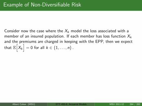
Example of Non-Diversifiable Risk
Consider now the case where the Xk model the loss associated with amember of an insured population. If each member has loss function Xk
and the premiums are charged in keeping with the EPP, then we expect
that E[Xk
]= 0 for all k ∈ 1, . . . , n .
If, however, the forecasted yield rate used is a random variable Y , then ifE[Xk | Y ] 6= 0 we have non-diversifiable risk as
V[Xn
]→ V
[E[X | Y
]]6= 0. (266)
Albert Cohen (MSU) STT 455-6: Actuarial Models MSU 2011-12 264 / 283
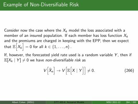

Homework Questions
HW: 10.1, 10.2, 10.3, 10.5, 10.6
Albert Cohen (MSU) STT 455-6: Actuarial Models MSU 2011-12 265 / 283

Reserves
Recall the need for policy values when negative future cash flows wereexpected. In this lecture, we cover the idea of reserves, which is the actualamount of money held by the insurer to cover future liabilities associatedwith contracts.
Albert Cohen (MSU) STT 455-6: Actuarial Models MSU 2011-12 266 / 283

Reserves
The insurer may decide to set aside assets in reserve as equal to the netpremium policy values on a certain (reserve) basis.
For example, consider an n−year term insurance contract issued to a life xwith sum insured S . Since we use the net premium basis to compute fixedpremiums, it follows that
P = SA1x :n
ax :n
⇒ Rt = tV = SA 1x+t:n−t − Pax+t:n−t
= SA1x :n ·
(A 1x+t:n−tA1x :n
−ax+t:n−t
ax :n
) (267)
The cost of setting up, from t − 1 to t, the reserve amount of tV is attime t equal to tV · px+t−1 when valued at time t−
i.e. the proportion of contracts that survive to the end of the year.
Albert Cohen (MSU) STT 455-6: Actuarial Models MSU 2011-12 267 / 283
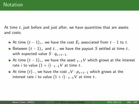
Notation
At time t, just before and just after, we have quantities that are assetsand costs.
At time (t − 1)+, we have the cost Et associated from t − 1 to t.
Between (t − 1)+ and t−, we have the payout S settled at time t−with expected value S · qx+t−1.
At time (t − 1)+, we have the asset t−1V which grows at the interestrate i to value (1 + i) · t−1V at time t−
At time (t)−, we have the cost tV · px+t−1 which grows at theinterest rate i to value (1 + i) · t−1V at time t−
Albert Cohen (MSU) STT 455-6: Actuarial Models MSU 2011-12 268 / 283
Profits
Correspondingly, we can set up an equation for the profit at time t,denoted by Prt :
Prt =(t−1V + P − Et
)(1 + i)− Sqx+t−1 − tVpx+t−1 (268)
The Profit Vector
~Pr :=(
Pr0, . . . ,Prn)
(269)
is comprised of elements that represent the expected profit at the end ofthe year given that the policy is in effect at the start of the year.
Albert Cohen (MSU) STT 455-6: Actuarial Models MSU 2011-12 269 / 283
Profits
The Profit Signature is the the vector ~Π comprised of elements
Πt := t−1pxPrt (270)
that represent the expected profit at the end of the year given that thepolicy was in effect at age x.
Albert Cohen (MSU) STT 455-6: Actuarial Models MSU 2011-12 270 / 283
Profit Measures
Recall that for any set of cash flows Ct , the internal rate of return IRR (ifit uniquely exists) is the interest rate j such that
n∑t=0
Ct
(1 + j)t= 0. (271)
In accordance with the IRR, the insurer may set a minimum hurdle or riskdiscount rate r such that the contract is satisfiably profitable if IRR > r .
Albert Cohen (MSU) STT 455-6: Actuarial Models MSU 2011-12 271 / 283
EPV of Future Profit
If the IRR does not exist, the insurer may seek to measure the profitabilityvia the Net Present Value computed using the risk discount rate:
NPV :=n∑
t=0
Πt
(1 + r)t(272)
Albert Cohen (MSU) STT 455-6: Actuarial Models MSU 2011-12 272 / 283
Profit Margin and DPP
Another measure is the ratio of NPV to E[PV (Premiums)]:
Profit Margin :=NPV
E[PV (Premiums)](273)
as is the discounted payback period DPP:
DPP := min
m :
m∑t=0
Πt
(1 + r)t≥ 0
(274)
which represents the time until the insurer starts to make a profit.
A question naturally arises of how to jointly measure interest risk andprofit. One may even compute the marginal changes in the profit measureswith respect to change in risk discount factor r .
Albert Cohen (MSU) STT 455-6: Actuarial Models MSU 2011-12 273 / 283

Homework Questions
Read Example 11.1
HW: 11.1, 11.3, 11.6, 11.7
Albert Cohen (MSU) STT 455-6: Actuarial Models MSU 2011-12 274 / 283

Equity Linked Insurance
Modern insurance contracts can include some form of guarantee. Theseare known in America as Variable Annuities and Segregated Funds inCanada. The accumulating premiums the policyholder pays is invested onthe policyholder’s behalf. These premiums form the policyholder’s fund,from which regular management charges are deducted by the insurer andpaid into the insurer’s fund to cover expenses and insurance charges.
Albert Cohen (MSU) STT 455-6: Actuarial Models MSU 2011-12 275 / 283

Equity Linked Insurance
On survival to the end of the contract term the benefit may be just thepolicyholder’s fund and no more, or there may be a guaranteed minimummaturity benefit (GMMB). There may also be a guaranteed minimumdeath benefit (GMDB).
There are very real consequences to the differences between financialpricing and actuarial reserving. A short but excellent analysis can be foundin the paper by Bangwon Ko and Elias S. W. Shiu on Financial Pricingand Actuarial Reserving.
Also consider A Heavy Traffic Approach to Modeling Large LifeInsurance Portfolios (Stochastic modeling of actuarial reserve, with Itointegration of a time-changed Brownian Bridge.)
We follow the example set by Shiu and Ko now.
Albert Cohen (MSU) STT 455-6: Actuarial Models MSU 2011-12 276 / 283
Stochastic Actuarial Reserving
Fix a probability space(
Ω,F ,P)
and a standard Brownian motion W
that lives on this space.
Consider now a term contact with term T and let α denote themanagement charges factor along with β representing the policyholder’sparticipation factor.
Furthermore, assume mean and standard deviation parameters (µ, σ)respectively and the corresponding Geometric Brownian Mutual Fund Asset
St = S0eµt+σWt . (275)
Albert Cohen (MSU) STT 455-6: Actuarial Models MSU 2011-12 277 / 283
Stochastic Actuarial Reserving
Using this as the model of the asset returns upon which premiums areinvested, the policyholder wishes to purchase a contract that pays amaturity benefit credited at a rate of return which is the greater of
the customer’s risk discount rate r , where r < µ or
the participation rate of the stock index returns of S .
Symbolically, for a current premium P invested in the , the contractpayout value at maturity is
V (T ) = (1− α)P max
erT , 1 + β
(ST
S0− 1)
. (276)
Albert Cohen (MSU) STT 455-6: Actuarial Models MSU 2011-12 278 / 283
Stochastic Actuarial Reserving
Assume that the policyholder is able to fully participate in the returns fromthe fund (i.e. β = 1.)Then
V (T ) = (1− α)PST
S0+ (1− α)P max
erT −
(ST
S0
), 0
:= V1(T ) + V2(T ).
(277)
Here, V1(T ) is the net premium, or payoff, for investing in the index fundand V2(T ) is the guaranteed option payoff if the index fundunder-performs relative to the risk discount rate r .
How does one reserve to meet the obligations of V2(T ).
Albert Cohen (MSU) STT 455-6: Actuarial Models MSU 2011-12 279 / 283
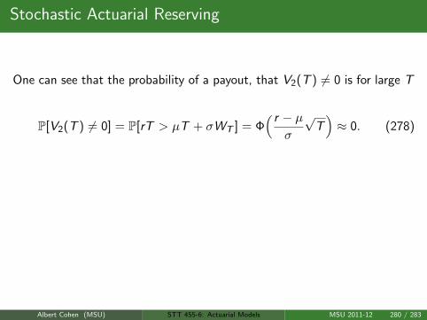
Stochastic Actuarial Reserving
One can see that the probability of a payout, that V2(T ) 6= 0 is for large T
P[V2(T ) 6= 0] = P[rT > µT + σWT ] = Φ( r − µ
σ
√T)≈ 0. (278)
Since it is a low probability event that we have to prepare for a payoutV2(T ) and since we can directly replicate the payoff V1(T ) by initially
purchasing (1−α)PS0
units of the index fund, an actuary may be tempted tonot reserve for the uncertain portion of the guarantee, V2(T ), if thecontract has a relatively long term T .
Is this a wise decision?
Albert Cohen (MSU) STT 455-6: Actuarial Models MSU 2011-12 280 / 283
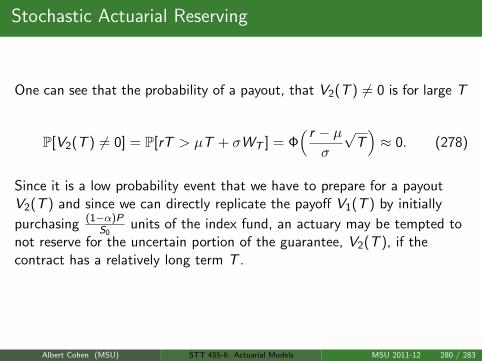
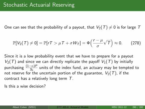
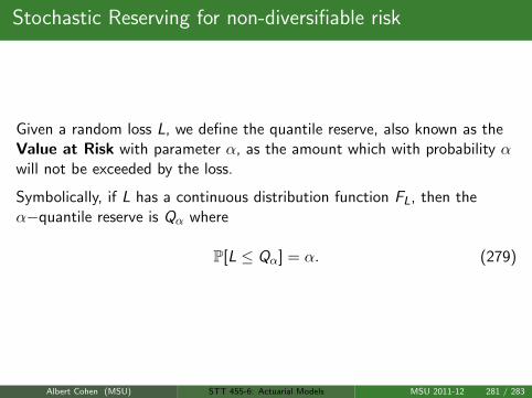
Stochastic Reserving for non-diversifiable risk
Given a random loss L, we define the quantile reserve, also known as theValue at Risk with parameter α, as the amount which with probability αwill not be exceeded by the loss.
Symbolically, if L has a continuous distribution function FL, then theα−quantile reserve is Qα where
P[L ≤ Qα] = α. (279)
Albert Cohen (MSU) STT 455-6: Actuarial Models MSU 2011-12 281 / 283
Stochastic Reserving for non-diversifiable risk
One feature that is missing in VaR is the description of what the loss couldbe if it does exceed the quantile Qα. In this case, the Conditional TailExpectation (CTEα) is defined as
CTEα = E[L | L ≥ Qα]. (280)
A risk manager should not rely on static measures of risk involved with aportfolio of liabilities. Rather, the CTE or VaR reserve should be regularlyupdated to incorporate market information as it arrives. This allowsreserves which are held in less-risky (and possibly more liquid) funds to beinvested higher return and higher risk assets if current market informationdictates that CTE reserves can be reduced.
Albert Cohen (MSU) STT 455-6: Actuarial Models MSU 2011-12 282 / 283

Homework Questions
Read Example 12.1 and Table 12.8
HW: 12.1− 12.5
Albert Cohen (MSU) STT 455-6: Actuarial Models MSU 2011-12 283 / 283