Structured Population Dynamics and Calculus: An

Introduction to Integral Modeling

Joseph Briggs1, Kathryn Dabbs2, Daniel Riser-Espinoza3, Michael Holm4,

Joan Lubben4, Richard Rebarber4 and Brigitte Tenhumberg4,5

1North Carolina State University, Raleigh, NC2University of Tennesse, Knoxville, TN3Swarthmore College, Swarthmore, PA

4Department of Mathematics, University of Nebraska, Lincoln, NE5 School of Biological Sciences, University of Nebraska, Lincoln, NE

Will an exotic species thrive in a new territory? What are the best management options

to eradicate a population (pest species) or to facilitate population recovery (endangered

species)? Population modeling is one method of integrating mathematics and biology in

order to help answer these questions. Most commonly, researchers use population projec-

tion matrices to model a stage structured population. In general, a large number of life

history stages increases model accuracy, but at the cost of increasing parameter uncertainty,

since each non-zero matrix entry needs to be estimated from data. This tradeoff can often be

avoided by using integral projection models which utilize continuous life history functions and

describe a continuous range of stages. In this article we illuminate the differences and simi-

larities between matrix population models and integral population models for single-species

stage structured populations. We illustrate the use of integral models with an application

to Platte thistle, a species in decline in its native environment.

1 Stage Structured Population Models

In a stage structured population model, the individuals are partitioned into demographically

different stage classes. For example, it is natural to divide an insect population into egg,

larva, pupa and adult stages. For mammals, age classes are often used to partition the

1

population. For many plants, the stages can be better described as a continuous function

of stem diameter,m or any other indicator of size. In this case one can either maintain the

continuous stage structure, or partition the continuous range of stages into a finite number

of stages. To do such a discretization effectively, one must ensure that each stage consists of

individuals with comparable growth, survival and fecundity (number of offspring per capita),

because the accuracy of the approximation largely depends on the similarity of individuals

within each stage class. The choice of the stage variable and the breakdown into the stages

is very dependent on the type of population and requires biological intuition. For instance,

fecundity in animals is often influenced by age, while in plants, size is usually a better

measure.

Another basic modeling decision is how time will be treated. Field data is often collected

at regular time intervals, for instance on a yearly or seasonal basis, so it is often easier

and more practical to model time discretely. There is actually a great deal of controversy

about the relative merits of discrete-time versus continuous-time modeling (see, for example,

[6]). In this article we will follow in the tradition of most of the literature on single-species

structured populations, and consider time to be a discrete variable.

A Population Projection Matrix (PPM) model is typically used when both time and stage

structure are discrete, and an integro-difference model, known in this contextx as an Integral

Projection Model (IPM), is used when time is discrete but the stage structure is continuous.

(The continuous-time analogues are ordinary differential equations and integro-differential

or partial differential equations). PPM’s are ubiquitous in ecology, but for many purposes

the IPM might be easier and/or more accurate to use. In Table 2 at the end of this paper

we summarize the similarities between the PPMs and IPMs.

2 Matrix Models

Matrix models were introduced in the mid 1940s, but did not become the dominant paradigm

in ecological population modeling until the 1970s. The modern theory is described in great

detail in Caswell [3], which also contains a good short history of the subject. We summarize

some of this history here. The basic theory of predicting population growth by analyzing

life history parameters such as survival and fecundity can be traced back to Cannan [2] in

1895. Matrix models in particular were developed independently by Bernardelli [1], Lewis

[15], and Leslie [14]. The greatest contributions to the fledgling theory were made by P.H.

Leslie, a physiologist and self-taught mathematician. While working at the Bureau of Animal

Population at Oxford between 1935 and 1968, Leslie sought a way of synthesizing mortality

and fertility data into a single model. In searching for a viable method, he experimented

2

with the idea of modeling a population using matrices. We briefly describe his basic models

in the next section. Leslie then used these models for population description, analysis and

prediction.

Although he was highly regarded and well-connected in the ecology community, Leslie’s

work in matrix modeling initially received little attention. One of the few, and most impor-

tant, contemporaries who did use the matrix model was Leonard Lefkovitch. In [13] he also

implemented a matrix model, but introduced the concept of dividing individuals into classes

based on developmental stage rather than age. This was a great boon to plant ecologists

who began defining stage classes by size rather than age - a change which usually resulted

in better predictions.

As Caswell [3] points out, it took some 25 years for the ecology community to adopt

matrix projection models after Leslie’s influential work. There were two major reasons for

this delay. The ecology community at that time thought of matrix algebra as an advanced

and esoteric subject in mathematics. More importantly, there was a more accessible method,

also contributed by Leslie, called life table analysis. Before the widespread use of comput-

ers, there was no information that a matrix model could provide that a life table could

not. This would change as more sophisticated matrix algebra and computation methods

emerged to convince ecologists the worth of matrix models. For instance, using elementary

linear algebra, one can predict aysmptotic growth rates and stable age distributions from

spectral properties. As one example, the use of eigenvectors facilitated the development of

sensitivity and elasticity analyses, allowing a population manager to determine how small

changes in life history parameters effect the asymptotic population growth rate. This is an

especially important question for ecological models, which typically have high uncertainty.

Sensitivity and elasticity analyses are sometimes used to make recommendations on what

stage class conservation managers should focus on to increase the population growth rate of

an endangered species.

2.1 Transition matrices

To set up a matrix model we start with a population divided into m stage classes. Let t ∈ Nbe time, measured discretely, and let n(t) be the population column vector

n(t) = [n(1, t), n(2, t), . . . , n(m, t)]T ,

where each entry n(i, t) is the number of individuals belonging to class i. A discrete-time

matrix model takes the form

n(t+ 1) = An(t), (1)

3

where A = (ai,j) is the m×m PPM containing the life-history parameters. It is also called

a transition matrix, since it dictates the demographic changes occurring over one time step.

We can write (1) as

n(i, t+ 1) =m∑

j=1

aijn(j, t). (2)

The entries ai,j determine how the number of stage j individuals at time t effect the number

of stage i individuals at time t + 1. This is the form we will generalize when we discuss

integral equations.

In their simplest form, the entries of A are survivorship probabilities and fecundities. For

example, a Leslie matrix is of the form

A =

f1 f2 · · · fm

s1 0 · · · 00 s2 · · · 0... 0

. . . 00 · · · · · · sm

,

where si is the probability that an individual survives from age class i to age class i + 1,

and fi is the fecundity, which is the per capita average number of offspring reaching stage

1 born from mothers of the age class i. The transition matrix has this particular structure

when age is the stage class variable and individuals either move into the next class or die.

In general, entries for the life-history parameters can be in any entry of the m x m matrix.

For any matrix A, it follows from (1) that

n(t) = Atn(0). (3)

The long-term behavior of n(t) is determined by the eigenvalues and eigenvectors of A. We

say that A is non-negative (denoted A > 0) if all of its entries are positive and that A

is primitive if Ak > 0 for some k ∈ N . This second condition is equivalent to every stage

class having a descendent in every other stage class at some time step in the future. PPMs

are generally positive and primitve, thus the following Perron-Frobenius Theorem (see for

instance [19]) is extremely useful:

Theorem 2.1. Let A be a square, non-negative, primitive matrix. Then A has an eigen-

value, λ, which satisfies:

1. λ is real and λ > 0,

2. λ has right and left eigenvectors whose components are strictly positive,

4

3. λ > |λ| for any eigenvalue |λ| 6= λ,

4. λ has algebraic and geometric multiplicity 1.

Assume that A is primitive. Letting ‖n‖ denote the `1 norm, i.e.

‖n‖ = |n1|+ |n2|+ . . . |nm|, (4)

and letting the dominant (i.e. greatest magnitude) eigenvalue of A be given by λ, and its

associated eigenvector by v, then

limt→∞

‖n(t+ 1)‖‖n(t)‖

= λ, limt→∞

n(t)

‖n(t)‖= v. (5)

Thus λ is the asymptotic growth rate, and v is the stable age structure of the population.

2.2 Problems with stage discretization

To use a population projection matrix model, the population needs to be decomposed into

a finite number of discrete stage classes that are not necessarily reflective of the true pop-

ulation structure. Easterling [7] and Easterling et al. [8] showed that erroneous predictions

of the asymptotic growth rate occur if the stage classes are chosen in a way which is not

biologically realistic. Fortunately it is often possible to decompose a particular population in

a biologically sensible fashion. Vandermeer [20] and Moloney [16] crafted algorithms to min-

imize errors associated with choosing class boundaries. While such algorithms help to derive

more reasonable matrices they cannot altogether eliminate the sampling and distribution

errors associated with discretization [3].

With or without a sensible decomposition of the population into stages, there is also the

problem that in a matrix model individuals of a given stage class are treated as though they

are identical through every time step. That is, two individuals starting in the same class

will always have the same probability of transitioning into a different stage class at every

time step in the future, which is not necessarily the case for real populations. There is also

a crucial tradeoff between biological realism and parameter uncertainty when choosing the

number of stage classes. A model will lose realism as the number of stage classes diminishes

because increasingly dissimilar individuals are grouped together. Alternatively, if too many

stage classes are used, the model becomes overburdened with new parameters and there is

increased parameter uncertainty because fewer and fewer data points are used to estimate

life-history parameters. Furthermore, sensitivity and elasticity analyses both have been

shown to be affected by changes in stage class division [8].

5

3 Integral Projection Models

An alternate approach to discretizing continuous variables like size is to use integral projec-

tion models. A class of IPMs is introduced in Easterling [7], Easterling et al [8] and Ellner

and Rees [9]. These models retain much of the analytical machinery which makes the matrix

model appealing, while allowing for a continuous range of stages. In [7, 8] it is shown how

to construct such an integral projection model, using continuous stage classes and discrete

time, and provided sensitivity and elasticity formulas comparable to those of matrix models.

In [9] an IPM analogue of the Perron-Frobenius Theorem is given. In particular, there are

readily checked conditions under which such a model has an asymptotic growth rate which

is the dominant eigenvalue of an operator whose associated eigenvector is the asymptotic

stable population distribution.

Just as ecologists were slow to adopt matrix models, integral models are not yet widely

used. Stage structured IPMs of the type considered in this paper appeared in the scientific

literature around ten years ago, and can be found in [4, 5, 7, 8, 9, 10, 17, 18]. There is a

large literature on integral models for spatial spread of a population, see for instance Kot,

et al. [11, 12]. In this case the kernel for the integral operator can be very different than for

the integral projection models discussed in this paper. For instance, the kernel describing

spatial spread will typically have a support which is not finite, and might not even be square

integrable; this makes the spectral analysis, and hence the asymptotic analysis, much more

difficult. The integral operators discussed in this paper are compact operators, which have

many properties that are similar to those for matrices.

3.1 Continuous stage structure and integral operators

Let n(x, t) be the population distribution as a function of the stage x at time t. For example,

x ∈ [ms,Ms] could be the size of the individual, where ms is the minimum size, and Ms is

the maximum size. The analogue of the matrix entries (ai,j) (for i, j ∈ 0, 1, . . .m) is

a projection kernel k(y, x) (for y, x ∈ [ms,Ms]), and the role of the matrix multiplication

operation is analogous to an integral operator. The analogue of (2) is

n(y, t+ 1) =

∫ Ms

ms

k(y, x)n(x, t)dx. (6)

In particular, the kernel determines how the distribution of stage x individuals at time t

moves to the distribution of stage y individuals at time t+ 1, in much the same way that in

(2) the (i, j)th entry of a projection matrix determines how an individual in stage j at time t

moves to state i at time t+ 1. The kernel is determined by statistically derived functions for

6

survival, growth and fecundity. An advantage of the integral approach is that data over the

entire distribution can be used to estimate the parameters of the functions, thus minimizing

the parameter uncertainty. In contrast, in matrix models transitions between life history

stages are estimated for subsets of data.

The stage variable x does not have to be a scalar, but the range of stage variables should

be a compact metric space. For example, for a plant, a stage could contain information on

both size and quality. In cases like this where x is not a scalar, the Riemann integration over

a subset of R will be replaced by more general integration over a product space; see Ellner

and Rees [9] for such an example.

Integral equations such as (6) can be analyzed in much the same way as matrix-based

models of the form (1). Consider the L1-norm

‖f‖ :=

∫ Ms

ms

|f(x)|dx,

which is analogous to (4). The space

L1(ms,Ms) = f : (ms,Ms)→ R | ‖f‖ <∞

is well-known to be a compact metric space. For every t > 0, the population distribution

n(t, ·) is in L1(ms,Ms), and the total population is ‖n(t)‖. Hence L1(ms,Ms) plays the same

role in an IPM that Rm (with norm (4)) plays in a PPM.

For a population distribution n(x, t), it is sometimes useful to distinguish between the

function n(x, t) of two variables and the L1(ms,Ms)-valued function of a single variable

n(t) = n(·, t); we refer to n(t) as a “vector” in L1(ms,Ms). Define the operator A :

L1(ms,Ms)→ L1(ms,Ms) by

(Av)(·) :=

∫ Ms

ms

k(·, x)v(x)dx.

It is not hard to show that A is bounded on L1(Ω). Then (6) is equivalent to

n(t+ 1) = An(t), (7)

which is analogous to (1).

Ellner and Rees [9] show that for a large class of kernels k, the integral operator A satisfies

the conclusions of the Perron-Frobenius Theorem, so for these operators there is a dominant

real eigenvalue λ which is the asymptotic growth rate, and an associated eigenvector v

7

which is the stable stage distribution. In the operator case the eigenvectors are functions in

L1(ms,Ms), rather than vectors in Rm. In this case the first equation in (5) holds, and the

second equation holds if the convergence is interpreted as L1(ms,Ms) convergence.

3.2 The kernel

To construct the kernel, we construct a growth and survival function p(y, x) and a fecundity

function f(y, x), and let

k(y, x) = p(y, x) + f(y, x).

Here p(y, x) is the probability that an individual of size x will survive and grow to be an

individual of size y in one time step. The function f(y, x) is the number of offspring of size

y that an individual of size x will produce in one time step. Typically p(y, x) can be written

as s1(x)g(y, x), where s1(x) is the probability of survival for a size x individual to the next

time step and the growth function g(y, x) is the probability that an individual of size x will

be of size y at the next time step. The growth function can describe both the probability

of growing to a larger size and the probability of shrinking to a smaller size. The fecundity

function f(y, x) is typically written as f1(x)f2(y, x), where f1(x) is the average number of

offspring of parents of size x, and f2(y, x) is the probability that the offspring of a size x

parent are size y at the next time step. We should point out that the fecundity function

allows for the possibility of a seedling or newborn moving, in one time step, to a large size,

but in practice the probability of this happening will virtually be zero.

The function s1(x), g(y, x), f1(x), and f2(y, x) are estimated using from the data using

standard statistical methods. For instance, logistic regression analysis can be used to describe

survival as a function of size. For more details on the appropriate statistical models for

integral projection models see Easterling et al. [8], Ellner and Rees [9], and Rose et al. [18].

3.2.1 Estimating the kernel for Platte thistle

We now show how a specific model is constructed, using a version of the model for Platte

thistle (Cirsium canescens) found in Rose et. al. [18], modified to ignore effects of herbaceous

predators. Platte thistle is an indigenous perennial plant in the midgrass sand prairies of

central North America. It is strictly monocarpic, meaning that plants die after reproducing,

so the flowering probability will need to be incorporated into the kernel. It is in decline in

its native environment, possibly due to a biocontrol aagent introduced to manage a different

invasive thistle. In this model, we use the root crown diameter x as the continuous class

variable. The survival probability s(x) and flowering probability fp(x) respectively, are given

8

in Table 1. Since the Platte thistle is monocarpic, we have to include the probability of not

flowering, which is 1− fp(x), so s1(x) = s(x)(1− fp(x)). Also given in Table 1 is the average

growth µ(x) and the variance of growth σ(x) (which in this case is constant). The growth

function g(y, x) is a normal distribution in the variable y, with mean µ(x) and variance σ(x).

We now turn our attention to the fecundity term of the kernel, f(y, x). To best illustrate

the basic concepts, we simplify the model by ignoring the effects of herbivores on fecundity,

and the possible slight effect of maternal size on offspring size. In order to reproduce, a plant

must survive, and it must also flower. Each plant will produce seeds, and these seeds must

germinate for an offspring to be included in the next population count. The number of seeds

S(x) produced by each plant is an exponential function of size x. The average germination

probability Pe, also known as the recruitment probability, is constant - later we will consider

the case where this is not constant. Finally, we also need a distribution of the offspring sizes

J(y); we assume here that this is a normal distribution with constant mean µf and variance

σf . Therefore,

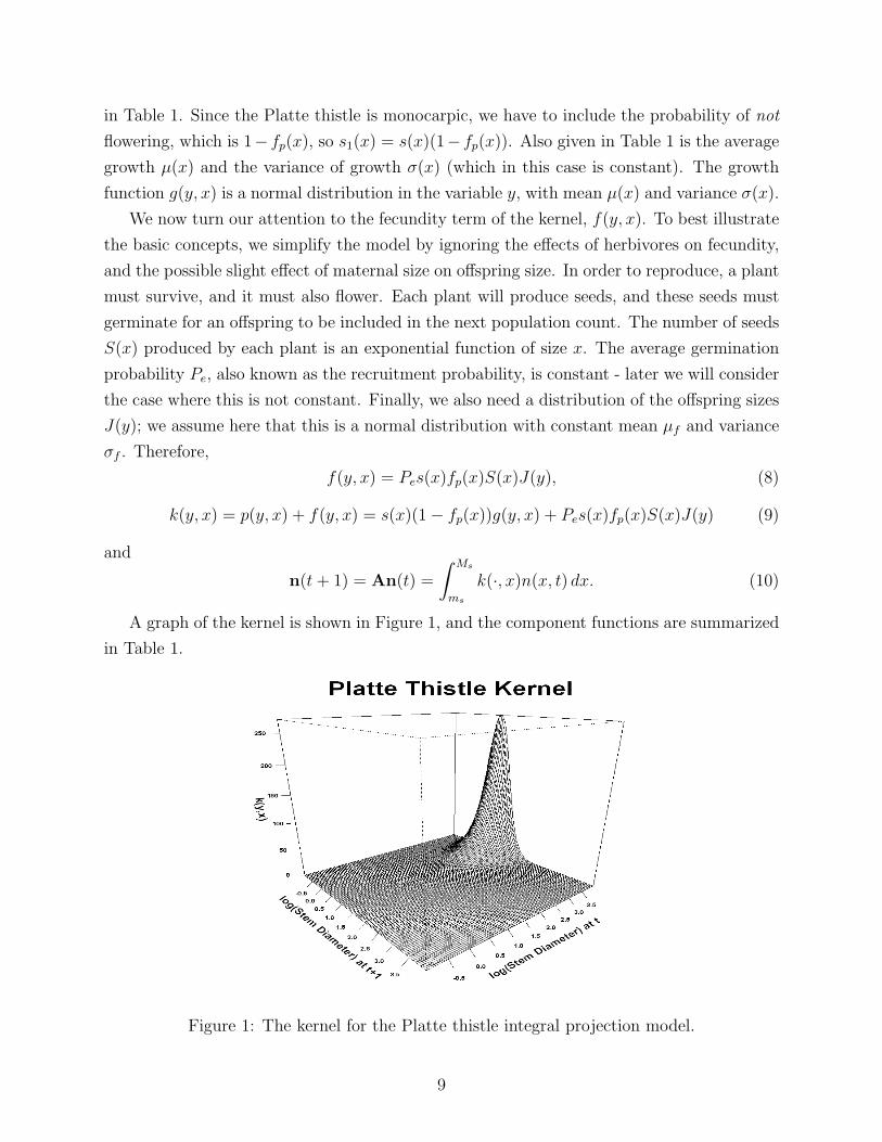
f(y, x) = Pes(x)fp(x)S(x)J(y), (8)

k(y, x) = p(y, x) + f(y, x) = s(x)(1− fp(x))g(y, x) + Pes(x)fp(x)S(x)J(y) (9)

and

n(t+ 1) = An(t) =

∫ Ms

ms

k(·, x)n(x, t) dx. (10)

A graph of the kernel is shown in Figure 1, and the component functions are summarized

in Table 1.

Figure 1: The kernel for the Platte thistle integral projection model.

9

Demography Equation

Survival s(x) = e−0.62+0.85x

(1+e−0.62+0.85x)

Flowering Probability fp(x) = e−10.22+4.25x

(1+e−10.22+4.25x)

g(x,y) = Normal Distribution

Growth Distribution with σ(x)2 = 0.19

and µ(x) = 0.83 + 0.69x

Individual Seed Set S(x) = e0.37+2.02x

J(y) = Normal Distribution

Juvenile Size Distribution with σ2f = 0.17

and µf = 0.75

Germination Probability Pe = .067 density independent

or

Pe = ST (t)−0.33 density dependent

where ST (t) is the total seed set

Table 1: Life History Functions for Platte Thistle [18].

3.3 Numerical solution of the integro-difference equation

Analytic evaluation of the integral operator is difficult if not impossible to perform. Thus,

we will use numerical integration to obtain an estimate of the population. A conceptually

easy and relatively accurate method is the midpoint rule. Let N be the number of equally

sized intervals, and let xj be the midpoints of the intervals. Then

(An)(y, t) =

∫ Ms

ms

k(y, x)n(x, t)dx ≈ Ms −ms

N

N∑j=1

k(y, xj)n(xj, t). (11)

Let

ai,j =Ms −ms

Nk(xi, xj) for i, j = 1, 2, . . . N, AN = (ai,j)

10

and

nN(t) = [n(x1, t), n(x2), . . . n(xN , t)]T .

Then nN(t) is a discrete approximation of n(x, t), AN is a discrete approximation of the

integral operator A, and

ANnN =Ms −ms

N

N∑j=1

k(xi, xj)n(xj, t).

Since k(x, y) is continuous, the Riemann sum uniformly approximates the integral as N →∞. Hence the integrodifference equation n(t + t) = An(t) can be approximated at the

midpoints xj by nN(t+ 1) = ANnN(t).

This matrix model can be analyzed much like a traditional matrix model. Since the

dominant eigenvalue of AN converges to the dominant eigenvalue of A as N → ∞ (Ellner

and Rees [9], Easterling [7]), the long term growth rate is easily estimated. Figure 2 shows

this convergence of λN to λ = 1.325 as N increases. The leading eigenvalue of A5 is 1.332, so

we see that fairly small dimensional approximations of A lead to very good approximations

of the long-term growth of the system.

We should emphasize the difference between a PPM and the matrix model obtained from

the IPM. In the former every nonzero entry is estimated directly; a large matrix of this type is

not intended to approximate the IPM. In the latter, the life history functions are estimated,

giving rise to a kernel, and this kernel is used to obtain a matrix which does approximate

the IPM for large N .

We now turn to the stable size distribution, that is, the limiting distribution given by the

second equation in (5). This can be found by approximating the leading eigenvector of A,

and normalizing it so that it has L1(ms,Ms) norm of 1. This eigenvector, which is shown in

Figure 3, is uniformly approximated by the normalized leading eigenvector of AN for large

N (see Ellner and Rees [9]).

3.4 Density dependence

In the Platte thistle model above, we made the simplifying assumption that the average

germination probability, Pe, is constant, and obtained a density independent model. By

“density independence” we mean that n(t+1) is a linear function of n(t), or equivalently, the

operator A does not depend upon n(t). The growth rate of 1.332 we obtain from this model

is unrealistically large, so we consider a more realistic model where Pe is dependent upon

ST (t), the total number of seeds produced. Since the number of seeds produced depends

11

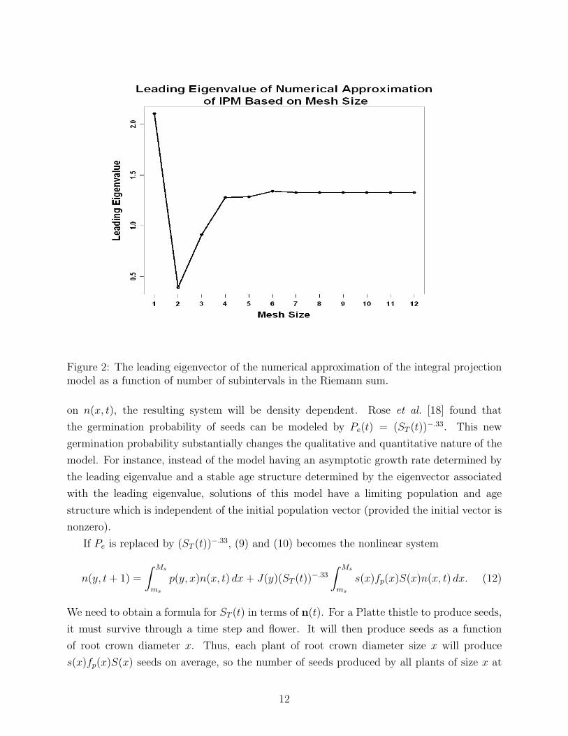
Figure 2: The leading eigenvector of the numerical approximation of the integral projectionmodel as a function of number of subintervals in the Riemann sum.

on n(x, t), the resulting system will be density dependent. Rose et al. [18] found that

the germination probability of seeds can be modeled by Pe(t) = (ST (t))−.33. This new

germination probability substantially changes the qualitative and quantitative nature of the

model. For instance, instead of the model having an asymptotic growth rate determined by

the leading eigenvalue and a stable age structure determined by the eigenvector associated

with the leading eigenvalue, solutions of this model have a limiting population and age

structure which is independent of the initial population vector (provided the initial vector is

nonzero).

If Pe is replaced by (ST (t))−.33, (9) and (10) becomes the nonlinear system

n(y, t+ 1) =

∫ Ms

ms

p(y, x)n(x, t) dx+ J(y)(ST (t))−.33

∫ Ms

ms

s(x)fp(x)S(x)n(x, t) dx. (12)

We need to obtain a formula for ST (t) in terms of n(t). For a Platte thistle to produce seeds,

it must survive through a time step and flower. It will then produce seeds as a function

of root crown diameter x. Thus, each plant of root crown diameter size x will produce

s(x)fp(x)S(x) seeds on average, so the number of seeds produced by all plants of size x at

12

Figure 3: Stable state population densities of Platte thistle.

time t is s(x)fp(x)S(x)n(x, t). Hence the total number of seeds at time t is

ST (t) =

∫ Ms

ms

s(x)fp(x)S(x)n(x, t)dx. (13)

Therefore, (12) becomes

n(y, t+ 1) =

∫ Ms

ms

p(y, x)n(x, t) dx+ J(y)(ST (t)).67. (14)

It is possible to prove that the solutions n(·, t) of (14) converges in L1(ms,Ms) as t→∞,

and that the limit is independent of the initial population vector (provided that the initial

population vector is nonzero). We denote the limit by w(·), and the normalized limit (the

second equation in (5)) by v(·). This latter vector is the stable age distribution for this

system, and is shown in Figure 3. It follows from the Dominated Convergence Theorem that

the total population N(t) = ‖n(·, t)‖ converges to ‖w‖ as t→∞, and that the limiting total

population is independent of the initial population vector. This is illustrated in Figure 4,

where the total population as a function of time is shown for five different initial conditions.

13

Figure 4: Circles indicate every stage of the population contains 1000 individuals; trianglesindicate the population consists of 10,000 individuals of sizes 0 to 1.1 mm only; X’s indicatethe population consists of 1000 individuals of sizes 54.45-55 mm only; plusses indicate apopulation of 500,000 individuals of sizes 0-.55 mm; and diamonds indicate a population of10,000 consisting only of sizes 54.45-55 mm.

To clarify the limiting behavior of the solutions to this nonlinear system, let P0 =

limt→∞(ST (t))−.33 and take the limit as t → ∞, in equation (12) to see that w(·) satis-

fies

w(y) =

∫ Ms

ms

p(y, x)w(x) dx+ P0J(y)

∫ Ms

ms

s(x)fp(x)S(x)w(x) dx. (15)

Define A0 and A1 by

(A0ϕ)(y) =

∫ Ms

ms

p(y, x)ϕ(x) dx for ϕ ∈ L1(ms,Ms),

(A1ϕ)(y) =

∫ Ms

ms

p(y, x)ϕ(x) dx+ P0J(y)

∫ Ms

ms

s(x)fp(x)S(x)ϕ(x) dx for ϕ ∈ L1(ms,Ms).

It follows from (15) that A1 has an eigenvalue of 1 and associated eigenvector w = w(·).Rather than taking a limit in order to get P0, which can be time-consuming and inaccurate,

14

it can be shown that (letting I denote the identity operator)

P0 =

(∫ Ms

ms

s(x)fp(x)S(x)[(I −A0)−1J ](x) dx

).

To evaluate this, the operator A0 and hence (I−A0)−1 and (I−A0)

−1J , can be approximated

as in section 3.3. Once we have P0, the limiting population distribution v(·) is the normalized

eigenvector of A1.

4 Further Reading

For further information on using matrices in the biological sciences, Caswell [3] gives a thor-

ough treatment of the subject. For more information concerning integro-difference equations

Eastering et al. [8] is a good introduction with the theoretical footings of the method con-

tained in the appendices of Ellner and Rees [9].

15

Pop

ula

tion

Pro

ject

ion

Mat

rix

Inte

gral

Pro

ject

ion

Model

num

ber

ofnu

mbe

rof

vect

oren

try

n(i

,t)

indi

vidu

als

inst

age

cont

inuo

usn

(y,t

)or∫ y 1 y

0n

(y,t

)dy

indi

vidu

als

expe

cted

clas

si

atti

me

tfu

ncti

onbe

twee

nsi

zes

y 0an

dy 1

stag

edi

stri

buti

onco

ntin

uous

stag

edi

stri

buti

onst

ate

vect

orn

(t)

=[n

(1,t

),···,

n(m

,t)]

T∈

Rm

ofpo

pula

tion

stat

en

(·,t)∈

L1(m

s,M

s)

ofpo

pula

tion

atti

me

tfu

ncti

onat

tim

et

prob

abili

tyof

anpr

obab

ility

prob

abili

tyan

prob

abili

typ

ijin

divi

dual

dens

ity

p(y

,x)

or∫ y 1 y

0p(y

,x)d

yin

divi

dual

ofsi

zex

tran

siti

onin

gfu

ncti

onw

illgr

owan

dsu

rviv

efr

omcl

ass

jto

ito

asi

zebe

twee

ny 0

and

y 1

num

ber

ofnu

mbe

rof

new

born

sfu

ncti

onf i

jne

wbo

rns

size

ifu

ncti

onf

(y,x

)or∫ y 1 y

0f

(y,x

)dy

betw

een

size

sy 0

and

y 1

from

pare

nts

size

jfr

ompa

rent

sof

size

x

the

ijth

entr

ym

atri

xen

try

kij

=p

ij+

f ij

ofth

efu

ncti

onk(y

,x)

=p(y

,x)

+f

(y,x

)ke

rnel

tran

siti

onm

atri

x

inte

gral

mat

rix

A=

[kij

]op

erat

or(A

v)(

y)

=∫ M s m

sk(y

,x)v

(x)d

x

disc

rete

mat

rix

indi

ces

cont

inuo

usva

riab

les

stag

ej∼

tan

di∼

t+

1as

soci

ated

wit

hst

age

x∼

tan

dy∼

t+

1as

soci

ated

wit

hva

riab

les

tim

et

and

tim

et+

1va

riab

les

tim

et

and

tim

et+

1

diffe

renc

ein

tegr

aleq

uati

onn

(j,t

+1)

=∑ m i=

1k

ijn

(i,t

)eq

uati

onn

(y,t

+1)

=∫ M s 0

k(y

,x)n

(x,t

)dx

vect

orm

atri

xop

erat

orfo

rm~n

(t+

1)=

A~n

(t)

mul

tipl

icat

ion

form

~n(t

+1)

=A

~n(t

)in

tegr

atio

n

Tab

le2:

Com

par

ison

ofM

atri

xan

dIn

tegr

alM

odel

s

16

Acknowledgements

This work was supported by NSF REU Site Grant 0354008. RR was supported in part

by NSF Grant 0606857. We would like to thank Professor Stephen Ellner (Cornell Univer-

sity, Department of Ecology and Evolution) who suggested that we write this expository

description of integral projection models.

References

[1] H. Bernardelli, Population waves, J. Burma Research Society 31 (1941) 1-18.

[2] E. Cannan, The probability of a cessation of the growth of population in England and

Wales during the next century, Economic Journal 20 (1895) 505-515.

[3] H. Caswell, Matrix Population Models, Construction, Analysis, and Interpretation, Sec-

ond Addition, Sinauer Associates, Inc., Sunderland, MA, 2001.

[4] D.Z. Childs, M. Rees, K. E. Rose, P. J. Grubb, and S. P. Ellner, Evolution of complex

flowering strategies: an age- and size- structured integral projection model, Proc. Roy.

Soc. London B 270 (2003) 1829-1838.

[5] D.Z. Childs, M. Rees, K. E. Rose, P. J. Grubb, and S. P. Ellner, Evolution of size-

dependent flowering in a variable environment: construction and analysis of a stochastic

integral projection model, Proc. Roy. Soc. London B 271 (2004) 425-434.

[6] B. Deng, The Time Invariance Principle, the absence of ecological chaos, and a funda-

mental pitfall of discrete modeling, Ecological Modelling, 215 (2008) 287-292.

[7] M.R. Easterling, The integral projection model: theory, analysis and application, PhD

disseration, North Carolina State University, Raleigh, NC, (1998).

[8] M.R. Easterling, S. P. Ellner, and P. M. Dixon, Size-specific sensitivity: applying a new

structured population model, Ecology 81 (2000) 694-708.

[9] S.P. Ellner and M. Rees, Integral Projection Models for Species with Complex Demog-

raphy, American Naturalist 167 (2006) 410-428.

[10] S.P. Ellner and M. Rees, Stochastic stable population growth in integral projection

models: theory and application, J. Math. Biology 54 (2007) 227-256.

17

[11] M. Kot, Discrete-time traveling waves: ecological examples, J. Math. Biology, 30 (1992)

413-436.

[12] M. Kot, M.A. Lewis, and P. van den Driessche, Dispersal data and the spread of invading

organisms, Ecology 77 (1996) 2027-2042.

[13] L.P. Lefkovitch, The study of population growth in organizms grouped by stages, Bio-

metrics 21 (1965) 1-18.

[14] P.H. Leslie, On the use of matrices in certain population mathematics, Biometrika 33

(1945) 183-212.

[15] E.G. Lewis, On the generation and growth of a population, Sankhya: The Indian Journal

of Statistics 6 (1942) 93-96.

[16] K.A. Moloney, A generalized algorithm for determining category size, Oecologia 69

(1986) 176-180.

[17] M. Rees and K.E. Rose, Evolution of flowering strategies in Oenothera glazioviana: an

integral projection model approach, Proc. Roy. Soc. London B 269 (2002) 1509-1515.

[18] K.E. Rose, S.M. Louda, and M. Rees, Demographic and evolutionary impacts of native

and invasive insect herbivores on Cirsium canescens, Ecology 86 (2005) 453-465.

[19] E. Seneta, Non-negative Matrices and Markov Chains, Springer-Verlag, New York, NY,

1981.

[20] J. Vandermeer, Choosing category size in a stage projection matrix, Oecologia 32 (1978)

79-84.

18