Fabien S. Godeferd1

LMFA UMR 5509 CNRS,�Ecole centrale de Lyon,

Universit�e de Lyon,�Ecully 69134, France

e-mail: fabien.godeferd@ec-lyon.fr

Fr�ed�eric MoisyFAST UMR 7608 CNRS,

Universit�e Paris-Sud,

Orsay 91405, France

e-mail: frederic.moisy@fast.u-psud.fr

Structure and Dynamics ofRotating Turbulence: A Reviewof Recent Experimental andNumerical ResultsRotating turbulence is a fundamental phenomenon appearing in several geophysical andindustrial applications. Its study benefited from major advances in the recent years, butalso raised new questions. We review recent results for rotating turbulence, from severalnumerical and experimental researches, and in relation with theory and models, mostlyfor homogeneous flows. We observe a convergence in the statistical description of rotat-ing turbulence from the advent of modern experimental techniques and computationalpower that allows to investigate the structure and dynamics of rotating flows at similarparameters and with similar description levels. The improved picture about the aniso-tropization mechanisms, however, reveals subtle differences in the flow conditions,including its generation and boundary conditions, which lead to separate points of viewabout the role of linear mechanisms—the Coriolis force and inertial waves—comparedwith more complex nonlinear triadic interactions. This is discussed in relation with themost recent diagnostic of dynamical equations in physical and spectral space.[DOI: 10.1115/1.4029006]

1 Introduction

Among a wide range of distortions that can affect the propertiesof turbulent flows, rotation is widely studied from its presence inseveral contexts, from astrophysical and geophysical to industrialflows. On Earth or on planets with atmospheres as Jupiter, thescales are such that the flows are essentially turbulent, and theCoriolis force induced by rotation about the polar axis is responsi-ble for a complex dynamics without which strong coherent struc-tures would not exist: instances are cyclones on the Earth or thegreat red spot in the Jovian atmosphere. Various rotation ratesmay be encountered now that several extrasolar planets have beenfound (the variability of rotation rates in their host stars isreported, e.g., in Ref. [1]), and this justifies parametric investiga-tions that help to link orbital disturbances to the internal behaviorof planetary flows, partly driven by solid body rotation. In giantplanets such as Jupiter, the atmospheric circulation is stronglyaffected by rotation, in addition to density effects, with variableintensities found in extrasolar planets [2]. Back on Earth, theatmosphere has a dynamics strongly related to the diurnal cycle,which is also the case of flows in the ocean, although the scalesinvolved in atmospheric flow dynamics may be different from theoceanic ones.

At human level, rotation also modifies the flow dynamicsthrough the Coriolis force. This is encountered in turbomachinery,especially in large-scale energy producing water or wind turbines[3], and in compressors or turbines of turbofan reactors wherevery large rotation rates are present, up to 105 rpm. In these inter-blade flows, however, pressure and compressibility effects may bedominant over rotation ones. In industrial flows, rotation is there-fore also in competition with finite-size effects and the presenceof other distortions which may be of large amplitude; for instance,walls or solid bodies introduce velocity gradients that oftenredistribute energy more efficiently, or faster, than Coriolis force

does. Density variations can also often be strong, and introducebuoyancy forces that interact with the Coriolis force [4]. Therelies an important specificity of rotating flows, in that the Coriolisforce does no work, unlike other kinds of body forces, Lorentz,buoyancy, etc., and is not a production term in the same sense asvelocity-gradient-related production in the energy balance equa-tion [5]. Rotation, however, does redistribute energy in its ownspecific way, which is not the object of a wide consensus, con-cerning its modeling. This focus particularly questions the linearor nonlinear nature of the effect of rotation on turbulent flows, anda univocal answer is not yet available, since an accurate analysisof the different timescales and topological effects involved in thedynamics is required, all effects that may drive rotating flows todifferent regimes. Among the parameters to account for thiscomplexity, the flow regime is utterly important, characterized bythe Rossby number Ro¼U/(2X‘) and the Reynolds numberRe¼U‘/� – U is a velocity scale associated with an integrallength scale of turbulence ‘. One may also list other effects, suchas confinement, slight asymmetries or perturbations—e.g., biasesinduced by periodic boundary conditions in simulations— and theinitial conditions.

In the presence of solid walls, rotation can become a productionterm, and different kinds of boundary layers appear depending onthe orientation of the wall: Ekman layers develop along horizontalboundaries when the orientation of rotation is vertical—which weare going to assume from now on, with z the vertical direction—whereas Stewartson layers develop on vertical boundaries [6,7].The Ekman number E¼ �/(2XL2)—rotation rate X, container sizeL, kinematic viscosity �—is used to characterize the thickness ofthese layers, being for instance LE1=2 for the Ekman layers. Weshall focus in this review on the dynamics of rotating turbulenceaway from solid boundaries, assuming negligible transport phe-nomena linked with the presence of remote walls, such as Ekmanpumping. In addition, the homogeneity assumption is valid only ifthe integral scale ‘ is significantly smaller than the size of the fluiddomain L.

The dynamics of homogeneous rotating turbulence is thereforea rather intricate issue, which has been tackled in different ways,

1Corresponding author.Manuscript received January 10, 2014; final manuscript received October 30,

2014; published online January 15, 2015. Assoc. Editor: Herman J. H. Clercx.

Applied Mechanics Reviews MAY 2015, Vol. 67 / 030802-1Copyright VC 2015 by ASME

Downloaded From: http://appliedmechanicsreviews.asmedigitalcollection.asme.org/ on 01/16/2015 Terms of Use: http://asme.org/terms

with models ranging from simple to sophisticated, starting fromlinear approximations and extending to full nonlinear modeling ofthird-order velocity statistics. The famed Taylor–Proudman theo-rem applies to rapidly rotating flows [6,8,9]: whenever forcingimposes an external timescale, the neglect of velocity derivativesalong the rotation axis is permitted. Fluid columns are thereforeset in motion like solid bodies, and the flow may be considered tobe two-dimensional, although the vertical velocity component notnecessarily vanishes, and can behave as a convected scalar. Thedegree to which homogeneous rotating turbulence becomes natu-rally two-dimensional is debated and, as mentioned, depends onseveral factors. Considering freely decaying turbulence initiatedwith given conditions, the Taylor–Proudman theorem does notapply to explain the two-dimensionalization of the flow, whichalso strongly depends on the value of the Rossby number Ro.When Ro� 1, the turbulent flow evolves much faster than thetimescale over which rotation can be felt, and is thus unperturbedby rotation. In statistically steady rotating turbulence, a low-enough Rossby number is required for rotation to affect signifi-cantly the flow dynamics. In freely decaying turbulence, or inspatially evolving turbulent flows—e.g., in wind tunnel experi-ments, or the spatial diffusion of a turbulent patch—the Rossbynumber is required to decrease to values below unity for rotationto effectively modify the flow dynamics. At low values, Ro< 0.1or below, the rotation timescale 1/X is small enough for the Corio-lis force to have time to change a turbulent structure whichevolves over a timescale ‘/U, and it progressively affects smallerscales when the Rossby number decreases. Thus, consideringvery large Reynolds number Re, or infinite, the asymptotic limitRo ! 0 is an interesting one, considered mathematically inRef. [10]. For more realistic values, at finite Reynolds number, theCoriolis force affects differently large and small scales. The com-parison of the Coriolis timescale to that of turbulent structures ofa given size led Zeman [11] to introduce the scale lX at which theinertial and eddy turnover times are equal. The Zeman scale maytherefore be considered as a demarcation value above which largescales are affected by rotation while the small scales below lXmay recover isotropic turbulence properties.

Different regimes are illustrated as a function of Rossby andReynolds number in the schematic of Fig. 1. Inertial waves areobserved in the linear, low Reynolds number regime, whereasweak interactions are expected to occur in the wave turbulenceregime encountered asymptotically at vanishing Rossby numberfor high Reynolds number flows. Quasi-two-dimensional turbu-lence can be observed for sufficiently energetic flows at Ro< 1.

Not only does rotation act differentially on the various scales ofturbulence, but the Coriolis force modifies the turbulent dynamicsand therefore the turbulent structures in a different way along therotation axis or in perpendicular planes. The above-mentionedtrend toward two-dimensionality is a manifestation of the aniso-tropic pressure effect which couples horizontal and vertical veloc-ity components. As a result, thanks to the presence of the Coriolisforce which bends fluid particles’ trajectories, inertial wavepropagation is permitted, with a dispersion relation for the timefrequency r ¼ 2X cos h, where h is the angle between the

wavevector and the normal to the rotation axis [12]. Inertial wavesare plane waves that follow the linearized momentum equationsset in a rotating frame. Therefore, rotating turbulence may bemodeled as a superposition of inertial waves propagating fromperturbations that act as sources within the flow, and thus be ame-nable to wave-turbulence theory, or, in a more intensely driven re-gime, as strongly nonlinear interactions between motions whichare constrained by rotation. In the latter case, inertial waves maynot be observed over long propagation ranges, but models basedon their nonlinear interactions still appear to be relevant.

Recent significant advances have been made to further under-stand and model the dynamics and structuration of rotating turbu-lence; for instance, devoted high resolution direct numericalsimulations and state-of-the-art experiments have permitted todescribe the precise anisotropic energy contents of rotating turbu-lence both in spectral and physical statistical formalisms [13,14].However, the exhaustive modeling of rotating turbulence at allpossible regimes is far from being reached, and further efforts arerequired.

Our review concerns recent advances about rotating turbulence,and complements presentations found in recent textbooks [5,15].After discussing the properties of inertial waves and of thedynamical equations, we shall inspect in the following the above-mentioned concepts developed in several approaches of rotatingturbulence, focusing on geometries in which wall effects areexpected to be small, in experiments (Sec. 3), or in numerical sim-ulations with periodic boundary conditions (Sec. 4). We will thenmention how the anisotropic description of rotating turbulence isapproached in various statistical characterizations, and how thedynamics of rotating turbulence is still a complex debated subject.

2 Inertial Waves and Wave Turbulence in

Rotating Flows

Rotating turbulence may be described as an interaction of iner-tial waves, so it should be possible in principle to understand themain features of rotating turbulence (anisotropy growth, structureformation, etc.) from the interplay of turbulence and inertialwaves. Inertial waves are anisotropic, dispersive waves that prop-agate because of the restoring nature of the Coriolis force. We firstbriefly describe here their main properties, and we refer the readerto classical textbooks for more details [6,16].

The Navier–Stokes equations for a fluid placed in a referenceframe rotating at a rate X are written as

@

@t� �r2

� �uðx; tÞ þ rp

qþ 2Xnþ xð Þ � u ¼ 0 (1)

where x ¼ r� u is the relative vorticity (in the rotating frame),p the total pressure modified by the centrifugal force, q the massdensity, and � the kinematic viscosity. The axis of rotation isborne by the unit vector n. Inertial waves are plane-wave solutionsof the form eiðk�x�rtÞ of the inviscid linearized Navier–Stokes

Fig. 1 Schematic of the different regimes of rotating turbulence in the Rossby–Reynoldsparametric plane

030802-2 / Vol. 67, MAY 2015 Transactions of the ASME

Downloaded From: http://appliedmechanicsreviews.asmedigitalcollection.asme.org/ on 01/16/2015 Terms of Use: http://asme.org/terms

Eq. (1). The frequency r of a Fourier mode k is given by thedispersion relation

r ¼ 2Xn � kjkj ¼ 2X

kkk¼ 2X cos h

where vertical—along the axis of rotation—and horizontal wave-numbers are denoted kk¼ kz and k? ¼ ðk2

x þ k2yÞ

1=2, respectively,

and h is the angle between the wavevector and the vertical axis.This anisotropic dispersion relation shows that a given frequencyr is not associated to a wavelength, but only to a direction ofpropagation. The frequency is maximal for wavevectors along theaxis of rotation, and zero when kk¼ 0. This is a first indicationthat vertically invariant fluid structures, composed of modes ofpurely horizontal wave vectors k (the so-called two-dimensionalmanifold), are stationary in the time scale of the waves: this isthe essence of the Taylor–Proudman theorem [8,9]. The groupvelocity is

cg ¼ rkr ¼ 2Xk� ðn� kÞjkj

which turns out to be normal to the phase velocity c ¼ rk=jkj2.Accordingly, a localized disturbance of frequency r radiatesenergy along all directions allowed by cg, which form a conicalwavepacket making angle h with the horizontal, whereas the iso-phase surface of the wave travels across the wavepacket (the sizeof which is set by the disturbance size, if viscous thickening isneglected), i.e., along the wavevector. These features are nicelyvisualized in the early experiments of G€ortler [17] (Fig. 2), inwhich the oblique rays mark the intersection of the conical iso-phase surface with the vertical plane (see Ref. [18] for similar vis-ualizations from an oscillating linear source). In confineddomains, the waves reflect on the solid boundaries and may pro-duce inertial modes or form attractors [19] depending on the ori-entation of the boundaries.

If inertial waves are of vanishing amplitude, i.e., if their Rossbynumber Ro¼ u/(2X‘) is small (where ‘’ k�1), they propagatewithout interaction. But waves of finite amplitude (i.e., finite Ro)can interact nonlinearly by exchanging energy with one another.

In the low Rossby number limit Ro� 1, resonant triadic interac-tions occur between three inertial waves if

k1 þ k2 þ k3 ¼ 0 and rðk1Þ6rðk2Þ6rðk3Þ ¼ 0 (2)

(see, e.g., Ref. [6]). If we consider now a large ensemble of ran-dom inertial waves, it is possible to derive under the assumptionof stationarity (constant energy flux supplied by an energy injec-tion at some prescribed scales) solutions in terms of energy spec-tra: this is the regime of wave turbulence, explored in severalcontexts in physics [20]. For the particular case of isotropic waves(e.g., surface waves), Kolmogorov–Zakharov spectra of the formk�a may be derived, but these do not account for the anisotropicnature of inertial waves.

When the Rossby number is not vanishingly small, near-resonant interactions, satisfying a less stringent resonancecondition rðk1Þ6rðk2Þ6rðk3Þ ¼ OðRoÞ, must also be consid-ered. Resonant and near-resonant interactions are thereforeassumed to play a dominant role in the dynamics of rotating turbu-lent flows at small but finite Rossby number [21,22]. In directnumerical simulations, the cartesian grid used in Fourier spectralalgorithms is not adapted to the accurate representation of thespectral subspace described by Eq. (2), whose topology is com-plex. The passage from the continuous description to discretemodes is addressed by Bourouiba [23], who finds that discretenesseffects are significant in direct numerical simulations at thecurrently available resolutions only for Ro< 10�3. When consid-ering near resonant interactions, numerical simulations are alsopossible, and permit to evaluate explicitly the energy transferswithin three-dimensional wave interactions, and with the two-dimensional manifold, which corresponds to nonpropagating hori-zontal modes of zero frequency. This last kind of interactionbetween wave turbulence and two-dimensional turbulence is animportant research topic (see, e.g., Refs. [24–26]).

3 Experimental Realizations of Rotating Turbulence

We review here some of the main experimental realizations ofrotating turbulence, with various experimental setups, and therelated data obtained with different experimental techniques.

Fig. 2 Propagation of inertial waves (a) viewed in the experiment by G€ortler [17]. (Repro-duced with permission from Greenspan [6]. Copyright 1968 by Cambridge University.) (b)Schematic indicating the conical-shaped isophase surfaces emanating from a point source,along which velocity propagates at the group velocity cg.

Applied Mechanics Reviews MAY 2015, Vol. 67 / 030802-3

Downloaded From: http://appliedmechanicsreviews.asmedigitalcollection.asme.org/ on 01/16/2015 Terms of Use: http://asme.org/terms

3.1 Experimental Setups. Several experimental efforts havebeen devoted to producing flows with rotation, with various prac-tical solutions. We describe here some of them, with emphasis onthe recent ones performed on rotating platforms. We restrict ourlist to experiments satisfying, or at least approaching, the condi-tions of homogeneity. They are summarized in Table 1, with typi-cal ranges of Reynolds and Rossby numbers.

Rotating turbulence experiments can be classified in two cate-gories, decaying and forced:

(1) Decaying rotating turbulence. In all experimental realiza-tions of decaying rotating turbulence, turbulence is gener-ated by a grid, which ensures a reasonable degree ofhomogeneity of the initial conditions. Two types of config-urations have been explored: in wind-tunnel with axialmean flow [27,28], and in a closed tank mounted on a rotat-ing platform in which a grid is translated in the fluid ini-tially at rest. Strictly speaking, the first configurationbelongs to the forced turbulence category; but sufficientlyfar downstream the grid, and away from the lateral bounda-ries, the mean flow is uniform, which conveniently allowsone to interpret the spatial decay in the laboratory frameas a temporal decay in the frame moving with the meanvelocity. Figure 3(a) shows the wind-tunnel setup used byJacquin et al. [28], in which rotation is produced by a rotat-ing honeycomb mounted upstream of a grid. The firstattempt to use a translated grid on a rotating platform wasachieved by Ibbetson and Tritton [29], using air as workingfluid. Since Dalziel [30] (see Fig. 3(b)), all experiments arenow based on water-filled tanks mounted on rotatingplatforms [31–33,40], mainly because of measurement con-straints (discussed below). Note the decaying but inhomo-geneous configuration proposed by Davidson et al. [34],based on a single grid stroke in a small region of the fluid,in which the diffusion of an initially localized turbulentcloud is modified by the rotation.

(2) Forced rotating turbulence. Contrarily to decaying turbu-lence, which may be approximately homogeneous, forcedturbulence is unavoidably inhomogeneous because of thespatial transport of energy from regions where energy issupplied. The turbulent Reynolds and Rossby numbers arenow constant in time, but spatially decaying. An interestingsubcase is the “diffusive” turbulence configuration, inwhich the energy-input device produces essentially nomean flow. This can be achieved by means of oscillatinggrids, first explored in the classical experiments of Hopfin-ger et al. [35] (see Fig. 3(c)) and Dickinson and Long [36](see Refs. [41] and [42] for more recent realizations, usingfractal grids). Other forcings have been used with similarresults, like arrays of tubes acting as sinks and sources

[43–45] and electromagnetic forcing (see Fig. 3(d))[37,46,47]. In these latter experiments, an array of magnetsis placed below a container filled with a NaCl solution,with two elongated electrodes positioned near the bottom atopposite sidewalls, inducing vertical vortices of alternatesign. In all cases, the forcing device is homogeneous in aplane normal to the rotation axis, so turbulence can be con-sidered as approximately homogeneous in horizontalplanes, while decaying along the rotation axis. Recently, anew forcing has been proposed in Ref. [48], which consistsof a set of vertical flaps arranged in a circle, continuouslyinjecting turbulent jets toward the center. In this configura-tion, turbulence is approximately homogeneous along thevertical and statistically axisymmetric. Forced rotating tur-bulence can also be produced in a corotating von Karmanexperiments, in which two rotors placed in a cylinder pro-pel the fluid in the same direction [49]. Turbulence lieswithin a large-scale coherent vortex which can be locallyassimilated to a global applied rotation, although the flow isfar from being homogeneous.

A common difficulty in rotating turbulence experiments is toreach simultaneously large Reynolds numbers Re ¼ u0‘=� andmoderate to small Rossby numbers Ro ¼ u0=2X‘, where u0 is thecharacteristic turbulent velocity (measured in the rotating frame)and ‘ a suitably defined integral scale. The turbulent velocity u0

must therefore satisfy the double constraint

�

‘� u0 < 2X‘

which requires 2X‘2/�¼Re/Ro� 1. The combination Re/Ro,which can be expressed as E�1(‘/L)2, where E¼ �/(2XL2) is theusual Ekman number based on the characteristic size L of theexperiment, is therefore constrained by the size and rotation rateof the experimental facility. In decaying grid turbulence experi-ments, Re and Ro are decreasing functions of time, but their ratiois fixed by the initial value Reg/Rog based on the grid size andvelocity.

For most rotating platforms, mechanical constraints usuallylimit the maximum rotation rate such that the characteristic linearvelocity, XL, is of the order of 1 m�s�1. Considering water as theworking fluid, taking L ’ 1 m and ‘/L ’ 0.1 (a minimum require-ment to ensure homogeneity), experiments in a rotating platformare typically such that Re/Ro ’ 104. Choosing Ro¼ 0.1 forinstance (the typical value below which rotation effects are signif-icant) yields a maximum Reynolds number of Re ’ 103, showingthat turbulence remains unavoidably moderate in this kind ofexperiment. Increasing Re/Ro beyond 104, while keeping thehomogeneity requirement ‘/L � 1, is in practice extremely

Table 1 Recap of several rotating turbulence experiments (partially based on van Bokhoven et al. [37]). The Reynolds and Rossbynumbers are based on grid parameters (Reg, Rog) when relevant. Otherwise, Rek 5 u0k=m is the Taylor-scale-based Reynolds num-ber, Rer uses rods’ thickness instead of grid mesh size, Rox 5 x0=ð2XÞ is the micro-Rossby number based on rms vorticity,Rok 5 u0=ð2XkÞ is the Rossby number based on the Taylor scale, very similar to Rox.

Authors Flow regime Type of forcing Rog Reg

Ibbetson and Tritton [29] Decay Single grid stroke 0.3–1.9 360Wigeland & Nagib [27] Spatial decay Grid in wind tunnel 6–500 900–5500Hopfinger et al. [35] Diffusive Oscillating grid 3–33 1000Dickinson and Long [36] Diffusive Oscillating grid 1.4–12 3800–5900Jacquin et al. [28] Spatial decay Grid in wind tunnel 4–95 Rek¼ 10–500Dalziel [30] Decay Single grid stroke 0.6 7500Baroud et al. [38] Forced Jets and sinks Rox¼ 0.06–1.1 Rek¼ 360Morize et al. [31] Decay Single grid stroke 2.4–120 31000–62000Davidson et al. [34] Diffusive Single oscillation Rox¼ 1.5–3.5 Rer¼ 600Staplehurst et al. [32] Decay Single grid stroke Rox¼ 1–2.7 Rer¼ 83–130Van Bokhoven et al. [37] Forced Electromagnetic Rok¼ 0.01–0.15 Rek¼ 90–240Moisy et al. [33] Decay Single grid stroke Rog¼ 5–20 Reg¼ 42000

030802-4 / Vol. 67, MAY 2015 Transactions of the ASME

Downloaded From: http://appliedmechanicsreviews.asmedigitalcollection.asme.org/ on 01/16/2015 Terms of Use: http://asme.org/terms

demanding. In terms of Taylor microscale Reynolds number, thiscorresponds to Rek ’ 100, which is often considered as a lowerlimit to observe inertial range scalings.

The largest rotating platform in the world is the Coriolis plat-form in Grenoble (France), with a diameter of 13 m and a maxi-mum rotation rate of 0.05 Hz. The maximum linear velocity isindeed of order of 1 m�s�1, so in spite of its considerable size theconstraints on Re and Ro discussed above remain relevant evenfor this facility. Its size has nonetheless proved to be very usefulfor flow configurations where large aspect ratios and/or stratifica-tion are needed (e.g., Refs. [4] and [33]). In recent years, a seriesof rotating platforms of smaller diameters have been set up in dif-ferent laboratories, with comparable values of Re/Ro, in Austin(Texas) [38], Orsay (France) [31,50], Cambridge (UnitedKingdom) [34], Turin (Italy) [51], Eindhoven (Netherlands) [37],Zurich (Switzerland) [41], Tel Aviv (Israel) [44], etc. (seeTable 1).

An important concern for turbulence generated in closed rotat-ing containers, even for experiments performed with a towed grid,is that inhomogeneities are unavoidably present. These inhomoge-neities can be in the form of inertial modes produced by the inter-action of inertial waves with the boundaries, or from large-scalemotion produced by the stirring device, so that the resulting inho-mogeneity is argued to be an inherent feature of any real system[30,52]. From a Reynolds decomposition performed over a largeset of decay realizations, Lamriben et al. [50] showed that thespatial structure of the (time-dependent) ensemble-averaged flowwas indeed given by the resonant eigenmodes of the container. Itis possible, however, with some additional experimental precau-tion, to reduce those undesirable modes to improve the flowhomogeneity.

3.2 Image-Based Velocimetry. The wealth of recent avail-able facilities with rotating platforms also reflects the develop-ment of recent measurement techniques that permit a finecharacterization of rotating turbulence. In order to characterizethe anisotropic structure of the flow, measurements of two-pointcorrelations or integral scales are necessary along the rotation axisand in the orthogonal direction. Correlations along the rotationaxis have been obtained from one-point measurements (hot-wireanemometry) in the early wind-tunnel experiments [27,28], bymaking use of the Taylor hypothesis. But this approach wasclearly limited, and did not allow to investigate the geometricalfeatures of rotating turbulence.

The development in the last two decades of quantitative image-based diagnostics, namely, particle image velocimetry (PIV) andparticle tracking velocimetry (PTV), has had considerable impacton experimental fluid mechanics in general, and paved the wayfor a better multiscale evaluation of the structure and dynamics ofrotating turbulence. Both techniques are based on images of smallneutrally buoyant tracer particles seeding the fluid. In PIV, theparticles are illuminated by a thin laser sheet, and the Eulerianvelocity fields are computed from correlations of two images sep-arated by a small time interval. It allows for the measurement oftwo components (with a single camera) or three components (withtwo cameras in stereoscopic configuration) in the plane of thelaser sheet, referred to as 2C2D and 3C2D measurements, respec-tively. PTV, on the other hand, allows for three-dimensionalreconstruction of particle trajectories, and requires at least 2 cam-eras and a powerful light source—laser, light emitting diode(LED), Xenon discharge tube [53]—illuminating a volume offluid (see Fig. 3(d)). This method provides 3C3D Lagrangianmeasurements, which could be remapped onto 3C3D Eulerian

Fig. 3 Experimental configurations used for rotating turbulence: (a) rotating wind tunnelexperiment developed at ONERA by Leuchter et al. (Reproduced with permission from Jac-quin et al. [28]. Copyright 1990 by Cambridge University); (b) towed grid in a tank placed on arotating platform. (Reproduced with permission from Dalziel [30]. Copyright 1992 by Springer).(c) Diffusive turbulence forced in a tank by an oscillating grid. (Reproduced with permissionfrom Hopfinger et al. [35]. Copyright 1982 by Cambridge University). (d) Electromagnetic forc-ing of turbulence. Reproduced with permission from Del Castello, and Clercx [39]. Copyright2011 by American Physical Society).

Applied Mechanics Reviews MAY 2015, Vol. 67 / 030802-5

Downloaded From: http://appliedmechanicsreviews.asmedigitalcollection.asme.org/ on 01/16/2015 Terms of Use: http://asme.org/terms

grids, although with a much lower spatial resolution than thatobtained with PIV.

The first attempt to perform PIV measurements for experimentsset up on a rotating platform is due to Dalziel [30], a configurationwhich has since received considerable interest. Ten years later,the second attempt was carried out by Baroud et al. [38] in aforced rotating turbulence experiment. Since then, 2C2D-PIV,3C2D-PIV and 3C3D-PTV are common tools used in all theabove-mentioned rotating platform experiments. Note that multi-plane scanning of 2C2D PIV has been performed by Praud et al.[4], yielding 2C3D measurements, in rotating stratifiedexperiments.

The temporal resolution of PIV and PTV is usually not an issuefor experiments in rotating platforms, for which the time scale isconstrained by the rotation rate of the platform. On the otherhand, the modest spatial resolution of these methods, which isconstrained by the particle density and the number of pixels of thecameras, is a strong limitation. In most experiments, the Kolmo-gorov scale, which is typically of the order of 0.1 mm in waterexperiments, is hardly resolved. The resulting limited spatial sam-pling leads to Eulerian velocity fields defined on grids of orderof 1002 vectors only, which is usually sufficient to compute veloc-ity correlations or structure functions, but which is clearly limitingfor small-scale quantities such as vorticity and dissipation. Com-putation of spectral quantities from PIV is also delicate because ofstrong finite size effects.

4 Numerical Simulations of Rotating Turbulence

Introducing the Coriolis force in numerical simulations can bemuch easier than in experiments. For instance, from an existingcode that can treat periodic turbulent flows with a semiconserva-tive scheme for nonlinear terms as in Eq. (1), one only needs toadd the background rotation 2X to the flow vorticity, although nu-merical schemes can be adapted to the rotating case with respectto the isotropic one [54]. Care must, however, be taken when con-sidering spectral computations in periodic domains, since in thatcase the rotation axis is required to be along one periodic direc-tion, in order for the periodicity condition to be consistentlytreated. Thus, to our knowledge, very few simulations have beenperformed with an inclined axis, a situation which could be of in-terest when an additional coupling is considered, for instance withgravity in density-variable flows, or in conducting fluids with anexternally applied magnetic field. This can be the case in astro-physical situations [55]. Another issue with spectral simulationsand periodic domains is the propagation of inertial waves, sincethey propagate away from the initial source with a velocitycg ¼ jcgj which is of the order X‘ for an eddy of size ‘. Therefore,most simulations with periodic boundary conditions may bebiased by a limited extent of the spatial domain, for times largerthan the eddy turnover time. In experiments, a similar issue ispresent, which manifests by multiple reflexions of inertial waves

at the boundaries. However, while, in experiments, the axialgrowth of turbulent structures is quenched by the presence of topand bottom lids, in pseudospectral simulations the periodicity ofthe domain enhances this growth. This is due to the fact that thevelocity field is described using periodic functions, and, at largescale, numerical truncation can artificially impose unphysicalvertical periodicity.

Table 2 gathers parameters of a few simulations over the last 15years, showing the chronological evolution of the parameters;there are of course many other teams doing simulations of rotatingflows. Currently, the largest available simulations are run by thegroup of Mininni and Pouquet with about thirty billion points at avery large Reynolds number Re ’ 27,000 [56]. Forcing is oftenused since much larger Reynolds numbers are reached in forcedturbulence compared with decaying turbulence. In the work byMininni et al. [13], for instance, the forcing is done at large scalesby imposing a Beltrami ABC flow (a kind of three-dimensionalTaylor–Green base flow), while other authors prefer to use sto-chastic forcing, either at large scales or at an intermediate one. Itis also worth noting that most simulations are run in a cubicdomain, although it is interesting to investigate different aspectratio boxes, preferentially extended in the axial direction, toaccommodate the axial growth of the structures, or flattenedboxes, as in the work by Smith and Waleffe [24,63].

5 Columnar Structures and

Quasi-Two-Dimensionalization in Rotating Turbulence

As mentioned in the Introduction, anisotropy in rotating homo-geneous turbulence manifests itself in the form of elongated struc-tures along the axis of rotation, of a modified energy cascade, andof spectral scalings modified with respect to isotropic turbulence.

Initially isotropic turbulence submitted to rotation is observedto organize in columnar structures, that is, structures elongatedalong the axis of rotation, as shown in Fig. 4 for freely decayingturbulence in experiments [32,33,64] and direct numerical simula-tions [61,65], but also in forced rotating turbulence at various res-olutions [57,59]. The quantitative statistical characterization ofthe elongation of structures can be done using the length scalesassociated with directional two-point velocity correlations

Ljii ¼

1

hu2i i

ðhuiðxÞuiðxþ rejÞidr

where ej is the unit vector along the jth direction. In this way, fordecaying turbulence from an initially isotropic state, the verticalscale L3

11 increases much faster than the horizontal one L111, and

their separation occurs for Ro�O(1) [66].All results in the above-mentioned references show that the

Rossby number Ro needs to be smaller than unity for elongatedstructures to begin appearing. This anisotropy growth correspondsto a progressive decrease of variations @/@z along the axis of

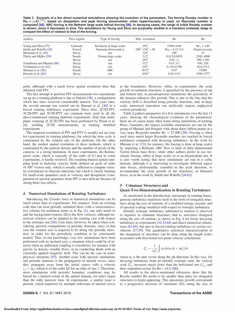
Table 2 Excerpts of a few direct numerical simulations showing the evolution of the parameters. The forcing Rossby number isRof 5 ðef k

2f Þ

1=3Þ, based on dissipation and peak forcing wavenumber; when hyperviscosity is used, no Reynolds number iscomputed [24]. ABC forcing is the Beltrami large scale helical forcing [56]. In decaying cases, the range of initial Rossby numberis shown, since it decreases in time. The simulations by Yeung and Zhou are purposely studied in a transient unsteady stage tocompare the effect of rotation to that of the forcing.

Authors Flow regime Type of forcing Max. resolution Ro Re

Yeung and Zhou [57] Unsteady Stochastic at large scales 2563 0.004–0.06 Rek ’ 140Smith and Waleffe [24] Forced Gaussian about peak kf 2003, 2562� 40 Rof¼ 0.12, 0.3 HyperviscosityMorinishi et al. [58] Decay n/a 1283 200 53Thiele and M€uller [59] Steady Frozen large scales 5123 0.013,0.0053 2300, 4000

Decay n/a 2563 0.02,1 300–1100Teitelbaum and Mininni [60] Decay n/a 5123 0.07, 0.1 450, 530Yoshimatsu et al. [61] Decay n/a 2563 0.119–0.596 56.6–93.2Mininni et al. [56] Steady ABC 30723 0.07 27000Delache et al. [62] Decay n/a 10243 0.02–0.51 1590–4777

030802-6 / Vol. 67, MAY 2015 Transactions of the ASME

Downloaded From: http://appliedmechanicsreviews.asmedigitalcollection.asme.org/ on 01/16/2015 Terms of Use: http://asme.org/terms

rotation [33]. The transition appearing at Ro�O(1) correspondsto a progressive extension of the range of scales at which the lin-ear effect of rotation dominates over nonlinear diffusion. Thisbegins in the large scales and extends progressively to smallerscales, in the case of decaying turbulence. When all scales beginto be affected by rotation, that is when the microscale Rossbynumber Rox ¼ x0=ð2XÞ � Oð1Þ, where x0 is the rms vorticity,the complete transition of the turbulent field to a quasi-two-dimensional state begins [66,67]. However, when considering thelimit Re ! 1 and Ro ! 0, the exactly two-dimensional state isnot achieved at finite times in infinite or periodic domains, sincethe energy keeps accumulating in a neighborhood kk ’ 0, but witha zero transfer rate at kk¼ 0. [10].

The two-dimensional manifold kk¼ 0 is, therefore, assumed toplay a particular role in the dynamics of rotating turbulence.Exactly two-dimensional flows are flows in which energy is onlycontained in the manifold characterized by a Dirac function d(kk)in wavenumber space, thus behaving with a two-dimensionaldynamics [68]. In rotating turbulence, the two-dimensional mani-fold is included in three-dimensional space, so that both two-dimensional and three-dimensional modes are coupled, althoughthe precise nature of this coupling is still investigated at the levelof inertial wave–vortex interactions. The corresponding energytransfers were investigated by forced numerical simulations bySmith and Waleffe [24] and in decaying turbulence simulationsby Bourouiba and Bartello [25]. In the former simulations, energyis transferred to the large scales from the smaller forced ones, thusfeeding the two-dimensional dynamics. In the decaying simula-tions, a maximum of energy transfer is observed, when varyingthe Rossby number, in the intermediate Ro regime for Ro ’ 0.2,and is the result of interactions between inertial waves and vorti-cal structures. In statistical models of inertial wave-turbulence, asa limit of rotating turbulence when Ro ! 0, an explicit couplingwith two-dimensional modes would have to be explicitly intro-duced to reproduce the transfer of energy toward the slow-manifold, and thus reproduce the wave–vortex interactions [69].

Although the anisotropization of rotating turbulence appearsrather clearly from the observation of structures elongated alongthe rotation axis, its detailed statistical characterization requires to

consider the dimensionality and the componentality of the flow,quantified by dedicated statistics. In short, in the case of rotatingflows, dimensionality reflects the accumulation of energy intoquasi-two-dimensional motion, and componentality is needed tosort the kind of structures that receive this energy: jetlike or vor-texlike. Similar refined statistics were introduced for flows withgeneral distortions other than rotation [70]. Componentalityappears upon computing the Reynolds stress tensor anisotropy

bij ¼dij

3� huiujihukuki

(3)

which is important for assessing the preferential directions inwhich the energy of the flow accumulates. This quantity is easilyaccessible in experiments. bii¼ 0 in incompressible flows, and,for isotropic turbulence, bij¼ 0. For axisymmetric turbulence,b11¼ b22, so that b33¼�2b11. b33 is also a relevant anisotropycomponent, since it not only reflects the axial fluid motion butalso contains an important information related to the way energyaccumulates in the neighborhood of the two-dimensionalmanifold.

The important difference between dimensionality and compo-nentality may be understood from the helical wave decompositionof the velocity field. Helical modes are the two eigenmodes N(k)of the curl operator, given a wavevector k, and were introducedfirst in the context of isotropic turbulence by Craya [71], then inaxisymmetric and stratified flows by Herring [72], and later usedin order to analyze the effect of the Coriolis term on turbulence[66,73]. For the sake of brevity, we shall refer to, e.g., Sagaut andCambon [5] for details, but in short, based on the helical modedecomposition, one is able to define three contributions to thetwo-point velocity correlation spectrum: (1) a part that containsthe energetic dependence on the wavevector orientation, e(k); (2)a polarization spectrum Z(k) that permits to assess the preemi-nence of one helical mode component of velocity over the other,so that when kk¼ 0, one is able to differentiate the axial contribu-tion—vertical energy—from the horizontal contribution to hori-zontal kinetic energy spectrum; (3) the helicity spectrum h(k).

Fig. 4 Organization of turbulence in columnar structures: (a) visualization by pearlescencetechnique in an experiment by Staplehurst (see Table 1), as reported by Dalziel (false colorsare applied to enhance the features of the flow). Turbulence decays behind a stroke of verti-cally towed grid, from left to right after 0.5, 1, 2, 4 inertial times X/2p after the grid left bottomof view. (Reproduced with permission from Dalziel [64]. Copyright 2011 by Cambridge Univer-sity). (b) Isosurface of intense vorticity regions in a subregion of a 2563 Direct Numerical Simu-lation by Yoshimatsu et al., from left to right at initial time then at Xt 5 5 at which Rox ’ 1, andat Xt 5 10 and 20. (Reproduced with permission from Yoshimatsu [61]. Copyright 2011 byCambridge University).

Applied Mechanics Reviews MAY 2015, Vol. 67 / 030802-7

Downloaded From: http://appliedmechanicsreviews.asmedigitalcollection.asme.org/ on 01/16/2015 Terms of Use: http://asme.org/terms

The latter is assumed here to be negligible, although this may notbe true in some simulations with specific helical forcing, as theABC one [56]. The value of the e, Z decomposition lies in theassociated dynamical equations

ð@t þ 2�k2ÞeðkÞ ¼ TeðkÞ (4)

ð@t þ 2�k2 � i4X cos hÞZðkÞ ¼ TzðkÞ (5)

where i2¼�1, and in which the right-hand-side terms are nonlin-ear transfer terms. Equation (5) shows that the evolution of Z(k)for horizontal modes, such that h¼ p/2, is only driven by nonlin-ear terms, and no direct linear effect of rotation applies. There-fore, if all the energy of the flow were to be accumulated in thetwo-dimensional manifold, rotation would have no effect on itsdynamics. This is consistent with the common knowledge thattwo-dimensional flows are not affected by rotation.

Turning back to the anisotropy tensor (3), it is possible todecompose b33 as be

33 þ bZ33, where each contribution originates

from e(k) and Z(k). In this decomposition, the anisotropy compo-nent b33 contains a part which is only driven by nonlinear dynam-ics (Eq. (4)) and a part that may still be affected by lineardynamics (Eq. (5)). The introduction of this decomposition is jus-tified when one computes the evolution of the two contributions indirect numerical simulations as shown on Fig. 5.

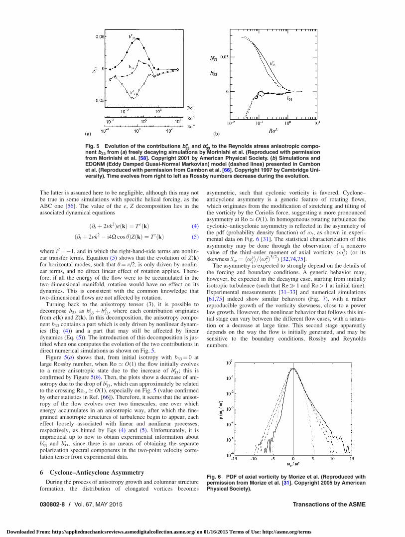
Figure 5(a) shows that, from initial isotropy with b33¼ 0 atlarge Rossby number, when Ro ’ O(1) the flow initially evolvesto a more anisotropic state due to the increase of be

33; this isconfirmed by Figure 5(b). Then, the plots show a decrease of ani-sotropy due to the drop of bz

33, which can approximately be relatedto the crossing Rox ’ O(1), especially on Fig. 5 (value confirmedby other statistics in Ref. [66]). Therefore, it seems that the anisot-ropy of the flow evolves over two timescales, one over whichenergy accumulates in an anisotropic way, after which the fine-grained anisotropic structures of turbulence begin to appear, eacheffect loosely associated with linear and nonlinear processes,respectively, as hinted by Eqs (4) and (5). Unfortunately, it isimpractical up to now to obtain experimental information aboutbe

33 and bz33, since there is no means of obtaining the separate

polarization spectral components in the two-point velocity corre-lation tensor from experimental data.

6 Cyclone–Anticyclone Asymmetry

During the process of anisotropy growth and columnar structureformation, the distribution of elongated vortices becomes

asymmetric, such that cyclonic vorticity is favored. Cyclone–anticyclone asymmetry is a generic feature of rotating flows,which originates from the modification of stretching and tilting ofthe vorticity by the Coriolis force, suggesting a more pronouncedasymmetry at Ro ’ O(1). In homogeneous rotating turbulence thecyclonic–anticyclonic asymmetry is reflected in the asymmetry ofthe pdf (probability density function) of xz, as shown in experi-mental data on Fig. 6 [31]. The statistical characterization of thisasymmetry may be done through the observation of a nonzerovalue of the third-order moment of axial vorticity hx3

z i (or itsskewness Sx ¼ hx3

z i=hx2z i

3=2) [32,74,75].

The asymmetry is expected to strongly depend on the details ofthe forcing and boundary conditions. A generic behavior may,however, be expected in the decaying case, starting from initiallyisotropic turbulence (such that Re� 1 and Ro> 1 at initial time).Experimental measurements [31–33] and numerical simulations[61,75] indeed show similar behaviors (Fig. 7), with a ratherreproducible growth of the vorticity skewness, close to a powerlaw growth. However, the nonlinear behavior that follows this ini-tial stage can vary between the different flow cases, with a satura-tion or a decrease at large time. This second stage apparentlydepends on the way the flow is initially generated, and may besensitive to the boundary conditions, Rossby and Reynoldsnumbers.

Fig. 5 Evolution of the contributions be33 and bz

33 to the Reynolds stress anisotropic compo-nent b33 from (a) freely decaying simulations by Morinishi et al. (Reproduced with permissionfrom Morinishi et al. [58]. Copyright 2001 by American Physical Society. (b) Simulations andEDQNM (Eddy Damped Quasi-Normal Markovian) model (dashed lines) presented in Cambonet al. (Reproduced with permission from Cambon et al. [66]. Copyright 1997 by Cambridge Uni-versity). Time evolves from right to left as Rossby numbers decrease during the evolution.

Fig. 6 PDF of axial vorticity by Morize et al. (Reproduced withpermission from Morize et al. [31]. Copyright 2005 by AmericanPhysical Society).

030802-8 / Vol. 67, MAY 2015 Transactions of the ASME

Downloaded From: http://appliedmechanicsreviews.asmedigitalcollection.asme.org/ on 01/16/2015 Terms of Use: http://asme.org/terms

One explanation for the asymmetry growth is provided by theanalytical derivation of Gence and Frick [76], which expresses thegrowth of hx3

z i at short time in a suddenly rotated isotropicturbulence

dhx3z i

dtðt ¼ 0þÞ ¼ 4

5Xhxixjsijiðt ¼ 0Þ

where sij is the rate of strain tensor. This predicts a linear growthof hx3

z i at short time, in qualitative agreement with the observa-tions, but the long-time behavior cannot be inferred from thisequation when sij becomes in turn modified by rotation. It isimportant to note that this process of emergence of dominantcyclonic motion from an initially isotropic state is different fromthe selection of cyclonic structures among pre-existing cyclonicand anti–cyclonic vortices [77]. The latter mechanism involvesthe stability of coherent structures, from various possible mecha-nisms, such centrifugal or elliptical instability.

An important open question is the scale dependence of theasymmetry: at what scales are the vortical structures that contrib-ute to the asymmetry? Does the asymmetry first appear at smallscales, or is it dominated by a few large-scale cyclones? Thiscould be probed from filtered vorticity field [33] or two-pointthird-order velocity correlation [48,63]. The answer probablydepends on whether the scales are larger or smaller than theZeman scale (the scale at which the turbulent time is of order ofthe global rotation, see below), although no systematic study hasbeen performed so far.

7 Spectral Scalings and Scale-by-Scale Anisotropy

From the observation of the anisotropic structure of rotatingturbulence, one expects that energy spectra E(k) exhibit scalingswhich differ from the Kolmogorov scaling k�5/3 of isotropic tur-bulence. Moreover, one may consider not only spherical spectra

that depend on the wavenumber k but also spectra that exhibit adirectional dependence, in the form e(k?, kk) where k? is thewavenumber component orthogonal to X, or in a similar guise e(k,h), separating scale k dependence from direction dependence. Inthe latter case, one considers the important horizontal spectrum ath¼ p/2, which is related to the quasi-two-dimensional dynamics,which can be obtained in the former case by setting kk¼ 0.

Theoretical, experimental, and numerical results about thescaling of the kinetic energy spectrum are available. In a phenom-enological study, Mahalov and Zhou [78,79] examine the differentcharacteristic timescales appearing in the long-term behavior ofrapidly rotating turbulence. They propose the following scaling(the Zhou spectrum): EðkÞ ¼ CXðXeÞ1=2k�2 considering only therotation timescale, for small k such that Ro< 1, which is correctedin EðkÞ ¼ C2ðkXÞ e2=3k�5=3 when both rotation and eddy-turnovertimescales are combined, for larger k at Ro> 1 (e is the kineticenergy dissipation). In the latter estimate, the prefactor isexpressed in terms of the Zeman wavenumber kX¼ (X3/e)1/2 thatappears to be an important scale as discussed further below. Whenconsidering turbulence forced at an intermediate wavenumber kf,as in simulations by Smith and Waleffe [24], different scalings arefound above and below the forcing wavenumber: for k< kf,E(k)� k�3 as in two-dimensional turbulence, which could be atrace of an inverse cascade; for k> kf, k�5/3 is recovered as befitsa forward Kolmogorov-like cascade down to the smallest scales.In the work by Mininni and Pouquet [13] in which turbulence isforced by a helical ABC flow at large scales, the energy spectrumscaling is k�5/3, but another cascade intervenes for the helicityspectrum that scales as k�2.

The fact that the small scales of rotating turbulence are stronglyanisotropic can be interpreted with the help of the Zeman wave-number kX¼ (X3/e)1/2, or the related Zeman length scale 2p/kX.Although defined a long time ago, this scale and its importancehas been supported by recent investigations into the anisotropy atthe various scales of rotating turbulence. These investigations

Fig. 7 Growth of axial vorticity skewness hx3z i=hx2

z i3=2 in experiments (top figures) and

numerical simulations (bottom figures): (a) Experimental data by Staplehurst et al. filled andopen symbols, respectively, at initial Ro ’ 0.37 and 0.41, two different rotation rates used.(Reproduced with permission from Staplehurst et al. [32]. Copyright 2008 by Cambridge Uni-versity.) (b) Experimental data by Morize et al. at Rog from 2.4 to 120. (Reproduced with permis-sion from Morize et al. [31]. Copyright 2005 by American Physical Society). (c) DNS (directnumerical simulation) data by Yoshimatsu et al. with Ro from 4.8 3 1022 to 0.24. (Reproducedwith permission from Yoshimatsu et al. [61]. Copyright 2011 by Cambridge University). (d)DNS data by van Bokhoven et al. at Rok from 0.073 to 0.37. (Reproduced with permission fromvan Bokhoven et al. [75]. Copyright 2008 by Taylor & Francis).

Applied Mechanics Reviews MAY 2015, Vol. 67 / 030802-9

Downloaded From: http://appliedmechanicsreviews.asmedigitalcollection.asme.org/ on 01/16/2015 Terms of Use: http://asme.org/terms

seem to demonstrate, both in experimental results [34] and innumerical simulations [56,62], that each turbulent scale can becompared to the Zeman scale to determine whether anisotropy ispresent or not, and that maximum anisotropy is found at scales oforder of the Zeman scale. For instance, in the simulations pre-sented in Fig. 8(a), but also in the simulations by Delache et al.[62], if kX> k for all wavenumbers k in the inertial range, rotationaffects all scales and renders them anisotropic. If kX is in an inter-mediate range, anisotropy affects the large scales only while iso-tropy is recovered for small scales. Therefore, it is necessary thatX be large enough with respect to the dissipation � for anisotropyto begin to appear, or, conversely, that the dissipation becomesmall enough—for instance in decaying turbulence—at fixed rota-tion rate.

The next refined description accounts for the directionaldependence of the spectra in the (k?, kk) spectral space, sincerotating turbulence is statistically axisymmetric. The theoreticalprediction by Galtier [80] in a wave turbulence framework, agree-ing with rapidly rotating turbulence, is based on the helical modesdecomposition, and provides the anisotropic energy spectrumscaling Eðk?; kkÞ � k

�5=2? k

�1=2

k —the k? power may vary if onetakes into account a low-wavenumber spectral cut-off inthe k? direction [81]—and Hðk?; kkÞ � k

�3=2? k

�1=2

k for the helicityspectrum. In the asymptotic low Rossby number limit, the theoret-ical scalings of helicity and energy spectra are shown to be linked[82]. The theory also confirms that, to lowest order, the two-dimensional modes are not dynamically coupled to the three-dimensional wave-turbulence. The simulations by Mininni et al.[56] seem to confirm the k�5/2 scaling of the spectrum, but onlyfor the kk¼ 0 contribution, and for scales larger than the Zemanscale. For smaller scales, the k�5/3 scaling is again recovered. Innonhelically large-scale forced simulations by Thiele and M€uller[59], the horizontal spectral scaling for energy is found to beEðk?; kk ¼ 0Þ � k�2

? , but the authors show that the scaling of thefull spectrum is Eðk?Þ � k�3

? close to the two-dimensional mani-fold, and is the result of integration over kk, hence underliningthe important difference between one-dimensional spectra andintegrated spectra.

An example of directional spectral dependence with respect tok, h, which contains the same information as the k?, kk depend-ence, is shown in Fig. 8. It shows that the largest anisotropy, interms of horizontal-to-vertical energy difference at a given k,appears in the smallest scales, both in simulations (Fig. 8(a) [61])and in a two-point statistical model (Fig. 8(b) [69]) for weakinertial wave turbulence. In the latter, the horizontal mode is not

represented, so that the vertical separation of the most energeticspectrum appearing in Fig. 8(b) already hints at a decoupling ofthe neighborhood of the slow manifold.

8 Balance Statistical Equations in Physical and

Spectral Formalisms and Related Dynamics

The interpretation of the above results requires a careful exami-nation of the dynamical equations. We thus consider the balanceequations for two-point statistics, obtained from Eq. (1). It permitsto examine the dynamics of the flow in terms of scales, and toobtain a diagnostic of the scale-by-scale exchanges. Consideringthe trace of the two-point velocity correlation tensor R ¼ RiiðrÞ¼ huiðxÞuiðxþ rÞi, one derives the Karman–Howarth–Moninequation

1

2@tR ¼

1

4r � Fþ �r2R (6)

in which the flux term F ¼ hduðdu � duÞi is a third-order quantitybased on the velocity increments du ¼ uðxþ rÞ � uðxÞ (see, e.g.,Ref. [83]). In isotropic turbulence F is aligned with the separationvector r and, for scales jrj in the inertial range, Eq. (6) integratesto the famous 4/5th law, Fr¼�(4/5)er, with e¼�dtR(r¼ 0)/2 theenergy dissipation rate. The central question here is to model thisanisotropic flux F in the presence of rotation.

No explicit effect of rotation appears in Eq. (6), since the Corio-lis force, being orthogonal to u by nature, does no work, but rota-tion appears in the dynamical equation for F. It therefore requiredphenomenological scaling arguments to Galtier [84] to be able topropose a functional dependence of the flux term with respect tothe direction of the separation vector, in rotating turbulence.

The analogous of the Karman–Howarth–Monin equation inspectral space is the Lin equation, which has a similar structure,wherein the third-order terms in the right-hand-side are exactlythe nonlinear energy transfer for a given wavenumber k ofenergy E(k)

@tEðkÞ ¼ TðkÞ � 2�k2EðkÞ (7)

Note that the Lin equation is an integrated version of the energydensity equation similar to Eq. (4), the integration over the anglesbeing used to remove the explicit h dependence. Note also that theother spectral equation (5) for the polarization spectrum is notreflected in Eq. (6) in terms of physical contents.

Fig. 8 Directional spectra E(k,h) from (a) direction numerical simulations by Yoshimatsu et al.(Reproduced with permission from Yoshimatsu et al. [61]. Copyright 2011 by Cambridge Uni-versity). (b) From the two-point statistical AQNM (asymptotic quasi-normal Markovian) modelby Bellet et al. (Reproduced with permission from Bellet et al. [69]. Copyright 2006 by Cam-bridge University). The lower spectra are for the vertical direction h’p/2, the upper ones forthe horizontal spectra at h’0. In the simulations, four angular sectors of h are used to com-pute the statistical averages, whereas in the AQNM model, spectra correspond to discreteorientations.

030802-10 / Vol. 67, MAY 2015 Transactions of the ASME

Downloaded From: http://appliedmechanicsreviews.asmedigitalcollection.asme.org/ on 01/16/2015 Terms of Use: http://asme.org/terms

As mentioned in Sec. 3, the computation of the different termsin Eq. (6) has been rendered possible from experimental resultswhen PIV techniques began to be developed. Interestingly, fromdirect numerical simulations, Eq. (7) only was used, since, fromspectral simulation methods, one has a rather easy access to theenergy transfer term T(k). But this term bears the same informa-tion as ð1=4Þr � F in Eq. (6).

Obtaining experimental evaluations of the different terms inEq. (6) requires a significant experimental effort, since third-ordermoments are prone to statistical noise. In a first dedicated settingusing only two-dimensional measurements that permit to obtain

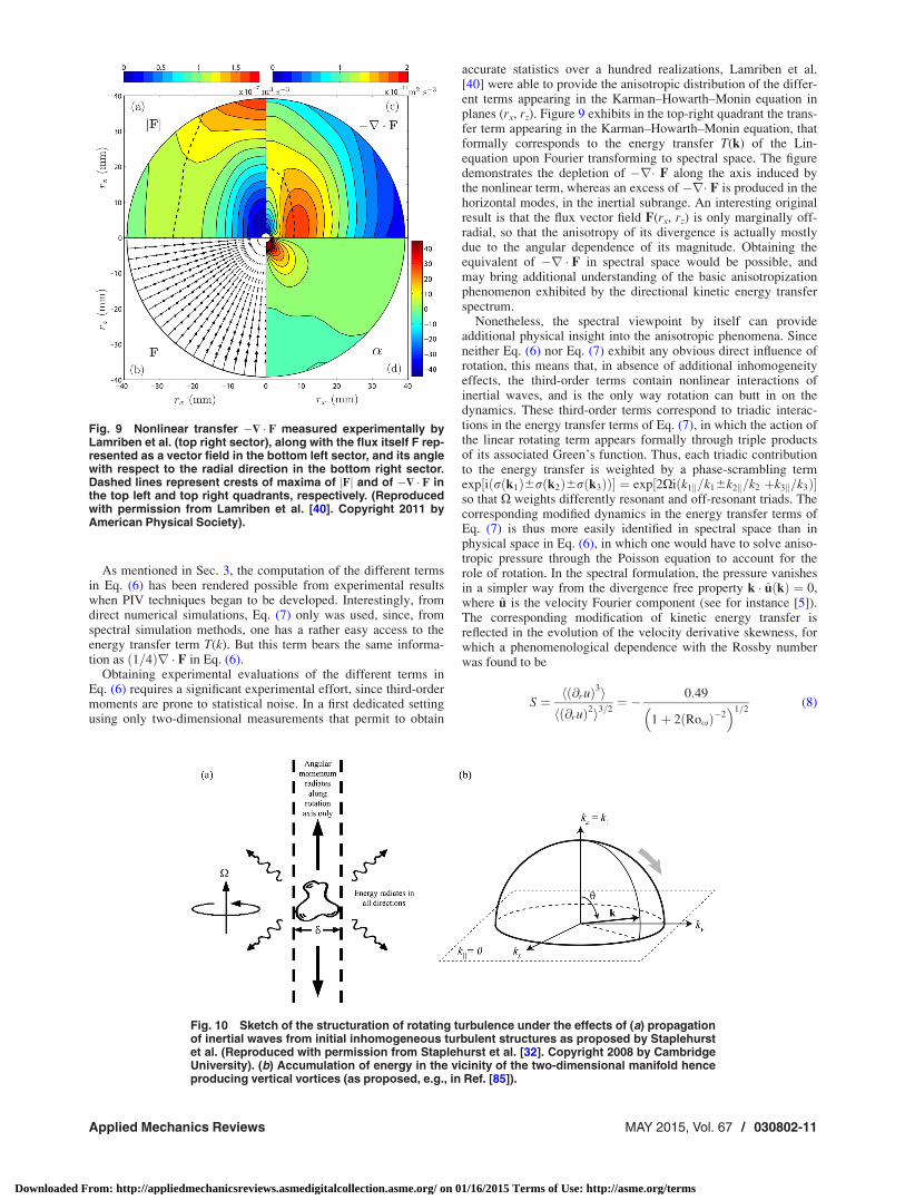
accurate statistics over a hundred realizations, Lamriben et al.[40] were able to provide the anisotropic distribution of the differ-ent terms appearing in the Karman–Howarth–Monin equation inplanes (rx, rz). Figure 9 exhibits in the top-right quadrant the trans-fer term appearing in the Karman–Howarth–Monin equation, thatformally corresponds to the energy transfer T(k) of the Lin-equation upon Fourier transforming to spectral space. The figuredemonstrates the depletion of �r� F along the axis induced bythe nonlinear term, whereas an excess of �r� F is produced in thehorizontal modes, in the inertial subrange. An interesting originalresult is that the flux vector field F(rx, rz) is only marginally off-radial, so that the anisotropy of its divergence is actually mostlydue to the angular dependence of its magnitude. Obtaining theequivalent of �r � F in spectral space would be possible, andmay bring additional understanding of the basic anisotropizationphenomenon exhibited by the directional kinetic energy transferspectrum.

Nonetheless, the spectral viewpoint by itself can provideadditional physical insight into the anisotropic phenomena. Sinceneither Eq. (6) nor Eq. (7) exhibit any obvious direct influence ofrotation, this means that, in absence of additional inhomogeneityeffects, the third-order terms contain nonlinear interactions ofinertial waves, and is the only way rotation can butt in on thedynamics. These third-order terms correspond to triadic interac-tions in the energy transfer terms of Eq. (7), in which the action ofthe linear rotating term appears formally through triple productsof its associated Green’s function. Thus, each triadic contributionto the energy transfer is weighted by a phase-scrambling termexp½iðrðk1Þ6rðk2Þ6rðk3ÞÞ� ¼ exp½2Xiðk1k=k16k2k=k2 þk3k=k3Þ�so that X weights differently resonant and off-resonant triads. Thecorresponding modified dynamics in the energy transfer terms ofEq. (7) is thus more easily identified in spectral space than inphysical space in Eq. (6), in which one would have to solve aniso-tropic pressure through the Poisson equation to account for therole of rotation. In the spectral formulation, the pressure vanishesin a simpler way from the divergence free property k � uðkÞ ¼ 0,where u is the velocity Fourier component (see for instance [5]).The corresponding modification of kinetic energy transfer isreflected in the evolution of the velocity derivative skewness, forwhich a phenomenological dependence with the Rossby numberwas found to be

S ¼ hð@ruÞ3ihð@ruÞ2i3=2

¼ � 0:49

1þ 2 Roxð Þ�2� �1=2

(8)

Fig. 9 Nonlinear transfer �$ � F measured experimentally byLamriben et al. (top right sector), along with the flux itself F rep-resented as a vector field in the bottom left sector, and its anglewith respect to the radial direction in the bottom right sector.Dashed lines represent crests of maxima of jFj and of �$ � F inthe top left and top right quadrants, respectively. (Reproducedwith permission from Lamriben et al. [40]. Copyright 2011 byAmerican Physical Society).

Fig. 10 Sketch of the structuration of rotating turbulence under the effects of (a) propagationof inertial waves from initial inhomogeneous turbulent structures as proposed by Staplehurstet al. (Reproduced with permission from Staplehurst et al. [32]. Copyright 2008 by CambridgeUniversity). (b) Accumulation of energy in the vicinity of the two-dimensional manifold henceproducing vertical vortices (as proposed, e.g., in Ref. [85]).

Applied Mechanics Reviews MAY 2015, Vol. 67 / 030802-11

Downloaded From: http://appliedmechanicsreviews.asmedigitalcollection.asme.org/ on 01/16/2015 Terms of Use: http://asme.org/terms

This dependence shows that, from the classical isotropic value�0.49 at large Rossby number when rotation is weak, the skew-ness steadily decreases upon increasing the rotation rate. Thefunctional dependence (8) proposed by Cambon et al. [66] fromresults of direct numerical simulations and of two-point statisticalmodeling of rotating turbulence is also well verified by experi-mental data [31].

It is also interesting to discuss the interpretation of the mecha-nism of creation of elongated structures and of anisotropy in rotat-ing turbulence, with two points of view. On the one hand, theabove mechanism explains the structuration by nonlinear phenom-ena transferring energy toward the two-dimensional manifold (seeFig. 10(b)); on the other hand, the interpretation proposed byStaplehurst et al. [32] based on the linear propagation of inertialwaves along the rotation axis from initial turbulent patches (seeFig. 10(a)). In order to reconcile both approaches, one could pro-pose a combination of the two mechanisms, wherein, on the onehand, turbulent blobs—originating from initial conditions or tur-bulence forcing mechanisms—are propagated vertically over asmall timescale based on Ro�1, and, on the other hand, nonlinearinteractions set in over a longer timescale based on Ro�2. Depend-ing on the specific parameter of each flow, and considering thefact that most experiments and direct numerical simulations arestill in a moderate Rossby number range Ro¼O(1), these twophenomena may be mingled, and can overlap for some time. Thiscould explain the various observations and differing behaviors inexperimental or numerical statistics of rotating turbulence.

9 Conclusions

This review contains a snapshot of selected recent results andmechanisms in the study of rotating turbulence. In terms of thestructural characterization of the flow, modern metrology used inexperiments permit to obtain a refined picture of not only thevelocity field topology but also the axisymmetric velocity fieldstatistics, including high-order moments. The current resolution ofPIV and PTV is still not able to provide the complete small-scaledynamics, especially for a good estimate of the dissipative scales,but progress is expected in the near future. Computer power isalso rapidly increasing, and the larger resolution direct numericalsimulations of rotating turbulence currently provide a good sepa-ration of scales necessary to understand its complex dynamics.There is still some way though before one will be able to computea flow for instance combining rotation and stable stratificationeffects in proportion of those observed in the atmosphericboundary layer, since the required scale separation and Reynoldsnumber value are currently beyond our reach, computationallyspeaking. In addition to these efforts, modeling can still beimproved, especially regarding the coupling between the two-dimensional turbulent manifold and the three-dimensional wavefield. A self-consistent theory for rotating turbulence, and, start-ing, for more general axisymmetric turbulence, in the guise ofKolmogorov’s for isotropic turbulence, is yet to be developed.

Acknowledgment

F.M. would like to thank the Institut Universitaire de Francefor its support, and the Agence Nationale de la Recherche throughGrant No. ANR- 2011-BS04-006-01. F.S.G. acknowledges thesupport of Agence Nationale de la Recherche through Grant No.ANR-08-BLAN-0076.

References[1] Barnes, S. A., 2001, “An Assessment of the Rotation Rates of the Host Stars of

Extrasolar Planets,” Astrophys. J., 561(2), pp. 1095–1106.[2] Cho, J. Y.-K., Menou, K., Hansen, B. M. S., and Seager, S., 2008,

“Atmospheric Circulation of Close-in Extrasolar Giant Planets: I. Global, Baro-tropic, Adiabatic Simulations,” Astrophys. J., 675(1), pp. 817–845.

[3] Dumitrescu, H., and Cardos, V., 2004. “Rotational Effects on the Boundary-Layer Flow in Wind Turbines,” AIAA J., 42(2), pp. 408–411.

[4] Praud, O., Sommeria, J., and Fincham, A., 2006, “Decaying Grid Turbulence ina Rotating Stratified Fluid,” J. Fluid Mech., 547, p. 389.

[5] Sagaut, P., and Cambon, C., 2008, Homogeneous Turbulence Dynamics,Cambridge University, Cambridge, UK.

[6] Greenspan, H. P., 1968, The Theory of Rotating Fluids, Cambridge University,Cambridge, UK.

[7] Bennetts, D. A., and Hocking, L. M., 1973, “On Nonlinear Ekman and Stewart-son Layers in a Rotating Fluid,” Proc. R. Soc. London, Ser. A, 333(1595), pp.469–489.

[8] Taylor, G. I., 1917, “Motion of Solids in Fluids When The Flow Is NotIrrotational,” Proc. R. Soc. London, Ser. A, 93(648), pp. 99–113.

[9] Proudman, J., 1916, “On the Motion of Solids in a Liquid Possessing Vorticity,”Proc. R. Soc. London, Ser. A, 92(642), pp. 408–424.

[10] Babin, A., Mahalov, A., and Nicolaenko, B., 2000, “Global Regularity of 3DRotating Navier-Stokes Equations for Resonant Domains,” Appl. Math. Lett.,13(4), pp. 51–57.

[11] Zeman, O., 1994, “A Note on the Spectra and Decay of Rotating HomogeneousTurbulence,” Phys. Fluids, 6(10), p. 3221.

[12] Batchelor, G. K., 2000, An Introduction to Fluid Dynamics, Cambridge Univer-sity, Cambridge, UK.

[13] Mininni, P. D., and Pouquet, A., 2010, “Rotating Helical Turbulence. I. GlobalEvolution and Spectral Behavior,” Phys. Fluids, 22(3), p. 035105.

[14] Lamriben, C., Cortet, P.-P., and Moisy, F., 2011, “Direct Measurements of Ani-sotropic Energy Transfers in a Rotating Turbulence Experiment,” Phys. Rev.Lett., 107, p. 024503.

[15] Davidson, P. A., 2013, Turbulence in Rotating, Stratified and Electrically Con-ducting Fluids, Cambridge University, New York.

[16] Lighthill, M., 1978, Waves in Fluids, Cambridge University, New York.[17] G€ortler, H., 1957, “On Forced Oscillations in Rotating Fluids,” Proceedings of

the Fifth Midwestern Conference on Fluid Mechanics, The University of Michi-gan, Ann Arbor, MI, Apr. 1–2, pp. 1–10.

[18] Cortet, P.-P., Lamriben, C., and Moisy, F., 2010, “Viscous Spreading of anInertial Wave Beam in a Rotating Fluid,” Phys. Fluids, 22(8), p. 086603.

[19] Maas, L. R. M., 2001, “Wave Focusing and Ensuing Mean Flow due to Symme-try Breaking in Rotating Fluids,” J. Fluid Mech., 437, pp. 13–28.

[20] Nazarenko, S., 2011, Wave Turbulence, Springer, Berlin.[21] Smith, L. M., and Lee, Y., 2005, “On Near Resonances and Symmetry Breaking

in Forced Rotating Flows at Moderate Rossby Number,” J. Fluid Mech., 535,p. 111.

[22] Bourouiba, L., Straube, D. N., and Waite, M. L., 2012, “Non-Local EnergyTransfers in Rotating Turbulence at Intermediate Rossby Number,” J. FluidMech., 690, pp. 129–147.

[23] Bourouiba, L., 2008, “Discreteness and Resolution Effects in Rapidly RotatingTurbulence,” Phys. Rev. E, 78, p. 056309.

[24] Smith, L., and Waleffe, F., 1999, “Transfer of Energy to Two-DimensionalLarge Scales in Forced, Rotating Three-Dimensional Turbulence,” Phys. Fluids,11(6), pp. 1608–1622.

[25] Bourouiba, L., and Bartello, P., 2007, “The Intermediate Rossby Number Rangeand Two-Dimensional–Three-Dimensional Transfers in Rotating DecayingHomogeneous Turbulence,” J. Fluid Mech., 587, pp. 139–161.

[26] Scott, J., 2014, “Wave Turbulence in a Rotating Channel,” J. Fluid Mech., 741,pp. 316–349.

[27] Wigeland, R. A., and Nagib, H. M., 1978, “Grid-Generated Turbulence Withand Without Rotation About the Streamwise Direction,” IIT Fluid and HeatTransfer Report No. R78-1, Illinois Institute of Technology, Chicago, IL.

[28] Jacquin, L., Leuchter, O., Cambon, C., and Mathieu, J., 1990, “HomogeneousTurbulence in the Presence of Rotation,” J. Fluid Mech., 220, pp. 1–52.

[29] Ibbetson, A., and Tritton, D. J., 1975, “Experiments on Turbulence in a Rotat-ing Fluid,” J. Fluid Mech., 68(4), pp. 639–672.

[30] Dalziel, S., 1992, “Decay of Rotating Turbulence: Some Particle TrackingExperiments,” Appl. Sci. Res., 49(3), pp. 217–244.

[31] Morize, C., Moisy, F., and Rabaud, M., 2005, “Decaying Grid-GeneratedTurbulence in a Rotating Tank,” Phys. Fluids, 17(9), p. 095105.

[32] Staplehurst, P. J., Davidson, P. A., and Dalziel, S. B., 2008, “Structure Forma-tion in Homogeneous, Freely Decaying, Rotating Turbulence,” J. Fluid Mech.,598, pp. 81–103.

[33] Moisy, F., Morize, C., Rabaud, M., and Sommeria, J., 2011, “Decay Laws, Ani-sotropy and Cyclone-Anticyclone Anisotropy in Decaying RotatingTurbulence,” J. Fluid Mech., 666, pp. 5–35.

[34] Davidson, P. A., Staplehurst, P. J., and Dalziel, S. B., 2006, “On the Evolutionof Eddies in a Rapidly Rotating System,” J. Fluid Mech., 557, pp. 135–144.

[35] Hopfinger, E., Browand, P., and Gagne, Y., 1982, “Turbulence and Waves in aRotating Tank,” J. Fluid Mech., 125, p. 505.

[36] Dickinson, S. C., and Long, R. R., 1983, “Oscillating-Grid Turbulence Includ-ing Effects of Rotation,” J. Fluid Mech., 126, pp. 315–333.

[37] Bokhoven, L. J. A. V., Clercx, H. J. H., Heijst, G. J. F. V., and Trieling, R. R.,2009, “Experiments on Rapidly Rotating Turbulent Flows,” Phys. Fluids, 21(9),p. 096601.

[38] Baroud, C. N., Plapp, B. B., She, Z.-S., and Swinney, H. L., 2002, “AnomalousSelf-Similarity in a Turbulent Rapidly Rotating Fluid,” Phys. Rev. Lett., 88,p. 114501.

[39] Del Castello, L., and Clercx, H. J. H., 2011, “Lagrangian Velocity Auto-correlations in Statistically Steady Rotating Turbulence,” Phys. Rev. E, 83(5),p. 056316.

[40] Lamriben, C., Cortet, P.-P., and Moisy, F., 2011, “Direct Measurements of Ani-sotropic Energy Transfers in a Rotating Turbulence Experiment,” Phys. Rev.Lett., 107(2), p. 024503.

030802-12 / Vol. 67, MAY 2015 Transactions of the ASME

Downloaded From: http://appliedmechanicsreviews.asmedigitalcollection.asme.org/ on 01/16/2015 Terms of Use: http://asme.org/terms

[41] Kinzel, M., Holzner, M., L€uthi, B., Tropea, C., Kinzelbach, W., and Oberlack,M., 2009, “Experiments on the Spreading of Shear-Free Turbulence Under theInfluence of Confinement and Rotation,” Exp. Fluids, 47(4–5), pp. 801–809.

[42] Kinzel, M., Wolf, M., Holzner, M., L€uthi, B., Tropea, C., and Kinzelbach, W.,2010, “Simultaneous Two-Scale 3D-PTV Measurements in Turbulence Underthe Influence of System Rotation,” Exp. Fluids, 51(1), pp. 75–82.

[43] Ruppert-Felsot, J., Praud, O., Sharon, E., and Swinney, H., 2005, “Extraction ofCoherent Structures in a Rotating Turbulent Flow Experiment,” Phys. Rev. E,72(1), p. 016311.

[44] Kolvin, I., Cohen, K., Vardi, Y., and Sharon, E., 2009, “Energy Transfer byInertial Waves During the Buildup of Turbulence in a Rotating System,” Phys.Rev. Lett., 102(1), p. 014503.

[45] Yarom, E., Vardi, Y., and Sharon, E., 2013, “Experimental Quantification ofInverse Energy Cascade in Deep Rotating Turbulence,” Phys. Fluids, 25(8),p. 085105.

[46] Del Castello, L., and Clercx, H. J. H., 2011, “Lagrangian Acceleration of Pas-sive Tracers in Statistically Steady Rotating Turbulence,” Phys. Rev. Lett.,107(21), p. 214502.

[47] Del Castello, L., and Clercx, H. J., 2013, “Geometrical Statistics of the Vortic-ity Vector and the Strain Rate Tensor in Rotating Turbulence,” J. Turbul.,14(10), pp. 19–36.

[48] Gallet, B., Campagne, A., Cortet, P.-P., and Moisy, F., 2014, “Scale-DependentCyclone-Anticyclone Asymmetry in a Forced Rotating TurbulenceExperiment,” Phys. Fluids, 26(3), p. 035108.

[49] Simand, C., Chill�a, F., and Pinton, J.-F., 2000, “Inhomogeneous Turbulence inthe Vicinity of a Large-Scale Coherent Vortex,” Europhys. Lett. (EPL), 49(3),pp. 336–342.

[50] Lamriben, C., Cortet, P.-P., Moisy, F., and Maas, L. R. M., 2011, “Excitation ofInertial Modes in a Closed Grid Turbulence Experiment Under Rotation,” Phys.Fluids, 23(1), p. 015102.

[51] Ferrero, E., Mortarini, L., Manfrin, M., Longhetto, A., Genovese, R., and Forza,R., 2009, “Boundary-Layer Stress Instabilities in Neutral, Rotating TurbulentFlows,” Boundary Layer Meteorol., 130(3), pp. 347–363.

[52] Bewley, G. P., Lathrop, D. P., Maas, L. R. M., and Sreenivasan, K. R., 2007,“Inertial Waves in Rotating Grid Turbulence,” Phys. Fluids, 19(7), p. 071701.

[53] Ott, S., and Mann, J., 2000, “An Experimental Investigation of the Relative Dif-fusion of Particle Pairs in Three-Dimensional Turbulent Flow,” J. Fluid Mech.,422, pp. 207–223.

[54] Morinishi, Y., Nakabayashi, K., and Ren, S., 2001, “A New DNS Algorithm forRotating Homogeneous Decaying Turbulence,” Int. J. Heat Fluid Flow, 22(1),pp. 30–38.

[55] Brandenburg, A., Svedin, A., and Vasil, G. M., 2009, “Turbulent Diffusion WithRotation or Magnetic Fields,” Mon. Not. R. Astron. Soc., 395(3), pp. 1599–1606.

[56] Mininni, P., Rosenberg, D., and Pouquet, A., 2012, “Isotropisation at SmallScales of Rotating Helically Driven Turbulence,” J. Fluid Mech., 699,pp. 263–279.

[57] Yeung, P. K., and Zhou, Y., 1998, “Numerical Study of Rotating TurbulenceWith External Forcing,” Phys. Fluids, 10(11), pp. 2895–2909.

[58] Morinishi, Y., Nakabayashi, K., and Ren, S. Q., 2001, “Dynamics of Anisotropyon Decaying Homogeneous Turbulence Subjected to System Rotation,” Phys.Fluids, 13(10), pp. 2912–2922.

[59] Thiele, M., and M€uller, W.-C., 2009, “Structure and Decay of Rotating Homo-geneous Turbulence,” J. Fluid Mech., 637, pp. 425–442.

[60] Teitelbaum, T., and Mininni, P., 2010, “Large-Scale Effects on the Decay ofRotating Helical and Non-Helical Turbulence,” Phys. Scr., 2010, p. 014003.

[61] Yoshimatsu, K., Midorikawa, M., and Kaneda, Y., 2011, “Columnar Eddy For-mation in Freely Decaying Homogeneous Rotating Turbulence,” J. FluidMech., 677, pp. 154–178.

[62] Delache, A., Cambon, C., and Godeferd, F., 2014, “Scale by Scale Anisotropyin Freely Decaying Rotating Turbulence,” Phys. Fluids, 26(2), p. 025104.

[63] Deusebio, E., Boffetta, G., Lindborg, E., and Musacchio, S., 2014, “DimensionalTransition in Rotating Turbulence,” Phys. Rev. E, 90, p. 023005.

[64] Dalziel, S. B., 2011, “The Twists and Turns of Rotating Turbulence,” J. FluidMech., 666, pp. 1–4.

[65] Teitelbaum, T., and Mininni, P. D., 2011, “The Decay of Turbulence in Rotat-ing Flows,” Phys. Fluids, 23(6), p. 065105.

[66] Cambon, C., Mansour, N. N., and Godeferd, F. S., 1997, “Energy Transfer inRotating Turbulence,” J. Fluid Mech., 337, pp. 303–332.

[67] Canuto, V. M., and Dubovikov, M. S., 1997, “A Dynamical Model for Turbu-lence. v. the Effect of Rotation,” Phys. Fluids, 9(7), pp. 2132–2140.

[68] Kraichnan, R. H., 1975, “Statistical Dynamics of Two-Dimensional Flow,”J. Fluid Mech., 67(1), pp. 155–175.

[69] Bellet, F., Godeferd, F. S., Scott, J. F., and Cambon, C., 2006, “Wave Turbu-lence in Rapidly Rotating Flows,” J. Fluid Mech., 562, pp. 83–121.

[70] Kassinos, S. C., Reynolds, W. C., and Roger, M. M., 2001, “One-Point Turbu-lence Structure Tensors,” J. Fluids. Mech., 428, pp. 213–248.

[71] Craya, A., 1958, “Contribution �a l’analyse de la turbulence associ�ee �a des vit-esses moyennes,” Rev. Sci. et Tech. du Ministere de l’Air (France), 345.

[72] Herring, J. R., 1974, “Approach of Axisymmetric Turbulence to Isotropy,”Phys. Fluids, 17(5), pp. 859–872.

[73] Waleffe, F., 1993, “Inertial Transfers in the Helical Decomposition,” Phys. Flu-ids A, 5(3), p. 026310.

[74] Bartello, P., Metais, O., and Lesieur, M., 1994, “Coherent Structures in Rotat-ing 3-Dimensional Turbulence,” J. Fluid Mech., 273, pp. 1–29.

[75] van Bokhoven, L., Cambon, C., Liechtenstein, L., Godeferd, F., and Clercx, H.,2008, “Refined Vorticity Statistics of Decaying Rotating Three-DimensionalTurbulence,” J. Turbul., 9, N6.

[76] Gence, J. N., and Frick, C., 2001, “Birth of the Triple Correlations of Vorticityin an Homogeneous Turbulence Submitted to a Solid Body Rotation,” C. R.Acad. Sci. Paris, S�erie IIB, 329(4), pp. 351–356.

[77] Sreenivasan, B., and Davidson, P. A., 2008, “On the Formation ofCyclones and Anticyclones in a Rotating Fluid,” Phys. Fluids, 20(8),p. 085104.

[78] Zhou, Y., 1995, “A Phenomenological Treatment of Rotating Turbulence,”Phys. Fluids, 7(8), pp. 2092–2094.

[79] Mahalov, A., and Zhou, Y., 1996, “Analytical and Phenomenological Studiesof Rotating Turbulence,” Phys. Fluids, 8(8), pp. 2138–2152.

[80] Galtier, S., 2003, “Weak Inertial-Wave Turbulence Theory,” Phys. Rev. E, 68,p. 015301.

[81] Cambon, C., Rubinstein, R., and Godeferd, F. S., 2004, “Advances in Wave-Turbulence: Rapidly Rotating Flows,” New J. Phys., 6, 73.

[82] Galtier, S., 2014, “Theory for Helical Turbulence Under Fast Rotation,” Phys.Rev. E, 89, p. 041001.

[83] Frisch, U., 1995, Turbulence. The Legacy of A. N. Kolmogorov, CambridgeUniversity, Cambridge.

[84] Galtier, S., 2009, “Exact Vectorial Law for Homogeneous RotatingTurbulence,” Phys. Rev. E, 80(4), p. 046301.

[85] Godeferd, F., and Cambon, C., 1994, “Detailed Investigation of EnergyTransfers in Homogeneous Stratified Turbulence,” Phys. Fluids, 6(6), pp.2084–2100.

Applied Mechanics Reviews MAY 2015, Vol. 67 / 030802-13

Downloaded From: http://appliedmechanicsreviews.asmedigitalcollection.asme.org/ on 01/16/2015 Terms of Use: http://asme.org/terms