structural scenario analysis with svars
TRANSCRIPT

Structural Scenario Analysis with SVARs1
Juan Antolın-Dıaza, Ivan Petrellab, Juan F. Rubio-Ramırezc
aLondon Business SchoolbUniversity of Warwick
cEmory University, Federal Reserve Bank of Atlanta
Abstract
Macroeconomists seeking to construct conditional forecasts often face a choice between taking
a stand on the details of a fully-specified structural model or relying on empirical correlations
from vector autoregressions and remain silent about the underlying causal mechanisms. This
paper develops tools for constructing “structural scenarios” that can be given an economic
interpretation using identified structural VARs. We provide a unified and transparent
treatment of conditional forecasting and structural scenario analysis and relate our approach
to entropic forecast tilting. We advocate for a careful treatment of uncertainty, making the
methods suitable for density forecasting and risk assessment. We also propose a metric to
assess and compare the plausibility of alternative scenarios. We illustrate our methods with
two applications: assessing the power of forward guidance about future interest rate policies
and stress testing the reaction of bank profitability to an economic recession.
Keywords: Conditional forecasts, SVARs, Bayesian methods, forward guidance, stress
testing.
1. Introduction
Macroeconomists and policy analysts are routinely required to answer questions of the
form: “If, for the next few quarters, variable x were to follow alternative paths, how would
1We are grateful to Nabeel Abdoula, Piotr Chmielowski, Gavyn Davies, Domenico Giannone, JonasHallgren, Marek Jarocinski, Giulio Nicoletti, Giuseppe Ragusa, Paolo Surico, Fabrizio Venditti, and seminarparticipants at Warwick Business School, European Central Bank, Bank of England, London Business School,Bank of Spain, Banca d’Italia, and Central Bank of Ireland for helpful comments and suggestions. YadSelvakumar provided excellent research assistance. The views expressed here are those of the authors and donot necessarily reflect the views of the Federal Reserve Bank of Atlanta or the Federal Reserve System.

the forecasts of other variables change?” Uses of these conditional forecasts include assessing
the impact of alternative paths for policy instruments, incorporating external information
into model forecasts, and “stress testing” asset prices or bank profits against the onset of an
economic downturn. In practice, researchers often face a choice between taking a stand on
the details of a fully-fledged DSGE model (see Del Negro and Schorfheide, 2013) or relying
on reduced-form conditional forecasts from vector autoregression (VAR) models, as proposed
by Doan et al. (1986) and Waggoner and Zha (1999). A limitation of the latter approach is
that it relies on the empirical correlations among the variables in the system, and is therefore
silent about the underlying causal mechanisms behind the results. This can often severely
confound the interpretation of conditional forecasts.
This paper develops a unified and transparent treatment of both conditional forecasting
and structural scenario analysis with structural VAR (SVAR) models. We define a structural
scenario as a combination of a path for one or more variables in the system, and a restriction
that only a chosen subset of structural shocks can deviate from their unconditional distribution.
This exercise requires identifying economically meaningful shocks. We provide closed-form
solutions for the distribution of the variables and the underlying shocks under the restrictions.
In addition, we demonstrate the equivalence of our formulae to the entropic tilting method
popularized by Robertson et al. (2005). Another contribution, which follows naturally from
the connection to entropic tilting, is to propose a metric based on the Kullback-Leibler
divergence to assess the plausibility of a given scenario. Generalizing the “modest policy
interventions” of Leeper and Zha (2003), it quantifies the degree to which a scenario involves
a moderate deviation from the unconditional distribution of the shocks, in which case the
results of the analysis are likely to be reliable. In this way, we follow the tradition of Sims
(1986) in wanting to provide practical tools for macroeconomic analysis whenever one does
not want to commit to a particular DSGE model, while retaining a healthy dose of skepticism
about the limits of structural scenarios using linear models, as stressed by Lucas (1976).
Illustrative example. To highlight the importance of specifying the structural shocks driving
a particular scenario, consider an SVAR including output growth, inflation, and the fed funds
rate, which will be analyzed in detail in our empirical application. Figure 1 compares the
2

different answers that arise from the classic conditional forecasting question (“What is the
likely path of output and inflation, given that the fed funds rate is reduced to 1% and kept
there for two years?”) and an alternative one, which we call a structural scenario: “What is
the likely path of output and inflation, if monetary policy shocks lower the fed funds rate to
1% and keep it there for two years?”2 In the latter case, only the policy shocks are allowed
to deviate from their unconditional distribution to match the desired interest rate path. As
we can see, for the exact same path of the interest rate, inflation and output are lower than
in the unconditional forecast in the first exercise, but higher in the second one.
The differences are not surprising once we recognize that the bulk of the movements
in the fed funds rate represents the systematic reaction of the Fed to output and inflation
developments (see Leeper et al., 1996). The classic conditional forecasting question is really
asking: “What is the most likely set of circumstances under which the Fed might keep the
fed funds rate at zero for two years?” The answer is “subdued output growth and inflation.”
If communicated to the public as forward guidance, this is the kind of exercise that Campbell
et al. (2012) call “Delphic”: it provides a forecast of macroeconomic outcomes and likely policy
actions based on the policymaker’s potentially superior information about future economic
fundamentals. The structural scenario exercise is instead “Odyssean” in the sense that it does
not reveal any information about future fundamentals, but rather can be interpreted as an
intention to keep the policy rate constant whatever the fundamentals happen to be. Clearly,
in order to produce the latter we will need to identify, at least, the monetary policy shock,
and the results will depend on the identification scheme used. On the contrary, identification
was not necessary for the Delphic exercise.
Relation to the literature. Classic conditional forecasts and counterfactual analyses with VARs
have a long tradition in macroeconomics, going back at least to Doan et al. (1986). Working in
the reduced-form setting, Clarida and Coyle (1984) propose an implementation based on the
Kalman filter, whereas Waggoner and Zha (1999) provide well-known methods for computing
conditional density forecasts with VAR models. Their results have been extended to large
2Since 2009 the FOMC communicates interest rate targets as a range, e.g., “1-1.25%”. For brevity, wealways refer to the lower end in the text, but we implement all our empirical scenarios using the mid-point.
3

Figure 1: Answers to Two Alternative Questions
(a) Conditional Forecast (‘Most likely path for output and inflation given path for FF rate’)
GDP per cap. growth
2016 2017 2018 2019 2020 2021-1
-0.5
0
0.5
1
1.5
2
2.5
3
3.5
4
% p
.a. (
4-qu
arte
r av
erag
e)
Core PCE inflation
2016 2017 2018 2019 2020 20210
0.5
1
1.5
2
2.5
% p
.a. (
4-qu
arte
r av
erag
e)
Federal Funds Rate
2016 2017 2018 2019 2020 20210
0.5
1
1.5
2
2.5
3
% p
.a.
(b) Structural Scenario (‘Most likely path for output and inflation if monetary policy shocks drive path for FF rate’)
GDP per cap. growth
2016 2017 2018 2019 2020 2021-0.5
0
0.5
1
1.5
2
2.5
3
3.5
4
4.5
5
% p
.a. (
4-qu
arte
r av
erag
e)
Core PCE inflation
2016 2017 2018 2019 2020 20210
0.5
1
1.5
2
2.5
3
% p
.a. (
4-qu
arte
r av
erag
e)
Federal Funds Rate
2016 2017 2018 2019 2020 20210
0.5
1
1.5
2
2.5
3
% p
.a.
Note: For each panel, the solid black lines represent actual data, the solid red line is the conditioningassumption on the fed funds rate, the solid blue line is the median forecast for the remaining variables andperiods, and the blue shaded areas denote the 40 and 68% pointwise credible sets around the forecasts. Thedotted gray lines represent the median unconditional forecast.
systems (Banbura et al., 2015) and uncertainty about the paths of the conditioning variables
(Andersson et al., 2010). The use of conditional forecasts has increased dramatically after the
2008-09 financial crisis, with a variety of applications including assessing structural change
(Aastveit et al., 2017; Giannone et al., 2019), evaluating of non-standard monetary policies
(Giannone et al., 2012; Altavilla et al., 2016), nowcasting and forecasting (Giannone et al.,
2014; Tallman and Zaman, 2018), and evaluating of macro-prudential policies (Conti et al.,
2018). We stress that all of this recent wave of research is reduced-form in nature, conditioning
4

exclusively on the path of observable variables, even when a structural interpretation is at
times intended. Our suggestion is that scenarios should be instead constructed on the basis
of economically meaningful shocks.
There is also a strand of the literature that works with identified SVARs to analyze
monetary policy alternatives (Leeper and Zha, 2003) or the impact of oil supply shocks
(Baumeister and Kilian, 2014). In a similar spirit, counterfactual analysis exercises were
carried out by Bernanke et al. (1997), Hamilton and Herrera (2004) and Kilian and Lewis
(2011), among others. Relative to existing approaches, our proposal carries several innovations.
First, we provide closed-form solutions that are valid for an arbitrary number of conditions.
Second, our definition of scenario avoids the need to elicit a priori conditions on the values of
(unobserved) structural shocks. Instead, we specify conditions on observable variables, and
select which shock(s) are driving the forecasts. We believe our approach is much more intuitive
and will greatly facilitate practical application. Finally, we provide for a more complete
treatment of uncertainty. Specifically, our methods allow us to recognize the uncertainty
about the values of the “non-driving” shocks as well as the conditioning paths for the variables
themselves, which the existing approaches have tended to shut down.3 As we will see in our
empirical applications, ignoring these sources of uncertainty may lead to excessively narrow
confidence bands around forecasts. The increasing usage of density forecasts and fan charts
for policy communication and macreoconomic analysis, as well as the recent emphasis on
macroeconomic risk management (see Kilian and Manganelli, 2008), makes the treatment of
uncertainty a first-order concern.
Organization of the paper. The rest of this paper is organized as follows. Section 2 presents the
general econometric framework and formalizes the concept of structural scenarios. Section 3
introduces a measure of the plausibility of the different scenarios. Section 4 describes
3Additionally, by extending the existing Bayesian methods to set and partially identified SVARs, wealso consider uncertainty originating both from the estimation of the reduced-form parameters and from theidentification restrictions. The existing procedures, such as Baumeister and Kilian (2014) and Clark andMcCracken (2014), usually ignored parameter uncertainty. Waggoner and Zha (1999) stress that ignoringparameter uncertainty can potentially result in misleading conditional forecasts. Of course, our methodscan be applied as well to exactly and fully identified SVARs, where the latter source of uncertainty is not aconcern.
5

algorithms to implement our techniques. Sections 5 and 6 illustrate our techniques using two
examples. First, we further develop the monetary example above and explore the effects of
forward guidance and average inflation targeting. Second, we consider a larger SVAR with
macro and financial variables, and carry out a “stress testing” exercise to assess the response
of asset prices and bank profitability to an economic recession.
2. Econometric framework
We work with the SVAR, written compactly
y′tA0 = x′tA+ + ε′t for 1 ≤ t ≤ T, (1)
with A′+ =[A′1 · · · A′p d′
], x′t =
[y′t−1, . . . ,y
′t−p, 1
], where yt is an n×1 vector of observables,
εt is an n× 1 vector of structural shocks, A` is an n× n matrix of parameters for 0 ≤ ` ≤ p
with A0 invertible, d is an 1×n vector of parameters, p is the lag length, and T is the sample
size. The vector of shocks εt, conditional on past information and the initial conditions
y0, ...,y1−p, is distributed N (0n×1, In), where 0n×1 is an n× 1 matrix of zeros and In is an
n× n identity matrix. The reduced-form representation implied by Equation (1) is
y′t = x′tB + u′t for 1 ≤ t ≤ T, (2)
where B = A+A−10 , u′t = ε′tA
−10 , and E [utu
′t] = Σ = (A0A
′0)−1. The matrices B and Σ are
the reduced-form parameters, while A0 and A+ are the structural parameters. Similarly, u′t
are the reduced-form innovations. While the shocks are orthogonal and have an economic
interpretation, the innovations may be correlated and do not have an interpretation.
As is well known, the model defined in Equation (1) has an identification problem. As
described in Rubio-Ramirez et al. (2010), one can reparameterize this model in terms of B
and Σ together with an n× n orthogonal rotation matrix Q, such that for a given B and Σ,
a choice of Q implies a particular, observationally equivalent choice of structural parameters.
To solve the identification problem, one often imposes restrictions on either the structural
parameters or some function–such as the impulse response functions (IRFs)–thereof, pinning
6

down a particular Q (point identification) or narrowing down a set of Q’s (set identification).
2.1. Unconditional forecasting
Assume that we want to forecast the observables for h periods ahead using the VAR in
Equations (1)-(2). Given the history of observables yT =(y′1−p . . .y
′T
)′, the unconditional
forecast of the observables, i.e., y′T+1,T+h =(y′T+1 . . .y
′T+h
)can be written
yT+1,T+h = bT+1,T+h + M′εT+1,T+h, (3)
where ε′T+1,T+h =(ε′T+1 . . . ε
′T+h
)are the shocks over the forecasting horizon; we will refer to
these as the future shocks. The vector bT+1,T+h is predetermined, representing the dynamic
forecast in the absence of further shocks. It depends only on the history of observables and
the reduced-form parameters of the model. The vector M′εT+1,T+h is stochastic as it involves
the future shocks, and the matrix M depends on the structural parameters. Definitions of
bT+1,T+h and M′ are given in the online Appendix. Given Equation (3), the unconditional
forecast is distributed
yT+1,T+h ∼ N (bT+1,T+h,M′M) . (4)
It is easy to show that while M depends on the structural parameters, i.e., on the choice of
Q, M′M only depends on the reduced-form parameters. Thus, one only needs the history
of observables and the reduced-form parameters to characterize the distribution of the
unconditional forecast. It is also easy to see that, irrespective of the choice of Q, the future
shocks are distributed according to their unconditional distribution εT+1,T+h ∼ N (0nh×1, Inh).
2.2. Conditional forecasts and structural scenarios: General framework
In general, linear restrictions on the path of future observables can be written as
CyT+1,T+h ∼ N (fT+1,T+h,Ωf ) , (5)
7

where yT+1,T+h is the restricted forecast of the observables, and C is a k × nh (full rank)
pre-specified matrix, where k is the number of restrictions. The k × 1 vector fT+1,T+h and
the k × k matrix Ωf are the mean and covariance matrix restrictions.4 Equation (5) implies
restrictions on the distribution of future shocks; combine Equations (3) and (5) to obtain
CyT+1,T+h = CbT+1,T+h + DεT+1,T+h ∼ N (fT+1,T+h,Ωf ) , (6)
where D = CM′. Let εT+1,T+h, the restricted future shocks, be distributed
εT+1,T+h ∼ N (µε,Σε) (7)
so that, defining Σε = Inh + Ψε, µε and Ψε are the deviation of the mean and covariance
matrix of εT+1,T+h from their unconditional counterparts. Equation (6) implies the following
restrictions on µε and Ψε
CbT+1,T+h + Dµε = fT+1,T+h (8)
D (Inh + Ψε) D′ = Ωf . (9)
Depending on k, the number of restrictions, and nh, the length of yT+1,T+h, the systems of
Equations (8) and (9) may have multiple solutions (k < nh), one solution (k = nh), or no
solutions (k > nh).5 Following Penrose (1955, 1956) we will choose the following general
expression for µε and Ψε,
µε = D? (fT+1,T+h −CbT+1,T+h) (10)
Ψε = D?ΩfD?′ −D?DD′D?′, (11)
4This formulation accommodates, in the special case where Ωf = 0k×k, the classic “hard” conditionalforecasting exercise, as defined in Waggoner and Zha (1999), as well as its generalization to density conditionalforecasts, as defined in Andersson et al. (2010).
5The presence of multiple solutions in Waggoner and Zha (1999) is highlighted by Jarocinski (2010).
8

where D? is the Moore-Penrose inverse of D. Because D is full rank, the Moore-Penrose
inverse always exists and is unique. From the definition of Ψε, Equation (11) implies
Σε = D?ΩfD?′ + (Inh −D?DD′D?′) , (12)
a semidefinite positive matrix. Equations (10) and (12) make clear that linear restrictions on
the path of future observables restrict the distribution of the future shocks.6 Importantly, it
can be shown that, given the reduced-form parameters, the choice of Q affects µε and Σε.
When k ≤ nh, the system of Equations (8) and (9) is consistent, and Equations (10)
and (11) characterize the solution that minimizes the Frobenius norm of µε and Ψε. Therefore,
the Penrose solution is the one that envisages the smallest deviation of the mean and covariance
matrix of εT+1,T+h from the mean and covariance matrix of εT+1,T+h. Clearly, if k = nh we
have that D? = D−1 and there is a unique solution, whereas when k > nh, the system is
inconsistent, i.e., there is no solution to the system defined by Equations (8) and (9) that
satisfies all the restrictions simultaneously. In this case Equations (10) and (11) are the best
approximated solutions (see Penrose, 1956), meaning that they minimize
‖CbT+1,T+h + Dµε − fT+1,T+h‖ and ‖D (Inh + Ψε) D′ −Ωf‖ ,
respectively, where we are using the Frobenius norm again.7
Let the restricted forecast of the observables be distributed yT+1,T+h ∼ N (µy,Σy). Then,
given that yT+1,T+h = bT+1,T+h + M′εT+1,T+h, Equations (10) and (12) imply the following
6The reader should notice that the solutions in Equations (10) and (11) do not depend on our normalityassumption. In particular, if one had assumed Student-t distributions for the shocks, the restrictions will stillimply Equations (8) and (9) and, hence, the solutions in Equations (10) and (11) will still be valid.
7Specialized formulae for the three cases are given in the online Appendix. For inconsistent systems thePenrose solution gives the same weight to all the constraints. If a researcher wanted to give different weightto the different restrictions, the solution can be easily amended (see Ben-israel and Greville, 2001, p.117).
9

expressions for µy and Σy
µy = bT+1,T+h + M′D?(fT+1,T+h −CbT+1,T+h) (13)
Σy = M′M + M′D?(Ωf −DD′)D?′M. (14)
It can be shown that the distribution of the restricted forecast of the observables, given by
Equations (13) and (14), only depends on the history of observables and the reduced-form
parameters, unless C depends on Q (see Waggoner and Zha, 1999, Proposition 1).
Equations (13) and (14) highlight that the unconditional forecast is updated in order to
incorporate the information contained in the restrictions.8 The update is affected by how
fT+1,T+h and Ωf deviate from their unconditional mean and variance, CbT+1,T+h and DD′
respectively. Importantly, Equation (14) also highlights that choosing Ωf = DD′ leads to
Σy = M′M, i.e., the variance of the unconditional forecast is preserved. This is a natural
choice when one wants to restrict the mean of the forecast without affecting its variance. As
we will see in the empirical examples, preserving the variance is of great importance if one is
going to use the model for density forecasting and risk assessment.
Relation to entropic tilting. Finally, we provide a proof, in the Gaussian case, of the equivalence
between the above framework and the method of entropic forecast tilting, popularized in the
macroeconomic literature by Robertson et al. (2005) (see also Giacomini and Ragusa, 2014).
The equivalence unifies two approaches that have evolved separately and at times have been
regarded as alternatives. Entropic forecast tilting finds the forecast distribution subject to
some linear restrictions that minimizes the relative entropy with the unconditional forecast,
as measured by the Kullback-Leibler (KL) divergence. Define the KL divergence from Q to
P as DKL(P‖Q) =∫Xp log(p
q) dµ, where P and Q are probability distributions over a set X
and µ is any measure on X for which p = dPdµ
and q = dQdµ
exist (meaning that p and q are
absolutely continuous with respect to µ). We formally establish the following:
8Banbura et al. (2015) propose an alternative formulation of Equations (13) and (14) that uses the Kalmanfilter and smoother, which we extend to the structural scenario case in the online Appendix. The formulas inEquations (13) and (14) will be computationally more efficient than the Kalman filter implementation for themajority of practical cases, except when the forecast horizon, h, is very large.
10

Proposition 1. Denote with NUF the distribution of the unconditional forecast represented
by Equation (4). Then µy and Σy, given by Equations (13) and (14), are the solution to the
following relative entropy problem
minµ,Σ
DKL (N (µ,Σ) ||NUF )
subject to Cµ = fT+1,T+h and CΣC′ = Ωf .
Proof 1. See the online Appendix.
The following corollary establishes the connection between the conditional forecasting solution
and the entropic tilting problem that matches only the mean of the target distribution.
Corollary 1. The conditional forecasting solution when Ωf = DD′ is the solution to the
relative entropy problem subject to the constraint Cµ = fT+1,T+h.
In other words, conditional forecasting is equivalent to entropic tilting of the mean only
when the uncertainty around the conditioning path is set to the unconditional variance, as
discussed above. The close connection between conditional forecasting and entropic tilting
motivates the use of the KL divergence to assess the plausibility of structural scenarios, an
issue to which we return in Section 3.
2.3. Special Case 1: Conditional-on-observables forecasting
We now analyze three special cases of the framework presented above. The first is the
classic conditional forecasting exercise, as first introduced by Doan et al. (1986) and extended
by Waggoner and Zha (1999) and Andersson et al. (2010). It restricts the path of a subset of
future observables and computes the forecast of the remaining observables.
Let C be a ko×nh (full rank) pre-specified selection matrix formed by ones and zeros, with
ko denoting the number of restrictions. Conditional-on-observables restrictions are written as
CyT+1,T+h = fT+1,T+h (see Waggoner and Zha, 1999) or more generally as density restrictions
CyT+1,T+h ∼ N(fT+1,T+h,Ωf
)(see Andersson et al., 2010). These types of restrictions are
trivially expressed in terms of Equation (5), by making k = k0, C = C, fT+1,T+h = fT+1,T+h
11

and Ωf = Ωf and, hence, the expressions for µε, Σε, µy, and Σy can be obtained using
Equations (10), (12), (13), and (14) respectively.
Observe that in this case the selection matrix C does not depend on the parameters
of the model and that, hence, the distribution of yT+1,T+h only depends on the history of
observables and the reduced-form parameters. However, it is still the case that Q affects the
distribution of the restricted future shocks. Given a particular Q, one could back out such
a distribution using Equations (10) and (12) and attach an economic interpretation to the
conditional-on-observables forecast.
2.4. Special Case 2: Conditional-on-shocks forecasting
An alternative approach is to construct forecasts of observables restricting the path of a
subset of shocks over the forecasting horizon.9 Let Ξ be a ks × nh (full rank) pre-specified
selection matrix formed by ones and zeros, with ks denoting the number of restrictions.
Restrictions on the shocks can generally be written as ΞεT+1,T+h ∼ N (gT+1,T+h,Ωg), where
the ks × 1 vector gT+1,T+h and the conformable matrix Ωg are the mean and covariance
matrix restrictions to ΞεT+1,T+h.10 Provided that the VAR is invertible (see Fernandez-
Villaverde et al., 2007), the shocks can always be expressed as a function of observed variables,
given the structural parameters of the model: εt+1,t+h = (M′)−1yt+1,t+h − (M′)−1bt+1,t+h.
Therefore, restrictions on future shocks can be written as linear restrictions on the path of
future observables; specifically the restriction implies CyT+1,T+h ∼ N(fT+1,T+h,Ωf
)where
C = Ξ(M′)−1, fT+1,T+h = CbT+1,T+h + gT+1,T+h and Ωf = Ωg. Thus, conditional-on-
shocks forecasting can be expressed in terms of Equation (5) by making k = ks, C = C,
fT+1,T+h = fT+1,T+h and Ωf = Ωf and, hence, the expressions for µε, Σε, µy, and Σy can be
obtained using Equations (10), (12), (13), and (14) respectively. The crucial point is that
the matrix C now depends on M, which in turn depends on Q. The intuition is clear; in
order to impose restrictions upon their future path, we need to identify the shocks.11
9Baumeister and Kilian (2014) use an SVAR of the oil market to analyze the impact of a hypothetical oilsupply shock. This practice is also used within DSGE models (see Del Negro and Schorfheide, 2013).
10Exact restrictions as in Baumeister and Kilian (2014) can be implemented fixing Ωg = 0ks×ks.
11It is easy to show that, since the shocks are independent, the future shocks that are not part of theconditioning exercise retain their unconditional distribution.
12

2.5. Special Case 3: Structural scenario analysis
Conditional-on-shocks forecasting has the unappealing feature that, since the shocks are
unobserved, it is difficult to elicit a priori restrictions on their future paths.12 Here we show
how the results of Sections 2.3 and 2.4 can be combined to approach this problem in a single
step, which we call structural scenario analysis. A structural scenario is defined by combining
restrictions on the path of future observables with a restriction that only a subset of the
future shocks –the driving shocks– can deviate from their unconditional distribution over
the forecasting horizon. Unlike in the conditional-on-observables case, the remaining future
shocks –the non-driving shocks– are restricted to retain their unconditional distribution.
Let C be a ko × nh (full rank) pre-specified selection matrix formed by ones and zeros,
with ko denoting the number of restrictions on the observables. Let Ξ be a ks × nh (full
rank) pre-specified selection matrix formed by ones and zeros that selects the ks non-driving
shocks and whose distribution is going to be restricted to be the same as their unconditional
one. As in Section 2.3, the restriction on the path of future observables is implemented
by imposing CyT+1,T+h ∼ N (fT+1,T+h,Ωf ) ., whereas as in Section 2.4, we impose that
ΞεT+1,T+h ∼ N (0ks×1, Iks) . The latter, in turn, implies CyT+1,T+h ∼ N (CbT+1,T+h, Iks),
where C = Ξ(M′)−1. Thus, the restrictions embedded in a structural scenario can also be
expressed in terms of linear restrictions on the path of future observables
CyT+1,T+h ∼ N
fT+1,T+h
CbT+1,T+h
︸ ︷︷ ︸
fT+1,T+h
,
Ωf 0ko×ks
0ks×ko Iks
︸ ︷︷ ︸
Ωf
, (15)
with C′ = [C′,C′]. Observe that Equation (15) stacks the two sets of restrictions considered
in previous subsections. The upper block states that a selection of variables must follow the
path fT+1,T+h in expectation; the second block states that the non-driving shocks must retain
12In practice, the papers that use that method calibrate the value of the shocks to generate the desiredimpact on a particular observable, or iterate between the shocks and the observables until achieving thatresult (see Baumeister and Kilian, 2014; Clark and McCracken, 2014).
13

their unconditional distribution. For the same reasons explained in Section 2.4, the structural
scenario depends on the choice of identification scheme, given that the matrix C depends on
M, which in turn depends on Q. The types of restrictions expressed in Equation (15) are
again a special case of Equation (5), by making k = ko + ks, C = C, fT+1,T+h = fT+1,T+h
and Ωf = Ωf and, hence, the expressions for µε, Σε, µy, and Σy can be obtained using
Equations (10), (12), (13), and (14) respectively.
The structural scenario analysis presented here is reminiscent of the counterfactual analysis
often employed in the SVAR literature to report the impact of a particular structural shock
assuming a specific path of a policy variable.13 These counterfactuals correspond to particular
structural scenarios where one variable and all shocks but one are restricted for the entire
forecast horizon. Thus, the counterfactuals impose ko + ks = nh. The framework above is a
generalization of such exercises, providing closed-form solutions for cases in which ko+ks 6= nh.
Moreover, the previous literature has always considered the case with no uncertainty around
the scenario, i.e., Ωf = 0(ko+ks)×(ko+ks), whereas the above framework generalizes to uncertain
scenarios.14 Finally, observe that in the specific case in which the restricted observable is a
policy instrument and the only structural shock driving the scenario is the associated policy
shock, our procedure is equivalent to the “modest policy interventions” analyzed by Leeper
and Zha (2003). We expand on this point in the next subsection.
3. How plausible is the structural scenario?
When analyzing a structural scenario using SVARs, one should be careful that the implied
shocks are not so “unusual” that the analysis risks falling into the criticism put forward by
Lucas (1976). We previously highlighted how a structural scenario is associated with a distri-
bution of the future driving shocks that deviates from its unconditional counterpart. When
13The objective of counterfactual analysis is to answer “what if” questions. For instance, Bernanke et al.(1997), Hamilton and Herrera (2004) and Kilian and Lewis (2011) analyze the impact of an oil price shockunder the assumption that the Fed does not respond.
14The previous literature typically imposes Ωf = 0k and, therefore, misrepresents the uncertainty in the
scenarios. There are two types of uncertainty related to the fact that Ωf 6= 0k. By setting Ωf 6= 0kowe are
considering uncertainty surrounding the restrictions on the observables. By setting the covariance matrix ofΞεT+1,T+h to Iks
instead of to 0kswe are considering uncertainty surrounding the non-driving future shocks.
14
this deviation is large, we deem the scenario implausible. Moreover, Proposition 1 established
that Equations (13) and (14) are the solution that minimizes the relative entropy from the
unconditional forecast to the structural scenario, or equivalently, from the unconditional
distribution of the future shocks to their distribution under the scenario.15 We therefore
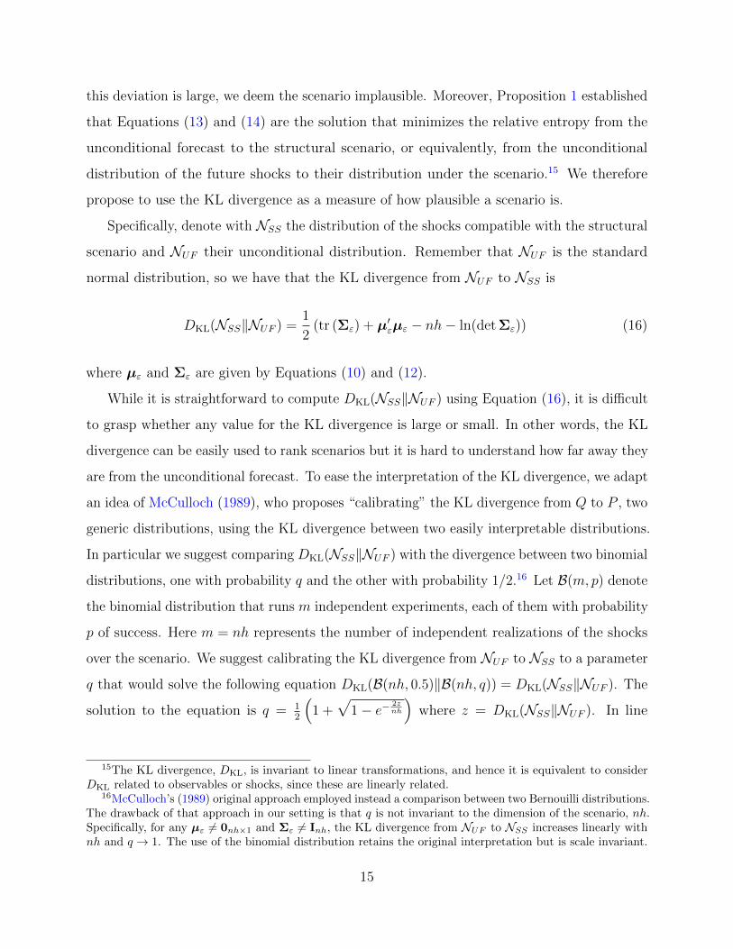
propose to use the KL divergence as a measure of how plausible a scenario is.
Specifically, denote with NSS the distribution of the shocks compatible with the structural
scenario and NUF their unconditional distribution. Remember that NUF is the standard
normal distribution, so we have that the KL divergence from NUF to NSS is
DKL(NSS‖NUF ) =1
2(tr (Σε) + µ′εµε − nh− ln(det Σε)) (16)
where µε and Σε are given by Equations (10) and (12).
While it is straightforward to compute DKL(NSS‖NUF ) using Equation (16), it is difficult
to grasp whether any value for the KL divergence is large or small. In other words, the KL
divergence can be easily used to rank scenarios but it is hard to understand how far away they
are from the unconditional forecast. To ease the interpretation of the KL divergence, we adapt
an idea of McCulloch (1989), who proposes “calibrating” the KL divergence from Q to P , two
generic distributions, using the KL divergence between two easily interpretable distributions.
In particular we suggest comparing DKL(NSS‖NUF ) with the divergence between two binomial
distributions, one with probability q and the other with probability 1/2.16 Let B(m, p) denote
the binomial distribution that runs m independent experiments, each of them with probability
p of success. Here m = nh represents the number of independent realizations of the shocks
over the scenario. We suggest calibrating the KL divergence from NUF to NSS to a parameter
q that would solve the following equation DKL(B(nh, 0.5)‖B(nh, q)) = DKL(NSS‖NUF ). The
solution to the equation is q = 12
(1 +
√1− e− 2z
nh
)where z = DKL(NSS‖NUF ). In line
15The KL divergence, DKL, is invariant to linear transformations, and hence it is equivalent to considerDKL related to observables or shocks, since these are linearly related.
16McCulloch’s (1989) original approach employed instead a comparison between two Bernouilli distributions.The drawback of that approach in our setting is that q is not invariant to the dimension of the scenario, nh.Specifically, for any µε 6= 0nh×1 and Σε 6= Inh, the KL divergence from NUF to NSS increases linearly withnh and q → 1. The use of the binomial distribution retains the original interpretation but is scale invariant.
15

with McCulloch’s (1989) original idea, any value for the KL divergence is translated into a
comparison between the flip of a fair and a biased coin. For example, a value of q = 0.501
suggests that the distribution of the shocks under the scenario considered is not at all far
from its unconditional counterpart, and the scenario considered is quite realistic. With a
value of q = 0.99 the restrictions imply a substantial deviation of the future shocks from their
unconditional distribution, suggesting that the scenario is quite unlikely.17
Our measure of plausibility is in the spirit of the concept of “modest intervention” used
in Leeper and Zha (2003). Their measure reports how unusual is the path for policy shocks
needed to achieve some conditional forecast, relative to the typical size of the shocks. If the
scenario implies a sequence of shocks close to their typical size, the intervention is considered
modest, and the results of the analysis are likely to be reliable. If instead the scenario involves
an unlikely sequence of shocks, Leeper and Zha (2003) argue that economic agents may alter
their behavior in meaningful ways and the analysis is deemed implausible.
Our metric compares the entire distribution rather than the path of the policy shocks,
and generalizes to scenarios other than those involving a single policy instrument and a single
policy shock.18 Moreover, an appealing feature of a metric based on the KL divergence is
that it provides an information-theoretical interpretation of the scenario, in terms of how
much information is added by the restrictions. If a scenario involves meaningful distortions
of the probability distribution of the underlying shocks, we should deem it as implausible
and the metric calls for caution about the use of the SVAR for this particular task.
4. Algorithms for implementation
In this section we briefly sketch a Bayesian algorithm for implementation of the gen-
eral framework above, which includes conditional-on-observables, conditional-on-shocks and
17In order to get a sense of how large is a specific calibration value, q, it might be useful to draw a parallelwith a standard IRF, in which only one shock is active, equal to 1 s.d. for one period, and zero otherwise.With, say, n = 8 and h = 12, and assuming Σε = Inh, we have q = 0.55, a very reasonable scenario. A large,but not unreasonable, 2 s.d. shock, leads instead to q = 0.6. Moreover, a sequence of 1 s.d. shocks over 12consecutive quarters leads to a q = 0.67, roughly equivalent to the q obtained from a single 3.5 standarddeviation shock. For an extremely large shock of 10 s.d. we get a q = 0.9.
18That Leeper and Zha (2003) compare the path of the policy shocks is a consequence of the fact thatthey set all other shocks to zero.
16

structural scenarios as special cases. In the interest of space, we describe the main features
here, relegating the technical details to the online Appendix. It should be clear that our
objective is to draw from the following joint posterior p(yT+1,T+h,A0,A+|yT , IR,SR) where
IR are the structural identification restrictions, and SR are the restrictions on the path of
future variables, shocks, or both. As explained by Waggoner and Zha (1999), drawing from
this posterior distribution is a challenging task. It is tempting, in a first step, to draw the
structural parameters from their distribution conditional on yT and on IR, and in a second
step to draw yT+1,T+h conditional on yT , on SR and on the structural parameters using
Equations (13) and (14). However, this procedure ignores the restrictions in Equation (15)
when drawing the structural parameters and, hence, would not lead to a draw from the desired
joint posterior. Instead, to draw from the joint distribution of interest, a Gibbs sampler
procedure must be constructed that iterates between draws from the described conditional
distributions of the structural parameters and yT+1,T+h in the following way
Algorithm 1. Initialize yT+h,(0) = [yT , y(0)T+1,T+h], e.g., at the mean unconditional forecast
1. Conditioning on yT+h,(i−1) = [yT , y(i−1)T+1,T+h], use any valid algorithm to produce one
draw from the structural parameters, (A(i)0 ,A
(i)+ ) satisfying IR.
2. Conditioning on (A(i)0 ,A
(i)+ ) and yT , draw y
(i)T+1,T+h ∼ N (µy,Σy) satisfying SR using
Equations (13) and (14).
3. Return to Step 1 until the convergence and a sufficient number of draws have been
obtained.
The algorithm above extends the one developed by Waggoner and Zha (1999), with the key
difference that we now need to identify the SVAR. For example, in the case of the traditional
recursive zero restrictions, Step 1 could draw the reduced-form coefficients and obtain A0
from the Cholesky decomposition of Σ. In the case of sign restrictions, Step 1 may be any of
the algorithms in Rubio-Ramirez et al. (2010) or Baumeister and Hamilton (2015). In the
cases of narrative sign restrictions (NSR) as in Antolin-Diaz and Rubio-Ramirez (2018) and
traditional sign and zero restrictions as in Arias et al. (2018), an importance-sampling step is
required to draw from the posterior of (A0,A+), which needs to be done at the end of Step 1.
17

4.1. The importance of using all available identification restrictions
When we use restrictions that set identify the model, the results of the structural scenario
analysis will be valid across a set of structural models that satisfy the restrictions. This
attractive feature will come at the cost of possibly wide confidence bands around the forecast.
Most importantly, there is the risk of including many models with implausible implications
for elasticities, structural parameters, shock realizations and historical decompositions.19 For
instance, in the applications with monetary policy shocks that we present below, we find that
a strategy based exclusively on traditional sign restrictions on IRFs often leads to implausibly
large elasticities of observable variables to a monetary policy shock, mirroring the results
of Kilian and Murphy (2012).20 In the examples, we will propose using a combination of
traditional sign and zero restrictions at various horizons, as in Arias et al. (2016), bounds on
elasticities, and the recently proposed NSR of Antolin-Diaz and Rubio-Ramirez (2018) to
narrow down the set of admissible structural parameters and obtain meaningful scenarios.
5. Application 1: Monetary policy and the power of forward guidance
Our first application concerns the effects of communicating future monetary policy shocks.
We provide new empirical estimates of the effects of anticipated monetary policy shocks,
compare alternative structural scenarios to the ones obtained with DSGE models, and evaluate
the potential of “makeup” strategies for inflation targeting.
Setup and identification. We work with the data set of Smets and Wouters (2007) (SW07),
which contains seven key US macroeconomic time series at quarterly frequency: real output,
consumption, investment, wages and hours worked per capita, inflation and the fed funds
rate. Their data set starts in Q1 1966; we update it through Q4 2019. In order to identify
anticipated monetary policy shocks, we will need a variable capturing changes in expectations
of future interest rates. We follow an approach similar to that of Campbell et al. (2012) and
19This point has been forcefully argued by Kilian and Murphy (2012), Ahmadi and Uhlig (2015), Ariaset al. (2016), Ludvigson et al. (2017) and Antolin-Diaz and Rubio-Ramirez (2018).
20These elasticities are much larger than the upper bound reported in Ramey’s (2016) literature review.These translate into explosive forecasts of the variables even for modest deviations of the conditioned variablefrom its unconditional path.
18

use expectations from the Survey of Professional Forecasters (SPF), available for the first
four quarters. Specifically, define as ESPFt [it+h] the mean SPF expectation at time t of the
short-term interest rate h quarters ahead. Then, the variable St,h ≡ ESPFt [it+h]− ESPF
t−1 [it+h]
for h = 0, . . . , 3 measures the surprise to expectations, i.e., the change in the information
set, from t− 1 to t. Campbell et al. (2012) point out that surprises across horizons h exhibit
a strong factor structure, so we take the average across horizons, St ≡ 1/4∑3
h=0 St,h as a
measure of the surprises to the average expected interest rate for the next year.21. After
appending St to the SW07 data set, we estimate an SVAR with p = 4 lags and an informative
“Minnesota” prior (Doan et al., 1986; Sims, 1993) over the reduced-form parameters.22 We
identify two orthogonal monetary policy shocks by means of the following restrictions.
Identification Restriction 1: (Unanticipated Monetary Policy Shocks) The unanticipated
monetary policy shock increases the fed funds rate on impact, decreases output, inflation,
consumption, investment, hours and wages on impact, and has zero impact on the level of
GDP in the long run, and a negative long-run impact on the price level. Moreover, it takes a
positive value in Q4 1979 and is the single largest contributor to the unexpected movement
in the fed funds rate in the same quarter. Finally, we restrict the maximum peak to trough
response of output to a 100bp monetary policy shock to 10 pp.
The traditional sign and zero restrictions are satisfied by standard New Keynesian models
such as Christiano et al. (1999) or SW07. The NSR follows Antolin-Diaz and Rubio-Ramirez
(2018) and is motivated by the historical account of the Volcker tightening. The bound on
the elasticity, set to twice the maximum amount reported by Ramey (2016), rules out models
in which very small changes in the interest rate lead to massive declines in output.
21Using instead the first principal component yields essentially identical results. In the online Appendix,we show that inclusion of this variable among the observables in a DSGE model featuring anticipated shocksis enough to guarantee invertibility of the VAR representation, and thus the ability to recover the structuralshocks from the reduced-form innovations (see Fernandez-Villaverde et al., 2007)
22See the online Appendix for exact definitions of the variables and prior.
19

Identification Restriction 2: (Anticipated Monetary Policy Shocks) The anticipated
monetary policy shock has the same sign effects on impact, zero long-run effects, and elastic-
ity bounds as the unanticipated shock. Additionally, the effect on the fed funds rate is positive
for the first three quarters, and it increases the surprise variable St on impact. Normalizing
for the size of the impact on the fed funds rate, the increase in St is larger than the one
caused by the unanticipated monetary policy shock. Finally, the anticipated monetary policy
shock satisfies the NSR in Table 1.
Consistent with the evidence that policy surprises are correlated across horizons, we aim to
identify a shock that affects the level of the interest rate over the next year, without imposing
zero impact of the anticipated shock on the contemporaneous fed funds rate.23 We derive the
restrictions above from the ones implied by introducing an equivalently defined anticipated
monetary policy shock within the SW07 DSGE model.24 The NSR improve the identification
by bringing in information about announcements made by the Federal Reserve in 2003 and
2011-2012.25 Notice that we only impose the sign of the shocks because our reading of
these events indicates that contemporaneous news about growth and inflation may have also
influenced the announcements. We wish to stress that in general the surprise variable St
is almost certainly affected in any quarter by many other shocks. Therefore, it would not
constitute a valid instrument for anticipated monetary policy shocks. The advantage of the
NSR approach in this context is that it allows us to incorporate the information that these
shocks were affecting expectations during specific events.
For the results that follow it will be useful to also identify an “aggregate demand” shock,
which generates positive co-movement between interest rates and business cycle variables.
23In our setting, an announcement of future actions with no contemporaneous change in the policy rate isbest thought of as a combination of anticipated and unanticipated shocks
24Specifically, we introduce an anticipated monetary policy shock to the central bank reaction function inline with Campbell et al. (2012) and Campbell et al. (2017). The monetary policy ‘news’ shock obeys a simplefactor structure for the first four quarters that embodies the idea that forward guidance is characterized byan announcement of a persistent deviation from the usual conduct of policy. Full details are available in theonline Appendix.
25A motivation based on FOMC statements, minutes and transcripts is provided in the online Appendix.
20

Table 1: Summary of Forward Guidance FOMC Statement Language
Economic Conditions Language NSRGrowth Inflation
Q3 2003 “upside and downside risks [...] “risk of inflation becoming “policy accommodation can be maintained −roughly equal” undesirably low” for a considerable period”
Q1 2004 “upside and downside risks [...] “probability of an unwelcome fall[...] “patient in removing +roughly equal” almost equal to that of a rise” its policy accommodation”
Q2 2004 “upside and downside risks [...] “risks to [...] price stability “policy accommodation can be removed −roughly equal” moved into balance” at a pace that is likely to be measured”
Q3 2011 “Considerably slower” “picked up” “low levels warranted at −least through mid 2013”
Q1 2012 “expanding moderately” “at or below mandate” “low levels warranted at −least through late 2014”
Q3 2012 “moderate pace” “subdued” “at least through mid 2015” −
Identification Restriction 3: (Aggregate Demand Shocks) The aggregate demand shock
has a positive effect on impact on output, consumption, investment, hours, wage, inflation
and the fed funds rate, and zero long-run impact on the level of GDP.
Figure 2 displays the IRFs of key variables to the two policy shocks.26 While the effects of the
two shocks are quite similar, normalizing for the peak effect on the fed funds rate, the impact
of the anticipated shock on output and inflation is somewhat larger and more persistent.
The SVAR results do not display the “forward guidance puzzle” reported by Del Negro et al.
(2012), and McKay et al. (2016), who find unrealistically large effects of anticipated shocks
using DSGE models. We will expand on the reasons for this difference below.
Structural Scenario 1: Delphic vs. Odyssean forward guidance. The first of our exercises
considers the two alternative questions we referred to in the introduction, the results of
which we anticipated in Figure 1. In particular, we consider an exercise that might have
been contemplated by the FOMC at the end of 2019. After three consecutive 25-basis-point
cuts in previous meetings, the FOMC decided to keep the fed funds rate at a range of 1.5
to 1.75%. What if the FOMC had at this point announced a further reduction to 1%, after
26The IRFs of the remaining variables and shocks are displayed in the online Appendix.
21

Figure 2: Monetary Policy: Impulse Response Functions to anticipated vs unanticipatedshocks
0 5 10 15 20
Quarters
0
1
2
3
0 5 10 15 20
Quarters
-0.1
0
0.1
0.2
0.3
0 5 10 15 20
Quarters
-0.6
-0.4
-0.2
0
0.2
0.4
0 5 10 15 20
Quarters
-0.3
-0.2
-0.1
0
0.1
0.2
Note: The blue (lighter) shaded area represents the 68% (point-wise) HPD credible sets for the IRFs andthe blue dotted lines are the median IRFs to an expansionary unanticipated monetary policy shock of onestandard deviation. The red (darker) shaded areas and red solid lines display the equivalent quantities forthe anticipated policy shock.
which the policy rate would be held constant for two years? In terms of our framework, this
“dovish” scenario can be implemented as a restriction on the path of future observables using
Equation (5). But whether we frame it in terms of a conditional-on-observables forecast
or a structural scenario will yield completely different answers. Figure 3 illustrates this
point by comparing the unconditional distribution of the three identified shocks in the first
period of the forecast to the one resulting from several conditional-on-observables forecast
and structural scenario exercises. As we can see in Panel (a), the conditional-on-observables
exercise involves contractionary demand shocks generating, through the systematic reaction
of the central bank, a positive co-movement between inflation and interest rates. As a result,
output and inflation are weak. In this sense the exercise is at least partially Delphic. There
are many occasions in which this setting may not be appropriate. For instance, in September
2012 the FOMC announced it expected to keep interest rates constant until mid-2015. The
minutes of the meeting make clear that
“[the] new language was meant to clarify that the maintenance of a very low fed
22

Figure 3: Distribution of Shocks Underlying Different Exercises
(a) Conditional-on-Observables Forecast
MP Shock
-4 -2 0 2 40
0.05
0.1
0.15
0.2
0.25
0.3
0.35
0.4
0.45
0.5AMP Shock
-4 -2 0 2 40
0.05
0.1
0.15
0.2
0.25
0.3
0.35
0.4
0.45
0.5AD Shock
-4 -2 0 2 40
0.05
0.1
0.15
0.2
0.25
0.3
0.35
0.4
0.45
0.5
(b) An Odyssean Scenario
MP Shock
-4 -2 0 2 40
0.05
0.1
0.15
0.2
0.25
0.3
0.35
0.4
0.45
0.5AMP Shock
-4 -2 0 2 40
0.05
0.1
0.15
0.2
0.25
0.3
0.35
0.4
0.45
0.5AD Shock
-4 -2 0 2 40
0.05
0.1
0.15
0.2
0.25
0.3
0.35
0.4
0.45
0.5
(c) A Delphic Scenario
MP Shock
-4 -2 0 2 40
0.05
0.1
0.15
0.2
0.25
0.3
0.35
0.4
0.45
0.5AMP Shock
-4 -2 0 2 40
0.05
0.1
0.15
0.2
0.25
0.3
0.35
0.4
0.45
0.5AD Shock
-4 -2 0 2 40
0.05
0.1
0.15
0.2
0.25
0.3
0.35
0.4
0.45
0.5
Note: For each panel, the gray shaded area represents the probability density function (p.d.f.) of a standardnormal distribution, whereas the broken blue line is the p.d.f. of the different shocks at horizon h = 1 forthe three variants of the “dovish” scenario. MP stands for unanticipated monetary policy shocks, AMP foranticipated monetary policy shocks, and AD for aggregate demand shocks.
23

funds rate over that period did not reflect an expectation that the economy would
remain weak, but rather reflected the Committee’s intention to support a stronger
economic recovery.”27
We make this idea operational with a scenario in which all non-policy shocks are restricted
to retain their unconditional distributions. By doing so, we avoid inferring anything about
future demand and supply shocks from the lower path of interest rates. The results for the
path of output and inflation are visible in Panel (b) of Figure 1, and for the associated shocks
in Panel (b) of Figure 3. As we can see, there is a moderate boom in output, and inflation is
slightly above the unconditional forecast. In the conditional-on-observables forecast, monetary
policy shocks also played a role, reflecting the likelihood that at least some movements in
interest rates represent exogenous policy actions. In that sense it mixes Delphic and Odyssean
content. Can we construct a strictly Delphic scenario? The answer is yes. We create a
Delphic variant of the scenario by restricting the two policy shocks to their unconditional
distribution, leaving all other shocks unconstrained. The results can be seen in Figure 4 and
the associated distribution of first period shocks is in Panel (c) of Figure 3. Output and
inflation are now even lower than in the conditional-on-observables forecast, since we are
shutting down the possibility that expansionary monetary policy shocks play any role.
The importance of quantifying uncertainty. In the scenarios above we fixed the path for
the fed funds rate with zero uncertainty, i.e., Ωf = 0ko×ko , as has been traditional in the
literature. As pointed out by Andersson et al. (2010), this will lead to a reduction in the
variance of the conditional forecast relative to the unconditional forecast. Instead, when one
wants to preserve the uncertainty present in the unconditional forecast, the variance around
the fed funds rate can be set to Ωf = DD′, as proposed in Section 2.2. In the monetary
policy example, this has an interesting economic interpretation. When fixing the policy
instrument to a particular path, the scenario can be interpreted as an ironclad commitment:
the monetary policy will follow that path no matter what the realizations of the other shocks
27Emphasis ours. See “Minutes of the Federal Open Market Committee” September 12-13, 2012 (ReleasedOctober 4, 2012). https://www.federalreserve.gov/monetarypolicy/fomcminutes20120913.htm
24

Figure 4: A Delphic Scenario
GDP per cap. growth
2016 2017 2018 2019 2020 2021-0.5
0
0.5
1
1.5
2
2.5
3
3.5
4
% p
.a. (
4-qu
arte
r av
erag
e)
Core PCE inflation
2016 2017 2018 2019 2020 20210
0.5
1
1.5
2
2.5
% p
.a. (
4-qu
arte
r av
erag
e)
Federal Funds Rate
2016 2017 2018 2019 2020 20210
0.5
1
1.5
2
2.5
3
% p
.a.
Note: For each panel, the solid black lines represent actual data, the solid red line is the conditioningassumption on the fed funds rate, the solid blue line is the median forecast for the remaining variables andperiods, and the blue shaded areas denote the 40 and 68% pointwise credible sets around the forecasts. Thedotted gray lines represent the median unconditional forecast.
are. If instead uncertainty about the fed funds path is recognized, the exercise acquires the
flavor of a “data dependent” commitment.
If one further imposed that the “non-driving” shocks are equal to zero, i.e., Ωg = 0ks ,
an even greater reduction in the variance of the forecast would result.28 Intuitively, this
assumption implies that the forecaster has knowledge that these shocks will not occur. As a
result, the forecast density produced will greatly underestimate the underlying uncertainty
about the future. Instead, by setting their distribution equal to the unconditional distribution,
i.e., Ωg = Iks we take the position of a forecaster who possesses no additional knowledge
(over the unconditional forecast) about the “non-driving” shocks. Ignoring these two sources
of uncertainty may make the results implausible and substantially less useful, particularly
if one is interested in density forecasting. To illustrate this point, Table 2 reports, for the
Odyssean variant of Scenario 1, the plausibility metric from Section 3 and a number of risk
28This is the implicit assumption of existing methodologies, including Leeper and Zha (2003), Baumeisterand Kilian (2014), and Banbura et al. (2015). A figure displaying the consequences of the alternativetreatments of uncertainty for the density forecasts for this exercise is available in the online Appendix.
25
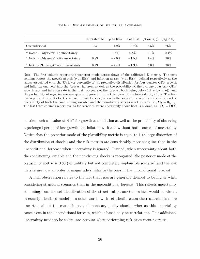
Table 2: Risk Assessment of Structural Scenarios
Calibrated KL g at Risk π at Risk p(low π, g) p(g < 0)
Unconditional 0.5 −1.2% −0.7% 6.5% 26%
“Dovish - Odyssean” no uncertainty 1 1.8% 0.8% 0.1% 0.4%
“Dovish - Odyssean” with uncertainty 0.83 −2.0% −1.5% 7.4% 26%
“Back to PL Target” with uncertainty 0.73 −2.4% −1.3% 5.0% 36%
Note: The first column reports the posterior mode across draws of the calibrated K metric. The nextcolumns report the growth-at-risk (g at Risk) and inflation-at-risk (π at Risk), defined respectively as thevalues associated with the 5% lower percentile of the predictive distribution for four-quarter GDP growthand inflation one year into the forecast horizon, as well as the probability of the average quarterly GDPgrowth rate and inflation rate in the first two years of the forecast both being below 1%(p(low π, g)), andthe probability of negative average quarterly growth in the third year of the forecast (p(g < 0)). The firstrow reports the results for the unconditional forecast, whereas the second row reports the case when theuncertainty of both the conditioning variable and the non-driving shocks is set to zero, i.e., Ωf = 0ko×ko .The last three columns report results for scenarios where uncertainty about both is allowed, i.e., Ωf = DD′.
metrics, such as “value at risk” for growth and inflation as well as the probability of observing
a prolonged period of low growth and inflation with and without both sources of uncertainty.
Notice that the posterior mode of the plausibility metric is equal to 1 (a large distortion of
the distribution of shocks) and the risk metrics are considerably more sanguine than in the
unconditional forecast when uncertainty is ignored. Instead, when uncertainty about both
the conditioning variable and the non-driving shocks is recognized, the posterior mode of the
plausibility metric is 0.83 (an unlikely but not completely implausible scenario) and the risk
metrics are now an order of magnitude similar to the ones in the unconditional forecast.
A final observation relates to the fact that risks are generally deemed to be higher when
considering structural scenarios than in the unconditional forecast. This reflects uncertainty
stemming from the set identification of the structural parameters, which would be absent
in exactly-identified models. In other words, with set identification the researcher is more
uncertain about the causal impact of monetary policy shocks, whereas this uncertainty
cancels out in the unconditional forecast, which is based only on correlations. This additional
uncertainty needs to be taken into account when performing risk assessment exercises.
26

Structural Scenario 2: Evaluating forward guidance in the time of Greenspan. Our next
exercise considers the difference between anticipated and unanticipated monetary shocks in
more detail, and compares the results of our approach to the ones that would be obtained
with the workhorse SW07 DSGE model. In particular, we examine the tightening cycle of
2004-2006, noteworthy for the fact that, in the prior year, the FOMC had been experimenting
with forward guidance about the future path of interest rates. To simulate a real-time exercise
we re-estimate our SVAR model using the vintage of data ending in Q4 2004, the original
data set used by SW07.29 For the DSGE model we fix the parameters to the posterior
modal estimates reported by Smets and Wouters and introduce an anticipated monetary
policy shock that is consistent with our identification strategy above and construct equivalent
scenarios.30 In Q3 2004, the FOMC initiated a tightening sequence that increased the fed
funds rate by 25-basis-points each meeting until reaching 5.25%. What if instead the FOMC
had decided to postpone that process by one year, keeping interest rates constant until then
using policy shocks? How would the results differ depending on whether such an action was
communicated in advance? Figure 5 compares the answers obtained using our SVAR and the
DSGE model. Panel (a) implements this scenario only through unanticipated shocks. As we
can see, the results of the SVAR are very similar to the point estimates from the DSGE model,
though the effect on inflation appears slightly more front loaded. As we can see in Panel (b),
things are more different in the case in which anticipated shocks are included. Using New
Keynesian DSGE models, Del Negro et al. (2012) and McKay et al. (2016) find responses to
anticipated policy shocks that are unrealistically large, and become even larger the longer
the horizon of anticipation. The SVAR instead finds that the differences between anticipated
and unanticipated policies are relatively minor.31 Moreover, in the present exercise, since the
horizon of anticipation spans only the first four quarters, we observe only a modest forward
29To identify the shocks, we only use the NSR up to Q2 2004.30Since the SW07 model does not have a VAR representation, we cannot apply Equations (10)-(14) or
algorithm 1 directly to compute the scenarios for the DSGE model. However, conditioning on the parameters,we can use the state-space representation of the model and the Kalman filter to compute the mean of thescenario. For this reason we only report point estimates for the SW07 model.
31The plausibility metric is 0.84 in the case where anticipation is allowed, and 0.8 when it is not, indicatingthat such exercises already imply a meaningful divergence from the unconditional distribution.
27

guidance puzzle with the DSGE, and the results are similar to the ones obtained with the
SVAR. For scenarios that envision more drastic deviations from the unconditional forecast, or
actions expanding into more distant horizons, however, the differences can become very large.
Our empirical results provide a useful benchmark for any theoretical developments that aim
to solve the forward guidance puzzle. The exercise also highlights one of the main practical
motivations behind our paper: the scenarios conducted with DSGE models can be sensitive
to the details of the model assumptions, whereas the ones constructed with SVARs will be
consistent with a set of incompletely specified and not fully trusted models. When one is
uncertain about which underlying structural model to use, our methodology will constitute a
pragmatic alternative.
Structural Scenario 3: Returning to the price level target. Our final exercise considers a
different thought experiment. Since the FOMC announced a 2% inflation target in January
2012, the average rate of inflation as measured by the PCE deflator excluding food and energy
turned out to be 1.6%, resulting in a 4% cumulative shortfall relative to a hypothetical price
level target by the end of 2019. The possibility of adopting a “makeup” strategy that would
aim to revert the past shortfall has been widely discussed in policy circles in recent years.32
What distribution of policy shocks would be required going forward to return to the 2% price
level target, say, within 5 years? It is straightforward to implement this question using our
structural scenario framework where only the two policy shocks are allowed to deviate from
their unconditional distribution. Suppose that inflation is the i-th variable in the system
and that one wanted to eliminate a cumulative shortfall of π over h periods. We can write
this restriction as 1/h∑h
s=1 yi,t+s ∼ N (2+π/h, ωf ). The restriction states that the average
inflation over the forecast horizon needs to be, in expectation, above the 2% target by π/h
every period in order to eliminate the past accumulated inflation shortfall, with variance
ωf . Notice that our methodology is flexible enough that we do not need to input a specific
path of inflation. Our method will yield the distribution of future policy shocks that is
consistent with the smallest deviation from their unconditional distribution while satisfying
32See, e.g., Bernanke (2017). Those “makeup” strategies are also discussed within the Federal Reserve“Review of Monetary Policy Strategy, Tools, and Communication Practices;” see, e.g., Clarida (2019).
28

Figure 5: Comparison of SVAR and DSGE results
(a) Unanticipated Shocks Only
GDP per cap. growth
2001 2002 2003 2004 2005 2006 2007 2008-4
-2
0
2
4
6
8
% p
.a. (
4-qu
arte
r av
erag
e)
Core PCE inflation
2001 2002 2003 2004 2005 2006 2007 20080
1
2
3
4
5
6
7
8
% p
.a. (
4-qu
arte
r av
erag
e)
Federal Funds Rate
2001 2002 2003 2004 2005 2006 2007 20080
1
2
3
4
5
6
7
8
% p
.a.
(b) Anticipated and Unanticipated Shocks
GDP per cap. growth
2001 2002 2003 2004 2005 2006 2007 2008-4
-2
0
2
4
6
8
% p
.a. (
4-qu
arte
r av
erag
e)
Core PCE inflation
2001 2002 2003 2004 2005 2006 2007 20080
1
2
3
4
5
6
7
8
% p
.a. (
4-qu
arte
r av
erag
e)
Federal Funds Rate
2001 2002 2003 2004 2005 2006 2007 20080
1
2
3
4
5
6
7
8
% p
.a.
Note: For each panel, the solid black lines represent actual data. In the third column, the solid red lineand associated shaded areas are the median, 40 and 68% pointwise credible sets around the conditioningassumptions for the fed funds rate. In the first and second panels, the solid blue line and associated shadedareas are the median, 40 and 68% pointwise credible sets around the forecasts of the other variables given bythe SVAR. The dotted gray lines represent the median unconditional forecast from the SVAR. The brokenblack lines represent instead the mean results obtained using the DSGE model of SW07.
the restriction on 1/h∑h
s=1 yi,t+s. Moreover, the interest rate distribution we obtain will be
the one that “makes up” for the past inflation shortfall with the smallest deviation from the
usual policy rule. The results can be seen in Figure 6. Inflation needs to increase gradually,
peaking at 2.9% in mid-2023, before returning to the 2% target. In order to achieve the
inflation, the fed funds rate is cut to about 1.3%, after which it starts increasing rapidly,
until reaching 4% in 2023. This large tightening is required to cool down the boom in output
29

and inflation triggered by the new policy and bring inflation back to target. Using a car
analogy, to catch up a car ahead of you that goes as fast as you, one needs to accelerate first
and then decelerate. Decelerating the pace of price increases, requires higher interest rates to
weaken aggregate demand. The results for output highlight a clear risk: while the price level
successfully returns to the target, the subsequent tightening implies meaningful probabilities
(around 46%) of negative annual growth in the fourth and fifth years of the sample. If the
return to the price level target would be executed over a longer period, the implied slowdown
would be less pronounced. Interestingly, this scenario produces larger effects on output and
inflation than the apparently more aggressive interest rate cuts of Scenario 1. The reason is
that Scenario 3 involves a greater share of anticipated monetary policy shocks relative to
Scenario 1, which included a large unanticipated movement in the first period. As reported
in Table 2, the plausibility metric for this scenario has a posterior mode of 0.73, suggesting
it is a much more likely scenario than Scenario 1. Our results are consistent with policy
communication being an effective way to achieve the central bank’s objectives.33
6. Application 2: Stress-testing the response of asset prices to a recession
Our second application studies the impact of an economic recession on asset prices and
bank profitability. We highlight that the potential impact of a recessionary episode can be
very different depending on the shock driving it. Specifically, we will show how a recession
caused by financial shocks, like the one of 2007-09, can have a more damaging impact on bank
profitability (and other financial variables) than recessions driven by other types of shocks. We
augment the macro data set from the previous application by adding the unemployment rate,
as well as a number of financial variables: the 3-month Treasury bill to 10-year government
bond yield spread, the quarterly change in the S&P 500 stock price index, the quarterly
change in the S&P Case-Shiller House Price Index, the real price of oil, the BAA credit
spread, the 3-month Treasury bill-eurodollar (TED) spread; and an indicator of profitability
33Two alternative scenarios are presented in the online Appendix. The first considers returning to theprice level target over ten years instead of five. The second one features only unanticipated shocks. Theresults of the latter indicate that a more volatile interest rate path and a higher probability of recession wouldbe required to achieve the same objective.
30

Figure 6: Returning to the Price Level Target
GDP per cap. growth
2004 2006 2008 2010 2012 2014 2016 2018 2020 2022 2024-6
-4
-2
0
2
4
6
% p
.a. (
4-qu
arte
r av
erag
e)
Core PCE inflation
2004 2006 2008 2010 2012 2014 2016 2018 2020 2022 2024-2
-1
0
1
2
3
4
5
6
% p
.a. (
4-qu
arte
r av
erag
e)
Federal Funds Rate
2004 2006 2008 2010 2012 2014 2016 2018 2020 2022 20240
1
2
3
4
5
6
% p
.a.
Log Price Level
2004 2006 2008 2010 2012 2014 2016 2018 2020 2022 2024
90
100
110
120
130
Inde
x (2
012
Q1
= 1
00)
Note: For each panel, the solid black lines represent actual data. The solid blue lines and associated shadedareas are the median, 40 and 68% pointwise credible sets around the forecasts of the other variables givensuch that the constraint that the price level returns to the target within a five-year horizon is satisfied. Thedotted gray lines represent the median unconditional forecast.
in the banking system as a whole, the return on equity (ROE) of FDIC-insured institutions.34
Sample is from Q1 1966 to Q4 2019. We identify a single financial shock that resembles the
one at work during the last recession through the following combination of traditional and
narrative sign restrictions:
Identification Restriction 1: (Financial Shock) The financial shock has a negative impact
on stock prices and bank profitability, and increases the BAA and TED spreads. Moreover,
the financial shock for the observation corresponding to the fourth quarter of 2008 must be
of positive value and be the overwhelming driver of the unexpected movement in the TED
spread and credit spread.
34See the online Appendix for the definition of the variables and details of the model’s specification.
31

The NSR are based on the account in Bernanke (2015), which highlights how the collapse
of Lehman Brothers on September 13, 2008 caused “short-term lending markets to freeze
and increase the panicky hoarding of cash” (p. 268), “fanned the flames of the financial
panic” (p. 269), “directly touched off a run on money market funds” (p. 405), and “triggered
a large increase in spreads” (p. 405). The construction of the scenarios borrows from the
Federal Reserve’s “2019 Supervisory Scenarios for Annual Stress Tests Required under the
Dodd-Frank Act Stress Testing Rules and the Capital Plan Rule.”35 We take the path of
GDP and the unemployment rate described in the Fed’s “adverse scenario.” It describes a
medium-sized recession in which output falls for five consecutive quarters and then recovers
gradually, whereas the unemployment rate increases until it reaches 7%. As before, we
consider uncertainty around the path of the conditioning variables by setting Ωf = DD′.
Conditional on the restrictions for GDP and unemployment, we consider two distinct scenarios.
In the first, the recession is caused by a financial shock. This is achieved by restricting all
shocks except the financial one to their unconditional distribution. The second scenario is a
recession not driven by the financial shock. To implement this, we restrict the financial shock
to retain its unconditional distribution, and allow all the other shocks to deviate from theirs.
Figures 7 and 8 compare the results. The financial recession has a much more severe
impact on stock prices, credit spreads and bank profitability. Moreover, the impact of the oil
price is of opposite sign, indicating that non-financial recessions are often associated with
increases in oil prices. As for the plausibility of the exercise, for the non-financial recession,
the posterior mode of the calibrated KL measure is 0.68, whereas for the financial recession it
is 0.86. We interpret this result as reflecting the fact that in the sample, financial recessions
are a relatively infrequent event, and most postwar recessions appear to have involved a
mixture of non-financial factors. Therefore, these results based on relatively infrequent events
should be interpreted with caution. The results of this section highlight that if the scenario
is driven by a financial shock, even mild contractions in economic activity can result in large
damage to banks’ balance-sheet variables.
35See https://www.federalreserve.gov/newsevents/pressreleases/files/bcreg20190213a1.pdf
downloaded on January, 31, 2020.
32

Figure 7: A Stress Test Driven by a Financial Shock
GDP per cap. growth
2005 2010 2015 2020-6
-4
-2
0
2
4
6
% p
.a. (
4-qu
arte
r av
erag
e)
Unemployment Rate
2005 2010 2015 2020
4
6
8
10
12
% o
f la
bor
forc
e
Core PCE inflation
2005 2010 2015 20200
1
2
3
4
% p
.a. (
4-qu
arte
r av
erag
e)
S\&P 500 Stock Price Index
2005 2010 2015 2020-200
0
200
400
600
Log
arith
m
Case-Shiller Home Price Index
2005 2010 2015 2020-15
-10
-5
0
5
10
15
% p
.a. (
4-qu
arte
r av
erag
e)
WTI Crude Oil price
2005 2010 2015 2020-50
0
50
100
150
Log
arith
m
TED Spread
2005 2010 2015 20200
1
2
3
% p
.a.
BAA Spread
2005 2010 2015 20201
2
3
4
5
% p
.a.
Return on Equity
2005 2010 2015 2020-10
0
10
20
% p
.a.
Note: For each panel, the solid black lines represent actual data. In the first two panels, the solid red lineand associated shaded areas are the median, 40 and 68% pointwise credible sets around the conditioningassumptions for GDP growth and the unemployment rate. In the remaining panels, the solid blue line andassociated shaded areas are the median, 40 and 68% pointwise credible sets around the forecasts of the othervariables. The dotted gray lines represent the median unconditional forecast.
7. Conclusion
We have provided a general and flexible framework to construct structural scenarios based
on minimalistically identified VARs, paying close attention to the uncertainty stemming from
estimation, identification, and future shocks. While there will always be limits to the kinds
of experiments that can be performed on linear Gaussian models, we hope that our methods
facilitate a middle ground between relying on empirical models, which remain silent about
the underlying causal mechanisms, and committing to the specific details of a particular
structural model, which will give sharper, but surely misspecified answers.
References
Aastveit, K. A., A. Carriero, T. E. Clark, and M. Marcellino (2017): “Have standard VARsremained stable since the crisis?” Journal of Applied Econometrics, 32, 931–951.
33

Figure 8: A Stress Test Driven by Non-Financial Shocks
GDP per cap. growth
2005 2010 2015 2020-6
-4
-2
0
2
4
6
% p
.a. (
4-qu
arte
r av
erag
e)
Unemployment Rate
2005 2010 2015 2020
4
6
8
10
12
% o
f la
bor
forc
e
Core PCE inflation
2005 2010 2015 20200
1
2
3
4
% p
.a. (
4-qu
arte
r av
erag
e)
S\&P 500 Stock Price Index
2005 2010 2015 2020-200
0
200
400
600
Log
arith
m
Case-Shiller Home Price Index
2005 2010 2015 2020-15
-10
-5
0
5
10
15
% p
.a. (
4-qu
arte
r av
erag
e)
WTI Crude Oil price
2005 2010 2015 2020-50
0
50
100
150
Log
arith
m
TED Spread
2005 2010 2015 20200
1
2
3
% p
.a.
BAA Spread
2005 2010 2015 20201
2
3
4
5
% p
.a.
Return on Equity
2005 2010 2015 2020-10
0
10
20
% p
.a.
Note: For each panel, the solid black lines represent actual data. In the first two panels, the solid red lineand associated shaded areas are the median, 40 and 68% pointwise credible sets around the conditioningassumptions for GDP growth and the unemployment rate. In the remaining panels, the solid blue line andassociated shaded areas are the median, 40 and 68% pointwise credible sets around the forecasts of the othervariables. The dotted gray lines represent the median unconditional forecast.
Ahmadi, P. A. and H. Uhlig (2015): “Sign Restrictions in Bayesian FaVARs with an Application toMonetary Policy Shocks,” NBER Working Papers 21738, National Bureau of Economic Research, Inc.
Altavilla, C., D. Giannone, and M. Lenza (2016): “The Financial and Macroeconomic Effects of theOMT Announcements,” International Journal of Central Banking, 12, 29–57.
Andersson, M. K., S. Palmqvist, and D. F. Waggoner (2010): “Density Conditional Forecasts inDynamic Multivariate Models,” Sveriges Riksbank Working Paper Series 247, Sveriges Riksbank.
Antolin-Diaz, J. and J. F. Rubio-Ramirez (2018): “Narrative Sign Restrictions for SVARs,” AmericanEconomic Review, 108, 2802–29.
Arias, J. E., D. Caldara, and J. F. Rubio-Ramirez (2016): “The Systematic Component of MonetaryPolicy in SVARs: An Agnostic Identification Procedure,” International Finance Discussion Papers 1131,Board of Governors of the Federal Reserve System (U.S.).
Arias, J. E., J. F. Rubio-Ramirez, and D. F. Waggoner (2018): “Inference Based on SVARs Identifiedwith Sign and Zero Restrictions: Theory and Applications,” Econometrica, 86, 685–720.
Banbura, M., D. Giannone, and M. Lenza (2015): “Conditional forecasts and scenario analysis withvector autoregressions for large cross-sections,” International Journal of Forecasting, 31, 739–756.
34

Baumeister, C. and J. D. Hamilton (2015): “Sign restrictions, structural vector autoregressions, anduseful prior information,” Econometrica, 83, 1963–1999.
Baumeister, C. and L. Kilian (2014): “Real-Time Analysis of Oil Price Risks Using Forecast Scenarios,”IMF Economic Review, 62, 119–145.
Ben-israel, A. and T. N. E. Greville (2001): Generalized Inverses: Theory and Applications, Springer-Verlag New York, second ed.
Bernanke, B. S. (2015): The Courage to Act, W.W. Norton & Company.
——— (2017): “Monetary Policy in a New Era,” Tech. rep., Peterson Institute for International Economics.
Bernanke, B. S., M. Gertler, and M. Watson (1997): “Systematic Monetary Policy and the Effects ofOil Price Shocks,” Brookings Papers on Economic Activity, 28, 91–157.
Campbell, J. R., C. L. Evans, J. D. Fisher, and A. Justiniano (2012): “Macroeconomic Effects ofFederal Reserve Forward Guidance,” Brookings Papers on Economic Activity, 43, 1–80.
Campbell, J. R., J. D. Fisher, A. Justiniano, and L. Melosi (2017): “Forward guidance andmacroeconomic outcomes since the financial crisis,” NBER Macroeconomics Annual, 31, 283–357.
Christiano, L. J., M. Eichenbaum, and C. L. Evans (1999): “Monetary policy shocks: What havewe learned and to what end?” in Handbook of Macroeconomics, ed. by J. B. Taylor and M. Woodford,Elsevier, vol. 1 of Handbook of Macroeconomics, chap. 2, 65–148.
Clarida, R. H. (2019): “The Federal Reserve’s Review of Its Monetary Policy Strategy, Tools, andCommunication Practices,” Speech, At “A Hot Economy: Sustainability and Trade-Offs,” a Fed Listensevent sponsored by the Federal Reserve Bank of San Francisco, San Francisco, California.
Clarida, R. H. and D. Coyle (1984): “Conditional Projection by Means of Kalman Filtering,” NBERTechnical Working Papers 0036, National Bureau of Economic Research, Inc.
Clark, T. E. and M. W. McCracken (2014): “Evaluating Conditional Forecasts from Vector Autoregres-sions,” Working Paper 1413, Federal Reserve Bank of Cleveland.
Conti, A. M., A. Nobili, F. M. Signoretti, et al. (2018): “Bank capital constraints, lending supplyand economic activity,” Tech. rep., Bank of Italy, Economic Research and International Relations Area.
Del Negro, M., M. P. Giannoni, and C. Patterson (2012): “The forward guidance puzzle,” FRB ofNew York Staff Report.
Del Negro, M. and F. Schorfheide (2013): DSGE Model-Based Forecasting, Elsevier, vol. 2A of Handbookof Economic Forecasting, chap. 2, 57–140.
Doan, T., R. B. Litterman, and C. A. Sims (1986): “Forecasting and conditional projection usingrealistic prior distribution,” Staff Report 93, Federal Reserve Bank of Minneapolis.
Fernandez-Villaverde, J., J. F. Rubio-Ramırez, T. J. Sargent, and M. W. Watson (2007): “ABCs(and Ds) of Understanding VARs,” American Economic Review, 97, 1021–1026.
Giacomini, R. and G. Ragusa (2014): “Theory-coherent forecasting,” Journal of Econometrics, 182,145–155.
Giannone, D., M. Lenza, D. Momferatou, and L. Onorante (2014): “Short-term inflation projections:a Bayesian vector autoregressive approach,” International Journal of Forecasting, 30, 635–644.
35

Giannone, D., M. Lenza, H. Pill, and L. Reichlin (2012): “The ECB and the interbank market,” TheEconomic Journal, 122, F467–F486.
Giannone, D., M. Lenza, and L. Reichlin (2019): “Money, Credit, Monetary Policy, and the BusinessCycle in the Euro Area: What Has Changed Since the Crisis?” International Journal of Central Banking,15, 137–173.
Hamilton, J. D. and A. M. Herrera (2004): “Oil Shocks and Aggregate Macroeconomic Behavior: TheRole of Monetary Policy: Comment,” Journal of Money, Credit and Banking, 36, 265–286.
Jarocinski, M. (2010): “Conditional forecasts and uncertainty about forecast revisions in vector autoregres-sions,” Economics Letters, 108, 257–259.
Kilian, L. and L. T. Lewis (2011): “Does the Fed Respond to Oil Price Shocks?” Economic Journal, 121,1047–1072.
Kilian, L. and S. Manganelli (2008): “The central banker as a risk manager: Estimating the FederalReserve’s preferences under Greenspan,” Journal of Money, Credit and Banking, 40, 1103–1129.
Kilian, L. and D. P. Murphy (2012): “Why agnostic sign restrictions are not enough: Understanding thedynamics of oil market VAR models,” Journal of the European Economic Association, 10, 1166–1188.
Leeper, E. M., C. A. Sims, and T. Zha (1996): “What does monetary policy do?” Brookings Papers onEconomic Activity, 1996, 1–78.
Leeper, E. M. and T. Zha (2003): “Modest policy interventions,” Journal of Monetary Economics, 50,1673–1700.
Lucas, R. E. (1976): “Econometric policy evaluation: A critique,” in Carnegie-Rochester Conference Serieson Public Policy, vol. 1, 19–46.
Ludvigson, S. C., S. Ma, and S. Ng (2017): “Shock Restricted Structural Vector-Autoregressions,” NBERWorking Papers 23225, National Bureau of Economic Research, Inc.
McCulloch, R. E. (1989): “Local Model Influence,” Journal of the American Statistical Association, 84,473–478.
McKay, A., E. Nakamura, and J. Steinsson (2016): “The power of forward guidance revisited,”American Economic Review, 106, 3133–58.
Penrose, R. (1955): “A generalized inverse for matrices,” Mathematical Proceedings of the CambridgePhilosophical Society, 51, 406–413.
——— (1956): “On best approximate solutions of linear matrix equations,” Mathematical Proceedings of theCambridge Philosophical Society, 52, 17–19.
Ramey, V. A. (2016): “Macroeconomic Shocks and Their Propagation,” NBER Working Papers 21978,National Bureau of Economic Research, Inc.
Robertson, J. C., E. W. Tallman, and C. H. Whiteman (2005): “Forecasting Using Relative Entropy,”Journal of Money, Credit and Banking, 37, 383–401.
Rubio-Ramirez, J. F., D. F. Waggoner, and T. Zha (2010): “Structural Vector Autoregressions:Theory of Identification and Algorithms for Inference,” Review of Economic Studies, 77, 665–696.
Sims, C. A. (1986): “Are forecasting models usable for policy analysis?” Quarterly Review, 2–16.
36

——— (1993): “A Nine-Variable Probabilistic Macroeconomic Forecasting Model,” in Business Cycles,Indicators and Forecasting, National Bureau of Economic Research, Inc, NBER Chapters, 179–212.
Smets, F. and R. Wouters (2007): “Shocks and frictions in US business cycles: A Bayesian DSGEapproach,” American Economic Review, 97, 586–606.
Tallman, E. W. and S. Zaman (2018): “Combining Survey Long-Run Forecasts and Nowcasts with BVARForecasts Using Relative Entropy,” Federal Reserve Bank of Cleveland Working Papers.
Waggoner, D. F. and T. Zha (1999): “Conditional Forecasts in Dynamic Multivariate Models,” Reviewof Economics and Statistics, 81, 639–651.
37

Online Appendix for
“Structural Scenario Analysis with SVARs”
Juan Antolın-Dıaz
London Business School
Ivan Petrella
University of Warwick
Juan F. Rubio-Ramırez∗
Emory University
Federal Reserve Bank of Atlanta
May 21, 2020
Contents
A Vector notation for VAR forecasts 2
B Multiple Solutions for Conditional Forecasts 3
C Proof of Proposition 1 4
D Details of the algorithm 6
E Alternative implementation using Kalman filtering 9
F Details on the applications 12
G Anticipated Policy Shocks in the Smets-Wouters model 15
H Comparison with Fed Staff Estimates in May 2006 19
I Narrative Evidence of Fed forward guidance 22
J Additional Figures 31
∗Corresponding author: Juan F. Rubio-Ramırez <[email protected]>, Economics Department, EmoryUniversity, Rich Memorial Building, Room 306, Atlanta, Georgia 30322-2240.
1

A Vector notation for VAR forecasts
Assume that we want to forecast the observables for some period ahead using the VAR in Equation
(1) of the paper. Then, we can write
y′t+h = b′t+h +h∑j=1
ε′t+jMh−j for all 1 < t < T and all h > 0,
where
b′t+h = cKh−1 +
p∑`=1
y′t+1−`N`h
K0 = In
Ki = K0 +i∑
j=1
Ki−jBj if i > 0
N`1 = B`
N`i =
i−1∑j=1
N`i−jBj + Bi+`−1 if i > 1
M0 = A−10
Mi =i∑
j=1
Mi−jBj if i > 0
Bj = 0n×n if j > p.
Then
y′t+1,t+h = b′t+1,t+h + ε′t+1,t+hM for all 1 < t < T and all h > 0,
where y′t+1,t+h =(y′t+1 . . .y
′t+h
), b′t+1,t+h =
(b′t+1 . . .b
′t+h
), ε′t+1,t+h =
(ε′t+1 . . . ε
′t+h
), and
M =
M0 M1 . . . Mh−1
0 M0 . . . Mh−2
......
. . ....
0 0 . . . M0
.
2

It is easy to see that, given that B = A+A−10 , and Σ = (A0A
′0)−1, M′M depends only on the
reduced-form parameters, B and Σ, even though M depends on the structural parameters, A0 and
A+. The vector b′t+1,t+h depends on the history of observables and the reduced-form parameters.
B Multiple Solutions for Conditional Forecasts
It is useful to examine what the general solution in Equations (10) and (12) imply for the three
possible cases (k < nh, k = nh and k > nh). When k ≤ nh, the system of Equations (8) and (9) is
consistent, and Equations (10) and (11) characterize the solution that minimizes the Frobenius norm
of µε and Ψε.1 Therefore, the Penrose solution is the one that envisages the smallest deviation of
the mean and covariance matrix of εT+1,T+h from the mean and covariance matrix of εT+1,T+h. In
this case, D? = D′ (DD′)−1 and Equations (10) and (12) become2
µε = D′(DD′
)−1(fT+1,T+h −CbT+1,T+h) (B.1)
Σε = D′(DD′
)−1Ωf
(DD′
)−1D +
(Inh −D′
(DD′
)−1D). (B.2)
Clearly, if k = nh we have that D? = D−1 and Equations (10) and (12) become
µε = D−1 (fT+1,T+h −CbT+1,T+h)
Σε = D−1Ωf
(D−1
)′.
When k > nh, the system is inconsistent, i.e., there is no solution to the system defined by Equations
(8) and (9). In other words, not all the restrictions can be satisfied simultaneously. In this case
Expressions (10) and (11) are best approximated solutions (see Penrose, 1956), meaning that they
minimize
‖CbT+1,T+h + Dµε − fT+1,T+h‖ and∥∥D (Inh + Ψε) D′ −Ωf
∥∥ ,respectively, where we are using the Frobenius norm again.3 In this case, D? = (D′D)−1 D′ and
1See Golub and Van Loan (1996), p. 55, for a definition of the Frobenius norm.2It is worth noticing that Equations (10) and (12) are equivalent to the ones provided by Andersson et al. (2010),
although they only consider the classic conditional forecasting exercise in which conditions are placed on observables.We thank an anonymous referee for suggesting to us this alternative and more straightforward derivation.
3For inconsistent systems the Penrose solution gives the same weight to all the constraints. If a researcher wantedto give different weight to the different restrictions, the solution can be easily amended (see Ben-israel and Greville,2001, p.117).
3

Equations (10) and (12) become
µε =(D′D
)−1D′ (fT+1,T+h −CbT+1,T+h)
Σε =(D′D
)−1D′ΩfD
(D′D
)−1.
C Proof of Proposition 1
In this Appendix we provide a proof for Proposition 1 in the paper. Let the following minimization
problem be written
minµ,Σ
DKL (N (µ,Σ) ||NUF )
subject to
Cµ = fT+1,T+h (C.1)
CΣC′ = Ωf . (C.2)
For the multivariate Normal case DKL (N (µ,Σ) ||NUF ) equals
1
2
tr[(
M′M)−1
Σ]
+ (bT+1,T+h − µ)′(M′M
)−1(bT+1,T+h − µ)− nh+ ln
[det (M′M)
det (Σ)
]
Solution for the mean The solution for the mean of the conditional forecast solves the
following FOCs
0k×1 = Cµ− fT+1,T+h, (C.3)
01×nh = (bT+1,T+h − µ)′(M′M
)−1 − λC (C.4)
where λ is a 1× k vector of Lagrangian multipliers associated with the mean constraints in (C.1).
Equation (C.4) implies that
λC = (bT+1,T+h − µ)′(M′M
)−1
λCM′ = (bT+1,T+h − µ)′M−1
λD = (bT+1,T+h − µ)′M−1
01×nh = (bT+1,T+h − µ)′M−1D
4
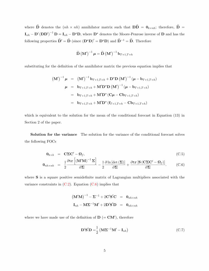
where D denotes the (nh × nh) annihilator matrix such that DD = 0k×nh; therefore, D =
Inh −D′ (DD′)−1
D = Inh −D?D, where D? denotes the Moore-Penrose inverse of D and has the
following properties D′ = D (since (D?D)′ = D?D) and D−1 = D. Therefore
D(M′)−1
µ = D(M′)−1
bT+1,T+h
substituting for the definition of the annihilator matrix the previous equation implies that
(M′)−1
µ =(M′)−1
bT+1,T+h + D?D(M′)−1
(µ− bT+1,T+h)
µ = bT+1,T+h + M′D?D(M′)−1
(µ− bT+1,T+h)
= bT+1,T+h + M′D? (Cµ−CbT+1,T+h)
= bT+1,T+h + M′D? (fT+1,T+h −CbT+1,T+h)
which is equivalent to the solution for the mean of the conditional forecast in Equation (13) in
Section 2 of the paper.
Solution for the variance The solution for the variance of the conditional forecast solves
the following FOCs
0k×k = CΣC′ −Ωf , (C.5)
0nh×nh =1
2
∂tr[(M′M)−1 Σ
]∂Σ
− 1
2
∂ ln [det (Σ)]
∂Σ+∂tr [S (CΣC′ −Ωf )]
∂Σ. (C.6)
where S is a square positive semidefinite matrix of Lagrangian multipliers associated with the
variance constraints in (C.2). Equation (C.6) implies that
(M′M
)−1 −Σ−1 + 2C′S′C = 0nh×nh
Inh −MΣ−1M′ + 2D′S′D = 0nh×nh
where we have made use of the definition of D (= CM′), therefore
D′S′D =
1
2
(MΣ−1M′ − Inh
)(C.7)
5

Equation (C.7) together with Equation (C.5) implies that
D′S′D =
1
2
(MΣ−1M′ − Inh
)S′ =
1
2D?′ (MΣ−1M′ − Inh
)D?
=1
2D?′
[M(C∗ΩfC
∗′)−1M′ − Inh
]D?
=1
2D?′
[MC′Ω−1
f CM′ − Inh
]D?
=1
2D?′
[D′Ω−1
f D′ − Inh
]D?
=1
2(Ω−1
f −D?′D?)
therefore we can solve for the variance under the conditional forecast from Equation (C.7)
MΣ−1M′ = Inh + D′(Ω−1f −D?′D?)D
MΣ−1M′ = D′Ω−1f D + (Inh −D′D?′D?D)
Σ−1 = M−1(D′Ω−1f D + D)
(M′)−1
which implies that
Σ = M′(D′Ω−1f D + D)−1M
= M′(D?ΩfD?′ + D)M
and is equivalent to the solution for the conditional forecast in Equation (14) in Section 2 of the
paper.4
D Details of the algorithm
In this section we develop algorithms to implement structural scenario analysis. Conditional-on-
variables and conditional-on-shocks forecasts can be implemented as special cases of the former.
The algorithms we present can be easily extended to any identification scheme provided that an
4To solve for the variance we have made use of the property that given two square matrices A and B,(A + B)−1 = (A−1 + B−1) if AB−1A = BA−1B (see, e.g., Searle, 1982). The latter conditions in our case
are verified: D′Ω−1f DD−1D′Ω−1
f D =DD?′ΩfD?D = 0nh×nh, since from the definition of the annihilator matrix
DD= 0, and D = D′ and D−1 = D.
6

algorithm is available to draw from the structural parameters. To simplify both the notation and
the exposition, when presenting the algorithm we focus on sign restrictions. Specifically, we extend
the Gibbs sampler algorithm in Waggoner and Zha (1999) to implement the structural scenario
analysis in set and partially identified SVARs.
In particular, we assume that if (A0,A+) satisfy the s sign restrictions, then
F(A0,A+) > 0s×1.
Before describing the algorithm, it should be clear that our objective is to draw from the following
joint posterior
p(yT+1,T+h,A0,A+|yT , IR (A0,A+) ,R (yT+1,T+h,A0,A+)), (D.1)
where IR (A0,A+) = (A0,A+) : F(A0,A+) > 0s×1 are the identification restrictions and
R(yT+1,T+h,A0,A+) = yT+1,T+h : CyT+1,T+h ∼ N(fT+1,T+h, Ωf
) are the restrictions associ-
ated with the structural scenario. Note that R(yT+1,T+h,A0,A+) depends on (A0,A+) because
fT+1,T+h, C, and Ωf depend on (A0,A+).
As explained by Waggoner and Zha (1999), if one wants to take into account identification and
parameter uncertainty, as well as the uncertainty associated with the future path of the shocks
and, possibly, the conditional path of the restricted forecast, drawing the posterior distribution
described by Equation (D.1) becomes a challenging task. It is tempting, in a first step to, draw the
structural parameters from their distribution conditional on yT and the identification restrictions,
and in a second step to draw yT+1,T+h conditional on yT , the restrictions in Equation (15) of the
paper, and the structural parameters, using Equations (13) and (14) of the paper. However, this
procedure ignores the restrictions in Equation (15) when drawing the structural parameters and,
hence, would not lead to a draw from the desired joint posterior described in Equation (D.1). Instead,
to draw from the joint distribution of interest, a Gibbs sampler procedure can be constructed that
iterates between draws from the described conditional distributions of the structural parameters
and yT+1,T+h.5
In this appendix we present a particular implementation of Algorithm 1 that follows Faust
5The algorithm below is an extension of the one developed by Waggoner and Zha (1999), with the key differencebeing that we now need to identify the SVAR.
7

(1998), Uhlig (2005), and Canova and Nicolo (2002), and Rubio-Ramirez et al. (2010) and draw
from a conjugate uniform-normal-inverse-Wishart posterior over the orthogonal reduced-form
parameterization (B,Σ,Q) and transform the draws into the structural parameterization (A0,A+).
Arias et al. (2018) show that this transformation induces a normal-generalized-normal posterior
over the structural parameterization, and highlight the useful properties of using conjugate prior
distributions. On the contrary, Baumeister and Hamilton (2015) prefer to use priors stated directly
over the structural parameterization, (A0,A+). Their argument is that since the implementation
of Arias et al. (2018) amounts to an implicit and informative prior over the objects of interest to
researchers, it is better to define it directly. Baumeister and Hamilton’s (2015) approach has an
advantage when at least some, if not all, the parameters have an economic interpretation, but could
be computationally challenging, especially in large systems. If one wanted to follow that route, our
algorithm could be easily modified to draw directly from (A0,A+).
Algorithm 1. Initialize yT+h,(0) = [yT , y(0)T+1,T+h].
1. Conditioning on yT+h,(i−1) = [yT , y(i−1)T+1,T+h], draw (B(i),Σ(i)) from the posterior distribution
of the reduced-form parameters.
2. Draw Q(i) independently from the uniform distribution over the set of orthogonal matrices.
3. Keep (B(i),Σ(i),Q(i)) if F(f−1h (B(i),Σ(i),Q(i))) > 0s×1, otherwise return to Step 1.
4. Conditioning on (A(i)0 ,A
(i)+ ) = fh(B(i),Σ(i),Q(i)) and yT , draw y
(i)T+1,T+h ∼ N (µy,Σy) using
Equations (10) and (12) of the paper.
5. Return to Step 1 until the required number of draws has been obtained.
The natural initialization of y(0)T+1,T+h can be done at the mean of the unconditional forecast or a
random draw from its posterior. Steps 1 and 2 draw from posterior uniform-normal-inverse-Wishart
over the orthogonal reduced-form parameterization conditional on yT+h,(i−1). Step 3 checks the sign
restrictions, while Step 4 draws y(i)T+1,T+h ∼ N (µy,Σy) using Equations (10) and (12) of the paper.
It is important to notice that because Steps 1 and 2 are conditional on yT+h,(i−1), the restriction in
Equation (15) is taken into account when drawing the structural parameters.
Clearly Steps 1-3 are an accept-reject algorithm to draw from the posterior of (A(i)0 ,A
(i)+ )
conditional on the identification restrictions, as in Rubio-Ramirez et al. (2010), but taking into
account the restrictions on yT+h,(i−1). Step 4 draws y(i)T+1,T+h conditional on (A
(i)0 ,A
(i)+ ) using
8

Equation (15). For the case in which the model is exactly identified, such as in the traditional
recursive ordering using the Cholesky decomposition (see Kilian and Lutkepohl, 2017), the algorithm
is trivially modified by choosing a function h that reflects the restrictions, setting Q = In in Step 2
and skipping Step 3. The algorithm can also be extended to implement the recently proposed
narrative sign restrictions as in Antolin-Diaz and Rubio-Ramirez (2018) and zero restrictions by
the methods described in Arias et al. (2018). In both cases, our algorithm requires an importance-
sampling step to draw from the posterior of (A0,A+), which needs to be done after Step 3. This
approach is known as Gibbs sampling by sampling-importance-resampling as described in Koch
(2007). In particular, the resampling step requires taking multiple draws of the triplet (B,Σ,Q)
by repeating Steps 1-3 above, which are then re-weighted using importance weights as described
in Antolin-Diaz and Rubio-Ramirez (2018) and Arias et al. (2018) respectively. Finally, a random
draw from the reweighted triplets (B,Σ,Q) is selected before proceeding to Step 4.
E Alternative implementation using Kalman filtering
Clarida and Coyle (1984) show that one can implement the Doan et al. (1986) conditional point
forecasts using the Kalman filter. Building on this insight, Banbura et al. (2015) suggest that
state-space methods can also be used to obtain conditional-on-observables forecasts as in Section 2.
We now show that this equivalent algorithm using the Kalman filter can also be applicable to the
structural scenario analysis as well. As we will see, however, the Kalman filter implementation will
be in most cases computationally less efficient than the general, closed-form solutions provided in
the paper. Moreover, it does not easily lend itself to implement more flexible linear restrictions such
as the “Back to the Price Level Target” exercise described in Section 5.
The state-space representation
We begin by outlining the state-space representation that allows the use of the Kalman filter to
compute conditional forecasts. Consider the following state-space form consistent with the model in
Section 2:
z′t = D + z′t−1F + ε′tG (E.1)
y′t = Hz′t (E.2)
9

The state vector z′t = [y′t, . . . ,y′t−p+1, ε
′t] stacks the endogenous variables, their lags, and the
exogenous shocks, where yt is an n× 1 vector of variables at time t, and εt is an n× 1 vector of
structural shocks at time t. The measurement vector y′t = [y′t, ε′t] stacks the endogenous variables
and the exogenous shocks. As we will see below, since the structural shocks are unobserved, the
measurement vector will contain missing observations corresponding to the entries of εt. The system
matrices D, F, G, and H are constructed from the SVAR parameters as shown below:
D =
c
0n·p×1
, F =
Bn·p×n·p
0n·p×n
0n×n·p
0n×n
, G =
h(Σ)Q−1
0n·(p−1)×n
In×n
, H =
In×n
0n×n·p
0n×n·p
In×n
,
where B is known as the companion matrix of the VAR and is defined as
B =
B1 B2 . . . Bp
I 0
0 I. . .
...... I 0
0 . . . . . . 0 I
.
The SVAR representation in Equation 1 of the paper and the state-space representation in
Equations (E.1)-(E.2) described above are equivalent, and both can be used to compute conditional
forecasts. With the model in state-space one can use the simulation smoother (see, e.g., Durbin and
Koopman, 2012) to generate a draw of the state vector y′t, conditional on the observations and the
parameters of the model. Therefore, as outlined by Banbura et al. (2015) for the reduced-form case,
one can treat the future path of conditioning variables as observed, while leaving the future path of
the remaining variables as missing observations.6
The same procedure can be adapted for the case of the structural scenario. Suppose that one
6To allow for missing observations, the standard Kalman filtering recursions must be modified. For this purpose,a number of equivalent solutions have been proposed (see Durbin and Koopman (2012), p. 112, for a textbooktreatment). Here we follow the approach of Mariano and Murasawa (2003) and Camacho and Perez-Quiros (2010),which essentially impose the condition that the Kalman gain associated with the missing observation is mechanicallyzero. This implies that the Kalman filter ”skips” missing observations, effectively marginalizing the likelihood withrespect to the missing observations (see Brockwell and Davis (1991), Section 12.3, and Brockwell et al. (1990)).
10

wants to produce forecasts for h time periods into the future. Denote with ? an observation for
which all data entries are missing, denote (yi,t, ?)′ for T + 1 ≤ t ≤ T + h a post-sample observation
in which the value of endogenous variable i is assumed to be known and fixed, the rest being
missing data, and denote (εj,t, ?)′ for T + 1 ≤ t ≤ T + h a post-sample observation in which the
value of structural shocks j is constrained (for instance to reflect its unconditional standard normal
distribution), the observation for other shocks being missing data. All of the cases mentioned
above can be considered special cases of the state-space representation (E.1)-(E.2), in which the
measurement vector is constructed as y′t in the following way:
y′t = [y′t, ∗], for 1 ≤ t ≤ T, (E.3)
y′t = [(yi,t, ∗)′, (∗, θt)′], for T + 1 ≤ t ≤ T + h, (E.4)
where θt denotes the vector of constrained structural shocks and is a 1 × n − 1 draw from the
unconditional distribution of εt, i.e., from an independent standard normal distribution. In other
words, n columns and h rows of missing observations are appended to the data set containing the
endogenous variables, the known future path for variable i for periods T + 1 to T + h is used to
fill the corresponding missing observations, and the missing observations for the structural shocks
other than the shock of interest are filled in with draws from their unconditional distribution.7 In
Step 4 of Algorithm 1, one can then draw y(i)T+1,T+h using the Kalman smoother, as opposed to
a multivariate Gaussian distribution with mean and variance given by Equations (10)-(12) of the
paper. These two procedures produce identical results.
Computational efficiency
Since the Kalman filtering-based procedure provides results identical to those of the algorithm
outlined in the paper, we now assess which of the two methods is more computationally efficient.
Equations (10)-(12) of the paper involve operations of high dimensional matrix objects which
modern computing langues are well suited to compute efficiently, whereas the procedure based on
the Kalman filter works recursively leading to a higher computational burden.
Table E.1 investigates which of the two procedures is more efficient numerically for different
7If one is interested in computing only point forecasts, filling them with zeros, the unconditional mean, isappropriate.
11

Table E.1: Computational efficiency of conditional forecast methods
p = 1 p = 6 p = 12 p = 24Horizon Baseline KF Baseline KF Baseline KF Baseline KF
n=3
h=1 0.49 27.37 0.5 34.68 0.52 51.77 0.56 88.15h=6 0.8 28.09 1.12 35.32 2.25 49.02 2.11 90.35h=12 1.29 28.48 3.1 36.17 5.53 50.24 5.42 95.68h=24 2.78 29.76 5.06 37.92 8.89 52.72 20.28 98.19h=60 12.37 33.61 18.51 43.38 31.35 59.67 69.64 113.28
n=7
h=1 0.53 35.57 0.55 66.81 0.51 141.74 0.61 368.3h=6 1.42 36.21 2.47 67.34 3.07 139.76 3.03 375.16h=12 2.81 37.17 4 69.25 5.43 147.83 7.79 386.21h=24 9.16 38.68 11.81 72.16 16.72 148.68 28.05 403.88h=60 77.07 43.67 83.9 84.62 102.7 174.42 150.89 458.84
n=11
h=1 0.58 34.04 0.61 93.49 0.55 200.4 0.68 697.13h=6 2.12 35.06 2.58 91.7 3 209.97 3.82 738.55h=12 5.61 36.02 7.6 94.64 9.97 218.71 11.62 751.22h=24 25.31 38.38 25.36 99.79 31.52 231.55 48.95 821.48h=60 210.07 44.63 216.67 126.62 247.11 277.71 308.01 964.74
n=27
h=1 0.9 131.52 0.65 579.93 1.28 2241.43 0.99 12193.3h=6 8.98 130.98 9.17 622.57 10.34 2314.67 12.88 12335.05h=12 35.94 135.65 40.92 599.76 45.23 2351.54 52.18 12644.66h=24 224.8 135.44 224.38 625.57 248.64 2461.27 285.89 13288.57h=60 6301.38 158.01 3874.75 732.05 3980.7 2857.22 4089.79 15290.47
Note: The numbers denote the average time, in seconds (over 100 iterations), taken to calculate 1000 draws ofconditional forecasts. n denotes the number of variables in the VAR, h denotes the forecast horizon and p denotes thenumber of lags in the VAR. The time of the fastest algorithm in each case is marked in boldface. These computationswere performed in Matlab 2015a on an HP Z230 SFF workstation with an Intel Core i7-4770 CPU 3.40GHz processorand 7.74GB of usable RAM.
hypothetical problem settings.8 The baseline implementation of Algorithm 1 is faster in the majority
of cases, with the gains particularly large whenever the number of variables n or lags p is large.
Only whenever h increases a lot relative to the number of variables and lags is small, drawing the
conditional forecast using the Kalman smoother is more efficient.
F Details on the applications
Application 1: Monetary policy alternatives
Data
We work with the data set of Smets and Wouters (2007), which contains seven key US macroeconomic
time series at the quarterly frequency: real output, consumption, investment, wages and hours
8We use deJong’s (1988) implementation of the Kalman filter, as Banbura et al. (2015) show that this implemen-tation is computationally faster than alternative implementations.
12

worked per capita, inflation as measured by the GDP deflator and the federal funds rate.9 Their
data set starts in Q1 1966, and we update it through Q4 2019. For the comparison with the DSGE
model in Section 5, we use the original dataset in Smets and Wouters, downloaded from the AER
website. We verified that the original dataset corresponds to the vintage available in March 2005.
We make one modification to the dataset, which is to substitute the GDP deflator for the PCE
deflator excluding food and energy as an indicator for inflation. We use the data for the March
2005 vintage. The motivation for this change is to be consistent with the fact that the Federal
Reserve’s inflation objective is stated in terms of the PCE deflator, and in particular many of its
communications and internal documents refer to the less volatile ex-food and energy measure as an
more reliable indicator of future inflation tendencies. Over the sample considered, the core PCE
and the overal GDP deflator are 93% correlated.
For the applications updated through 2019, we udpate the dataset using data from Haver
Analytics and using the corresponding tickers:
1. Gross Domestic Product (GDV@USECON)
2. Gross Domestic Product - Implicit Price Deflator (JGDP@USECON)
3. Core PCE Deflator (LXEHL@USECON)
4. Personal Consumption Expenditures, Non-Durable Goods and Services (CS@USECON +
CN@USECON)
5. Fixed Private Investment + Consumer Durables (F@USECON + CD@USECON)
6. Total Economy Hours Worked (LXEHL@USECON)
7. Compensation of Employees (YCOMP@USECON)
8. Civilian Non-Institutional Population (LNN@USECON)
9. Federal Funds Rate (FFED@USECON)
Output, Consumption and Investment are divided by the GDP deflator and by population to obtain
real, per-capita series. Hours are divided by population. Compensation is divided by hours worked
and the GDP deflator to obtain real compensation per hour. To construct the measure of expect
9See the data appendix in Smets and Wouters (2007) for exact definitions of the variables.
13

interest rates we use series from the Philadelphia Fed Survey of Professional Forecasters 3 month
T-bill expecations:
1. Current Quarter (ASAFC3T@SURVEYS)
2. 1 Quarter Ahead (ASAF13T@SURVEYS)
3. 2 Quarter Ahead (ASAF23T@SURVEYS)
4. 3 Quarter Ahead (ASAF33T@SURVEYS)
5. 4 Quarter Ahead (ASAF43T@SURVEYS)
Then, the variable
St,h ≡ ESPFt [it+h]− ESPFt−1 [it+h] (F.1)
for h = 0, . . . , 3 measures the surprise to expectations, i.e., the change in the information set, from
t− 1 to t. Campbell et al. (2012) point out that surprises across horizons h exhibit a strong factor
structure, so we take the average across horizons, St ≡ 1/4∑3
h=0 St,h as a measure of the surprises
to the average expected interest rate for the next year.
Estimation settings
We estimate a VAR with p = 4 lags using Bayesian methods and an informative “Minnesota” prior
(Doan et al., 1986; Sims, 1993) over the reduced-form parameters. Also see Karlsson (2013) In order
to deal with the absence of data for the survey in the early part of the sample, we need to add an
additional step to Algorithm 1. We cast the model in state-space and, conditional on the previous
draw of the reduced-form parameters, we draw the missing observations using a simulation smoother
(e.g., Durbin and Koopman, 2012)
Application 2: Stress-testing
Data
In this section we report the definition and Haver mnemonics for the data used in Application 2,
which are appended to the dataset used in Application 1:
• 3-month Treasury bill rate (FTBS3@USECON)
14

• unemployment rate (LR@USECON)
• 10-year yield (FCM10@USECON)
• S&P 500 index (SP500@USECON)
• house price index (USRSNHPM@USECON)
• oil price deflated by the core PCE deflator (PZTEXP@USECON/JCXFE@USECON)
• credit spread is the BAA credit spread minus the treasury long-term composite yield (FBAA@USECON-
FLTG@USECON)
• TED spread (C111FRED@OECDMEI - FTBS3@USECON)
• ROE for all FDIC Insured Institutions (USARQ@FDIC).
The data are quarterly from 1966 to 2019.
Estimation settings
The VAR is estimated with gour lags and the Minnesota prior implemented using dummy observations
(see Del Negro (2011) for details) over the reduced-form parameters.
G Anticipated Policy Shocks in the Smets-Wouters model
In the empirical section we compare the results from the VAR to the ones from a modified version
of the Smets and Wouters (SW) model. In this appendix we describe the main modifications of the
model and explain the use we make of it, in particular to inform us on the restrictions to impose for
the identification of the anticipated monetary policy shock and on the feasibility of the identification
of the structural shocks from the VAR.
The only modification of the model is the introduction of anticipated monetary policy shocks.
In particular, modify the policy rule in the original model and introduce news shocks as follows
rt = ρrt−1 + (1− ρ)[rππt + rY (yt − ypt )] + ρ∆y[(yt − ypt )− (yt−1 − ypt−1)] + εrt +3∑j=0
vrt−j,j (G.1)
where vrt−j,j is an anticipated monetary policy shock, which corresponds to deviations from the
normal conduct of policy revealed at time t − j yet affecting the interest rate with a delay of j
15

Figure G.1: Federal Fund Surprises
1982 1987 1993 1998 2004 2009 2015-2.5
-2
-1.5
-1
-0.5
0
0.5
1
1.5
2
2.5
h=0h=1h=2h=3
1982 1987 1993 1998 2004 2009 2015-2.5
-2
-1.5
-1
-0.5
0
0.5
1
1.5
Cross-sectional AverageFirst Principal Component
Note. The left chart reports St,h ≡ ESPFt [it+h]−ESPF
t−1 [it+h], for h = 0, . . . , 3. The right panel of the figurecontrasts the cross sectional average of the surprises with their first principal component.
quarters. In order to capture that idea that forward guidance announcements affect the path of the
interest rate over multiple quarters, we assume that news shocks follow a simple MA(4) structure:
vrt−j,j = ηrt−j j = 0, . . . , 3 (G.2)
The way we enter anticipated monetary policy shocks into the model is in line with Campbell et
al. (2012). The simplifying assumption of a single factor structure in equation G.2 reflects the
observations that revisions in interest rate forecast at different quarters display a strong comovement
and roughly equal volatility, as highlighted in Figure G.1. Therefore the key difference between a
standard (unanticipated) monetary policy shock and a ’forward’ guidance shock is that the latter is
expected to affect the path of the interest rate for prolonged periods of time. In order to stay as
close possible to the original SW model we assume that the law of motion of ηrt follows an AR(1)
and fix the parameters of this to be the same as the one of the unanticipated monetary policy shock.
The first question that we ask from the model is whether a seven variables VAR – featuring the
original variables in the SW model – would able to recover an anticipated monetary policy shock, i.e.
more specifically whether the VAR is informationally sufficient or fundamental. Fernandez-Villaverde
et al. (2007) put forward a simple metric, the ‘poor man invertibility condition’ (PMIC), which we
can check on the implied VAR solution in the theoretical model. Fixing the parameters estimates
to the modal estimate in SW, the PMIC shows that a 7 variables VAR is not fundamental in the
structural shocks. However, expanding the model so as to include the average forecast revisions in
16

the short term interest rate suggests that a VAR augmented with a surprise variable calculated as
described in the text satisfies the invertibility requirement and is therefore informationally sufficient.
This is computed in line with the definition given in Section 5 of the paper (equation (F.1) above)
and with expectations computed under the assumption of rationality. However, we do not need the
survey expectations to be fully rational in order for the VAR to be fundamental and identification
to work.
We also use the model to derive plausible restrictions for the identification of the SVAR.
Simulations from the model suggest that an anticipated monetary policy shock is associated with
a pattern of signs of the IRFs which is consistent with the one of a traditional monetary policy
shock. An anticipated monetary policy shock is also associated with a movement in the interest rate
surprise variable, St that goes in the same direction than the shock. When comparing the impact
of an unanticipated and an anticipated MP shock it is clear that, for a shock normalized to have
the same initial impact on the short term interest rate, the anticipated monetary policy shocks are
associated with larger average revisions in St than in the unanticipated case.10 Figure G.2 compares
the impulse response function of the SVAR and the SW model for a monetary policy (MP) shock
and the anticipated monetary policy (AMP) shock. The SVAR model is associated with a more
persistent effect of both shocks, but otherwise the IRFs are remarkably similar despite the fact that
the shocks in the SVAR are estimated imposing only a limited number of identification restrictions.
10Intuitively, with policy rule (G.1) a shock to ηrt that rises the interest rate by 25bp increases the surprise variableSt roughly 4 times more than a shock to εrt .
17

Figure G.2: Impulse Responses: VAR vs. SW model
GDP to MP
0 5 10 15 20
-4
-2
0 GDP to AMP
0 5 10 15 20
-10
-5
0
CONS to MP
0 5 10 15 20
-3
-2
-1
0 CONS to AMP
0 5 10 15 20
-10
-5
0
INV to MP
0 5 10 15 20-20
-10
0 INV to AMP
0 5 10 15 20
-30
-20
-10
0
WAGE to MP
0 5 10 15 20
-4
-2
0 WAGE to AMP
0 5 10 15 20-15
-10
-5
0
HOURS to MP
0 5 10 15 20-4
-2
0
HOURS to AMP
0 5 10 15 20-10
-5
0
INFL to MP
0 5 10 15 20
-0.5
0 INFL to AMP
0 5 10 15 20-2
-1
0
FEDFUNDS to MP
0 5 10 15 20
0
0.5
1 FEDFUNDS to AMP
0 5 10 15 20
-1
0
1
SURPAVG to MP
0 5 10 15 20-0.2
0
0.2
0.4
SURPAVG to AMP
0 5 10 15 20
0
0.5
1
Note. Impulse responses to a monetary policy shock (left column) and an anticipated monetary policyshock (right column). Red continuous line corresponds to the IRFs from the SW model, whereas bluedotted lines corresponds to the IRFs from the SVAR, the blue shaded area represents the 68% (point-wise)HPD credible sets for the IRFs.
18

H Comparison with Fed Staff Estimates in May 2006
In this section we compare results using our SVAR with internal exercises conducted by the Fed
Staff using the FRB/US model and available as part of declassified historical materials. We have
taken the results of the exercises published in the Bluebook dated May 5, 2006.11 We re-estimate
the model using the vintage of data available at that time. We also appended the unemployment
rate to the dataset used in the VAR in order to obtain a conditional forecast of this variable as well
that we can compare with the Fed staff estimates.
In this meeting, the FOMC was presented with two alternatives. The first is the Greenbook
baseline in which the fed funds rate is raised to 5% and then lowered below 4.75%. To shed
light on the implications of ending the process of policy firming, a second simulation considers
a policy trajectory in which the federal funds rate is held constant at its current level through
2010 rather than being raised to 5%. Figure H.1 shows the comparison of the two scenarios, with
the corresponding results published by the Fed staff. In the description of the Bluebook, the staff
mentions that “ monetary policy adjusts to hold core PCE inflation at about 2 percent” so we
condition on inflation being at 2% in expectation at the end of the horizon. They also state the
“assumption that this policy path is fully anticipated by financial market participants” which in our
framework is operationalized as allowing both anticipated and unanticipated shocks to deviate from
their unconditional distribution, and “the absence of any significant supply shocks or changes in
expectations”, which in our setting we model as all non-policy shocks to be at their unconditional
distribution.
It is interesting to note that while the median of the SVAR result is quite close to the FRB/US
result for the unemployment rate, inflation is projected to be higher with the SVAR than with the
FRB/US in both scenarios. This is a result of the federal funds rate staying persistently below the
SVAR unconditional forecast throughout the forecast horizon, reflecting a sequence of monetary
policy shocks which also drive up inflation above the 2% target. One interpretation of our results is
that the SVAR would have suggested that the Fed staff forecasts are too optimistic on the inflation
front, and that further interest rate increases would be required to stabilize inflation. In the event,
this is what happened, with the FOMC ultimately increasing the federal funds rate to 5.25% and
inflation stabilizing around 2%. The mode of the KL is 0.80 for both exercises. The reason the
11See https://www.federalreserve.gov/monetarypolicy/files/FOMC20060510bluebook20060505.pdf (Chart5).
19

scenario is deemed to be a relatively implausible one is because it embodies a highly persistent
deviation from the unconditional scenario at the end of the forecast horizon.
20

Figure H.1: FOMC Monetary Policy Alternatives: May 2006
(a) Baseline
Unemployment Rate
2002 2004 2006 2008 20103
3.5
4
4.5
5
5.5
6
6.5
7
7.5
8
%
Core PCE inflation
2002 2004 2006 2008 20100
0.5
1
1.5
2
2.5
3
3.5
4
4.5
5
% p
.a. (
4-qu
arte
r av
erag
e)
Federal Funds Rate
2002 2004 2006 2008 20100
1
2
3
4
5
6
7
8
% p
.a.
(b) Lower near-term funds rate
Unemployment Rate
2002 2004 2006 2008 20103
3.5
4
4.5
5
5.5
6
6.5
7
7.5
8
%
Core PCE inflation
2002 2004 2006 2008 20100
0.5
1
1.5
2
2.5
3
3.5
4
4.5
5
% p
.a. (
4-qu
arte
r av
erag
e)
Federal Funds Rate
2002 2004 2006 2008 20100
1
2
3
4
5
6
7
8%
p.a
.
Note: For each panel, the solid black lines represent actual data. In the third column, the solid red line and associatedshaded areas are the median, 40 and 68% pointwise credible sets around the conditioning assumptions for the federalfunds rate. In the first and second panel, the solid blue line and associated shaded areas are the median, 40 and68% pointwise credible sets around the forecasts of the other variables given by the SVAR. The dotted gray linesrepresent the median unconditional forecast from the SVAR. The broken black lines represent instead the results ofthe simulations from the FRB/US model as reported in the Fed Bluebook in May 2006.
21

I Narrative Evidence of Fed forward guidance
In this appendix we provide evidence in support of the narrative identification restrictions used to
complement the sign restrictions in the paper. In particular we report extract of FOMC documents
in the periods 2003-2004 and 2011-2012 that justify our choices.
FOMC communication and forward guidance: 2003-2004
In order to enhance the communications with the public, since January 2000 the FOMC started to
issue a brief public statement after every FOMC meeting. The FOMC’s immediate announcement
has contained a summary rationale for its policy decision and encapsulate the Committee’s view of
future developments. On some occasions, the announcement has directly hinted at the likelihood of
changes in policy. The statement has been kept brief, partly to improve the predictability of the
market reaction. Unsurprisingly, from the very beginning the FOMC statements have attracted
considerable attention from the media and the markets, with the language closely watched with
regard both to the current decision and to clues about future policy settings. In particular, special
attention is paid to any changes in wording since the last statement. The first statements used
the “balance of risk” assessment as a way of conveying the most likely ‘tilt’ in future policy. This
practice had however at time come under intense scrutiny. In fact, “the meaning of the balance-of
risks sentence is somewhat vague, giving rise to differences of opinion even among FOMC members
and possibly leading to difficulties among outsiders in understanding its subtleties.” (p. 191).12
Governor Bernanke highlights the importance of giving more precise guidance on the policy
stance. In particular, for the August 12, 2003 meeting transcript Bernanke says (page 131):
“Our discussion yesterday and our experience of the past year have shown that effective commu-
nication is a big part of successful monetary policymaking. [. . . ] We can communicate to financial
markets how we expect to manage short-term interest rates in the future. If we then follow through
on our commitments, the power of our interest rate instrument is multiplied many times over. [. . . ]
Nevertheless, communication that is entirely qualitative in nature also risks misunderstanding. [. . . ]
In an environment of low inflation and low interest rates, we need to seek ever greater clarity of
communication to the markets and to the public.” In mid-2003 the FOMC starts to give a more
explicit reference to the future monetary policy path.
12See https://www.federalreserve.gov/monetarypolicy/files/FOMC20030624memo01.pdf
22

The September 14, 2003 FOMC meeting is dedicated to the discussion of the FOMC communi-
cation policy and procedure around it. In this meeting Gov. Bernanke makes the point that explicit
communication in the FOMC statement should be used to convey information about the policy that
is not only about the FOMC view on the economy: “[. . . ] we shouldn’t be giving unconditional
information about our interest rate setting. We should be trying to guide the market by providing
conditional forecasts about which direction our policy may be going in light of our objectives, our
views, or the nature of our rule.”
August 12, 2003 FOMC Meeting: Negative anticipated monetary policy shock
FOMC Statement The Committee perceives that the upside and downside risks to the attainment
of sustainable growth for the next few quarters are roughly equal. In contrast, the probability, though
minor, of an unwelcome fall in inflation exceeds that of a rise in inflation from its already low level.
The Committee judges that, on balance, the risk of inflation becoming undesirably low is likely to be
the predominant concern for the foreseeable future. In these circumstances, the Committee believes
that policy accommodation can be maintained for a considerable period.
Minutes While the Committee could not commit itself to a particular policy course over
time, many of the members referred to the likelihood that the Committee would want to keep policy
accommodative for a longer period than had been the practice in past periods of accelerating economic
activity. Reasons for such an approach to policy stemmed from the need to encourage progress toward
closing the economy’s currently wide output gap and, with inflation already near the low end of
what some members regarded as an acceptable range, to resist significant further disinflation. [. . . ]
At the same time, maintaining an accommodative policy stance was seen as involving little risk
of inducing rising inflation so long as high levels of excess capacity and very competitive markets
continued to characterize economic conditions.
Additional support for the choice of this data as an example of forward guidance comes from
the Transcripts of the 28 Jan 2004 FOMC meeting. For instance, in his prepared remarks the
FOMC secretary Reinhart states: “At times over the past six months, members have chaffed at the
constraint imposed by the commitment to keep policy accommodative for a considerable period. But
by being explicit to the public about this self-imposed constraint, you did help limit the tendency of
market participants to build in unhelpfully aggressive expectations of policy firming, thereby keeping
financial conditions accommodative at a time when you might have been concerned about the efficacy
23

of alternative monetary policy actions. In the event, the expansion of aggregate demand did not
falter, and there was no need to dig deeper into the toolkit of policymaking.”
In the same meeting Gov. Kohn makes the following remark: “The “considerable period” phrase
was inserted as a form of unconventional policy when we were concerned about deflation and the
lower nominal bound.”
Jan. 28, 2004 FOMC Meeting: Negative anticipated monetary policy shock
The Committee perceives that the upside and downside risks to the attainment of sustainable growth
for the next few quarters are roughly equal. The probability of an unwelcome fall in inflation has
diminished in recent months and now appears almost equal to that of a rise in inflation. With
inflation quite low and resource use slack, the Committee believes that it can be patient in removing
its policy accommodation.
Minutes “With regard to the wording of the Committee’s press statement to be released shortly
after the meeting, members discussed at some length the desirability of retaining a reference from
earlier statements to the prospect that an accommodative policy could be maintained “for a considerable
period.” [...] All the members agreed that a change in wording was desirable, not to signal a policy
tightening move in the near term, but rather to increase the Committee’s flexibility to take such an
action when it was deemed to be desirable and to underline that any such decision would be made on
the basis of evolving economic conditions. [...] A number of members commented that expectations
of sustained policy accommodation appeared to have contributed to valuations in financial markets
that left little room for downside risks, and the change in wording might prompt those markets to
adjust more appropriately to changing economic circumstances in the future. ”
A reading of the transcripts of the discussion in the FOMC highlights that the change in
wording in the statement it transpires that the statement is meant to highlight the FOMC different
assessment of state of the economy and therefore to align market expectations to the one of the
FOMC, which sees a future tightening of policy more likely than what the markets were predicting.
Transcripts “ That there remains considerable mass on the possibility of earlier tightening
embedded in financial market prices implies that there is a potential for the rally to be extended as
expectations correct more to the Greenbook baseline. Why market participants might still expect
earlier and more significant firming is evident in the bottom right panel: A survey of economists at
eight dealers indicates that their outlook for inflation is decidedly less subdued than the staff’s, even
24
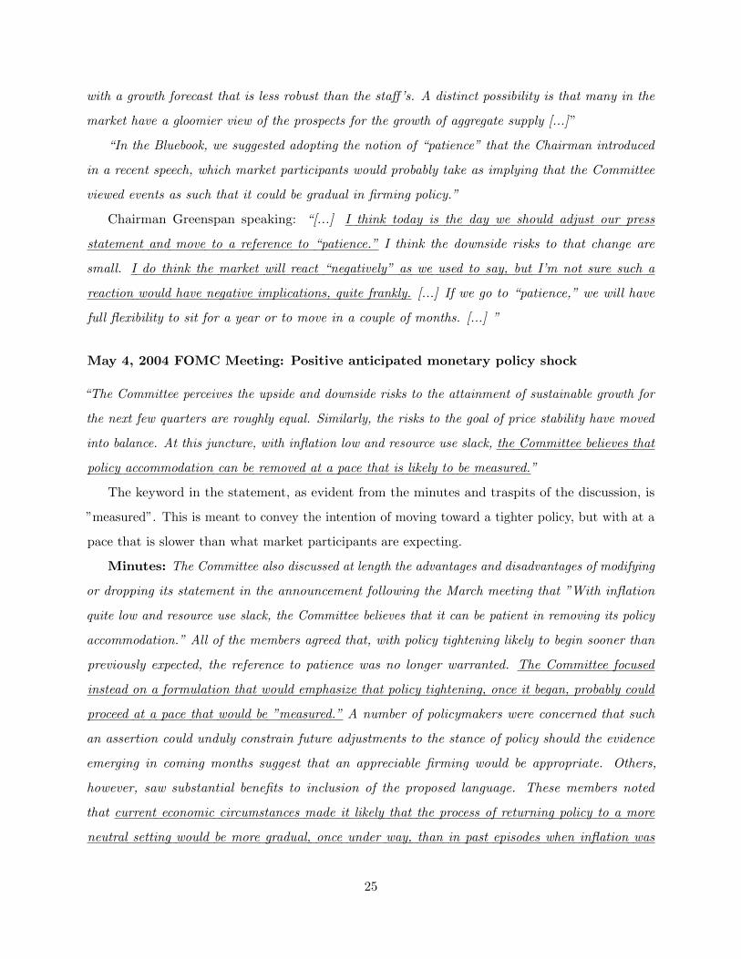
with a growth forecast that is less robust than the staff’s. A distinct possibility is that many in the
market have a gloomier view of the prospects for the growth of aggregate supply [...]”
“In the Bluebook, we suggested adopting the notion of “patience” that the Chairman introduced
in a recent speech, which market participants would probably take as implying that the Committee
viewed events as such that it could be gradual in firming policy.”
Chairman Greenspan speaking: “[...] I think today is the day we should adjust our press
statement and move to a reference to “patience.” I think the downside risks to that change are
small. I do think the market will react “negatively” as we used to say, but I’m not sure such a
reaction would have negative implications, quite frankly. [...] If we go to “patience,” we will have
full flexibility to sit for a year or to move in a couple of months. [...] ”
May 4, 2004 FOMC Meeting: Positive anticipated monetary policy shock
“The Committee perceives the upside and downside risks to the attainment of sustainable growth for
the next few quarters are roughly equal. Similarly, the risks to the goal of price stability have moved
into balance. At this juncture, with inflation low and resource use slack, the Committee believes that
policy accommodation can be removed at a pace that is likely to be measured.”
The keyword in the statement, as evident from the minutes and traspits of the discussion, is
”measured”. This is meant to convey the intention of moving toward a tighter policy, but with at a
pace that is slower than what market participants are expecting.
Minutes: The Committee also discussed at length the advantages and disadvantages of modifying
or dropping its statement in the announcement following the March meeting that ”With inflation
quite low and resource use slack, the Committee believes that it can be patient in removing its policy
accommodation.” All of the members agreed that, with policy tightening likely to begin sooner than
previously expected, the reference to patience was no longer warranted. The Committee focused
instead on a formulation that would emphasize that policy tightening, once it began, probably could
proceed at a pace that would be ”measured.” A number of policymakers were concerned that such
an assertion could unduly constrain future adjustments to the stance of policy should the evidence
emerging in coming months suggest that an appreciable firming would be appropriate. Others,
however, saw substantial benefits to inclusion of the proposed language. These members noted
that current economic circumstances made it likely that the process of returning policy to a more
neutral setting would be more gradual, once under way, than in past episodes when inflation was
25

well above levels consistent with price stability. In addition, some policymakers observed that the
timing and magnitude of future policy adjustments would ultimately be determined by the Committee’s
interpretation of the incoming data on the economy and prices rather than by its current expectation
of those developments. On balance, all the members agreed that they could accept an indication
in the statement that ”. . . policy accommodation can be removed at a pace that is likely to be
measured.”
Transcripts In the Bluebook, we offered modified language that the “Committee believed that
policy accommodation can likely be removed at a measured pace” to emphasize that you see yourselves
entering a tightening phase but one that likely will not be as aggressive as in prior episodes. That
emphasis seemed important because, as in the table at the bottom left, market participants currently
anticipate about 200 basis points of firming in the next year. That is probably influenced by the
experience of the three prior tightening phases, in which the funds rate moved an average of 2 2/3
percentage points higher within the first year. But with inflation lower now than in those prior
episodes, you may see less need at this juncture for such firming, perhaps viewing as more likely
something on the order of the 100 basis point increase assumed by the staff. In the Greenbook, the
gradual realization by investors that you will not need to tighten as sharply as they now believe
imparts an accommodative offset to your policy firming. Without that offset, you may be concerned
that the swing of both monetary and fiscal policies toward more restraint may slow the growth of
spending next year even more than is built into the Greenbook.
FOMC Forward Guidance: 2011 - 2012
August 9, 2011 FOMC Meeting: Negative anticipated monetary policy shock
Statement. “The Committee currently anticipates that economic conditions–including low rates of
resource utilization and a subdued outlook for inflation over the medium run–are likely to warrant
exceptionally low levels for the federal funds rate at least through mid-2013. [. . . ] The Committee
discussed the range of policy tools available to promote a stronger economic recovery in a context of
price stability. It will continue to assess the economic outlook in light of incoming information and
is prepared to employ these tools as appropriate.”
Minutes. “In the discussion of monetary policy for the period ahead, most members agreed
that the economic outlook had deteriorated by enough to warrant a Committee response at this
meeting. While all felt that monetary policy could not completely address the various strains on the
26

economy, most members thought that it could contribute importantly to better outcomes in terms of
the Committee’s dual mandate of maximum employment and price stability. In particular, some
members expressed the view that additional accommodation was warranted because they expected the
unemployment rate to remain well above, and inflation to be at or below, levels consistent with the
Committee’s mandate.”
From the transcripts it is clear that the statement chosen, over the various alternative considered
reflects the intention of providing additional stimulus to the economy. This for instance transpires by
the Secretary of the FOMC, Mr. English, description of the rationale for adopting the statement that
was eventually released. Specifically, he mentions “With the incoming data over the intermeeting
period suggesting an even weaker outlook for economic activity, some participants may feel that
it is now appropriate to provide additional accommodation, as in alternative A. [. . . ] Regarding
monetary policy, alternative A would include two steps to provide additional accommodation. First,
paragraph 3 would provide more-explicit forward guidance about the expected path for the federal
funds rate by specifying that exceptionally low levels were likely “at least through mid2013.” Second,
[. . . ] Although expectations may have moved in recent days, market participants would probably still
be surprised by the adoption of alternative A. Interest rates and the foreign exchange value of the
dollar would likely fall, and stock prices would probably increase.”
January 24-25, 2012 FOMC Meeting: Negative anticipated monetary policy shock
Statement. “To support a stronger economic recovery and to help ensure that inflation, over
time, is at levels consistent with the dual mandate, the Committee expects to maintain a highly
accommodative stance for monetary policy. In particular, the Committee decided today to keep the
target range for the federal funds rate at 0 to 1/4 percent and currently anticipates that economic
conditions–including low rates of resource utilization and a subdued outlook for inflation over the
medium run–are likely to warrant exceptionally low levels for the federal funds rate at least through
late 2014.”
Minutes. “With respect to the statement to be released following the meeting, members agreed
that only relatively small modifications to the first two paragraphs were needed to reflect the incoming
information and the modest changes to the economic outlook implied by the recent data. In light
of the economic outlook, almost all members agreed to indicate that the Committee expects to
maintain a highly accommodative stance for monetary policy and currently anticipates that economic
27

conditions–including low rates of resource utilization and a subdued outlook for inflation over the
medium run–are likely to warrant exceptionally low levels for the federal funds rate at least through
late 2014, longer than had been indicated in recent FOMC statements. In particular, several members
said they anticipated that unemployment would still be well above their estimates of its longer-term
normal rate, and inflation would be at or below the Committee’s longer-run objective, in late 2014.
It was noted that extending the horizon of the Committee’s forward guidance would help provide
more accommodative financial conditions by shifting downward investors’ expectations regarding the
future path of the target federal funds rate. Some members underscored the conditional nature of the
Committee’s forward guidance and noted that it would be subject to revision in response to significant
changes in the economic outlook.”
From the transcripts it is clear that the statement chosen, over the various alternative considered
reflects the intention of providing additional stimulus to the economy. This for instance transpires by
the Secretary of the FOMC, Mr. English, description of the rationale for adopting the statement that
was eventually released. Specifically, he mentions “However, your SEP submissions suggest that you
see only modest economic growth over coming quarters, with the unemployment rate declining even
more slowly than you anticipated at the time of the November SEP. [...] With regard to inflation,
the SEP results suggest that most of you see inflation as likely to be subdued. Against this backdrop,
you may wish to ease financial conditions a bit further by providing forward guidance that pushes
out the expected date of the liftoff of the federal funds rate. You may also think it helpful to provide
clear guidance regarding the economic conditions that would warrant retaining the current very low
level of the federal funds rate. [...] Market participants see significant odds that the Committee
will raise the funds rate by the middle of 2014, and so specifying a date of “at least through late
2014” would likely push out somewhat expectations for the date of the first increase in the funds
rate. Longer-term interest rates would likely decline a little, equity prices could rise some, and the
foreign exchange value of the dollar might soften. ”
September 12-13, 2012 FOMC Meeting: Negative anticipated monetary policy shock
Statement. “ The Committee is concerned that, without further policy accommodation, economic
growth might not be strong enough to generate sustained improvement in labor market conditions.
Furthermore, strains in global financial markets continue to pose significant downside risks to the
economic outlook. The Committee also anticipates that inflation over the medium term likely would
28

run at or below its 2 percent objective.[...] To support continued progress toward maximum employ-
ment and price stability, the Committee expects that a highly accommodative stance of monetary
policy will remain appropriate for a considerable time after the economic recovery strengthens. In
particular, the Committee also decided today to keep the target range for the federal funds rate at 0
to 1/4 percent and currently anticipates that exceptionally low levels for the federal funds rate are
likely to be warranted at least through mid-2015.”
Minutes. “Members generally judged that without additional policy accommodation, economic
growth might not be strong enough to generate sustained improvement in labor market conditions.
[...] Inflation had been subdued, even though the prices of some key commodities had increased
recently. Members generally continued to anticipate that, with longer-term inflation expectations
stable and given the existing slack in resource utilization, inflation over the medium term would run
at or below the Committee’s longer-run objective of 2 percent.
In their discussion of monetary policy for the period ahead, members generally expressed concerns
about the slow pace of improvement in labor market conditions and all members but one agreed
that the outlook for economic activity and inflation called for additional monetary accommodation.
Members agreed that such accommodation should be provided through both a strengthening of the
forward guidance regarding the federal funds rate and purchases of additional agency MBS at a pace
of $40 billion per month. [...] With regard to the forward guidance, the Committee agreed on an
extension through mid-2015, in conjunction with language in the statement indicating that it expects
that a highly accommodative stance of policy will remain appropriate for a considerable time after
the economic recovery strengthens. That new language was meant to clarify that the maintenance
of a very low federal funds rate over that period did not reflect an expectation that the economy
would remain weak, but rather reflected the Committee’s intention to support a stronger economic
recovery.”
The presentation material for this meeting associated with the alternative monetary policy
options, presents simulations which highlight how the adopted statement was meant to provide
additional stimulus to the economy. In fact, the secretary of the FOMC, Mr. English, states
“The black solid lines in the charts depict the experimental consensus forecast, which is conditioned
on unchanged policy. The red dashed lines show the results of a more accommodative policy, one
that’s consistent with an alternative B that shifts back the date in the forward guidance to mid-2015
and, in addition to $30 billion of MBS purchases a month and completion of the MEP this year,
29

involves buying longer-term securities at a rate of $75 billion a month through the middle of next
year. [...]] So long as the public correctly anticipates that the Committee will follow this policy, the
result is a more rapid economic recovery that takes the unemployment rate to 6.3 percent by the
end of 2015, about 1/2 percentage point lower than in the consensus baseline; the inflation rate
(shown at the bottom right) is a bit higher but remains near your 2 percent longer-run objective. [...]
If, in reviewing the outlook under the unchanged policy, the Committee views the likely outcomes
for employment and inflation as inconsistent with its mandate, it might choose to ease policy by
strengthening the forward guidance in the statement and engaging in additional asset purchases.
Alternative B, on page 5, may offer the Committee an attractive approach to moving strongly in
that direction at this meeting, but without committing now to a large, discrete purchase program. ”
30
J Additional Figures
Figure J.1 analyzes the consequences of the alternative treatments of uncertainty for the density
forecasts for the structural scenario: “What is the likely path of output and inflation, if monetary
policy shocks lower the fed funds rate to 1% and keep it there for two years?”
Figure J.2 shows an alternative scenario for the exercise of returning to the price level target
using only unanticipated shocks. The results indicate that a more volatile interest rate path would
be required to achieve the same objective. The fed funds rate would be cut to 1% by mid-2020 and
then increased to 4.6% in 2023. During that year the probability of negative annual GDP growth
would exceed 50%. Figure J.3 instead shows a scenario in which both anticipated and unanticipated
shocks are used, but the price level returns to the target in 7 years instead of 4 years.
31

Figure J.1: Comparison under Different Treatments of Uncertainty
(a) No Uncertainty (Ωf = 0,Ωg = 0)
GDP per cap. growth
2016 2017 2018 2019 2020 2021-2
-1
0
1
2
3
4
5
6
% p
.a. (
4-qu
arte
r av
erag
e)
Core PCE inflation
2016 2017 2018 2019 2020 2021-2
-1
0
1
2
3
4
5
6
% p
.a. (
4-qu
arte
r av
erag
e)
Federal Funds Rate
2016 2017 2018 2019 2020 20210
1
2
3
4
5
6
% p
.a.
(b) Only Uncertainty about the Non-Driving Shocks (Ωf = 0,Ωg = I)
GDP per cap. growth
2016 2017 2018 2019 2020 2021-2
-1
0
1
2
3
4
5
6
% p
.a. (
4-qu
arte
r av
erag
e)
Core PCE inflation
2016 2017 2018 2019 2020 20210
0.5
1
1.5
2
2.5
3
3.5
4
% p
.a. (
4-qu
arte
r av
erag
e)
Federal Funds Rate
2016 2017 2018 2019 2020 20210
0.5
1
1.5
2
2.5
3
3.5
4
% p
.a.
(c) Full Uncertainty (Ωf = DD′,Ωg = I)
GDP per cap. growth
2016 2017 2018 2019 2020 2021-2
-1
0
1
2
3
4
5
6
% p
.a. (
4-qu
arte
r av
erag
e)
Core PCE inflation
2016 2017 2018 2019 2020 20210
0.5
1
1.5
2
2.5
3
3.5
4
% p
.a. (
4-qu
arte
r av
erag
e)
Federal Funds Rate
2016 2017 2018 2019 2020 20210
0.5
1
1.5
2
2.5
3
3.5
4
% p
.a.
Note: For each panel, the solid black lines represent actual data, the solid red line is the conditioning assumption onthe fed funds rate, the solid blue line is the median forecast for the remaining variables and periods, and the blueshaded areas denote the 40 and 68% pointwise credible sets around the forecasts. The dotted gray lines represent themedian unconditional forecast.
32

Figure J.2: Returning to the Price Level Target: Unanticipated Shocks Only
GDP per cap. growth
2004 2006 2008 2010 2012 2014 2016 2018 2020 2022 2024-6
-4
-2
0
2
4
6
% p
.a. (
4-qu
arte
r av
erag
e)
Core PCE inflation
2004 2006 2008 2010 2012 2014 2016 2018 2020 2022 2024-2
-1
0
1
2
3
4
5
6
% p
.a. (
4-qu
arte
r av
erag
e)
Federal Funds Rate
2004 2006 2008 2010 2012 2014 2016 2018 2020 2022 20240
1
2
3
4
5
6
% p
.a.
Log Price Level
2004 2006 2008 2010 2012 2014 2016 2018 2020 2022 2024
90
100
110
120
130
Inde
x (2
012
Q1
= 1
00)
Note: For each panel, the solid black lines represent actual data. The solid blue lines and associated shaded areasare the median, 40 and 68% pointwise credible sets around the forecasts of the other variables given such that theconstraint that inflation returns to the price level target within a five-year horizon is satisfied. The dotted gray linesrepresent the median unconditional forecast.
33

Figure J.3: Returning to the Price Level Target: Seven Year Horizon
GDP per cap. growth
2004 2006 2008 2010 2012 2014 2016 2018 2020 2022 2024-6
-4
-2
0
2
4
6
% p
.a. (
4-qu
arte
r av
erag
e)
Core PCE inflation
2004 2006 2008 2010 2012 2014 2016 2018 2020 2022 2024-2
-1
0
1
2
3
4
5
6
% p
.a. (
4-qu
arte
r av
erag
e)
Federal Funds Rate
2004 2006 2008 2010 2012 2014 2016 2018 2020 2022 20240
1
2
3
4
5
6
% p
.a.
Log Price Level
2004 2006 2008 2010 2012 2014 2016 2018 2020 2022 2024
90
100
110
120
130
Inde
x (2
012
Q1
= 1
00)
Note: For each panel, the solid black lines represent actual data. The solid blue lines and associated shaded areasare the median, 40 and 68% pointwise credible sets around the forecasts of the other variables given such that theconstraint that inflation returns to the price level target within a seven-year horizon is satisfied. The dotted gray linesrepresent the median unconditional forecast.
34

References
Andersson, M. K., S. Palmqvist, and D. F. Waggoner (2010): “Density Conditional Forecasts in DynamicMultivariate Models,” Sveriges Riksbank Working Paper Series 247, Sveriges Riksbank.
Antolin-Diaz, J. and J. F. Rubio-Ramirez (2018): “Narrative Sign Restrictions for SVARs,” American EconomicReview, 108, 2802–29.
Arias, J. E., J. F. Rubio-Ramirez, and D. F. Waggoner (2018): “Inference Based on SVARs Identified with Signand Zero Restrictions: Theory and Applications,” Econometrica, 86, 685–720.
Banbura, M., D. Giannone, and M. Lenza (2015): “Conditional forecasts and scenario analysis with vectorautoregressions for large cross-sections,” International Journal of Forecasting, 31, 739–756.
Baumeister, C. and J. D. Hamilton (2015): “Sign restrictions, structural vector autoregressions, and useful priorinformation,” Econometrica, 83, 1963–1999.
Ben-israel, A. and T. N. E. Greville (2001): Generalized Inverses: Theory and Applications, PublisherSpringer-Verlag New York, second ed.
Brockwell, P., R. Davis, and H. Salehi (1990): “A state-space approach to transfer-function modeling,” StatisticalInference in Stochastic Processes, 6, 233.
Brockwell, P. J. and R. A. Davis (1991): “Time Series: Theory and Methods,” New York: Springer-Verlag., 66,119–128.
Camacho, M. and G. Perez-Quiros (2010): “Introducing the euro-sting: Short-term indicator of euro area growth,”Journal of Applied Econometrics, 25, 663–694.
Campbell, J. R., C. L. Evans, J. D. Fisher, and A. Justiniano (2012): “Macroeconomic Effects of FederalReserve Forward Guidance,” Brookings Papers on Economic Activity, 43, 1–80.
Canova, F. and G. D. Nicolo (2002): “Monetary disturbances matter for business fluctuations in the G-7,” Journalof Monetary Economics, 49, 1131–1159.
Clarida, R. H. and D. Coyle (1984): “Conditional Projection by Means of Kalman Filtering,” NBER TechnicalWorking Papers 0036, National Bureau of Economic Research, Inc.
deJong, P. (1988): “A cross-validation filter for time series models.” Biometrika, 75, 594–600.
Del Negro, M. (2011): “Bayesian Macroeconometrics,” in The Oxford Handbook of Bayesian Econometrics.
Doan, T., R. B. Litterman, and C. A. Sims (1986): “Forecasting and conditional projection using realistic priordistribution,” Staff Report 93, Federal Reserve Bank of Minneapolis.
Durbin, J. and S. J. Koopman (2012): Time Series Analysis by State Space Methods: Second Edition, OxfordUniversity Press.
Faust, J. (1998): “The robustness of identified VAR conclusions about money,” International Finance DiscussionPapers 610, Board of Governors of the Federal Reserve System (U.S.).
Fernandez-Villaverde, J., J. F. Rubio-Ramırez, T. J. Sargent, and M. W. Watson (2007): “ABCs (and Ds)of Understanding VARs,” American Economic Review, 97, 1021–1026.
Golub, G. H. and C. F. Van Loan (1996): Matrix Computations, The Johns Hopkins University Press, third ed.
Karlsson, S. (2013): “Forecasting with Bayesian vector autoregression,” in Handbook of economic forecasting,Elsevier, vol. 2, 791–897.
Kilian, L. and H. Lutkepohl (2017): Structural Vector Autoregressive Analysis, Cambridge University Press.
35

Koch, K. (2007): “Gibbs sampler by sampling-importance-resampling,” Journal of Geodesy, 81, 581–591.
Mariano, R. S. and Y. Murasawa (2003): “A new coincident index of business cycles based on monthly andquarterly series,” Journal of Applied Econometrics, 18, 427–443.
Penrose, R. (1956): “On best approximate solutions of linear matrix equations,” Mathematical Proceedings of theCambridge Philosophical Society, 52, 17–19.
Rubio-Ramirez, J. F., D. F. Waggoner, and T. Zha (2010): “Structural Vector Autoregressions: Theory ofIdentification and Algorithms for Inference,” Review of Economic Studies, 77, 665–696.
Searle, S. R. (1982): Matrix Algebra Useful for Statistics, John Wiley & Sons.
Sims, C. A. (1993): “A Nine-Variable Probabilistic Macroeconomic Forecasting Model,” in Business Cycles, Indicatorsand Forecasting, National Bureau of Economic Research, Inc, NBER Chapters, 179–212.
Smets, F. and R. Wouters (2007): “Shocks and frictions in US business cycles: A Bayesian DSGE approach,”American economic review, 97, 586–606.
Uhlig, H. (2005): “What are the effects of monetary policy on output? Results from an agnostic identificationprocedure,” Journal of Monetary Economics, 52, 381–419.
Waggoner, D. F. and T. Zha (1999): “Conditional Forecasts in Dynamic Multivariate Models,” Review of Economicsand Statistics, 81, 639–651.
36