structural reforms, animal spirits and monetary policies

European Economic Review 124 (2020) 103395

Contents lists available at ScienceDirect

European Economic Review

journal homepage: www.elsevier.com/locate/euroecorev

Structural reforms, animal spirits, and monetary policies

✩ , ✩✩

Paul De Grauwe

a , ∗, Yuemei Ji b

a London School of Economics, United Kingdom

b University College London, United Kingdom

a r t i c l e i n f o

Article history:

Received 15 July 2019

Accepted 30 January 2020

Available online 7 February 2020

JEL codes:

E1

e12

e32

Keywords:

Animal spirits

Behavioral macroeconomics

Business cycles

Structural reforms

Price flexibility

Labor market

Product market

a b s t r a c t

We use a New Keynesian behavioral macroeconomic model to analyze how structural re-

forms affect the economy. There are two types of structural reforms. The first one increases

price flexibility; the second one increases competition in the labor market and raises po-

tential output. We find that in a rigid economy business cycle movements are dominated

by movements of animal spirits. Increasing price flexibility reduces the power of animal

spirits and the boom bust nature of the business cycle. We study the trade-offs between

output and inflation volatility faced by the central bank. We find that flexibility improves

these trade-offs making it easier for the central bank to stabilize output and inflation.

© 2020 Published by Elsevier B.V.

1. Introduction

As a reaction to the sovereign debt crisis European policy makers intensified calls for structural reforms aiming at mak-

ing economic systems more flexible and more competitive. Countries like Greece, Ireland, and Portugal that were subject

to financial rescue programs in fact were forced to implement structural reforms mainly in the labor market and in pen-

sion systems. Others, like Italy and Spain instituted similar reforms mainly as a result of peer pressure exerted within the

European Union. The underlying view of this approach was that it is crucial for the recovery that the supply side be made

more flexible and more competitive. No doubt the supply side in many countries needs to be reformed. At the same time,

however, aggregate demand matters. Structural reforms imposed on the supply side interact with aggregate demand. It is

this interaction that determines what the short-term and long-term effects of structural reforms will be.

The question of how supply-side reforms interact with aggregate demand and how they impact on the economy has

been analyzed in DSGE-models. Most of the time these reforms are modeled as leading to a decline in the markup between

prices and marginal costs ( ECB 2015 ; Cacciatore et al., 2012, 2016 ; , Eggertson et al., 2014 ; Sajedi, 2017 ). This analysis has

shed new light on how reforms affect the economy in the short and in the long run.

✩ Our research has been made possible by a grant of the ESRC (“Structural Reforms and European Integration”, ES/P0 0 0274/1). ✩✩ We are grateful to two anonymous referees whose comments have contributed to improving the quality of this article.

∗ Corresponding author.

E-mail address: [email protected] (P. De Grauwe).

https://doi.org/10.1016/j.euroecorev.2020.103395

0014-2921/© 2020 Published by Elsevier B.V.


http://www.ScienceDirect.com

http://www.elsevier.com/locate/euroecorev

http://crossmark.crossref.org/dialog/?doi=10.1016/j.euroecorev.2020.103395&domain=pdf

mailto:[email protected]


2 P. De Grauwe and Y. Ji / European Economic Review 124 (2020) 103395

The limitation of the standard DSGE-models is that these models do not have an endogenous business cycle theory. In

these models, business cycles are triggered by exogenous shocks combined with slow adjustments of wages and prices.

There is a need to analyze the effects of structural reforms in models where the business cycle is generated endogenously

interacting with behavioral factors. This is the case in behavioral macroeconomic models (see Farmer and Foley (2009) ,

De Grauwe (2012) , Hommes and Lustenhouwer (2016) , De Grauwe and Ji (2016, 2018) , Agliari et al. (2017) , Hallegatte et al.

(2008) , and Hommes et al. (2019) ; for a survey see Franke and Westerhoff (2017) ).

In this paper, we use a behavioral macroeconomic model based on a New Keynesian framework to analyze the effects of

structural reforms. The model is characterized by the fact that agents experience cognitive limitations preventing them from

having rational expectations. Instead they use simple forecasting rules (heuristics) and evaluate the forecasting performances

of these rules ex-post. This evaluation leads them to switch to the rules that perform best. Thus, it can be said that agents

use a trial-and-error learning mechanism.

This heuristic switching model produces endogenous waves of optimism and pessimism (animal spirits) that drive the

business cycle in a self-fulfilling way, i.e. optimism (pessimism) leads to an increase (decline) in output, and the increase

(decline) in output in term intensifies optimism (pessimism), see De Grauwe (2012) and De Grauwe and Ji (2018) . An im-

portant feature of this dynamics of animal spirits is that the movements of the output gap are characterized by periods of

tranquility alternating in an unpredictable way with periods of intense movements of booms and busts. One of the issues

we will analyze is how structural reforms affect this dynamics of the business cycle.

We will introduce structural reforms in the context of this behavioral model through two channels. The first one is

through the sensitivity of inflation to the output gap in the New Keynesian Philips curve (supply equation). A low sensitivity

of the rate of inflation with respect to the output gap is indicative of price rigidities. For example, if prices are rigid a

decline in the output gap during a recession has a low effect on prices and therefore does not transmit into lower inflation.

Conversely, when prices are flexible, a decline in the output gap is transmitted into a lower rate of inflation.

The second way we will introduce structural reforms is through supply shocks. This is also the way structural reforms

have been modeled in standard DSGE models (see for e.g., Eggertson, et al. (2014) , Cacciatore et al. (2012) , Everaert and

Schule (2006) , Gomes et al. (2013) , and ECB (2015) ). In these microfounded models, structural reforms in labor markets

include relaxing job protection, cuts in unemployment benefits, etc., and in product markets, reductions in barriers to entry

for new firms. These reforms lead to a lowering of mark-ups in the goods and labor markets and move the economy closer to

perfect competition. Therefore, these reforms can be seen as shifting the supply curve to the right, increasing the production

potential of countries. One common feature of these New Keynesian models is their reliance on the assumption that there

are rigidities in nominal prices leading to a relatively flat Philips curve. In such a case, analyzing the right-ward shift of the

supply curve becomes more important.

The main focus of this paper will be the analysis, first, of how structural reforms that increase flexibility affect the nature

of the business cycle, and second, how these structural reforms affect the capacity of the central bank to stabilize inflation

and output.

The paper is organized as follows. Sections 2–4 present the behavioral model, its main characteristics, stability condi-

tion, calibration and empirical verification. Sections 5 and 6 present the results of this model related to structural reforms.

In Section 5 , we compare the features of the output gap and animal spirits under the flexible and the rigid assumption.

Section 6 presents the impulse response results of a positive supply shock. We also compare the major results in the behav-

ioral model with the rational expectations models. Section 7 analyzes the power of output stabilizations and how structural

reforms affect the choices monetary authorities face concerning output stabilizations. Section 8 contains the conclusion.

2. The behavioral model

2.1. Basic model

The model consists of an aggregate demand equation, an aggregate supply equation and a Taylor rule. In Appendix 1 we

provide the microfoundations of this model.

The aggregate demand equation can be expressed in the following way:

y t = a 1 E t y t+1 + ( 1 − a 1 ) y t−1 + a 2 (r t − ˜ E t πt+1

)+ v t (1)

where y t is the output gap in period t, r t is the nominal interest rate, π t is the rate of inflation. The tilde above E refers to the

fact that expectations are not formed rationally. How exactly these expectations are formed will be specified subsequently.

We follow the procedure introduced in New Keynesian DSGE-models of adding a lagged output in the demand equation.

This can be justified by invoking inertia in decision-making. It takes time for agents to adjust to new signals because there

is habit formation or because of institutional constraints (see Dennis (2008) ). For example, contracts cannot be renegotiated

instantaneously.

We assume the aggregate supply equation in (2) . This New Keynesian Philips curve includes a forward looking compo-

nent, ˜ E t πt+1 , and a lagged inflation variable. Inflation π t is sensitive to the output gap y t . The parameter b 2 measures the

extent to which inflation adjusts to changes in the output gap. It is therefore indicative of the degree of price flexibility. In

Appendix 1 , we develop this idea in greater detail and we show how it is related to Calvo pricing.

πt = b 1 E t πt+1 + ( 1 − b 1 ) πt−1 + b 2 y t + ηt . (2)

P. De Grauwe and Y. Ji / European Economic Review 124 (2020) 103395 3

Finally, the Taylor rule describes the behavior of the central bank

r t = ( 1 − c 3 ) [ c 1 ( πt − π ∗) + c 2 y t ] + c 3 r t−1 + u t (3)

where π ∗ is the inflation target, thus the central bank is assumed to raise the interest when the observed inflation rate

increases relative to the announced inflation target. The intensity with which it does this is measured by the coefficient c 1 .

Similarly, when the output gap increases the central bank is assumed to raise the interest rate. The intensity with which it

does this is measured by c 2 . The latter parameter then also tells us something about the ambitions the central bank has to

stabilize output. A central bank that does not care about output stabilization sets c 2 = 0. We say that this central bank applies

strict inflation targeting. The parameter c 1 is important. It has been shown (see Woodford (2003) , chapter 4, or Gali (2008) )

that it must exceed 1 for the model to be stable. This is also sometimes called the “Taylor principle.”

Finally, note that, as is commonly done, the central bank is assumed to smooth the interest rate. This smoothing behavior

is represented by the lagged interest rate r t−1 in Eq. (3) . The long-term equilibrium interest rate is assumed to be zero and

thus it does not appear in the equation.

We have added error terms in each of the three equations. These error terms describe the nature of the different shocks

that can hit the economy. There are demand shocks, v t , supply shocks , ηt , and interest rate shocks, u t . We will generally

assume that these shocks are normally distributed with mean zero and a constant standard deviation.

2.2. Introducing heuristics in forecasting output

We assume that agents lack the cognitive capacities to form rational expectations. The latter indeed require agents to

understand the complexities of the underlying model and to know the frequency distributions of the shocks that will hit

the economy. We take it that the cognitive limitations of agents prevent them from understanding and processing this kind

of information. These cognitive limitations have been confirmed by laboratory experiments and survey data (see Carroll

(2003 ), Branch (2004 ), Pfajfar and Zakelj (2011 , 2014 ), Hommes (2011 )).

There is a large literature on expectations formation (see Evans (2001) ). While some modelers adopt some weaker forms

of rational expectations, namely “eductive learning,” others have developed “adaptive learning” models in macroeconomics.

The latter refer to the possibility that agents learn and update their forecasts. This updating can be done using statistical

methods as in Evans and Honkapopja (2001) or in an evolutionary (trial and error) fashion (see Brock and Hommes (1997) ,

Branch and McGough (2010) , De Grauwe (2012) and Hommes and Lustenhouwer (2019) ).

In this paper, we will use the evolutionary approach to “adaptive learning” approach in which agents use simple rules

(heuristics) to forecast future output gap and inflation. Rationality is introduced by assuming a willingness to learn from

mistakes and therefore a willingness to switch between different heuristics. In making these choices we follow the road

taken by an increasing number of macroeconomists, which have developed “agent-based models” and “behavioral macroe-

conomic models” (see for example Tesfatsion (2001) , Colander et al. (2008) , Farmer and Foley (2009) , Delli Gatti et al. (2005) ,

Westerhoff and Franke (2018) , De Grauwe (2012) , Hommes and Lustenhouwer (2019) ).

The way we proceed is as follows. We assume two types of forecasting rules. A first rule is called a “fundamentalist”

one. Agents estimate the steady state value of the output gap (which is normalized at 0) and use this to forecast the future

output gap. 1 A second forecasting rule is a “naïve” one. This is a rule that does not presuppose that agents know the steady

state output gap. They are agnostic about it. Instead, they extrapolate the previous observed output gap into the future. 2

The two rules are specified as follows:

The fundamentalist rule is defined by ˜ E

f

t y t+1 = 0 (4)

The na ıve rule is defined by ˜ E

e

t y t+1 = y t−1 . (5)

This kind of simple heuristic has often been used in the behavioral finance literature where agents are assumed

to use fundamentalist and chartist rules (see Brock and Hommes (1997) , Branch and Evans (2006) , De Grauwe and

Grimaldi (2006) ). It is probably the simplest possible assumption one can make about how agents who experience cognitive

limitations, use rules that embody limited knowledge to guide their behavior. 3 They only require agents to use information

they understand, and do not require them to understand the whole picture.

Thus, the specification of the heuristics in (4) and (5) should not be interpreted as a realistic representation of how agents

forecast. Rather is it a parsimonious representation of a world where agents do not know the “Truth” (i.e., the underlying

model). The use of simple rules does not mean that the agents are irrational and that they do not want to learn from their

1 In De Grauwe (2012) more complex rules are used, e.g., it is assumed that agents do not know the steady-state output gap with certainty and only

have biased estimates of it. This is also the approach taken by Hommes and Lustenhouwer (2019) . 2 Note that this rule is the rational rule in case of a random walk. Hommes and Lustenhouwer (2019) provide a microfoundation of the New-Keynesian

model with these two rules. See the appendix. 3 Note that according to (4) fundamentalists expect a deviation of the output gap from the equilibrium to be corrected in one period. We have experi-

mented with lagged adjustments using an AR(1) process. These do not affect the results in a fundamental sense.


errors. We will specify a learning mechanism later in this section in which these agents continuously try to correct for their

errors by switching from one rule to the other.

We assume that the market forecast can be obtained as a weighted average of these two forecasts, i.e.,

˜ E t y t+1 = α f,t E

f t y t+1 + αe,t E

e t y t+1 (6)

˜ E t y t+1 = α f,t 0 + αe,t y t−1 (7)

and

α f,t + αe,t = 1 (8)

where αf, t and αe, t are the probabilities that agents use the fundamentalist, respectively, the naïve rule.

The forecasting rules (heuristics) introduced here can be derived at the micro level and then aggregated. 4 A recent at-

tempt is provided by Hommes and Lustenhouwer (2016 , 2019 ) who derive microfoundations of a model similar to the one

used here assuming limited cognitive capacities of agents. In Appendix 1 we provide a similar discussion on the microfoun-

dation of our model. 5

2.3. Selecting the forecasting rules in forecasting output

As indicated earlier, agents in our model are willing to learn, i.e., they continuously evaluate their forecast performance.

This willingness to learn and to change one’s behavior is a very fundamental definition of rational behavior. Thus, our agents

in the model are rational, not in the sense of having rational expectations. Instead our agents are rational in the sense that

they learn from their mistakes. The concept of “bounded rationality” is often used to characterize this behavior.

The first step in the analysis then consists in defining a criterion of success. This will be the forecast performance (utility)

of a particular rule. We define the utility of using the fundamentalist and the naïve rules as follows. 6

U f,t = −∞ ∑

k =0

ω k

[y t−k −1 − ˜ E f ,t−k −2 y t−k −1

]2 (9)

U e,t = −∞ ∑

k =0

ω k

[y t−k −1 − ˜ E e ,t−k −2 y t−k −1

]2 (10)

where U f,t and U e,t are the utilities of the fundamentalist and naïve rules, respectively. These are defined as the negative

of the mean squared forecasting errors (MSFEs) of the forecasting rules; ω k are geometrically declining weights. We make

these weights declining because we assume that agents tend to forget. Put differently, they give a lower weight to errors

made far in the past as compared to errors made recently. The degree of forgetting turns out to play a major role in our

model. This was analyzed in De Grauwe (2012) .

The next step consists in evaluating these utilities. We apply discrete choice theory (see Anderson et al. (1992) and

Brock and Hommes (1997) ) in specifying the procedure agents follow in this evaluation process. If agents were purely ra-

tional they would just compare U f,t and U e,t in (9) and (10) and choose the rule that produces the highest value. Thus,

under pure rationality, agents would choose the fundamentalist rule if U f,t > U e,t , and vice versa. However, psycholo-

gists have stressed that when we have to choose among alternatives we are also influenced by our state of mind (see

Kahneman (2002) ). The latter can be influenced by many unpredictable things. One way to formalize this is that the utili-

ties of the two alternatives have a deterministic component (these are U f,t and U e,t in (9) and (10) ) and a random component

ξ f,t and ξ e,t The probability of choosing the fundamentalist rule is then given by

α f,t = P [( U f,t + ξ f,t ) > ( U e,t + ξe,t )

](11)

In words, this means that the probability of selecting the fundamentalist rule is equal to the probability that the stochas-

tic utility associated with using the fundamentalist rule exceeds the stochastic utility of using the naïve rule. In order to

derive a more precise expression one has to specify the distribution of the random variables ξ f,t and ξ e,t . It is customary in

the discrete choice literature to assume that these random variables are logistically distributed (see Anderson et al. (1992) ,

p.35). One then obtains the following expressions for the probability of choosing the fundamentalist rule:

α f,t =

exp (γU f,t

)exp

(γU f,t

)+ exp ( γU e,t )

(12)

4 For a criticism on the value of microfoundations see Wren-Lewis (2018) . See also Blanchard (2018) . 5 See also , Kirman (1992) and Delli Gatti et al. (2005) . 6 (9) and (10) can be derived from the following equation: U t = ρU t−1 + ( 1 − ρ) [ y t−1 − ˜ E t−2 y t−1 ]

2 (9’)where ρ can be interpreted as a memory parameter.

When ρ = 0 only the last period’s forecast error is remembered; when ρ = 1 all past periods get the same weight and agents have infinite memory. We

will generally assume that 0 < ρ < 1. Using (9’) we can write U t−1 = ρU t−2 + ( 1 − ρ) [ y t−2 − ˜ E t−3 y t−2 ] 2 (9’’)Substituting (9”) into (9’) and repeating such

substitutions ad infinitum yields the expression (9) where ω k = ( 1 − ρ) ρk 〈 /END 〉 See Agliari, et al. (2017) for a model in which the two forecasting rules

are interdependent.


Similarly, the probability that an agent will use the naïve forecasting rule is given by

αe,t =

exp ( γU e,t )

exp (γU f,t

)+ exp ( γU e,t )

= 1 − α f,t (13)

Eq. (12) says that as the past forecast performance (utility) of the fundamentalist rule improves relative to that of the

naïve rule, agents are more likely to select the fundamentalist rule for their forecasts of the output gap. Eq. (13) has a similar

interpretation. The parameter γ measures the “intensity of choice”. It is related to the variance of the random components.

Defining ξ t = ξ f,t - ξ e,t. we can write (see Anderson et al. (1992) )

γ =

1 √

v ar ( ξt )

When var( ξ t ) goes to infinity, γ approaches 0. In that case agents’ utility is completely overwhelmed by random events

making it impossible for them to choose rationally between the two rules. As a result, they decide to be fundamentalist or

extrapolator by tossing a coin and the probability to be fundamentalist (or extrapolator) is exactly 0.5. When γ = ∞ the

variance of the random components is zero (utility is then fully deterministic) and the probability of using a fundamentalist

rule is either 1 or 0. The parameter γ can also be interpreted as expressing a willingness to learn from past performance.

When γ = 0 this willingness is zero; it increases with the size of γ .

As argued earlier, the selection mechanism used should be interpreted as a learning mechanism based on “trial and

error.” When observing that the rule they use performs less well than the alternative rule, agents are willing to switch to

the more performing rule. Put differently, agents avoid making systematic mistakes by constantly being willing to learn from

past mistakes and to change their behavior.

2.4. Heuristics and selection mechanism in forecasting inflation

Agents also have to forecast inflation. A similar simple heuristics is used as in the case of output gap forecasting, with

one rule that could be called a fundamentalist rule and the other a naïve rule. (See Brazier et al. (2008) for a similar setup).

We assume an institutional set-up in which the central bank announces an explicit inflation target. The fundamentalist rule

then is based on this announced inflation target, i.e. agents using this rule have confidence in the credibility of this rule

and use it to forecast inflation. Agents who do not trust the announced inflation target use the naïve rule, which consists in

extrapolating inflation from the past into the future.

The fundamentalist rule will be called an “inflation targeting” rule. It consists in using the central bank’s inflation target

to forecast future inflation, i.e.,

˜ E

f t πt+1 = π ∗ (14)

where the inflation target is π ∗

The “naive” rule is defined by

˜ E

e t πt+1 = πt−1 . (15)

As in the previous section, the market forecast is a weighted average of these two forecasts , i.e.,

˜ E t πt+1 = β f,t E

f t πt+1 + βe,t E

e t πt+1 (16)

or

˜ E t πt+1 = β f,t π∗ + βe,t πt−1 (17)

and

β f,t + βe,t = 1 . (18)

The same selection mechanism is used as in the case of output forecasting to determine the probabilities of agents

trusting the inflation target and those who do not trust it and revert to extrapolation of past inflation, yielding equations

similar to (12) and (13) .

This inflation forecasting heuristics can be interpreted as a procedure of agents to find out how credible the central

bank’s inflation targeting is. If this is very credible, using the announced inflation target will produce good forecasts and as

a result, the probability that agents will rely on the inflation target will be high. If on the other hand the inflation target

does not produce good forecasts (compared to a simple extrapolation rule) the probability that agents will use it will be

small.

Finally, it should be mentioned that the two prediction rules for the output gap and inflation are made independently. 7

This is a strong assumption. What we model is the use of different forecasting rules. The selection criterion is exclusively

7 We did the same exercise after setting a 1 = 0 and b 1 = 0, i.e., we eliminated the lags in the dependent variables in the aggregated demand and supply

functions. This leads to very similar autocorrelations. This shows that most of the autocorrelations are produced by the buildup of market sentiments

(animal spirits) that exhibits a lot of inertia.


based on the forecasting performances of these rules. Agents in our model do not have a psychological predisposition to

become fundamentalists or extrapolators.

There is ample evidence from laboratory experiments that support our behavioral assumptions that agents use simple

heuristics to forecast output gap and inflation such as the ones described in Eqs. (5) and (15) . See Pfajfar and Zakelj (2011 ,

2014 ), Kryvtsov and Petersen (2013) , and also Assenza et al. (2014) for a literature survey. Moreover, several experiments

at CeNDEF University of Amsterdam (see Assenza et al., (2020) and Hommes (2020) ) find that among different forecasting

rules, one of them tends to become dominant in the consecutive rounds of an experiment. This is quite in accordance with

the discrete choice principle we employ in our model.

2.5. Defining animal spirits

The forecasts made by extrapolators and fundamentalists play an important role in the model. In order to highlight

this role we define an index of market sentiments, which we call “animal spirits,” and which reflects how optimistic or

pessimistic these forecasts are.

The definition of animal spirits is as follows:

S t =

{αe,t − α f,t i f y t−1 > 0

−αe,t + α f,t i f y t−1 < 0

(19)

where S t is the index of animal spirits. This can change between -1 and + 1. There are two possibilities:

• When y t−1 > 0 , extrapolators forecast a positive output gap. The fraction of agents who make such a positive fore-

casts is αe, t . Fundamentalists, however, then make a pessimistic forecast since they expect the positive output gap to

decline toward the equilibrium value of 0. The fraction of agents who make such a forecast is αf, t . We subtract this

fraction of pessimistic forecasts from the fraction αe, t who make a positive forecast. When these two fractions are

equal to each other (both are then 0.5) market sentiments (animal spirits) are neutral, i.e. optimists and pessimists

cancel out and S t = 0 . When the fraction of optimists αe, t exceeds the fraction of pessimists αf, t , S t becomes positive.

As we will see, the model allows for the possibility that αe, t moves to 1. In that case there are only optimists and

S t = 1 .

• When y t−1 < 0 , extrapolators forecast a negative output gap. The fraction of agents who make such a negative fore-

casts is αe, t . We give this fraction a negative sign. Fundamentalists, however, then make an optimistic forecast since

they expect the negative output gap to increase toward the equilibrium value of 0. The fraction of agents who make

such a forecast is αf, t . We give this fraction of optimistic forecasts a positive sign. When these two fractions are equal

to each other (both are then 0.5) market sentiments (animal spirits) are neutral, i.e. optimists and pessimists cancel

out and S t = 0 . When the fraction of pessimists αe, t exceeds the fraction of optimists αf, t S t becomes negative. The

fraction of pessimists, αe, t , can move to 1. In that case there are only pessimists and S t = -1 .

We can rewrite (19) as follows:

S t =

{αe,t − (1 − αe,t ) = 2 αe,t − 1 i f y t−1 > 0

−αe,t + (1 − αe,t ) = −2 αe,t + 1 i f y t−1 < 0

. (20)

2.6. Solving the model

The solution of the model is found by first substituting (3) into (1) and rewriting in matrix notation. This yields: [1 −b 2

−a 2 c 1 1 − a 2 c 2

][πt

y t

]=

[b 1 0

−a 2 a 1

][˜ E t πt+1

˜ E t y t+1

]+

[1 − b 1 0

0 1 − a 1

][πt−1

y t−1

]+

[0

a 2 c 3

]r t−1 +

[ηt

a 2 u t + ε t

]i.e.,

A Z t = B

˜ E t Z t+ 1 + C Z t−1 + b r t−1 + v t (21)

where bold characters refer to matrices and vectors. The solution for Z t is given by

Z t = A

−1 [B

E t Z t+ 1 + C Z t−1 + b r t−1 + v t ]

(22)

The solution exists if the matrix A is non-singular, i.e. ( 1 -a 2 c 2 )-a 2 b 2 c 1 � = 0. The system (22) describes the solutions for

y t and π t given the forecasts of y t and π t . The forecasts specified in (7) and (17) can be substituted into (22) . Finally, the

solution for r t is found by substituting y t and π t obtained from (22) into (3) .

3. Steady state and stability condition

In this section, we first analyze the characteristics of the steady state of the model. We then study some stability prop-

erties. In doing so, we have been very much inspired by Hommes and Lustenhouwer (2019) .


3.1. Steady state

It will be useful to define a new variable, i.e., the difference in the fractions of agents using the fundamentalist and naïve

rules in output/inflation forecasting. We have

αd t = α f,t − αe,t = α f,t −(1 − α f,t

)= 2 α f,t − 1 (23)

βd t = β f,t − βe,t = β f,t −(1 − β f,t

)= 2 β f,t − 1 (24)

We substitute (3) into (1) , using (7) , (17) , ( 9 ), (23) , and (24) and setting π ∗ = 0 , yields:

y t = a 2 c 2 y t +

[a 1

(1 − αd t

2

)+ ( 1 − a 1 )

]y t−1 + a 2 c 1 πt − a 2

(1 − βd t

2

)πt−1 (25)

πt =

[b 1

(1 − βd t

2

)+ ( 1 − b 1 )

]πt−1 + b 2 y t (26)

and setting the memory parameter ρ = 0

αd t = tanh

(γ

2

(y 2 t−3 − 2 y t y t−3

))(27)

βd t = tanh

(γ

2

(π2

t−3 − 2 πt πt−3

))(28)

We will simplify the model by assuming a 1 = 1 and b 1 = 1 . Combining (25) and (26) we find the equation that holds in

steady state { (1 − βd

2

)+ b 2

[

a 2 c 1 − a 2 (

1 −βd 2

)1 − a 1

(1 −αd

2

)− a 2 c 2

]

− 1

}

π = 0 (29)

and

αd = tanh

(−γ

2

y 2 )

(30)

βd = tanh

(−γ

2

π2 )

(31)

This has a steady state solution y ∗ = 0 , π ∗ = 0 , αd = 0 and βd = 0 . Note that in the steady state animal spirits S = 0 , i.e.

market sentiments are neutral.

3.2. Stability condition

In order to analyze some of the stability characteristics of the model, we compute the Jacobian of the system described

by Eqs. (25) –(28) . Note that given the lag structure of y t this is a 6-dimensional dynamic system. We can then write the

Jacobian evaluated at the steady state as follows: ⎡ ⎢ ⎢ ⎢ ⎢ ⎢ ⎢ ⎣

1 2

− a 2 c 2 a 2 (c 1 − 1

2

)0 0 0 0

−b 2 1 − 1 2

0 0 0 0

1 0 0 0 0 0

0 1 0 0 0 0

0 0 0 0 0 0

0 0 0 0 0 0

⎤ ⎥ ⎥ ⎥ ⎥ ⎥ ⎥ ⎦

Four characteristic roots of this matrix are zero; the values of the other two are determined by the upper left 2 × 2

submatrix. We obtain the following two characteristic roots:

λ1 =

1

2

[ 1 − a 2 c 2 +

√

a 2 2 c 2

2 − 4 a 2 b 2 c 1 + 2 a 2 b 2

] (32)

λ2 =

1

2

[ 1 − a 2 c 2 −

√

a 2 2 c 2

2 − 4 a 2 b 2 c 1 + 2 a 2 b 2

] . (33)

To guarantee stability the real part of λ and λ must be within the unit circle.
1 2


Table 1

Parameter values of the calibrated model.

a 1 = 0.5 coefficient of expected output in output equation ( Smets and Wouters(2003) )

a 2 = -0.2 interest elasticity of output demand (see McCallum and Nelson (1999) ).

b 1 = 0.5 coefficient of expected inflation in inflation equation (see Smets and Wouters (2003) )

b 2 = 0.05 coefficient of output in inflation equation, rigid case

b 2 = 1 coefficient of output in inflation equation, flexible case

π ∗= 0 inflation target level

c 1 = 1.5 coefficient of inflation in Taylor equation (see Blattner and Margaritov(2010) )

c 2 = 0.5 coefficient of output in Taylor equation (see Blattner and Margaritov(2010) )

c 3 = 0.5 interest smoothing parameter in Taylor equation (see Blattner and Margaritov(2010) )

γ = 2 intensity of choice parameter (see Kukacka,et al. (2018) )

σv = 0 . 5 standard deviation shocks output

ση = 0 . 5 standard deviation shocks inflation

σu = 0 . 5 standard deviation shocks Taylor

ρ = 0 . 5 memory parameter (see footnote 5)

Notes:

1. We assume two values of b 2 . The low value corresponds to a low probability of drawing positive lottery

ticket in the Calvo pricing rule; the high value corresponds to a high probability.

2. Kukacka et al. (2018) used the US and Eurozone data and applied the simulated maximum likelihood

method to estimate the same model we use here with satisfying results. The estimated values of some

of the parameters are in the same range as the ones we have used in our simulations. For example,

these authors find that the rigidity coefficient b 2 of the Eurozone is very close to zero and the switching

parameter γ is around 7. For the US data, the value of b 2 is significantly higher varying between 0.23–0.64

and γ is in the range of 0.53–0.95. Our parameters are in line with these estimation results.

3. c 1 and c 2 satisfy the stability condition outlined in Section 3.2 .

Table 2

Standard deviations of output gap and inflation (quarterly observations).

Output gap Inflation

U.S. Eurozone U.S. Eurozone

Sample period: 2000–2016 1,6 1,7 1,3 1,0

Sample period: 1990–2016 1,7 – 1,3 –

Source: Authors’ own calculations using output gap from Oxford Eco-

nomics and inflation from the US Bureau of Labor Statistics and Eurostat.

We then obtain the following stability conditions:

c 1 >

1

2

(c 2 + b 2

b 2

)− 1

4 a 2 b 2 > 0 (34)

c 1 > −1

2

(c 2 − b 2

b 2

)− 1

4 a 2 b 2 . (35)

We see that in order to maintain stability the central bank must set c 1 high enough. Note that a 2 < 0 making the whole

expression (34) positive. This is not necessarily the case in (35) . Since the right hand side in (34) exceeds the right hand

side in (35) it is the condition on c 1 from (34) that is binding.

We also note that as the economy becomes more rigid (i.e., smaller b 2 ), the value of c 1 that ensures stability increases.

Thus, in a more rigid economy there is a greater need of stabilization by the central bank.

4. The behavioral model: calibration and empirical verification

As our model has strong non-linear features, we will use numerical methods to analyze the dynamics created by the

model. In order to do so, we have to calibrate the model, i.e., to select numerical values for the parameters of the model.

In Table 1 , the parameters used in the calibration exercise are presented. The values of the parameters are based on

what we found in the literature. We indicate the sources from which these numerical values were obtained. The model

was calibrated in such a way that the time units can be considered to be quarters. The three shocks (demand shocks,

supply shocks and interest rate shocks) are independently and identically distributed (i.i.d.) with standard deviations of

0.5%. These shocks produce standard deviations of the output gap and inflation that mimic the standard deviations found

in the empirical data using quarterly observations for the US and the Eurozone. The way we did this can be described as

follows. We first collected empirical data on the standard deviations of the output gap and inflation in the US and the

Eurozone. These are shown in Table 2 .

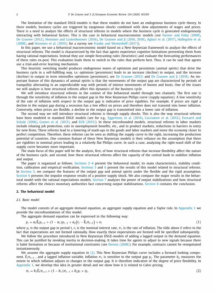
We then simulated our calibrated model over 20 0 0 periods for different standard deviations of the exogenous shocks

in inflation (while keeping the standard deviation of output shocks constant) and computed the standard deviations of the


Fig. 1. Standard deviations of the simulated output gap and inflation.

Fig. 2. Autocorrelations of inflation and output gap in behavioral model.

simulated output gap and inflation. We did this consecutively for increasing standard deviations of the inflation shocks.

We assumed an inflation target of 2%. The results are shown in Fig. 1 . This shows the standard deviation of the simulated

output gap and inflation for different standard deviations in the inflation shocks (and for a standard deviation of the output

gap equal to 0.5). We observe that with a standard deviation of the shocks in inflation and of output gap of 0.5 we come

very close to the empirically observed standard deviations of the output gap and inflation of Table 2 . It is also interesting

to observe that while we assume the same standard deviation in the shocks of output and inflation the model produces a

significantly higher standard deviation of the output gap than of inflation. This is also confirmed empirically. Thus, we do

not need to assume that the exogenous shocks in the output gap are higher than the shocks in inflation to produce this

result. It should be mentioned that the parameter values in Table 1 ensure local stability of the steady state.

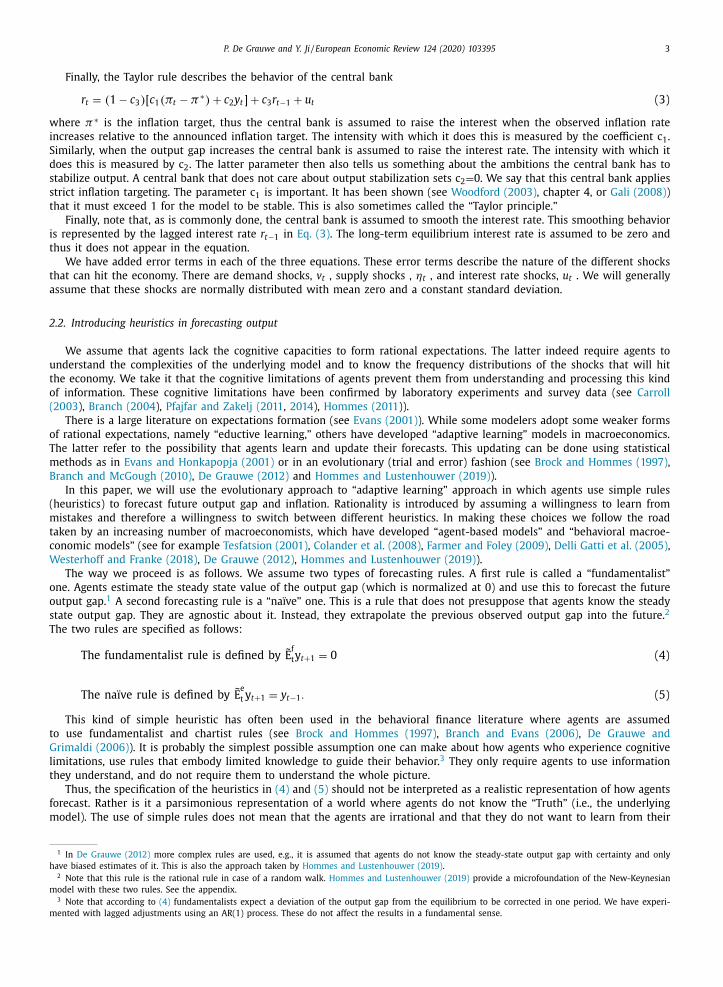
Next, we look at the serial correlation. Our behavioral model produces strong serial correlation in the output gap and

inflation despite the fact that the shocks in Eqs. (1) –(3) are i.i.d. Thus, the model produces serial correlation endogenously.

In Fig. 2 , we show this feature by presenting the autocorrelation function of the output gap and inflation as simulated in

the model. We observe strong and persistent autocorrelation. 8

8 One could object to this empirical evidence that the large shocks observed in the output gaps can also be the result of large exogenous shocks. The

claim that is made here is not that the economy cannot sometimes be hit by large shocks (it often is), but that a theory that can explain large movements

in output gaps only as a result of large exogenous shocks is an incomplete one. This creates an opening for a theory like ours that can explain large

movements in the output gap (fat tails) endogenously.


Fig. 3. Observed autocorrelations in inflation, UK and US.

Fig. 4. Observed autocorrelations in output gap, UK and US.

In the next step we compared the autocorrelations obtained from our model with the empirical ones. In Figs. 3 and 4 we

show the empirical autocorrelations of inflation (see Fig. 3 ) and output gap (see Fig. 4 ) for the UK and the US. We observe

that our model predicts a pattern of serial correlations of inflation and output gap that resembles those obtained in reality.

Finally, we compared these autocorrelations with those obtained from the New Keynesian model with rational expecta-

tions. We do this by taking the aggregate demand and supply Eqs. (1) and (2) together with the Taylor rule (3) and solved

it under rational expectations, using the same calibrations of the parameters and assuming i.i.d. shocks. We then simulated

this model and computed the autocorrelation functions. The results are shown in Fig. 5 . We find much less autocorrelation

than in the behavioral model. In addition, the NK-model with RE assumptions falls far short from producing the serial cor-

relations that are observed in reality. It has become customary in the DSGE-literature to “solve” this is by assuming that the

shocks are serially correlated (see Smets and Wouters (2003) ).

5. Structural reforms and business cycle

5.1. Modeling structural reforms

We use the behavioral model developed in the previous section to study how different types of structural reforms affect

the macroeconomy. We will distinguish between two types of structural reforms.

The first type has the effect of increasing the price flexibility. Such an increase in flexibility increases the coefficient

b 2 in the New Keynesian Philips curve (see Eq. (2) ), i.e., when structural reform increases flexibility we will observe that

changes in the output gap have a stronger effect on prices, so that the rate of inflation reacts strongly to such changes. In


Fig. 5. Autocorrelations of inflation and output gap in the NK-RE model.

Appendix 1 we show how this coefficient can be derived from the microfoundations of the model.

b 2 =

( 1 − θ ) ( 1 − βθ )

θ

σ ( 1 − α) + ϕ + α

1 − α + αε (36)

where β , σ , ϕ, ɛ and α are parameters in the consumer demand and firm production functions. The coefficient θ relates

to “Calvo pricing”. Each firm is assumed to reset prices in period t with probability 1 − θ , where θ is the fraction of firms

that keep their prices fixed. Thus, θ can be considered as a measure of prices stickiness. In general, we can say that when

1 − θ = 0 there is perfect rigidity, i.e., θ = 1 , and all firms keep their price fixed. In that case, as can be seen from (36) ,

b 2 = 0. As 1 − θ increases, b 2 increases monotonically. A fully flexible economy is one where 1 − θ = 1 , i.e. all firms adjust

their prices in each period. In that case b 2 = ∞ . We will characterize a rigid economy to be one where b 2 is close to 0, and

a flexible economy one where b 2 is close to 1.

The second type of structural reforms (e.g. bringing more competition in labor market, increasing the degree of partici-

pation in the labor market, extending the retirement age) has the effect of raising potential output. In Appendix 1 we focus

on one such mechanism. This is the wage markup. For example, in a labor market dominated by labor unions the wage

markup is high. Structural reforms that aim at bringing more competition in the labor market tend to reduce the markup.

These structural reforms therefore can be seen as producing a positive supply shock (a negative shock in ηt in Eq. (2) ).

We will analyze these two types of structural reforms consecutively, but we will also focus on their interactions.

5.2. The power of animal spirits: rigidity versus flexibility

We can now use the behavioral model first to analyze how different degrees of price flexibility affect the dynamics of

the business cycles. We simulated the model over 20 0 0 periods. We present the results in the time domain and in the

frequency domain. Fig. 6 shows the movements of the output gap and animal spirits in the time domain (left hand side

panels). We selected a sample of 200 periods (quarters) that is representative of the full simulation. The right hand side

panel shows the output gap and animal spirits in the frequency domain for the full 20 0 0 periods.

We select a low value for the flexibility parameter ( b 2 = 0.05). We observe that the model produces waves of optimism

and pessimism (animal spirits) that can lead to a situation where everybody becomes optimist ( S t = 1) or pessimist ( S t = -1).

These waves of optimism and pessimism are generated endogenously, i.e., the i.i.d. shocks are transformed into serially cor-

related (persistent) movements in market sentiments. They arise because optimistic (pessimistic) forecasts are self-fulfilling

and therefore attract more agents into being optimists (pessimists).

As can be seen from the left hand side panels, the correlation of these animal spirits and the output gap is high, reaching

0.95. Underlying this correlation is the self-fulfilling nature of expectations. When a wave of optimism is set in motion, this

leads to an increase in aggregate demand (see Eq. (1) ). This increase in aggregate demand leads to a situation in which

those who have made optimistic forecasts are vindicated. This attracts more agents using optimistic forecasts. This leads to

a self-fulfilling dynamics in which most agents become optimists. It is a dynamics that leads to a correlation of the same

beliefs. The reverse is also true. A wave of pessimistic forecasts can set in motion a self-fulfilling dynamics leading to a

downturn in economic activity (output gap). At some point most of the agents have become pessimists.

In De Grauwe (2012) and De Grauwe and Ji (2018) empirical evidence is provided indicating that output gaps are highly

correlated with empirical measures of animal spirits. It is shown that when performing causality tests on US and the Euro-

zone data one cannot reject the hypothesis that the output gap Granger causes the index of business confidence, and vice

versa one cannot reject the hypothesis that the index of business confidence Granger causes the US and Eurozone output


Fig. 6. Output and animal spirits ( b 2 = 0.05, rigid case).

gap during 1999–2015. Thus, there is a two-way causality between market sentiments and the output gap. This is also what

our model predicts.

The right hand side panels show the frequency distribution of output gap and animal spirits. We find that the output

gap is not normally distributed, with excess kurtosis and fat tails. A Jarque–Bera test rejects normality of the distribution

of the output gap. The origin of the non-normality of the distribution of the output gap can be found in the distribution

of the animal spirits. We find that there is a concentration of observations of animal spirits around 0. This means that

much of the time there is no clear-cut optimism or pessimism. We can call these “normal periods.” There is also, however,

a concentration of extreme values at either -1 (extreme pessimism) and + 1 (extreme optimism). These extreme values

of animal spirits explain the fat tails observed in the distribution of the output gap. The interpretation of this result is

as follows. Our model produces self-fulfilling movements of optimism and pessimism (animal spirits). When agents with

optimistic forecasts happen to be more numerous than those with pessimistic forecasts, this will tend to raise the output

gap. The latter in turns validates those who made optimistic forecasts. This then attracts more agents to become optimists.

(See Devenov and Welch (1996) for similar mechanisms in financial markets). When the market is gripped by a self-fulfilling

movement of optimism (or pessimism) this can lead to a situation where everybody becomes optimist (pessimist). This then

also leads to an intense boom (bust) in economic activity.

Let us now assume that structural reforms increase the degree of flexibility in the economy. As indicated earlier, this

increases the parameter b 2 in the New Keynesian Philips curve (see Eq. (2) ). We now analyze how the increase in flexibility

affects the nature of the business cycle. We set the parameter b 2 = 1 and compare the results with those obtained in a rigid

economy (see Fig. 6 ). The results of the simulation of a flexible economy are shown in Fig. 7 .


Fig. 7. Output and animal spirits ( b 2 = 1, flexible case).

Compared to the case of the rigid economy, we find two interesting results. First, in a flexible economy the power of

animal spirits is significantly reduced. The extreme levels of optimism ( S t = 1) or pessimism ( S t = -1) become less frequent.

On the other hand, the concentration of the animal spirits around zero is much higher.

Second, as can be seen in the left panel of Fig. 7 , the correlation between the output gap and animal spirits appears to

be lower. We find a correlation of 0.85. This contrasts with 0.95, which is obtained in the rigid economy. As a result, the

output gap in Fig. 7 is also less volatile. We find that in the flexible economy the standard deviation of the output gap is

0.5. The corresponding standard deviation in the rigid economy is 1.7, a significant difference.

Thus, we find that an economy that is more flexible is less prone to the boom-bust nature of the business cycle produced

by waves of optimism and pessimism (animal spirits) than a more rigid economy. The underlying reason for this result can

be explained as follows. Let us assume that a boom in economic activity emerges: the output gap becomes positive. In a

flexible economy this increase in the output gap has a strong positive effect on inflation (according to Eq. (2) ). As the central

bank attaches a high weight to inflation in the Taylor rule it react strongly by raising the interest rate (according to Eq. (3) ).

This tends to reduce the intensity of the boom. When in a rigid economy the output gap increases this will have a weaker

effect on inflation, leading the central bank to raise the interest rate less than in a flexible economy. As a result, the boom

in economic activity is stronger, which intensifies positive animal spirits so that in the rigid economy the same initial shock

in the output gap is more likely to generate an intense boom followed by a bust. A rigid economy will therefore be more

prone to booms and bust driven by animal spirits than a flexible economy.

It is interesting to note that in a rigid economy not only output will be more volatile than in a flexible economy but

inflation also. We find that in the rigid economy the standard deviation of inflation is 0.95 while it is 0.64 in a flexible


Fig. 8. Correlation between output and animal spirits.

economy. The reason is that in a rigid economy the central bank does less stabilization after a shock in the output gap

thereby allowing animal spirits to intensify the boom bust nature of the business cycle. This in the end also tends to make

the rate of inflation more volatile.

Note that this result is solely due to the fact that the central bank attaches more importance to the stabilization of

inflation than of the output gap. In a flexible economy this will naturally lead to more stabilization of the business cycle

than in the rigid economy. It follows that in a rigid economy there is a need for the central bank to attaching a greater

importance in stabilizing the output gap. We return to this issue when we discuss optimal monetary policies in rigid and

flexible economies.

The previous analysis compared the results obtained for two different values of b 2 . In order to obtain more general

results, it is important to subject the analysis to a more precise sensitivity analysis. The way we do this is to compute the

correlation between output and animal spirits for different values of the level of the flexibility of the economy. The results

are shown in Fig. 8 . Each point represents the correlation coefficient (see Fig. 8 ) and kurtosis (see Fig. 9 ) obtained from

a 20 0 0-period simulation with a given value of the flexibility parameter (horizontal axes). The red lines are the best fit

between these points. We find that the correlation between output gap and animal spirits decreases when b 2 increases (i.e.,

the flexibility of the economy increases). The correlation starts at around 0.95 when b 2 is close to zero and then decreases

to 0.85 when b 2 reaches 1. When b 2 increases further to 5, the correlation decreases slowly to about 0.5.

As flexibility reduces the power of animal spirits, this also leads to fewer extreme values of the output gap. As a result,

we are more likely to have a normally distributed output gap. Fig. 8 informs us about this relationship. When b 2 = 0 the

average kurtosis exceeds 4.5, which is too high for the output gap to be normally distributed. The average kurtosis gradually

declines as b 2 increases and approaches 3 when b 2 = 5 suggesting that the output gap is normally distributed.

5.3. Comparing business cycle dynamics in behavioral and DSGE-models

One important feature of our behavioral model is its prediction that the distribution of the output gap is non-normal,

i.e. that it has excess kurtosis and fat tails. Thus, the behavioral model predicts that the business cycle is characterized by

periods of tranquility (excess kurtosis) and booms and busts (fat tails). This dynamics of the business cycle is produced

endogenously. It can be interesting to compare this result with the dynamics obtained in a similar New-Keynesian model

assuming Rational Expectations (DSGE-model). As before, we use our basic model consisting of the aggregate demand (1) ,

aggregate supply Eq. (2) , and Taylor rule (3) and solve it for rational expectations (using the same parameters as those used

in the behavioral model). We do this for both the rigid economy ( b 2 = 0.05) and the flexible economy ( b 2 = 1). We show the

results in Fig. 10 . We find that in both the rigid and flexible case the distribution is normal. Kurtosis is around 3 and a

Jarque–Bera test cannot reject normality. A NK-model under rational expectations does not produce a boom-bust dynamics.

It should be remembered that the shocks we impose are normally distributed (i.i.d.). Thus, the only way the NK-model with

RE can produce non-normality in the output gap is by assuming that the exogenous shocks driving the aggregate demand

and supply equations are non-normal. This is not a very satisfactory theory of the business cycle as it requires us to explain

the boom-bust dynamics by shocks originating from outside the macro-economy.


Fig. 9. Kurtosis of output gap.

Fig. 10. Frequency distribution output gap.

Note: kurtosis rigid economy = 2.91; kurtosis flexible economy = 3.01.

The existence of non-normality in the distribution of the output gap (and output growth) has been confirmed empirically

for most OECD countries. See also Fagiolo et al. (2008) , Fagiolo et al. (2009) , and De Grauwe and Ji (2016) . Ascari et al.,

(2015) find that RBC and NK models cannot generate the fat tails observed in the data (which our model can) . 9

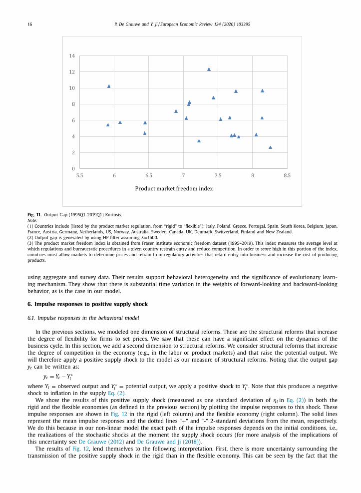
In Fig. 11 , we show the kurtosis of the output gap for a number of OECD-countries during 1995–2019. These kurtoses

vary a great deal and all of them (except New Zealand which has the highest degree of product market freedom) are well

above 3, suggesting that the output gaps in most industrialized countries are not normally distributed.

Recently, Cornea et al. (2019) estimated a similar behavioral model of inflation dynamics with heterogeneous firms,

with two groups of price setters, fundamentalists and random walk believers. The authors estimate the switching model

9 This diminishing return applies to the effects structural reforms have on the variance of output and inflation. It is not related to a similar diminishing

return of the long term effects of structural reforms on the mean growth rate of the economy.


Fig. 11. Output Gap (1995Q1-2019Q1) Kurtosis.

Note:

(1) Countries include (listed by the product market regulation, from “rigid” to “flexible”): Italy, Poland, Greece, Portugal, Spain, South Korea, Belgium, Japan,

France, Austria, Germany, Netherlands, US, Norway, Australia, Sweden, Canada, UK, Denmark, Switzerland, Finland and New Zealand.

(2) Output gap is generated by using HP filter assuming λ= 1600.

(3) The product market freedom index is obtained from Fraser institute economic freedom dataset (1995–2019). This index measures the average level at

which regulations and bureaucratic procedures in a given country restrain entry and reduce competition. In order to score high in this portion of the index,

countries must allow markets to determine prices and refrain from regulatory activities that retard entry into business and increase the cost of producing

products.

using aggregate and survey data. Their results support behavioral heterogeneity and the significance of evolutionary learn-

ing mechanism. They show that there is substantial time variation in the weights of forward-looking and backward-looking

behavior, as is the case in our model.

6. Impulse responses to positive supply shock

6.1. Impulse responses in the behavioral model

In the previous sections, we modeled one dimension of structural reforms. These are the structural reforms that increase

the degree of flexibility for firms to set prices. We saw that these can have a significant effect on the dynamics of the

business cycle. In this section, we add a second dimension to structural reforms. We consider structural reforms that increase

the degree of competition in the economy (e.g., in the labor or product markets) and that raise the potential output. We

will therefore apply a positive supply shock to the model as our measure of structural reforms. Noting that the output gap

y t can be written as:

y t = Y t − Y ∗t where Y t = observed output and Y ∗t = potential output, we apply a positive shock to Y ∗t . Note that this produces a negative

shock to inflation in the supply Eq. (2) .

We show the results of this positive supply shock (measured as one standard deviation of ηt in Eq. (2) ) in both the

rigid and the flexible economies (as defined in the previous section) by plotting the impulse responses to this shock. These

impulse responses are shown in Fig. 12 in the rigid (left column) and the flexible economy (right column). The solid lines

represent the mean impulse responses and the dotted lines “+ ” and “-” 2-standard deviations from the mean, respectively.

We do this because in our non-linear model the exact path of the impulse responses depends on the initial conditions, i.e.,

the realizations of the stochastic shocks at the moment the supply shock occurs (for more analysis of the implications of

this uncertainty see De Grauwe (2012) and De Grauwe and Ji (2018) ).

The results of Fig. 12 , lend themselves to the following interpretation. First, there is more uncertainty surrounding the

transmission of the positive supply shock in the rigid than in the flexible economy. This can be seen by the fact that the


Fig. 12. Impulse responses to positive supply shock. (For interpretation of the references to color in this figure, the reader is referred to the web version

of this article.)

dotted red lines are farther apart in the rigid than in the flexible economy. In addition, it takes longer in the former for this

uncertainty to die out than in the latter. Put differently, the impulse responses to the same supply shock are more sensitive

to initial conditions in the rigid than in the flexible economy. This is related to the result we found in the previous section.

We noted there that in the rigid economy the power of animal spirits is higher than in the flexible economy. These animal

spirits create the potential for fat tails in the output gap. As a result, initial conditions (including the state of animal spirits)

have as stronger effect on the transmission of the supply shock in the rigid economy. All this creates greater uncertainty

about the transmission of a supply shock. It also implies that given the high variance in the impulse responses one cannot


even be sure about the sign of this transmission. This result is in line with a wide literature on how structural reforms affect

the economy (see e.g., Hausman and Velasco (2005) .

Second, the duration it takes to adjust to the long-term equilibrium is different in the two types of economy. It takes

longer in the rigid economy to adjust to the long-term equilibrium compared to the flexible economy where the adjustment

takes only a few quarters.

Third, we observe that the short-term impact of the positive supply shock on output and inflation are higher in the

flexible economy than in the rigid one. In addition, the central bank reacts more strongly by lowering the interest rate in

the flexible economy than in the rigid one.

How can these results be interpreted? The positive supply shock has a stronger negative effect on inflation in the flexible

economy than in the rigid one because prices react more to the increase in excess supply generated by the positive shock

in potential output. This leads to a strong decline in inflation in the flexible economy. Since the central bank attaches a high

weight to inflation, it is led to reduce the rate of interest significantly more in the flexible than in the rigid economy. This

creates a stronger boom in aggregate demand in the flexible economy than in the rigid one. Thus, in a flexible economy, the

same supply shock initiated by structural reforms leads to a stronger boom in economic activity than in a rigid economy

because the central bank, observing a steep drop in inflation, is induced to fuel this boom more than in a rigid economy.

We assume, of course, that the central bank does not adjust its monetary policy rule (Taylor rule) when the economy moves

from a rigid to a flexible one.

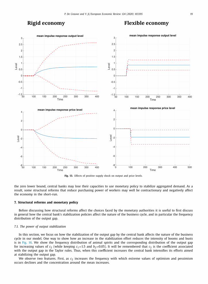
It is also important to analyze the long-term impact of the supply shock on the level of output in the rigid and flexible

economies. We obtain these by computing the cumulative effects of the supply shock on the output gap and on inflation.

This yields the effects on the output level and the price level. We show the results in Fig. 13 .

Again, we find that the uncertainty surrounding the effects of the supply shock to be much greater in the rigid than in

the flexible economy, and that we cannot even be sure of the sign of this effect. We also find that the level effects of the

positive supply shock in the flexible economy are somewhat higher than in the rigid economy. These differences, however,

are quite small, so that it is better to conclude that given the uncertainty surrounding the effects of structural reforms

there is no significant difference in the long term effects of a supply shock in the rigid versus the flexible economy. A note

of warning is important here. Our model is not designed to analyze long-term effects in a satisfactory way as it does not

incorporate long-term capital accumulation.

6.2. Impulse responses under rational expectations

To understand what the behavioral features bring in the analysis, we compare the results of our model to a rational ex-

pectation (RE) model. The RE model consisting of the aggregate demand function (1) , the aggregate supply function (2) and

the Taylor rule (3) can be solved assuming rational expectations (RE). We do this in the present section using the same

parameter values as those used in the behavioral model. In both models we assume the same distributions of the stochastic

shocks (i.i.d. with zero mean and std = 0.5) and compare the results obtained under RE with the results of our behavioral

model. We perform this exercise both for the rigid economy ( b 2 = 0.05) and the flexible economy ( b 2 = 1). We focus on the

impulse responses following a positive supply shock. We show these impulse responses in Figs. 14 and 15 . These should be

compared to the impulse responses to a positive supply shock in our behavioral model (see Figs. 12 and 13 ).

As in the behavioral model, the output and price level effects of a positive supply shock are higher in a flexible than in

a rigid economy.

The differences between the two models are the following. First, we find that the rational expectations model produces

weaker output and inflation effects of the same supply shocks than the behavioral model. This difference is related to the

fact that the animal spirits tend to amplify the supply shock. This holds both in the rigid and the flexible economy. As a

result, the level effects (output and price levels) are higher in the behavioral model.

Second, we find that the economy takes a much longer time to adjust to its long-term equilibrium in the behavioral

model than in the rational expectations model. This difference is large: if the economy is rigid it takes approximately fifty

periods in the behavioral model to go back to equilibrium versus less than ten periods in the rational expectations model.

Another way to put this difference is in terms of half-lives. It takes about twenty-one periods for the behavioral model to

reach half of the distance to the long-run equilibrium after the supply shock. In the rational expectations model this half-life

is approximately four periods.

Third, in contrast to the behavioral model, there is no uncertainty about the impulse responses in the RE-model. In the

latter, there is no sensitivity to initial conditions. Put differently, the im pulse responses are not influenced by the timing of

the supply shock. They are the same for all realizations of the stochastic shocks. If there is uncertainty in the RE-model this

finds its origin in the uncertainty surrounding the estimated coefficients. The latter uncertainty, however, is also present in

the behavioral model. Thus, in the behavioral model there are two types of uncertainty: one is due to the uncertainty about

the parameters of the model (as in the RE-model); the other is the result of the fact that the impulse responses are sensitive

to initial conditions.

A recent development in the DSGE literature related to structural reforms (see for example Eggertson et al. (2014) and

Sajedi (2017) ) reaches similar conclusions as ours, i.e., that structural reforms in the form of reducing the mark-ups in the

labor and product markets may not generate positive impacts in the short run. Unrelated to uncertainty and the initial

conditions we stress in the behavioral model, this literature stresses that in a recession when the nominal interest rate hits


Fig. 13. Effects of positive supply shock on output and price levels.

the zero lower bound, central banks may lose their capacities to use monetary policy to stabilize aggregated demand. As a

result, some structural reforms that reduce purchasing power of workers may well be contractionary and negatively affect

the economy in the short-run.

7. Structural reforms and monetary policy

Before discussing how structural reforms affect the choices faced by the monetary authorities it is useful to first discuss

in general how the central bank’s stabilization policies affect the nature of the business cycle, and in particular the frequency

distribution of the output gap.

7.1. The power of output stabilization

In this section, we focus on how the stabilization of the output gap by the central bank affects the nature of the business

cycle in our model. One way to show how an increase in the stabilization effort reduces the intensity of booms and busts

is in Fig. 16 . We show the frequency distribution of animal spirits and the corresponding distribution of the output gap

for increasing values of c 2 (while keeping c 1 = 1.5 and b 2 = 0.05). It will be remembered that c 2 is the coefficient associated

with the output gap in the Taylor rules. Thus, when this coefficient increases the central bank intensifies its efforts aimed

at stabilizing the output gap.

We observe two features. First, as c 2 increases the frequency with which extreme values of optimism and pessimism

occurs declines and the concentration around the mean increases.


Fig. 14. Impulse responses to positive supply shock in a rigid economy ( b 2 = 0.05).

Fig. 15. Impulse responses to positive supply shock in a flexible economy ( b 2 = 1).

Second, the variability of the output gap declines significantly. This can be seen on the horizontal axis of the distribution

of the output gap. With low c 2 the output gaps varies between much larger values than when c 2 is high. Thus, the intensity

of output stabilization (increases in c 2 ) has a double effect: it reduces the variability of the output gap and it reduces the

frequency with which extreme booms and bust occur as a result of extreme variation of animal spirits.

7.2. Structural reforms and monetary policy tradeoffs

How does the flexibility as measured by parameter b 2 affect the policy tradeoffs of the monetary authorities? This is the

question we analyze in this section. It will allow us to answer the question of whether structural reforms aimed at making

the economy more flexible facilitate the policy choices of the monetary authorities.

We derive a monetary policy tradeoff that measures how increasing the intensity with which the central bank stabilizes

the output gap affects its choice between inflation and output volatility. We do this by varying the parameter c 2 in the Taylor

rule and compute the standard deviations of output gap and inflation for increasing values of c 2 . We repeat the exercise for

different values of the flexibility parameter, b 2 .

Fig. 17 presents the Taylor output parameter on the horizontal axis and the standard deviation of the output gap on the

vertical axis. We find negatively sloped curves. When rigidity is high (i.e., b 2 is low) these lines are located higher than

when rigidity is low (i.e., b is high). Also, as b increases the curves become flatter. Thus, in a very rigid economy, initial
2 2


Fig. 16. Frequency distribution animal spirits and output gap ( c 1 = 1.5 and b 2 = 0.05).


Fig. 17. Standard deviation of output gap and the Taylor output parameter.

Fig. 18. Standard deviation of inflation and the Taylor output parameter.

stabilization efforts have a much stronger negative effect on output volatility. In other words, it pays more to stabilize in a

rigid economy.

Fig. 18 shows the relationship between the output stabilization parameter c 2 and inflation volatility for different values of

b 2 . Here we find another type of non-linearity. When c 2 increases (starting from 0) the effect is to reduce inflation volatility.

This goes on up to a point. When this point is reached, further attempts at output stabilization lead to increases in inflation

variability. This point is reached faster in the rigid economy (low b 2 ). When the economy becomes more flexible this point

is shifted to the right and the positive effect of more stabilization on inflation volatility is reduced.

Combining Figs. 17 and 18 allows us to derive the trade-offs. These are shown in Fig. 19 . We observe that when b 2 increases (i.e., the economy becomes more flexible), the tradeoffs shift downward and toward the origin. This means that

more flexibility improves the tradeoff of the monetary authorities, i.e., they can achieve lower levels of output and inflation

volatility with the application of the same interest rate policies. We also observe that there are diminishing returns of

flexibility: for sufficiently high values of b 2 the downward shifts produced by further increases in flexibility become very

small. 10 This is reached for values of b exceeding 1.
2
10 This diminishing return applies to the effects structural reforms have on the variance of output and inflation. It is not related to a similar diminishing

return of the long term effects of structural reforms on the mean growth rate of the economy.


Fig. 19. Output and inflation tradeoff.

We also observe from Fig. 19 that there is an upward sloping part of the tradeoffs. In order to understand this, it is

useful to start from A on the uppermost tradeoff (corresponding to a rigid economy). This is the point obtained when the

central bank does not stabilize output, i.e., c 2 = 0. When c 2 increases (i.e., the central bank increases its output stabilization

effort) we move down along the curve. This leads to a “win-win” situation: by increasing its output stabilization the central

bank reduces the volatility of output and inflation. When this is the case the central bank does not have to make a choice:

more output stabilization can be achieved without cost in terms of more inflation volatility. At some point, however, when

the central bank continues to increase its stabilization effort it reaches the negatively sloped part of the tradeoff, implying

that it has to make a choice between output and inflation stabilization. The reason why we obtain this result is that at its

initial stage output stabilization has the effect of reducing the fat tails in the distribution of the output gap (the booms and

busts). Put differently, it reduces the power of animal spirits. As long as these are intense, output stabilization reduces both

the volatility of inflation and output. When these fat tails are sufficiently lowered, the standard result of a negative trade-off

reappears.

We also observe that when b 2 is small the “win-win” situation is very pronounced. This result can be interpreted as

follows. In a rigid economy the power of animal spirits is high, producing fat tails in the output gap, i.e. extreme outcomes

in the movements of the business cycle. When this is the case the power of output stabilization by the central bank is

strong as it helps to reduce the intensity of animal spirits. When the economy becomes more flexible animal spirits become

weaker and so is the power of the central bank to stabilize the business cycle.

8. Conclusion

In this paper, we have analyzed how different types of structural reforms affect the economy. We have used a New

Keynesian behavioral macroeconomic model to perform this analysis. This is a model characterized by the fact that agents

experience cognitive limitations preventing them from having rational expectations. Instead they use simple forecasting rules

(heuristics) and evaluate the forecasting performances of these rules ex-post. This evaluation leads them to switch to the

rules that perform best. This heuristic switching model produces endogenous waves of optimism and pessimism (animal

spirits) that drive the business cycle in a self-fulfilling way, i.e., optimism (pessimism) leads to an increase (decline) in

output, and the increase (decline) in output in term intensifies optimism (pessimism).

Exercises evaluating the impact of structural reforms have been done using standard DSGE-models (see e.g.,

Eggertsson et al. (2014) . Doing this in the framework of a behavioral macroeconomic model is a novel attempt.

We considered two types of structural reforms. The first one increases price flexibility; the second one that increases

competition in the labor market and hence raises potential output in the economy. We find that structural reforms that

increase price flexibility can have profound effects on the dynamics of the business cycle. In particular in a more flexible

economy (more price flexibility) the power of animal spirits is reduced and so is the potential for booms and busts in the

economy. This has to do with the fact that in more flexible economies prices have a greater role to play in adjustments to

emerging disequilibria. Since the central bank attaches a greater importance to inflation stabilization than output stabiliza-

tion, this has the effect that the central bank will tend to stabilize more in a flexible than in a rigid economy. This reduces


the amplitude of the business cycles and as a result creates less scope for waves of optimism and pessimism in producing

booms and busts.

Our behavorial model also generates interesting policy implications. We found that the degree of flexibility affects the

tradeoffs faced by the central bank. When the central bank increases its efforts at stabilizing output, this first leads to a

win-win situation, i.e., effort s at st abilizing output reduce both output and inflation volatility. The origin of this win-win

situation lies in the existence of fat tails in the distribution of the output gap (extreme events). By stabilizing the output

gap, the central bank reduces the fat tails and the power of animal spirits. As a result, extreme booms and busts are reduced

in frequency and intensity and this has the effect of reducing both the volatility of output and inflation. This effect is absent

in the RE-model where animal spirits play no role. This win-win situation, however, disappears when the central bank has

reduced the power of the fat tails sufficiently. It will then face a negative tradeoff between output and inflation volatile.

Finally, we studied the tradeoffs of the central bank when the degree of flexibility in the economy increases. We found

that in a more flexible economy (as measured by the b 2 -parameter) the tradeoffs the central banks face improve. This

means that the central bank can achieve less volatility of inflation and output by applying the same interest rate policies

in a flexible economy as compared to a more rigid economy. There are, however, diminishing returns to this effect, i.e., at

some point more flexibility stops improving the tradeoffs.

Central bankers have a tendency to reduce their responsibility for stabilizing output by arguing that it is the responsibility

of the political authorities to introduce structural reforms that will lead to a more flexible economy. This then will reduce

the need for active stabilization policies. This point has often been made by policymakers at the helm of the European

Central Bank. We have found that this argument is only half true. It is true that more flexibility makes it easier to stabilize

the economy. At the same time, however, the responsibility of the central bank for stabilizing output remains a strong one.

We have found that for different degrees of flexibility the central bank can reduce the power of animal spirits by active

stabilization policies. This power is the strongest in a rigid economy but does not disappear when the economy gets more

flexible. The central bank cannot shed its responsibility of stabilizing an otherwise unstable economy.

More research should be performed to analyze the interplay of structural reforms and behavioral assumptions in macroe-

conomic modeling. First, there is a need to extend the model so as to allow for the analysis of long-term effects of structural

reforms that increase the flexibility of the economy. Second, it would be desirable to add a labor market to the model. This

will allow us to enlarge the dimension of structural reforms programs in the model and to analyze unemployment as well

as output and inflation. Finally, adding a financial sector into the model would make it possible to better understand how

that sector adds to the need to stabilize the macroeconomy and how this can best be done.

Appendix 1. Microfoundations of the basic behavioral model

We show that the aggregate demand and supply equations used in the main text can be microfounded on individual

utility maximization of households and profit maximization of firms even while we assume that expectations are set using

the heuristics of fundamentalists and extrapolators.

A.1.1. Aggregate demand

Let us start by modeling the demand side of the model. This will be based on the maximization of individual’s utility of

consumption over an infinite horizon. In contrast with the canonical model presented in the previous chapter we will allow

for heterogeneity of individual agents.

The individual consumer, i , maximizes the following function over an infinite horizon:

E 0

∞ ∑

t=0

βt U

(C i t , N

i t

)(A1)

where β is discount factor, U is the utility function, which is assumed to have the same form every period and every agent,

C i t is consumption of agent i in period t and N

i t is hours worked by agent i .

The budget constraint faced by consumer i is

P t C i t + Q t B

i t ≤ B

i t−1 + W t N

i t − T t (A2)

where B i t is the quantity of one period discount bond purchased by agent i in period t and maturing in t + + 1; Q t is price

of bond, P t is the price of consumption goods, W t is the wage rate and T t is a lump-sum tax

First order condition for consumer’s optimum (Euler equation)

−U n,t

U c,t =

W t

P t (A3)

Q t = β ˜ E i t

[U c,t+1

U c,t

P t

P t+1

](A4)

where ˜ E i is the forecast made by agent i in period t using the behavioral heuristic explained in the main text.
t


Assume a CES utility function

U

(C i t , N

i t

)=

C i, 1 −σt

1 − σ− N

i, 1+ ϕ t

1 + ϕ

(A5)

First order optimality conditions can then be written as

W t

P t = C i, σt N

i,ϕ t (A6)

Q t = β ˜ E i t

[ (C i t+1

C i t

)−σP t

P t+1

]

(A7)

Log-linearization yields ( A6 ) the labor supply equation

w t − p t = σ c i t + ϕn

i t (A8)

where lower case letters are natural logarithms. We will not use this labor supply equation as we currently assume full wage

flexibility. In Section A.1.2.1 , we will impose conditions that allow some monopoly power of household to set the wage and

some rigidities will be introduced too.

Similarly log-linearization ( A7 ) yields the consumption equation (Euler equation) for individual i :

c i t =

˜ E i t c i t+1 −

1

σ

(r t − ˜ E i t πt+1 − ρ

)(A9)

where the interest rate r t = −log ( Q t ) , the inflation rate πt = log P t+1 − log P t and ρ = − log β .

We follow Hommes and Lustenhouwer (2016) in assuming that the probability to follow a particular forecasting rule

(heuristic) in period t is the same across agents, and independent of the heuristic they followed in the past. This follows

from the fact that agents are not inherently different, but that each of them is confronted with the same choice between

being following a naïve or fundamentalist forecasting rule. In addition, as in Hommes and Lustenhouwer (2016) , we assume

“agents know that all agents have the same probability to follow a particular heuristic in the future, and that they know that

consumption decisions only differ between households insofar as their expectations are different”. In that case households’

forecasts about their individual consumption must be the same as their forecast of the consumption of any other individual.

It follows that the individual’s forecast of his own consumption will coincide with the forecast of aggregate consumption:

˜ E i t c i t+1 =

˜ E i t c t+1 (A10)

where c t + 1 is aggregate consumption.

This allows us to rewrite the Euler equation as

c i t =

˜ E i t C t+1 − 1

σ

(r t − ˜ E i t πt+1 − ρ

). (A11)

In equilibrium aggregate demand = aggregate supply of output, i.e., c t = y t We assume that agents understand market clearing. As a result, their forecast of consumption coincides with their fore-

cast of output. We can write

˜ E i t c t+1 =

˜ E i t y t+1 (A12)

As a result, we can write ( A11 ) as

c i t =

˜ E i t y t+1 − 1

σ

(r t − ˜ E i t πt+1 − ρ

)(A13)

Aggregating this expression over all agents i , and using the market clearing condition, yield

y t =

˜ E t y t+1 − 1

σ

(r t − ˜ E t πt+1 − ρ

). (A14)

This is the aggregate demand equation we use in the main text (without inertia). Thus, the aggregate demand equation

we use in our behavioral model can be microfounded. In order to do so, we had to make some assumptions, in particular

that individual agents know that the probability of using a particular forecasting rule in period t is the same across agents.

As a result the individual agent’s forecast of his own consumption coincides with the forecast of aggregate consumption.

This does not seem to be a particularly strong assumption requiring great cognitive capacities of agents.

The aggregate demand equation used in the main text includes a lagged output gap. Such a lagged output gap can be

introduced by assuming habit formation (see , Fuhrer (20 0 0) and Dennis (20 08) ). We then have a utility function of the

form

E 0

∞ ∑

t=0

βt U

(C i t , H

i t , N

i t

)(A15)

where H

i is the habit stock of agent i .
t


Assuming the habit stock obeys the expression

H

i t = ηC i t−1

where we assume external habit formation (see Dennis (2008) . This allows us to derive an aggregate demand equation of

the form (see Dennis (2008) )

y t =

1

1 + η˜ E

t

y t+1 +

η

1 + ηy t−1 − 1

σ

(r t − ˜ E t πt+1 − ρ

)(A16)

which is the aggregate demand equation used in the main text where

a 1 =

1

1 + η

and

1 − a 1 =

η

1 + η

A.1.2. Aggregate supply

A.1.2.1. Staggered price setting

There is a continuum of firms each producing a differentiated good j in monopolistically competitive markets.

The production function of firm j is specified as follows:

Y j t = A t N

j, 1 −αt (A17)

We introduce a “New-Keynesian” feature in the model which is that prices are sticky. It is customary to assume so-called

Calvo pricing. We show that it is possible to microfound our behavioral model under the same assumptions about price

rigidity as in the standard DSGE-models.

Calvo pricing assumes that each firm will reset prices in period t with probability 1 − θ , where θ is the fraction of firms

that keep their prices fixed. Thus, θ can be considered as a measure of prices stickiness.

Each period firms that have drawn the “Calvo lottery ticket,” i.e. are allowed to change their price, will set that price, P ∗t , such that it maximizes the current value of profits generated while that price remains effective

Firms maximize expected profits with respect to P ∗t ∞ ∑

k =0

( βθ ) k ˜ E j t

[P j, ∗t Y j

t+ k/t − �t+ k

(Y j

t+ k/t

)](A18)

subject to the demand constraints

Y j t+ k/t

=

(P ∗t

P t+ k

)−ε

C j t+ k (A19)

Where �t+ k ( Y j

t+ k/t ) is the cost function, Y

j

t+ k/t is the output of the firm that last reset its price in period t.

The first order condition of an optimum is:

∞ ∑

k =0

( βθ ) k ˜ E j t

[Y j

t+ k/t

(P j, ∗t − Mψ

j

t+ k/t

)]= 0 (A20)

where ψ t+ k/t is the marginal cost in t + k for firm that last reset its price in t and M is markup, i.e.

M =

ε

ε − 1

(A21)

Log-linearizing and solving for the price, yields

p j, ∗t = μ + ( 1 − βθ )

∞ ∑

k =0

( βθ ) k ˜ E j t

[mc j

t+ k/t + p j

t+ k ]

(A22)

where μ is the desired markup, m c t+ k/t is the (real) marginal cost. Note that m c t+ k/t + p t+ k is the nominal marginal cost.

Eq. (A22) says that firms resetting their price will choose a price equal to desired (equilibrium) markup plus expected

marginal costs that will prevail as long as the price is effective (is not changed).

Using

πt = ( 1 − θ ) ( p ∗t − p t−1 ) (A23)

we obtain

π j t = λ

∞ ∑

k =0

βk ˜ E j t

[ mc j

t+ k ]

(A24)

where b 2 =

( 1 −θ )( 1 −βθ) θ

1 −α1 −αε and

mc j

t+ k is the marginal cost expressed as a deviation from the steady state.


Thus, when the deviation of marginal cost from steady state is positive a fraction of prices is adjusted upwards, leading

to more inflation.

Just as in the case of the demand equation the discrete choice model of the selection of forecasting rules implies that

˜ E j t

[ mc j

t+ k ]

=

˜ E j t [ mc t+ k ] . (A25)

Finally, we can rewrite

π j t = β ˆ E j t [ πt+1 ] + λ mc t (A26)

Aggregating over all firms j (see Hommes and Lustenhouwer (2016) , we obtain

πt = β˜ E t [ πt+1 + λm c t ] . (A27)

The last step consists in relating marginal cost to the output gap

πt = β ˜ E t [ πt+1 ] − λ ˆ μt (A28)

where ˆ μt = μt − μ = − mc t and λ =

( 1 −θ )( 1 −βθ) θ

1 −α1 −α+ α ε

A.1.2.2. staggered wage setting

In a way analogous to the assumptions on the price-setting constraints facing firms, assume that for each period only a

fraction 1 − θw

of households drawn randomly from the population reoptimize their posted nominal wage. We now consider

how households choose the wage for their labor when allowed to reoptimize that wage. The household will choose w t at

period t in order to maximize.

˜ E i t

{

∞ ∑

t=0

(βθw

) k U

(C i t+ k | t , N

i t+ k | t

)}

(A29)

Where C i t+ k | t and N

i t+ k | t repectively denote the consumption and labor supply in period t + k of a household i that last rest

its wage in period t. Note that the utility generated under any other wage set in the future is irrelevant from the point of

view of the optimal setting of the current wage, and thus can be ignored in (A29) .

Given the utility function specified in ( A5 ), the first-order condition associated with the problem above is given by

∞ ∑

k =0

( βθw

) k ˜ E i t

{N t+ k | t U c

(C i t+ k | t , N

i t+ k | t

)( w t

p t+ k − M w

MR S t+ k | t

)}= 0 (A30)

MRS i t+ k | t = −U n ( C i t+ k | t ,N i t+ k | t )

U c ( C i t+ k | t ,N i t+ k | t ) denote the marginal rate of substitution between consumption and labor in period t + k for the

household resetting the wage in period t and M w

=

ε w 1 −ε w

. Note that ɛ w

measures the elasticity of substitution among labor

varieties.

Log-linearizing ( A30 ) around the steady state (zero inflation) yields the following approximate wage setting rule

w

∗t = μw + ( 1 − βθw

)

∞ ∑

k =0

( βθw

) k ˜ E i t

{mr s t+ k | t + p t+ k

}(A31)

Where μw is household markup. mr s t+ k | t is the (log) marginal rate of substitution in period t + k for a household that

reset its wage in period t.

Using πw

t = ( 1 − θw

) ( w t − w t−1 )

We obtain:

πw

t = β ˜ E i t {πw

t+1

}− λw

μw

t (A32)

Where λw

=

( 1 −θw )( 1 −βθw ) θw ( 1+ ε w ϕ ) and ˆ μw

t = μw

t − μw

Just as in the demand equation and price setting equations, the discrete choice model of the selection of forecasting rules

(concerning wages inflation) implies that we are able to aggregate over all households i , we obtain

πw

t = β ˜ E t {πw

t+1

}− λw

μw

t (A33)

A.1.3. Aggregate supply equation

To obtain the Philips curve we use in our model, we following Gali (2008) :

Define real wage ω t = w t − p t , real natural wage ω

n t = w

n t − p n t , and real wage gap ˜ ω t = ω t − ω

n t ,

ˆ μw

t = ˜ ω t −(σ +

ϕ

1 − α

)y t


ˆ μt = − ˜ ω t − α

1 − αy t

Referring to Eq. (A27) , we obtain the New Keynesian Philips curve specified in our model:

πt = β ˜ E t [ πt+1 ] − λ ˆ μt

= β ˜ E t [ πt+1 ] + λ(

˜ ω t +

α

1 − αy t

)= β ˜ E t [ πt+1 ] + λ

(ˆ μw

t +

(σ +

ϕ

1 − α

)y t +

α

1 − αy t

)= β ˜ E t [ πt+1 ] + λ

(σ ( 1 − α) + ϕ + α

1 − α

)y t + λ ˆ μw

t

= β ˜ E t [ πt+1 ] + b 2 y t + λ ˆ μw

t

where b 2 =

( 1 −θ )( 1 −βθ) θ

σ ( 1 −α)+ ϕ+ α1 −α+ αε

We assume that wage is fully flexible, ˆ μw

t = 0 , then inflation is not influenced by the labor market πt = β ˜ E t [ πt+1 ] + b 2 y t .

We consider the following two extreme scenarios:

(1) If price is fully flexible ( θ→ 0), λ → ∞ , b 2 → ∞ , then inflation responds strongly to output gap. In the simulation, we

set b 2 = 0.05 as an example.

(2) If θ= 1, λ= 0, b 2 = 0 , extreme rigidity, then inflation does not react to output gap, i.e. πt = β ˜ E t [ πt+1 ] . In the simulation,

we set b 2 = 1 as an example.

Note that in order to obtain an aggregate supply equation with a lagged inflation, as we have in the main text an

indexation scheme has to be introduced. In such an indexation scheme the prices that in the context of the Calvo rule

cannot be optimized in period t are indexed to inflation in period t-1. This is done in Smets and Wouters (2003) . It is

shown there that with indexation the aggregate supply curve is of the form

πt =

β

1 + β∧

˜ E t [ πt+1 ] +

ξ

1 + β∧

πt−1 + b 2 y t + λ ˆ μw

t

where ∧ expresses the degree of indexation. When ∧ = 0 there is no indexation and we obtain an aggregate supply curve

without lagged inflation. When ∧ = 1 we have full indexation and we obtain the aggregate supply curve used in the main

text. In that case the coefficients on the forward looking and lagged inflation add up to 1.

References

Agliari, A. , Massaro, D. , Pecora, N. , Spelta, A. , 2017. Inflation targeting, recursive inattentiveness, and heterogeneous beliefs. J. Money Credit Bank. 49 (7),

1587–1619 .

Assenza, T. , Bao, T. , Hommes, C. , Massaro, D. , 2014. Experiments on expectations in macroeconomics and finance. In: Duffy, J. (Ed.). In: Experiments inMacroeconomics (Research in Experimental Economics), 17. Emerald Group Publishing Limited, Bingley, West Yorkshire, pp. 11–70 .

Assenza, T. , Heemeijer, P. , Hommes, C.H. , Massaro, D. , 2020. Managing self-organization of expectations through monetary policy: a macro experiment. J.Monet. Econ. in press .

Anderson, S. , de Palma, A. , Thisse, J.-F. , 1992. Discrete Choice Theory of Product Differentiation. MIT Press, Cambridge, MA . Ascari, G. , Fagiolo, G. , Roventini, A. , 2015. Fat-Tail distributions and business-cycle models. Macroecon. Dyn. 19 (2), 465–476 .

Blanchard, O., 2018. On the future of macroeconomic models. Oxford Rev. Econ. Policy 5 January 2018 34 (1–2), 43–54. doi: 10.1093/oxrep/grx045 .

Blattner, T.S. Margaritov, E., 2010. Towards a robust monetary policy rule for the euro area. Branch, W.A. , 2004. The theory of rationally heterogeneous expectations: evidence from survey data on inflation expectations. Econ. J. 114 (497), 592–621 .

Branch, W. , Evans, G. , 2006. Intrinsic heterogeneity in expectation formation. J. Econ. Theory 127, 264–295 . Brazier, A. , Harrison, R. , King, M. , Yates, T. , 2008. The danger of inflation expectations on macroeconomic stability: heuristic switching in an overlapping

generations monetary model. Int. J. Central Bank. 32, 2428–2452 . Brock, W. , Hommes, C. , 1997. A rational route to randomness. Econometrica 65, 1059–1095 .

Cacciatore, M. , Duval, R. , Fiori, G. , 2012.. Short-term gain or pain. A DSGE Model-Based Analysis of the Short-Term Effects of Structural Reforms in Labour

and Product Markets. OECD Economics Department Working paper no. 948 . Cacciatore, M. , Fiori, G. , Ghironi, F. , 2016. Market deregulation and optimal monetary policy in a monetary union. J. Int. Econ 99, 120–137 .

Carroll, C.D. , 2003. Macroeconomic expectations of households and professional forecasters. Quart. J. Econ. 118 (1), 269–298 . Colander, David , Howitt, Peter , Kirman, Alan , Leijonhufvud, Axel , Mehrling, Perry , 2008. Beyond DSGE models: toward an empirically based macroeconomics.

Amer. Econ. Rev. 98 (2), 236–240 . Cornea, A. , Hommes, C.H. , Massaro, D. , 2019. Behavioral heterogeneity in U.S. inflation dynamics. J. Bus. Econ. Statist. 37 (2), 288–300 .

De Grauwe, P. , Grimaldi, M. , 2006. The Exchange Rate in a Behavioural Finance Framework. Princeton University Press .

De Grauwe, P. , 2012. Lectures on Behavioral Macroeconomics. Princeton University Press . De Grauwe, P., Ji, Y., 2016. International correlation of business cycles in a behavioral macroeconomic model, CEPR, Discussion Paper, April.

De Grauwe, P., Ji, Y., 2018. Inflation targets and the zero lower bound in a behavioural macroeconomic model. Economica doi: 10.1111/ecca.12261 . Delli Gatti, D. , Di Guilmi, C. , Gaffeo, E. , Giuloni, G. , Gallegati, M. , Palestrini, A. , 2005. A new approach to business fluctuations: heterogeneous interacting

agents, scaling laws and financial fragility. J. Econ. Behav. Organ. 56, 489–512 . Dennis, R., 2008. Consumption habits in a new Keynesian business cycle model, Federal Reserve Bank of San Francisco, Discussion Paper.

Devenov, A. , Welch, I. , 1996. Rational herding in financial economics. Eur. Econ. Rev. 40 (3–5), 603–615 issue .

Eggertsson, G. , Ferrero, A. , Raffo, A. , 2014. Can structural reforms help Europe? J. Monet. Econ. 61, 2–22 . European Central Bank (E.C.B.), 2015. Progress with structural reforms across the euro area and their possible impacts, Economic Bulletin, 2.

Evans, G.W., 2001. Expectations in macroeconomics: adaptive versus eductive learning. Revue Écon. 52 (3), 573–582. doi: 10.2307/3502871 . Evans, G. , Honkapohja, S. , 2001. Learning and Expectations in Macroeconomics. Princeton University Press, p. 421 .

Everaert, L., Schule, W., 2006. Structural reforms in the Euro area: economic impact and role of synchronization across markets and countries, InternationalMonetary Fund, No. 6-137.

http://refhub.elsevier.com/S0014-2921(20)30027-1/sbref0001























https://doi.org/10.1093/oxrep/grx045







































https://doi.org/10.1111/ecca.12261















https://doi.org/10.2307/3502871





Fagiolo, G. , Napoletano, M. , Roventini, A. , 2008. Are output growth rate distributions fat-tailed: evidence for OECD-countries. J. Appl. Econ. 23, 639–669 . Fagiolo, G. , Napoletano, M , Piazza, M. , Roventini, A. , 2009. Detrending and the distributional properties of U.S. output time series. Econ. Bull. 29 (4) .

Farmer, J.D. , Foley, D. , 2009. The economy needs Agent- Based Modelling. Nature 460, 6 85–6 86 . Franke, R. , Westerhoff, F. , 2017. Taking stock: a rigorous modelling of animal spirits in macroeconomics. J. Econ. Surv. 31 (5), 1152–1182 .

Fuhrer, J. , 20 0 0. Habit formation in consumption and its implications for monetary-policy models. Amer. Econ. Rev. 90 (3), 367–390 . Galí, J. , 2008. Monetary Policy, Inflation and the Business Cycle. Princeton University Press, p. 203 .

Gomes, S. , Jacquinot, P. , Mohr, M. , Pisani, M. , 2013. Structural reforms and macroeconomic performance in the Euro area countries: a model-based assess-

ment. Int. Finance 16 (1), 23–44 . Hallegatte, S. , Ghil, M. , Dumas, P. , Hourcade, J.C. , 2008. Business cycles, bifurcations and chaos in a neo-classical model with investment dynamics. J. Econ.

Behav. Organ. 67 (1), 57–77 . Hausmann, R. , Rodrik, D. , Velasco, A. , 2005. Growth Diagnostics. Harvard University, Mimeo .

Hommes, C. , 2011. The heterogeneous expectations hypothesis: some evidence from the lab. J. Econ. Dyn. Control 35 (1), 1–24 Elsevier . Hommes, C., Lustenhouwer, J., 2016. Managing heterogeneous and unanchored expectations: a monetary policy analysis, Tinbergen Institute, Rotterdam,

Working Paper. Hommes, C. , Lustenhouwer, J. , 2019. Inflation targeting and liquidity traps under endogenous credibility. J. Monet. Econ. 107, 48–62 .

Hommes, C. , Massaro, D. , Weber, M. , 2019. Monetary policy under behavioral expectations: theory and experiment. Eur. Econ. Rev. 118, 193–212 .

Hommes, C.H. , 2020. Behavioral and experimental macroeconomics and policy analysis: a complex systems approach. J. Econ. Lit. in press . Kahneman, D. , 2002. Maps of bounded rationality: a perspective on intuitive judgment and choice. Nobel Prize Lecture. Stockholm December 8also pub-

lished in American Economic Review, 2003 . Kirman., A. , 1992. Whom or what does the representative individual represent? J. Econ. Perspect. 6 (2), 117–136 Spring .

Kryvtsov, O., Petersen, L., 2013. Expectations and monetary policy: experimental evidence. Bank of Canada, No. 2013-44 Kukacka, J., Jang, T.S., Sacht, S., 2018. On the estimation of behavioral macroeconomic models via simulated maximum likelihood. Available at SSRN 3299450.

McCallum, B.T. , Nelson, E. , 1999. Performance of operational policy rules in an estimated semiclassical structural model. In: Monetary Policy Rules. Univer-

sity of Chicago Press, pp. 15–56 . Pfajfar, D., B. Zakelj, 2011., inflation expectations and monetary policy design: evidence from the laboratory, Tilburg University, CentER Discussion Paper

2011-091. Pfajfar, D. , Zakelj, B. , 2014. Experimental evidence on inflation expectation formation. J. Econ. Dyn. Control 44, 147–168 .

Sajedi, R. , 2017. Fiscal consequences of structural reform under constrained monetary policy. In: Proceedings of the Workshop on Structural Reforms andEuropean Integration. European Institute, London School of Economics 8th May .

Smets, F. , Wouters, R. , 2003. An estimated dynamic stochastic general equilibrium model. J. Eur. Econ. Assoc. 1, 1123–1175 .

Tesfatsion, L. , 2001. Introduction to the special issue on agent-based computational economics. J. Econ. Dyn. Control 25 (3–4), 281–293 . Wren-Lewis, S., 2018. Ending the microfoundations hegemony. Oxford Rev. Econ. Policy 5 January 2018 34 (1–2), 55–69. doi: 10.1093/oxrep/grx054 .

Westerhoff, F. , Franke, R. , 2018. Agent-based models for economic policy design: two illustrative examples. In: Chen, S.-H., Kaboudan, M., Du, Y.-R. (Eds.),The Oxford Handbook of Computational Economics and Finance. Oxford University Press, Oxford, pp. 520–558 .

Woodford, M. , 2003. Interest and Prices: Foundations of a Theory of Monetary Policy. Princeton University Press .






























































https://doi.org/10.1093/oxrep/grx054

http://refhub.elsevier.com/S0014-2921(20)30027-1/othref0011





structural reforms, animal spirits and monetary policies

Documents