structural equation modeling structural equation modeling (sem) melinda k. higgins, ph.d. 13 april...
TRANSCRIPT

Structural Equation Modeling
Structural Equation Modeling (SEM)
Melinda K. Higgins, Ph.D.
13 April 2009

Structural Equation Modeling
SEM – descriptions
• SEM is a collection of statistical techniques that allow a set of relationships between one or more IVs (independent variables) (either continuous or discrete) and one or more DVs (dependent variables) (also either continuous or discrete).
• SEM is also called causal modeling; causal analysis; simultaneous equation modeling; analysis of covariance structures; analysis of moments; path analysis or confirmatory factor analysis [last 2 are special types of SEM]
• (example) When you combine EFA (exploratory factor analysis) with multiple regression, you have SEM.
• Some recommend you begin with confirmatory factor analysis (where applicable), then evaluate the various “paths/regression relationships” and, finally, put it all together into one SEM model. [D. Garson]

Structural Equation Modeling
SEM – advantages and disadvantages
• ADV – When relationships among factors are examined the relationships are free from measurement error (because error has been estimated and removed leaving only common variance).
• ADV – Thus, reliability of measurement can be accounted for explicitly within the analysis by estimating and removing the measurement error.
• ADV – When phenomena of interest are complex and multidimensional, SEM is the only analysis that allows complete and simultaneous test of all the relationships.
• DISADV – with increased flexibility comes increased complexity (and demands for larger sample sizes).

Structural Equation Modeling
“Types” of SEM
• Measurement Model/Confirmatory Factor Analysis
• Path Analysis
• Structural “Regression” Analysis
• Latent Change (or Growth) Models

Structural Equation Modeling
Confirmatory Factor Analysis

Structural Equation Modeling
Path Model

Structural Equation Modeling
SEM (CFA and Path Combined)

Structural Equation Modeling
Latent Change (Growth) Model

Structural Equation Modeling
SEM - goal
• Develop a model the “fits” the data (based on variance/covariance matrix)
• H0: Model “fits” the data (“fit” function defined that compares sample cov matrix, S, to predicted cov matrix )
• Ha: Model does not “fit” the data
• Test via a 2 - want a non-significant test (p-val >> 0.05)
• 2 - is calculated by comparing estimated predicted covariance to sample covariance [ideally = 0, no difference between S and ]

Mediators – How to test for …
[Preacher, Hayes] – 3 approaches:(1) Baron, Kenny:
(i) Y = i1 + cX(ii) M = i2 + aX(iii) Y = i3 + c’X + bM
(2) Sobel Test
(i) calculate ab (assumption Normal Distribution)
(ii) calculate sab = sqrt (b2sa2 + a2sb
2 + sa2sb
2)(iii) divide ab/sab compare to N(0,1) critical values
(3) Bootstrap sampling distribution for ab
IV DV
Med
c
a b
c’
“suffers from low power”

Example [Preacher,Hayes]
Therapy Satisfaction
Attribution
c
a b
c’
“An investigator is interested in the effects of a new cognitive therapy on life satisfaction after retirement. Residents of a retirement home diagnosed as clinically depressed are randomly assigned to receive 10 sessions of a new cognitive therapy or an alternative method. After session 8, the “positivity of attributions” the residents make for a recent failure experience is assessed. After session 10, the residents are given a measure of life satisfaction (questionnaire).”
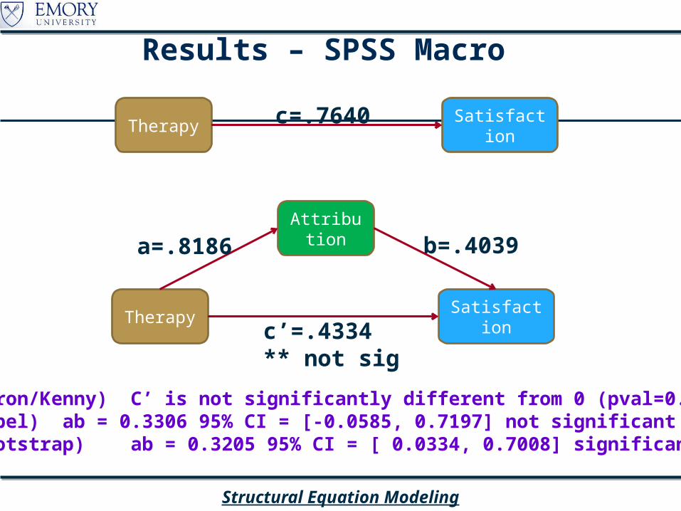
Results – SPSS Macro
Therapy Satisfaction
Attributiona=.8186 b=.4039
c’=.4334** not sig
Therapy Satisfactionc=.7640
(Baron/Kenny) C’ is not significantly different from 0 (pval=0.1897)(Sobel) ab = 0.3306 95% CI = [-0.0585, 0.7197] not significant(Bootstrap) ab = 0.3205 95% CI = [ 0.0334, 0.7008] significant

Example (cont’d) – Mediation Using Structural Equation Modeling (SEM) via AMOS
See http://davidakenny.net/cm/mediate.htm and tutorial (video and sound) at http://amosdevelopment.com/video/indirect/flash/indirect.html

SEM (cont’d)
AMOS-boot 95%CI [0.075, 0.788]Macro-boot 95%CI [0.0334, 0.7008]
Structural Equation Modeling
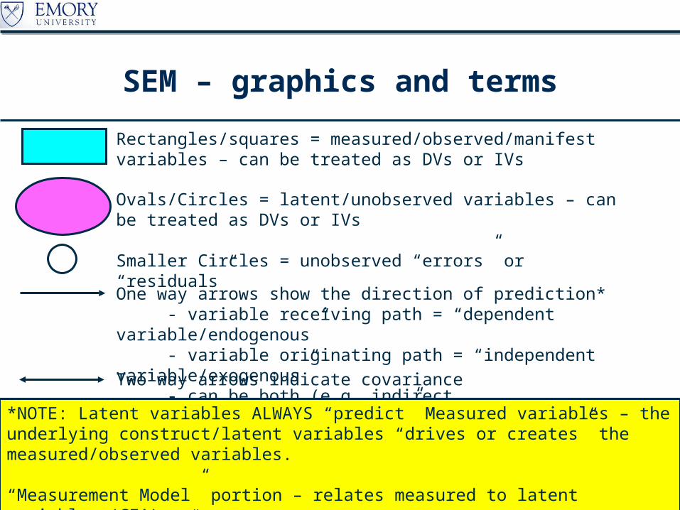
SEM – graphics and terms
Rectangles/squares = measured/observed/manifest variables – can be treated as DVs or IVs
Ovals/Circles = latent/unobserved variables – can be treated as DVs or IVs
Smaller Circles = unobserved “errors” or “residuals”
One way arrows show the direction of prediction* - variable receiving path = “dependent variable/endogenous” - variable originating path = “independent variable/exogenous” - can be both (e.g. indirect effect/mediator)
Two way arrows indicate covariance
*NOTE: Latent variables ALWAYS “predict” Measured variables – the underlying construct/latent variables “drives or creates” the measured/observed variables.
“Measurement Model” portion – relates measured to latent variables (CFA)“Structural Model” portion – relates constructs (usually) to each other

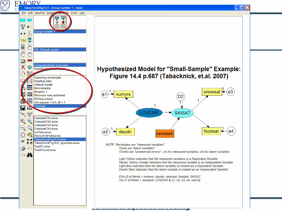
Example Data (Tabachnick et.al. Fig 14.4)
5 continuous measured variables:• NUMYRS – number of years participant has skied• DAYSKI – total number days person has skied• SNOWSAT – Likert scale measure of overall satisfaction with snow conditions• FOODSAT – Likert scale measure of overall satisfaction with quality of food at resort• SENSEEK – Likert scale measure of degree of sensation seeking
2 hypothesized latent variables:• LOVESKI – Love of Skiing• SKISAT – Ski Trip Satisfaction
It is hypothesized that:1. Love of Skiing “predicts” number of year skied and number of days skied2. Ski Trip Satisfaction “predicts” degree of satisfaction with snow conditions and food quality
at resort.3. Love of Skiing and degree of sensation seeking “predict” level of Ski Trip Satisfaction
Figure on next page shows these relationships and the hypothesized model

numyrs
dayski
snowsat
foodsat
e11
e21
e31
e41
1
LOVESKI SKISAT
senseek
D21
1
Hypothesized Model for "Small-Sample" Example:Figure 14.4 p.687 (Tabacknick, et.al. 2007)
NOTE: Rectangles are "measured variables" Ovals are "latent variables" Circles are "unobserved errors" - e's for measured variables, d's for latent variables
Light Yellow indicates that the measured variables is a Dependent Variable Darker Yellow-Orange indicates that the measured variable is an Independent Variable Light Blue indicates that the latent variables is treated as a Dependent Variable Darker Blue indicates that the latent variable is treated an an Independent Variable
DVs (5 of them) = numyrs; dayski; snowsat; foodsat; SKISAT IVs (7 of them) = senseek; LOVESKI & e1, e2, e3, e4, and d2
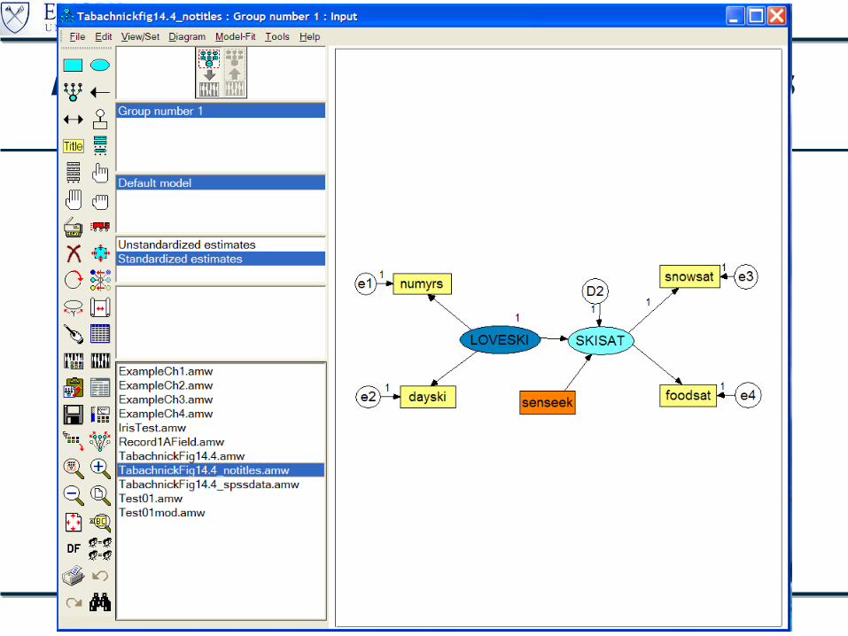
AMOS - Amos is short for Analysis of MOment Structures.
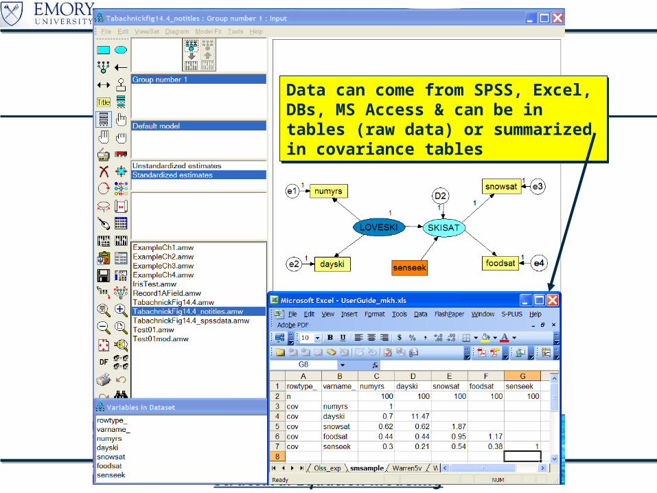
Data can come from SPSS, Excel, DBs, MS Access & can be in tables (raw data) or summarized in covariance tables
Data can come from SPSS, Excel, DBs, MS Access & can be in tables (raw data) or summarized in covariance tables

Dependent Variables = “endogenous”
Dependent Variables = “endogenous”
Independent Variables = “exogenous”
Independent Variables = “exogenous”
Observed vars =“measured variables”
Unobserved vars =“latent variables”
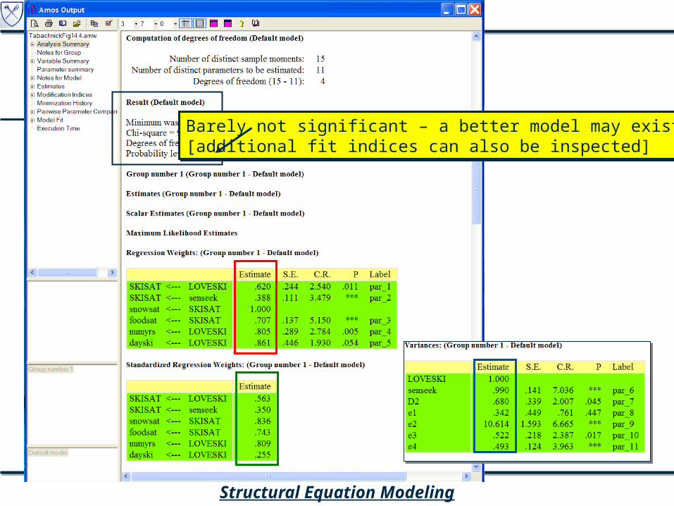
Barely not significant – a better model may exist?[additional fit indices can also be inspected]Barely not significant – a better model may exist?[additional fit indices can also be inspected]

Numbers in circled in blue are variances
Numbers in circled in red are (unstandardized) regression coefficients
Unstandardized Estimates
1. NUMYRS and DAYSKI are both significant indictors of LOVESKI [see Tabachnick, et.al. p.695 for z-score tests on regression parameters – all have pval < or = to 0.05]
2. FOODSAT is a significant indicator of SKISAT3. [Since SKISAT SNOWSAT was set=1, this significance cannot be determined – rerun
with SKISAT FOODSAT set=1]4. SENSEEK is a significant indicator of SKISAT5. LOVESKI is a significant indicator of SKISAT

Standardized Estimates
Now all variances = 1 [not shown]
Numbers in circled in green are (standardized) regression coefficients
1. Standardized regression coefficients can be compared to each other since the “scales” of the variables have been removed.
2. E.g. can compare that NUMYRS is a stronger indicator (.81) of LOVESKI than DAYSKI (.26) although both were tested to be significant indicators.
3. Likewise both SNOWSAT and FOODSAT are almost equivalently strong indicators of SKISAT
4. LOVESKI while significant is a weaker indicator (.56) of SKISAT followed by SENSEEK with an even lower standardized regression weight of 0.35.

Structural Equation Modeling
6 rules
1. All variances of independent variables are model parameters
2. All covariances between independent variables are model parameters
3. All factor loadings are model parameters
4. All regression coefficients between observed or latent variables are model parameters
5. Variances and covariances between dependent variables and/or covariances between dependent variables and independent variables are NEVER model parameters (because these variances and covariances are themselves explained in terms of other model parameters)
6. For each latent variable, the “metric” of its latent “scale” needs to be set. [usually either the variance = constant (1) or the path leaving the latent variable = constant (1).]

Structural Equation Modeling
Measurement ModelConfirmatory Factor Analysis
CHECK 6 RULES
(1) 8 error variances (e1 e8) and 3 factor variances (1)
(2) 3 factor covariances(3) 8 factor loadings(4) n/a – no regression relationships(5) No 2-way arrows between DVs nor
between IV-DV.(6) Metric of 3 factors is “fixed” by setting
their variances = 1 (see (1) above).
So, there are 8 + 3 + 8 = 19 “free” parameters to estimate

Structural Equation Modeling
Degrees of Freedom(“Identification”)
For a model to be “identified,” there must be the same or fewer number of parameters than non-redundant elements in the covariance matrix (i.e. degrees of freedom >= 0).
DF = [P(P+1)/2] – number of parameters to be estimated
DF (example) = [8(9)/2] – 19 = 36 – 19 = 17 degrees of freedom
NOTE: If DF=0, the model is said to be saturated.


Structural Equation Modeling

Structural Equation Modeling
References
• Tabachnick, Barbara G.; Fidell, Linda S. “Using Multivariate Statistics,” 5th edition, Pearson Education Inc., 2007. {“Chapter 14: SEM” good worked examples – with discussion of covariance math}
• Raykov, Tenko; Marcoulides, George. “A First Course in Structural Equation Modeling.” Lawrence Erlbaum Associates Publishers, New Jersey, 2000. {good examples with LISREL and EQS codes and some info on AMOS}
• Kline, Rex. “Principles and Practice of Structural Equation Modeling.” The Guilford Press, New York, 1998. {some info on AMOS, EQS and LISREL}
• Kaplan, David. “Structural Equation Modeling – Foundations and Extensions.” 2nd edition, SAGE Publications, Los Angeles, 2009. {more advanced text, but good indepth discussions}
• Duncan, T; Duncan, S; Strycker, L; Li, F; Alpert, A. “An Introduction to Latent Variable Growth Curve Modeling: Concepts, Issues and Applications.” Lawrence Erlbaum Associates Publishers, New Jersey, 1999. {also good worked examples with EQS and LISREL codes}

Structural Equation Modeling
VIII. Statistical Resources and Contact Info
SON S:\Shared\Statistics_MKHiggins\website2\index.htm
[updates in process]
Working to include tip sheets (for SPSS, SAS, and other software), lectures (PPTs and handouts), datasets, other resources and references
Statistics At Nursing Website: [website being updated] http://www.nursing.emory.edu/pulse/statistics/
And Blackboard Site (in development) for “Organization: Statistics at School of Nursing”
Contact
Dr. Melinda Higgins
Office: 404-727-5180 / Mobile: 404-434-1785