Structural Equation Modeling

Mgmt 291Lecture 4

Model Specification & Data PreparationOct. 19, 2009

What we have:1) National Level Research Government capability

(Governance) Corruption – Political Instability – Property Right

– Rule Regulation

Foreign Direct Investment

Data – need to merger datasets ?

Shanshan Qiu

2) Firm Level Research 1) Earning

Stock price

??? 2) Football team

Abilities => Score Points

John Bae

Matthew Feldmann

3) Individual Level Research 1) Why starting a businessInterests - Belief => Starting

2) Consuming a green product

WealthValue => Organic Food ConsumptionLife-style

Laura Huang

Hannah Oh

3) Analysts behavior by Joshua

A few issues on first assignment: 1) Theory -> Operationalization need to be completed

Theory & Concepts -> Data & Variables

Questions -> Hypotheses

Concepts and Variables linked

2) Confirmative Approach vs. Exploratory Approach need to be clear

Clear Theory-backed hypotheses

Strictly confirmative ? (maybe some exploratory elements added

later are fine)

Usually start with confirmative if theories are strong.

OR completely exploratory.

3) Clear Strategies Needed Extend Replicate previous research Test some theories empirically

Review literature – some critique – are necessary.

(need to know how important your research is, what your contribution is)

4) Need SEM Type of Questions

(that can NOT be handled by OLS regression) Mediation effects Latent Variables Non-recursive

Correlated Disturbances (Errors or Residuals)

- model comparison (15 fit indexes)

SEM Types ofHypotheses

Or Causality Questions

Time precedence ? Direction – (need SEM to rule out other direction)

Partialed out

(panel studies, disturbance – non-deterministic)

Or Group Comparison Questions

Measurement Invariance Cross Groups

Structure Invariance Cross Groups

Example of Literature Review Literature review – a lot of research on

determinants of economic growth AND determinants of democracy, a few article starting to argue that DEMOCRACY needs to be treated as latent var.

Lack of empirical study of the feedback loop of economic growth and democracy.

Indirect impacts of determinants are rare.

Example of SEM Questions Democracy is a latent variable with

Freedom House indicator, Polity indicator, Polyarchy Indicator and others (FH, ACLP in our data)

democracy and economic growth may be affected by each other.

The impacts of economic development on democracy may be indirect.

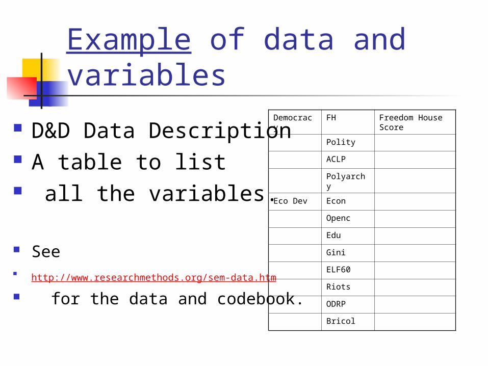
Example of data and variables

D&D Data Description A table to list all the variables.

See http://www.researchmethods.org/sem-data.htm for the data and codebook.

Democracy

FH Freedom House Score

Polity

ACLP

Polyarchy

Eco Dev Econ

Openc

Edu

Gini

ELF60

Riots

ODRP

Bricol

For Second Assignment move to model specification Hypotheses or theories <-> model (to be represented by

diagrams)

Hypotheses or Model Spec Generation Exploratory way use partial correlation to generate model spec

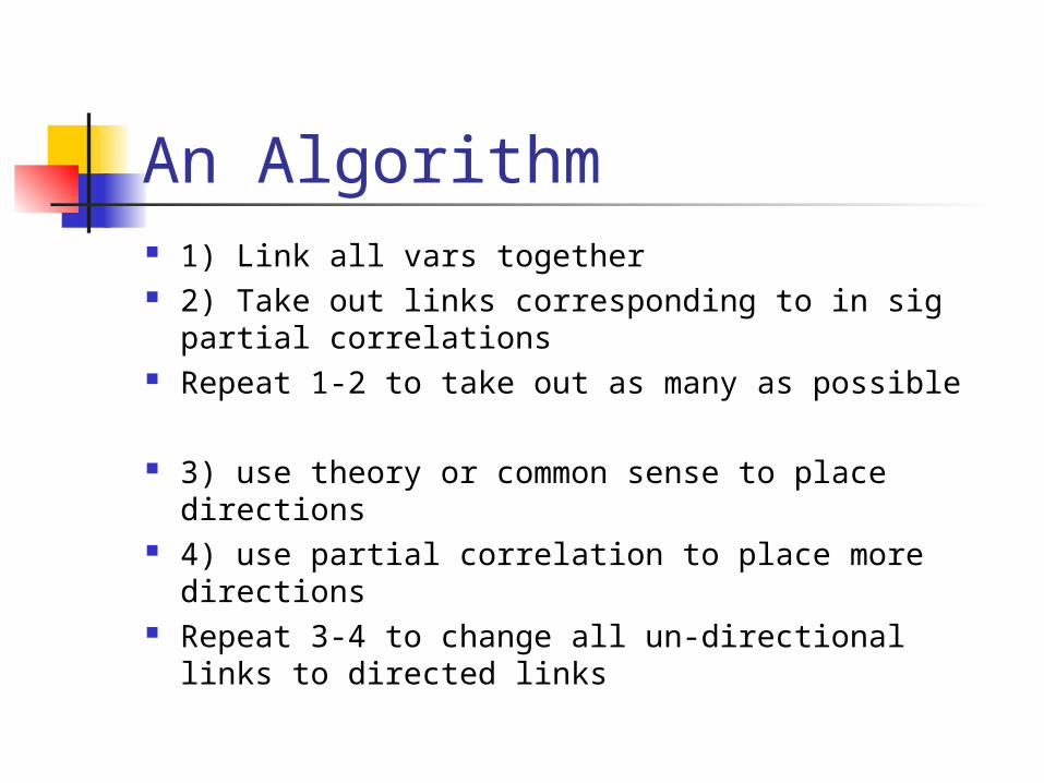
An Algorithm 1) Link all vars together 2) Take out links corresponding to in sig partial

correlations Repeat 1-2 to take out as many as possible

3) use theory or common sense to place directions

4) use partial correlation to place more directions Repeat 3-4 to change all un-directional links to

directed links

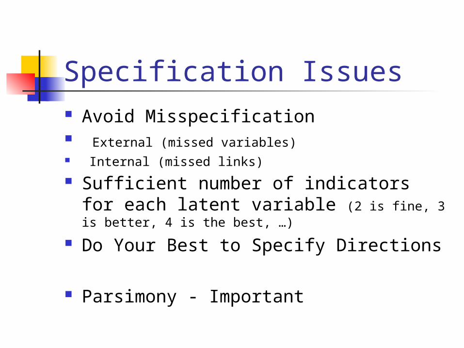
Specification Issues Avoid Misspecification External (missed variables) Internal (missed links)

Sufficient number of indicators for each latent variable (2 is fine, 3 is better, 4 is the best, …)

Do Your Best to Specify Directions

Parsimony - Important

Misspecification Problems -> Biases

Over-estimationSuppression

(depends on the correlation between vars in the equation and vars omitted

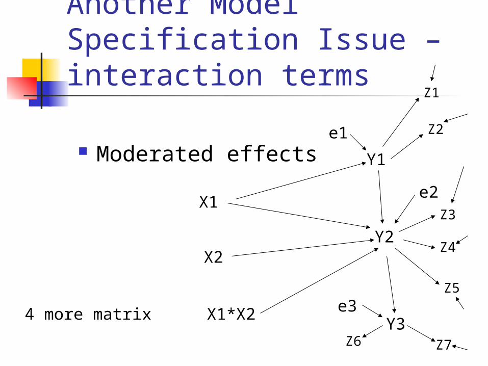
Another Model Specification Issue – interaction terms

Moderated effects

X1

X1*X2

X2Y2

Y1

Z1

Z2

Z5

Z4

Z3

4 more matrixY3

Z6 Z7

e1

e2

e3

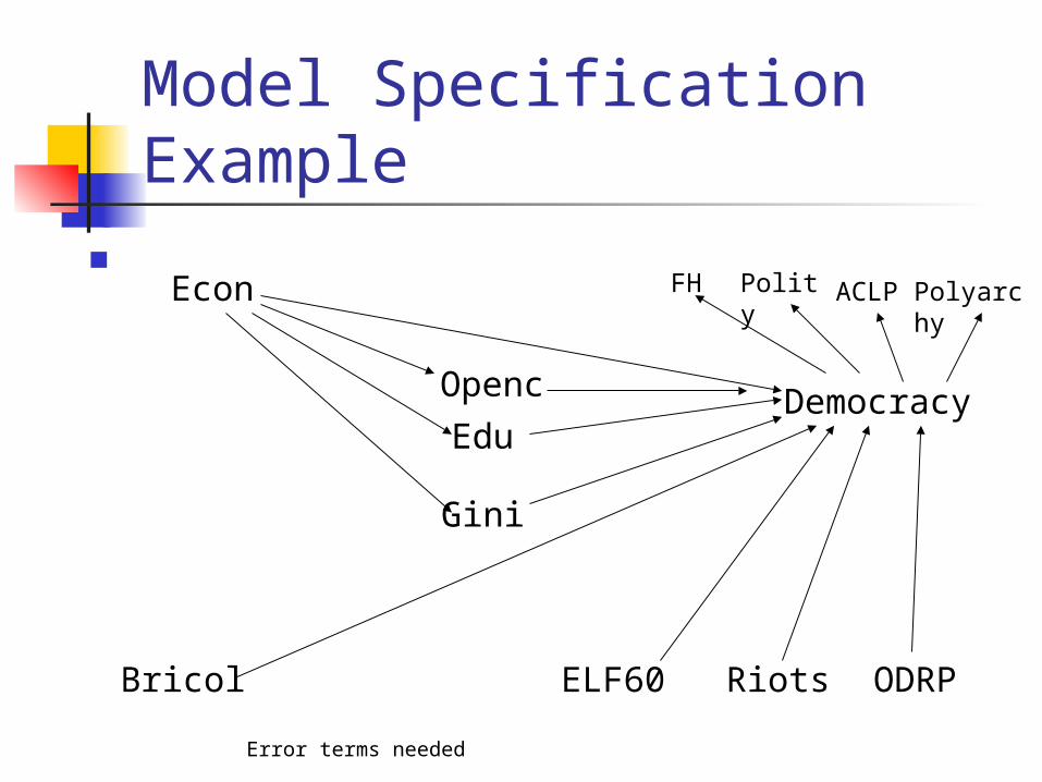
Model Specification Example

DemocracyEdu

Openc

Gini

Econ

ODRPRiotsELF60Bricol

FH Polity ACLP Polyarchy

Error terms needed

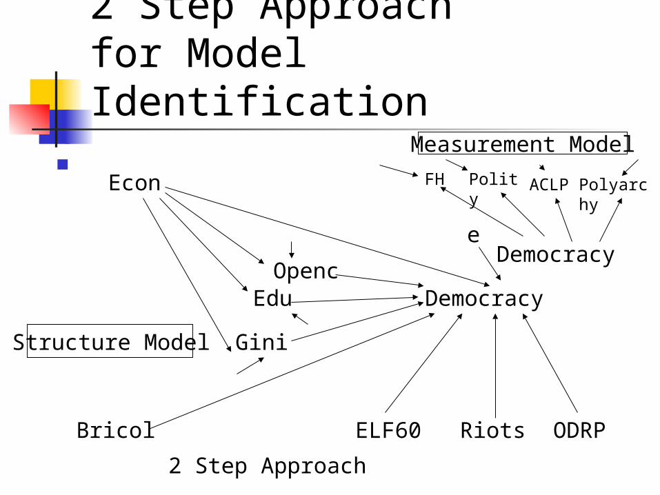
2 Step Approach for Model Identification

Democracy

Edu Openc

Gini

Econ

ODRPRiotsELF60Bricol

FH Polity ACLP Polyarchy

Democracy

Measurement Model

Structure Model

2 Step Approach

e

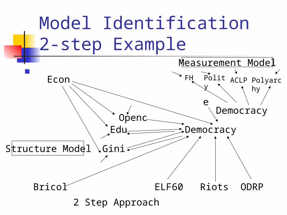
Model Identification 2-step Example

Democracy

Edu Openc

Gini

Econ

ODRPRiotsELF60Bricol

FH Polity ACLP Polyarchy

Democracy

Measurement Model

Structure Model

2 Step Approach

e

Data Preparation Missing Values Normality Multicollinearity Linearity

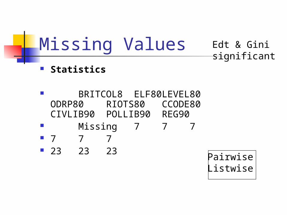
Missing Values Statistics

BRITCOL8 ELF80 LEVEL80ODRP80 RIOTS80 CCODE80CIVLIB90 POLLIB90 REG90

Missing 7 7 7 7 7 7 23 23 23

Edt & Ginisignificant

PairwiseListwise

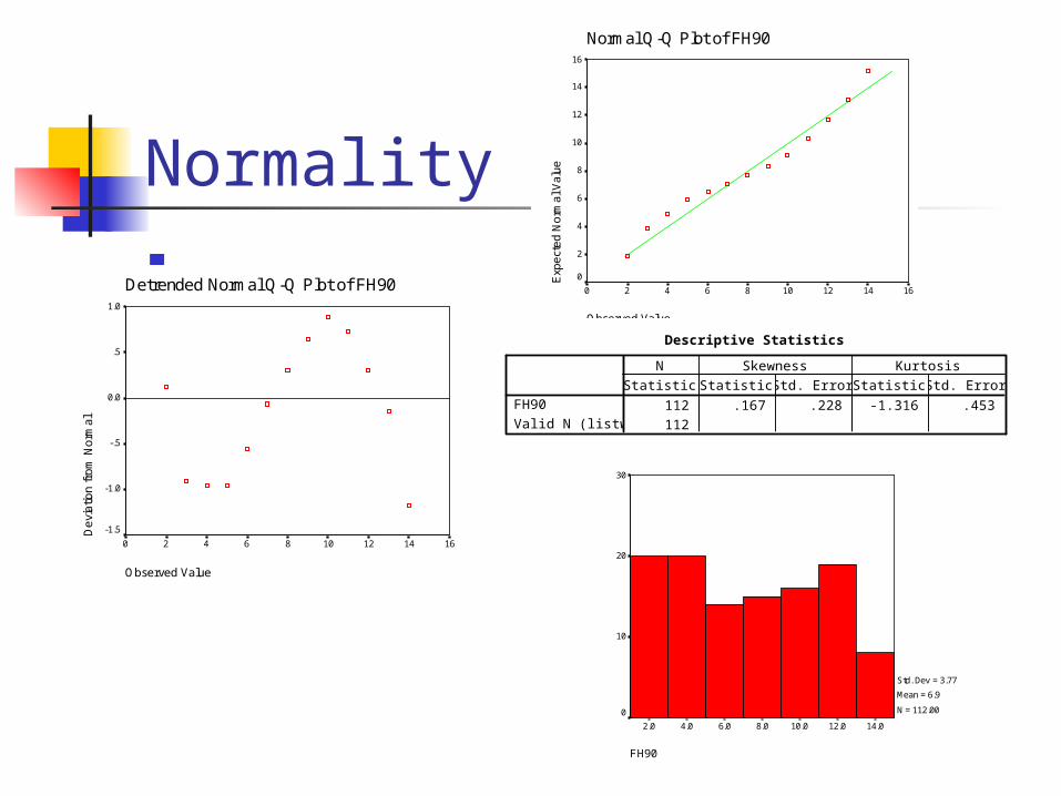
Normality

Normal Q-Q Plot of FH90

Observed Value

1614121086420

Exp

ect

ed

No

rma

l Va

lue

16

14

12

10

8

6

4

2

0Detrended Normal Q-Q Plot of FH90

Observed Value

1614121086420

De

via

tion

fro

m N

orm

al

1.0

.5

0.0

-.5

-1.0

-1.5

Descriptive Statistics

112 .167 .228 -1.316 .453

112

FH90

Valid N (listwise)

Statistic Statistic Std. Error Statistic Std. Error

N Skewness Kurtosis

FH90

14.012.010.08.06.04.02.0

30

20

10

0

Std. Dev = 3.77

Mean = 6.9

N = 112.00

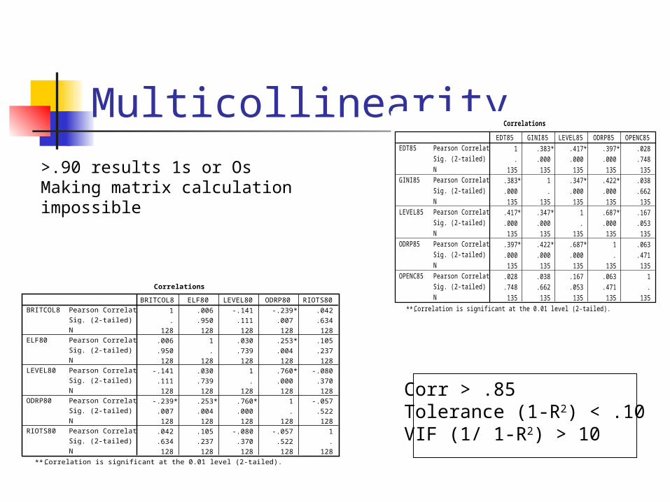
Multicollinearity

Correlations

1 .006 -.141 -.239** .042

. .950 .111 .007 .634

128 128 128 128 128

.006 1 .030 .253** .105

.950 . .739 .004 .237

128 128 128 128 128

-.141 .030 1 .760** -.080

.111 .739 . .000 .370

128 128 128 128 128

-.239** .253** .760** 1 -.057

.007 .004 .000 . .522

128 128 128 128 128

.042 .105 -.080 -.057 1

.634 .237 .370 .522 .

128 128 128 128 128

Pearson Correlation

Sig. (2-tailed)

N

Pearson Correlation

Sig. (2-tailed)

N

Pearson Correlation

Sig. (2-tailed)

N

Pearson Correlation

Sig. (2-tailed)

N

Pearson Correlation

Sig. (2-tailed)

N

BRITCOL8

ELF80

LEVEL80

ODRP80

RIOTS80

BRITCOL8 ELF80 LEVEL80 ODRP80 RIOTS80

Correlation is significant at the 0.01 level (2-tailed).**.

Correlations

1 .383** .417** .397** .028

. .000 .000 .000 .748

135 135 135 135 135

.383** 1 .347** .422** .038

.000 . .000 .000 .662

135 135 135 135 135

.417** .347** 1 .687** .167

.000 .000 . .000 .053

135 135 135 135 135

.397** .422** .687** 1 .063

.000 .000 .000 . .471

135 135 135 135 135

.028 .038 .167 .063 1

.748 .662 .053 .471 .

135 135 135 135 135

Pearson Correlation

Sig. (2-tailed)

N

Pearson Correlation

Sig. (2-tailed)

N

Pearson Correlation

Sig. (2-tailed)

N

Pearson Correlation

Sig. (2-tailed)

N

Pearson Correlation

Sig. (2-tailed)

N

EDT85

GINI85

LEVEL85

ODRP85

OPENC85

EDT85 GINI85 LEVEL85 ODRP85 OPENC85

Correlation is significant at the 0.01 level (2-tailed).**.

>.90 results 1s or Os Making matrix calculationimpossible

Corr > .85Tolerance (1-R2) < .10VIF (1/ 1-R2) > 10

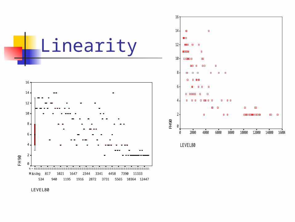
Linearity

LEVEL80

1600014000120001000080006000400020000

FH90

16

14

12

10

8

6

4

2

0

11111111111111111111111111111111111111111111111111111111111111111111111111111111111111111111111111111111116N =

LEVEL80

12447

11333

10364

7390

5565

4458

3731

3341

2872

2344

1916

1647

1195

1021

940

817

534

Missing

FH

90

16

14

12

10

8

6

4

2

0

Outliers outliers can distort the results

greatly

Variable Transformation

Power Function

Log For normality, linearity,

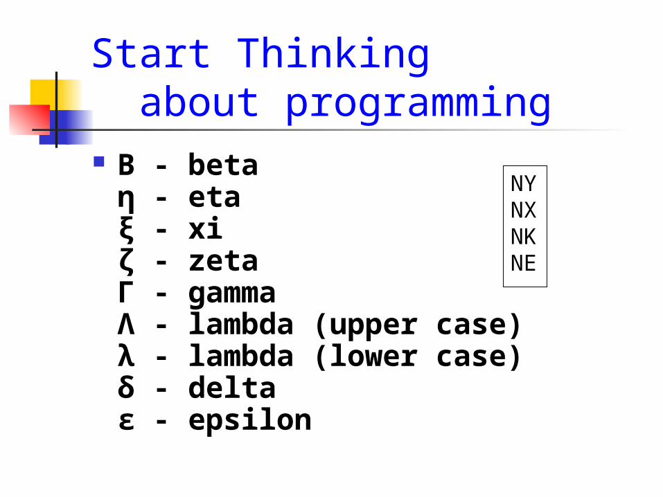
Start Thinking about programming Β - beta

η - etaξ - xiζ - zetaΓ - gammaΛ - lambda (upper case)λ - lambda (lower case)δ - deltaε - epsilon

NYNXNKNE

Introducing R R is FREE at www.r-project.org

R is very popular and powerful (see the NY Times article)

SEM in R example

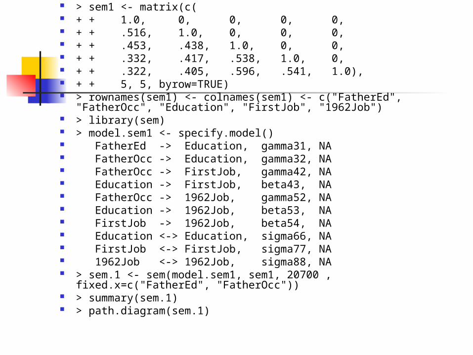
> sem1 <- matrix(c( + + 1.0, 0, 0, 0, 0, + + .516, 1.0, 0, 0, 0, + + .453, .438, 1.0, 0, 0, + + .332, .417, .538, 1.0, 0, + + .322, .405, .596, .541, 1.0), + + 5, 5, byrow=TRUE) > rownames(sem1) <- colnames(sem1) <- c("FatherEd", "FatherOcc",

"Education", "FirstJob", "1962Job") > library(sem) > model.sem1 <- specify.model() FatherEd -> Education, gamma31, NA FatherOcc -> Education, gamma32, NA FatherOcc -> FirstJob, gamma42, NA Education -> FirstJob, beta43, NA FatherOcc -> 1962Job, gamma52, NA Education -> 1962Job, beta53, NA FirstJob -> 1962Job, beta54, NA Education <-> Education, sigma66, NA FirstJob <-> FirstJob, sigma77, NA 1962Job <-> 1962Job, sigma88, NA > sem.1 <- sem(model.sem1, sem1, 20700 , fixed.x=c("FatherEd",

"FatherOcc")) > summary(sem.1) > path.diagram(sem.1)

About the Assignment Modify your hypotheses 1) Specify a few SEM models 2) Check their identification issues 3) Prepare your data

Write a 2 page report