structural control strategies for earthquake response reduction of
TRANSCRIPT

NSEL Report SeriesReport No. NSEL-043
August 2015
Department of Civil and Environmental EngineeringUniversity of Illinois at Urbana-Champaign
Takehiko Asai
and
Billie F. Spencer, Jr.
Structural Control Strategies for Earthquake Response Reduction of Buildings

UILU-ENG-2015-1809
ISSN: 1940-9826

The Newmark Structural Engineering Laboratory (NSEL) of the Department of Civil and
Environmental Engineering at the University of Illinois at Urbana-Champaign has a long history
of excellence in research and education that has contributed greatly to the state-of-the-art in civil
engineering. Completed in 1967 and extended in 1971, the structural testing area of the
laboratory has a versatile strong-floor/wall and a three-story clear height that can be used to carry
out a wide range of tests of building materials, models, and structural systems. The laboratory is
named for Dr. Nathan M. Newmark, an internationally known educator and engineer, who was
the Head of the Department of Civil Engineering at the University of Illinois [1956-73] and the
Chair of the Digital Computing Laboratory [1947-57]. He developed simple, yet powerful and
widely used, methods for analyzing complex structures and assemblages subjected to a variety of
static, dynamic, blast, and earthquake loadings. Dr. Newmark received numerous honors and
awards for his achievements, including the prestigious National Medal of Science awarded in
1968 by President Lyndon B. Johnson. He was also one of the founding members of the
National Academy of Engineering.
Contact:
Prof. B.F. Spencer, Jr.
Director, Newmark Structural Engineering Laboratory
2213 NCEL, MC-250
205 North Mathews Ave.
Urbana, IL 61801
Telephone (217) 333-8630
E-mail: [email protected]
This technical report is based on the first author’s doctoral dissertation of the same title, which
was completed in May 2014. The second author served as the dissertation advisor for this work.
Financial support for this research was provided in part by the Long Term Fellowship for Study
Abroad by the MEXT (Ministry of Education, Culture, Sports, Science, and Technology, Japan)
and the Newmark Account. Finally, we would like to thank the numerous collaborators on
this work, including Chia-Ming Chang and Brian Phillips.
The cover photographs are used with permission. The Trans-Alaska Pipeline photograph was
provided by Terra Galleria Photography (http://www.terragalleria.com/).

ABSTRACT
Destructive seismic events continue to demonstrate the importance of mitigating thesehazards to building structures. To protect buildings from such extreme dynamicevents, structural control has been considered one of the most effective strategies.
Structural control strategies can be divided into four classes: passive, active, semi-active, and hybrid control. Because passive control systems are well understood andrequire no external power source, they have been accepted widely by the engineeringcommunity. However, these passive systems have the limitation of not being able toadapt to varying conditions. While active systems are able to do that, they require asignificant amount of power to generate large control forces. Moreover, the stabilityof active systems is not ensured.
The focus of this report is the improvement and the validation of semi-activecontrol strategies, especially with MR dampers, for building protection from severeearthquakes. To make semi-active control strategies more practical, further studieson both the numerical and experimental aspects of the problem are conducted.
In the numerical studies, new algorithms for semi-active control are proposed.First, the nature of control forces produced by active control systems is investigated.The relationship between force-displacement hysteresis loops produced by the LQRand the LQG algorithms is explored. Then, new simple algorithms are proposed,which can produce versatile hysteresis loops. Moreover, the proposed algorithms donot require a model of the target structure to be implemented, which is a significantadvantage.
In the experimental studies, the effectiveness of semi-active control strategies areshown through real-time hybrid simulation (RTHS) in which a MR damper is testedphysically. In this report, smart outrigger damping systems for high-rise buildingsand smart base isolation systems are investigated. The accuracy of the RTHS em-ploying the model-based compensator for MDOF structures with a semi-active deviceis discussed as well.
The research presented in this report contributes the improvement and prevalenceof semi-active control strategies in building structures to mitigate seismic damage.

CONTENTS
Chapter 1 INTRODUCTION . . . . . . . . . . . . . . . . . . . . . . . 11.1 Motivation . . . . . . . . . . . . . . . . . . . . . . . . . . . . . . . . . 11.2 Semi-active control algorithms . . . . . . . . . . . . . . . . . . . . . . 21.3 Experimental verification of semi-active control strategies . . . . . . . 21.4 Overview . . . . . . . . . . . . . . . . . . . . . . . . . . . . . . . . . . 3
Chapter 2 LITERATURE REVIEW . . . . . . . . . . . . . . . . . . . 52.1 Structural control . . . . . . . . . . . . . . . . . . . . . . . . . . . . . 5
2.1.1 Outrigger damping system . . . . . . . . . . . . . . . . . . . . 82.1.2 Base isolation system . . . . . . . . . . . . . . . . . . . . . . . 8
2.2 Hysteresis loops produced by structural control force . . . . . . . . . 102.3 Semi-active control algorithms . . . . . . . . . . . . . . . . . . . . . . 112.4 Real-time hybrid simulation . . . . . . . . . . . . . . . . . . . . . . . 122.5 Summary . . . . . . . . . . . . . . . . . . . . . . . . . . . . . . . . . 13
Chapter 3 BACKGROUND . . . . . . . . . . . . . . . . . . . . . . . . 143.1 Modern control theory . . . . . . . . . . . . . . . . . . . . . . . . . . 14
3.1.1 LTI state space model . . . . . . . . . . . . . . . . . . . . . . 143.1.2 State feedback . . . . . . . . . . . . . . . . . . . . . . . . . . . 163.1.3 Observers . . . . . . . . . . . . . . . . . . . . . . . . . . . . . 163.1.4 Linear quadratic regulator (LQR) . . . . . . . . . . . . . . . . 183.1.5 Kalman filter . . . . . . . . . . . . . . . . . . . . . . . . . . . 183.1.6 Linear quadratic Gaussian (LQG) . . . . . . . . . . . . . . . . 19
3.2 Servo-hydraulic system model . . . . . . . . . . . . . . . . . . . . . . 203.2.1 Valve flow . . . . . . . . . . . . . . . . . . . . . . . . . . . . . 213.2.2 Actuator . . . . . . . . . . . . . . . . . . . . . . . . . . . . . . 223.2.3 Specimen . . . . . . . . . . . . . . . . . . . . . . . . . . . . . 223.2.4 Servo-controller . . . . . . . . . . . . . . . . . . . . . . . . . . 233.2.5 Servo-valve . . . . . . . . . . . . . . . . . . . . . . . . . . . . 233.2.6 Combined model . . . . . . . . . . . . . . . . . . . . . . . . . 24
3.3 Real-time hybrid simulation . . . . . . . . . . . . . . . . . . . . . . . 253.3.1 Types of delays . . . . . . . . . . . . . . . . . . . . . . . . . . 253.3.2 Experimental errors . . . . . . . . . . . . . . . . . . . . . . . . 26
3.4 Model-based compensators for RTHS . . . . . . . . . . . . . . . . . . 273.4.1 Feedforward compensator employing backward difference method 273.4.2 Bumpless feedforward compensator . . . . . . . . . . . . . . . 30

3.4.3 Feedforward-feedback compensator . . . . . . . . . . . . . . . 313.5 Summary . . . . . . . . . . . . . . . . . . . . . . . . . . . . . . . . . 34
Chapter 4 MODELING AND EXPERIMENTAL SETUP . . . . . . 354.1 MR damper modeling . . . . . . . . . . . . . . . . . . . . . . . . . . . 354.2 RTHS setup . . . . . . . . . . . . . . . . . . . . . . . . . . . . . . . . 374.3 Servo-hydraulic system modeling . . . . . . . . . . . . . . . . . . . . 404.4 Model-based compensator design for RTHS . . . . . . . . . . . . . . . 42
4.4.1 Bumpless feedforward compensator . . . . . . . . . . . . . . . 424.4.2 Feedforward-feedback compensator . . . . . . . . . . . . . . . 44
4.5 Summary . . . . . . . . . . . . . . . . . . . . . . . . . . . . . . . . . 46
Chapter 5 HYSTERESIS LOOPS PRODUCED BY ACTIVE CON-TROL FORCES . . . . . . . . . . . . . . . . . . . . . . . . . . . . . . 475.1 Active control in acceleration feedback: Problem formulation . . . . . 475.2 Hysteresis control force loops by numerical simulations . . . . . . . . 49
5.2.1 One-story building model . . . . . . . . . . . . . . . . . . . . 505.2.2 Three-story building model . . . . . . . . . . . . . . . . . . . 55
5.3 Summary . . . . . . . . . . . . . . . . . . . . . . . . . . . . . . . . . 63
Chapter 6 SEMI-ACTIVE CONTROL ALGORITHMS . . . . . . . 666.1 Problem formulation . . . . . . . . . . . . . . . . . . . . . . . . . . . 666.2 LQG-based clipped-optimal control . . . . . . . . . . . . . . . . . . . 676.3 Lyapunov stability-based control . . . . . . . . . . . . . . . . . . . . . 686.4 Model-free algorithms for semi-active control . . . . . . . . . . . . . . 69
6.4.1 Proposed simple algorithm 1 . . . . . . . . . . . . . . . . . . . 696.4.2 Proposed simple algorithm 2 . . . . . . . . . . . . . . . . . . . 69
6.5 Numerical simulation of the three-story building model . . . . . . . . 706.5.1 Building model . . . . . . . . . . . . . . . . . . . . . . . . . . 706.5.2 Controller design . . . . . . . . . . . . . . . . . . . . . . . . . 72
6.6 Results . . . . . . . . . . . . . . . . . . . . . . . . . . . . . . . . . . . 736.7 Summary . . . . . . . . . . . . . . . . . . . . . . . . . . . . . . . . . 87
Chapter 7 RTHS FOR SEMI-ACTIVE CONTROL ON A MDOFSTRUCTURE . . . . . . . . . . . . . . . . . . . . . . . . . . . . . . . 897.1 Smart outrigger damping system . . . . . . . . . . . . . . . . . . . . 89
7.1.1 Problem formulation . . . . . . . . . . . . . . . . . . . . . . . 897.1.2 Building model . . . . . . . . . . . . . . . . . . . . . . . . . . 917.1.3 Semi-active control designs . . . . . . . . . . . . . . . . . . . . 92
7.2 Results . . . . . . . . . . . . . . . . . . . . . . . . . . . . . . . . . . . 937.2.1 Influence of magnitude and time delay errors on RTHS . . . . 947.2.2 Experimental assessment . . . . . . . . . . . . . . . . . . . . . 95
7.3 Summary . . . . . . . . . . . . . . . . . . . . . . . . . . . . . . . . . 108
Chapter 8 VERIFICATION OF SMART BASE ISOLATION SYS-TEMS . . . . . . . . . . . . . . . . . . . . . . . . . . . . . . . . . . . . 1158.1 Base-isolated building model: Problem formulation . . . . . . . . . . 1158.2 Results . . . . . . . . . . . . . . . . . . . . . . . . . . . . . . . . . . . 117
8.2.1 Numerical simulation . . . . . . . . . . . . . . . . . . . . . . . 1178.2.2 RTHS . . . . . . . . . . . . . . . . . . . . . . . . . . . . . . . 137
8.3 Summary . . . . . . . . . . . . . . . . . . . . . . . . . . . . . . . . . 140
Chapter 9 CONCLUSIONS AND FUTURE STUDIES . . . . . . . 1439.1 Conclusions . . . . . . . . . . . . . . . . . . . . . . . . . . . . . . . . 1439.2 Future studies . . . . . . . . . . . . . . . . . . . . . . . . . . . . . . . 145
REFERENCES . . . . . . . . . . . . . . . . . . . . . . . . . . . . . . . . 147
Chapter 1
INTRODUCTION
1.1 Motivation
Severe earthquakes have caused serious damage to buildings all over the world, re-sulting in tremendous human suffering and great economic loss. Structural controlis one of the feasible options to enhance structural performance against such seismicevents (Housner et al., 1997). To date, various methods of structural control havebeen studied by many researchers and engineers, and some of them have been ap-plied successfully to real buildings. However, due to the stability, cost effectiveness,reliability, power requirements, etc., structural control strategies have yet to be fullyaccepted by the building engineering community.
Structural control systems can be placed into four basic categories: passive, ac-tive, semi-active, and hybrid. Passive systems, including base isolation, viscoelasticdampers, and tuned mass dampers, are well understood and are accepted widely bythe engineering community as a means for mitigating the effect of strong earthquakes.However, these passive device methods have the limitation of not being able to adaptto structural change and to varying usage patterns and loading conditions. Whileactive systems have the ability to adapt to various operating conditions, they requirelarge power sources to impart forces to the structure, and may fail during seismicevents. Another concern of active systems is that the stability of the system is notguaranteed.
Semi-active control devices have received a great deal of attention in recent yearsas a means to address drawbacks of passive and active systems. They offer the adapt-ability to structural changes and to various usage patterns and loading conditions,and they do not require large power sources to control devices. In fact, many can op-erate on battery power, which is critical during seismic events. Moreover, in contrastto active control systems, semi-active control systems do not have the potential todestabilize the structural system (in the bounded input/bounded output sense).
One of the promising devices for semi-active control systems is the magnetorheo-logical (MR) damper (Carlson and Spencer, 1996), which is filled with magnetorhe-ological fluid and controlled by a magnetic field. This magnetic field allows thedamping characteristics to be continuously controlled by varying the input ampli-tude. The advantage of MR dampers is that they contain no moving parts other thanthe piston, which makes them very reliable. Moreover, MR fluid is not sensitive toimpurities such as are commonly encountered during manufacturing and usage, andlittle particle/carrier fluid separation takes place in modern MR fluid under commonflow conditions. So the future of application of MR dampers into civil structuresappears to be quite bright. Nonetheless, to make semi-active systems employing MR
1
dampers more implementable, further studies are still needed.
1.2 Semi-active control algorithms
Developing more effective semi-active control algorithms is an important step towardpractical use. Although various semi-active control algorithms have been proposed,applying these algorithms in real civil structures needs a relatively accurate model ofthe structure. However, obtaining accurate parameter values for full-scale structuresmay not be practical. And the structure may change with time, resulting in theneed to continuously update the model. Thus, developing effective simple algorithmswhich do not require the structural model or a large number of sensors is desirablefor practical use.
Moreover, to ensure appropriate seismic performance of structures, the earth-quake input energy absorption capability of control devices described by hysteresisloops plays a key role. However, in semi-active control, because only the propertiesof the devices are controlled, the nature of desired hysteresis loops is difficult to as-certain. For example, MR dampers, for which only input current can be controlled,cannot produce force such that the force and velocity have the same direction. There-fore, semi-active control algorithms which can realize specific hysteresis loops are alsodesirable in the field of seismic response control.
Thus, proposing model-free algorithms which can realize a variety of control forceproperties is demanded in the field of semi-active control.
1.3 Experimental verification of semi-active
control strategies
Second, experimental verification for semi-actively controlled structures is necessary.However, experimental studies at large scale have been limited. Because creatingthe mathematical model of a MR damper is challenging due to its highly nonlin-ear response, physical experiments are vital to verify the effectiveness of semi-activemethods employing MR dampers. Although shaking table testing provides a directapproach to evaluate the dynamic structural response of civil structures subjected toearthquake loads, even if large facilities such as the E-Defense table in Japan or theshaking table at the University of California at San Diego are available, tests for largecivil structures such as high-rise buildings are impractical due to limitations on thesize, payload capacity, and cost.
Hybrid simulation is a powerful, cost-effective method for testing structural sys-tems. Through substructuring, the well-understood components of the structure aremodeled numerically, while the components of interest are tested physically. Then,by coupling numerical simulation and experimental testing, the complete responseof a structure is obtained. When the rate-dependent behavior of the physical spec-imen is important (e.g., MR damper), real-time hybrid simulation (RTHS) must beemployed. In RTHS, computation, communication, and actuator limitations cause
2
delays and lags which lead to inaccuracies and potential instabilities. The highermodes are affected more by these effects, reducing accuracy of the simulation, poten-tially leading to instability of the RTHS. Thus, research on RTHS has been limitedto simple structures; e.g., SDOF and 2DOF.
To compensate for these time delays and lags, as well as control-structure interac-tion (CSI) between the actuator and the specimen (Dyke et al., 1995), model-basedactuator-control approaches have been proposed (Carrion and Spencer, 2007; Phillipsand Spencer, 2012). However, applications of this method to MDOF structures, whichinclude high frequency components, are still limited. To show the effectiveness of themodel-based compensator for RTHS, further studies on MDOF structures should beimplemented.
One of the structural control methods to show its effectiveness is smart outriggerdamping systems employing semi-actively controlled MR dampers. The effectivenessof this method has been verified through numerical simulations (Chang et al., 2013),however experimental validations have not conducted yet.
Smart base isolation systems are another class of structural control systems thatneed further experimental validation. They are composed of a base isolation systemcombined with semi-actively controlled MR dampers. Passive base isolation is onecommon type of structural control system, increasing the structure’s flexibility tomitigate the effect of potentially dangerous seismic ground motions. However, largebase displacements resulting from the increased flexibility of the passive isolationsystem can potentially exceed the allowable limit of structural designs under severeseismic excitations. Smart base isolation systems are a potential alternative meansto address the drawbacks of passive and active isolation systems.
1.4 Overview
This report focuses on the development and experimental verification of semi-activecontrol strategies for earthquake response reduction of buildings. To show that semi-active control is a structural control strategy comparable to active control or evenbetter in a sense, theoretical and experimental studies are conducted. This sectionprovides a description of the contents of each chapter of this report.
Chapter 2 contains a detailed review of the previous studies related to this report.First of all, various types of structural control strategies, especially outrigger dampingand base isolation systems, are reviewed. Second, literature about hysteresis loopsproduced by structural control forces are introduced. Third, studies on RTHS witha focus on compensators are summarized. The issues and difficulties to overcome areaddressed briefly, as well.
Chapter 3 provides technical background necessary for this report that mightbe unfamiliar to researchers and engineers in civil engineering. The basics of moderncontrol theory focusing on linear quadratic regulator (LQR), Kalman filter, and linearquadratic Gaussian (LQG) control theories are presented. Also, a servo-hydraulicmodel used in this report is presented. Two types of model-based compensatorsfor the dynamics of the servo-hydraulic system, such as bumpless feedforward and
3

feedforward-feedback compensation, are developed as well.Chapter 4 builds the MR damper model used for numerical simulation and de-
scribes the experimental setup for RTHS. The servo-hydraulic model is created andthe two model-based compensators discussed in Chapter 3 are designed for RTHS, aswell.
Chapter 5 investigates the nature of the hysteresis loops produced by active controlforces. The behavior of the hysteresis force-displacement loops produced by the LQRfull-state feedback and the LQG-based acceleration feedback strategies is consideredthrough numerical simulation studies on scaled one-story and three-story buildings.By comparing the results obtained from these two algorithms, the accuracy of theacceleration feedback is explored as well.
Chapter 6 describes algorithms for semi-active control strategies. First, the LQG-based clipped-optimal control, one of the widely accepted algorithms, is reviewedbriefly. Then, new simple algorithms are presented, which do not require a structuremodel and enable versatile control force properties. Subsequently, hysteresis loops andseismic performance produced by these algorithms are compared through numericalsimulation on a scaled three-story building model.
Chapter 7 verifies the effectiveness of the model-based RTHS compensator for asemi-actively controlled MR damper installed in a MDOF structure. For the MDOFstructure, a high-rise building model with an outrigger damping system is employedwhich is analyzed numerically, while the MR damper is tested physically. The effectof the compensation errors in RTHS is examined. Also, seismic performance of thesmart outrigger damping system employing MR dampers is explored.
Chapter 8 extends the application of the semi-active control framework into hybridbase isolation systems. The six-story base isolation building model in the SmartStructures Technology Laboratory (SSTL) at the University of Illinois at Urbana-Champaign is employed to verify the effectiveness of the smart base isolation system,in which MR dampers are installed to a passive base isolation system; this is shownthrough numerical simulation and RTHS. Finally, the seismic performance is discussedby comparing it with the active base isolation case.
Chapter 9 summarizes the research presented in this report and provides recom-mendations and possible directions for future work on structural control technologiesfor seismic protection of buildings.
4

Chapter 2
LITERATURE REVIEW
This chapter provides a literature review of various types of structural control methodsfocusing on outrigger damping and base isolation systems. A brief review of thebehavior of the force-displacement hysteresis loops produced by structural controlstrategies, as well as RTHS techniques, is also included.
2.1 Structural control
The purpose of the structural control in civil structures is to reduce structural vibra-tion produced by external forces, such as earthquake and wind, by various means suchas modifying stiffness, mass, damping, or shape. Structural control systems employedin civil engineering fall into four basic categories, i.e., passive, active, semi-active, andhybrid control. This section describes various structural control methods in each cate-gory studied by many researchers to this date, focusing on outrigger damping systemsand base isolation systems.
Passive systems employ supplemental devices, which respond to the motion ofthe structure, to dissipate vibratory energy triggered by strong earthquakes and highwinds in the structural system without external power sources. These systems aresimple to understand and are accepted by the engineering community as a means formitigating the effects of severe dynamic loadings. A variety of passive control mech-anisms have been suggested by many researchers and engineers, including metallicyield dampers (Whittaker et al., 1991), viscous dampers (Constantinou et al., 1993;Reinhorn et al., 1995), tuned mass damper (Den Hartog, 1956; Villaverde, 1994), andbase isolation (Kelly et al., 1987; Kelly, 1997). However, because these passive de-vices cannot adapt to structural changes and to varying usage patterns and loadingconditions, there exist limitations.
Active control systems operate by using external energy supplied by actuators toimpart forces on the structure. The appropriate control action is determined basedon measurements of the structural responses. The concept of the strategy in civilstructures was first suggested by Yao (1972). Yang (1975) applied modern controltheory to control the vibration of civil engineering structures under random loadings.Active control techniques are generally able to achieve higher control performance,as compared to passive control techniques (Soong and Costantinou, 1995).
The first full-scale application of an actively controlled building, the KyobashiCenter building (Figure 2.1), was achieved in 1989 in Japan by the Kajima Corpora-tion (Kobori, 1990, 1996). Subsequently, active control strategies have been appliedto many buildings and bridges, particularly in Asia. To date, many studies related toactive control methods have been performed, and significant progress has been made
5

Figure 2.1: Kyobashi Center building with AMD installation
toward protecting civil structures from severe environmental loads using these ad-vances including the active bracing system (Reinhorn et al., 1989), the active tunedmass damper/driver (Abdel-Rohman and Leipholz, 1983; Chang and Soong, 1980)and the active aerodynamic appendage mechanism (Soong and Skinner, 1981; Abdel-Rohman, 1984).
Various control algorithms for active systems have been considered. Output feed-back strategies using absolute acceleration measurements were developed by Spenceret al. (1994); Suhardjo et al. (1992). Control algorithms which account for the forceand stroke limitations of control actuators have been investigated (Tamura et al.,1994). Nonlinear control algorithms have also been considered in an effort to increasethe effectiveness of these active systems (Gattulli et al., 1994). Other types of controlalgorithms that have been suggested for active control systems include fuzzy control(Chameau et al., 1991; Furuta et al., 1994), neural-based control (Casciati et al., 1993;Shoureshi et al., 1994), and sliding mode control (Yang et al., 1994).
Although many successful experiments and implementations proved the activecontrol technology as a practical technique, some potential risks still exist in theirreal-time implementation; for example, the external energy injected by the active con-trol devices might destabilize the system if the measurements of structural responseshave been perturbed, the control laws are developed from a system model that mis-represents the true behavior of systems, the interaction between the structure and thecontrol devices has been exclusively considered in the development of control laws,and so on. These details involved in the structural implementation of active controltechniques continue to be an area of research interest.
Semi-active control devices have received a great deal of attention in recent yearsbecause they offer the adaptability of active control devices without requiring theassociated large power sources. In fact, many can operate on battery power, which iscritical during seismic events when the main power source to the structure may fail.According to presently accepted definitions, a semi-active control device is one that
6
cannot increase the mechanical energy in the controlled system (i.e., including boththe structure and the device), but has properties which can be dynamically varied tooptimally reduce the responses of a structural system. Therefore, in contrast to activecontrol devices, semi-active control devices do not have the potential to destabilizethe structural system (in the bounded input/bounded output sense). Preliminarystudies indicate that appropriately implemented semi-active systems perform signifi-cantly better than passive devices and have the potential to achieve, or even surpass,the performance of fully active systems, thus allowing for the possibility of effectiveresponse reduction during a wide array of dynamic loading conditions.
To date, various semi-active devices have been proposed. Variable-orifice dampersto control the motion of bridges experiencing seismic motion was first discussed byFeng and Shinozuka (1990). Variable damping is achieved by altering the resistanceto flow of a conventional hydraulic fluid. Akbay and Aktan (1990, 1991) and Kannanet al. (1995) proposed variable friction devices which consists of a friction shaft whichis rigidly connected to the structural bracing. The force at the frictional interfacewas adjusted to allow controlled slippage. Lou et al. (1994) proposed a semi-activedevice based on a passive tuned sloshing damper (TSD), in which the length of thesloshing tank could be altered to change the properties of the device. Haroun et al.(1994) presented a semi-active device based on a tuned liquid column damper (TLCD)with a variable-orifice. Controllable fluids such as electrorheological (ER) fluids andmagnetorheological (MR) fluids were discovered in the late 1940s (Winslow, 1947,1949; Rabinow, 1948). Prior to MR fluid dampers, a number of ER fluid damperswere developed, modeled, and tested for civil engineering applications (Ehrgott andMasri, 1994; Gavin et al., 1994a,b; Gordaninejad et al., 1994; Makris et al., 1995,1996; McClamroch and Gavin, 1995). The recently developed MR fluids appear to bean attractive alternative to ER fluids for use in controllable fluid dampers (Carlson,1994; Carlson and Weiss, 1994; Carlson et al., 1996; Spencer et al., 1997; Dyke et al.,1996c).
Because all of these semi-active devices are intrinsically nonlinear, one of themain challenges is to develop control strategies that can optimally reduce structuralresponses. Various nonlinear control strategies have been developed to take advantageof the particular characteristics of the semi-active devices, including bang-bang con-trol (McClamroch and Gavin, 1995), clipped-optimal control (Patten et al., 1994a,b;Dyke et al., 1996c), bistate control (Patten et al., 1994a,b), fuzzy control meth-ods (Sun and Goto, 1994), and adaptive nonlinear control (Kamagata and Kobori,1994), pseudo-negative stiffness algorithm (Iemura and Pradono, 2002, 2005), Lya-punov based control (Jansen and Dyke, 2000; Wang and Gordaninejad, 2002), slidingmodel control (Luo et al., 2000; Moon et al., 2003), backstepping control (Ikhouaneet al., 1997; Luo et al., 2006), quantitative feedback theory (Zapateiro et al., 2008),and mixed H2/H∞ control (Yang et al., 2003, 2004b; Karimi et al., 2009).
Hybrid control strategies have been investigated by many researchers to exploittheir potential to increase the overall reliability and efficiency of the controlled struc-ture (Soong and Reinhorn, 1993). A hybrid control system is typically defined as onewhich employs a combination of two or more passive, active, or semi-active devices.Because multiple control devices are operating, hybrid control systems can alleviate
7
some of the restrictions and limitations that exist when each system is acting alone.Thus, higher levels of performance may be achievable.
The hybrid mass damper (HMD) is the most common control device employedin full-scale civil engineering applications. The HMD is a combination of a tunedmass damper (TMD) and an active control actuator. Tanida et al. (1991) developedan arch-shaped HMD that has been employed in a variety of applications, includingbridge tower construction, building response reduction and ship roll stabilization.Another class of hybrid control systems which has been investigated by a numberof researchers is found in the active or semi-active base isolation system (Inaudyand Kelly, 1990; Spencer et al., 2000), consisting of a passive base isolation systemcombined with actuators or semi-active devices to supplement the effects of the baseisolation system. The details of these systems are discussed in the section 2.1.2.
2.1.1 Outrigger damping system
The number of high-rise buildings in urban areas around the world has dramaticallyincreased in the past two decades, spurred by the development of new materials andtechnologies. However, this achievement also generates new problems; specifically,how these buildings can be protected from strong winds and severe earthquakes.To protect these tall buildings from such severe loadings, researchers and engineershave considered various passive structural control strategies, such as viscous dampers,viscoelastic dampers, and tuned mass dampers (Kareem et al., 1999; Spencer andNagarajaiah, 2003). However, interstory drifts of a size that is sufficient to dissipatelarge amounts of input energy are generally not available in high-rise buildings. Tosolve this problem, numerous response amplification systems have been proposed, e.g.toggle braces (Constantinou et al., 2001), scissor-jacks (Sigaher and Constantinou,2003), gear-type systems (Berton and Bolander, 2005), and the mega brace (Taylor,2003).
Smith and Salim (1981); Charles (2006); Smith and Willford (2007) have proposedoutrigger damping systems as an alternative response amplification method. This sys-tem employs vertical viscous dampers installed between outrigger walls and perimetercolumns in a frame-core-tube structure to enhance structural dynamic performance.Willford et al. (2008) reported on a real-world implementation in a high-rise buildingin the Philippines. While successful, this approach is a passive system, which is un-able to adapt to structural changes, varying usage patterns, and loading conditions.In the outrigger damping system, Wang et al. (2010) and Chang et al. (2013) pre-sented numerical examples of semi-actively controlled outrigger systems employingMR dampers, achieving superior performance over the corresponding passive system.
2.1.2 Base isolation system
A base isolation system falls into passive systems. The concept of seismic base iso-lation is to isolate the structure and its contents from potentially dangerous groundmotion, especially within the frequency range where the building is most affected by
8

inserting low stiffness devices such as lead-rubber bearings, friction-pendulum bear-ings, or high damping rubber bearings between the structure and ground. The goalis to reduce interstory drifts and absolute accelerations to avoid damage by absorbingearthquake energy with these devices. However, the unacceptable base displacementresponses in passive base isolation systems have been reported. Thus, the extra damp-ing devices and controllable devices are encouraged to reduce the base displacements.
To achieve this demand, active base isolation, where a passive isolation systemcombined with active control devices, such as hydraulic actuators, has been proposed.The combination shares the advantages of the reductions in passive isolation systems,i.e., absolute floor accelerations, interstory drifts, and base shears, as well as thereductions in base displacements from the contributions of the actuators (Inaudy andKelly, 1990).
Many numerical studies were conducted by applying different control algorithmssuch as the classic linear quadratic regulation (LQR) control algorithm and the Lya-punov control algorithm (Inaudy and Kelly, 1990; Pu and Kelly, 1991; Loh and Chao,1996; Yang et al., 1992; Loh and Ma, 1996; Fur et al., 1996). Different active controldevices, such as active tuned mass dampers or active vibration absorbers (differentfrom hydraulic actuators), were also considered (Loh and Chao, 1996; Lee-Glauseret al., 1997). Some researchers focused on the numerical analysis of different isolationbearings, such as rubber bearings or sliding bearings (Yang et al., 1995; Feng, 1993).
The effectiveness of active base isolation systems was verified experimentally aswell. Yang et al. (1996) employed the sliding mode control algorithm to control a slid-ing base-isolated, three-story building through shake table testing. Riley et al. (1998)developed a nonlinear controller to experimentally implement a hydraulic actuatorfor controlling a three-story, base-isolated building. Nishimura and Kojima (1998)considered a building-like structure incorporated with an isolator and an actuatorfor verification of active base isolation. Although these experiments only consideredthe in-plane motions of structures under unidirectional excitations, these providedevidence of the applicability and feasibility of active base isolation systems. Changand Spencer (2012) developed active isolation strategies for multi-story buildings sub-jected to bi-directional earthquake loadings and verified the efficacy experimentally.
Smart base isolation is another class of hybrid base isolation system (Spencer et al.,2000; Yoshioka et al., 2002). Smart base isolation is composed of a passive base iso-lation system combined with control structures with semi-active control devices, e.g.,variable orifice dampers (Wongprasert and Symans, 2005); semi-active independentlyvariable dampers (SAIVD) (Nagarajaiah and Narasimhan, 2007), electrorheologicaldampers (Makris, 1997); and magnetorheological (MR) dampers (Ramallo et al.,1999, 2002; Nagarajaiah and Narasimhan, 2006; Narasimhan et al., 2008; Wang andDyke, 2013). This combination shares the advantages of semi-active control such asadaptivity to excitations, low-power requirements, and stability, while still performingcomparably to actively controlled isolation systems.
Many numerical studies of smart base isolation systems employing MR dampershave been investigated. Ramallo et al. (2002) studied an isolated building with lam-inated rubber bearings. The results demonstrated acceptable control performance inthe reductions of the accelerations and displacements. Nagarajaiah and Narasimhan
9
(2006) shows the effectiveness of a three-dimensional smart base-isolated building withlinear and frictional isolation system. Narasimhan et al. (2008) considered the nonlin-earities in lead-rubber-bearing (LRB). Chang et al. (2008) applied a scheduled controlstrategy to a nonlinear control problem of a smart base-isolated building. Wang andDyke (2013) presented the advantages of applying a modal linear quadratic Gaussian(LQG) approach for base isolation systems. These numerical studies have demon-strated the applicability of smart base isolation systems employing MR dampers.
To show the efficacy of smart base isolation systems employing MR dampers,some experimental studies using a shaking table have been conducted. Yoshioka et al.(2002) verified a smart base isolation system employing laminated rubber bearings ofa single-story small-scale building. Sahasrabudhe and Nagarajaiah (2005) applied theLyapunov-based control algorithm to a scaled two-story smart base isolation system.Lin et al. (2007) employed fuzzy logic control by applying smart base isolation withfour high damping rubber bearings and a 300 kN MR damper. Moreover, Shooket al. (2007) considered a single-story building installed with bi-directional slidingbearings and planar MR dampers (e.g., MR dampers were placed in two directions)under bi-directional excitations. In these studies, most structures are scaled and maymisrepresent the performance of controlled structures.
These results proved that the combination of this smart base isolation system caneffectively reduce the base displacements as well as interstory drifts. These numericalstudies have demonstrated the applicability of semi-active base isolation systems,although a simulation might not sufficiently represent the true control performancein a practical implementation. Therefore, the experimental studies of these systemsare needed. Also, since most numerical studies were investigated under unidirectionalexcitations, the efficacy of multi-axial semi-active base isolation should be shown.
2.2 Hysteresis loops produced by structural
control force
In the field of earthquake engineering, energy absorbing-devices are added to struc-tures to dissipate input energy effectively. The input energy absorption capabilityof these devices plays a key role in mitigating earthquake damage. Therefore, 1)elucidating the relationship between the property of control forces and the structuralresponses and 2) developing structural control devices and appropriate algorithms forthem which enable intended control forces are desirable.
The effectiveness of negative stiffness was found in skyhook control proposed byKarnopp et al. (1974). In the ideal condition of the skyhook system, a structure isconnected to a virtual fixed point in the sky through a dashpot. In practical use, theskyhook damper is realized by active or semi-active controllers.
The negative stiffness produced by active control force using linear quadratic regu-lator (LQR) was investigated by Iemura and Pradono (2005) on a cable-stayed bridgemodel. They showed that the LQR control algorithm produced hysteresis loops withnegative stiffness and reduced the displacements and base shear to earthquake exci-
10

tations.Iemura and Pradono (2009) showed that the semi-actively controlled skyhook
damper produces a damping force proportional to the absolute velocity of the mass,and negative stiffness appears in the hysteresis loops. Iemura and Pradono (2002,2005) proposed an algorithm for semi-actively controlled viscous dampers to producenegative stiffness and showed the seismic performance on a cable-stayed bridge. Thepossibility of producing negative stiffness by MR dampers were shown in Iemura et al.(2006); Weber and Boston (2011); Wu et al. (2013) as well.
Recently, passive methods to produce negative stiffness damping have been re-ported as well. Negative stiffness friction damper is proposed by Iemura and Pradono(2009); Iemura et al. (2008, 2010), which is quite similar to an ordinary friction pendu-lum support, but the inverted curve is introduced. Since the vertical weight inducedon the unstable convex slide plate accelerates the horizontal deformation due to thegravitational effect, the force is negatively proportional to the deformation. Thedynamic behavior of the proposed negative stiffness damper was assessed by usingthe large-scale shaking table at the Disaster Prevention Research Institute (DPRI)of Kyoto University, Japan. An adaptive negative stiffness device is proposed anddeveloped by Nagarajaiah et al. (2010). In this device, adaptive negative stiffnessbehavior is realized by possessing predesigned variations of stiffness as a function ofstructural displacement amplitude. The effectiveness of the proposed mechanism inelastic and inelastic structural systems was demonstrated through simulation for peri-odic and random input ground motions. Viti et al. (2006) produced negative stiffnesspassively through a new retrofitting procedure which weakened the strength of thestructure and added supplemental damping devices. The proposed method reducedboth accelerations and ductility demand on a five-story hospital building.
2.3 Semi-active control algorithms
Semi-active control has been proposed as an alternative method for active control(Housner et al., 1997). Like active control, semi-active control offers the adaptabilityto structural changes and to various usage patterns and loading conditions. More-over, semi-active control devices such as the variable-orifice damper, variable-frictiondamper, electrorheological (ER) damper, and magnetorheological (MR) damper re-quire little power, because the energy is used to modify only the device’s properties(e.g., stiffness and damping). The effectiveness of semi-active control has been shownthrough numerous numerical simulations and experiments (Dyke et al., 1996d,c;Spencer et al., 1997; McClamroch et al., 1994; McClamroch and Gavin, 1995; Leit-mann, 1994; Jansen and Dyke, 2000; Wang and Gordaninejad, 2002; Luo et al., 2000,2003; Moon et al., 2003; Ikhouane et al., 1997; Zapateiro et al., 2009; Luo et al., 2004;Zapateiro et al., 2008).
Various algorithms have been proposed for semi-active control devices to miti-gate seismic damage; e.g., linear quadratic Gaussian (LQG)-based clipped-optimalcontrol (Dyke et al., 1996d,c; Spencer et al., 1997), bang-bang control McClamrochet al. (1994); McClamroch and Gavin (1995), control based on Lyapunov stability
11

Figure 2.2: E-Defense, Miki, Hyogo, Japan
theory (Leitmann, 1994; Jansen and Dyke, 2000; Wang and Gordaninejad, 2002),sliding mode control (Luo et al., 2000, 2003; Moon et al., 2003), backstepping con-trol (Ikhouane et al., 1997; Zapateiro et al., 2009), and quantitative feedback theory(QFT) (Luo et al., 2004; Zapateiro et al., 2008). To apply these algorithms for realcivil structures, a relatively accurate model is needed. However, obtaining accurateparameter values for full-scale structures may not be practical. Moreover, the struc-ture may change with time, resulting in the need to continuously update the model.Thus, developing effective simple algorithms which do not require the structural modelor a large number of sensors is desirable for practical use.
2.4 Real-time hybrid simulation
Shaking table testing provides a direct approach to evaluate the dynamic structuralresponse of civil structures subjected to earthquake loads. However, shaking tablestudies at large scale have been limited so far. This is because, even if large facilitiessuch as the E-Defense table in Japan (Figure 2.2) or the shaking table at the Uni-versity of California at San Diego are available, tests for large civil structures such ashigh-rise buildings are impractical due to limitations on the size, payload capacity,and cost.
As an alternative method, hybrid simulation was first proposed by Hakuno et al.(1969) to test a single degree of freedom model subjected to seismic loads. Theequations of motion were solved using an analog computer while an electromagneticactuator was used to excites the physical specimen in real-time. Hardware limita-tions also compromised the accuracy of the experiment by adding a phase lag thatwas recognized but uncompensated. Hybrid simulation was established in its cur-rent recognizable form through the introduction of discrete time systems and digitalcontrollers (Takanashi et al., 1974, 1975). Employing a digital controller to solve
12
the equations of motion, the real-time loading constraint could be relaxed to a rampand hold procedure over an extended time scale. Typical quasi-static testing equip-ment could be used while numerical integration could be performed at a slower rateappropriate for the computers.
As rate-dependent structural control devices such as base isolation bearings andfluid dampers have been developed, the demand of expanding hybrid simulationto include a more rigorously verified real-time framework has been increased. Thefirst modern real-time hybrid simulation using digital computers was conducted byNakashima et al. (1992) on a SDOF system. In this study, a digital servo-mechanismbetween the computer performing the numerical integration and the servo-controllerwas introduced to seek accurate velocity control. This digital servomechanism oper-ated as a ramp generator between numerical integration time steps and also includeda feedback loop to improve the displacement performance at substeps of the numericalintegration.
Horiuchi et al. (1996) studied the effect of time delay on RTHS in detail andproposed the polynomial extrapolation delay compensation scheme. In this study, asuper real-time controller (Umekita et al., 1995) using parallel computing and a specialprogramming language was employed to calculate the equations motions within therequired time step. Separating the tasks of signal generation and response analysiswas proposed by Nakashima and Masaoka (1999), allowing RTHS to be performed oncommercially available processors. Many studies have been reported to enhance theperformance of RTHS since these pioneering studies.
Carrion and Spencer (2007) presented another approach for time delay/lag com-pensation using model-based response prediction. Verification experiments showedthat model-based compensation allowed testing systems with natural frequencies ashigh as 13 Hz for linear response and 15 Hz for inelastic response. Experimentalresults using a structure with the MR damper verified that the approach and test-ing system presented were capable of testing rate-dependent devices. Phillips andSpencer (2012) improved the model-based actuator control by combining a feedbackcontroller with a feedforward controller. The effectiveness of the proposed methodwas shown on a single-actuator system and multi-actuator system.
2.5 Summary
The references on the development of various types of structural control strategiesto reduce damage on buildings from earthquakes are provided in this chapter. Thischapter reviews the literature on hysteresis loops produced by control forces andRTHS method to verify the efficacies of these methods as well. Huge efforts have beenmade by many researchers and engineers to improve structural control technologies inbuildings. However, further development is still required to realize their full potential.
13
Chapter 3
BACKGROUND
Some background in modern control theory is provided in this chapter to lay thegroundwork for subsequent active and semi-active controller designs. A linearizedmodel of the servo-hydraulic actuator system, time delays and lags of real-time hybridsimulation (RTHS), and model-based compensations for RTHS are also described inthis chapter.
3.1 Modern control theory
Whereas classical control theory focuses on frequency domain analysis employingtransfer function approaches, modern control theory is based on time domain analy-sis expressed by first-order differential equations utilizing state space representation.This section presents necessary basic knowledge on liner time-invariant system (LTI)to understand this report.
3.1.1 LTI state space model
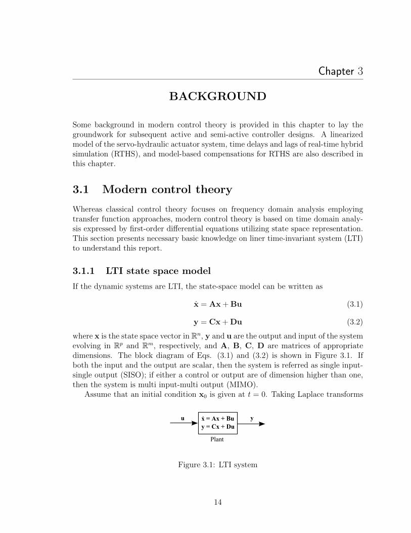
If the dynamic systems are LTI, the state-space model can be written as
x = Ax + Bu (3.1)
y = Cx + Du (3.2)
where x is the state space vector in Rn, y and u are the output and input of the systemevolving in Rp and Rm, respectively, and A, B, C, D are matrices of appropriatedimensions. The block diagram of Eqs. (3.1) and (3.2) is shown in Figure 3.1. Ifboth the input and the output are scalar, then the system is referred as single input-single output (SISO); if either a control or output are of dimension higher than one,then the system is multi input-multi output (MIMO).
Assume that an initial condition x0 is given at t = 0. Taking Laplace transforms
Plant
yu x = Ax + Bu
y = Cx + Du
Figure 3.1: LTI system
14

in Eqs. (3.1) and (3.2) gives the transformed equations:
sX− x0 = AX(s) + BU(s) (3.3)
Y(s) = CX(s) + DU(s) (3.4)
Solving for X(s) givesX(s) = Φ(s)x0 + Φ(s)BU(s) (3.5)
whereΦ(s) = [sI−A]−1. (3.6)
This is converted into the time domain by taking inverse Laplace transforms. Define
φ(t) = L−1{Φ(s)} = L−1{[sI−A]−1} (3.7)
where the inverse Laplace transform of Φ(s) is calculated term by term. Using con-volution, Eq. (3.5) can be inverted to give
x(t) = φ(t)x0 +
∫ t
0
φ(t− τ)Bu(τ)dτ (3.8)
As for the output, assuming for simplicity that x0 = 0 and substituting Eq. (3.5)into Eq. (3.4) gives
Y(s) = CΦ(s)BU(s) + DU(s) (3.9)
Therefore the transfer function is a p × m matrix-valued function of s which takesthe form
G(s) = CΦ(s)B + D (3.10)
Taking the inverse Laplace transform of the transfer function yields the impulse re-sponse
g(t) = L−1{G(s)} = Cφ(t)B + Dδ(t) (3.11)
where δ(t) is Dirac delta function defined as
δ(t) =
{+∞ t = 0
0 t 6= 0(3.12)
∫ ∞−∞
δ(t)dt = 1 (3.13)
Thus, the output is given for zero initial conditions by
y(t) = g ∗ u(t) =
∫ t
0
g(t− τ)u(τ)dτ =
∫ t
0
Cφ(t− τ)Bu(τ)dτ + Du(t) (3.14)
where ∗ represents convolution integral.
15

Plant
Controller
x
y
u
-K
x = Ax + Bu
y = Cx + Du
Figure 3.2: State feedback
3.1.2 State feedback
Assuming that all of the states are available, the simplest controller is given by thestate feedback control law
u = −Kx (3.15)
where K is a n×m matrix. Substituting this input u into Eq. (3.1) gives rise to theclosed-loop system written as
x = Ax−BKx = (A−BK)x (3.16)
The block diagram of this closed-loop system is shown in Figure 3.2.To determine whether or not x(t) → 0 as t → ∞ from any initial condition, the
eigenvalues of the closed-loop matrix (A − BK) must be considered. If and only if(A,B) is a controllable pair, the eigenvalues of (A−BK) can be placed arbitrarily,respecting complex conjugate constraints.
3.1.3 Observers
The state feedback approach can be generalized to the situation where only partialmeasurements of the state are available. In this case, the state, x, should be estimatedfrom the input-output measurements online.
To mimic the behavior of the system given by Eq. (3.1), the estimated systemgiven as
˙x = Ax + Bu (3.17)
should be considered, where x is the estimated state for the state x. Defining theerror between the real state and the estimated state as
e = x− x (3.18)
from Eqs. (3.1) and (3.17), the error equation is given by
e = x− ˙x
= Ax + Bu−Ax−Bu
= Ae
(3.19)
16
Thuse = eAte(0) (3.20)
However, if the open-loop system is unstable, the error will not converge to zero andmay diverge to infinity for some initial conditions.
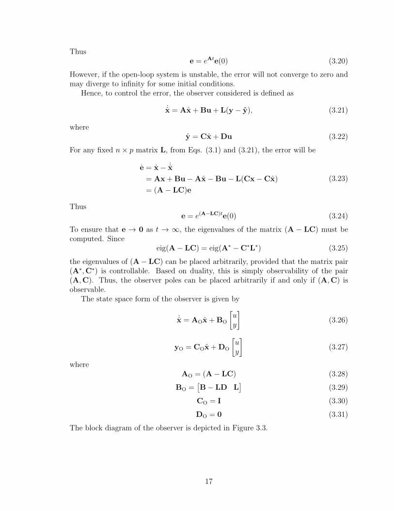
Hence, to control the error, the observer considered is defined as
˙x = Ax + Bu + L(y − y), (3.21)
wherey = Cx + Du (3.22)
For any fixed n× p matrix L, from Eqs. (3.1) and (3.21), the error will be
e = x− ˙x
= Ax + Bu−Ax−Bu− L(Cx−Cx)
= (A− LC)e
(3.23)
Thuse = e(A−LC)te(0) (3.24)
To ensure that e → 0 as t → ∞, the eigenvalues of the matrix (A − LC) must becomputed. Since
eig(A− LC) = eig(A∗ −C∗L∗) (3.25)
the eigenvalues of (A− LC) can be placed arbitrarily, provided that the matrix pair(A∗,C∗) is controllable. Based on duality, this is simply observability of the pair(A,C). Thus, the observer poles can be placed arbitrarily if and only if (A,C) isobservable.
The state space form of the observer is given by
˙x = AOx + BO
[uy
](3.26)
yO = COx + DO
[uy
](3.27)
whereAO = (A− LC) (3.28)
BO =[B− LD L
](3.29)
CO = I (3.30)
DO = 0 (3.31)
The block diagram of the observer is depicted in Figure 3.3.
17
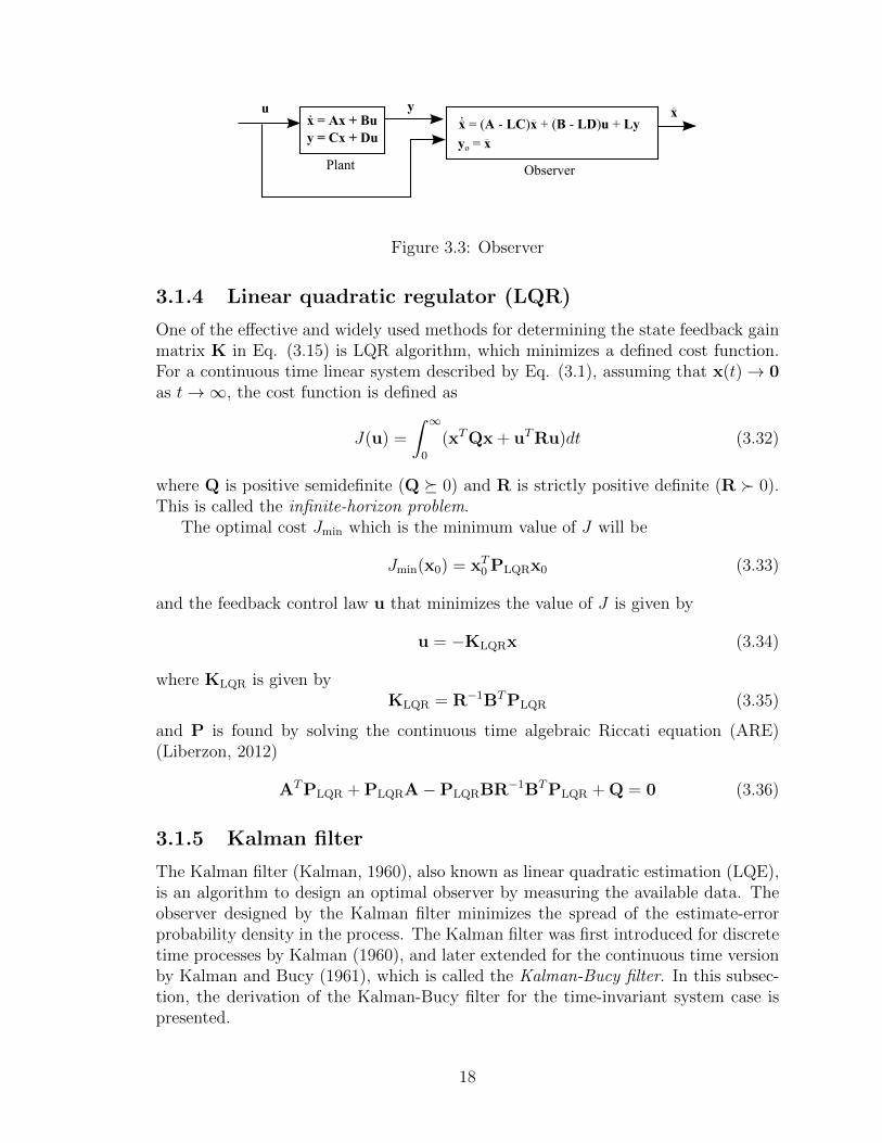
Plant
xyux = Ax + Bu
y = Cx + Dux = (A - LC)x + (B - LD)u + Ly
Observer
yo = x
Figure 3.3: Observer
3.1.4 Linear quadratic regulator (LQR)
One of the effective and widely used methods for determining the state feedback gainmatrix K in Eq. (3.15) is LQR algorithm, which minimizes a defined cost function.For a continuous time linear system described by Eq. (3.1), assuming that x(t)→ 0as t→∞, the cost function is defined as
J(u) =
∫ ∞0
(xTQx + uTRu)dt (3.32)
where Q is positive semidefinite (Q � 0) and R is strictly positive definite (R � 0).This is called the infinite-horizon problem.
The optimal cost Jmin which is the minimum value of J will be
Jmin(x0) = xT0 PLQRx0 (3.33)
and the feedback control law u that minimizes the value of J is given by
u = −KLQRx (3.34)
where KLQR is given byKLQR = R−1BTPLQR (3.35)
and P is found by solving the continuous time algebraic Riccati equation (ARE)(Liberzon, 2012)
ATPLQR + PLQRA−PLQRBR−1BTPLQR + Q = 0 (3.36)
3.1.5 Kalman filter
The Kalman filter (Kalman, 1960), also known as linear quadratic estimation (LQE),is an algorithm to design an optimal observer by measuring the available data. Theobserver designed by the Kalman filter minimizes the spread of the estimate-errorprobability density in the process. The Kalman filter was first introduced for discretetime processes by Kalman (1960), and later extended for the continuous time versionby Kalman and Bucy (1961), which is called the Kalman-Bucy filter. In this subsec-tion, the derivation of the Kalman-Bucy filter for the time-invariant system case ispresented.
18

Consider the linear time-invariant dynamic system expressed as
x = Ax + Bu + Ew (3.37)
y = Cx + Du + v (3.38)
Suppose that the expected values of the initial state and covariance are
E[x(0)] = x0 (3.39)
E{[x(0)− x0][x(0)− x0]T} = PKal,0 (3.40)
The disturbance input, w, is a white, zero-mean Gaussian random process such that
E[w(t)] = 0 (3.41)
E[w(t)wT (t)] = W(t)δ(t− τ) (3.42)
which is specified by its spectral density matrix W(t), and the measurement error,v, is a white, zero-mean Gaussian random process such that
E[v(t)] = 0 (3.43)
E[v(t)vT (t)] = V(t)δ(t− τ) (3.44)
with the measurement uncertainty expressed by its spectral density matrix V(t). Itis assumed that the disturbance input and measurement are uncorrelated.
In the Kalman-Busy filter, the optimal values of x(t) and the covariance ma-trix, PKal, can be computed as follows. First, the covariance estimate, PKal, can becalculated by solving the following ARE:
APKal + PKalAT + EWET −PKalC
TV−1CPKal = 0 (3.45)
The optimal filter gain equation is given using the obtained PKal by
LKal = PKalCTV−1 (3.46)
Then, the state estimate is found by integrating
˙x = Ax + Bu + LKal(y −Cx−Du) (3.47)
x(0) = x0 (3.48)
Note that the Kalman-Bucy filter problem is the mathematical dual of the LQRproblem.
3.1.6 Linear quadratic Gaussian (LQG)
To implement the LQR control, the full state information must be available. So, forthe case of the absence of the complete state data or the presence of uncertainties,
19

the LQG controller can be employed instead.The LQG controller is simply the combination of the Kalman filter with the LQR
controller. Consider the linear time-invariant dynamic system given by Eqs. (3.37)and (3.38). Given this system, the cost function of the LQG problem is defined as
J(u) = limτ→∞
E
[∫ τ
0
(xTQx + uTRu)dt
](3.49)
where Q is positive semidefinite (Q � 0), and R is positive definite (R � 0) as inthe case of the LQR. The objective is to find the control input u(t) which dependson the past measurements y(t′), 0 ≤ t′ < t.
The LQG controller that solves the LQG control problem is formulated by thefollowing equations:
˙x = Ax + Bu + LLQG(y −Cx−Du) (3.50)
u = −KLQGx (3.51)
Because the LQG controller can separate into the Kalman filter and the LQR prob-lems, the matrix gains LLQG and KLQG can be designed independently by solving theAREs given by Eqs. (3.36) and (3.45), respectively (Stengel, 1986). Hence, by Eqs.(3.35) and (3.46), each gain is given as
LLQG = LKal = R−1BTPLQR (3.52)
KLQG = KLQR = PKalCTV−1 (3.53)
Therefore the state-space form of the LQG controller can be expressed as
˙x = ALQGx + BLQGy (3.54)
yLQG = CLQGx + DLQGy (3.55)
whereALQG = A−BKLQR − LKalC + LKalDKLQR (3.56)
BLQG = LKal (3.57)
CLQG = −KLQR (3.58)
DLQG = 0 (3.59)
The block diagram of the LQG controller is depicted in Figure 3.4.
3.2 Servo-hydraulic system model
This section presents a model of a servo-hydraulic system.The servo-hydraulic systemis an assemblage of mechanical and electrical components used to excite a specimen,typically to a prescribed displacement as shown in Figure 3.5. Individual component
20

Plant
y
u = -KLQGx
x = Ax + Bu + Ew
y = Cx + Du + v
LQG controller
w
v
x = (A - BK - LC + LDK)x + LKaly
yLQG = -KLQGx
Figure 3.4: LQG controller
Actuator Specimen
Natural velocityfeedback
Servo-hydraulic sytem Gxu(s)
fu x+
- +
Servo-contorller
ec ic QLServo-valve
-
Figure 3.5: Block diagram model of the servo-hydraulic system
models can be assembled to create a dynamic model for the complete servo-hydraulicsystem. Components with nonlinear behavior will be represented by linear modelswith respect to an operating point such that the complete system model is also linear.The resulting linear model allows use of techniques such as Laplace transforms andfrequency domain methods to understand the system behavior.
3.2.1 Valve flow
The flow characteristics of the servo-valve are given by (Merritt, 1967)
QL = Cdwxv
√1
ρ
(Ps −
xv|xv|
pL
)(3.60)
where pL is the pressure drop across the load, QL is the controlled flow through theload, xv is the valve displacement from the neutral position, Ps is the system supplypressure, w is the opening ore area gradient of the valve orifices, Cd is the coefficient ofdischarge of the valve orifices, and ρ is the fluid density. The nonlinear flow equation
21
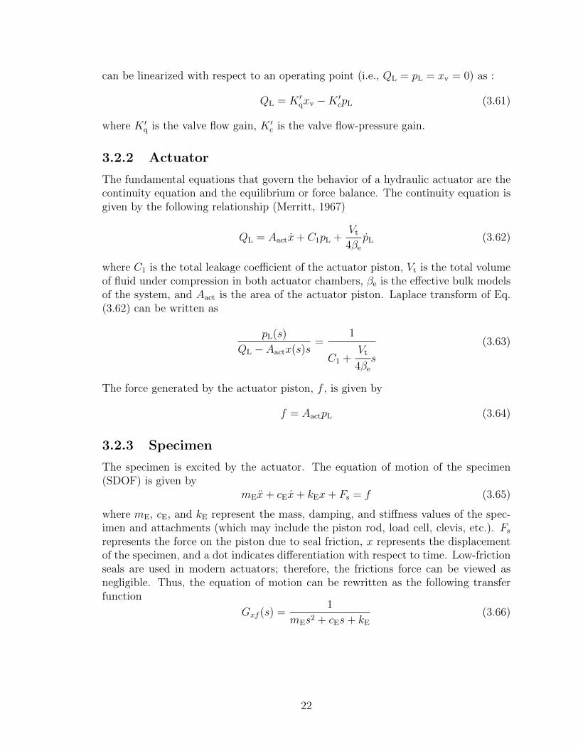
can be linearized with respect to an operating point (i.e., QL = pL = xv = 0) as :
QL = K ′qxv −K ′cpL (3.61)
where K ′q is the valve flow gain, K ′c is the valve flow-pressure gain.
3.2.2 Actuator
The fundamental equations that govern the behavior of a hydraulic actuator are thecontinuity equation and the equilibrium or force balance. The continuity equation isgiven by the following relationship (Merritt, 1967)
QL = Aactx+ C1pL +Vt4βe
pL (3.62)
where C1 is the total leakage coefficient of the actuator piston, Vt is the total volumeof fluid under compression in both actuator chambers, βe is the effective bulk modelsof the system, and Aact is the area of the actuator piston. Laplace transform of Eq.(3.62) can be written as
pL(s)
QL − Aactx(s)s=
1
C1 +Vt
4βes
(3.63)
The force generated by the actuator piston, f , is given by
f = AactpL (3.64)
3.2.3 Specimen
The specimen is excited by the actuator. The equation of motion of the specimen(SDOF) is given by
mEx+ cEx+ kEx+ Fs = f (3.65)
where mE, cE, and kE represent the mass, damping, and stiffness values of the spec-imen and attachments (which may include the piston rod, load cell, clevis, etc.). Fs
represents the force on the piston due to seal friction, x represents the displacementof the specimen, and a dot indicates differentiation with respect to time. Low-frictionseals are used in modern actuators; therefore, the frictions force can be viewed asnegligible. Thus, the equation of motion can be rewritten as the following transferfunction
Gxf (s) =1
mEs2 + cEs+ kE(3.66)
22
3.2.4 Servo-controller
Some type of control is needed to stabilize the system (Dyke et al., 1995), becausehydraulic actuators are inherently unstable. With displacement feedback, the errorsignal ec is defined by the difference between the command u and measured displace-ment x as
ec = u− x (3.67)
To eliminate the error, servo-controllers often use the Proportional-Integral-Derivative(PID) control given by
ic = Kpropec +Kint
∫ecdt+Kder
decdt
(3.68)
where ic is the electrical command signal to the servo-valve, and Kprop, Kint, andKdere are proportional, integral, and derivative gains, respectively. For real-time ap-plications, proportional gain alone is generally adequate, avoiding the lag introducedby integral control and sensitivity to noise of derivative control. Thus, the resultingcontrol law is given by
ic = Kpropec (3.69)
3.2.5 Servo-valve
The servo-valve provides an interface between the electrical and mechanical compo-nents of the system. The servo-valve receives an electrical signal from the servo-controller which moves the position of the valve spool, controlling the flow of oil intothe actuator.
For low frequencies, the servo-valve dynamics have been approximated by a con-stant (Merritt, 1967; Dyke et al., 1995; Zhao et al., 2006), as given by
xv = kvic (3.70)
where kv is the valve gain. In the Laplace domain, Eq. (3.70) can be written as
Gv =xv(s)
ic(s)= kv (3.71)
If a constant gain is inadequate over the frequency range of interest, a first-ordermodel including a time lag may be used. This transfer function is expressed as
Gv =kv
s+ τv(3.72)
where τv is the servo-valve time constant.
23
Actuator Specimen
Natural velocity feedback
Servo-hydraulic sytem Gxu(s)
fu x+
- -
Gv(s)
Aact
+
Servo-contorller
Servo-valvedynamics
Servo-valveflow
Kp QL = K'qxv - K'cpL
s
ec ic xv
Aact
QL
mEs2 + cEs + kE
11
C1 + Vts/(4βe)
pL
Figure 3.6: Block diagram model of the servo-hydraulic system
3.2.6 Combined model
The servo-hydraulic model can be obtained by combining the mathematical modelsof the controller, servo-valve, actuator, and specimen derived in 3.2.1 through 3.2.5.The block diagram of the combined model is shown in Figure 3.6.
The transfer function, Gxu(s), from the command displacement (input), u, to themeasured displacement (output), x, is obtained, in the case of constant servo-valvedynamics (Eq. (3.71)), as
Gxu(s) =Kp
KqAact
Kc
D3s3 +D2s2 +D1s+D0
(3.73)
whereKq = K ′qkv (3.74)
is the servo-valve gain,Kc = K ′cC1 (3.75)
is the total flow-pressure coefficient, and
D3 =Vt
4βeKc
mE (3.76)
D2 = mE +Vt
4βeKc
cE (3.77)
D1 = cE +Vt
4βeKc
kE +A2
act
Kc
(3.78)
D0 = kE +Kp
KqAact
Kc
(3.79)
24
The transfer function given by Eq. (3.73) has three poles and no zeros.In the case where a first-order model for the servo-valve dynamics (Eq. (3.72)) is
used, the transfer function can be expressed as
Gxu(s) =Kp
KqAact
Kc
D4s4 +D3s3 +D2s2 +D1s+D0
(3.80)
where
D4 =Vt
4βeKc
mEτv (3.81)
D3 =Vt
4βeKc
mE +mEτv +Vt
4βeKc
cEτv (3.82)
D2 = mE +Vt
4βeKc
cE +A2
act
Kc
τv + cEτv +Vt
4βeKc
kEτv (3.83)
D1 = cE +Vt
4βeKc
kE +A2
act
Kc
+ kEτv (3.84)
D0 = kE +KPKqAact
Kc
(3.85)
The transfer function given by Eq. (3.80) has four poles and no zeros.
3.3 Real-time hybrid simulation
RTHS is a variation of the hybrid simulation test method in which the imposeddisplacement and response analysis are conducted in real time. This is very power-ful strategy when the test specimen includes rate-dependent components. However,since RTHS is conducted in real time, the dynamics of the experimental system andspecimen affects the results.
3.3.1 Types of delays
In RTHS, there are inevitable experimental errors due to time delays and time lags.These are an intrinsic part of experimental testing and mitigation of their effects isan essential part of RTHS. Time delays and time lags are defined as follows.
Time delay
Time delays are generally caused by the communication of data, A/D and D/A dataconversion, and computation time. The transfer function for a pure time delay τis given by exp(−τs). So time delays have linear phases and constant magnitudes.These delays can be reduced by using faster hardware, smaller numerical integrationtime steps, and more efficient software.
25

Time lag
Time lags are a result of the physical dynamics and limitations of the servo-hydraulicactuators, i.e., control-structure-interaction (CSI). Therefore, time lags vary withboth the frequency of excitation and specimen conditions (Dyke et al., 1995). Thus,assuming a single time delay is not adequate over a wide frequency range to compen-sate the errors caused by time lags.
3.3.2 Experimental errors
The most significant experimental error in RTHS is poor phase tracking of the desireddisplacement. For a simple illustration, let the total time delays and time lags beapproximated as s single time delay Td. As shown in Figure 3.7(a), the measureddisplacement, x, is delayed from the desired displacement, d, by Td. Because of thisdelay, the force measured and fed back from the experiment does not correspond tothe desired displacement (it is measured before the actuator has reached its targetposition), however, the algorithm assumes that the measured force corresponds to thedesired displacement. If the specimen is linear-elastic, the resulting response, as seenby the algorithm, is a counter-clockwise hysteresis loop, instead of the straight linecorresponding to the linear behavior, as shown schematically in Figure 3.7(b). Thiscounterclockwise loop leads to additional energy into the structure. Horiuchi et al.(1996) demonstrated that for a SDOF system, the increase in the total system energycaused by the time delay/lag is equivalent to introducing negative damping into thesystem. This equivalent damping is given by
ceq = −kTd (3.86)
where k is the stiffness of the system. This artificial negative damping becomeslarge when either the stiffness of the system or the time delay/lag is large. Whenthis negative damping exceeds the structural damping, the system becomes unstable.Instability almost invariably occurs in practice due to the low levels of dampingassociated with structural frames and the large time delays/lags associated with largehydraulic actuators (Darby et al., 2001). Therefore, introducing compensation fortime delays/lags is essential in RTHS.
The effects of the time delays/lags have been traditionally treated together bydetermining a total delay that includes all of these effects. However, because the timelags vary with frequency, this approximation is valid only over the limited frequencyrange used for the approximation. If the conditions change significantly during thetest (e.g., natural frequency of the test structure due to changes in specimen stiff-ness), this method is not satisfactory because the system might become unstable(Blakeborough et al., 2001). Additionally, when the response of the test structure in-cludes significant contributions at different frequencies (e.g., MDOF), approximatingthe time lag with a single time delay may cause critical problems. While, the model-based compensators proposed in Carrion and Spencer (2007); Phillips and Spencer(2012) considers the effects of time lags for the wide frequency range. The details of
26

Desired d
Measured x
t
Displacement
Td
ActualResponse
MeasuredResponse
Displacement
Force
(a) (b)
Desired d
Measured x
Figure 3.7: Effects of time delay/lag; (a) Displacement history, (b) Force-deformationcurve
the model-based approach is described in the next section.
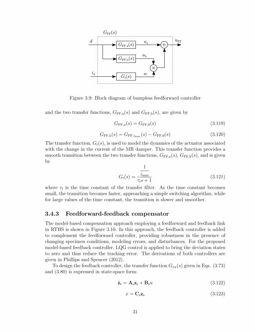
3.4 Model-based compensators for RTHS
To compensate time delays and lags caused by RTHS, a model-based actuator con-troller is designed. To achieve accurate displacements being imposed to specimens,RTHS needs an additional control scheme for compensating the inherent dynam-ics. As mentioned in Carrion and Spencer (2007); Phillips and Spencer (2012), amodel-based approach performs well for RTHS by extending the applicable frequencyrange, eliminating the lag in the loop, and enabling small damping used in the teststructure. In the model-based approach, the servo-hydraulic system is modeled by lin-earization over the actuator with the specimen as described in Section 3.2. Througha system identification technique, this model is refined to be capable of capturingthe command-to-displacement relationship. Based on this identified model, a model-based controller is designed to compensate the unexpected dynamics in RTHS. Ascheme of the compensated system is shown in Figure 3.8, in which the desired dis-placement, d, goes through the compensator, then the command displacement, u, isobtained such that the measured displacement of the specimen, x, becomes the sameas the desired displacement, d.
3.4.1 Feedforward compensator employing backwarddifference method
The feedforward controller is designed to cancel the modeled dynamic of the servo-hydraulic system. Placed in series with the servo-hydraulic system, the inverse of
27
Gxu(s)u x
Servo-hydraulicsystem
Compensatord
Figure 3.8: Compensation for actuator dynamics
the servo-hydraulic system model will serve as the feedforward controller, which isexpressed as
GFF(s) =1
Gxu
(s) (3.87)
Three-pole model
For the case that the three-pole model for the servo-hydraulic system, which is givenby Eq. (3.73), is used, from Eq. (3.87), the feedforward controller can be written as
GFF(s) = a0 + a1s+ a2s2 + a3s
3 (3.88)
where the coefficients a0 through a3 can be determined by expanding Eq. (3.87).Since the output of the feedforward controller is expressed as
UFF(s) = GFF(s)D(s) (3.89)
in the Laplace domain, the time domain expression is given by
uFF(t) = a0d(t) + a1d(1)(t) + a2d
(1)(t) + a3d(3)(t) (3.90)
where d(n) represents the nth derivative of d with respect to time. In discrete time,Eq. (3.90) can be written as
uFF,i = a0di + a1d(1)i + a2d
(2)i + a3d
(3)i (3.91)
Thus, the feedforward controller for the three-pole model servo-hydraulic systemrequires the calculation of displacement, velocity, acceleration, and jerk (derivativeof the acceleration) at time step i; however, most numerical integration schemes areonly explicit in displacement. In this report, backward difference method is used tocalculate the necessary higher-order derivatives. Note that this method is proposedsimply to estimate the higher-order derivatives at the required time step and can beselected independently from the numerical integration scheme.
The derivatives up to the fourth order calculated using the BDM are given by
d(1)i =
1
2∆t(3di − 4di−1 + di−2) (3.92)
28

d(2)i =
1
∆t2(2di − 5di−1 + 4di−2 − di−3) (3.93)
d(3)i =
1
2∆t3(5di − 18di−1 + 24di−2 − 14di−3 + 3di−4) (3.94)
where the derivatives are second order accurate. Substituting Eqs. (3.92) through(3.94) into Eq. (3.4.1) yields
uFF,i = b0di + b1di−1 + b2di−2 + b3di−3 + b4di−4 (3.95)
where
b0 = a0 +3a12∆t
+2a2∆t2
+5a3
2∆t3(3.96)
b1 =−2a1∆t
+−5a2∆t2
+−9a3∆t3
(3.97)
b2 =a1
2∆t+
4a2∆t2
+12a3∆t3
(3.98)
b3 =−a2∆t2
+−7a3∆t3
(3.99)
b4 =3a3
2∆t3(3.100)
Since the transfer function of the feedforward controller in discrete time is defined as
GFF(z) =UFF(z)
D(z), (3.101)
the transfer function of the feedforward compensator is expressed as
GFF(z) = b0 + b1z−1 + b2z
−2 + b3z−3 + b4z
−4 (3.102)
Four-pole model
In a similar way, the feedforward controller employing BDM for the four-pole modelservo-hydraulic system is derived. The feedforward controller in s-domain is given as
GFF(s) = a0 + a1s+ a2s2 + a3s
3 + a4s4 (3.103)
where the coefficients a0 through a4 can be determined by expanding Eq. (3.87). ByEq. (3.89), the output of the feedforward controller is given in continuous time by
uFF(t) = a0d(t) + a1d(1)(t) + a2d
(1)(t) + a3d(3)(t) + a4d
(4)(t) (3.104)
and, in discrete time, by
uFF,i = a0di + a1d(1)i + a2d
(2)i + a3d
(3)i + a4d
(4)i (3.105)
Therefore, when the four-pole model is used, jounce (derivative of the jerk) must
29
be calculated in addition to displacement, velocity, acceleration, and jerk at time stepi. The jounce obtained from BDM is given by
d(4)i =
1
∆t4(3di − 14di−1 + 26di−2 − 24di−3 + 11di−4 − 2di−5) (3.106)
Substituting Eqs. (3.92), (3.93), (3.94), and (3.106) into gives
uFF,i = b0di + b1di−1 + b2di−2 + b3di−3 + b4di−4 + b5di−5 (3.107)
where
b0 = a0 +3a12∆t
+2a2∆t2
+5a3
2∆t3+
3a4∆t4
(3.108)
b1 =−2a1∆t
+−5a2∆t2
+−9a3∆t3
+−14a4
∆t4(3.109)
b2 =a1
2∆t+
4a2∆t2
+12a3∆t3
+26a4∆t4
(3.110)
b3 =−a2∆t2
+−7a3∆t3
+−24a4
∆t4(3.111)
b4 =3a3
2∆t3+
11a4∆t4
(3.112)
b5 =−2a4∆t4
(3.113)
Hence, the feedforward controller employing BDM for the four-pole model is given as
GFF(z) = b0 + b1z−1 + b2z
−2 + b3z−3 + b4z
−4 + b5z−5 (3.114)
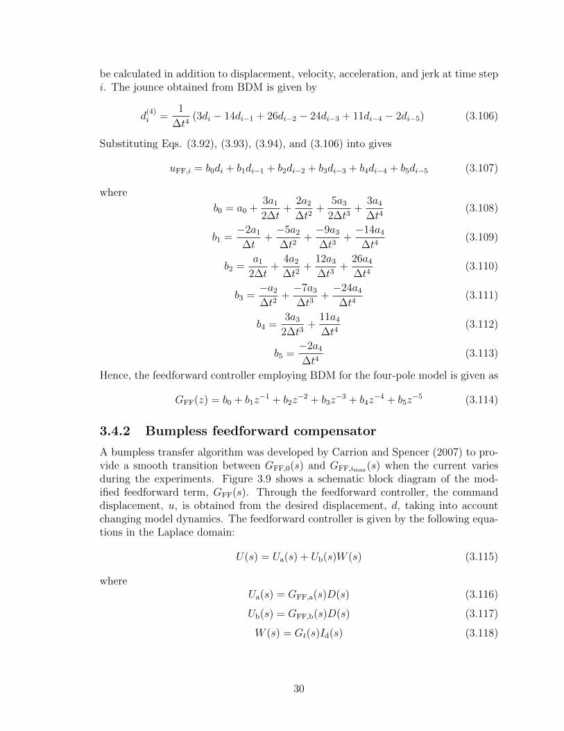
3.4.2 Bumpless feedforward compensator
A bumpless transfer algorithm was developed by Carrion and Spencer (2007) to pro-vide a smooth transition between GFF,0(s) and GFF,imax(s) when the current variesduring the experiments. Figure 3.9 shows a schematic block diagram of the mod-ified feedforward term, GFF(s). Through the feedforward controller, the commanddisplacement, u, is obtained from the desired displacement, d, taking into accountchanging model dynamics. The feedforward controller is given by the following equa-tions in the Laplace domain:
U(s) = Ua(s) + Ub(s)W (s) (3.115)
whereUa(s) = GFF,a(s)D(s) (3.116)
Ub(s) = GFF,b(s)D(s) (3.117)
W (s) = Gt(s)Id(s) (3.118)
30
GFF,a(s)ua
w
d
id
+
GFF,b(s)
Gt(s)
GFF(s)
×
ub
uFF
Figure 3.9: Block diagram of bumpless feedforward controller
and the two transfer functions, GFF,a(s) and GFF,b(s), are given by
GFF,a(s) = GFF,0(s) (3.119)
GFF,b(s) = GFF,imax(s)−GFF,0(s) (3.120)
The transfer function, Gt(s), is used to model the dynamics of the actuator associatedwith the change in the current of the MR damper. This transfer function provides asmooth transition between the two transfer functions, GFF,a(s), GFF,b(s), and is givenby
Gt(s) =
1
imax
τts+ 1(3.121)
where τt is the time constant of the transfer filter. As the time constant becomessmall, the transition becomes faster, approaching a simple switching algorithm, whilefor large values of the time constant, the transition is slower and smoother.
3.4.3 Feedforward-feedback compensator
The model-based compensation approach employing a feedforward and feedback linkin RTHS is shown in Figure 3.10. In this approach, the feedback controller is addedto complement the feedforward controller, providing robustness in the presence ofchanging specimen conditions, modeling errors, and disturbances. For the proposedmodel-based feedback controller, LQG control is applied to bring the deviation statesto zero and thus reduce the tracking error. The derivations of both controllers aregiven in Phillips and Spencer (2012).
To design the feedback controller, the transfer function Gxu(s) given in Eqs. (3.73)and (3.80) is expressed in state-space form:
zs = Aszs + Bsu (3.122)
x = Cszs (3.123)
31
Feedforwardcontoller
Feedbackcontroller
Servo-hydraulicsystem
LQG+
+
+-
uFF
d -e uFB u x
GFF(s)
Gxu(s)
Figure 3.10: Block diagram of feedforward and feedback links
where zs is the state vector. The tracking error between the desired displacement dand measured displacement x is given by
e = d− x (3.124)
The command, u, should be chosen such that the tracking error is minimized. Ifperfect tracking, i.e., x = d, is achieved by only the feedforward controller, uFF, theideal system is described as
z = Aszi + BsuFF (3.125)
d = Cszi (3.126)
where zi is an ideal state. Deviations of the state from the ideal system with respectto the original system is defined as
zd = zs − zi (3.127)
and assume that deviation of the control is provided by a feedback controller, i.e.,
uFB = u− uFF (3.128)
Then, considering disturbance to the system, wf , and the measurement noise, vf , thestate-space representation of the deviation system is
zd = Aszd + BsuFB + Eswf (3.129)
−e = Cszd + vf (3.130)
where Es is a matrix that describes how the disturbance enters the system.To improve the LQG controller’s performance and robustness in the frequency
range of interest, the disturbance, wf , is assumed to be Gaussian white-noise, w,passed through a second-order shaping filter, i.e.,
zf = Afzf + Efw (3.131)
wf = Cfzf (3.132)
32
where
Af =
[0 1−ω2
f −2ηfωf
](3.133)
Ef =
[01
](3.134)
Cf =[ω2f 2ξfηfωf
](3.135)
and zf is the state vector the shaping filter, zf is its time derivative, and the parametersξf , ωf , and ηf control the peak, bandwidth, and roll-off of the disturbance, respectively.The deviation system can be rewritten as an augmented system that includes thedynamics of the shaping filter. Defining the state
zFB =
[zTfzTd
], (3.136)
this augmented system is given by
zFB = AFBzFB + BFBuFB + EFBw (3.137)
−e = CFBzFB + vf (3.138)
where
AFB =
[Af 0
EsCf As
](3.139)
BFB =
[0Bs
](3.140)
EFB =
[Ef
0
](3.141)
CFB =[0 Cs
](3.142)
and the measurement noise vector, vf , is assumed to be comprised of independentGaussian white noises.
The control uFB can be obtained using LQR design assuming full state feedbackand output weighting as follows
JFB =
∫ ∞0
{QFB(−e)2 +RFB(uFB)2}dt (3.143)
uFB = −KFBzFB (3.144)
where KFB is the optimal state feedback gain matrix, JFB is the cost function mini-mized by LQR design, QFB is the weighting matrix on the system outputs, and RFB
is the weighting matrix on the system inputs.The augmented system states za can be estimated using a Kalman filter
˙zFB = AFBzFB + BFBuFB + LFB(−e−CFBzFB) (3.145)
33
where zFB represents the estimated states and LFB is the optimal observer gain matrix.The control law in Eq. (3.144) is then written in terms of the estimated states
and included in the estimator
˙zFB = (AFB − LFBCFB −BFBKFB)zFB + LFB(−e) (3.146)
uFB = −KFBzFB (3.147)
3.5 Summary
This chapter provided the background on modern control theory that is essential tothe development of the proposed research. In addition, the servo-hydraulic systemmodel, the effects of time delays/lags in RTHS, and the model-based compensatorsfor RTHS used in this report were described.
34
Chapter 4
MODELING AND EXPERIMENTAL SETUP
This chapter provides a model of the MR damper used throughout this report. Basedon the background presented in Chapter 3, a model of the servo-hydraulic system andcompensators for the system are designed for RTHS as well in this chapter.
4.1 MR damper modeling
The MR damper employed in this study is an RD-1005 MR fluid damper manu-factured by the Lord Corporation (Cary, NC, USA) and shown in Figure 4.1. Thedamper is 8.5 inch long in its extended position, and the main cylinder is 1.5 inchin diameter. The damper has a stroke of ±1.0 inch and can generate forces up toabout 500 lbf. The main cylinder of the damper accommodates the piston, the elec-tromagnet, an accumulator, and 50 ml of MR fluid. The magnetic field produced inthe device is generated by a small electromagnet in the piston head (Spencer et al.,1997). Input current commands are supplied to the damper using an RD-1002 Won-derbox from the Lord Corporation, which uses a modulated pulse-width amplifier togenerate a current in the MR damper circuit that is proportional to the applied volt-age. The maximum input current of the system imax is 2.0 A. By selecting the inputcurrent, the characteristics of the damper may be changed in real-time to vary theforces exerted by the damper. The power required by the MR damper is very small(less than 10 watts), and the system, damper and the current driver, has a responsetime of typically less than 10 msec (Spencer et al., 1997).
In this report, the MR damper is modeled by the phenomenological model (Spenceret al., 1997) as shown in Figure 4.2 in which the damper force is a function of thedamper displacement and velocity. The MR damper force fMR is given by
fMR = αz + c0(x− y) + k0(x− y) + k1x (4.1)
where x is the displacement of the MR damper, y is an internal displacement asillustrated in Figure 4.2, and z is an evolutionary variable (Wen, 1976) governed by
z = −γ|x− y|z|z|n−1 − β(x− y)|z|n + A(x− y). (4.2)
And k0, k1, c0, c1, α, β, γ, A, and n are parameters for the MR damper model.Since MR dampers are driven by currents, α, c0, c1, β and γ are current dependentvariables given by
α = αa + (αb − αa) tanh(αcic) (4.3)
c0 = c0a + (c0b − c0a) tanh(c0cic) (4.4)
35

(a)
(b)
Figure 4.1: Small-scale MR damper
c1 = c1a + (c1b − c1a) tanh(c1cic) (4.5)
β = βa + (βb − βa) tanh(βcic) (4.6)
γ = γa + (γb − γa) tanh(γcic) (4.7)
where ic is the input current to the MR damper model after a first order filter whichis designed to account for the time that the MR fluid takes to reach rheologicalequilibrium (Carrion and Spencer, 2007):
ic = −η(ic − id) (4.8)
where id is the desired current applied to the current driver and η is a parameterobtained experimentally.
To obtain the parameters of the MR damper, the damper is experimentally sub-jected to a 1 Hz sine wave with 1.02 cm (0.4 in) amplitude and constant currentof 0 A, 0.5 A, 1.0 A, 1.5 A, and 2.0 A. Then, the parameters are fit using nonlin-ear least squares parameter estimation to match the experimental response of thedamper. To decide the parameters, importance are placed especially on 0 A and 2.0A cases because 0 A (passive-off) and 2.0 A (passive-on) modes are used mainly inthis report. Table 4.1 provides the parameters obtained from MATLAB (MATLAB,2013) optimization toolbox. The comparisons between the experimental data andanalytical data by the created model are shown in Figures 4.3 through 4.7 for each
36

y
fMR
c1
k1
x
k0
c0
Figure 4.2: Mechanical model of the MR damper
Table 4.1: Parameters for the MR damper model
c0a 8.129 lbf·sec/in c0b 37.082 lbf·sec/in c0c 1.192 /Ak0 0.012 lbf/in k1 0.007 lbf/in x0 0 inc1a 406.314 lbf·sec/in c1b 786.564 lbf·sec/in c1c 0.315 /Aαa 18.361 lbf/in αb 100.617 lbf/in αc 0.551 /A
γa, βa 145.710 /in2 γb, βb 17.600 /in2 γc, βc 2.120 /AA 167.073 n 2 η 50 /sec
input current.
4.2 RTHS setup
RTHS consists of a computational model and physical specimen (the MR damper inthis report) in a loop, with an appropriate loading unit and testing equipment. Aschematic configuration for RTHS in this study is shown in Figure 4.8(a). Testinghardware in the RTHS includes a digital signal processor (DSP) running numericalintegration for the structure and generating the command signals, a small-scale MRdamper that is driven by a servo-hydraulic actuator, which is controlled by a servo-controller, and Analog-to-Digital (A/D) and Digital-to- Analog (D/A) converters forsignal processing. Sensors include a linear variable displacement transducer (LVDT)for displacement measurements and a load cell for measuring the MR damper force.
In Figure 4.8(a), u is the commanded displacement, fMR is the MR damper forcemeasured by the load cell, x is the displacement measured by the LVDT and i is thecontrol current sent to the hydraulic actuator. A detailed description of this RTHSimplementation can be found in Carrion and Spencer (2007). Figure 4.8(b) shows aphotograph of the experimental setup for RTHS. The experiments are conducted at
37

0 2 4 6 8 10 12 14 16
200
0
200
Time (sec)
Forc
e (N
)
Experiment Model
0.5 0 0.5
200
0
200
Displacement (in)
Forc
e (N
)
3 2 1 0 1 2 3
200
0
200
Velocity (in/sec)F
orc
e (N
)
Figure 4.3: MR damper force with 0 A to 0.4 in, 1.0 Hz sine wave
0 2 4 6 8 10 12 14 16
200
0
200
Time (sec)
Forc
e (N
)
Experiment Model
0.5 0 0.5
200
0
200
Displacement (in)
Forc
e (N
)
3 2 1 0 1 2 3
200
0
200
Velocity (in/sec)
Forc
e (N
)
Figure 4.4: MR damper force with 0.5 A to 0.4 in, 1.0 Hz sine wave
38
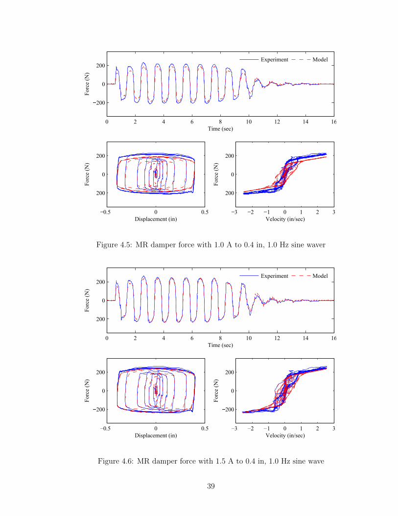
0 2 4 6 8 10 12 14 16
200
0
200
Time (sec)
Forc
e (N
)
Experiment Model
0.5 0 0.5
200
0
200
Displacement (in)
Forc
e (N
)
3 2 1 0 1 2 3
200
0
200
Velocity (in/sec)F
orc
e (N
)
Figure 4.5: MR damper force with 1.0 A to 0.4 in, 1.0 Hz sine waver
0 2 4 6 8 10 12 14 16
200
0
200
Time (sec)
Forc
e (N
)
Experiment Model
0.5 0 0.5
200
0
200
Displacement (in)
Forc
e (N
)
3 2 1 0 1 2 3
200
0
200
Velocity (in/sec)
Forc
e (N
)
Figure 4.6: MR damper force with 1.5 A to 0.4 in, 1.0 Hz sine wave
39
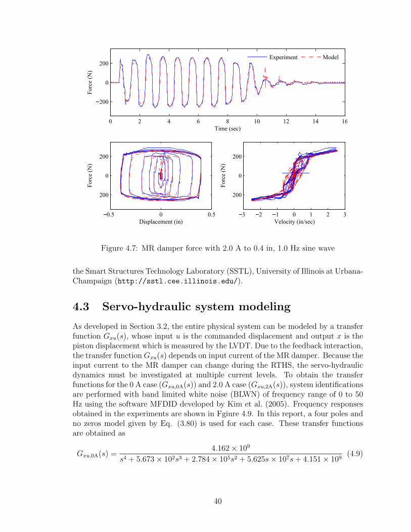
0 2 4 6 8 10 12 14 16
200
0
200
Time (sec)
Forc
e (N
)
Experiment Model
0.5 0 0.5
200
0
200
Displacement (in)
Forc
e (N
)
3 2 1 0 1 2 3
200
0
200
Velocity (in/sec)F
orc
e (N
)
Figure 4.7: MR damper force with 2.0 A to 0.4 in, 1.0 Hz sine wave
the Smart Structures Technology Laboratory (SSTL), University of Illinois at Urbana-Champaign (http://sstl.cee.illinois.edu/).
4.3 Servo-hydraulic system modeling
As developed in Section 3.2, the entire physical system can be modeled by a transferfunction Gxu(s), whose input u is the commanded displacement and output x is thepiston displacement which is measured by the LVDT. Due to the feedback interaction,the transfer function Gxu(s) depends on input current of the MR damper. Because theinput current to the MR damper can change during the RTHS, the servo-hydraulicdynamics must be investigated at multiple current levels. To obtain the transferfunctions for the 0 A case (Gxu,0A(s)) and 2.0 A case (Gxu,2A(s)), system identificationsare performed with band limited white noise (BLWN) of frequency range of 0 to 50Hz using the software MFDID developed by Kim et al. (2005). Frequency responsesobtained in the experiments are shown in Fgiure 4.9. In this report, a four poles andno zeros model given by Eq. (3.80) is used for each case. These transfer functionsare obtained as
Gxu,0A(s) =4.162× 10⁹
s4 + 5.673× 10²s3 + 2.784× 10⁵s2 + 5.625s× 107s+ 4.151× 10⁹(4.9)
40
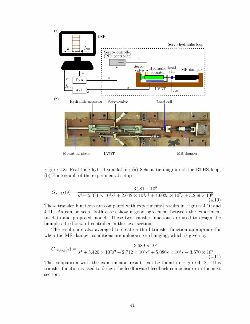
Servo-controller(PID controller)
Servo-hydraulic loop
Hydraulicactuator
DSP
LVDT
MR damperLoadcell
D/A
A/D
Servo-valve
u
xfMR
Mounting plate
Hydraulic actuator Servo-valve
LVDT MR damper
Load cell
(a)
(b)
x u
fMR
u
fMRu
Figure 4.8: Real-time hybrid simulation; (a) Schematic diagram of the RTHS loop,(b) Photograph of the experimental setup
Gxu,2A(s) =3.281× 10⁹
s4 + 5.371× 10²s3 + 2.642× 10⁵s2 + 4.602s× 107s+ 3.259× 10⁹
(4.10)These transfer functions are compared with experimental results in Figures 4.10 and4.11. As can be seen, both cases show a good agreement between the experimen-tal data and proposed model. These two transfer functions are used to design thebumpless feedforward controller in the next section.
The results are also averaged to create a third transfer function appropriate forwhen the MR damper conditions are unknown or changing, which is given by
Gxu,avg(s) =3.689× 10⁹
s4 + 5.420× 10²s3 + 2.712× 10⁵s2 + 5.080s× 107s+ 3.670× 10⁹
(4.11)The comparison with the experimental results can be found in Figure 4.12. Thistransfer function is used to design the feedforward-feedback compensator in the nextsection.
41

0 5 10 15 20 25 30 35 40 45 500.2
0.4
0.6
0.8
1
Frequency (Hz)
Mag
nit
ude
0 A
2 A
Avg
0 5 10 15 20 25 30 35 40 45 50200
150
100
50
0
Frequency (Hz)
Phas
e (d
eg)
0 5 10 15 20 25 30 35 40 45 5020
15
10
5
0
Frequency (Hz)
Tim
e la
g (
mse
c)
Figure 4.9: Frequency response from the experiments
4.4 Model-based compensator design for RTHS
In this section, two model-based compensators, i.e., bumpless feedforward and feedforward-feedback compensators, are designed based on the methods presented in Section 3.4.The transfer functions of the servo-hydraulic system obtained in Section 4.3 are ap-plied. To design the feedforward controllers for both compensators, the BDM, whoseaccuracy has been proven in Phillips and Spencer (2012), is used. The sampling time∆t used in this research is 5.0× 10⁻⁴ sec.
4.4.1 Bumpless feedforward compensator
The bumpless feedforward compensator is designed here. By using the BDM intro-duced in Subsection 3.4.1, GFF,0A and GFF,2A in discrete time are calculated fromEqs. (4.9) and (4.10), respectively, as
GFF,0A(z) =5∑
k=0
bk,0Az−k (4.12)
42

0 5 10 15 20 25 30 35 40 45 500.2
0.4
0.6
0.8
1
Frequency (Hz)
Mag
nit
ude
Experiment
Model
0 5 10 15 20 25 30 35 40 45 50200
150
100
50
0
Frequency (Hz)
Phas
e (d
eg)
0 5 10 15 20 25 30 35 40 45 5020
15
10
5
0
Frequency (Hz)
Tim
e la
g (
mse
c)
Figure 4.10: Comparison between the experimental data and obtained model for 0 Acase
where
b0,0A = 1.484× 10⁴, b1,0A = −6.503× 10⁴, b2,0A = 1.141× 10⁵,
b3,0A = −1.002× 10⁵, b4,0A = 4.393× 10⁴, b5,0A = −7.689× 10³.(4.13)
and
GFF,2A(z) =5∑
k=0
bk,2Az−k (4.14)
where
b0,2A = 3.756× 10³, b1,2A = −1.670× 10⁴, b2,2A = 2.969× 10⁴,
b3,2A = −2.637× 10⁴, b4,2A = 1.169× 10⁴, b5,2A = −2.065× 10³.(4.15)
Also, in this report, τt Eq. (3.121) is taken as 0.0048 sec (Carrion and Spencer,2007).
This bumpless feedforward compensator compensator is employed for the RTHSin Chapter 7.
43

0 5 10 15 20 25 30 35 40 45 500.2
0.4
0.6
0.8
1
Frequency (Hz)
Mag
nit
ude
Experiment
Model
0 5 10 15 20 25 30 35 40 45 50200
150
100
50
0
Frequency (Hz)
Phas
e (d
eg)
0 5 10 15 20 25 30 35 40 45 5020
15
10
5
0
Frequency (Hz)
Tim
e la
g (
mse
c)
Figure 4.11: Comparison between the experimental data and obtained model for 2.0A case
4.4.2 Feedforward-feedback compensator
In the feedforward-feedback compensator, the feedforward controller GFF is designedbased on the Gxu,avg(s) given by Eq. (4.11). Employing the BDM yields
GFF(z) =5∑
k=0
bkz−k (4.16)
where
b0 = 1.658× 10⁴, b1 = −7.282× 10⁴, b2 = 1.281× 10⁵,
b3 = −1.126× 10⁵, b4 = 4.947× 10⁴, b5 = −8.675× 10³.(4.17)
To design the feedback controller, the transfer function given by Eq. (4.11) istransformed into a state-space form expressed as Eqs. (3.122) and (3.123). Theparameters for the shaping filter given by Eqs. (3.131) and (3.132) are determined
44

0 5 10 15 20 25 30 35 40 45 500.2
0.4
0.6
0.8
1
Frequency (Hz)
Mag
nit
ude
Experiment
Model
0 5 10 15 20 25 30 35 40 45 50200
150
100
50
0
Frequency (Hz)
Phas
e (d
eg)
0 5 10 15 20 25 30 35 40 45 5020
15
10
5
0
Frequency (Hz)
Tim
e la
g (
mse
c)
Figure 4.12: Comparison between the experimental data and obtained model foraveraged case
by trial and error as
ξf = 0.7, ωf = 20× 2π, ηf = 0. (4.18)
Then, the parameters for the state-space form of the LQG feedback controller,AFB, BFB, CFB, and DFB, are calculated, in discrete time, as
AFB =
0.881 1 0 0 0 0−0.006 0.881 0.129 0.190 −0.166 −0.117
0 0 0.934 1 0 00 0 −0.004 0.934 −0.038 −0.0270 0 0 0 0.921 10 0 0 0 −0.036 0.921
, BFB =
0
0.2500
0.0570
0.051
,CFB =
[0.023 −0.484 0 0 0 0
], DFB = 0.
(4.19)
respectively. This feedback-feedforward compensator is employed for the RTHS in
45

Chapter 8.
4.5 Summary
This chapter provided the MR damper model used for numerical simulations in thisreport. The experimental setup for RTHS was presented and the servo-hydraulicsystem was identified. Also, the compensators based on the servo-hydraulic systemwere designed and their effectiveness was shown here. These compensators will beused for the RTHS verification studies later in this report.
46
Chapter 5
HYSTERESIS LOOPS PRODUCED BY ACTIVE
CONTROL FORCES
Active control methods have been applied to numerous civil structures in recent years.A significant amount of the research on active control methods has been based on full-state feedback using the linear quadratic regulator (LQR) control algorithm; becausemeasurement of the full state (i.e., the displacements and velocities of all DOFs)is difficult, such algorithms are impractical in full-scale implementations. Outputfeedback strategies based on measured acceleration at a limited number of points havebeen proposed and validated. However, a thorough understanding of the dissipativenature of the associated control forces and the way in which these forces protect thestructure have been elusive. Also, to unravel the relationship between the propertiesof active control forces and the responses will be helpful in designing and developingsemi-active controllers.
This chapter considers the hysteric behavior of the control forces produced by thewidely employed linear quadratic Gaussian (LQG)-based acceleration feedback con-trol strategies. Numerical simulation studies on one-story and three-story buildingswith active bracing are carried out.
5.1 Active control in acceleration feedback:
Problem formulation
Consider a structural system, excited by a one-dimensional earthquake loading, withan equation of motion given by
Msx + Csx + Ksx = Gsf −MsLsxg (5.1)
where f is the vector of control forces, xg is the ground acceleration, Ms, Cs, and Ks
are the mass, linear damping and stiffness matrices of the structure, respectively, andGs and Ls are the influence coefficient vectors of the control force and structural mass,respectively. x is the displacement vector, which is composed of the displacement ofeach floor relative to the ground. An over dot represents the time derivative.
A state-space representation of the equation of motion can be written as
z = Az + Bf + Exg (5.2)
ym = Cmz + Dmf + Fmxg + v (5.3)
ye = Cez + Def + Fexg (5.4)
47

where z is the state variable of the story displacements and velocities relative to thebase, that is,
z =[xT xT
]T(5.5)
ym is the vector corresponding to the measured outputs including absolute accelera-tions, v is an observation noise vector, ye is the vector corresponding to the regulatedoutputs that are used for evaluation of the system. The matrices A, B, and E aregiven as
A =
[0 I
−M−1s Ks −M−1
s Cs
](5.6)
B =
[0
M−1s Gs
](5.7)
E =
[0−Ls
](5.8)
And Cm, Ce, Dm, De, Fm, and Fe are appropriately chosen matrices correspondingto the associated output vectors. Acceleration feedback control strategies for thestructure described in Eqs. (5.2), (5.3), and (5.4) can be derived based on LQGmethods. For the control design, the absolute acceleration of the ground, xg, is takento be a stationary filtered white noise, and an infinite horizon performance index ischosen that weights the regulated output vector, ye; that is,
J = limτ→∞
1
τE
[∫ ∞0
{(Cez + Def)T Q (Cez + Def) + fTRf
}dt
](5.9)
where Q and R are called weighting matrices. Further, the observation noise isassumed to be an identically distributed, statistically independent Gaussian whitenoise process. The separation principle is invoked to allow the control and estimationproblems to be considered independently. The resulting controller is of the form(Stengel, 1994; Skelton, 1988)
f = −Kz (5.10)
where z is the estimated state vector obtained from the Kalman filter, and K is thefull state feedback gain matrix for the deterministic regulator problem given by
K = R−1(N + BTP) (5.11)
P is the solution of the algebraic Riccati equation given by
PA + AP−PBR−1BTP + Q = 0 (5.12)
andQ = CT
e QCe − NR−1NT (5.13)
R = R + DeTQDe (5.14)
A = A−BR−1NT (5.15)
48
The Kalman filter optimal estimator is given by
˙z = Az + Bf + L(ym −Cmz−Dmf − Fmxg) (5.16)
L = (SCm +WEFTm)R˜−1 (5.17)
where S is the solution of the algebraic Ricatti equation given by
SA˜ + A˜ TS− SG˜S + H˜ = 0 (5.18)
andA˜ = AT −CmR˜−1(WFmE) (5.19)
G˜ = CTmR˜−1Cm (5.20)
H˜ = WEET −W 2EFmR˜−1FmET (5.21)
R˜ = V +WFmFTm (5.22)
where W and V are magnitude of the constant two-sided spectral densities for thewhite noises used in the LQG control design. The controller given in Eq. (5.10)has been shown to be effective in protecting structural systems from seismic loading(Dyke et al., 1996b).
5.2 Hysteresis control force loops by numerical
simulations
To investigate the nature of the energy dissipation capabilities of acceleration feed-back control strategies clearly, first, a one-story building model shown in Figure 5.1(a)is considered. Subsequently, the three-story model shown in Figure 5.1(b) is inves-tigated to determine if the trends found in the one-story model are also seen inmulti-DOFs structures. The three-story building model was previously investigatedby Dyke et al. (1995, 1996a). Because the actuator is installed between the first floorand the ground, its displacement is equal to the displacement of the first floor ofthe structure relative to the ground. Here, xi, xi, xai and di represent relative dis-placement, relative velocity, absolute accelerations of ith floor, and inter-story driftbetween ith and (i − 1)th floor (i.e., xi − xi−1), respectively. f is the force in theactuator installed between the ground and the first floor.
The models are subjected to 1940 El Centro NS and 1995 JMA Kobe NS earth-quake records using numerical simulation. To satisfy scaling laws, the earthquakesmust be reproduced at five times the recorded rate. The time histories of the employedearthquake records are shown in Figure 5.2.
To explore how the weighting matrices affect the natural frequency, the dampingratio, and the hysteresis loops produced by the LQG controller, various values of theweighting matrices Q and R in Eq. (5.9) are employed. The earthquake input energy
49
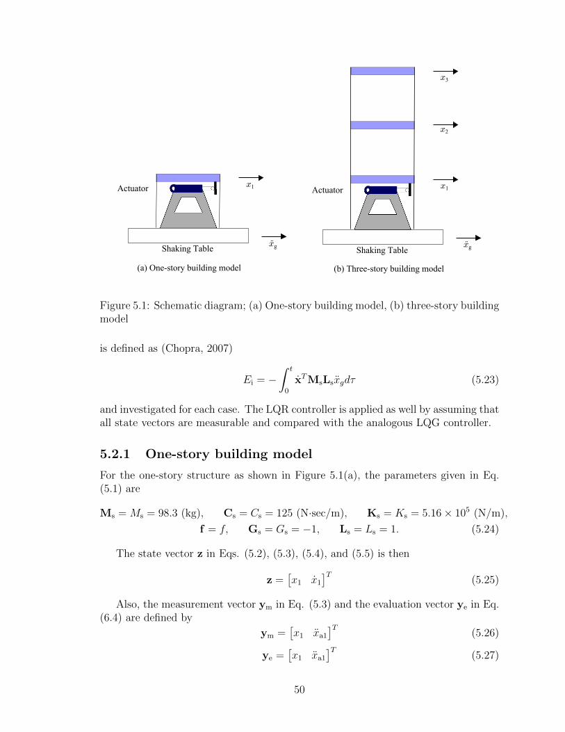
Shaking Table
Actuator
Shaking Table
Actuator
(a) One-story building model (b) Three-story building model
x1 x1
x2
x3
xg xg
Figure 5.1: Schematic diagram; (a) One-story building model, (b) three-story buildingmodel
is defined as (Chopra, 2007)
Ei = −∫ t
0
xTMsLsxgdτ (5.23)
and investigated for each case. The LQR controller is applied as well by assuming thatall state vectors are measurable and compared with the analogous LQG controller.
5.2.1 One-story building model
For the one-story structure as shown in Figure 5.1(a), the parameters given in Eq.(5.1) are
Ms = Ms = 98.3 (kg), Cs = Cs = 125 (N·sec/m), Ks = Ks = 5.16× 10⁵ (N/m),
f = f, Gs = Gs = −1, Ls = Ls = 1. (5.24)
The state vector z in Eqs. (5.2), (5.3), (5.4), and (5.5) is then
z =[x1 x1
]T(5.25)
Also, the measurement vector ym in Eq. (5.3) and the evaluation vector ye in Eq.(6.4) are defined by
ym =[x1 xa1
]T(5.26)
ye =[x1 xa1
]T(5.27)
50

0 1 2 3 4 5 6 7 8 9 10−4
−2
0
2
4
Time (sec)
Acc
eler
atio
n (
m/s
ec2)
(a)
0 1 2 3 4 5 6 7 8 9 10
−5
0
5
Time (sec)
Acc
eler
atio
n (
m/s
ec2)
(b)
Figure 5.2: Earthquake records; (a) 1940 El Centro NS, (b) 1995 JMA Kobe NS
respectively. Therefore, in this case, the matrices Cm, Ce, Dm, De, Em, and Ee canbe written as
Cm = Ce =
[1 0−Ks
Ms− Cs
Ms
], Dm = De =
[0Gs
Ms
], Fm = Fe = 02×1 (5.28)
Hence, the weighting matrices Q and R in Eq. (5.9) should be a 2 × 2 matrixand a scalar, R, respectively. Here, the weighting matrix Q is set as follows: all ofthe elements of the displacement weighting matrix Qd are zero, except for Qd11 = 1,and all of the elements of the acceleration weighting matrix Qa are zero, except forQa22 = 1. We assume that power spectral densities W and V are 5 × 10⁴ and I2×2,respectively. These values are determined by trial and error so that the LQG showsgood performance compared to the LQR controller. Calculations to determine K inEq. (5.11) and L in Eq. (5.17) are performed using the control toolbox in MATLAB(2013).
Figures 5.3 and 5.4 show how natural frequencies and damping ratios are affectedby changing the value of R in the case of both displacement and acceleration weight-ings, respectively. From the separation theorem, the poles (i.e., natural frequenciesand damping ratios) obtained by the LQG are the sum of the poles from the LQR andthe Kalman filter. From Figure 5.3, the actuator controlled by displacement weightedLQR and LQG results in the natural frequency of the building model increasing asthe control authority increases (i.e., R decreases), which means that the controlleradded positive stiffness to the structure. In contrast, Figure 5.4 shows that accelera-tion weighting leads to smaller natural frequency as the control authority is increased
51
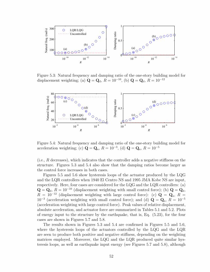
10�14
10�12
10�10
100
200
300
R
Nat
ura
l fr
eq. (r
ad/s
)(a)
(b)
LQR/LQG
Uncontrolled
10�14
10�12
10�10
0
0.5
1
R
Dam
pin
g r
atio
(a)
(b)
Figure 5.3: Natural frequency and damping ratio of the one-story building model fordisplacement weighting; (a) Q = Qd, R = 10−10, (b) Q = Qd, R = 10−12
10�6
10�4
10�2
20
40
60
80
R
Nat
ura
l fr
eq. (r
ad/s
)
(c)
(d)
LQR/LQG
Uncontrolled
10�6
10�4
10�2
0
0.5
1
R
Dam
pin
g r
atio
(c)
(d)
Figure 5.4: Natural frequency and damping ratio of the one-story building model foracceleration weighting; (c) Q = Qa, R = 10−3, (d) Q = Qa, R = 10−5
(i.e., R decreases), which indicates that the controller adds a negative stiffness on thestructure. Figures 5.3 and 5.4 also show that the damping ratios become larger asthe control force increases in both cases.
Figures 5.5 and 5.6 show hysteresis loops of the actuator produced by the LQGand the LQR controllers when 1940 El Centro NS and 1995 JMA Kobe NS are input,respectively. Here, four cases are considered for the LQG and the LQR controllers: (a)Q = Qd, R = 10−10 (displacement weighting with small control force); (b) Q = Qd,R = 10−12 (displacement weighting with large control force): (c) Q = Qa, R =10−3 (acceleration weighting with small control force); and (d) Q = Qa, R = 10−5
(acceleration weighting with large control force). Peak values of relative displacement,absolute acceleration, and actuator force are summarized in Tables 5.1 and 5.2. Plotsof energy input to the structure by the earthquake, that is, Eq. (5.23), for the fourcases are shown in Figures 5.7 and 5.8.
The results shown in Figures 5.3 and 5.4 are confirmed in Figures 5.5 and 5.6,where the hysteresis loops of the actuators controlled by the LQG and the LQRare seen to produce both positive and negative stiffness, depending on the weightingmatrices employed. Moreover, the LQG and the LQR produced quite similar hys-teresis loops, as well as earthquake input energy (see Figures 5.7 and 5.8), although
52
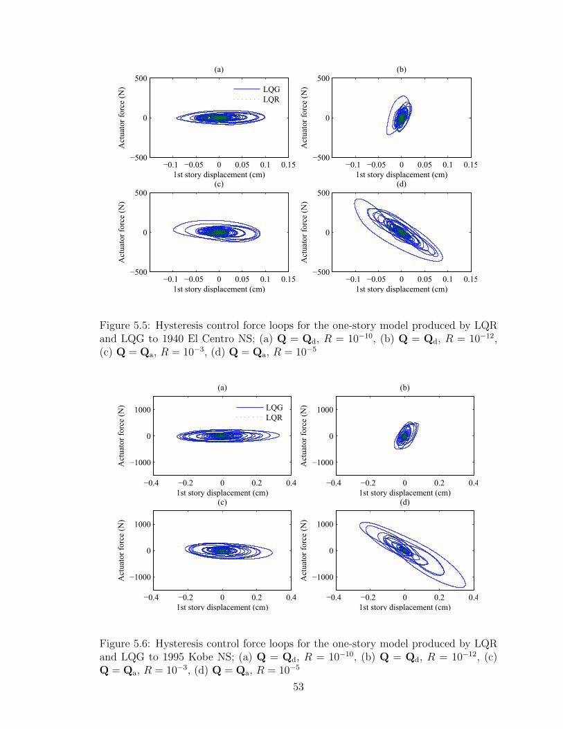
−0.1 −0.05 0 0.05 0.1 0.15−500
0
500
1st story displacement (cm)
Act
uat
or
forc
e (N
)
(a)
LQG
LQR
−0.1 −0.05 0 0.05 0.1 0.15−500
0
500
1st story displacement (cm)
Act
uat
or
forc
e (N
)
(b)
−0.1 −0.05 0 0.05 0.1 0.15−500
0
500
1st story displacement (cm)
Act
uat
or
forc
e (N
)
(c)
−0.1 −0.05 0 0.05 0.1 0.15−500
0
500
1st story displacement (cm)
Act
uat
or
forc
e (N
)
(d)
Figure 5.5: Hysteresis control force loops for the one-story model produced by LQRand LQG to 1940 El Centro NS; (a) Q = Qd, R = 10−10, (b) Q = Qd, R = 10−12,(c) Q = Qa, R = 10−3, (d) Q = Qa, R = 10−5
−0.4 −0.2 0 0.2 0.4
−1000
0
1000
1st story displacement (cm)
Act
uat
or
forc
e (N
)
(a)
LQG
LQR
−0.4 −0.2 0 0.2 0.4
−1000
0
1000
1st story displacement (cm)
Act
uat
or
forc
e (N
)
(b)
−0.4 −0.2 0 0.2 0.4
−1000
0
1000
1st story displacement (cm)
Act
uat
or
forc
e (N
)
(c)
−0.4 −0.2 0 0.2 0.4
−1000
0
1000
1st story displacement (cm)
Act
uat
or
forc
e (N
)
(d)
Figure 5.6: Hysteresis control force loops for the one-story model produced by LQRand LQG to 1995 Kobe NS; (a) Q = Qd, R = 10−10, (b) Q = Qd, R = 10−12, (c)Q = Qa, R = 10−3, (d) Q = Qa, R = 10−5
53
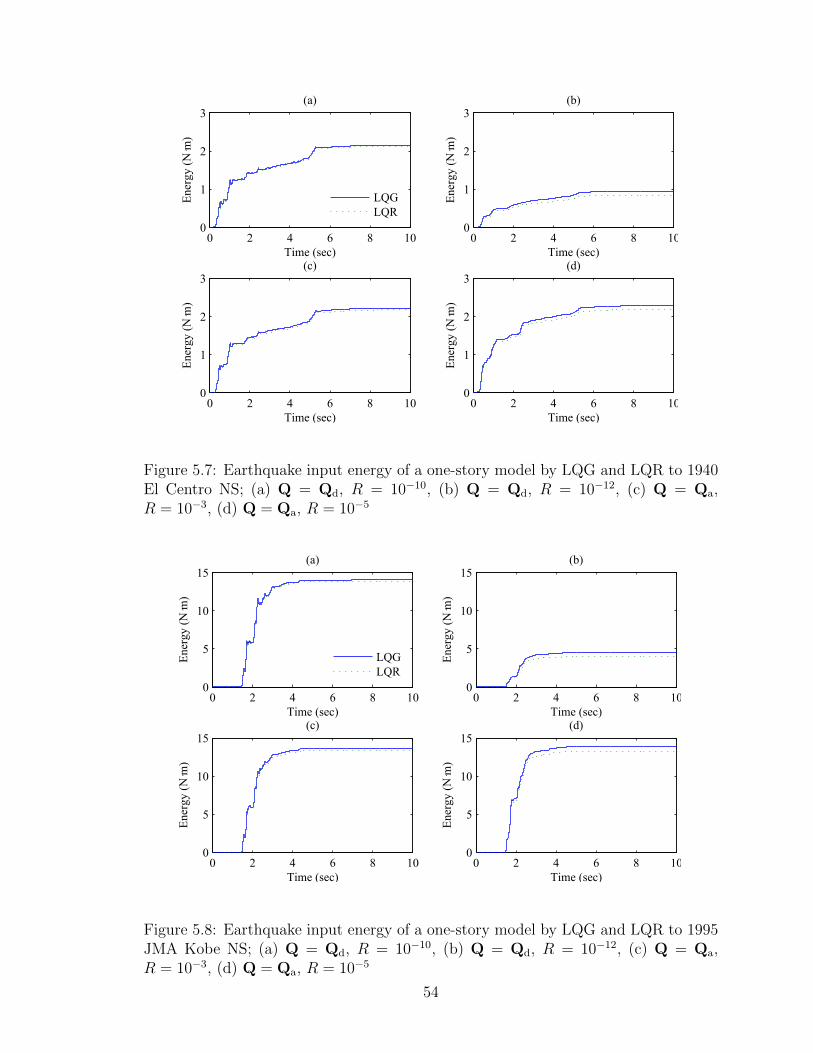
0 2 4 6 8 100
1
2
3
Time (sec)
Ener
gy (
N⋅m
)
(a)
LQG
LQR
0 2 4 6 8 100
1
2
3
Time (sec)
Ener
gy (
N⋅m
)
(b)
0 2 4 6 8 100
1
2
3
Time (sec)
Ener
gy (
N⋅m
)
(c)
0 2 4 6 8 100
1
2
3
Time (sec)
Ener
gy (
N⋅m
)
(d)
Figure 5.7: Earthquake input energy of a one-story model by LQG and LQR to 1940El Centro NS; (a) Q = Qd, R = 10−10, (b) Q = Qd, R = 10−12, (c) Q = Qa,R = 10−3, (d) Q = Qa, R = 10−5
0 2 4 6 8 100
5
10
15
Time (sec)
Ener
gy (
N⋅m
)
(a)
LQG
LQR
0 2 4 6 8 100
5
10
15
Time (sec)
Ener
gy (
N⋅m
)
(b)
0 2 4 6 8 100
5
10
15
Time (sec)
Ener
gy (
N⋅m
)
(c)
0 2 4 6 8 100
5
10
15
Time (sec)
Ener
gy (
N⋅m
)
(d)
Figure 5.8: Earthquake input energy of a one-story model by LQG and LQR to 1995JMA Kobe NS; (a) Q = Qd, R = 10−10, (b) Q = Qd, R = 10−12, (c) Q = Qa,R = 10−3, (d) Q = Qa, R = 10−5
54

Table 5.1: Peak values for the one-story model to 1940 El Centro NS; (a) Q = Qd,R = 10−10, (b) Q = Qd, R = 10−12, (c) Q = Qa, R = 10−3, (d) Q = Qa, R = 10−5
(a) (b) (c) (d)Parameter Uncontrolled LQG LQR LQG LQR LQG LQR LQG LQRx1 (cm) 0.173 0.099 0.098 0.032 0.029 0.099 0.097 0.102 0.097xa1 (m/s2) 9.098 5.389 5.310 3.798 3.728 4.995 4.957 3.404 3.333f (N) N/A 93.3 93.7 274.1 261.4 152.5 152.6 422.6 408.3
Table 5.2: Peak values for the one-story model to 1995 JMA Kobe NS; (a) Q = Qd,R = 10−10, (b) Q = Qd, R = 10−12, (c) Q = Qa, R = 10−3, (d) Q = Qa, R = 10−5
(a) (b) (c) (d)Parameter Uncontrolled LQG LQR LQG LQR LQG LQR LQG LQRx1 (cm) 0.641 0.332 0.327 0.078 0.070 0.291 0.285 0.352 0.336xa1 (m/s2) 33.674 17.819 17.687 8.885 8.758 14.758 14.599 8.977 8.796f (N) N/A 241.4 241.2 529.1 523.1 336.2 329.2 1404.8 1350.7
the LQR controller showed slightly better performance. Finally, Tables 5.1 and 5.2confirms that the displacement responses were reduced by the controller using dis-placement weighting, and the acceleration responses were reduced by the controllersusing acceleration weighting.
The next section investigates active control of a three-story model to see if thetrends found in the one-story controlled structure are also found in multi-DOF struc-tures.
5.2.2 Three-story building model
For the three-story structure as shown in Figure 5.1(b), the parameters for the equa-tion of motion given in Eq. (5.1) are
Ms =
98.3 0 00 98.3 00 0 98.3
(kg), Cs =
175 −50 0−50 100 −50
0 −50 50
(N·sec/m),
Ks = 105
12.0 −6.84 0−6.84 13.7 −6.84
0 −6.84 6.84
(N/m), f = f, Gs =
−100
, Ls =
111
(5.29)
55

The state vector z in Eqs. (5.2), (5.3), (5.4), and (5.5) is then
z =[x1 x2 x3 x1 x2 x3
]T(5.30)
Also, the measurement vector ym in Eq. (5.3) and the evaluation vector ye in Eq.(5.4) are defined by
ym =[x1 xa1 xa2 xa3
]T(5.31)
ye =[x1 d2 d3 xa1 xa2 xa3
]T(5.32)
Therefore, the matrices Cm, Ce, Dm, De, Em, and Ee become
Cm =
[1 0 0 01×3−M−1
s Ks −M−1s Cs
], Ce =
[∆ 03×3
−M−1s Ks −M−1
s Cs
],
∆ =
1 0 0−1 1 00 −1 1
, Dm =
[0
M−1s Gs
], De =
[03×1
M−1s Gs
],
Fm = 04×1, Fe = 06×1
(5.33)
Hence, the weighting matrices Q and R in Eq. (5.9) should be a 6×6 matrix anda scalar R, respectively. Here, two cases are considered. The first case weights thesecond and third inter-story drifts equally, whereas the weighting on the first floorrelative displacement is taken as a control design parameter α; that is
Qd = diag([α 1 1 0 0 0
])(5.34)
The second case places equal weighting on the acceleration of each floor of the struc-ture; that is,
Qa = diag([0 0 0 1 1 1
]) (5.35)
The power spectral densities of the disturbance W and the measurement noise vectorV are chosen to be 5×10⁴ and I4×4, respectively, so as to achieve comparable controlperformance with the LQR controller.
Figure 5.9 shows contours of the natural frequencies and damping ratios of first,second, and third modes for the displacement weighted LQR/LQG controllers as afunction of R and α. The natural frequencies of the uncontrolled model for threemodes are 34.2 rad/sec, 99.3 rad/sec, and 148.5 rad/sec, and noted in this figure bya heavier line weight. As can be seen here, the natural frequency of the first modeincreases as a increases, regardless of the value of R. This result indicates that thecontroller can produce both positive and negative stiffness contributions to the firstmode. Additionally, Fig. 5.9 shows that the natural frequencies of the second andthird modes are not substantially affected by α, and that the damping ratio increasesgenerally as the control force gets larger, as was the case of the one-story buildingmodel.
Figure 5.10 shows the natural frequencies and damping ratios of the first, sec-ond, and third modes as a function of R for acceleration weighting. For this case,
56

2530
35 40
45
50
Uncontrolled (34.2)
(a) (b)
(c) (d)
R
α
Natural freq. (rad/s) for 1st mode
10�14
10�12
10�10
10�2
10�1
100
101
0.60.50.4
0.3
0.2
0.20.1
(a) (b)
(c) (d)
R
α
Damping ratio for 1st mode
10�14
10�12
10�10
10�2
10�1
100
101
130
120110100
(a) (b)
(c) (d)
R
α
Natural freq. (rad/s) for 2nd mode
10�14
10�12
10�10
10�2
10�1
100
101
0.2
0.2
0.3
0.1
(a) (b)
(c) (d)
R
α
Damping ratio for 2nd mode
10�14
10�12
10�10
10�2
10�1
100
101
400
350
300250
200150
Uncontrolled (148.5)
(a) (b)
(c) (d)
R
α
Natural freq. (rad/s) for 3rd mode
10�14
10�12
10�10
10�2
10�1
100
101
0.60.5
0.40.3
0.20.1
(a) (b)
(c) (d)
R
α
Damping ratio for 3rd mode
10�14
10�12
10�10
10�2
10�1
100
101
Figure 5.9: Natural frequency and damping ratio of the three-story building modelfor displacement weighting; (a) Q = Qd(α = 1), R = 10−10, (b) Q = Qd(α = 1),R = 10−12, (c) Q = Qd(α = 0.01), R = 10−10.5, (d) Q = Qd(α = 0.01), R = 10−13.5
the natural frequencies of all modes decrease as the control force increases (i.e., Rdecreases); additionally, the damping ratio of the first mode increases as the controlforce is increased, which is again similar to the one-story model.
Six specific cases are considered for more investigation: (a) Q = Qd(α = 1),R = 10−10 (equal inter-story displacement weighting, with small control force); (b)Q = Qd(α = 1), R = 10−12 (equal inter-story displacement weighting, with largecontrol force); (c) Q = Qd(α = 0.01), R = 10−10.5 (inter-story displacement weightingmainly on the second and third stories, with small control force); (d) Q = Qd(α =0.01), R = 10−13.5 (inter-story displacement weighting mainly on the second andthird stories, with large control force); (e) Q = Qa, R = 10−3.5 (equal accelerationweighting, with small control force); and (f) Q = Qa, R = 10−5.5 (equal accelerationweighting, with large control force). These controllers are marked with an x in Figs.5.9 and 5.10. Figure 5.9 shows that controller (a) produces positive stiffness in all
57

10�6
10�4
10
20
30
40
R
Nat
ura
l fr
eq. (r
ad/s
)
1st mode
(e)(f)
LQR/LQG
Unontrolled
10�6
10�4
0
0.5
1
R
Dam
pin
g r
atio
1st mode
(e)
(f)
10�6
10�4
70
80
90
100
R
Nat
ura
l fr
eq. (r
ad/s
)
2nd mode
(e)
(f)
10�6
10�4
0
0.5
1
R
Dam
pin
g r
atio
2nd mode
(e)
(f)
10�6
10�4
140
145
150
R
Nat
ura
l fr
eq. (r
ad/s
)
3rd mode
(e)
(f)
10�6
10�4
0
0.5
1
R
Dam
pin
g r
atio
3rd mode
(e)(f)
Figure 5.10: Natural frequency and damping ratio of the three-story building modelfor acceleration weighting; (c) Q = Qa, R = 10−3.5, (d) Q = Qa, R = 10−5.5
modes, controller (b) produces positive stiffness in the first and second modes andnegative stiffness in third mode, and controllers (c), and (d) produce negative stiffnessin first mode and positive stiffness in second and third modes. Figure 5.10 shows thatcontrollers (e) and (f) produce negative stiffness in all three modes.
The hysteresis loops (i.e., control force versus displacement) for these six casesare shown in Figs. 5.11 and 5.12 for the structure subjected by the NS componentsof the 1940 El Centro and the 1995 JMA Kobe earthquakes. The dominance ofthe first mode in the response is seen in Figs. 5.11 and 5.12, that is, controllers(b) and (d) produce positive and negative stiffness, respectively. We can also seethat controller (f) has negative stiffness as in the case of one-story building model.Thus, the LQR/LQG can produce both positive and negative stiffness, depending onthe control weightings chosen. Moreover, the LQR and LQG hysteresis loops andearthquake input energies are nearly identical.
Peak values of relative displacement, inter-story drift, and absolute acceleration
58
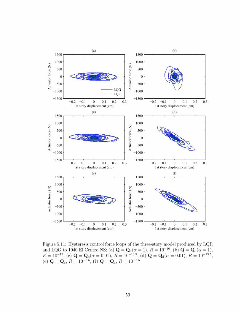
−0.2 −0.1 0 0.1 0.2 0.3−1500
−1000
−500
0
500
1000
1500
1st story displacement (cm)
Act
uat
or
forc
e (N
)(a)
LQG
LQR
−0.2 −0.1 0 0.1 0.2 0.3−1500
−1000
−500
0
500
1000
1500
1st story displacement (cm)
Act
uat
or
forc
e (N
)
(b)
−0.2 −0.1 0 0.1 0.2 0.3−1500
−1000
−500
0
500
1000
1500
1st story displacement (cm)
Act
uat
or
forc
e (N
)
(c)
−0.2 −0.1 0 0.1 0.2 0.3−1500
−1000
−500
0
500
1000
1500
1st story displacement (cm)
Act
uat
or
forc
e (N
)
(d)
−0.2 −0.1 0 0.1 0.2 0.3−1500
−1000
−500
0
500
1000
1500
1st story displacement (cm)
Act
uat
or
forc
e (N
)
(e)
−0.2 −0.1 0 0.1 0.2 0.3−1500
−1000
−500
0
500
1000
1500
1st story displacement (cm)
Act
uat
or
forc
e (N
)
(f)
Figure 5.11: Hysteresis control force loops of the three-story model produced by LQRand LQG to 1940 El Centro NS; (a) Q = Qd(α = 1), R = 10−10, (b) Q = Qd(α = 1),R = 10−12, (c) Q = Qd(α = 0.01), R = 10−10.5, (d) Q = Qd(α = 0.01), R = 10−13.5,(e) Q = Qa, R = 10−3.5, (f) Q = Qa, R = 10−5.5
59

−1 −0.5 0 0.5 1
−3000
−2000
−1000
0
1000
2000
3000
1st story displacement (cm)
Act
uat
or
forc
e (N
)(a)
LQG
LQR
−1 −0.5 0 0.5 1
−3000
−2000
−1000
0
1000
2000
3000
1st story displacement (cm)
Act
uat
or
forc
e (N
)
(b)
−1 −0.5 0 0.5 1
−3000
−2000
−1000
0
1000
2000
3000
1st story displacement (cm)
Act
uat
or
forc
e (N
)
(c)
−1 −0.5 0 0.5 1
−3000
−2000
−1000
0
1000
2000
3000
1st story displacement (cm)
Act
uat
or
forc
e (N
)
(d)
−1 −0.5 0 0.5 1
−3000
−2000
−1000
0
1000
2000
3000
1st story displacement (cm)
Act
uat
or
forc
e (N
)
(e)
−1 −0.5 0 0.5 1
−3000
−2000
−1000
0
1000
2000
3000
1st story displacement (cm)
Act
uat
or
forc
e (N
)
(f)
Figure 5.12: Hysteresis control force loops of the three-story model produced by LQRand LQG to 1995 JMA Kobe NS; (a) Q = Qd(α = 1), R = 10−10, (b) Q = Qd(α = 1),R = 10−12, (c) Q = Qd(α = 0.01), R = 10−10.5, (d) Q = Qd(α = 0.01), R = 10−13.5,(e) Q = Qa, R = 10−3.5, (f) Q = Qa, R = 10−5.5
60

for each floor, along with actuator force, are summarized in Tables 5.3 and 5.4. Whenthe control force is small (i.e., controllers (a), (c), and (e)), the controller has littleimpact on the responses. However, when the control force is large, the nature ofthe controllers is clearer; here, controllers (d) and (f) reduce absolute accelerationfor each floor more than controller (b). Again, the LQG controller has comparableperformance to its LQR counterpart.
61

Tab
le5.
3:P
eak
valu
esfo
rth
eth
ree-
stor
ym
odel
to19
40E
lC
entr
oN
S;
(a)
Q=
Qd(α
=1)
,R
=10−10,
(b)
Q=
Qd(α
=1)
,R
=10−12,
(c)
Q=
Qd(α
=0.
01),R
=10−10.5
,(d
)Q
=Q
d(α
=0.
01),R
=10−13.5
,(e
)Q
=Q
a,R
=10−3.5
,(f
)Q
=Q
a,
R=
10−5.5
(a)
(b)
(c)
(d)
(e)
(f)
Par
amet
erU
nco
ntr
olle
dL
QG
LQ
RL
QG
LQ
RL
QG
LQ
RL
QG
LQ
RL
QG
LQ
RL
QG
LQ
Rx1
(cm
)0.
541
0.23
00.
228
0.09
90.
096
0.24
00.
242
0.19
60.
192
0.21
20.
210
0.22
10.
216
x2
(cm
)0.
826
0.36
50.
362
0.16
20.
157
0.37
50.
377
0.22
00.
215
0.33
20.
327
0.25
80.
253
x3
(cm
)0.
964
0.45
80.
454
0.24
90.
242
0.46
10.
465
0.23
70.
231
0.40
10.
396
0.27
70.
272
d2
(cm
)0.
320
0.15
80.
157
0.13
10.
127
0.15
20.
154
0.04
10.
041
0.12
90.
127
0.05
60.
056
d3
(cm
)0.
202
0.09
90.
097
0.08
70.
085
0.09
30.
095
0.03
10.
031
0.07
70.
075
0.03
90.
038
xa1
(m/s
2)
8.66
44.
684
4.56
34.
069
3.92
84.
179
4.28
52.
690
2.65
33.
402
3.35
81.
601
1.58
3xa2
(m/s
2)
10.4
504.
905
4.81
94.
239
4.07
54.
615
4.69
11.
533
1.51
44.
107
4.03
41.
664
1.64
2xa3
(m/s
2)
14.0
616.
879
6.78
26.
084
5.93
86.
484
6.57
82.
167
2.13
65.
351
5.24
02.
686
2.64
7f
(N)
276.
627
5.5
944.
094
6.9
277.
227
8.7
887.
987
2.4
318.
231
2.7
874.
485
9.3
Tab
le5.
4:P
eak
valu
esfo
rth
eth
ree-
stor
ym
odel
to19
95JM
AK
obe
NS;
(a)
Q=
Qd(α
=1)
,R
=10−10,
(b)
Q=
Qd(α
=1)
,R
=10−12,
(c)
Q=
Qd(α
=0.
01),R
=10−10.5
,(d
)Q
=Q
d(α
=0.
01),R
=10−13.5
,(e
)Q
=Q
a,R
=10−3.5
,(f
)Q
=Q
a,
R=
10−5.5
(a)
(b)
(c)
(d)
(e)
(f)
Par
amet
erU
nco
ntr
olle
dL
QG
LQ
RL
QG
LQ
RL
QG
LQ
RL
QG
LQ
RL
QG
LQ
RL
QG
LQ
Rx1
(cm
)1.
490
0.83
10.
827
0.32
60.
318
0.85
70.
827
0.45
60.
408
0.80
60.
797
0.53
70.
528
x2
(cm
)2.
372
1.35
11.
343
0.58
30.
564
1.36
71.
321
0.52
70.
517
1.28
11.
265
0.67
40.
662
x3
(cm
)2.
883
1.66
51.
653
0.78
60.
762
1.67
11.
617
0.58
40.
608
1.56
01.
539
0.76
70.
752
d2
(cm
)0.
895
0.53
70.
532
0.37
20.
364
0.52
40.
510
0.14
10.
230
0.49
00.
483
0.20
50.
202
d3
(cm
)0.
529
0.31
50.
312
0.20
60.
203
0.30
60.
298
0.08
90.
140
0.28
20.
278
0.12
20.
120
xa1
(m/s
2)
23.3
4911
.521
11.2
838.
812
8.52
110
.558
10.1
894.
619
5.70
28.
753
8.48
53.
865
3.81
5xa2
(m/s
2)
27.9
8315
.960
15.7
8211
.951
11.6
7315
.554
15.1
414.
122
7.08
914
.617
14.3
865.
790
5.71
6xa3
(m/s
2)
36.8
3021
.911
21.7
1014
.345
14.0
9121
.294
20.7
196.
185
9.75
019
.616
19.3
278.
480
8.36
5f
(N)
932.
092
4.8
2367
.223
86.8
926.
997
5.4
2322
.723
08.0
1204
.211
89.8
2154
.321
19.9
62

The plots of earthquake energy input to the structure as given by Eq. (5.23) areshown in Figures 5.13 and 5.14 for cases (a)–(h). For both earthquakes, controller (b)shows the best performance. However, considering the peak actuator forces given inTables 5.3 and 5.4, controllers producing negative stiffness (i.e., controllers (d) and(h)) are more effective at limiting the input earthquake energy than the controllerscontrollers (b) and (f).
5.3 Summary
This chapter investigated the nature of the hysteric behavior of the control forcesproduced by the widely employed LQG-based acceleration feedback control strategy.Numerical simulation studies carried out on one-story and three-story buildings withactive bracing show that the LQG-based algorithms are quite versatile and can pro-duce controllers with a variety of behaviors depending upon the control objectiveschosen. Additionally, the numerical results demonstrated that the presented LQG-based acceleration feedback control had performance comparable to the LQR in thepresented SDOF and 3DOF building models.
63

0 2 4 6 8 100
2
4
6
8
10
12
Time (sec)
Ener
gy (
N*m
)(a)
LQG
LQR
0 2 4 6 8 100
2
4
6
8
10
12
Time (sec)
Ener
gy (
N*m
)
(b)
0 2 4 6 8 100
2
4
6
8
10
12
Time (sec)
Ener
gy (
N*m
)
(c)
0 2 4 6 8 100
2
4
6
8
10
12
Time (sec)
Ener
gy (
N*m
)
(d)
0 2 4 6 8 100
2
4
6
8
10
12
Time (sec)
Ener
gy (
N*m
)
(e)
0 2 4 6 8 100
2
4
6
8
10
12
Time (sec)
Ener
gy (
N*m
)
(f)
Figure 5.13: Earthquake input energy of the three-story model by LQG and LQR to1940 El Centro NS; (a) Q = Qd(α = 1), R = 10−10, (b) Q = Qd(α = 1), R = 10−12,(c) Q = Qd(α = 0.01), R = 10−10.5, (d) Q = Qd(α = 0.01), R = 10−13.5, (e) Q = Qa,R = 10−3.5, (f) Q = Qa, R = 10−5.5
64
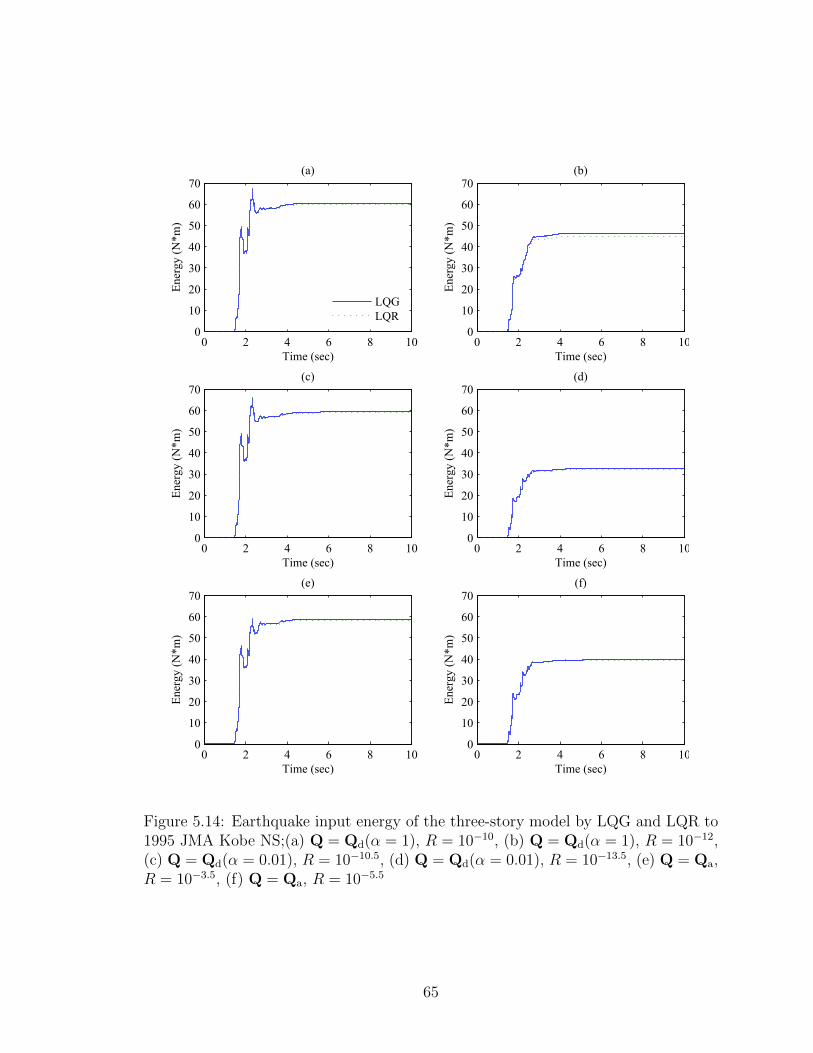
0 2 4 6 8 100
10
20
30
40
50
60
70
Time (sec)
Ener
gy (
N*m
)(a)
LQG
LQR
0 2 4 6 8 100
10
20
30
40
50
60
70
Time (sec)
Ener
gy (
N*m
)
(b)
0 2 4 6 8 100
10
20
30
40
50
60
70
Time (sec)
Ener
gy (
N*m
)
(c)
0 2 4 6 8 100
10
20
30
40
50
60
70
Time (sec)
Ener
gy (
N*m
)
(d)
0 2 4 6 8 100
10
20
30
40
50
60
70
Time (sec)
Ener
gy (
N*m
)
(e)
0 2 4 6 8 100
10
20
30
40
50
60
70
Time (sec)
Ener
gy (
N*m
)
(f)
Figure 5.14: Earthquake input energy of the three-story model by LQG and LQR to1995 JMA Kobe NS;(a) Q = Qd(α = 1), R = 10−10, (b) Q = Qd(α = 1), R = 10−12,(c) Q = Qd(α = 0.01), R = 10−10.5, (d) Q = Qd(α = 0.01), R = 10−13.5, (e) Q = Qa,R = 10−3.5, (f) Q = Qa, R = 10−5.5
65
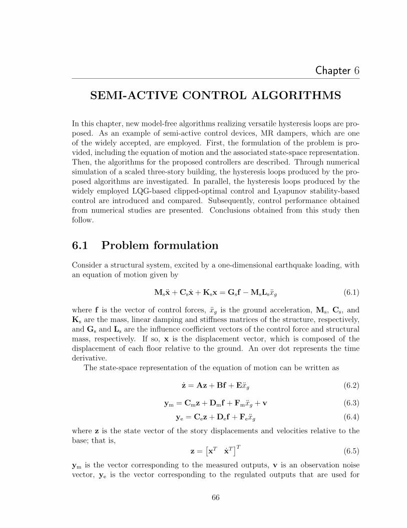
Chapter 6
SEMI-ACTIVE CONTROL ALGORITHMS
In this chapter, new model-free algorithms realizing versatile hysteresis loops are pro-posed. As an example of semi-active control devices, MR dampers, which are oneof the widely accepted, are employed. First, the formulation of the problem is pro-vided, including the equation of motion and the associated state-space representation.Then, the algorithms for the proposed controllers are described. Through numericalsimulation of a scaled three-story building, the hysteresis loops produced by the pro-posed algorithms are investigated. In parallel, the hysteresis loops produced by thewidely employed LQG-based clipped-optimal control and Lyapunov stability-basedcontrol are introduced and compared. Subsequently, control performance obtainedfrom numerical studies are presented. Conclusions obtained from this study thenfollow.
6.1 Problem formulation
Consider a structural system, excited by a one-dimensional earthquake loading, withan equation of motion given by
Msx + Csx + Ksx = Gsf −MsLsxg (6.1)
where f is the vector of control forces, xg is the ground acceleration, Ms, Cs, andKs are the mass, linear damping and stiffness matrices of the structure, respectively,and Gs and Ls are the influence coefficient vectors of the control force and structuralmass, respectively. If so, x is the displacement vector, which is composed of thedisplacement of each floor relative to the ground. An over dot represents the timederivative.
The state-space representation of the equation of motion can be written as
z = Az + Bf + Exg (6.2)
ym = Cmz + Dmf + Fmxg + v (6.3)
ye = Cez + Def + Fexg (6.4)
where z is the state vector of the story displacements and velocities relative to thebase; that is,
z =[xT xT
]T(6.5)
ym is the vector corresponding to the measured outputs, v is an observation noisevector, ye is the vector corresponding to the regulated outputs that are used for
66

evaluation of the system. The matrices A, B, and E are given as
A =
[0 I
−M−1s Ks −M−1
s Cs
], B =
[0
−M−1s Gs
], E =
[0−L−1s
](6.6)
and Cm, Ce, Dm, De, Fm, and Fe are appropriately chosen matrices correspondingto the associated output vectors.
The vector of control force is defined as
f =[fMR,1 fMR,2 · · · fMR,n
]T(6.7)
where fMR,j, j = 1, 2, · · ·n is the jth measured MR damper output force.
6.2 LQG-based clipped-optimal control
The LQG based clipped-optimal control method for MR dampers (Dyke et al., 1996c,d;Spencer et al., 1997) is explained briefly. By reconsidering Eq. (6.2), the cost functionof the LQG control can be written as
J = limt→∞
1
tE
[∫ t
0
(yTe Qye + fTc Rfc
)dt
](6.8)
where Q and R are the weighting parameters; fc is a control force vector defined as
fc =[fc,1 fc,2 · · · fc,n
]T(6.9)
where fc,j, j = 1, 2, · · ·n is the jth calculated control force. E[·] means the expectedvalue of the quantity in brackets and t represents the time. By minimizing Eq. (6.8),the control force is a function of the structural states. In the LQG control, the Kalmanfilter estimates (Dyke et al., 1996c) the state based on the measured responses suchthat
˙z = Az + Bfc + L (ym −Cmz−Dmfc − Fmxg) (6.10)
fc = −Kcz (6.11)
where L is the Kalman gain; Kc is the optimal control gain found by minimizing Eq.(6.8); and z is the estimated state by the Kalman filter. The clipped-optimal controlalgorithms are used to convert the optimal control force of Eq. (6.11) to a desiredcommand current for the MR damper. The desired command current is given by
id,j = imaxH {(fc,j − fMR,j) fMR,j} (6.12)
where H{·} is the Heaviside function, id,j is the desired input current to the jth MRdamper; imax is the maximum input current, fc,j is the jth optimal control forcegenerated by Eq. (6.11) and fMR,j is the actual force generated by the jth MRdamper. The clipped-optimal controller logic is illustrated in Figure 6.1.
67
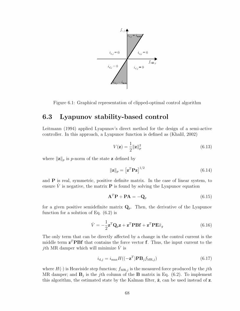
fMR,j
fc,j
Figure 6.1: Graphical representation of clipped-optimal control algorithm
6.3 Lyapunov stability-based control
Leitmann (1994) applied Lyapunov’s direct method for the design of a semi-activecontroller. In this approach, a Lyapunov function is defined as (Khalil, 2002)
V (z) =1
2‖z‖2p (6.13)
where ‖z‖p is p-norm of the state z defined by
‖z‖p =[zTPz
]1/2(6.14)
and P is real, symmetric, positive definite matrix. In the case of linear system, toensure V is negative, the matrix P is found by solving the Lyapunov equation
ATP + PA = −Qp (6.15)
for a given positive semidefinite matrix Qp. Then, the derivative of the Lyapunovfunction for a solution of Eq. (6.2) is
V = −1
2zTQpz + zTPBf + zTPExg (6.16)
The only term that can be directly affected by a change in the control current is themiddle term zTPBf that contains the force vector f . Thus, the input current to thejth MR damper which will minimize V is
id,j = imaxH((−zT )PBjfMR,j) (6.17)
where H(·) is Heaviside step function; fMR,j is the measured force produced by the jthMR damper; and Bj is the jth column of the B matrix in Eq. (6.2). To implementthis algorithm, the estimated state by the Kalman filter, z, can be used instead of z.
68
6.4 Model-free algorithms for semi-active control
In this section, new simple algorithms for use with MR dampers which do not requirethe structure model are introduced. Two model-free algorithms which can producepositive and pseudo-negative stiffness hysteresis loops are proposed herein. Let dj,dj, and da,j be the displacement, velocity, and absolute acceleration of the pistonof the jth MR damper. Figure 6.2 (a) and (b) depict the schematic illustrations ofdisplacement-force hysteresis loops for the cases of id,j = imax and id,j = 0, respec-tively.
6.4.1 Proposed simple algorithm 1
The first proposed algorithm controls the desired input current based on the sign ofthe product of the displacement and velocity of the MR damper. As shown in Figure6.2(c), to produce pseudo-negative stiffness, the desired input current is maximumwhen the direction of the displacement of the MR damper is different from that ofthe velocity and 0 when the displacement and velocity of the MR damper have thesame direction. Thus, the input current determined by
id,j = imaxH(−dj dj) (6.18)
can yield pseudo-negative stiffness by the MR damper.Positive stiffness can be realized by changing the sign in Eq. (6.18); i.e.,
id,j = imaxH(dj dj) (6.19)
In Eq. (6.19), imax input is applied when the directions of displacement and velocityare the same, otherwise it is 0. This is shown in Figure 6.2(d) schematically. Toimplement this algorithm, only sensors to measure the displacement and velocity ofthe devices are needed. In this report, the algorithms given by Eqs. (6.18) and (6.19)are named simple controller 1N and simple controller 1P, respectively.
6.4.2 Proposed simple algorithm 2
Another algorithm is obtained by measuring the displacement and the output forceof the MR damper. Pseudo-negative stiffness can be obtained when the desired inputcurrent is controlled as
id,j = imaxH(djfMR,j) (6.20)
as shown in Figure 6.2(c). In Eq. (6.20), the input current is the maximum when thedisplacement and output MR damper force have the same direction; otherwise it is0.
As shown in Figure 6.2(d), positive stiffness can be produced by controlling theinput current by
id,j = imaxH(−djfMR,j) (6.21)
69

(a) (b)
(c)
fMR,j
dj
id,j = imax
fMR,j
dj
id,j = 0
fMR,j
dj
id,j = imax
id,j = 0
id,j = imax
id,j = 0
(d)
fMR,j
dj
id,j = imax
id,j = 0
id,j = imax
id,j = 0
Figure 6.2: Schematic illustration of MR damper force; (a) id,j = imax, (b) id,j = 0,(c) Pseudo-negative stiffness, (d) Positive stiffness
In Eq. (6.20), the input current is maximum when the direction of the displacementand output MR damper force are different; otherwise it is 0.
6.5 Numerical simulation of the three-story
building model
To investigate the nature of the energy dissipation capabilities of the semi-activecontrollers described in the previous section through numerical studies, a buildingand MR damper model are presented in this section. Also, the two LQG-basedclipped-optimal controllers, i.e., acceleration and displacement weighting, and theLyapunov stability-based controller are designed.
6.5.1 Building model
The building model used in this study is a scaled three-story building model as shownin Figure 6.3 schematically. As can be seen, one MR damper is installed betweenthe ground and the first floor. This model was previously investigated by Dyke et al.(1995, 1996a) and in Section 5.2.2. The parameter values for this model is summarized
70

Shaking table
MR damperx1
x2
x3
xg
Figure 6.3: Three-story building model wtih a MR damper
as
Ms =
98.3 0 00 98.3 00 0 98.3
(kg), Cs =
175 −50 0−50 100 −50
0 −50 50
(N·sec/m),
Ks = 105
12.0 −6.84 0−6.84 13.7 −6.84
0 −6.84 6.84
(N/m), f = fMR, Gs =
−100
, Ls =
111
(6.22)
The state vector z in Eqs. (6.2), (6.3), (6.4), (6.5) is then
z =[x1 x2 x3 x1 x2 x3
]T(6.23)
In this study, assume that only the first floor displacement and velocity, and the abso-lute accelerations of each floor are measured, since collecting interstory displacementsand velocities is not practical in the real world. Then, the measurement vector ym inEq. (6.3) is given by
ym =[x1 x1 xa,1 xa,2 xa,3
]T(6.24)
and the evaluation vector ye in Eq. (6.4) are defined by
ye =[x1 x2 x3 xa,1 xa,2 xa,3
]T(6.25)
where xj, xj, and xj represent relative displacement, relative velocity, and absoluteacceleration of the jth floor, respectively. Therefore, the matrices Cm, Ce, Dm, De,
71
Em, and Ee become
Cm =
1 0 0 01×30 1 0 01×3−M−1
s Ks −M−1s Cs
, Ce =
[I3×3 03×3
−M−1s Ks −M−1
s Cs
],
Dm =
00
M−1s Gs
, De =
[03×1
M−1s Gs
], Fm = 05×1, Fe = 06×1 (6.26)
where I is an identity matrix. Since the MR damper is installed between the groundand the first floor in this model, the displacement, velocity, and absolute accelerationof the piston of the MR damper are defined as
d = x1, d = x1 (6.27)
6.5.2 Controller design
The two LQG-based controllers and the Lyapunov stability-based controller are de-signed here. However, the proposed simple controllers do not need to be designed.The parameter values to design the controllers are as follows:
LQG-based controller with acceleration weighting
The parameter values in Eq. (6.8) are determined as
Q = diag[0 0 0 0 0 1
](6.28)
R = 10−5 (6.29)
Further, to design the Kalman filter, the power spectral densities of the disturbanceW and the measurement noise vector V are chosen to be 50 and I5×5, respectively,
LQG-based controller with inter-story drift weighting
The parameter values in Eq. (6.8) are determined as
Q =
0 0 0 0 0 00 1 −1 0 0 00 −1 1 0 0 00 0 0 0 0 00 0 0 0 0 00 0 0 0 0 0
(6.30)
R = 10−12 (6.31)
The Kalman filter is designed by using the same values as the case of accelerationweighted controller.
72
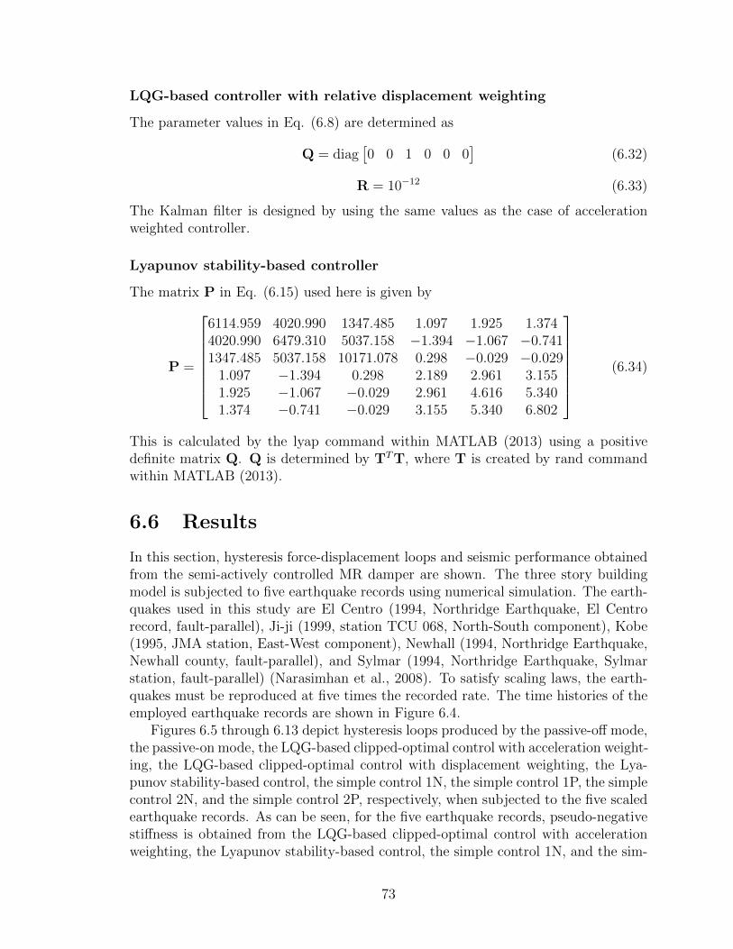
LQG-based controller with relative displacement weighting
The parameter values in Eq. (6.8) are determined as
Q = diag[0 0 1 0 0 0
](6.32)
R = 10−12 (6.33)
The Kalman filter is designed by using the same values as the case of accelerationweighted controller.
Lyapunov stability-based controller
The matrix P in Eq. (6.15) used here is given by
P =
6114.959 4020.990 1347.485 1.097 1.925 1.3744020.990 6479.310 5037.158 −1.394 −1.067 −0.7411347.485 5037.158 10171.078 0.298 −0.029 −0.029
1.097 −1.394 0.298 2.189 2.961 3.1551.925 −1.067 −0.029 2.961 4.616 5.3401.374 −0.741 −0.029 3.155 5.340 6.802
(6.34)
This is calculated by the lyap command within MATLAB (2013) using a positivedefinite matrix Q. Q is determined by TTT, where T is created by rand commandwithin MATLAB (2013).
6.6 Results
In this section, hysteresis force-displacement loops and seismic performance obtainedfrom the semi-actively controlled MR damper are shown. The three story buildingmodel is subjected to five earthquake records using numerical simulation. The earth-quakes used in this study are El Centro (1994, Northridge Earthquake, El Centrorecord, fault-parallel), Ji-ji (1999, station TCU 068, North-South component), Kobe(1995, JMA station, East-West component), Newhall (1994, Northridge Earthquake,Newhall county, fault-parallel), and Sylmar (1994, Northridge Earthquake, Sylmarstation, fault-parallel) (Narasimhan et al., 2008). To satisfy scaling laws, the earth-quakes must be reproduced at five times the recorded rate. The time histories of theemployed earthquake records are shown in Figure 6.4.
Figures 6.5 through 6.13 depict hysteresis loops produced by the passive-off mode,the passive-on mode, the LQG-based clipped-optimal control with acceleration weight-ing, the LQG-based clipped-optimal control with displacement weighting, the Lya-punov stability-based control, the simple control 1N, the simple control 1P, the simplecontrol 2N, and the simple control 2P, respectively, when subjected to the five scaledearthquake records. As can be seen, for the five earthquake records, pseudo-negativestiffness is obtained from the LQG-based clipped-optimal control with accelerationweighting, the Lyapunov stability-based control, the simple control 1N, and the sim-
73

0 2 4 60.5
0
0.5
Time (sec)
Acc
eler
atio
n (
g)
El Centro
0 2 4 60.5
0
0.5
Time (sec)
Acc
eler
atio
n (
g)
Ji ji
0 2 4 61
0
1
Time (sec)
Acc
eler
atio
n (
g)
Kobe
0 2 4 61
0
1
Time (sec)
Acc
eler
atio
n (
g)
Newhall
0 2 4 61
0
1
Time (sec)
Acc
eler
atio
n (
g)
Sylmar
Figure 6.4: Scaled earthquake records
ple control 2N, while, positive stiffness is found in the LQG-based clipped-optimalcontrol with displacement weighting, the simple control 1P, and the simple control2P. These results show that the proposed algorithms can produce various types ofhysteresis control force loops as expected.
Tables 6.1 through 6.5 summarize the peak and RMS values of response rela-tive displacements and absolute accelerations of each floor for the semi-active con-trollers including the LQG-based clipped-optimal control with acceleration weighting,the LQG-based clipped-optimal control with displacement weighting, the Lyapunovstability-based control, the simple control 1N, the simple control 1P, the simple control2N, the simple control 2N. In addition to these semi-active controllers, uncontrolled(i.e., no MR damper), passive-off (the input current to the MR damper is 0), andpassive-on (the input current to the MR damper is 2.0 A) cases are included in thesetables for comparisons. Figures 6.15 and 6.16 compare the ratios to the uncontrolledcase of the peak and RMS relative displacements of the third floor for each controller.The RMS value of n data {p1, p2, · · · pn} is defined as
pRMS =
√∑nk=1 p
2k
n(6.35)
The comparisons of the absolute acceleration of the third floor can be found in Figures6.17 and 6.18. As can be seen in these tables and figures, in general, the semi-activecontrollers producing pseudo-negative stiffness, i.e., the LQG-based clipped-optimalcontrol with acceleration weighting, the simple control 1N, and the simple control 2N
74
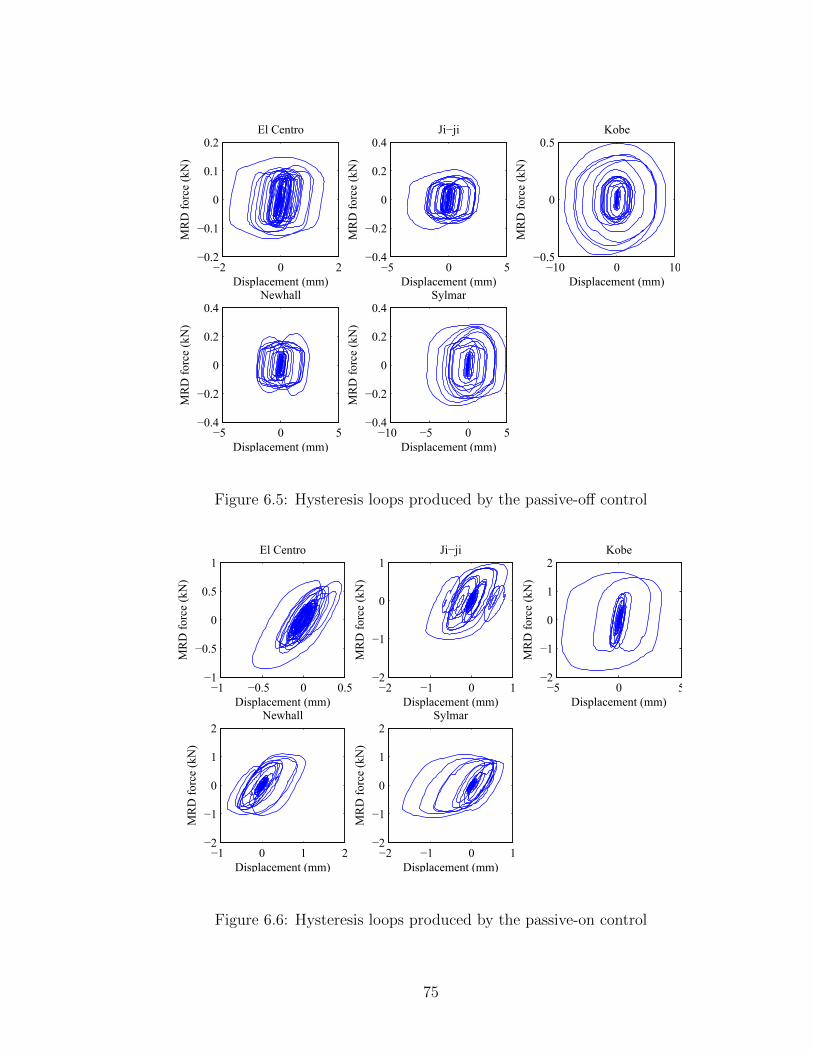
−2 0 2−0.2
−0.1
0
0.1
0.2
Displacement (mm)
MR
D f
orc
e (k
N)
El Centro
−5 0 5−0.4
−0.2
0
0.2
0.4
Displacement (mm)
MR
D f
orc
e (k
N)
Ji−ji
−10 0 10−0.5
0
0.5
Displacement (mm)
MR
D f
orc
e (k
N)
Kobe
−5 0 5−0.4
−0.2
0
0.2
0.4
Displacement (mm)
MR
D f
orc
e (k
N)
Newhall
−10 −5 0 5−0.4
−0.2
0
0.2
0.4
Displacement (mm)
MR
D f
orc
e (k
N)
Sylmar
Figure 6.5: Hysteresis loops produced by the passive-off control
−1 −0.5 0 0.5−1
−0.5
0
0.5
1
Displacement (mm)
MR
D f
orc
e (k
N)
El Centro
−2 −1 0 1−2
−1
0
1
Displacement (mm)
MR
D f
orc
e (k
N)
Ji−ji
−5 0 5−2
−1
0
1
2
Displacement (mm)
MR
D f
orc
e (k
N)
Kobe
−1 0 1 2−2
−1
0
1
2
Displacement (mm)
MR
D f
orc
e (k
N)
Newhall
−2 −1 0 1−2
−1
0
1
2
Displacement (mm)
MR
D f
orc
e (k
N)
Sylmar
Figure 6.6: Hysteresis loops produced by the passive-on control
75
−2 0 2−1
−0.5
0
0.5
Displacement (mm)
MR
D f
orc
e (k
N)
El Centro
−5 0 5−1
−0.5
0
0.5
1
Displacement (mm)
MR
D f
orc
e (k
N)
Ji−ji
−10 −5 0 5−2
−1
0
1
2
Displacement (mm)
MR
D f
orc
e (k
N)
Kobe
−2 0 2−1
−0.5
0
0.5
1
Displacement (mm)
MR
D f
orc
e (k
N)
Newhall
−4 −2 0 2−1
−0.5
0
0.5
1
Displacement (mm)
MR
D f
orc
e (k
N)
Sylmar
Figure 6.7: Hysteresis loops produced by the LQG-based clipped-optimal control withacceleration weighting
−2 0 2−0.5
0
0.5
Displacement (mm)
MR
D f
orc
e (k
N)
El Centro
−5 0 5−1
−0.5
0
0.5
1
Displacement (mm)
MR
D f
orc
e (k
N)
Ji−ji
−10 0 10−2
−1
0
1
2
Displacement (mm)
MR
D f
orc
e (k
N)
Kobe
−2 0 2−1
−0.5
0
0.5
1
Displacement (mm)
MR
D f
orc
e (k
N)
Newhall
−5 0 5−1
−0.5
0
0.5
1
Displacement (mm)
MR
D f
orc
e (k
N)
Sylmar
Figure 6.8: Hysteresis loops produced by the LQG-based clipped-optimal control withinter-story drift weighting
76
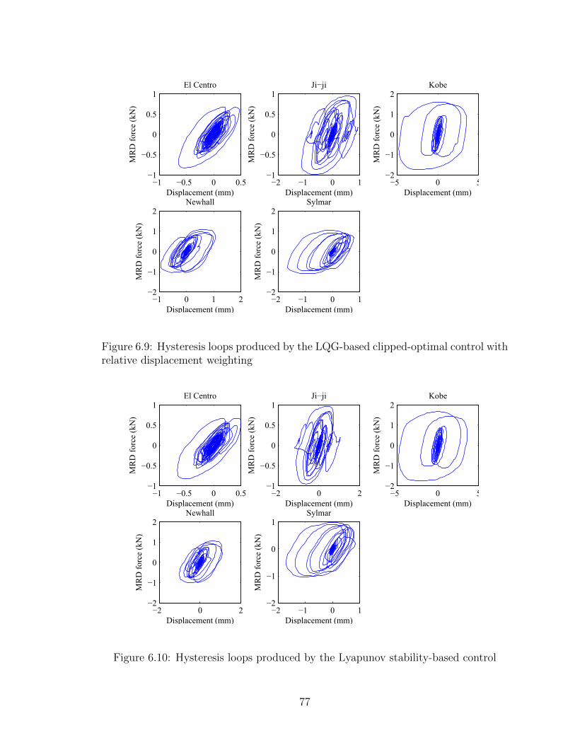
−1 −0.5 0 0.5−1
−0.5
0
0.5
1
Displacement (mm)
MR
D f
orc
e (k
N)
El Centro
−2 −1 0 1−1
−0.5
0
0.5
1
Displacement (mm)
MR
D f
orc
e (k
N)
Ji−ji
−5 0 5−2
−1
0
1
2
Displacement (mm)
MR
D f
orc
e (k
N)
Kobe
−1 0 1 2−2
−1
0
1
2
Displacement (mm)
MR
D f
orc
e (k
N)
Newhall
−2 −1 0 1−2
−1
0
1
2
Displacement (mm)
MR
D f
orc
e (k
N)
Sylmar
Figure 6.9: Hysteresis loops produced by the LQG-based clipped-optimal control withrelative displacement weighting
−1 −0.5 0 0.5−1
−0.5
0
0.5
1
Displacement (mm)
MR
D f
orc
e (k
N)
El Centro
−2 0 2−1
−0.5
0
0.5
1
Displacement (mm)
MR
D f
orc
e (k
N)
Ji−ji
−5 0 5−2
−1
0
1
2
Displacement (mm)
MR
D f
orc
e (k
N)
Kobe
−2 0 2−2
−1
0
1
2
Displacement (mm)
MR
D f
orc
e (k
N)
Newhall
−2 −1 0 1−2
−1
0
1
Displacement (mm)
MR
D f
orc
e (k
N)
Sylmar
Figure 6.10: Hysteresis loops produced by the Lyapunov stability-based control
77

−1 0 1−1
−0.5
0
0.5
1
Displacement (mm)
MR
D f
orc
e (k
N)
El Centro
−2 0 2−2
−1
0
1
Displacement (mm)
MR
D f
orc
e (k
N)
Ji−ji
−10 −5 0 5−2
−1
0
1
2
Displacement (mm)
MR
D f
orc
e (k
N)
Kobe
−2 0 2−1
0
1
2
Displacement (mm)
MR
D f
orc
e (k
N)
Newhall
−4 −2 0 2−2
−1
0
1
2
Displacement (mm)
MR
D f
orc
e (k
N)
Sylmar
Figure 6.11: Hysteresis loops produced by the simple control 1N by Eq. (6.18)
−1 0 1−1
−0.5
0
0.5
1
Displacement (mm)
MR
D f
orc
e (k
N)
El Centro
−2 0 2−1
−0.5
0
0.5
1
Displacement (mm)
MR
D f
orc
e (k
N)
Ji−ji
−10 −5 0 5−2
−1
0
1
2
Displacement (mm)
MR
D f
orc
e (k
N)
Kobe
−2 0 2−1
−0.5
0
0.5
1
Displacement (mm)
MR
D f
orc
e (k
N)
Newhall
−5 0 5−2
−1
0
1
Displacement (mm)
MR
D f
orc
e (k
N)
Sylmar
Figure 6.12: Hysteresis loops produced by the simple control 1P by Eq. (6.19)
78
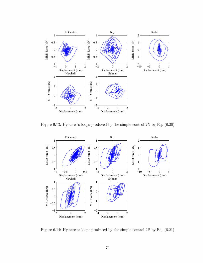
−1 0 1 2−1
−0.5
0
0.5
1
Displacement (mm)
MR
D f
orc
e (k
N)
El Centro
−2 0 2−1
−0.5
0
0.5
1
Displacement (mm)
MR
D f
orc
e (k
N)
Ji−ji
−10 −5 0 5−2
−1
0
1
2
Displacement (mm)
MR
D f
orc
e (k
N)
Kobe
−2 0 2−1
0
1
2
Displacement (mm)
MR
D f
orc
e (k
N)
Newhall
−4 −2 0 2−2
−1
0
1
2
Displacement (mm)
MR
D f
orc
e (k
N)
Sylmar
Figure 6.13: Hysteresis loops produced by the simple control 2N by Eq. (6.20)
−1 −0.5 0 0.5−1
−0.5
0
0.5
1
Displacement (mm)
MR
D f
orc
e (k
N)
El Centro
−2 0 2−1
−0.5
0
0.5
1
Displacement (mm)
MR
D f
orc
e (k
N)
Ji−ji
−10 −5 0 5−2
−1
0
1
2
Displacement (mm)
MR
D f
orc
e (k
N)
Kobe
−2 0 2−1
−0.5
0
0.5
1
Displacement (mm)
MR
D f
orc
e (k
N)
Newhall
−4 −2 0 2−2
−1
0
1
Displacement (mm)
MR
D f
orc
e (k
N)
Sylmar
Figure 6.14: Hysteresis loops produced by the simple control 2P by Eq. (6.21)
79

Table 6.1: Comparisons of peak and RMS values to El Centro earthquake
Displacement (mm) Acceleration (g) Force (N)Controller x1 x2 x3 xa,1 xa,2 xa,3 fMR
Pea
k
Uncontrolled 3.372 5.199 6.073 5.242 6.660 7.498 N/APassive-off 1.775 2.821 3.459 2.759 3.870 4.453 148.2Passive-on 0.616 1.831 2.492 2.673 4.303 4.753 850.1LQG w/ A. 1.272 1.946 2.481 3.569 5.213 4.925 597.1
LQG w/ I.D. 1.474 2.338 2.758 3.300 5.528 4.651 421.3LQG w/ R.D. 0.647 1.858 2.493 2.766 4.723 4.834 823.8
Laypunov 0.666 1.874 2.533 2.998 4.870 4.829 826.9Simple control 1N 0.947 1.634 2.315 4.324 4.371 5.497 811.2Simple control 1P 0.907 2.224 2.840 4.840 5.842 5.677 723.8Simple control 2N 1.181 1.843 2.380 3.526 4.368 5.390 830.2Simple control 2P 0.705 1.928 2.513 2.904 4.617 4.807 782.4
RM
S
Uncontrolled 1.375 2.177 2.618 1.835 2.571 3.141 N/APassive-off 0.367 0.604 0.739 0.715 0.840 1.043 58.4Passive-on 0.124 0.474 0.690 0.626 1.196 1.583 225.8LQG w/ A. 0.213 0.388 0.503 0.828 0.999 1.078 128.7
LQG w/ I.D. 0.251 0.424 0.531 0.807 0.890 0.983 103.0LQG w/ R.D. 0.132 0.473 0.683 0.679 1.239 1.572 217.8
Laypunov 0.136 0.459 0.656 0.735 1.301 1.542 206.9Simple control 1N 0.181 0.384 0.523 0.761 1.019 1.177 166.2Simple control 1P 0.173 0.489 0.681 0.796 1.260 1.493 189.5Simple control 2N 0.222 0.411 0.544 0.784 1.026 1.169 168.5Simple control 2P 0.136 0.482 0.692 0.666 1.211 1.562 216.2
show better performance in reducing both response displacements and accelerations,although some exceptions can be found. In particular, negative stiffness is effectiveat reducing response acceleration. Evaluating the results given in the tables andfigures, the proposed two algorithms producing pseudo-negative stiffness, i.e., thesimple control 1N and the simple control 2N show performance comparable to theLQG-based clipped-optimal controller, or even better results for some cases.
80

Table 6.2: Comparisons of peak and RMS values to Ji-ji earthquake
Displacement (mm) Acceleration (g) Force (N)Controller x1 x2 x3 xa,1 xa,2 xa,3 fMR
Pea
k
Uncontrolled 5.010 7.957 9.593 6.913 9.449 12.070 N/APassive-off 3.562 5.552 6.588 6.505 7.220 8.316 208.2Passive-on 1.099 2.473 3.228 4.736 6.308 6.327 1011.5LQG w/ A. 2.459 3.594 4.479 7.064 6.033 6.868 964.7
LQG w/ I.D. 2.861 4.448 5.594 5.635 7.302 7.986 744.7LQG w/ R.D. 1.139 2.514 3.290 4.742 5.841 5.906 992.4
Laypunov 1.191 2.389 3.201 4.478 6.241 5.776 964.8Simple control 1N 1.598 2.348 2.896 5.470 6.334 6.536 1008.7Simple control 1P 1.795 3.583 4.700 6.626 7.957 8.679 893.2Simple control 2N 1.722 2.490 2.880 5.608 5.668 6.841 951.5Simple control 2P 1.703 3.347 4.247 6.703 7.858 7.803 953.6
RM
S
Uncontrolled 2.149 3.397 4.077 2.733 3.984 4.784 N/APassive-off 0.838 1.328 1.594 1.287 1.629 1.926 78.2Passive-on 0.301 0.713 0.971 0.918 1.472 1.910 298.8LQG w/ A. 0.584 0.876 1.050 1.259 1.325 1.532 200.5
LQG w/ I.D. 0.664 1.005 1.197 1.333 1.380 1.588 162.6LQG w/ R.D. 0.328 0.728 0.978 0.961 1.446 1.859 282.4
Laypunov 0.340 0.724 0.966 0.968 1.450 1.822 279.4Simple control 1N 0.470 0.755 0.943 1.055 1.353 1.577 269.0Simple control 1P 0.408 0.845 1.099 1.283 1.657 1.955 241.5Simple control 2N 0.474 0.767 0.958 1.061 1.370 1.608 263.5Simple control 2P 0.369 0.778 1.022 1.152 1.588 1.888 252.0
81
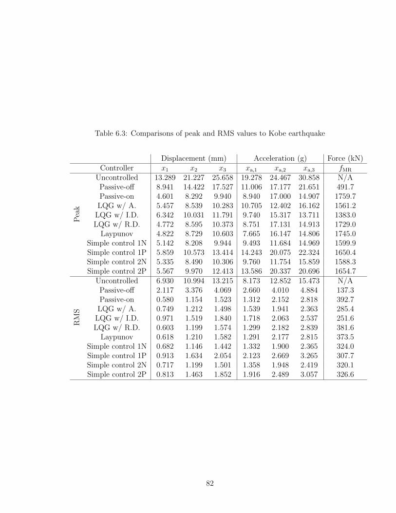
Table 6.3: Comparisons of peak and RMS values to Kobe earthquake
Displacement (mm) Acceleration (g) Force (kN)Controller x1 x2 x3 xa,1 xa,2 xa,3 fMR
Pea
k
Uncontrolled 13.289 21.227 25.658 19.278 24.467 30.858 N/APassive-off 8.941 14.422 17.527 11.006 17.177 21.651 491.7Passive-on 4.601 8.292 9.940 8.940 17.000 14.907 1759.7LQG w/ A. 5.457 8.539 10.283 10.705 12.402 16.162 1561.2
LQG w/ I.D. 6.342 10.031 11.791 9.740 15.317 13.711 1383.0LQG w/ R.D. 4.772 8.595 10.373 8.751 17.131 14.913 1729.0
Laypunov 4.822 8.729 10.603 7.665 16.147 14.806 1745.0Simple control 1N 5.142 8.208 9.944 9.493 11.684 14.969 1599.9Simple control 1P 5.859 10.573 13.414 14.243 20.075 22.324 1650.4Simple control 2N 5.335 8.490 10.306 9.760 11.754 15.859 1588.3Simple control 2P 5.567 9.970 12.413 13.586 20.337 20.696 1654.7
RM
S
Uncontrolled 6.930 10.994 13.215 8.173 12.852 15.473 N/APassive-off 2.117 3.376 4.069 2.660 4.010 4.884 137.3Passive-on 0.580 1.154 1.523 1.312 2.152 2.818 392.7LQG w/ A. 0.749 1.212 1.498 1.539 1.941 2.363 285.4
LQG w/ I.D. 0.971 1.519 1.840 1.718 2.063 2.537 251.6LQG w/ R.D. 0.603 1.199 1.574 1.299 2.182 2.839 381.6
Laypunov 0.618 1.210 1.582 1.291 2.177 2.815 373.5Simple control 1N 0.682 1.146 1.442 1.332 1.900 2.365 324.0Simple control 1P 0.913 1.634 2.054 2.123 2.669 3.265 307.7Simple control 2N 0.717 1.199 1.501 1.358 1.948 2.419 320.1Simple control 2P 0.813 1.463 1.852 1.916 2.489 3.057 326.6
82
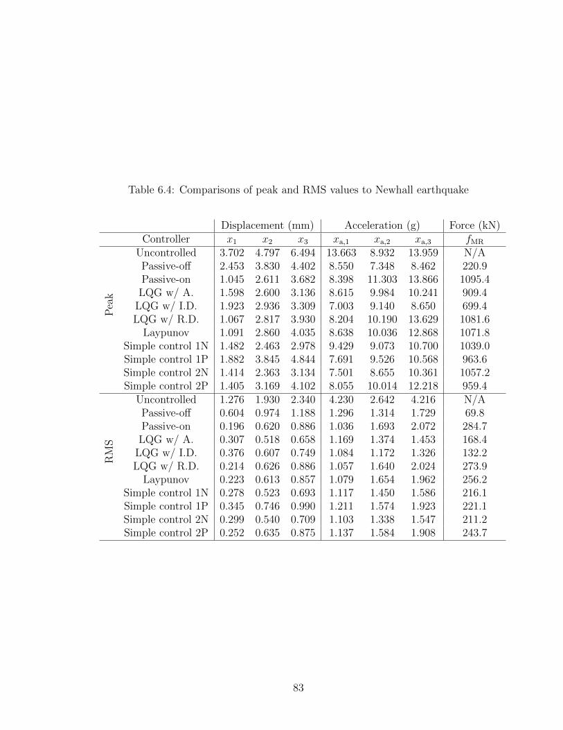
Table 6.4: Comparisons of peak and RMS values to Newhall earthquake
Displacement (mm) Acceleration (g) Force (kN)Controller x1 x2 x3 xa,1 xa,2 xa,3 fMR
Pea
k
Uncontrolled 3.702 4.797 6.494 13.663 8.932 13.959 N/APassive-off 2.453 3.830 4.402 8.550 7.348 8.462 220.9Passive-on 1.045 2.611 3.682 8.398 11.303 13.866 1095.4LQG w/ A. 1.598 2.600 3.136 8.615 9.984 10.241 909.4
LQG w/ I.D. 1.923 2.936 3.309 7.003 9.140 8.650 699.4LQG w/ R.D. 1.067 2.817 3.930 8.204 10.190 13.629 1081.6
Laypunov 1.091 2.860 4.035 8.638 10.036 12.868 1071.8Simple control 1N 1.482 2.463 2.978 9.429 9.073 10.700 1039.0Simple control 1P 1.882 3.845 4.844 7.691 9.526 10.568 963.6Simple control 2N 1.414 2.363 3.134 7.501 8.655 10.361 1057.2Simple control 2P 1.405 3.169 4.102 8.055 10.014 12.218 959.4
RM
S
Uncontrolled 1.276 1.930 2.340 4.230 2.642 4.216 N/APassive-off 0.604 0.974 1.188 1.296 1.314 1.729 69.8Passive-on 0.196 0.620 0.886 1.036 1.693 2.072 284.7LQG w/ A. 0.307 0.518 0.658 1.169 1.374 1.453 168.4
LQG w/ I.D. 0.376 0.607 0.749 1.084 1.172 1.326 132.2LQG w/ R.D. 0.214 0.626 0.886 1.057 1.640 2.024 273.9
Laypunov 0.223 0.613 0.857 1.079 1.654 1.962 256.2Simple control 1N 0.278 0.523 0.693 1.117 1.450 1.586 216.1Simple control 1P 0.345 0.746 0.990 1.211 1.574 1.923 221.1Simple control 2N 0.299 0.540 0.709 1.103 1.338 1.547 211.2Simple control 2P 0.252 0.635 0.875 1.137 1.584 1.908 243.7
83

Table 6.5: Comparisons of peak and RMS values to Sylmar earthquake
Displacement (mm) Acceleration (g) Force (kN)Controller x1 x2 x3 xa,1 xa,2 xa,3 fMR
Pea
k
Uncontrolled 8.128 12.445 14.470 12.816 16.097 17.079 N/APassive-off 5.325 8.371 9.948 7.535 10.549 11.145 285.5Passive-on 1.668 3.761 5.521 5.958 8.338 13.856 1118.9LQG w/ A. 3.161 4.708 5.163 6.996 8.952 9.658 939.0
LQG w/ I.D. 3.481 5.339 6.239 6.620 9.448 8.188 809.8LQG w/ R.D. 1.651 3.737 5.485 5.645 8.347 13.772 1097.9
Laypunov 1.715 3.758 5.420 5.731 7.791 13.179 1032.9Simple control 1N 2.492 3.759 4.534 7.114 6.662 10.658 1148.9Simple control 1P 2.736 5.325 6.920 8.897 10.091 11.747 1037.4Simple control 2N 2.496 3.698 4.805 6.812 6.957 10.157 1095.8Simple control 2P 2.207 4.415 5.535 7.769 9.689 13.067 1068.5
RM
S
Uncontrolled 3.750 5.948 7.151 4.662 6.979 8.475 N/APassive-off 1.180 1.891 2.285 1.577 2.284 2.822 93.9Passive-on 0.240 0.688 0.975 0.894 1.593 2.132 298.6LQG w/ A. 0.479 0.736 0.901 1.170 1.220 1.494 185.7
LQG w/ I.D. 0.562 0.880 1.069 1.097 1.251 1.532 155.8LQG w/ R.D. 0.248 0.690 0.973 0.866 1.532 2.082 288.6
Laypunov 0.266 0.693 0.965 0.877 1.462 2.004 275.0Simple control 1N 0.404 0.682 0.875 1.048 1.317 1.655 244.3Simple control 1P 0.485 0.938 1.209 1.412 1.764 2.163 220.8Simple control 2N 0.418 0.706 0.901 1.025 1.328 1.652 235.2Simple control 2P 0.377 0.800 1.064 1.248 1.742 2.120 251.2
84

El
Cen
tro
Jiji
Kobe
New
hal
lS
ylm
ar0
20
40
60
80
100
Ratio to uncontrolled (%)
P.
off
P.
on
LQ
G (
A.)
LQ
G (
I.D
.)
LQ
G (
R.D
.)
Lyap
unov
S.C
. 1N
S.C
. 1P
S.C
. 2N
S.C
. 2P
Fig
ure
6.15
:C
ompar
ison
sof
the
pea
kre
spon
sedis
pla
cem
ents
of3r
dfloor
El
Cen
tro
Jiji
Kobe
New
hal
lS
ylm
ar0
20
40
60
80
100
Ratio to uncontrolled (%)
P.
off
P.
on
LQ
G (
A.)
LQ
G (
I.D
.)
LQ
G (
R.D
.)
Lyap
unov
S.C
. 1N
S.C
. 1P
S.C
. 2N
S.C
. 2P
Fig
ure
6.16
:C
ompar
ison
sof
the
RM
Sre
spon
sedis
pla
cem
ents
of3r
dfloor
85

El
Cen
tro
Jiji
Kobe
New
hal
lS
ylm
ar0
20
40
60
80
100
Ratio to uncontrolled (%)
P.
off
P.
on
LQ
G (
A.)
LQ
G (
I.D
.)
LQ
G (
R.D
.)
Lyap
unov
S.C
. 1N
S.C
. 1P
S.C
. 2N
S.C
. 2P
Fig
ure
6.17
:C
ompar
ison
sof
the
pea
kre
spon
seac
cele
rati
ons
of3r
dfloor
El
Cen
tro
Jiji
Kobe
New
hal
lS
ylm
ar0
20
40
60
80
100
Ratio to uncontrolled (%)
P.
off
P.
on
LQ
G (
A.)
LQ
G (
I.D
.)
LQ
G (
R.D
.)
Lyap
unov
S.C
. 1N
S.C
. 1P
S.C
. 2N
S.C
. 2P
Fig
ure
6.18
:C
ompar
ison
sof
the
RM
Sre
spon
seac
cele
rati
ons
of3r
dfloor
86

Figure 6.19 shows the earthquake input energies into the building model forthree semi-active controllers producing pseudo-negative stiffness, i.e., the LQG-basedclipped-optimal control with acceleration weighting, the simple control 1N, and thesimple control 2N. The earthquake input energy Ei is defined as (Chopra, 2007)
Ei = −∫ t
0
xTMsLsxgdτ (6.36)
As can be seen in the figure, the simple controls 1N and 2N can reduce input earth-quake energy more than the LQG-based clipped-optimal control applied to El Centro,Ji-ji, and Kobe earthquake records. Even for Newhall and Sylmar records, the energyabsorption capabilities of the proposed two simple controllers are comparable to theLQG-based clipped-optimal control case.
6.7 Summary
This chapter proposed two new model-free semi-active control algorithms for control-lable dampers. One of the algorithms needs only the directions of the displacementand the velocity of the damper to decide the property of the damper. The otherneeds the directions of only the displacement and the output force of the damper.Thus, the structure model and a number of sensors are not required to implement theproposed algorithms. Moreover, this research showed that the proposed controllerscan produce versatile hysteresis control force loops through numerical simulations onthe scaled three-story building model with a MR damper. Also, the effectiveness ofhysteresis loops having negative stiffness was verified. Additionally, the numericalresults showed that the proposed two algorithms producing pseudo-negative stiffnesshad performance comparable to the LQG-based clipped-optimal controllers, whichneed the accurate structure model and more sensors.
87

0 2 4 60
1
2
3
4
5
Time (sec)
Input
ener
gy (
N⋅m
)El Centro
LQG (A.)
LQG (I.D.)
S.C.1N
S.C.2N
0 2 4 60
5
10
15
Time (sec)
Input
ener
gy (
N⋅m
)
Ji ji
LQG (A.)
LQG (I.D.)
S.C.1N
S.C.2N
0 2 4 60
10
20
30
40
50
Time (sec)
Input
ener
gy (
N⋅m
)
Kobe
LQG (A.)
LQG (I.D.)
S.C.1N
S.C.2N
0 2 4 60
2
4
6
8
10
Time (sec)
Input
ener
gy (
N⋅m
)
Newhall
LQG (A.)
LQG (I.D.)
S.C.1N
S.C.2N
0 2 4 60
5
10
15
Time (sec)
Input
ener
gy (
N⋅m
)
Sylmar
LQG (A.)
LQG (I.D.)
S.C.1N
S.C.2N
Figure 6.19: Comparisons of earthquake input energy
88

Chapter 7
RTHS FOR SEMI-ACTIVE CONTROL ON A
MDOF STRUCTURE
To show the effectiveness of semi-active control strategies, experimental verificationis necessary. However, due to the limitation of cost and facilities, it is not practicalto carry out shaking table testing for full-scale structures. To provide experimentalverification, RTHS is an alternative method where the semi-active control devices canbe experimentally tested, while the remaining components in the structural systemare simultaneously tested through numerical simulation.
Time delays/lags are critical issues in RTHS, so introducing compensation forthem is essential. However, RTHS becomes more challenging for MDOF structuresbecause MDOF structures include significant contributions at different frequencieswhich can not be compensated by assuming a constant time delay. The focus ofthis chapter is to show the accuracy of the model-based compensator for RTHS on aMDOF structure using a smart outrigger damping system.
Smart outrigger damping systems have been proposed as a novel energy dissipa-tion system to protect high-rise buildings from severe earthquakes and strong winds.In these damping systems, devices such as MR dampers are installed vertically be-tween the outrigger and perimeter columns to achieve large and adaptable energydissipation. In this chapter, to complement the high performance shown in previoustheoretical studies, this control approach is experimentally verified as well.
7.1 Smart outrigger damping system
In this section, the models for both the high-rise building and the MR damper arepresented. Also, the semi-active control algorithm selected for the system is illus-trated. In RTHS, a physical MR damper is used, while in numerical simulation, theMR damper model created in Section 4.1 is used.
7.1.1 Problem formulation
Smart outrigger damping systems are an attractive method to achieve sufficient dis-placement for damping devices on high-rise buildings. According to Yang et al.(2004a), a high-rise building can be modeled as a cantilevered beam in which thestructural deformations are derived from the behavior of the core. For a high-risebuilding with outrigger damping, the control devices (e.g., viscous dampers or MRdampers) are located between the outrigger walls and the perimeter columns. Assum-ing that the perimeter columns are axially very stiff and that the outrigger behaves
89

as a rigid body, then the high-rise building with damped outriggers can be modeledas shown in Figure 7.1. As can be seen, the forces from the control devices resultin moments being applied to the core through the rigid outrigger. In essence, thedamped outrigger acts as a point rotational damping device. The moment applied tothe core by the outrigger system fm can be written as
fm = ndoef (7.1)
where f is the force from a single control device; nd is the number of control devices;oe is the distance from the control devices to the center of the core (see Figure 7.1).The equation of motion can be written as
Mu + Cu + Ku = Λfm −MΓxg (7.2)
where M, C, K are the structural mass, damping, stiffness matrices, respectively; uis the structural deformation vector; Λ is an influence vector that applies the damperrestoring force to the appropriate rotational degrees of freedom (DOF); Γ is a vectorwith entries equal to unity for translational DOFs and zero for others; and xg is theground acceleration. The state-space form of Eq. (7.2) is given by
x = Ax + Bfm + Exg (7.3)
y = Cyx + Dyfm + Fyxg + v (7.4)
z = Czx + Dzfm + Fzxg (7.5)
Figure 7.1: Mechanism of outrigger systems
90

where y presents the measured structural responses including the relative displace-ments, the relative velocities, and the absolute floor accelerations; v is the measure-ment noise; and z corresponds to the regulated structural responses. A, B, Cy,Cz, Dy, Dz, E, Fy, and Fz are appropriately chosen matrices corresponding to theassociated state-space equations.
7.1.2 Building model
The building used in this study is the St. Francis Shangri-La Place in the Philippines(Willford et al., 2008; Infanti et al., 2008; Chang et al., 2013). This 60-story buildinghas a height of 210 m and has 12 perimeter columns which are 20 m from the buildingcenterline. The concrete core is assumed to be 12 m × 12 m with 0.5 m thickness. Thetotal mass of the building is 30,000 tons and the outrigger system installed consistsof 16 viscous dampers, 8 of which control the response in each of the two orthogonaldirections.
To create the model for evaluation, a vertical cantilever beam model based on theBernoulli-Euler beam theory is applied. A finite element model is developed so thatevery story has one translational and one rotational degree of freedoms. Therefore,the total number of degrees-of-freedom should be 120 (60 in translation and 60 inrotation). Hence, the reduced structural deformation vector up to mth mode, ured,m,can be represented by
ured,m(t) =m∑i=1
φiqi(t) = Φmqm(t) (7.6)
whereΦm =
[φ1 φ2 · · · φm
](7.7)
is the mode shape matrix up to the mth mode and
qm =[q1 q2 · · · qm
](7.8)
is the modal coordinate vector up to the mth mode. In this study, m = 10 forthe evaluation model (i.e., to perform the response calculations) and m = 5 for thecontrol design model (i.e., to design the semi-active controllers). The first 10 naturalfrequencies are 0.18 Hz, 1.15 Hz, 3.14 Hz, 6.00 Hz, 9.61 Hz, 13.84 Hz, 18.56 Hz, 23.66Hz, 29.06 Hz, and 34.66 Hz, respectively. Damping of 2 % is assumed in each mode.
The 42nd floor is selected as the optimal location of the outrigger and dampers inthis study based on the numerical study of Chang et al. (2013). In this study, to as-sume that the MR dampers installed on the opposite sides behave anti-symmetrically,the displacement of the MR dampers are calculated only from the rotation of the 42ndfloor; i.e. the horizontal translation effect to the displacement of the MR dampers is ig-nored. The magnitudes of the transfer functions for the reduced building model frominput earthquake acceleration to the displacement and acceleration of the damperare shown in Figure 7.2. As can be seen, high-frequency content due to high-moderesponses affects the acceleration significantly.
91

0 10 20 30 40 50
10−6
10−4
10−2
100
Frequency (Hz)
Mag
nit
ude
(a)
0 10 20 30 40 5010
−2
10−1
100
101
Frequency (Hz)
Mag
nit
ude
(b)
Figure 7.2: Transfer functions from input acceleration to the damper; (a) Displace-ment, (b) Acceleration
Note that the estimated damping after the MR dampers are installed to the 42ndfloor are, from the first mode, 4.74 %, 4.77 %, 2.00 %, 3.72 %, 4.03 %, 2.05 %, 3.32%, 4.09 %, 2.17 %, and 2.89 %, respectively. These values are calculated by assumingviscous dampers which have the same level damping as the passive on mode MRdampers.
7.1.3 Semi-active control designs
To facilitate semi-active control using MR dampers, control methods that translatethe required control force into an input current command are typically used. Dykeet al. (1996c) proposed a LQG-based clipped-optimal control method which had beenexperimentally verified using MR dampers and will be selected for this study. Inthis control method, the outrigger system employs the LQG/H2 control algorithm tocalculate the optimal control force. By reconsidering Eq. (7.5), the cost function ofthe LQG/H2 control can be written by
J = limt→∞
1
tE
[∫ t
0
(zTQz +Rfm,c
2)dt
](7.9)
where Q and R are the weighting parameters, fm,c is a control moment, E[·] means theexpected value of the quantity in brackets and t represents the time. By minimizingEq. (7.9), the control force is a function of the structural states. In the LQG/H2
control, the Kalman filter estimates (Nagarajaiah and Narasimhan, 2006) the statebased on the measured responses such that
˙x = Ax + Bfm,c + L (y −Cyx−Dyfm,c) (7.10)
fm,c = −Kcx (7.11)
92
where L is the Kalman gain, Kc is the optimal control gain found by minimizing Eq.(7.9), and x is the estimated state by the Kalman filter. The clipped-optimal controlalgorithms are used to convert the optimal control force of Eq. (7.11) to a commandvoltage for the MR damper. The desired input is given by
id = VmaxH {(fm,c − fm,MR) fm,MR} (7.12)
where H{·} is the Heaviside function, id is the input voltage to a MR damper; Vmax isthe maximum input voltage, fm,c is the desired optimal control moment generated byEq. (7.11) and fm,MR is the actual damping moment generated by the MR damperforce and Eq. (7.1). The clipped-optimal controller logic is illustrated in Figure 6.1.
Four LQG-based clipped-optimal control strategies are created through differentLQG designs and evaluated in this study. Controller #1 focuses on minimizing therelative translational displacements to the ground at the 10th, 20th, 30th, 40th, 50th,and 60th floors in Eq. (7.9), while controller #2 focuses on minimizing the transla-tional absolute floor accelerations at the same locations. In addition, controllers #3and #4 minimize the rotational displacements and accelerations at the same locations,respectively. For the Kalman filter in Eqs. (7.10) and (7.11), this study assumes thatthe absolute translational floor accelerations at the 10th, 20th, 30th, 40th, 50th, and60th floors are available to estimate the required force. The maximum input currentimax in the clipped-optimal control is 2.0 A based on the MR damper specifications.
7.2 Results
To investigate the seismic performance of the smart outrigger system, the resultsobtained from RTHS and numerical simulations are shown. The influence of magni-tude and time delay errors on the results of RTHS is presented. In this section, twoearthquake records are considered: (1) the north-south component of the El Centroearthquake in Imperial Valley, CA in 1940 and (2) the north-south component of theKobe earthquake in Hyogo-ken Nanbu in 1995 (Yoshida and Dyke, 2004).
In this research, an assumption is made that required capacity of the MR damperto the target building can be achieved in both simulation and RTHS as follows: Theoutput force of the MR damper is multiplied by 2500 and the displacement of the MRdamper is scaled such that 1 inch (25.4 mm) in the MR damper corresponds to 0.1 min the model of the outrigger damping system. The peak ground accelerations (PGAs)of input records are normalized to 0.3 g, and 0.5 g for the El Centro earthquake and0.3 g, 0.5 g, and 0.7 g for the Kobe earthquake. The parameters Q and R of each semi-active controller are determined based on the simulation results of 0.3 g El Centrocase by trial and error. These values are selected such that the maximum stroke ofthe physical MR damper is not exceeded. All numerical simulations are performedin SIMULINK (2013). For RTHS, models are created in SIMULINK (2013) andimplemented in the DSP using MATLAB (2013)’s Real-Time Workshop.
93
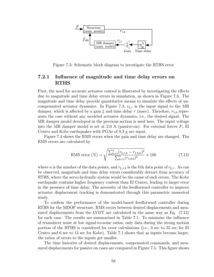
Structure(num. model)
F
MR damper(num. model)
Gain
fMR
Time delay
rξ,τξ τ
r1,0
Figure 7.3: Schematic block diagram to investigate the RTHS error
7.2.1 Influence of magnitude and time delay errors onRTHS
First, the need for accurate actuator control is illustrated by investigating the effectsdue to magnitude and time delay errors in simulation, as shown in Figure 7.3. Themagnitude and time delay provide quantitative means to simulate the effects of un-compensated actuator dynamics. In Figure 7.3, rξ,τ is the input signal to the MRdamper, which is affected by a gain ξ and time delay τ (msec). Therefore, r1,0 repre-sents the case without any modeled actuator dynamics, i.e., the desired signal. TheMR damper model developed in the previous section is used here. The input voltageinto the MR damper model is set at 2.0 A (passive-on). For external forces F , ElCentro and Kobe earthquakes with PGAs of 0.3 g are input.
Figure 7.4 shows the RMS errors when the gain and time delay are changed. TheRMS errors are calculated by
RMS error (%) =
√∑nk=1(rξ,τ,k − r1,0,k)2∑n
k=1(r1,0,k)2
× 100 (7.13)
where n is the number of the data points, and rξ,τ,k is the kth data point of rξ,τ . As canbe observed, magnitude and time delay errors considerably detract from accuracy ofRTHS, where the servo-hydraulic system would be the cause of such errors. The Kobeearthquake contains higher frequency content than El Centro, leading to larger errorin the presence of time delay. The necessity of the feedforward controller to improveactuator displacement tracking is demonstrated through this parametric numericalstudy.
To confirm the performance of the model-based feedforward controller duringRTHS for the MDOF structure, RMS errors between desired displacements and mea-sured displacements from the LVDT are calculated in the same way as Eq. (7.13)for each case. The results are summarized in Table 7.1. To minimize the influenceof transducer noise at low signal-to-noise ratios, only data during the strong motionportion of the RTHS is considered for error calculations (i.e., 3 sec to 35 sec for ElCentro and 6 sec to 13 sec for Kobe). Table 7.1 shows that as inputs become larger,the ratios of errors to the inputs get smaller.
The time histories of desired displacements, compensated commands, and mea-sured displacements for passive on cases are compared in Figure 7.5. This figure shows
94

0
10
20
30
0.98
1
1.02
0
2
4
6
8
10
Time delay (msec)
(a) El Centro (0.3 g)
Gain
RM
S e
rror
(%)
0
10
20
30
0.98
1
1.02
0
2
4
6
8
10
Time delay (msec)
(b) Kobe (0.3 g)
Gain
RM
S e
rror
(%)
0
1
2
3
4
5
6
7
8
9
10
Figure 7.4: RMS errors generated by gain and time delay errors; (a) El Centro (0.3g), (b) Kobe (0.3 g)
Table 7.1: RMS errors for each test (%)
Input Passive LQG #1 LQG #2 LQG #3 LQG #4El Centro (0.3 g) 1.945 2.196 2.333 2.097 2.009El Centro (0.5 g) 1.418 1.263 1.342 1.323 1.282
Kobe (0.3 g) 2.423 3.358 2.848 2.646 2.965Kobe (0.5 g) 1.244 1.846 1.517 1.314 1.569Kobe (0.7 g) 0.929 1.323 1.057 1.022 1.102
that the feedforward controller makes the compensated commands lead the desireddisplacements by more than 20 msec. Also, the power spectral densities of commandinputs are plotted in Figure 7.6 to investigate the influence of high-frequency com-mands to the servo-hydraulic system due to high-mode responses. As can be seen,peaks appear around natural frequency of each mode even in the high-frequencyrange. Also, this figure shows that Kobe cases need a more effective compensator inthe high-frequency range for RTHS than El Centro cases.
7.2.2 Experimental assessment
For structural control performance evaluation, the structural control design is pri-marily aimed at reducing relative displacements and base shear forces, which are themajor indicators of the performance of a structure. In addition to the semi-activecontrol strategies, the outrigger damping system with passive-on mode (i.e., constant
95

(a)
(b)
0 5 10 15 20 25 30 35 40 45
−5
0
5
Time (sec)
Dis
p. (m
m)
6 6.02 6.04 6.06 6.08 6.1 6.12 6.14 6.16 6.18 6.2
3
4
5
Time (sec)
Dis
p. (m
m)
Desired
Command
Measured
0 5 10 15 20 25 30 35 40 45
−5
0
5
Time (sec)
Dis
p. (m
m)
6.95 7 7.05 7.1 7.15
3
4
5
Time (sec)
Dis
p. (m
m)
Desired
Command
Measured
Figure 7.5: Comparisons between measured and command displacements for passive-on case; (a) El Centro (0.3 g), (b) Kobe (0.3 g)
current) MR dampers and the performance of the uncontrolled (bare) building arealso considered.
The time histories of the MR damper forces, the relationships between the dis-placements and the forces, and between the velocities and forces subjected to El Ceon-tro and Kobe earthquakes whose PGAs are scaled to 0.3 g are depicted in Figures 7.7through 7.24. Figures 7.7 through 7.11 and Figures 7.16 through 7.20 compares theMR damper forces obtained from numerical simulation and RTHS produced by thepassive-on, the LQG-based clipped-optimal controllers #1, #2, #3, and #4. Thesefigures show that the proposed MR damper model created by the phenomenologicalmodel simulates the physical MR damper very well in both passive and semi-activecases. However, slight discrepancies can be observed. These differences between thesimulation and the experimental results demonstrate the need for RTHS to assessthe performance of advanced damping systems. It should be noted that the expectedproperties of the hysteresis loops can not be found in any LQG-based clipped optimalcontrollers.
96
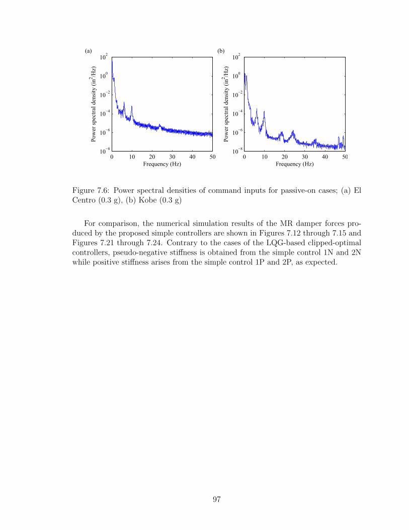
0 10 20 30 40 5010
−8
10−6
10−4
10−2
100
102
Frequency (Hz)
Pow
er s
pec
tral
den
sity
(in
2/H
z)
(a)
0 10 20 30 40 5010
−8
10−6
10−4
10−2
100
102
Frequency (Hz)
Pow
er s
pec
tral
den
sity
(in
2/H
z)
(b)
Figure 7.6: Power spectral densities of command inputs for passive-on cases; (a) ElCentro (0.3 g), (b) Kobe (0.3 g)
For comparison, the numerical simulation results of the MR damper forces pro-duced by the proposed simple controllers are shown in Figures 7.12 through 7.15 andFigures 7.21 through 7.24. Contrary to the cases of the LQG-based clipped-optimalcontrollers, pseudo-negative stiffness is obtained from the simple control 1N and 2Nwhile positive stiffness arises from the simple control 1P and 2P, as expected.
97
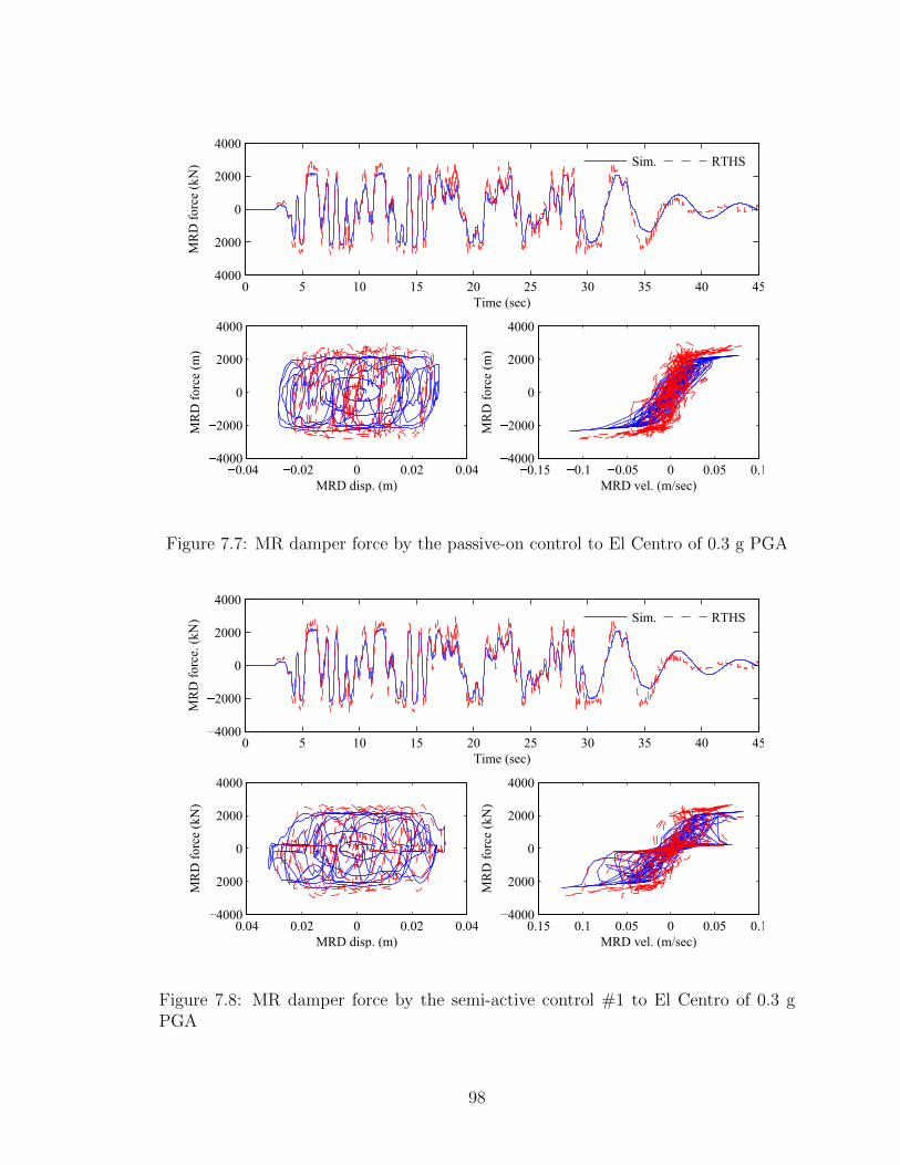
0 5 10 15 20 25 30 35 40 454000
2000
0
2000
4000
Time (sec)
MR
D f
orc
e (k
N) Sim. RTHS
0.04 0.02 0 0.02 0.044000
2000
0
2000
4000
MRD disp. (m)
MR
D f
orc
e (m
)
0.15 0.1 0.05 0 0.05 0.14000
2000
0
2000
4000
MRD vel. (m/sec)M
RD
forc
e (m
)
Figure 7.7: MR damper force by the passive-on control to El Centro of 0.3 g PGA
0 5 10 15 20 25 30 35 40 454000
2000
0
2000
4000
Time (sec)
MR
D f
orc
e. (
kN
) Sim. RTHS
0.04 0.02 0 0.02 0.044000
2000
0
2000
4000
MRD disp. (m)
MR
D f
orc
e (k
N)
0.15 0.1 0.05 0 0.05 0.14000
2000
0
2000
4000
MRD vel. (m/sec)
MR
D f
orc
e (k
N)
Figure 7.8: MR damper force by the semi-active control #1 to El Centro of 0.3 gPGA
98
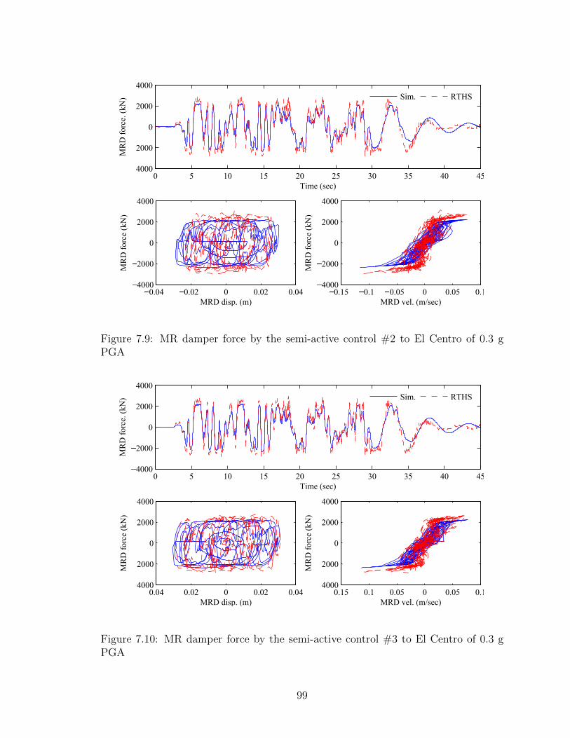
0 5 10 15 20 25 30 35 40 454000
2000
0
2000
4000
Time (sec)
MR
D f
orc
e. (
kN
) Sim. RTHS
0.04 0.02 0 0.02 0.044000
2000
0
2000
4000
MRD disp. (m)
MR
D f
orc
e (k
N)
0.15 0.1 0.05 0 0.05 0.14000
2000
0
2000
4000
MRD vel. (m/sec)M
RD
forc
e (k
N)
Figure 7.9: MR damper force by the semi-active control #2 to El Centro of 0.3 gPGA
0 5 10 15 20 25 30 35 40 454000
2000
0
2000
4000
Time (sec)
MR
D f
orc
e. (
kN
) Sim. RTHS
0.04 0.02 0 0.02 0.044000
2000
0
2000
4000
MRD disp. (m)
MR
D f
orc
e (k
N)
0.15 0.1 0.05 0 0.05 0.14000
2000
0
2000
4000
MRD vel. (m/sec)
MR
D f
orc
e (k
N)
Figure 7.10: MR damper force by the semi-active control #3 to El Centro of 0.3 gPGA
99
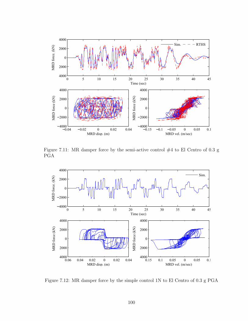
0 5 10 15 20 25 30 35 40 454000
2000
0
2000
4000
Time (sec)
MR
D f
orc
e. (
kN
) Sim. RTHS
0.04 0.02 0 0.02 0.044000
2000
0
2000
4000
MRD disp. (m)
MR
D f
orc
e (k
N)
0.15 0.1 0.05 0 0.05 0.14000
2000
0
2000
4000
MRD vel. (m/sec)M
RD
forc
e (k
N)
Figure 7.11: MR damper force by the semi-active control #4 to El Centro of 0.3 gPGA
0 5 10 15 20 25 30 35 40 454000
2000
0
2000
4000
Time (sec)
MR
D f
orc
e. (
kN
) Sim.
0.06 0.04 0.02 0 0.02 0.044000
2000
0
2000
4000
MRD disp. (m)
MR
D f
orc
e (k
N)
0.15 0.1 0.05 0 0.05 0.14000
2000
0
2000
4000
MRD vel. (m/sec)
MR
D f
orc
e (k
N)
Figure 7.12: MR damper force by the simple control 1N to El Centro of 0.3 g PGA
100
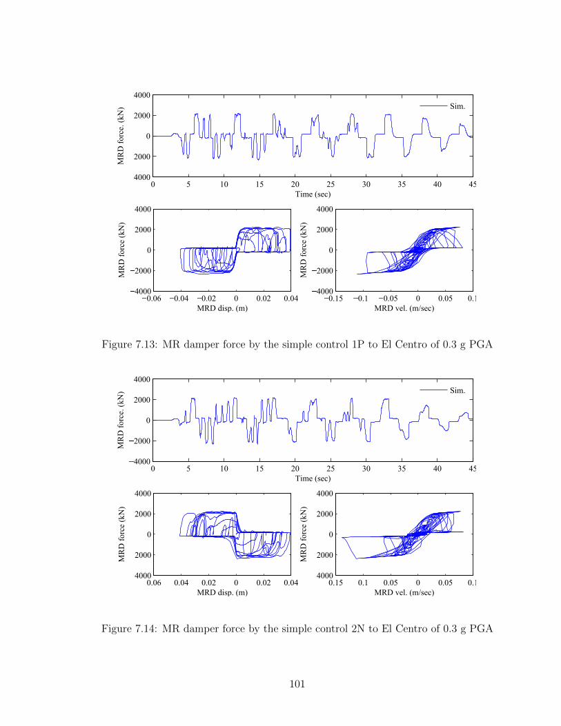
0 5 10 15 20 25 30 35 40 454000
2000
0
2000
4000
Time (sec)
MR
D f
orc
e. (
kN
) Sim.
0.06 0.04 0.02 0 0.02 0.044000
2000
0
2000
4000
MRD disp. (m)
MR
D f
orc
e (k
N)
0.15 0.1 0.05 0 0.05 0.14000
2000
0
2000
4000
MRD vel. (m/sec)M
RD
forc
e (k
N)
Figure 7.13: MR damper force by the simple control 1P to El Centro of 0.3 g PGA
0 5 10 15 20 25 30 35 40 454000
2000
0
2000
4000
Time (sec)
MR
D f
orc
e. (
kN
) Sim.
0.06 0.04 0.02 0 0.02 0.044000
2000
0
2000
4000
MRD disp. (m)
MR
D f
orc
e (k
N)
0.15 0.1 0.05 0 0.05 0.14000
2000
0
2000
4000
MRD vel. (m/sec)
MR
D f
orc
e (k
N)
Figure 7.14: MR damper force by the simple control 2N to El Centro of 0.3 g PGA
101

0 5 10 15 20 25 30 35 40 454000
2000
0
2000
4000
Time (sec)
MR
D f
orc
e. (
kN
) Sim.
0.06 0.04 0.02 0 0.02 0.044000
2000
0
2000
4000
MRD disp. (m)
MR
D f
orc
e (k
N)
0.15 0.1 0.05 0 0.05 0.14000
2000
0
2000
4000
MRD vel. (m/sec)M
RD
forc
e (k
N)
Figure 7.15: MR damper force by the simple control 2P to El Centro of 0.3 g PGA
0 5 10 15 20 25 30 35 40 454000
2000
0
2000
4000
Time (sec)
MR
D f
orc
e (k
N) Sim. RTHS
0.04 0.02 0 0.02 0.044000
2000
0
2000
4000
MRD disp. (m)
MR
D f
orc
e (m
)
0.2 0.1 0 0.1 0.24000
2000
0
2000
4000
MRD vel. (m/sec)
MR
D f
orc
e (m
)
Figure 7.16: MR damper force by the passive-on control to Kobe of 0.3 g PGA
102

0 5 10 15 20 25 30 35 40 454000
2000
0
2000
4000
Time (sec)
MR
D f
orc
e. (
kN
) Sim. RTHS
0.04 0.02 0 0.02 0.044000
2000
0
2000
4000
MRD disp. (m)
MR
D f
orc
e (k
N)
0.2 0.1 0 0.1 0.24000
2000
0
2000
4000
MRD vel. (m/sec)M
RD
forc
e (k
N)
Figure 7.17: MR damper force by the semi-active control #1 to Kobe of 0.3 g PGA
0 5 10 15 20 25 30 35 40 454000
2000
0
2000
4000
Time (sec)
MR
D f
orc
e. (
kN
) Sim. RTHS
0.04 0.02 0 0.02 0.044000
2000
0
2000
4000
MRD disp. (m)
MR
D f
orc
e (k
N)
0.2 0.1 0 0.1 0.24000
2000
0
2000
4000
MRD vel. (m/sec)
MR
D f
orc
e (k
N)
Figure 7.18: MR damper force by the semi-active control #2 to Kobe of 0.3 g PGA
103

0 5 10 15 20 25 30 35 40 454000
2000
0
2000
4000
Time (sec)
MR
D f
orc
e. (
kN
) Sim. RTHS
0.04 0.02 0 0.02 0.044000
2000
0
2000
4000
MRD disp. (m)
MR
D f
orc
e (k
N)
0.2 0.1 0 0.1 0.24000
2000
0
2000
4000
MRD vel. (m/sec)M
RD
forc
e (k
N)
Figure 7.19: MR damper force by the semi-active control #3 to Kobe of 0.3 g PGA
0 5 10 15 20 25 30 35 40 454000
2000
0
2000
4000
Time (sec)
MR
D f
orc
e. (
kN
) Sim. RTHS
0.04 0.02 0 0.02 0.044000
2000
0
2000
4000
MRD disp. (m)
MR
D f
orc
e (k
N)
0.2 0.1 0 0.1 0.24000
2000
0
2000
4000
MRD vel. (m/sec)
MR
D f
orc
e (k
N)
Figure 7.20: MR damper force by the semi-active control #4 to Kobe of 0.3 g PGA
104
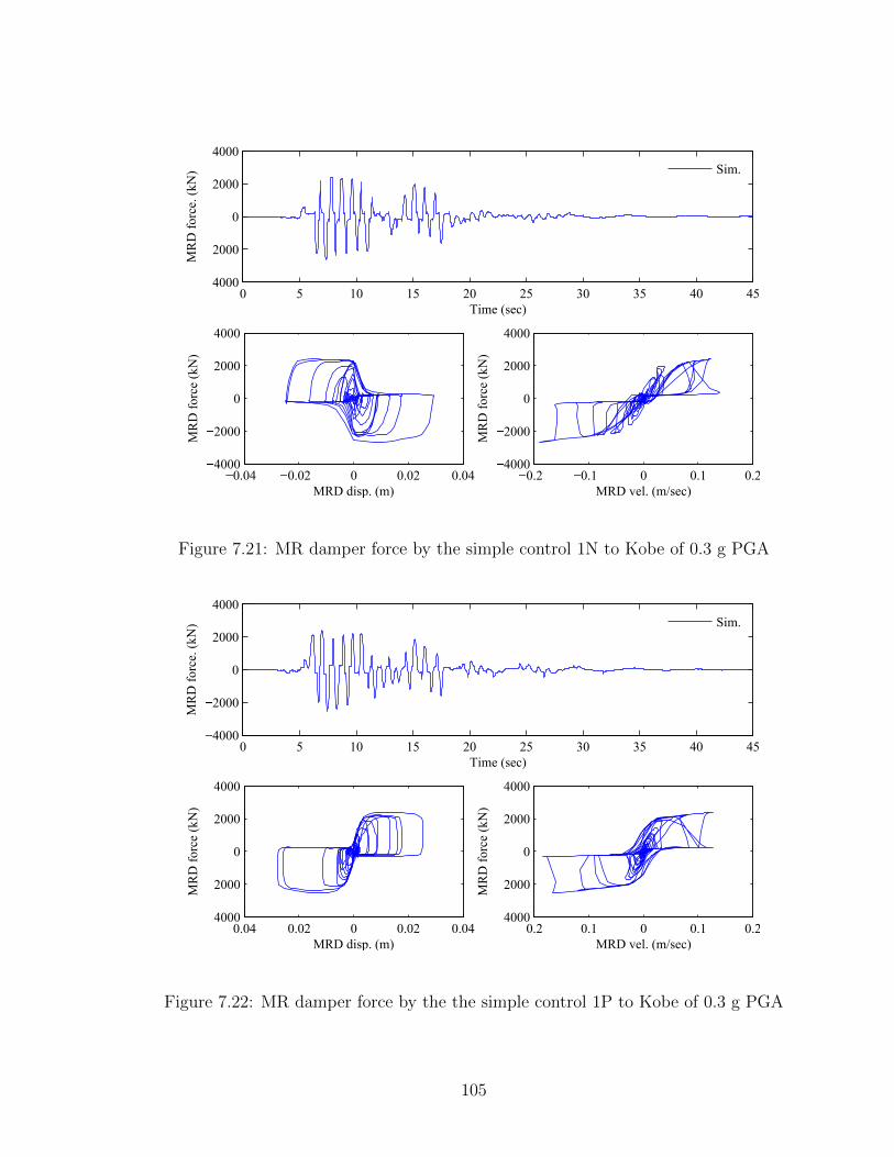
0 5 10 15 20 25 30 35 40 454000
2000
0
2000
4000
Time (sec)
MR
D f
orc
e. (
kN
) Sim.
0.04 0.02 0 0.02 0.044000
2000
0
2000
4000
MRD disp. (m)
MR
D f
orc
e (k
N)
0.2 0.1 0 0.1 0.24000
2000
0
2000
4000
MRD vel. (m/sec)M
RD
forc
e (k
N)
Figure 7.21: MR damper force by the simple control 1N to Kobe of 0.3 g PGA
0 5 10 15 20 25 30 35 40 454000
2000
0
2000
4000
Time (sec)
MR
D f
orc
e. (
kN
) Sim.
0.04 0.02 0 0.02 0.044000
2000
0
2000
4000
MRD disp. (m)
MR
D f
orc
e (k
N)
0.2 0.1 0 0.1 0.24000
2000
0
2000
4000
MRD vel. (m/sec)
MR
D f
orc
e (k
N)
Figure 7.22: MR damper force by the the simple control 1P to Kobe of 0.3 g PGA
105
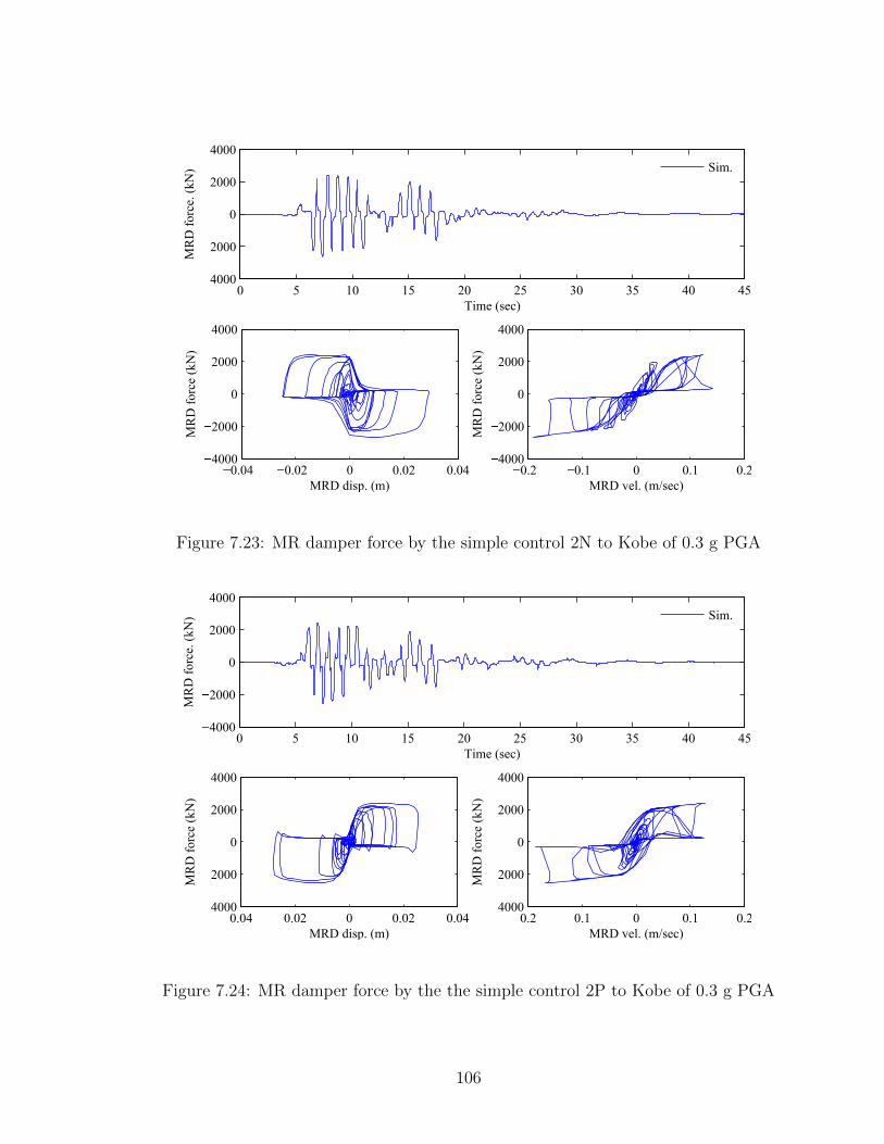
0 5 10 15 20 25 30 35 40 454000
2000
0
2000
4000
Time (sec)
MR
D f
orc
e. (
kN
) Sim.
0.04 0.02 0 0.02 0.044000
2000
0
2000
4000
MRD disp. (m)
MR
D f
orc
e (k
N)
0.2 0.1 0 0.1 0.24000
2000
0
2000
4000
MRD vel. (m/sec)M
RD
forc
e (k
N)
Figure 7.23: MR damper force by the simple control 2N to Kobe of 0.3 g PGA
0 5 10 15 20 25 30 35 40 454000
2000
0
2000
4000
Time (sec)
MR
D f
orc
e. (
kN
) Sim.
0.04 0.02 0 0.02 0.044000
2000
0
2000
4000
MRD disp. (m)
MR
D f
orc
e (k
N)
0.2 0.1 0 0.1 0.24000
2000
0
2000
4000
MRD vel. (m/sec)
MR
D f
orc
e (k
N)
Figure 7.24: MR damper force by the the simple control 2P to Kobe of 0.3 g PGA
106
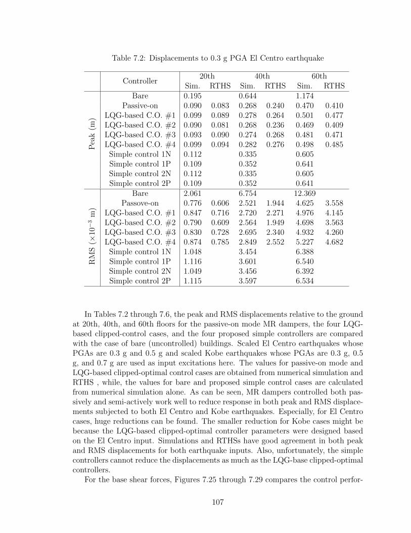
Table 7.2: Displacements to 0.3 g PGA El Centro earthquake
Controller20th 40th 60th
Sim. RTHS Sim. RTHS Sim. RTHSP
eak
(m)
Bare 0.195 0.644 1.174Passive-on 0.090 0.083 0.268 0.240 0.470 0.410
LQG-based C.O. #1 0.099 0.089 0.278 0.264 0.501 0.477LQG-based C.O. #2 0.090 0.081 0.268 0.236 0.469 0.409LQG-based C.O. #3 0.093 0.090 0.274 0.268 0.481 0.471LQG-based C.O. #4 0.099 0.094 0.282 0.276 0.498 0.485
Simple control 1N 0.112 0.335 0.605Simple control 1P 0.109 0.352 0.641Simple control 2N 0.112 0.335 0.605Simple control 2P 0.109 0.352 0.641
RM
S(×
10−3
m)
Bare 2.061 6.754 12.369Passove-on 0.776 0.606 2.521 1.944 4.625 3.558
LQG-based C.O. #1 0.847 0.716 2.720 2.271 4.976 4.145LQG-based C.O. #2 0.790 0.609 2.564 1.949 4.698 3.563LQG-based C.O. #3 0.830 0.728 2.695 2.340 4.932 4.260LQG-based C.O. #4 0.874 0.785 2.849 2.552 5.227 4.682
Simple control 1N 1.048 3.454 6.388Simple control 1P 1.116 3.601 6.540Simple control 2N 1.049 3.456 6.392Simple control 2P 1.115 3.597 6.534
In Tables 7.2 through 7.6, the peak and RMS displacements relative to the groundat 20th, 40th, and 60th floors for the passive-on mode MR dampers, the four LQG-based clipped-control cases, and the four proposed simple controllers are comparedwith the case of bare (uncontrolled) buildings. Scaled El Centro earthquakes whosePGAs are 0.3 g and 0.5 g and scaled Kobe earthquakes whose PGAs are 0.3 g, 0.5g, and 0.7 g are used as input excitations here. The values for passive-on mode andLQG-based clipped-optimal control cases are obtained from numerical simulation andRTHS , while, the values for bare and proposed simple control cases are calculatedfrom numerical simulation alone. As can be seen, MR dampers controlled both pas-sively and semi-actively work well to reduce response in both peak and RMS displace-ments subjected to both El Centro and Kobe earthquakes. Especially, for El Centrocases, huge reductions can be found. The smaller reduction for Kobe cases might bebecause the LQG-based clipped-optimal controller parameters were designed basedon the El Centro input. Simulations and RTHSs have good agreement in both peakand RMS displacements for both earthquake inputs. Also, unfortunately, the simplecontrollers cannot reduce the displacements as much as the LQG-base clipped-optimalcontrollers.
For the base shear forces, Figures 7.25 through 7.29 compares the control perfor-
107
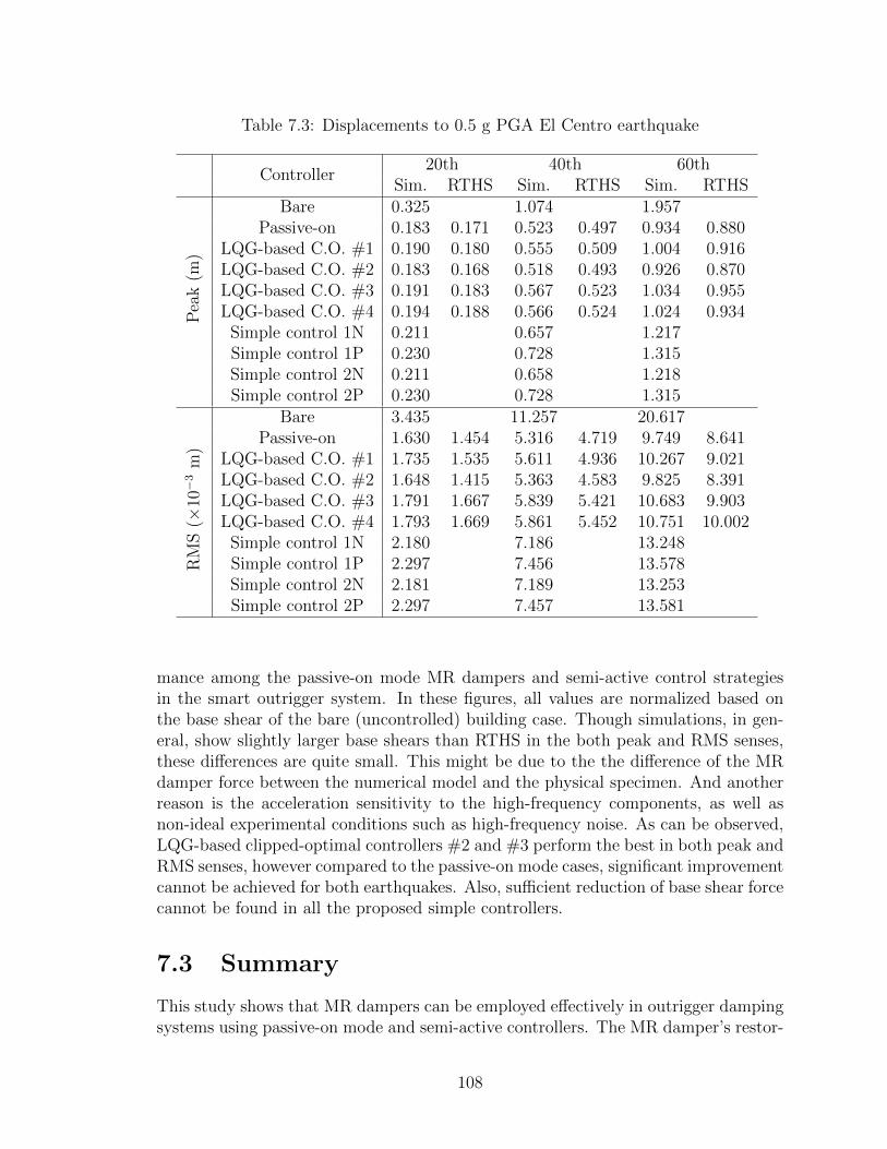
Table 7.3: Displacements to 0.5 g PGA El Centro earthquake
Controller20th 40th 60th
Sim. RTHS Sim. RTHS Sim. RTHSP
eak
(m)
Bare 0.325 1.074 1.957Passive-on 0.183 0.171 0.523 0.497 0.934 0.880
LQG-based C.O. #1 0.190 0.180 0.555 0.509 1.004 0.916LQG-based C.O. #2 0.183 0.168 0.518 0.493 0.926 0.870LQG-based C.O. #3 0.191 0.183 0.567 0.523 1.034 0.955LQG-based C.O. #4 0.194 0.188 0.566 0.524 1.024 0.934
Simple control 1N 0.211 0.657 1.217Simple control 1P 0.230 0.728 1.315Simple control 2N 0.211 0.658 1.218Simple control 2P 0.230 0.728 1.315
RM
S(×
10−3
m)
Bare 3.435 11.257 20.617Passive-on 1.630 1.454 5.316 4.719 9.749 8.641
LQG-based C.O. #1 1.735 1.535 5.611 4.936 10.267 9.021LQG-based C.O. #2 1.648 1.415 5.363 4.583 9.825 8.391LQG-based C.O. #3 1.791 1.667 5.839 5.421 10.683 9.903LQG-based C.O. #4 1.793 1.669 5.861 5.452 10.751 10.002
Simple control 1N 2.180 7.186 13.248Simple control 1P 2.297 7.456 13.578Simple control 2N 2.181 7.189 13.253Simple control 2P 2.297 7.457 13.581
mance among the passive-on mode MR dampers and semi-active control strategiesin the smart outrigger system. In these figures, all values are normalized based onthe base shear of the bare (uncontrolled) building case. Though simulations, in gen-eral, show slightly larger base shears than RTHS in the both peak and RMS senses,these differences are quite small. This might be due to the the difference of the MRdamper force between the numerical model and the physical specimen. And anotherreason is the acceleration sensitivity to the high-frequency components, as well asnon-ideal experimental conditions such as high-frequency noise. As can be observed,LQG-based clipped-optimal controllers #2 and #3 perform the best in both peak andRMS senses, however compared to the passive-on mode cases, significant improvementcannot be achieved for both earthquakes. Also, sufficient reduction of base shear forcecannot be found in all the proposed simple controllers.
7.3 Summary
This study shows that MR dampers can be employed effectively in outrigger dampingsystems using passive-on mode and semi-active controllers. The MR damper’s restor-
108

Table 7.4: Displacements to 0.3 g PGA Kobe earthquake
Controller20th 40th 60th
Sim. RTHS Sim. RTHS Sim. RTHSP
eak
(m)
Bare 0.114 0.160 0.308Passive-on 0.082 0.080 0.131 0.132 0.243 0.243
LQG-based C.O. #1 0.099 0.099 0.140 0.148 0.270 0.273LQG-based C.O. #2 0.082 0.078 0.131 0.128 0.242 0.236LQG-based C.O. #3 0.083 0.079 0.132 0.133 0.245 0.242LQG-based C.O. #4 0.083 0.078 0.131 0.126 0.246 0.236
Simple control 1N 0.090 0.151 0.249Simple control 1P 0.101 0.148 0.287Simple control 2N 0.090 0.151 0.249Simple control 2P 0.101 0.148 0.286
RM
S(×
10−3
m)
Bare 0.429 0.686 1.362Passive-on 0.248 0.237 0.501 0.515 0.975 0.987
LQG-based C.O. #1 0.309 0.304 0.524 0.529 1.038 1.038LQG-based C.O. #2 0.249 0.230 0.499 0.490 0.972 0.944LQG-based C.O. #3 0.251 0.236 0.506 0.514 0.984 0.981LQG-based C.O. #4 0.252 0.234 0.519 0.501 1.008 0.966
Simple control 1N 0.307 0.538 1.076Simple control 1P 0.308 0.597 1.146Simple control 2N 0.307 0.539 1.077Simple control 2P 0.307 0.596 1.144
ing force can be simulated quite well by the proposed MR damper model for the twoearthquake records; however, differences are still present. In particular, discrepanciesbetween simulations and RTHSs were found in the base shear. Moreover, the phys-ical specimen contains no modeling errors, while it is subject to experimental errorsuch as magnitude and time delay. The numerical model provides a good verificationtool for RTHS, however is subject to numerical errors, is only valid within the rangeof behavior for which the model is calibrated, and cannot fully represent the com-plex specimen behavior. Thus, the importance of combining RTHS with numericalsimulation to ensure accurate results is demonstrated.
The effectiveness of semi-active control applied to the outrigger damping systemof a high-rise building is also shown for scaled El Centro and Kobe earthquakes. Inboth simulation and RTHS, LQG-based clipped-optimal controller (e.g., controller#2 which minimizes the translational floor accelerations and #3 which minimizesrotational displacements) provided the best control performance considering bothrelative displacements and base shear. However, the passive-on mode and LQG-based clipped-optimal cases gave similar results, especially in base shear. Also, toimprove the reliability of the smart outrigger damping system for high-rise buildings,different earthquakes should be considered as well as wind excitation.
109
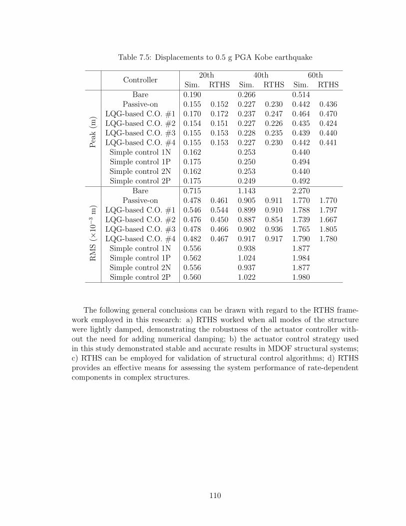
Table 7.5: Displacements to 0.5 g PGA Kobe earthquake
Controller20th 40th 60th
Sim. RTHS Sim. RTHS Sim. RTHSP
eak
(m)
Bare 0.190 0.266 0.514Passive-on 0.155 0.152 0.227 0.230 0.442 0.436
LQG-based C.O. #1 0.170 0.172 0.237 0.247 0.464 0.470LQG-based C.O. #2 0.154 0.151 0.227 0.226 0.435 0.424LQG-based C.O. #3 0.155 0.153 0.228 0.235 0.439 0.440LQG-based C.O. #4 0.155 0.153 0.227 0.230 0.442 0.441
Simple control 1N 0.162 0.253 0.440Simple control 1P 0.175 0.250 0.494Simple control 2N 0.162 0.253 0.440Simple control 2P 0.175 0.249 0.492
RM
S(×
10−3
m)
Bare 0.715 1.143 2.270Passive-on 0.478 0.461 0.905 0.911 1.770 1.770
LQG-based C.O. #1 0.546 0.544 0.899 0.910 1.788 1.797LQG-based C.O. #2 0.476 0.450 0.887 0.854 1.739 1.667LQG-based C.O. #3 0.478 0.466 0.902 0.936 1.765 1.805LQG-based C.O. #4 0.482 0.467 0.917 0.917 1.790 1.780
Simple control 1N 0.556 0.938 1.877Simple control 1P 0.562 1.024 1.984Simple control 2N 0.556 0.937 1.877Simple control 2P 0.560 1.022 1.980
The following general conclusions can be drawn with regard to the RTHS frame-work employed in this research: a) RTHS worked when all modes of the structurewere lightly damped, demonstrating the robustness of the actuator controller with-out the need for adding numerical damping; b) the actuator control strategy usedin this study demonstrated stable and accurate results in MDOF structural systems;c) RTHS can be employed for validation of structural control algorithms; d) RTHSprovides an effective means for assessing the system performance of rate-dependentcomponents in complex structures.
110

Table 7.6: Displacements to 0.7 g PGA Kobe earthquake
Controller20th 40th 60th
Sim. RTHS Sim. RTHS Sim. RTHS
Pea
k(m
)
Bare 0.265 0.373 0.719Passive-on 0.226 0.228 0.325 0.334 0.634 0.645
LQG-based C.O. #1 0.243 0.247 0.335 0.348 0.661 0.671LQG-based C.O. #2 0.225 0.224 0.325 0.326 0.629 0.625LQG-based C.O. #3 0.226 0.229 0.327 0.338 0.634 0.648LQG-based C.O. #4 0.226 0.227 0.326 0.332 0.638 0.646
Simple control 1N 0.234 0.355 0.633Simple control 1P 0.250 0.350 0.699Simple control 2N 0.234 0.355 0.633Simple control 2P 0.250 0.350 0.698
RM
S(×
10−3
m)
Bare 1.001 1.601 3.179Passive-on 0.715 0.711 1.293 1.331 2.541 2.595
LQG-based C.O. #1 0.793 0.792 1.290 1.301 2.570 2.579LQG-based C.O. #2 0.717 0.693 1.286 1.253 2.530 2.459LQG-based C.O. #3 0.715 0.716 1.286 1.350 2.528 2.624LQG-based C.O. #4 0.722 0.712 1.313 1.329 2.575 2.591
Simple control 1N 0.807 1.318 2.648Simple control 1P 0.824 1.470 2.857Simple control 2N 0.808 1.318 2.647Simple control 2P 0.823 1.468 2.853
111

P. on LQG #1 LQG #2 LQG #3 LQG #4 S.C. 1N S.C. 1P S.C. 2N S.C. 2P0
20
40
60
80
100
Rat
io t
o u
nco
ntr
oll
ed (
%)
Peak
P. on LQG #1 LQG #2 LQG #3 LQG #4 S.C. 1N S.C. 1P S.C. 2N S.C. 2P0
20
40
60
80
100
Rat
io t
o u
nco
ntr
oll
ed (
%)
RMS
Sim. RTHS
Figure 7.25: Base shear to 0.3 g PGA El Centro earthquake
P. on LQG #1 LQG #2 LQG #3 LQG #4 S.C. 1N S.C. 1P S.C. 2N S.C. 2P0
20
40
60
80
100
Rat
io t
o u
nco
ntr
oll
ed (
%)
Peak
P. on LQG #1 LQG #2 LQG #3 LQG #4 S.C. 1N S.C. 1P S.C. 2N S.C. 2P0
20
40
60
80
100
Rat
io t
o u
nco
ntr
oll
ed (
%)
RMS
Sim. RTHS
Figure 7.26: Base shear to 0.5 g PGA El Centro earthquake
112

P. on LQG #1 LQG #2 LQG #3 LQG #4 S.C. 1N S.C. 1P S.C. 2N S.C. 2P0
20
40
60
80
100
Rat
io t
o u
nco
ntr
oll
ed (
%)
Peak
P. on LQG #1 LQG #2 LQG #3 LQG #4 S.C. 1N S.C. 1P S.C. 2N S.C. 2P0
20
40
60
80
100
Rat
io t
o u
nco
ntr
oll
ed (
%)
RMS
Sim. RTHS
Figure 7.27: Base shear to 0.3 g PGA Kobe earthquake
P. on LQG #1 LQG #2 LQG #3 LQG #4 S.C. 1N S.C. 1P S.C. 2N S.C. 2P0
20
40
60
80
100
Rat
io t
o u
nco
ntr
oll
ed (
%)
Peak
P. on LQG #1 LQG #2 LQG #3 LQG #4 S.C. 1N S.C. 1P S.C. 2N S.C. 2P0
20
40
60
80
100
Rat
io t
o u
nco
ntr
oll
ed (
%)
RMS
Sim. RTHS
Figure 7.28: Base shear to 0.5 g PGA Kobe earthquake
113

P. on LQG #1 LQG #2 LQG #3 LQG #4 S.C. 1N S.C. 1P S.C. 2N S.C. 2P0
20
40
60
80
100
Rat
io t
o u
nco
ntr
oll
ed (
%)
Peak
P. on LQG #1 LQG #2 LQG #3 LQG #4 S.C. 1N S.C. 1P S.C. 2N S.C. 2P0
20
40
60
80
100
Rat
io t
o u
nco
ntr
oll
ed (
%)
RMS
Sim. RTHS
Figure 7.29: Base shear to 0.7 g PGA Kobe earthquake
114
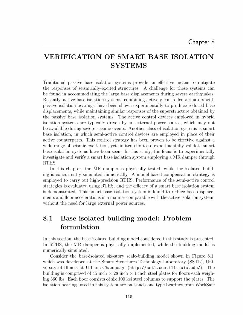
Chapter 8
VERIFICATION OF SMART BASE ISOLATION
SYSTEMS
Traditional passive base isolation systems provide an effective means to mitigatethe responses of seismically-excited structures. A challenge for these systems canbe found in accommodating the large base displacements during severe earthquakes.Recently, active base isolation systems, combining actively controlled actuators withpassive isolation bearings, have been shown experimentally to produce reduced basedisplacements, while maintaining similar responses of the superstructure obtained bythe passive base isolation systems. The active control devices employed in hybridisolation systems are typically driven by an external power source, which may notbe available during severe seismic events. Another class of isolation systems is smartbase isolation, in which semi-active control devices are employed in place of theiractive counterparts. This control strategy has been proven to be effective against awide range of seismic excitation, yet limited efforts to experimentally validate smartbase isolation systems have been seen. In this study, the focus is to experimentallyinvestigate and verify a smart base isolation system employing a MR damper throughRTHS.
In this chapter, the MR damper is physically tested, while the isolated build-ing is concurrently simulated numerically. A model-based compensation strategy isemployed to carry out high-precision RTHS. Performance of the semi-active controlstrategies is evaluated using RTHS, and the efficacy of a smart base isolation systemis demonstrated. This smart base isolation system is found to reduce base displace-ments and floor accelerations in a manner comparable with the active isolation system,without the need for large external power sources.
8.1 Base-isolated building model: Problem
formulation
In this section, the base-isolated building model considered in this study is presented.In RTHS, the MR damper is physically implemented, while the building model isnumerically simulated.
Consider the base-isolated six-story scale-building model shown in Figure 8.1,which was developed at the Smart Structures Technology Laboratory (SSTL), Uni-versity of Illinois at Urbana-Champaign (http://sstl.cee.illinois.edu/). Thebuilding is comprised of 45 inch × 28 inch × 1 inch steel plates for floors each weigh-ing 360 lbs. Each floor consists of six 100 ksi steel columns to support the plates. Theisolation bearings used in this system are ball-and-cone type bearings from WorkSafe
115
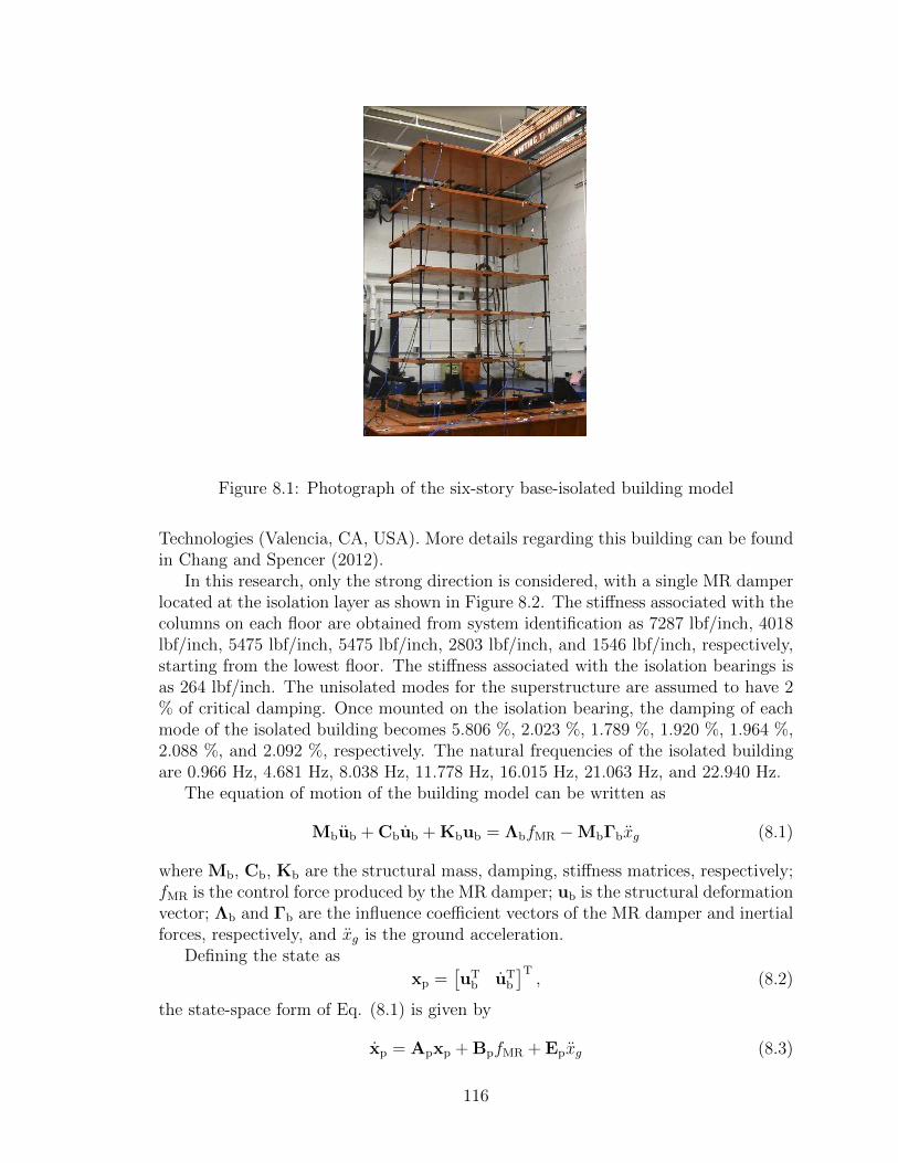
Figure 8.1: Photograph of the six-story base-isolated building model
Technologies (Valencia, CA, USA). More details regarding this building can be foundin Chang and Spencer (2012).
In this research, only the strong direction is considered, with a single MR damperlocated at the isolation layer as shown in Figure 8.2. The stiffness associated with thecolumns on each floor are obtained from system identification as 7287 lbf/inch, 4018lbf/inch, 5475 lbf/inch, 5475 lbf/inch, 2803 lbf/inch, and 1546 lbf/inch, respectively,starting from the lowest floor. The stiffness associated with the isolation bearings isas 264 lbf/inch. The unisolated modes for the superstructure are assumed to have 2% of critical damping. Once mounted on the isolation bearing, the damping of eachmode of the isolated building becomes 5.806 %, 2.023 %, 1.789 %, 1.920 %, 1.964 %,2.088 %, and 2.092 %, respectively. The natural frequencies of the isolated buildingare 0.966 Hz, 4.681 Hz, 8.038 Hz, 11.778 Hz, 16.015 Hz, 21.063 Hz, and 22.940 Hz.
The equation of motion of the building model can be written as
Mbub + Cbub + Kbub = ΛbfMR −MbΓbxg (8.1)
where Mb, Cb, Kb are the structural mass, damping, stiffness matrices, respectively;fMR is the control force produced by the MR damper; ub is the structural deformationvector; Λb and Γb are the influence coefficient vectors of the MR damper and inertialforces, respectively, and xg is the ground acceleration.
Defining the state as
xp =[uTb uT
b
]T, (8.2)
the state-space form of Eq. (8.1) is given by
xp = Apxp + BpfMR + Epxg (8.3)
116

MR damper
Six-stroy building
Bearing
Figure 8.2: Schematic illustration of analysis model
yp = Cypxp + DypfMR + Fypxg + vp (8.4)
zp = Czpxp + DzpfMR + Fzpxg (8.5)
where yp presents the measured structural responses; vp is the measurement noise;zp corresponds to the regulated structural responses. Ap, Bp, Cyp, Czp, Dyp, Dzp,Ep, Fyp, and Fzp are appropriately chosen matrices corresponding to the associatedstate-space equations.
8.2 Results
In this section, the hysteresis force-displacement loops and seismic performance ob-tained from numerical studies and RTHS are shown. For the RTHS, the small-scaleMR damper shown in Figure 4.1 is used, and for the numerical simulation, the MRdamper model created in Section 4.1 is used. To adjust the capacity of the MRdamper to the target building, the displacement of the MR damper is scaled suchthat 1 inch in the physical MR damper corresponds to 10 inches in the numericalmodel of the smart base-isolated building. The output force of the MR damper is notscaled (i.e., 1 lbf in the physical system is 1 lbf in the numerical model).
8.2.1 Numerical simulation
The results obtained from numerical simulation are shown here. The earthquakes usedin this study are El Centro (1994, Northridge Earthquake, El Centro record, fault-parallel), Ji-ji (1999, station TCU 068, North-South component), Kobe (1995, JMAstation, East-West component), Newhall (1994, Northridge Earthquake, Newhall
117

county, fault-parallel), and Sylmar (1994, Northridge Earthquake, Sylmar station,fault-parallel) (Narasimhan et al., 2008). The PGAs of these earthquakes are scaledto 0.2 g and 0.5 g.
To compare the performance of a variety of semi-active controllers, three LQG-based clipped-optimal controllers are designed and the simple algorithms proposedin Section 6.4 are applied as well. The three LQG-based clipped-optimal controllersincluding acceleration weighting, inter-story drift weighting, and relative displacementweighting are designed. For the Kalman filter in Eqs. (7.10) and (7.11), this studyassumes that the absolute floor accelerations at the base and 1st through 6th floorsare available to estimate the required force. In addition to these two semi-activecontrollers, three passive systems are also considered: (i) an uncontrolled passivebase-isolated building, (ii) a base-isolated building with an MR damper in passive-offmode (i.e., the input current is 0), and (iii) a base-isolated building with an MRdamper in passive-on mode (i.e., the input current is 2.0 A). For the uncontrolledpassive base isolation case, simulation studies are carried out.
Figures 8.3 to 8.9 show the hystetetic force-displacement loops obtained fromthe semi-active controllers to 0.2 g PGA earthquakes. As expected, pseudo-negativestiffness can be found by the LQG-based clipped-optimal control with accelerationweighting, the LQG-based clipped-optimal control with inter-story drift weighting,the simple control 1N, and the simple control 2N while, the LQG-based clipped-optimal control with relative displacement weighting, the simple control 1P, and thesimple control 2P produced positive stiffness. The hysteresis loops subjected to 0.5g PGA earthquakes are depicted in Figures 8.10 to 8.16. As can be seen in Figures8.10 and 8.11, clear pseudo-negative stiffness cannot be found in the hysteresis loopsproduced by the LQG-based clipped optimal controllers with acceleration weightingand inter-story drift weighting, while the other controllers still show the expectedproperties.
The responses of the base displacement and the absolute accelerations of the basethrough 6th floor are summarized in Tables 8.1 through 8.5. Figures 8.17 through8.28 compare the ratios of the peak and RMS responses based on the uncontrolledcase (i.e., the passive base isolation). As can be seen, generally, the controllers pro-ducing pseudo-negative stiffness shows better performance than the positive stiffnesscontrollers. However, the proposed simple algorithms cannot show comparable per-formance with the LQG-based clipped optimal controllers, especially in the responseaccelerations of the upper floor. These results show that it is difficult for the proposedsimple algorithms to control complicated structures.
118
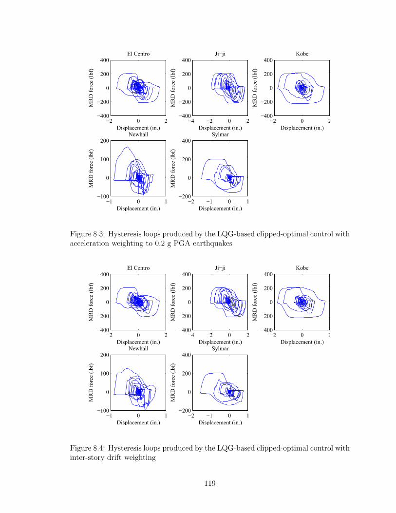
−2 0 2−400
−200
0
200
400
Displacement (in.)
MR
D f
orc
e (l
bf)
El Centro
−4 −2 0 2−400
−200
0
200
400
Displacement (in.)
MR
D f
orc
e (l
bf)
Ji−ji
−2 0 2−400
−200
0
200
400
Displacement (in.)
MR
D f
orc
e (l
bf)
Kobe
−1 0 1−100
0
100
200
Displacement (in.)
MR
D f
orc
e (l
bf)
Newhall
−2 −1 0 1−200
0
200
400
Displacement (in.)
MR
D f
orc
e (l
bf)
Sylmar
Figure 8.3: Hysteresis loops produced by the LQG-based clipped-optimal control withacceleration weighting to 0.2 g PGA earthquakes
−2 0 2−400
−200
0
200
400
Displacement (in.)
MR
D f
orc
e (l
bf)
El Centro
−4 −2 0 2−400
−200
0
200
400
Displacement (in.)
MR
D f
orc
e (l
bf)
Ji−ji
−2 0 2−400
−200
0
200
400
Displacement (in.)
MR
D f
orc
e (l
bf)
Kobe
−1 0 1−100
0
100
200
Displacement (in.)
MR
D f
orc
e (l
bf)
Newhall
−2 −1 0 1−200
0
200
400
Displacement (in.)
MR
D f
orc
e (l
bf)
Sylmar
Figure 8.4: Hysteresis loops produced by the LQG-based clipped-optimal control withinter-story drift weighting
119

−2 0 2−400
−200
0
200
400
Displacement (in.)
MR
D f
orc
e (l
bf)
El Centro
−2 0 2−400
−200
0
200
400
Displacement (in.)
MR
D f
orc
e (l
bf)
Ji−ji
−4 −2 0 2−400
−200
0
200
400
Displacement (in.)
MR
D f
orc
e (l
bf)
Kobe
−1 −0.5 0 0.5−200
−100
0
100
200
Displacement (in.)
MR
D f
orc
e (l
bf)
Newhall
−2 −1 0 1−400
−200
0
200
Displacement (in.)
MR
D f
orc
e (l
bf)
Sylmar
Figure 8.5: Hysteresis loops produced by the LQG-based clipped-optimal control withrelative displacement weighting to 0.2 g PGA earthquakes
−2 0 2−400
−200
0
200
400
Displacement (in.)
MR
D f
orc
e (l
bf)
El Centro
−5 0 5−400
−200
0
200
400
Displacement (in.)
MR
D f
orc
e (l
bf)
Ji−ji
−4 −2 0 2−400
−200
0
200
400
Displacement (in.)
MR
D f
orc
e (l
bf)
Kobe
−1 −0.5 0 0.5−200
−100
0
100
200
Displacement (in.)
MR
D f
orc
e (l
bf)
Newhall
−2 −1 0 1−400
−200
0
200
400
Displacement (in.)
MR
D f
orc
e (l
bf)
Sylmar
Figure 8.6: Hysteresis loops produced by the simple control 1N by Eq. (6.18) to 0.2g PGA earthquakes
120
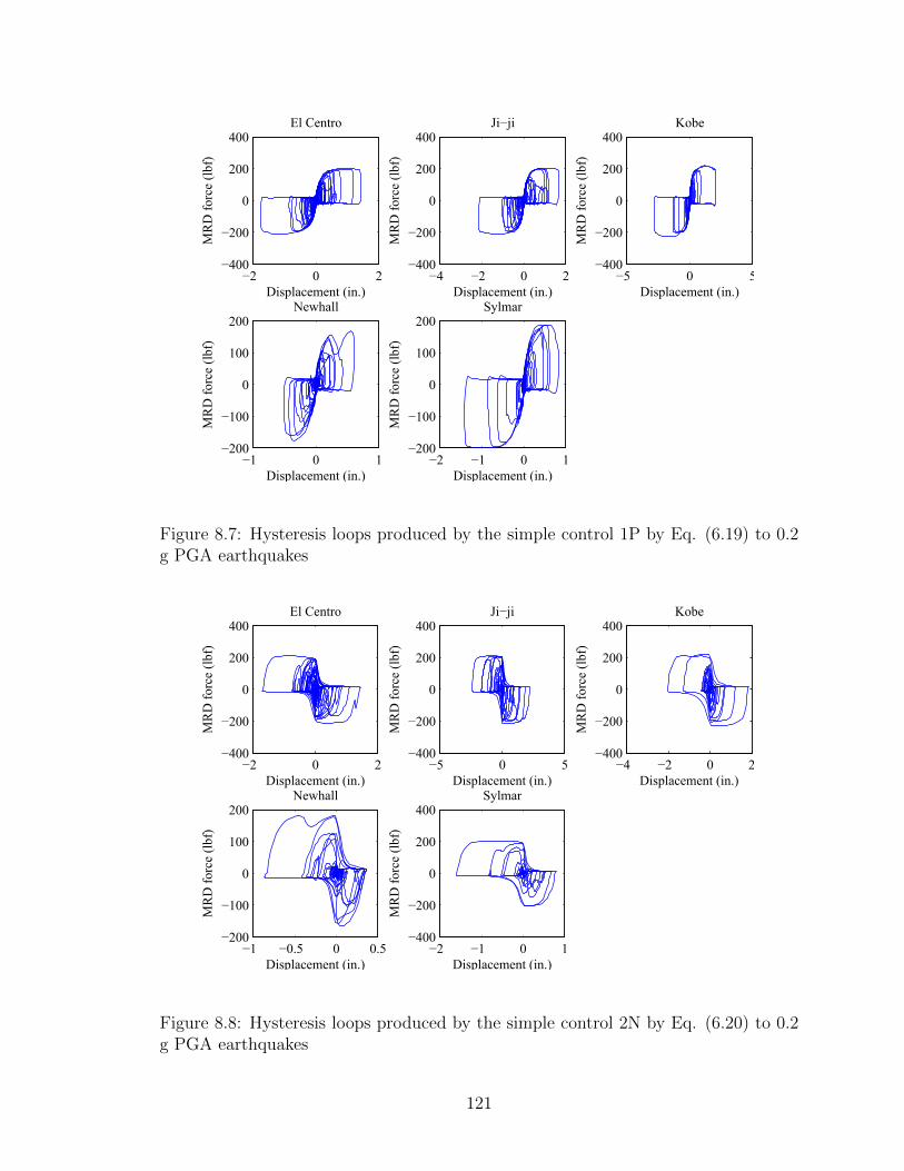
−2 0 2−400
−200
0
200
400
Displacement (in.)
MR
D f
orc
e (l
bf)
El Centro
−4 −2 0 2−400
−200
0
200
400
Displacement (in.)
MR
D f
orc
e (l
bf)
Ji−ji
−5 0 5−400
−200
0
200
400
Displacement (in.)
MR
D f
orc
e (l
bf)
Kobe
−1 0 1−200
−100
0
100
200
Displacement (in.)
MR
D f
orc
e (l
bf)
Newhall
−2 −1 0 1−200
−100
0
100
200
Displacement (in.)
MR
D f
orc
e (l
bf)
Sylmar
Figure 8.7: Hysteresis loops produced by the simple control 1P by Eq. (6.19) to 0.2g PGA earthquakes
−2 0 2−400
−200
0
200
400
Displacement (in.)
MR
D f
orc
e (l
bf)
El Centro
−5 0 5−400
−200
0
200
400
Displacement (in.)
MR
D f
orc
e (l
bf)
Ji−ji
−4 −2 0 2−400
−200
0
200
400
Displacement (in.)
MR
D f
orc
e (l
bf)
Kobe
−1 −0.5 0 0.5−200
−100
0
100
200
Displacement (in.)
MR
D f
orc
e (l
bf)
Newhall
−2 −1 0 1−400
−200
0
200
400
Displacement (in.)
MR
D f
orc
e (l
bf)
Sylmar
Figure 8.8: Hysteresis loops produced by the simple control 2N by Eq. (6.20) to 0.2g PGA earthquakes
121

−2 0 2−400
−200
0
200
400
Displacement (in.)
MR
D f
orc
e (l
bf)
El Centro
−4 −2 0 2−400
−200
0
200
400
Displacement (in.)
MR
D f
orc
e (l
bf)
Ji−ji
−5 0 5−400
−200
0
200
400
Displacement (in.)
MR
D f
orc
e (l
bf)
Kobe
−1 0 1−200
−100
0
100
200
Displacement (in.)
MR
D f
orc
e (l
bf)
Newhall
−2 −1 0 1−200
−100
0
100
200
Displacement (in.)
MR
D f
orc
e (l
bf)
Sylmar
Figure 8.9: Hysteresis loops produced by the simple control 2P by Eq. (6.21) to 0.2g PGA earthquakes
−5 0 5−400
−200
0
200
400
Displacement (in.)
MR
D f
orc
e (l
bf)
El Centro
−10 0 10−400
−200
0
200
400
Displacement (in.)
MR
D f
orc
e (l
bf)
Ji−ji
−10 0 10−400
−200
0
200
400
Displacement (in.)
MR
D f
orc
e (l
bf)
Kobe
−4 −2 0 2−400
−200
0
200
400
Displacement (in.)
MR
D f
orc
e (l
bf)
Newhall
−5 0 5−400
−200
0
200
400
Displacement (in.)
MR
D f
orc
e (l
bf)
Sylmar
Figure 8.10: Hysteresis loops produced by the LQG-based clipped-optimal controlwith acceleration weighting to 0.5 g PGA earthquakes
122

−5 0 5−400
−200
0
200
400
Displacement (in.)
MR
D f
orc
e (l
bf)
El Centro
−10 0 10−400
−200
0
200
400
Displacement (in.)
MR
D f
orc
e (l
bf)
Ji−ji
−10 0 10−400
−200
0
200
400
Displacement (in.)
MR
D f
orc
e (l
bf)
Kobe
−4 −2 0 2−400
−200
0
200
400
Displacement (in.)
MR
D f
orc
e (l
bf)
Newhall
−5 0 5−400
−200
0
200
400
Displacement (in.)
MR
D f
orc
e (l
bf)
Sylmar
Figure 8.11: Hysteresis loops produced by the LQG-based clipped-optimal controlwith inter-story drift weighting
−10 −5 0 5−400
−200
0
200
400
Displacement (in.)
MR
D f
orc
e (l
bf)
El Centro
−10 −5 0 5−400
−200
0
200
400
Displacement (in.)
MR
D f
orc
e (l
bf)
Ji−ji
−10 0 10−400
−200
0
200
400
Displacement (in.)
MR
D f
orc
e (l
bf)
Kobe
−2 0 2−400
−200
0
200
400
Displacement (in.)
MR
D f
orc
e (l
bf)
Newhall
−5 0 5−400
−200
0
200
400
Displacement (in.)
MR
D f
orc
e (l
bf)
Sylmar
Figure 8.12: Hysteresis loops produced by the LQG-based clipped-optimal controlwith relative displacement weighting to 0.5 g PGA earthquakes
123

−10 −5 0 5−400
−200
0
200
400
Displacement (in.)
MR
D f
orc
e (l
bf)
El Centro
−10 0 10−400
−200
0
200
400
Displacement (in.)
MR
D f
orc
e (l
bf)
Ji−ji
−10 0 10−400
−200
0
200
400
Displacement (in.)
MR
D f
orc
e (l
bf)
Kobe
−4 −2 0 2−400
−200
0
200
400
Displacement (in.)
MR
D f
orc
e (l
bf)
Newhall
−5 0 5−400
−200
0
200
400
Displacement (in.)
MR
D f
orc
e (l
bf)
Sylmar
Figure 8.13: Hysteresis loops produced by the simple control 1N by Eq. (6.18) to 0.5g PGA earthquakes
−10 −5 0 5−400
−200
0
200
400
Displacement (in.)
MR
D f
orc
e (l
bf)
El Centro
−10 0 10−400
−200
0
200
400
Displacement (in.)
MR
D f
orc
e (l
bf)
Ji−ji
−10 0 10−400
−200
0
200
400
Displacement (in.)
MR
D f
orc
e (l
bf)
Kobe
−2 0 2 4−400
−200
0
200
400
Displacement (in.)
MR
D f
orc
e (l
bf)
Newhall
−5 0 5−400
−200
0
200
400
Displacement (in.)
MR
D f
orc
e (l
bf)
Sylmar
Figure 8.14: Hysteresis loops produced by the simple control 1P by Eq. (6.19) to 0.5g PGA earthquakes
124
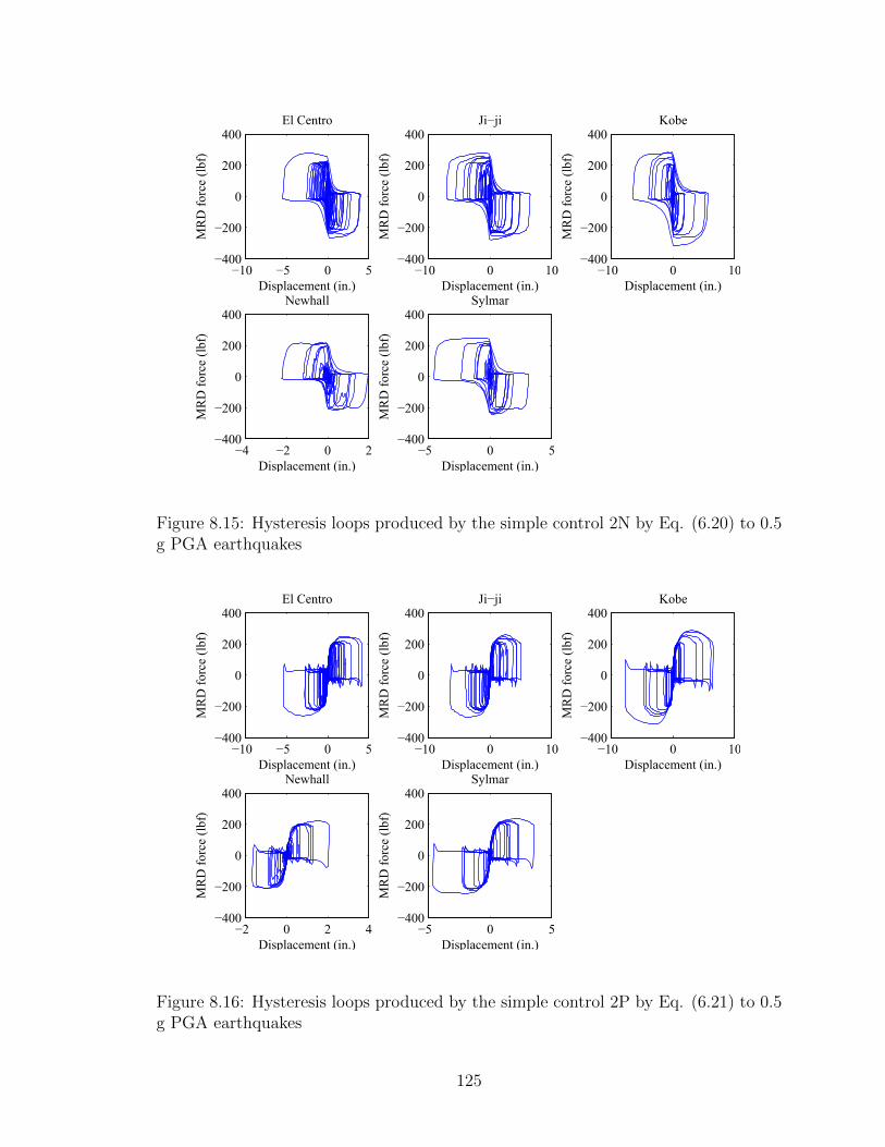
−10 −5 0 5−400
−200
0
200
400
Displacement (in.)
MR
D f
orc
e (l
bf)
El Centro
−10 0 10−400
−200
0
200
400
Displacement (in.)
MR
D f
orc
e (l
bf)
Ji−ji
−10 0 10−400
−200
0
200
400
Displacement (in.)
MR
D f
orc
e (l
bf)
Kobe
−4 −2 0 2−400
−200
0
200
400
Displacement (in.)
MR
D f
orc
e (l
bf)
Newhall
−5 0 5−400
−200
0
200
400
Displacement (in.)
MR
D f
orc
e (l
bf)
Sylmar
Figure 8.15: Hysteresis loops produced by the simple control 2N by Eq. (6.20) to 0.5g PGA earthquakes
−10 −5 0 5−400
−200
0
200
400
Displacement (in.)
MR
D f
orc
e (l
bf)
El Centro
−10 0 10−400
−200
0
200
400
Displacement (in.)
MR
D f
orc
e (l
bf)
Ji−ji
−10 0 10−400
−200
0
200
400
Displacement (in.)
MR
D f
orc
e (l
bf)
Kobe
−2 0 2 4−400
−200
0
200
400
Displacement (in.)
MR
D f
orc
e (l
bf)
Newhall
−5 0 5−400
−200
0
200
400
Displacement (in.)
MR
D f
orc
e (l
bf)
Sylmar
Figure 8.16: Hysteresis loops produced by the simple control 2P by Eq. (6.21) to 0.5g PGA earthquakes
125

Table 8.1: Peak and RMS values to the scaled El Centro earthquakes
ControllerDisp. (in.) Acceleration (g)
Base Base 1 2 3 4 5 6
0.2
gP
GA
Pea
kUncontrolled 2.616 0.293 0.298 0.298 0.291 0.282 0.292 0.337Passive-off 2.395 0.279 0.279 0.280 0.275 0.268 0.274 0.305Passive-on 1.218 0.266 0.274 0.272 0.233 0.219 0.256 0.395LQG w/ A. 1.592 0.234 0.237 0.221 0.197 0.207 0.224 0.286
LQG w/ I.D. 1.632 0.216 0.217 0.211 0.187 0.207 0.231 0.260LQG w/ R.D. 1.570 0.321 0.355 0.350 0.379 0.338 0.415 0.558
Simple control 1N 1.676 0.353 0.344 0.304 0.310 0.349 0.343 0.440Simple control 1P 1.758 0.417 0.347 0.483 0.468 0.400 0.457 0.555Simple control 2N 1.701 0.318 0.331 0.311 0.292 0.357 0.370 0.437Simple control 2P 1.742 0.427 0.378 0.478 0.474 0.384 0.468 0.570
RM
S
Uncontrolled 0.673 0.067 0.068 0.070 0.072 0.073 0.076 0.080Passive-off 0.561 0.058 0.059 0.060 0.062 0.063 0.065 0.070Passive-on 0.227 0.044 0.045 0.045 0.046 0.047 0.054 0.070LQG w/ A. 0.358 0.042 0.042 0.042 0.043 0.045 0.049 0.057
LQG w/ I.D. 0.369 0.042 0.042 0.043 0.044 0.045 0.048 0.055LQG w/ R.D. 0.286 0.066 0.064 0.062 0.064 0.067 0.073 0.091
Simple control 1N 0.340 0.079 0.074 0.070 0.068 0.073 0.081 0.102Simple control 1P 0.322 0.075 0.072 0.071 0.070 0.075 0.083 0.103Simple control 2N 0.343 0.075 0.069 0.062 0.062 0.067 0.075 0.101Simple control 2P 0.320 0.074 0.072 0.069 0.070 0.073 0.081 0.103
0.5
gP
GA
Pea
k
Uncontrolled 6.539 0.732 0.745 0.744 0.728 0.705 0.729 0.843Passive-off 6.172 0.713 0.706 0.694 0.688 0.677 0.712 0.768Passive-on 4.671 0.771 0.771 0.741 0.701 0.694 0.829 0.930LQG w/ A. 4.906 0.679 0.697 0.675 0.609 0.676 0.679 0.756
LQG w/ I.D. 4.863 0.650 0.687 0.674 0.577 0.651 0.666 0.727LQG w/ R.D. 5.323 0.904 0.941 0.861 0.855 0.829 0.910 1.049
Simple control 1N 5.457 0.847 0.856 0.798 0.677 0.738 0.866 1.164Simple control 1P 5.415 0.851 0.865 0.879 0.941 0.883 0.911 1.046Simple control 2N 5.482 0.836 0.841 0.784 0.712 0.731 0.877 1.151Simple control 2P 5.391 0.876 0.848 0.902 0.938 0.898 0.980 1.099
RM
S
Uncontrolled 1.682 0.166 0.170 0.176 0.179 0.183 0.189 0.201Passive-off 1.518 0.152 0.155 0.160 0.164 0.167 0.173 0.182Passive-on 0.858 0.129 0.128 0.123 0.123 0.126 0.139 0.185LQG w/ A. 0.995 0.112 0.112 0.112 0.115 0.119 0.125 0.143
LQG w/ I.D. 1.006 0.110 0.111 0.112 0.115 0.119 0.125 0.139LQG w/ R.D. 1.026 0.163 0.161 0.156 0.160 0.164 0.179 0.217
Simple control 1N 1.134 0.156 0.151 0.141 0.144 0.152 0.158 0.203Simple control 1P 1.077 0.172 0.167 0.164 0.166 0.172 0.188 0.227Simple control 2N 1.138 0.153 0.147 0.138 0.141 0.148 0.156 0.199Simple control 2P 1.073 0.174 0.168 0.166 0.167 0.174 0.191 0.230
126

Table 8.2: Peak and RMS values to the scaled Ji-ji earthquakes
ControllerDisp. (in.) Acceleration (g)
Base Base 1 2 3 4 5 6
0.2
gP
GA
Pea
kUncontrolled 2.909 0.295 0.300 0.306 0.311 0.316 0.333 0.352Passive-off 2.848 0.301 0.305 0.298 0.317 0.332 0.344 0.374Passive-on 1.445 0.271 0.237 0.269 0.289 0.278 0.311 0.342LQG w/ A. 2.021 0.292 0.304 0.294 0.244 0.261 0.291 0.353
LQG w/ I.D. 2.103 0.293 0.309 0.283 0.259 0.272 0.302 0.333LQG w/ R.D. 1.935 0.376 0.341 0.439 0.353 0.393 0.376 0.435
Simple control 1N 2.427 0.414 0.406 0.423 0.413 0.397 0.449 0.486Simple control 1P 2.152 0.400 0.412 0.428 0.429 0.414 0.420 0.537Simple control 2N 2.451 0.430 0.406 0.414 0.383 0.393 0.404 0.474Simple control 2P 2.142 0.369 0.367 0.444 0.417 0.423 0.416 0.551
RM
S
Uncontrolled 1.016 0.099 0.102 0.106 0.108 0.110 0.112 0.114Passive-off 0.855 0.086 0.088 0.090 0.092 0.094 0.096 0.100Passive-on 0.393 0.052 0.053 0.054 0.055 0.057 0.058 0.062LQG w/ A. 0.585 0.060 0.060 0.060 0.062 0.063 0.066 0.072
LQG w/ I.D. 0.602 0.061 0.061 0.062 0.063 0.064 0.066 0.072LQG w/ R.D. 0.431 0.068 0.068 0.070 0.069 0.072 0.074 0.083
Simple control 1N 0.617 0.074 0.072 0.073 0.073 0.077 0.081 0.088Simple control 1P 0.460 0.074 0.074 0.074 0.076 0.077 0.080 0.091Simple control 2N 0.618 0.072 0.070 0.070 0.071 0.075 0.077 0.087Simple control 2P 0.459 0.073 0.073 0.073 0.074 0.076 0.079 0.091
0.5
gP
GA
Pea
k
Uncontrolled 7.272 0.738 0.750 0.765 0.777 0.791 0.832 0.880Passive-off 7.182 0.714 0.743 0.736 0.772 0.814 0.838 0.931Passive-on 6.135 0.886 0.900 0.829 0.841 0.970 0.929 1.051LQG w/ A. 6.144 0.838 0.836 0.830 0.758 0.739 0.780 0.972
LQG w/ I.D. 6.150 0.800 0.812 0.815 0.771 0.742 0.774 0.942LQG w/ R.D. 6.160 0.843 0.863 0.907 0.954 0.913 0.958 1.159
Simple control 1N 7.083 1.010 0.843 0.976 0.906 0.976 0.979 0.938Simple control 1P 6.432 0.911 0.860 0.916 0.965 0.974 0.866 1.006Simple control 2N 7.103 0.931 0.849 0.984 0.908 0.970 0.972 1.011Simple control 2P 6.426 0.922 0.868 0.919 0.981 1.022 0.917 1.063
RM
S
Uncontrolled 2.540 0.249 0.255 0.264 0.270 0.274 0.280 0.286Passive-off 2.296 0.227 0.232 0.240 0.245 0.249 0.255 0.261Passive-on 1.362 0.159 0.160 0.160 0.164 0.167 0.172 0.188LQG w/ A. 1.571 0.163 0.164 0.166 0.170 0.172 0.177 0.189
LQG w/ I.D. 1.580 0.163 0.164 0.167 0.170 0.172 0.177 0.188LQG w/ R.D. 1.446 0.192 0.190 0.191 0.194 0.197 0.211 0.232
Simple control 1N 1.810 0.192 0.190 0.192 0.195 0.202 0.206 0.222Simple control 1P 1.517 0.197 0.196 0.199 0.203 0.205 0.221 0.235Simple control 2N 1.812 0.190 0.189 0.192 0.193 0.201 0.204 0.222Simple control 2P 1.514 0.199 0.196 0.199 0.204 0.206 0.225 0.238
127

Table 8.3: Peak and RMS values to the scaled Kobe earthquakes
ControllerDisp. (in.) Acceleration (g)
Base Base 1 2 3 4 5 6
0.2
gP
GA
Pea
kUncontrolled 3.275 0.320 0.331 0.344 0.351 0.355 0.361 0.372Passive-off 3.178 0.337 0.342 0.352 0.353 0.364 0.355 0.375Passive-on 1.875 0.291 0.283 0.255 0.283 0.321 0.381 0.397LQG w/ A. 1.778 0.215 0.245 0.269 0.247 0.236 0.264 0.303
LQG w/ I.D. 1.802 0.253 0.257 0.262 0.249 0.281 0.260 0.287LQG w/ R.D. 2.615 0.366 0.442 0.434 0.407 0.395 0.529 0.546
Simple control 1N 2.033 0.433 0.495 0.300 0.473 0.475 0.365 0.563Simple control 1P 2.814 0.489 0.463 0.482 0.501 0.617 0.514 0.678Simple control 2N 2.053 0.412 0.445 0.267 0.427 0.487 0.367 0.566Simple control 2P 2.793 0.518 0.434 0.516 0.553 0.612 0.510 0.685
RM
S
Uncontrolled 0.918 0.088 0.091 0.095 0.098 0.100 0.103 0.106Passive-off 0.731 0.071 0.073 0.077 0.079 0.081 0.083 0.086Passive-on 0.248 0.036 0.037 0.039 0.042 0.044 0.047 0.054LQG w/ A. 0.298 0.034 0.034 0.036 0.037 0.039 0.041 0.046
LQG w/ I.D. 0.310 0.035 0.036 0.037 0.038 0.040 0.042 0.046LQG w/ R.D. 0.363 0.059 0.060 0.062 0.063 0.066 0.069 0.079
Simple control 1N 0.322 0.062 0.059 0.052 0.060 0.062 0.063 0.075Simple control 1P 0.415 0.071 0.069 0.070 0.073 0.078 0.080 0.092Simple control 2N 0.325 0.059 0.055 0.048 0.055 0.059 0.062 0.075Simple control 2P 0.411 0.070 0.068 0.068 0.073 0.076 0.079 0.092
0.5
gP
GA
Pea
k
Uncontrolled 8.187 0.799 0.826 0.861 0.878 0.889 0.902 0.929Passive-off 7.994 0.806 0.837 0.869 0.879 0.885 0.878 0.895Passive-on 6.407 0.860 0.817 0.810 0.879 1.007 1.031 1.104LQG w/ A. 6.009 0.741 0.866 0.765 0.820 0.842 0.915 0.955
LQG w/ I.D. 5.995 0.744 0.877 0.775 0.841 0.866 0.944 0.959LQG w/ R.D. 7.549 0.953 1.104 1.141 1.048 1.079 1.120 1.155
Simple control 1N 6.441 0.874 0.903 0.862 0.976 0.991 0.928 1.205Simple control 1P 7.814 1.088 1.021 1.153 1.091 1.133 1.162 1.333Simple control 2N 6.478 0.888 0.873 0.817 0.932 0.967 0.889 1.214Simple control 2P 7.774 1.112 1.031 1.160 1.056 1.176 1.170 1.319
RM
S
Uncontrolled 2.294 0.220 0.227 0.238 0.245 0.250 0.257 0.265Passive-off 1.990 0.191 0.198 0.207 0.213 0.218 0.225 0.231Passive-on 0.999 0.121 0.120 0.123 0.127 0.134 0.140 0.158LQG w/ A. 0.994 0.105 0.108 0.111 0.117 0.120 0.124 0.132
LQG w/ I.D. 1.001 0.105 0.108 0.112 0.117 0.120 0.124 0.132LQG w/ R.D. 1.331 0.162 0.165 0.171 0.176 0.180 0.189 0.204
Simple control 1N 1.189 0.144 0.140 0.134 0.144 0.149 0.154 0.179Simple control 1P 1.443 0.184 0.180 0.187 0.194 0.207 0.208 0.226Simple control 2N 1.197 0.142 0.139 0.132 0.142 0.147 0.153 0.179Simple control 2P 1.434 0.183 0.180 0.185 0.195 0.206 0.207 0.226
128

Table 8.4: Peak and RMS values to the scaled Newhall earthquakes
ControllerDisp. (in.) Acceleration (g)
Base Base 1 2 3 4 5 6
0.2
gP
GA
Pea
kUncontrolled 1.321 0.129 0.131 0.136 0.141 0.145 0.162 0.185Passive-off 1.066 0.115 0.111 0.114 0.122 0.128 0.148 0.173Passive-on 0.509 0.147 0.131 0.104 0.113 0.122 0.173 0.250LQG w/ A. 0.896 0.127 0.106 0.108 0.103 0.109 0.121 0.185
LQG w/ I.D. 0.890 0.144 0.122 0.115 0.104 0.109 0.122 0.175LQG w/ R.D. 0.512 0.241 0.222 0.253 0.235 0.281 0.246 0.303
Simple control 1N 0.861 0.232 0.178 0.200 0.215 0.252 0.219 0.302Simple control 1P 0.607 0.258 0.245 0.240 0.230 0.282 0.233 0.323Simple control 2N 0.861 0.198 0.182 0.202 0.208 0.220 0.189 0.255Simple control 2P 0.604 0.229 0.237 0.233 0.244 0.274 0.231 0.320
RM
S
Uncontrolled 0.285 0.028 0.028 0.030 0.030 0.031 0.032 0.034Passive-off 0.210 0.022 0.022 0.023 0.024 0.025 0.026 0.028Passive-on 0.079 0.018 0.018 0.019 0.021 0.023 0.027 0.033LQG w/ A. 0.140 0.019 0.019 0.018 0.019 0.021 0.023 0.028
LQG w/ I.D. 0.145 0.019 0.019 0.019 0.020 0.021 0.023 0.027LQG w/ R.D. 0.092 0.031 0.030 0.029 0.030 0.033 0.035 0.043
Simple control 1N 0.127 0.034 0.033 0.031 0.033 0.034 0.037 0.044Simple control 1P 0.108 0.038 0.037 0.037 0.037 0.039 0.042 0.051Simple control 2N 0.127 0.029 0.029 0.025 0.027 0.029 0.029 0.042Simple control 2P 0.107 0.037 0.036 0.035 0.035 0.037 0.040 0.050
0.5
gP
GA
Pea
k
Uncontrolled 3.303 0.321 0.327 0.341 0.353 0.362 0.404 0.464Passive-off 2.815 0.272 0.278 0.308 0.312 0.329 0.385 0.423Passive-on 1.622 0.399 0.327 0.249 0.290 0.332 0.411 0.512LQG w/ A. 2.294 0.354 0.309 0.247 0.261 0.332 0.362 0.437
LQG w/ I.D. 2.264 0.368 0.312 0.246 0.270 0.311 0.353 0.426LQG w/ R.D. 1.911 0.449 0.395 0.396 0.402 0.538 0.498 0.567
Simple control 1N 2.239 0.396 0.432 0.276 0.348 0.375 0.315 0.474Simple control 1P 2.089 0.407 0.388 0.458 0.414 0.449 0.508 0.694Simple control 2N 2.238 0.417 0.408 0.309 0.376 0.366 0.359 0.472Simple control 2P 2.081 0.409 0.402 0.430 0.422 0.448 0.532 0.708
RM
S
Uncontrolled 0.713 0.069 0.071 0.074 0.076 0.078 0.081 0.084Passive-off 0.604 0.060 0.061 0.064 0.066 0.067 0.070 0.074Passive-on 0.260 0.047 0.047 0.046 0.050 0.053 0.058 0.072LQG w/ A. 0.374 0.044 0.044 0.044 0.046 0.049 0.053 0.062
LQG w/ I.D. 0.380 0.044 0.044 0.044 0.046 0.049 0.053 0.061LQG w/ R.D. 0.317 0.072 0.067 0.073 0.070 0.079 0.085 0.095
Simple control 1N 0.388 0.063 0.062 0.053 0.062 0.062 0.064 0.081Simple control 1P 0.361 0.080 0.076 0.077 0.077 0.076 0.094 0.109Simple control 2N 0.390 0.061 0.058 0.053 0.058 0.061 0.063 0.081Simple control 2P 0.357 0.078 0.075 0.074 0.076 0.076 0.091 0.108
129

Table 8.5: Peak and RMS values to the scaled sylmar earthquakes
ControllerDisp. (in.) Acceleration (g)
Base Base 1 2 3 4 5 6
0.2
gP
GA
Pea
kUncontrolled 1.633 0.155 0.159 0.167 0.175 0.181 0.192 0.217Passive-off 1.697 0.171 0.171 0.178 0.192 0.200 0.227 0.269Passive-on 1.033 0.219 0.212 0.180 0.190 0.192 0.203 0.246LQG w/ A. 1.531 0.191 0.162 0.176 0.197 0.197 0.220 0.240
LQG w/ I.D. 1.589 0.195 0.193 0.189 0.186 0.197 0.225 0.208LQG w/ R.D. 1.277 0.389 0.318 0.325 0.318 0.297 0.330 0.459
Simple control 1N 1.597 0.310 0.333 0.237 0.328 0.322 0.255 0.429Simple control 1P 1.414 0.343 0.341 0.403 0.320 0.336 0.388 0.541Simple control 2N 1.610 0.264 0.287 0.274 0.319 0.332 0.292 0.393Simple control 2P 1.400 0.338 0.358 0.340 0.337 0.312 0.385 0.544
RM
S
Uncontrolled 0.370 0.036 0.037 0.038 0.040 0.040 0.042 0.043Passive-off 0.327 0.033 0.034 0.035 0.036 0.037 0.039 0.041Passive-on 0.151 0.025 0.026 0.027 0.028 0.029 0.032 0.037LQG w/ A. 0.233 0.026 0.026 0.026 0.027 0.028 0.030 0.034
LQG w/ I.D. 0.238 0.026 0.026 0.027 0.028 0.028 0.030 0.033LQG w/ R.D. 0.176 0.041 0.041 0.039 0.042 0.044 0.045 0.055
Simple control 1N 0.233 0.040 0.039 0.037 0.039 0.038 0.045 0.050Simple control 1P 0.202 0.050 0.049 0.047 0.048 0.049 0.056 0.068Simple control 2N 0.234 0.037 0.035 0.036 0.034 0.037 0.042 0.049Simple control 2P 0.199 0.049 0.048 0.045 0.047 0.047 0.054 0.067
0.5
gP
GA
Pea
k
Uncontrolled 4.082 0.387 0.397 0.418 0.436 0.453 0.480 0.543Passive-off 4.150 0.406 0.414 0.440 0.464 0.465 0.497 0.602Passive-on 3.883 0.512 0.513 0.524 0.520 0.526 0.583 0.605LQG w/ A. 4.281 0.538 0.523 0.528 0.525 0.532 0.497 0.631
LQG w/ I.D. 4.234 0.471 0.493 0.520 0.521 0.534 0.500 0.557LQG w/ R.D. 4.439 0.674 0.637 0.744 0.704 0.724 0.711 0.852
Simple control 1N 4.602 0.621 0.577 0.665 0.733 0.713 0.673 0.751Simple control 1P 4.679 0.778 0.812 0.832 0.755 0.691 0.802 0.928Simple control 2N 4.600 0.571 0.582 0.641 0.727 0.663 0.713 0.747Simple control 2P 4.646 0.811 0.785 0.769 0.719 0.773 0.777 0.962
RM
S
Uncontrolled 0.926 0.089 0.092 0.096 0.099 0.101 0.104 0.108Passive-off 0.859 0.084 0.087 0.090 0.093 0.095 0.098 0.103Passive-on 0.547 0.073 0.073 0.073 0.075 0.077 0.084 0.098LQG w/ A. 0.645 0.068 0.069 0.070 0.073 0.075 0.078 0.087
LQG w/ I.D. 0.640 0.066 0.067 0.069 0.072 0.074 0.077 0.083LQG w/ R.D. 0.695 0.102 0.102 0.101 0.106 0.110 0.115 0.131
Simple control 1N 0.704 0.096 0.089 0.084 0.093 0.098 0.104 0.116Simple control 1P 0.755 0.118 0.115 0.115 0.118 0.125 0.128 0.151Simple control 2N 0.704 0.093 0.086 0.081 0.089 0.094 0.101 0.115Simple control 2P 0.747 0.116 0.113 0.110 0.115 0.122 0.125 0.151
130
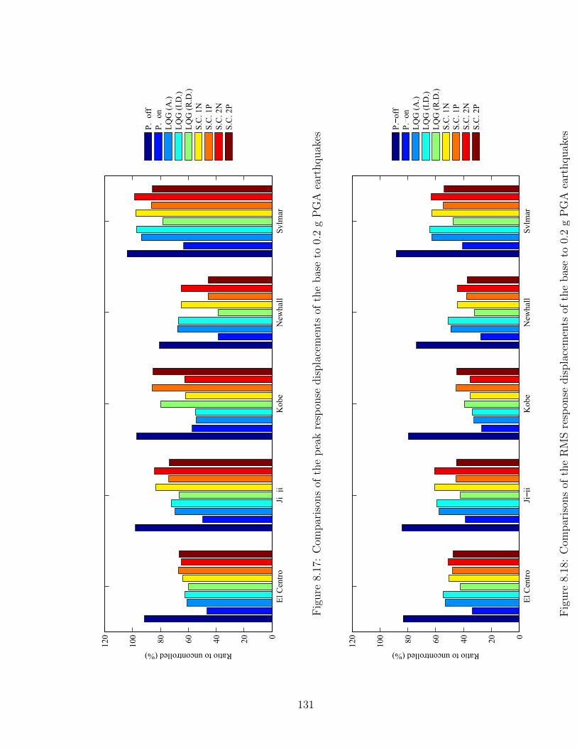
El
Cen
tro
Jiji
Kobe
New
hal
lS
ylm
ar0
20
40
60
80
100
120
Ratio to uncontrolled (%)
P.
off
P.
on
LQ
G (
A.)
LQ
G (
I.D
.)
LQ
G (
R.D
.)
S.C
. 1N
S.C
. 1P
S.C
. 2N
S.C
. 2P
Fig
ure
8.17
:C
ompar
ison
sof
the
pea
kre
spon
sedis
pla
cem
ents
ofth
ebas
eto
0.2
gP
GA
eart
hquak
es
El
Cen
tro
Jiji
Kobe
New
hal
lS
ylm
ar0
20
40
60
80
100
120
Ratio to uncontrolled (%)
P.
off
P.
on
LQ
G (
A.)
LQ
G (
I.D
.)
LQ
G (
R.D
.)
S.C
. 1N
S.C
. 1P
S.C
. 2N
S.C
. 2P
Fig
ure
8.18
:C
ompar
ison
sof
the
RM
Sre
spon
sedis
pla
cem
ents
ofth
ebas
eto
0.2
gP
GA
eart
hquak
es
131

El
Cen
tro
Jiji
Kobe
New
hal
lS
ylm
ar0
50
100
150
200
250
300
Ratio to uncontrolled (%)
P.
off
P.
on
LQ
G (
A.)
LQ
G (
I.D
.)
LQ
G (
R.D
.)
S.C
. 1N
S.C
. 1P
S.C
. 2N
S.C
. 2P
Fig
ure
8.19
:C
ompar
ison
sof
the
pea
kre
spon
seac
cele
rati
ons
ofth
ebas
eto
0.2
gP
GA
eart
hquak
es
El
Cen
tro
Jiji
Kobe
New
hal
lS
ylm
ar0
50
100
150
200
250
300
Ratio to uncontrolled (%)
P.
off
P.
on
LQ
G (
A.)
LQ
G (
I.D
.)
LQ
G (
R.D
.)
S.C
. 1N
S.C
. 1P
S.C
. 2N
S.C
. 2P
Fig
ure
8.20
:C
ompar
ison
sof
the
RM
Sre
spon
seac
cele
rati
ons
ofth
ebas
eto
0.2
gP
GA
eart
hquak
es
132

El
Cen
tro
Jiji
Kobe
New
hal
lS
ylm
ar0
50
100
150
200
250
300
Ratio to uncontrolled (%)
P.
off
P.
on
LQ
G (
A.)
LQ
G (
I.D
.)
LQ
G (
R.D
.)
S.C
. 1N
S.C
. 1P
S.C
. 2N
S.C
. 2P
Fig
ure
8.21
:C
ompar
ison
sof
the
pea
kre
spon
seac
cele
rati
ons
ofth
e6t
hfloor
to0.
2g
PG
Aea
rthquak
es
El
Cen
tro
Jiji
Kobe
New
hal
lS
ylm
ar0
50
100
150
200
250
300
Ratio to uncontrolled (%)
P.
off
P.
on
LQ
G (
A.)
LQ
G (
I.D
.)
LQ
G (
R.D
.)
S.C
. 1N
S.C
. 1P
S.C
. 2N
S.C
. 2P
Fig
ure
8.22
:C
ompar
ison
sof
the
RM
Sre
spon
seac
cele
rati
ons
ofth
e6t
hfloor
to0.
2g
PG
Aea
rthquak
es
133

El
Cen
tro
Jiji
Kobe
New
hal
lS
ylm
ar0
20
40
60
80
100
120
Ratio to uncontrolled (%)
P.
off
P.
on
LQ
G (
A.)
LQ
G (
I.D
.)
LQ
G (
R.D
.)
S.C
. 1N
S.C
. 1P
S.C
. 2N
S.C
. 2P
Fig
ure
8.23
:C
ompar
ison
sof
the
pea
kre
spon
sedis
pla
cem
ents
ofth
ebas
eto
0.5
gP
GA
eart
hquak
es
El
Cen
tro
Jiji
Kobe
New
hal
lS
ylm
ar0
20
40
60
80
100
120
Ratio to uncontrolled (%)
P.
off
P.
on
LQ
G (
A.)
LQ
G (
I.D
.)
LQ
G (
R.D
.)
S.C
. 1N
S.C
. 1P
S.C
. 2N
S.C
. 2P
Fig
ure
8.24
:C
ompar
ison
sof
the
RM
Sre
spon
sedis
pla
cem
ents
ofth
ebas
eto
0.5
gP
GA
eart
hquak
es
134

El
Cen
tro
Jiji
Kobe
New
hal
lS
ylm
ar0
50
100
150
200
250
300
Ratio to uncontrolled (%)
P.
off
P.
on
LQ
G (
A.)
LQ
G (
I.D
.)
LQ
G (
R.D
.)
S.C
. 1N
S.C
. 1P
S.C
. 2N
S.C
. 2P
Fig
ure
8.25
:C
ompar
ison
sof
the
pea
kre
spon
seac
cele
rati
ons
ofth
ebas
eto
0.5
gP
GA
eart
hquak
es
El
Cen
tro
Jiji
Kobe
New
hal
lS
ylm
ar0
50
100
150
200
250
300
Ratio to uncontrolled (%)
P.
off
P.
on
LQ
G (
A.)
LQ
G (
I.D
.)
LQ
G (
R.D
.)
S.C
. 1N
S.C
. 1P
S.C
. 2N
S.C
. 2P
Fig
ure
8.26
:C
ompar
ison
sof
the
RM
Sre
spon
seac
cele
rati
ons
ofth
ebas
eto
0.5
gP
GA
eart
hquak
es
135

El
Cen
tro
Jiji
Kobe
New
hal
lS
ylm
ar0
50
100
150
200
250
300
Ratio to uncontrolled (%)
P.
off
P.
on
LQ
G (
A.)
LQ
G (
I.D
.)
LQ
G (
R.D
.)
S.C
. 1N
S.C
. 1P
S.C
. 2N
S.C
. 2P
Fig
ure
8.27
:C
ompar
ison
sof
the
pea
kre
spon
seac
cele
rati
ons
ofth
e6t
hfloor
to0.
5g
PG
Aea
rthquak
es
El
Cen
tro
Jiji
Kobe
New
hal
lS
ylm
ar0
50
100
150
200
250
300
Ratio to uncontrolled (%)
P.
off
P.
on
LQ
G (
A.)
LQ
G (
I.D
.)
LQ
G (
R.D
.)
S.C
. 1N
S.C
. 1P
S.C
. 2N
S.C
. 2P
Fig
ure
8.28
:C
ompar
ison
sof
the
RM
Sre
spon
seac
cele
rati
ons
ofth
e6t
hfloor
to0.
5g
PG
Aea
rthquak
es
136

8.2.2 RTHS
The effectiveness of the smart base isolation system employing the MR damper isshown using RTHS. To compensate for time delays/lags, the feedforward-feedbackcompensator designed in Subsection 4.4.2 is employed. As input earthquakes, Kobe(1995, JMA station) and El Centro (1940, Imperial Valley) are considered. The Koberecord is scaled so that its peak ground acceleration (PGA) is 0.2 g and 0.5 g and thePGA of the El Centro record is scaled to 0.5 g.
The two semi-active control strategies, the LQG-based clipped-optimal controlwith acceleration weighting and the LQG-based clipped-optimal control with inter-story drift weighting, whose effectiveness were shown by the numerical simulationsare applied. In addition to these two semi-active controllers, the passive-off mode andthe passive-on mode cases are carried out.
The hystetetic force-displacement loops produced by the LQG-based clipped-optimal control with acceleration weighting and inter-story drift weighting subjectedto the three scaled earthquakes are depicted in Figures 8.29, 8.30, and 8.31, respec-tively. These hysteresis loops produced by the physical MR damper agrees with theones obtained by numerical simulation very well. As can be seen, the physical MRdamper produces clear pseudo-negative stiffness to 0.2 g PGA Kobe earthquake, whilefor the amplified earthquakes to 0.5g PGA, distinct properties of pseudo-negativestiffness are gone.
Tables 8.6 through 8.8 summarize the peak and root mean square (RMS) valuesof the response base displacements relative to the ground and absolute accelerationsat each floor for all cases. Figures 8.32 thorough 8.34 compare the normalized peakand RMS values based on the uncontrolled passive base isolation cases obtained fromsimulations. As can be seen in the tables and figures, the base isolation system with apassive-on mode or semi-actively controlled MR damper reduce both peak and RMSresponse and base displacement successfully compared to the uncontrolled passivebase isolation and passive-off mode MR damper cases. In terms of response acceler-ation, the risk of increasing peak acceleration can be found when the MR damper inpassive-on mode is applied. While the two semi-active controllers can reduce not onlybase displacement but also floor accelerations, the reductions in acceleration are notas large as in base displacement. Thus, considering both base displacement and flooraccelerations, the two designed semi-active controllers show better response reductionperformance than the three passive systems; the performance of the two semi-activecontrollers are quite similar.
An active base isolation study employing the same base-isolated building modelwas conducted by Chang and Spencer (2012). The active control system was ableto reduce the base displacement substantially, but this increased performance cameat the expense of a small increase in floor accelerations. In contrast, the semi-activecontrollers show reductions in both floor accelerations, especially at higher floors, andbase displacements. Considering that a semi-actively controlled system uses severalorders of magnitude less power than the actively controlled system, the MR dampercan be an attractive alternative for improved base isolation system performance.
137

−2 −1 0 1 2−400
−200
0
200
400
Displacement (in.)
MR
D f
orc
e (l
bf)
LQG−based C.O. control w/ A.
−2 −1 0 1 2−400
−200
0
200
400
Displacement (in.)
MR
D f
orc
e (l
bf)
LQG−based C.O. control w/ I.D.
Figure 8.29: Hysteresis loops produced by the physical MR damper to 0.2 g PGAKobe earthquake
−10 −5 0 5−400
−200
0
200
400
Displacement (in.)
MR
D f
orc
e (l
bf)
LQG−based C.O. control w/ A.
−10 −5 0 5−400
−200
0
200
400
Displacement (in.)
MR
D f
orc
e (l
bf)
LQG−based C.O. control w/ I.D.
Figure 8.30: Hysteresis loops produced by the physical MR damper to 0.5 g PGAKobe earthquake
−5 0 5−400
−200
0
200
400
Displacement (in.)
MR
D f
orc
e (l
bf)
LQG−based C.O. control w/ A.
−5 0 5−400
−200
0
200
400
Displacement (in.)
MR
D f
orc
e (l
bf)
LQG−based C.O. control w/ I.D.
Figure 8.31: Hysteresis loops produced by the physical MR damper to 0.5 g PGA ElCentro earthquake
138
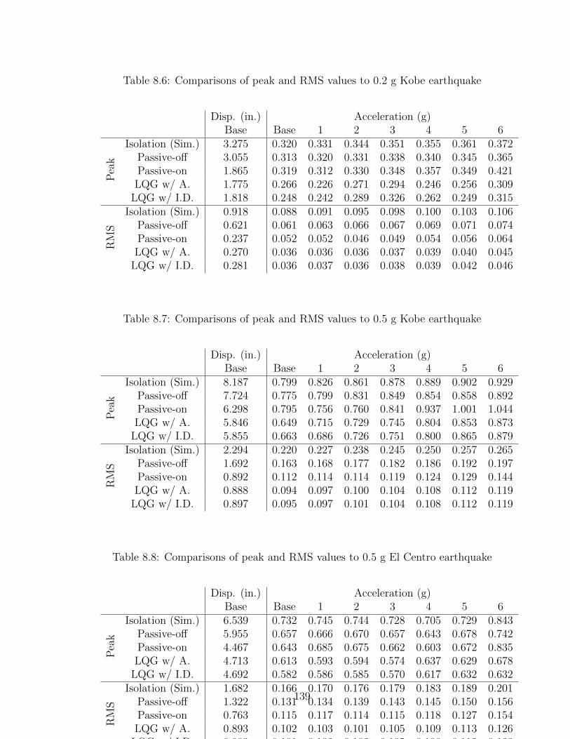
Table 8.6: Comparisons of peak and RMS values to 0.2 g Kobe earthquake
Disp. (in.) Acceleration (g)Base Base 1 2 3 4 5 6
Pea
k
Isolation (Sim.) 3.275 0.320 0.331 0.344 0.351 0.355 0.361 0.372Passive-off 3.055 0.313 0.320 0.331 0.338 0.340 0.345 0.365Passive-on 1.865 0.319 0.312 0.330 0.348 0.357 0.349 0.421LQG w/ A. 1.775 0.266 0.226 0.271 0.294 0.246 0.256 0.309
LQG w/ I.D. 1.818 0.248 0.242 0.289 0.326 0.262 0.249 0.315
RM
S
Isolation (Sim.) 0.918 0.088 0.091 0.095 0.098 0.100 0.103 0.106Passive-off 0.621 0.061 0.063 0.066 0.067 0.069 0.071 0.074Passive-on 0.237 0.052 0.052 0.046 0.049 0.054 0.056 0.064LQG w/ A. 0.270 0.036 0.036 0.036 0.037 0.039 0.040 0.045
LQG w/ I.D. 0.281 0.036 0.037 0.036 0.038 0.039 0.042 0.046
Table 8.7: Comparisons of peak and RMS values to 0.5 g Kobe earthquake
Disp. (in.) Acceleration (g)Base Base 1 2 3 4 5 6
Pea
k
Isolation (Sim.) 8.187 0.799 0.826 0.861 0.878 0.889 0.902 0.929Passive-off 7.724 0.775 0.799 0.831 0.849 0.854 0.858 0.892Passive-on 6.298 0.795 0.756 0.760 0.841 0.937 1.001 1.044LQG w/ A. 5.846 0.649 0.715 0.729 0.745 0.804 0.853 0.873
LQG w/ I.D. 5.855 0.663 0.686 0.726 0.751 0.800 0.865 0.879
RM
S
Isolation (Sim.) 2.294 0.220 0.227 0.238 0.245 0.250 0.257 0.265Passive-off 1.692 0.163 0.168 0.177 0.182 0.186 0.192 0.197Passive-on 0.892 0.112 0.114 0.114 0.119 0.124 0.129 0.144LQG w/ A. 0.888 0.094 0.097 0.100 0.104 0.108 0.112 0.119
LQG w/ I.D. 0.897 0.095 0.097 0.101 0.104 0.108 0.112 0.119
Table 8.8: Comparisons of peak and RMS values to 0.5 g El Centro earthquake
Disp. (in.) Acceleration (g)Base Base 1 2 3 4 5 6
Pea
k
Isolation (Sim.) 6.539 0.732 0.745 0.744 0.728 0.705 0.729 0.843Passive-off 5.955 0.657 0.666 0.670 0.657 0.643 0.678 0.742Passive-on 4.467 0.643 0.685 0.675 0.662 0.603 0.672 0.835LQG w/ A. 4.713 0.613 0.593 0.594 0.574 0.637 0.629 0.678
LQG w/ I.D. 4.692 0.582 0.586 0.585 0.570 0.617 0.632 0.632
RM
S
Isolation (Sim.) 1.682 0.166 0.170 0.176 0.179 0.183 0.189 0.201Passive-off 1.322 0.131 0.134 0.139 0.143 0.145 0.150 0.156Passive-on 0.763 0.115 0.117 0.114 0.115 0.118 0.127 0.154LQG w/ A. 0.893 0.102 0.103 0.101 0.105 0.109 0.113 0.126
LQG w/ I.D. 0.903 0.101 0.102 0.102 0.105 0.108 0.112 0.123
139

P off P on L (A.)L (I.D.)0
50
100
Rat
o t
o u
nco
ntr
oll
ed (
%)
(a)
P off P on L (A.)L (I.D.)0
50
100
Rat
o t
o u
nco
ntr
oll
ed (
%)
(b)
P off P on L (A.)L (I.D.)0
50
100
Rat
o t
o u
nco
ntr
oll
ed (
%)
(c)
P off P on L (A.)L (I.D.)0
50
100
Rat
o t
o u
nco
ntr
oll
ed (
%)
(d)
P off P on L (A.)L (I.D.)0
50
100
Rat
o t
o u
nco
ntr
oll
ed (
%)
(e)
P off P on L (A.)L (I.D.)0
50
100
Rat
o t
o u
nco
ntr
oll
ed (
%)
(f)
Figure 8.32: Reduction to 0.2 g Kobe earthquake; (a) Peak base displacement, (b)Peak base acceleration, (c) Peak 6th floor acceleration, (d) RMS base displacements,(e) RMS base acceleration, (f) RMS 6th floor acceleration
8.3 Summary
This chapter employs numerical simulation and RTHS to investigate a class of isola-tion systems that use semi-active control devices (i.e., smart base isolation). A six-story building was considered. The isolation system consisted of linear, low-dampingisolators, combined with a magnetorheological (MR) fluid damper. In RTHS, thesmart isolated building was substructured, such that the building was modeled com-putationally, whereas the MR damper was tested physically. This smart base isolationsystem is found to reduce base displacements and floor accelerations better than thepassive counterparts. Improvements were also demonstrated over the active isolationsystem, without the need for large external power sources.
The versatility of the hysteresis loops produced by the LQG-based clipped-optimalcontrollers and the proposed simple controllers was shown through numerical simu-lation and RTHS, as well. However, in seismic performance, the proposed simplecontrollers were not comparable to the LQG-based clipped-optimal controllers, espe-cially in the upper floors.
140

P off P on L (A.)L (I.D.)0
50
100
Rat
o t
o u
nco
ntr
oll
ed (
%)
(a)
P off P on L (A.)L (I.D.)0
50
100R
ato t
o u
nco
ntr
oll
ed (
%)
(b)
P off P on L (A.)L (I.D.)0
50
100
Rat
o t
o u
nco
ntr
oll
ed (
%)
(c)
P off P on L (A.)L (I.D.)0
50
100
Rat
o t
o u
nco
ntr
oll
ed (
%)
(d)
P off P on L (A.)L (I.D.)0
50
100
Rat
o t
o u
nco
ntr
oll
ed (
%)
(e)
P off P on L (A.)L (I.D.)0
50
100R
ato t
o u
nco
ntr
oll
ed (
%)
(f)
Figure 8.33: Reduction to 0.5 g Kobe earthquake; (a) Peak base displacement, (b)Peak base acceleration, (c) Peak 6th floor acceleration, (d) RMS base displacements,(e) RMS base acceleration, (f) RMS 6th floor acceleration
141

P off P on L (A.)L (I.D.)0
50
100
Rat
o t
o u
nco
ntr
oll
ed (
%)
(a)
P off P on L (A.)L (I.D.)0
50
100R
ato t
o u
nco
ntr
oll
ed (
%)
(b)
P off P on L (A.)L (I.D.)0
50
100
Rat
o t
o u
nco
ntr
oll
ed (
%)
(c)
P off P on L (A.)L (I.D.)0
50
100
Rat
o t
o u
nco
ntr
oll
ed (
%)
(d)
P off P on L (A.)L (I.D.)0
50
100
Rat
o t
o u
nco
ntr
oll
ed (
%)
(e)
P off P on L (A.)L (I.D.)0
50
100R
ato t
o u
nco
ntr
oll
ed (
%)
(f)
Figure 8.34: Reduction to 0.5 g El Centro earthquake; (a) Peak base displacement, (b)Peak base acceleration, (c) Peak 6th floor acceleration, (d) RMS base displacements,(e) RMS base acceleration, (f) RMS 6th floor acceleration
142

Chapter 9
CONCLUSIONS AND FUTURE STUDIES
9.1 Conclusions
In this report, the possibility of semi-active control strategies have been explored, andtheir effectiveness has been verified experimentally for seismically excited buildings.The properties of the hysteretic force-displacement loops produced by semi-activelycontrolled MR dampers and their seismic performance were investigated.
A review of literature in the area of structural control technologies was first pre-sented with a focus on outrigger damping systems and hybrid base-isolation systems.Literature related to real-time hybrid simulation was reviewed as well. Also, ba-sic background on modern control theories which are necessary to design active andsemi-active controllers was introduced, and the servo-hydraulic system model, theMR damper model, and the model-based compensators for RTHS were developed.
The nature of the hysteretic behavior of the active control forces produced bythe widely employed LQG-based acceleration feedback control strategies was inves-tigated, revealing the relationship between the properties of the control forces andthe response. Numerical simulation studies carried out on one-story and three-storybuildings with active bracing show that the LQG-based algorithms are quite versatileand can produce controllers with a variety of behaviors. The effectiveness of nega-tive stiffness control force was shown through numerical studies. Additionally, thenumerical results demonstrated that the presented LQG-based acceleration feedbackcontrol had performance comparable to the LQR in the presented SDOF and 3DOFbuilding models.
Following the hysteretic behavior of the active control forces and the seismic re-sponses, hysteresis loops produced by the semi-actively controlled MR damper wereinvestigated. Two new model-free semi-active control algorithms for controllabledampers were proposed. One of the algorithms needs only the directions of the dis-placement and the velocity of the damper to decide the input current to the damper.The other one needs the directions of only the displacement and the output force ofthe damper. Thus, the structure model and a number of sensors are not requiredto implement the proposed algorithms. Moreover, this research demonstrated thatthe proposed controllers can produce versatile hysteresis control force loops throughnumerical simulations on the scaled three-story building model with the MR damper.Also, the effectiveness of hysteresis loops having pseudo-negative stiffness was veri-fied. Additionally, the numerical results showed that the proposed two algorithmsproducing pseudo-negative stiffness had performance comparable to the LQG-basedclipped-optimal controllers, which need the accurate structure model and more sen-sors.
143
To show the effectiveness of the semi-active strategies on complicated structuresexperimentally, the efficacy of the model-based compensator for RTHS on a MDOFstructure was verified through a high-rise building model with an outrigger dampingsystem. Through this research, the following general conclusions were drawn: a)RTHS worked when all modes of the structure were lightly damped, demonstrating therobustness of the actuator controller without the need for adding numerical damping;b) the actuator control strategy used in this study demonstrated stable and accurateresults in MDOF structural systems; c) RTHS can be employed for validation ofstructural control algorithms; d) RTHS provides an effective means for assessing thesystem performance of rate-dependent components in complex structures.
Also, this study showed that MR dampers can be employed effectively in outrig-ger damping systems using passive-on mode and semi-active controllers. The MRdamper’s restoring force can be simulated quite well by the proposed MR dampermodel for the two earthquake records; however, differences are still present. In par-ticular, discrepancies between simulations and RTHSs were found in the base shear.Moreover, the physical specimen contains no modeling errors, while it is subject toexperimental error such as magnitude and time delay. The numerical model providesa good verification tool for RTHS; however it is subject to numerical errors, is onlyvalid within the range of behavior for which the model is calibrated, and cannot fullyrepresent the complex specimen behavior. Thus, the importance of combining RTHSwith numerical simulation to ensure accurate results was demonstrated.
A class of isolation systems that use semi-active control devices (i.e., smart baseisolation) was investigated through numerical simulation and RTHS as well. In thisstudy, a base-isolated six-story building was considered. The isolation system con-sisted of linear, low-damping isolators, combined with a MR damper. In RTHS, thesmart isolated building was substructured, such that the building was modeled com-putationally, whereas the MR damper was tested physically. This smart base isolationsystem is found to reduce base displacements and floor accelerations better than thepassive counterparts. Improvements were also demonstrated over the active isolationsystem, without the need for large external power sources.
On the base-isolated six-story building model, the versatility of the hysteresisloops produced by the LQG-based clipped-optimal controllers and the proposed sim-ple controllers was shown through numerical simulation and RTHS, as well. However,in seismic performance, the proposed simple controllers were not comparable to theLQG-based clipped-optimal controllers, especially in the upper floors. This result im-plies that the proposed simple controllers are not suitable for complicated structures.
In conclusion, this report provided the hysteresis behavior and the seismic perfor-mance of semi-active control strategies on buildings and showed the strong potentialfor practical use to mitigate seismic damage. However, some disappointing resultswere also observed.
144
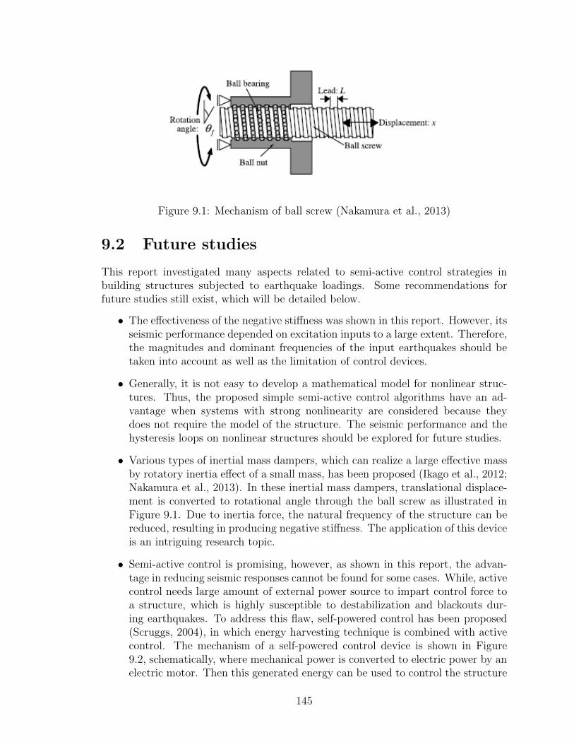
Figure 9.1: Mechanism of ball screw (Nakamura et al., 2013)
9.2 Future studies
This report investigated many aspects related to semi-active control strategies inbuilding structures subjected to earthquake loadings. Some recommendations forfuture studies still exist, which will be detailed below.
• The effectiveness of the negative stiffness was shown in this report. However, itsseismic performance depended on excitation inputs to a large extent. Therefore,the magnitudes and dominant frequencies of the input earthquakes should betaken into account as well as the limitation of control devices.
• Generally, it is not easy to develop a mathematical model for nonlinear struc-tures. Thus, the proposed simple semi-active control algorithms have an ad-vantage when systems with strong nonlinearity are considered because theydoes not require the model of the structure. The seismic performance and thehysteresis loops on nonlinear structures should be explored for future studies.
• Various types of inertial mass dampers, which can realize a large effective massby rotatory inertia effect of a small mass, has been proposed (Ikago et al., 2012;Nakamura et al., 2013). In these inertial mass dampers, translational displace-ment is converted to rotational angle through the ball screw as illustrated inFigure 9.1. Due to inertia force, the natural frequency of the structure can bereduced, resulting in producing negative stiffness. The application of this deviceis an intriguing research topic.
• Semi-active control is promising, however, as shown in this report, the advan-tage in reducing seismic responses cannot be found for some cases. While, activecontrol needs large amount of external power source to impart control force toa structure, which is highly susceptible to destabilization and blackouts dur-ing earthquakes. To address this flaw, self-powered control has been proposed(Scruggs, 2004), in which energy harvesting technique is combined with activecontrol. The mechanism of a self-powered control device is shown in Figure9.2, schematically, where mechanical power is converted to electric power by anelectric motor. Then this generated energy can be used to control the structure
145
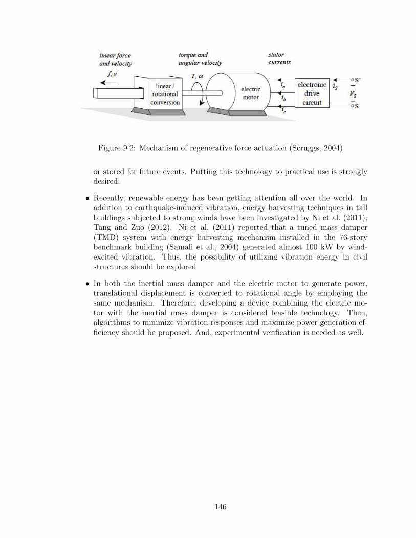
Figure 9.2: Mechanism of regenerative force actuation (Scruggs, 2004)
or stored for future events. Putting this technology to practical use is stronglydesired.
• Recently, renewable energy has been getting attention all over the world. Inaddition to earthquake-induced vibration, energy harvesting techniques in tallbuildings subjected to strong winds have been investigated by Ni et al. (2011);Tang and Zuo (2012). Ni et al. (2011) reported that a tuned mass damper(TMD) system with energy harvesting mechanism installed in the 76-storybenchmark building (Samali et al., 2004) generated almost 100 kW by wind-excited vibration. Thus, the possibility of utilizing vibration energy in civilstructures should be explored
• In both the inertial mass damper and the electric motor to generate power,translational displacement is converted to rotational angle by employing thesame mechanism. Therefore, developing a device combining the electric mo-tor with the inertial mass damper is considered feasible technology. Then,algorithms to minimize vibration responses and maximize power generation ef-ficiency should be proposed. And, experimental verification is needed as well.
146

REFERENCES
Abdel-Rohman, M. (1984). “Optimal control of tall buildings by appendages.” Jour-nal of Structural Engineering, 110(5), 937–947.
Abdel-Rohman, M. and Leipholz, H. (1983). “Active control of tall buildings.” Jour-nal of Structural Engineering, 109(3), 628–645.
Akbay, Z. and Aktan, H. (1990). “Intelligent energy dissipation devices.” Proceedingsof the fourth U.S. National Conference on Earthquake Engineering, Vol. 3, 427–435.
Akbay, Z. and Aktan, H. (1991). “Actively regulated friction slip devices.” Proceedingsof the sixth Canadian Conference on Earthquake Engineering, 363–374.
Berton, S. and Bolander, J. E. (2005). “Amplification system for supplemental damp-ing devices in seismic applications.” Journal of Structural Engineering, 131(6), 979–983.
Blakeborough, A., Williams, M. S., Darby, A., and Williams, D. M. (2001). “Thedevelopment of real-time substructure testing.” Philosophical Transactions of theRoyal Society A - Mathematical, Physical and Engineering Sciences, 359, 1869.
Carlson, J. (1994). “The promise of controllable fluids.” Proceedings of Actuator 94,266–270.
Carlson, J., Catanzarite, D., and St. Clair, K. (1996). “Commercial magneto-rheological fluid devices.” International Journal of Modern Physics B, 10(23 &24), 2857–2865.
Carlson, J. and Spencer, Jr., B. F. (1996). “Magneto-rheological fluid dampers forsemi-active seismic control.” Proceedings of the 3rd International Conference onMotion and Vibration Control, 35–40.
Carlson, J. and Weiss, K. D. (1994). “A growing attraction to magnetic fluids.”Machine Design, (August), 61–64.
Carrion, J. E. and Spencer, Jr., B. F. (2007). “Model-based strategies for real-timehybrid testing.” Report No. 6, Department of Civil and Environmental Engineering,University of Illinois at Urbana-Champaign (Dec.).
Casciati, F., Faravelli, L., and Venini, P. (1993). A Neural-Network Performance-Function Selection in Active Structural Control. Dept. of Civil Engineering, Schoolof Engineering, University of Southern California.
147

Chameau, J., Reed, D., and Yao, J. (1991). “Intelligent systems in civil engineering.”Proceedings of the International Fussy Systems Association, Brussels, Belgium.
Chang, C.-M., Park, K.-S., Mullenix, A., and Spencer, Jr., B. F. (2008). “Semiactivecontrol strategy for a phase ii smart base isolated benchmark building.” StructuralControl and Health Monitoring, 15(5), 673–696.
Chang, C. M. and Spencer, Jr., B. F. (2012). “Multi-axial active isolation for seismicprotection of buildings.” Report No. 30, Department of Civil and EnvironmentalEngineering, University of Illinois at Urbana-Champaign (May).
Chang, C. M., Wang, Z., Spencer, Jr., B. F., and Chen, Z. (2013). “Semi-activedamped outriggers for seismic protection of high-rise buildings.” Smart Structuresand Systems, 11(5), 435–451.
Chang, J. C. and Soong, T. T. (1980). “Structural control using active tuned massdampers.” Journal of the Engineering Mechanics Division, 106(6), 1091–1098.
Charles, J. (2006). “Application of damping in high-rise buildings.” M.S. thesis,M.I.T., M.I.T.
Chopra, A. (2007). Dynamics of Structures: Theory and Applications to EarthquakeEngineering. Pearson/Prentice Hall.
Constantinou, M. C., Symans, M. D., Tsopelas, P., and Taylor, D. P. (1993). “Fluidviscous dampers in applications of seismic energy dissipation and seismic isolation.”Proceedings of ATC 17-1 seminar on seismic isolation, passive energy dissipation,and active control, 581–592.
Constantinou, M. C., Tsopelas, P., Hammel, W., and Sigaher, A. N. (2001). “Toggle-brace-damper seismic energy dissipation systems.” Journal of Structural Engineer-ing, 127(2), 105–112.
Darby, A. P., Blakeborough, A., and Williams, M. S. (2001). “Improved controlalgorithm for real-time substructure testing.” Earthquake Engineering & StructuralDynamics, 30(3), 431–448.
Den Hartog, J. (1956). Mechanical Vibrations. Read Books.
Dyke, S. J., Spencer, Jr., B. F., Quast, P., Kaspari, D. C., and Sain, M. K. (1996a).“Implementation of an active mass driver using acceleration feedback control.”Computer-Aided Civil and Infrastructure Engineering, 11(5), 305–323.
Dyke, S. J., Spencer, Jr., B. F., Quast, P., and Sain, M. K. (1995). “Role of control-structure interaction in protective system design.” Journal of Engineering Mechan-ics, 121(2), 322–338.
Dyke, S. J., Spencer, Jr., B. F., Quast, P., Sain, M. K., Kaspari, Jr., D. C., andSoong, T. T. (1996b). “Acceleration feedback control of mdof structures.” Journalof Engineering Mechanics, 122(9), 907–918.
148
Dyke, S. J., Spencer, Jr., B. F., Sain, M. K., and Carlson, J. D. (1996c). “Modelingand control of magnetorheological dampers for seismic response reduction.” SmartMaterials and Structures, 5(5), 565–575.
Dyke, S. J., Spencer, Jr., B. F., Sain, M. K., and Carlson, J. D. (1996d). “A newsemi-active control device for seismic response reduction.” Proceedings of the 11thASCE Engineering Mechanics Specialty Conference, 886–889.
Ehrgott, R. and Masri, S. (1994). “Structural control applications of an electrorhe-ological device.” Proceedings of the International Workshop on Structural Control,Dept. of Civil Engineering, School of Engineering, University of Southern Califor-nia, 115–129. USC publication No. CE-9311.
Feng, M. (1993). “Application of hybrid sliding isolation system to buildings.” Journalof Engineering Mechanics, 119(10), 2090–2108.
Feng, Q. and Shinozuka, M. (1990). “Use of a variable damper for hybrid controlof bridge response under earthquake.” Proceedings of the U.S. National Workshopon Structural Control Research, Dept. of Civil Engineering, School of Engineering,University of Southern California, 107–112. USC publication No. CE-9013.
Fur, L., Yang, H., and Ankireddi, S. (1996). “Vibration control of tall buildings underseismic and wind loads.” Journal of Structural Engineering, 122(8), 948–957.
Furuta, H., Okanan, H., Kaneyoshi, M., and Tanaka, H. (1994). “Application ofgenetic algorithms to self-tuning of fuzzy active control for structural vibration.”Proceedings of the first World Conference on Structural Control, WP1:3–12.
Gattulli, V., Lin, R., and Soong, T. (1994). “Nonlinear control laws for enhancementof structural control effectiveness.” Proceedings of 5th U.S. National Conference forEarthquake Engineering, Chicago, IL, 971–980.
Gavin, H., Hose, Y., and Hanson, R. (1994a). “Design and control of electrorheo-logical dampers.” Proceedings of the 1st World Conference on Structural Control,Pasadena, CA, WP3:83–92.
Gavin, H., Ortiz, D., and Hanson, R. (1994b). “Testing and modeling of a prototypeer damper for seismic structural response control.” Proceedings of the InternationalWorkshop on Structural Control, Dept. of Civil Engineering, School of Engineering,University of Southern California, 166–180. USC publication No. CE-9311.
Gordaninejad, F., Ray, A., and Bindu, R. (1994). “Vibration control of structuresusing hybrid er/viscous dampers.” Proceedings of the 1st World Conference onStructural Control, Pasadena, CA, TA2:41–49.
Hakuno, M., Shidawara, M., and Hara, T. (1969). “Dynamic destructive test of acantilever beam controlled by an analog-computer.” Journal of JSCE, 171, 1–9 (inJapanese).
149
Haroun, M., Pires, J., and Won, A. (1994). “Active orifice control in hybrid liq-uid dampers.” Proceedings of the 1st World Conference on Structural Control,Pasadena, CA, FA1:69–78.
Horiuchi, T., Nakagawa, M., Sugano, M., and Konno, T. (1996). “Development of areal-time hybrid experimental system with actuator delay compensation.” Proceed-ings of the 11th World Conference of Earthquake Engineering. No. 660.
Housner, G., Bergman, L., Caughey, T., Chassiakos, A., Claus, R., Masri, S., Skelton,R., Soong, T., Spencer, Jr., B., and Yao, J. (1997). “Structural control: Past,present, and future.” Journal of Engineering Mechanics, 123(9), 897–971.
Iemura, H., Igarashi, A., Pradono, M. H., and Kalantari, A. (2006). “Negative stiffnessfriction damping for seismically isolated structures.” Structural Control and HealthMonitoring, 13(2-3), 775–791.
Iemura, H., Igarashi, A., Toyooka, A., and Higuchi, M.and Kouchiyama, O.(2010). “Theoretical, numerical and experimental verification of negative stiff-ness dampers.” Proceedings of the 5th World Conference on Structural Control andMonitoring, Tokyo, Japan.
Iemura, H., Igarashi, A., Toyooka, A., Kouchiyama, O., and Higuchi, M. (2008).“Seismic response control with innovative negative stiffness dampers.” Proceedingsof the 14th World Conference on Structural Control and Monitoring, Beijing, China.
Iemura, H. and Pradono, M. H. (2002). “Passive and semi-active seismic responsecontrol of a cable-stayed bridge.” Journal of Structural Control, 9(3), 189–204.
Iemura, H. and Pradono, M. H. (2005). “Simple algorithm for semi-active seismicresponse control of cable-stayed bridges.” Earthquake Engineering & StructuralDynamics, 34(4-5), 409–423.
Iemura, H. and Pradono, M. H. (2009). “Advances in the development of pseudo-negative-stiffness dampers for seismic response control.” Structural Control andHealth Monitoring, 16(7-8), 784–799.
Ikago, K., Saito, K., and Inoue, N. (2012). “Seismic control of single-degree-of-freedomstructure using tuned viscous mass damper.” Earthquake Engineering & StructuralDynamics, 41(3), 453–474.
Ikhouane, F., Rabeh, A., and Giri, F. (1997). “Transient performance analysis inrobust nonlinear adaptive control.” Systems & Control Letters, 31(1), 21 – 31.
Inaudy, J. and Kelly, J. (1990). “Active isolation.” Proceedings of the U.S. NationalWorkshop on Structural Control Research, Los Angeles, CA, 125–130.
Infanti, S., Robinson, J., and Smith, R. (2008). “Viscous dampers for high-rise build-ings.
150

Jansen, L. and Dyke, S. (2000). “Semiactive control strategies for mr dampers: Com-parative study.” Journal of Engineering Mechanics, 126(8), 795–803.
Kalman, R. E. (1960). “A new approach to linear filtering and prediction problems.”Journal of Basic Engineering, 82(1), 35–45.
Kalman, R. E. and Bucy, R. S. (1961). “New results in linear filtering and predictiontheory.” Journal of Basic Engineering, 83(1), 95–108.
Kamagata, S. and Kobori, T. (1994). “Autonomous adaptive control of active vari-able stiffness system for seismic ground motion.” Proceedings of the First WorldConference on Structural Control, Pasadena, CA, TA4:33–42.
Kannan, S., Uras, H. M., and Aktan, H. M. (1995). “Active control of building seismicresponse by energy dissipation.” Earthquake Engineering & Structural Dynamics,24(5), 747–759.
Kareem, A., Kijewski, T., and Y., T. (1999). “Mitigation of motion of tall buildingswith recent applications.” Wind and Structures, 2(3), 201–251.
Karimi, H. R., Zapateiro, M., and Luo, N. (2009). “Vibration control of base-isolatedstructures using mixed h2/h output-feedback control.” Proceedings of the Institu-tion of Mechanical Engineers, Part I: Journal of Systems and Control Engineering,223(6), 809–820.
Karnopp, D., Crosby, M. J., and Harwood, R. A. (1974). “Vibration control usingsemi-active force generators.” Journal of Engineering for Industry, 96(2), 619–626.
Kelly, J. (1997). Earthquake-resistant design with rubber. Springer.
Kelly, J. M., Leitmann, G., and Soldatos, A. G. (1987). “Robust control of base-isolated structures under earthquake excitation.” Journal of Optimization Theoryand Applications, 53, 159–180.
Khalil, H. (2002). Nonlinear Systems. Prentice Hall PTR.
Kim, S. B., Spencer, J. B. F., and Yun, C.-B. (2005). “Frequency domain identificationof multi-input, multi-output systems considering physical relationships betweenmeasured variables.” Journal of Engineering Mechanics, 131(5), 461–472.
Kobori, T. (1990). “Technology development and forecast of dynamical intelligentbuilding (d.i.b).” Journal of Intelligent Material systems and structures, 1(4), 391–407.
Kobori, T. (1996). “Future direction on research and development of seismic-response-controlled structures.” Computer-Aided Civil and Infrastructure Engineering, 11(5),297–304.
151

Lee-Glauser, G., Ahmadi, G., and Horta, L. (1997). “Integrated passive/active vibra-tion absorber for multistory buildings.” Journal of Structural Engineering, 123(4),499–504.
Leitmann, G. (1994). “Semiactive control for vibration attenuation.” Journal of In-telligent Material Systems and Structures, 5(6), 841–846.
Liberzon, D. (2012). Calculus of Variations and Optimal Control Theory: A ConciseIntroduction. Princeton University Press.
Lin, P. Y., Roschke, P. N., and Loh, C. H. (2007). “Hybrid base-isolation with magne-torheological damper and fuzzy control.” Structural Control and Health Monitoring,14(3), 384–405.
Loh, C.-H. and Chao, C.-H. (1996). “Effectiveness of active tuned mass damper andseismic isolation on vibration control of multi-storey building.” Journal of Soundand Vibration, 193(4), 773 – 792.
Loh, C.-H. and Ma, M.-J. (1996). “Control of seismically excited building structuresusing variable damper systems.” Engineering Structures, 18(4), 279 – 287.
Lou, J. Y. K., Lutes, L. D., and Li, J. J. (1994). “Active tuned liquid damper forstructural control.” Proceedings of the 1st World Conference on Structural Control,Pasadena, CA, TP1:70–79.
Luo, N., Rodellar, J., la Sen, M., and Vehi, J. (2000). “Output feedback sliding modecontrol of base isolated structures.” Journal of the Franklin Institute, 337(5), 555– 577.
Luo, N., Rodellar, J., Villamizar, R., and Vehi, J. (2003). “Robust control law for afriction-based semiactive controller of a two-span bridge.” Proc. SPIE.
Luo, N., Villamizar, R., and Vehi, J. (2004). “Quantitative feedback theory (qft):application to structural control.” Proceedings of China-Japan-US Symposium onHealth Monitoring and Control of Structures, Dailan, China.
Luo, N., Villamizar, R., Vehi, J., and Dyke, S. (2006). “Semiactive backsteppingcontrol for vibration attenuation in structures equipped with magnetorheologicalactuators.” Computer Aided Control System Design, 2006 IEEE International Con-ference on Control Applications, 2006 IEEE International Symposium on IntelligentControl, 2006 IEEE, 1091 –1096 (oct.).
Makris, N. (1997). “Rigidityplasticityviscosity: Can electrorheological dampers pro-tect base-isolated structures from near-source ground motions?.” Earthquake En-gineering & Structural Dynamics, 26(5), 571–591.
Makris, N., Burton, S., Hill, D., and Jordan, M. (1996). “Analysis and design of erdamper for seismic protection of structures.” Journal of Engineering Mechanics,122(10), 1003–1011.
152
Makris, N., Hill, D., Burton, S., and Jordan, M. (1995). “Electrorheological fluiddamper for seismic protection of structures.” 184–194.
MATLAB (2013). The Math Works, Inc., Natick, MA.
McClamroch, N. and Gavin, H. (1995). “Closed loop structural control using elec-trorheological dampers.” American Control Conference, 1995. Proceedings of the,Vol. 6, 4173–4177 (jun).
McClamroch, N., Oritz, D., Gavin, H., and Hanson, R. (1994). “Electrorheologicaldampers and semi-active structural control.” Decision and Control, 1994., Proceed-ings of the 33rd IEEE Conference on, Vol. 1, 97–102.
Merritt, H. (1967). Hydraulic Control Systems. Wiley.
Moon, S., Bergman, L., and Voulgaris, P. (2003). “Sliding mode control of cable-stayed bridge subjected to seismic excitation.” Journal of Engineering Mechanics,129(1), 71–78.
Nagarajaiah, S. and Narasimhan, S. (2006). “Smart base-isolated benchmark build-ing. part ii: phase i sample controllers for linear isolation systems.” StructuralControl and Health Monitoring, 13(2-3), 589–604.
Nagarajaiah, S. and Narasimhan, S. (2007). “Seismic control of smart base isolatedbuildings with new semiactive variable damper.” Earthquake Engineering & Struc-tural Dynamics, 36(6), 729–749.
Nagarajaiah, S., Reinhorn, A., Constantinou, M., Taylor, D., and Pasala, D. (2010).“Adaptive negative stiffness: A new structural modification approach for seismicprotection.” Proceedings of the 5th World Conference on Structural Control andMonitoring, Tokyo, Japan.
Nakamura, Y., Fukukita, A., Tamura, K., Yamazaki, I., Matsuoka, T., Hiramoto, K.,and Sunakoda, K. (2013). “Seismic response control using electromagnetic inertialmass dampers.” Earthquake Engineering & Structural Dynamics.
Nakashima, M., Kato, H., and Takaoka, E. (1992). “Development of real-time pseudodynamic testing.” Earthquake Engineering & Structural Dynamics, 21(1), 79–92.
Nakashima, M. and Masaoka, N. (1999). “Real-time on-line test for MDOF systems.”Earthquake Engineering & Structural Dynamics, 28(4), 393–420.
Narasimhan, S., Nagarajaiah, S., and Johnson, E. A. (2008). “Smart base-isolatedbenchmark building part iv: Phase ii sample controllers for nonlinear isolationsystems.” Structural Control and Health Monitoring, 15(5), 657–672.
Ni, T., Zuo, L., and Kareem, A. (2011). “Assessment of energy potential and vibrationmitigation of regenerative tuned mass dampers on wind excited tall buildings.”Proceedings of the 23rd Biennial Conference on Mechanical Vibration and Noise,333–342.
153

Nishimura, H. and Kojima, A. (1998). “Active vibration isolation control for amulti-degree-of-freedom structure with uncertain base dynamics.” JSME interna-tional journal. Series C, Mechanical systems, machine elements and manufacturing,41(1), 37 – 45.
Patten, W., Kuo, C., He, Q., Liu, L., and Sack, R. (1994a). “Seismic structuralcontrol via hydraulic semiactive vibration dampers (savd).” Proceedings of the 1stWorld Conference on Structural Control, Pasadena, CA, FA2:83–92.
Patten, W., Kuo, C., He, Q., Liu, L., and Sack, R. (1994b). “Suppression of vehicle-induced bridge vibration via hydraulic semiactive vibration dampers.” Proceedingsof the 1st World Conference on Structural Control, Pasadena, CA, FA1:30–38.
Phillips, B. M. and Spencer, Jr., B. F. (2012). “Model-based framework for real-time dynamic structural performance evaluation.” Report No. 31, Department ofCivil and Environmental Engineering, University of Illinois at Urbana-Champaign(Aug.).
Pu, J. and Kelly, J. (1991). “Active control and seismic isolation.” Journal of Engi-neering Mechanics, 117(10), 2221–2236.
Rabinow, J. (1948). “The magnetic fluid clutch.” American Institute of ElectricalEngineers, Transactions of the, 67(2), 1308 –1315.
Ramallo, J., Johnson, E., and Spencer, Jr., B. F. (2002). “smart base isolationsystems.” Journal of Engineering Mechanics, 128(10), 1088–1099.
Ramallo, J. C., Johnson, E. A., Spencer, Jr., B. F., and Sain, M. K. (1999). “Semi-active building base isolation.” American Control Conference, 1999. Proceedings ofthe 1999, Vol. 1, 515–519 vol.1.
Reinhorn, A., Soong, T., Lin, R., Wang, Y., Fukuo, Y., Abe, H., and Nakai, M.(1989). “1:4 scale model studies of active tendon systems and active mass dampersfor aseismic protection.” Report no., National Center for Earthquake EngineeringResearch, State University of New York at Buffalo, Buffalo, NY.
Reinhorn, A. M., Li, C., and Constantinou, M. C. (1995). “Experimental and an-alytical investigation of seismic retrofit of structures with supplemental damping: Part.1 - fluid viscous damping devices.” Report no., National Center for Earth-quake Engineering Research, State University of New York at Buffalo, Buffalo, NY(Jan.).
Riley, M., Reinhorn, A., and Nagarajaiah, S. (1998). “Implementation issues andtesting of a hybrid sliding isolation system.” Engineering Structures, 20(3), 144 –154.
154
Sahasrabudhe, S. and Nagarajaiah, S. (2005). “Effectiveness of variable stiffness sys-tems in base-isolated bridges subjected to near-fault earthquakes: An experimen-tal and analytical study.” Journal of Intelligent Material Systems and Structures,16(9), 743–756.
Samali, B., Kwok, K., Wood, G., and Yang, J. (2004). “Wind tunnel tests for wind-excited benchmark building.” Journal of Engineering Mechanics, 130(4), 447–450.
Scruggs, J. T. (2004). “Structural control using regenerative force actuation net-works.” Ph.D. thesis, California Institute of Technology, Pasadena, CA.
Shook, D., Lin, P.-Y., Lin, T.-K., and Roschke, P. N. (2007). “A comparative studyin the semi-active control of isolated structures.” Smart Materials and Structures,16(4), 1433–1446.
Shoureshi, R., Bell, M., and Wheeler, M. (1994). “Neural-based intelligent con-trol of structures.” Proceedings of the 1st World Conference on Structural Control,Pasadena, CA, FP4:3–11.
Sigaher, A. N. and Constantinou, M. C. (2003). “Scissor-jack-damper energy dissi-pation system.” Earthquake Spectra, 19(1), 133–158.
SIMULINK (2013). The Math Works, Inc., Natick, MA.
Skelton, R. E. (1988). Dynamic Systems Control. John Wiley and Sons.
Smith, B. S. and Salim, I. (1981). “Parameter study of outrigger-braced tall buildingstructures.” Journal of the Structural Division, 107(10), 2001–2014.
Smith, R. J. and Willford, M. R. (2007). “The damped outrigger concept for tallbuildings.” The Structural Design of Tall and Special Buildings, 16(4), 501–517.
Soong, T. and Costantinou, C. (1995). Passive and Active Structural Vibration Con-trol in Civil Engineering. CISM INTERNATIONAL CENTRE FOR MECHANI-CAL SCIENCES COURSES AND LECTURES. Springer Verlag.
Soong, T. T. and Reinhorn, A. M. (1993). “Case studies of active control and imple-mentational issues.” Proceedings of ATC-17-1 Seminar of Seismic Isolation, Pas-sive Energy Dissipation, and Active Control, Vol. 2, 701–713.
Soong, T. T. and Skinner, G. T. (1981). “Experimental study of active structuralcontrol.” Journal of the Engineering Mechanics Division, 107(6), 1057–1067.
Spencer, Jr., B. F., Dyke, S. J., Sain, M. K., and Carlson, J. D. (1997). “Phenomeno-logical model for magnetorheological dampers.” Journal of Engineering Mechanics,123(3), 230–238.
Spencer, Jr., B. F., Johnson, E. A., and Ramallo, J. C. (2000). “Smart isolationfor seismic control.” JSME international journal. Series C, Mechanical systems,machine elements and manufacturing, 43(3), 704 – 711.
155

Spencer, Jr., B. F. and Nagarajaiah, S. (2003). “State of the art of structural control.”Journal of Structural Engineering, 129(7), 845–856.
Spencer, Jr., B. F., Suhardjo, J., and Sain, M. (1994). “Frequency domain opti-mal control strategies for aseismic protection.” Journal of Engineering Mechanics,120(1), 135–158.
Stengel, R. (1986). Stochastic optimal control: theory and application. Wiley-Interscience publication. Wiley.
Stengel, R. (1994). Optimal control and estimation. Dover Publications.
Suhardjo, J., Spencer, Jr., B. F., and Kareem, A. (1992). “Frequency domain opti-mal control of windexcited buildings.” Journal of Engineering Mechanics, 118(12),2463–2481.
Sun, L. and Goto, Y. (1994). “Application of fuzzy theory to variable dampers forbridge vibration control.” Proceedings of the 1st World Conference on StructuralControl, Pasadena, CA, WP1:31–40.
Takanashi, K., Udagawa, K., Seki, M., Okada, T., and Tanaka, H. (1975). “Non-linearearthquake response analysis of structures by a computer-actuator on-line system: Part 1 detail of the system.” Transactions of Architectural Institute of Japan,(229), 77–83.
Takanashi, K., Udagawa, K., Seki, M., and Tanaka, H. (1974). “Seismic failureanalysis of structures by computer-pulsator on-line system.” Industrial research,26(11), 413–425 (in Japanese).
Tamura, K., Shiba, K., Inada, Y., and Wada, A. (1994). “Control gain scheduling ofa hybrid mass damper system against wind response of tall buildings..” Proceedingsof the 1st World Conference on Structural Control, FA2:13–22.
Tang, X. and Zuo, L. (2012). “Simultaneous energy harvesting and vibration controlof structures with tuned mass dampers.” Journal of Intelligent Material Systemsand Structures, 23(18), 2117–2127.
Tanida, K., Koike, Y., Mutaguchi, K., and Uno, N. (1991). “Development of hybridactive-passive mass damper.” Active and Passive Damping, 211, 21–26.
Taylor, D. P. (2003). “Semi-active control of full-scale structures using variable jointdamper system..” 74th Shock & Vibration Symposium, San Diego, CA.
Umekita, K., Kametani, M., and Miyake, N. (1995). “Development of super real-timecontroller which can perform analysis with measurement/control in real time.”Proceedings of the 5th Robot Symposium, Robotics society of Japan, 55–58.
Villaverde, R. (1994). “Seismic control of structures with damped resonant ap-pendages.” Proceedings of the 1st World Conference on Structural Control, Vol. 1,WP4:113–122.
156
Viti, S., Cimellaro, G. P., and Reihhorn, A. M. (2006). “Retrofit of a hospital throughstrength reduction and enhanced damping.” Smart Structures and Systems, 2(4),339–355.
Wang, X. and Gordaninejad, F. (2002). “Lyapunov-based control of a bridge usingmagneto-rheological fluid dampers.” Journal of Intelligent Material Systems andStructures, 13(7-8), 415–419.
Wang, Y. and Dyke, S. (2013). “Modal-based lqg for smart base isolation system de-sign in seismic response control.” Structural Control and Health Monitoring, 20(5),753–768.
Wang, Z., Chang, C.-M., Spencer, Jr., B. F., and Chen, Z. (2010). “Controllableoutrigger damping system for high rise building with MR dampers.” Vol. 7647,SPIE, 76473Z.
Weber, F. and Boston, C. (2011). “Clipped viscous damping with negative stiffnessfor semi-active cable damping.” Smart Materials and Structures, 20(4), 045007.
Wen, Y.-K. (1976). “Method for random vibration of hysteretic systems.” Journal ofthe Engineering Mechanics Division, 102(2), 249–263.
Whittaker, A. S., Bertero, V. V., Thompson, C. L., and Alonso, L. I. (1991). “eismictesting of steel plate energy dissipation systems.” Earthquake Spectra, 7(4), 563–604.
Willford, M., Smith, R., Scott, D., and Jackson, M. (2008). “Viscous dampers comeof age.” Structure Magazine, (6), 15–18.
Winslow, W. (1947). “Method and means for translating electrical impulses intomechanical force. U.S. Patent No. 2,417,850.
Winslow, W. M. (1949). “Induced fibration of suspensions.” Journal of AppliedPhysics, 20(12), 1137 –1140.
Wongprasert, N. and Symans, M. (2005). “Experimental evaluation of adaptive elas-tomeric base-isolated structures using variable-orifice fluid dampers.” Journal ofStructural Engineering, 131(6), 867–877.
Wu, B., Shi, P., and Ou, J. (2013). “Seismic performance of structures incorporat-ing magnetorheological dampers with pseudo-negative stiffness.” Structural Controland Health Monitoring, 20(3), 405–421.
Yang, J., Agrawal, A., and Wu, J. (1994). “Sliding mode control for structuressubjected to seismic loads.” Proceedings of the 1st World Conference on StructuralControl, Pasadena, CA, WA1:13–22.
Yang, J., Li, Z., and Liu, S. (1992). “Stable controllers for instantaneous optimalcontrol.” Journal of Engineering Mechanics, 118(8), 1612–1630.
157
Yang, J., Wu, J., Reinhorn, A., and Riley, M. (1996). “Control of sliding-isolatedbuildings using sliding-mode control.” Journal of Structural Engineering, 122(2),179–186.
Yang, J. N. (1975). “Application of optimal control theory to civil engineering struc-tures.” Journal of the Engineering Mechanics Division, 101(6), 819–838.
Yang, J. N., Agrawal, A. K., Samali, B., and Wu, J.-C. (2004a). “Benchmark prob-lem for response control of wind-excited tall buildings.” Journal of EngineeringMechanics, 130(4), 437–446.
Yang, J. N., Lin, S., and Jabbari, F. (2003). “H2-based control strategies for civilengineering structures.” Journal of Structural Control, 10(3-4), 205–230.
Yang, J. N., Lin, S., and Jabbari, F. (2004b). “H-based control strategies for civilengineering structures.” Structural Control and Health Monitoring, 11(3), 223–237.
Yang, J. N., Wu, J. C., Kawashima, K., and Unjoh, S. (1995). “Hybrid control ofseismic-excited bridge structures.” Earthquake Engineering & Structural Dynamics,24(11), 1437–1451.
Yao, T. P. (1972). “Concept of structural control.” Journal of the Structural Division,98(7), 1567–1574.
Yoshida, O. and Dyke, S. J. (2004). “Seismic control of a nonlinear benchmarkbuilding using smart dampers.” Journal of Engineering Mechanics, 130(4), 386–392.
Yoshioka, H., Ramallo, J., and Spencer, Jr., B. F. (2002). “Smart base isolation strate-gies employing magnetorheological dampers.” Journal of Engineering Mechanics,128(5), 540–551.
Zapateiro, M., Karimi, H. R., Luo, N., Phillips, B. M., and Spencer, Jr., B. F.(2009). “Semiactive backstepping control for vibration reduction in a structurewith magnetorheological damper subject to seismic motions.” Journal of IntelligentMaterial Systems and Structures, 20(17), 2037–2053.
Zapateiro, M., Luo, N., and Karimi, H. (2008). “QFT control for vibration reductionin structures equipped with MR dampers.” American Control Conference, 2008,5142 –5144 (june).
Zhao, J., French, C., Shield, C., and Posbergh, T. (2006). “Comparison of tests of anonlinear structure using a shake table and the eft method.” Journal of StructuralEngineering, 132(9), 1473–1481.
158

List of Recent NSEL Reports
No. Authors Title Date 027 Yeo, D. and Computational Study on 3-D Aerodynamic Characteristics of Flow Mar. 2011 Jones, N.P. around a Yawed, Inclined, Circular Cylinder 028 Phillips, B.M. and Model-Based Servo-Hydraulic Control for Real-Time Hybrid Simulation June 2011 Spencer, B.F. 029 Linderman, L.E., Real-Time Wireless Data Acquisition for Structural Health Monitoring June 2011 Mechitov, K.A., and and Control Spencer, B.F. 030 Chang, C.-M. and Multi-axial Active Isolation for Seismic Protection of Buildings May 2012 Spencer, B.F. 031 Phillips, B.M. and Model-Based Framework for Real-Time Dynamic Structural August 2012 Spencer, B.F. Performance Evaluation 032 Moreu, F. and Current Research Topics: Railroad Bridges and Structural October 2012 LaFave, J.M. Engineering 033 Linderman, L.E., Smart Wireless Control of Civil Structures January 2014 Spencer, B.F. 034 Denavit, M.D. and Characterization of Behavior of Steel-Concrete Composite Members July 2014 Hajjar, J.F. and Frames with Applications for Design 035 Jang, S. and Structural Health Monitoring for Bridge Structures using May 2015 Spencer, B.F. Wireless Smart Sensors 036 Jo, H. and Multi-scale Structural Health Monitoring using Wireless Smart Sensors May 2015 Spencer, B.F. 037 Li, J. and Monitoring, Modeling, and Hybrid Simulation: An Integrated May 2015 Spencer, B.F. Bayesian-based Approach to High-fidelity Fragility Analysis 038 Sim, S-H. and Decentralized Identification and Multimetric Monitoring of Civil June 2015 Spencer, B.F. Infrastructure using Smart Sensors 039 Giles, R.K. and Development of a Long-term, Multimetric Structural Health Monitoring June 2015 Spencer, B.F. System for a Historic Steel Truss Swing Bridge 040 Spencer, B.F., Campaign Monitoring of Railroad Bridges in High-Speed Rail Shared June 2015 Moreu, F. and Corridors using Wireless Smart Sensors Kim, R.E. 041 Moreu, F. and Framework for Consequence-based Management and Safety of June 2015 Spencer, B.F. Railroad Bridge Infrastructure Using Wireless Smart Sensors (WSS) 042 Spencer, B.F. and Innovations and Advances in Structural Engineering: Honoring the August 2015 Gardoni, P. (Eds.) Career of Yozo Fujino 043 Asai, T. and Structural Control Strategies for Earthquake Response Reduction August 2015 Spencer, B.F. of Buildings