structural changes in the transmission mechanism between banking and ... annual...

1

Structural Changes in the Transmission Mechanism

between Banking and Sovereign CDS spreads: the

Case of Spain

Joaquín López Pascual Lidija Lovreta∗

First version: August 2013

This version: January 2014

Abstract

In this paper we investigate structural changes in the mean and volatility transmission

channel through which increased sovereign credit risk can spill over to the banking

sector (and vice versa) for a sample of systematically important domestic banks in

Spain. Our main results show that there is an evident change in the credit risk

transmission mechanism, going from pronounced one-way bank to sovereign

transmission until January 2010 to pronounced one-way sovereign to bank transmission

since mid-May 2010. Endogenously identified transition break dates coincide with

important events that severely affected investors’ perception of the government implicit

and explicit support to distressed banks.

JEL classification: G01, G12

Key words: Credit Default Swaps, BEKK GARCH

* Corresponding author: CUNEF (Colegio Universitario de Estudios Financieros), Complutense

University of Madrid, address: Serrano Anguita 8, 28004 Madrid; Tel.: +34 914 480 892; Fax: +34 915

933 111; e-mail: [email protected]. The usual disclaimers apply.

2

Introduction

The global financial crisis that started in the US in mid-2007, and reached its

critical point in September 2008 with the collapse of Lehman Brothers, rapidly spread

to Europe strongly affecting a number of financial institutions. The financial sector

turmoil was immediately followed by increased government interventions to avoid the

collapse of the entire financial system, which, in turn, increased the interconnectedness

between sovereign and banking credit risk. Government guarantees to the banking

sector, and bank bailout programs, both increased sovereign credit risk. As a feedback

effect, bank holdings of sovereign debt and bank’s implicit and explicit guarantees

induced the transmission of risk from the state to the banking sector. Since then, this

vicious cycle relationship between the two sectors became the primary concern of

supervisory authorities, and, in order to gauge the potential source of systemic financial

instability, it became vital to fully understand the interrelationships within the system

and the nature of the transmission mechanism.

The recent findings in the literature elucidate some aspects of the complex two-

way relationship between sovereign risk and the risk of financial institutions. Attinasi et

al., (2009) show that government announcements of substantial bank rescue packages

led to an increase in the sovereign credit risk perceived by investors through a transfer

of risk from the private financial sector to the government and that country’s expected

fiscal position has an effect on the investors’ perception of its credit risk. Kallestrup et

al., (2012) show that the perceived size of the implicit and explicit guarantees for the

domestic banking system strongly impacts sovereign CDS premia. Dieckmann and

Plank (2011) show that the magnitude of the private-to-public risk transfer depends on

the relative importance of the country’s financial system and that the sensitivity of the

CDS spreads to the health of financial system is further magnified for EMU countries.

3

In a recent study, Alter and Schüler (2012) analyze credit spread interdependencies of

the default risk of several Eurozone countries and their domestic banks from June 2007

to May 2010. Although they confirm the two-way feedback effect between bank and

sovereign credit risk initially exposed in Acharya et al. (2011), they conclude that the

bailout programs affected the linkage between the default risk of governments and their

local banks. Their findings suggest a mean contagion from bank credit spreads to

sovereign CDS spreads before the bank bailouts, whereas after the bailouts, government

CDS spreads become an important determinant of banks’ CDS series.

In this paper we further investigate the contagion channel and short-run

dependence of sovereign and bank credit risk. In particular, we examine the mean and

volatility transmission between sovereign CDS spreads and CDS spreads of

systematically important domestic banks in Spain from November 2008 till July 2012.

We contribute to the existing literature in two ways. First, unlike previous studies we do

not impose ex-ante any specific break date but endogenously search for potential

structural breaks in the transmission mechanism through which sovereign CDS spread

returns influence banking sector CDS spread returns and vice versa. We show that there

is considerable parameter instability over time that crucially affects the general

conclusions about the transmission mechanism. Second, we account not only for the

conditional mean but also for the conditional variance and provide preliminary evidence

of the changes in the volatility transmission mechanism.

The focus on Spain is motivated by several reasons. First, Spain has received

attention in recent years as one of the countries that has the most important impact on

the European CDS market (Kalbaska and Gatkowski, 2012). Second, the Spanish

financial system is dominated by banks that are large relative to the economy and thus

the level of interconnectedness between the state and banking sector should be stronger.

4

As Gerlach et al. (2010) show, the size of the country’s banking sector has an effect on

the sovereign CDS spreads: the greater the size of the sector the higher the probability

that the state will rescue banks in times of crisis. Third, the domestic banking sector is

mostly exposed to the home sovereign: 30% of the Spanish sovereign debt is held by

banks, out of which as much as 80.7% are domestic. Fourth, at the end of June 2009 the

Spanish government had formed the bank bail-out fund, the Fund for Orderly Bank

Restructuring (FROB; Fondo de Reestructuración Ordenada Bancaria) by a Royal

Decree-Law 9/2009 which strengthens the state linkages with the banking sector and

increases the probability of state intervention perceived by market participants. Finally,

being the fourth largest economy in the Eurozone investors are highly concerned about

the Spanish banking system.

Our main results could be summarized as follows. First, there is an evident

change in the mean return transmission over the period examined: from pronounced

one-way bank to sovereign transmission until January 2010, to pronounced one-way

sovereign to bank transmission after May 2010. Endogenously identified transition

break dates coincide with important events for the Spanish financial system: European

Commission approval of the recapitalization scheme for credit institutions (January

2010) and government public announcement of the severe austerity measures (May

2010). These events severely affected investors’ perception of the government implicit

and explicit support to distressed banks and completely turned around credit risk

transmission mechanism. Second, while banking and sovereign risk are highly

correlated, correlations change over time. The period of almost perfect correlation

coincides with the government announcement of the austerity measures in May 2010.

Third, there is an evidence of two-way volatility transmission between sovereign and

banking sector CDS returns, with stronger volatility transmission from the three largest

5

banks in Spain (Banco Santander, BBVA, and La Caixa) to the sovereign CDS spreads.

In addition, we provide preliminary evidence of the change in volatility transmission

mechanism that from May 2010 seems to be one-way way directed from sovereign to

banking sector.

The remainder of the paper is organized as follows. Section 1 presents some

preliminary analysis of the data. Tests for structural change in the mean transmission are

discussed in Section 2. Section 3 analyzes volatility transmission through the BEKK-

GARCH framework. Section 4 concludes.

1. Data and preliminary analysis

The data on sovereign and bank CDS spreads is downloaded from Thomson

Reuters and spans from January 2008 till July 2012. We use only the most liquid 5-year

Euro denominated CDS contracts on senior unsecured debt and consider the following

systematically important banks in Spain: Banco Santander, BBVA, La Caixa, Banco

Popular, Banco Pastor, Banco Sabadell, and Bankinter.1 Together, these financial

institutions hold around 60% of the total assets of Spanish banks and had not yet been

intervened by government through capital injections. All considered banks have

exposures to home sovereign debt, and hold almost 70% of the total domestic exposure

to sovereign debt.2 Banco Santander and BBVA have the highest exposure levels

holding as much as 8.51% and 8.09% of the total sovereign debt, respectively, as of July

2012.

In order to consider the longest time period possible given the data availability

we use November 2008 as a starting point of the analysis provided that data is available

for all banks from this point onward. In total, there are 969 daily observations for each

1 In October 2011 Banco Pastor was acquired by Banco Popular but continued to run as a separate entity.

The results of the paper remain unchanged when Banco Pastor is excluded from the analysis. 2 Data on banks’ sovereign exposures are taken from the CEBS EU-wide stress tests and are as of end-

March 2010.

6

series. General descriptive statistics of the data set are presented in Table 1. Panel A

depicts main summary statistics for the CDS spread levels. The mean level of sovereign

CDS spreads was around 193 bp for the entire sample period whereas the mean level of

CDS spreads for the banking sector was substantially higher, 329.51 bp, on average.

Panel B depicts main summary statistics for the CDS returns calculated as log-

differences (Alter and Schüler, 2012). The highest mean return of 0.191% was detected

for the BBVA followed by the sovereign CDS mean return of 0.169% and Banco

Santander CDS mean return of 0.153%. However, the sovereign CDS returns were

characterized with the highest standard deviation. The Augmented Dickey Fuller Test

(ADF) for the presence of unit roots shows that entity-specific CDS spreads are non-

stationary at the 95% confidence level. On the contrary, the null hypothesis of non-

stationarity for the log first-differences of CDS spread series is rejected for all entities

considered.

<Table 1 about here>

In order to identify the commonality along CDS spreads and CDS returns in the

banking sector we apply the principal components (PC) analysis. The results of the PC

analysis, presented in Table 2, show that there is significant amount of commonality in

the variation of banking sector CDS spread levels and banking sector CDS spread log-

differences. The single common factor is able to explain around 86% of the individual

variations in levels and around 50% of the individual variations in changes. The

eigenvalues are not equally distributed along the banks, however. The loadings for CDS

spread changes lie in the range 0.23-0.43, where BBVA, Banco Santander and Banco

Sabadell have the highest loading coefficients of around 0.43, and Banco Pastor the

lowest loading coefficient of 0.23.


7

A large systematic component extracted from the CDS returns of the major

financial institutions in Spain serves as a risk indicator of the banking sector. We

principally base our analysis on the extracted common banking sector component as it

proxies for the risk inherent to the entire banking system in Spain, as opposed to risk

associated with any individual entity. In this way, eventual changes in the risk

transmission between sovereign and financial system could be revealed with more

precision. Daily sovereign and banking sector CDS returns are presented in Figure 1.

We can see that there are times of high and low volatility of returns. Therefore, we

formally test for the presence of ARCH effects in the data using the Lagrange Multiplier

(LM) test. First, we estimate OLS regression of squared returns on a constant term and

then test the null hypothesis of the homoscedasticity of residuals. In all of the cases the

null hypothesis is rejected in favor of the ARCH alternative. Additionally, we perform

the Ljung-Box Q statistics for up to 12 and 24 lags for the squared residuals. The null

hypothesis of no serial correlation is rejected.

<Figure 1 about here>

Following the common approach adopted in the literature, we proceed first by

running a pairwise Granger Causality test in a benchmark VAR model of the following

form:

��,� = �� + ∑ ��,�� ,� � + ∑ ��,�

�� ,� � + ��,� , (1)

��,� = �� + ∑ ��,�� ,� � + ∑ ��,�

�� ,� � + ��,� . (2)

where ��,� are daily log-changes of sovereign CDS spreads (��,�) and ��,� are daily

log-changes of banking sector CDS spreads (��,�), ε1 and ε2 are i.i.d. error terms, and p

is the number of lags determined according to the Schwarz Information Criterion. The

optimal number of lags resulted in one lag in all of the cases considered. The Granger

Causality Test shows whether coefficients of the lagged changes in banking sector CDS

8

spreads are statistically significant, and help in the explanation of the current changes in

sovereign CDS spreads (and vice versa). The results of the pairwise Granger Causality

test, presented in Table 3, do not provide expected two-way feedback effect, i.e. a bi-

directional relationship between sovereign and bank CDS spreads during the time

period considered. On the contrary, when the overall sample period is considered the

strong one-way relationship (the changes in the sovereign CDS spreads Granger Cause

the changes in the banking sector CDS spreads, but not the other way around) is evident

for the common banking sector component, as well as for Banco Santander, BBVA, La

Caixa, Banco Pastor and Banco Popular. The two-way feedback effect seems to be

present only for two entities, Banco Sabadell and Bankinter.


2. Tests for structural change

In order to check for a possible break in the VAR system described in (1) and (2)

we start with preliminary break-point tests on single time-series and on individual

equations of the benchmark VAR. In line with the current literature we consider the

Quandt-Andrews �� test (Quandt, 1960; Andrews, 1993) defined as the largest test

statistics of the individual Chow breakpoint tests performed over all possible break

dates between �� and ��, i.e. �� = max�� !"�#�$%. For that purpose we use the

Wald F version of the Chow test with 15% trimming. In addition, we also use

exponentially weighted Wald test suggested by Andrews and Ploberger (1994),

&'�� = () * ��! ��+� ∑ ,'� -�

� �#�$.�!�� /, which summarizes all single breakpoint tests

performed at every observation into one test statistics for a test against the null

hypothesis of no breaks between �� and ��. The p-values are calculated as asymptotic p-

values using the approximation of Hansen (1997), as well as using the fixed-regressor

bootstrap developed in Hansen (2000), replacement bootstrap developed in Candelon

9

and Lütkepohl (2001), and robust “wild” bootstrap that accounts for heteroskedasticity

in residuals.

Applying these standard tests for structural breaks on individual series of

sovereign (��,� = ��,�) and banking sector (��,� = ��,�) CDS log-returns, we do not

find evidence of any discrete shift in neither of the series during the time period

considered (see Table 4, Panel A). However, it is evident that the null hypothesis of no

structural breaks is rejected in most of the cases when individual equations of the VAR

model are considered. These results are reported in Table 4, Panel B. The maximum

sup-Wald statistic for the first equation refers to the January 22, 2010, and for the

second equation to January 28, 2010, suggesting that the VAR system is likely to have a

common break. Interestingly, these break dates coincide with the European Commission

approval of the Spanish recapitalization scheme for credit institutions on January 28,

2010, that allowed the bank bail-out fund – FROB to acquire convertible preference

shares to be issued by credit institutions. In addition, the breakpoint tests performed on

the constant coefficient and slope coefficients separately reveal that instability of the

system comes in fact from the changes in the return transmission mechanism, even after

the eventual changes in the variance are accounted for.

To detect eventual shifts in the variance we work with VAR residuals before and

after accounting for breaks in the mean equation. Test for the break in variance is the

same as a test for a break in a regression of squared residuals on a constant. We do not

find evidence of the shift in variance for the banking sector component return equation

whereas the variance of residuals of the sovereign CDS return equation indicates the

presence of structural break on December 13, 2011. However, once we apply GARCH

filtering on the data and consider GARCH filtered residuals the evidence of the break

disappears. These results indicate that the GARCH model is able to capture observed

10

heterogeneity in the volatility and that there is no firm evidence of the abrupt structural

change in the level of residual variance.


The equation-by-equation procedure clearly rejects the null hypothesis of no

structural breaks in the data. However, Bai, Lumsadaine and Stock (1998) show that the

estimate of the change point is more precise when series with a common break are

analyzed jointly.3 Building on the preliminary evidence that the underlying process of

the mean transmission has changed over time and without imposing any specific date

ex-ante, we start the endogenous search for the possible break dates in the transmission

channel using three bootstrapped versions of the Chow test: sample-split, break-point

and forecast test as defined in Candelon and Lütkepohl (2001) and Lütkepohl and

Kratzig (2004).4 We set sequential break-even dates starting from November 2008, and

recursively divide the overall sample into two sub-samples, before and after the

potential break point. The bootstrapped p-values, calculated as defined in Candelon and

Lütkepohl (2001), for the recursive sample-split Chow test are presented in Figure 2.


All three recursive tests for structural breaks clearly indicate that there is a

structural change in the system. The null hypothesis of no breaks is rejected, at least at

5% level, by all three measures for all days during the period that spans from the

beginning of November 2009 (November 3, 2009) to the beginning of February 2010

(February 5, 2010). The absolute maximum of all three measures (i.e. the largest test

statistic over all possible break dates) corresponds to the January 6, 2010, which is

3 The breaks specific to each equation do not necessarily reflect the breaks in the system that is

approximated by the VAR as the system approach makes an assumption that the change in the

transmission mechanism occurs at the same point in time for both equations. 4 Candelon and Lütkepohl (2001) show that the distributions of the test statistics under the stability

hypothesis may be different from assumed χ2 and F distributions in dynamic models, and that

bootstrapped p-values are more reliable.

11

formally confirmed with the “supremum” test of Andrews (1993). The &'�� test for a

structural break with unknown break point verifies the existence of the statistically

significant structural break in the VAR system (see Table 5, Panel A). Finally, for a

partial structural change model in which only a subset of coefficients is subject to

change, as before, constant coefficients seem to be stable over time while it is precisely

the slope coefficients that exhibit structural breaks.


The previous tests clearly provide evidence of at least one structural break in the

initial benchmark VAR model. To check for the possibility of more structural breaks we

continue in line with Bai (1997) and Bai and Perron (1998) sequential tests for multiple

structural changes. We start by splitting the sample in two, using as a starting break date

point the January 6, 2010 suggested previously by all three versions of the Chow test,

and reapply the test on the spitted subsamples. We fail to find the evidence of an

additional break in the first sub-period (see Table 5, Panel B), but find a statistically

significant break point in the second sub-period that corresponds to May 12, 2010 (see

Table 5, Panel C).5 The bootstrapped p-values, calculated as defined in Candelon and

Lütkepohl (2001), for the sample-split Chow test sequence in the two sub-periods are

presented in Figure 3.


In order to reinforce the structural break analysis we perform recursive Granger

Causality tests by adding consecutively one observation to the sample. Figure 4 plots p-

values of recursive Granger Causality tests for the sovereign and banking sector

5 Similar results are obtained if we follow the procedure of global minimization of the sum of squared

residuals developed in Bai and Perron (2003). In our case, we set as the objective function to maximize

the value of the likelihood ratio, and simultaneously estimate break dates 0� and 0� using the grid search

algorithm.

12

component. Interestingly, we can observe similar patterns as before. Namely, we can

observe a clear one-way influence of the banking sector CDS spreads on the sovereign

CDS spreads until January 2010. This initial period is followed by the short transition

period that ends with the large structural change in the mean transmission mechanism

between government and banking sector in May 2010. The large breakpoint in the data

is confirmed on an individual bank level as well. From May 2010 and onward the null

hypothesis that changes in sovereign CDS spreads do not Granger-cause changes in

banks CDS spreads is rejected at 1% significance level for all banks considered on an

individual basis.


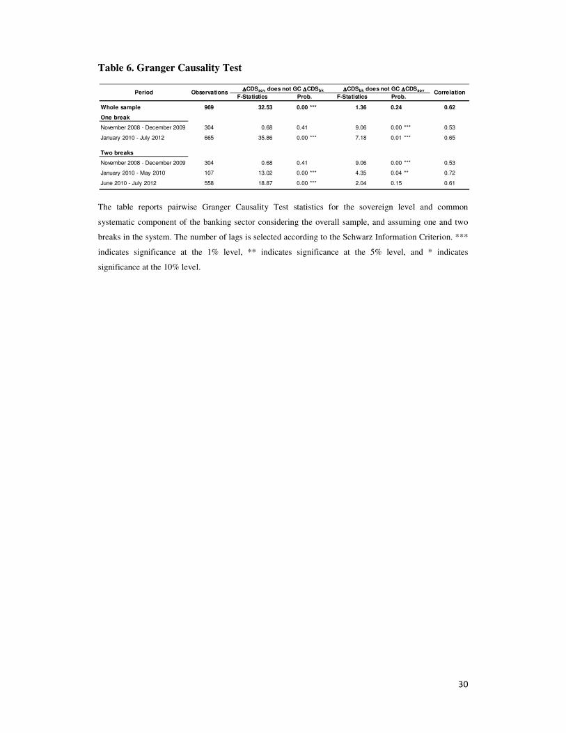
Taken together, all conducted tests show strong evidence in favor of the

presence of the structural changes in the system. Thus, in reference to the previous

analysis and several patterns revealed, we divide data into three sub-periods: November

2008 to December 2009, January 2010 to May 2010 and June 2010 to July 2012, and

conduct Granger Causality tests for the three periods separately. Results are reported in

Table 6. The first sub-period (November 2008 to December 2009) is characterized with

the one-way influence of the banking sector on the sovereign CDS spreads. The second-

sub period (January 2010 – May 2010) is characterized with a two-way feedback mean

transmission mechanism between banking sector and the government. This interim

period coincides with the consolidation of the Spanish banking system and major

restructuring of the saving banks; the European Commission approval of the Spanish

recapitalization scheme for credit institutions that sharply increased investors’

expectation of government support to distressed banks; and substantial increase in the

CDS spread levels across Eurozone countries following the announcement of the newly

appointed Greek government of much larger than expected budget deficit (from

13

originally stated 6% to 12.7% of GDP) in October 2009. This event raised uncertainty

about the quality of banks’ assets and led to reassessment, from part of investors, of the

sovereigns’ perceived creditworthiness across Eurozone. As a feedback effect increased

sovereign credit risk directly negatively affected the quality of the bank’s assets through

their holdings of sovereign debt, and the value of collateral that can be used for funding.

Moreover, Spain’s debt rating was downgraded (from AAA to AA+ on May 28 by

Fitch, and from AA+ to AA by S&P in April ), leading to a cascade of downgrades of

Spanish domestic banks. The third-sub period (June 2010 to July 2012) is characterized

with a clear one-way influence from sovereign CDS spreads to banking sector CDS

spreads. The third sub-period starts with the pronounced break in the mean transmission

between sovereign and banking sector CDS spreads that occurred in the mid-May 2010

which coincides with the government public announcement of the severe austerity

measures on the May 12, 2010. This event severely raised investors concerns about

Spanish government deficit, negatively affecting investors’ perception about the value

of implicit and explicit government guarantees to banks. Moreover, it followed the first

EU-IMF bailout of Greece at the May 2, 2010 when Greece received a 110 billion

rescue package conditional on a series of severe austerity measures. These results of the

sub-period Granger causality tests are substantially different from the results for the

complete data set suggesting that without controlling for relevant structural breaks

wrong conclusions about the transmission mechanism could be made.


In light of the previous findings we augment each equation of the baseline VAR

system with the interaction break dummy variables, allowing interactions with intercept

and slope coefficients (i.e. lags of the endogenous variables) preserving in this way the

14

symmetry in the VAR system. The mean return generating process is defined as

follows:

�� = � + Γ�� + 2��#3� + D�� $ + 2��#3� + D�� $ + ��, (3)

where �� is a 2 × 1 vector of daily CDS spread log-changes at time t of sovereign

(��,� = ��,�) and banking sector (��,� = ��,�); 2�� is a dummy variable that takes the

value 1 if the observation belongs to the first sub-period (November 2008 – December

2009) and 0 otherwise and 2�� is transition period dummy variable that takes the value 1

if the observation belongs to the second sub-period (January 2010 – May 2010) and 0

otherwise. In this way we consider a VAR model with the three structural regime shifts

that reflect the change in the dynamics of the mean transmission. The own market

segment mean spillovers and cross market segment mean spillovers are measured by the

estimates of the matrix Γ, D� and D�. The diagonal elements of the corresponding

matrix measure the effect of the own lagged returns, and the off-diagonal elements the

effect of the cross-market lagged returns. Thus, the off-diagonal elements detect the

return spillover.

3. Volatility transmission

The traditional VAR model applied in recent papers is based on the assumption

of homoscedasticity of residuals. Given that the time series of CDS returns resembles a

GARCH process we estimate a bivariate VAR-BEKK-GARCH model proposed by

Engle and Kroner (1995). We consider the full BEKK representation of Baba, Engle,

Kraft, and Kroner (1990) that allows for the time-varying variance-covariance matrix

and, by construction, guarantees that the estimated conditional covariance matrix is

positive definite. Specifically, in order to capture conditional heteroskedasticity and

estimate volatility transmission throughout the financial system we estimate the regime-

15

switching VAR(1)-GARCH(1,1) model within the BEKK framework of the following

form:

8��|Ω; �~=#0, ?�$ (4a)

where

?� = @A@ + BA�� A B + CA?� �C (4b)

?� = DE��,� E��,�E��,� E��,�F; @ = DG�� G��0 G��F; B = DH�� H��H�� H��F ; C = JK�� K��

K�� K��L

�� = "��,� ��,�%A

The �� is a 2 × 1 vector of residuals, i.e. vector of innovations for each market segment

at time t, with its corresponding conditional covariance matrix, ?�. The market

information available at time t-1 is represented by the information set Ω; �.

Equation (4) defines the variance generating process. The ?� is the 2 × 2

conditional variance-covariance matrix of residuals, that, in the bivariate case of the

model, requires 11 parameters to be estimated. The matrix C is an upper triangular

matrix containing the constants for the variance equation. The ARCH coefficients are

derived from the A matrix and the GARCH coefficients are derived from B matrix. We

choose the GARCH(1,1) as this specification is showed to be sufficient to provide

parsimonious results. The model is estimated using the maximum likelihood estimation

procedure. The log-likelihood function is given by:

M = N M�#O$ =P

��N -−()#2R$ − 1

2 ()|?�| − 12 ��A?� ��.

P

��

The BHHH (Berndt, Hall, Hall, and Hausman (1974)) algorithm is used to maximize

the log-likelihood function. The starting values for the constants in the conditional

variance-covariance equations are obtained from univariate GARCH. The convergence

criterion is 1e-5.

16

3.1. Main Results

The results from estimating bivariate VAR-BEKK-GARCH model described

with equations (3) and (4) are provided in Table 7.6 The mean spillovers are measured

with the parameters of Γ matrix. Specifically, the parameters of Γ matrix measure the

effects of innovation in one segment of the market to its own lagged return (diagonal

elements) and that of the other segment (off-diagonal elements). For example, ��,

measures the effect that the a change in banking sector CDS return has on the sovereign

sector CDS return in one day time. Given that we consider a regime-switching model

these coefficients have to be interpreted together with the elements provided in matrix

D� and D�. Considering the common banking sector component, as well as individual

banks we can observe the same pattern: the mean transmission from the banking sector

to the government was the strongest in the first period, decreased in the second, and

completely turned around in the third sub-period in which we observe a highly

pronounced mean transmission from government to the banking sector. Specifically, ��

coefficient is positive and statistically significant at 1% level not only for the common

banking sector component but also for all of the banks considered on an individual

basis.


The ARCH parameters are represented by matrix A whereas the coefficients of

matrix B measure the influence of lagged conditional variances and covariances on the

conditional variance today. These coefficients measure the volatility clustering and the

larger the coefficient the longer is the effect of shocks.

6 The covariance stationarity in the BEKK model is ensured if eigenvalues of #B⨂B$ + #C⨂C$,

are less than one in modulus. The biggest of eignevalues is around 0.98 in modules which means that time

varying volatility is highly persistent. We check the adequacy of the VAR-BEKK-GARCH specification

using the Ljung-Box Q-statistic and Lagrange Multiplier (LM). We report Ljung-Box statistics for

standardized squared residuals up to lag 12 and 24. The results show no serial dependence in the

standardized squared residuals which indicates that the model is appropriate and that is able to capture the

dynamics of the conditional volatility well.

17

The diagonal elements of A and B matrices measure the effect of the own past

shocks (HTT) and past volatility (KTT). The a11 measures the dependence of conditional

sovereign CDS return volatility on its own lagged past shocks, and a22 the dependence

of conditional banking sector CDS return volatility on its own lagged past shocks. The

a11 and a22 coefficients are statistically significant at 1% level in all of the cases,

indicating that there were strong ARCH effects. The b11 measures the dependence of

conditional sovereign CDS return volatility on its own lagged volatility, and b22 the

dependence of conditional banking sector CDS return volatility on its own lagged

volatility. The b11 and b22 coefficients are statistically significant at 1% level in all of the

cases, indicating that there were strong GARCH effects.

We are here particularly interested in the off-diagonal elements as these will

reveal the volatility spillovers across the market segments considered. The coefficient

HT measures the spillover of the squared values of shocks in the previous period from

the ith

to the current volatility of jth

market. The a21 measures the dependence of

conditional sovereign CDS return volatility on the lagged shocks of bank CDS returns.

The a21 coefficient is statistically significant at 1% level for the banking sector credit

risk component, and individually for Banco Santander, BBVA, La Caixa and Bankinter.

The opposite effect, the dependence of conditional banking sector CDS return volatility

on the lagged shocks of sovereign CDS returns is measured with the a12 coefficient.

This coefficient is statistically significant at least at 5% level in the case of BBVA,

Banco Popular, Banco Sabadell and Bankinter. Nevertheless, the common banking

sector component is not statistically significant.

On the other hand, KT measures the spillover of the conditional volatility of the

ith

market in the previous period to the jth

market in the current period. The b21 measures

the dependence of conditional sovereign CDS return volatility on the lagged volatility

18

of bank CDS returns. The b21 coefficient is statistically significant at 1% for the

common banking sector component, Banco Santander, BBVA and La Caixa. The b12

measures the dependence of conditional banking sector CDS return volatility on the

lagged volatility of sovereign CDS returns. The common banking sector component as

well as the volatility of CDS returns of BBVA, Banco Pastor, Banco Popular and

Bankinter are affected by lagged volatility of sovereign CDS returns.

Figure 6 presents conditional variances and covariances for sovereign CDS

returns and first principal component of the banking sector CDS returns. The peak in

conditional variances and covariances refers to 11th

of May 2010, which coincides with

the abrupt break detected in the mean transmission. The time-varying conditional

correlations between sovereign returns and common factor in banks’ returns, presented

in Figure 7 are positive throughout the sample period, ranging from minimum of 0.21

and maximum of 0.95, with the mean of 0.56. The positive correlations for the overall

sample period considered suggest that the two variables are interconnected.



In conclusion, although there is an evidence of the two-way volatility

transmission between sovereign and banking sector CDS returns the results of the

variance equation show that volatility transmission from banking sector to sovereign

sector is particularly evident in the case of the 3 largest Spanish banks: Banco

Santander, BBVA and La Caixa, whereas the opposite doesn’t hold. Namely, the

volatility transmission from sovereign to banking sector seems to be less pronounced

for these financial institutions and, specifically, we do not find any evidence of the

volatility transmission from sovereign level to CDS spread returns of Banco Santander

and La Caixa.

19

3.2. Structural changes in the volatility transmission

In order to detect eventual changes in the volatility transmission it is possible to

apply Granger Causality test directly on time-varying variances in a VAR framework of

the following form:

E��,� = �� + ∑ ��,�� E��,� � + ∑ ��,�

�� E��,� � + ��,� , (5)

E��,� = �� + ∑ ��,�� E��,� � + ∑ ��,�

�� E��,� � + ��,� . (6)

where E��,� is the time-varying sovereign CDS return volatility and E��,� is the time-

varying banking sector CDS return volatility , ε1 and ε2 are i.i.d. error terms, and p is the

number of lags determined according to the Schwarz Information Criterion. The optimal

number of lags is 3. In line with previous analysis we test for the structural breaks in the

VAR system and find a significant break point that again coincides with the May 12,

2010. Once the overall sample is divided in two subsamples, and the structural break

point tests reapplied on the two subsamples, additional break point can be detected only

in the first sub-period, and coincides with January 28, 2010. These results, presented in

Table 8, are quite in line with the breaks detected in the mean transmission and

independent of whether sovereign and banking sector volatility is calculated before or

after accounting the changes in the mean transmission. Finally, the results of the

pairwise Granger Causality tests are presented in Table 9.



4. Conclusions

The mechanism of shock transmissions between sovereign and banking sector

default risk has important implications for financial stability, but is not well understood.

This paper shed light upon this issue by empirically investigating the mean and

20

volatility transmission channel through which increased sovereign credit risk can spill

over to the banking sector by increasing the financing costs of banks (and vice versa),

using the sample of systematically important banks in Spain during the period 2008-

2012. We contribute to the existing literature in two ways. First, unlike previous studies,

we endogenously search for potential structural breaks in the mean and volatility

transmission mechanism. Our main results show that there is an evident change in the

mean return transmission over the period examined: from a pronounced one-way bank

to sovereign transmission at the beginning of the period, to a pronounced one-way

sovereign to bank transmission since mid-May 2010. Endogenously identified break

dates coincide with important events for the Spanish financial system that severely

affected investors’ perception of the government implicit and explicit support to

distressed banks. Second, we account not only for the conditional mean but also for the

conditional variance using the VAR-BEKK-GARCH framework. We find evidence of

two-way volatility transmission between sovereign and banking sector CDS returns,

with strong volatility transmission from the three largest banks in Spain to the sovereign

level. Moreover, we provide preliminary evidence of the changes in the volatility

transmission from two-way transmission to one-way sovereign to bank transmission

since mid-May 2010.

21

References

Acharya, V.V., Drechsler, I., and Schnabl, P., 2011, “A Pyrrhic Victory? - Bank Bailouts and

Sovereign Credit Risk”, NBER Working Paper No. 17136;

Alter, A., and Schüler Y.S., 2012, “Credit spread interdependencies of European states and

Banks during the financial crisis”, Journal of Banking and Finance, 36, 3444-3468;

Andrews, D.W.K., 1993, “Tests for parameter instability and structural change with

unknown change point”, Econometrica, 61, 821-856;

Andrews, D.W.K., and Ploberger, W., 1994, “Optimal tests when a nuisance parameter is

present only under the alternative”, Econometrica, 62, 1383-1414;

Attinasi, M.G., Checherita, C., and Nickel, C., 2009, “What explains the surge in Euro Area

sovereign spreads during the financial crisis of 2007-09?”, EBC Working paper 1131;

Baba, Y., R.F. Engle, D. Kraft, and K. Kroner, 1990, Multivariate simultaneous generalized

ARCH, unpublished manuscript, University of California, San Diego;

Bai, J., 1997, “Estimating multiple breaks one at a time”, Economic Theory, 13(3), 315-352;

Bai, J., Lumsadine, R.L., and Stock, J.H., 1998, “Testing for and dating common breaks in

multivariate time series”, Review of Economic Studies, 65, 395-432;

Bai, J., and Perron, P., 1998, “Estimating and testing linear models with multiple structural

changes”, Econometrica, 66, 47-78;

Bai, J., and Perron, P., 2003, “Computation and analysis of multiple structural change

models”, Journal of Applied Econometrics, 18, 1-22;

Candelon, B., and Lütkepohl, H., 2001, “On the reliability of Chow-type tests for parameter

constancy in multivariate dynamic models”, Economics Letters, 73, 155-160;

Dieckmann, S., and Plank, T., 2011, “Default Risk of Advanced Economies: An Empirical

Analysis of Credit Default Swaps during the Financial Crisis”, Working paper;

Engle, R.F., and Kroner, K.F., 1995, “Multivariate Simultaneous Generalized ARCH”,

Econometric Theory, 11(5), 122-150;

Gerlach, S., Schulz, A., and Wolff, G., 2010, “Banking and Sovereign Risk in the Euro

Area”, Deutsche Bundesbank Discussion Paper No. 09;

22

Hansen, B., 1997, “Approximate asymptotic p values for structural change tests”, Journal of

Business and Economic Statistics, 1, 60-67;

Hansen,B., 2000, “Testing for structural change in conditional models”, Journal of

Econometrics, 97(1), 93-115;

Kalbaska, A., and Gatkowski, M., 2012, “Eurozone sovereign contagion: Evidence from the

CDS market (2005-2010)”, Journal of Economic Behavior & Organization (forthcoming);

Kallestrup, R., Lando, D., and Murgoci, A., 2012, “Financial sector linkages and the

dynamics of bank and sovereign credit spreads”, Working paper;

Lütkepohl, H, and M. Kratzig, 2004, “Applied Time Series Econometrics”, Cambridge

University Press;

Quandt, R., 1960, “Tests of the hypothesis that a linear regression system obeys two separate

regimes”, Journal of the American Statistical Association, 55, 324-330;

23

Figure 1. Daily sovereign and banking CDS returns

Figure 2. Bootstrapped p-values from the sample-split test

0 100 200 300 400 500 600 700 800 900 1000-15

-10

-5

0

5

10

Sovereign CDS returns

0 100 200 300 400 500 600 700 800 900 1000-0.5

-0.4

-0.3

-0.2

-0.1

0

0.1

0.2

0.3

Banking sector CDS returns

100 200 300 400 500 600 700 800 9000

0.1

0.2

0.3

0.4

0.5

0.6

0.7

0.8

0.9

1

Sample-split test: bootstrapped p-values

Q 2 (12) 187,35

p -val 0,00

Q 2 (24) 206,86

p -val 0,00

LM2 (12) 136,04

p -val 0,00

LM2 (24) 140,96

p -val 0,00

Q 2 (12) 278,76

p -val 0,00

Q 2 (24) 329,98

p -val 0,00

LM2 (12) 197,25

p -val 0,00

LM2 (24) 202,47

p -val 0,00

24

Figure 3. Bootstrapped p-values before and after January 6th 2010

Figure 4. Recursive Granger causality tests (p-values) – banking sector component

The graph represents p-values of recursive Granger Causality tests estimated by adding consecutively one

observation to the sample.

50 100 150 200 2500

0.1

0.2

0.3

0.4

0.5

0.6

0.7

0.8

0.9

1

Sample-split test (before January 6, 2010): bootstrapped p-values

400 500 600 700 800 9000

0.1

0.2

0.3

0.4

0.5

0.6

0.7

0.8

0.9

1

Sample-split test (after January 6, 2010): bootstrapped p-values

100 200 300 400 500 600 700 800 9000

0.1

0.2

0.3

0.4

0.5

0.6

0.7

0.8

0.9

1

SOV dngc BK (p-val)

BK dngc SOV (p-val)

5% level

10% level

25

Figure 6. Conditional variances for sovereign and banks CDS returns

Figure 7. Conditional correlations between sovereign and banks CDS returns

0 100 200 300 400 500 600 700 800 900 10000.2

0.3

0.4

0.5

0.6

0.7

0.8

0.9

1

Conditional correlations between sovereign and banking sector CDS returns

0 100 200 300 400 500 600 700 800 900 10000

10

20

30

40

50

60

Conditional variance of banking sector CDS returns

0 100 200 300 400 500 600 700 800 900 10000

0.005

0.01

0.015

0.02

0.025

0.03

Conditional variance of sovereign CDS returns

26

Table 1. Summary statistics of sovereign and banking sector CDS spreads

This table provides main summary statistics for Spanish sovereign CDS spreads and CDS spreads of

seven major financial institutions in Spain. ADF unit root tests are performed for three possible

alternatives: without constant and trend in the series, with constant and without trend, and with constant

and trend. Reported ADF test statistics correspond to the model with the lowest Schwartz Information

Criterion, where the number of lags is determined according to the Akaike Information Criterion. Panel A

depicts main descriptive statistics in CDS spread levels and Panel B main descriptive statistics of CDS

spread returns expressed in %. CDS returns are calculated as log differences.

Table 2. Principal component analysis

This table provides results from principal component analysis conducted on CDS spread levels and CDS

spread changes.

t -stat p -val

Spain 193.31 472.62 47.00 106.82 0.63 2.41 78.32 0.00 -2.90 0.16

Banco Santander 211.57 487.76 63.00 112.10 0.62 2.53 72.13 0.00 -3.21 0.08

BBVA 205.60 487.59 66.16 109.65 0.69 2.46 89.51 0.00 0.67 0.86

La Caixa 238.30 446.42 82.75 81.64 -0.19 2.45 18.09 0.00 0.02 0.69

Banco Pastor 510.92 1387.23 165.00 253.43 1.23 4.27 311.45 0.00 -0.01 0.68

Banco Popular 387.96 872.33 133.00 221.03 0.87 2.44 135.72 0.00 0.47 0.82

Banco Sabadell 388.15 837.91 133.71 204.69 0.88 2.49 135.31 0.00 0.46 0.81

Bankinter 364.06 820.09 137.50 184.95 0.93 2.69 144.63 0.00 0.10 0.71

t -stat p -val

Spain 0.1689 28.26 -41.75 5.45 -0.35 8.63 1,298.74 0.00 -18.22 0.00

Banco Santander 0.1533 20.97 -40.06 4.91 -0.62 9.87 1,966.51 0.00 -17.64 0.00

BBVA 0.1914 17.04 -37.33 4.58 -0.77 10.88 2,600.43 0.00 -16.73 0.00

La Caixa 0.0481 23.61 -27.50 3.80 -0.09 14.14 5,008.51 0.00 -29.25 0.00

Banco Pastor 0.0922 39.33 -43.53 4.27 -1.05 34.19 39,454.27 0.00 -32.17 0.00

Banco Popular 0.1497 18.64 -21.15 3.18 -0.43 14.69 5,546.80 0.00 -26.00 0.00

Banco Sabadell 0.1316 15.83 -17.22 2.97 -0.04 10.22 2,105.86 0.00 -15.09 0.00

Bankinter 0.1317 22.31 -32.61 3.61 -0.24 19.61 11,148.33 0.00 -16.66 0.00

Panel A

Panel B

ADF test

ADF testSD Skew p -value

Kurt

Kurt

Jarq-B

Jarq-BEntity Min

p -valueSkewSD

Mean Max

MinEntity Mean Max

loadings corr(bank, FC1) loadings corr(bank, FC1)

Banco Santander 0.387 0.94 0.422 0.79

BBVA 0.383 0.95 0.432 0.81

La Caixa 0.284 0.70 0.388 0.73

Banco Pastor 0.379 0.93 0.234 0.44

Banco Popular 0.402 0.99 0.364 0.68

Banco Sabadell 0.401 0.98 0.426 0.80

Bankinter 0.395 0.97 0.339 0.64

First component 85.9% 50.1%

BankCDS levles CDS changes

27

Table 3. Granger Causality Test

The table reports pairwise Granger Causality Test statistics for the common systematic component of the

banking sector and the individual banks when overall sample period is considered (November 2008 – July

2012). The number of lags is selected according to the Schwarz Information Criterion. *** indicates

significance at the 1% level, ** indicates significance at the 5% level, and * indicates significance at the

10% level.

F-Statistics F-Statistics

First component 32.53 0.00 *** 1.36 0.24 0.62

Banco Santander 24.53 0.00 *** 1.83 0.18 0.66

BBVA 38.54 0.00 *** 1.49 0.22 0.65

La Caixa 46.99 0.00 *** 1.14 0.29 0.44

Banco Pastor 30.69 0.00 *** 2.00 0.16 0.20

Banco Popular 24.33 0.00 *** 0.71 0.40 0.33

Banco Sabadell 43.89 0.00 *** 4.25 0.04 ** 0.41

Bankinter 35.82 0.00 *** 5.20 0.02 ** 0.28

CorrelationBank∆∆∆∆CDSsov does not GC ∆∆∆∆CDSbk ∆∆∆∆CDSbk does not GC ∆∆∆∆CDSsov

Prob. Prob.

28

Table 4. Tests for structural breaks – individual equations

This table reports �� and &'�� break-point tests. Panel A reports results for individual CDS return series, and Panel B results for individual equations of the benchmark

VAR described in (1) and (2). The p-values are calculated as: a) asymptotic p-values using the approximation of Hansen (1997) – Approximate p-value, b) fixed-regressor

bootstrap values developed in Hansen (2000) – Bootstrap p-value(1)

, c) replacement bootstrap values developed in Candelon and Lütkepohl (2001) – Bootstrap p-value(2)

, and

d) robust “wild” bootstrap values – Bootstrap p-value(3). The number of bootstrap replications is set to 1,000.

Test

statistic

Approximate

p-value

Bootstrap

p-value(1)

Bootstrap

p-value(2)

Bootstrap

p-value(3)

Test

statistic

Approximate

p-value

Bootstrap

p-value(1)

Bootstrap

p-value(2)

Bootstrap

p-value(3)

Second series: yBK

SupF 1.88 0.815 0.816 0.807 0.781 SupF 4.72 0.278 0.280 0.290 0.232

ExpF 0.15 0.898 0.871 0.882 0.872 ExpF 0.64 0.344 0.346 0.350 0.3340.887 0.403

Test

statistic

Approximate

p-value

Bootstrap

p-value(1)

Bootstrap

p-value(2)

Bootstrap

p-value(3)

Test

statistic

Approximate

p-value

Bootstrap

p-value(1)

Bootstrap

p-value(2)

Bootstrap

p-value(3)

VAR equation (1): ySOV VAR equation (2): yBK

H0: Stability of all coefficients H0: Stability of all coefficients

Ha: There is a structural break Ha: There is a structural break

SupF 15.37 0.027 0.032 0.035 0.050 SupF 13.21 0.065 0.054 0.067 0.101

ExpF 5.52 0.017 0.017 0.020 0.031 ExpF 3.57 0.095 0.081 0.078 0.142

H0: Stability of the constant coefficient H0: Stability of the constant coefficient

SupF 1.40 0.930 0.918 0.918 0.916 SupF 3.27 0.501 0.494 0.511 0.490

ExpF 0.11 1.000 0.936 0.938 0.942 ExpF 0.33 0.605 0.599 0.610 0.603

H0: Stability of the slope coefficients H0: Stability of the slope coefficients

SupF 14.72 0.013 0.011 0.014 0.030 SupF 12.35 0.036 0.030 0.037 0.051

ExpF 5.38 0.006 0.004 0.007 0.017 ExpF 3.01 0.061 0.064 0.057 0.070

H0: Stability of the variance H0: Stability of the variance

SupF 11.83 0.011 0.008 0.015 0.010 SupF 5.14 0.233 0.238 0.187 0.199

ExpF 2.96 0.016 0.017 0.015 0.012 ExpF 1.31 0.127 0.138 0.110 0.128

GARCH filtered residuals GARCH filtered residuals

SupF 4.45 0.312 0.333 0.294 0.269 SupF 2.50 0.664 0.665 0.656 0.626

ExpF 0.52 0.422 0.443 0.438 0.423 ExpF 0.29 0.658 0.656 0.667 0.676

First series: ySOV

Panel A

Panel B

29

Table 5. Tests for structural break in VAR system

This table reports �� and &'�� break-point tests in VAR system described in (1) and (2). Panel A reports results for the overall sample period, Panel B results for the first

sub-period, from November 2008 to December 2009, and Panel C results for the second sub-period, from January 2010 to July 2012. The p-values are calculated as: a)

asymptotic p-values using the approximation of Hansen (1997) – Approximate p-value, b) fixed-regressor bootstrap values developed in Hansen (2000) – Bootstrap p-value(1)

,

c) replacement bootstrap values developed in Candelon and Lütkepohl (2001) – Bootstrap p-value(2)

, and d) robust “wild” bootstrap values – Bootstrap p-value(3)

. The number

of bootstrap replications is set to 1,000.

Test

statistic

Approximate

p-value

Bootstrap

p-value(1)

Bootstrap

p-value(2)

Bootstrap

p-value(3)

Test

statistic

Approximate

p-value

Bootstrap

p-value(1)

Bootstrap

p-value(2)

Bootstrap

p-value(3)

Test

statistic

Approximate

p-value

Bootstrap

p-value(1)

Bootstrap

p-value(2)

Bootstrap

p-value(3)

VAR system VAR system VAR system

H0: Stability of all coefficients H0: Stability of all coefficients H0: Stability of all coefficients

Ha: There is a structural break Ha: There is a structural break Ha: There is a structural break

SupF 20.32 0.045 0.043 0.040 0.090 SupF 10.99 0.598 0.592 0.584 0.574 SupF 19.78 0.054 0.055 0.052 0.096

ExpF 7.68 0.028 0.025 0.035 0.065 ExpF 3.33 0.570 0.574 0.596 0.591 ExpF 5.72 0.127 0.134 0.120 0.206

H0: Stability of the constant coefficient H0: Stability of the constant coefficient H0: Stability of the constant coefficient

SupF 3.95 0.735 0.736 0.734 0.727 SupF 8.97 0.142 0.152 0.145 0.129 SupF 9.90 0.099 0.089 0.113 0.099

ExpF 0.39 0.939 0.925 0.917 0.937 ExpF 2.51 0.104 0.118 0.111 0.110 ExpF 1.52 0.303 0.301 0.312 0.305

H0: Stability of the slope coefficients H0: Stability of the slope coefficients H0: Stability of the slope coefficients

SupF 17.83 0.027 0.030 0.022 0.070 SupF 3.95 0.985 0.982 0.972 0.956 SupF 15.99 0.055 0.050 0.064 0.093

ExpF 6.89 0.010 0.012 0.012 0.043 ExpF 0.83 0.989 0.984 0.980 0.966 ExpF 3.60 0.192 0.214 0.197 0.256

Panel C:

Second sub-period

Panel B:

First sub-period

Panel A:

Whole sample

30


The table reports pairwise Granger Causality Test statistics for the sovereign level and common

systematic component of the banking sector considering the overall sample, and assuming one and two

breaks in the system. The number of lags is selected according to the Schwarz Information Criterion. ***

indicates significance at the 1% level, ** indicates significance at the 5% level, and * indicates

significance at the 10% level.


Whole sample 969 32.53 0.00 *** 1.36 0.24 0.62

One break

November 2008 - December 2009 304 0.68 0.41 9.06 0.00 *** 0.53

January 2010 - July 2012 665 35.86 0.00 *** 7.18 0.01 *** 0.65

Two breaks

November 2008 - December 2009 304 0.68 0.41 9.06 0.00 *** 0.53

January 2010 - May 2010 107 13.02 0.00 *** 4.35 0.04 ** 0.72

June 2010 - July 2012 558 18.87 0.00 *** 2.04 0.15 0.61

CorrelationProb. Prob.

Period Observations∆∆∆∆CDSsov does not GC ∆∆∆∆CDSbk ∆∆∆∆CDSbk does not GC ∆∆∆∆CDSsov

31

Table 7. The regime-switching VAR-BEKK-GARCH(1,1)

This table presents the regression estimation results allowing for three shifts. d1 is a dummy variable that

takes the value 1 if the observation belongs to the first sub-period (November 2008 – December 2009)

and 0 otherwise and d2 is a dummy variable that takes the value 1 if the observation belongs to the second

sub-period (January 2010 – May 2010) and 0 otherwise. Constant terms are not are not reported to save

space. *** indicates significance at the 1% level, ** indicates significance at the 5% level, and * indicates


Parameter

γ11 0.218 *** 0.122 ** 0.182 *** 0.193 *** 0.193 *** 0.190 *** 0.188 *** 0.203 ***

γ12 -0.002 0.088 -0.018 -0.061 -0.139 ** -0.088 -0.065 -0.143 **

γ21 7.829 *** 0.194 *** 0.296 *** 0.172 *** 0.139 *** 0.056 ** 0.104 *** 0.137 ***

γ22 0.143 *** 0.060 -0.051 -0.035 -0.023 0.177 *** 0.107 ** -0.079 *

d111

-0.179 * -0.093 -0.170 -0.048 -0.035 -0.051 -0.039 -0.048

d121

0.009 *** 0.122 0.254 ** 0.159 0.156 * 0.196 0.163 0.244 *

d211

-6.325 * -0.118 -0.246 *** -0.113 * -0.029 0.021 -0.005 -0.086

d221

0.155 0.091 0.250 *** -0.087 -0.086 -0.064 -0.086 0.050

d112

0.119 0.179 * 0.036 0.093 0.021 0.029 0.139 * 0.026

d122

-0.005 * -0.300 ** -0.064 -0.251 * -0.103 -0.172 -0.508 *** -0.113

d212

5.165 0.149 -0.049 0.053 0.011 0.108 ** 0.062 0.049

d222

-0.170 * -0.337 *** -0.022 -0.004 -0.045 -0.162 * -0.047 -0.081

c11 0.006 * 0.009 *** 0.007 *** 0.007 *** 0.016 *** 0.006 *** 0.007 *** 0.004

c12 0.398 ** 0.014 *** 0.006 * 0.006 0.005 *** -0.001 0.002 -0.028

c22 0.509 *** 0.004 *** 0.012 *** 0.013 *** 0.008 *** 0.007 *** 0.006 *** 0.000

a11 0.179 *** 0.186 *** 0.160 *** 0.210 *** 0.342 *** 0.235 *** 0.235 *** 0.202 ***

a12 0.805 0.010 -0.061 *** 0.023 0.010 -0.032 ** 0.031 ** -0.252 ***

a21 0.005 *** 0.158 *** 0.214 *** 0.140 *** 0.018 0.063 0.039 0.221 ***

a22 0.468 *** 0.411 *** 0.446 *** 0.564 *** 0.232 *** 0.223 *** 0.287 *** 0.400 ***

b11 0.996 *** 0.989 *** 0.981 *** 0.975 *** 0.888 *** 0.966 *** 0.965 *** 0.984 ***

b12 2.044 ** 0.010 0.040 * 0.019 -0.034 *** 0.017 *** -0.002 0.215 ***

b21 -0.002 *** -0.089 *** -0.068 *** -0.067 *** 0.009 -0.012 -0.015 -0.266 *

b22 0.766 *** 0.850 *** 0.832 *** 0.752 *** 0.956 *** 0.944 *** 0.928 *** 0.322 ******

Log likelihood -106.607 3,450.88 3,515.23 3,548.58 3,282.82 3,598.80 3,741.41 3,448.33

AIC 0.25 -7.11 -7.24 -7.31 -6.76 -7.42 -7.71 -7.11

SC 0.31 -7.04 -7.18 -7.25 -6.70 -7.35 -7.65 -7.05

LR(χ2) 387.27 475.65 452.50 137.62 57.65 97.83 122.24 76.16

LR(p -val) 0.00 0.00 0.00 0.00 0.00 0.00 0.00 0.00

Q2(12) 9.61 10.80 7.08 4.47 14.46 5.01 4.61 3.26

p -val 0.65 0.55 0.85 0.97 0.27 0.96 0.97 0.99

Q2(24) 31.24 15.61 15.60 9.53 21.39 17.87 20.80 8.92

p -val 0.15 0.90 0.90 1.00 0.62 0.81 0.65 1.00

LM2(12) 8.92 10.77 6.59 4.76 13.34 5.82 5.28 3.20

p -val 0.71 0.55 0.88 0.97 0.34 0.93 0.95 0.99

LM2(24) 31.09 14.88 15.29 10.68 20.91 22.64 22.02 8.65

p -val 0.15 0.92 0.91 0.99 0.64 0.54 0.58 1.00

BankinterBBVAFirst

component

Banco

SantanderLa Caixa

Banco

Pastor

Banco

Popular

Banco

Sabadell

32

Table 8. Tests for structural break in volatility transmission

This table reports �� and &'�� break-point tests in VAR system described in (5) and (6). Panel A reports results for the overall sample period, Panel B results for the first

sub-period, from November 2008 to May 2010, and Panel C results for the second sub-period, from June 2010 to July 2012. The p-values are calculated as: a) asymptotic p-

values using the approximation of Hansen (1997) – Approximate p-value, b) fixed-regressor bootstrap values developed in Hansen (2000) – Bootstrap p-value(1)

, c)

replacement bootstrap values developed in Candelon and Lütkepohl (2001) – Bootstrap p-value(2), and d) robust “wild” bootstrap values – Bootstrap p-value

(3). The number of

bootstrap replications is set to 1,000.

Test

statistic

Approximate

p-value

Bootstrap

p-value(1)

Bootstrap

p-value(2)

Bootstrap

p-value(3)

Test

statistic

Approximate

p-value

Bootstrap

p-value(1)

Bootstrap

p-value(2)

Bootstrap

p-value(3)

Test

statistic

Approximate

p-value

Bootstrap

p-value(1)

Bootstrap

p-value(2)

Bootstrap

p-value(3)

VAR system - before accounting for changes in the mean



SupF 98.93 0.000 0.000 0.021 0.020 SupF 45.19 0.001 0.002 0.121 0.067 SupF 27.58 0.211 0.243 0.476 0.767

Exp 42.95 0.000 0.000 0.021 0.021 Exp 18.66 0.001 0.004 0.102 0.067 Exp 10.92 0.175 0.199 0.393 0.736

Ave 30.16 0.000 0.000 0.017 0.084 Ave 25.88 0.004 0.008 0.025 0.053 Ave 16.25 0.236 0.246 0.320 0.631

VAR system - after accounting for changes in the mean



SupF 108.41 0.000 0.000 0.006 0.005 SupF 41.68 0.004 0.006 0.160 0.075 SupF 27.24 0.227 0.232 0.520 0.761

Exp 47.69 0.000 0.000 0.007 0.006 Exp 16.76 0.005 0.008 0.157 0.080 Exp 10.76 0.190 0.212 0.442 0.731

Ave 31.36 0.000 0.000 0.011 0.067 Ave 23.45 0.013 0.020 0.049 0.068 Ave 16.08 0.250 0.242 0.330 0.634

Panel A:

Whole sample

Panel B:

First sub-period

Panel C:

Second sub-period

33


The table reports pairwise Granger Causality Test statistics for the variance of the sovereign CDS returns

and variance of the banking sector CDS returns considering the overall sample, and assuming one and

two breaks in the system. The number of lags is selected according to the Schwarz Information Criterion.

*** indicates significance at the 1% level, ** indicates significance at the 5% level, and * indicates



Whole sample 969 6.12 0.00 *** 8.26 0.00 ***

One break

November 2008 -May 2010 411 5.19 0.00 *** 13.85 0.00 ***

June 2010 - July 2012 558 4.09 0.04 ** 2.05 0.15

Two breaks

November 2008 - January 2009 321 1.13 0.34 3.95 0.01 ***

February 2010 - May 2010 90 0.64 0.59 1.65 0.18

June 2010 - July 2012 558 4.09 0.04 ** 2.05 0.15

Period Observationsσσσσsov does not GC σσσσbk σσσσbk does not GC σσσσsov

Prob. Prob.

structural changes in the transmission mechanism between banking and ... annual...

Documents