This content has been downloaded from IOPscience. Please scroll down to see the full text.

Download details:

IP Address: 152.1.52.166

This content was downloaded on 04/12/2015 at 17:06

Please note that terms and conditions apply.

Strongly correlated quantum fluids: ultracold quantum gases, quantum chromodynamic

plasmas and holographic duality

View the table of contents for this issue, or go to the journal homepage for more

2012 New J. Phys. 14 115009

(http://iopscience.iop.org/1367-2630/14/11/115009)

Home Search Collections Journals About Contact us My IOPscience

Strongly correlated quantum fluids: ultracoldquantum gases, quantum chromodynamic plasmasand holographic duality

Allan Adams1, Lincoln D Carr2,3,6, Thomas Schafer4,Peter Steinberg5 and John E Thomas4

1 Center for Theoretical Physics, MIT, Cambridge, MA 02139, USA2 Physics Institute, University of Heidelberg, D-69120 Heidelberg, Germany3 Department of Physics, Colorado School of Mines, Golden, CO 80401, USA4 Department of Physics, North Carolina State University, Raleigh, NC 27695,USA5 Brookhaven National Laboratory, Upton, NY 11973, USAE-mail: lcarr@mines.edu

New Journal of Physics 14 (2012) 115009 (121pp)Received 23 May 2012Published 19 November 2012Online at http://www.njp.org/doi:10.1088/1367-2630/14/11/115009

Abstract. Strongly correlated quantum fluids are phases of matter that areintrinsically quantum mechanical and that do not have a simple descriptionin terms of weakly interacting quasiparticles. Two systems that have recentlyattracted a great deal of interest are the quark–gluon plasma, a plasma of stronglyinteracting quarks and gluons produced in relativistic heavy ion collisions, andultracold atomic Fermi gases, very dilute clouds of atomic gases confined inoptical or magnetic traps. These systems differ by 19 orders of magnitudein temperature, but were shown to exhibit very similar hydrodynamic flows.In particular, both fluids exhibit a robustly low shear viscosity to entropydensity ratio, which is characteristic of quantum fluids described by holographicduality, a mapping from strongly correlated quantum field theories to weaklycurved higher dimensional classical gravity. This review explores the connection

6 Author to whom any correspondence should be addressed.

Content from this work may be used under the terms of the Creative Commons Attribution-NonCommercial-ShareAlike 3.0 licence. Any further distribution of this work must maintain attribution to the author(s) and the title

of the work, journal citation and DOI.

New Journal of Physics 14 (2012) 1150091367-2630/12/115009+121$33.00 © IOP Publishing Ltd and Deutsche Physikalische Gesellschaft

2

between these fields, and also serves as an introduction to the focus issue of NewJournal of Physics on ‘Strongly Correlated Quantum Fluids: From UltracoldQuantum Gases to Quantum Chromodynamic Plasmas’. The presentation isaccessible to the general physics reader and includes discussions of the latestresearch developments in all three areas.

Contents

1. Introduction 22. Ultracold quantum gases 6

2.1. Ultracold Fermi gas experiments . . . . . . . . . . . . . . . . . . . . . . . . . 92.2. Scale invariance and universality . . . . . . . . . . . . . . . . . . . . . . . . . 132.3. Experimental determination of the equation of state . . . . . . . . . . . . . . . 162.4. Experimental studies of the phase transition . . . . . . . . . . . . . . . . . . . 202.5. Universal hydrodynamics and transport . . . . . . . . . . . . . . . . . . . . . 222.6. The Bardeen–Cooper–Schrieffer to Bose–Einstein condensate crossover in lattices 252.7. Recent and new directions in crossover physics . . . . . . . . . . . . . . . . . 27

3. Quantum chromodynamics, the quark–gluon plasma and heavy-ion collisions 303.1. Quantum chromodynamics and the phase diagram . . . . . . . . . . . . . . . . 303.2. Weakly versus strongly coupled plasmas . . . . . . . . . . . . . . . . . . . . . 353.3. Nuclear collisions: initial conditions . . . . . . . . . . . . . . . . . . . . . . . 373.4. Particle multiplicities . . . . . . . . . . . . . . . . . . . . . . . . . . . . . . . 413.5. Hydrodynamic flow . . . . . . . . . . . . . . . . . . . . . . . . . . . . . . . . 433.6. Jet quenching . . . . . . . . . . . . . . . . . . . . . . . . . . . . . . . . . . . 473.7. Heavy quarks . . . . . . . . . . . . . . . . . . . . . . . . . . . . . . . . . . . 50

4. Holographic duality 534.1. Why should holography be true? Two heuristic pictures . . . . . . . . . . . . . 554.2. Essential holography . . . . . . . . . . . . . . . . . . . . . . . . . . . . . . . 624.3. Applied holography . . . . . . . . . . . . . . . . . . . . . . . . . . . . . . . . 80

5. Conclusions 965.1. Open problems and questions in ultracold quantum gases . . . . . . . . . . . . 965.2. Open problems and questions in quantum chromodynamic plasmas . . . . . . . 985.3. Open problems and questions in holographic duality . . . . . . . . . . . . . . . 101

Acknowledgments 104References 104

1. Introduction

This review covers the convergence between three at first sight disparate fields: ultracoldquantum gases, quantum chromodynamic (QCD) plasmas and holographic duality. Ultracoldquantum gases have opened up new vistas in many-body physics, from novel quantum statesof matter to quantum computing applications. There are over 100 experiments on ultracoldquantum gases around the world on every continent except Antarctica. The QCD plasma,also called the quark–gluon plasma (QGP), has been the subject of an intensive experimentalinvestigation for more than two decades, continuing now at the Relativistic Heavy Ion Collider(RHIC) at Brookhaven National Laboratory (BNL) and the Large Hadron Collider (LHC) of

New Journal of Physics 14 (2012) 115009 (http://www.njp.org/)

3

the European Organization for Nuclear Research (CERN). A QGP is predicted to have occurredin the first microsecond after the Big Bang, and re-creation of the QGP on the Earth at presentallows us to probe the physics of the early universe. Holographic duality is a powerful mappingfrom strongly interacting quantum field theories, where the very concept of a quasiparticlecan lose meaning, to weakly curved higher dimensional classical gravitational theories. Thisduality provides a new approach for modeling strongly interacting quantum systems, yieldingfresh insights into previously intractable quantum many-body problems key to understandingexperiments such as ultracold quantum gases and the QGP.

What do these three fields have in common? All treat strongly correlated quantum fluids.Generically, strong interactions give rise to strong correlations. By strongly correlated we meanthat we cannot describe a system by working perturbatively from non-interacting particles orquasiparticles. In the case of electrons in condensed matter systems, this means that theoriesconstructed from single-particle properties, such as the Hartree–Fock approximation, cannotdescribe a material. In the case of fluids, we mean that kinetic theories based on quasiparticledegrees of freedom, in particular the Boltzmann equation, fail7. The natural candidates forbuilding quasiparticles are quarks and gluons in the case of the QGP, neutrons and protons in thecase of nuclear matter and atoms in the case of ultracold atomic gases. In strongly interactingsystems the mean free path for these excitations is comparable to the interparticle spacing, andquasiparticles lose their identity. Even though kinetic theory fails, nearly ideal, low-viscosityhydrodynamics is a very good description of these systems. This is a central prediction ofholographic duality, and has been verified experimentally for both ultracold quantum gases andthe QGP, as we will explore in this review.

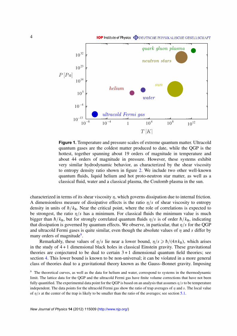
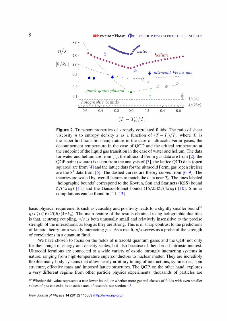
As shown in figure 1, strongly correlated quantum fluids cover a wide range of scales intemperature and pressure8. We remind the reader that temperature T and energy E are equivalentup to a factor of Boltzmann’s constant, kB = 1.3806503× 10−23 J K−1, with E = kBT . We focuson fluids that can be studied in bulk, as opposed to quantum liquids that exist on lattices. Weshow ultracold Fermi gases, liquid helium, neutron matter in proto-neutron stars and the QGP.For comparison we also show a classical fluid, water, and a classical plasma, the Coulombplasma in the sun.

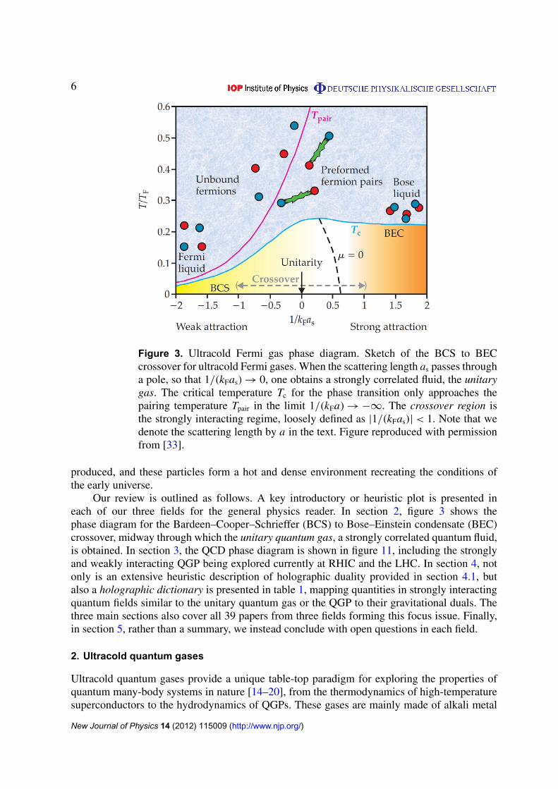
Figure 2 shows that despite the large range in scale there is a remarkable universality in thetransport behavior of strongly correlated quantum fluids. Transport properties of the fluid can be

7 Fluids are materials that obey the equations of hydrodynamics. The word liquid refers to a phase of matter thatcannot be distinguished from a gas in terms of symmetry, but exhibits short-range correlations similar to those in asolid, and is separated from the gas phase by a line of first-order transitions that terminates at a critical endpoint.A plasma is a gas of charged particles. Gases, liquids and plasmas behave as fluids if probed on very long lengthscales. Weakly coupled systems exhibit a single-particle behavior if probed on microscopic scales, but stronglycoupled systems behave like fluids also on short scales. Liquids are typically more strongly correlated than gases,and are more likely to behave like a fluid.8 The points in figure 1 correspond to the range of temperatures for which the transport measurements shownin figure 2 have been made. For the ultracold atomic Fermi gas experiments described in section 2.1 the criticaltemperature is roughly 500 nK (the exact value depends on the trap geometry and the number of particles; Bosegases have been cooled to temperatures below 1 nK). The data points for helium and water are centered aroundthe critical endpoint of the liquid gas transition. The point for the solar plasma corresponds to the geometric meanof the temperatures in the core and the corona. The neutron matter point is at T = 1 MeV/kB = 1.2× 1010 Kand at a density n = 0.1 n0, where n0 = 0.14 fm−3 is the nuclear matter saturation density. Neutron stars are bornat T ' 10 MeV/kB, and they can cool to temperatures below 1 keV/kB. The critical temperature of the QGP isTc ' 150 MeV/kB = 1.75× 1012 K. Experiments with heavy ions explore temperatures up to ∼ 3Tc.

New Journal of Physics 14 (2012) 115009 (http://www.njp.org/)

4

10 –8 10 –4 1 104 1081012

10–13

10 –4

105

1014

1023

1032

P [Pa]

T [K]

water

helium

ultracold Fermi gas

quark gluon plasma

neutron stars

sun

Figure 1. Temperature and pressure scales of extreme quantum matter. Ultracoldquantum gases are the coldest matter produced to date, while the QGP is thehottest, together spanning about 19 orders of magnitude in temperature andabout 44 orders of magnitude in pressure. However, these systems exhibitvery similar hydrodynamic behavior, as characterized by the shear viscosityto entropy density ratio shown in figure 2. We include two other well-knownquantum fluids, liquid helium and hot proto-neutron star matter, as well as aclassical fluid, water and a classical plasma, the Coulomb plasma in the sun.

characterized in terms of its shear viscosity η, which governs dissipation due to internal friction.A dimensionless measure of dissipative effects is the ratio η/s of shear viscosity to entropydensity in units of h/kB. Near the critical point, where the role of correlations is expected tobe strongest, the ratio η/s has a minimum. For classical fluids the minimum value is muchbigger than h/kB, but for strongly correlated quantum fluids η/s is of order h/kB, indicatingthat dissipation is governed by quantum effects. We observe, in particular, that η/s for the QGPand ultracold Fermi gases is quite similar, even though the absolute values of η and s differ bymany orders of magnitude9.

Remarkably, these values of η/s lie near a lower bound, η/s > h/(4πkB), which arisesin the study of 4 + 1 dimensional black holes in classical Einstein gravity. These gravitationaltheories are conjectured to be dual to certain 3 + 1 dimensional quantum field theories; seesection 4. This lower bound is known to be non-universal; it can be violated in a more generalclass of theories dual to a gravitational theory known as the Gauss–Bonnet gravity. Imposing

9 The theoretical curves, as well as the data for helium and water, correspond to systems in the thermodynamiclimit. The lattice data for the QGP and the ultracold Fermi gas have finite volume corrections that have not beenfully quantified. The experimental data point for the QGP is based on an analysis that assumes η/s to be temperatureindependent. The data points for the ultracold Fermi gas show the ratio of trap averages of η and s. The local valueof η/s at the center of the trap is likely to be smaller than the ratio of the averages; see section 5.1.

New Journal of Physics 14 (2012) 115009 (http://www.njp.org/)

5

0.6 0.4 0.2 0.0 0.2 0.4 0.6

0.1

0.2

0.5

1.0

2.0

5.0

waterhelium

ultracold Fermi gas

quark gluon plasma

holographic bounds1/(4π)

4/(25π)

Figure 2. Transport properties of strongly correlated fluids. The ratio of shearviscosity η to entropy density s as a function of (T − Tc)/Tc, where Tc isthe superfluid transition temperature in the case of ultracold Fermi gases, thedeconfinement temperature in the case of QCD and the critical temperature atthe endpoint of the liquid gas transition in the case of water and helium. The datafor water and helium are from [1], the ultracold Fermi gas data are from [2], theQGP point (square) is taken from the analysis of [3], the lattice QCD data (opensquares) are from [4] and the lattice data for the ultracold Fermi gas (open circles)are the 83 data from [5]. The dashed curves are theory curves from [6–9]. Thetheories are scaled by overall factors to match the data near Tc. The lines labeled‘holographic bounds’ correspond to the Kovtun, Son and Starinets (KSS) boundh/(4πkB) [11] and the Gauss–Bonnet bound (16/25)h/(4πkB) [10]. Similarcompilations can be found in [11–13].

basic physical requirements such as causality and positivity leads to a slightly smaller bound10

η/s > (16/25)h/(4πkB). The main feature of the results obtained using holographic dualitiesis that, at strong coupling, η/s is both unusually small and relatively insensitive to the precisestrength of the interactions, as long as they are strong. This is in sharp contrast to the predictionsof kinetic theory for a weakly interacting gas. As a result, η/s serves as a probe of the strengthof correlations in a quantum fluid.

We have chosen to focus on the fields of ultracold quantum gases and the QGP not onlyfor their range of energy and density scales, but also because of their broad intrinsic interest.Ultracold fermions are connected to a wide variety of exotic, strongly interacting systems innature, ranging from high-temperature superconductors to nuclear matter. They are incrediblyflexible many-body systems that allow nearly arbitrary tuning of interactions, symmetries, spinstructure, effective mass and imposed lattice structures. The QGP, on the other hand, exploresa very different regime from other particle physics experiments: thousands of particles are

10 Whether this value represents a true lower bound, or whether more general classes of fluids with even smallervalues of η/s can exist, is an active area of research; see section 4.3.

New Journal of Physics 14 (2012) 115009 (http://www.njp.org/)

6

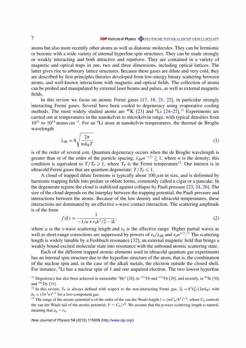
Figure 3. Ultracold Fermi gas phase diagram. Sketch of the BCS to BECcrossover for ultracold Fermi gases. When the scattering length as passes througha pole, so that 1/(kFas)→ 0, one obtains a strongly correlated fluid, the unitarygas. The critical temperature Tc for the phase transition only approaches thepairing temperature Tpair in the limit 1/(kFa)→−∞. The crossover region isthe strongly interacting regime, loosely defined as |1/(kFas)|< 1. Note that wedenote the scattering length by a in the text. Figure reproduced with permissionfrom [33].

produced, and these particles form a hot and dense environment recreating the conditions ofthe early universe.

Our review is outlined as follows. A key introductory or heuristic plot is presented ineach of our three fields for the general physics reader. In section 2, figure 3 shows thephase diagram for the Bardeen–Cooper–Schrieffer (BCS) to Bose–Einstein condensate (BEC)crossover, midway through which the unitary quantum gas, a strongly correlated quantum fluid,is obtained. In section 3, the QCD phase diagram is shown in figure 11, including the stronglyand weakly interacting QGP being explored currently at RHIC and the LHC. In section 4, notonly is an extensive heuristic description of holographic duality provided in section 4.1, butalso a holographic dictionary is presented in table 1, mapping quantities in strongly interactingquantum fields similar to the unitary quantum gas or the QGP to their gravitational duals. Thethree main sections also cover all 39 papers from three fields forming this focus issue. Finally,in section 5, rather than a summary, we instead conclude with open questions in each field.

2. Ultracold quantum gases

Ultracold quantum gases provide a unique table-top paradigm for exploring the properties ofquantum many-body systems in nature [14–20], from the thermodynamics of high-temperaturesuperconductors to the hydrodynamics of QGPs. These gases are mainly made of alkali metal

New Journal of Physics 14 (2012) 115009 (http://www.njp.org/)

7

atoms but also more recently other atoms as well as diatomic molecules. They can be fermionicor bosonic with a wide variety of internal hyperfine spin structures. They can be made stronglyor weakly interacting and both attractive and repulsive. They are contained in a variety ofmagnetic and optical traps in one, two and three dimensions, including optical lattices. Thelatter gives rise to arbitrary lattice structures. Because these gases are dilute and very cold, theyare described by first-principles theories developed from low-energy binary scattering betweenatoms, and well-known interactions with magnetic and optical fields. The collection of atomscan be probed and manipulated by external laser beams and pulses, as well as external magneticfields.

In this review we focus on atomic Fermi gases [17, 18, 21, 22], in particular stronglyinteracting Fermi gases. Several have been cooled to degeneracy using evaporative coolingmethods. The most widely studied atoms are 40K [23] and 6Li [24–27].11 Experiments arecarried out at temperatures in the nanokelvin to microkelvin range, with typical densities from1011 to 1014 atoms cm−3. For an 6Li atom at nanokelvin temperatures, the thermal de Brogliewavelength

λdB = h

√2π

mkBT(1)

is of the order of several µm. Quantum degeneracy occurs when the de Broglie wavelength isgreater than or of the order of the particle spacing, λdBn−1/3 & 1, where n is the density; thiscondition is equivalent to T/TF > 1, where TF is the Fermi temperature12. Our interest is inultracold Fermi gases that are quantum degenerate: T/TF 6 1.

A cloud of trapped dilute fermions is typically about 100µm in size, and is deformed byharmonic trapping fields into prolate or oblate forms, commonly called a cigar or a pancake. Inthe degenerate regime the cloud is stabilized against collapse by Pauli pressure [23, 24, 26]. Thesize of the cloud depends on the interplay between the trapping potential, the Pauli pressure andinteractions between the atoms. Because of the low density and ultracold temperatures, theseinteractions are dominated by an effective s-wave contact interaction. The scattering amplitudeis of the form

f (k)=1

−1/a + r0k2/2− ik, (2)

where a is the s-wave scattering length and r0 is the effective range. Higher partial waves aswell as short-range corrections are suppressed by powers of r0/λdB and r0n1/3.13 The scatteringlength is widely tunable by a Feshbach resonance [32], an external magnetic field that brings aweakly bound excited molecular state into resonance with the unbound atomic scattering state.

Each of the different trapped atomic elements used in ultracold quantum gas experimentshas an internal spin structure due to the hyperfine structure of the atom, that is, the combinationof the nuclear spin and, in the case of the alkali metals, the electron outside the closed shell.For instance, 6Li has a nuclear spin of 1 and one unpaired electron. The two lowest hyperfine

11 Degeneracy has also been achieved in metastable 3He∗ [28], in 171Yb and 173Yb [29], and recently, in 87Sr [30]and 161Dy [31].12 In this review, TF is always defined with respect to the non-interacting Fermi gas, TF = h2k2

F/(2mkB) withkF = (3π2n)1/3 for a two-component gas.13 The range of the atomic potential is of the order of the van der Waals length l = (mC6/h2)1/4, where C6 controlsthe van der Waals tail of the atomic potential, V ∼ C6/r6. We assume that the p-wave scattering length is natural,meaning that ap ∼ r0.

New Journal of Physics 14 (2012) 115009 (http://www.njp.org/)

8

states have a total spin of 1/2, and the remaining four have a total spin of 3/2. By selecting outhyperfine states through appropriate laser-induced transitions and trapping and cooling methods,experiments can thus work with a variety of spin structures. The case in which two hyperfinestates are trapped is effectively equivalent to a spin-1/2 atom. Tuning the scattering length byusing a Feshbach resonance, one obtains three distinct regimes, shown in figure 3. The first is forweak attractive scattering, −kFa� 1, where kF is the Fermi momentum. Then for temperatureswell below the Fermi temperature TF, one obtains a BCS state [34] or s-wave superconductivity.We call this an atomic Fermi superfluid, since our systems are in fact neutral. In such a state,fermions of opposite spin join to make Cooper pairs, but their average pair size ξc is greaterthan the interparticle spacing n−1/3, so that they are overlapping: ξcn1/3

� 1. Tuning a as in thephase diagram, we observe that the scattering length passes through a pole; note that the figureshows temperature as a function of the inverse scattering length, 1/(kFa). Thus as a→±∞,1/(kFa)→ 0, and one obtains a second regime, called the unitary gas. This middle regime is astrongly correlated fluid, and one finds that ξcn1/3

' 1, i.e. the pair size is approximately equalto the interparticle spacing. Finally, for large positive scattering lengths, the paired fermionsmake much more tightly bound molecules, and one obtains a molecular BEC, similar to thewell-known atomic BECs. This regime is depicted on the far right of figure 3. In practicethese molecules are still quite large, thousands of Bohr or more, but still much smaller thanthe interparticle spacing, so that ξcn1/3

� 1.The upper curve in the figure depicts the pair formation temperature Tpair, which in general

is distinct from the critical temperature for superfluidity, Tc [35]. Note that superfluidity isassociated with the spontaneous breakdown of a global symmetry, the U (1) phase symmetryof the wavefunction, and Tc is therefore always well defined. Tpair, on the other hand, is notassociated with a symmetry or a local order parameter and may not be well defined. This remarkis particularly relevant in the BCS regime, where the size of the pairs is large compared to theinterparticle spacing. Physically, we expect that in the BCS regime there are no pre-formedpairs, and Tc and Tpair are very close together.

Although we refer to these systems as ultracold, in terms of the dimensionless ratio T/TF,and in comparison with solid-state systems, they are quite hot. In the unitary regime the phasetransition occurs at Tc/TF = 0.167(23) [36], compared to typical solid state superconductors inwhich Tc/TF

<∼ 0.01. The unitary Fermi gas is a very high Tc superfluid. As indicated in figure 3,

in the BCS regime the temperature required for achieving a phase transition to an atomic Fermisuperfluid is quite low. In this regime, the critical temperature is given by the weak couplingexpression [37]

Tc

TF'

4× 21/3eγ

πe7/3exp

(−

π

kF|a|

), (3)

where γ ' 0.577 is the Euler constant. The numerical value of the factor in front of the exponentis 0.277. We observe that even though equation (3) is formally valid only in the limit kF|a| � 1,it also provides a reasonable estimate for Tc at unitarity. This is somewhat of an accident,because higher order corrections in kF|a| are divergent in the unitary limit.

In the following, we explore the unitary regime of the BCS–BEC crossover for ultracoldFermi gases. In section 2.1 we present an overview of experiments on these systems. Insection 2.2 we focus on universal aspects of unitary gases. In the strongly correlated regime thescattering length diverges, and the remaining length scales in the problem are the Fermi length1/kF and the de Broglie wavelength λdB, given in equation (1). Thus many theoretical statements

New Journal of Physics 14 (2012) 115009 (http://www.njp.org/)

9

can be made despite the lack of a small parameter or perturbative calculations. In sections 2.3and 2.4, we treat the thermodynamics and the structure of the phase diagram for unitary gases,and in section 2.5 we focus on transport properties. Section 2.6 presents an overview of ultracoldFermi gases in optical lattices. Finally, in section 2.7 we treat new directions in unitary gases aspresented in this focus issue, including novel experimental probes, solitons, imbalanced systemsand polarons, disorder, quantum phase transitions, Efimov physics and the use of three hyperfinestates to explore SU(3) physics and connections to the QGP.

2.1. Ultracold Fermi gas experiments

Historically, atomic Fermi gases were first brought to degeneracy at JILA in 1999 [23],using a mixture of two hyperfine states in 40K to enable s-wave scattering in a magnetictrap. Dual species radio-frequency (RF)-induced evaporation produced a degenerate, weaklyinteracting sample, with T/TF ' 0.5. Later, degeneracy was achieved in fermionic 6Li by directevaporation from a magneto-optical trap (MOT)-loaded optical trap [26] and by sympatheticcooling with another species [24, 25, 27], producing a lower T/TF. However, the minimumreduced temperature was initially limited to T/TF ' 0.2, which may have been a consequenceof trap-noise-induced heating [40] or, at the lowest temperatures, Fermi hole heating [38] incombination with evaporative cooling [39].

Optical traps enabled a dramatic improvement in the efficiency of evaporation and thecreation of strongly interacting Fermi gases, through the use of magnetically tunable collisionalresonances or Feshbach resonances [41]. Feshbach resonances in fermionic atoms were initiallycharacterized in 2002 by several groups [42–44]. For a recent review of Feshbach resonancessee [32]. In a Feshbach resonance, a bias magnetic field tunes the total energy of a pairof colliding atoms in the incoming open (triplet) channel into resonance with a molecularbound state in an energetically closed (singlet) channel. At resonance, the zero-energy s-wavescattering length a diverges and the collision cross section attains the unitary limit, proportionalto the square of the de Broglie wavelength, i.e. σ = 4π/k2, where hk is the relative momen-tum. The collision cross section therefore increases with decreasing temperature, enablinghighly efficient evaporative cooling in optical traps and much lower reduced temperaturesT/TF ' 0.05.

An optical trap is formed by a focused laser beam. Atoms are polarized by the fieldand attracted to the high-intensity region when the laser is detuned below resonance withthe resonant optical transition, so that the induced dipole moment is in phase with the field.For large detunings, obtained using infrared lasers, the trapping potential is independent ofthe atomic hyperfine state, enabling several species to be trapped, which is ideal for Fermigases [45]. Forced evaporation is accomplished by slowly lowering the intensity of the opticaltrap laser beam. Near a Feshbach resonance, a highly degenerate sample can be produced in afew seconds [46].

A milestone in the Fermi gas field was the observation in 2002 of a strongly interacting,degenerate Fermi gas [46], in the so-called BEC–BCS crossover regime, using this method. Incontrast to Bose gases, which are unstable and undergo three-body loss on millisecond timescales near Feshbach resonances, the two-component Fermi gas was found to be stable, as thePauli principle suppresses three-body s-wave scattering [47]. Released from the cigar-shapedtrapping potential of the focused beam, the cloud was observed to expand much more rapidlyin the initially narrow direction, compared to the long direction, as a consequence of the muchlarger pressure gradient along the narrow axis. Consequently, the aspect ratio inverts from a cigar

New Journal of Physics 14 (2012) 115009 (http://www.njp.org/)

10

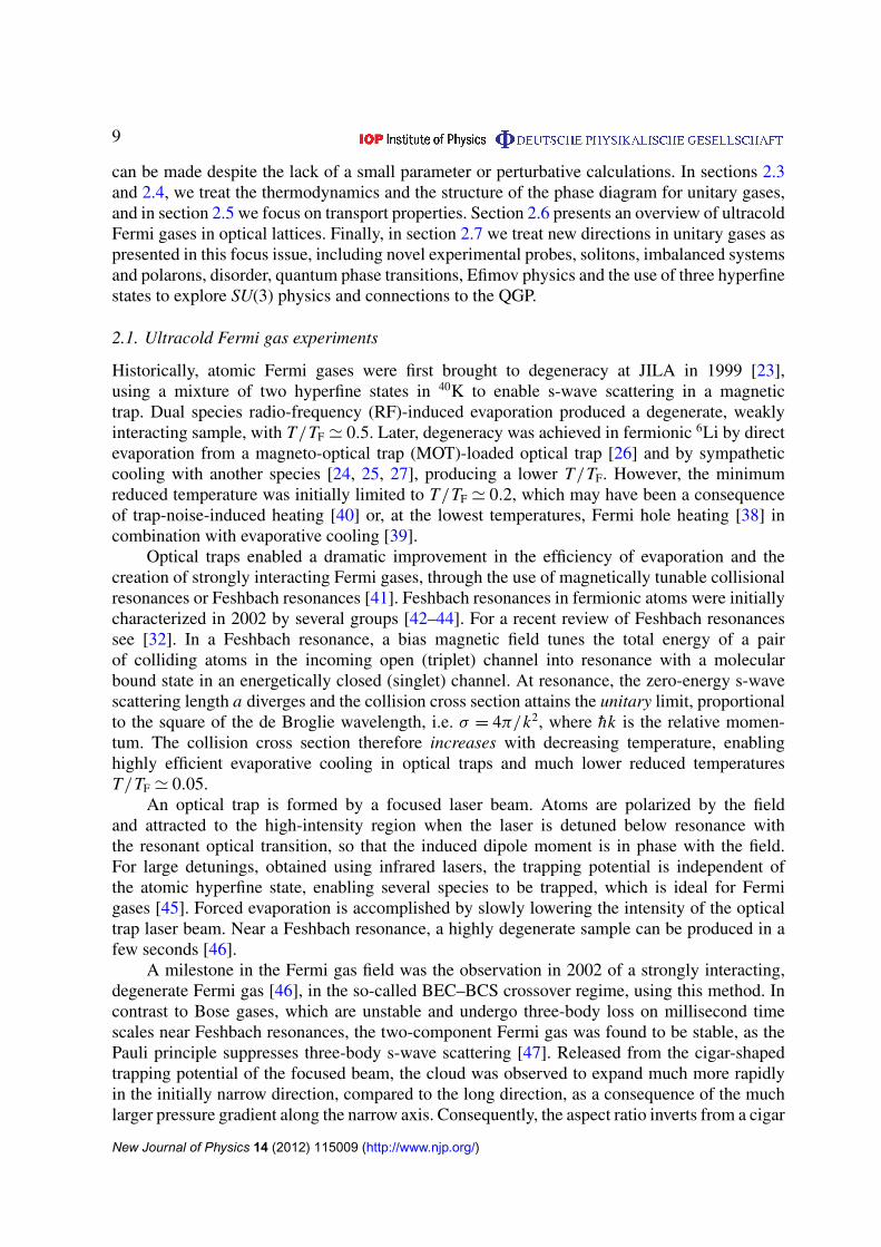
Figure 4. Experimental images. Elliptic flow of a strongly interacting Fermi gasas a function of time after release from a cigar-shaped optical trap: from top tobottom, 100µs to 2 ms after release. The pressure gradient is much larger in theinitially narrow directions of the cloud than in the long direction, causing thegas to expand much more rapidly along the initially narrow directions, invertingthe aspect ratio. Achieving a nearly perfect elliptic flow requires extremely lowshear viscosity, as is the case for a QGP. The sequence of images is createdby recreating similar initial conditions and destructively imaging the cloud atdifferent times after release [46].

to an ellipse, as shown in figure 4. Remarkably, the same type of elliptic flow is also observedin the momentum distribution of an expanding QGP produced in an off-center collision of twoheavy ions; see section 3.5. There, the temperature is 19 orders of magnitude hotter and theparticle density is 25 orders of magnitude greater than that of the Fermi gas. In both systems,however, this nearly perfect ‘elliptic’ flow, figure 4, is a consequence of extremely low-viscosityhydrodynamics, which persists in the normal, non-superfluid unitary gas and deeply connectsthese two apparently disparate fields.

The creation of a degenerate Fermi gas near a Feshbach resonance was followed in 2003by the first measurements of the interaction energy [48, 49] and the creation of Bose-condenseddimer molecules [50–53]. In 2004, condensed fermionic atom pairs were observed using a fastmagnetic field sweep to project the pairs onto stable molecular dimers [54, 55]. Using thismethod, the first phase diagram in the crossover region was obtained (see figure 3) as a functionof magnetic field and temperature, albeit using the temperature of the ideal gas obtained byan adiabatic sweep to a non-interacting regime [54]. Evidence for superfluidity in a Fermi gas

New Journal of Physics 14 (2012) 115009 (http://www.njp.org/)

11

was provided by the measurement of collective mode frequencies and damping rates versustemperature [56] and magnetic field [57], and by the measurement of the pairing gap by RFspectroscopy [58]. The observation of a vortex lattice in 2005 provided a direct verification ofFermi superfluid behavior [59].

Also in 2005, initial thermodynamic measurements were made by adding a controlledamount of energy to the cloud and measuring an empirical temperature from the correspondingcloud spatial profile [60]. However, the results were model dependent, as the calibration ofthe empirical temperature relied on comparing the measured cloud profiles with theoreticalpredictions. Model-independent measurements were soon to follow, based on universal behaviorin the unitary regime, where the local thermodynamic quantities, such as pressure, are functionsonly of the density n and the temperature T [61].

Model-independent measurements of the total energy E of a resonantly interactingFermi gas are based on the Virial theorem, which holds for a unitary gas as a consequenceof universality and yields the energy directly from the cloud profile [62]. Using entropiccooling [63, 64], a model-independent measurement of the total entropy S was accomplishedby an adiabatic sweep of the bias magnetic field from resonance to the weakly interactingregime, where the entropy can be calculated from the cloud profile [65]. As T = ∂E/∂S, thesemeasurements enabled the first model-independent temperature calibration and estimates of thecritical parameters in the strongly interacting regime [66]. A refined temperature calibration isused in the measurement of universal quantum viscosity, as described in this focus issue [2].

Measurements of global thermodynamic quantities from the cloud profiles in thestrongly interacting regime are now superseded by model-independent measurements of localquantities [67, 68]. Using the Gibbs–Duhem relation

dP = n dµ (4)

at constant temperature, the local pressure is obtainable from the integrated column density,where the local chemical potential µ is determined by the known trap potential [69, 70].Combined with a temperature measurement, the local equation of state P(µ, T ) or P(n, T )is determined. The most precise local measurements avoid temperature measurement, whichintroduces the most uncertainty, by determining the pressure, density and compressibilityfrom the cloud profiles. The resulting equation of state reveals clearly a lambda transition,and provides the best measurement of the critical parameters for a unitary Fermi gas [36],as described in detail in section 2.3. Measurements of equilibrium thermodynamic quantitiesare now used as stringent tests of predictions, as described in this focus issue by Hu andco-workers [71]. These thermodynamic measurements are connected to universal hydrodynam-ics and transport measurements, as described in [2].

We proceed to describe the all-optical methods developed at Duke in 2002 [26, 46], as onespecific example of experimental techniques, which are closely tied to the theme of this focusissue, namely viscosity and transport measurements on Fermi gases in the universal regime [2].A degenerate, strongly interacting Fermi gas is readily made by all-optical methods [46]. Assketched in the left panel of figure 5, an MOT is used to pre-cool a 50 : 50 mixture of spin-up and spin-down 6Li atoms, which is loaded into a CO2 laser optical trap and magneticallytuned to an s-wave Feshbach resonance. Atoms from the source (lower right, green cylinder)form an atomic beam (blue arrow) that is slowed by radiation pressure forces from a resonantlaser beam (top left, opposing red arrow). For 6Li, the deceleration is 2× 106 m s−2, slowing theatoms from oven thermal speeds of 1 km s−1 to tens of m s−1 over a distance of a fraction of ameter. Six laser beams (three thick red lines) then propagate toward the center of the MOT

New Journal of Physics 14 (2012) 115009 (http://www.njp.org/)

12

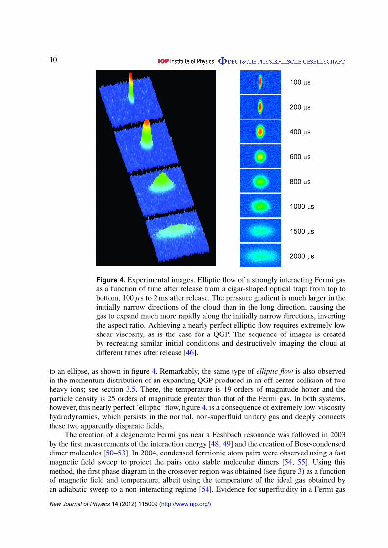
Figure 5. Ultracold quantum gas experimental apparatus. Left: sketch of theexperimental apparatus for ultracold fermions. Right: apparatus for the Dukeexperiments (currently at North Carolina State University). Compare to a sketchof the QGP experiment at the LHC in figure 12: the quantum gas experiment isabout ten times smaller (2.5 versus 26 m), but the size of the trapped ultracoldgas is 11 orders of magnitude larger (a few hundreds of micrometers versus a fewfemtometers). The ultracold quantum gas is at nanokelvin temperatures, or pico-eV, compared to the deconfinement temperature of ' 2× 1012 K in the QGP, or200 MeV, created by colliding gold nuclei at energies of 100 GeV per nucleon.

(point of intersection of three thick red lines), creating inward damping forces that cool theatoms. Opposing magnetic fields, created by two coils (stacked black circles, top and bottom),spatially tune the atomic resonance frequency, causing the six beams to produce a harmonicrestoring force at the MOT center. Typical MOT clouds are a few millimeters across andcontain several hundreds of million atoms. A trapping laser beam (shown in yellow) is focused(lenses indicated by two light blue ovals) at the MOT center and loaded. After turning off theMOT beams and the MOT magnetic field, an additional bias magnetic field tunes the atomsto a collisional (Feshbach) resonance. Forced evaporation near resonance, by lowering thetrap depth, rapidly cools the cloud to quantum degeneracy, i.e. T/TF� 1, producing a cigar-shaped cloud that is typically a few microns in diameter and several hundreds of microns long,containing several hundred thousands of atoms. In the right panel of figure 5 is shown theexperimental apparatus from the Duke laboratory, currently located at North Carolina StateUniversity. From right to left in the photo: the oven assembly where hot fermions are produced(aluminum housing); the camera to produce density images (blue device in the foreground); aZeeman slower to bring atoms into MOT (middle, behind camera); bias field magnets containingMOT in ultrahigh vacuum (white plastic housings); ZnSe lens for the CO2 laser trapping beamand optical table (left).

In the simplest case, the optical trap consists of a single laser beam, focused into the centerof the MOT and detuned well below the atomic resonance frequency to suppress spontaneousscattering, which would otherwise heat the atoms. For an optical trapping laser detuned belowthe atomic resonance, the induced atomic dipole moment is in-phase with the trapping laserfield, so that the atoms are attracted to the high-field region at the trap focus, i.e. the effectivetrapping potential is U =−α〈E2

〉/2, where the polarizability α > 0 and 〈E2〉 is proportional to

the trap laser intensity, time averaged over a few optical cycles. The effective potential then hasthe same spatial profile as the intensity of the focused trap laser. For ultracold atoms, the energy

New Journal of Physics 14 (2012) 115009 (http://www.njp.org/)

13

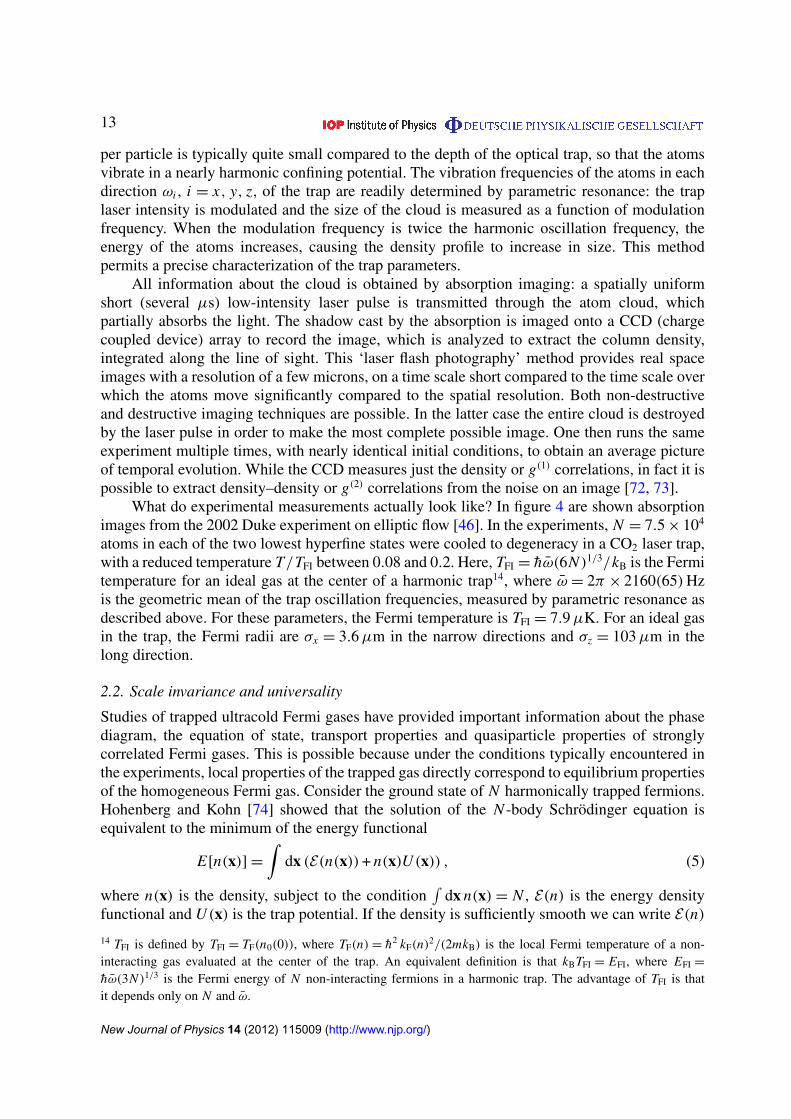
per particle is typically quite small compared to the depth of the optical trap, so that the atomsvibrate in a nearly harmonic confining potential. The vibration frequencies of the atoms in eachdirection ωi , i = x, y, z, of the trap are readily determined by parametric resonance: the traplaser intensity is modulated and the size of the cloud is measured as a function of modulationfrequency. When the modulation frequency is twice the harmonic oscillation frequency, theenergy of the atoms increases, causing the density profile to increase in size. This methodpermits a precise characterization of the trap parameters.

All information about the cloud is obtained by absorption imaging: a spatially uniformshort (several µs) low-intensity laser pulse is transmitted through the atom cloud, whichpartially absorbs the light. The shadow cast by the absorption is imaged onto a CCD (chargecoupled device) array to record the image, which is analyzed to extract the column density,integrated along the line of sight. This ‘laser flash photography’ method provides real spaceimages with a resolution of a few microns, on a time scale short compared to the time scale overwhich the atoms move significantly compared to the spatial resolution. Both non-destructiveand destructive imaging techniques are possible. In the latter case the entire cloud is destroyedby the laser pulse in order to make the most complete possible image. One then runs the sameexperiment multiple times, with nearly identical initial conditions, to obtain an average pictureof temporal evolution. While the CCD measures just the density or g(1) correlations, in fact it ispossible to extract density–density or g(2) correlations from the noise on an image [72, 73].

What do experimental measurements actually look like? In figure 4 are shown absorptionimages from the 2002 Duke experiment on elliptic flow [46]. In the experiments, N = 7.5× 104

atoms in each of the two lowest hyperfine states were cooled to degeneracy in a CO2 laser trap,with a reduced temperature T/TFI between 0.08 and 0.2. Here, TFI = hω(6N )1/3/kB is the Fermitemperature for an ideal gas at the center of a harmonic trap14, where ω = 2π × 2160(65)Hzis the geometric mean of the trap oscillation frequencies, measured by parametric resonance asdescribed above. For these parameters, the Fermi temperature is TFI = 7.9µK. For an ideal gasin the trap, the Fermi radii are σx = 3.6µm in the narrow directions and σz = 103µm in thelong direction.

2.2. Scale invariance and universality

Studies of trapped ultracold Fermi gases have provided important information about the phasediagram, the equation of state, transport properties and quasiparticle properties of stronglycorrelated Fermi gases. This is possible because under the conditions typically encountered inthe experiments, local properties of the trapped gas directly correspond to equilibrium propertiesof the homogeneous Fermi gas. Consider the ground state of N harmonically trapped fermions.Hohenberg and Kohn [74] showed that the solution of the N -body Schrodinger equation isequivalent to the minimum of the energy functional

E[n(x)]=∫

dx (E(n(x))+ n(x)U (x)) , (5)

where n(x) is the density, subject to the condition∫

dx n(x)= N , E(n) is the energy densityfunctional and U (x) is the trap potential. If the density is sufficiently smooth we can write E(n)14 TFI is defined by TFI = TF(n0(0)), where TF(n)= h2 kF(n)2/(2mkB) is the local Fermi temperature of a non-interacting gas evaluated at the center of the trap. An equivalent definition is that kBTFI = EFI, where EFI =

hω(3N )1/3 is the Fermi energy of N non-interacting fermions in a harmonic trap. The advantage of TFI is thatit depends only on N and ω.

New Journal of Physics 14 (2012) 115009 (http://www.njp.org/)

14

as a function of the local density and its gradients. On dimensional grounds we have

E(n(x))=c0h2

mn(x)5/3 +

c1h2

m

( E∇n(x))2

n(x)+ O

(∇

4n(x)), (6)

where c0, c1, . . . are dimensionless constants. At unitarity the coefficients ci are pure numbers,but for a finite scattering length they become functions of na3. To first approximation wecan neglect the gradient terms. Then the density is given by n(x)= neq(µ−U (x)), whereneq(µ) is the equilibrium density at the chemical potential µ and zero temperature. Thisapproximation is known as the local density approximation. Gradient terms are suppressed by(ω⊥/µ)

2∼ 1/(λz N )2/3, where λz = ωz/ω⊥ is the trap deformation. Typical experiments involve

λz ' 0.025–0.1 and N > 105, so corrections beyond the local density approximation are quitesmall. These arguments generalize to systems at non-zero temperature. In this case the densityof the trapped system is n(x)= neq(µ−U (x), T ).

The equilibrium density can be determined from the equation of state, P = P(µ, T ),through the thermodynamic relation15 n = ∂P/∂µ. In the following we also frequently refer tothe relation P = P(n, T ) as the equation of state. At unitarity the interaction is scale invariantand the only scales in the many-body system are the interparticle distance n−1/3 and thede Broglie wavelength, given in equation (1). Dimensional analysis implies that the equationof state must be of the form

P(n, T )=h2n5/3

mf (nλ3

dB), (7)

where f (x) is a universal function. At zero temperature the pressure is proportional to n5/3/m.This implies, in particular, that the pressure is given by a numerical constant times the pressureof a free Fermi gas. The same is true of the energy per particle and the chemical potential. Ithas become standard to denote the ratio of the energy per particle of the unitary gas and the freeFermi gas as the Bertsch parameter ξ ,

E

N= ξ

(E

N

)0

. (8)

Bertsch posed the calculation of the parameter ξ as a challenge problem to the many-bodyphysics community in 1999 [75]. At the time, the problem was stated in the context of a toymodel for dilute neutron matter; see section 3.1.

Using thermodynamic identities we can show that equation (7) implies that P = 23ε, where

ε is the energy density. This relation is analogous to the equation of state of a scale-invariantrelativistic gas, P = 1

3ε, as discussed in section 3.2. For a trapped gas the relation betweenpressure and energy density implies a Virial theorem: in a harmonic trap, the internal energy ofthe system is equal to the potential energy of the trapping potential [76, 77],∫

dx ε(x)=∫

dx n(x)U (x). (9)

These universal relations have been extended in many ways; see [78] for a review. An importantclass of relations, discovered by Tan, connects the derivative of thermodynamic quantities withrespect to 1/a to short-range correlation in the gas. Tan defined the contact density C via [79–81]

dε

d(a−1)=−

h2

4πmC, (10)

15 Here and in the remainder of this review we have dropped the subscript ‘eq’.

New Journal of Physics 14 (2012) 115009 (http://www.njp.org/)

15

where the derivative is taken at constant entropy density. The contact density appears in anumber of thermodynamic relations. The universal equation of state, for example, is given by

P =2

3ε +

h2

12πmaC. (11)

More remarkable is the fact that C controls short-distance correlations in the dilute Fermi gas.The tail of the momentum distribution is given by

nσ (k)→C

k4

(|a|−1

� k� r−10

), (12)

where C =∫

d3x C(x) is the integrated contact, nσ (k) is the momentum distribution16 in the spinstate σ and r0 is the range of the interaction. There are similar expressions for the asymptoticbehavior of other correlation observables such as the static and dynamic structure factors, andthe dynamic shear viscosity; see [82] for a review. In this focus issue, Kuhnle et al [83] presenta comprehensive set of measurements of the contact as a function of interaction strength andreduced temperature. These results can be compared to new theoretical predictions discussedby Hu and co-workers [71].

Below the critical temperature for superfluidity, the superfluid flow velocity vs can beviewed as an additional thermodynamic variable. The response of the pressure to the superfluidvelocity defines the superfluid mass density

ρs = mns =−∂2 P

∂v2s

∣∣∣∣vn=0

, (13)

where the derivative is taken in the rest frame of the normal fluid, meaning that vn = 0. Thesuperfluid mass density can be measured using rotating clouds [84]. The second moment of thetrap integrated value of the superfluid mass density determines the quenching of the moment ofinertia. New measurements of the moment of inertia can be found in [85].

For small values of n|a|3 the equation of state P(n, T ) can be computed in perturbationtheory. This program was initiated by Lee and Yang [86] and Huang and Yang [87]. At unitarity,weak coupling methods can be used in the limit of high temperature. This is based on theobservation that the binary cross section at unitarity is σ = 4π/k2. At high temperature themean momentum is large and the average thermal cross section is small. The equation of statecan be written as an expansion in nλ3

dB, which is the well-known Virial expansion. We have

P = nkBT{1 + b2(nλ

3dB)+ O((nλ3

dB)2)}, (14)

with b2 =−1/(2√

2) at unitarity [88, 89]. Analytic approaches in the non-perturbative regimenλ3

dB ∼ 1 are based on extrapolating to the unitary limit from different regimes in the phasediagram. For this purpose the phase diagram has been studied as a function of the strength ofthe interaction, the number of species and the number of spatial dimensions. The oldest theoryof this type is the Nozieres–Schmitt–Rink (NSR) theory [90–92], which is based on a set ofmany-body diagrams that correctly describe both the BCS and BEC limits. NSR theory workssurprisingly well, despite the formal lack of a small parameter at unitarity. For example, the basicform of the critical temperature sketched in figure 3 is correctly reproduced. Modern theories ofthis type are typically based on self-consistent T -matrix approximations; see [93, 94]. Anotheridea is to generalize the unitary Fermi gas to 2N spin states [95]. Mean field theory is reliable

16 The momentum distribution is normalized as∫

dk/(2π)3nσ (k)= Nσ , where Nσ is the total number of atoms inthe state σ .

New Journal of Physics 14 (2012) 115009 (http://www.njp.org/)

16

in the limit N →∞, and the interesting case N = 1 can be studied by expanding in 1/N . Thismethod is of interest in connection with holographic dualities, because the gravitational dualis expected to be classical in the limit that the number of degrees of freedom is large. Finally,it was proposed to use the number of dimensions as a control parameter. The unitary limit isperturbative in both D = 2 and 4 spatial dimensions [96]. The interesting case D = 3 can bestudied as an expansion around D = 2 + ε or 4− ε dimensions [97].

These methods are promising, but currently the only techniques that provide reliable andsystematically improvable results in the regime nλ3

dB ' 1 are quantum Monte Carlo calculations.At zero temperature the standard technique is Green function Monte Carlo [98, 99]. This methodrelies on a variational initial wavefunction, which is used as the initial condition for an imaginarytime diffusion process. The Monte Carlo method suffers from a fermion sign problem which isaddressed using the fixed node approximation. At finite temperature a number of groups haveperformed imaginary time path integral Monte Carlo calculations [100–103]. These calculationsdo not rely on variational input, and they do not suffer from a sign problem, but they areformulated on a space–time lattice and require an extrapolation to zero lattice spacing. Onenew technique is bold diagrammatic Monte Carlo, which is based on sampling the sum of allFeynman diagrams. The method suffers from a sign problem, but convergence in the regimeabove the critical temperature for superfluidity was found to be very good [104].

2.3. Experimental determination of the equation of state

The equation of state describes a functional relation between key thermodynamic variables,such as the pressure P(µ, T ) as a function of chemical potential µ and temperature T . In Fermigases, as stated in section 2.1, what we can actually measure is the density profile of a trappedcloud. There are various techniques for translating density measurements into thermodynamicquantities, all relying on the local density approximation.

The first thermodynamic measurements took place at Duke in 2005, where globalthermodynamic variables were measured. In the initial experiments [60], a controlled amount ofenergy was added to the trapped cloud by abruptly releasing it from the optical trap, allowing itto expand hydrodynamically by a known factor, and then recapturing the cloud after a selectedexpansion time, thereby increasing the potential energy. After allowing the gas to equilibrate, thecloud profile was measured to determine an empirical temperature, which was later calibratedby comparing to theoretical cloud profiles, predicted as a function of reduced temperature. Theresulting energy versus temperature curve was compared to that measured for an ideal Fermigas in the same trap, and showed a departure from ideal gas behavior at a certain temperature,which yielded an estimate of the superfluid-to-normal fluid transition temperature. However, theresults suffered from being model dependent, as calibration of the empirical temperature reliedon a comparison of the measured cloud profiles with theoretical predictions. To avoid this modeldependence, in 2006 the JILA group measured the potential energy of the strongly interactingcloud of 40K as a function of the ideal Fermi gas temperature that was obtained after an adiabaticsweep of the bias field to the non-interacting regime above resonance [105].

Model-independent determination of thermodynamic quantities was done by the Dukegroup in 2007 [65], where the total energy E and the total entropy S of a trapped cloud weremeasured from cloud profiles, by exploiting the universal behavior of a unitary Fermi gas at aFeshbach resonance. From equation (9) we know that for a harmonic trapping potential the totalenergy is twice the average potential energy, E = 2〈U 〉 = 3 mω2

z 〈z2〉. Hence, by measuring the

harmonic oscillator frequency and mean square cloud size, the total energy is readily determined

New Journal of Physics 14 (2012) 115009 (http://www.njp.org/)

17

4

3

2

1

0

E/E

F

76543210S/kB

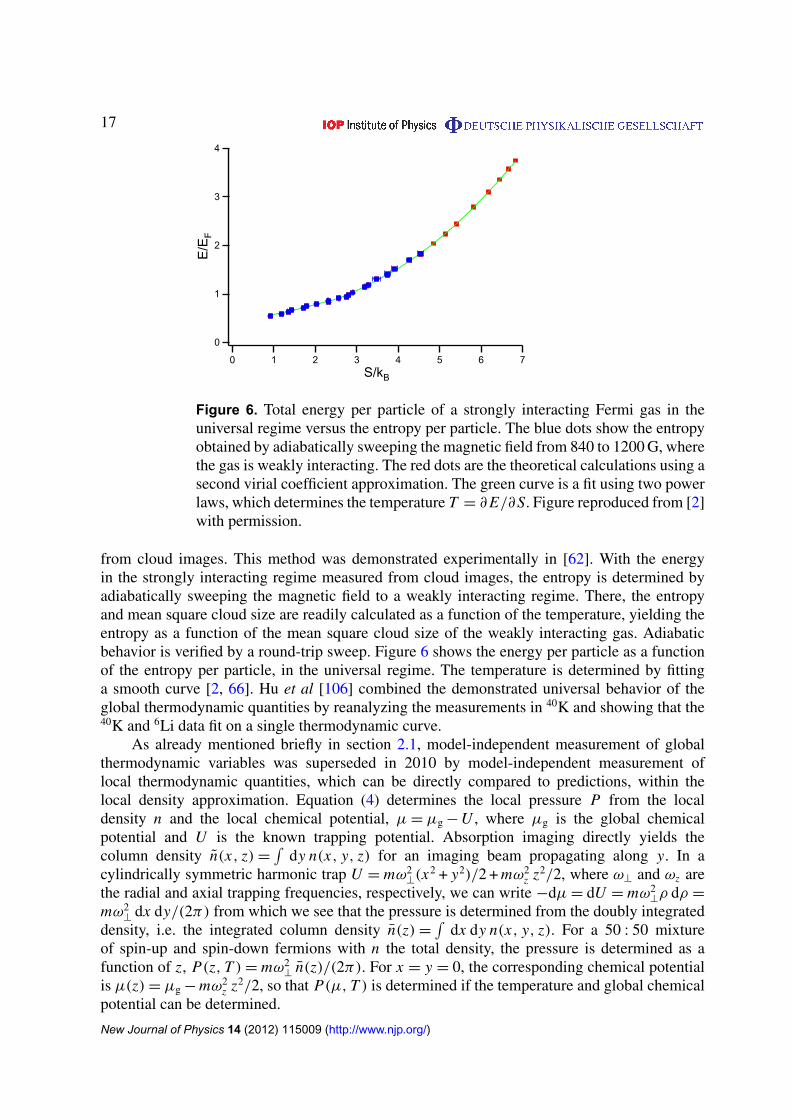
Figure 6. Total energy per particle of a strongly interacting Fermi gas in theuniversal regime versus the entropy per particle. The blue dots show the entropyobtained by adiabatically sweeping the magnetic field from 840 to 1200 G, wherethe gas is weakly interacting. The red dots are the theoretical calculations using asecond virial coefficient approximation. The green curve is a fit using two powerlaws, which determines the temperature T = ∂E/∂S. Figure reproduced from [2]with permission.

from cloud images. This method was demonstrated experimentally in [62]. With the energyin the strongly interacting regime measured from cloud images, the entropy is determined byadiabatically sweeping the magnetic field to a weakly interacting regime. There, the entropyand mean square cloud size are readily calculated as a function of the temperature, yielding theentropy as a function of the mean square cloud size of the weakly interacting gas. Adiabaticbehavior is verified by a round-trip sweep. Figure 6 shows the energy per particle as a functionof the entropy per particle, in the universal regime. The temperature is determined by fittinga smooth curve [2, 66]. Hu et al [106] combined the demonstrated universal behavior of theglobal thermodynamic quantities by reanalyzing the measurements in 40K and showing that the40K and 6Li data fit on a single thermodynamic curve.

As already mentioned briefly in section 2.1, model-independent measurement of globalthermodynamic variables was superseded in 2010 by model-independent measurement oflocal thermodynamic quantities, which can be directly compared to predictions, within thelocal density approximation. Equation (4) determines the local pressure P from the localdensity n and the local chemical potential, µ= µg−U , where µg is the global chemicalpotential and U is the known trapping potential. Absorption imaging directly yields thecolumn density n(x, z)=

∫dy n(x, y, z) for an imaging beam propagating along y. In a

cylindrically symmetric harmonic trap U = mω2⊥(x2 + y2)/2 + mω2

z z2/2, where ω⊥ and ωz arethe radial and axial trapping frequencies, respectively, we can write −dµ= dU = mω2

⊥ρ dρ =

mω2⊥

dx dy/(2π) from which we see that the pressure is determined from the doubly integrateddensity, i.e. the integrated column density n(z)=

∫dx dy n(x, y, z). For a 50 : 50 mixture

of spin-up and spin-down fermions with n the total density, the pressure is determined as afunction of z, P(z, T )= mω2

⊥n(z)/(2π). For x = y = 0, the corresponding chemical potential

is µ(z)= µg−mω2z z2/2, so that P(µ, T ) is determined if the temperature and global chemical

potential can be determined.

New Journal of Physics 14 (2012) 115009 (http://www.njp.org/)

18

2.0

1.8

1.6

1.4

1.2

1.0

0.8

0.6

0.4

E/E

F

0.80.60.40.20.0

T/TFI

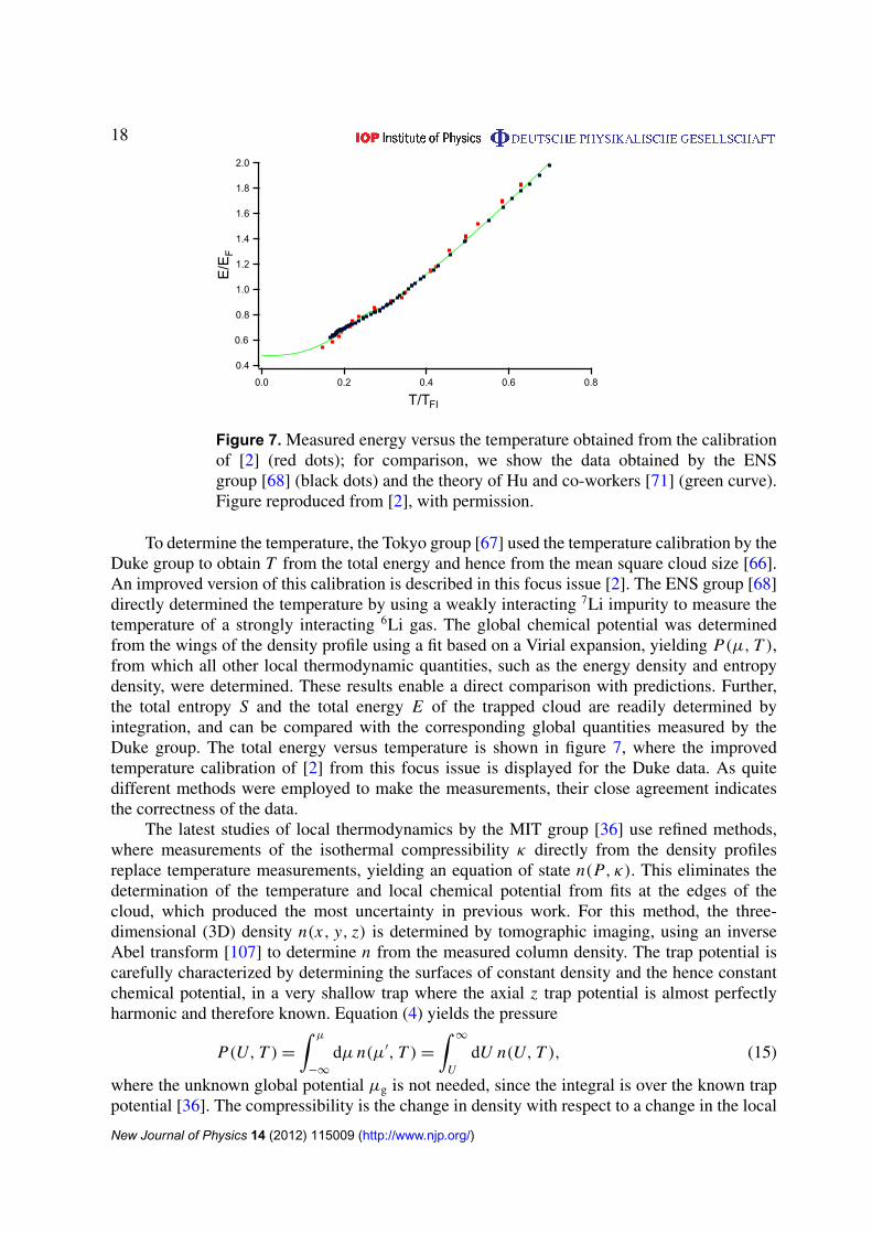
Figure 7. Measured energy versus the temperature obtained from the calibrationof [2] (red dots); for comparison, we show the data obtained by the ENSgroup [68] (black dots) and the theory of Hu and co-workers [71] (green curve).Figure reproduced from [2], with permission.

To determine the temperature, the Tokyo group [67] used the temperature calibration by theDuke group to obtain T from the total energy and hence from the mean square cloud size [66].An improved version of this calibration is described in this focus issue [2]. The ENS group [68]directly determined the temperature by using a weakly interacting 7Li impurity to measure thetemperature of a strongly interacting 6Li gas. The global chemical potential was determinedfrom the wings of the density profile using a fit based on a Virial expansion, yielding P(µ, T ),from which all other local thermodynamic quantities, such as the energy density and entropydensity, were determined. These results enable a direct comparison with predictions. Further,the total entropy S and the total energy E of the trapped cloud are readily determined byintegration, and can be compared with the corresponding global quantities measured by theDuke group. The total energy versus temperature is shown in figure 7, where the improvedtemperature calibration of [2] from this focus issue is displayed for the Duke data. As quitedifferent methods were employed to make the measurements, their close agreement indicatesthe correctness of the data.

The latest studies of local thermodynamics by the MIT group [36] use refined methods,where measurements of the isothermal compressibility κ directly from the density profilesreplace temperature measurements, yielding an equation of state n(P, κ). This eliminates thedetermination of the temperature and local chemical potential from fits at the edges of thecloud, which produced the most uncertainty in previous work. For this method, the three-dimensional (3D) density n(x, y, z) is determined by tomographic imaging, using an inverseAbel transform [107] to determine n from the measured column density. The trap potential iscarefully characterized by determining the surfaces of constant density and the hence constantchemical potential, in a very shallow trap where the axial z trap potential is almost perfectlyharmonic and therefore known. Equation (4) yields the pressure

P(U, T )=∫ µ

−∞

dµ n(µ′, T )=∫∞

UdU n(U, T ), (15)

where the unknown global potential µg is not needed, since the integral is over the known trappotential [36]. The compressibility is the change in density with respect to a change in the local

New Journal of Physics 14 (2012) 115009 (http://www.njp.org/)

19

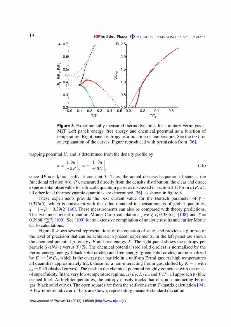
Figure 8. Experimentally measured thermodynamics for a unitary Fermi gas atMIT. Left panel: energy, free energy and chemical potential as a function oftemperature. Right panel: entropy as a function of temperature. See the text foran explanation of the curves. Figure reproduced with permission from [36].

trapping potential U , and is determined from the density profile by

κ =1

n

∂n

∂P

∣∣∣∣T

=−1

n2

∂n

∂U

∣∣∣∣T

, (16)

since dP = n dµ=−n dU at constant T . Thus, the actual observed equation of state is thefunctional relation n(κ, P), measured directly from the density distribution, the clear and directexperimental observable for ultracold quantum gases as discussed in section 2.1. From n(P, κ),all other local thermodynamic quantities are determined [36], as shown in figure 8.

These experiments provide the best current value for the Bertsch parameter of ξ =0.376(5), which is consistent with the value obtained in measurements of global quantities,ξ = 1 +β = 0.39(2) [66]. These measurements can also be compared with theory predictions.The two most recent quantum Monte Carlo calculations give ξ 6 0.383(1) [108] and ξ =

0.3968+0.0076−0.0077 [109]. See [109] for an extensive compilation of analytic results and earlier Monte

Carlo calculations.Figure 8 shows several representations of the equation of state, and provides a glimpse of

the level of precision that can be achieved in present experiments. In the left panel are shownthe chemical potential µ, energy E and free energy F . The right panel shows the entropy perparticle S/(NkB) versus T/TF. The chemical potential (red solid circles) is normalized by theFermi energy; energy (black solid circles) and free energy (green solid circles) are normalizedby E0 =

35 N EF, which is the energy per particle in a uniform Fermi gas. At high temperatures

all quantities approximately track those for a non-interacting Fermi gas, shifted by ξn − 1 withξn ' 0.45 (dashed curves). The peak in the chemical potential roughly coincides with the onsetof superfluidity. In the very low-temperature regime,µ/EF, E/E0 and F/F0 all approach ξ (bluedashed line). At high temperatures, the entropy closely tracks that of a non-interacting Fermigas (black solid curve). The open squares are from the self-consistent T -matrix calculation [94].A few representative error bars are shown, representing means± standard deviation.

New Journal of Physics 14 (2012) 115009 (http://www.njp.org/)

20

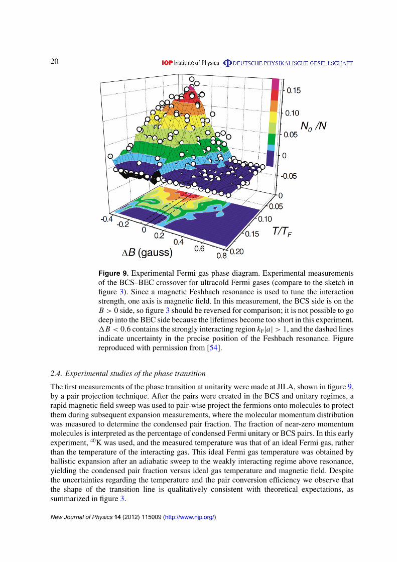
Figure 9. Experimental Fermi gas phase diagram. Experimental measurementsof the BCS–BEC crossover for ultracold Fermi gases (compare to the sketch infigure 3). Since a magnetic Feshbach resonance is used to tune the interactionstrength, one axis is magnetic field. In this measurement, the BCS side is on theB > 0 side, so figure 3 should be reversed for comparison; it is not possible to godeep into the BEC side because the lifetimes become too short in this experiment.1B < 0.6 contains the strongly interacting region kF|a|> 1, and the dashed linesindicate uncertainty in the precise position of the Feshbach resonance. Figurereproduced with permission from [54].

2.4. Experimental studies of the phase transition

The first measurements of the phase transition at unitarity were made at JILA, shown in figure 9,by a pair projection technique. After the pairs were created in the BCS and unitary regimes, arapid magnetic field sweep was used to pair-wise project the fermions onto molecules to protectthem during subsequent expansion measurements, where the molecular momentum distributionwas measured to determine the condensed pair fraction. The fraction of near-zero momentummolecules is interpreted as the percentage of condensed Fermi unitary or BCS pairs. In this earlyexperiment, 40K was used, and the measured temperature was that of an ideal Fermi gas, ratherthan the temperature of the interacting gas. This ideal Fermi gas temperature was obtained byballistic expansion after an adiabatic sweep to the weakly interacting regime above resonance,yielding the condensed pair fraction versus ideal gas temperature and magnetic field. Despitethe uncertainties regarding the temperature and the pair conversion efficiency we observe thatthe shape of the transition line is qualitatively consistent with theoretical expectations, assummarized in figure 3.

New Journal of Physics 14 (2012) 115009 (http://www.njp.org/)

21

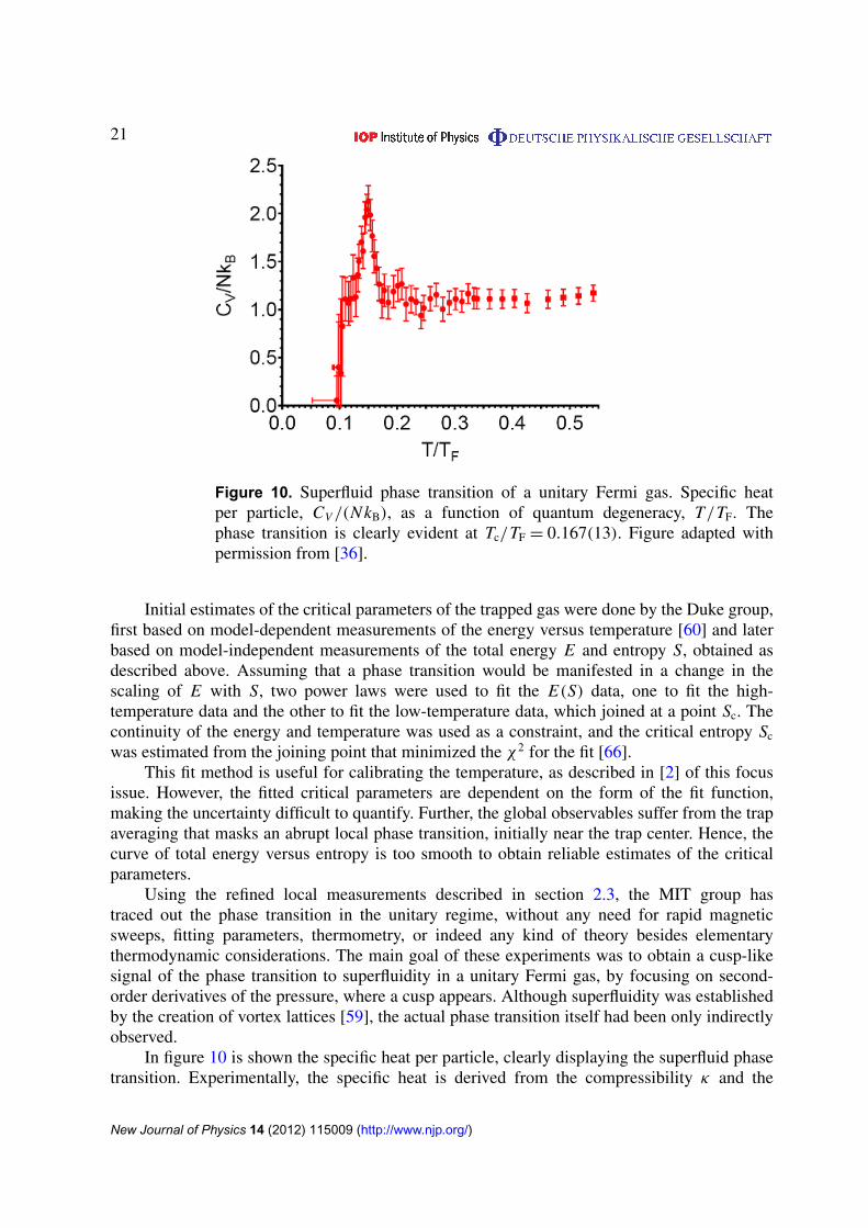
Figure 10. Superfluid phase transition of a unitary Fermi gas. Specific heatper particle, CV /(NkB), as a function of quantum degeneracy, T/TF. Thephase transition is clearly evident at Tc/TF = 0.167(13). Figure adapted withpermission from [36].

Initial estimates of the critical parameters of the trapped gas were done by the Duke group,first based on model-dependent measurements of the energy versus temperature [60] and laterbased on model-independent measurements of the total energy E and entropy S, obtained asdescribed above. Assuming that a phase transition would be manifested in a change in thescaling of E with S, two power laws were used to fit the E(S) data, one to fit the high-temperature data and the other to fit the low-temperature data, which joined at a point Sc. Thecontinuity of the energy and temperature was used as a constraint, and the critical entropy Sc

was estimated from the joining point that minimized the χ2 for the fit [66].This fit method is useful for calibrating the temperature, as described in [2] of this focus

issue. However, the fitted critical parameters are dependent on the form of the fit function,making the uncertainty difficult to quantify. Further, the global observables suffer from the trapaveraging that masks an abrupt local phase transition, initially near the trap center. Hence, thecurve of total energy versus entropy is too smooth to obtain reliable estimates of the criticalparameters.

Using the refined local measurements described in section 2.3, the MIT group hastraced out the phase transition in the unitary regime, without any need for rapid magneticsweeps, fitting parameters, thermometry, or indeed any kind of theory besides elementarythermodynamic considerations. The main goal of these experiments was to obtain a cusp-likesignal of the phase transition to superfluidity in a unitary Fermi gas, by focusing on second-order derivatives of the pressure, where a cusp appears. Although superfluidity was establishedby the creation of vortex lattices [59], the actual phase transition itself had been only indirectlyobserved.

In figure 10 is shown the specific heat per particle, clearly displaying the superfluid phasetransition. Experimentally, the specific heat is derived from the compressibility κ and the

New Journal of Physics 14 (2012) 115009 (http://www.njp.org/)

22

pressure P [36],CV

kB N=

5

2

TF

T

(p−

1

κ

), (17)

where κ = κ/κ0 and p ≡ P/P0 are normalized to the non-interacting Fermi gas compressibilityκ0 =

32

1nEF

and pressure P0 =25nEF, respectively. Using n = (∂P/∂µ)T , the compressibility

can be written as κ = (1/n2)(∂n/∂µ)T = (1/n2)(∂2 P/∂2µ)T . As κ is a second derivative ofthe pressure, the specific heat shows a clear cusp-like signature (figure 10). Qualitatively, thebehavior of CV can be understood as follows: as one approaches the phase transition fromabove, T/Tc > 1, the compressibility increases due to the attraction between fermions; belowthe phase transition, T/Tc < 1, the compressibility decreases because fermions are bound intopairs, and it becomes more difficult to squeeze the gas, i.e. to change the single-particle density.

2.5. Universal hydrodynamics and transport

Transport properties of the unitary Fermi gas are of interest for several reasons. The firstreason is related to the main theme of this review: holographic dualities suggest a newkind of universality in the transport properties of strongly interacting quantum fluids. Weexpect, in particular, that the shear viscosity to entropy density ratio is close to the valueη/s ∼ h/(4πkB) originally discovered in the QGP, and first obtained theoretically using theAdS /CFT correspondence [11], where AdS is a special maximally symmetric space–timedescribed in detail in section 4.2, and CFT stands for conformal field theory. The second reasonis that transport properties are very sensitive to the strength of the interaction, and the types ofquasiparticles present in the system. The Bertsch parameter, which characterizes the effect ofinteractions on the energy per particle, varies by about a factor of two between the weak coupling(BCS) and strong coupling (unitarity) limits. The shear viscosity, on the other hand, changesby many orders of magnitude. Finally, quantum-limited transport has also been observed insystems that are of great practical significance, in particular in the strange metal phase of high-Tc compounds; see the contribution by Guo et al to this focus issue [110].

Transport properties have been studied experimentally by exciting hydrodynamic modes,such as collective oscillations [56, 111–114], collective flow [46, 115], sound [116] androtational modes [117]. In a system that can be described in terms of quasiparticles thehydrodynamic description is valid if the Knudsen number K n = lmfp/L , the ratio of the meanfree path lmfp to the system size L , is small17. In the unitary gas the mean free path islmfp = 1/(nσ), where n is the density and σ = 4π/k2 is the universal cross section. In the high-temperature limit the thermal average cross section is σ = 4λ2

dB. The Knudsen number of aunitary gas confined in a cigar-shaped harmonic trap is

K n =3π 1/2

4(3λz N )1/3

(T

TFI

)2

, (18)

where we have taken L as the radius in the narrow or z direction. Here, N is the numberof particles, λz was defined previously as the aspect ratio of the trap and TFI is the global

17 Criteria for the validity of hydrodynamics can also be formulated if there is no underlying quasiparticledescription, a situation that is of great interest in connection with holographic dualities. In this case, hydrodynamicsis based on a gradient expansion of the conserved currents. The ratio of the O(v) to O(∂v) terms in the stress tensoris known as the Reynolds number, Re = vLmn/η. Validity of the gradient expansion requires that the Reynoldsnumber be large.

New Journal of Physics 14 (2012) 115009 (http://www.njp.org/)

23

Fermi temperature for a harmonically trapped ideal gas; see section 2.1. Using N = 2× 105 andλz = 0.045 as in [113], we conclude that hydrodynamics is expected to be valid for T <

∼ 5TFI.For the Fermi gas viscosity measurements described in this focus issue [2, 115], the maximumtemperature is T ' 1.5 TFI and K n 6 0.09.

Nearly ideal hydrodynamic behavior was first observed in the expansion of a unitary Fermigas after release from a deformed trap [46]; see figure 4. For a ballistic gas the expansion reflectsthe isotropic local momentum distribution in the trap. As a result the gas expands in all directionsand the cloud slowly becomes spherical. For a hydrodynamic system the expansion is drivenby gradients in the pressure. In the case of a deformed cloud the gradients are largest in theshort direction of the trap, and the expansion takes place mostly in the transverse direction. Asa result, the cloud eventually becomes elongated along what was originally the short direction.This phenomenon is analogous to the elliptic flow observed in heavy-ion collisions, as describedin section 3.5. What is also remarkable is the fact that even though the gas becomes more diluteas it expands, this effect is compensated for by the growth in the mean cross section. As aconsequence, the gas remains hydrodynamic throughout the expansion. Ballistic behavior setsin eventually only because of imperfections, such as the fact that the scattering length is nottruly infinite.

The role of dissipative effects, in particular shear viscosity, was first studied in collectivemodes. The radial breathing mode can be excited by removing the confining potential, lettingthe gas expand for a short period of time, and then restoring the potential. Hydrodynamicbehavior can be established by measuring the frequency of the breathing mode. For an ideal fluidω =√

10/3ω0, whereas in a ballistic system ω = 2ω0 [118, 119]. The transition from ballisticbehavior in the BCS limit to hydrodynamics in the unitary limit was observed experimentallyin [111, 112]. In the hydrodynamic regime damping is expected to be dominated by dissipativeterms in the equations of fluid dynamics. The energy dissipation is given by

E =−∫

dx{η(x)

2

(∇iv j +∇ jvi −

2

3δi j(∇ · v)

)2

+ ζ(x) (∇ · v)2 +κ(x)

T(∇T )2

}, (19)

where vi is the fluid velocity, η is the shear viscosity, ζ is the bulk viscosity, κ is the thermalconductivity, and all derivatives, divergences and gradients are spatial. At unitarity the systemis scale invariant and the bulk viscosity is expected to vanish [78, 120]. This prediction wasexperimentally checked by Cao et al [121] and Dusling and Schafer [121]. Thermal conductivityis not important because the system remains isothermal in ideal hydrodynamics. Temperaturegradients only appear due to shear viscosity, and their contribution to dissipation is higher orderin the gradient expansion. This means that damping is dominated by shear viscosity.

Collective modes in ideal fluid dynamics are described by scaling solutions of Euler’sequation. This means that the shape of the density profile does not change during the evolution,and that the velocity is linear in the coordinates. The solution is analogous to Hubble flows incosmology and the Bjorken expansion of a QGP, as discussed in section 3.5. In the case of ascaling solution, the shear stresses ∂iv j are spatially constant, and the energy dissipated onlydepends on the spatial integral of η. On dimensional grounds we can write η = hnαn. For ascale invariant system αn is only a function of the dimensionless variable n2/3h2/(mkBT ), i.e. afunction of the reduced temperature T/TF. The reduced temperature varies across the trap, butfor a given fluid element it remains approximately constant during the hydrodynamic evolutionof the system. This implies that the damping constant of a collective mode is related to the

New Journal of Physics 14 (2012) 115009 (http://www.njp.org/)

24

spatial average of the shear viscosity in the initial equilibrium state

〈αn〉 =1

N

∫dx η(x). (20)

The extracted values of 〈αn〉 can be converted into the trap averaged shear viscosity to entropydensity ratio by using the measured entropy per particle. This type of analysis was originallycarried out in [122, 123], where it was observed that η/s <∼ 0.5h/kB in the vicinity of Tc.More recently, Cao et al [115] showed that in the high-temperature regime αn exhibits thescaling behavior expected from the solution of the linearized Boltzmann equation. The shearviscosity due to elastic two-body scattering has the form η ' nplmfp, where p ∼ λ−1

dB is themean quasiparticle momentum. As we saw above, lmfp ∼ 1/(nσ)∼ 1/(nλ2

dB). This implies thatat high temperature η ∼ λ−3

dB . The coefficient of proportionality was determined by Bruun andco-workers [8] and Brun and Smith [124]. They find that

η =15

32√π

(mkBT )3/2

h2 . (21)

There is an important problem related to equation (21) that affects the extraction of theshear viscosity from experiments with scaling flows. Equation (21), which is reliable in thehigh-temperature or low-density part of the cloud, is independent of the density18. As aconsequence the integral in equation (20) diverges in the low-density region. A solution to thisproblem was proposed in [126, 127]: in the low-density regime, the viscous relaxation time τR '

η/(nkBT ), which is the time it takes for the dissipative stresses to relax to the Navier–Stokesform η(∇iv j +∇ jvi −

23δi j∇kvk), becomes very large. Since the dissipative stresses are initially

zero, taking relaxation into account suppresses the contribution from the dilute corona. Asimplified version of this approach was used in Cao et al [2, 115]. The relaxation time andits relation to the spectral function of the shear tensor are discussed in the contribution by Brabyet al [128].

The shear viscosity drops with temperature and is expected to reach a minimum near Tc. Inthis regime quantum effects are important. T -matrix calculations can be found in [129] and inthe contributions by Guo et al and LeClair in this focus issue [110, 130]. It is also possible that inthis regime quasiparticle descriptions break down completely, and the most efficient descriptionof the unitary gas near Tc is in terms of a suitable weakly coupled holographic dual. Progresstoward constructing holographic duals of non-relativistic quantum fluids is summarized insection 4.3.4.

In the low-temperature superfluid regime the appropriate description is superfluid (two-fluid) hydrodynamics [131]. Superfluid hydrodynamics predicts the existence of additionalhydrodynamic modes, in particular second sound, and contains additional transport coefficientsthat come into play if there is relative motion between the superfluid and normal components ofthe fluid. There are proposals for exciting second sound modes in the literature [132], but theseideas have not yet been confirmed. At very low temperature the shear viscosity is expected to bedominated by phonons, similar to liquid helium or dilute Bose gases. Elastic phonon scatteringgives η ∼ 1/T 5 [133], whereas inelastic processes can give a slower increase at low temperature,η ∼ 1/T [9]. These predictions are difficult to verify experimentally because the phonon freepath is quite large.

18 This is a general property of the viscosity of dilute gases, and was first noticed by Maxwell. The result wasexperimentally confirmed by Maxwell himself, who measured the damping of oscillating discs in a partiallyevacuated container [125].

New Journal of Physics 14 (2012) 115009 (http://www.njp.org/)

25

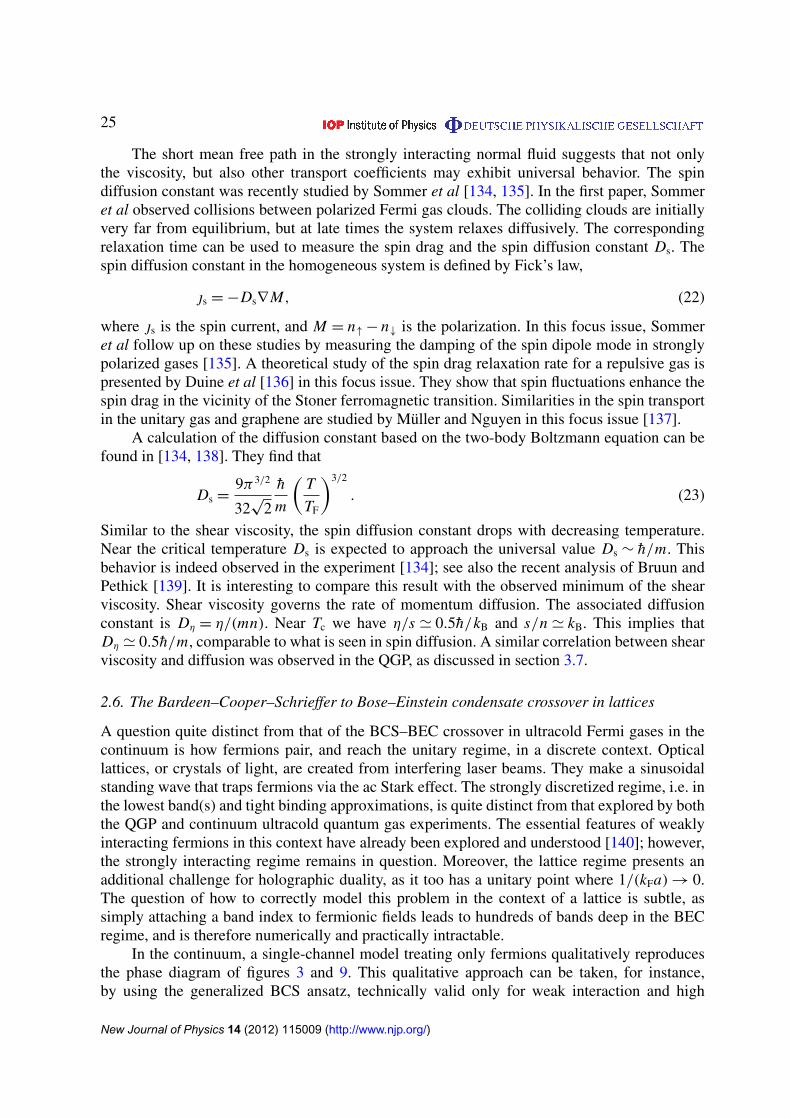
The short mean free path in the strongly interacting normal fluid suggests that not onlythe viscosity, but also other transport coefficients may exhibit universal behavior. The spindiffusion constant was recently studied by Sommer et al [134, 135]. In the first paper, Sommeret al observed collisions between polarized Fermi gas clouds. The colliding clouds are initiallyvery far from equilibrium, but at late times the system relaxes diffusively. The correspondingrelaxation time can be used to measure the spin drag and the spin diffusion constant Ds. Thespin diffusion constant in the homogeneous system is defined by Fick’s law,

s =−Ds∇M, (22)

where s is the spin current, and M = n↑− n↓ is the polarization. In this focus issue, Sommeret al follow up on these studies by measuring the damping of the spin dipole mode in stronglypolarized gases [135]. A theoretical study of the spin drag relaxation rate for a repulsive gas ispresented by Duine et al [136] in this focus issue. They show that spin fluctuations enhance thespin drag in the vicinity of the Stoner ferromagnetic transition. Similarities in the spin transportin the unitary gas and graphene are studied by Muller and Nguyen in this focus issue [137].

A calculation of the diffusion constant based on the two-body Boltzmann equation can befound in [134, 138]. They find that

Ds =9π3/2

32√

2

h

m

(T

TF

)3/2

. (23)

Similar to the shear viscosity, the spin diffusion constant drops with decreasing temperature.Near the critical temperature Ds is expected to approach the universal value Ds ∼ h/m. Thisbehavior is indeed observed in the experiment [134]; see also the recent analysis of Bruun andPethick [139]. It is interesting to compare this result with the observed minimum of the shearviscosity. Shear viscosity governs the rate of momentum diffusion. The associated diffusionconstant is Dη = η/(mn). Near Tc we have η/s ' 0.5h/kB and s/n ' kB. This implies thatDη ' 0.5h/m, comparable to what is seen in spin diffusion. A similar correlation between shearviscosity and diffusion was observed in the QGP, as discussed in section 3.7.

2.6. The Bardeen–Cooper–Schrieffer to Bose–Einstein condensate crossover in lattices

A question quite distinct from that of the BCS–BEC crossover in ultracold Fermi gases in thecontinuum is how fermions pair, and reach the unitary regime, in a discrete context. Opticallattices, or crystals of light, are created from interfering laser beams. They make a sinusoidalstanding wave that traps fermions via the ac Stark effect. The strongly discretized regime, i.e. inthe lowest band(s) and tight binding approximations, is quite distinct from that explored by boththe QGP and continuum ultracold quantum gas experiments. The essential features of weaklyinteracting fermions in this context have already been explored and understood [140]; however,the strongly interacting regime remains in question. Moreover, the lattice regime presents anadditional challenge for holographic duality, as it too has a unitary point where 1/(kFa)→ 0.The question of how to correctly model this problem in the context of a lattice is subtle, assimply attaching a band index to fermionic fields leads to hundreds of bands deep in the BECregime, and is therefore numerically and practically intractable.

In the continuum, a single-channel model treating only fermions qualitatively reproducesthe phase diagram of figures 3 and 9. This qualitative approach can be taken, for instance,by using the generalized BCS ansatz, technically valid only for weak interaction and high

New Journal of Physics 14 (2012) 115009 (http://www.njp.org/)

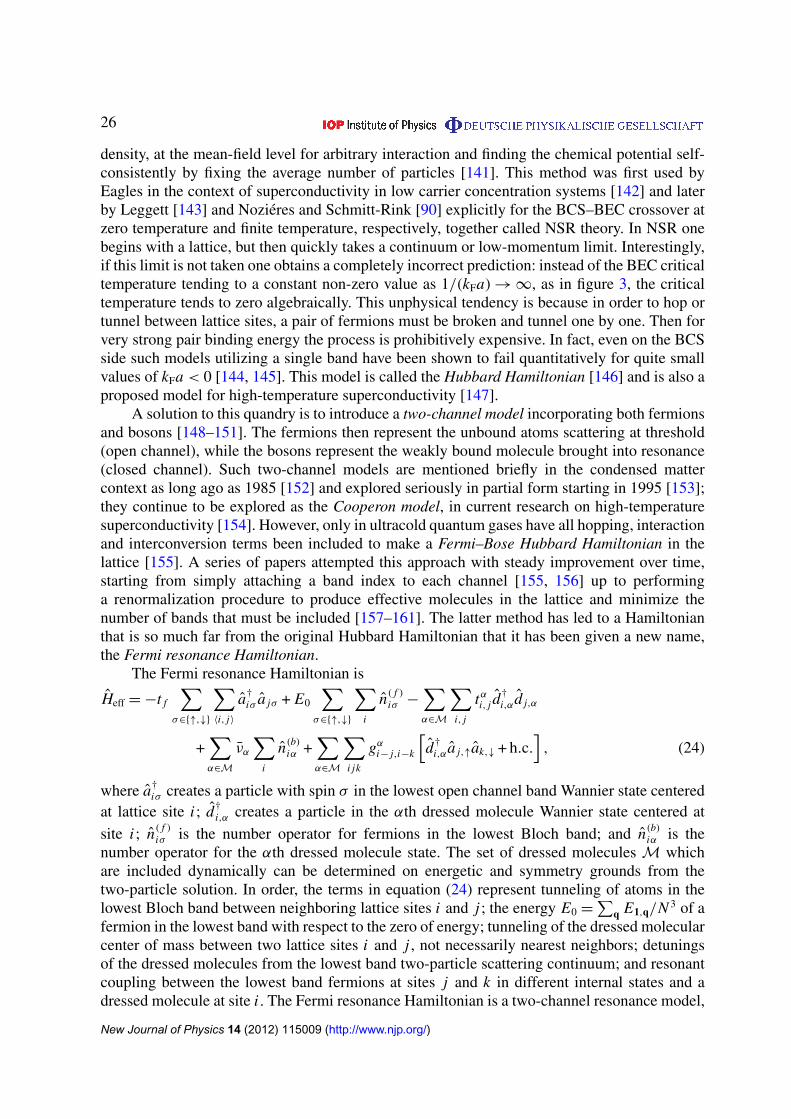
26

density, at the mean-field level for arbitrary interaction and finding the chemical potential self-consistently by fixing the average number of particles [141]. This method was first used byEagles in the context of superconductivity in low carrier concentration systems [142] and laterby Leggett [143] and Nozieres and Schmitt-Rink [90] explicitly for the BCS–BEC crossover atzero temperature and finite temperature, respectively, together called NSR theory. In NSR onebegins with a lattice, but then quickly takes a continuum or low-momentum limit. Interestingly,if this limit is not taken one obtains a completely incorrect prediction: instead of the BEC criticaltemperature tending to a constant non-zero value as 1/(kFa)→∞, as in figure 3, the criticaltemperature tends to zero algebraically. This unphysical tendency is because in order to hop ortunnel between lattice sites, a pair of fermions must be broken and tunnel one by one. Then forvery strong pair binding energy the process is prohibitively expensive. In fact, even on the BCSside such models utilizing a single band have been shown to fail quantitatively for quite smallvalues of kFa < 0 [144, 145]. This model is called the Hubbard Hamiltonian [146] and is also aproposed model for high-temperature superconductivity [147].

A solution to this quandry is to introduce a two-channel model incorporating both fermionsand bosons [148–151]. The fermions then represent the unbound atoms scattering at threshold(open channel), while the bosons represent the weakly bound molecule brought into resonance(closed channel). Such two-channel models are mentioned briefly in the condensed mattercontext as long ago as 1985 [152] and explored seriously in partial form starting in 1995 [153];they continue to be explored as the Cooperon model, in current research on high-temperaturesuperconductivity [154]. However, only in ultracold quantum gases have all hopping, interactionand interconversion terms been included to make a Fermi–Bose Hubbard Hamiltonian in thelattice [155]. A series of papers attempted this approach with steady improvement over time,starting from simply attaching a band index to each channel [155, 156] up to performinga renormalization procedure to produce effective molecules in the lattice and minimize thenumber of bands that must be included [157–161]. The latter method has led to a Hamiltonianthat is so much far from the original Hubbard Hamiltonian that it has been given a new name,the Fermi resonance Hamiltonian.

The Fermi resonance Hamiltonian is

Heff =−t f

∑σ∈{↑,↓}

∑〈i, j〉

a†iσ a jσ + E0

∑σ∈{↑,↓}

∑i

n( f )iσ −

∑α∈M

∑i, j

tαi, j d†i,αd j,α

+∑α∈M

να∑

i

n(b)iα +∑α∈M

∑i jk

gαi− j,i−k

[d†

i,αa j,↑ak,↓ + h.c.], (24)

where a†iσ creates a particle with spin σ in the lowest open channel band Wannier state centered

at lattice site i ; d†i,α creates a particle in the αth dressed molecule Wannier state centered at

site i ; n( f )iσ is the number operator for fermions in the lowest Bloch band; and n(b)iα is the

number operator for the αth dressed molecule state. The set of dressed molecules M whichare included dynamically can be determined on energetic and symmetry grounds from thetwo-particle solution. In order, the terms in equation (24) represent tunneling of atoms in thelowest Bloch band between neighboring lattice sites i and j ; the energy E0 =

∑q E1,q/N 3 of a

fermion in the lowest band with respect to the zero of energy; tunneling of the dressed molecularcenter of mass between two lattice sites i and j , not necessarily nearest neighbors; detuningsof the dressed molecules from the lowest band two-particle scattering continuum; and resonantcoupling between the lowest band fermions at sites j and k in different internal states and adressed molecule at site i . The Fermi resonance Hamiltonian is a two-channel resonance model,

New Journal of Physics 14 (2012) 115009 (http://www.njp.org/)

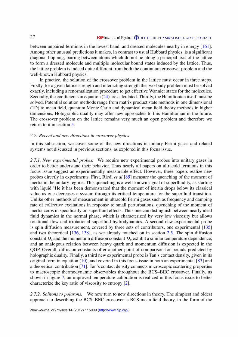
27

between unpaired fermions in the lowest band, and dressed molecules nearby in energy [161].Among other unusual predictions it makes, in contrast to usual Hubbard physics, is a significantdiagonal hopping, pairing between atoms which do not lie along a principal axis of the latticeto form a dressed molecule and multiple molecular bound states induced by the lattice. Thus,the lattice problem is indeed quite different from both the continuum crossover problem and thewell-known Hubbard physics.

In practice, the solution of the crossover problem in the lattice must occur in three steps.Firstly, for a given lattice strength and interacting strength the two-body problem must be solvedexactly, including a renormalization procedure to get effective Wannier states for the molecules.Secondly, the coefficients in equation (24) are calculated. Thirdly, the Hamiltonian itself must besolved. Potential solution methods range from matrix product state methods in one dimensional(1D) to mean field, quantum Monte Carlo and dynamical mean field theory methods in higherdimensions. Holographic duality may offer new approaches to this Hamiltonian in the future.The crossover problem on the lattice remains very much an open problem and therefore wereturn to it in section 5.

2.7. Recent and new directions in crossover physics

In this subsection, we cover some of the new directions in unitary Fermi gases and relatedsystems not discussed in previous sections, as explored in this focus issue.

2.7.1. New experimental probes. We require new experimental probes into unitary gases inorder to better understand their behavior. Thus nearly all papers on ultracold fermions in thisfocus issue suggest an experimentally measurable effect. However, three papers realize newprobes directly in experiments. First, Riedl et al [85] measure the quenching of the moment ofinertia in the unitary regime. This quenching is a well-known signal of superfluidity, as startingwith liquid 4He it has been demonstrated that the moment of inertia drops below its classicalvalue as one decreases a system through its critical temperature for the superfluid transition.Unlike other methods of measurement in ultracold Fermi gases such as frequency and dampingrate of collective excitations in response to small perturbations, quenching of the moment ofinertia zeros in specifically on superfluid effects. Thus one can distinguish between nearly idealfluid dynamics in the normal phase, which is characterized by very low viscosity but allowsrotational flow and irrotational superfluid hydrodynamics. A second new experimental probeis spin diffusion measurement, covered by three sets of contributors, one experimental [135]and two theoretical [136, 138], as we already touched on in section 2.5. The spin diffusionconstant Ds and the momentum diffusion constant Dη exhibit a similar temperature dependence,and an analogous relation between heavy quark and momentum diffusion is expected in theQGP. Overall, diffusion constants offer another point of comparison for bounds predicted byholographic duality. Finally, a third new experimental probe is Tan’s contact density, given in itsoriginal form in equation (10), and covered in this focus issue in both an experimental [83] anda theoretical contribution [71]. Tan’s contact density connects microscopic scattering propertiesto macroscopic thermodynamic observables throughout the BCS–BEC crossover. Finally, asshown in figure 7, an improved temperature calibration is realized in this focus issue to bettercharacterize the key ratio of viscosity to entropy [2].

2.7.2. Solitons to polarons. We now turn to new directions in theory. The simplest and oldestapproach to describing the BCS–BEC crossover is BCS mean field theory, in the form of the

New Journal of Physics 14 (2012) 115009 (http://www.njp.org/)

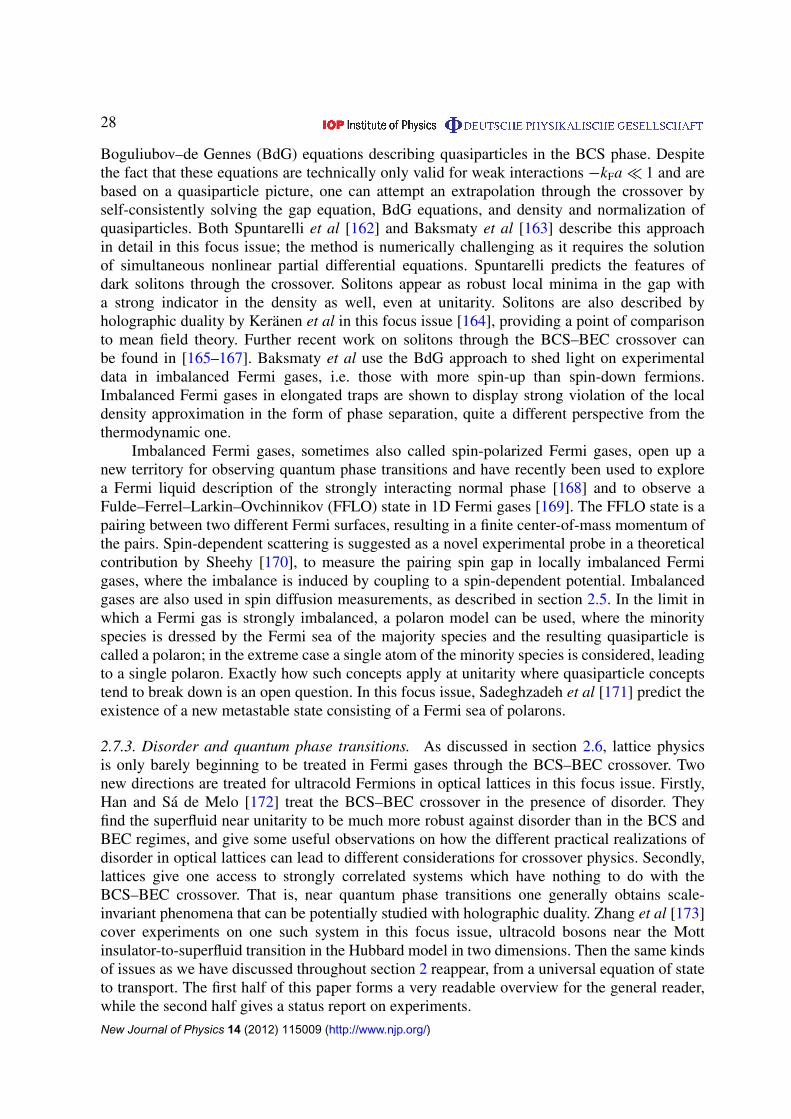
28

Boguliubov–de Gennes (BdG) equations describing quasiparticles in the BCS phase. Despitethe fact that these equations are technically only valid for weak interactions −kFa� 1 and arebased on a quasiparticle picture, one can attempt an extrapolation through the crossover byself-consistently solving the gap equation, BdG equations, and density and normalization ofquasiparticles. Both Spuntarelli et al [162] and Baksmaty et al [163] describe this approachin detail in this focus issue; the method is numerically challenging as it requires the solutionof simultaneous nonlinear partial differential equations. Spuntarelli predicts the features ofdark solitons through the crossover. Solitons appear as robust local minima in the gap witha strong indicator in the density as well, even at unitarity. Solitons are also described byholographic duality by Keranen et al in this focus issue [164], providing a point of comparisonto mean field theory. Further recent work on solitons through the BCS–BEC crossover canbe found in [165–167]. Baksmaty et al use the BdG approach to shed light on experimentaldata in imbalanced Fermi gases, i.e. those with more spin-up than spin-down fermions.Imbalanced Fermi gases in elongated traps are shown to display strong violation of the localdensity approximation in the form of phase separation, quite a different perspective from thethermodynamic one.

Imbalanced Fermi gases, sometimes also called spin-polarized Fermi gases, open up anew territory for observing quantum phase transitions and have recently been used to explorea Fermi liquid description of the strongly interacting normal phase [168] and to observe aFulde–Ferrel–Larkin–Ovchinnikov (FFLO) state in 1D Fermi gases [169]. The FFLO state is apairing between two different Fermi surfaces, resulting in a finite center-of-mass momentum ofthe pairs. Spin-dependent scattering is suggested as a novel experimental probe in a theoreticalcontribution by Sheehy [170], to measure the pairing spin gap in locally imbalanced Fermigases, where the imbalance is induced by coupling to a spin-dependent potential. Imbalancedgases are also used in spin diffusion measurements, as described in section 2.5. In the limit inwhich a Fermi gas is strongly imbalanced, a polaron model can be used, where the minorityspecies is dressed by the Fermi sea of the majority species and the resulting quasiparticle iscalled a polaron; in the extreme case a single atom of the minority species is considered, leadingto a single polaron. Exactly how such concepts apply at unitarity where quasiparticle conceptstend to break down is an open question. In this focus issue, Sadeghzadeh et al [171] predict theexistence of a new metastable state consisting of a Fermi sea of polarons.

2.7.3. Disorder and quantum phase transitions. As discussed in section 2.6, lattice physicsis only barely beginning to be treated in Fermi gases through the BCS–BEC crossover. Twonew directions are treated for ultracold Fermions in optical lattices in this focus issue. Firstly,Han and Sa de Melo [172] treat the BCS–BEC crossover in the presence of disorder. Theyfind the superfluid near unitarity to be much more robust against disorder than in the BCS andBEC regimes, and give some useful observations on how the different practical realizations ofdisorder in optical lattices can lead to different considerations for crossover physics. Secondly,lattices give one access to strongly correlated systems which have nothing to do with theBCS–BEC crossover. That is, near quantum phase transitions one generally obtains scale-invariant phenomena that can be potentially studied with holographic duality. Zhang et al [173]cover experiments on one such system in this focus issue, ultracold bosons near the Mottinsulator-to-superfluid transition in the Hubbard model in two dimensions. Then the same kindsof issues as we have discussed throughout section 2 reappear, from a universal equation of stateto transport. The first half of this paper forms a very readable overview for the general reader,while the second half gives a status report on experiments.

New Journal of Physics 14 (2012) 115009 (http://www.njp.org/)

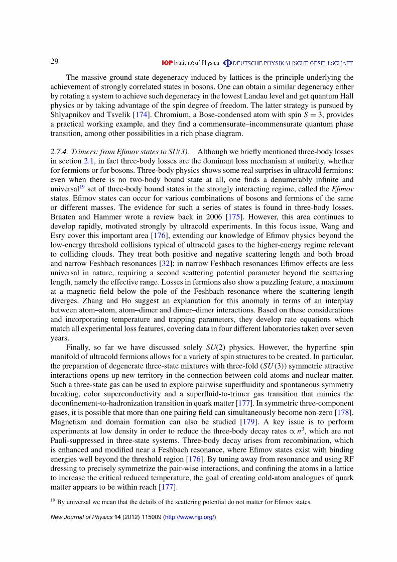
29

The massive ground state degeneracy induced by lattices is the principle underlying theachievement of strongly correlated states in bosons. One can obtain a similar degeneracy eitherby rotating a system to achieve such degeneracy in the lowest Landau level and get quantum Hallphysics or by taking advantage of the spin degree of freedom. The latter strategy is pursued byShlyapnikov and Tsvelik [174]. Chromium, a Bose-condensed atom with spin S = 3, providesa practical working example, and they find a commensurate–incommensurate quantum phasetransition, among other possibilities in a rich phase diagram.

2.7.4. Trimers: from Efimov states to SU(3). Although we briefly mentioned three-body lossesin section 2.1, in fact three-body losses are the dominant loss mechanism at unitarity, whetherfor fermions or for bosons. Three-body physics shows some real surprises in ultracold fermions:even when there is no two-body bound state at all, one finds a denumerably infinite anduniversal19 set of three-body bound states in the strongly interacting regime, called the Efimovstates. Efimov states can occur for various combinations of bosons and fermions of the sameor different masses. The evidence for such a series of states is found in three-body losses.Braaten and Hammer wrote a review back in 2006 [175]. However, this area continues todevelop rapidly, motivated strongly by ultracold experiments. In this focus issue, Wang andEsry cover this important area [176], extending our knowledge of Efimov physics beyond thelow-energy threshold collisions typical of ultracold gases to the higher-energy regime relevantto colliding clouds. They treat both positive and negative scattering length and both broadand narrow Feshbach resonances [32]: in narrow Feshbach resonances Efimov effects are lessuniversal in nature, requiring a second scattering potential parameter beyond the scatteringlength, namely the effective range. Losses in fermions also show a puzzling feature, a maximumat a magnetic field below the pole of the Feshbach resonance where the scattering lengthdiverges. Zhang and Ho suggest an explanation for this anomaly in terms of an interplaybetween atom–atom, atom–dimer and dimer–dimer interactions. Based on these considerationsand incorporating temperature and trapping parameters, they develop rate equations whichmatch all experimental loss features, covering data in four different laboratories taken over sevenyears.

Finally, so far we have discussed solely SU(2) physics. However, the hyperfine spinmanifold of ultracold fermions allows for a variety of spin structures to be created. In particular,the preparation of degenerate three-state mixtures with three-fold (SU (3)) symmetric attractiveinteractions opens up new territory in the connection between cold atoms and nuclear matter.Such a three-state gas can be used to explore pairwise superfluidity and spontaneous symmetrybreaking, color superconductivity and a superfluid-to-trimer gas transition that mimics thedeconfinement-to-hadronization transition in quark matter [177]. In symmetric three-componentgases, it is possible that more than one pairing field can simultaneously become non-zero [178].Magnetism and domain formation can also be studied [179]. A key issue is to performexperiments at low density in order to reduce the three-body decay rates ∝ n3, which are notPauli-suppressed in three-state systems. Three-body decay arises from recombination, whichis enhanced and modified near a Feshbach resonance, where Efimov states exist with bindingenergies well beyond the threshold region [176]. By tuning away from resonance and using RFdressing to precisely symmetrize the pair-wise interactions, and confining the atoms in a latticeto increase the critical reduced temperature, the goal of creating cold-atom analogues of quarkmatter appears to be within reach [177].

19 By universal we mean that the details of the scattering potential do not matter for Efimov states.

New Journal of Physics 14 (2012) 115009 (http://www.njp.org/)

30

3. Quantum chromodynamics, the quark–gluon plasma and heavy-ion collisions

In this section we will give an introduction to the physics of the QGP. This is a vast subjectand we will not attempt to provide a comprehensive review here. Recent reviews of variousissues related to quark matter and the QGP can be found in [20, 180–184] and the results ofthe experimental program at the RHIC at BNL are summarized in [185]. Some results of theLHC program at the European Organization for Nuclear Research (CERN) can be found in thecontributions [186, 187, 189] and in the recent review [190].

We will focus on observables and experimental results that are important in establishingthe presence of strong correlations in the QGP and that provide direct connections to thephysics of ultracold atomic gases and holographic dualities. In section 3.1 we introduce quantumchromodynamics (QCD), the theory of the strong interaction, and discuss the QCD phasediagram. The differences between weakly coupled QCD plasmas and strongly coupled QCDfluids are discussed in section 3.2. The experimental study of high-temperature QCD matteris based on heavy-ion collisions. We provide an overview of the experimental program insection 3.3 and discuss specific observables (multiplicities, flow, energy loss and heavy quarks)in sections 3.4–3.7. Finally, a discussion of open issues can be found in section 5.2.

3.1. Quantum chromodynamics and the phase diagram

QCD describes the behavior of strongly interacting matter, such as protons, neutrons and nucleias well as the hot and dense matter created in heavy-ion collisions, in terms of quarks and gluonsand their interactions. The complicated phenomenology of the strong interaction is encoded ina deceptively simple Lagrangian. The Lagrangian is formulated in terms of quark fields qc

α fand gluon fields Aa

µ. Here, α = 1, . . . , 4 is a Dirac spinor index (corresponding, in the Diracrepresentation, to quarks and anti-quarks with spin up and down), c = 1, . . . , Nc is a color indexand f = up, down, strange, charm, bottom, top is a flavor index. In our world the number ofcolors is Nc = 3, but as a theoretical laboratory it is useful to consider theories with Nc 6= 3.The dynamics of the theory is governed by the color degrees of freedom. The gluon field Aa

µ

is a vector field (such as the photon) labeled by an adjoint color index a = 1, . . . , 8. The octetof gluon fields can be used to construct a matrix valued field Aµ = Aa

µλa

2 , where λa is a set oftraceless, Hermitian, 3× 3 matrices. Repeated indices are assumed to be summed throughoutour treatment. The QCD Lagrangian is

L=−1

4GaµνG

aµν +

N f∑f

q f (iγµDµ−m f )q f , (25)

where Gaµν is the QCD field strength tensor:

Gaµν = ∂µAa

ν − ∂ν Aaµ + g f abc Ab

µAcν, (26)

and f abc= 4i Tr([λa, λb]λc) is a set of numbers called the SU (3) structure constants. The

covariant derivative acting on the quark fields is

iDµq =

(i∂µ + g Aa

µ

λa

2

)q, (27)

and m f is the mass of the quarks. The different terms in equation (25) describe the interactionbetween quarks and gluons, as well as nonlinear three- and four-gluon interactions. It is

New Journal of Physics 14 (2012) 115009 (http://www.njp.org/)

31

important to note that, except for the number of flavors and their masses, the structure of theQCD Lagrangian is completely fixed by a local SU (3) color symmetry.

For many purposes, we can consider the light flavors (up, down and strange) to beapproximately massless, and the heavy flavors (charm, bottom and top) to be infinitely massive.In this limit the QCD Lagrangian contains a single dimensionless parameter, the couplingconstant g. If quantum effects are taken into account the coupling becomes scale dependent.At leading order the running coupling constant is

g2(q2)=16π2

b0 log(q2/32QCD)

, b0 =11

3Nc−

2

3N f , (28)

where q is a characteristic momentum and N f is the number of active flavors (N f = 3if we consider charm, bottom and top to be infinitely heavy). The result in equation (28)implies that, as a quantum theory, QCD is not characterized by a dimensionless coupling butby a dimensionful scale, the QCD scale parameter 3QCD. This effect is called dimensionaltransmutation [191]. We also observe that the coupling decreases with increasing momentum.This is the phenomenon of asymptotic freedom [192, 193]. The flip side of asymptoticfreedom is anti-screening or confinement: the effective interaction between quarks increaseswith distance.

In massless QCD the scale parameter is an arbitrary parameter (a QCD ‘standardkilogram’), but once QCD is embedded in the standard model and quarks acquire masses byelectroweak symmetry breaking the QCD scale is fixed by the choice of units in the standardmodel. The numerical value of 3QCD depends on the renormalization scheme used to deriveequation (28). Physical masses, as well as the value of b0, are independent of this choice. Inthe modified minimal subtraction (M S), one finds that 3QCD ' 200 MeV; see the QCD sectionin [194].

Asymptotic freedom and the symmetries of QCD determine the main phases of stronglyinteracting matter that appear in the QCD phase diagram shown in figure 11. In this figurewe show the phases of QCD as a function of the temperature T and the baryon chemicalpotential µ. The chemical potential µ controls the baryon density ρ, defined as 1/3 times thenumber density of quarks minus the number density of anti-quarks.

At zero temperature and chemical potential the interaction between quarks is dominatedby large distances and the effective coupling is large. As a consequence, quarks and gluons arepermanently confined in color singlet hadrons, with masses of order 3QCD. For example, theproton has a mass of mp = 935 MeV.20

If we think of the proton as composed of three constituent quarks this implies that quarkshave effective masses m Q ' mp/3'3QCD. This should be compared to the bare up and downquark masses which are of the order of 10 MeV.

Strong interactions between quarks and anti-quarks lead to a vacuum condensate ofqq pairs, 〈qq〉 ' −33

QCD [195–197]. This vacuum condensate spontaneously breaks theapproximate chiral SU (3)L× SU (3)R flavor symmetry of the QCD Lagrangian. Chiralsymmetry breaking implies the existence of Goldstone bosons, particles with masses smallerthan 3QCD. These particles are known as pions, kaons and etas21.

20 Note that we are quoting the mass in units of energy, setting the speed of light equal to unity.21 The SU (3)L× SU (3)R is explicitly broken by quark masses and the mass of the charged pion is mπ = 139 MeV,which is not much smaller than 3QCD. The lightest non-Goldstone particle is the rho meson, which has a massmρ = 770 MeV.

New Journal of Physics 14 (2012) 115009 (http://www.njp.org/)

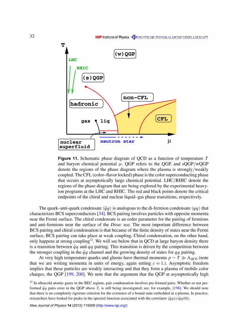
32

Figure 11. Schematic phase diagram of QCD as a function of temperature Tand baryon chemical potential µ. QGP refers to the QGP, and sQGP/wQGPdenote the regions of the phase diagram where the plasma is strongly/weaklycoupled. The CFL (color–flavor locked) phase is the color superconducting phasethat occurs at asymptotically large chemical potential. LHC/RHIC denote theregions of the phase diagram that are being explored by the experimental heavy-ion programs at the LHC and RHIC. The red and black points denote the criticalendpoints of the chiral and nuclear liquid–gas phase transitions, respectively.

The quark–anti-quark condensate 〈qq〉 is analogous to the di-fermion condensate 〈qq〉 thatcharacterizes BCS superconductors [34]. BCS pairing involves particles with opposite momentanear the Fermi surface. The chiral condensate is an order parameter for the pairing of fermionsand anti-fermions near the surface of the Dirac sea. The most important difference betweenBCS pairing and chiral condensation is that because of the finite density of states near the Fermisurface, BCS pairing can take place at weak coupling. Chiral condensation, on the other hand,only happens at strong coupling22. We will see below that in QCD at large baryon density thereis a transition between qq and qq pairing. This transition is driven by the competition betweenthe stronger coupling in the qq channel and the growing density of states for qq pairing.

At very high temperature quarks and gluons have thermal momenta p ∼ T �3QCD (notethat we are writing momenta in units of energy, again setting c = 1.). Asymptotic freedomimplies that these particles are weakly interacting and that they form a plasma of mobile colorcharges, the QGP [199, 200]. We note that the argument that the QGP at asymptotically high

22 In ultracold atomic gases in the BEC regime, pair condensation involves pre-formed pairs. Whether or not pre-formed qq pairs exist in the QGP above Tc is still being investigated; see, for example, [198]. We should notethat there is no completely rigorous criterion for the existence of a bound state embedded in a plasma. In practice,researchers have looked for peaks in the spectral function associated with the correlator 〈qq(x)qq(0)〉.

New Journal of Physics 14 (2012) 115009 (http://www.njp.org/)

33

temperature is weakly coupled is somewhat more subtle than it might appear at first sight. Iftwo particles in the plasma interact via large-angle scattering, then the momentum transfer islarge, and the effective coupling is weak because of asymptotic freedom. However, the colorCoulomb interaction is dominated by small-angle scattering, and it is not immediately clearwhy the effective interaction that governs small-angle scattering is weak. The important point isthat in a high-temperature plasma there is a large thermal population (n ∼ T 3) of mobile chargesthat screen the interaction at distances beyond the Debye length rD ∼ 1/(gT ). We also note thateven in the limit T �3QCD the QGP contains a non-perturbative sector of static magnetic colorfields [201]. This sector is strongly coupled, but it does not contribute to thermodynamic ortransport properties of the plasma in the limit T →∞.

The plasma phase exhibits neither color confinement nor chiral symmetry breaking. Thismeans that the high-temperature QGP phase must be separated from the low-temperaturehadronic phase by a phase transition. The nature of this transition is very sensitive to the valuesof the quark masses. In QCD with massless u,d and infinitely massive s,c,b,t quarks thetransition is second order [202]. In the case of massless (or sufficiently light) u,d,s quarks thetransition is first order. Lattice simulations show that for realistic quark masses, mu ' md '

10 MeV and ms ' 120 MeV, the phase transition is a rapid crossover [203]. The transitiontemperature, defined in terms of the chiral susceptibility, is Tc ' 151± 3± 3 MeV [204, 205].

The transition is believed to strengthen as a function of chemical potential, so that thereis a critical µ at which the crossover turns into a first-order phase transition [206]. This pointis the critical endpoint of the chiral phase transition. Due to the fermion sign problem it isvery difficult to locate the critical endpoint using simulations on the lattice. A number ofexploratory calculations have been performed [207–210], but at this point it is not even clearwhether the idea that the transition strengthens as the baryon chemical potential increases iscorrect [211]. The critical endpoint is interesting because it is the only point on the phasetransition line at which the correlation length diverges (there is a similar endpoint on the nuclearliquid–gas transition line). This means that the critical point may manifest itself in heavy-ioncollisions in terms of enhanced fluctuations [212]. The idea is that one can tune the baryonchemical potential by changing the collision energy, since lower beam energy allows for morestopping of the baryons in the initial state and therefore leads to higher chemical potential.As the collision energy is varied one looks for non-monotonic behavior of fluctuation andcorrelation observables. A typical observable is the variance (divided by the mean) of the netnumber of protons (protons minus anti-protons) in a finite sub-volume, 〈(1Np)

2〉/〈Np〉 with

1Np = Np−〈Np〉. A beam energy scan is now under way at RHIC, and similar scans have beenperformed at lower energy as part of the CERN fixed target program [213, 214].

At low temperature the first phase one encounters when the chemical potential is increasedfrom zero is nuclear matter, a strongly correlated superfluid composed of approximatelynon-relativistic neutrons and protons. It is interesting to note that nuclear matter in weakn↔ p + e + νe equilibrium is neutron rich23 and that the neutron–neutron scattering length24

23 Isolated neutrons are unstable with regard to the decay into protons, electrons and anti-neutrinos. If we ignorethe role of electrons, then dense matter is composed of equal numbers of protons and neutrons because thisconfiguration optimizes the total Fermi energy. Taking electrons into account we observe that for a given density ofprotons and electrons the Fermi energy of the electrons is much bigger than that of protons, and the lowest energystate is neutron rich.24 1 fm (Fermi)= 10−15 m is the typical unit of length in nuclear and particle physics. 1 fm is approximately equalto the radius of the proton and neutron.

New Journal of Physics 14 (2012) 115009 (http://www.njp.org/)

34

ann ' 20 fm is much larger than the average inter-particle spacing, rnn ' 1.9 fm at nuclear mattersaturation density. As a consequence, dilute nuclear matter is closely related to the unitaryatomic Fermi gases discussed in section 2.

At very large chemical potential, we can use arguments similar to those in the high-temperature limit to establish that quarks and gluons are weakly coupled. The main differencebetween cold quark matter and the hot QGP is that because of the large density of states nearthe quark Fermi surface even weak interactions can cause qualitative changes in the groundstate of dense matter. In particular, attractive interactions between quark pairs lead to colorsuperconductivity and the formation of a 〈qq〉 condensate. Since quarks carry color, flavor andspin labels, many superconducting phases are possible. The most symmetric of these, knownas the color–flavor locked (CFL) phase, is predicted to exist at very high density [215, 216].In the CFL phase the diquark order parameter is 〈q A

α f q Bβg〉 ∼ εαβε

ABCε f gC . This order parameterhas a number of interesting properties. It breaks the U (1) symmetry associated with baryonnumber, leading to superfluidity, and it breaks the chiral SU (3)L× SU (3)R symmetry. Exceptfor Goldstone modes the spectrum is fully gapped; fermions acquire a BCS-pairing gap, andgauge fields are screened by the Meissner effect. This implies that the CFL phase, even thoughit arises from a superdense liquid of quarks, shares many properties of superfluid nuclear matter.

The CFL phase involves equal pair condensates 〈ud〉 = 〈us〉 = 〈ds〉 of all three light quarkflavors. As the density is lowered, effects of the non-zero strange quark mass become moreimportant, and less symmetric phases are likely to appear [180]. Calculations based on weakcoupling suggest that the first non-CFL phase is a CFL-like phase with a Bose condensateof kaons, and the second phase involves a standing meson wave superimposed on the kaoncondensate [217, 218]. Other possibilities which may appear in strong coupling include a phasewith up–down pairing only (2SC), or separate spin-one condensates of up, down and strangequarks.

Some guidance an analyzing the competition between these phases may come fromstudying analogue models of the quark–hadron phase transition based on ultracold atomic gases.A number of authors have pointed out the possibility of a BCS–BEC crossover in dense quarkmatter [219]. The basic idea is that as the density is lowered, quark Cooper pairs become morestrongly bound and form a diquark Bose condensate. At lower densities one may also encountera mixture of condensed diquarks and unpaired quarks. The physics of this system can be studiedusing ultracold boson–fermion mixtures [24, 25, 220, 221]. Finally, it may be possible to studythe transition from nucleons, bound states of three quarks, to color superconducting diquarksusing three-species systems of ultracold fermions [177–179, 222].

Color superconductivity affects both the equation of state and the transport properties ofdense quark matter. These effects may manifest themselves in the structure and evolution ofneutron stars. Possible signatures of pairing appear in the mass–radius relation, the coolingcurve and the relation between the spin-down rate and the magnetic field. There are twocontributions in this focus issue that touch on these issues. Shovkovy and Wang [223]study the bulk viscosity of normal quark matter in the large-amplitude regime. Anglani etal [224] investigate the interaction of collective modes in the CFL phase. This calculationis a first step toward more accurate calculations of transport properties of the CFL phase[225, 226].

New Journal of Physics 14 (2012) 115009 (http://www.njp.org/)

35

3.2. Weakly versus strongly coupled plasmas

At asymptotically high temperature the coupling is weak and properties of the QGP can besystematically computed. One of the most basic properties is the equation of state. In thefollowing we will consider a related quantity, the entropy density. The perturbative expansionof the entropy density is [227, 228]

s = T 3{c0 + c2 g2 + c3 g3 + · · ·

}, (29)

where g is the QCD coupling constant from equation (28) and we have chosen units such thath = kB = 1. The expansion is performed with the coupling g = g(µ) evaluated at a fixed scaleµ. Higher order terms contain logarithms of the form log(2πT/µ), which combine with lowerorder terms to eliminate the dependence on the arbitrary scale µ, and lead to an expansion interms of the running coupling g(q) evaluated at a scale q ' 2πT . The first term in equation (29)corresponds to the Stefan–Boltzmann law, and c0 is proportional to the number of degrees offreedom,

c0 =2π 2

45

(2(N 2

c − 1)

+ 4Nc N f7

8

), (30)

where 2(N 2c − 1) is the number of degrees of freedom from the gluons and 4Nc N f from the

quarks. The naive perturbative expansion is an expansion in powers of g2. Odd powers ofg appear because of infrared divergences. As we approach the phase transition the couplingbecomes large and higher order terms are no longer small. Indeed, the convergence propertiesof the expansion in equation (29) are extremely poor: the series shows no signs of convergingunless the coupling is taken to be much smaller than one, g� 1, corresponding to completelyunrealistic temperatures of the order of 1 TeV. The convergence can be improved significantly byusing a self-consistent quasiparticle expansion [229]. This means that the perturbative expansionis formulated not in terms of free quarks and gluons, but in terms of quasiquarks and quasigluonswhich have effective masses and effective interactions.

Quasiparticle expansions fit lattice data quantitatively down to temperatures T ∼ 2Tc. Inthis regime s/s0 ' 0.85, where s0 is the entropy density of a non-interacting plasma. In the pastthis was frequently taken as evidence that quasiparticles are not strongly coupled at temperaturesrelevant to the early stages of heavy-ion collisions at RHIC or the LHC. A new perspective onthis question is provided by holographic duality; see section 4. Holographic duality maps thestrongly interacting quantum field theories onto one higher dimensional classical gravity, inparticular anti-de Sitter space (AdS). In the original version of the mapping, the quantum fieldtheory (QFT) is a QCD-like theory known as the N = 4 supersymmetric (SUSY) Yang–Millstheory [230]. This theory is conformal. This means that its coupling constant does not run,g2(q2)= const, and there is no analogue of 3QCD. It also does not have a phase transition, andso the theory is in the plasma phase for all values of the coupling. The particle content of theN = 4 SUSY Yang–Mills theory differs from that of QCD. The theory has no quarks, and inaddition to gluons it contains supersymmetric fermionic partners of gluons called gluinos aswell as additional colored scalar fields. Nevertheless, the plasma phase shares many features ofthe QGP, and by focusing on a ratio such as s/s0 we can remove the difference in the number ofdegrees of freedom. Later versions of holographic duality relax conformal and supersymmetricrequirements, but still do not map precisely onto QCD.

Using holographic duality it was found that in the limit of strong coupling and a largenumber of colors the entropy density of the SUSY Yang–Mills theory is s/s0 = 0.75 [231].

New Journal of Physics 14 (2012) 115009 (http://www.njp.org/)

36

This value is remarkably close to the result observed in lattice QCD calculations near thephase transition, casting doubt on an interpretation of the data in terms of weakly coupledquasiparticles. More generally, holographic duality demonstrates that thermodynamic propertiesof the plasma need not be very sensitive to the strength of the interaction.

Holographic duality also shows that, in contrast to equilibrium properties, transportproperties of the plasma are very sensitive probes of the strength of the interaction. Inperturbative QCD the shear viscosity of three-flavor QCD is [6, 232, 233]

η =kT 3

g4 log(µ∗/mD), (31)

where k = 106.67, µ∗ = 2.96T and mD ∼ gT is the screening mass. Shear viscosity is relatedto the rate of momentum diffusion. A simple estimate of the shear viscosity is [234]

η '1

3np lmfp '

1

3

p

σT, (32)

where n is the density, p is the mean momentum, lmfp is the mean free path and σT is thetransport cross section. In a perturbative QCD plasma the typical momentum is p ∼ T , andthe transport cross section is σT ∼ g4log(g)T−2. The time scale for momentum diffusion isη/(sT )∼ 1/(g4 log(g)T ). We note that in the weak coupling limit this number is parametricallylarge. In a QGP at T = 200 MeV, just above the phase transition, we have T−1

' 1 fm/c andη/s ' 9.2/g4. A typical value of the coupling is g ' 2 (corresponding to αs ' 0.3), whichimplies that η/(sT )' 0.6 fm/c.

The strong coupling limit of η/s in the SUSY Yang–Mills plasma was studied by Policastroet al [235]. They find that

η

s=

1

4π

(1 + O

(λ−3/2

)), (33)

where λ= g2 Nc is the ’t Hooft coupling. This result implies that at strong coupling momentumequilibration is almost an order of magnitude more rapid than it is in weak coupling. The ratioη/s is also close to a bound that was argued to arise from the uncertainty relation [234]. Theidea is that, because of quantum mechanics, the product p lmfp in equation (32) cannot becomesmaller than Planck’s constant h (note that we are using units in which h = 1). This impliesthat η/s <∼

13(

ns )' 0.09, where we have used the entropy per particle of a free gas [234]. The

uncertainty argument has never been made precise, since the mean free path estimate is notvalid at strong coupling. However, the holographic duality calculation was discovered to bequite general. It was shown that the strong coupling limit of η/s is universal in a large class oftheories that have gravitational duals, and that the O(λ−3/2) corrections are positive [236, 237].These observations led KSS to make the conjecture that

η

s>

1

4π(34)

is a universal bound [11] that applies to all fluids. The status of this conjecture is discussedin more detail in section 4 and sketched in figure 2. There are some known counterexamplesinvolving theories with gravitational duals described by higher derivative gravity. However, itseems clear that equation (34) applies to a large class of theories that include generalizations ofQCD.

New Journal of Physics 14 (2012) 115009 (http://www.njp.org/)

37

Experiments on collective flow in heavy-ion collisions at RHIC and the LHC (discussed insection 3.4) indicate that the viscosity of the QGP near the critical temperature is indeed close tothe proposed bound and that equilibration must be very rapid. Together with the observation ofa large energy loss of highly energetic probes of the plasma, these results led to the conclusionthat the QGP produced at RHIC must be strongly coupled [185, 238].

In the case of the SUSY Yang–Mills plasma, one can show that strong coupling impliesthe absence of well-defined quasiparticles. This can be seen most clearly by studying thespectral function ρ(ω) of the stress tensor correlation function. Kubo’s formula relates thevalue of the spectral function at zero energy to the shear viscosity. The spectral function atfinite energy carries information about the physical excitations that contribute to momentumrelaxation. In weak coupling the spectral function has a peak at zero energy. The width ofthe peak, 0 ∼ g4log(g)T , is related to the quasiparticle lifetime. The spectral function in thestrong coupling limit was computed in [239, 240]. It was found that the spectral densityis completely featureless: the intercept at zero energy smoothly connects to the continuumcontribution ρ(ω)∼ ω4.

In the case of the QGP, the evidence regarding the existence of quasiparticles isambiguous. The stress tensor correlation function in lattice QCD was studied by Meyer [4].The reconstructed spectral function is smooth, but the resolution was not sufficient to excludethe presence of quasiparticles. There are a number of results that have been interpreted asfavoring the existence of quasiparticles. One is the fact that lattice calculations of fluctuations ofconserved charges, such as baryon number and strangeness, are compatible with the behavior ofa free gas, even near Tc [241]. An experimental observation that has been cited as evidencefor the presence of quasiparticles is the approximate quark-number scaling of the ellipticflow parameter v2 [242]. Another experimental observable that may shed some light on thequasiparticle structure is the heavy quark diffusion constant D, which we will discuss insection 3.7. The main observation is that kinetic theory and holographic duality make verydifferent predictions about the relation between the momentum relaxation time η/(sT ) and theheavy quark relaxation time m Q D/T [181].

3.3. Nuclear collisions: initial conditions

The experimental study of heavy-ion collisions at relativistic energies, which were long seen asthe best environments for the production of the QGP, began in the late 1980s with fixed targetprograms both at CERN near Geneva, and at BNL, outside of New York City; see [243–245]for historical overviews. These two programs were essential in building up a vital experimentalcommunity, formed of larger and larger collaborations as the experiments became more andmore sophisticated. The programs at CERN and BNL demonstrated that heavy-ion collisionsproduce strongly interacting, approximately equilibrated matter. The next step was taken withthe turn-on of the RHIC at Brookhaven in 2000, which brought heavy-ion physics into thecollider era, with accessibility to processes calculatable with perturbative QCD. Colliders areaccelerators with counter-circulating beams in which the entire collision energy is available forparticle production. RHIC collides gold ions with a beam energy such that every nucleon ineach of the beams has an energy of 100 GeV. Since the rest mass energy of a nucleon is about1 GeV, this implies a relativistic γ factor of about 100. When two bunches of counter-rotating

New Journal of Physics 14 (2012) 115009 (http://www.njp.org/)

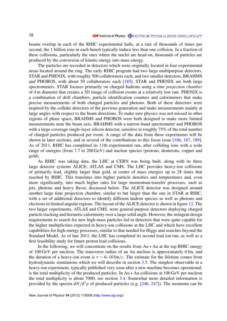
38

beams overlap in each of the RHIC experimental halls, at a rate of thousands of times persecond, the 1 billion ions in each bunch typically induce less than one collision. In a fraction ofthese collisions, particularly the ones where the nuclei are head-on, thousands of particles areproduced by the conversion of kinetic energy into mass energy.

The particles are recorded in detectors which were originally located in four experimentalareas located around the ring. The early RHIC program had two large multipurpose detectors,STAR and PHENIX, with roughly 500 collaborators each, and two smaller detectors, BRAHMSand PHOBOS, with about 50 collaborators each [185]. STAR and PHENIX are both largespectrometers. STAR focuses primarily on charged hadrons using a time projection chamberof 4 m diameter that creates a 3D image of collision events at a relatively low rate. PHENIX isa combination of drift chambers, particle identification counters and calorimeters that makeprecise measurements of both charged particles and photons. Both of these detectors wereinspired by the collider detectors of the previous generation and make measurements mainly atlarge angles with respect to the beam directions. To make sure physics was not missed in otherregions of phase space, BRAHMS and PHOBOS were both designed to make more limitedmeasurements near the beam axis, BRAHMS with a narrow-band spectrometer and PHOBOSwith a large-coverage single-layer silicon detector, sensitive to roughly 75% of the total numberof charged particles produced per event. A range of the data from these experiments will beshown in later sections, and in several of the contributions to this focus issue [186, 187, 189].As of 2011, RHIC has completed its 11th experimental run, after colliding ions with a widerange of energies (from 7.7 to 200 GeV) and nuclear species (protons, deuterons, copper andgold).

As RHIC was taking data, the LHC at CERN was being built, along with its threelarge detector systems ALICE, ATLAS and CMS. The LHC provides heavy-ion collisionsof primarily lead, slightly larger than gold, at center of mass energies up to 28 times thatreached by RHIC. This translates into higher particle densities and temperatures and, evenmore significantly, into much higher rates for large momentum-transfer processes, such asjets, photons and heavy flavor, discussed below. The ALICE detector was designed aroundanother large time projection chamber, similar to but larger than the one in STAR at RHIC,with a set of additional detectors to identify different hadron species as well as photons andelectrons in limited angular regions. The layout of the ALICE detector is shown in figure 12. Thetwo larger experiments, ATLAS and CMS, were general-purpose detectors deploying chargedparticle tracking and hermetic calorimetry over a large solid angle. However, the stringent designrequirements to search for new high-mass particles led to detectors that were quite capable forthe higher multiplicities expected in heavy-ion collisions at the LHC and which have excellentcapabilities for high-energy processes, similar to that needed for Higgs and searches beyond theStandard Model. As of late 2011, the LHC has completed its second lead ion run, as well as afirst feasibility study for future proton lead collisions.

In the following, we will concentrate on the results from Au + Au at the top RHIC energyof 100 GeV per nucleon. The transverse radius of an Au nucleus is approximately 6 fm, andthe duration of a heavy-ion event is τ ∼ 6–10 fm/c. The estimate for the lifetime comes fromhydrodynamic simulations which we will describe in section 3.5. The simplest observable in aheavy-ion experiment, typically published very soon after a new machine becomes operational,is the total multiplicity of the produced particles. In Au + Au collisions at 100 GeV per nucleonthe total multiplicity is about 7000; see section 3.4. Somewhat more detailed information isprovided by the spectra dN/d3 p of produced particles (e.g. [246, 247]). The momenta can be

New Journal of Physics 14 (2012) 115009 (http://www.njp.org/)

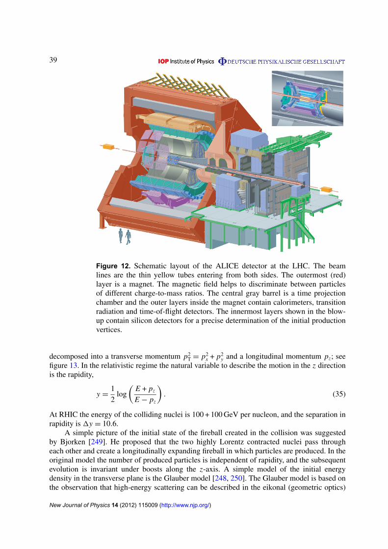
39

Figure 12. Schematic layout of the ALICE detector at the LHC. The beamlines are the thin yellow tubes entering from both sides. The outermost (red)layer is a magnet. The magnetic field helps to discriminate between particlesof different charge-to-mass ratios. The central gray barrel is a time projectionchamber and the outer layers inside the magnet contain calorimeters, transitionradiation and time-of-flight detectors. The innermost layers shown in the blow-up contain silicon detectors for a precise determination of the initial productionvertices.

decomposed into a transverse momentum p2T = p2

x + p2y and a longitudinal momentum pz; see

figure 13. In the relativistic regime the natural variable to describe the motion in the z directionis the rapidity,

y =1

2log

(E + pz

E − pz

). (35)

At RHIC the energy of the colliding nuclei is 100 + 100 GeV per nucleon, and the separation inrapidity is 1y = 10.6.

A simple picture of the initial state of the fireball created in the collision was suggestedby Bjorken [249]. He proposed that the two highly Lorentz contracted nuclei pass througheach other and create a longitudinally expanding fireball in which particles are produced. In theoriginal model the number of produced particles is independent of rapidity, and the subsequentevolution is invariant under boosts along the z-axis. A simple model of the initial energydensity in the transverse plane is the Glauber model [248, 250]. The Glauber model is based onthe observation that high-energy scattering can be described in the eikonal (geometric optics)

New Journal of Physics 14 (2012) 115009 (http://www.njp.org/)

40

Figure 13. Geometry of a high-energy heavy-ion collision. Left: collision of twoLorentz contracted gold nuclei. The beam direction is the z-axis. Right: the samecollision in the transverse plane. The impact parameter is along the x-axis, andthe remaining transverse direction is the y-axis.

approximation. The initial entropy density in the transverse plane is

s(x⊥, b)∝ TA(x⊥ + b/2)[1− exp(−σNN TA(x⊥−b/2))

]+ TA(x⊥−b/2)

[1− exp(−σNN TA(x⊥ + b/2))

], (36)

where b is the impact parameter,

TA(x⊥)=∫

dz ρA(x) (37)

is the thickness function, x≡ (x, y, z) and x⊥ ≡ (x, y), and σNN(√

s) is the nucleon–nucleoncross section. We also define the nuclear density as ρA(x). The idea behind the Glauber modelis that the initial entropy density is proportional to the number of nucleons per unit area whichexperience an inelastic collision, which we call the number of participants, Npart. Other variantsexist. For instance, one can distribute the energy density according to the number of binarynucleon–nucleon collisions, Ncoll; see [251] for a comparison. A more sophisticated theory ofthe initial energy density is provided by the color glass condensate [252, 253]. This model leadsto somewhat steeper initial transverse energy density distributions.

It should also be noted that the simple Glauber model is typically not used by moderncalculations, since it does not account for the large fluctuations which are currently attributedto the event-wise variations in the nucleon configuration coming from each nucleus and thecollision process itself. Figure 14 illustrates this by means of a single event simulated by aGlauber Monte Carlo code, which counts participants and collisions by means of a simpleprescription that collisions occur when two nucleons are within d <

√σNN/π , where σNN is the

total nucleon–nucleon inelastic cross section [248].

New Journal of Physics 14 (2012) 115009 (http://www.njp.org/)

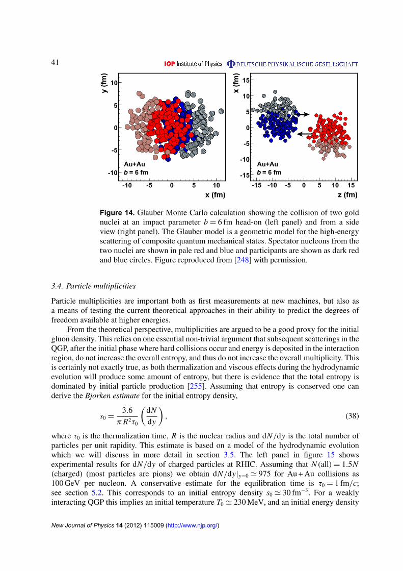
41

x (fm)-10 -5 0 5 10

y (f

m)

-10

-5

0

5

10

Au+Au

z (fm)-15 -10 -5 0 5 10 15

x (f

m)

-15

-10

-5

0

5

10

15

b = 6 fmAu+Aub = 6 fm

Figure 14. Glauber Monte Carlo calculation showing the collision of two goldnuclei at an impact parameter b = 6 fm head-on (left panel) and from a sideview (right panel). The Glauber model is a geometric model for the high-energyscattering of composite quantum mechanical states. Spectator nucleons from thetwo nuclei are shown in pale red and blue and participants are shown as dark redand blue circles. Figure reproduced from [248] with permission.

3.4. Particle multiplicities

Particle multiplicities are important both as first measurements at new machines, but also asa means of testing the current theoretical approaches in their ability to predict the degrees offreedom available at higher energies.

From the theoretical perspective, multiplicities are argued to be a good proxy for the initialgluon density. This relies on one essential non-trivial argument that subsequent scatterings in theQGP, after the initial phase where hard collisions occur and energy is deposited in the interactionregion, do not increase the overall entropy, and thus do not increase the overall multiplicity. Thisis certainly not exactly true, as both thermalization and viscous effects during the hydrodynamicevolution will produce some amount of entropy, but there is evidence that the total entropy isdominated by initial particle production [255]. Assuming that entropy is conserved one canderive the Bjorken estimate for the initial entropy density,

s0 =3.6

πR2τ0

(dN

dy

), (38)

where τ0 is the thermalization time, R is the nuclear radius and dN/dy is the total number ofparticles per unit rapidity. This estimate is based on a model of the hydrodynamic evolutionwhich we will discuss in more detail in section 3.5. The left panel in figure 15 showsexperimental results for dN/dy of charged particles at RHIC. Assuming that N (all)= 1.5N(charged) (most particles are pions) we obtain dN/dy|y=0 ' 975 for Au + Au collisions as100 GeV per nucleon. A conservative estimate for the equilibration time is τ0 = 1 fm/c;see section 5.2. This corresponds to an initial entropy density s0 ' 30 fm−3. For a weaklyinteracting QGP this implies an initial temperature T0 ' 230 MeV, and an initial energy density

New Journal of Physics 14 (2012) 115009 (http://www.njp.org/)

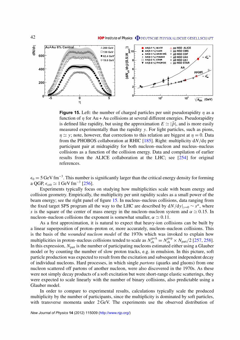
42

η-5 0 5

ηd

N/d

0

200

400

600

200 GeV

130 GeV

62.4 GeV

19.6 GeV

Au+Au 6% Central

Figure 15. Left: the number of charged particles per unit pseudorapidity η as afunction of η for Au + Au collisions at several different energies. Pseudorapidityis defined like rapidity, but using the approximation E ' |Ep|, and is more easilymeasured experimentally than the rapidity y. For light particles, such as pions,η ' y; note, however, that corrections to this relation are biggest at η = 0. Datafrom the PHOBOS collaboration at RHIC [185]. Right: multiplicity dN/dη perparticipant pair at midrapidity for both nucleon–nucleon and nucleus–nucleuscollisions as a function of the collision energy. Data and compilation of earlierresults from the ALICE collaboration at the LHC; see [254] for originalreferences.

ε0 = 5 GeV fm−3. This number is significantly larger than the critical energy density for forminga QGP, εcrit ' 1 GeV fm−3 [256].

Experiments typically focus on studying how multiplicities scale with beam energy andcollision geometry. Empirically, the multiplicity per unit rapidity scales as a small power of thebeam energy; see the right panel of figure 15. In nucleus–nucleus collisions, data ranging fromthe fixed target SPS program all the way to the LHC are described by dN/dy|y=0 ∼ sα, wheres is the square of the center of mass energy in the nucleon–nucleon system and α ' 0.15. Innucleon–nucleon collisions the exponent is somewhat smaller, α ' 0.11.

As a first approximation, it is natural to expect that heavy-ion collisions can be built bya linear superposition of proton–proton or, more accurately, nucleon–nucleon collisions. Thisis the basis of the wounded nucleon model of the 1970s which was invoked to explain howmultiplicities in proton–nucleus collisions tended to scale as N p+A

ch = N p+pch × Npart/2 [257, 258].

In this expression, Npart is the number of participating nucleons estimated either using a Glaubermodel or by counting the number of slow proton tracks, e.g. in emulsion. In this picture, softparticle production was expected to result from the excitation and subsequent independent decayof individual nucleons. Hard processes, in which single partons (quarks and gluons) from onenucleon scattered off partons of another nucleon, were also discovered in the 1970s. As thesewere not simply decay products of a soft excitation but were short-range elastic scatterings, theywere expected to scale linearly with the number of binary collisions, also predictable using aGlauber model.

In order to compare to experimental results, calculations typically scale the producedmultiplicity by the number of participants, since the multiplicity is dominated by soft particles,with transverse momenta under 2 GeV. The experiments use the observed distribution of

New Journal of Physics 14 (2012) 115009 (http://www.njp.org/)

43

multiplicities at a fixed beam energy to estimate the centrality of each collision, usuallyexpressed as a percentage of the total inelastic cross section. The 10% highest multiplicity eventsare the 0–10% centrality bin, the next highest are the 10–20% and so on. These bins are thencompared to the events with the 10% smallest impact parameter, or 10% highest multiplicityevents, in either a simple Glauber model or one which includes some model of the experimentalfluctuations [248].

The first comparisons of theory and experiment at RHIC using the multiplicity in themost central events were surprising. While many models predicted a combination of soft andsemi-hard physics processes, it was the models that were predominantly composed of softprocesses which came closest to the experimental data. This included particularly models basedon parton saturation, which were preferred by the early data. The situation is a bit different atthe LHC, as described briefly in the contribution by Steinberg [186]. At the higher energies,models which include a combination of hard and soft processes seem to do better at predictingthe multiplicities in the most central collisions. However, the centrality dependence, i.e. therelationship between the number of measured charged particles and the number of participatingnucleons (or effective nucleon–nucleon collisions), is essentially the same at RHIC and theLHC [259]. At present it is not clear how to reconcile this observation with the apparent increasein the fraction of bulk particle production stemming from hard processes.

3.5. Hydrodynamic flow

The particle density measured by the early experiments is not only valuable to comparewith different production models. It is also an essential empirical input that can be used todetermine the initial conditions for hydrodynamical models of the subsequent evolution. Thehydrodynamic description is valid if the system is in local thermal equilibrium and if thethermodynamic variables are varying smoothly. If the system has a kinetic description in termsof quasiparticles this implies that the ratio of the mean free path over the characteristic lengthscale of the system, known as the Knudsen number, must be small. There is evidence that thiscondition is satisfied during the early stages of the evolution, but it must eventually break downduring the late, dilute, stage of the evolution, since the mean free path increases with diluteness.The time when the mean free path becomes larger than the system size, more precisely, theexpansion time multiplied by the mean velocity, is called freezeout.

There are several experimental observations that provide evidence for the assumptionthat heavy-ion collisions create a thermalized state. The first observation is that the overallabundances of produced particles, including very rare ones, is described by a simple thermalmodel that contains only two parameters, the freezeout temperature T and the baryon chemicalpotential µ [183]. The second observation is that for momenta less than about 2 GeV the spectradN/d3 p of produced particles follow a Boltzmann distribution characterized by the freezeouttemperature and a collective radial expansion velocity [182]. This radial flow is clearly seenfrom the fact that the spectra of heavy particles, which receive a larger momentum boost fromthe collective velocity field, have a larger apparent temperature than the spectra of light particles.

The third piece of evidence in support of not only thermalization, but early thermalization,which means equilibration significantly before freezeout, is the observation of strong azimuthalanisotropies, typically called elliptic flow, in non-central heavy-ion collisions. Elliptic flowrepresents the collective response of the system to pressure gradients in the initial state. Theanalogous phenomenon in ultracold atomic gases is discussed in section 2.1. At finite impactparameter the initial state has the shape of an ellipse, with the short axis along the x-direction,

New Journal of Physics 14 (2012) 115009 (http://www.njp.org/)

44

and the long axis along the y-direction; see figure 13. This implies that pressure gradientsalong the x-axis are larger than along the y-axis. Hydrodynamic evolution converts the initialpressure gradients into velocity gradients in the final state. Elliptic flow is sensitive to earlythermalization because the initial anisotropy that drives elliptic flow disappears with time.Elliptic flow is quantified in terms of the second Fourier coefficient v2 of the particle distributionin the transverse plane,

p0dN

d3 p

∣∣∣∣pz=0

= v0(pT)(1 + 2v1(pT) cos(φ)+ 2v2(pT) cos(2φ)+ · · ·), (39)

where φ is the angle between the momentum vector and the x-axis. Odd Fourier momentssuch as v1 and v3 arise mainly from fluctuations in the initial state [260, 261]. Techniques formeasuring v2 and systematic trends in the results are described in some detail in the contributionby Snellings [187]. Snellings emphasizes that measurements of v2 constrain the equation of stateand the transport properties of the QGP. A similar conclusion is reached in the contribution ofLisa et al [188] to this focus issue. These authors focus on direct measurements of the shape ofthe final state using HBT (Hanbury–Brown–Twiss) interferometry.

In this section we will explain how elliptic flow can be used to constrain the ratioη/s introduced in section 3.2. In a relativistic fluid the equations of energy and momentumconservation can be written as a single equation

∂µT µν= 0, (40)

where T µν is the energy momentum tensor. In ideal fluid dynamics the form of Tµν is completelyfixed by the Lorentz invariance,

T µν= (ε + P)uµuν + Pηµν, (41)

where uµ is the fluid velocity (u2=−1) and ηµν = diag(−1, 1, 1, 1) is the metric tensor. The

hydrodynamic equations have to be supplemented by an equation of state P = P(ε). The fourequations given in equation (40) can be split into longitudinal and transverse componentsrelative to the fluid velocity. The longitudinal equation is equivalent to entropy conservation

∂µ(suµ)= 0, (42)

and the transverse equation is the relativistic Euler equation

Duµ =−1

ε + P∇⊥

µ P, (43)

where D = uµ∂µ and ∇⊥µ = ∂µ− uµD. We observe that the inertia of a relativistic fluid isgoverned by ε + P . In the non-relativistic limit we can have uµ ' (1, Ev) and ε + P ' ρ (energydensity is dominated by rest mass energy). We also find that D ' ∂t + v · ∂ and E∇⊥ ' E∂ . Theseapproximations led to the usual Euler equation. We also note that ∇⊥µ P = c2

s∇⊥

µ ε, where cs isthe speed of sound. This implies that for a given initial energy density gradient the resultingacceleration is determined by the speed of sound. Ideal fluid dynamics corresponds to the limitthat variations in the hydrodynamic variables occur on scales much larger than the mean freepath. Dissipation arises from the leading gradient terms in the energy momentum tensor. In the

New Journal of Physics 14 (2012) 115009 (http://www.njp.org/)

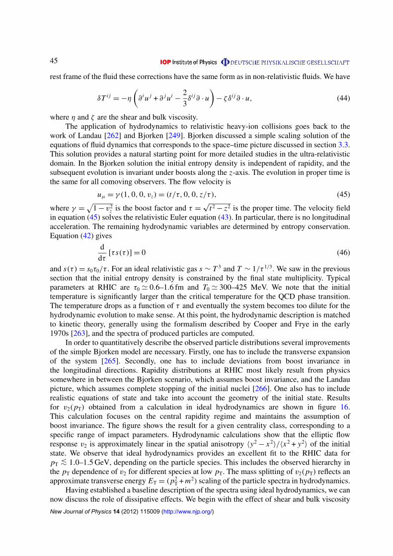
45

rest frame of the fluid these corrections have the same form as in non-relativistic fluids. We have

δT i j=−η

(∂ i u j + ∂ j ui

−2

3δi j∂ · u

)− ζ δi j∂ · u, (44)

where η and ζ are the shear and bulk viscosity.The application of hydrodynamics to relativistic heavy-ion collisions goes back to the

work of Landau [262] and Bjorken [249]. Bjorken discussed a simple scaling solution of theequations of fluid dynamics that corresponds to the space–time picture discussed in section 3.3.This solution provides a natural starting point for more detailed studies in the ultra-relativisticdomain. In the Bjorken solution the initial entropy density is independent of rapidity, and thesubsequent evolution is invariant under boosts along the z-axis. The evolution in proper time isthe same for all comoving observers. The flow velocity is

uµ = γ (1, 0, 0, vz)= (t/τ, 0, 0, z/τ), (45)

where γ =√

1− v2z is the boost factor and τ =

√t2− z2 is the proper time. The velocity field

in equation (45) solves the relativistic Euler equation (43). In particular, there is no longitudinalacceleration. The remaining hydrodynamic variables are determined by entropy conservation.Equation (42) gives

d

dτ[τ s(τ )]= 0 (46)

and s(τ )= s0τ0/τ . For an ideal relativistic gas s ∼ T 3 and T ∼ 1/τ 1/3. We saw in the previoussection that the initial entropy density is constrained by the final state multiplicity. Typicalparameters at RHIC are τ0 ' 0.6–1.6 fm and T0 ' 300–425 MeV. We note that the initialtemperature is significantly larger than the critical temperature for the QCD phase transition.The temperature drops as a function of τ and eventually the system becomes too dilute for thehydrodynamic evolution to make sense. At this point, the hydrodynamic description is matchedto kinetic theory, generally using the formalism described by Cooper and Frye in the early1970s [263], and the spectra of produced particles are computed.

In order to quantitatively describe the observed particle distributions several improvementsof the simple Bjorken model are necessary. Firstly, one has to include the transverse expansionof the system [265]. Secondly, one has to include deviations from boost invariance inthe longitudinal directions. Rapidity distributions at RHIC most likely result from physicssomewhere in between the Bjorken scenario, which assumes boost invariance, and the Landaupicture, which assumes complete stopping of the initial nuclei [266]. One also has to includerealistic equations of state and take into account the geometry of the initial state. Resultsfor v2(pT) obtained from a calculation in ideal hydrodynamics are shown in figure 16.This calculation focuses on the central rapidity regime and maintains the assumption ofboost invariance. The figure shows the result for a given centrality class, corresponding to aspecific range of impact parameters. Hydrodynamic calculations show that the elliptic flowresponse v2 is approximately linear in the spatial anisotropy 〈y2

− x2〉/〈x2 + y2

〉 of the initialstate. We observe that ideal hydrodynamics provides an excellent fit to the RHIC data forpT<∼ 1.0–1.5 GeV, depending on the particle species. This includes the observed hierarchy in

the pT dependence of v2 for different species at low pT. The mass splitting of v2(pT) reflects anapproximate transverse energy ET = (p2

T + m2) scaling of the particle spectra in hydrodynamics.Having established a baseline description of the spectra using ideal hydrodynamics, we can

now discuss the role of dissipative effects. We begin with the effect of shear and bulk viscosity

New Journal of Physics 14 (2012) 115009 (http://www.njp.org/)

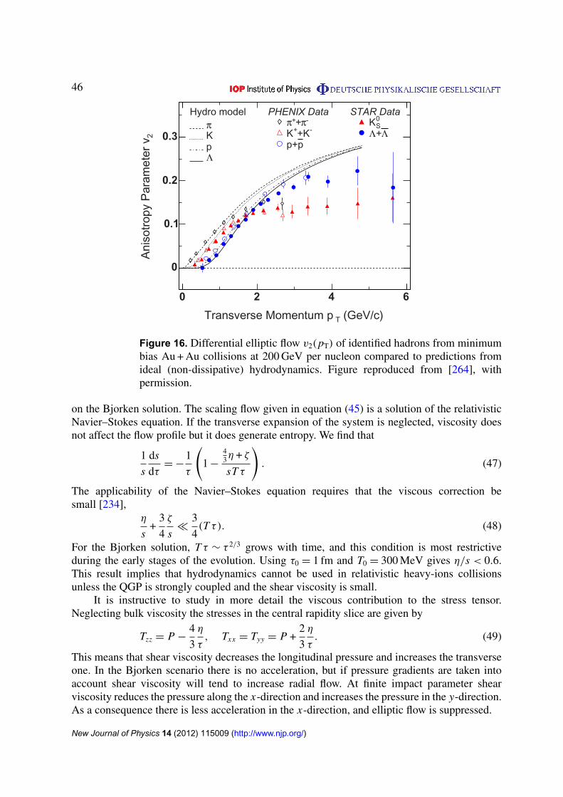
46

2A

niso

trop

y P

aram

eter

v

(GeV/c)TTransverse Momentum p

0 2 4 6

0

0.1

0.2

0.3

-π++π 0SK

-+K+Kpp+

Λ+Λ

STAR DataPHENIX DataHydro modelπKpΛ

Figure 16. Differential elliptic flow v2(pT) of identified hadrons from minimumbias Au + Au collisions at 200 GeV per nucleon compared to predictions fromideal (non-dissipative) hydrodynamics. Figure reproduced from [264], withpermission.

on the Bjorken solution. The scaling flow given in equation (45) is a solution of the relativisticNavier–Stokes equation. If the transverse expansion of the system is neglected, viscosity doesnot affect the flow profile but it does generate entropy. We find that

1

s

ds

dτ=−

1

τ

(1−

43η + ζ

sT τ

). (47)

The applicability of the Navier–Stokes equation requires that the viscous correction besmall [234],

η

s+

3

4

ζ

s�

3

4(T τ). (48)

For the Bjorken solution, T τ ∼ τ 2/3 grows with time, and this condition is most restrictiveduring the early stages of the evolution. Using τ0 = 1 fm and T0 = 300 MeV gives η/s < 0.6.This result implies that hydrodynamics cannot be used in relativistic heavy-ions collisionsunless the QGP is strongly coupled and the shear viscosity is small.

It is instructive to study in more detail the viscous contribution to the stress tensor.Neglecting bulk viscosity the stresses in the central rapidity slice are given by

Tzz = P −4

3

η

τ, Txx = Tyy = P +

2

3

η

τ. (49)

This means that shear viscosity decreases the longitudinal pressure and increases the transverseone. In the Bjorken scenario there is no acceleration, but if pressure gradients are taken intoaccount shear viscosity will tend to increase radial flow. At finite impact parameter shearviscosity reduces the pressure along the x-direction and increases the pressure in the y-direction.As a consequence there is less acceleration in the x-direction, and elliptic flow is suppressed.

New Journal of Physics 14 (2012) 115009 (http://www.njp.org/)

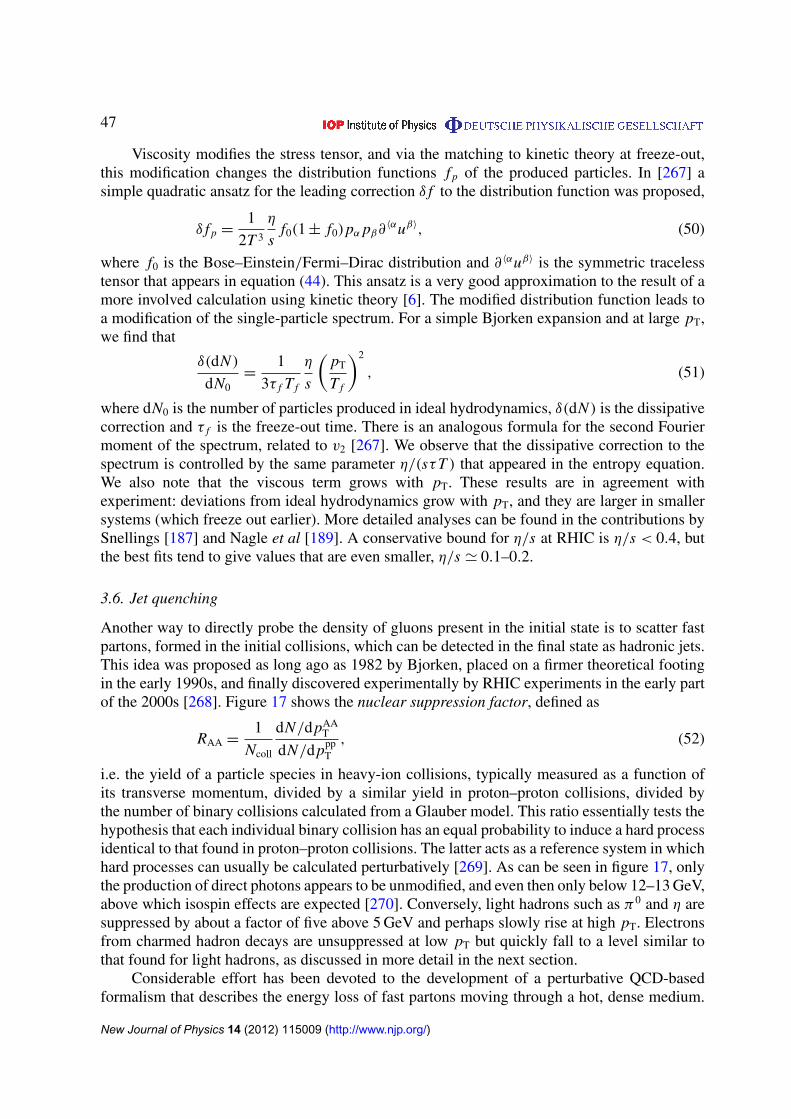
47

Viscosity modifies the stress tensor, and via the matching to kinetic theory at freeze-out,this modification changes the distribution functions f p of the produced particles. In [267] asimple quadratic ansatz for the leading correction δ f to the distribution function was proposed,

δ f p =1

2T 3

η

sf0(1± f0)pα pβ∂

〈αuβ〉, (50)

where f0 is the Bose–Einstein/Fermi–Dirac distribution and ∂ 〈αuβ〉 is the symmetric tracelesstensor that appears in equation (44). This ansatz is a very good approximation to the result of amore involved calculation using kinetic theory [6]. The modified distribution function leads toa modification of the single-particle spectrum. For a simple Bjorken expansion and at large pT,we find that

δ(dN )

dN0=

1

3τ f T f

η

s

(pT

T f

)2

, (51)

where dN0 is the number of particles produced in ideal hydrodynamics, δ(dN ) is the dissipativecorrection and τ f is the freeze-out time. There is an analogous formula for the second Fouriermoment of the spectrum, related to v2 [267]. We observe that the dissipative correction to thespectrum is controlled by the same parameter η/(sτT ) that appeared in the entropy equation.We also note that the viscous term grows with pT. These results are in agreement withexperiment: deviations from ideal hydrodynamics grow with pT, and they are larger in smallersystems (which freeze out earlier). More detailed analyses can be found in the contributions bySnellings [187] and Nagle et al [189]. A conservative bound for η/s at RHIC is η/s < 0.4, butthe best fits tend to give values that are even smaller, η/s ' 0.1–0.2.

3.6. Jet quenching

Another way to directly probe the density of gluons present in the initial state is to scatter fastpartons, formed in the initial collisions, which can be detected in the final state as hadronic jets.This idea was proposed as long ago as 1982 by Bjorken, placed on a firmer theoretical footingin the early 1990s, and finally discovered experimentally by RHIC experiments in the early partof the 2000s [268]. Figure 17 shows the nuclear suppression factor, defined as

RAA =1

Ncoll

dN/dpAAT

dN/dpppT

, (52)

i.e. the yield of a particle species in heavy-ion collisions, typically measured as a function ofits transverse momentum, divided by a similar yield in proton–proton collisions, divided bythe number of binary collisions calculated from a Glauber model. This ratio essentially tests thehypothesis that each individual binary collision has an equal probability to induce a hard processidentical to that found in proton–proton collisions. The latter acts as a reference system in whichhard processes can usually be calculated perturbatively [269]. As can be seen in figure 17, onlythe production of direct photons appears to be unmodified, and even then only below 12–13 GeV,above which isospin effects are expected [270]. Conversely, light hadrons such as π 0 and η aresuppressed by about a factor of five above 5 GeV and perhaps slowly rise at high pT. Electronsfrom charmed hadron decays are unsuppressed at low pT but quickly fall to a level similar tothat found for light hadrons, as discussed in more detail in the next section.

Considerable effort has been devoted to the development of a perturbative QCD-basedformalism that describes the energy loss of fast partons moving through a hot, dense medium.

New Journal of Physics 14 (2012) 115009 (http://www.njp.org/)

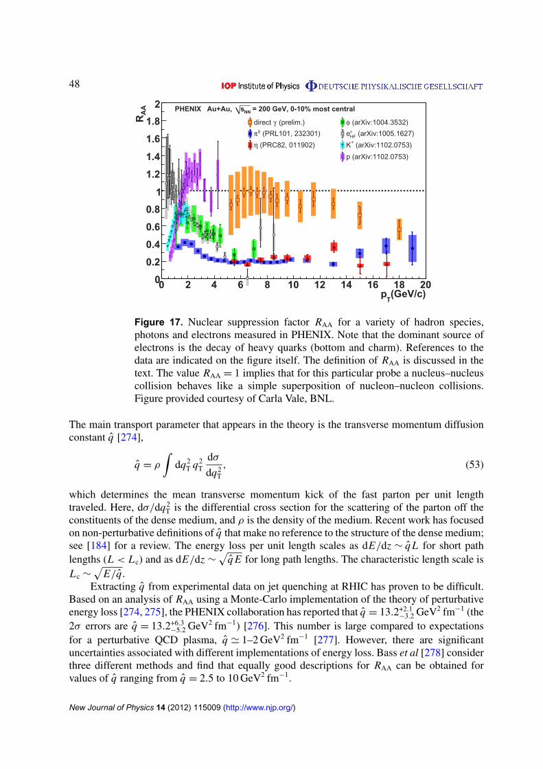
48

(GeV/c)T

p0 2 4 6 8 10 12 14 16 18 20

A

A R

0

0.2

0.4

0.6

0.8

1

1.2

1.4

1.6

1.8

2 = 200 GeV, 0-10% most centralNNsPHENIX Au+Au,

(prelim.)γdirect

(PRL101, 232301)0π (PRC82, 011902)η

(arXiv:1004.3532)φ (arXiv:1005.1627)HF

±e

(arXiv:1102.0753)+K

p (arXiv:1102.0753)

Figure 17. Nuclear suppression factor RAA for a variety of hadron species,photons and electrons measured in PHENIX. Note that the dominant source ofelectrons is the decay of heavy quarks (bottom and charm). References to thedata are indicated on the figure itself. The definition of RAA is discussed in thetext. The value RAA = 1 implies that for this particular probe a nucleus–nucleuscollision behaves like a simple superposition of nucleon–nucleon collisions.Figure provided courtesy of Carla Vale, BNL.

The main transport parameter that appears in the theory is the transverse momentum diffusionconstant q [274],

q = ρ∫

dq2T q2

T

dσ

dq2T

, (53)

which determines the mean transverse momentum kick of the fast parton per unit lengthtraveled. Here, dσ/dq2

T is the differential cross section for the scattering of the parton off theconstituents of the dense medium, and ρ is the density of the medium. Recent work has focusedon non-perturbative definitions of q that make no reference to the structure of the dense medium;see [184] for a review. The energy loss per unit length scales as dE/dz ∼ q L for short pathlengths (L < Lc) and as dE/dz ∼

√q E for long path lengths. The characteristic length scale is

Lc ∼√

E/q.Extracting q from experimental data on jet quenching at RHIC has proven to be difficult.

Based on an analysis of RAA using a Monte-Carlo implementation of the theory of perturbativeenergy loss [274, 275], the PHENIX collaboration has reported that q = 13.2+2.1

−3.2 GeV2 fm−1 (the2σ errors are q = 13.2+6.3

−5.2 GeV2 fm−1) [276]. This number is large compared to expectationsfor a perturbative QCD plasma, q ' 1–2 GeV2 fm−1 [277]. However, there are significantuncertainties associated with different implementations of energy loss. Bass et al [278] considerthree different methods and find that equally good descriptions for RAA can be obtained forvalues of q ranging from q = 2.5 to 10 GeV2 fm−1.

New Journal of Physics 14 (2012) 115009 (http://www.njp.org/)

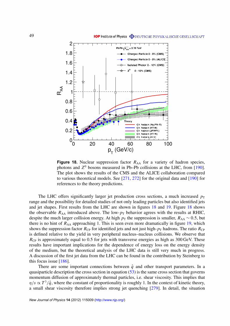
49

Figure 18. Nuclear suppression factor RAA for a variety of hadron species,photons and Z 0 bosons measured in Pb–Pb collisions at the LHC, from [190].The plot shows the results of the CMS and the ALICE collaboration comparedto various theoretical models. See [271, 272] for the original data and [190] forreferences to the theory predictions.

The LHC offers significantly larger jet production cross sections, a much increased pT

range and the possibility for detailed studies of not only leading particles but also identified jetsand jet shapes. First results from the LHC are shown in figures 18 and 19. Figure 18 showsthe observable RAA introduced above. The low-pT behavior agrees with the results at RHIC,despite the much larger collision energy. At high pT the suppression is smaller, RAA ∼ 0.5, butthere is no hint of RAA approaching 1. This is seen even more dramatically in figure 19, whichshows the suppression factor RCP for identified jets and not just high-pT hadrons. The ratio RCP

is defined relative to the yield in very peripheral nucleus–nucleus collisions. We observe thatRCP is approximately equal to 0.5 for jets with transverse energies as high as 300 GeV. Theseresults have important implications for the dependence of energy loss on the energy densityof the medium, but the theoretical analysis of the LHC data is still very much in progress.A discussion of the first jet data from the LHC can be found in the contribution by Steinberg tothis focus issue [186].

There are some important connections between q and other transport parameters. In aquasiparticle description the cross section in equation (53) is the same cross section that governsmomentum diffusion of approximately thermal particles, i.e. shear viscosity. This implies thatη/s ∝ T 3/q, where the constant of proportionality is roughly 1. In the context of kinetic theory,a small shear viscosity therefore implies strong jet quenching [279]. In detail, the situation

New Journal of Physics 14 (2012) 115009 (http://www.njp.org/)

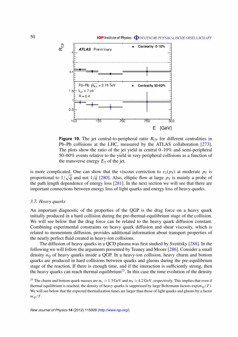
50

Figure 19. The jet central-to-peripheral ratio RCP for different centralities inPb–Pb collisions at the LHC, measured by the ATLAS collaboration [273].The plots show the ratio of the jet yield in central 0–10% and semi-peripheral50–60% events relative to the yield in very peripheral collisions as a function ofthe transverse energy ET of the jet.

is more complicated. One can show that the viscous correction to v2(pT) at moderate pT isproportional to 1/

√q and not 1/q [280]. Also, elliptic flow at large pT is mainly a probe of

the path length dependence of energy loss [281]. In the next section we will see that there areimportant connections between energy loss of light quarks and energy loss of heavy quarks.

3.7. Heavy quarks

An important diagnostic of the properties of the QGP is the drag force on a heavy quarkinitially produced in a hard collision during the pre-thermal-equilibrium stage of the collision.We will see below that the drag force can be related to the heavy quark diffusion constant.Combining experimental constraints on heavy quark diffusion and shear viscosity, which isrelated to momentum diffusion, provides additional information about transport properties ofthe nearly perfect fluid created in heavy-ion collisions.

The diffusion of heavy quarks in a QCD plasma was first studied by Svetitsky [288]. In thefollowing we will follow the arguments presented by Teaney and Moore [286]. Consider a smalldensity nQ of heavy quarks inside a QGP. In a heavy-ion collision, heavy charm and bottomquarks are produced in hard collisions between quarks and gluons during the pre-equilibriumstage of the reaction. If there is enough time, and if the interaction is sufficiently strong, thenthe heavy quarks can reach thermal equilibrium25. In this case the time evolution of the density

25 The charm and bottom quark masses are mc ' 1.3 GeV and mb ' 4.2 GeV, respectively. This implies that even ifthermal equilibrium is reached, the density of heavy quarks is suppressed by large Boltzmann factors exp(m Q/T ).We will see below that the expected thermalization times are larger than those of light quarks and gluons by a factorm Q/T .

New Journal of Physics 14 (2012) 115009 (http://www.njp.org/)

51

can be described by a diffusion equation

∂nQ

∂t= D∇

2nQ, (54)

where D is the diffusion constant. We can relate D to the drag force on the quark by using astochastic (Langevin) equation:

dpdt=−ηDp + ξ(t), 〈ξi(t)ξ j(t

′)〉 = κδi jδ(t − t ′). (55)

Here, p is the momentum of the particle, ηD is the drag coefficient and ξ(t) is a stochasticforce. In a kinetic theory picture, the stochastic force models collisions with quarks and gluonsin the plasma. The coefficient κ is related to the mean square momentum change per unittime, 3κ = 〈(1p)2〉/(1t). The Langevin equation can be integrated to determine the meansquared momentum. In the long time limit (t � η−1

D ) the particle thermalizes and we expectthat 〈p 2

〉 = 3mT . This requirement leads to the Einstein relation

ηD =κ

2mT. (56)

The relation between ηD and the diffusion constant can be determined from the mean squaredisplacement. At late times 〈[1x(t)]2

〉 = 6D|t | and

D =T

mηD=

2T 2

κ. (57)

The diffusion constant for heavy quarks in a QGP can be determined by computing the meansquare momentum transfer per unit time. At weak coupling and for approximately thermalheavy quarks, the diffusion constant is dominated by heavy quark scattering on light quarks andgluons, q Q→ q Q and gQ→ gQ. These processes are similar to the processes that determinethe shear viscosity, except that heavy quarks move slowly and the interaction only involves thecolor Coulomb interactions, whereas shear viscosity is sensitive to both electric and magneticinteractions. The leading order result in QCD with three light flavors is [286, 288]

D =6π

g4T log(2T/mD). (58)

Comparing this result with equation (31), we observe that heavy quark and momentum diffusionare related to each other. In the relevant range of coupling constants and keeping terms beyondthe leading logarithm, one finds that DT ' 6(η/s). We note that the heavy quark relaxation timeη−1

D contains an extra factor m Q/T compared to the hydrodynamic relaxation time η/(sT ). Forcharm quarks at T = 200 MeV this factor is mc/T ' 7. This implies that even if hydrodynamicbehavior is reached very quickly, η/(sT )∼ 0.2 fm, charm quarks have barely enough time toequilibrate, mc D/T ∼ 8 fm.

This simple relation between DT and η/s is broken in the strong coupling limit of theSUSY Yang–Mills plasma. Using holographic duality, one finds that [289–291]

D =2

πT

1√λ. (59)

This result implies that in the strong coupling limit there is no bound on the diffusion constantand that even very heavy quarks can possibly equilibrate. It is not clear how λ should be chosen

New Journal of Physics 14 (2012) 115009 (http://www.njp.org/)

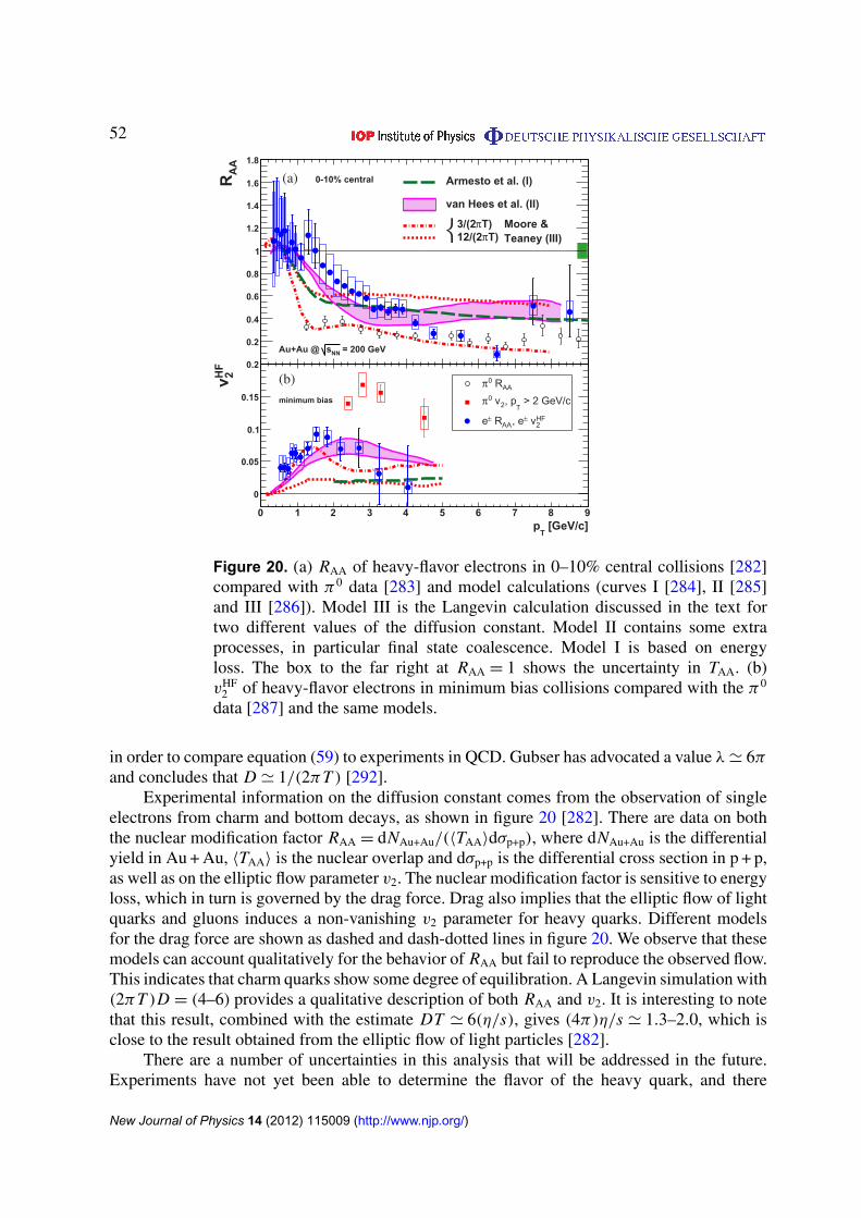
52

AA

R

0.2

0.4

0.6

0.8

1

1.2

1.4

1.6

1.8

= 200 GeVNNsAu+Au @

0-10% central(a)

Moore &Teaney (III)⎨ T)π3/(2

T)π12/(2

van Hees et al. (II)

Armesto et al. (I)

[GeV/c]T

p0 1 2 3 4 5 6 7 8 9

HF

2v

0

0.05

0.1

0.15

0.2

(b)minimum bias

AA R0π

> 2 GeV/cT

, p2 v0πHF2 v±, eAA R±e

Figure 20. (a) RAA of heavy-flavor electrons in 0–10% central collisions [282]compared with π0 data [283] and model calculations (curves I [284], II [285]and III [286]). Model III is the Langevin calculation discussed in the text fortwo different values of the diffusion constant. Model II contains some extraprocesses, in particular final state coalescence. Model I is based on energyloss. The box to the far right at RAA = 1 shows the uncertainty in TAA. (b)vHF

2 of heavy-flavor electrons in minimum bias collisions compared with the π 0

data [287] and the same models.

in order to compare equation (59) to experiments in QCD. Gubser has advocated a value λ' 6πand concludes that D ' 1/(2πT ) [292].

Experimental information on the diffusion constant comes from the observation of singleelectrons from charm and bottom decays, as shown in figure 20 [282]. There are data on boththe nuclear modification factor RAA = dNAu+Au/(〈TAA〉dσp+p), where dNAu+Au is the differentialyield in Au + Au, 〈TAA〉 is the nuclear overlap and dσp+p is the differential cross section in p + p,as well as on the elliptic flow parameter v2. The nuclear modification factor is sensitive to energyloss, which in turn is governed by the drag force. Drag also implies that the elliptic flow of lightquarks and gluons induces a non-vanishing v2 parameter for heavy quarks. Different modelsfor the drag force are shown as dashed and dash-dotted lines in figure 20. We observe that thesemodels can account qualitatively for the behavior of RAA but fail to reproduce the observed flow.This indicates that charm quarks show some degree of equilibration. A Langevin simulation with(2πT )D = (4–6) provides a qualitative description of both RAA and v2. It is interesting to notethat this result, combined with the estimate DT ' 6(η/s), gives (4π)η/s ' 1.3–2.0, which isclose to the result obtained from the elliptic flow of light particles [282].

There are a number of uncertainties in this analysis that will be addressed in the future.Experiments have not yet been able to determine the flavor of the heavy quark, and there

New Journal of Physics 14 (2012) 115009 (http://www.njp.org/)

53

are significant theoretical uncertainties in predictions of the charm and bottom spectra. Futureexperiments will be able to identify the flavor of the heavy quark. Two contributions in thisfocus issue address transport properties of heavy quarks. Meyer [293] presents a lattice studyof the Euclidean chromo-electric field correlation function. This correlation function is relatedby a Kubo formula to the diffusion constant. Rapp and Riek [294] perform a non-perturbativeT -matrix analysis of the charm quark diffusion constant and the charmonium spectral function.These and other studies, together with ongoing efforts to measure the spectra of identified heavyquarks, will shed light on the relation between the different transport properties of the plasmasuch as diffusion, energy loss and shear viscosity and help to characterize the degree to whichthe initial state in a heavy-ion collision thermalizes.

4. Holographic duality

Holography is a duality relating QFT and gravity. Roughly speaking, holographic duality mapsthe quantum physics of strongly correlated many-body systems to the classical dynamics ofblack hole horizons in one higher dimension, replacing quasiparticles with geometry as thesalient degrees of freedom. As such, holography is very much in the tradition of emergentcritical phenomena: when the system is strongly coupled, new weakly coupled degrees offreedom dynamically emerge. The novelty is that the emergent fields live in a dynamicalspace–time with an extra spatial dimension. This extra dimension plays the role of an energyscale in the QFT, with motion along the extra dimension representing a change of scale, orrenormalization group (RG) flow, in the QFT. Holography thus translates problems in quantummany-body physics, such as thermodynamics and transport physics, into equivalent problems inclassical gravity.

The power of this reorganization is that various phenomena which are easy to see, orperhaps even universal, in one presentation may be very surprising in the dual presentation,but just as universal. For example, it is a classic result that the physics of black hole horizonsin general relativity (GR) is largely independent of the details of the black hole [295–299], withsmall fluctuations of the horizon obeying the equations of viscous hydrodynamics [300]. Thedissipation of waves in this fluid encodes the absorption of energy by the black hole, with theshear viscosity taking a universal value determined by basic properties of the Einstein–Hilbertaction [300, 301]. Holographically, this is a remarkable fact: it tells us that any genericstrongly interacting quantum many-body system at finite temperature and density and with asufficiently large number of degrees of freedom per unit volume (necessary for the applicationof holographic duality) can be expected to behave, at low energies, like a nearly perfect liquidand not like a gas of long-lived quasiparticles as one might naively imagine.

More generally, holography gives us an entirely new way to define quantum field theories.Explicitly, holography provides a recipe [302–304] for using classical gravity in (d + 1)dimensions to compute quantum amplitudes that manifestly satisfy the consistency conditionsof a d-dimensional QFT (locality, causality, etc)26. In general, we do not know how to identifythe corresponding QFT in terms of more familiar tools, for example by specifying a Hamiltoniangoverning the interactions of a set of well-defined quasiparticles. Moreover, as we shall explorein some detail below, the holographic description is generally reliable precisely in situations

26 This recipe is colloquially referred to as the holographic dictionary, a sketch of which is presented in table 1.

New Journal of Physics 14 (2012) 115009 (http://www.njp.org/)

54

where most traditional techniques are not: when λ, the typical coupling in the QFT, is strong,λ� 1, and when N , the number of degrees of freedom per unit volume, is large, N � 1.27

In such cases we can simply take the gravitational description as a constructive definition ofthe QFT. Such holographic QFTs thus define a special subset of the space of well-definedQFTs which does not depend on any quasiparticle picture or conventional perturbation theory.Importantly, some of the most theoretically and experimentally interesting real-world systemsmanifestly do not have any well-defined quasiparticles upon which to base a standard QFT.Holography thus provides an entirely new way to construct consistent models of these stronglycorrelated quantum many-body systems, replacing quasiparticles with geometry as the centralorganizing principle.

An important corollary is that it is typically more fruitful to use holographic QFTs aswindows on a general class of phenomena, or to study general concepts in the space of QFTs,than to try to exactly reproduce or solve a specific QFT of previous interest. Indeed, building‘the holographic dual’ of one’s favorite QFT is generally quixotic, as the regimes of validityof holographic QFTs typically exclude the theories of previous interest. The classic exampleis SU (N ) gauge theory: QCD is given by N = 3, while the holographic dual is classical onlywhen N � 1 and weakly coupled only when the ’t Hooft coupling is also large, λ� 1. It isthus futile to try to reproduce QCD exactly. Where holography has proven useful, rather, is instudying general properties of SU (N ) gauge theories at high temperature and densities wheremany interesting phenomena arise which appear to be relatively insensitive to the precise valueof N . For example, holographic models suggest that any strongly coupled QGP should behavelike a liquid whose viscosity is very low and relatively insensitive to the precise value of thecoupling, in sharp contrast to the large viscosity and strong coupling dependence predicted byweakly coupled QCD. The low viscosity of the QGP observed at RHIC (see section 3.5) thussuggests that the RHIC fireball is indeed an extremely strongly coupled quantum liquid.

To be sure, the simplest holographic models are in many ways very different from QCD—inthe most well-understood example there are no quarks and no mass gap! What is remarkablefrom this point of view is that many of the striking features of the simplest holographicmodels persist even after the inclusion of quarks, a mass gap and other phenomenologicallyimportant ingredients. For example, in more realistic holographic models of QCD which containfundamental quarks and display confinement, the physics at low energy is again governed byhydrodynamics with an exceptionally low and coupling-insensitive viscosity. Such holographicmodels may thus be treated of as computationally tractable toy models which exhibit a richset of behaviors analogous to those observed in the laboratory, the study of which can revealqualitative, and sometimes even quantitative, general properties of the larger class of stronglycoupled QFTs.

It is important to stress that while the original discovery of holographic duality [302]required esoteric tools such as supersymmetry and conformal invariance28, the duality itself

27 More generally, holographic duality relates QFT in d-dimensions to quantum gravity in (d + 1) dimensions, withthe gravitational description becoming classical when the QFT is strongly coupled, as discussed in section 4.2.3.We will focus on regimes where the QFT is strongly coupled and the gravitational dual classical, but we emphasizethat holography remains true even when quantum gravitational (string theoretic) effects become important.28 Indeed, holographic duality is often referred to as the AdS-CFT correspondence and also as gauge–gravityduality, among many other names.

New Journal of Physics 14 (2012) 115009 (http://www.njp.org/)

55

does not depend on supersymmetry or conformality29. In fact, most current work on holographicduality involves non-supersymmetric, non-conformal QFTs. Indeed, we now have a long list ofexamples in which each of these constraints is weakened or removed (see, e.g., [305–308] andreferences therein). To date there is no example of a violation of a sharp holographic duality.From the current point of view, holographic duality is simply a true, if as yet unproven, factabout quantum field theories and quantum gravity.

While our understanding of the duality remains in various ways incomplete, holographicmodel building has already generated novel insights, including predictions for the anomalouslylow viscosity of cold atom gases, which follow from the same universal horizon physicsas that of strongly coupled SU (N ) plasmas, and lessons about jet quenching and rapidthermalization in the RHIC fireball [184]. Beyond providing new tools with which to modelspecific phenomena, holography has sometimes suggested new organizing principles forstrongly quantum dynamics, as seen, for example, in semi-holographic models of non-Fermiliquids [309–311], or in the application of classical numerical relativity to study far-from-equilibrium dynamics in extreme quantum liquids [312].

The goal of this section is to provide a brief introduction to the basic structure ofholography, first heuristically and then more precisely, as well as its origins and a few of itsapplications. We will also review a few major themes in the holographic study of extremequantum matter and give a broad, if selective view of some of the key open questions in the field.Of necessity, we omit many important topics and references. For a more detailed introduction,several excellent reviews are available, including [20, 184, 310, 313–321], from which we havedrawn heavily in preparing various parts of this section.

4.1. Why should holography be true? Two heuristic pictures

Why should a QFT in d-dimensions have anything to do with gravity in d + 1, or vice versa?To give some intuition we describe two heuristic arguments that motivate such a holographiccorrespondence. We first consider a system that includes gravity, i.e., objects falling into a blackhole, and argue that it should admit an equivalent description without gravity in one lowerdimension. We then examine a strictly non-gravitational system, a QFT on a lattice, and arguethat it should be related to an equivalent theory with gravity in one higher dimension.

4.1.1. Starting with gravity: falling into a black hole. Imagine standing far from a black hole30

in (d + 1) dimensions and sending a robotic probe on a straight line trajectory directly towardthe black hole. To follow the trajectory of the robot, we have attached to it a strobe light whichflashes once a second. According to the robot, it will itself reach the horizon in finite propertime, as measured for example by a clock onboard the robot, and will thus have flashed itsstrobe only a finite number of times before crossing the horizon into the black hole interior.

29 The role of all this structure is simple: given enough symmetry, it becomes possible to compute quantities in aninteracting QFT at both weak and strong coupling. Holographic duality was discovered when Maldacena pointedout [302] that scattering amplitudes in the maximally supersymmetric four-dimensional QFT were, in fact, identicalto amplitudes for the low-energy scattering of closed strings off a maximally symmetric 5D black hole in stringtheory. Conformal symmetry still plays an important role in holographic QFTs, but no more so than it does in anyinteracting QFT: conformal symmetry arises dynamically at fixed points of the RG.30 For example, in a spaceship following a distant circular orbit of the black hole. We emphasize that everything insection 4.1.1 follows from standard results about black holes in GR. For a clear and concise review of the physicsof black holes in GR, see [322] and references therein. A more complete reference list can be found in [323].

New Journal of Physics 14 (2012) 115009 (http://www.njp.org/)

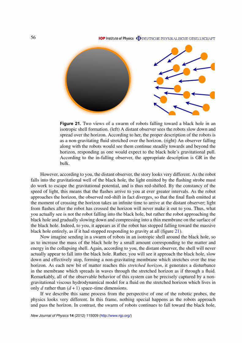
56

Figure 21. Two views of a swarm of robots falling toward a black hole in anisotropic shell formation. (left) A distant observer sees the robots slow down andspread over the horizon. According to her, the proper description of the robots isas a non-gravitating fluid stretched over the horizon. (right) An observer fallingalong with the robots would see them continue steadily towards and beyond thehorizon, responding as one would expect to the black hole’s gravitational pull.According to the in-falling observer, the appropriate description is GR in thebulk.

However, according to you, the distant observer, the story looks very different. As the robotfalls into the gravitational well of the black hole, the light emitted by the flashing strobe mustdo work to escape the gravitational potential, and is thus red-shifted. By the constancy of thespeed of light, this means that the flashes arrive to you at ever greater intervals. As the robotapproaches the horizon, the observed red-shift in fact diverges, so that the final flash emitted atthe moment of crossing the horizon takes an infinite time to arrive at the distant observer; lightfrom flashes after the robot has crossed the horizon will never make it out to you. Thus, whatyou actually see is not the robot falling into the black hole, but rather the robot approaching theblack hole and gradually slowing down and compressing into a thin membrane on the surface ofthe black hole. Indeed, to you, it appears as if the robot has stopped falling toward the massiveblack hole entirely, as if it had stopped responding to gravity at all (figure 21).

Now imagine sending in a swarm of robots in an isotropic shell around the black hole, soas to increase the mass of the black hole by a small amount corresponding to the matter andenergy in the collapsing shell. Again, according to you, the distant observer, the shell will neveractually appear to fall into the black hole. Rather, you will see it approach the black hole, slowdown and effectively stop, forming a non-gravitating membrane which stretches over the truehorizon. As each new bit of matter reaches this stretched horizon, it generates a disturbancein the membrane which spreads in waves through the stretched horizon as if through a fluid.Remarkably, all of the observable behavior of this system can be precisely captured by a non-gravitational viscous hydrodynamical model for a fluid on the stretched horizon which lives inonly d rather than (d + 1) space–time dimensions.

If we describe this same process from the perspective of one of the robotic probes, thephysics looks very different. In this frame, nothing special happens as the robots approachand pass the horizon. In contrast, the swarm of robots continues to fall toward the black hole,

New Journal of Physics 14 (2012) 115009 (http://www.njp.org/)

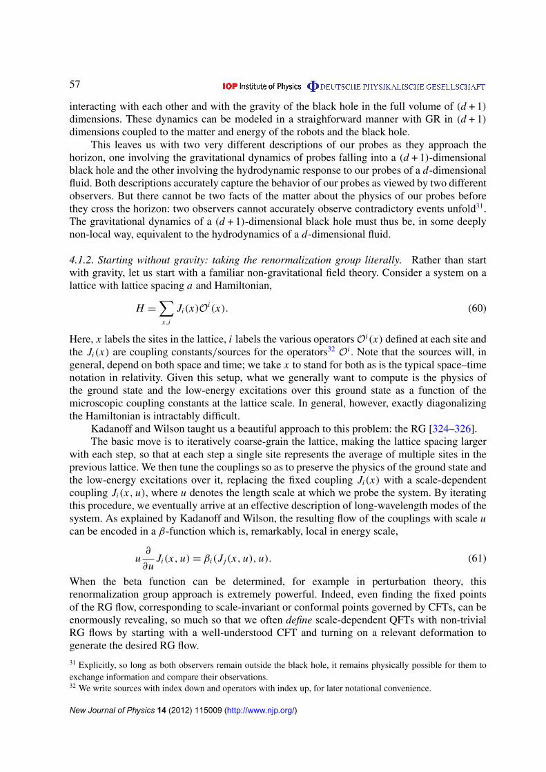
57

interacting with each other and with the gravity of the black hole in the full volume of (d + 1)dimensions. These dynamics can be modeled in a straighforward manner with GR in (d + 1)dimensions coupled to the matter and energy of the robots and the black hole.

This leaves us with two very different descriptions of our probes as they approach thehorizon, one involving the gravitational dynamics of probes falling into a (d + 1)-dimensionalblack hole and the other involving the hydrodynamic response to our probes of a d-dimensionalfluid. Both descriptions accurately capture the behavior of our probes as viewed by two differentobservers. But there cannot be two facts of the matter about the physics of our probes beforethey cross the horizon: two observers cannot accurately observe contradictory events unfold31.The gravitational dynamics of a (d + 1)-dimensional black hole must thus be, in some deeplynon-local way, equivalent to the hydrodynamics of a d-dimensional fluid.

4.1.2. Starting without gravity: taking the renormalization group literally. Rather than startwith gravity, let us start with a familiar non-gravitational field theory. Consider a system on alattice with lattice spacing a and Hamiltonian,

H =∑x,i

Ji(x)Oi(x). (60)

Here, x labels the sites in the lattice, i labels the various operatorsOi(x) defined at each site andthe Ji(x) are coupling constants/sources for the operators32 Oi . Note that the sources will, ingeneral, depend on both space and time; we take x to stand for both as is the typical space–timenotation in relativity. Given this setup, what we generally want to compute is the physics ofthe ground state and the low-energy excitations over this ground state as a function of themicroscopic coupling constants at the lattice scale. In general, however, exactly diagonalizingthe Hamiltonian is intractably difficult.

Kadanoff and Wilson taught us a beautiful approach to this problem: the RG [324–326].The basic move is to iteratively coarse-grain the lattice, making the lattice spacing larger

with each step, so that at each step a single site represents the average of multiple sites in theprevious lattice. We then tune the couplings so as to preserve the physics of the ground state andthe low-energy excitations over it, replacing the fixed coupling Ji(x) with a scale-dependentcoupling Ji(x, u), where u denotes the length scale at which we probe the system. By iteratingthis procedure, we eventually arrive at an effective description of long-wavelength modes of thesystem. As explained by Kadanoff and Wilson, the resulting flow of the couplings with scale ucan be encoded in a β-function which is, remarkably, local in energy scale,

u∂

∂uJi(x, u)= βi(J j(x, u), u). (61)

When the beta function can be determined, for example in perturbation theory, thisrenormalization group approach is extremely powerful. Indeed, even finding the fixed pointsof the RG flow, corresponding to scale-invariant or conformal points governed by CFTs, can beenormously revealing, so much so that we often define scale-dependent QFTs with non-trivialRG flows by starting with a well-understood CFT and turning on a relevant deformation togenerate the desired RG flow.

31 Explicitly, so long as both observers remain outside the black hole, it remains physically possible for them toexchange information and compare their observations.32 We write sources with index down and operators with index up, for later notational convenience.

New Journal of Physics 14 (2012) 115009 (http://www.njp.org/)

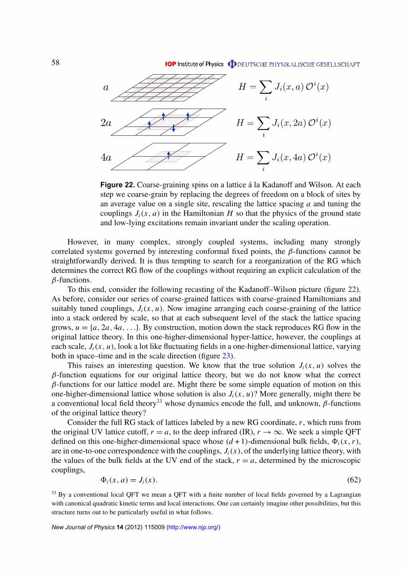
58

Figure 22. Coarse-graining spins on a lattice a la Kadanoff and Wilson. At eachstep we coarse-grain by replacing the degrees of freedom on a block of sites byan average value on a single site, rescaling the lattice spacing a and tuning thecouplings Ji(x, a) in the Hamiltonian H so that the physics of the ground stateand low-lying excitations remain invariant under the scaling operation.

However, in many complex, strongly coupled systems, including many stronglycorrelated systems governed by interesting conformal fixed points, the β-functions cannot bestraightforwardly derived. It is thus tempting to search for a reorganization of the RG whichdetermines the correct RG flow of the couplings without requiring an explicit calculation of theβ-functions.

To this end, consider the following recasting of the Kadanoff–Wilson picture (figure 22).As before, consider our series of coarse-grained lattices with coarse-grained Hamiltonians andsuitably tuned couplings, Ji(x, u). Now imagine arranging each coarse-graining of the latticeinto a stack ordered by scale, so that at each subsequent level of the stack the lattice spacinggrows, u = {a, 2a, 4a, . . .}. By construction, motion down the stack reproduces RG flow in theoriginal lattice theory. In this one-higher-dimensional hyper-lattice, however, the couplings ateach scale, Ji(x, u), look a lot like fluctuating fields in a one-higher-dimensional lattice, varyingboth in space–time and in the scale direction (figure 23).

This raises an interesting question. We know that the true solution Ji(x, u) solves theβ-function equations for our original lattice theory, but we do not know what the correctβ-functions for our lattice model are. Might there be some simple equation of motion on thisone-higher-dimensional lattice whose solution is also Ji(x, u)? More generally, might there bea conventional local field theory33 whose dynamics encode the full, and unknown, β-functionsof the original lattice theory?

Consider the full RG stack of lattices labeled by a new RG coordinate, r , which runs fromthe original UV lattice cutoff, r = a, to the deep infrared (IR), r→∞. We seek a simple QFTdefined on this one-higher-dimensional space whose (d + 1)-dimensional bulk fields, 8i(x, r),are in one-to-one correspondence with the couplings, Ji(x), of the underlying lattice theory, withthe values of the bulk fields at the UV end of the stack, r = a, determined by the microscopiccouplings,

8i(x, a)= Ji(x). (62)

33 By a conventional local QFT we mean a QFT with a finite number of local fields governed by a Lagrangianwith canonical quadratic kinetic terms and local interactions. One can certainly imagine other possibilities, but thisstructure turns out to be particularly useful in what follows.

New Journal of Physics 14 (2012) 115009 (http://www.njp.org/)

59

Figure 23. Holography promotes the tower of coarse-grained lattices to a one-higher-dimensional lattice, with the RG scale recast as a spatial dimension andthe running couplings Ji replaced by dynamical fields 8i which asymptoticallyapproach the ultraviolet (UV) couplings at the UV top of the stack and whichsatisfy a gravitational equation of motion in the bulk of the stack.

As a consequence, the bulk field8(x, r)must have the same charges, tensor structure and otherquantum numbers as the corresponding coupling34, Ji(x). Thus with each scalar operator O(x)is associated a bulk scalar field8(x, r) such that8(x, a)O(x) is a scalar operator we can add toour Hamiltonian, with each current operator J µ(x) is associated a bulk vector field, Aµ(x, r),such that Aµ(x, a)J µ(x) is a scalar and so forth. In particular, with the canonical stress-tensorT µν(x) is associated a canonical spin-2 field in the bulk, gµν(x, r).

What can the Lagrangian of this bulk QFT be? It is not the original latticeHamiltonian—the fields of the bulk QFT encode the dynamics of the couplings in RG space andnot of the operators on the original lattice. A priori, the natural thing to do is to write down themost general effective field theory allowed by the fields and symmetries of the system. However,a simple argument greatly constrains the possibilities. Any QFT defined by perturbation froma fixed point CFT as discussed above includes among its operators a canonical stress-energytensor, Tµν , arising as the Noether current corresponding to the space–time symmetry group. Thebulk QFT should thus include a corresponding canonical spin-2 field, gµν . But by the Weinbergand Weinberg–Witten theorems35 and assuming the existence of a Lorentz-invariant continuumlimit, any spin-2 field either must decouple at low energy, which would imply that sources of

34 Recall that our couplings are defined as the coefficients of the associated operators in the Hamiltonian, and sohave definite quantum numbers. Note too that, at fixed points of the β-functions where the system is scale invariant,the dimension of an operator is also a quantum number. This is also true in perturbations around such conformalfixed points.35 Weinberg [327] argued that any Lorentz-invariant theory of a spin-2 field must respect the equivalence principleor suffer IR pathologies; the Weinberg–Witten theorem [328] further states that any massless spin-2 field musteither be the graviton or suffer one of a host of pathologies, for example not having a conserved stress tensor. Foran illuminating discussion of these constraints, see [329] and references therein.

New Journal of Physics 14 (2012) 115009 (http://www.njp.org/)

60

momentum or energy in the original lattice theory do not affect the system, or must coupleuniversally according to the equivalence principle. In other words, the bulk field theory musteither be topological or be a theory of gravity that reduces, at long wavelength and low energy,to GR.

If all this can be done consistently, we would appear to have two distinct descriptions of oursystem: the original lattice theory with lattice spacing a and sources Ji(x) which satisfy first-order β-function equations; and a gravitational description living in a one-higher-dimensionalbulk whose fields, 8i(x, r), are in one-to-one correspondence with the sources Ji(x) but whichsatisfy conventional second-order local field equations. In other words, we have two ways tocompute correlation functions in our system: either we may work in the lattice theory and solvethe QFT problem; or we may work in the gravitational description and solve a GR problem.

In order for these two descriptions to have any chance of being equivalent36, the bulktheory must satisfy two among many rather unusual properties, both of which turn out tobe basic properties of black holes. Firstly, the entropy as computed in the two descriptionsmust be the same. In the original lattice QFT, the entropy will generically be extensive,with the entropy SQFT of the d-dimensional QFT in a region Rd scaling linearly with itsspatial volume, SQFT(Rd)∝ V (Rd). As a result, the entropy as measured in the one-greater-dimensional bulk gravity, SGR, must be sub-extensive, scaling as the area bounding a region,SGR(Rd+1)∝ A(Rd+1)∝ V (∂Rd+1). This is a basic feature of any theory of gravity37: the entropyin a volume is bounded by the entropy of a black hole that fits inside that volume [330]. Sincethe entropy of a black hole is proportional to the surface area of its horizon, SBH =

14 AH, this

tells us that the entropy of any region in a theory of gravity is bounded by its surface area,SGR(Rd)6

14 A(Rd). Indeed, the fact that the entropy of a black hole can be entirely associated

with its surface, and that as a result the entropy in gravity is necessarily sub-extensive, is theorigin of the term holography [331, 332]38.

Secondly, the β-function equations in the boundary lattice theory are first order in the scaler , while the gravitational equations of motion in the bulk are second order in r . Physically,this means that specifying the sources in the lattice QFT at one scale completely determinesthe coupling at all other scales, i.e. completely fixes the RG trajectory. By contrast, in thegravitational system we have two solutions to our second-order equation, so we must furtherspecify the derivative of the couplings with scale to uniquely fix the RG trajectory. How canthese be equivalent? Somehow it must be the case that the gravitational system automaticallyselects one of the two solutions of the bulk equations as physical.

It is again the physics of black holes which explains how this can happen. Imagine solvinga simple wave equation in the neighborhood of a black hole horizon. In principle, there aretwo solutions to the second-order wave equation. However, since things can fall into a black

36 By equivalent, we mean that their partition functions are exactly equal, so that both descriptions contain preciselythe same information, as we shall spell out in detail in section 4.2.3. Note that this implies their free energies andother thermodynamic data must similarly, and identically, match.37 Various other theories, including topological theories, share the property of sub-extensivity. However, byWeinberg–Witten, to have both an area law and an interacting spin-2 field, gravity appears to be the only option.38 The term holography is used by analogy with familiar holograms, and is meant to convey the surprising fact thatthe information about the (d + 1)-dimensional bulk space–time is being reliably encoded in the data of the QFTliving on the d-dimensional boundary. The analogy is in various ways quite apt. For example, information that islocal in the (d + 1)-dimensional bulk is encoded non-locally in the d-dimensional boundary. However, one shouldnot take the analogy too literally; for example, the encoding here involves quantum mechanics and gravity.

New Journal of Physics 14 (2012) 115009 (http://www.njp.org/)

61

hole horizon but nothing can escape, it is natural to organize the solutions near the horizon intoin-going and out-going waves. Moreover, when working in the Euclidean signature as is done,for example, in computing thermodynamic data, only the in-going solution is regular at thehorizon; the out-going solution is always irregular at the horizon. Thus, while the gravitationalfield equations are indeed second order, the presence of a black hole horizon effectively adds asecond boundary condition, so that we again need only specify a single boundary condition tocompletely determine the solution. Since the location of the horizon encodes the thermodynamicvariables (temperature, entropy) of the system, the physical meaning of this second boundarycondition is to specify the state of the QFT.

These heuristics suggest a connection between QFT in d space–time dimensions andquantum gravity in d + 1 space–time dimensions, with the fields in the gravitational systemexactly paired with sources in the dual QFT and with the extra spatial coordinate in thegravitational bulk playing the role of an RG scale. The next sections will describe a precise andcomputationally effective theory of this connection known as holographic duality and reviewsome of the lessons gleaned from its study to date.

4.1.3. Coda: the surprise of locality. It is worth pausing to contemplate just how remarkablethis proposal truly is. Consider a lattice theory in d-dimensions which has, in its Hamiltonian, areal parameter q. You might think of q as a global charge, or as a momentum, or something elseentirely, which can in principle be varied adiabatically. All correlation functions in the theoryare thus functions of d-dimensional space–time, (x, t), as well as of our parameter, q.

We might be tempted to take a stack of such lattices, each with a different value of q, callthe ‘space’ labeled by (x, t, q) a (d + 1)-dimensional space–time, and claim that the resultingtensor product of lattice QFTs is well described by a (d + 1)-dimensional QFT living on this(d + 1)-dimensional space–time.

This would be wrong. Being (d + 1)-dimensional means that all observables shouldtransform appropriately under translations, rotations, accelerations and general coordinatetransformations among x , t and q. They should also respect (d + 1)-dimensional causality andlocality. But that is absurd! What does it mean to rotate between the x direction and the qparameter? Meanwhile, there is absolutely no reason for correlators of two operators whichlive on lattices with very different values of q to vanish outside some q − t light cone, or foroperators from distant q-slices to have vanishing equal-time commutators in whatever state youchoose to call the ground state. Locality and causality are almost sure to be violated, and badly.This is not a (d + 1)-dimensional system.

To summarize, saying that the system is well described by a local, causal, unitary (d + 1)-dimensional QFT implies a long list of constraints on the (d + 1)-dimensional correlationfunctions. These translate into constraints on the original lattice theory and on the q-dependenceof its correlation functions. It is by no means obvious that any such stack of lattices can ever havea causal, local (d + 1)-dimensional description. From this point of view, holographic duality,in which the role of q is played by the energy scale and in which the (d + 1)-dimensionaldescription is in fact local, causal and even classical when the d-dimensional QFT is verystrongly interacting, is nothing short of astonishing. Precisely why, when and how this localityarises is perhaps the deepest question in holography39.

39 See, for example, [333] for a discussion of locality in holographic duality, and [334] for an interesting spin ofthe problem.

New Journal of Physics 14 (2012) 115009 (http://www.njp.org/)

62

4.2. Essential holography

Holographic duality [302–304] is a precise equivalence between certain d-dimensional quantumfield theories and (d + 1)-dimensional gravitational theories which provides a sharp realizationof the heuristics described in section 4.1. In particular, all the basic features noted above willreappear below: the fields in the bulk correspond to the couplings in the QFT; the RG flow ofthe QFT is encoded in the radial evolution of the gravitational theory along an extra dimension;and black hole horizons play a key role. Of particular importance is the precise geometry of theemergent space–time, as well as the precise relationship between observables in the QFT andthose of the gravitational dual. We will explore a few simple examples along the way.

For clarity of presentation, we will focus our discussion on the simplest possible QFTsfrom the point of view of the RG, i.e. Lorentz-invariant CFTs which are fixed points of theRG. Since the RG maps to radial evolution in the gravitational dual, QFTs corresponding to RGfixed points must be dual to geometries which are translationally invariant along the emergentradial direction up to overall rescalings; adding Lorentz invariance then entirely fixes the dualgeometry to be AdS, whose geometry we will now describe40.

4.2.1. Gravity and matter in anti-de Sitter space. AdSd+1 is a homogeneous, isotropicspace–time with d + 1 space–time dimensions and constant negative curvature whose metriccan be conveniently written as41

ds2=

L2

r 2

[−dt2 + dEx2 + dr 2

], (63)

where Ex are (d − 1) spatial coordinates, t is a time-like coordinate and r is a final ‘radial’ spatialcoordinate. The constant parameter L , known as the AdS-radius, sets the radius of curvature,with the Ricci curvature scalar given by the constant

R =−d(d + 1)

L2. (64)

The space is thus weakly curved when L is large and strongly curved when L is small. At fixedvalues of the radial coordinate r∗, the metric reduces to the d-dimensional Minkowski metric onflat space–time rescaled by L2/r 2

∗,

ds2r∗=

L2

r 2∗

[−dt2 + dEx2

]. (65)

It is thus useful to think of AdS as a stack of slices of flat space, with r controlling the physicalscale on that slice. The slice at r→ 0 is referred to as the boundary. Note that the volumeelement of the boundary slice at r→ 0 diverges, while the proper distance to the boundary alsodiverges. Thus the boundary at coordinate r→ 0 should be understood as the set of points atspatial infinity42.

40 The first examples of holographic duality involved such AdS/CFT dual pairs, and hence holographic duality isoften referred to as AdS/CFT. Just as we can always construct a general QFT by perturbing away from a CFT fixedpoint, we can extend such AdS/CFT dualities to more general QFTs and geometries by perturbing both sides incorresponding ways, so we do not lose too much by focusing on these examples.41 For the remainder of our discussion of holography we will work in natural units in which h = 1 and c = 1.42 In computations, it will often be useful to regulate this divergence by introducing a cutoff at r = a, with a� L ,removing the regulator, a→ 0, only at the end of all computations.

New Journal of Physics 14 (2012) 115009 (http://www.njp.org/)

63

Importantly, the full geometry is invariant under not just translations, rotations and Lorentzboosts along each slice, but also under general scaling transformations

(r, Ex, t)→ (αr, αEx, αt) (66)

as well as rotations and boosts that mix r with the other dimensions. The full isometry group ofAdSd+1 is, in fact, identical to the conformal group in d space–time dimensions43.

It is often useful to think of AdS as a harmonic trap for gravity. More precisely, the constantnegative curvature of AdS acts as a harmonic trap such that if you sit inside AdS at an arbitrarypoint and throw a ball, it will inevitably fall back to you in finite time. Indeed, if you fire out aphoton, that photon will run away to the boundary at r = 0 and return, again in finite observedtime44. And yet while nothing, not even gravity, gets out of the AdS box, the space–time remainscompletely homogeneous and isotropic. AdS thus acts as a peculiarly graceful IR regulator forgravity which breaks none of the symmetries of flat space.

All of this implies an intimate connection between the radial coordinate in the bulk ofAdS and spatial scales along the boundary: probing short distances (or high energies) along theboundary corresponds to probing the bulk only near the boundary at r = 0, while probing longdistances (or low energies) along the boundary corresponds to data deep in the interior of AdS.Roughly, then, we can think of the region near the boundary of AdS as associated with the UVphysics of the boundary, and of the deep interior of AdS as associated with the IR physics ofthe boundary.

To visualize this association, consider a fixed tension rope whose ends are glued to theboundary at r = 0. Due to the constant negative curvature of AdS, the bulk of the rope isdrawn into the bulk of the AdS space–time, forming an arc drooping away from the boundary.If the ends of the rope are held close together—probing short distances or high energy inthe four-dimensional (4D) boundary—the rope barely hangs into the bulk (figure 24). If weinstead pull the ends of the rope far apart—probing long distances or low energy in the 4Dboundary—the rope dips much further into the bulk. In this way, probing the IR of the boundarycorresponds to probing the deep interior of the AdS, r→∞, while probing the UV of theboundary corresponds to focusing on the near-boundary region of the geometry, r→ 0. Notethat the near-boundary cutoff at r = a� 1 thus acts as a UV regulator, while the horizon atr = rH provides a natural IR regulator.

Importantly, the AdS is a solution to the equations of motion of a generic Wilsonian actionfor the metric

IGravity =1

16πGN

∫dd+1x√−g

(−23 + R + c2 R2 + c3 R3 + · · ·

). (67)

Here, GN is the Newton constant, g is the determinant of the space–time metric, g = det(gµν),R is the Ricci curvature scalar built out of two derivatives of the metric, R ∼ ∂∂g, 3 is acosmological constant (also known as the tension of the vacuum), and the · · · represent allother scalars one can build out of the metric and its derivatives. The R term in the action playsthe role of a two-derivative kinetic term for the metric, gµν . GR is defined by retaining only the

43 Note that our regulator at r = a explicitly breaks conformal symmetry but does not break space–time rotationalor translational invariance in x and t , as a more conventional UV regulator such as a hard momentum cutoff would.Matching regulators between bulk and boundary turns out to be quite subtle, cf [335].44 Unlike the electromagnetic harmonic traps used in trapping cold atoms, AdS is homogeneous and isotropic:there is no center to which all objects return. Rather, the curvature ensures that any two initially parallel trajectoriesalways curve toward each other, no matter where they begin, and then oscillate.

New Journal of Physics 14 (2012) 115009 (http://www.njp.org/)

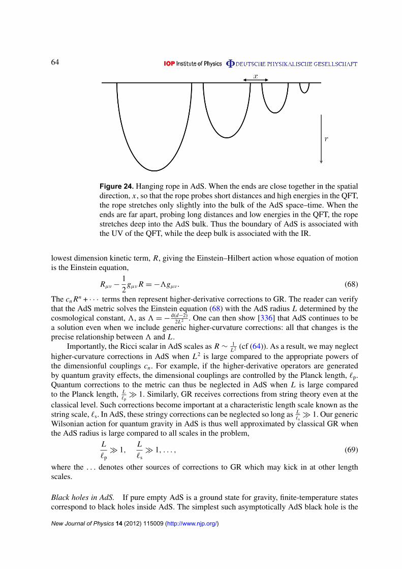
64

Figure 24. Hanging rope in AdS. When the ends are close together in the spatialdirection, x , so that the rope probes short distances and high energies in the QFT,the rope stretches only slightly into the bulk of the AdS space–time. When theends are far apart, probing long distances and low energies in the QFT, the ropestretches deep into the AdS bulk. Thus the boundary of AdS is associated withthe UV of the QFT, while the deep bulk is associated with the IR.

lowest dimension kinetic term, R, giving the Einstein–Hilbert action whose equation of motionis the Einstein equation,

Rµν −1

2gµνR =−3gµν. (68)

The cn Rn + · · · terms then represent higher-derivative corrections to GR. The reader can verifythat the AdS metric solves the Einstein equation (68) with the AdS radius L determined by thecosmological constant, 3, as 3=− d(d−2)

2L2 . One can then show [336] that AdS continues to bea solution even when we include generic higher-curvature corrections: all that changes is theprecise relationship between 3 and L .

Importantly, the Ricci scalar in AdS scales as R ∼ 1L2 (cf (64)). As a result, we may neglect

higher-curvature corrections in AdS when L2 is large compared to the appropriate powers ofthe dimensionful couplings cn. For example, if the higher-derivative operators are generatedby quantum gravity effects, the dimensional couplings are controlled by the Planck length, `p.Quantum corrections to the metric can thus be neglected in AdS when L is large comparedto the Planck length, L

`p� 1. Similarly, GR receives corrections from string theory even at the

classical level. Such corrections become important at a characteristic length scale known as thestring scale, `s. In AdS, these stringy corrections can be neglected so long as L

`s� 1. Our generic

Wilsonian action for quantum gravity in AdS is thus well approximated by classical GR whenthe AdS radius is large compared to all scales in the problem,

L

`p� 1,

L

`s� 1, . . . , (69)

where the . . . denotes other sources of corrections to GR which may kick in at other lengthscales.

Black holes in AdS. If pure empty AdS is a ground state for gravity, finite-temperature statescorrespond to black holes inside AdS. The simplest such asymptotically AdS black hole is the

New Journal of Physics 14 (2012) 115009 (http://www.njp.org/)

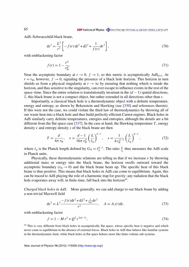
65

AdS–Schwarzchild black brane,

ds2=

L2

r 2

[− f (r) dt2 + dEx2 +

1

f (r)dr 2

], (70)

with emblackening factor

f (r)= 1−r d

r dH

. (71)

Near the asymptotic boundary at r→ 0, f → 1, so this metric is asymptotically AdSd+1. Atr = rH, however, f → 0, signaling the presence of a black hole horizon. This horizon in turnshields us from a physical singularity at r→∞ by ensuring that nothing which is inside thehorizon, and thus sensitive to the singularity, can ever escape to influence events in the rest of thespace–time. Since the entire solution is translationally invariant in the (d − 1) spatial directions,Ex , this black brane is not a compact object, but rather extended in all directions other than r .

Importantly, a classical black hole is a thermodynamic object with a definite temperature,energy and entropy, as shown by Bekenstein and Hawking (see [330] and references therein).If this were not the case, we could violate the third law of thermodynamics by throwing all ofour waste heat into a black hole and thus build perfectly efficient Carnot engines. Black holes inAdS similarly carry definite temperatures, energies and entropies, although the details are a bitdifferent from the flat space case [337]. In the case at hand, the Hawking temperature T , energydensity ε and entropy density s of the black brane are then

T =d

4π rH, ε =

d − 1

16π r dH

(L

`p

)d−1

, s =1

4 r d−1H

(L

`p

)d−1

, (72)

where `p is the Planck length defined by GN = `d−1p . The ratio L

`pthus measures the AdS scale

in Planck units.Physically, these thermodynamic relations are telling us that if we increase ε by throwing

additional mass or energy into the black brane, the horizon swells outward toward theasymptotic boundary (rH→ 0) and the black brane heats up. The specific heat of this blackbrane is thus positive. This means that black holes in AdS can come to equilibrium. Again, thiscan be traced to AdS playing the role of a harmonic trap for gravity: any radiation that the blackhole evaporates away will, in finite time, fall back into the horizon45.

Charged black holes in AdS. More generally, we can add charge to our black brane by addinga non-trivial Maxwell field

ds2= L2− f (r)dt2 + dEx2 + 1

f(r)dr 2

r 2, A = At(r)dt, (73)

with emblackening factor

f = 1−M r d + Q2 r 2(d−1), (74)

45 This is very different from black holes in asymptotically flat space, whose specific heat is negative and whichnever come to equilibrium in the absence of external forces. Black holes in AdS thus behave like familiar systemsin the thermodynamic limit, while black holes in flat space behave more like finite-volume sub-systems.

New Journal of Physics 14 (2012) 115009 (http://www.njp.org/)

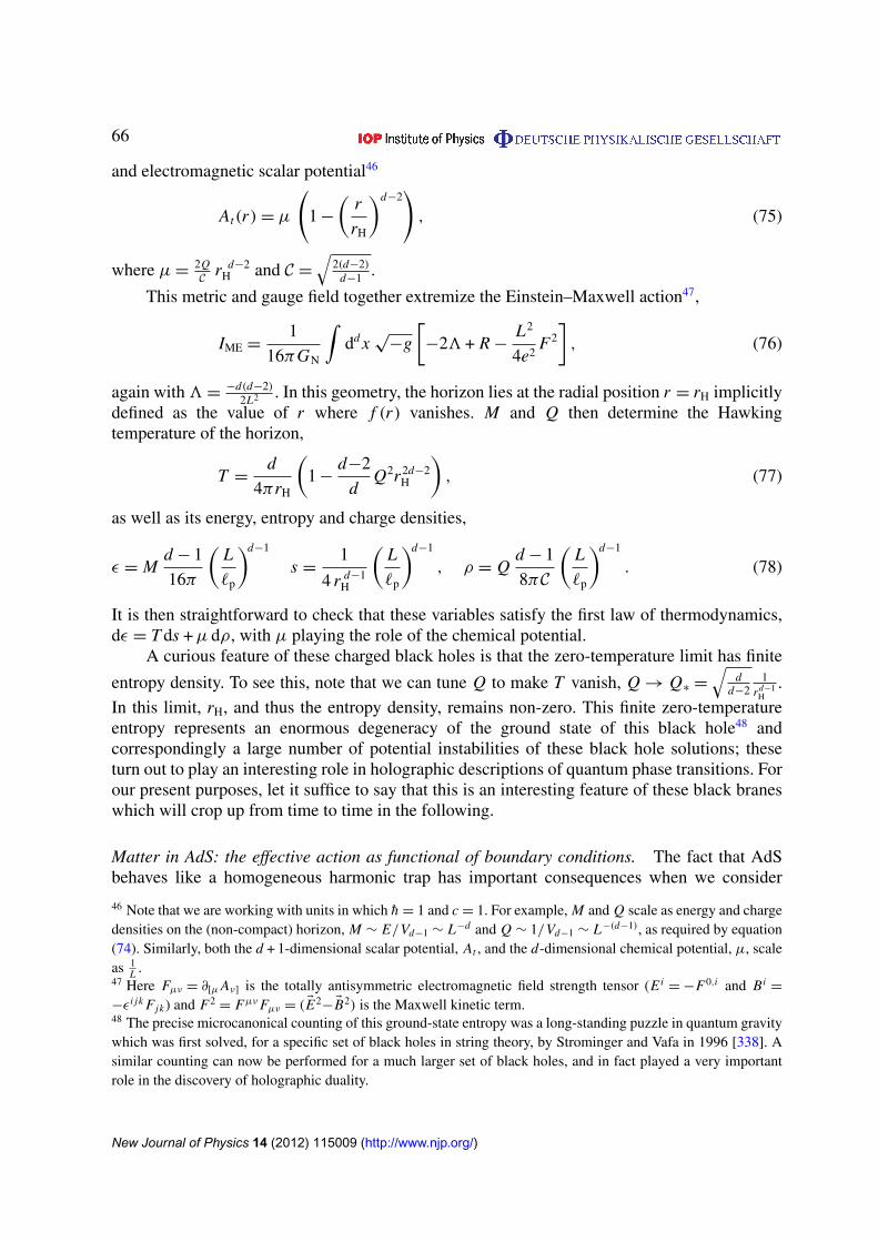
66

and electromagnetic scalar potential46

At(r)= µ

(1−

(r

rH

)d−2), (75)

where µ= 2QC r d−2

H and C =√

2(d−2)d−1 .

This metric and gauge field together extremize the Einstein–Maxwell action47,

IME =1

16πGN

∫dd x√−g

[−23+ R−

L2

4e2F2

], (76)

again with3= −d(d−2)2L2 . In this geometry, the horizon lies at the radial position r = rH implicitly

defined as the value of r where f (r) vanishes. M and Q then determine the Hawkingtemperature of the horizon,

T =d

4πrH

(1−

d−2

dQ2r 2d−2

H

), (77)

as well as its energy, entropy and charge densities,

ε = Md − 1

16π

(L

`p

)d−1

s =1

4 r d−1H

(L

`p

)d−1

, ρ = Qd − 1

8πC

(L

`p

)d−1

. (78)

It is then straightforward to check that these variables satisfy the first law of thermodynamics,dε = T ds +µ dρ, with µ playing the role of the chemical potential.

A curious feature of these charged black holes is that the zero-temperature limit has finite

entropy density. To see this, note that we can tune Q to make T vanish, Q→ Q∗ =√

dd−2

1rd−1

H.

In this limit, rH, and thus the entropy density, remains non-zero. This finite zero-temperatureentropy represents an enormous degeneracy of the ground state of this black hole48 andcorrespondingly a large number of potential instabilities of these black hole solutions; theseturn out to play an interesting role in holographic descriptions of quantum phase transitions. Forour present purposes, let it suffice to say that this is an interesting feature of these black braneswhich will crop up from time to time in the following.

Matter in AdS: the effective action as functional of boundary conditions. The fact that AdSbehaves like a homogeneous harmonic trap has important consequences when we consider

46 Note that we are working with units in which h = 1 and c = 1. For example, M and Q scale as energy and chargedensities on the (non-compact) horizon, M ∼ E/Vd−1 ∼ L−d and Q ∼ 1/Vd−1 ∼ L−(d−1), as required by equation(74). Similarly, both the d + 1-dimensional scalar potential, At , and the d-dimensional chemical potential, µ, scaleas 1

L .47 Here Fµν = ∂[µAν] is the totally antisymmetric electromagnetic field strength tensor (E i

=−F0,i and Bi=

−εi jk F jk) and F2= FµνFµν = ( EE2

−EB2) is the Maxwell kinetic term.48 The precise microcanonical counting of this ground-state entropy was a long-standing puzzle in quantum gravitywhich was first solved, for a specific set of black holes in string theory, by Strominger and Vafa in 1996 [338]. Asimilar counting can now be performed for a much larger set of black holes, and in fact played a very importantrole in the discovery of holographic duality.

New Journal of Physics 14 (2012) 115009 (http://www.njp.org/)

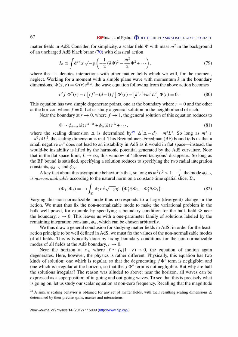
67

matter fields in AdS. Consider, for simplicity, a scalar field 8 with mass m2 in the backgroundof an uncharged AdS black brane (70) with classical action

I8 ∝∫

dd+1x√−g

(−

1

2(∂8)2−

m2

282 + · · ·

), (79)

where the · · · denotes interactions with other matter fields which we will, for the moment,neglect. Working for a moment with a simple plane wave with momentum k in the boundarydimensions,8(x, r)=8(r)eik·x , the wave equation following from the above action becomes

r 2 f 8′′(r)− r[r f ′−(d−1) f

]8′(r)−

[k2r 2+m2L2

]8(r)= 0. (80)

This equation has two simple degenerate points, one at the boundary where r = 0 and the otherat the horizon where f = 0. Let us study a general solution in the neighborhood of each.

Near the boundary at r→ 0, where f → 1, the general solution of this equation reduces to

8∼ φd−1(k) r d−1 +φ1(k) r1 + · · · , (81)

where the scaling dimension 1 is determined by49 1(1− d)= m2L2. So long as m2 >−d2/4L2, the scaling dimension is real. This Breitenloner–Freedman (BF) bound tells us that asmall negative m2 does not lead to an instability in AdS as it would in flat space—instead, thewould-be instability is lifted by the harmonic potential generated by the AdS curvature. Notethat in the flat space limit, L→∞, this window of ‘allowed tachyons’ disappears. So long asthe BF bound is satisfied, specifying a solution reduces to specifying the two radial integrationconstants, φd−1 and φ1.

A key fact about this asymptotic behavior is that, so long as m2L2 > 1− d2

4 , the mode φd−1

is non-normalizable according to the natural norm on a constant-time spatial slice, 6t ,

(81,82)=−i∫6t

dz dEx√−ggt t

(8∗1∂t82−8

∗

2∂t81

). (82)

Varying this non-normalizable mode thus corresponds to a large (divergent) change in theaction. We must thus fix the non-normalizable mode to make the variational problem in thebulk well posed, for example by specifying a boundary condition for the bulk field 8 nearthe boundary, r→ 0. This leaves us with a one-parameter family of solutions labeled by theremaining integration constant, φ1, which can be chosen arbitrarily.

We thus draw a general conclusion for studying matter fields in AdS: in order for the least-action principle to be well defined in AdS, we must fix the values of the non-normalizable modesof all fields. This is typically done by fixing boundary conditions for the non-normalizablemodes of all fields at the AdS boundary, r→ 0.

Near the horizon at rH, where f ∼ fH (1− r)→ 0, the equation of motion againdegenerates. Here, however, the physics is rather different. Physically, this equation has twokinds of solution: one which is regular, so that the degenerating f8′′ term is negligible; andone which is irregular at the horizon, so that the f8′′ term is not negligible. But why are halfthe solutions irregular? The reason was alluded to above: near the horizon, all waves can beexpressed as a superposition of in-going and out-going waves. To see that this is precisely whatis going on, let us study our scalar equation at non-zero frequency. Recalling that the magnitude

49 A similar scaling behavior is obtained for any set of matter fields, with their resulting scaling dimensions 1determined by their precise spins, masses and interactions.

New Journal of Physics 14 (2012) 115009 (http://www.njp.org/)

68

of the d-momentum k in the metric (70) is k2=−

r2

f ω2 + r 2Ek2, the dominant terms in the scalar

equation near the horizon are

f ∂r( f ∂r8)+ω28∼ 0. (83)

It is useful to switch to the near-horizon coordinate ρ defined by f ∂r = ∂ρ , i.e. e−ρ ∼ (1− r)1/ fH ,in terms of which the horizon lies at ρ→∞. In terms of this coordinate, the general solutioncan be expressed as a superposition of in-going and out-going waves as

8=8in(ρ) e−iω(t−ρ) +8out(ρ) e−iω(t+ρ). (84)

For future reference, note that the in(out)-going solutions satisfy the first-order constraint at rH,

f ∂r8in = iω8in, f ∂r8out =−iω8out. (85)

Note that, in terms of the original radial coordinate, r , the phases of both of these time-dependentsolutions accumulate near the horizon. One can check that, in the limit of zero frequency, thein-going wave is regular at the horizon while the out-going wave is irregular, matching ourzero-frequency analysis above. Note, too, that this suggests a natural prescription for analyticcontinuation to Euclidean time: we should choose the continuation so that the in-going wave isregular at the Euclidean horizon, eiωρ

→ e−ωEρ , i.e. we should define ω = iωE, where ωE > 0.Again, this turns out to be a general result: in the presence of a black hole horizon, the

Laplacian in any tensor representation takes the form�∼ r 2 f ∂2r + r2ω2

f + . . ., so we must imposea boundary condition on our solutions such that they correspond to regular, in-falling modes atthe horizon.

Thus, while our equation of motion is second order, there is only one linearly independentsolution which is regular everywhere in the bulk and in-going at the horizon. Our gravityproblem in AdS, in the presence of a black hole horizon, becomes effectively a first-orderproblem50. Explicitly, fixing the non-normalizable mode φd−1 at the boundary and imposingin-falling boundary conditions at the horizon completely determines our solution for 8throughout the bulk of AdS and as a result determines φ1. However, in order to actually computeφ1 given φd−1, we must solve our problem not just at the boundary but all the way through thebulk to the horizon, where we impose the appropriate boundary conditions. The relation betweenφd−1 and φ1 is thus also determined by IR physics and not just UV physics.

It is illuminating to see this work in detail in an analytically solvable example. Consideragain our scalar field 8 but now in pure AdS, i.e. with no black hole. This correspondsto studying our dual QFT at zero temperature and zero density. Expanding in plane waves,e−i(ωt−kx), the general solution to the bulk equation of motion can be found in closed form

8(t, x, r)=[φreg r

d2 Kν (κr)+φirreg r

d2 Iν (κr)

]e−i(ωt−kx), (86)

where ν =1− d2 , κ =

√ω2 + Ek2, Kν and Iν are modified Bessel functions and φreg and φirreg are

the two integration constants. Since Iν(κr)∼ eκr near the ‘AdS horizon’ at r→∞, regularityrequires that φirreg = 0. We thus have just a single integration constant, φreg, which fixes theoverall normalization of the in-falling mode in 8. Near the boundary, the two asymptoticintegration constants φd−1 and φ1 in (81) are not independent. We can see how they are related

50 A similar story holds for fermions, although the details differ because the Dirac equation is naturally firstorder [339].

New Journal of Physics 14 (2012) 115009 (http://www.njp.org/)

69

by setting φirreg = 0 in (86) and expanding the solution near the boundary. After a little algebra,this gives

φ1 =0(d

2 −1)

21−d20(1− d

2 )

(ω2 + k2

)1− d2 φd−1. (87)

Thus, once we impose regularity on our bulk solutions, we need only one boundary conditionin the UV at r→ 0 to fully specify a solution of the second-order bulk equations of motion.Meanwhile, we know that we need to fix the non-normalizable mode φd−1 at the boundary sothat our variational problem is well posed. Once we impose regularity in the bulk, i.e. in-fallingat the horizon, the value of φ1 is completely determined.

This teaches us an important lesson. Suppose that we want to study the partition functionfor our gravitational theory in AdS, integrating over all bulk fields, 8(x, r). To make thevariational problem well posed, we must specify a boundary condition for each of the bulkfields at the boundary of AdS, as discussed above,

φd−1(x)= limr→0

r1−d8(x, r), (88)

where the factor of r1−d should be thought of as the appropriate wavefunction renormalizationof the bulk field 8(x, r). This means that the partition function in AdS, and thus the effectiveaction 0AdS =−ln[ZAdS], is a functional of the boundary conditions for all bulk fields,

ZAdS[φd−1(x)]≡ ZAdS[8[φd−1(x)]]. (89)

What one means by ‘a theory of gravity in AdS’. In discussing holography, we will regularlyrefer to classical gravity, quantum gravity and perturbative gravity in AdS, so it is worth takinga moment to define our terms here.

By quantum gravity in AdS we mean a complete quantum description of the gravitationalsystem, i.e. string theory in AdS. In general, string theory is a rich and complicated quantumtheory which has no simple perturbative classical description. However, in some cases closedstrings have a tractable semiclassical low-energy expansion involving a metric, gµν , minimallycoupled to a host of dynamical matter fields, {8i}, governed by an effective action of the form

IGR =1

16πGN

∫dd+1x√−g (−23+ R + · · ·+Lmatter(8i)) . (90)

Here Lmatter(8i) is the Lagrangian density for the matter fields and R is the Ricci curvaturescalar, which is roughly two derivatives of the metric.

√gR plays the role of a kinetic term for

the metric in GR. The · · · then represents an infinite tower of higher-derivative terms involvingthe metric, for example R2, R4, etc, which represent closed string corrections to GR. Since thesehigher-derivative terms are also higher-dimension irrelevant operators, they must appear withdimensionful couplings. In general, these couplings are controlled by two independent lengthscales: `p, the Planck length, which controls quantum corrections to the dynamics of classicalstrings; and `s, which controls classical ‘stringy’ corrections to the dynamics of point particles.

When expanding the theory around AdS with AdS-length L (and thus with Ricci curvatureR ∼ L−2), we thus have two dimensionless parameters controlling the various possiblecorrections to GR: `p

L , which tells us whether quantum corrections are important; and `sL , which

tells us whether stringy corrections are important. Note that ensuring that the curvature is weakin Planck units, `p

L � 1, does ensure that the system can be treated classically, but does not tell

New Journal of Physics 14 (2012) 115009 (http://www.njp.org/)

70

us that the gravity must be exactly GR: the curvature of our AdS may still be large compared tothe string scale, so higher-curvature corrections to the Lagrangian of GR may not be negligible.For pure classical GR to be a good approximation, two independent conditions must thus hold,

`p

L� 1 and

`s

L� 1, (91)

i.e. the curvature must be small compared both to the Planck scale and to the string scale.

4.2.2. Field theories in flat space. Our next job is to define the d-dimensional QFT we wantto study. A canonical way to do so begins by specifying a list of local operators Oi labeled bytheir Lorentz structure, their charges qi and their scaling dimensions1i , all defined at some UVfixed point. To generate an RG flow of interest, we perturb away from this fixed point by turningon appropriate sources Ji . The basic observables of the theory are then correlation functions ofproducts of local operators

〈O1(x1) . . .On(xn)〉. (92)

These can be conveniently encoded in terms of the quantum generating functional,

ZQFT[Ji(x)]= 〈e∫

dxd Ji (x)Oi (x)〉, (93)

where the Ji(x) represent a set of sources and couplings for the operators Oi . Note that thescaling dimensions and tensor structure of the sources Ji are completely determined by those ofOi . This allows us to express correlation functions as derivatives of the partition function

〈O1(x1) . . .On(xn)〉 =δn ln ZQFT[J (x)]

δ J1(x1) . . . δ Jn(xn)

∣∣∣Ji=0, (94)

where the restriction |Ji=0 means that evaluate the final result with all remaining sources turnedoff. Solving the theory then requires one to compute the partition function, ZQFT[Ji(x)].

Canonical example: SU (N ) Yang–Mills at large N. The classic example of a field theorywith a well-understood and controlled holographic dual, to which we will appeal below, is aspecial version of the SU (N ) Yang–Mills gauge theory in flat 4D space–time called the N = 4theory. HereN refers to the amount of supersymmetry enjoyed by the theory;N = 4 is the mostone can have in 4D without including gravity. For our purposes, the role of supersymmetryis nothing more than a way of turning off quantum mechanics without totally trivializing thetheory: withN = 4 supersymmetry, some quantities do not receive quantum corrections beyondone loop, and so can be computed at weak coupling and reliably extrapolated to strong coupling.In particular, the b-function of the theory can be computed exactly and is identically zero for allvalues of the coupling51.

The basic ingredients of the N = 4 theory are a gauge group, G = SU (N ), a gauge field,Aµ(x), transforming in the adjoint of G, six scalars φ I (x) also transforming in the adjoint of

51 Our ability to compute various quantities at both strong and weak coupling in the N = 4 theory was key to theoriginal discovery of holographic duality, and is the reason why this example is both illuminating and canonical.However, that is the extent of the role of supersymmetry, to provide unusually simple and tractable examples. Itis no more a necessary feature of holography than spherical symmetry is a necessary property of hydrogen. Themaximally supersymmetricN = 4 theory is an illuminating example to study, so we turn to it now, but we stress thatthe general structure of holographic duality thus revealed is more general, and does not depend on supersymmetry.

New Journal of Physics 14 (2012) 115009 (http://www.njp.org/)

71

G and further enjoying a global SO(6) symmetry, and a large set of fermions. We can safelyneglect the fermions for now, as their only role is to ensure supersymmetry. The Lagrangian is

LYM =−1

4g2

(Tr F2 + Tr |DφI |

2 + · · ·), (95)

where g2YM is the gauge coupling, Dµ is the gauge-covariant derivative, · · · denotes fermionic

terms we neglect and all fields are canonically normalized with an overall factor of− 14g2 in front

of their kinetic terms.What are the good operators of this theory? We may suppose that any good gauge-invariant

combination of the fundamental fields is a perfectly good observable. However, since we have aglobal symmetry, it is useful to write this list in terms of SO(6) irreducible representations. Forexample, the following three Lorentz scalars,

O =∑

I

Trφ2I , OI J = Trφ(IφJ ), Oµ = TrJ µ, (96)

transform as a scalar, a symmetric two-tensor and a vector, respectively, under the globalSO(6), with the latter corresponding to a charge current operator. In the weak-coupling limit,their scaling dimensions 1i are just their engineering dimensions which can be read off theLagrangian52.

Now, as pointed out by ’t Hooft [341] (see also [342]), anytime you have a gauge theory ofN × N matrices, there is a natural way to organize the Feynman diagrams in terms of underlyinggenus-g surfaces53. Explicitly, since every field comes with two gauge indices, and since allindices in a gauge invariant observable must be contracted, every Feynman diagram can bewritten as a ribbon diagram in which each propagator is a ribbon with a gauge running alongeach side of the ribbon. One can then show that any given Feynman diagram, with any numberof underlying loops, can be drawn without the index lines crossing only on a genus-g Riemannsurface, where the specific genus g depends on precisely how the index lines are contracted tomake the given Feynman diagram. Explicitly, a diagram with genus g = 0 can be drawn on apiece of paper with no lines crossing, a diagram of genus g = 1 must be drawn on a torus tohave no lines cross, etc.

A remarkable result is that if we reorganize the loop expansion in g2YM as a double

expansion in N and λ= g2YM N , then every observable can be expressed as a power series

expansion in N where the powers of N for a given diagram is determined only by the genus gon which that diagram can be drawn with no crossings. For example, the free energy F = ln Ztakes the form

F = N 2 f0(λ)+ f1(λ)+1

N 2f2(λ)+ · · · = N 2

∑g

fg(λ)

N 2g, (97)

where fg(λ) is the sum of all diagrams arising at genus g and is a function of only λ, independentof N . A similar result is obtained for every possible observable, with the only difference being

52 Here, engineering dimension refers to the naive dimension of an operator as determined by dimensional analysison the kinetic terms in the classical Lagrangian, while the true scaling dimension is determined by the scaledependence of correlation functions containing the operator in the full interacting quantum theory. For a review ofengineering and general scaling dimensions, see, e.g., the text by Sachdev [340].53 Here the genus refers to the number of handles on a two-dimensional surface: a sphere or plane has genus zero,a donut has genus 1, a donut with two holes has genus 2, etc.

New Journal of Physics 14 (2012) 115009 (http://www.njp.org/)

72

the overall factor of N ,

A= N m

(A0(λ)+

1

N 2A1(λ)+

1

N 4A2(λ)+ · · ·

)= N m

∑g

Ag(λ)

N 2g. (98)

This double expansion implies a remarkable simplification at large N : if N � 1, the only termthat matters in the genus expansion is the leading planar term; any diagram that cannot be drawnon a piece of paper without crossings, while possibly large in numerical value, is dwarfed bythe much larger terms coming from the planar diagrams.

Another way of expressing this simplification at large N is on terms of large Nfactorization. Consider a set of single-trace operators54 of the form Oi = Tr (. . .). At large N ,correlation functions of single trace operators factorize

〈O1(x1)O2(x2)〉 = 〈O1(x1)〉〈O2(x2)〉+ O

(1

N 2

). (99)

This follows because the disconnected parts of the diagrams necessarily involve more closedindex loops than connected parts and thus additional powers of N . This does not imply that thelarge N theory is free, for while these correlators do factorize, the individual one-point functionsremain non-trivial. For example, the anomalous dimensions of all operators are controlled bythe ’t Hooft coupling, λ.

We thus see that large N gauge theories have two natural coupling constants: 1N ,

which controls the genus expansion and factorization; and λ, which controls the perturbativecorrections to each term in the genus expansion and the anomalous dimensions of large Nfactorized operators. Suggestively, this is precisely the structure of closed string perturbationtheory, where every amplitude is expressed as a sum of contributions from various genera, withthe loop-counting parameter given by the string coupling gs and the amplitude of a given genusdetermined by an auxiliary QFT whose interactions are determined by the string tension α′ viathe relation

A= gns

(A0(α

′)+ g2sA1(α

′)+ g4sA2(α

′)+ · · ·)= gn

s

∑g

g2gs Ag(α

′). (100)

This analogy led various people to speculate that large N gauge theories should be captured bysome theory of closed strings. This turned out to be wrong, but only just barely: at large N , thesetheories are dual to closed string theories, but the closed strings live in one higher dimension!

As an aside, while not every theory is a gauge theory of N × N matrices, it is useful to keepin mind this example when thinking about more general examples. What N 2 is really measuringis the number of degrees of freedom per unit volume, or per lattice site if we put the theory on alattice. Similarly, λ is measuring the strength of the dominant interactions when the number ofdegrees of freedom grows large. Many theories that are not simple gauge theories, nonetheless,have a useful notion of N and λ. Exactly when one obtains such a controlled double expansionremains, in general, a key open question in holography.

4.2.3. The holographic dictionary. The basic claim of holography is that every d-dimensionalQFT defined as above can be exactly reorganized into a (d + 1)-dimensional quantum theory ofgravity and matter propagating in AdSd+1. The precise relationship between these two theoriesis known as the holographic dictionary, a sketch of which is outlined in table 1. The rest of this

54 The meaning of single-trace operators is slightly subtle, but can roughly be understood as the set of operatorswhich have local, extensive classical limits.

New Journal of Physics 14 (2012) 115009 (http://www.njp.org/)

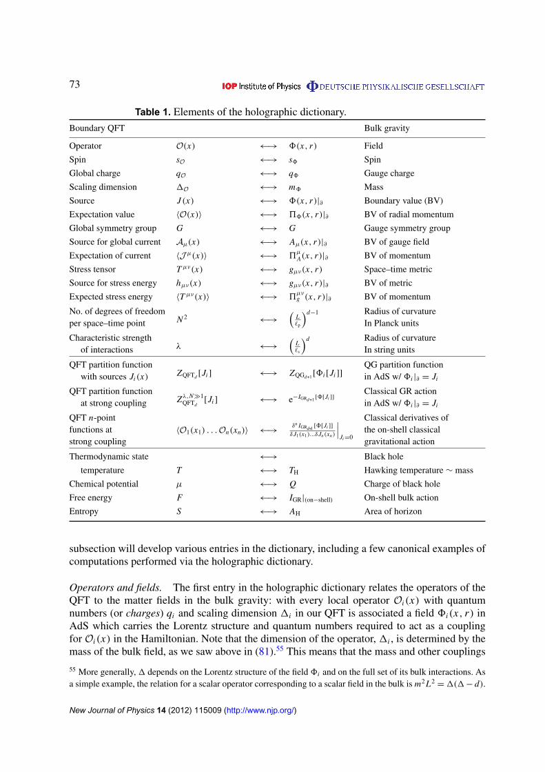
73

Table 1. Elements of the holographic dictionary.

Boundary QFT Bulk gravity

Operator O(x) ←→ 8(x, r) Field

Spin sO ←→ s8 Spin

Global charge qO ←→ q8 Gauge charge

Scaling dimension 1O ←→ m8 Mass

Source J (x) ←→ 8(x, r)|∂ Boundary value (BV)

Expectation value 〈O(x)〉 ←→ 58(x, r)|∂ BV of radial momentum

Global symmetry group G ←→ G Gauge symmetry group

Source for global current Aµ(x) ←→ Aµ(x, r)|∂ BV of gauge field

Expectation of current 〈J µ(x)〉 ←→ 5µ

A(x, r)|∂ BV of momentum

Stress tensor T µν(x) ←→ gµν(x, r) Space–time metric

Source for stress energy hµν(x) ←→ gµν(x, r)|∂ BV of metric

Expected stress energy 〈T µν(x)〉 ←→ 5µνg (x, r)|∂ BV of momentum

No. of degrees of freedomN 2

←→

(L`p

)d−1 Radius of curvatureper space–time point In Planck units

Characteristic strengthλ ←→

(L`s

)d Radius of curvatureof interactions In string units

QFT partition functionZQFTd

[Ji ] ←→ ZQGd+1[8i [Ji ]]

QG partition functionwith sources Ji (x) in AdS w/ 8i |∂ = Ji

QFT partition functionZλ,N�1

QFTd[Ji ] ←→ e−IGRd+1 [8[Ji ]]

Classical GR actionat strong coupling in AdS w/ 8i |∂ = Ji

QFT n-point〈O1(x1) . . .On(xn)〉 ←→

δn IGRd+1 [8[Ji ]]δ J1(x1)...δ Jn(xn)

∣∣∣Ji=0

Classical derivatives offunctions at the on-shell classicalstrong coupling gravitational action

Thermodynamic state ←→ Black hole

temperature T ←→ TH Hawking temperature ∼ mass

Chemical potential µ ←→ Q Charge of black hole

Free energy F ←→ IGR|(on−shell) On-shell bulk action

Entropy S ←→ AH Area of horizon

subsection will develop various entries in the dictionary, including a few canonical examples ofcomputations performed via the holographic dictionary.

Operators and fields. The first entry in the holographic dictionary relates the operators of theQFT to the matter fields in the bulk gravity: with every local operator Oi(x) with quantumnumbers (or charges) qi and scaling dimension 1i in our QFT is associated a field 8i(x, r) inAdS which carries the Lorentz structure and quantum numbers required to act as a couplingfor Oi(x) in the Hamiltonian. Note that the dimension of the operator, 1i , is determined by themass of the bulk field, as we saw above in (81).55 This means that the mass and other couplings

55 More generally,1 depends on the Lorentz structure of the field8i and on the full set of its bulk interactions. Asa simple example, the relation for a scalar operator corresponding to a scalar field in the bulk is m2L2

=1(1− d).

New Journal of Physics 14 (2012) 115009 (http://www.njp.org/)

74

of the bulk gravity theory generally do not correspond to interactions of the boundary theory inany simple way, but rather determine which boundary QFT we are studying.

An equivalence of partition functions. Given this map, the central claim of holographicduality [302–304] can be succinctly expressed as

ZQFT[Ji ]= ZQG[8[Ji ]], (101)

where ZQFT[Ji ] is the partition function of the QFT as a function of the sources Ji foreach operator Oi , while ZQG[8[Ji ]] is the quantum partition function of the gravitationaltheory described in section 4.2.1 computed in an AdS space–time background56. As discussed,the quantum gravity partition function must be evaluated on field configurations 8i whichasymptote at the boundary to the sources Ji of the QFT, hence the notation 8[J ]. As in theheuristic derivation above, the bulk fields are precisely the coupling constants of the QFTpromoted to dynamical fields on the full RG-extended space–time in which the RG scalebecomes a physical coordinate.

An important ingredient in this recipe is a proper definition of the boundary value of thebulk field. As we saw above for a bulk scalar 8 of mass m, dual to a scalar operator O ofdimension 1 given by 1(d −1)= m2L2, the boundary value of the bulk field is in generaldivergent. To specify the boundary condition, we must rescale the bulk field by an appropriatewavefunction renormalization which picks off the leading divergence of the bulk field near theboundary

J (x)≡ φd−1(x)= limr→0

r1−d8(x, r). (102)

We will return to this renormalization when we discuss the computation of one- and two-pointfunctions.

Strong coupling and perturbative gravity. In general, both sides of equation (101) arecomplicated and computationally intractable objects. However, when one side or the othercan be evaluated semi-classically, we can use equation (101) to generate a controlled strong-coupling expansion via the dual description. Precisely whether, and when, such a limit isobtained is a delicate question that must be studied in detail on a case-by-case basis. To geta sense of the general structure, let us consider the canonical example, the large N limit of the4DN = 4 gauge theory with gauge group G = SU (N ) and ’t Hooft coupling λ. The dual theoryturns out to be a closed string theory on AdS5 with AdS-radius L . The holographic dictionarythen tells us that

N 2=

(L

`p

)d−1

, λ=

(L

`s

)d

, (103)

where `p is the Planck length determining the scale at which quantum effects occur in the bulk,and `s is the string length controlling the scale of stringy higher-curvature corrections to thebulk gravitational action, as discussed in section 4.2.1. The first relation in equation (103) thustells us that the bulk description becomes classical (L � `p) only in the large-N limit57 and that

56 In general, ZQG means the partition function of closed string theory expanded around the AdS geometry. Inpractice, we can only compute this explicitly in special cases and then only in regimes in which the string couplingand curvature are sufficiently weak. Thus, we may use this duality either to deduce the lhs of equation (101) whenthe gravity is classical and weakly curved or to define the rhs of equation (101) when the QFT is computable.57 This provides an out from the Weinberg–Witten argument, which assumes that there are a finite number of localdegrees of freedom.

New Journal of Physics 14 (2012) 115009 (http://www.njp.org/)

75

the gravitational description is deeply quantum mechanical when N is small. In other words,the loop counting parameter in the bulk is 1

N .With an eye toward the general class of holographic theories, it is worthwhile unpacking

equation (103) in more detail. In the case at hand, i.e. SU (N ) SYM, N 2 measures the number ofdegrees of freedom per point in the QFT. In particular, all extensive thermodynamic quantities(entropy, energy, etc) must scale as N 2. In this light, what equation (103) shows is that thequantum corrections in the bulk are negligible when the number of degrees of freedom per pointin the dual QFT is large, and vice versa. Indeed, in a host of controlled models in string theory,the appropriate version of the first equation in equation (103) takes the form, N b

=(L/`p

)d−1,

where N is a conserved charge and b is some real parameter [343]. Similarly, it is not alwayspossible to interpret λ as a ’t Hooft parameter in the dual QFT. More generally, the role of λis played by the typical scale of anomalous dimensions in the QFT [333]. We can understandthis as follows: if the QFT is weakly interacting, the effects of renormalization will generally beweak and most observables will be well approximated by their classical cousins, i.e. quantumanomalous dimensions will be small; if interactions are strong, quantum effects will generallydrive anomalous dimensions to be large.

While N � 1 ensures that the Planck scale is negligible, so that the gravitationalinteractions can be treated with classical effective field theory, it does not tell us that thesystem is well approximated by pure GR. Indeed, in principle, there will be a host of higher-curvature corrections to the classical GR action suppressed by powers of `s

L . To ensure thatthese corrections are in fact negligible, i.e. that L � `s, we must furthermore take the ’t Hooftcoupling to be large, λ� 1. Conversely, when the QFT is weakly coupled, λ� 1, the bulkgeometry is sufficiently strongly curved that GR is swamped by higher curvature corrections tothe stringy effective action.

The main lesson here is that when the QFT is perturbative, the bulk gravity is out ofcontrol, and that when the QFT is strongly interacting and has a large entropy density, the dualgravitational description is simple semi-classical gravity. To see why such a weakly curved limitis interesting, let us consider our canonical example at large N , N � 1, and with strong ’t Hooftcoupling, λ� 1. Let us also analytically continue to imaginary time, ω = iωE with ωE > 0. Inthis limit, the gravity sector reduces to classical Euclidean GR. In terms of our fundamentalrelation, the rhs can thus be expressed as a sum over saddles. Focusing on the dominant saddle,we obtain

ZQFT[J ] ' e−IGR[8[J ]], (104)

where

IGR[8[J ]]=1

16πGN

∫dd+1x√−g (R− 23+Lm (8)) (105)

is the classical gravitational action expanded about the dominant classical saddle, subject againto the condition that the normalizable modes of all matter fields are determined by the sourcesof the dual QFT. Equation (105) thus defines a simple classical functional of the sources fromwhich we can compute quantum correlation functions of the dual QFT via the above expressionsas

〈O1(x1) . . .On(xn)〉 =δn IGR[8[Ji ]]

δ J1(x1) . . . δ Jn(xn)

∣∣∣Ji=0. (106)

The upshot is that, when such a dual semi-classical limit exists and is reliable, we can computethe quantum correlation functions of our QFT by finding solutions to the classical field equations

New Journal of Physics 14 (2012) 115009 (http://www.njp.org/)

76

of the dual gravitational system, evaluating the action on-shell as a functional of the boundaryvalues of the fields, and taking appropriate derivatives.

Example: one- and two-point functions for a scalar operator. As an example of this machineryat work, let us compute the one- and two-point functions for a boundary operator O dual to afree bulk scalar field φ. For simplicity, we will work in Euclidean momentum space throughout.

For the one-point function, the basic form of the computation is straightforward. Intuitively,our prescription (106) tells us that the one-point function corresponds to a variation of theclassical gravitational action with respect to the boundary value of the bulk field. But avariation of the action with respect to the boundary value of the field is precisely the conjugatemomentum, 5, of the field 8 in the direction normal to the boundary,

5=−√−ggrr∂r8. (107)

Thus we should expect to find, with k ≡(ωE, Ek

),

〈O(k)〉 =δ IGR[8[J ]]

δ J (k)∼ lim

r→05(k, r). (108)

This is almost correct. The trouble is that the on-shell classical action, IGR[φ], and the bulk field,8, both generically diverge as we approach the boundary, cf equation (81). To absorb thesedivergences we must (a) regulate all quantities by evaluating them not at the boundary at r = 0but at r = ε� 1, (b) rescale the bulk field by an overall wavefunction normalization as in (88)and (c) add boundary counterterms to the action evaluated at r = ε so that the renormalized on-shell action remains finite as we remove the cutoff. In retrospect, this should not be surprising:the radial coordinate r is playing the role of a lattice cutoff, so we must work with properlyrenormalized quantities to avoid confusion. This holographic renormalization [335, 344–348]is simply the bulk realization of the UV renormalization of the boundary QFT.

In fact, we have already seen this effect above. Recall that the relationship between theamplitude of the non-normalizable mode φd−1 and the boundary value of the bulk field 8 alsorequired a subtle wavefunction renormalization (88), so that the source is given by

J (k)= φd−1(k)= limr→0

r1−d8(k, r). (109)

Upon performing a similar renormalization of the bulk Euclidean action, one finds that thecorrect expression for the one-point function in terms of the renormalized radial momentum is58

〈O(k)〉 = limr→0

r d−15(k, r). (110)

Together with (107) and (81), this gives

〈O(k)〉 =21− d

Lφ1(k), (111)

where φ1 is the coefficient of the sub-leading term in (81). Thus, just as the non-normalizablemode of the bulk field φd−1 determines the source, J , for the boundary operator O1, thesubleading normalizable term φ1 determines the response, 〈O〉.58 For a detailed discussion of this calculation, see appendix C of [184]. The basic strategy can be found in [237,339, 349–351].

New Journal of Physics 14 (2012) 115009 (http://www.njp.org/)

77

This makes computing the linear-response Green functions easier. In linear responsetheory, an infinitesimal source J (x) generates a response which is linearly proportional to thesource, with the ratio defining the linear-response Green function

GE(k)≡〈O(k)〉

J (k)= lim

r→0r 2(1−d)5(k, r)

8(k, r). (112)

Using our above expressions for the source, J , and response, 〈O〉, we thus find that

GE(k)=21− d

L

φ1(k)

φd−1(k). (113)

Note that we could also have derived this result by taking two derivatives of the partitionfunction.

Computing the one- and two-point functions thus follows from determining φ1 in termsof φd−1. As we have seen, in AdS these two modes are not independent: requiring the bulksolution to be regular at the Euclidean horizon imposes a relation which we can use to determinethe response φ1 in terms of the source φd−1. In practice, finding the precise relation involvessolving the bulk equation of motion subject to the boundary conditions, i.e. to solving a setof second-order elliptic partial differential equations. For simple examples this can be doneanalytically; more generally, one is forced to use some form of matched asymptotic expansionor numerical integration to determine φ1 in terms of φd−1.

The key point is that the computation of the quantum correlation function of the boundaryQFT has been reduced to solving a set of classical partial differential equations with fixedboundary conditions.

An example where this can be done analytically is our example of a massive scalar inpure AdS, for which we have in fact already determined this relation in momentum space,equation (87). Plugging this in and again working in momentum space gives, for the EuclideanGreen function,

GE(k)=21− d

L

0(

d2 −1

)21−

d20(1− d

2

) (k2)1− d

2 . (114)

This is exactly the form for the two-point function of a scalar operator with scaling dimension1 in a CFT.

Real-time response and retarded Green functions. So far we have focused on Euclideancorrelation functions. In fact, these holographic techniques can be readily extended tointrinsically Lorentzian computations needed for real-time response.

The simplest thing to do would be to simply compute the Euclidean Green functionand analytically continue. In practice, this is very often not tractable. For example, we willsometimes be interested in particles moving on light-like trajectories which are not easilydescribed in Euclidean continuation. Instead, one can construct an intrinsically real-timeholographic prescription, as was first proposed by Son and Starinets [352] by essentiallyanalytically continuing the Euclidean prescription. Their results have since been justified bydeveloping a full holographic Schwinger–Keldysh formalism [353–355]. Here we will foregothe formalities. We assume that such a justification can be made and proceed to the prescription.

The prescription requires repeating our Euclidean prescription step by step in the real-time Lorentzian geometry. The key difference is that we must choose an appropriate boundary

New Journal of Physics 14 (2012) 115009 (http://www.njp.org/)

78

condition at the horizon. The appropriate choice depends on which Green function we wishto compute59. Intuitively, one might expect that the retarded Green function, GR, shouldcorrespond to imposing causal in-falling boundary conditions at the horizon, while the advancedGreen function, GA, should involve acausal out-going boundary conditions. This turns out tobe precisely correct. Once we have a solution satisfying the appropriate boundary conditions,we again compute the properly renormalized on-shell Lorentzian action, identify source andresponse from the asymptotic behavior of the solution near the boundary and compute the Greenfunction via a linear response. The final result takes an analogous form to equation (113),

GR(ω, Ek)= limr→0

r 2(1−d)5r,in(ω, Ek, r)

8in(ω, Ek, r)=

21− d

L

φ1,in(ω, Ek)

φd−1,in(ω, Ek), (115)

where ω is the Lorentzian frequency and φ1, φd−1 are found by solving the linearizedLorentzian equations in the bulk with in-falling boundary conditions at the horizon. Theadvanced Green function is computed analogously to out-going boundary conditions enforcedat the horizon.

Cautionary notes on the semi–classical limit. While it is true that we have simplified our jobby focusing on limits where the gravitational partition function ZGR can be computed by saddlepoint approximation, this is not the same as expanding ZQFT semi-classically; in the presentsaddle, the classical description is of classical gravity in one higher dimension. Thus, rather thanstudying a semi-classical limit of the QFT governed by quasiparticle perturbation theory, we arefocusing on a very different emergent limit in which quasiparticles are replaced by geometry.

Note, too, a practical consistency condition: it cannot be the case that both ZQFT and ZQG

are simultaneously perturbative, for if that were the case we would learn that every classicalfield theory can be reorganized into classical gravity—but this is explicitly forbidden by theWeinberg–Witten theorem. It is thus clear that this holographic duality had to be a strong–weakduality, with one side becoming strongly quantum mechanical whenever the dual becomes semi-classical.

Finally, we could just as easily have inverted our logic and studied a limit in which theQFT partition function became semi-classical. While this is unlikely to teach us much aboutthe QFT, since perturbation theory is already well understood, it may teach us a great dealabout the strongly quantum gravitational dual. In particular, this approach provides the onlynon-perturbative definition of 4D quantum gravity currently known, and can be used to quicklyand convincingly argue for the preservation of unitarity by the formation and evaporation ofblack holes.

Thermodynamics encoded by black holes. The final entry in the holographic dictionarysketched in table 1 relates the thermodynamic state and ensemble in which we place our QFTto the precise geometry in which we study the bulk gravity [356]. When the QFT is exactlyconformal, the bulk geometry is pure AdS. Recalling that the UV physics of the boundaryis associated with the asymptotic near-boundary region of AdS. Deforming the theory awayfrom this conformal UV fixed point to generate a QFT with non-trivial RG flow corresponds

59 Since we are only studying infinitesimal sources and responses, there is no reason to restrict to finite actionmodes, i.e. to solutions that are regular at the horizon. This is a simplification afforded by linear response. Moregenerally, when considering non-trivial bulk field configurations, we should again impose regularity and in-fallingboundary conditions.

New Journal of Physics 14 (2012) 115009 (http://www.njp.org/)

79

to studying a geometry which is asymptotically AdS near the boundary but flows away frompure AdS as we run into the bulk. For example, turning on a finite temperature, T , and chemicalpotentials, µi , in this CFT corresponds to studying asymptotically AdS black hole space–timeswith Hawking temperature TH = T and charges Qi = µi . More generally, the thermodynamicdata of the QFT are entirely encoded in the thermodynamics of the black hole in the dualgeometry (see table 1 for the mapping between the thermodynamic parameters of the QFTand the quantum numbers of the dual black hole).

The classic example of the power of these thermodynamic relations is the computation ofthe thermodynamic properties of a large-N 4D Yang–Mills gauge theory at the strong ’t Hooftcoupling. The holographic dual of this system is a planar AdS black brane, as discussed insection 4.2.1. In the large-N , large-λ limit, the gravitational description reduces to GR and theblack brane entropy becomes

SBH =AH

4GN, (116)

where AH is the area of the horizon. Since the system is translationally invariant, this diverges,so it is convenient to consider instead the entropy per unit area in the field theory

s =SBH

A∂=

AH

4GN A∂, (117)

where A∂ is the area of the AdS boundary. Plugging in factors, this gives a strong-couplingcomputation of the entropy density and energy density as

sstrong =π 2

2N 2T 3, εstrong =

3π2

8N 2T 4. (118)

These strong coupling results are extremely close to the results in the free theory as computedin perturbation theory:

sfree =2π 2

3N 2T 3, εfree =

π2

2N 2T 4. (119)

Remarkably, despite running from weak to strong coupling, λ= 0 to λ→∞, all that happenedto the thermodynamics is a mild renormalization by a factor of 3

4 :

sstrong

sfree=εstrong

εfree=

3

4. (120)

Studying the full λ-dependence of this ratio reveals that the energy and entropy densities flowsmoothly and monotonically as we run from weak to strong coupling. Analogous results areobtained for a wide variety of gauge groups, matter contents and even dimensions, with theratio sstrong

sfreetypically within 10% or so of the N = 4 value, 3

4 .This holographic result already tells us an important fact: thermodynamic quantities such

as the free energy and the entropy density are not good probes of the strength of interactionof a quantum liquid. Similar results apply to other thermodynamic quantities, for which thestrong/weak ratio is typically O(1) as well60.

4.2.4. A bit of history. Holography is far more general than the refined context in which it wasdiscovered. In particular, using holography as a tool does not require supersymmetry, string

60 This can, of course, change if there is a quantum phase transition as parameters in the system are varied.

New Journal of Physics 14 (2012) 115009 (http://www.njp.org/)

80

theory, d-branes or five-dimensional (5D) AdS, although all those ideas were central to itsdiscovery and can provide useful guidance to the applied holographer. It is useful to addressthis directly.

In its modern form, holography was first discovered in string theory while studyingvery special toy systems with as much symmetry as possible, in particular, maximallysupersymmetric 4D N = 4 SU (N ) Yang–Mills theory at large N . The reason supersymmetrywas important in the discovery of holography is that SUSY turns off many quantumeffects so that a semi-classical analysis can give, for at least some special quantities, exactresults. This allowed the computation of a host of correlation functions at weak couplingwhich could then be reliably extrapolated to strong coupling. For example, thermodynamicquantities such as the free energy and entropy density, as well as transport properties suchas conductivities, viscosities, susceptibilities and sound mode dispersion relations can allbe calculated analytically, something one would never expect in a less constrained theorysuch as QCD. Of particular interest were gray-body factors of supersymmetric black holes,corresponding to the probability with which a particle would be absorbed by a black hole.These could be computed at weak coupling via classical gravitational perturbation theory andthen reliably extrapolated to strong coupling, giving a precise computation of a small set ofvery special absorption cross-sections of deeply quantum mechanical black holes. Thus, in thelate 1990s, a number of researchers intensively computed strong-coupling results for the stringtheorist’s spherical cow.

The results were astonishing. As first pointed out by Juan Maldacena in the fall of1997 [302], while the weakly coupled N = 4 field theory behaved mostly as familiar 4Dgauge theories, at strong coupling the correlation functions of the theory reproduced, rathermiraculously, classical scattering off black holes in one higher dimension! More precisely,Maldacena [302] (and, shortly thereafter, Gubser et al [303] and Witten [304]) gave a preciserelationship between the 4D N = 4 theory and a particular theory of gravity in 5D AdS.Crucially, the ’t Hooft coupling λ and the number of colors N of the 4D supersymmetricYang–Mills theory were related to the AdS curvature in units of the Planck and string lengthsprecisely as reviewed above in equation (103). Thus, when the 4D theory is weakly coupled,λ� 1, the 5D theory is strongly curved and cannot be treated as a theory of perturbative gravity.Conversely, when the 4D theory is strongly coupled, λ� 1, and at large N , the 5D theory isweakly curved, so while the system cannot be treated as a weakly interacting gauge theory in4D, it can be treated as a weakly coupled theory of gravity in 5D.

The point is this: while the original discovery of holographic duality requiredsupersymmetry and conformal invariance, the duality itself does not depend on supersymmetryor conformality. Indeed, we now have a long list of examples in which each of these constraintsis weakened or removed, with every consistency check passed. To date there is no example of aviolation of a sharp holographic duality. From the stringy point of view, holographic duality issimply a true, if as yet unproven, fact about quantum field theories and quantum gravity.

4.3. Applied holography

Applied holography is the application of holographic dualities to construct computationallytractable toy models of behavior which has proven difficult to model with traditional tools.Key to this endeavor is the fact that various features of the physics which appear universal, oreven trivial, on one side of the duality may be significant, or simply obscure, in the dual. Mostcurrent work in applied holography has used universal features of gravitational models, and in

New Journal of Physics 14 (2012) 115009 (http://www.njp.org/)

81

particular, the universality of black hole horizon physics, to make new discoveries about QFTs,although using universal features of weakly coupled field theories to learn about extreme phasesof gravity is of interest as well. Given the aim of this focus issue, we will emphasize the firstdirection in what follows.

The simplest application of holography involves studying QFTs for which the precisegravitational dual is explicitly known. In such cases we can use the perturbative QFT to computeany quantities of interest at weak coupling, λ→ 0, and then use the weakly coupled gravitationaldual to compute the corresponding quantities at strong coupling, λ→∞. This strategy hasvery limited applications because the precise duals of most QFTs are not yet known. At themoment we only know the precise duality for a special set of non-generic quantum field theories,although they are fairly close cousins of the theories studied in particle physics. For example,we know the precise gravitational dual of the N = 4 theory discussed in detail above and haveused it to learn a great deal about the structure and strong-coupling physics of this intricateand exotic theory (which we emphasize does not appear to be realized anywhere in nature). Bycontrast, we do not know the dual of the Hubbard model.

This is not to say progress has not been made, but just that it is difficult. An exampleof this point is the recent conjecture of a duality between the 1D Ising model and pureEinstein gravity in AdS3. For this relation to hold the gravitational side must be treated notonly quantum mechanically, but fully non-perturbatively, summing over an infinite number oftopologically inequivalent locally AdS3 space–times, including a series of quantum correctionsaround each classical saddle, something that can only be done in closed form in the absolutelysimplest possible gravitational systems, namely pure Einstein gravity in 2 + 1 dimensions. Thisconjecture underscores the difficulty of constructing the precise holographic dual of a garden-variety QFT.

If the precise dual is not known, a second approach to applied holography is to makeuse of a known exact duality with a class of QFTs that are structurally similar to the QFT ofinterest. Universal properties of these sibling QFTs can then be inferred to apply to the originalQFT, too. An example of this strategy is the construction by Kachru et al of holographic dimermodels [357, 358]. In this construction, the degrees of freedom of interest to the dimer problemform a small subset of the full set of holographic degrees of freedom. At low energy, this subsetforms a relatively generic dimer model. By exploiting the holographic description, much can bederived about the low-energy physics, including a novel phase transition between Fermi-liquidand non-Fermi liquid behaviors. The most powerful example of this approach so far has beenthe study of strongly coupled quark–gluon liquids in large N toy models of QCD, for which amenagerie of models have been considered, each emphasizing and reproducing various featuresof the observed phenomena. As we shall see in detail in sections 4.3.1 and 4.3.2, this approachhas been used to motivate the anomalously small viscosity of the RHIC fireball, to explainwhy the rapid thermalization of the RHIC droplet is not so surprising, and to estimate the jetquenching parameter.

However, perhaps the most interesting use of holography is to provide an entirely newway of defining consistent QFTs. Traditionally, QFTs in dimensions greater than 2 are definedby specifying some Lagrangian or Hamiltonian governing the interactions of a set of well-defined quasiparticles. However, many systems, including some of the most theoretically andexperimentally interesting systems, manifestly do not have any well-defined quasiparticles uponwhich to base a standard QFT. From this point of view, holography looks interesting becauseit provides a recipe for computing quantum amplitudes that manifestly satisfy the conditions

New Journal of Physics 14 (2012) 115009 (http://www.njp.org/)

82

of a good QFT (local, causal, etc) but which is defined without any appeal to a quasiparticlepicture or any sort of conventional perturbation theory. Holography thus provides an entirelynew way of constructing consistent models of many-body physics, replacing quasiparticles withgeometry as the central organizing principle.

4.3.1. Viscous hydrodynamics from gravity. Suppose we are given a QFT at finite temperatureand density and want to know whether it is weakly or strongly interacting. A natural observableto query is the shear viscosity, η, which measures the efficiency of momentum transport acrossa velocity gradient. Explicitly, the shear viscosity η of a fluid determines the frictional force Finduced on a plate of area A moving at a velocity v a distance L over a fixed surface,

F = ηAv

L. (121)

This relation follows from the hydrodynamic stress tensor given in equation (44). Asdiscussed in section 3.2 shear viscosity has dimensions hn, where n is a density. The naturalthermodynamic quantity to which one can compare the viscosity is thus the entropy density,s, with dimensions of kBn. η/s thus gives a simple dimensionless measure of the efficiency oftransverse momentum transport.

From kinetic theory, the transport of momentum proceeds by scattering quasiparticlesbetween layers of the fluid, and is thus proportional to the mean free path between scatteringevents and fluid quasiparticles. Since the mean free path decreases as the scattering cross sectionincreases, the shear viscosity should be inversely related and thus strongly sensitive to thestrength of interactions. However, if we drive up the strength of interaction until the meanfree path becomes of the order of the Compton wavelength of the would-be quasiparticle, thekinetic-theory relation between interaction and viscosity should no longer apply. Meanwhile,in this post-quasiparticle setting, the mean free path is much smaller than any typical velocitygradient, so a hydrodynamic description should set in. Thus, as the interactions become strong,we expect the shear viscosity to become small, and furthermore expect coupling dependence ofthe viscosity to qualitatively change, since the kinetic behavior must eventually cease. But whatvalues should η/s take and how will it vary as the coupling grows large? A priori, the answersto these questions would appear to be strongly system dependent.

To address this question, let us compute η/s holographically61. This will give us acontrolled strong-coupling estimate of η/s. However, before proceeding, let us pause toconsider, from the holographic perspective, why there must be any viscosity in the first place.Recall that the holographic dual of a strongly coupled relativistic large N gauge theory at finitetemperature is a black hole with non-zero mass. But anytime we have a black hole, we will havedissipation: if we scatter a wave off the black hole, some fraction of its amplitude, and thus ofthe momentum it carried, will be absorbed into the black hole. So the fact that there is always ageneric source of dissipation is very much built into holographic duality.

A useful way to compute η/s begins with the Kubo formula for η,

η =− limω,k→0

ImGR(ω, k)

ω, (122)

61 See [359] for a summary of the current state of such computations and [237, 339] for a more detailed expositionof the computation we outline and for references to the original literature.

New Journal of Physics 14 (2012) 115009 (http://www.njp.org/)

83

which relates η to the retarded Green function GR for shear modes of the stress tensor,

GR(t, x)= 〈Txy(t, x)Txy(0, 0)〉2(t). (123)

Note that we take ω→ 0 only after sending k→ 0. The Kubo formula follows from matchinglinear response theory to the expected low-frequency, low-momentum limit of the correlationfunction in hydrodynamics; see, for example, [317]. To obtain η we need to compute GR(t, x).In general, this is difficult in a strongly coupled QFT. However, holographically this calculationturns out to be relatively straightforward. According to the holographic dictionary, the operatorTxy is dual to the corresponding shear mode of the bulk metric, gxy . We thus need the response ofthe classical gravitational action, IAdS[g], to variations of this mode, δgxy = hxy . So long as weare expanding around pure AdS, hxy is governed by a simple massless scalar action of the formin equation (79), but with the normalization of the kinetic term determined by the normalizationof the gravitational kinetic term, 1

16πGN,

Iφ =−1

16πGN

∫dd+1x√

g1

2(∂φ)2 . (124)

Since m = 0, we have 1(d −1)= 0, so the dimension of our dual operator is 1= d. Let ususe this action and the formalism developed above to compute GR. With 1= d, the retardedGreen function takes the form

GR(k)= limr→0

5in(ω, Ek, r)

8in(ω, Ek, r). (125)

It is readily checked (cf (114)) that the real part of the ratio above scales, after sending Ek→ 0,as ω3, and thus vanishes in our limit. We can thus replace ImGR(ω, k)with 1

i GR(ω, k) to obtain

η =− limω,k→0

limr→0

5in(ω, Ek, r)

iω8in(ω, Ek, r). (126)

At this point, something remarkable happens. In the limit that ω, Ek→ 0, the radialevolution of 5 and ω8 trivialize. This can be seen by inspection of the definition of 5 andthe Hamiltonian equation of motion, ∂r (ω8)∼ ω5 and ∂r5∼ kµkν∂µ∂n8. Thus, in the limitω, Ek→ 0, both 5 and ω8 become independent of r .

We can thus evaluate the ratio appearing in our Kubo formula at any radial coordinate welike. A convenient choice is the horizon, where the solution must satisfy in-falling boundaryconditions. From our earlier discussion of the in-falling solutions (85), which implied thatf ∂r8in = iω8in at the horizon, and using the definition 5in =−

116πGN

√−ggrr∂r8in, we have

that

limr→rH

5in =−1

16πGNr 3H

iω8in(rH). (127)

The factor of r−3H can be nicely interpreted as the area of the horizon in boundary units, AH

A∂.

Plugging all of this into our Kubo formula, equation (126) then becomes

η =AH

16πGN A∂, (128)

where AH is the area of the horizon and A∂ is the area of the boundary. From equation (117),AHA∂= 4GNs. Putting these together, we see that the viscosity-to-entropy-density ratio takes the

New Journal of Physics 14 (2012) 115009 (http://www.njp.org/)

84

simple form now known as the KSS form after the authors of [11] (however see also, e.g., [235,236, 301]),

η

s=

1

4π, (129)

which is orders of magnitude smaller than that of typical liquids. In fact, the liquids that arebelieved to come close to this level of perfection are the QGP at RHIC and fermions at unitarity,as shown in figure 2.

Many features of this result are remarkable. Firstly, as motivated heuristically above, η/sis indeed a good diagnostic of strong coupling in any many-body system. Near weak coupling,QFT perturbation theory gives

η

s∼

A

λ2 ln(√λ), (130)

where the constant of proportionality is system dependent. In particular, weakly coupled QFTsgenerally have η

s � 1. Near strong coupling, by contrast, a more careful gravitational analysisgives

η

s=

1

4π+ O

(1

λ3/2

), (131)

almost independently of the details of the system. Thus, in any such system, the behavior of η

schanges dramatically as we run from weak to strong coupling.

Secondly, equation (129) is remarkably generic in holographic systems. Indeed, in anyQFT which is holographically dual to GR, whether the gauge group is SO(N ) or S P(2N ) orsomething more complicated, whether enjoying maximal supersymmetry or no supersymmetry,we obtain precisely η

s =1

4π . To see why this result is so general, note that the radial evolutiondropped out of our computation of η, so that all that we needed was the local physics near thehorizon. The rest of the holographic description (including the UV physics near the boundary)was moot. Meanwhile, s is explicitly proportional to the horizon area, so again it is completelydetermined by the physics of the horizon. The generality of this holographic result then followsfrom the exceptional universality of the physics of horizons in GR.

Observations such as these led KSS to make the conjecture that η > 14π is a universal lower

bound on the shear viscosity of any quantum many-body system, with saturation occurringonly for those strongly coupled theories which are holographically dual to pure Einsteingravity. We now understand that this result is not universal. Explicitly, equation (129) holdswhen the space–time geometry is AdS, the gravitational action is Einstein–Hilbert and thefluid is time independent, homogeneous and isotropic. However, when higher-derivative termsare present in the gravitational action (corresponding to finite-N and finite-λ effects in thedual QFT) or when the geometry is deformed away from AdS such that the radial evolutiondoes not factor out (as occurs, for example, when the geometry is time dependent, spatiallydisordered or sufficiently anisotropic), ηs can depart from the KSS value, and indeed can be lowerthan 1

4π .The cleanest example of such an effect involves [10, 360, 361] adding the leading irrelevant

operator to the bulk gravitational action, the 5D Gauss–Bonnet term, a quadratic scalar built outof the curvature tensors,

IGB =1

16πGN

∫dd+1x√−g

(−23+ R + λGB R2

GB

). (132)

New Journal of Physics 14 (2012) 115009 (http://www.njp.org/)

85

Such terms arise in known string theories where we know and have control over both sides ofthe duality62. As it turns out, the holographic analysis including λGB 6= 0 is straightforward. Allthat materially changes is the normalization of the action for the scalar mode hxy , which picksan extra factor of (1–4λGB), yielding

η

s=

1− 4λGB

4π. (133)

When λGB > 0, the KSS conjecture is violated63.It is worth understanding why this happens. The value of η/s is controlled by the

normalization of the kinetic term in the scalar action for our tensor mode hxy . Typically,such coefficients are best understood as coupling constants, since scaling them away to makethe kinetic term canonical shifts the coefficient into the interactions64. When we make thecoupling stronger, as in the case of Gauss–Bonnet with λGB > 0, the viscosity goes down.This is reminiscent of the dependence of viscosity on coupling in kinetic theory: increasingthe strength of quasiparticle scattering inhibits transport and decreases the shear viscosity. Atstrong coupling, there are no longer any well-defined quasiparticles to which to apply kinetictheory; instead, the effective degrees of freedom mediating low-energy momentum transport areweakly coupled gravitons in the holographic space–time.

Interestingly, while this evidence rules out the KSS conjecture, there exist compellingarguments for a weakened version of the KSS bound. Physically, the arguments for such arefined bound involve demonstrating that violations of these bounds would lead, in a wide classof theories, either to violations of causality in the field theory [10, 362] or to violations of thepositivity of energy [363]; in fact, these two pathologies are intimately related. In the case ofGauss–Bonnet gravity which is holographically dual to 4D QFTs with N = 1 supersymmetry,both arguments lead to the same constraint, −7

36 6 λGB 69

100 , leading to the refined lower bound

η

s>

1

4π

16

25. (134)

In more general models, similar bounds obtain, but the precise values differ. The meaning andreliability of such refined bounds remain a matter of active debate. For example, it has beenshown [364, 365] that sufficiently contrived examples may be concocted which violate any suchbound and in fact push η

s arbitrarily close to zero, and even negative! However, it is not at allclear that these models are themselves well defined; indeed, one can immediately show [366]that all such models with η

s negative or vanishing are pathological, with causality and self-consistency enforcing a minimal value for η

s . Meanwhile, whether any such bound should beexpected when we give up time independence, homogeneity or isotropy is a topic of muchcurrent research. To summarize, there are well-defined lower bounds on η

s in various classes oftheories, but each such bound has been violated by considering a more general class of models. It

62 In the QFT, the Gauss–Bonnet coupling λGB is related to the Euler and Weyl anomaly coefficients. Whileit cannot be tuned arbitrarily in these examples while remaining within the regime of validity of the classicalgravitational description, it can certainly be taken away from zero in a controlled fashion [361].63 Note that λGB <

14 is a consistency condition for GB gravity. When λGB =

14 , the kinetic term for the graviton

degenerates and the theory becomes ill-defined.64 The universality of η/s in GR thus physically derives from the equivalence principle: in Einstein gravity, themetric couples universally with a single overall coefficient to all forms of stress energy. When we muck with thisuniversality, for example by breaking symmetries or by modifying the way the metric interacts with itself viahigher-curvature corrections, we make our chosen tensor mode of the metric couple more, or less, strongly.

New Journal of Physics 14 (2012) 115009 (http://www.njp.org/)

86

remains possible that there is a simple, completely universal lower bound on η

s , but the evidencefor such a bound is increasingly tenuous.

Worrying about universality of a particular bound, however, misses the point. The lastingimport of equation (129) is that it establishes a link between ultra-low shear viscosity andstrongly interacting many-body systems. Said differently, if one finds a fluid with an extremelysmall shear viscosity, one has very strong evidence that it enjoys strong quantum correlations.Conversely, extreme quantum fluids should be expected to have ultra-low viscosity of the orderof 1

4π . Whatever the final story about a hard lower limit, this connection is an important lessonfrom holography.

4.3.2. Diffusion, jet quenching and dynamics in the holographic QGP. A related transportcoefficient which can be fruitfully studied holographically is the diffusion constant for aheavy quark in a strongly coupled holographic QGP. It is an interesting example for us forseveral reasons. Firstly, the structure of the holographic computation is very different from thecomputations described above, and in fact owes a great deal to the string-theoretic origin ofholographic duality. Secondly, the result is very different from the simple universality of theviscosity computation. Specifically, the diffusion constant for a heavy quark scales as

D =2

πT

1√λ

(135)

and is thus very strongly sensitive to the ’t Hooft coupling, λ. In particular, this suggests thateven very heavy quarks should rapidly equilibrate in the QGP, in sharp contrast to perturbativeestimates. Note that this also differs sharply from the perturbative YM result65

D =6

2πT

(1

2αs

)2

, (136)

for while equations (135) and (136) look similar, the latter is only valid for αs� 1, while theformer is only valid for λ� 1.

The basic structure of the holographic computation is described in [289, 291]; see [286]for a perturbative analysis. Suppose that we place a heavy quark in the QGP and treat it in aBorn–Oppenheimer approximation as a slow, heavy, point-like variable which sources the gaugefield. As we run the RG, this charge is conserved. Holographically, this means that we shouldhave a point-like defect not just on the UV boundary, but also on every slice of the holographicbulk. The heavy quark on the boundary is thus the endpoint of a string in the bulk which hangsdown from the boundary into the AdS horizon, hanging along a straight line according to thegravitational tug of AdS. The string can be thought of as the holographic image of the colorflux of the fundamental quark in the 3 + 1 boundary. Explicitly, the dynamics of the string aredetermined by a simple least action principle, where the action is the area of the surface inspace–time swept out by the string in AdS. For a static string, the extremal string is simply thestring hanging straight down from the boundary quark.

To measure the diffusion constant, we need to give our quark a kick. The easiest way todo this is to drag the quark through the QGP with a fixed velocity and then determine the dragforce. In equilibrium, we must have

f =−ηD p, (137)

65 This result corresponds to a specific numerical estimate of the logarithmic terms in equation (58); seeequation (6.1) of [286].

New Journal of Physics 14 (2012) 115009 (http://www.njp.org/)

87

where ηD is the drag coefficient. Holographically, the string hanging off the quark into the bulkwill now dangle behind the moving quark, imparting a drag force to the quark. Using the actionprinciple we just defined, the drag force is computed to be

f =−π

2

√λT 2 v√

1− v2. (138)

For heavy quarks, for which the thermal corrections to the kinetic mass are negligible, this gives

ηD =π

2m

√λT 2. (139)

Using this in the relation D = T/ηDm derived in equation (57) yields equation (135).It is worth commenting on how this computation is similar to the viscosity calculation and

how it differs. Perhaps the most important similarity is that in both cases we computed deeplyquantum-mechanical transport quantities in our strongly coupled QGP by solving simple,classical differential equations in the dual gravitational system. This is a basic hallmark ofholographic duality. Secondly, the resulting computation was surprisingly independent of thedetails of the holographic setup, depending only on the gravitational dynamics of a stringhanging into AdS from a moving point on the boundary. This suggests that a heavy fundamentalin any strongly coupled QGP should have a similar qualitative behavior, namely efficientdiffusion and rapid equilibration. By contrast, the final results differ in significant ways. Forexample, while η/s was remarkably insensitive to the coupling, D depends sensitively and isthus a sensitive probe of precisely how strongly coupled the theory is.

A similar computation leads to a holographic estimate of the jet-quenching parameter,q, introduced in section 3.6. Holographically, the role of the QGP fireball is played by thedual black hole, while the hard jet can be modeled as a heavy quark at very high energy,and thus moving on an effectively light-like trajectory. Our job is thus to compute thetransverse momentum gained by a light-like quark moving through the QGP. This can bereduced [367–369] to computing a light-like Wilson loop in the QGP. Holographically, theexpectation value of this Wilson loop can again be computed by studying the surface swept outby the trailing string, determined as before by extremizing the string action. Since the Wilsonloop is light-like, the computation must be performed in Lorentzian signature. The resultingreal-time holographic analysis, while somewhat intricate, leads to a simple prediction for thejet-quenching parameter in N = 4 SYM [369, 370],

qN=4 =π 3/20

(34

)0(

54

) √λ T 3. (140)

Recalling that λ= g2 Nc and g2= 4παs, and plugging in T ∼ 300 MeV and αs =

12 , which

are reasonable estimates for the values at RHIC, this gives qN=4 ∼ 4.5 GeV2 fm−1, which iscomparable with the results from RHIC; see section 3.6. Note that this holographic result leadsto a semi-strongly coupled treatment of energy loss, treating transverse momentum diffusion instrong coupling via a holographic estimate of q , while the actual energy loss (longitudinal drag)is done in perturbation theory, as discussed in section 3.6. For fully strongly coupled treatments,see, e.g., [371, 372].

An important lesson of this holographic computation, however, is not the specific value ofq we find but rather how q depends on the physical parameters of the system. In particular, it

New Journal of Physics 14 (2012) 115009 (http://www.njp.org/)

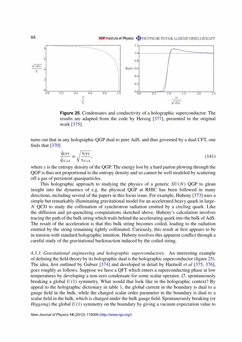
88

0.0 0.2 0.4 0.6 0.8 1.00

2

4

6

8

T

Tc

O

Tc

0.0 0.5 1.0 1.5 2.0 2.50.0

0.2

0.4

0.6

0.8

1.0

1.2

O

Re

Figure 25. Condensates and conductivity of a holographic superconductor. Theresults are adapted from the code by Herzog [377], presented in the originalwork [375].

turns out that in any holographic QGP dual to pure AdS, and thus governed by a dual CFT, onefinds that [370]

qCFT

qN=4=

√sCFT

sN=4, (141)

where s is the entropy density of the QGP. The energy lost by a hard parton plowing through theQGP is thus not proportional to the entropy density and so cannot be well modeled by scatteringoff a gas of persistent quasiparticles.

This holographic approach to studying the physics of a generic SU (N ) QGP to gleaninsight into the dynamics of e.g. the physical QGP at RHIC has been followed in manydirections, including several of the papers in this focus issue. For example, Hubeny [373] uses asimple but remarkably illuminating gravitational model for an accelerated heavy quark in large-N QCD to study the collimation of synchrotron radiation emitted by a circling quark. Likethe diffusion and jet-quenching computations sketched above, Hubeny’s calculation involvestracing the path of the bulk string which trails behind the accelerating quark into the bulk of AdS.The result of the acceleration is that this bulk string becomes coiled, leading to the radiationemitted by the string remaining tightly collimated. Curiously, this result at first appears to bein tension with standard holographic intuition. Hubeny resolves this apparent conflict through acareful study of the gravitational backreaction induced by the coiled string.

4.3.3. Gravitational engineering and holographic superconductors. An interesting exampleof defining the field theory by its holographic dual is the holographic superconductor (figure 25).The idea, first outlined by Gubser [374] and developed in detail by Hartnoll et al [375, 376],goes roughly as follows. Suppose we have a QFT which enters a superconducting phase at lowtemperatures by developing a non-zero condensate for some scalar operator, O, spontaneouslybreaking a global U (1) symmetry. What would that look like in the holographic context? Byappeal to the holographic dictionary in table 1, the global current in the boundary is dual to agauge field in the bulk, while the charged scalar order parameter in the boundary is dual to ascalar field in the bulk, which is charged under the bulk gauge field. Spontaneously breaking (orHiggsing) the global U (1) symmetry on the boundary by giving a vacuum expectation value to

New Journal of Physics 14 (2012) 115009 (http://www.njp.org/)

89

O is then dual to spontaneously breaking the bulk gauge U (1) via a non-trivial profile for thebulk scalar field, 8(r).

Our goal is thus to build a gravitational system which is dual to some QFT which exhibitsthis symmetry breaking pattern—not a specific QFT, but any QFT with this structure. Byadjusting the gravitational theory we will then be able to explore a whole space of stronglycoupled QFTs with low-energy superfluid phases. Procedurally, we will take the gravitationalsystem as a definition of the dual QFT, computing the correlation functions, etc, of the QFTentirely by appeal to the holographic dual.

The holographic dictionary thus tells us that, whatever else exists in the gravitational dualof a superconducting QFT, we will need a vector field Aµ dual to the boundary current Jm anda scalar field 8 dual to the scalar order parameter O. The dictionary, however, does not tell usthe Lagrangian, so we must choose it. A minimal first guess is

Igrav =−1

16πGN

∫√

g

(−23+ R−

1

e2

[1

4F2 + |D8|2 + m2

|8|2]). (142)

We can further simplify our lives by considering the probe limit, g→∞, in which case thematter field stress tensor (which scales as 1

e2 ) is negligible so that the Einstein equation, and thusthe metric, is not modified from its original AdS form.

Our task now is to find non-trivial solutions of the bulk equations of motion which followfrom our trial action expanded around an AdS black brane geometry, so as to put the system atfinite temperature.

Non-trivial means that the scalar field 8 acquires a non-vanishing profile whichspontaneously breaks the gauge symmetry in the bulk. From our dictionary, this correspondsto the boundary operator O acquiring a vacuum expectation value which spontaneously breaksthe global symmetry on the boundary. Once we find such a solution, we can compute correlationfunctions in the resulting system by evaluating the bulk action on-shell as a functional of thenon-normalizable modes and taking derivatives with respect to those modes, as discussed insection 4.2.3.

For simplicity, let us focus on homogeneous configurations of the form A = At(r)dt and8=8(r). The bulk equations of motion in our AdS black brane take the form

r 2 f A′′t − 2|8|2 At = 0, r 2 f 8′′ + (r f ′−2 f )r8′ +

(r 2 A2

t

f−m2

)8= 0. (143)

Near the boundary, the general solution to the bulk field equations takes the form

At ∼ µ + ρ r + · · · , 8∼ φd−1r d−1 +φ1r1 + · · · , (144)

where m2L2=1(1− d). A convenient choice for the mass is m2L2

=−2, which gives 1= 1or 2. Let us focus on 1= 2. The holographic dictionary tells us to interpret µ as the source ofthe Jt component of the current, so µ plays the role of the chemical potential for the boundarycharge density. ρ, being the subleading piece of At near the boundary, then represents theexpectation value of the operator conjugate to µ, ρ = 〈Jt〉, so we can identify ρ as the chargedensity induced by µ. Similarly, φd−1, as the leading term in8 near the boundary, is interpretedas the source for the boundary operator O, and φ1 as the vacuum expectation value, φ1 = 〈O〉.

To construct a spontaneous condensate, we should turn off the source, φd−1 = 0, fix areference value for the chemical potential, µ= µo, and look for a solution of the bulk equations

New Journal of Physics 14 (2012) 115009 (http://www.njp.org/)

90

of motion which have, below some critical temperature Tc, a non-zero value for 〈O〉 = φ1.This requires that we solve equations (143) subject to the boundary conditions that 8(0)= 0(no source) and At(0)= µo. Generally, this must be done numerically, as equations (143) arenonlinearly coupled. By evaluating the on-shell action and using the holographic dictionary intable 1, we can compute physical quantities. For example, we find the critical temperature bysearching for the minimum T of the background black brane such that a non-trivial solution withthese boundary conditions exists. We find the ac conductivities by looking at linear responsefor fluctuations of Ax linearized around a non-trivial solution for At and 8, etc. The precisebehavior we find depends on the details of the gravitational model chosen. By adding additionalfields and interactions, we can use these techniques to engineer a wide range of dynamicalphenomena in the dual QFT.

The point to emphasize here is that while we are explicitly computing correlation functionsin a strongly coupled QFT, and indeed studying the detailed physics of transport, the QFT underinvestigation is defined purely through its gravitational dual. We thus call these superconductorsholographic superconductors, and more generally refer to such QFTs as holographic QFTs.

Importantly, these models can be used to study much more than just the translationallyinvariant ground states of these strongly interacting superfluids. For example, they providea simple and powerful framework for studying spatially ordered phases and solitons. Forexample, the paper by Keranen et al in this focus issue [164] uses solitons in these holographicsuperconductors as precision probes of the superfluid, including, in particular, the excitationspectrum [378, 379] around a dark soliton at unitarity in the BCS–BEC crossover [162,165–167]. As the solution of this problem reduces to a detailed study of coupled PDEs,considerable progress can be made with common computational techniques toward a concreteprediction observable in the present experiments on ultracold quantum gases.

Notably, this holographic mechanism for spontaneously breaking a symmetry can beapplied to any boundary QFT with symmetry breaking. For example, the paper by Basuet al in this focus issue [380] uses the holographic superconductor paradigm to study colorsuperconductivity in holographic models of the QGP. As good effective field theorists, Basu et albegin by writing down a gravitational effective theory with the minimal ingredients to mock upa color superconductor and then examine what constraints they must impose on the parametersof this effective description to reproduce the expected physics of a true color superconductor.

4.3.4. Non-relativistic holography and cold atoms. Strongly correlated quantum liquids ofcold atoms provide an excellent target for applied holography. From a holographic point ofview, cold atoms at unitarity are very similar to N = 4 models of the RHIC fireball: theyprovide examples of strongly correlated liquids at finite temperature and chemical potentialthat are governed by a conformal field theory. The key difference is that these systems are non-relativistic, with dispersion relations scaling as66

ω ∼ kz, (145)

so that the RG fixed points that govern their dynamics are non-relativistic conformal fieldtheories (NRCFTs) [381–383]. Furthermore, in the case z = 2 arising in cold fermions at

66 The scaling exponent z is called the dynamical exponent, and can be extracted either from the dispersion relationfor low-lying modes or from the scaling of the characteristic time scale with the correlation length, τ ∼ ξ z , as weapproach a critical point [340].

New Journal of Physics 14 (2012) 115009 (http://www.njp.org/)

91

unitarity, the symmetry algebra is enlarged [383] and includes a central number operator,N , such that every operator has, in addition to a dimension, 1, a conserved particle numbereigenvalue, N .

Holographically, the non-relativistic scaling has a dramatic effect. In the case of N = 4theory, relativistic conformal invariance was enough to determine the dual space–time, with theconformal symmetry group of the QFT, SO(4, 2), mapping to the isometry group of the dualspace–time; this fixes the geometry dual to the N = 4 theory to be AdS5. More generally, thefact that relativistic QFTs flow to Lorentz-invariant RG fixed points in the UV implies that theirholographic duals should asymptotically approach pure AdS near the boundary. If our QFTdoes not possess Lorentz invariance, the dual space–time cannot be simple AdS. To build theholographic dual of an NRCFT, then, we must start from the beginning and identify the rightspace–time.

The simplest geometry with these properties is the Lifschitz metric [308]

ds2= L2

(−

dt2

r 2z+

dEx2 + dr 2

r 2

). (146)

In this geometry, every slice at a fixed r is again a copy of flat space, but the scaling of the time-like coordinate and the spatial coordinates under a shift in r is inhomogeneous, with scalingω ∼ kz. At z = 1, this reduces precisely to the AdS case, a good check. However, at z = 2 thereis no enhancement of the isometry group of the geometry, so it is natural to look for anothergeometry which realizes the full enhanced z = 2 non-relativistic conformal symmetry group.Following this logic leads to the Schrodinger metric [306, 307]

ds2= L2

(−

dt2

r 2z+

2dt dξ + dEx2 + dr 2

r 2

), (147)

where ξ is a new periodic variable. Again we find that scaling implies that ω ∼ kz. Now,however, the isometry group of the manifold is in fact enhanced at z = 2. Moreover, since ξis compact, we can expand every field in eigenmodes of N = i∂ξ , so that bulk fields, and thus allboundary operators to which they are dual, are labeled by both a dimension, 1, and also aξ -momentum, N . We thus have a geometry which enjoys both of the peculiar features offermions at unitarity identified above.

Repeating the full construction in section 4.2 in this non-relativistic setting remains anopen problem. However, considerable progress has been made in the context of both Lifschitzand Schrodinger systems, including the construction of charged black holes corresponding toNRCFTs at finite temperature and chemical potential [384–387] and the construction of sometoy non-relativistic superfluids (see, e.g., [388] in this focus issue). Many of the basic universalresults from the relativistic setting have been replicated. For example, in the simplest modelswe again find η

s =1

4π . Note that, while we have suppressed factors of c throughout, there areno such factors in this result for the viscosity ratio so we get a non-trivial prediction for non-relativistic systems. Furthermore, while η

s is a natural observable in relativistic QFTs even ifwe do not know about holography (it is the dimensionless momentum diffusion constant inlinearized hydrodynamics), the fact that ηs is relevant in non-relativistic systems is an interestingfeature of holography; the momentum diffusion constant in non-relativistic hydrodynamics is

New Journal of Physics 14 (2012) 115009 (http://www.njp.org/)

92

η

n . In the context of Lifschitz scaling, considerably more progress has been made, includinginteresting results for models of strange metals [389].67

For models of cold atoms, on the other hand, our non-relativistic holographic modelsremain rather distant from the systems studied in actual experiments. Indeed, it seems likelythat fermions at unitarity, like QCD, do not have weakly coupled holographic duals. However,unlike QCD, where we have already built holographic toy models which capture a greatdeal of the strong-coupling phenomena, non-relativistic CFTs with dynamical exponent z = 2and Schrodinger symmetry have proven difficult to model holographically. In particular, thethermodynamics and phase structure of current holographic models are not obviously relatedto any known systems, if not outright pathological [384–386]. For example, we expect thefinite-density ground state of these theories to form a superfluid which spontaneously breaksthe U (1) symmetry generated by the number operator, N . Holographically, N is mappedto ∂ξ , the generator of translations in the second holographic direction. Such a superfluidground state must thus break translation invariance in the ξ -direction. Unfortunately, all ourcurrent holographic models of z = 2 Schrodinger CFTs feature manifest unbroken ξ -translationinvariance.

This problem can be traced [390–392] to the fact that all our current models werederived from highly symmetric stringy systems which enforce this symmetry. As a result, theselimitations do not appear to be intrinsic to the holographic framework but rather to the veryspecific models which have so far been studied. It would be of great interest to develop morerealistic models (see, e.g., [392] for a recent work in this direction). A step in this direction isdescribed in the paper by Adams and Wang in this focus issue [388], in which a superconductingground state for such a non-relativistic holographic CFT is constructed by extending the‘holographic superconductor’ strategy from AdS to these non-relativistic geometries. This leadsto various interesting effects, including a surprising quantum phase transition as the densityof the fluid is varied and a multicritical point where the transition to the superfluid stateswitches from second to first order. This does not solve the underlying problem, as the geometryremains unmodified, but is at least a proof of principle that such holographic ground states doexist.

4.3.5. Holographic non-Fermi liquids and critical phenomena. Fermi surfaces are familiarbeasts, and are generally well described by standard quasiparticle perturbation theory. Thisis true despite the fact that the electrons living on the Fermi surface may interact throughthe infinite-range Coulomb potential. The key point is that the phase space available for twoelectrons to scatter is extremely limited, as both the initial electron states and the final electronstates must all lie on the Fermi surface. Folding in this phase space constraint, the effectiveinteraction for (dressed) electrons scattering on the spherical Fermi surface mediated by the

67 It is worth emphasizing that it is straightforward to build holographic models in which the dynamical exponentchanges as the theory flows from the UV to IR. A particularly illuminating example involves the fate of chargedblack holes with large ground-state degeneracies. In at least some holographic models it has been shown that theground state degeneracy is lifted by a dynamical instability which changes the near-horizon geometry from AdS toLifschitz geometries which have no, or at least vastly diminished, ground state degeneracy. Since the near-horizonregion encodes the IR physics of the dual QFT, such holographic models describe QFTs where the dynamicalexponent of the low-energy degrees of freedom arises due to strong interactions among constituents with no simplequasiparticle description, and is thus effectively invisible in the UV regime. The dynamical scaling is in this senseemergent.

New Journal of Physics 14 (2012) 115009 (http://www.njp.org/)

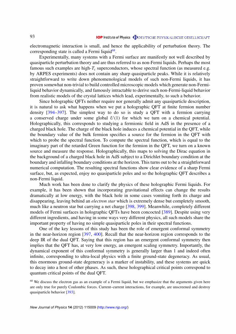
93

electromagnetic interaction is small, and hence the applicability of perturbation theory. Thecorresponding state is called a Fermi liquid68.

Experimentally, many systems with a Fermi surface are manifestly not well described byquasiparticle perturbation theory and are thus referred to as non-Fermi liquids. Perhaps the mostfamous such examples are high-Tc superconductors, whose spectral function (as measured e.g.by ARPES experiments) does not contain any sharp quasiparticle peaks. While it is relativelystraightforward to write down phenomenological models of such non-Fermi liquids, it hasproven somewhat non-trivial to build controlled microscopic models which generate non-Fermi-liquid behavior dynamically, and famously intractable to derive such non-Fermi-liquid behaviorfrom realistic models of the crystal lattices which lead, experimentally, to such a behavior.

Since holographic QFTs neither require nor generally admit any quasiparticle description,it is natural to ask what happens when we put a holographic QFT at finite fermion numberdensity [394–397]. The simplest way to do so is study a QFT with a fermion carryinga conserved charge under some global U (1) for which we turn on a chemical potential.Holographically, this corresponds to studying a fermionic field in AdS in the presence of acharged black hole. The charge of the black hole induces a chemical potential in the QFT, whilethe boundary value of the bulk fermion specifies a source for the fermion in the QFT withwhich to probe the spectral function. To compute the spectral function, which is equal to theimaginary part of the retarded Green function for the fermion in the QFT, we turn on a knownsource and measure the response. Holographically, this maps to solving the Dirac equation inthe background of a charged black hole in AdS subject to a Dirichlet boundary condition at theboundary and infalling boundary conditions at the horizon. This turns out to be a straightforwardnumerical computation. The resulting spectral functions show clear evidence of a sharp Fermisurface, but, as expected, enjoy no quasiparticle poles and so the holographic QFT describes anon-Fermi liquid.

Much work has been done to clarify the physics of these holographic Fermi liquids. Forexample, it has been shown that incorporating gravitational effects can change the resultsdramatically at low energy, with the black hole in some cases vomiting forth its charge anddisappearing, leaving behind an electron star which is extremely dense but completely smooth,much like a neutron star but carrying a net charge [398, 399]. Meanwhile, completely differentmodels of Fermi surfaces in holographic QFTs have been concocted [389]. Despite using verydifferent ingredients, and having in some ways very different physics, all such models share theimportant property of having no simple quasiparticle poles in their spectral functions.

One of the key lessons of this study has been the role of emergent conformal symmetryin the near-horizon region [397, 400]. Recall that the near-horizon region corresponds to thedeep IR of the dual QFT. Saying that this region has an emergent conformal symmetry thenimplies that the QFT has, at very low energy, an emergent scaling symmetry. Importantly, thedynamical exponent of this conformal symmetry is generally larger than 1 and indeed ofteninfinite, corresponding to ultra-local physics with a finite ground-state degeneracy. As usual,this enormous ground-state degeneracy is a marker of instability, and these systems are quickto decay into a host of other phases. As such, these holographical critical points correspond toquantum critical points of the dual QFT.

68 We discuss the electron gas as an example of a Fermi liquid, but we emphasize that the arguments given hereare only true for purely Coulombic forces. Current–current interactions, for example, are unscreened and destroyquasiparticle behavior [393].

New Journal of Physics 14 (2012) 115009 (http://www.njp.org/)

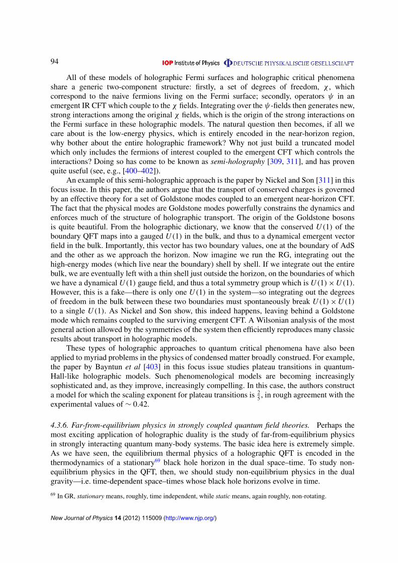
94

All of these models of holographic Fermi surfaces and holographic critical phenomenashare a generic two-component structure: firstly, a set of degrees of freedom, χ , whichcorrespond to the naive fermions living on the Fermi surface; secondly, operators ψ in anemergent IR CFT which couple to the χ fields. Integrating over the ψ-fields then generates new,strong interactions among the original χ fields, which is the origin of the strong interactions onthe Fermi surface in these holographic models. The natural question then becomes, if all wecare about is the low-energy physics, which is entirely encoded in the near-horizon region,why bother about the entire holographic framework? Why not just build a truncated modelwhich only includes the fermions of interest coupled to the emergent CFT which controls theinteractions? Doing so has come to be known as semi-holography [309, 311], and has provenquite useful (see, e.g., [400–402]).

An example of this semi-holographic approach is the paper by Nickel and Son [311] in thisfocus issue. In this paper, the authors argue that the transport of conserved charges is governedby an effective theory for a set of Goldstone modes coupled to an emergent near-horizon CFT.The fact that the physical modes are Goldstone modes powerfully constrains the dynamics andenforces much of the structure of holographic transport. The origin of the Goldstone bosonsis quite beautiful. From the holographic dictionary, we know that the conserved U (1) of theboundary QFT maps into a gauged U (1) in the bulk, and thus to a dynamical emergent vectorfield in the bulk. Importantly, this vector has two boundary values, one at the boundary of AdSand the other as we approach the horizon. Now imagine we run the RG, integrating out thehigh-energy modes (which live near the boundary) shell by shell. If we integrate out the entirebulk, we are eventually left with a thin shell just outside the horizon, on the boundaries of whichwe have a dynamical U (1) gauge field, and thus a total symmetry group which is U (1)×U (1).However, this is a fake—there is only one U (1) in the system—so integrating out the degreesof freedom in the bulk between these two boundaries must spontaneously break U (1)×U (1)to a single U (1). As Nickel and Son show, this indeed happens, leaving behind a Goldstonemode which remains coupled to the surviving emergent CFT. A Wilsonian analysis of the mostgeneral action allowed by the symmetries of the system then efficiently reproduces many classicresults about transport in holographic models.

These types of holographic approaches to quantum critical phenomena have also beenapplied to myriad problems in the physics of condensed matter broadly construed. For example,the paper by Bayntun et al [403] in this focus issue studies plateau transitions in quantum-Hall-like holographic models. Such phenomenological models are becoming increasinglysophisticated and, as they improve, increasingly compelling. In this case, the authors constructa model for which the scaling exponent for plateau transitions is 2

5 , in rough agreement with theexperimental values of ∼ 0.42.

4.3.6. Far-from-equilibrium physics in strongly coupled quantum field theories. Perhaps themost exciting application of holographic duality is the study of far-from-equilibrium physicsin strongly interacting quantum many-body systems. The basic idea here is extremely simple.As we have seen, the equilibrium thermal physics of a holographic QFT is encoded in thethermodynamics of a stationary69 black hole horizon in the dual space–time. To study non-equilibrium physics in the QFT, then, we should study non-equilibrium physics in the dualgravity—i.e. time-dependent space–times whose black hole horizons evolve in time.

69 In GR, stationary means, roughly, time independent, while static means, again roughly, non-rotating.

New Journal of Physics 14 (2012) 115009 (http://www.njp.org/)

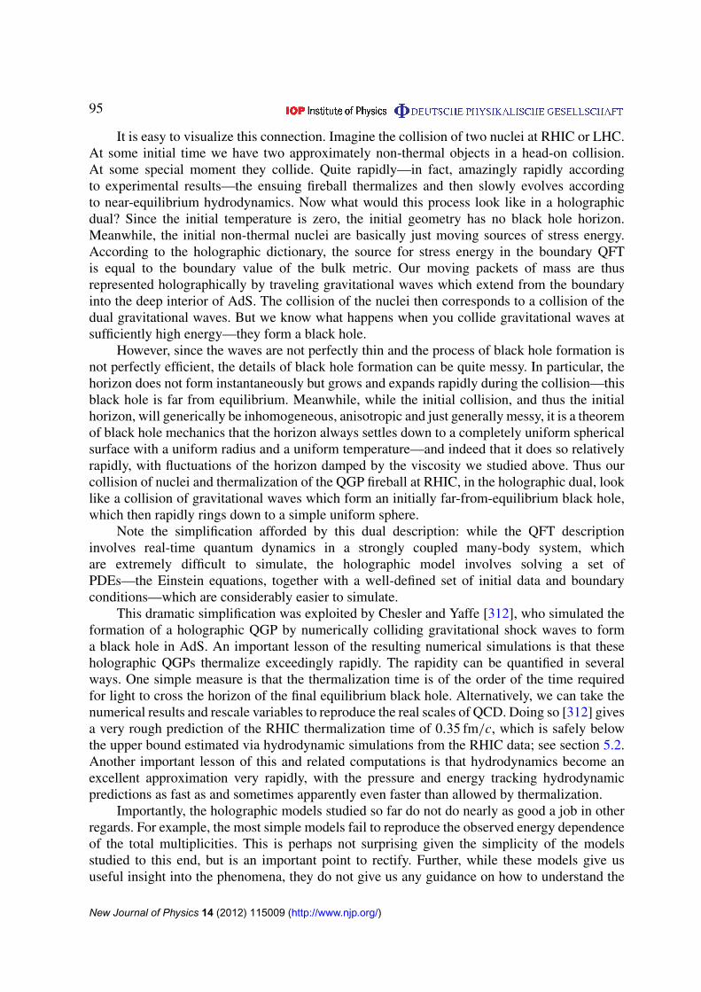
95

It is easy to visualize this connection. Imagine the collision of two nuclei at RHIC or LHC.At some initial time we have two approximately non-thermal objects in a head-on collision.At some special moment they collide. Quite rapidly—in fact, amazingly rapidly accordingto experimental results—the ensuing fireball thermalizes and then slowly evolves accordingto near-equilibrium hydrodynamics. Now what would this process look like in a holographicdual? Since the initial temperature is zero, the initial geometry has no black hole horizon.Meanwhile, the initial non-thermal nuclei are basically just moving sources of stress energy.According to the holographic dictionary, the source for stress energy in the boundary QFTis equal to the boundary value of the bulk metric. Our moving packets of mass are thusrepresented holographically by traveling gravitational waves which extend from the boundaryinto the deep interior of AdS. The collision of the nuclei then corresponds to a collision of thedual gravitational waves. But we know what happens when you collide gravitational waves atsufficiently high energy—they form a black hole.

However, since the waves are not perfectly thin and the process of black hole formation isnot perfectly efficient, the details of black hole formation can be quite messy. In particular, thehorizon does not form instantaneously but grows and expands rapidly during the collision—thisblack hole is far from equilibrium. Meanwhile, while the initial collision, and thus the initialhorizon, will generically be inhomogeneous, anisotropic and just generally messy, it is a theoremof black hole mechanics that the horizon always settles down to a completely uniform sphericalsurface with a uniform radius and a uniform temperature—and indeed that it does so relativelyrapidly, with fluctuations of the horizon damped by the viscosity we studied above. Thus ourcollision of nuclei and thermalization of the QGP fireball at RHIC, in the holographic dual, looklike a collision of gravitational waves which form an initially far-from-equilibrium black hole,which then rapidly rings down to a simple uniform sphere.

Note the simplification afforded by this dual description: while the QFT descriptioninvolves real-time quantum dynamics in a strongly coupled many-body system, whichare extremely difficult to simulate, the holographic model involves solving a set ofPDEs—the Einstein equations, together with a well-defined set of initial data and boundaryconditions—which are considerably easier to simulate.

This dramatic simplification was exploited by Chesler and Yaffe [312], who simulated theformation of a holographic QGP by numerically colliding gravitational shock waves to forma black hole in AdS. An important lesson of the resulting numerical simulations is that theseholographic QGPs thermalize exceedingly rapidly. The rapidity can be quantified in severalways. One simple measure is that the thermalization time is of the order of the time requiredfor light to cross the horizon of the final equilibrium black hole. Alternatively, we can take thenumerical results and rescale variables to reproduce the real scales of QCD. Doing so [312] givesa very rough prediction of the RHIC thermalization time of 0.35 fm/c, which is safely belowthe upper bound estimated via hydrodynamic simulations from the RHIC data; see section 5.2.Another important lesson of this and related computations is that hydrodynamics become anexcellent approximation very rapidly, with the pressure and energy tracking hydrodynamicpredictions as fast as and sometimes apparently even faster than allowed by thermalization.

Importantly, the holographic models studied so far do not do nearly as good a job in otherregards. For example, the most simple models fail to reproduce the observed energy dependenceof the total multiplicities. This is perhaps not surprising given the simplicity of the modelsstudied to this end, but is an important point to rectify. Further, while these models give ususeful insight into the phenomena, they do not give us any guidance on how to understand the

New Journal of Physics 14 (2012) 115009 (http://www.njp.org/)

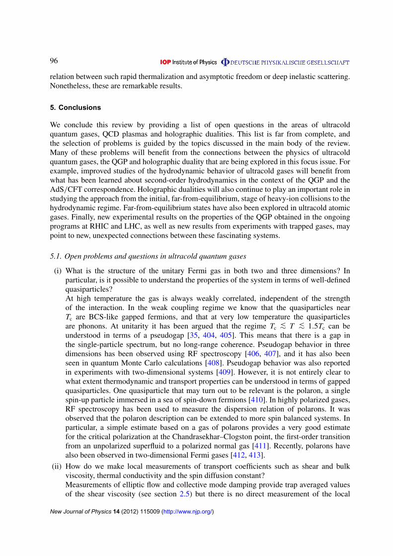
96

relation between such rapid thermalization and asymptotic freedom or deep inelastic scattering.Nonetheless, these are remarkable results.

5. Conclusions

We conclude this review by providing a list of open questions in the areas of ultracoldquantum gases, QCD plasmas and holographic dualities. This list is far from complete, andthe selection of problems is guided by the topics discussed in the main body of the review.Many of these problems will benefit from the connections between the physics of ultracoldquantum gases, the QGP and holographic duality that are being explored in this focus issue. Forexample, improved studies of the hydrodynamic behavior of ultracold gases will benefit fromwhat has been learned about second-order hydrodynamics in the context of the QGP and theAdS/CFT correspondence. Holographic dualities will also continue to play an important role instudying the approach from the initial, far-from-equilibrium, stage of heavy-ion collisions to thehydrodynamic regime. Far-from-equilibrium states have also been explored in ultracold atomicgases. Finally, new experimental results on the properties of the QGP obtained in the ongoingprograms at RHIC and LHC, as well as new results from experiments with trapped gases, maypoint to new, unexpected connections between these fascinating systems.

5.1. Open problems and questions in ultracold quantum gases

(i) What is the structure of the unitary Fermi gas in both two and three dimensions? Inparticular, is it possible to understand the properties of the system in terms of well-definedquasiparticles?At high temperature the gas is always weakly correlated, independent of the strengthof the interaction. In the weak coupling regime we know that the quasiparticles nearTc are BCS-like gapped fermions, and that at very low temperature the quasiparticlesare phonons. At unitarity it has been argued that the regime Tc

<∼ T <

∼ 1.5Tc can beunderstood in terms of a pseudogap [35, 404, 405]. This means that there is a gap inthe single-particle spectrum, but no long-range coherence. Pseudogap behavior in threedimensions has been observed using RF spectroscopy [406, 407], and it has also beenseen in quantum Monte Carlo calculations [408]. Pseudogap behavior was also reportedin experiments with two-dimensional systems [409]. However, it is not entirely clear towhat extent thermodynamic and transport properties can be understood in terms of gappedquasiparticles. One quasiparticle that may turn out to be relevant is the polaron, a singlespin-up particle immersed in a sea of spin-down fermions [410]. In highly polarized gases,RF spectroscopy has been used to measure the dispersion relation of polarons. It wasobserved that the polaron description can be extended to more spin balanced systems. Inparticular, a simple estimate based on a gas of polarons provides a very good estimatefor the critical polarization at the Chandrasekhar–Clogston point, the first-order transitionfrom an unpolarized superfluid to a polarized normal gas [411]. Recently, polarons havealso been observed in two-dimensional Fermi gases [412, 413].

(ii) How do we make local measurements of transport coefficients such as shear and bulkviscosity, thermal conductivity and the spin diffusion constant?Measurements of elliptic flow and collective mode damping provide trap averaged valuesof the shear viscosity (see section 2.5) but there is no direct measurement of the local

New Journal of Physics 14 (2012) 115009 (http://www.njp.org/)

97

value of the shear viscosity η(n, T ). The status is roughly analogous to the situation afterthe first experiments aimed at measuring the equation of state. These experiments onlydetermined the total energy and entropy [66]. Local measurements were made possibleby new ideas such as the Gibbs–Duhem method employed by the ENS group [68] andthe compressibility thermometer introduced by the MIT group [36]. It is possible, inprinciple, to unfold the currently available data for trap averaged viscosities, but thismethod requires a very careful treatment of the dilute corona, and a more direct methodwould be desirable. One possible direction is the development of new experimentaltechniques that generate local shear flows and study their relaxation. Another option is tomeasure the frequency-dependent shear viscosity via spectroscopic methods as suggestedin [414]. Similar questions apply to other transport properties, such as bulk viscosity,thermal conductivity and spin diffusion. Current methods are mostly sensitive to averagetransport coefficients, but more local measurements are needed.

(iii) Are there reliable approaches to transport theory beyond the Boltzmann equation?In the unitary limit, transport properties can be computed reliably using the Boltzmannequation in the limit T � TF. For T ∼ TF the quasiparticles are strongly interacting, andthe kinetic description in terms of binary scattering between atoms breaks down. Ensset al [129] have computed the shear viscosity using a T -matrix resummation. A similarapproach is discussed by Guo et al [110] in this focus issue. These methods are quitesuccessful in describing the thermodynamics, but there is no expansion parameter, andit is not clear if non-equilibrium properties are predicted as well as equilibrium features.In section 2.2 we briefly discuss the application of 1/N and ε expansions to equilibriumproperties of the unitary gas, but except for the recent work of [415] these methods havenot been extended to non-equilibrium properties. Similar remarks apply to other methodsas well: there are detailed studies of equilibrium properties using the exact RG [416], butno corresponding studies of transport properties. Finally, there now exist very accuratequantum Monte Carlo calculations of the equation of state, but there is only a single,pioneering, study of transport properties [5].

(iv) Are there other universal quantum gases that can be created by manipulating thedimensionality, the spin structure, the type of interaction or the dispersion relation?The unitary gas exhibits a very high degree of universality: in the limit of infinite scatteringlength and zero effective range the many-body system is completely characterized bythe fermion mass, the temperature and the chemical potential. The dependence ondimensionful combinations of these parameters is completely governed by dimensionalanalysis. Universality can be exploited to use the unitary gas as a model system for diluteneutron matter; see section 3.1. The question is whether this idea can be extended tomore complicated systems, for example three-species gases that can serve as a modelfor the quark matter/nuclear matter transition (see section 2.7) or four-species gases thatcorrespond to self-bound nuclear matter, which is a liquid of equal numbers of spin-upand -down protons and neutrons. Universality in systems with more than two degrees offreedom is more complicated, because the interaction depends also on at least one three-body parameter [417], and the system may require repulsive short-range forces in order toprevent collapse. New universal states can also be created by combining Bose and Fermigases in different dimensions [418] or by manipulating the dispersion relation of the atoms.Steps in this direction were recently taken by Salger et al [419], who demonstrated lineardispersion and Klein tunneling of a Bose–Einstein condensate in a 1D optical lattice,

New Journal of Physics 14 (2012) 115009 (http://www.njp.org/)

98

and by Taruell et al [420], who created a two-dimensional optical lattice with the samehoneycomb lattice structure as graphene and therefore obtained low-energy fermions witha linear dispersion relation.

(v) What is the physics of the crossover in the discrete context of optical lattices?Will the predictions of holographic duality of a lower limit on the ratio of viscosity toentropy hold true in the lattice context or not? What class of theories from holographicduality might map onto the Fermi resonance Hamiltonian or other effective two-channelmodels? How can we extend such models to treat the imbalanced Fermi gas? How will apolaron gas be described in the lattice context?

(vi) What will be the interplay between disorder and interactions for the unitary gas?The relative effects of disorder and interactions on both thermal and quantum phasetransitions in quantum many-body physics are an open question generally (see, e.g., [421]).An essential feature of disorder is Anderson localization, in which scattering off of manysmall defects conspires to localize all states above a certain threshold in three dimensions.This concept is, in fact, a wave physics or single-particle quantum concept: it has beenso far unclear where and how interactions destroy or allow for Anderson localizationin a generic sense. Disorder was treated in this focus issue for ultracold Fermi gasesspecifically by Han and Sa de Melo [172]. Here, too, we find potential connections toholographic duality, as explored in recent forays into disordered systems by Adams andYaida [422, 423]. Although these explorations have not treated lattice physics in particular,disorder is an essential feature of lattice systems arising in nature, and can be inducedartificially in various ways for optical lattices [424]. Can holographic duality capture theunderlying lattice causes of disorder? How will experiments in ultracold Fermi gasescombine disordered optical lattices with unitary fermions at sufficiently low temperatures?Might studies in this direction help us gain some fundamental insight into the interplaybetween disorder and interactions in strongly correlated systems?

5.2. Open problems and questions in quantum chromodynamic plasmas

(i) Can we determine all the transport properties of the QGP?We would like to determine, with fully quantified experimental and theoreticaluncertainties, the value of the shear viscosity to entropy density ratio η/s, the heavy quarkdiffusion constant D and the jet quenching parameter q. This program is probably closestto completion in the case of η/s. In this case the basic method, second-order relativisticviscous hydrodynamics, is now fairly well understood. Final state corrections can behandled by coupling to a hadronic cascade. There is a large set of data, including the energy,impact parameter and system size dependence of elliptic flow, as well as the observation ofhigher harmonics that points to the validity of the hydrodynamic description. The internalconsistency of hydrodynamics already implies a fairly strong bound η/s <∼ 0.5–1.0. Themain problem is that we have no direct method for establishing the initial conditions forthe hydrodynamic description. This problem may be addressed by focusing on a larger setof observables, in particular higher harmonics of the flow [425, 426]. There also remaintheoretical uncertainties regarding the coupling of viscous fluid dynamics to a Boltzmanndescription, the role of bulk viscosity and the equation of state. A discussion of the knownuncertainties in η/s can be found in [427].

The main strategy for determining the heavy quark diffusion constant is to use aLangevin description of the diffusion process where the background collective expansion

New Journal of Physics 14 (2012) 115009 (http://www.njp.org/)

99

is taken from hydrodynamics. The most important problem at present is the fact that thereare only data for single leptons, and not for identified heavy quarks. This problem will besolved by improved detection capabilities at RHIC and LHC. The main theoretical issue ishow to handle the interplay between elastic and inelastic scattering. For very heavy quarkselastic scattering is dominant, but for charm quarks inelastic processes may be important.This includes hadronization effects such as coalescence.

In the case of jet energy loss there are still a number of theoretical issues that need tobe resolved. The radiative energy loss of an energetic parton (E � T ) in a partonic mediumcan be expressed in terms of a single medium parameter, the transverse diffusion constantq. It is not clear if this carries over to the spectra of jets or leading particles producedin the medium. Another source of uncertainty is that different implementations of the in-medium radiation in perturbative QCD lead to significantly different values of q whenapplied to the RHIC data [278]. There is a significant ongoing effort to understand thesedifferences70. On the experimental side, the LHC represents a large step toward higherjet energies E ∼ 100 GeV, and significantly improved statistics in the range E <

∼ 20 GeValready explored at RHIC. Both at the LHC and at RHIC, experimentalists are studying notonly spectra of hard particles, but also identified jets, jet shapes and correlations betweenhard particles and the associated soft emission.

(ii) Can we understand early thermalization?The success of the hydrodynamic description implies that the system must thermalize early.The question is: how to quantify this statement experimentally, and how to understandearly equilibration theoretically? The most reliable constraint on the thermalization timearises from the observation of elliptic flow. Elliptic flow is driven by the anisotropy of theinitial state. Since ballistic expansion dilutes the initial anisotropy, local equilibration musthappen early for elliptic flow to develop. A very conservative constraint, discussed in [182],is τ0 < 2.5 fm/c. Typical values used in hydrodynamic fits are τ0

<∼ 1 fm/c−1. Another hint

of early thermalization comes from the observation of thermal photons with temperaturessignificantly larger than those seen in hadronic spectra. The PHENIX collaboration hasrecently reported a photon transverse momentum spectrum with a slope parameter T =221± 19± 19 MeV [428]. The spectra can be reproduced in hydrodynamic calculationswith thermalization times ranging from τ0

<∼ 0.15 fm/c to τ0

<∼ 0.6 fm/c, corresponding

to initial temperatures T0 ∼ 300–600 MeV. Establishing experimental constraints on theequilibration time is further complicated by the fact that not all observables require fullthermalization. For example, for the development of radial and elliptic flow it is notnecessary that longitudinal momentum distributions be fully equilibrated [429].

Understanding thermalization theoretically is difficult even if the early evolution isgoverned by weak coupling. The first attempt to understand thermalization starting froman initial color-glass state using 2→ 2 and 2→ 3 scattering is the bottom-up scenariodescribed in [430]. It was later realized that this picture is modified by collective effectsthat lead to plasma instabilities [431–433]; see also the contribution by Dusling in thisfocus issue [434]. In all these approaches it is hard to understand how thermalization atRHIC can occur on a time scale τ0

<∼ 1 fm/c.

Attempts to understand thermalization at strong coupling have focused on holographicduality; see section 4.3.6 and [435, 436] for recent overviews. Holographic duality providesan interesting geometric picture of thermalization: the initial state corresponds to two

70 Topical Collaboration on Jet and Electromagnetic Tomography, http://jet.lbl.gov/.

New Journal of Physics 14 (2012) 115009 (http://www.njp.org/)

100

colliding shock waves, and thermalization is signaled by the formation of an event horizon.The hydrodynamic stage is described by the relaxation or ringdown of the black hole. Inholographic duality one can achieve fast equilibration [312], but it is hard to make contactwith asymptotic freedom and the well-established theory and phenomenology of nucleardeep inelastic scattering, and it is difficult to understand the observed energy and impactparameter dependence of the total multiplicity [437].

(iii) Does the QGP have a quasiparticle description?We would like to understand how the properties of the hot and dense matter producedat RHIC and the LHC are related to its structure, in particular whether the matter canindeed be described as a plasma made of quarks and gluons. Holographic duality seemto indicate that a strongly interacting quantum fluid near the viscosity bound does nothave a quasiparticle description; see sections 3.2 and 4. In section 3.2 we discussed anumber of observables that have been suggested as probes of the quasiparticle structure:fluctuations, the observed constituent quark scaling of flow, and the relation between theheavy quark diffusion constant and the shear viscosity. None of these observables providesa conclusive test of the quasiparticle picture, and new ideas would certainly be helpful. Wealso discussed the possibility to study quasiparticles by extracting the spectral functions ofthe correlators of conserved charges in lattice QCD, such as energy, momentum, flavor, etc.These studies, too, are somewhat indirect, because on the lattice we only have direct accessto imaginary time correlation functions. This means that the spectral functions have to beextracted via analytic continuation. Analytic continuation of numerical data is difficult, butthere has been significant progress over the last couple of years [438].

(iv) Can we experimentally locate the phase transition?There is a continuing effort to establish the presence of a critical endpoint in the QCDphase diagram. The basic idea is to look for the non-monotonic behavior of fluctuationsor correlations as a function of the energy of the colliding system. The first data fromthe RHIC beam energy scan have recently been released [439]; see also the contribution byMohanty [440] in this focus issue. The data contain new information about the beam energydependence of hydrodynamic flow which will help to establish the onset of a nearly perfectfluidity. Gupta et al [214] have argued that data on fluctuations can be directly comparedwith lattice QCD and that it can be used to set the scale for the phase transition at zerochemical potential. There is not yet conclusive evidence for the existence of a critical point,but data for additional beam energies and with better statistics will become available in thenear future. In heavy-ion collisions the growth of the correlation length is limited by finitesize and finite time effects, and it is important to identify observables that provide the bestsensitivity to critical behavior. Observables that have been considered include fluctuationsof conserved charges, such as baryon number, other fluctuation observables, such as thepion-to-kaon ratio, the mean pT, or elliptic flow, and higher moments such as skewnessand curtosis [441]. There is a parallel effort to locate the critical endpoint in lattice QCD.This effort is complicated by the sign problem that affects lattice calculations for fermionsat finite chemical potential [442].

The discovery of a critical point would establish the presence of a phase transitionbetween hadronic matter and the QGP. At small chemical potential this transition isonly a crossover. One might hope that it would be possible to detect the crossoverthrough hydrodynamic effects associated with the minimum in the speed of sound nearthe crossover temperature [443]. However, explicit calculations seem to show that there

New Journal of Physics 14 (2012) 115009 (http://www.njp.org/)

101

is no direct link between the presence of a minimum in the speed of sound and the beamenergy dependence of multiplicity and flow [182].

Finally, we would like to demonstrate the existence of quark matter at high densityand low temperature. It is not known whether the cores of compact stars are sufficientlydense to contain quark matter or other exotic phases. The presence of quark matter canbe potentially detected through its effect on the equation of state, which is reflected in themass–radius relationship. There is a very active program to pin down this relationship usingobservations of compact stars [444, 445]. Once the presence of a high-density phase hasbeen established, more detailed information regarding its properties can be derived usingthe cooling and spin-down behavior of compact stars.

5.3. Open problems and questions in holographic duality

(i) What does it take to derive a holographic duality?We have no first-principles derivation of holographic duality. This is perhaps not surprising,since it is a strong–weak duality, but it is frustrating. We do have a number of heuristicarguments, such as those that appeared in section 4.1. We also know how to derive a longbut finite list of dual pairs as decoupling limits of particular string theories, e.g. the originalconstruction, N = 4 Yang–Mills in 4D. But we do not know how to derive the dualitydirectly within the bulk or boundary theories71.

This is important for two main reasons. Firstly, we do not have a thoroughunderstanding of the consistency conditions or regimes of validity of our holographicdual descriptions. We do have general rules of thumb, such as the scalings discussed insection 4.2.3, and we can check for self-consistency in specific examples. But particularlywhen we are defining a QFT via the holographic prescription, it is not always obvious whatthe precise regime of validity is and to what extent we should trust the chosen gravitationaltruncation.

Secondly, if we want to generalize holographic duality, it would be very helpfulto know why it is true in the more familiar examples. For instance, we would like togeneralize to intrinsically anisotropic systems, to asymptotically flat or positive-curvature(dS) space–times or even to understand why this is not possible.

(ii) Given a QFT, what is the gravitational dual?Even if a general derivation is not possible, it would be useful to have a constructive mapwhich allowed us to take an arbitrary QFT and identify the appropriate gravitational dual.For example, what is the exact dual of QCD, not QCD plus a collection of exotic fields,not of large N QCD, not of some toy model, but pure QCD? Similarly, with an eye towardultracold atoms, what is the gravitational dual of the Hubbard model, or of the Kondoproblem?

Again, the fact that holography is a strong–weak duality should give us pause. Aswe have seen, when the gravitational system is weakly coupled, the dual QFT genericallydoes not have any simple quasiparticle interpretation. If we want to define the QFT usingconventional Lagrangian methods, the best we will, in general, be able to do is say that it isthe strong-coupling limit of some explicit perturbative theory. In the models we understandbest, the coupling that is getting strong is tightly constrained by symmetries, e.g. gaugesymmetries, flavor symmetries or supersymmetry, so we know how to follow the RG flow

71 This is not for lack of trying; see [333, 446, 447] for recent approaches.

New Journal of Physics 14 (2012) 115009 (http://www.njp.org/)

102

well beyond the perturbative, quasiparticle regime. We do not know how to solve the moregeneral case without these extraordinary symmetries and the constraints they imply.

(iii) Can we derive gravity from field theory?The holographic graviton looks very much like an emergent vector boson in morefamiliar condensed matter systems. It arises as an emergent dynamical gauge field whichreorganizes the strongly coupled physics into a set of perturbative local fluctuations.However, in holography the graviton (a) lives in one higher dimension and (b)couples universally. Point (a) fits naturally with a basic feature of gravity: since gaugetransformations are coordinate transformations, there can be no truly local degrees offreedom, so any emergent graviton must come along with an emergent space–timedimension with which to fix its gauge redundancy, much as any emergent vector bosonmust come along with an extra Hubbard–Stratanovich scalar to fix its gauge redundancy.This was, in fact, the origin of the term holography in gravitational physics. Point (b) ismore spectacular from the point of view of emergence, but is in fact a necessary feature ofany theory with a fluctuating spin-2 gauge field.

It is thus tempting to wonder whether we can, in fact, derive the graviton in a generalspace–time as an emergent gauge boson in a strongly interacting QFT. Some progress hasbeen made on this front (cf [446]), but a detailed understanding remains elusive.

(iv) Do we always need the complete holographic description?In many of the examples discussed above, and indeed almost generically in the holographicliterature, most of the work is being done by a very small fraction of the total degrees offreedom in the holographic description. For example, in the computation of η/s in N = 4SYM, whose holographic dual, string theory in AdS5× S5, includes an infinite number ofdynamical massive fields, the only fields that matter in the computation are the 5D metricand a single scalar mode encoding one particular fluctuation of this metric. In practice,keeping track of the full holographic description often seems to be overkill72.

This raises two natural questions. Firstly, when does it make sense to truncatethe full holographic description to a small subset of modes? Secondly, might thistruncated holographic model have a more straightforward QFT representation than the fullholographic description? Said differently, might there be a ‘semi-holographic’ formalismdefined entirely within field theory which allows us to build conventional QFTs thatreproduce the interesting phenomenology of fully holographic QFTs without using higherdimensions?

Recent work on holographic Fermi liquids, holographic quantum critical points andholographic quantum liquids (see [309] and especially the work of Nickel and Son in thisfocus issue [311]) demonstrates that at least some of the interesting holographic effectscan indeed be realized in a purely quantum field theoretic formalism. On the other hand,

72 Note that this is analogously true in many-body physics: to describe ground states and low-energy dynamics,one generally only needs a tiny corner of Hilbert space. However, in the holographic description the physics ofa single bulk field represents an enormously complicated and non-local set of interactions among the boundarydegrees of freedom. So, observing that the bulk description can be effectively simplified to a small subset of bulkfields does not immediately imply that the same is true of the boundary QFT. For example, in holographic modelsof non-Fermi liquids, the bulk physics can be truncated rather dramatically, but the dual QFT has no quasiparticledescription and so has not proven amenable to any simple truncation; concretely, the spectral function does not havequasiparticle poles. With that said, it seems worthwhile to search for relations between known effective truncationsin quantum many-body and holographic models.

New Journal of Physics 14 (2012) 115009 (http://www.njp.org/)

103

for questions where the nonlinear dynamics of the geometry such as far-from-equilibriumphysics, as opposed to kinematics or linear response, are important, it seems unlikely thatany semi-holographic description can usefully capture the salient physics. Just how far asemi-holographic approach can be pushed, then, is an extremely interesting question.

(v) What predictions do holography make for generic strongly coupled systems?Once we let go of the idea that our models must be defined by traditional quasiparticleeffective QFTs, we can start asking general questions about the strongly coupled QFTsilluminated by our holographic examples. What common properties do these theoriesshare? What general lessons can we draw about their kinematics, dynamics, phasestructures, critical behavior, equilibration, etc? For example, we already know to expectnearly inviscid hydrodynamic behavior at finite density and low temperature. What elseshould we expect in general? Perhaps most importantly, what lessons can we draw forsystems we really care about?

(vi) What is the holographic dual of a non-relativistic QFT?As discussed in section 4.3.4, non-trivial progress has been made in the study of non-relativistic QFTs and many-body systems. This has led to some simple heuristic lessons,for example that we should expect the viscosity to entropy ratio to again be extremely lowand that the Bertsch parameter73 should be expected to be of the order of unity and remainrelatively insensitive to the coupling constant near strong coupling. However, the state ofcurrent models is rather poor, with awkward thermodynamics and bizarre phase structure.What are we missing? Can we build a holographic dual in the same universality class asfermions at unitarity?

(vii) How (and why) is quantum information encoded in the bulk geometry?Holographically, information about the thermodynamic state of the boundary QFT isencoded in the detailed geometry and matter field backgrounds of the bulk theory. Forexample, the temperature and chemical potential are encoded in the mass and charge ofthe bulk black hole. Similarly, when the QFT is in a pure state, the bulk geometry shouldencode the quantum correlations of the boundary QFT at zero temperature. But how?

One approach to this question is the Ryu–Takanayagi conjecture [448, 449], whichstates that the entanglement entropy associated with a region R in a holographic QFT isgiven by the area of the minimal-area surface in the bulk which ends at the boundaryof the region R. Holographically, this conjecture matches the relation between thethermodynamic entropy of a black hole and the area of its horizon. Interestingly, it suggestsan intimate connection between quantum and thermal entropy—and more generally,between quantum and thermal fluctuations—all of which are encoded by the physics ofhorizons in the holographic dual.

While a general proof is still lacking, considerable evidence has been found for thisconjecture, and conversely, numerous predictions have been made for the entanglemententropy of strongly coupled many-body systems by exploiting this conjecture (see,e.g., [450–455] and references therein). For example, in this focus issue, Albash andJohnson [456] have studied the evolution of the Ryu–Takanayagi entropy under a thermalquench, leading both to evidence supporting the conjecture and to predictions on theevolution of the entanglement entropy.

73 We defined the Bertsch parameter of the unitary Fermi gas in section 2.2. Here we use the term to refer to theratio of the ground-state energy at strong coupling to that at weak coupling in a general non-relativistic CFT.

New Journal of Physics 14 (2012) 115009 (http://www.njp.org/)

104

(viii) How does spatial inhomogeneity change the story?As we have seen, holography translates quantum computations in the boundary QFT (i.e.Feynman diagrams and path integrals) into classical GR calculations in the bulk (i.e.solving nonlinear partial differential equation boundary value problems). As such, it is clearwhy most research to date has focused on homogeneous, isotropic problems. However,on the quantum many-body side, we know that inhomogeneity can radically alter thedynamics, and that the precise way they do so provides a detailed probe of the physicsdriving those dynamics. The same is true of anisotropy. Moreover, much of what we knowabout inhomogeneity and anisotropy in QFT comes from some form of perturbation theory.It would thus be particularly interesting to study the dynamics of holographic systemsin the presence of inhomogeneity and anisotropy. Will we find evidence for many-bodylocalization? Do (2 + 1)D QFTs at strong coupling and in the hydrodynamic regime displaya canonical turbulent cascade, or an inverse cascade as is usually, but not universally,expected in two spatial dimensions?

Many of the issues discussed in sections 5.1–5.3 are addressed in the contributions tothis focus issue, and we hope that this summary, as well as the insights contained in thesecontributions, will spur further advances in research on the intriguing subject of stronglycorrelated quantum fluids.

Acknowledgments

This work was supported in part by the US Department of Energy under cooperative researchagreement numbers DE-FG02-03ER41260 (TS) and DE-FG02-05ER-41360 (AA) and bythe Division of Materials Science and Engineering, the Office of Basic Energy Sciences,Office of Science under grant number DE-SC-0002712 (JET); by the US National ScienceFoundation under grant numbers PHY-0547845, PHY-0903457 and PHY-1067973 (LDC) andPHY-1067873 (JET); by the Army Research Office under grant number W911NF-11-1-0420(JET); and by the US Air Force Office of Scientific Research under grant numbers FA9550-10-1-0072 (JET) and FA9550-11-1-0224 (LDC). We developed and wrote this review in partduring the Aspen Center for Physics workshops on Quantum Simulation/Computation withCold Atoms and Molecules (LDC), String Duals of Finite Temperature and Low-DimensionalSystems (AA) and Critical Behavior of Lattice Models in Condensed Matter and ParticlePhysics (LDC); at the Kavli Institute for Theoretical Physics workshops on Beyond StandardOptical Lattices (LDC), Disentangling Quantum Many-Body Systems: Computational andConceptual Approaches (LDC) and Holographic Duality and Condensed Matter Physics (AA);and at the Heidelberg Center for Quantum Dynamics (LDC). We thank Joaquin Drut forproviding some of the data in figure 2. We thank Aurel Bulgac, Chenglin Cao, Oliver DeWolfe,Ethan Dyer, Ethan Elliot, James Joseph, Kathy Levin, John McGreevy, Jessie Petricka, MichaelWall, Haibin Wu and Martin Zwierlein for useful discussions.

References

[1] Linstrom P J and Mallard W G 2011 NIST Chemistry WebBook (NIST Standard Reference Database vol 69)(Gaithersburg, MD: National Institute of Standards and Technology)

[2] Cao C, Elliott E, Wu H and Thomas J E 2011 Searching for perfect fluids: quantum viscosity in a universalFermi gas New J. Phys. 13 075007

New Journal of Physics 14 (2012) 115009 (http://www.njp.org/)

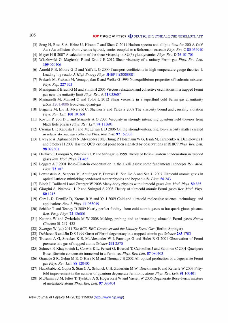
105

[3] Song H, Bass S A, Heinz U, Hirano T and Shen C 2011 Hadron spectra and elliptic flow for 200 A GeVAu + Au collisions from viscous hydrodynamics coupled to a Boltzmann cascade Phys. Rev. C 83 054910

[4] Meyer H B 2007 A calculation of the shear viscosity in SU(3) gluodynamics Phys. Rev. D 76 101701[5] Wlazlowski G, Magierski P and Drut J E 2012 Shear viscosity of a unitary Fermi gas Phys. Rev. Lett.

109 020406[6] Arnold P B, Moore G D and Yaffe L G 2000 Transport coefficients in high temperature gauge theories 1.

Leading log results J. High Energy Phys. JHEP11(2000)001[7] Prakash M, Prakash M, Venugopalan R and Welke G 1993 Nonequilibrium properties of hadronic mixtures

Phys. Rep. 227 321[8] Massignan P, Bruun G M and Smith H 2005 Viscous relaxation and collective oscillations in a trapped Fermi

gas near the unitarity limit Phys. Rev. A 71 033607[9] Mannarelli M, Manuel C and Tolos L 2012 Shear viscosity in a superfluid cold Fermi gas at unitarity

arXiv:1201.4006 [cond-mat.quant-gas][10] Brigante M, Liu H, Myers R C, Shenker S and Yaida S 2008 The viscosity bound and causality violation

Phys. Rev. Lett. 100 191601[11] Kovtun P, Son D T and Starinets A O 2005 Viscosity in strongly interacting quantum field theories from

black hole physics Phys. Rev. Lett. 94 111601[12] Csernai L P, Kapusta J I and McLerran L D 2006 On the strongly-interacting low-viscosity matter created

in relativistic nuclear collisions Phys. Rev. Lett. 97 152303[13] Lacey R A, Ajitanand N N, Alexander J M, Chung P, Holzmann W G, Issah M, Taranenko A, Danielewicz P

and Stocker H 2007 Has the QCD critical point been signaled by observations at RHIC? Phys. Rev. Lett.98 092301

[14] Dalfovo F, Giorgini S, Pitaevskii L P and Stringari S 1999 Theory of Bose–Einstein condensation in trappedgases Rev. Mod. Phys. 71 463

[15] Leggett A J 2001 Bose–Einstein condensation in the alkali gases: some fundamental concepts Rev. Mod.Phys. 73 307

[16] Lewenstein A, Sanpera M, Ahufinger V, Damski B, Sen De A and Sen U 2007 Ultracold atomic gases inoptical lattices: mimicking condensed matter physics and beyond Adv. Phys. 56 243

[17] Bloch I, Dalibard J and Zwerger W 2008 Many-body physics with ultracold gases Rev. Mod. Phys. 80 885[18] Giorgini S, Pitaevskii L P and Stringari S 2008 Theory of ultracold atomic Fermi gases Rev. Mod. Phys.

80 1215[19] Carr L D, Demille D, Krems R V and Ye J 2009 Cold and ultracold molecules: science, technology, and

applications New J. Phys. 11 055049[20] Schafer T and Teaney D 2009 Nearly perfect fluidity: from cold atomic gases to hot quark gluon plasmas

Rep. Prog. Phys. 72 126001[21] Ketterle W and Zwierlein M W 2008 Making, probing and understanding ultracold Fermi gases Nuovo

Cimento 31 247–422[22] Zwerger W (ed) 2011 The BCS–BEC Crossover and the Unitary Fermi Gas (Berlin: Springer)[23] DeMarco B and Jin D S 1999 Onset of Fermi degeneracy in a trapped atomic gas Science 285 1703[24] Truscott A G, Strecker K E, McAlexander W I, Partridge G and Hulet R G 2001 Observation of Fermi

pressure in a gas of trapped atoms Science 291 2570[25] Schreck F, Khaykovich L, Corwin K L, Ferrari G, Bourdel T, Cubizolles J and Salomon C 2001 Quasipure

Bose–Einstein condensate immersed in a Fermi sea Phys. Rev. Lett. 87 080403[26] Granade S R, Gehm M E, O’Hara K M and Thomas J E 2002 All-optical production of a degenerate Fermi

gas Phys. Rev. Lett. 88 120405[27] Hadzibabic Z, Gupta S, Stan C A, Schunck C H, Zwierlein M W, Dieckmann K and Ketterle W 2003 Fifty-

fold improvement in the number of quantum degenerate fermionic atoms Phys. Rev. Lett. 91 160401[28] McNamara J M, Jeltes T, Tychkov A S, Hogervorst W and Vassen W 2006 Degenerate Bose–Fermi mixture

of metastable atoms Phys. Rev. Lett. 97 080404

New Journal of Physics 14 (2012) 115009 (http://www.njp.org/)

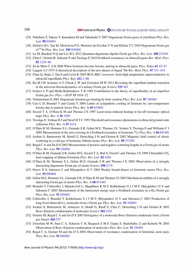
106

[29] Fukuhara T, Takasu Y, Kumakura M and Takahashi Y 2007 Degenerate Fermi gases of ytterbium Phys. Rev.Lett. 98 030401

[30] DeSalvo B J, Yan M, Mickelson P G, Martinez de Escobar Y N and Killian T C 2010 Degenerate Fermi gasof 87Sr Phys. Rev. Lett. 105 030402

[31] Lu M, Burdick N Q and Lev B L 2012 Quantum degenerate dipolar Fermi gas Phys. Rev. Lett. 108 215301[32] Chin C, Grimm R, Julienne P and Tiesinga E 2010 Feshbach resonances in ultracold gases Rev. Mod. Phys.

82 1225–86[33] Sa de Melo C A R 2008 When fermions become bosons: pairing in ultracold gases Phys. Today 61 45–51[34] Leggett A J 1975 A theoretical description of the new phases of liquid 3He Rev. Mod. Phys. 47 331–414[35] Chen Q, Stajic J, Tan S and Levin K 2005 BCS–BEC crossover: from high temperature superconductors to

ultracold superfluids Phys. Rep. 412 1–88[36] Ku M J H, Sommer A T, Cheuk L W and Zwierlein M W 2012 Revealing the superfluid lambda transition

in the universal thermodynamics of a unitary Fermi gas Science 335 563[37] Gorkov L P and Melik-Barkhudarov T K 1962 Contribution to the theory of superfluidity in an imperfect

Fermi gas Sov. Phys.—JETP 13 1018–22[38] Timmermans E 2001 Degenerate fermion gas heating by hole creation Phys. Rev. Lett. 87 240403[39] Carr L D, Bourdel T and Castin Y 2004 Limits of sympathetic cooling of fermions by zero-temperature

bosons due to particle losses Phys. Rev. A 69 033603[40] Savard T A, O’Hara K M and Thomas J E 1997 Laser-noise-induced heating in far-off resonance optical

traps Phys. Rev. A 56 1095[41] Tiesinga E, Verhaar B J and Stoof H T C 1993 Threshold and resonance phenomena in ultracold ground-state

collisions Phys. Rev. A 47 4114[42] O’Hara K M, Hemmer S L, Granade S R, Gehm M E, Thomas J E, Venturi V, Tiesinga E and Williams C J

2002 Measurement of the zero crossing in a Feshbach resonance of fermionic 6Li Phys. Rev. A 66 041401[43] Jochim S, Bartenstein M, Hendl G, Denschlag J H and Grimm R 2002 Magnetic field control of elastic

scattering in a cold gas of fermionic lithium atoms Phys. Rev. Lett. 89 273202[44] Regal C A and Jin D S 2003 Measurement of positive and negative scattering lengths in a Fermi gas of atoms

Phys. Rev. Lett. 90 230404[45] O’Hara K M, Granade S R, Gehm M E, Savard T A, Bali S, Freed C and Thomas J E 1999 Ultrastable CO2

laser trapping of lithium Fermions Phys. Rev. Lett. 82 4204[46] O’Hara K M, Hemmer S L, Gehm M E, Granade S R and Thomas J E 2002 Observation of a strongly

interacting degenerate Fermi gas of atoms Science 298 2179[47] Petrov D S, Salomon C and Shlyapnikov G V 2004 Weakly bound dimers of fermionic atoms Phys. Rev.

Lett. 93 090404[48] Gehm M E, Hemmer S L, Granade S R, O’Hara K M and Thomas J E 2003 Mechanical stability of a strongly

interacting Fermi gas of atoms Phys. Rev. A 68 011401[49] Bourdel T, Cubizolles J, Khaykovich L, Magalhaes K M F, Kokkelmans S J J M F, Shlyapnikov G V and

Salomon C 2003 Measurement of the interaction energy near a Feshbach resonance in a 6Li Fermi gasPhys. Rev. Lett. 91 020402

[50] Cubizolles J, Bourdel T, Kokkelmans S J J M F, Shlyapnikov G V and Salomon C 2003 Production oflong-lived ultracold Li2 molecules from a Fermi gas Phys. Rev. Lett. 91 240401

[51] Jochim S, Bartenstein M, Altmeyer A, Hendl G, Riedl S, Chin C, Denschlag J H and Grimm R 2003Bose–Einstein condensation of molecules Science 302 2101

[52] Greiner M, Regal C A and Jin D S 2003 Emergence of a molecular Bose–Einstein condensate from a Fermigas Nature 426 537

[53] Zwierlein M W, Stan C A, Schunck C H, Raupach S M F, Gupta S, Hadzibabic Z and Ketterle W 2003Observation of Bose–Einstein condensation of molecules Phys. Rev. Lett. 91 250401

[54] Regal C A, Greiner M and Jin D S 2004 Observation of resonance condensation of fermionic atom pairsPhys. Rev. Lett. 92 040403

New Journal of Physics 14 (2012) 115009 (http://www.njp.org/)

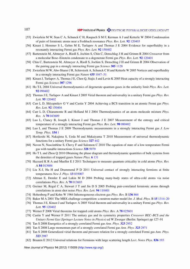
107

[55] Zwierlein M W, Stan C A, Schunck C H, Raupach S M F, Kerman A J and Ketterle W 2004 Condensationof pairs of fermionic atoms near a Feshbach resonance Phys. Rev. Lett. 92 120403

[56] Kinast J, Hemmer S L, Gehm M E, Turlapov A and Thomas J E 2004 Evidence for superfluidity in aresonantly interacting Fermi gas Phys. Rev. Lett. 92 150402

[57] Bartenstein M, Altmeyer A, Riedl S, Jochim S, Chin C, Denschlag J H and Grimm R 2004 Crossover froma molecular Bose–Einstein condensate to a degenerate Fermi gas Phys. Rev. Lett. 92 120401

[58] Chin C, Bartenstein M, Altmeyer A, Riedl S, Jochim S, Denschlag J H and Grimm R 2004 Observation ofthe pairing gap in a strongly interacting Fermi gas Science 305 1128

[59] Zwierlein M W, Abo-Shaeer J R, Schirotzek A, Schunck C H and Ketterle W 2005 Vortices and superfluidityin a strongly interacting Fermi gas Nature 435 1047–51

[60] Kinast J, Turlapov A, Thomas J E, Chen Q, Stajic J and Levin K 2005 Heat capacity of a strongly interactingFermi gas Science 307 1296

[61] Ho T-L 2004 Universal thermodynamics of degenerate quantum gases in the unitarity limit Phys. Rev. Lett.92 090402

[62] Thomas J E, Turlapov A and Kinast J 2005 Virial theorem and universality in a unitary Fermi gas Phys. Rev.Lett. 95 120402

[63] Carr L D, Shlyapnikov G V and Castin Y 2004 Achieving a BCS transition in an atomic Fermi gas Phys.Rev. Lett. 92 150404

[64] Carr L D, Chiaramonte R and Holland M J 2004 Thermodynamics of an atom–molecule mixture Phys.Rev. A 70 043609

[65] Luo L, Clancy B, Joseph J, Kinast J and Thomas J E 2007 Measurement of the entropy and criticaltemperature of a strongly interacting Fermi gas Phys. Rev. Lett. 98 080402

[66] Luo L and Thomas J E 2009 Thermodynamic measurements in a strongly interacting Fermi gas J. LowTemp. Phys. 154 1

[67] Horikoshi M, Nakajima S, Ueda M and Mukaiyama T 2010 Measurement of universal thermodynamicfunctions for a unitary Fermi gas Science 327 442

[68] Navon N, Nascimbene S, Chevy F and Salomon C 2010 The equation of state of a low-temperature Fermigas with tunable interactions Science 328 5979

[69] Ho T L and Zhou Q 2010 Obtaining the phase diagram and thermodynamic quantities of bulk systems fromthe densities of trapped gases Nature Phys. 6 131

[70] Hazzard K R A and Mueller E J 2011 Techniques to measure quantum criticality in cold atoms Phys. Rev.A 84 013604

[71] Liu X-J, Hu H and Drummond P D 2011 Universal contact of strongly interacting fermions at finitetemperatures New J. Phys. 13 035007

[72] Altman E, Demler E and Lukin M D 2004 Probing many-body states of ultra-cold atoms via noisecorrelations Phys. Rev. A 70 013603

[73] Greiner M, Regal C A, Stewart J T and Jin D S 2005 Probing pair-correlated fermionic atoms throughcorrelations in atom shot noise Phys. Rev. Lett. 94 110401

[74] Hohenberg P and Kohn W 1964 Inhomogeneous electron gas Phys. Rev. B 136 864[75] Baker M A 2001 The MBX challenge competition: a neutron matter model Int. J. Mod. Phys. B 15 1314–20[76] Thomas J E, Kinast J and Turlapov A 2005 Virial theorem and universality in a unitary Fermi gas Phys. Rev.

Lett. 95 120402[77] Werner F 2008 Virial theorems for trapped cold atoms Phys. Rev. A 78 025601[78] Castin Y and Werner F 2011 The unitary gas and its symmetry properties Crossover BEC–BCS and the

Unitary Fermi Gas (Springer Lecture Notes in Physics) ed W Zwerger (Berlin: Springer) pp 127–91[79] Tan S 2008 Energetics of a strongly correlated Fermi gas Ann. Phys. 323 2952[80] Tan S 2008 Large momentum part of a strongly correlated Fermi gas Ann. Phys. 323 2971[81] Tan S 2008 Generalized virial theorem and pressure relation for a strongly correlated Fermi gas Ann. Phys.

323 2987[82] Braaten E 2012 Universal relations for Fermions with large scattering length Lect. Notes Phys. 836 193

New Journal of Physics 14 (2012) 115009 (http://www.njp.org/)

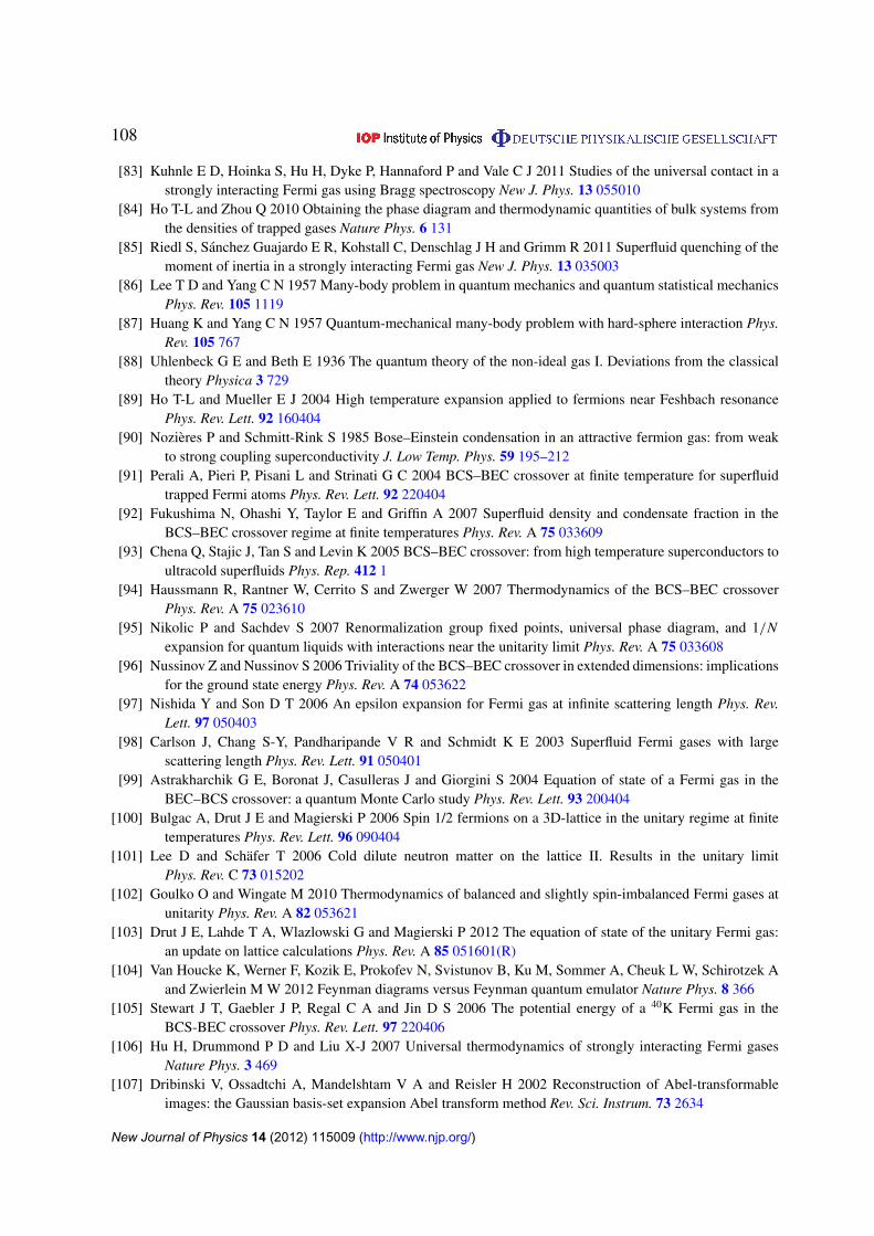
108

[83] Kuhnle E D, Hoinka S, Hu H, Dyke P, Hannaford P and Vale C J 2011 Studies of the universal contact in astrongly interacting Fermi gas using Bragg spectroscopy New J. Phys. 13 055010

[84] Ho T-L and Zhou Q 2010 Obtaining the phase diagram and thermodynamic quantities of bulk systems fromthe densities of trapped gases Nature Phys. 6 131

[85] Riedl S, Sanchez Guajardo E R, Kohstall C, Denschlag J H and Grimm R 2011 Superfluid quenching of themoment of inertia in a strongly interacting Fermi gas New J. Phys. 13 035003

[86] Lee T D and Yang C N 1957 Many-body problem in quantum mechanics and quantum statistical mechanicsPhys. Rev. 105 1119

[87] Huang K and Yang C N 1957 Quantum-mechanical many-body problem with hard-sphere interaction Phys.Rev. 105 767

[88] Uhlenbeck G E and Beth E 1936 The quantum theory of the non-ideal gas I. Deviations from the classicaltheory Physica 3 729

[89] Ho T-L and Mueller E J 2004 High temperature expansion applied to fermions near Feshbach resonancePhys. Rev. Lett. 92 160404

[90] Nozieres P and Schmitt-Rink S 1985 Bose–Einstein condensation in an attractive fermion gas: from weakto strong coupling superconductivity J. Low Temp. Phys. 59 195–212

[91] Perali A, Pieri P, Pisani L and Strinati G C 2004 BCS–BEC crossover at finite temperature for superfluidtrapped Fermi atoms Phys. Rev. Lett. 92 220404

[92] Fukushima N, Ohashi Y, Taylor E and Griffin A 2007 Superfluid density and condensate fraction in theBCS–BEC crossover regime at finite temperatures Phys. Rev. A 75 033609

[93] Chena Q, Stajic J, Tan S and Levin K 2005 BCS–BEC crossover: from high temperature superconductors toultracold superfluids Phys. Rep. 412 1

[94] Haussmann R, Rantner W, Cerrito S and Zwerger W 2007 Thermodynamics of the BCS–BEC crossoverPhys. Rev. A 75 023610

[95] Nikolic P and Sachdev S 2007 Renormalization group fixed points, universal phase diagram, and 1/Nexpansion for quantum liquids with interactions near the unitarity limit Phys. Rev. A 75 033608

[96] Nussinov Z and Nussinov S 2006 Triviality of the BCS–BEC crossover in extended dimensions: implicationsfor the ground state energy Phys. Rev. A 74 053622

[97] Nishida Y and Son D T 2006 An epsilon expansion for Fermi gas at infinite scattering length Phys. Rev.Lett. 97 050403

[98] Carlson J, Chang S-Y, Pandharipande V R and Schmidt K E 2003 Superfluid Fermi gases with largescattering length Phys. Rev. Lett. 91 050401

[99] Astrakharchik G E, Boronat J, Casulleras J and Giorgini S 2004 Equation of state of a Fermi gas in theBEC–BCS crossover: a quantum Monte Carlo study Phys. Rev. Lett. 93 200404

[100] Bulgac A, Drut J E and Magierski P 2006 Spin 1/2 fermions on a 3D-lattice in the unitary regime at finitetemperatures Phys. Rev. Lett. 96 090404

[101] Lee D and Schafer T 2006 Cold dilute neutron matter on the lattice II. Results in the unitary limitPhys. Rev. C 73 015202

[102] Goulko O and Wingate M 2010 Thermodynamics of balanced and slightly spin-imbalanced Fermi gases atunitarity Phys. Rev. A 82 053621

[103] Drut J E, Lahde T A, Wlazlowski G and Magierski P 2012 The equation of state of the unitary Fermi gas:an update on lattice calculations Phys. Rev. A 85 051601(R)

[104] Van Houcke K, Werner F, Kozik E, Prokofev N, Svistunov B, Ku M, Sommer A, Cheuk L W, Schirotzek Aand Zwierlein M W 2012 Feynman diagrams versus Feynman quantum emulator Nature Phys. 8 366

[105] Stewart J T, Gaebler J P, Regal C A and Jin D S 2006 The potential energy of a 40K Fermi gas in theBCS-BEC crossover Phys. Rev. Lett. 97 220406

[106] Hu H, Drummond P D and Liu X-J 2007 Universal thermodynamics of strongly interacting Fermi gasesNature Phys. 3 469

[107] Dribinski V, Ossadtchi A, Mandelshtam V A and Reisler H 2002 Reconstruction of Abel-transformableimages: the Gaussian basis-set expansion Abel transform method Rev. Sci. Instrum. 73 2634

New Journal of Physics 14 (2012) 115009 (http://www.njp.org/)

109

[108] Forbes M M, Gandolfi S and Gezerlis A 2011 Resonantly interacting fermions in a box Phys. Rev. Lett.106 235303

[109] Endres M G, Kaplan D B, Lee J-W and Nicholson A N 2012 Lattice Monte Carlo calculations for unitaryfermions in a finite box arXiv:1203.3169 [hep-lat]

[110] Chien C-C, Guo H, Wulin D and Levin K 2011 Perfect fluids and bad metals: insights from ultracold Fermigases New J. Phys. 13 075011

[111] Kinast J, Turlapov A and Thomas J E 2004 Breakdown of hydrodynamics in the radial breathing mode of astrongly-interacting Fermi gas Phys. Rev. A 70 051401

[112] Bartenstein M, Altmeyer A, Riedl S, Jochim S, Chin C, Denschlag J H and Grimm R 2004 Collectiveexcitations of a degenerate gas at the BEC–BCS crossover Phys. Rev. Lett. 92 203201

[113] Kinast J, Turlapov A and Thomas J E 2005 Damping of a unitary Fermi gas Phys. Rev. Lett. 94 170404[114] Altmeyer A, Riedl S, Kohstall C, Wright M, Geursen R, Bartenstein M, Chin C, Denschlag J H and Grimm

R 2007 Precision measurements of collective oscillations in the BEC–BCS crossover Phys. Rev. Lett.98 040401

[115] Cao C, Elliott E, Joseph J, Wu H, Petricka J, Schafer T and Thomas J E 2011 Universal quantum viscosityin a unitary Fermi gas Science 331 58

[116] Joseph J, Clancy B, Luo L, Kinast J, Turlapov A and Thomas J E 2007 Sound propagation in a Fermi gasnear a Feshbach resonance Phys. Rev. Lett. 98 170401

[117] Clancy B, Luo L and Thomas J E 2007 Observation of nearly perfect irrotational flow in normal andsuperfluid strongly interacting Fermi gases Phys. Rev. Lett. 99 140401

[118] Stringari S 2004 Collective oscillations of a trapped superfluid Fermi gas near a Feshbach resonanceEurophys. Lett. 65 749

[119] Bulgac A and Bertsch G F 2005 Collective oscillations of a trapped Fermi gas near the unitary limit Phys.Rev. Lett. 94 070401

[120] Son D T 2007 Vanishing bulk viscosities and conformal invariance of unitary Fermi gas Phys. Rev. Lett.98 020604

[121] Dusling K and Schafer T 2011 Elliptic flow of the dilute Fermi gas: from kinetics to hydrodynamics Phys.Rev. A 84 013622

[122] Schafer T 2007 The shear viscosity to entropy density ratio of trapped fermions in the unitarity limit Phys.Rev. A 76 063618

[123] Turlapov A, Kinast J, Clancy B, Luo L, Joseph J and Thomas J E 2008 Is a gas of strongly interacting atomicfermions a nearly perfect fluid? J. Low Temp. Phys. 150 567

[124] Bruun G M and Smith H 2005 Viscosity and thermal relaxation for a resonantly interacting Fermi gas Phys.Rev. A 72 043605

[125] Maxwell J C 1866 On the viscosity or internal friction of air and other gases Proc. R. Soc. Lond. XV 14[126] Bruun G M and Smith H 2007 Frequency and damping of the scissors mode of a Fermi gas Phys. Rev. A

76 045602[127] Schafer T and Chafin C 2012 Scaling flows and dissipation in the dilute Fermi gas at unitarity Lect. Notes

Phys. 836 375[128] Chao J, Braby M and Schafer T 2011 Viscosity spectral functions of the dilute Fermi gas in kinetic theory

New J. Phys. 13 035014[129] Enss T, Haussmann R and Zwerger W 2011 Viscosity and scale invariance in the unitary Fermi gas Ann.

Phys. 326 770–96[130] LeClair A 2011 On the viscosity-to-entropy density ratio for unitary Bose and Fermi gases New J. Phys.

13 055015[131] Khalatnikov I M 1965 Introduction to the Theory of Superfluidity (New York: Benjamin)[132] Taylor E, Hu H, Liu X-J, Pitaevskii L P, Griffin A and Stringari S 2009 First and second sound in a strongly

interacting Fermi gas Phys. Rev. A 80 053601[133] Rupak G and Schafer T 2007 Shear viscosity of a superfluid Fermi gas in the unitarity limit Phys. Rev. A

76 053607

New Journal of Physics 14 (2012) 115009 (http://www.njp.org/)

110

[134] Sommer A, Ku M, Roati G and Zwierlein M W 2011 Universal spin transport in a strongly interacting Fermigas Nature 472 201

[135] Ku M, Sommer A and Zwierlein M W 2011 Spin transport in polaronic and superfluid Fermi gases New J.Phys. 13 055009

[136] Duine R A, Polini M, Raoux A, Stoof H T C and Vignale G 2011 Spin drag in ultracold Fermi mixtures withrepulsive interactions New J. Phys. 13 045010

[137] Muller M and Nguyen H C 2011 Collision-dominated spin transport in graphene and Fermi liquids New J.Phys. 13 035009

[138] Bruun G M 2011 Spin diffusion in Ffermi gases New J. Phys. 13 035005[139] Bruun G M and Pethick C J 2011 Spin diffusion in trapped clouds of strongly interacting cold atoms Phys.

Rev. Lett. 107 255302[140] Kohl M, Moritz H, Stoferle T, Gunter K and Esslinger T 2005 Fermionic atoms in a three dimensional

optical lattice: observing Fermi surfaces, dynamics and interactions Phys. Rev. Lett. 94 080403[141] Leggett A J 2006 What do we know about high Tc? Nature Phys. 2 134[142] Eagles D M 1969 Possible pairing without superconductivity at low carrier concentrations in bulk and thin-

film superconducting semiconductors Phys. Rev. 186 456–63[143] Leggett A J 1980 Modern Trends in the theory of Condensed Matter (Berlin: Springer)[144] Peter H 2010 Buchler microscopic derivation of Hubbard parameters for cold atomic gases Phys. Rev. Lett.

104 090402[145] von Stecher J, Gurarie V, Radzihovsky L and Rey A M 2011 Lattice-induced resonances in one-dimensional

bosonic systems Phys. Rev. Lett. 106 235301[146] Hubbard J 1963 Electron correlations in narrow energy bands Proc. R. Soc. Lond. A 276 238[147] Anderson P W 2002 Superconductivity in high Tc cuprates: the cause is no longer a mystery Phys. Scr.

T102 10[148] Timmermans E, Tommasini P, Hussein M and Kerman A 1999 Feshbach resonances in atomic Bose–Einstein

condensates Phys. Rep. 315 199–230[149] Holland M, Kokkelmans S J J M F, Chiofalo M L and Walser R 2001 Resonance superfluidity in a quantum

degenerate Fermi gas Phys. Rev. Lett. 87 120406[150] Kokkelmans S J J M F and Holland M J 2002 Ramsey fringes in a Bose–Einstein condensate between atoms

and molecules Phys. Rev. Lett. 89 180401[151] Milstein J N, Kokkelmans S J J M F and Holland M J 2002 Resonance theory of the crossover from

Bardeen–Cooper–Schrieffer superfluidity to Bose–Einstein condensation in a dilute Fermi gas Phys. Rev.A 66 043604

[152] Ranninger J and Robaszkiewicz S 1985 Superconductivity of locally paired electrons Physica B 135 468[153] Ranninger J and Robin J M 1995 The boson–fermion model of high-Tc superconductivity doping

dependence Physica C 253 279[154] Yang K-Y, Kozik E, Wang X and Troyer M 2011 Diagrammatic quantum Monte Carlo solution of the two-

dimensional cooperon–fermion model Phys. Rev. B 83 214516[155] Carr L D and Holland M J 2005 Quantum phase transitions in the Fermi–Bose Hubbard model Phys. Rev. A

72 031604(R)[156] Zhou F 2005 Mott states under the influence of fermion–boson conversion Phys. Rev. B 72 220501(R)[157] Dickerscheid D B M, van Oosten D, Tillema E J and Stoof H T C 2005 Quantum phases in a resonantly

interacting boson–fermion mixture Phys. Rev. Lett. 94 230404[158] Diener R B and Ho T-L 2006 Fermions in optical lattices swept across Feshbach resonances Phys. Rev. Lett.

96 010402[159] Duan L-M 2005 Effective Hamiltonian for fermions in an optical lattice across a Feshbach resonance Phys.

Rev. Lett. 95 243202[160] Kestner J P and Duan L-M 2010 Effective single-band models for strongly interacting fermions in an optical

lattice Phys. Rev. A 81 043618

New Journal of Physics 14 (2012) 115009 (http://www.njp.org/)

111

[161] Wall M L and Carr L D 2012 Microscopic model for Feshbach interacting fermions in an optical lattice witharbitrary scattering length and resonance width Phys. Rev. Lett. 109 055302

[162] Spuntarelli P P A, Carr L D and Strinati G C 2011 Gray solitons in a strongly interacting superfluid Fermigas New J. Phys. 13 035010

[163] Bolech C J, Baksmaty L O, Lu H and Pu H 2011 A Bogoliubov–de Gennes study of trapped spin-imbalancedunitary Fermi gases New J. Phys. 13 055014

[164] Nowling S, Keranen V, Keski-Vakkuri E and Yogendran K P 2011 Solitons as probes of the structure ofholographic superfluids New J. Phys. 13 065003

[165] Scott R G, Dalfovo F, Pitaevskii L P and Stringari S 2011 Dynamics of dark solitons in a trapped superfluidFermi gas Phys. Rev. Lett. 106 185301

[166] Liao R and Brand J 2011 Traveling dark solitons in superfluid Fermi gases Phys. Rev. A 83 041604[167] Scott R G, Dalfovo F, Pitaevskii L P, Stringari S, Fialko O, Liao R and Brand J 2012 The decay and collisions

of dark solitons in superfluid Fermi gases New J. Phys. 14 023044[168] Nascimbene S, Navon K J, Jiang N, Chevy F and Salomon C 2010 Exploring the thermodynamics of a

universal Fermi gas Nature 463 1057[169] Liao Y-A, Rittner A S C, Paprotta T, Li W, Partridge G B, Hulet R G, Baur S K and Mueller E J 2010

Spin-imbalance in a one-dimensional Fermi gas Nature 467 567[170] Sheehy D E 2011 Spin-selective scatterers as a probe of pairing in a one-dimensional interacting fermion

gas New J. Phys. 13 035015[171] Sadeghzadeh K, Bruun G M, Lobo C, Massignan P and Recati A 2011 Metastability in spin-polarized Fermi

gases and quasiparticle decays New J. Phys. 13 055011[172] Han L and Sa de Melo C A R 2011 Evolution from Bardeen–Cooper–Schrieffer to Bose–Einstein condensate

superfluidity in the presence of disorder New J. Phys. 13 055012[173] Zhang X, Hung C-L, Tung S-K, Gemelke N and Chin C 2011 Exploring quantum criticality based on

ultracold atoms in optical lattices New J. Phys. 13 045011[174] Shlyapnikov G V and Tsvelik A M 2011 Polar phase of one-dimensional bosons with large spin New J.

Phys. 13 065012[175] Braaten E and Hammer H W 2006 Universality in few-body systems with large scattering length Phys. Rep.

428 259–390[176] Wang Y and Esry B D 2011 Universal three-body physics at finite energy near Feshbach resonances New J.

Phys. 13 035025[177] O’Hara K M 2011 Realizing analogues of color superconductivity with ultracold alkali atoms New J. Phys.

13 065011[178] Kinnunen J J, Nummi O H T and Torma P 2011 Coexistence of pairing gaps in three-component Fermi

gases New J. Phys. 13 055013[179] Titvinidze I, Privitera A, Chang S-Y, Diehl S, Baranov M A, Daley A and Hofstetter W 2011 Magnetism

and domain formation in SU(3)-symmetric multi-species Fermi mixtures New J. Phys. 13 035013[180] Alford M G, Schmitt A, Rajagopal K and Schafer T 2008 Color superconductivity in dense quark matter

Rev. Mod. Phys. 80 1455[181] Shuryak E 2009 Physics of strongly coupled quark–gluon plasma Prog. Part. Nucl. Phys. 62 48[182] Heinz U W 2009 Early collective expansion: relativistic hydrodynamics and the transport properties of QCD

matter Relativistic Heavy Ion Physics (Landolt–Boernstein New Series vol 23) ed R Stock (New York:Springer) chapter 5

[183] Braun-Munzinger P and Wambach J 2009 Colloquium: phase diagram of strongly interacting matter Rev.Mod. Phys. 81 1031–50

[184] Casalderrey-Solana J, Liu H, Mateos D, Rajagopal K and Wiedemann U A 2011 Gauge/string duality, hotand heavy QCD ion collisions arXiv:1101.0618 [hep-th]

[185] Arsenne I et al (BRAHMS), Back B et al (PHOBOS), Adcox K et al (PHENIX) and Adams J et al (STAR)2005 First three years of operation of RHIC Nucl. Phys. A 757 1–283

[186] Steinberg P 2012 First results from the LHC heavy ion program New J. Phys. 14 035006

New Journal of Physics 14 (2012) 115009 (http://www.njp.org/)

112

[187] Snellings R 2011 Elliptic flow: brief a review New J. Phys. 13 055008[188] Lisa M A, Frodermann E, Graef G, Mitrovski M, Mount E, Petersen H and Bleicher M 2011 Shape analysis

of strongly interacting systems: the heavy ion case New J. Phys. 13 065006[189] Nagle J L, Bearden I G and Zajc W A 2011 Quark–gluon plasma at RHIC and the LHC: perfect fluid too

perfect? New J. Phys. 13 075004[190] Muller B, Schukraft J and Wyslouch B 2012 First results from Pb + Pb collisions at the LHC Annu. Rev.

Nucl. Part. Sci. 62 361–86 (arXiv:1202.3233 [hep-ex])[191] Coleman S R and Weinberg E J 1973 Radiative corrections as the origin of spontaneous symmetry breaking

Phys. Rev. D 7 1888–910[192] Gross D J and Wilczek F 1973 Ultraviolet behavior of nonabelian gauge theories Phys. Rev. Lett. 30 1343–6[193] Politzer H D 1973 Reliable perturbative results for strong interactions? Phys. Rev. Lett. 30 1346–9[194] Nakamura K et al (Particle Data Group Collaboration) 2010 Review of particle physics J. Phys. G: Nucl.

Part. Phys. 37 075021[195] Gell-Mann M, Oakes R J and Renner B 1968 Behavior of current divergences under SU (3)× SU (3) Phys.

Rev. 175 2195–9[196] Coleman S R and Witten E 1980 Chiral symmetry breakdown in large N chromodynamics Phys. Rev. Lett.

45 100[197] ’t Hooft G 1980 Recent Developments in Gauge Theories (New York: Plenum) p 135

Reprinted in Unity of Forces in the Universe 1982 vol II ed A Zee (Singapore: World Scientific) 1004[198] Asakawa M, Hatsuda T and Nakahara Y 2001 Maximum entropy analysis of the spectral functions in lattice

QCD Prog. Part. Nucl. Phys. 46 459[199] Shuryak E V 1978 Theory of hadronic plasma Sov. Phys.—JETP 47 212–9[200] Shuryak E V 1978 quark–gluon plasma and hadronic production of leptons, photons and psions Phys. Lett.

B 78 150[201] Linde A D 1980 Infrared problem in thermodynamics of the Yang–Mills gas Phys. Lett. B 96 289[202] Pisarski R D and Wilczek F 1984 Remarks on the chiral phase transition in chromodynamics Phys. Rev. D

29 338–41[203] Aoki Y, Endrodi G, Fodor Z, Katz S D and Szabo K K 2006 The order of the quantum chromodynamics

transition predicted by the standard model of particle physics Nature 443 675–8[204] Aoki Y, Fodor Z, Katz S D and Szabo K K 2006 The QCD transition temperature: results with physical

masses in the continuum limit Phys. Lett. B 643 46[205] Aoki Y, Borsanyi S, Durr S, Fodor Z, Katz S D, Krieg S and Szabo K K 2009 The QCD

transition temperature: results with physical masses in the continuum limit II J. High Energy Phys.JHEP06(2009)088

[206] Stephanov M A 2004 QCD phase diagram and the critical point Prog. Theor. Phys. Suppl. 153 139–56[207] Fodor Z and Katz S D 2002 Lattice determination of the critical point of QCD at finite T and mu J. High

Energy Phys. JHEP03(2002)014[208] Allton C R, Ejiri S, Hands S J, Kaczmarek O, Karsch F, Laermann E, Schmidt C and Scorzato L 2002 The

QCD thermal phase transition in the presence of a small chemical potential Phys. Rev. D 66 074507[209] Karsch F, Allton C R, Ejiri S, Hands S J, Kaczmarek O, Laermann E and Schmidt C 2004 Where is the

chiral critical point in three flavor QCD? Nucl. Phys. Proc. Suppl. 129 614–6[210] Fodor S D and Katz Z 2004 Critical point of at QCD finite T and mu, lattice results for physical quark

masses J. High Energy Phys. JHEP04(2004)050[211] de Forcrand P and Philipsen O 2010 Constraining the QCD phase diagram by tricritical lines at imaginary

chemical potential Phys. Rev. Lett. 105 152001[212] Stephanov M A, Rajagopal K and Shuryak E V 1998 Signatures of the tricritical point in QCD Phys. Rev.

Lett. 81 4816–9[213] Gazdzicki M (NA49 and NA61/SHINE Collaborations) 2011 NA49/NA61: results and plans on beam energy

and system size scan at the CERN SPS J. Phys. G: Nucl. Part. Phys. 38 124024

New Journal of Physics 14 (2012) 115009 (http://www.njp.org/)

113

[214] Gupta S, Luo X, Mohanty B, Ritter H G and Xu N 2011 Scale for the phase diagram of quantumchromodynamics Science 332 1525–8

[215] Alford M G, Rajagopal K and Wilczek F 1999 Color flavor locking and chiral symmetry breaking in highdensity QCD Nucl. Phys. B 537 443–58

[216] Schafer T 2000 Patterns of symmetry breaking in at QCD high baryon density Nucl. Phys. B 575 269–84[217] Bedaque P F and Schafer T 2002 High density quark matter under stress Nucl. Phys. A 697 802[218] Schafer T 2006 P-wave meson condensation in high density QCD Phys. Rev. Lett. 96 012305[219] Abuki H, Baym G, Hatsuda T and Yamamoto N 2010 The NJL model of dense three-flavor matter with axial

anomaly: the low temperature critical point and BEC–BCS diquark crossover Phys. Rev. D 81 125010[220] Maeda K, Baym G and Hatsuda T 2009 Simulating dense QCD matter with ultracold atomic boson–fermion

mixtures Phys. Rev. Lett. 103 085301[221] Maeda K 2011 Large expansion N for strongly-coupled Boson Fermion mixtures Ann. Phys. 326 1032–52[222] Rapp A, Zarand G, Honerkamp C and Hofstetter W 2007 Color superfluidity and ‘baryon’ formation in

ultracold fermions Phys. Rev. Lett. 98 160405[223] Shovkovy I A and Wang X 2011 Bulk viscosity in nonlinear and anharmonic regime of strange quark matter

New J. Phys. 13 045018[224] Anglani R, Mannarelli M and Ruggieri M 2011 Collective modes in the color flavor locked phase New J.

Phys. 13 055002[225] Mannarelli M, Colucci G and Manuel C 2011 Dissipative processes in superfluid quark matter AIP Conf.

Proc. 1317 366–71[226] Schafer T 2010 Phase structure and transport properties of dense quark matter arXiv:1001.2917 [astro-

ph.SR][227] Kajantie K, Laine M, Rummukainen K and Schroder Y 2003 The pressure of hot QCD up to g6log(1/g)

Phys. Rev. D 67 105008[228] Kraemmer U and Rebhan A 2004 Advances in perturbative thermal field theory Rep. Prog. Phys. 67 351[229] Blaizot J P, Iancu E and Rebhan A 2003 Thermodynamics of the high-temperature quark gluon plasma

Quark Gluon Plasma vol 3 ed R Hwa and X-N Wang pp 60–122 (arXiv:hep-ph/0303185)[230] D’Hoker E and Freedman D Z 2001 Supersymmetric gauge theories and the AdS/CFT correspondence

Strings 2004 Branes and Extra Dimensions (Proc. TASI 2001) ed S S Gubser and J D Lykken (Singapore:World Scientific) pp 3–160 (arXiv:hep-th/0201253)

[231] Gubser S S, Klebanov I R and Tseytlin A A 1998 Coupling constant dependence in the thermodynamics ofN = 4 supersymmetric Yang–Mills theory Nucl. Phys. B 534 202

[232] Baym G, Monien H, Pethick C J and Ravenhall D G 1990 Transverse interactions and transport in relativisticquark–gluon and electromagnetic plasmas Phys. Rev. Lett. 64 1867

[233] Arnold P, Moore G D and Yaffe L G 2003 Transport coefficients in high temperature gauge theories. II:beyond leading log J. High Energy Phys. JHEP05(2003)051

[234] Danielewicz P and Gyulassy M 1985 Dissipative phenomena in quark gluon plasmas Phys. Rev. D 31 53[235] Policastro G, Son D T and Starinets A O 2001 The shear viscosity of strongly coupled N = 4

supersymmetric Yang–Mills plasma Phys. Rev. Lett. 87 081601[236] Buchel A and Liu J T 2004 Universality of the shear viscosity in supergravity Phys. Rev. Lett. 93 090602[237] Iqbal N and Liu H 2009 Universality of the hydrodynamic limit in AdS/ and the CFT membrane paradigm

Phys. Rev. D 79 025023[238] Gyulassy M and McLerran L 2005 New forms of QCD matter discovered at RHIC Nucl. Phys. A 750 30[239] Teaney D 2006 Finite temperature spectral densities of momentum and R-charge correlators in N = 4 Yang

Mills theory Phys. Rev. D 74 045025[240] Kovtun P and Starinets A 2006 Thermal spectral functions of strongly coupled N = 4 supersymmetric

Yang–Mills theory Phys. Rev. Lett. 96 131601[241] Koch V, Majumder A and Randrup J 2005 Baryon-strangeness correlations: a diagnostic of strongly

interacting matter Phys. Rev. Lett. 95 182301[242] Voloshin S A 2003 Anisotropic flow Nucl. Phys. A 715 379–88

New Journal of Physics 14 (2012) 115009 (http://www.njp.org/)

114

[243] Stock R 2004 Relativistic nucleus–nucleus collisions: from the BEVALAC to RHIC J. Phys. G: Nucl. Part.Phys. 30 S633

[244] Satz H 2008 Maurice Jacob: making quark matter Phys. Scr. 78 028004[245] Baym G 2002 RHIC: from dreams to beams in two decades Nucl. Phys. A 698 XXIII[246] Adams J et al (STAR Collaboration) 2004 Identified particle distributions in pp and Au + Au collisions at

√sN N = 200 GeV Phys. Rev. Lett. 92 112301

[247] Adler S S et al (PHENIX Collaboration) 2004 Identified charged particle spectra and yields in Au + Aucollisions at

√sN N = 200 GeV Phys. Rev. C 69 034909

[248] Miller M L, Reygers K, Sanders S J and Steinberg P 2007 Glauber modeling in high energy nuclear collisionsAnnu. Rev. Nucl. Part. Sci. 57 205–43

[249] Bjorken J D 1983 Highly relativistic nucleus-nucleus collisions: the central rapidity region Phys. Rev. D27 140

[250] Glauber R J 1959 High-Energy Collisions Theory (Lectures in Theoretical Physics vol 1) ed W E Brittin andL G Dunham (New York: Interscience) p 315

[251] Kolb P F, Heinz U W, Huovinen P, Eskola K J and Tuominen K 2001 Centrality dependence of multiplicity,transverse energy, and elliptic flow from hydrodynamics Nucl. Phys. A 696 197

[252] McLerran L D and Venugopalan R 1994 Computing quark and gluon distribution functions for very largenuclei Phys. Rev. D 49 2233

[253] Hirano T, Heinz U W, Kharzeev D, Lacey R and Nara Y 2006 Hadronic dissipative effects on elliptic flowin ultrarelativistic heavy-ion collisions Phys. Lett. B 636 299

[254] Abelev B et al (The ALICE Collaboration) 2010 Charged-particle multiplicity density at mid-rapidity incentral Pb–Pb collisions at

√sN N = 2.76 TeV Phys. Rev. Lett. 105 252301

[255] Fries R J, Kunihiro T, Muller B, Ohnishi A and Schafer A 2009 From 0 to 5000 in 2 · 10−24 seconds: entropyproduction in relativistic heavy-ion collisions Nucl. Phys. A 830 519C–22C

[256] Bazavov A et al 2009 Equation of state and QCD transition at finite temperature Phys. Rev. D 80 014504[257] Bialas A, Bleszynski M and Czyz W 1977 Relation between the Glauber model and classical probability

calculus Acta Phys. Pol. B 8 389–92[258] Bialas A, Bleszynski M and Czyz W 1976 Multiplicity distributions in nucleus–nucleus collisions at high-

energies Nucl. Phys. B 111 461[259] Aamodt K et al (ALICE Collaboration) 2011 Centrality dependence of the charged-particle multiplicity

density at mid-rapidity in Pb–Pb collisions at√

sN N = 2.76 TeV Phys. Rev. Lett. 106 032301[260] Alver B and Roland G 2010 Collision geometry fluctuations and triangular flow in heavy-ion collisions

Phys. Rev. C 81 054905[261] Teaney D and Yan L 2011 Triangularity and dipole asymmetry in heavy ion collisions Phys. Rev. C

83 064904[262] Landau L D 1953 On the multiparticle production in high-energy collisions Izv. Akad. Nauk Ser. Fiz. 17 51[263] Cooper F and Frye G 1974 Comment on the single particle distribution in the hydrodynamic and statistical

thermodynamic models of multiparticle production Phys. Rev. D 10 186[264] Heinz U W 2005 RHIC serves the perfect fluid: hydrodynamic flow of the QGP arXiv:nucl-th/0512051[265] Baym G, Friman B L, Blaizot J P, Soyeur M and Czyz W 1983 Hydrodynamics of ultrarelativistic heavy ion

collisions Nucl. Phys. A 407 541[266] Steinberg P 2005 Landau hydrodynamics and RHIC phenomena Acta Phys. Hung. A 24 51–7[267] Teaney D 2003 Effect of shear viscosity on spectra, elliptic flow, and Hanbury Brown–Twiss radii Phys. Rev.

C 68 034913[268] Adcox K et al (PHENIX Collaboration) 2002 Suppression of hadrons with large transverse momentum in

central Au + Au collisions at√

sN N = 130 GeV Phys. Rev. Lett. 88 022301[269] Ellis S D, Kunszt Z and Soper D E 1990 The one jet inclusive cross-section at order α3

s quarks and gluonsPhys. Rev. Lett. 64 2121

[270] Arleo F 2006 Hard pion and prompt photon at RHIC, from single to double inclusive production J. HighEnergy Phys. JHEP09(2006)015

New Journal of Physics 14 (2012) 115009 (http://www.njp.org/)

115

[271] Aamodt K et al (ALICE Collaboration) 2011 Suppression of charged particle production at large transversemomentum in central Pb–Pb collisions at

√sN N = 2.76 TeV Phys. Lett. B 696 30

[272] Chatrchyan S et al (CMS Collaboration) 2012 Study of high-pT charged particle suppression in PbPbcompared to pp collisions at

√sN N = 2.76 TeV Eur. Phys. J. C 72 1945

[273] Cole B A (ATLAS Collaboration) 2011 Jet probes of√

sN N = 2.76 TeV Pb + Pb collisions with the ATLASdetector J. Phys. G: Nucl. Part. Phys. 38 124021

[274] Baier R, Dokshitzer Y L, Mueller A H, Peigne S and Schiff D 1997 Radiative energy loss of high-energyquarks and gluons in a finite volume quark–gluon plasma Nucl. Phys. B 483 291–320

[275] Salgado C A and Wiedemann U A 2003 Calculating quenching weights Phys. Rev. D 68 014008[276] Adare A et al (PHENIX Collaboration) 2008 Quantitative constraints on the opacity of hot partonic

matter from semi-inclusive single high transverse momentum pion suppression in Au + Au collisions at√

sN N = 200 GeV Phys. Rev. C 77 064907[277] Baier R 2003 Jet quenching Nucl. Phys. A 715 209[278] Bass S A, Gale C, Majumder A, Nonaka C, Qin G-Y, Renk T and Ruppert J 2009 Systematic comparison of

jet energy-loss schemes in a realistic hydrodynamic medium Phys. Rev. C 79 024901[279] Majumder A, Muller B and Wang X-N 2007 Small shear viscosity of a quark–gluon plasma implies strong

jet quenching Phys. Rev. Lett. 99 192301[280] Dusling K, Moore G D and Teaney D 2010 Radiative energy loss and v2 spectra for viscous hydrodynamics

Phys. Rev. C 81 034907[281] Adare A et al (PHENIX Collaboration) 2010 Azimuthal anisotropy of neutral pion production in Au + Au

collisions at√(sN N )= 200 GeV: path-length dependence of jet quenching and the role of initial

geometry Phys. Rev. Lett. 105 142301[282] Adare A et al (PHENIX Collaboration) 2007 Energy loss and flow of heavy quarks in Au + Au collisions at

√sN N = 200 GeV Phys. Rev. Lett. 98 172301

[283] Adler S S et al (PHENIX Collaboration) 2003 Suppressed pi0 production at large transverse momentum incentral Au + Au collisions at

√sN N = 200 GeV Phys. Rev. Lett. 91 072301

[284] Armesto N, Cacciari M, Dainese A, Salgado C A and Wiedemann U A 2006 How sensitive are high-pT

electron spectra at RHIC to heavy quark energy loss? Phys. Lett. B 637 362–6[285] van Hees H, Mannarelli M, Greco V and Rapp R 2008 Nonperturbative heavy-quark diffusion in the

quark–gluon plasma Phys. Rev. Lett. 100 192301[286] Moore G D and Teaney D 2005 How much do heavy quarks thermalize in a heavy ion collision? Phys. Rev.

C 71 064904[287] Adler S S et al (PHENIX Collaboration) 2006 Measurement of identified pi0 and inclusive photon v2

and implication to the direct photon production in√

sN N = 200 GeV Au + Au collisions Phys. Rev. Lett.96 032302

[288] Svetitsky B 1988 Diffusion of charmed quark in the quark gluon plasma Phys. Rev. D 37 2484[289] Herzog C P, Karch A, Kovtun P, Kozcaz C and Yaffe L G 2006 Energy loss of a heavy quark moving through

N = 4 supersymmetric Yang–Mills plasma J. High Energy Phys. JHEP07(2006)013[290] Casalderrey-Solana J and Teaney D 2006 Heavy quark diffusion in strongly coupled N = 4 Yang Mills Phys.

Rev. D 74 085012[291] Gubser S S 2006 Drag force in AdS/CFT Phys. Rev. D 74 126005[292] Gubser S S 2007 Comparing the drag force on heavy quarks in N = 4 super-Yang–Mills theory and QCD

Phys. Rev. D 76 126003[293] Meyer H B 2011 The errant life of a heavy quark in the quark–gluon plasma New J. Phys. 13 035008[294] Riek F and Rapp R 2011 Selfconsistent evaluation of charm and charmonium in the quark–gluon plasma

New J. Phys. 13 045007[295] Israel W 1967 Event horizons in static vacuum space–times Phys. Rev. 164 1776–9[296] Israel W 1968 Event horizons in static electrovac space–times Commun. Math. Phys. 8 245–60[297] Carter B 1971 Axisymmetric black hole has only two degrees of freedom Phys. Rev. Lett. 26 331–3[298] Hawking S W 1971 Gravitational radiation from colliding black holes Phys. Rev. Lett. 26 1344–6

New Journal of Physics 14 (2012) 115009 (http://www.njp.org/)

116

[299] Hawking S W 1972 Black holes in general relativity Commun. Math. Phys. 25 152–66[300] Price R H and Thorne K S 1986 Membrane viewpoint on black holes: properties and evolution of the

stretched horizon Phys. Rev. D 33 915–41[301] Kovtun P, Son D T and Starinets A O 2003 Holography and hydrodynamics: diffusion on stretched horizons

J. High Energy Phys. JHEP10(2003)064[302] Maldacena J M 1999 The large-N limit of superconformal field theories and supergravity Int. J. Theor. Phys.

38 1113–33 (arXiv:hep-th/9711200)Maldacena J M 1998 The large-N limit of superconformal field theories and supergravity Adv. Theor. Math.

Phys. 2 231–52[303] Gubser S S, Klebanov I R and Polyakov A M 1998 Gauge theory correlators from noncritical string theory

Phys. Lett. B 428 105–14 (arXiv:hep-th/9802109)[304] Witten E 1998 Anti-de Sitter space and holography Adv. Theor. Math. Phys. 2 253–91 (arXiv:hep-

th/9802150)[305] Aharony O 2003 The NonAdS/nonCFT correspondence, or three different paths to QCD Progress in

String, Field and Particle Theory (Nato Science Series II: Mathematics, Physics and Chemistry vol 104)ed L Baulieu, E Rabinovici, J Harvey, B Pioline and P Windey (Dordrecht: Kluwer) pp 3–24

[306] Son D T 2008 Toward an AdS/cold atoms correspondence: a geometric realization of the Schrodingersymmetry Phys. Rev. D 78 046003

[307] Balasubramanian K and McGreevy J 2008 Gravity duals for non-relativistic CFTs Phys. Rev. Lett.101 061601

[308] Kachru S, Liu X and Mulligan M 2008 Gravity duals of Lifshitz-like fixed points Phys. Rev. D 78 106005[309] Faulkner T and Polchinski J 2011 Semi-holographic Fermi liquids J. High Energy Phys. JHEP06(2011)012[310] Iqbal N, Liu H and Mezei M 2012 Lectures on holographic non-Fermi liquids and quantum phase transitions

String Theory and its Applications (TASI 2010: From MeV to the Planck Scale) ed M Dine, T Banks andS Sachdev (Singapore: World Scientific) pp 707–815

[311] Nickel D and Son D T 2011 Deconstructing holographic liquids New J. Phys. 13 075010[312] Chesler P M and Yaffe L G 2011 Holography and colliding gravitational shock waves in asymptotically

Ad S5 spacetime Phys. Rev. Lett. 106 021601[313] Hartnoll S A 2009 Lectures on holographic methods for condensed matter physics Class. Quantum Grav.

26 224002[314] Hartnoll S A 2009 Quantum critical dynamics from black holes Understanding Quantum Phase Transitions

ed L Carr (Boca Raton FL: CRC) pp 701–23[315] McGreevy J 2010 Holographic duality with a view toward many-body physics Adv. High Energy Phys.

2010 723105[316] Aharony O, Gubser S S, Maldacena J M, Ooguri H and Oz Y 2000 Large N field theories, string theory and

gravity Phys. Rep. 323 183–386[317] Son D T and Starinets A O 2007 Viscosity, black holes and quantum field theory Annu. Rev. Nucl. Part. Sci.

57 95–118[318] Erdmenger J, Evans N, Kirsch I and Threlfall E 2008 Mesons in gauge/gravity duals—a review

Eur. Phys. J. A 35 81–133[319] Herzog C P 2009 Lectures on holographic superfluidity and superconductivity J. Phys. A: Math. Theor.

42 343001[320] Gubser S S and Karch A 2009 From gauge-string duality to strong interactions: a pedestrian’s guide Annu.

Rev. Nucl. Part. Sci. 59 145–68[321] Lee S-S 2010 TASI lectures on emergence of supersymmetry, gauge theory and string in condensed matter

systems arXiv:1009.5127 [hep-th][322] Hughes S A 2005 Trust but verify: the case for astrophysical black holes eConf C0507252(2005)L006[323] Gallo E and Marolf D 2009 Resource letter BH-2: black holes Am. J. Phys. 77 294–307[324] Kadanoff L P 1966 Scaling laws for Ising models near Tc Physics 2 263–72[325] Wilson K G and Kogut J B 1974 The renormalization group and the epsilon expansion Phys. Rep. 12 75–200

New Journal of Physics 14 (2012) 115009 (http://www.njp.org/)

117

[326] Wilson K G 1975 The renormalization group: critical phenomena and the kondo problem Rev. Mod. Phys.47 773

[327] Weinberg S 1965 Infrared photons and gravitons Phys. Rev. 140 B516–24[328] Weinberg S and Witten E 1980 Limits on massless particles Phys. Lett. B 96 59[329] Jenkins A 2009 Constraints on emergent gravity Int. J. Mod. Phys. D 18 2249–55[330] Bousso R 2002 The holographic principle Rev. Mod. Phys. 74 825–74[331] Hooft G 1993 Dimensional reduction in quantum gravity (essay dedicated to Abdus Salam) arXiv:gr-

qc/9310026[332] Susskind L 1995 The World as a hologram J. Math. Phys. 36 6377–96[333] Heemskerk I, Penedones J, Polchinski J and Sully J 2009 Holography from conformal field theory J. High

Energy Phys. JHEP10(2009)079[334] Fitzpatrick L A and Kaplan J 2011 Analyticity and the holographic S-matrix arXiv:1111.6972 [hep-th][335] Heemskerk I and Polchinski J 2011 Holographic and Wilsonian renormalization groups J. High Energy

Phys. JHEP06(2011)031[336] Adams A, Maloney A, Sinha A and Vazquez S E 2009 1/N effects in non-relativistic gauge–gravity duality

J. High Energy Phys. JHEP03(2009)097[337] Hawking S W and Page D N 1983 Thermodynamics of black holes in anti-de Sitter space Commun. Math.

Phys. 87 577[338] Strominger A and Vafa C 1996 Microscopic origin of the Bekenstein–Hawking entropy Phys. Lett. B

379 99–104[339] Iqbal N and Liu H 2009 Real-time response in AdS/CFT with application to spinors Fortsch. Phys.

57 367–84[340] Sachdev S 2001 Quantum Phase Transitions (Cambridge: Cambridge University Press)[341] Hooft G 1974 A planar diagram theory for strong interactions Nucl. Phys. B 72 461–73[342] Coleman S R 1988 1/N Aspects of Symmetry (Cambridge: Cambridge University Press)[343] Silverstein E 2003 AdS and dS entropy from string junctions: or, the function of junction conjunctions

From Fields to Strings vol 3 ed M Shifman et al (Singapore: World Scientific) pp 1848–63 (arXiv:hep-th/0308175)

[344] Balasubramanian V and Kraus P 1999 A stress tensor for anti-de Sitter gravity Commun. Math. Phys.208 413–28

[345] Bianchi M, Freedman D Z and Skenderis K 2001 How to go with an RG flow J. High Energy Phys.JHEP08(2001)041

[346] Bianchi M, Freedman D Z and Skenderis K 2002 Holographic renormalization Nucl. Phys. B 631 159–94[347] Skenderis K 2002 Lecture notes on holographic renormalization Class. Quantum Grav. 19 5849–76[348] Faulkner T, Liu H and Rangamani M 2011 Integrating out geometry: holographic Wilsonian RG and the

membrane paradigm J. High Energy Phys. JHEP08(2011)051[349] Balasubramanian V, Kraus P, Lawrence A E and Trivedi S P 1999 Holographic probes of anti-de Sitter

space–times Phys. Rev. D 59 104021[350] Klebanov I R and Witten E 1999 AdS/CFT correspondence and symmetry breaking Nucl. Phys. B

556 89–114[351] Papadimitriou I and Skenderis K 2004 Correlation functions in holographic RG flows J. High Energy Phys.

JHEP10(2004)075[352] Son D T and Starinets A O 2002 Minkowski space correlators in AdS/CFT correspondence: recipe and

applications J. High Energy Phys. JHEP09(2002)042[353] Maldacena J M 2003 Eternal black holes in anti-de Sitter J. High Energy Phys. JHEP04(2003)021[354] Herzog C P and Son D T 2003 Schwinger–Keldysh propagators from AdS/CFT correspondence J. High

Energy Phys. JHEP03(2003)046[355] Skenderis K and van Rees B C 2008 Real-time gauge/gravity duality Phys. Rev. Lett. 101 081601[356] Witten E 1998 Anti-de Sitter space, thermal phase transition and confinement in gauge theories Adv. Theor.

Math. Phys. 2 505–32 (arXiv:hep-th/9803131)

New Journal of Physics 14 (2012) 115009 (http://www.njp.org/)

118

[357] Kachru S, Karch A and Yaida S 2010 Holographic lattices, dimers and glasses Phys. Rev. D 81 026007[358] Karch A, Kachru S and Yaida S 2011 Adventures in holographic dimer models New J. Phys. 13 035004[359] Cremonini S 2011 The shear viscosity to entropy ratio: a status report Mod. Phys. Lett. B 25 1867–88[360] Brigante M, Liu H, Myers R C, Shenker S and Yaida S 2008 Viscosity bound violation in higher derivative

gravity Phys. Rev. D 77 126006[361] Kats Y and Petrov P 2009 Effect of curvature squared corrections in AdS on the viscosity of the dual gauge

theory J. High Energy Phys. JHEP01(2009)044[362] Buchel A and Myers R C 2009 Causality of holographic hydrodynamics J. High Energy Phys.

JHEP08(2009)016[363] Hofman D M 2009 Higher derivative gravity, causality and positivity of energy in a UV complete QFT Nucl.

Phys. B 823 174–94[364] de Boer J, Kulaxizi M and Parnachev A 2010 Holographic Lovelock gravities and black holes J. High Energy

Phys. JHEP06(2010)008[365] Camanho X O and Edelstein J D 2010 Causality in AdS/CFT and Lovelock theory J. High Energy Phys.

JHEP06(2010)099[366] Camanho X O, Edelstein J D and Paulos M F 2011 Lovelock theories, holography and the fate of the

viscosity bound J. High Energy Phys. JHEP05(2011)127[367] Casalderrey-Solana J and Salgado C A 2007 Introductory lectures on jet quenching in heavy ion collisions

Acta Phys. Pol. B 38 3731–94[368] D’Eramo F, Liu H and Rajagopal K 2011 Jet quenching parameter via soft collinear effective theory (SCET)

Int. J. Mod. Phys. E 20 1610–5[369] Liu H, Rajagopal K and Wiedemann U A 2006 Calculating the jet quenching parameter from AdS/CFT

Phys. Rev. Lett. 97 182301[370] Liu H, Rajagopal K and Wiedemann U A 2007 Wilson loops in heavy ion collisions and their calculation in

AdS/CFT J. High Energy Phys. JHEP03(2007)066[371] Chesler P M, Jensen K, Karch A and Yaffe L G 2009 Light quark energy loss in strongly-coupled N = 4

supersymmetric Yang–Mills plasma Phys. Rev. D 79 125015[372] Arnold P and Vaman D 2011 Jet quenching in hot strongly coupled gauge theories simplified J. High Energy

Phys. JHEP04(2011)027[373] Hubeny V E 2011 Holographic dual of collimated radiation New J Phys. 13 035006[374] Gubser S S 2008 Breaking an Abelian gauge symmetry near a black hole horizon Phys. Rev. D 78 065034[375] Hartnoll S A, Herzog C P and Horowitz G T 2008 Building a holographic superconductor Phys. Rev. Lett.

101 031601[376] Hartnoll S A, Herzog C P and Horowitz G T 2008 Holographic superconductors J. High Energy Phys.

JHEP12(2008)015[377] Herzog C 2011 Solitons as probes of the structure of holographic superfluids New J. Phys. 13 065003[378] Keranen V, Keski-Vakkuri E, Nowling S and Yogendran K P 2009 Dark solitons in holographic superfluids

Phys. Rev. D 80 121901[379] Keranen V, Keski-Vakkuri E, Nowling S and Yogendran K P 2010 Inhomogeneous structures in holographic

superfluids I. Dark solitons Phys. Rev. D 81 126011[380] Basu P, Nogueira F, Rozali M, Stang J B and Van Raamsdonk M 2011 Towards a holographic model of color

superconductivity New J. Phys. 13 055001[381] Mehen T, Stewart I W and Wise M B 2000 Conformal invariance for nonrelativistic field theory Phys. Lett.

B 474 145–52[382] Son D T and Wingate M 2006 General coordinate invariance and conformal invariance in nonrelativistic

physics: unitary Fermi gas Ann. Phys. 321 197–224[383] Nishida Y and Son D T 2007 Nonrelativistic conformal field theories Phys. Rev. D 76 086004[384] Herzog C P, Rangamani M and Ross S F 2008 Heating up Galilean holography J. High Energy Phys.

JHEP11(2008)080

New Journal of Physics 14 (2012) 115009 (http://www.njp.org/)

119

[385] Maldacena J, Martelli D and Tachikawa Y 2008 Comments on string theory backgrounds with non-relativistic conformal symmetry J. High Energy Phys. JHEP10(2008)072

[386] Adams A, Balasubramanian K and McGreevy J 2008 Hot spacetimes for cold atoms J. High Energy Phys.JHEP11(2008)059

[387] Balasubramanian K and McGreevy J 2009 An analytic Lifshitz black hole Phys. Rev. D 80 104039[388] Adams A and Wang J 2011 Towards a non-relativistic holographic superfluid New J. Phys. 13 115008[389] Hartnoll S A, Polchinski J, Silverstein E and Tong D 2010 Towards strange metallic holography J. High

Energy Phys. JHEP04(2010)120[390] Kovtun P and Nickel D 2009 Black holes and non-relativistic quantum systems Phys. Rev. Lett. 102 011602[391] Barbon J L F and Fuertes C A 2009 Ideal gas matching for thermal Galilean holography Phys. Rev. D

80 026006[392] Balasubramanian K and McGreevy J 2011 The particle number in Galilean holography J. High Energy Phys.

JHEP01(2011)137[393] Holstein T, Norton R E and Pincus P 1973 De Haas–van Alphen effect and the specific heat of an electron

gas Phys. Rev. B 8 2649–56[394] Lee S-S 2009 A non-Fermi liquid from a charged black hole: critical a Fermi ball Phys. Rev. D 79 086006[395] Liu H, McGreevy J and Vegh D 2011 Non-Fermi liquids from holography Phys. Rev. D 83 065029[396] Cubrovic M, Zaanen J and Schalm K 2009 String theory, quantum phase transitions and the emergent Fermi-

liquid Science 325 439–44[397] Faulkner T, Liu H, McGreevy J and Vegh D 2011 Emergent quantum criticality, Fermi surfaces and AdS(2)

Phys. Rev. D 83 125002[398] Hartnoll S A and Tavanfar A 2011 Electron stars for holographic metallic criticality Phys. Rev. D 83 046003[399] Hartnoll S A, Hofman D M and Tavanfar A 2011 Holographically smeared Fermi surface: quantum

oscillations and Luttinger count in electron stars Europhys. Lett. 95 31002[400] Iqbal N, Liu H and Mezei M 2012 Semi-local quantum liquids J. High Energy Phys. JHEP04(2012)086[401] Jensen K 2011 Semi-holographic quantum criticality Phys. Rev. Lett. 107 231601[402] Iqbal N, Liu H and Mezei M 2011 Quantum phase transitions in semi-local quantum liquids arXiv:1108.0425

[hep-th][403] Bayntun A, Burgess C P, Dolan B P and Lee S-S 2011 AdS/QHE: towards a holographic description of

quantum hall experiments New J. Phys. 13 035012[404] Janko B, Maly J and Levin K 1997 Pseudogap effects induced by resonant pair scattering Phys. Rev. B

56 R11407[405] Randeria M 1998 Proc. Int. School of Physics ‘Enrico Fermi’ (Course CXXXVI) ed G Iadonisi, J R Schrieffer

and M L Chiafalo (Amsterdam: IOS Press) p 115[406] Chin C, Bartenstein M, Altmeyer A, Riedl S, Jochim S, Hecker Denschlag J and Grimm R 2004 Observation

of the pairing gap in a strongly interacting Fermi gas Science 305 1128[407] Gaebler J P, Stewart J T, Drake T E, Jin D S, Perali A, Pieri P and Strinati G C 2010 Observation of

pseudogap behaviour in a strongly interacting Fermi gas Nature Phys. 6 569[408] Magierski P, Wlazlowski G and Bulgac A 2011 Onset of a pseudogap regime in ultracold Fermi gases Phys.

Rev. Lett. 107 145304[409] Feld M, Frohlich B, Vogt E, Koschorreck M and Kohl M 2011 Observation of a pairing pseudogap in a

two-dimensional Fermi gas Nature 480 75[410] Schirotzek A, Wu C-H, Sommer A and Zwierlein M W 2009 Observation of Fermi polarons in a tunable

Fermi liquid of ultracold atoms Phys. Rev. Lett. 102 230402[411] Lobo C, Recati A, Giorgini S and Stringari S 2006 Normal state of a polarized Fermi gas at unitarity Phys.

Rev. Lett. 97 200403[412] Koschorreck M, Pertot D, Vogt E, Frohlich B, Feld M and Kohl M 2012 Attractive and repulsive Fermi

polarons in two dimensions Nature 485 619[413] Zhang Y, Ong W, Arakelyan I and Thomas J E 2012 Polarons in the radio-frequency spectrum of a quasi-

two-dimensional Fermi gas Phys. Rev. Lett. 108 235302

New Journal of Physics 14 (2012) 115009 (http://www.njp.org/)

120

[414] Taylor E and Randeria M 2010 Viscosity of strongly interacting quantum fluids: spectral functions and sumrules Phys. Rev. A 81 053610

[415] Enss T 2012 Quantum critical transport in the unitary Fermi gas Phys. Rev. A 86 013616[416] Diehl S, Floerchinger S, Gies H, Pawlowski J M and Wetterich C 2010 Functional renormalization group

approach to the BCS–BEC crossover Ann. Phys. 522 615[417] Braaten E and Hammer H-W 2007 Efimov physics in cold atoms Ann. Phys. 322 120[418] Nishida Y and Tan S 2011 Liberating Efimov physics from three dimensions Few Body Syst. 51 191[419] Salger T, Grassert C, Kling S and Weitz M 2011 Klein-tunneling of a quasi-relativistic Bose–Einstein

condensate in an optical lattice Phys. Rev. Lett. 107 240401[420] Tarruell L, Greif D, Uehlinger T, Jotzu G and Esslinger T 2012 Creating, moving and merging Dirac points

with a Fermi gas in a tunable honeycomb lattice Nature 483 302[421] Pilati S, Giorgini S, Modugno M and Prokof’ev N 2010 Dilute Bose gas with correlated disorder: a path

integral Monte Carlo study New J. Phys. 12 073003[422] Adams A and Yaida S 2011 Disordered holographic systems. I: Functional renormalization arXiv:1102.2892

[hep-th][423] Adams A and Yaida S 2012 Disordered holographic systems II: marginal relevance of imperfection

arXiv:1201.6366 [hep-th][424] Jendrzejewski F, Bernard A, Mueller K, Cheinet P, Josse V, Piraud M, Pezze L, Sanchez-Palencia L, Aspect

A and Bouyer P 2012 Three-dimensional localization of ultracold atoms in an optical disordered potentialNature Phys. 8 398–403

[425] Alver B H, Gombeaud C, Luzum M and Ollitrault J-Y 2010 Triangular flow in hydrodynamics and transporttheory Phys. Rev. C 82 034913

[426] Schenke B, Jeon S and Gale C 2012 Higher flow harmonics from (3 + 1)D event-by-event viscoushydrodynamics Phys. Rev. C 85 024901

[427] Song H and Heinz U W 2009 Extracting the QGP viscosity from RHIC data—a status report from viscoushydrodynamics J. Phys. G: Nucl. Part. Phys. 36 064033

[428] Adare A et al (PHENIX Collaboration) 2010 Enhanced production of direct photons in Au + Au collisionsat√

sN N = 200 GeV and implications for the initial temperature Phys. Rev. Lett. 104 132301[429] Martinez M, Ryblewski R and Strickland M 2012 Boost-invariant (2+1)-dimensional anisotropic

hydrodynamics Phys. Rev. C 85 064913[430] Baier R, Mueller A H, Schiff D and Son D T 2001 ‘Bottom up’ thermalization in heavy ion collisions Phys.

Lett. B 502 51–8[431] Arnold P B, Lenaghan J and Moore G D 2003 QCD plasma instabilities and bottom up thermalization J.

High Energy Phys. JHEP08(2003)002[432] Kurkela A and Moore G D 2011 Thermalization in weakly coupled nonabelian plasmas J. High Energy

Phys. JHEP12(2011)044[433] Mueller A H, Shoshi A I and Wong S M H 2006 A possible modified ‘bottom-up’ thermalization in heavy

ion collisions Phys. Lett. B 632 257–60[434] Dusling K 2011 Role of quantum fluctuations in a system with strong fields New J. Phys. 13 035011[435] Kovchegov Y V 2009 Early time dynamics in heavy ion collisions from and from CGC AdS/CFT Nucl.

Phys. A 830 395C–402C[436] Gubser S S 2010 TASI lectures: collisions in anti-de Sitter space, conformal symmetry and holographic

superconductors arXiv:1012.5312 [hep-th][437] Gubser S S, Pufu S S and Yarom A 2009 Off-center collisions in AdS(5) with applications to multiplicity

estimates in heavy-ion collisions J. High Energy Phys. JHEP11(2009)050[438] Meyer H B 2011 Transport properties of the quark–gluon plasma: lattice a perspective QCD Eur. Phys. J. A

47 86[439] Mohanty B (STAR Collaboration) 2011 STAR experiment results from the beam energy scan program at

RHIC J. Phys. G: Nucl. Part. Phys. 38 124023

New Journal of Physics 14 (2012) 115009 (http://www.njp.org/)

121

[440] Mohanty B 2011 Exploring the quantum chromodynamics landscape with high-energy nuclear collisionsNew J. Phys. 13 065031

[441] Stephanov M A 2009 Non-Gaussian fluctuations near the QCD critical point Phys. Rev. Lett. 102 032301[442] de Forcrand P 2009 Simulating QCD at finite density PoS(LAT2009)010 (arXiv:1005.0539 [hep-lat])[443] Van Hove L 1982 Multiplicity dependence of p(T ) spectrum as a possible signal for a phase transition in

hadronic collisions Phys. Lett. B 118 138[444] Steiner A W, Lattimer J M and Brown E F 2010 The equation of state from observed masses and radii of

neutron stars Astrophys. J. 722 33–54[445] Ozel F, Baym G and Guver T 2010 Astrophysical measurement of the equation of state of neutron star matter

Phys. Rev. D 82 101301[446] Lee S-S 2011 Holographic description of large N gauge theory Nucl. Phys. B 851 143–60[447] Douglas M R, Mazzucato L and Razamat S S 2011 Holographic dual of free field theory Phys. Rev. D

83 071701[448] Ryu S and Takayanagi T 2006 Holographic derivation of entanglement entropy from AdS/CFT Phys. Rev.

Lett. 96 181602[449] Nishioka T, Ryu S and Takayanagi T 2009 Holographic entanglement entropy: an overview J. Phys. A:

Math. Theor. 42 504008[450] Casini H and Huerta M 2012 Infinite divisibility, entanglement entropy and minimal surfaces

arXiv:1203.4007 [hep-th][451] Callan R, He J and Headrick M 2012 Strong subadditivity and the covariant holographic entanglement

entropy formula J. High Energy Phys. JHEP06(2012)081[452] Headrick M and Takayanagi T 2007 A holographic proof of the strong subadditivity of entanglement entropy

Phys. Rev. D 76 106013[453] Hubeny V E, Rangamani M and Takayanagi T 2007 A covariant holographic entanglement entropy proposal

J. High Energy Phys. JHEP07(2007)062[454] Hayden P, Headrick M and Maloney A 2011 Holographic mutual information is monogamous

arXiv:1107.2940 [hep-th][455] Casini H, Huerta M and Myers R C 2011 Towards a derivation of holographic entanglement entropy J. High

Energy Phys. JHEP05(2011)036[456] Albash T and Johnson C V 2011 Evolution of holographic entanglement entropy after thermal and

electromagnetic quenches New J. Phys. 13 045017

New Journal of Physics 14 (2012) 115009 (http://www.njp.org/)