strong-axis flexural buckling of castellated and cellular...
TRANSCRIPT

Laura Kinget
columnsStrong-axis flexural buckling of castellated and cellular
Academic year 2014-2015Faculty of Engineering and ArchitectureChairman: Prof. dr. ir. Luc TaerweDepartment of Structural Engineering
Master of Science in Civil EngineeringMaster's dissertation submitted in order to obtain the academic degree of
Supervisors: Dr. ir. Delphine Sonck, Prof. dr. ir.-arch. Jan Belis

Acknowledgements
First of all, I would like to thank my primary supervisor Delphine Sonck. Ever since the exercise
classes of Structural Analysis I, I was impressed by her ability to explain difficult concepts in a
clear and comprehensive way. It was one of the main reasons I wanted to do my thesis under
her supervision, apart from my interest in the subject. This was brought to live during the
lectures on the subject of built-up compression members of Structural Analysis II, given by
Prof. Caspeele. I also owe her gratitude for the strict deadlines she imposed on me: we met
nearly each week and I had to be able to bring something new to her for each appointment. Thus
I constantly had to keep up with my thesis, which was only a benefit in the end. I would like to
thank Prof. Belis and Prof. Debruyckere. During the interim thesis presentations, Prof. Belis
pointed out that I did not use the correct expressions for parent section nor for the moment
of inertia. He also wrote down every comment made during the presentations, which was a
great help afterwards. Prof. Debruyckere on the other hand forced me to look further than the
theoretical research and to consider what is possible in reality regarding column dimensions.
My gratitude also goes to my parents, grandparents and my sister. They always took time
to listen to me when I had some difficulties, and they spoiled me with my favourite food in the
periods leading up to a thesis deadline. I am also indebted to my friends, who were always there
for me when I had a difficult time. Last of all, but not least of all, I would like to thank my
friend Sebastiaan, simply for always being there for me and lifting my mood, something he is
extremely good at.
iii

iv
De auteur geeft toelating deze masterproef voor consultatie beschikbaar te stellen en delen
van de masterproef te kopieren voor persoonlijk gebruik. Elk ander gebruik valt onder de
beperkingen van het auteursrecht, in het bijzonder met betrekking tot de verplichting de bron
uitdrukkelijk te vermelden bij het aanhalen van de resultaten uit deze masterproef.
The author gives permission to make this master dissertation available for consultation
and to copy parts of this master dissertation for personal use. In the case of any other use,
the limitations of the copyright terms have to be respected, in particular with regard to the
obligation to state expressly the source when quoting results from this master dissertation.
Gent, 22 Mei 2015

Abstract
Strong-axis flexural buckling of castellated and cellularcolumns
Laura Kinget
Supervisors: Dr. ir. Delphine Sonck, Prof. dr. ir.-arch. Jan Belis
Master’s dissertation submitted in order to obtain the academic degree of Master of Science in
Civil Engineering
Department of Structural Engineering
Chairman: Prof. dr. ir. Luc Taerwe
Faculty of Engineering and Architecture
Academic year 2014-2015
In this master’s dissertation the influence of the presence of openings in the web of castellated
and cellular columns is investigated. First, the geometry of those members is further studied,
as well as the limitations of fabrication. An overview of the buckling behaviour of columns in
general is given, whereby attention is paid to the adapted residual stress pattern proposed by
Sonck (2014) for castellated and cellular members. The determination of the critical buckling
load for battened compression members is also looked into, as it is expected that the buckling
behaviour of castellated and cellular columns will be comparable to that of battened compression
members. Additionally, approximate formula are studied that predict the additional deflection
of cellular or castellated beams due to the presence of the openings in the web. In essence,
these formula propose an equivalent bending stiffness, in which the influence of the openings is
incorporated, so that this might be used to determine the critical buckling load of castellated
and cellular members. Eventually, the buckling behaviour of said columns obtained in the finite
element program Abaqus is studied, and compared to analytical expressions to determine the
critical buckling load as well as compared to the buckling curves found in Eurocode 3 (CEN,
2005) to determine the buckling resistance.
v

vi

Extended abstract
In this master’s dissertation the influence of the presence of openings in the web of castellated and
cellular columns on their strong-axis buckling behaviour is investigated. The main advantage
of castellated and cellular members is their increased height compared to the parent section,
leading to a larger strong-axis bending capacity compared to an I-section member of the same
weight. Also, as there are openings in the web, no excess material is present in the member
and service ducts can be guided through these openings. Additionally, the members have a nice
aesthetic, so that they are now also used as columns in building.
First, the geometry of those members is further studied. The geometry of cellular members -
steel I-profiles with circular openings in the web - can be described in function of two independent
factors: one describing the diameter of the opening, one describing the width of the part of the
web in between openings (the web post). The geometry of castellated members - steel I-profiles
with hexagonal openings in the web - is described in function of three independent factors:
one describing the increased height of the member, one describing the angle of the hexagonal
opening and one describing the width of the part of the web in between openings. Additionally,
the limitations imposed by fabrication on these factors are considered.
An overview of the buckling behaviour of columns in general is given, whereby both the
critical buckling load and the buckling resistance are studied. For the critical buckling load,
it is proposed to determine the cross-sectional properties in the middle of an opening, so that
the presence of those openings is taken into account. For the buckling resistance, the geometric
and material imperfections are studied that were taken into account in the determination of the
buckling curves found in Eurocode 3 (CEN, 2005). Additionally, the adapted residual stress
pattern proposed by Sonck (2014) for castellated and cellular members is described and will be
used for the determination of the buckling resistance of those members. The determination of
the critical buckling load for battened compression members about the axis that leads through
the battenings is also looked into, as it is expected that the buckling behaviour of castellated and
cellular columns will be comparable to that of battened compression members. These members
experience a decrease in buckling capacity as there is no continuous shear strength along the
axis through the battenings. This reduction of shear stiffness also occurs for castellated and
cellular columns and will have a significant influence on the critical buckling load.
Additionally, approximate formula are studied that predict the additional deflection of cellu-
lar or castellated beams due to the presence of the openings in the web. In essence, these formula
propose an equivalent bending stiffness, in which the influence of the openings is incorporated.
The idea behind this study is that this equivalent bending stiffness might also be used for the
determination of the critical buckling load of castellated and cellular members. However, two
vii
viii
different approximate formula are proposed for the cellular beams, and first the most appropri-
ate one is determined through a parametric study. This is done for three geometries for both
castellated and cellular beams, so that the applicability of the formula is immediately checked
for a wide range of possible geometries. Based on this study, the most appropriate formula
was selected. However, it was also apparent that the formula do not take the increased shear
deformations of the shorter beams into account, hereby diminishing the belief that the critical
buckling load, determined with the equivalent bending stiffness proposed by those formula, will
accurately predict the critical buckling load of castellated and cellular columns.
A parametric study is executed in the finite element program Abaqus to determine the
critical buckling load through a linear buckling analysis, and the buckling resistance by means of
a geometric and material non-linear analysis with imperfections. For the geometric imperfection
the one prescribed in Eurocode 3 (CEN, 2005) is used, and the proposed adapted residual stress
pattern by Sonck (2014) for cellular and castellated members is adopted. For this study a total
of 270 cellular columns were considered and a total of 810 castellated columns.
The results of the parametric study in the finite element program Abaqus were compared
to the numerically determined strong-axis critical buckling load. From this comparison it could
be concluded that due to the openings in the web, increased shear deformations occur that
cause a significant decrease in the critical strong axis buckling capacity for members with a
slenderness λ equal to 0.5 or 1.0. This decrease is larger for parent sections with stocky flanges
in combination with slender webs as the web will deform more for those members due to its
smaller shear stiffness. Also, geometries that correspond to large openings and small widths
of the web post show a larger decrease of the critical major axis buckling load. The strong-
axis critical buckling load was compared to the critical buckling load for castellated and cellular
members approximated as battened compression members. However, the equations to determine
the critical buckling load of said members are based on a derivation whereby the battenings are
assumed as lines. Because of this, the shear stiffness of wide web posts (the parts of the web
in between the openings) was underestimated, leading to an underestimation of the strong-
axis buckling load. The comparison between the critical buckling load, determined with the
equivalent bending stiffness proposed by the formula for the additional deflection of beams due
to the presence of openings in their web, and the critical buckling load determined with the
finite element program was neither satisfactory, as hereby the increased shear deformations are
not taken into account. Hence further research is advised on a proposal for the determination
of an accurate Ncr for castellated and cellular columns.
As no accurate approximation of the critical buckling load was found, no proposal could be
made with respect to the selection of a buckling curve for castellated and cellular columns to
determine the buckling resistance with. This is because the slenderness λ should be expressed
in function of the critical buckling load to obtain an accurate proposal for a buckling curve.
Nonetheless, the results of the analyses were still studied and they implied that the same buckling
curve could be used as for the plain webbed parent sections for slendernesses exceeding one. Yet,
for the shortest columns, with a slenderness of 0.5, a lower buckling curve should be adopted to
take the increased shear deformations that appear in these columns into account.

Contents
Acknowledgements iii
Abstract v
Extended abstract vii
Acronyms and symbols xiii
1 Introduction 1
1.1 Motivation and background . . . . . . . . . . . . . . . . . . . . . . . . . . . . . . 1
1.2 Thesis objectives - research questions . . . . . . . . . . . . . . . . . . . . . . . . . 2
1.3 Scope of the thesis . . . . . . . . . . . . . . . . . . . . . . . . . . . . . . . . . . . 2
I Literature Study 5
2 Cellular and castellated members 7
2.1 General . . . . . . . . . . . . . . . . . . . . . . . . . . . . . . . . . . . . . . . . . 7
2.2 Area of application . . . . . . . . . . . . . . . . . . . . . . . . . . . . . . . . . . . 8
2.3 Geometry . . . . . . . . . . . . . . . . . . . . . . . . . . . . . . . . . . . . . . . . 8
2.4 Geometric constraints . . . . . . . . . . . . . . . . . . . . . . . . . . . . . . . . . 10
2.4.1 Cellular members . . . . . . . . . . . . . . . . . . . . . . . . . . . . . . . . 10
2.4.2 Castellated members . . . . . . . . . . . . . . . . . . . . . . . . . . . . . . 12
3 Flexural buckling of columns 13
3.1 Cross-sectional properties . . . . . . . . . . . . . . . . . . . . . . . . . . . . . . . 14
3.1.1 2T-approach . . . . . . . . . . . . . . . . . . . . . . . . . . . . . . . . . . 15
3.2 Critical buckling load Ncr . . . . . . . . . . . . . . . . . . . . . . . . . . . . . . . 16
3.3 Buckling resistance: buckling curves . . . . . . . . . . . . . . . . . . . . . . . . . 17
3.3.1 Buckling curves of the ECCS . . . . . . . . . . . . . . . . . . . . . . . . . 17
3.3.2 Determination of the buckling resistance NRd . . . . . . . . . . . . . . . . 18
3.3.3 Imperfections . . . . . . . . . . . . . . . . . . . . . . . . . . . . . . . . . . 21
3.3.4 Experimental determination of the residual stresses . . . . . . . . . . . . . 22
3.4 Built-up compression members . . . . . . . . . . . . . . . . . . . . . . . . . . . . 23
3.5 Major-axis flexural buckling of cellular and castellated columns . . . . . . . . . . 25
ix
x CONTENTS
3.5.1 Identification of the buckling capacity of axially loaded cellular columns
(Sweedan, El-Sawy, & Martini, 2009) . . . . . . . . . . . . . . . . . . . . . 25
4 Additional deflection 29
4.1 Approximate formula . . . . . . . . . . . . . . . . . . . . . . . . . . . . . . . . . . 29
4.2 Parametric study . . . . . . . . . . . . . . . . . . . . . . . . . . . . . . . . . . . . 31
4.2.1 Parent sections . . . . . . . . . . . . . . . . . . . . . . . . . . . . . . . . . 31
4.2.2 Determination of the additional deflection . . . . . . . . . . . . . . . . . . 34
4.2.3 Validation of the model . . . . . . . . . . . . . . . . . . . . . . . . . . . . 36
4.2.4 Results . . . . . . . . . . . . . . . . . . . . . . . . . . . . . . . . . . . . . 41
4.2.5 Conclusions . . . . . . . . . . . . . . . . . . . . . . . . . . . . . . . . . . . 51
4.3 Vassallo (2014) . . . . . . . . . . . . . . . . . . . . . . . . . . . . . . . . . . . . . 55
II Numerical investigation 63
5 The numerical model 65
5.1 Element type and mesh . . . . . . . . . . . . . . . . . . . . . . . . . . . . . . . . 65
5.2 General boundary conditions and load application . . . . . . . . . . . . . . . . . 66
5.3 Additional boundary conditions for strong-axis flexural buckling . . . . . . . . . 67
5.4 Different types of analysis . . . . . . . . . . . . . . . . . . . . . . . . . . . . . . . 69
5.5 Validation of the finite element model . . . . . . . . . . . . . . . . . . . . . . . . 70
6 Strong-axis flexural buckling: parametric study 71
6.1 Studied parameters . . . . . . . . . . . . . . . . . . . . . . . . . . . . . . . . . . . 71
6.1.1 Parent sections . . . . . . . . . . . . . . . . . . . . . . . . . . . . . . . . . 71
6.1.2 Geometry of the openings . . . . . . . . . . . . . . . . . . . . . . . . . . . 72
6.1.3 Length of the member . . . . . . . . . . . . . . . . . . . . . . . . . . . . . 74
6.1.4 Load case and boundary conditions . . . . . . . . . . . . . . . . . . . . . . 75
6.1.5 Determination of the class of the cross-section . . . . . . . . . . . . . . . . 75
6.1.6 Types of analysis . . . . . . . . . . . . . . . . . . . . . . . . . . . . . . . . 76
6.2 Critical buckling load Ncr: results . . . . . . . . . . . . . . . . . . . . . . . . . . 76
6.2.1 Comparison between Ncr,abq and Ncr obtained for a battened compression
column . . . . . . . . . . . . . . . . . . . . . . . . . . . . . . . . . . . . . 79
6.2.2 Comparison between Ncr,abq and Ncr obtained with the proposed Ieq in
section 4 . . . . . . . . . . . . . . . . . . . . . . . . . . . . . . . . . . . . . 79
6.3 Buckling resistance NRd: results . . . . . . . . . . . . . . . . . . . . . . . . . . . 82
III Conclusions 87
7 Conclusions 89

CONTENTS xi
IV Appendices 91
A Numerical study of the deflections 93
A.1 Validation of the model . . . . . . . . . . . . . . . . . . . . . . . . . . . . . . . . 93
A.2 Additional deflection of cellular beams subjected to a point load in the middle . 94
B Geometric constraints 97
B.1 Considered sets of geometries for the cellular and castellated members . . . . . . 97
C Parametric study 99
C.1 Overview of the studied geometries . . . . . . . . . . . . . . . . . . . . . . . . . . 99
C.2 Observed local buckling during the parametric study for Ncr . . . . . . . . . . . 101
C.3 Additional results for Ncr . . . . . . . . . . . . . . . . . . . . . . . . . . . . . . . 101
C.4 Observed local failure during the parametric study for NRd . . . . . . . . . . . . 102
C.5 Additional results for NRd . . . . . . . . . . . . . . . . . . . . . . . . . . . . . . . 104
D Further research towards design rules 113
D.1 Evaluation of the deviation between Ncr,abq and Ncr,2T . . . . . . . . . . . . . . . 113
D.1.1 Influence of the width of the web post . . . . . . . . . . . . . . . . . . . . 113
D.1.2 Influence of Af/Aw (area of the flange divided by the area of the web) . . 117
D.2 Preliminary proposal for a design rule to determine the critical buckling load . . 119
D.3 Conclusions . . . . . . . . . . . . . . . . . . . . . . . . . . . . . . . . . . . . . . . 120

xii CONTENTS

Acronyms and symbols
Acronyms
c1 geometry 1 of the cellular type
ca1 geometry 1 of the castellated type
CS cross-sectional class
CTICM Centre Technique Industriel de la Construction Metallique
EC3 Eurocode 3 (CEN, 2005)
ECCS European Convention for Constructional Steelwork
ENV3 European prestandard of EC3 (CEN, 1992)
FB Flexural Buckling
GMNIA Geometric and Material Non-linear Analysis with Imperfections
LBA Linear Buckling Analysis
LPF Load Proportionality Factor
LTB Lateral Torsional Buckling
xiii

xiv CONTENTS
Symbols
General symbols regarding the geometry of the members
α opening angle of a hexagonal opening
`0 length of the opening
A2T A calculated according to the 2T-approach
Aeff effective cross-sectional area for a class 4 cross-section
aeff effective web opening height for a class 4 cross-section
A cross-sectional area
a height of the opening
b width of the flanges of a I-section
c length of the inclined part of a hexagonal opening
d0 diameter of a circular opening
h0 height of the opening
h height of a plain-webbed member (or parent section)
H height of a castellated or cellular member
Iy,2T Iy calculated according to the 2T-approach
Iz,2T Iz calculated according to the 2T-approach
Iy second moment of area about the y-axis (strong axis)
Iz second moment of area about the z-axis (weak axis)
L length of a member
n number of openings in the member
rb cutting width (taken equal to 8 mm)
r fillet radius
tf thickness of the flange
tw thickness of the web
wend width of the end web post
w width of the web post (distance between openings)
Lcr critical buckling length
Material properties
ν Poisson’s ratio
E modulus of elasticity
fy yield stress
G shear modulus

CONTENTS xv
Symbols regarding the failure load
α imperfection factor for flexural buckling
λ non-dimensional slenderness
χ reduction factor for flexural buckling
∆N deviation factor experimental-numerical results (N)
Ncr,2T critical buckling load based on 2T-approach
Ncr critical buckling load
Npl plastic load
NRd normal buckling resistance
N normal (compressive) load
Symbols regarding built-up compression members
Ach cross-sectional area of the chord
Ich moment of inertia of one chord about its own centroid
h0 distance between the centroids of the chords
a′ distance between the centroids of the battenings
Ib moment of inertia of one battening
Ieff effective second moment of area of the built-up member
n number of planes of battenings
Symbols regarding the additional deformation due to the presence of the open-
ings
δadd additional deflection due to the openings
δb pure bending deflection
Symbols used in Vassallo (2014)
δb,add additional deflection due to bending
δv,add additional deflection due to transfer of shear accros the opening
δbwp,add additional deflection due to web post bending
δadd,tot sum of δb,add, δv,add and δbwp,add
δtot total deflection
δtot,abq total deflection determined in Abaqus
δtot,abq, eq. rect. total deflection determined in Abaqus for a beam
with equivalent rectangular openings

xvi CONTENTS
Chapter 1
Introduction
1.1 Motivation and background
Cellular and castellated members - steel I-profiles with circular or hexagonal openings at regular
intervals - have been used in the industry for over 30 years. However, in Belgium they are not
that extensively used. There is no general design code available, so that a certain hesitation exists
to use these members. Nevertheless, cellular and castellated members offer specific advantages.
Due to the construction process an increase in height is obtained, leading to a larger strong-
axis bending capacity compared to an I-section member of the same weight. Also, as there
are openings in the web, no excess material is present in the member. Through these openings
service ducts are often guided, leading to a decrease in the required floor height. According to
ArcelorMittal (ArcelorMittal, 2008a), it is possible to have 8 storeys in a building with the same
height as a 7 storey-building with traditional floor elements. This is a solid economic advantage,
certainly with the current climate of high land prices. A third advantage is the aesthetics of the
cellular or castellated member: due to the openings the beams appear lighter and let more light
into the structure. Because of this aesthetic feel, cellular and castellated members are now also
used as columns.
However, cellular and castellated members also suffer from some disadvantages. As more
operations are necessary to obtain the final member, production costs are higher than for plain-
webbed members. This additional cost can be balanced however by the more economic material
use. As openings are present in the web, cellular and castellated members have a reduced shear
capacity and a modified failure behaviour, both leading to an adapted and more complex design
procedure.
Cellular and castellated beams and columns are most often created by flame-cutting a hot-
rolled parent section in a certain pattern (Fig. 6.10), after which the two halves are translated
and welded back together. This production process creates a profile with a larger height, leading
to a larger strong-axis bending capacity. However it also creates residual stresses within the
member that influence its structural behaviour. These residual stresses will for example cause
a reduction in the critical buckling load and hence have to be included in the design. The
production process also imposes certain geometrical restrictions to available configurations.
As mentioned before, cellular and castellated members are increasingly used as columns.
As such, they are mostly subjected to compression so that the critical buckling load is often
1

2 CHAPTER 1. INTRODUCTION
the determining design criterion. Sonck (2014) investigated the weak-axis flexural buckling
behaviour of castellated and cellular members. However, as this critical buckling load is often
smaller than the major-axis flexural buckling load, buckling will be prevented along the weak-
axis. Hence, it would be valuable to obtain knowledge of the major-axis buckling behaviour of
cellular and castellated columns.
Figure 1.1: Parent sections are flame-cut and welded back together (extracted from ArcelorMittal
(2008a)).
1.2 Thesis objectives - research questions
In this master thesis the major-axis flexural buckling of cellular and castellated columns will be
investigated numerically. Both material and geometric imperfections will be taken into account,
as these have a significant influence on the buckling resistance of the members. The results will
be used to propose a preliminary design method that fits into the approach of the European steel
standard (CEN (2005)), making use of the existing buckling resistance calculation methods.
The following research questions will be answered in this master thesis:
1. How is the critical major axis buckling load influenced by the presence of the openings in
the web?
2. How is the major axis buckling resistance influenced by the presence of the openings in
the web, taking both geometrical and material imperfections into account?
1.3 Scope of the thesis
As this research links up with the PhD thesis of Sonck (2014), the same limitations to the
investigation are used:
• The members are loaded by a constant compressive force
• The I-section members have regularly placed web openings of circular or hexagonal shape
(cellular and castellated members) and are doubly symmetric.

1.3. SCOPE OF THE THESIS 3
• The castellated and cellular members are made from a hot-rolled I-section by using an
oxycutting and welding procedure.
• The members are simply supported with fork supports at the ends.
In the PhD thesis of Sonck (2014), the weak-axis flexural buckling behaviour of cellular and
castellated columns is investigated, as well as lateral-torsional buckling of cellular and castellated
members. The scope of this thesis is to extend the knowledge obtained in the PhD thesis of
Sonck (2014) with the strong-axis flexural buckling behaviour of cellular and castellated columns
loaded in compression.

4 CHAPTER 1. INTRODUCTION
Part I
Literature Study
5

Chapter 2
Cellular and castellated members
2.1 General
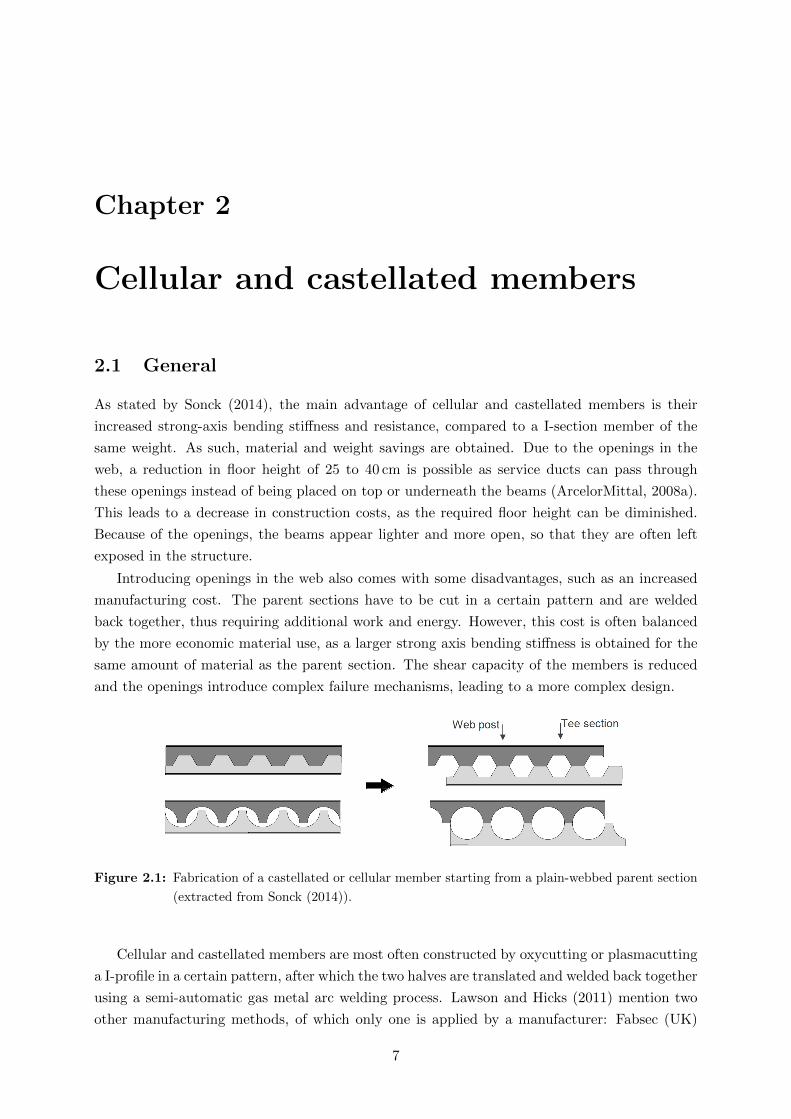
As stated by Sonck (2014), the main advantage of cellular and castellated members is their
increased strong-axis bending stiffness and resistance, compared to a I-section member of the
same weight. As such, material and weight savings are obtained. Due to the openings in the
web, a reduction in floor height of 25 to 40 cm is possible as service ducts can pass through
these openings instead of being placed on top or underneath the beams (ArcelorMittal, 2008a).
This leads to a decrease in construction costs, as the required floor height can be diminished.
Because of the openings, the beams appear lighter and more open, so that they are often left
exposed in the structure.
Introducing openings in the web also comes with some disadvantages, such as an increased
manufacturing cost. The parent sections have to be cut in a certain pattern and are welded
back together, thus requiring additional work and energy. However, this cost is often balanced
by the more economic material use, as a larger strong axis bending stiffness is obtained for the
same amount of material as the parent section. The shear capacity of the members is reduced
and the openings introduce complex failure mechanisms, leading to a more complex design.
Figure 2.1: Fabrication of a castellated or cellular member starting from a plain-webbed parent section
(extracted from Sonck (2014)).
Cellular and castellated members are most often constructed by oxycutting or plasmacutting
a I-profile in a certain pattern, after which the two halves are translated and welded back together
using a semi-automatic gas metal arc welding process. Lawson and Hicks (2011) mention two
other manufacturing methods, of which only one is applied by a manufacturer: Fabsec (UK)
7

8 CHAPTER 2. CELLULAR AND CASTELLATED MEMBERS
welds three plates together to obtain a I-section, after which the openings are cut from the web.
The third mentioned fabrication method is only applied for isolated web openings and involves
the cutting or punching of the opening in the web of a hot-rolled I-section member. All the
other manufacturers (like ArcelorMittal, Westok (UK), Tata Steel (Indian multinational), New
Millenium (USA), Huys-Liggers (The Netherlands) and others) use the first mentioned method.
With this method, also asymmetric sections (composed of two different parent sections), tapered
members and arched or precambered members can be constructed.
2.2 Area of application
Cellular and castellated members are applied in steel and in steel-concrete composite construc-
tion. As their major advantage is the increased strong axis bending stiffness compared to plain-
webbed members of the same weight, they are mostly used as beams in long span applications.
They are commonly subjected to relatively uniform loads because of their limited resistance to
local point loads.
For some applications like roofing, gangways, footbridges or wide-span purlins, low loads
are expected. As the cellular members have to provide sufficient stiffness to the structure, the
height/weight ratio of the members is optimised. This leads to larger openings (h < a < 1.3h)
and smaller openings spacings (0.1a < w < 0.3a). For other applications like floors, carparks,
offshore structures and columns the resistance of the cellular member is of more importance. In
these cases, the load/weight ratio is optimised, leading to smaller openings (0.8h < a < 1.1h)
and larger opening spacings (0.2a < w < 0.7a).(ArcelorMittal, 2008a)
2.3 Geometry
The parent sections are cut according to a certain pattern, translated and welded back together.
The parts of the member above and below the openings are called the tee sections, the part
between two openings is called the web post (Fig. 2.1).
The geometry of the cellular member (Fig. 6.1) is mainly governed by two parameters: the
diameter of the opening a and the width of the web post w. These two parameters determine
the height H of the obtained member (Eq. 2.1) whereas the number of openings n determines
its length L. In Eq. 2.1, rb stands for the cutting width and is taken equal to 8 mm. The
diameter of the opening is most commonly expressed in function of the height h of the original
member, whereas the width of the web post is mostly expressed in function of the diameter of
the opening, as can be seen in Eq. 2.3 and Eq. 2.4.
H = h+
√(a− 2rb)2 − w2
2(2.1)
L = (n− 1) ·w + n · a+ 2 ·wend (2.2)

2.3. GEOMETRY 9
Figure 2.2: Indication of the main parameters of cellular and castellated members (extracted from Sonck
(2014)).
a = fa ·h (2.3)
w = fw · a (2.4)
wend = fwend·w (2.5)
The geometry of the castellated beam can be described in function of three parameters: the
increased height of the member H, the angle of the opening α and the width of the web post w.
The parameters used to describe the geometry can be found in Fig. 6.1. The increased height
of the member can be obtained with Eq. 2.6 and is determined by the factor fH . The angle of
the opening α defines c (Eq. 2.7), together with the length of the hexagonal opening. Because
of the construction process of castellated members the width of the web post is always equal to
the length of the horizontal part of the opening. Hence, the length `0 of the opening is equal to
two times c plus the width of the web post. The width of the web post is defined by the factor
fw as can be seen in Eq. 2.8. The length of the castellated member is found using Eq. 2.9.
H = fHh = h+a
2(2.6)
c =a
2tan(α)(2.7)
w = fw`0 = fw(w + 2c) (2.8)
L = 2 ·wend + n · (w + 2c) + (n− 1) ·w (2.9)
Two different traditional types of castellated geometries are discussed in Grunbauer (2010).
In the first one, the Peiner-Schnittfuhrung, the opening angle α is chosen in such a way that
tan(α)=2. Additionally, H/h is taken equal to 1.5, resulting in an opening height a equal to
h. The width of the web post w is determined as h/2. The Peiner-Schnittfuhrung (PSF) or

10 CHAPTER 2. CELLULAR AND CASTELLATED MEMBERS
Litzka-Schnittfuhrung is most often used in Europe, whereas in Anglo-Saxon countries (UK,
USA and Canada) a similar but slightly different geometry is used. It is characterized by an
opening angle α of 60◦and width of the web post equal to 0.27h.
2.4 Geometric constraints
Several constraints exists for the possible geometries of cellular and castellated beams. These
are imposed due to both practical considerations concerning the production and to ensure the
good mechanical behaviour of the members. As such, they are found in the sales brochure of
ArcelorMittal (2008c), but also in several design guides which are referenced below.
2.4.1 Cellular members
ArcelorMittal (2008a)
H is the total height of the cellular beam and is calculated using formula 2.1.
1.25a ≤ H ≤ 1.75a (2.10)
0.083a ≤ w ≤ 0.8a (2.11)
CTICM (2006)
The following geometric constraints are specified by CTICM (2006). Constraint 2.13 is the same
as 2.11 but results in a stricter upper limit for w. Hence this constraint will be used. Constraint
2.10 is more strict for the dimensions of H than constraint 2.14, so 2.10 will be used. As 2.14
is proposed by the CTICM on behalf of ArcelorMittal, it is introduced to not unnecessarily
complicate the cutting for the manufacturers.
Constraint 1: the ratio between the diameter of the openings and the web thickness must
satisfy:a
tw≤ 90 (2.12)
Constraint 2: the width of the web posts should at least be larger than 50 mm for construction
purposes and must be situated between these values:
0.08a ≤ w < 0.75a (2.13)
In the numerical investigation a width of the web post smaller than 50 mm will be allowed, as
this would exclude a significant number of geometries of the smaller parent sections from the
investigation.
Constraint 3: the ratio of the height of the cellular beam and the diameter of the opening should
satisfy:
1.25a ≤ H ≤ 4a (2.14)

2.4. GEOMETRIC CONSTRAINTS 11
Constraint 4: the web slenderness must satisfy:
hwebtw≤ 124ε with hweb = H − 2tf and ε =
√235
fy(2.15)
Constraint 5: for the cutting operation at least 10 mm should be available between the fillet and
the cut, and the distance between the cut and the flange should be larger than 30 mm (see Fig.
2.3).
hweb,TS − a/2 > 0.01m with hweb,TS =H − 2tf − a
2(2.16)
hweb,TS > 0.03m (2.17)
Figure 2.3: Critical dimensions for cutting (extracted from CTICM (2006)).
ENV3 Annex N (CEN, 1998)
Annex N only applies for geometries that fulfil these conditions. The symbols used for the
constraints are those found in Annex N and are indicated in Fig. 2.4. However, the limits are
very strict and rather outdated compared to the other sources mentioned above. As such, they
are not considered for the determination of the geometries of the numerical investigation.
Figure 2.4: Geometry of beams with multiple openings in the web (extracted from (CEN, 1998)).
12 CHAPTER 2. CELLULAR AND CASTELLATED MEMBERS
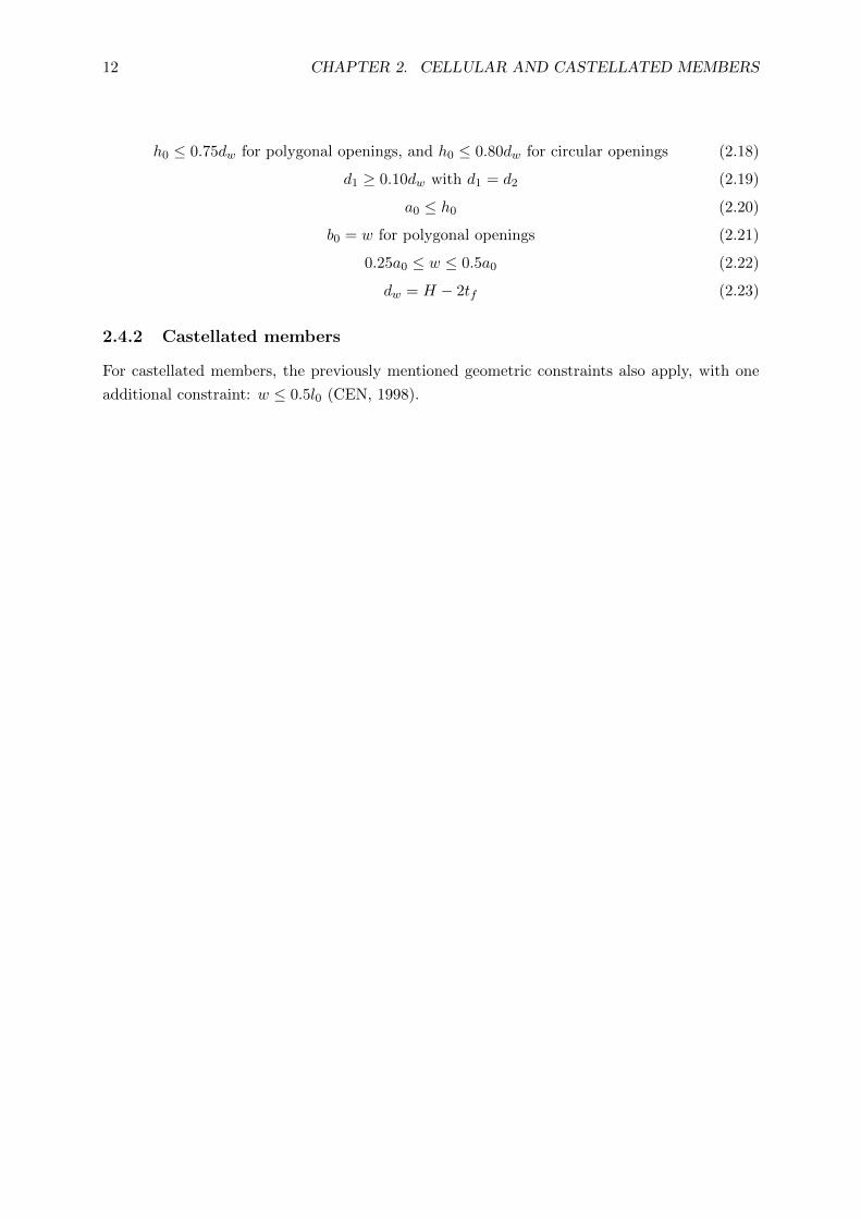
h0 ≤ 0.75dw for polygonal openings, and h0 ≤ 0.80dw for circular openings (2.18)
d1 ≥ 0.10dw with d1 = d2 (2.19)
a0 ≤ h0 (2.20)
b0 = w for polygonal openings (2.21)
0.25a0 ≤ w ≤ 0.5a0 (2.22)
dw = H − 2tf (2.23)
2.4.2 Castellated members
For castellated members, the previously mentioned geometric constraints also apply, with one
additional constraint: w ≤ 0.5l0 (CEN, 1998).

Chapter 3
Flexural buckling of columns
Columns are almost exclusively subjected to compressive axial forces. As such, for slender
members, the buckling behaviour will often be the critical design factor. As castellated members
have been in use since the fifties and cellular members since the eighties, several design guidelines
exist for those members that are applied as beams. However, no guidelines can be found for
the global buckling behaviour of cellular or castellated columns. Sonck (2014) investigated the
lateral-torsional and weak-axis flexural buckling behaviour of cellular and castellated members.
In this master thesis, the strong-axis flexural buckling behaviour will be investigated. As it is a
continuation of the research performed by Sonck (2014), the same constraints are taken for the
research:
• the members are simply supported;
• the members have a doubly symmetric I-section: the centre of gravity G coincides with
the shear centre D and the principal axes coincide with the axes of symmetry;
• the member is loaded by a central axial normal force N;
• the member can develop its full plastic resistance before buckling locally: the member’s
cross-section class is 1 or 2.
The elastic buckling theory (Trahair, 1993) describes how a perfectly straight elastic member
that is loaded in bending or compression can fail suddenly by branching of the load-deflection
path or bifurcation. This sudden failure occurs at the critical load or elastic buckling load. Upon
a further increase in load, small disturbances can cause the member to snap from the original
path (1) to the lower horizontal load path (2) in Fig. 3.1. However, real members are neither
perfectly straight nor exhibit perfect elastic behaviour. Apart from being not perfectly straight,
the member will have certain geometric imperfections and load eccentricities should also be taken
into account. As such, the behaviour will be geometrically non-linear and the load-deflection
path will approach path (3). The material behaviour of steel will rather be elasto-plastic than
elastic, and the material can show imperfections such as residual stresses. Hence, path (4)
represents all imperfections and describes best the real load-deflection behaviour at buckling: a
maximum load is reached that is called the buckling resistance.
13

14 CHAPTER 3. FLEXURAL BUCKLING OF COLUMNS
Figure 3.1: General structural behaviour of a member. Based on (Trahair, 1993)
3.1 Cross-sectional properties
Figure 3.2: Indication of the axes and the dimensions of the member.
As can be seen in Fig. 3.2 the y- and z-axis are the principal axes, the x-axis is along the
length L of the member. The dimensions are also indicated in Fig. 3.2. For the calculation of
the cross-sectional properties a wire model is used, in which it is assumed that the weight of
each part of the cross-section is concentrated at its centreline. This means that the fillets are not
taken into account, but this is partially counteracted by the overlap between the flanges and the
web. However, the thus calculated properties will differ from those present in reality, especially
the torsional constant and the plastic section modulus. As the cross-sectional properties are
determined with the wire model, the wire model approach is also used in the finite element
model to obtain good conformity. The model is composed of shell elements, hence the fillet is
not taken into account. This is not a problem as for the determination of the buckling curves the
dimensionless parameters λ and χ are used. In this format, there is little difference between the
buckling curves obtained with a numerical model with fillets and without fillets (Taras, 2010).
The second moments of area about the y- and z-axis are calculated with Eq. 3.1 and Eq.

3.1. CROSS-SECTIONAL PROPERTIES 15
3.2, and the polar moment of inertia I0 with Eq. 3.3. As can be seen in Fig. 3.2, the y-axis is
the strong axis and the z-axis the weak axis. The area of the cross-section A is calculated with
Eq. 3.4. The torsional constant is given by Eq. 3.1 and the warping constant is given by Eq.
3.6.
Iy = 2bt3f12
+ 2btf
(h− tf
2
)2
+(h− tf )3tw
12(3.1)
Iz = 2b3tf12
+(h− tf )t3w
12(3.2)
I0 = Iy + Iz (3.3)
A = 2btf + (h− tf )tw (3.4)
It =(h− tf )t3w
16
[16
3− 3.36
tw(h− tf )
(1− t4w
12 · (h− tf )4
)]+ (3.5)
2bt3f16
[16
3− 3.36
tfb
(1−
t4f12b4
)]
Iw =h2
2
b3tf12
(3.6)
3.1.1 2T-approach
The 2T-approach is found in CEN (1998) and is a design approach for the calculation of the
lateral-torsional buckling resistance of castellated or cellular members. The design approach is
essentially the same as for plain-webbed I-section members, with the difference that the cross-
sectional properties are calculated in the middle of an opening. It was first proposed by Nethercot
and Kerdal (1982) and Gietzelt and Nethercot (1983), based on full-scale LTB experiments. The
approach is named after the two tees of which the section at the openings consists.
Although this is a design approach for the determination of lateral-torsional buckling resis-
tance, the calculation of the cross-sectional properties at the middle of an opening is withheld.
This way, the presence of the openings is already taken into account in the cross-sectional prop-
erties (Eq. 3.7 till Eq. 3.10), although additional factors might have to be included to be able
to determine the critical buckling load and resistance.
Iy,2T = 2bt3f12
+ 2btf
(H − tf
2
)2
+(H − tf )3tw
12− a3tw
12(3.7)
Iz,2T = 2b3tf12
+(H − tf − a)t3w
12(3.8)
A2T = 2btf + (H − tf − a)tw (3.9)
It,2T =(H − tf − a)t3w
16
[16
3− 3.36
tw(H − tf − a)
(1− t4w
12 · (H − tf − a)4
)]+
2bt3f16
[16
3− 3.36
tfb
(1−
t4f12b4
)](3.10)

16 CHAPTER 3. FLEXURAL BUCKLING OF COLUMNS
3.2 Critical buckling load Ncr
For a doubly symmetric column subjected to a central normal load there are three failure pos-
sibilities: flexural buckling about the weak axis, flexural buckling about the strong axis and
torsional buckling. The critical buckling load Ncr is hence the smallest of the corresponding
normal loads: Ncr,z, Ncr,y and Ncr,t (Eqs. 3.12-3.14)
Ncr = min(Ncr,y, Ncr,z, Ncr,t) (3.11)
Ncr,z =π2EIzL2cr
(3.12)
Ncr,y =π2EIyL2cr
(3.13)
Ncr,t =A
I0
(GIt +
π2EIwL2cr
)(3.14)
Since Iz < Iy (when the boundary conditions are equal), flexural buckling will occur about
the weak axis. Yet, in reality buckling about the weak axis is mostly obstructed to obtain a higher
design load, hence buckling about the strong-axis becomes the governing design criterion. Thus,
this thesis investigates the strong-axis flexural buckling which implies that several boundary
conditions will have to be added to the model to prevent weak-axis buckling. These boundary
conditions will be discussed in part 5.3.
A column can be supported in several ways: pinned, fixed, simply supported with fork
supports, etc. Depending on the support (the boundary condition), different buckling modes
will occur, as is illustrated in Fig. 3.3. This is taken into account in the critical buckling load
Ncr by means of the buckling length Lcr. It equals the actual length L of the column, multiplied
with a factor to account for the different boundary conditions. This factor can be found in part
1-1 of Eurocode 3 (CEN, 2005) for columns part of a frame, or in the national annex of part
1-1 of Eurocode 3 (CEN, 2010). In this thesis, Lcr is equal to L as the columns are simply
supported.
Figure 3.3: Different buckling modes (extracted from Van Impe (2011)).

3.3. BUCKLING RESISTANCE: BUCKLING CURVES 17
3.3 Buckling resistance: buckling curves
The expressions in the previous part give the critical buckling load for perfectly straight, elastic
members. However, a real member is neither perfectly straight, nor will it exhibit perfect elastic
behaviour. This is taken into account in the buckling resistance of a member, which is, according
to Eurocode 3 (CEN, 2005), determined by:
• the elastic critical buckling load, that incorporates the effects of the member’s geometry
and elastic stiffness and the boundary conditions;
• the plastic resistance, governed by the member’s yield stress and geometry;
• the imperfections, either geometric imperfections (e.g. eccentric load application, not
perfectly straight member) or material imperfections (e.g.. residual stresses) or both.
These determine the applicable buckling curve.
The buckling curves were proposed by the ECCS (1978) and will be discussed in part 3.3.1.
Based on these buckling curves, the buckling resistance NRd is determined.
3.3.1 Buckling curves of the ECCS
The ECCS, the European Convention for Constructional Steelwork, introduced five buckling
curves in 1978 to determine the actual strength of columns. These are the same buckling curves
that appear in the current European Standard EN 1993 1-1 (CEN, 2005). The buckling curves
were the result of extensive experiments on more than 1000 profiles with different cross-sections,
different values of slenderness, different fabrication processes and different types of steel. After
fabrication, no straightening process was executed on the member, as this might be beneficial for
the residual stress pattern. The experiments were combined with numerous GMNIA analyses
(geometrically and materially non-linear analysis with imperfections included) that took both
residual stresses and a geometric imperfection into account. For the geometric imperfection a
lateral half sine was assumed with an amplitude of L/1000. It was assumed that the effect of
load eccentricities was also covered with this amplitude. The residual stress pattern taken into
account is displayed in Fig. 3.5. Compared with the influence of this stress pattern the variation
of yield stress across the section could be neglected. There was a good agreement between the
numerical results found with these imperfections and the mean values minus twice the standard
deviation (m-2s) of the test results (Van Impe, 2011).
The selection of a buckling curve is based on the shape of the cross section of the profile,
the axis about which buckling occurs and on the fabrication process (hot-rolled or welded). For
different shapes of cross sections, the choice of the buckling curve is summarized in tables, of
which a short example is given in table 3.1. As can be seen in this table, the depth to width
ratio and the thickness of the flanges have a significant influence on the choice of the buckling
curve. As the depth to width ratio (h/b ≤ 1.2) decreases, the buckling curve lies lower. The
thicker the flange, the lower the buckling curve lies. For flanges thicker than 40 mm the residual
stresses vary across the width of the flange to the extent where the stresses due to hot-rolling
or welding can reach fy at the edge of the flange. The residual stresses have so much influence
that they necessitated the existence of the fifth buckling curve, curve d (Van Impe, 2011).

18 CHAPTER 3. FLEXURAL BUCKLING OF COLUMNS
0.0 0.5 1.0 1.5 2.0 2.5 3.0
λ [-]
0.0
0.2
0.4
0.6
0.8
1.0
1.2
χ[-
]χel
a0
a
b
c
d
Flexural buckling curves
Figure 3.4: Eurocode 3 buckling curves (CEN, 2005).
It can also be noted from this table that the buckling curve for buckling about the z-axis lies
lower than the curve for buckling around the y-axis. The bending stiffness about the z-axis at
the moment of yielding is decreased due to the compressive residual stresses in the tips of the
flanges. For buckling about the y-axis, the effect of these residual stresses is partly compensated
by the residual stresses in the middle of the flanges (Van Impe, 2011).
3.3.2 Determination of the buckling resistance NRd
The buckling resistance of a column is determined by means of Eq. 3.15. In this, χ stands for
the reduction factor that is described by the buckling curves and can be found with equation
3.16. The reduction factor is mainly determined by the equivalent slenderness λ (Eq. 3.17) and
the imperfection parameter α. For small values of λ, the reduction factor approaches χpl = 1
so that the plastic resistance is dominant. For large values of λ the reduction factor approaches
χel = 1/λ2 so that the critical buckling load Ncr determines NRd. For intermediate values of λ
(between 0.5 and 1.5) the imperfections have the most influence.
The imperfection parameter α corresponds with a specific buckling curve and is as such
dependent on the geometry of the cross-section, the buckling direction and the yield stress fy.
The to be used buckling curve is determined based on limits as those found in table 3.1, and
the imperfection parameter is then found in Table 3.2.
Nb,Rd =χAfyγM1
(3.15)
χ =1
φ+(φ2 − λ2
)0.5 with φ = 0.5(1 + α
(λ− 0.2
)+ λ2
)(3.16)

3.3. BUCKLING RESISTANCE: BUCKLING CURVES 19
Table 3.1: Table to determine the buckling curve (extracted from CEN (2005)).
Type Limits Buckling axis Buckling curve
S460
Rolled I-sections h/b>1.2 y-y a a0
tf ≤ 40 mm z-z b a0
40 mm < tf ≤100 mm y-y b a
z-z c a
h/b≤1.2 y-y b a
tf ≤100 mm z-z c a
tf >100 mm y-y d c
z-z d c
Welded I-sections tf ≤ 40 mm y-y b b
z-z c c
tf > 40 mm y-y c c
z-z d d
Table 3.2: Imperfection parameter α.
Buckling curve a0 a b c d
α 0.13 0.21 0.34 0.49 0.76
λ =
√AfyNcr
(3.17)
Ncr =π2EI
L2cr
(3.18)
To determine the properties of the cross section, the classification of the cross section must
be known first. This is discussed below in paragraph 3.3.2. These properties are used to
calculate the critical buckling load Ncr and the equivalent slenderness λ (Eq. 3.18 and Eq.
3.17). Subsequently, the to be used buckling curve is determined based on limits as those found
in table 3.1. With a certain buckling curve corresponds an imperfection parameter α that is
found in table 3.2. The imperfection parameter and the equivalent slenderness are used to
determine the reduction coefficient χ (Eq. 3.16), which is needed to find the buckling resistance
Nb,Rd (Eq. 3.15). In this equation γM1 is taken equal to 1 for buildings, as prescribed in the
EC3 (CEN, 2005).
Classification of the cross-section (CEN, 2005)
Cross-sections are divided into four classes to indicate their limitation of resistance and rotational
capacity due to the local buckling resistance. Cross-sections of class 1 and 2 can develop their full
plastic moment resistance, however the rotation capacity for cross-sections of class 2 is limited
due to local buckling. Cross-sections of class 3 will not develop their plastic resistance as local

20 CHAPTER 3. FLEXURAL BUCKLING OF COLUMNS
buckling will occur sooner. Yet, they can reach the yield strength in the extreme compression
fibre of the member, assuming an elastic distribution of stresses. For cross-sections of class 4,
local buckling will occur before the yield strength is reached in any part of the cross-section.
In case the cross-section belongs to class 4, the slenderness λ and the buckling resistance
Nb,Rd should be determined based on an effective cross-section as indicated in Eq. 3.19 and Eq.
3.20. The determination of the effective surface Aeff of the cross section is detailed in section
4.4 of part 1-5 of Eurocode 3 (CEN, 2006). It implies the introduction of an opening in the
cross-section.
Nb,Rd =χAefffyγM1
(3.19)
λ =
√AefffyNcr
(3.20)
In case of I-profiles subjected to compression, the classification of the cross-section is the
most detrimental of the classification of the web and the classification of the flanges. However,
as there are openings present along the length of the member, the classification of the web must
be determined for the web at the web post (the part between the openings, see Fig. 2.1) as well
as for the web at the center of the opening (the tee section). To determine the classification
of the flanges and of the web at the web post, Table 5.2 of section 5.5 of Eurocode 3 applies
(CEN, 2005). The classification of the web at the tee section can be determined with Annex N
of ENV3 (the European prestandard of Eurocode 3 (CEN, 1998)), in which the local buckling
of the outstanding part of the web at the tee is checked (Sonck, 2014).
The rules from Annex N are given below.

3.3. BUCKLING RESISTANCE: BUCKLING CURVES 21
3.3.3 Imperfections
Material imperfections are those imperfections that are present in the material such as residual
stresses. These are the internal stresses that are present in the member when it is not subjected
to a load. Residual stresses are introduced either by a thermal process, where differential
plastic deformations arise due to uneven cooling, or by a mechanical process like cold-drawing.
Hence, the cutting and welding operation necessary to construct cellular and castellated members
introduces residual stresses into the members. They reduce the buckling strength of a member
as they facilitate the onset of inelastic behaviour. They occur on top of the residual stresses
that were already present in the parent sections due to hot-rolling.
In the fifties, the residual stress pattern in hot-rolled I-section members was studied on
demand of the Column Research Council. The results of this research, done by Beedle, Hubert
and Tall, are summarized in Sonck (2014). A parabolic stress pattern was found along the
flange, with tensile stresses at the centre and compressive stresses at the edges of the flange. As
long as the flange thickness remains small, little variation of this stress pattern was found in the
thickness direction. On the other hand, the sign of the residual stresses in the web depended
on the cross-sectional dimensions. Little variation was found over the length of a member.
Additionally the residual stresses due to cold-straightening were studied. These appeared to be
more random but lower than the thermal residual stresses. As they are more difficult to predict
and as they vary greatly (sometimes they are not present at all, sometimes they have a large
effect), the Manual on Stability of steel Structures from the ECCS (European Convention for
Constructional Steelwork) takes only the thermal residual stresses into account, thus neglecting
the advantageous effect of the straightening operations (ECCS, 1976). The proposed linear
residual stress patterns by the ECCS can be found in Fig. 3.5. This stress pattern is nowadays
considered as the valid residual stress pattern for numerical simulations. (Sonck, 2014)
Figure 3.5: Residual stress distribution for hot-rolled members proposed by the ECCS (extracted from
Sonck (2014))
The operations of cutting and welding necessary to construct a cellular or castellated beam
will alter this stress pattern. Due to cutting, a narrow strip will have tensile stresses equal to
the yield stress fy, and the residual stresses in the remaining part of the plate preserve the
static equilibrium. The same is found at the location of a weld: high tensile stresses at the weld,

22 CHAPTER 3. FLEXURAL BUCKLING OF COLUMNS
balanced by compressive stresses elsewhere in the section.
3.3.4 Experimental determination of the residual stresses
In Sonck (2014) the adaptation of the residual stress pattern due to the presence of the openings
is experimentally determined: starting from six IPE160 parent sections four castellated beams
are fabricated, and two cellular beams. For the cellular beams a special production method is
used: the beam is fabricated like a castellated beam, after which circular openings are cut around
the hexagonal openings. However, this is an additional operation that takes a lot of time as the
oxycutting flame has to be restarted for each opening. Hence, it is a fabrication method that is
not applied in the industry. The results of those two beams are thus theoretically valuable, but
aren’t used to propose an adapted residual stress pattern. Sonck (2014) states that the same
residual stress pattern is expected for the cellular beams fabricated in the general way as for the
castellated beams.
The beams were cold-straightened, but the influence of this operation was negligible on the
measured residual stresses. These were measured in the parent sections, after cutting and after
welding of the members. The residual stress pattern found in the parent sections lies between
the pattern proposed by Young and the pattern proposed by the ECCS (1978) (Fig. 3.5). The
cutting operation had limited influence on this residual stress pattern in the flanges, but in
the web high tensile stresses were found near the cut. After the welding operation these high
tensile stresses were still observed in the web, and high compressive stresses were measured in
the flanges. Hence, from the experimental results it could be concluded that the compressive
residual stresses in the flanges increase due to the production process.
Based on an analytical approximation of the test results, analytical results for the IPE160
sections were compared with analytical results for heavier sections (IPE300, IPE600, HE320A,
HE650A, HE320M and HE650M). From this comparison it was concluded that the same order
of magnitude in σres variations is found in the flanges of both the test specimens and the heavier
sections. Hence, the measurements of the test specimens can be used to estimate the residual
stresses in the heavier sections.
The residual stresses that are present in the flanges influence the global buckling resistance
the most. Hence, the proposed pattern by Sonck (2014) matches the obtained residual stress
variations in the flanges. The resultant of those stresses is a compressive force, that must be
balanced by tensile stresses in the web to obtain no resulting normal force. Hence, a residual
stress decrease of 30 MPa is proposed at the flange tips and a decrease of 20 MPa at the flange
centres compared with the residual stress pattern proposed by the ECCS (1978). To not fur-
ther complicate the pattern along the length of the member, it was chosen to introduce the
tensile equilibrating stresses only in the part of the web that is present along the full length
of the member, thus in the area of the web at the tee sections. This can be done as a study
demonstrated that the area of the web on which the equilibrating stresses were applied is of
no major importance, as long as the yield stress is not reached. The magnitude of the tensile
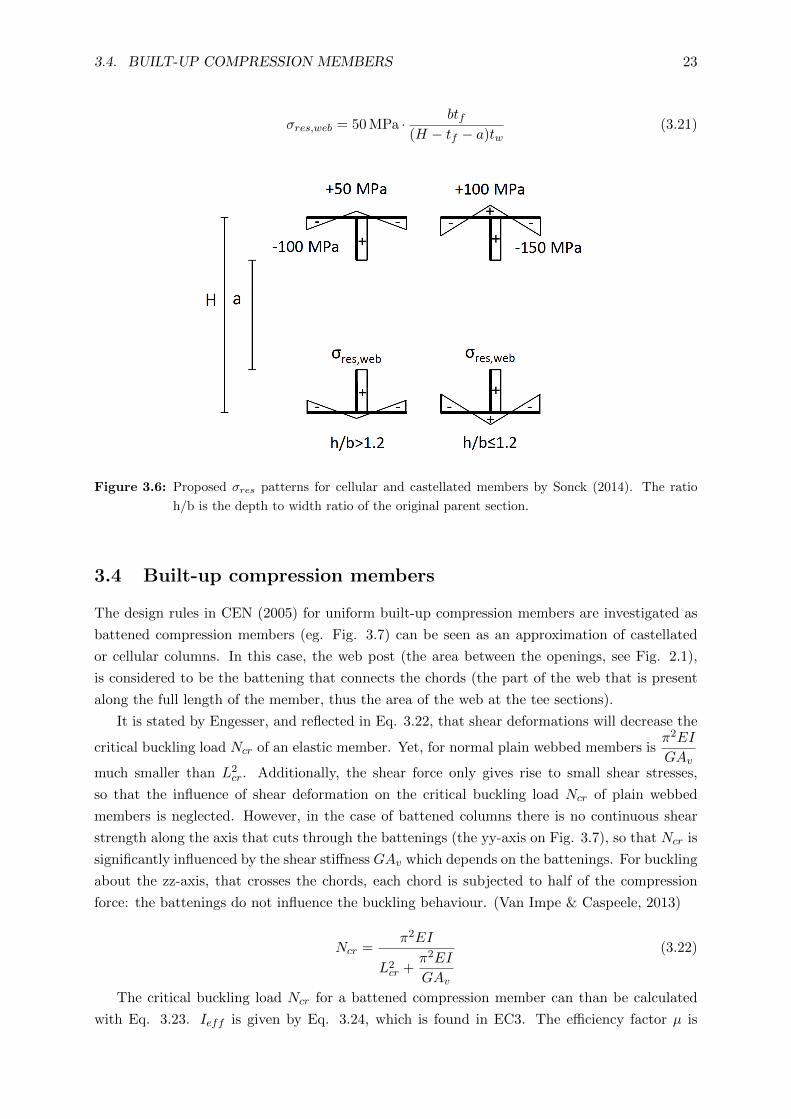
residual stresses in the web σres,web is given by Eq. 3.21. The proposed residual stress pattern
is displayed in Fig. 3.6 and is introduced as such along the full length of the member.
3.4. BUILT-UP COMPRESSION MEMBERS 23
σres,web = 50 MPa · btf(H − tf − a)tw
(3.21)
Figure 3.6: Proposed σres patterns for cellular and castellated members by Sonck (2014). The ratio
h/b is the depth to width ratio of the original parent section.
3.4 Built-up compression members
The design rules in CEN (2005) for uniform built-up compression members are investigated as
battened compression members (eg. Fig. 3.7) can be seen as an approximation of castellated
or cellular columns. In this case, the web post (the area between the openings, see Fig. 2.1),
is considered to be the battening that connects the chords (the part of the web that is present
along the full length of the member, thus the area of the web at the tee sections).
It is stated by Engesser, and reflected in Eq. 3.22, that shear deformations will decrease the
critical buckling load Ncr of an elastic member. Yet, for normal plain webbed members isπ2EI
GAvmuch smaller than L2
cr. Additionally, the shear force only gives rise to small shear stresses,
so that the influence of shear deformation on the critical buckling load Ncr of plain webbed
members is neglected. However, in the case of battened columns there is no continuous shear
strength along the axis that cuts through the battenings (the yy-axis on Fig. 3.7), so that Ncr is
significantly influenced by the shear stiffness GAv which depends on the battenings. For buckling
about the zz-axis, that crosses the chords, each chord is subjected to half of the compression
force: the battenings do not influence the buckling behaviour. (Van Impe & Caspeele, 2013)
Ncr =π2EI
L2cr +
π2EI
GAv
(3.22)
The critical buckling load Ncr for a battened compression member can than be calculated
with Eq. 3.23. Ieff is given by Eq. 3.24, which is found in EC3. The efficiency factor µ is

24 CHAPTER 3. FLEXURAL BUCKLING OF COLUMNS
Figure 3.7: Example of a laced (left) and battened compression member (right) (extracted from Van
Impe and Caspeele (2013))
determined as in Fig. 3.8. 1/(GAv) is determined as in Eq. 3.25, found in Van Impe and
Caspeele (2013). In EC3 (CEN, 2005) it is given as the shear stiffness Sv, but the equations are
essentially the same.
Ncr =π2EIeff
L2cr +
π2EIeffGAv
(3.23)
Ieff = 0.5h20Ach + 2µIch (3.24)
Ach cross-sectional area of the chord
Ich moment of inertia of one chord about its own centroid
h0 distance between the centroids of the chords
a′ distance between the centroids of the battenings
Ib moment of inertia of one battening
Ieff effective second moment of area of the built-up member
1
GAv=a′
12
(h0nEIb
+a′
2EIch
)(3.25)
It will be verified in section 6.2.1 whether the strong-axis critical buckling load Ncr of cellular
and castellated members can be calculated with Eq. 3.23. The tee sections are then considered
to be the chords, so that Ach and Ich are given by Eq. 3.26 and Eq. 3.28. Note that in these
equations a stands for the height of the opening (as defined in Fig. 6.1), whereas a′ is the

3.5. MAJOR-AXIS FLEXURAL BUCKLINGOF CELLULAR AND CASTELLATED COLUMNS 25
Figure 3.8: Efficiency factor µ (extracted from EC3 (CEN, 2005)).
distance between the centroids of the battenings, thus the distance between the centroids of the
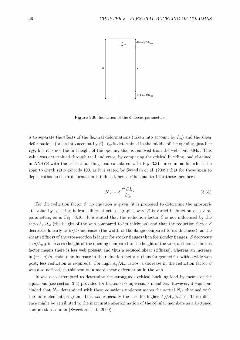
web posts. y (Eq. 3.27) is the location of the centroid of the chords, as indicated in Fig. 3.9.
The distance between the centroids of the chords h0 is equal to a+ 2y. The moment of inertia
of the battening (thus the web post) is given for cellular members by Eq. 3.29: an equivalent
opening with width 0.45a is assumed, so that the width of the web post is equal to w + 0.55a.
This equivalent opening is the same as used by Lawson and Hicks (2011) in chapter 4. The
moment of inertia of the battening (thus the web post) is given for castellated members by Eq.
3.30: an equivalent opening with width 0.5l0 = 0.5(2c+w) is assumed, so that the width of the
web post is equal to w + c+ w/2. This equivalent opening is the same as in chapter 4.
Ach =A2T
2= btw +
H − tf − a2
(3.26)
y =btfhweb + twh
2web/2
btf + twhweb(3.27)
Ich =bt3f12
+ btf (hweb − y)2 +twh
3web
12+ twhweb(
hweb2− y)2 (3.28)
Ib,cell =tw(w + 0.55a)3
12(3.29)
Ib,cast =tw(w + c+ w/2)3
12(3.30)
3.5 Major-axis flexural buckling of cellular and castellated columns
To the best of the authors knowledge, only two publications exist on the topic of strong-axis elas-
tic buckling: one on cellular columns by Sweedan et al. (2009) and one on castellated columns by
El-Sawy, Sweedan, and Martini (2009). As they are published by the same group of researchers,
the research is executed in a similar way.
3.5.1 Identification of the buckling capacity of axially loaded cellular columns
(Sweedan et al., 2009)
In Sweedan et al. (2009), a reduction factor β is proposed to determine the major-axis critical
buckling load of cellular columns. It is applied as in Eq. 3.31. The idea behind this equation
26 CHAPTER 3. FLEXURAL BUCKLING OF COLUMNS
(H-‐tf-‐a)/2=hweb
a
(H-‐tf-‐a)/2=hweb
y
H
Figure 3.9: Indication of the different parameters.
is to separate the effects of the flexural deformations (taken into account by Ieq) and the shear
deformations (taken into account by β). Ieq is determined in the middle of the opening, just like
I2T , but it is not the full height of the opening that is removed from the web, but 0.84a. This
value was determined through trail and error, by comparing the critical buckling load obtained
in ANSYS with the critical buckling load calculated with Eq. 3.31 for columns for which the
span to depth ratio exceeds 100, as it is stated by Sweedan et al. (2009) that for those span to
depth ratios no shear deformation is induced, hence β is equal to 1 for those members.
Ncr = βπ2EIeqL2cr
(3.31)
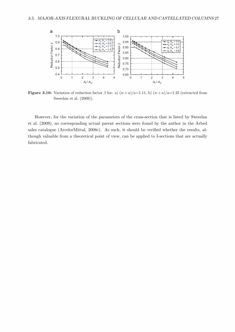
For the reduction factor β, no equation is given: it is proposed to determine the appropri-
ate value by selecting it from different sets of graphs, were β is varied in function of several
parameters, as in Fig. 3.10. It is stated that the reduction factor β is not influenced by the
ratio hw/tw (the height of the web compared to its thickness) and that the reduction factor β
decreases linearly as bf/tf increases (the width of the flange compared to its thickness), as the
shear stiffness of the cross-section is larger for stocky flanges than for slender flanges. β decreases
as a/hweb increases (height of the opening compared to the height of the web, an increase in this
factor means there is less web present and thus a reduced shear stiffness), whereas an increase
in (w+ a)/a leads to an increase in the reduction factor β (thus for geometries with a wide web
post, less reduction is required). For high Af/Aw ratios, a decrease in the reduction factor β
was also noticed, as this results in more shear deformation in the web.
It was also attempted to determine the strong-axis critical buckling load by means of the
equations (see section 3.4) provided for battened compressions members. However, it was con-
cluded that Ncr determined with these equations underestimates the actual Ncr obtained with
the finite element program. This was especially the case for higher Af/Aw ratios. This differ-
ence might be attributed to the inaccurate approximation of the cellular members as a battened
compression column (Sweedan et al., 2009).
3.5. MAJOR-AXIS FLEXURAL BUCKLINGOF CELLULAR AND CASTELLATED COLUMNS 27
Figure 3.10: Variation of reduction factor β for: a) (w+a)/a=1.11, b) (w+a)/a=1.25 (extracted from
Sweedan et al. (2009)).
However, for the variation of the parameters of the cross-section that is listed by Sweedan
et al. (2009), no corresponding actual parent sections were found by the author in the Arbed
sales catalogue (ArcelorMittal, 2008c). As such, it should be verified whether the results, al-
though valuable from a theoretical point of view, can be applied to I-sections that are actually
fabricated.
28 CHAPTER 3. FLEXURAL BUCKLING OF COLUMNS
Chapter 4
Additional deflection due to the
openings in the web
In several sources, mentioned below, approximate formula are given to determine the additional
deflection that occurs due to the presence of openings in the web in perforated beams. In these
formula, the ratio of the additional deflection δadd to the pure bending deflection δb is expressed
as a function of the number of openings n, the length of the member L, the height of the member
H, the effective length of the opening `eff , the height of the opening d0=a and some correction
factors (see Eq. 4.4 and 4.5). Consequently, the geometry of the openings is taken into account.
The total deflection of the beam can thus be determined as in Eq. 4.1 (based on Eq. 4.6):
δtot = δb + δadd =
(1 + 0.7nk0
`effd0LH
)δb (4.1)
Ieq,y =Iy(
1 + 0.7nk0`effd0LH
) (4.2)
The bending deflection is regardless of the load case expressed as a function of the strong-axis
moment of inertia Iy (see eg. Eq. 4.14 for the deflection of a beam subjected to a point load in
the middle), so that essentially an equivalent moment of inertia about the strong axis (Eq. 4.2)
is proposed to take the presence of the openings in the beam into account. It will be verified in
section 6.2 of chapter 6 whether this equivalent moment of inertia can be used to numerically
determine the strong-axis critical buckling load Ncr of cellular and castellated columns.
4.1 Approximate formula
In annex N of ENV3, the European pre-standard of Eurocode 3 (CEN, 1998), it is specified that
”the vertical deflection of a beam with multiple openings should be determined starting from
the total bending and shear deformation of the plain webbed beam, plus the additional defor-
mation due to the presence of the openings”. This additional deformation should be determined
considering (CEN, 1998):
• the effect of global bending on the total deformation of the perforated beam,
• the effect of local bending deformation of the tee sections,
29

30 CHAPTER 4. ADDITIONAL DEFLECTION
• the effect of local bending deformation of the web posts,
• the effect of shear deformation of the tee sections,
• the effect of shear deformation of the web posts.
The CTICM (2006), Centre Technique Industriel de la Construction Metallique, offers equations
to calculate the contribution of each of these effects separately for cellular members. To do this,
the perforated beam is subdivided into several types of panels, as can be seen in Fig. 4.1. A
”P” panel has the cross section of a plain webbed member and is typically found at the ends
of a cellular beam, or at those locations where a circular opening has been filled. A ”C” panel
forms the transition between the ”P” panels and the ”X” panels, of which the major part of the
beam is composed. Internal forces are used to determine the deflection and as the method is
based on a first order theory, axial forces have no effect. The CTICM developed these equations
for the company ArcelorMittal, which implemented them in its calculation tool ACB+ (since
version 2.00) for cellular beams. This calculation tool is freely available on their website and
also allows calculations of composite cellular beams. As the equations are quite complicated and
require the calculation of several additional parameters, they will not be further considered as
inspiration for the design rule.
Figure 4.1: Cellular beam broken down into panels of different types (extracted from CTICM (2006)).
Feldmann et al. (2006) propose an approximate empirical formula to calculate the additional
deflection δadd due to a single circular or rectangular opening (Eq. 4.3). The first two factors in
parentheses in Eq. 4.3 stand for the additional pure bending deflection due to the loss of stiffness
at the opening, whereas the last factor is added to decrease the contribution of the deflection in
low shear regions. The additional deflection is expressed relatively to the pure bending deflection
δb of the unperforated beam. The formula also takes the possibility of stiffened openings into
account by introducing the coefficient k0 which is equal to 1 for stiffened openings and equal
to 1.5 for unstiffened openings. `eff stands for the length of the opening and is taken equal to
0.5d0 for circular openings. H is the depth of the steel section and L stands for the length of
the beam.
δaddδb
= k0
(`effL
)(d0H
)(1− x
L
)for x ≤ 0.5L (4.3)
δaddδb
= 0.5nk0
(`effL
)(d0H
)(4.4)

4.2. PARAMETRIC STUDY 31
The formula is adapted for multiple openings by replacing(1− x
L
)with 0.5n. The factor 0.5
accounts for the combined effect of the distribution of moment and shear along the beam. n
represents the number of openings along the beam. It is pointed out that this is an approxi-
mate formula, which becomes more conservative for shorter openings. For those openings, the
Vierendeel deflections are less pronounced so that the formula predicts a larger deflection than
will occur in reality. It is also stated that the additional deflection due to the presence of the
openings generally lies between 10% and 15%.
δaddδb
= k0
(`effL
)(d0H
)(1− x
L
)for x ≤ 0.5L (4.5)
δaddδb
= 0.7nk0
(`effL
)(d0H
)(4.6)
Eq. 4.3 is also found in Lawson and Hicks (2011), but as Eq. 4.5. However, `eff is taken
equal to 0.45d0 for circular openings in this publication. Also the adaptation of the formula for
multiple openings is different, as(1− x
L
)is replaced by 0.7n (Eq. 4.6). The combined effect of
the distribution of moment and shear apparently has a larger impact according to Lawson and
Hicks (2011).
Neither Lawson nor Feldmann mention castellated beams, which have hexagonal openings. It
is assumed that for those openings `eff should also be reduced as is the case for circular openings.
In a preliminary document that offers a design method for composite and non-composite beams
with large web openings for the Eurocode hexagonal openings are mentioned and it is specified
that `eff should be taken equal to 0.5`0, in which `0 stands for the total length of the hexagonal
opening. However it is stated in the document that this value should still be confirmed by
experiments. In the same document it is also specified that `eff = 0.45d0 for circular openings,
as prescribed by Lawson and Hicks (2011).
As it is quite unclear what should be taken as the length of the opening for cellular members
and as the coefficient to account for the combined effect of the distribution of moment and shear
along the beam, a small parametric study is conducted to shed some light on the problem. In
this study, both castellated and cellular members will be considered, as the strong-axis flexural
buckling will be studied later for both castellated and cellular members.
4.2 Parametric study
4.2.1 Parent sections
The same parent sections as in the PhD of Sonck (2014) are chosen, as they will be used to
study the strong-axis flexural buckling. Their specifications can be found in table 6.1. They
were chosen from the available parent sections in the ArcelorMittal sales catalogue (ArcelorMittal
(2008c)), and thus considered to be representative of regularly used sections. The IPE300 and
IPE600 cover the normal application area, and of the wide flange sections, HEA and HEM are
selected to have the largest possible variation of section properties. To obtain a web height
hweb = h − 2tf that is as similar as possible for all the parent sections, HE320A, HE650A,
HE320M and HE650M are selected.

32 CHAPTER 4. ADDITIONAL DEFLECTION
Table 4.1: Dimensions of the considered parent sections.
Section h b tw tf
name [mm] [mm] [mm] [mm]
IPE300 300 150 7.1 10.7
IPE600 600 220 12.0 19.0
HE320A 310 300 9.0 15.5
HE650A 640 300 13.5 26.0
HE320M 359 309 21.0 40.0
HE650M 668 305 21.0 40.0
For each parent section, three configurations are considered for the cellular members: one
with large openings and small web posts, one with small openings and large web posts and a
configuration in between (the web post is the area between the openings, its width is referred
to as w as can be seen in Fig. 6.1). In the brochure of ArcelorMittal (2008a) for cellular beams,
ranges of the opening sizes are proposed for two objectives. Optimisation of the height/weight
ratio leads to large openings and small web posts and of this range the largest opening, a = 1.3h
(w = 0.1a), is retained. Optimisation of the load/weight ratio leads to smaller openings, and of
this range the smallest is retained: a = 0.8h (w = 0.7a). For the configuration in between, the
objective was to combine the largest opening size and the largest width of the web post. However,
in the same brochure constraints for the geometry are also prescribed and this configuration does
not comply with Eq. 2.10. To fulfil the geometrical constraints mentioned in part 2.4, the only
possible factor for w to comply with a = 1.3h is 0.1. To keep both w and a as large as possible
fa is taken equal to 1.0 and fw is taken equal to 0.7. For these values all the constraints are
fulfilled. This geometry falls within the limits of the optimisation load/weight and is thus a
reasonable geometry. The end web posts are twice the size of the web posts. The summary of
the considered geometries can be found in Table 4.2. Fig. 4.2 displays the different geometries
for the parent section IPE300.
Figure 4.2: Geometry 1, geometry 2 and geometry 3 of the cellular type for parent section IPE300.
Table 4.2: Summary of the considered configurations for cellular beams.
fa fw
geometry 1 1.3 0.1
geometry 2 0.8 0.7
geometry 3 1.0 0.7

4.2. PARAMETRIC STUDY 33
For the castellated members three configurations will be considered as well for each parent
section: one which has a typical Angelina configuration, one with a typical hexagonal config-
uration and one where the hexagons approximate rectangular openings (see Fig. 6.1 for an
indication of the general geometry of a castellated beam). For the Angelina configuration, com-
mon sections are listed in ArcelorMittal (2008b) and the equation of the curve of the opening is
taken equal to Eq. 4.7. Evaluating the derivation of this equation to x for x = b2 results in the
tangent of the inclined part of the opening. This is used to determine α (the opening angle of
the hexagonal opening, one of the three parameters that determine the geometry of a castellated
beam as specified in part 2.3), which is equal to 25.36◦. fH is taken equal to 1.5 and fw is taken
equal to 0.1.
y =(
0.5a
2
)· sin
[π
(x
b+
3
2
)]+a
4(4.7)
Figure 4.3: Indication of the parameters used in Eq. 4.7 (extracted from ArcelorMittal (2008b)).
Table 4.3: Summary of the considered configurations for the castellated beams.
fH α fw
geometry 1 1.5 25.36◦ 0.1
geometry 2 1.5 60◦ 0.3
geometry 3 1.5 80◦ 0.5
A regular hexagon has an angle α = 60◦, and for this configuration fH is taken equal to 1.5
and fw = 0.3. For the configuration that approximates rectangular openings, α is taken equal
to 80◦, fH = 1.5 and fw = 0.5. A summary of the different geometries can be found in Table
4.3. Fig. 4.4 displays the different geometries for the parent section IPE300.
Figure 4.4: Geometry 1, geometry 2 and geometry 3 of the castellated type for parent section IPE300.
For the three geometries of both the cellular and castellated beams, six lengths are considered.

34 CHAPTER 4. ADDITIONAL DEFLECTION
They are obtained by varying the number of openings: n=8, 20, 40, 60, 80 or 100. This range
for the number of openings n leads to a maximum member length of 114.9 m for geometry 3
of the cellular type for parent section HE650M. This is an unrealistic length for a beam, but
is considered anyway to obtain the same range of slendernesses as will be considered in the
parametric study for the determination of the strong-axis flexural buckling behaviour. Thus 216
different geometries are considered in total. For all of these, the different geometric constraints
are checked. All three configurations for the castellated members fulfill the constraints mentioned
in part 2.4. However, not all of the configurations for the cellular members comply with all the
constraints, as can be seen in Table 4.4. Nevertheless, the parametric study is conducted for all
the configurations, keeping in mind that some of the results only have theoretical meaning.
Table 4.4: Summary of the different considered geometries of the cellular type.
a w H does not fulfil
IPE300 geometry 1 0.390 0.039 0.486
geometry 2 0.240 0.168 0.374
geometry 3 0.300 0.210 0.396
IPE600 geometry 1 0.780 0.078 0.980
geometry 2 0.480 0.336 0.760
geometry 3 0.600 0.420 0.803
HE320A geometry 1 0.403 0.040 0.502 Eq. 2.16
geometry 2 0.248 0.174 0.387
geometry 3 0.310 0.217 0.409 Eq. 2.16
HE650A geometry 1 0.832 0.083 1.046
geometry 2 0.512 0.358 0.811
geometry 3 0.640 0.448 0.857
HE320M geometry 1 0.467 0.047 0.583 Eq. 2.16 and Eq. 2.17
geometry 2 0.287 0.201 0.450
geometry 3 0.359 0.251 0.476 Eq. 2.16 and Eq. 2.17
HE650M geometry 1 0.868 0.087 1.092
geometry 2 0.534 0.374 0.847
geometry 3 0.668 0.468 0.895
4.2.2 Determination of the additional deflection
The approximate formulas predict the additional deflection of perforated beams due to the
presence of the openings, compared to the same beam without openings. The pure bending
deflection of the member is determined with the program Abaqus (Dassault Systemes, 2014)
for two load cases: a line load of 25 kN/m and a point load of 1 kN that acts in the middle of
the beam. The values of the loads were chosen arbitrarily, as it is the ratio δadd/δb that will
be evaluated. This is done for both the beam with and without openings. Only beams with
unstiffened openings are considered, hence k0 equals 1.5. Two equations will be compared to
what is obtained in Abaqus:

4.2. PARAMETRIC STUDY 35
Table 4.5: Summary of the different considered geometries of the castellated type.
α w H
IPE300 geometry 1 25.36 0.070 0.450
geometry 2 60 0.074 0.450
geometry 3 80 0.053 0.450
IPE600 geometry 1 25.36 0.141 0.900
geometry 2 60 0.148 0.900
geometry 3 80 0.106 0.900
HE320A geometry 1 25.36 0.073 0.465
geometry 2 60 0.077 0.465
geometry 3 80 0.055 0.465
HE650A geometry 1 25.36 0.150 0.960
geometry 2 60 0.158 0.960
geometry 3 80 0.113 0.960
HE320M geometry 1 25.36 0.084 0.539
geometry 2 60 0.089 0.539
geometry 3 80 0.063 0.539
HE650M geometry 1 25.36 0.157 1.002
geometry 2 60 0.165 1.002
geometry 3 80 0.118 1.002
For cellular beams
• Eq. 4.8 proposed by Feldmann et al. (2006), for which `eff is taken equal to 0.5d0, leading
to Eq. 4.9δaddδb
= 0.5nk0
(`effL
)(d0H
)(4.8)
δaddδb
= 0.375nd20HL
(4.9)
• Eq. 4.10 proposed by Lawson and Hicks (2011), for which `eff is taken equal to 0.45d0,
leading to Eq. 4.11δaddδb
= 0.7nk0
(`effL
)(d0H
)(4.10)
δaddδb
= 0.47nd20HL
(4.11)
For castellated beams
Neither Feldmann nor Lawson mention hexagonal openings. In a preliminary document that
offers a design method for composite and non-composite beams with large web openings for
the Eurocode hexagonal openings are however mentioned and it is specified that `eff should be
taken equal to 0.5`0, in which `0 stands for the total length of the hexagonal opening (w+2c).
d0 stands for the height of the opening and is equal to a. This results in Eq. 4.13.
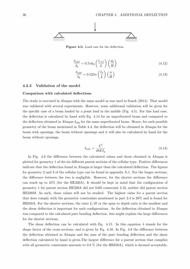
36 CHAPTER 4. ADDITIONAL DEFLECTION
Figure 4.5: Load case for the deflection.
δaddδb
= 0.7nk0
(`effL
)(d0H
)(4.12)
δaddδb
= 0.525n
(`0L
)( aH
)(4.13)
4.2.3 Validation of the model
Comparison with calculated deflections
The study is executed in Abaqus with the same model as was used in Sonck (2014). That model
was validated with several experiments. However, some additional validation will be given for
the specific case of a beam loaded by a point load in the middle (Fig. 4.5). For this load case,
the deflection is calculated by hand with Eq. 4.14 for an unperforated beam and compared to
the deflection obtained in Abaqus δabq for the same unperforated beam. Hence, for each possible
geometry of the beam mentioned in Table 4.4, the deflection will be obtained in Abaqus for the
beam with openings, the beam without openings and it will also be calculated by hand for the
beam without openings.
δcalc =L3
48EIy(4.14)
In Fig. 4.6 the difference between the calculated values and those obtained in Abaqus is
plotted for geometry 1 of the six different parent sections of the cellular type. Positive differences
indicate that the deflection found in Abaqus is larger than the calculated deflection. The figures
for geometry 2 and 3 of the cellular type can be found in appendix A.1. For the longer sections,
the difference between the two is negligible. However, for the shorter sections the difference
can reach up to 45% (for the HE320A). It should be kept in mind that the configuration of
geometry 1 for parent section HE320A did not fulfil constraint 2.16, neither did parent section
HE320M. As such, these values will not be studied. The highest value for a parent section
that does comply with the geometric constraints mentioned in part 2.4 is 28% and is found for
HE650A. For the shorter sections, the ratio L/H or the span to depth ratio is the smallest and
the shear deflection is important for such configurations. As the deflection obtained in Abaqus
was compared to the calculated pure bending deflection, this might explain the large differences
for the shorter sections.
The shear deflection can be calculated with Eq. 4.15. In this equation λ stands for the
shape factor of the cross sections, and is given by Eq. 4.16. In Fig. 4.8 the difference between
the deflection obtained in Abaqus and the sum of the pure bending deflection and the shear
deflection calculated by hand is given.The largest difference for a parent section that complies
with all geometric constraints amounts to 3.8 % (for the HE650A), which is deemed acceptable,

4.2. PARAMETRIC STUDY 37
0 20 40 60 80 100Length [m]
0
10
20
30
40
50
%di
ffer
ence
betw
eenδ abq
andδ calc
Geometry 1 (cellular type): fa = 1.3 and fw=0.1
IPE300IPE600HE320MHE650MHE320AHE650A
Figure 4.6: Difference between the calculated bending deflection δcalc and the deflection obtained in
Abaqus δabq in % for plain-webbed beams subjected to a point load in the middle.
especially as these ’larger’ differences only arise for the shortest profiles. As for the validation
only plain-webbed members are considered, to be able to compare the deflection obtained in
Abaqus with calculations by hand, only members defined by geometries of the cellular type
found in Table 4.4 are considered. This means that only the increased height is found back in
the plain-webbed members. Hence, the model is also validated for the castellated members as
approximately the same range in increased height H is found as for the cellular members (see
Table 4.5).
δshear =
∫ `/2
0
λ
GAVzdx (4.15)
λ =ASmaxe0Iy
(4.16)
with:
G shear modulus
A total cross section of the profile
Smax static moment of the cross section above the neutral line
e0 width of the profile at z=0
Iy moment of inertia around the y-axis
Smax = btfH − tf
2+ tw
(H − tf )2
8(4.17)
Iy =tw(H − tf )3
12+ 2
[bt3f12
+ btf
(H − tf
2
)2]
(4.18)

38 CHAPTER 4. ADDITIONAL DEFLECTION
Figure 4.7: Definition of the axes (extracted from Sonck (2014)).
0 20 40 60 80 100Length [m]
−1
0
1
2
3
4
5
6
7
%di
ffer
ence
betw
eenδ abq
andδ calc
Geometry 1 (cellular type): fa = 1.3 and fw = 0.1
IPE300IPE600HE320MHE650MHE320AHE650A
Figure 4.8: Difference between the deflection obtained in Abaqus δabq and the calculated bending and
shear deflection of plain-webbed members.

4.2. PARAMETRIC STUDY 39
To be certain that the deviations are not due to the model in Abaqus, an analysis was also run
for a different element type. Shell elements were used for the model and in Abaqus a distinction
is made between thin shell problems and thick shell problems. For thin shell problems it is
assumed that transverse shear deformations are negligible, whereas they are important in thick
shell problems. As the deviations occur for the profiles with the smallest span to depth ratios,
for which it is known that the shear deformation might exceed the bending deformation, it is
concluded that this is a case where transverse shear deformations are important. For those, the
element ’S8R’ is advised, which is exactly the element used in the model. An analysis was also
made with the thin shell element ’S4R5’, but this resulted in the same deflection as found for
the analysis with the ’S8R’ element.
Comparison with the program ACB+ of ArcelorMittal
Figure 4.9: The program ACB+ of ArcelorMittal.
The results found in Abaqus for the cellular members were also compared to the results found
in the program ACB+ of ArcelorMittal. This program, of which Fig. 4.9 is a screenshot, uses
the equations prescribed by the CTICM (2006) to predict the deflection. As this is a practical
program, several additional constraints arise such as a minimum length of 5 m and a maximum
length of 50 m. The minimum width of the web post is restricted to 50 mm. This constraint was
disregarded during the numerical investigation as it would exclude geometry 1 of the cellular
type for the smaller parent sections (IPE300, HE320A and HE320M). In the program however
it is applied, so that for those parent sections no comparison could be made for geometry 1.
For geometry 3 applied to parent sections HE320M and HE320A, constraint 2.16 is not fulfilled.
Hence, for this geometry no comparison could be made either.
∆ACB+ =
(δabqδACB+
− 1
)· 100% (4.19)
Of the remaining configurations two were chosen for each case and each parent section: one

40 CHAPTER 4. ADDITIONAL DEFLECTION
with the largest feasible length and one with the smallest feasible length. The results can be
found in Table 4.6 and Table 4.7. The largest difference, obtained with Eq. 4.19, between
the values obtained in Abaqus and ACB+ occurs for configuration c1 of parent section IPE600
and amounts to 10.44% (see Table 4.7). A negative difference indicates that the deflection
obtained in ACB+ exceeds the one obtained in Abaqus. Hence, for the larger profiles, the
deflection obtained in ACB+ overestimates the deflection for long beams, and underestimates
it for shorter beams. For the smaller parent sections, all the configurations of geometry 2 were
examined in ACB+ and compared to the values obtained in Abaqus for the deflection. Fig. 4.10
displays the differences between the two. In the graph no real pattern is obvious so that it is
concluded that the differences are irregular.
Table 4.6: Comparison between the results from Abaqus and ACB+ for the smaller parent sections.
L [m] δabq [m] δACB+ [m] ∆ACB+ [%]
IPE300 geometry 2 c8 8.664 -0.00054 -0.00054 0.11
c12 41.304 -0.05441 -0.05455 -0.26
geometry 3 c14 10.830 -0.00096 -0.00097 -0.01
c17 41.430 -0.05011 -0.05043 -0.63
HE320M geometry 2 c8 10.368 -0.00011 -0.00011 -2.30
c12 49.427 -0.01061 -0.01100 -3.55
HE320A geometry 2 c8 8.953 -0.00023 -0.00022 4.53
c12 42.681 -0.02207 -0.02165 1.94
0 10 20 30 40 50 60Length [m]
−6
−4
−2
0
2
4
6
∆ACB
+[%
]
Geometry 2 (cellular type): fa = 0.8 and fw=0.7
IPE300HE320MHE320A
Figure 4.10: ∆ACB+ for the smaller parent sections (geometry 2).

4.2. PARAMETRIC STUDY 41
Table 4.7: Comparison between the results from Abaqus and ACB+ for the larger parent sections.
L [m] δabq [m] δACB+ [m] ∆ACB+ [%]
IPE600 geometry 1 c1 7.098 -0.00006 -0.00005 10.44
c3 34.554 -0.00195 -0.00196 -0.56
geometry 2 c7 7.536 -0.00004 -0.00004 3.84
c10 49.968 -0.00842 -0.00861 -2.17
geometry 3 c13 9.420 -0.00007 -0.00007 4.12
c15 42.060 -0.00465 -0.00481 -3.37
HE650M geometry 1 c1 7.902 -0.00003 -0.00003 6.53
c3 38.470 -0.00087 -0.00089 -2.50
geometry 2 c7 8.390 -0.00002 -0.00002 5.41
c9 37.461 -0.00113 -0.00118 -4.32
geometry 3 c13 10.488 -0.00003 -0.00003 2.65
c15 46.827 -0.00201 -0.00210 -4.52
HE650A geometry 1 c1 7.571 -0.00005 -0.00005 7.16
c3 36.858 -0.00128 -0.00128 0.00
geometry 2 c7 8.038 -0.00003 -0.00003 5.92
c9 35.891 -0.00165 -0.00167 -1.38
geometry 3 c13 10.048 -0.00005 -0.00004 6.77
c15 44.864 -0.00293 -0.00300 -2.50
4.2.4 Results
Deflection of a beam subjected to a point load
The deflection obtained in Abaqus for a cellular beam subjected to a point load in the middle
is compared to two equations that approximately predict the additional deflection of the beam
due to the presence of the openings: Eq. 4.21 proposed by Feldmann et al. (2006) and Eq.
4.22 proposed by Lawson and Hicks (2011). The ratio (δadd/δb)abq is obtained as in Eq. 4.20.
First, the deflections for the different parent sections will be compared, after which a comparison
will be made of the ratio δadd/δb between the different geometries and for the different parent
sections. (δaddδb
)abq
=δopenings,abq − δno openings,abq
δno openings,abq(4.20)
(δaddδb
)Feldmann
= 0.375nd20HL
(4.21)
(δaddδb
)Lawson
= 0.47nd20HL
(4.22)
When comparing the different parent sections for a specific geometry, it is expected that
the deflection δopenings,abq of the smaller parent sections (IPE300, HE320M, HE320A) will be
larger than the deflection of the larger parent sections (IPE600, HE650M, HE650A) as these
have a larger height and thus more resistance to bending. Indeed, for a length of e.g. 40 m, the

42 CHAPTER 4. ADDITIONAL DEFLECTION
deflections of the smaller parent sections are larger than those of the larger parent sections (Fig.
4.11). This also holds true for the other considered geometries, as can be seen in Fig. 4.12 and
in Fig. 4.13. The largest deflection is found for the IPE300 section as the bending resistance
of the HE320M and HE320A sections is larger due to the contribution of the thicker flanges to
the moment of inertia about the strong axis. The contribution of the flanges to the moment of
inertia about the y-axis is larger than the contribution of the web.
Figures 4.11 and 4.12 represent the extreme geometries of the largest opening paired with
the smallest width w of the web post (geometry 1) and the smallest opening paired with the
largest width w of the web post (geometry 2). For geometry 1, due to the larger openings and
smaller web posts, less material is available to take on the shear stresses so that larger shear
deformations are expected (Fig. 4.14a displays geometry 1 for an IPE300). For geometry 2 on
the other hand (Fig. 4.14b displays geometry 2 for an IPE300), more material is available so that
it could be expected that the deflections would be larger for geometry 1 than for geometry 2.
However, for geometry 1, the height has increased with a factor 1.62 whereas the height increase
for geometry 2 is only 1.25. This increase has a significant influence on the moment of inertia
about the y-axis, as the third and second powers of this height appear in Eq. 4.18. Hence the
sections from geometry 1 have a larger bending resistance, leading to smaller deflections than
those obtained for geometry 2. The deflections obtained in Abaqus for geometry 3 (Fig. 4.13)
are similar to those found for geometry 2. As the combination of fa = 1.0 and fw = 0.7 leads
to large openings and wide web posts, the members with this geometry are the longest. The
height has increased with a factor 1.32, so that the deflections found for geometry 2 are slightly
larger than those found for members of geometry 3 of a similar length.
(a) Geometry 1. (b) Geometry 2.
Figure 4.14: IPE300: example of the two extreme geometries.
Figures 4.15a and 4.15b display the ratio (δadd/δb)abq obtained in Abaqus for geometry 2
and geometry 3 of parent section IPE300. Also the proposed equations Eq. 4.9 and Eq. 4.11 to
determine the additional deflection are displayed in the figures. The additional deflection δadd
due to the presence of the openings is larger for geometry 3 and at most equal to 40 % of the
bending deflection δb. For both geometries a peak is noted for the first configuration, which is the
shortest. Hence also the span to depth ratio is the smallest. As this peak exceeds the proposed
equations, they are unsafe for smaller span to depth ratios. For the second configuration, the
span to depth ratio is 23 and 27 for geometry 2 and geometry 3 respectively.
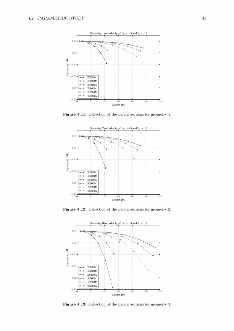
4.2. PARAMETRIC STUDY 43
0 20 40 60 80 100 120
Length [m]
−0.10
−0.08
−0.06
−0.04
−0.02
0.00
δ openings,abq
[m]
Geometry 1 (cellular type): fa = 1.3 and fw = 0.1
IPE300HE320MHE320AIPE600HE650MHE650A
Figure 4.11: Deflection of the parent sections for geometry 1.
0 20 40 60 80 100 120
Length [m]
−0.10
−0.08
−0.06
−0.04
−0.02
0.00
δ openings,abq
[m]
Geometry 2 (cellular type): fa = 0.8 and fw = 0.7
IPE300HE320MHE320AIPE600HE650MHE650A
Figure 4.12: Deflection of the parent sections for geometry 2.
0 20 40 60 80 100 120
Length [m]
−0.10
−0.08
−0.06
−0.04
−0.02
0.00
δ openings,abq
[m]
Geometry 3 (cellular type): fa = 1.0 and fw = 0.7
IPE300HE320MHE320AIPE600HE650MHE650A
Figure 4.13: Deflection of the parent sections for geometry 3.

44 CHAPTER 4. ADDITIONAL DEFLECTION
For beams with a higher span to depth ratio, the additional deflection δadd reaches a value
of approximately 5% for geometry 2 and 8% for geometry 3 of the bending deflection δb. For
geometry 2, (δadd/δb)Feldmann predicts 14% whereas (δadd/δb)Lawson predicts 18%. For geometry
3, (δadd/δb)Feldmann predicts 17% whereas (δadd/δb)Lawson predicts 21%. For these span to depth
ratios, Eq. 4.9 and Eq. 4.11 are thus safe.
It was also stated by Feldmann et al. (2006) that Eq. 4.9 is more conservative for shorter
openings. This can be observed in Fig. 4.15a, where there is a larger difference between the
proposed equations and the actually obtained δadd/δb in Abaqus than in Fig. 4.15b, as for
geometry 2 the diameter of the openings d0 equals 0.24 m and for geometry 3 0.30 m (cf. Table
4.4) . Additionally, (δadd/δb)Feldmann and (δadd/δb)Lawson predict a larger deflection for geometry
3, as they essentially are determined as the surface area of equivalent rectangular openings
(n · 0.5d0 · d0) divided by the surface area of the web (LH) multiplied with some correction
factors. (δadd/δb)Feldmann and (δaddδb)Lawson remain relatively constant for increasing lengths,
a behaviour that is reflected by (δadd/δb)abq.
0 20 40 60 80 100 120
Length [m]
0.0
0.1
0.2
0.3
0.4
0.5
0.6
δ add/δb
Geometry 2 (cellular type): fa = 0.8 and fw = 0.7
IPE300(δadd/δb)Feldmann
(δadd/δb)Lawson
(a) Geometry 2.
0 20 40 60 80 100 120
Length [m]
0.0
0.1
0.2
0.3
0.4
0.5
0.6
δ add/δb
Geometry 3 (cellular type): fa = 1.0 and fw = 0.7
IPE300(δadd/δb)Feldmann
(δadd/δb)Lawson
(b) Geometry 3.
Figure 4.15: (δadd/δb)abq for parent section IPE300.
Figures 4.16a and 4.16b display the ratio (δadd/δb)abq obtained in Abaqus for geometry 2
and geometry 3 of parent section HE320M. Also for the parent section with the thicker flanges
geometry 3 results in the largest additional deflection. Again the peak is noted for the first
configurations, that have a span to depth ratio of 10 and 12 for geometry 2 and geometry
3 respectively. The span to depth ratio of the second configurations is equal to 23 and 27
respectively, and for those and larger span to depth ratios Eq. 4.9 and Eq. 4.11 are safe. This
is the same span to depth ratio that was found for parent section IPE300. For the larger span
to depth ratios, the additional deflection δadd due to the presence of the openings amounts
to 3.5% and 5% of the bending deflection δb for geometry 2 and geometry 3 respectively. For
geometry 2, (δadd/δb)Feldmann predicts 14% whereas (δadd/δb)Lawson predicts 18%. For geometry
3, (δadd/δb)Feldmann predicts 17% whereas (δadd/δb)Lawson predicts 21%. These are the exact
same values as were found for parent section IPE300, hence Eq. 4.9 and Eq. 4.11 do not depend
on the parent section, whereas (δadd/δb)abq does differ for the different parent sections.

4.2. PARAMETRIC STUDY 45
0 20 40 60 80 100 120
Length [m]
0.0
0.1
0.2
0.3
0.4
0.5
0.6δ add/δb
Geometry 2 (cellular type): fa = 0.8 and fw = 0.7
HE320M(δadd/δb)Feldmann
(δadd/δb)Lawson
(a) Geometry 2.
0 20 40 60 80 100 120
Length [m]
0.0
0.1
0.2
0.3
0.4
0.5
0.6
δ add/δb
Geometry 3 (cellular type): fa = 1.0 and fw = 0.7
HE320M(δadd/δb)Feldmann
(δadd/δb)Lawson
(b) Geometry 3.
Figure 4.16: (δadd/δb)abq for parent section HE320M.
Figures 4.17a and 4.17b display the ratio δadd/δb for geometry 2 and geometry 3 of parent
section HE650M. Again the peak is noted for the first configurations, that also have a span to
depth ratio of 10 and 12 for geometry 2 and geometry 3 respectively. For the longer configurations
the proposed equations are again safe. Their span to depth ratio is again equal to 23 and 27
respectively. This is the same span to depth ratio that was found for the parent sections IPE300
and HE320M. The additional deflection for the longer spans is about 5% for geometry 2 and
about 7% for geometry 3. (δadd/δb)Feldmann and (δadd/δb)Lawson again predict the same values
as were found for IPE300 and HE320M for the different geometries.
0 20 40 60 80 100 120
Length [m]
0.0
0.1
0.2
0.3
0.4
0.5
0.6
δ add/δb
Geometry 2 (cellular type): fa = 0.8 and fw = 0.7
HE650M(δadd/δb)Feldmann
(δadd/δb)Lawson
(a) Geometry 2.
0 20 40 60 80 100 120
Length [m]
0.0
0.1
0.2
0.3
0.4
0.5
0.6
δ add/δb
Geometry 3 (cellular type): fa = 1.0 and fw = 0.7
HE650M(δadd/δb)Feldmann
(δadd/δb)Lawson
(b) Geometry 3.
Figure 4.17: (δadd/δb)abq for parent section HE650M.
Figures 4.18a and 4.18b display geometry 1 for the smaller parent section IPE300 and
the larger parent section HE650M. Where there was sufficient safety between the actual ra-
tio (δadd/δb)abq and the proposed equations for geometry 2 and geometry 3 for span to depth
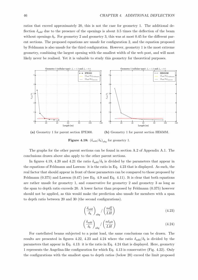
46 CHAPTER 4. ADDITIONAL DEFLECTION
ratios that exceed approximately 20, this is not the case for geometry 1. The additional de-
flection δadd due to the presence of the openings is about 3.5 times the deflection of the beam
without openings δb. For geometry 2 and geometry 3, this was at most 0.45 for the different par-
ent sections. The proposed equations are unsafe for configuration 2, and the equation proposed
by Feldmann is also unsafe for the third configuration. However, geometry 1 is the most extreme
geometry, combining the largest opening with the smallest width of the web post, and will most
likely never be realised. Yet it is valuable to study this geometry for theoretical purposes.
0 20 40 60 80 100 120
Length [m]
0
1
2
3
4
5
δ add/δb
Geometry 1 (cellular type): fa = 1.3 and fw = 0.1
IPE300(δadd/δb)Feldmann
(δadd/δb)Lawson
(a) Geometry 1 for parent section IPE300.
0 20 40 60 80 100 120
Length [m]
0
1
2
3
4
5
δ add/δb
Geometry 1 (cellular type): fa = 1.3 and fw = 0.1
HE650M(δadd/δb)Feldmann
(δadd/δb)Lawson
(b) Geometry 1 for parent section HE650M.
Figure 4.18: (δadd/δb)abq for geometry 1.
The graphs for the other parent sections can be found in section A.2 of Appendix A.1. The
conclusions drawn above also apply to the other parent sections.
In figures 4.19, 4.20 and 4.21 the ratio δadd/δb is divided by the parameters that appear in
the equations of Feldmann and Lawson: it is the ratio in Eq. 4.23 that is displayed. As such, the
real factor that should appear in front of these parameters can be compared to those proposed by
Feldmann (0.375) and Lawson (0.47) (see Eq. 4.9 and Eq. 4.11). It is clear that both equations
are rather unsafe for geometry 1, and conservative for geometry 2 and geometry 3 as long as
the span to depth ratio exceeds 20. A lower factor than proposed by Feldmann (0.375) however
should not be applied, as this would make the prediction also unsafe for members with a span
to depth ratio between 20 and 30 (the second configurations).(δaddδb
)abq
/
(nd20LH
)(4.23)
(δaddδb
)abq
/
(n`0a
LH
)(4.24)
For castellated beams subjected to a point load, the same conclusions can be drawn. The
results are presented in figures 4.22, 4.23 and 4.24 where the ratio δadd/δb is divided by the
parameters that appear in Eq. 4.13: it is the ratio in Eq. 4.24 that is displayed. Here, geometry
1 represents the Angelina-like configuration for which Eq. 4.13 is conservative (Fig. 4.22). Only
the configurations with the smallest span to depth ratios (below 20) exceed the limit proposed

4.2. PARAMETRIC STUDY 47
in the preliminary document for the Eurocode (0.525). Geometry 2 is the regular hexagonal
geometry, for which Eq. 4.13 is also conservative for larger span to depth ratios (Fig. 4.23). In
geometry 3 the openings are approximately rectangular. For this geometry not only the first
configurations exceed the proposed value, but also the second configurations (Fig. 4.24). The
proposed value is also less conservative. However, this is an extreme geometry that most likely
will not be fabricated in reality. Yet, it is still valuable to consider this geometry for theoretical
purposes.
0 20 40 60 80 100 120
Length [m]
0
1
2
3
4
5
6
7
8
δ add
δ b/nd
2 0
LH
Geometry 1 (cellular type): fa = 1.3 and fw = 0.1
IPE300IPE600HE320AHE650AHE320MHE650MFeldmannLawson
Figure 4.19: Cellular beam subjected to a point load: geometry 1.
0 20 40 60 80 100 120
Length [m]
0.0
0.2
0.4
0.6
0.8
1.0
1.2
1.4
1.6
δ add
δ b/nd
2 0
LH
Geometry 2 (cellular type): fa = 0.8 and fw = 0.7
IPE300IPE600HE320AHE650AHE320MHE650MFeldmannLawson
Figure 4.20: Cellular beam subjected to a point load: geometry 2.

48 CHAPTER 4. ADDITIONAL DEFLECTION
0 20 40 60 80 100 120
Length [m]
0.0
0.2
0.4
0.6
0.8
1.0
1.2
1.4
1.6
δ add
δ b/nd
2 0
LH
Geometry 3 (cellular type): fa = 1.0 and fw = 0.7
IPE300IPE600HE320AHE650AHE320MHE650MFeldmannLawson
Figure 4.21: Cellular beam subjected to a point load: geometry 3.
0 20 40 60 80 100 120 140 160 180
Length [m]
0.0
0.2
0.4
0.6
0.8
1.0
1.2
1.4
δ add
δ b/n` 0a
LH
Geometry 1 (castellated type):fH=1.5, α=25.36◦ and fw=0.1
IPE300IPE600HE320AHE650AHE320MHE650M
Figure 4.22: Castellated beam subjected to a point load: geometry 1.

4.2. PARAMETRIC STUDY 49
0 10 20 30 40 50 60 70 80
Length [m]
0.0
0.2
0.4
0.6
0.8
1.0
1.2
1.4
δ add
δ b/n` 0a
LH
Geometry 2 (castellated type): fH=1.5, α=60◦ and fw=0.3
IPE300IPE600HE320AHE650AHE320MHE650M
Figure 4.23: Castellated beam subjected to a point load: geometry 2.
0 10 20 30 40 50
Length [m]
0.0
0.5
1.0
1.5
2.0
2.5
3.0
3.5
4.0
δ add
δ b/n` 0a
LH
Geometry 3 (castellated type): fH=1.5, α=80◦ and fw=0.6
IPE300IPE600HE320AHE650AHE320MHE650M
Figure 4.24: Castellated beam subjected to a point load: geometry 3.

50 CHAPTER 4. ADDITIONAL DEFLECTION
Deflection of a perforated beam subjected to a lineload
Figures 4.25a and 4.25b display the additional deflection δadd due to the openings for a cellular
and castellated beam respectively. From the figures it can be deduced that the additional
deflection is smaller for the cellular beams than for the castellated ones. The peak for the first
configuration (with the smallest span to depth ratio) is also larger for the castellated beams. Yet,
apart from the peak for the first configuration, the proposed equations to predict the additional
deflection are more conservative for the castellated beams (Eq. 4.13) than for the cellular beams
(Eq. 4.9 and Eq. 4.11).
Figures 4.27, 4.28 and 4.29 display the ratio δadd/δb divided by the parameters that appear
in the equations of Feldmann and Lawson for the cellular beams: it is the ratio(δaddδb
)abq
/(nd20LH
)that is displayed. It is clear that also for a uniformly distributed load the safety of the proposed
equations for geometry 1 (the largest openings pared with the smallest width of the web post)
is small. Yet, this is an extreme geometry that will most likely not be fabricated in reality. The
equations are conservative for the second and third geometry, as long as the profile has a span
to depth ratio larger than 20 (the first configuration has a span to depth ratio smaller than 20
and thus exceeds both Eq.4.9 and Eq. 4.11: the additional deflection δadd due to the presence
of the openings is larger than what these equations predict).
Comparing these figures with figures 4.19, 4.20 and 4.21, where the same cellular beam is
subjected to a point load, it is clear that the displayed ratio(δaddδb
)abq
/(nd20LH
)is smaller for
beams subjected to a lineload than to a point load. As the peak is most likely due to increased
shear deformations for the profiles with small span to depth ratios, it is also suspected that
this difference is due to difference in shear force distribution: for a point load, the whole beam
is subjected to constant shear force. For a beam subjected to an uniformly distributed load
however, the shear force is not constant along the beam (Fig. 4.26). Hence, the additional
deflection is larger for the beam subjected to a point load.
Figures 4.30, 4.31 and 4.32 display the ratio δadd/δb divided by the parameters that appear
in Eq. 4.13: it is the ratio(δaddδb
)abq
/(n`0aLH
)that is displayed. Geometry 1 represents the
Angelina-like configuration for which Eq. 4.13 is conservative. Even the configurations with
the smallest span to depth ratios (below 20) have a(δaddδb
)abq
lower than what the preliminary
document for the Eurocode predicts. Geometry 2 is the regular hexagonal geometry, for which
Eq. 4.13 is conservative for larger span to depth ratios (exceeding 20). In geometry 3 the
openings are approximately rectangular. For this geometry not only the first configurations
exceed the proposed value, but also the second configurations. The proposed value is also less
conservative. However, this is an extreme geometry that most likely will not be fabricated in
reality. Yet, it is still valuable to consider this geometry for theoretical purposes.

4.2. PARAMETRIC STUDY 51
0 20 40 60 80 100 120
Length [m]
0.0
0.1
0.2
0.3
0.4
0.5
0.6δ add/δb
Geometry 2 (cellular type): fa = 0.8 and fw = 0.7
IPE300(δadd/δb)Feldmann
(δadd/δb)Lawson
(a) Cellular beam: geometry 2.
0 20 40 60 80 100 120
Length [m]
0.0
0.1
0.2
0.3
0.4
0.5
0.6
δ add/δb
Geometry 2 (castellated type): fH=1.5, α=60◦ and fw=0.3
IPE300Draft
(b) Castellated beam: geometry 2.
Figure 4.25: (δadd/δb)abq for parent section IPE300 subjected to a line load.
(a) due to an uniformly distributed load.
(b) due to a point load.
Figure 4.26: Shear force.
4.2.5 Conclusions
The proposed equations by Feldmann et al. (2006) (Eq. 4.25) and Lawson and Hicks (2011) (Eq.
4.26) to predict the additional deflection of cellular beams due to the presence of openings in the
web are conservative, as long as the span to depth ratio exceeds 20. For smaller span to depth
ratios the influence of the increased shear deformations increases but this is not accounted for
in the equations. Lawson and Hicks (2011) is more conservative than Feldmann et al. (2006):
Lawson’s publication was meant for the industry, whereas Feldmann et al. (2006) is more a
representation of theoretical found data. As such, additional safety was required in Lawson and
Hicks (2011).
δaddδb
= 0.375nd20HL
(4.25)
δaddδb
= 0.47nd20HL
(4.26)

52 CHAPTER 4. ADDITIONAL DEFLECTION
0 20 40 60 80 100 120
Length [m]
0
1
2
3
4
5
6
7δ add
δ b/nd
2 0
LH
Geometry 1 (cellular type): fa = 1.3 and fw = 0.1
IPE300IPE600HE320AHE650AHE320MHE650MFeldmannLawson
Figure 4.27: Cellular beam subjected to a line load: geometry 1.
0 20 40 60 80 100 120
Length [m]
0.0
0.2
0.4
0.6
0.8
1.0
1.2
δ add
δ b/nd
2 0
LH
Geometry 2 (cellular type): fa = 0.8 and fw = 0.7
IPE300IPE600HE320AHE650AHE320MHE650MFeldmannLawson
Figure 4.28: Cellular beam subjected to a line load: geometry 2.

4.2. PARAMETRIC STUDY 53
0 20 40 60 80 100 120
Length [m]
0.0
0.2
0.4
0.6
0.8
1.0
1.2δ add
δ b/nd
2 0
LH
Geometry 3 (cellular type): fa = 1.0 and fw = 0.7
IPE300IPE600HE320AHE650AHE320MHE650MFeldmannLawson
Figure 4.29: Cellular beam subjected to a line load: geometry 3.
0 20 40 60 80 100 120 140 160 180
Length [m]
0.0
0.2
0.4
0.6
0.8
1.0
1.2
1.4
δ add
δ b/n` 0a
LH
Geometry 1 (castellated type):fH=1.5, α=25.36◦ and fw=0.1
IPE300IPE600HE320AHE650AHE320MHE650M
Figure 4.30: Castellated beam subjected to a line load: case 1.

54 CHAPTER 4. ADDITIONAL DEFLECTION
0 10 20 30 40 50 60 70 80
Length [m]
0.0
0.2
0.4
0.6
0.8
1.0
1.2
1.4δ add
δ b/n` 0a
LH
Geometry 2 (castellated type): fH=1.5, α=60◦ and fw=0.3
IPE300IPE600HE320AHE650AHE320MHE650M
Figure 4.31: Castellated beam subjected to a line load: geometry 2.
0 10 20 30 40 50
Length [m]
0.0
0.5
1.0
1.5
2.0
2.5
3.0
3.5
4.0
δ add
δ b/n` 0a
LH
Geometry 3 (castellated type): fH=1.5, α=80◦ and fw=0.6
IPE300IPE600HE320AHE650AHE320MHE650M
Figure 4.32: Castellated beam subjected to a line load: geometry 3.

4.3. VASSALLO (2014) 55
However, as these equations are supposed to be applicable for a wide range of geometries
(covered by geometries 2 and 3, as geometry 1 is an extreme geometry for the cellular type), a
reduction of the proposed factors (0.375 for Feldmann and 0.47 for Lawson), might be unsafe:
the additional deflection δadd would be underestimated for members with a span to depth ratio
between 20 and 30, as can be seen in Fig. 4.20 (cellular beams with geometry 2 subjected to a
point load).
δaddδb
= 0.7nk0
(`effL
)(d0H
)δaddδb
= 0.525n
(`0L
)( aH
)(4.27)
The proposed equation in the preliminary document for Eurocode 3 (Eq. 4.27) to predict
the additional deflection of castellated beams due to the presence of openings in the web is
conservative, as long as the span to depth ratio exceeds 20 (not taking the extreme third geometry
of the almost rectangular openings into account). The factor 0.525 in Eq. 4.27 might even be
lowered to 0.4, which corresponds to an effective opening length `eff of 0.38`0. This is still
conservative for the considered geometries.
As was indicated by the exclusion of members with a span to depth ratio smaller than 20,
the increased shear deformation for shorter members is not taken into account by Eq. 4.25, Eq.
4.26 and Eq. 4.27. Furthermore, these equations do not depend on the parent section, although
members with heavier flanges (like HEM or HEA) have a larger bending resistance, reflected by
the small (δadd/δb)abq obtained for the longer members. However, these parent sections also show
the highest peak for members with a span to depth ratio lower than 20 (the first configurations
on each graph) and have thus larger shear deformations.
4.3 Vassallo (2014)
In a recent master thesis by Vassallo (2014), expressions are derived for the additional deflection
due to bending δb,add, the additional deflection due to the transfer of shear across the opening
δv,add and the additional deflection due to web post bending δbwp,add. To find these expressions,
a beam with a single opening is considered, either subjected to a uniformly distributed load or
a point load. For this beam, the slope at the center of the opening is derived in function of
the maximal bending deflection at midspan and the additional bending deflection due to the
presence of the opening. The slope is then expressed in function of the resulting bending moment
by using the Moment Area Method, so that eventually an expression as in Eq. 4.28 is found. It
expresses the additional bending deflection due to the presence of an opening with its centerline
at location x.
δb,addδb
= 19.2(
1− x
L
)(x2L2
)(`0L
)(EIyEIy0
− 1
)(4.28)
The equations are derived for rectangular openings, so that an equivalent rectangular open-
ing is derived for the circular openings by means of the virtual work method. This derivation is
executed for the additional bending deflection δb,add, the additional shear deflection δv,add and
the additional deflection due to web post bending δbwp,add, so that three different equivalent

56 CHAPTER 4. ADDITIONAL DEFLECTION
openings are obtained. For one parent section, the additional deflections were calculated with
their appropriate equivalent opening (e.g. the additional deflection due to web post bending
δbwp,add is determined with the equivalent rectangular opening derived for this type of addi-
tional deflection) to obtain the maximal total additional deflection (the sum of δb,add, δv,add and
δbwp,add). This value was compared to the total additional deflection δtot whereby each compo-
nent was determined with the equivalent rectangular opening derived for the additional bending
deflection, as well as to δtot whereby all components are determined with the equivalent rectan-
gular opening derived for the additional shear deflection, and to δtot whereby all components are
determined with the equivalent rectangular opening derived for the additional deflection due to
web post bending. From this comparison it could be concluded that calculating all the additional
deflections (due to bending, shear and web post bending) with the equivalent opening derived
for the additional bending deflection approximates the maximal total additional deflection by
94%. Hence this equivalent opening (l0 = 48d0 and h0 = 0.87d0) is retained.
Eq. 4.28 and those for the additional deflection due to shear and the additional deflection
due to web post bending are evaluated for three different types of British universal sections
(UB sections), for both rectangular and circular openings. This is done by means of an Excel
data-sheet, which results in a table like Table 4.10. For the beams with rectangular openings,
the height of the opening h0 is kept constant as well as the spacing between the openings for
each parent section while the length of the openings l0 is varied between l0, 1.5l0 and 2l0 .
For the circular openings, only one configuration is considered for each type of UB section. To
evaluate the total deflection for a beam with multiple openings, the additional deflections for
single openings at different locations are summed up and added to the bending deflection of the
beam, as can be seen in Table 4.10.
From these calculated results, several conclusions could be drawn. For the rectangular open-
ings Vassallo found that the additional shear deflection amounted to 79% of the total additional
deflection. Hence, the additional shear deflection is the most important component for rect-
angular openings, an influence that increases as the length of the opening increases. Also, the
additional shear deflection is larger for openings located in high regions of shear, thus near the
supports. On the other hand, for circular openings Vassallo found that the additional bending
deflection is the largest component of the total additional deflection, whereas the additional
shear deflection is the smallest. Generally it could be concluded that the additional deflection
for circular openings is much less than the additional deflection for rectangular openings.
Based on these results, Vassallo proposed two equations to predict the additional deflection
due to the presence of a single opening for a beam with rectangular openings (Eq. 4.29) and for
a beam with circular openings (Eq. 4.30, l0 = 48d0 and h0 = 0.87d0). These are essentially the
equations proposed by Lawson and Hicks (2011) (see Eq. 4.5) but with an additional reduction
factor in front: 0.6 for a rectangular opening and 0.2 for a circular opening. As such, it was
assumed that they could be extended in the same way to predict the additional deflection for a
beam with multiple openings, either rectangular or circular. Thus, that reduction factor would
also be applied to the prediction of the additional deflection for beam with multiple openings.
However, from the study executed above it appeared that the equations proposed by Lawson
and Hicks (2011) were indeed conservative, but not that much.

4.3. VASSALLO (2014) 57
δb,addδb
= 0.6
(`0L
)(h0h
)(1− x
L
)(4.29)
δb,addδb
= 0.2
(`0L
)(h0h
)(1− x
L
)(4.30)
To verify the conclusions drawn and the equations proposed by Vassallo (2014), a brief nu-
merical investigation will be executed with the finite element program Abaqus, since apparently
no verification of the equations was performed with a finite element model in Vassallo’s master
thesis. Furthermore, the openings are cut from the web, whereas the main advantage of castel-
lated or cellular beams, also cited by Vassallo, is the increased height of the section compared
to its parent section. Furthermore, it is not specified which value is assumed for the modulus
of elasticity of steel. In this master thesis, 210 GPa is used, but a calculation of the bending
deflection for a UB 457x152x72 with a length of 10 m does not result in the deflection cited by
Vassallo. From a reverse calculation it seems that a value of 205 GPa is used by Vassallo. Also,
no verification nor comparison of the proposed equations 4.30 and 4.29 with the results from
the Excel data-sheets is found.
Only the parent section UB 457x182x82 will be considered in Abaqus, for rectangular open-
ings, circular openings and also for the equivalent rectangular openings proposed to be able to
calculate the deflection for circular openings (see Table 4.8). The location of the opening will be
varied in the same way as done by Vassallo. Tables 4.10 and 4.13 are extracted from Vassallo
(2014) and the results presented in those tables will be compared to the results found in Abaqus
(Tables 4.11 and 4.12). A summary of the properties can be found in Table 4.8.
Table 4.8: Considered compositions that were evaluated in Abaqus.
type L h L/h d0 `0 h0 w wend
UB 457x152x82 cellular 10 0.46 21.5 0.3 0.3 0.35
UB 457x152x82 celluler, equiv. 10 0.46 21.5 0.144 0.261 0.456 0.428
UB 457x152x82 rectangular 10 0.46 21.5 0.3 0.3 0.3 0.35
A first comparison is made for the profiles that have multiple openings along their length
(Table 4.9). A positive ∆abq (determined with Eq. 4.31) indicates that the deflection obtained
in Abaqus is larger than the deflection obtained by Vassallo. For the plain webbed profile
the pure bending deflection was calculated, and there is only a difference of 0.4% with the
value obtained in Abaqus. The other deflections δtot,V assallo are those obtained by adding the
calculated additional deflections δb,add, δv,add and δbwp,add to the pure bending deflection δb.
Vassallo derived equations such as Eq. 4.28 for rectangular openings, and indeed ∆abq is not
that large for the rectangular and equivalent rectangular openings. However, the results obtained
with the equivalent rectangular openings were supposed to be valid for the circular openings.
There, a ∆abq is noted of 11.7% which is not negligible.
∆abq =
(δtot,abq
δtot,V assallo− 1
)· 100% (4.31)

58 CHAPTER 4. ADDITIONAL DEFLECTION
Table 4.9: Comparison between the results of Vassallo (2014) and those obtained in Abaqus.
type δtot,abq [m] δtot,V assallo [m] ∆abq [%]
UB 457x152x82 cellular 0.0494 0.0442 11.7
UB 457x152x82 cellular, equiv. rectangle 0.0457 0.0442 3.3
UB 457x152x82 rectangular 0.0521 0.0481 8.3
UB 457x152x82 plain webbed 0.0436 0.0434 0.4
UB457x152x82 profile with rectangular openings
Considering Table 4.10, a comparison can be made between the calculated δadd,tot/δb and the
prediction rule (Eq. 4.29). δadd,tot/δb decreases as the opening is located closer to the middle
of the beam: the opening leads to a larger deflection in case it is situated near the supports
and thus in a region of higher shear. The same decrease is found in the prediction rule, which
predicts a slightly larger δadd,tot/δb than the one that is found with the calculated data. Thus,
considering this data, the prediction rule can be considered a good fit.
In Table 4.11 the results obtained in Abaqus for δtot are listed and compared to δtot obtained
by Vassallo. There is only 1% difference between the δtot obtained in Abaqus and the ones
calculated by Vassollo for a single opening, regardless of the position. However, the deflection
obtained in Abaqus for a beam with rectangular openings all along its length is 8.3% larger than
the deflection predicted by Vassallo. Hence, the assumption that the additional deflection for
a beam perforated along its length is equal to the sum of the additional deflections for every
single opening is probably incorrect.
In Table 4.12 the results obtained in Abaqus for δadd,tot/δb are compared to δadd,tot/δb given by
Eq. 4.29. The ratio δadd,tot/δb obtained in Abaqus is almost 50% larger than the one predicted
by Vassallo. This was already expected, as a reduction of 0.6 of the equations proposed in
Lawson and Hicks (2011) seemed to much. Hence, the proposed equation 4.29 is deemed unsafe
to predict the deflection.
UB457x152x82 profile with circular openings
Considering Table 4.13, a comparison can be made between the calculated δadd,tot/δb and the
prediction rule given by Eq. 4.30. δadd,tot/δb increases: the opening leads to a larger deflection
in case it is situated near midspan as for circular openings the contribution of the bending
deflection is the largest for the additional deflection. However, the prediction rule decreases.
It has the same configuration as the one for rectangular openings, although it was concluded
by Vassallo that other components of the additional deflection are dominant for rectangular or
circular openings.
Comparing Table 4.13 and 4.11, the deflection found in Abaqus for a single opening is about
5.3% larger than the one calculated by Vassallo, which is deemed acceptable. However, the ratio
δadd,tot/δb obtained in Abaqus is almost 50 times larger than the one calculated by Vassallo.
Hence, this ratio is severely underestimated by the prediction rule, which is thus unsafe.
In Table 4.11 the results obtained in Abaqus for δtot are listed and compared to δtot obtained
by Vassallo. The deflection found in Abaqus for a single circular opening is about 5.3% larger

4.3. VASSALLO (2014) 59
Table 4.10: Results of Vassallo (2014) for a UB 457x152x82 profile with rectangular openings
(`0=300 mm, h0=300 mm).
total
x [mm] 500 1100 1700 2300 2900 3500 4100 4700 deflection
δb [mm] 43.4
δb,add [mm] 0.004 0.019 0.041 0.070 0.103 0.137 0.171 0.202 1.496
δv,add [mm] 0.246 0.213 0.180 0.147 0.115 0.082 0.049 0.016 2.097
δbwp,add [mm] 0.145 0.126 0.107 0.087 0.068 0.048 0.029 0.010 1.095
δb,add/δb 0.0001 0.0004 0.0010 0.0016 0.0024 0.0032 0.0039 0.0047 0.0345
δv,add/δb 0.0057 0.0049 0.0042 0.0034 0.0026 0.0019 0.0011 0.0004 0.0483
δbwp,add/δb 0.0033 0.0029 0.0025 0.0020 0.0016 0.0011 0.0007 0.0002 0.0252
δadd,tot/δb 0.009 0.008 0.008 0.007 0.007 0.006 0.006 0.005
δtot [mm] 43.79 43.76 43.73 43.70 43.68 43.67 43.65 43.63 48.10
Prediction 0.011 0.010 0.010 0.009 0.008 0.008 0.007 0.006
rule (Eq. 4.29)
Table 4.11: Comparison between δtot,abq obtained in Abaqus and δtot,V assallo for rectangular and cir-
cular openings respectively.
total
x [mm] 500 1100 1700 2300 2900 3500 4100 4700 deflection
rectangular openings
δtot,abq [mm] 44.27 44.20 44.14 44.09 44.05 44.01 43.97 43.92 52.07
δtot,V assallo [mm] 43.79 43.76 43.73 43.70 43.68 43.67 43.65 43.63 48.10
∆abq [%] 1.09 1.00 0.94 0.89 0.85 0.79 0.74 0.68 8.25
circular openings
δtot,abq [mm] 45.77 45.76 45.76 45.76 45.77 45.78 45.79 45.80 49.37
δtot,abq, eq. rect. [mm] 43.69 43.69 43.68 43.68 43.69 43.69 43.70 43.70 45.68
δtot,V assallo [mm] 43.44 43.44 43.44 43.44 43.45 43.46 43.46 43.47 44.16
∆abq [%] 5.37 5.34 5.33 5.34 5.34 5.35 5.37 5.36 11.80
∆abq, eq. rect. [%] 0.59 0.57 0.56 0.56 0.55 0.55 0.54 0.54 3.42

60 CHAPTER 4. ADDITIONAL DEFLECTION
Table 4.12: Comparison between (δtot,add/δb)abq obtained in Abaqus and what Eq. 4.29 and Eq. 4.30
predict for rectangular and circular openings respectively.
x [mm] 500 1100 1700 2300 2900 3500 4100 4700
rectangular openings
(δadd,tot/δb)abq 0.016 0.015 0.014 0.012 0.012 0.011 0.010 0.009
(δadd,tot/δb)Eq.4.29 0.011 0.010 0.010 0.009 0.008 0.008 0.007 0.006
∆abq [%] 47.75 42.22 39.00 37.79 38.13 39.24 40.50 37.77
circular openings
(δadd,tot/δb)abq 0.0510 0.0507 0.0507 0.0508 0.0510 0.0513 0.0515 0.0516
(δadd,tot/δb)abq, eq. rect. 0.0033 0.0031 0.0031 0.0031 0.0032 0.0033 0.0034 0.0034
(δadd,tot/δb)Eq.4.30 0.0016 0.0015 0.0014 0.0013 0.0012 0.0011 0.0010 0.0009
∆abq [%] 3187.27 3388.20 3635.62 3935.83 4296.08 4727.39 5244.51 5855.64
∆abq, eq. rect. [%] 112.11 113.78 125.00 145.45 174.51 211.09 254.16 295.84
than the one calculated by Vassallo, which is deemed acceptable. The difference is even smaller
for δtot,abq, eq. rect found in Abaqus for the equivalent rectangular openings: ∆abq, eq. rect. is only
0.6%. However, the deflection obtained in Abaqus for a beam with circular openings all along its
length is 11.8%larger than the deflection predicted by Vassallo. Hence, the assumption that the
additional deflection for a beam perforated along its length is equal to the sum of the additional
deflections for every single opening is probably incorrect.
∆abq =
((δadd,totδb
)abq
/
((δadd,totδb
)Eq.4.30
)− 1
)· 100% (4.32)
∆abq, eq. rect. =
((δadd,totδb
)abq, eq. rect.
/
((δadd,totδb
)Eq.4.30
)− 1
)· 100% (4.33)
In Table 4.12 the results obtained in Abaqus for δadd,tot/δb are compared to δadd,tot/δb given
by Eq. 4.30. In this table, ∆abq is obtained as in Eq. 4.32 and ∆abq, eq. rect. as in Eq. 4.33. The
ratio δadd,tot/δb obtained in Abaqus is almost 60 times (6000%) larger than the one predicted
by Vassallo. Hence, this ratio is severely underestimated by the prediction rule, which is thus
unsafe. However, Eq. 4.30 is proposed to predict δadd,tot/δb based on equivalent rectangular
openings. As stated above, this is deemed unsafe. Yet, a beam with equivalent rectangular
openings is also evaluated in Abaqus and for this beam δadd,tot/δb obtained in Abaqus is almost
three times as large as δadd,tot/δb predicted by Eq. 4.30. Hence, even if Eq. 4.30 is evaluated for
equivalent rectangular openings, it is still unsafe as it predicts a lower δadd,tot than will occur in
reality.
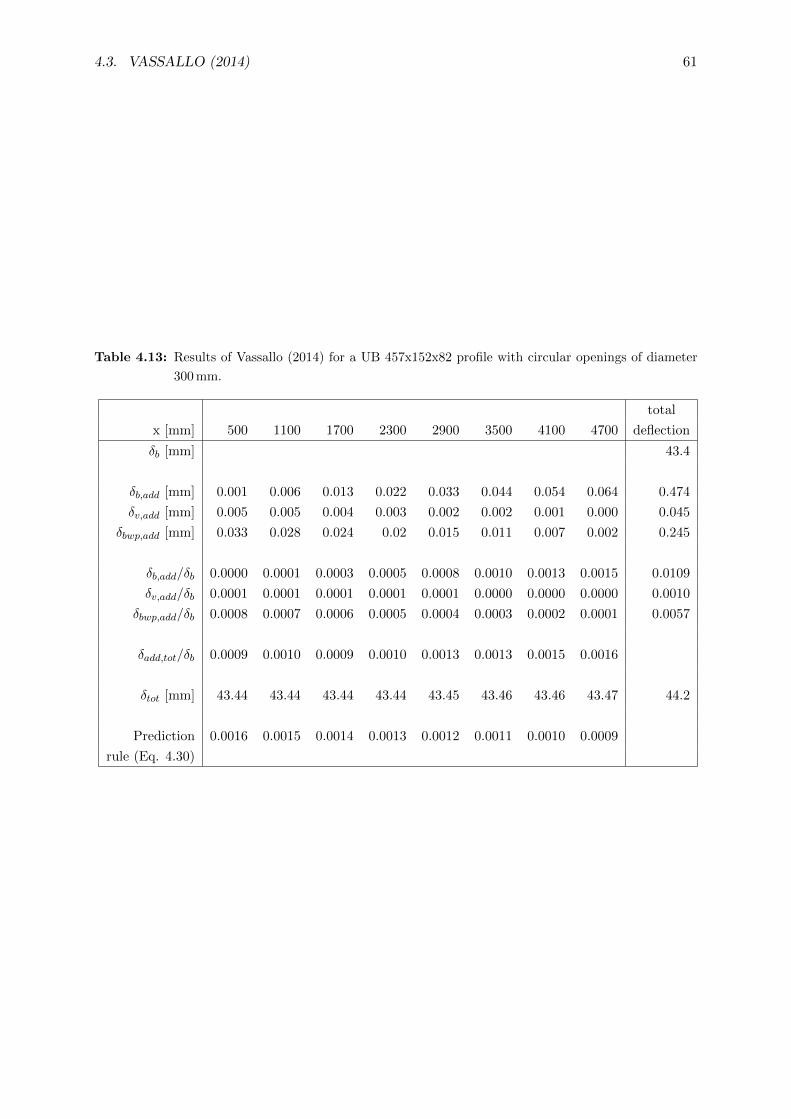
4.3. VASSALLO (2014) 61
Table 4.13: Results of Vassallo (2014) for a UB 457x152x82 profile with circular openings of diameter
300 mm.
total
x [mm] 500 1100 1700 2300 2900 3500 4100 4700 deflection
δb [mm] 43.4
δb,add [mm] 0.001 0.006 0.013 0.022 0.033 0.044 0.054 0.064 0.474
δv,add [mm] 0.005 0.005 0.004 0.003 0.002 0.002 0.001 0.000 0.045
δbwp,add [mm] 0.033 0.028 0.024 0.02 0.015 0.011 0.007 0.002 0.245
δb,add/δb 0.0000 0.0001 0.0003 0.0005 0.0008 0.0010 0.0013 0.0015 0.0109
δv,add/δb 0.0001 0.0001 0.0001 0.0001 0.0001 0.0000 0.0000 0.0000 0.0010
δbwp,add/δb 0.0008 0.0007 0.0006 0.0005 0.0004 0.0003 0.0002 0.0001 0.0057
δadd,tot/δb 0.0009 0.0010 0.0009 0.0010 0.0013 0.0013 0.0015 0.0016
δtot [mm] 43.44 43.44 43.44 43.44 43.45 43.46 43.46 43.47 44.2
Prediction 0.0016 0.0015 0.0014 0.0013 0.0012 0.0011 0.0010 0.0009
rule (Eq. 4.30)
62 CHAPTER 4. ADDITIONAL DEFLECTION

Part II
Numerical investigation
63


Chapter 5
The numerical model
The scope of this thesis is to extend the knowledge obtained in the PhD thesis of Sonck (2014),
that covered the weak-axis flexural buckling and lateral-torsional buckling of cellular and castel-
lated members, with the strong-axis flexural buckling behaviour of castellated and cellular mem-
bers. As such, the same numerical model will be used but with additional boundary conditions,
to obtain strong-axis flexural buckling instead of weak-axis flexural buckling. This chapter,
apart from section 5.3, is thus a summary of the chapter ’Numerical model’ found in Sonck
(2014). All numerical simulations were executed in Abaqus (Dassault Systemes, 2014).
Sonck (2014) states that the numerical model and the used imperfections are based on the
’model column’ approach used for the determination of the column buckling curves. It was
chosen to match the mean minus twice the standard deviation (m-2s) value of the experimental
results as closely as possible (cf. section 3.3.1). Hence, the executed study will be more of a
deterministic nature than of a probabilistic nature.
5.1 Element type and mesh
Shell elements are used to model the flanges and the web of the members in Abaqus. This
corresponds to the wire model approach (cf. section 3.1) that was used to determine the cross-
sectional properties. A consequence of this approach is that the fillets between the web and the
flanges are not taken into account. However, this is partially compensated as there is an overlap
of material at the intersection of the web with the flanges due to the modelling (Fig. 5.1). For
the determination of the buckling curves the dimensionless parameters λ and χ are used. It was
stated by Taras (2010) that there is little difference between the buckling curves determined
based on a model with or without fillets in this format (cf. section 3.1).
For the shell elements the shell type ’S8R’ (quadratic shell element with reduced integration)
was selected, as hourglassing was observed for the reduced first order shell elements (’S4R’ and
’S4R5’) and because the calculations lasted longer with the ’S4’ element (a linear, quadrilateral
fully integrated shell element (Dassault Systemes, 2014)). (Sonck, 2014)
The size of the mesh is determined based on five conditions: there should at least be two
elements along the width of the web post; six elements along the flange width; two elements in
the web of the tee, six elements along the length of an opening and a minimum dimension of
0.03 m should be respected. For cellular members, the size of the mesh is defined for the entire
65
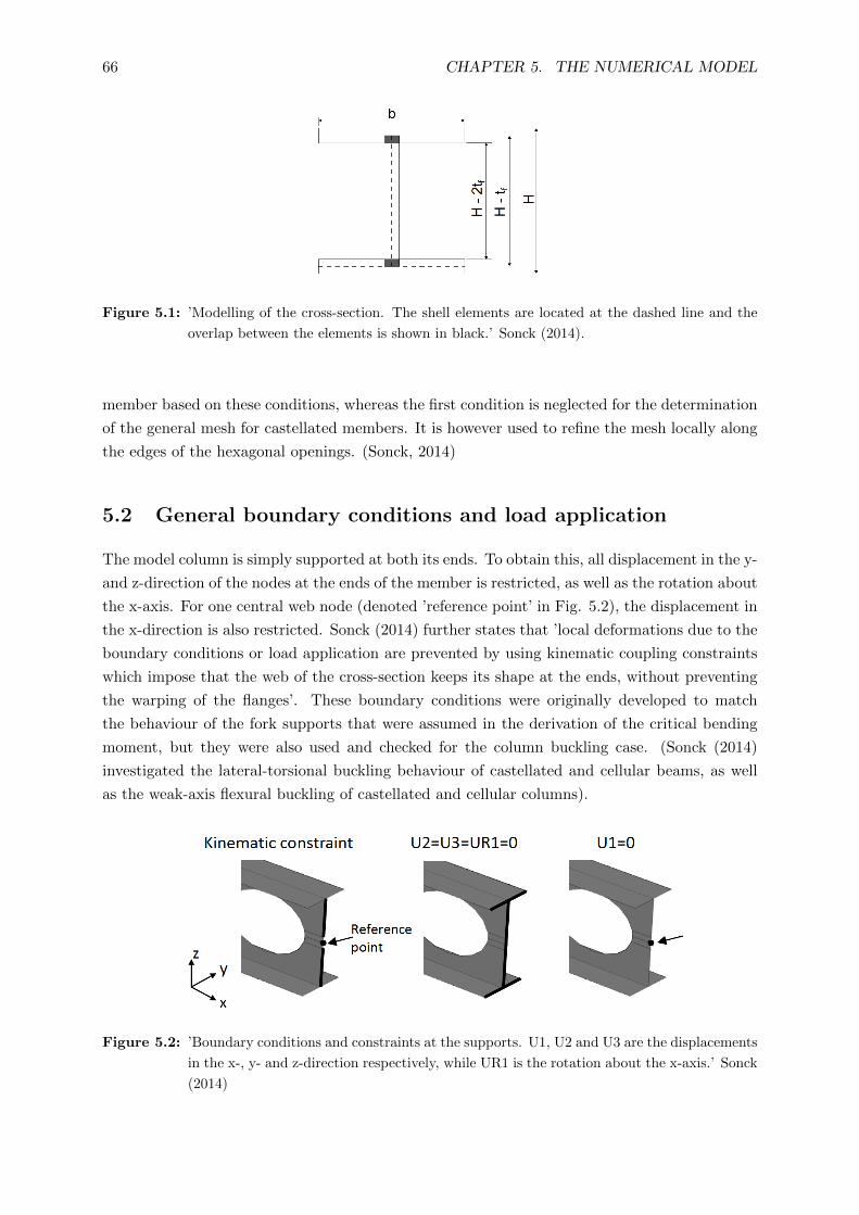
66 CHAPTER 5. THE NUMERICAL MODEL
Figure 5.1: ’Modelling of the cross-section. The shell elements are located at the dashed line and the
overlap between the elements is shown in black.’ Sonck (2014).
member based on these conditions, whereas the first condition is neglected for the determination
of the general mesh for castellated members. It is however used to refine the mesh locally along
the edges of the hexagonal openings. (Sonck, 2014)
5.2 General boundary conditions and load application
The model column is simply supported at both its ends. To obtain this, all displacement in the y-
and z-direction of the nodes at the ends of the member is restricted, as well as the rotation about
the x-axis. For one central web node (denoted ’reference point’ in Fig. 5.2), the displacement in
the x-direction is also restricted. Sonck (2014) further states that ’local deformations due to the
boundary conditions or load application are prevented by using kinematic coupling constraints
which impose that the web of the cross-section keeps its shape at the ends, without preventing
the warping of the flanges’. These boundary conditions were originally developed to match
the behaviour of the fork supports that were assumed in the derivation of the critical bending
moment, but they were also used and checked for the column buckling case. (Sonck (2014)
investigated the lateral-torsional buckling behaviour of castellated and cellular beams, as well
as the weak-axis flexural buckling of castellated and cellular columns).
Figure 5.2: ’Boundary conditions and constraints at the supports. U1, U2 and U3 are the displacements
in the x-, y- and z-direction respectively, while UR1 is the rotation about the x-axis.’ Sonck
(2014)

5.3. ADDITIONAL BOUNDARY CONDITIONS FOR STRONG-AXIS FLEXURAL BUCKLING67
The compressive force N is introduced at the ends of the member in the form of line loads
on both the flanges and the web (Eq. 5.1), corresponding to a single rectangular stress diagram.
σN =N
Aweb + 2 ·Aflange⇒ pflange = σN · tf
pweb = σN · tw (5.1)
5.3 Additional boundary conditions for strong-axis flexural buck-
ling
A column subjected to a normal compressive force will buckle about its weak axis. As this thesis
investigates the strong-axis flexural buckling, boundary conditions have to be added to prevent
weak-axis buckling. Several possibilities were investigated. For each, the critical buckling load
obtained in Abaqus was compared to Ncr,y determined with Eq. 5.2 for plain-webbed members.
In Sweedan et al. (2009), all deformation of the web of the profile is prevented in the Z-direction,
as well as all rotation about the x-axis and the y-axis. Yet, it should be noted that in this article
the column is represented by half the web and half of the flanges, so that these boundary
conditions are strictly necessary to simulate the real behaviour of the column.
The first considered boundary condition consisted of a restriction of the deformation in the
y-direction, as well as a restriction of the rotation about the x-axis and the z-axis. This boundary
condition is applied at the tips of the flanges, and was checked initially for a HE320A plain-
webbed profile. The strong-axis flexural buckling shape was obtained, but from a comparison
between the eigenvalue obtained in Abaqus and the eigenvalue determined with Eq. 5.2 it could
be concluded that too many degrees of freedom were obstructed by these boundary conditions.
The eigenvalue obtained in Abaqus equals 1541.9 kN and the eigenvalue calculated with Eq.
5.2 equals 1425.7 kN, resulting in a difference of 7.5%. This is deemed too large, so that this
boundary condition is discarded.
Ncr,y =π2EIyL2cr
(5.2)
The second considered boundary condition consisted of a restriction of the deformation in
the y-direction, and is applied at the intersection of the web and the flanges. It was evaluated
for the six parent sections mentioned in section 6.1.1 and for six sections with an increased
height equal to 1.5 the height h of the parent sections (see Table 5.1). This was done to be able
to anticipate the behaviour of the cellular and castellated members that also have an increased
height compared to their parent sections. For most of the sections the strong-axis flexural
buckling shape was obtained, yet the web of IPE600 c2, HE650A c2 and HE650M c2 buckled,
as can be seen in Fig. 5.3.
The third considered boundary condition consisted of a restriction of the deformation in
the y-direction, and is applied at the middle of the web. However, almost all sections rotated
about this boundary condition (see Fig. 5.4), expect for IPE300 c1, HE320A c1, HE320M c1
and HE320M c2 who did obtain the strong-axis buckling shape.
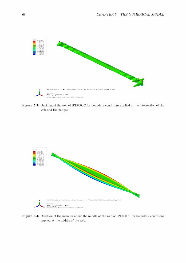
68 CHAPTER 5. THE NUMERICAL MODEL
Figure 5.3: Buckling of the web of IPE600 c2 for boundary conditions applied at the intersection of the
web and the flanges.
Figure 5.4: Rotation of the member about the middle of the web of IPE600 c1 for boundary conditions
applied at the middle of the web.
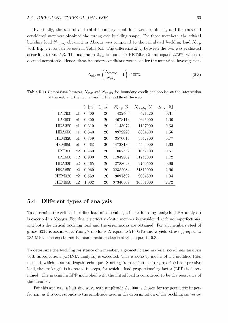
5.4. DIFFERENT TYPES OF ANALYSIS 69
Eventually, the second and third boundary conditions were combined, and for those all
considered members obtained the strong-axis buckling shape. For those members, the critical
buckling load Ncr,abq obtained in Abaqus was compared to the calculated buckling load Ncr,y
with Eq. 5.2, as can be seen in Table 5.1. The difference ∆abq between the two was evaluated
according to Eq. 5.3. The maximum ∆abq is found for HE650M c2 and equals 2.72%, which is
deemed acceptable. Hence, these boundary conditions were used for the numerical investigation.
∆abq =
(Ncr,abq
Ncr,y− 1
)· 100% (5.3)
Table 5.1: Comparison between Ncr,y and Ncr,abq for boundary conditions applied at the intersection
of the web and the flanges and in the middle of the web.
h [m] L [m] Ncr,y [N] Ncr,abq [N] ∆abq [%]
IPE300 c1 0.300 20 422406 421120 0.31
IPE600 c1 0.600 20 4673113 4626900 1.00
HEA320 c1 0.310 20 1145072 1137900 0.63
HEA650 c1 0.640 20 8972220 8834500 1.56
HEM320 c1 0.359 20 3570016 3542800 0.77
HEM650 c1 0.668 20 14728139 14494000 1.62
IPE300 c2 0.450 20 1062532 1057100 0.51
IPE600 c2 0.900 20 11949807 11748000 1.72
HEA320 c2 0.465 20 2788028 2760600 0.99
HEA650 c2 0.960 20 22382684 21816000 2.60
HEM320 c2 0.539 20 9097892 9004300 1.04
HEM650 c2 1.002 20 37340509 36351000 2.72
5.4 Different types of analysis
To determine the critical buckling load of a member, a linear buckling analysis (LBA analysis)
is executed in Abaqus. For this, a perfectly elastic member is considered with no imperfections,
and both the critical buckling load and the eigenmodes are obtained. For all members steel of
grade S235 is assumed, a Young’s modulus E equal to 210 GPa and a yield stress fy equal to
235 MPa. The considered Poisson’s ratio of elastic steel is equal to 0.3.
To determine the buckling resistance of a member, a geometric and material non-linear analysis
with imperfections (GMNIA analysis) is executed. This is done by means of the modified Riks
method, which is an arc length technique. Starting from an initial user-prescribed compressive
load, the arc length is increased in steps, for which a load proportionality factor (LPF) is deter-
mined. The maximum LPF multiplied with the initial load is considered to be the resistance of
the member.
For this analysis, a half sine wave with amplitude L/1000 is chosen for the geometric imper-
fection, as this corresponds to the amplitude used in the determination of the buckling curves by
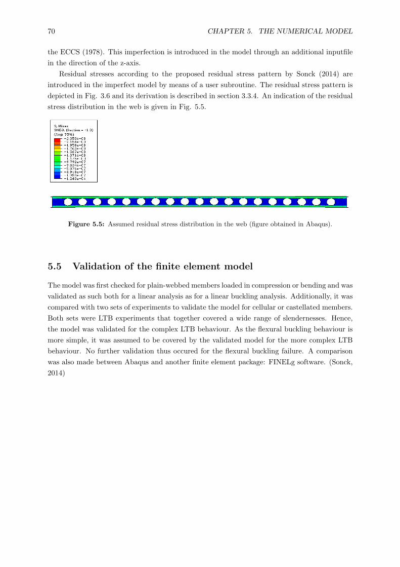
70 CHAPTER 5. THE NUMERICAL MODEL
the ECCS (1978). This imperfection is introduced in the model through an additional inputfile
in the direction of the z-axis.
Residual stresses according to the proposed residual stress pattern by Sonck (2014) are
introduced in the imperfect model by means of a user subroutine. The residual stress pattern is
depicted in Fig. 3.6 and its derivation is described in section 3.3.4. An indication of the residual
stress distribution in the web is given in Fig. 5.5.
Figure 5.5: Assumed residual stress distribution in the web (figure obtained in Abaqus).
5.5 Validation of the finite element model
The model was first checked for plain-webbed members loaded in compression or bending and was
validated as such both for a linear analysis as for a linear buckling analysis. Additionally, it was
compared with two sets of experiments to validate the model for cellular or castellated members.
Both sets were LTB experiments that together covered a wide range of slendernesses. Hence,
the model was validated for the complex LTB behaviour. As the flexural buckling behaviour is
more simple, it was assumed to be covered by the validated model for the more complex LTB
behaviour. No further validation thus occured for the flexural buckling failure. A comparison
was also made between Abaqus and another finite element package: FINELg software. (Sonck,
2014)

Chapter 6
Strong-axis flexural buckling:
parametric study
6.1 Studied parameters
For the investigation of the flexural buckling behaviour about the strong axis of cellular and
castellated columns, several parameters were varied. Six different parent sections were consid-
ered, for which the geometry of the circular and hexagonal openings was varied. Also the length
of the members was varied, to obtain different values for the slenderness λ. The flexural buck-
ling behaviour for these members was determined by running numerical analyses of the members
subjected to a normal force to simulate them as columns loaded in compression.
As the scope of this thesis is to extend the knowledge obtained in the Phd thesis of Sonck
(2014) with the strong-axis flexural buckling behaviour of castellated and cellular members, the
same parameters (parent sections, geometry and slenderness λ) are withheld.
6.1.1 Parent sections
Six European parent sections were selected from the available parent sections in the ArcelorMit-
tal sales catalogue (ArcelorMittal (2008c)) as can be seen in Table 6.1. As these are available
in this sales catalogue, it can be assumed that they are regularly used sections. The IPE300
and IPE600 cover the normal application area, and of the wide flange sections, HEA and HEM
are selected to have the largest possible variation of section properties. To obtain a web height
hweb = h − 2tf that is as similar as possible for all the parent sections, HE320A, HE650A,
HE320M and HE650M are selected. The extra wide flange sections HL and the wide flange
columns HD were not considered, as it is not certain that the proposed residual stress pattern
is also valid for these heavier sections. Including these sections in the investigation would also
complicate a comparison between the different sections. As cited in Sonck (2014), the compres-
sive residual stress magnitude will be larger for the HE320A and the HE320M sections than for
the other sections due to the h/b ratio (see Fig. 3.6).
71

72 CHAPTER 6. STRONG-AXIS FLEXURAL BUCKLING: PARAMETRIC STUDY
Table 6.1: Dimensions of the considered parent sections.
Section h b tw tf
name [mm] [mm] [mm] [mm]
IPE300 300 150 7.1 10.7
IPE600 600 220 12.0 19.0
HE320A 310 300 9.0 15.5
HE650A 640 300 13.5 26.0
HE320M 359 309 21.0 40.0
HE650M 668 305 21.0 40.0
6.1.2 Geometry of the openings
The geometry of the circular and hexagonal openings is described by the dimensions indicated
in section 2.3 and depicted in Fig. 6.1. By varying these parameters, which will be described
below, as well as the length of the members, a large set of different cellular and castellated
member geometries is obtained. The width of the end web posts wend for all the members is
equal to twice the width of the web post w. All the considered geometries are constructed from
one parent section and thus doubly symmetric.
In Appendix C, Tables C.1 and C.2 give a summary of the extreme heights H and openings
heights a of the different geometries. For the cellular columns, nine different sets of geometries
will be considered and for the castellated columns 27 sets of geometries.
Figure 6.1: Indication of the main parameters of cellular and castellated members (extracted from Sonck
(2014)).
Circular openings
Two independent factors determine the geometry of the cellular member openings: fa and fw.
fa determines the height of the opening a, which is function of the height of the original parent

6.1. STUDIED PARAMETERS 73
section (Eq. 6.1). fw determines the width of the web post w, which is function of the width of
the opening `0 (Eq. 6.2).
a = fa ·h (6.1)
w = fw · `0 = fw · a (6.2)
In ArcelorMittal (2008c) and in ArcelorMittal (2008a), the range of often used values for
these factors is found. Based on these, as well as on the geometric constraints cited in section 2.4,
three values are withheld for fa and fw (Table 6.2). With these values a and w are determined,
and thus also H with Eq. 2.1. A set of 9 different geometries is obtained in this way, and for
each set it is checked whether all geometric constraints cited in section 2.4 are fulfilled. In case
they are not, the set is not considered for the parametric study. An overview of these can be
found in Appendix B in Table B.3.
Table 6.2: Considered values for fa and fw.
factor considered values
fa 0.8 1.0 1.2
fw 0.1 0.4 0.7
Hexagonal openings
The geometry of castellated members is defined by three independent factors: fH , α and fw.
fH determines the increased height H of the member according to Eq. 6.3, which is also used
to determine the height of the opening a. The angle of the opening α defines c (Eq. 6.4) and
fw determines the width of the web post w (Eq. 6.5). The length of the hexagonal opening `0
is determined by c and w, as illustrated in Eq. 6.5.
H = fHh = h+a
2(6.3)
c =a
2tan(α)(6.4)
w = fwl0 = fw(w + 2c) (6.5)
Table 6.3 gives the chosen values for these three factors. The values for fH were determined
based on the general range of H/h. The opening angle α is varied to obtain Angelina like web
openings (α = 45◦), regular hexagonal web openings (α = 60◦) and nearly diamond shaped web
openings (α = 75◦). For fw similar values are chosen as for the cellular members. However, they
are slightly smaller in order to meet the geometric constraints listed in section 2.4. Furthermore,
they are based on the values for the two standard castellated beam geometries that are mentioned
in section 2.3.
The considered values in Table 6.3 define 27 different sets of geometries, for which the
geometric constraints mentioned in section 2.4 are checked. Those sets of geometries that do
not fulfil these constraints are not considered in the parametric study; they can be found in
Appendix B in Tables B.1 and B.2.

74 CHAPTER 6. STRONG-AXIS FLEXURAL BUCKLING: PARAMETRIC STUDY
Table 6.3: Considered values for fH , α and fw.
factor considered values
fH 1.4 1.5 1.6
α 45◦ 60◦ 75◦
fw 0.1 0.3 0.5
An illustration of some geometries is found in Fig. 6.2.
Figure 6.2: Illustration of some geometries for cellular and castellated members.
6.1.3 Length of the member
The length of a castellated member is found using Eq. 6.6, the length of a cellular member is
found with Eq. 6.7. Hence, the length is mainly determined by the number of openings n in
the member. This number n is chosen in such a way that the slenderness λ for a given set of
geometries (e.g. fa=0.8 and fw=0.4 for a cellular member) varies around 0.5, 1.0, 1.5, 2.0 or
2.5. This way five different lengths (and slenderness) are obtained for a given set of geometries.
It is also ensured that the length of a member is at least equal to five times its height H.
For cellular members nine different sets of geometries were obtained, and for each of these sets
five different member lengths (and slenderness λ) are considered. As such, there are 45 different
members considered for each parent section, leading to a total of 270 considered members of the
cellular type. For castellated members 27 sets of geometries were defined, which were considered
for five different member lengths. There was a total of 135 members for each parent section, so
that 810 different members of the castellated type were considered in total.
L = 2 ·wend + n · (w + 2c) + (n− 1) ·w (6.6)
L = (n− 1) ·w + n · a+ 2 ·wend (6.7)
This range for the slenderness λ corresponds to the range of λ that is used to present the
flexural buckling curves (see Fig. 3.4). However, for strong-axis flexural buckling this range

6.1. STUDIED PARAMETERS 75
leads to maximal member lengths of approximately 120 m for the larger parent sections and
approximately 60 m for the smaller parent sections (Table 6.4). Such a height for a column is
highly unrealistic. Yet, these lengths are still considered in order to propose a buckling curve
whereby the total range of slenderness λ is taken into account.
Table 6.4: Extreme values of the considered lengths for the different parent sections.
Castellated members Cellular members
min L [m] max L [m] min L [m] max L [m]
IPE300 9.022 54.687 8.256 53.568
IPE600 18.044 109.373 16.512 107.136
HE320A 9.323 56.510 8.531 55.354
HE650A 19.247 116.665 17.613 114.278
HE320M 10.796 65.442 9.880 59.343
HE650M 20.089 121.769 18.383 119.278
6.1.4 Load case and boundary conditions
The members are subjected to a constant normal compressive force N, and are simply supported.
To prevent weak-axis flexural buckling, additional boundary conditions are added to the model:
the deformation in the y-direction is obstructed at the intersection of the web with the flanges
and in the middle of the web. How these boundary conditions were obtained is discussed in
section 5.3. Sonck (2014) states that for weak-axis flexural buckling the modified geometry
(the height of the cellular or castellated member has increased compared to the height of its
parent section) will have a smaller effect than for strong-axis buckling. However, the influence
of the modified residual stress pattern proposed by Sonck (2014) (section 3.3.4) will be larger
for weak-axis bucking than for strong-axis buckling.
6.1.5 Determination of the class of the cross-section
The classification of the cross section is determined as described in section 3.3.2. The classifi-
cation check is executed for the flanges, the web at the web post section and the web at the tee
section. For the cross-section as a whole, the most detrimental classification of these three parts
is withheld. The results of these checks can be found in Appendix C in Tables C.1 and C.2.
The flanges are class 1 for all considered geometries. At the openings, the tee sections are
class 2. At the location of the web posts however, the most detrimental classification is class 4,
except for the geometries derived from the parent section HE320M (class 1). This is due to the
enlarged height of the web at the web post. Hence, cross-section class 4 is adopted, which implies
that a central opening should be introduced in the web to obtain an effective cross-section Aeff .
The height of this opening is equal to aeff , for which the specific values can also be found in
Tables C.1 and C.2.
In these tables the minimum and maximum values of the opening height a can also be found.
This opening height was used to calculate the plastic properties of the cross-section, and is larger
than aeff for every considered geometry. Hence, the plastic resistance of the cross-section at the
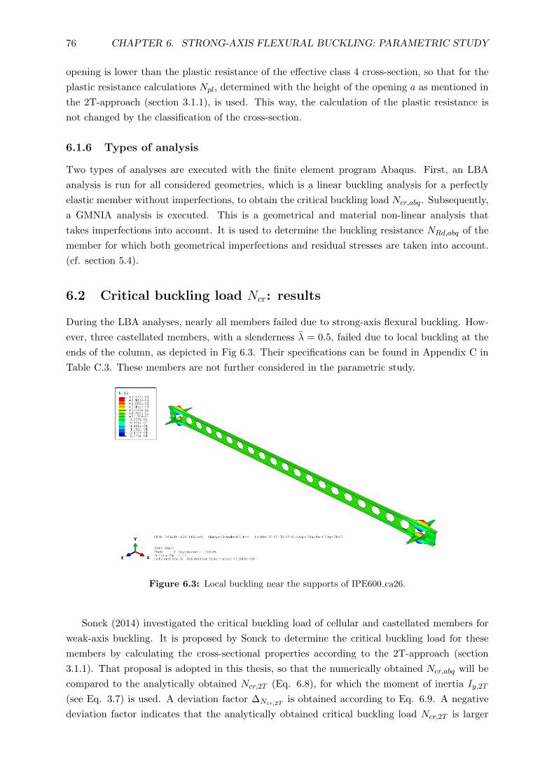
76 CHAPTER 6. STRONG-AXIS FLEXURAL BUCKLING: PARAMETRIC STUDY
opening is lower than the plastic resistance of the effective class 4 cross-section, so that for the
plastic resistance calculations Npl, determined with the height of the opening a as mentioned in
the 2T-approach (section 3.1.1), is used. This way, the calculation of the plastic resistance is
not changed by the classification of the cross-section.
6.1.6 Types of analysis
Two types of analyses are executed with the finite element program Abaqus. First, an LBA
analysis is run for all considered geometries, which is a linear buckling analysis for a perfectly
elastic member without imperfections, to obtain the critical buckling load Ncr,abq. Subsequently,
a GMNIA analysis is executed. This is a geometrical and material non-linear analysis that
takes imperfections into account. It is used to determine the buckling resistance NRd,abq of the
member for which both geometrical imperfections and residual stresses are taken into account.
(cf. section 5.4).
6.2 Critical buckling load Ncr: results
During the LBA analyses, nearly all members failed due to strong-axis flexural buckling. How-
ever, three castellated members, with a slenderness λ = 0.5, failed due to local buckling at the
ends of the column, as depicted in Fig 6.3. Their specifications can be found in Appendix C in
Table C.3. These members are not further considered in the parametric study.
Figure 6.3: Local buckling near the supports of IPE600 ca26.
Sonck (2014) investigated the critical buckling load of cellular and castellated members for
weak-axis buckling. It is proposed by Sonck to determine the critical buckling load for these
members by calculating the cross-sectional properties according to the 2T-approach (section
3.1.1). That proposal is adopted in this thesis, so that the numerically obtained Ncr,abq will be
compared to the analytically obtained Ncr,2T (Eq. 6.8), for which the moment of inertia Iy,2T
(see Eq. 3.7) is used. A deviation factor ∆Ncr,2Tis obtained according to Eq. 6.9. A negative
deviation factor indicates that the analytically obtained critical buckling load Ncr,2T is larger

6.2. CRITICAL BUCKLING LOAD NCR: RESULTS 77
than the numerically obtained Ncr,abq, which is unsafe. A positive deviation factor indicates the
opposite.
However, it should be emphasized that an additional reduction factor will be necessary. In
sections 3.4, 3.5 and 4 it was already stated that the reduced shear stiffness of the cross-section
due to the presence of the openings will decrease the strong-axis critical buckling load Ncr due
to increased shear deformations. In the 2T-approach, it is proposed to determine the cross-
sectional properties in the middle of an opening, so that only the bending stiffness of the two
tee sections is taken into account. In this approach, it is assumed that the shear deformation is
equal to zero, which is certainly not the case for strong-axis flexural buckling. As such, Ncr,2T
will overestimate the critical buckling load.
For the weak-axis critical buckling load, the shear stiffness has no significant influence. If the
member is compared to a built-up compression member, weak-axis buckling occurs about the
axis crossing the chords (which are the tee sections in case of cellular or castellated members),
the battenings (or web posts) do not play a roll. Hence, half of the compressive force is taken
by each tee section, so that the weak-axis critical buckling load can be accurately determined
by replacing Iz by Iz,2T (Sonck, 2014). Additionally, the difference between Iz,2T and Iz is not
that large because the contribution of the web, in which the opening is located, to the weak-axis
bending stiffness is rather small.
Ncr,2T =π2EIy,2T
l2cr(6.8)
∆Ncr,2T=
(Ncr,abq
Ncr,2T− 1
)· 100% (6.9)
The need for a reduction factor is apparent from figures 6.4 and 6.5, that display the deviation
factor for the cellular columns and the castellated columns respectively. For castellated columns,
the deviation is limited to ±5% for members longer than 25 m, or with a slenderness λ exceeding
1. However, the realistic lengths for columns are below this value, and thus for slendernesses
smaller than 1, and for those a reduction factor is necessary. The largest deviation is found
for the HE320A parent section. The flanges for a HE320A section are wide (b=h) compared
to the height of the section, so that the ratio Af/Aw, which stands for the area of one flange
divided by the area of the web, is equal to 2. Hence, there is much more flange present, leading
to higher shear deformations in the web. For the IPE300 parent section Af/Aw equals 0.75,
and it is apparent that for this parent section the required reduction factor is less. Hence, it
might be concluded that the ratio Af/Aw has an important influence on the required reduction
factor. This ratio depends on the parent section, and is thus not influenced by the geometry of
openings. However, there is still a large variation for the deviation of each parent section, so
that is excepted that the geometry of the openings will also have an influence.
In Appendix C, the results of a comparison between Ncr,abq and Ncr,0 are also given. Ncr,0 is
the critical buckling load determined for the full cross section, which is only present at the web
post sections. For weak-axis flexural buckling, the presence of the opening has little influence
as Iz,0 differs only slightly from Iz,2T , so that the difference between Ncr,0 and Ncr,2T is small
(Sonck, 2014). On the other hand, for strong-axis flexural buckling, the presence of the openings
significantly influence the moment of inertia Iy (Iy,2T is significantly smaller than Iy,0), so that

78 CHAPTER 6. STRONG-AXIS FLEXURAL BUCKLING: PARAMETRIC STUDY
0 20 40 60 80 100 120
Length [m]
−30
−25
−20
−15
−10
−5
0
5
∆Ncr,
2T
=Ncr,abq/N
cr,2T−
1[%
]
Cellular columns
IPE300IPE600HE320AHE650AHE320MHE650M
Figure 6.4: Deviation between Ncr,abq and Ncr,2T for cellular columns.
0 20 40 60 80 100 120
Length [m]
−30
−25
−20
−15
−10
−5
0
5
∆Ncr,
2T
=Ncr,abq/N
cr,2T−
1[%
]
Castellated columns
IPE300IPE600HE320AHE650AHE320MHE650M
Figure 6.5: Deviation between Ncr,abq and Ncr,2T for castellated columns.

6.2. CRITICAL BUCKLING LOAD NCR: RESULTS 79
there is a significant difference between Ncr,0 and Ncr,2T . Consequently, using Ncr,0 to predict
the actual strong-axis critical buckling load would be even more unsafe than using Ncr,2T .
6.2.1 Comparison between Ncr,abq and Ncr obtained for a battened compres-
sion column
In section 3.4, the equations are given to be able to calculate the strong-axis critical buckling
load for battened compression columns, adapted to be applicable for cellular and castellated
columns. It is pointed out in that section that cellular and castellated columns can be seen as
battened compression columns, whereby the tee sections are considered to be the chords and
the web posts considered to be the battenings.
∆Nbattenings=
(Ncr,abq
Ncr,battenings− 1
)· 100% (6.10)
In Fig. 6.6 and Fig. 6.7, the deviation factor ∆Nbattenings(Eq. 6.10), is given for cellular and
castellated columns. The deviation factor is mainly positive, which indicates that the critical
buckling load Ncr,battenings determined with Eq. 3.23 results in a lower value than the critical
buckling load Ncr,abq that is obtained in Abaqus, which is considered safe. However, the critical
buckling load Ncr is severly underestimated for the shortest members, with deviations up to
120% for the castellated columns and 85% for the cellular columns. These extreme values
arise for those geometries that result in large widths of the web post (fa=1.0 and fw=0.7;
fa=1.2 and fw=0.4) for the cellular geometries. For the castellated members (see Table 6.5),
they arise for large widths of the web post combined with a lower opening angle α for the
castellated opening, as this results in a larger web post (fH=1.6 and α=60◦and fw=0.5, fH=1.6
and α=45◦and fw=0.3). In the derivation of Ncr,battenings (Eq. 3.23), the battenings and the
chords are modelled as lines, and it is assumed that the battenings have a limited cross-section.
Additionally, the battenings are considered to be bolted to the chords. The geometries with
the widest web posts do not confirm to those assumptions, hence the large deviations for those
geometries. This was also stated by Sweedan et al. (2009). The width of the web post should
be taken into account in the derivation of ∆Nbatteningsto obtain a better result. It can thus be
concluded that Eq. 3.23 should not be used to predict the major-axis critical buckling load, as
it leads to overly conservative values.
6.2.2 Comparison between Ncr,abq and Ncr obtained with the proposed Ieq in
section 4
In section 4, approximate equations (Eq. 4.9, Eq. 4.11 and Eq. 4.13) to predict the additional
deflection of cellular and castellated beams due to the presence of the openings were examined.
They actually propose an equivalent bending stiffness Ieq (Eq. 4.2) to determine the total
deflection with, in which the effect of the presence of the openings is accounted for. Hence, Ncr
determined with this equivalent bending stiffness might predict the major axis critical buckling
load. The equivalent bending stiffness is different for the castellated members than for the
cellular members: for the castellated members it is determined as in Eq. 6.12, for the cellular
members as in Eq. 6.11. With these Ieq,y,2T Ncr is determined and compared to Ncr,abq in Fig.
6.8 and 6.9.

80 CHAPTER 6. STRONG-AXIS FLEXURAL BUCKLING: PARAMETRIC STUDY
0 20 40 60 80 100 120
Length [m]
−20
0
20
40
60
80
100
120∆Nbattenings
=Ncr,abq/N
cr,battenings−
1[%
]
Cellular columns
IPE300IPE600HE320AHE650AHE320MHE650M
Figure 6.6: Deviation between Ncr,abq and Ncr,battenings for cellular columns.
0 20 40 60 80 100 120
Length [m]
−20
0
20
40
60
80
100
120
∆Nbattenings
=Ncr,abq/N
cr,battenings−
1[%
]
Castellated columns
IPE300IPE600HE320AHE650AHE320MHE650M
Figure 6.7: Deviation between Ncr,abq and Ncr,battenings for castellated columns.

6.2. CRITICAL BUCKLING LOAD NCR: RESULTS 81
Table 6.5: The maximum found ∆Nbatteningsfor the castellated columns (λ = 0.5 for all parent sections).
fH α fw c w Ncr,abq [N] Ncr,battenings [N] ∆Nbattenings
IPE300 1.6 45 0.3 0.180 0.154 3267100 1832909 78.25
IPE300 1.6 60 0.5 0.104 0.208 3460000 2066516 67.43
HE320A 1.6 45 0.3 0.186 0.159 7641700 3464676 120.56
HE320A 1.6 60 0.5 0.107 0.215 7811700 3926145 98.97
IPE600 1.6 45 0.3 0.360 0.309 9187500 5467827 68.03
IPE600 1.6 60 0.5 0.208 0.416 9786600 6154747 59.01
HE650A 1.6 45 0.3 0.384 0.329 15064000 8042204 87.31
HE650A 1.6 60 0.5 0.222 0.443 15845000 9078386 74.54
HE650M 1.6 45 0.3 0.401 0.344 23096000 12235904 88.76
HE650M 1.6 60 0.5 0.231 0.463 24345000 13813148 76.25
Ieq,y,2T,cell =Iy,2T(
1 + 0.7nk00.45a2
LH
) (6.11)
Ieq,y,2T,cast =Iy,2T(
1 + 0.7nk00.5(w+2c)a
LH
) (6.12)
0 20 40 60 80 100 120
Length [m]
0
10
20
30
40
∆Ncr,Ieq
=Ncr,abq/N
cr,Ieq−
1[%
]
Cellular columns
IPE300IPE600HE320AHE650AHE320MHE650M
Figure 6.8: Deviation between Ncr,abq and Ncr,Ieq for cellular columns.
From Fig. 6.8 and 6.9, it is clear that also this proposal for the determination of Ncr is not
satisfactory. Most Ncr,Ieq are smaller than Ncr,abq, and thus safe. However, for larger lengths
(and thus larger slendernesses), deviations up to 35% are obtained for the cellular columns,

82 CHAPTER 6. STRONG-AXIS FLEXURAL BUCKLING: PARAMETRIC STUDY
0 20 40 60 80 100 120
Length [m]
0
10
20
30
40
∆Ncr,Ieq
=Ncr,abq/N
cr,Ieq−
1[%
]
Castellated columns
IPE300IPE600HE320AHE650AHE320MHE650M
Figure 6.9: Deviation between Ncr,abq and Ncr,Ieq for castellated columns.
and up to 40% for the castellated columns. This is a large underestimation of the critical
buckling load. The other two proposals, Ncr,2T determined with the cross-sectional properties
at the middle of the opening and Ncr,battenings determined for the members approximated by a
battened compression column are than more satisfactory, although either an overestimation of
Ncr,abq is obtained or an underestimation for the members with the shortest lengths (which are
also the most realistic members). Further investigation would be necessary to find an appropriate
reduction factor so that Ncr,abq can be accurately predicted.
6.3 Buckling resistance NRd: results
During the GMNIA analyses, most members failed due to strong-axis buckling. In this type of
analysis the load proportionality factor (LPF) is determined, after which it is plotted in function
of the displacement to be able to determine whether a clear maximum is reached. A typical load
proportionality factor - displacement diagram (LPF-U2) is given in Fig. 6.10a for a member
that buckles. The maximum found LPF is used to determine the buckling resistance NRd,abq.
Yet for some members no clear maximum is found on the LPF-U2 diagram, as the diagram
displays a plateau (as in Fig. 6.10b). The maximum LPF obtained for those members is com-
pared to the maximum LPF of members with a similar length that do obtain a clear maximum
in the LPF-U2 diagram. In case the displacement U2 at the maximum LPF is nearly the same,
it is concluded that these members (that show a plateau on their LPF-U2 diagram) also reach
their maximum LPF. However, for some members no such comparison could be made so that it
is uncertain whether these members did reach their maximum LPF. These members are added
to the ’shadow list’ (Appendix C): in case there is uncertainty about the selection of the buckling

6.3. BUCKLING RESISTANCE NRD: RESULTS 83
curve, the results obtained for those members will be left out of the analysis.
(a) IPE300 c16 (L=9.99 m, fa=1.0, fw=0.1) (b) IPE300 c18 (L=29.79 m, fa=1.0, fw=0.1)
Figure 6.10: Diagram of the load proportionality factor versus the displacement along the z-axis during
a GMNIA analysis (obtained with the program Abaqus).
Apart from the members that showed a plateau in their LPF-U2 diagram, some members
failed locally at the end web posts due to plastic failure, as depicted in Fig. 6.11. The plastic
resistance is reached locally at the end web post, after which it folds into itself. Their specifi-
cations can be found in Appendix C in Tables C.4 and C.5 and these members are not further
considered in the study.
However, it is remarkable that these members all have a similar geometry: for the castellated
members α=75◦and fw=0.3 for all these members and for the cellular members fw=0.1 (see
section 6.1.2 for the definition of the factors). These factors lead to a smaller end web post than
for other geometries. As the load is introduced at the end web post, there is thus only little
material available to distribute the stresses further into the member. Furthermore, the stress
concentrations that appear around the edges of the opening are located close by the edge of the
member due to the small end web post, so that the yield stress is sooner reached in this region.
Figure 6.11: Local failure at the end web post of HE320M ca81 (L=29.79 m, fH=1.5, α=75◦and
fw=0.3) (figure obtained with the program Abaqus).
The buckling resistance NRd,abq is obtained from the program Abaqus by multiplying the
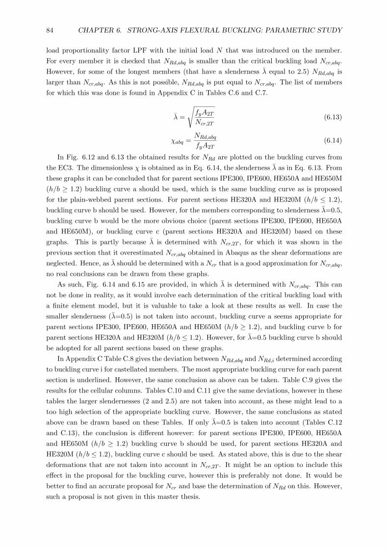
84 CHAPTER 6. STRONG-AXIS FLEXURAL BUCKLING: PARAMETRIC STUDY
load proportionality factor LPF with the initial load N that was introduced on the member.
For every member it is checked that NRd,abq is smaller than the critical buckling load Ncr,abq.
However, for some of the longest members (that have a slenderness λ equal to 2.5) NRd,abq is
larger than Ncr,abq. As this is not possible, NRd,abq is put equal to Ncr,abq. The list of members
for which this was done is found in Appendix C in Tables C.6 and C.7.
λ =
√fyA2T
Ncr,2T(6.13)
χabq =NRd,abq
fyA2T(6.14)
In Fig. 6.12 and 6.13 the obtained results for NRd are plotted on the buckling curves from
the EC3. The dimensionless χ is obtained as in Eq. 6.14, the slenderness λ as in Eq. 6.13. From
these graphs it can be concluded that for parent sections IPE300, IPE600, HE650A and HE650M
(h/b ≥ 1.2) buckling curve a should be used, which is the same buckling curve as is proposed
for the plain-webbed parent sections. For parent sections HE320A and HE320M (h/b ≤ 1.2),
buckling curve b should be used. However, for the members corresponding to slenderness λ=0.5,
buckling curve b would be the more obvious choice (parent sections IPE300, IPE600, HE650A
and HE650M), or buckling curve c (parent sections HE320A and HE320M) based on these
graphs. This is partly because λ is determined with Ncr,2T , for which it was shown in the
previous section that it overestimated Ncr,abq obtained in Abaqus as the shear deformations are
neglected. Hence, as λ should be determined with a Ncr that is a good approximation for Ncr,abq,
no real conclusions can be drawn from these graphs.
As such, Fig. 6.14 and 6.15 are provided, in which λ is determined with Ncr,abq. This can
not be done in reality, as it would involve each determination of the critical buckling load with
a finite element model, but it is valuable to take a look at these results as well. In case the
smaller slenderness (λ=0.5) is not taken into account, buckling curve a seems appropriate for
parent sections IPE300, IPE600, HE650A and HE650M (h/b ≥ 1.2), and buckling curve b for
parent sections HE320A and HE320M (h/b ≤ 1.2). However, for λ=0.5 buckling curve b should
be adopted for all parent sections based on these graphs.
In Appendix C Table C.8 gives the deviation betweenNRd,abq andNRd,i determined according
to buckling curve i for castellated members. The most appropriate buckling curve for each parent
section is underlined. However, the same conclusion as above can be taken. Table C.9 gives the
results for the cellular columns. Tables C.10 and C.11 give the same deviations, however in these
tables the larger slendernesses (2 and 2.5) are not taken into account, as these might lead to a
too high selection of the appropriate buckling curve. However, the same conclusions as stated
above can be drawn based on these Tables. If only λ=0.5 is taken into account (Tables C.12
and C.13), the conclusion is different however: for parent sections IPE300, IPE600, HE650A
and HE650M (h/b ≥ 1.2) buckling curve b should be used, for parent sections HE320A and
HE320M (h/b ≤ 1.2), buckling curve c should be used. As stated above, this is due to the shear
deformations that are not taken into account in Ncr,2T . It might be an option to include this
effect in the proposal for the buckling curve, however this is preferably not done. It would be
better to find an accurate proposal for Ncr and base the determination of NRd on this. However,
such a proposal is not given in this master thesis.

6.3. BUCKLING RESISTANCE NRD: RESULTS 85
0.0 0.5 1.0 1.5 2.0 2.5 3.0
λ [-]
0.0
0.2
0.4
0.6
0.8
1.0
1.2
χ[-
]χel
a
b
c
d
Cellular columns
IPE300IPE600HE320AHE650AHE320MHE650M
Figure 6.12: NRd compared with the buckling curves for cellular columns.
0.0 0.5 1.0 1.5 2.0 2.5 3.0
λ [-]
0.0
0.2
0.4
0.6
0.8
1.0
1.2
χ[-
]
χel
a
b
c
d
Castellated columns
IPE300IPE600HE320AHE650AHE320MHE650M
Figure 6.13: NRd compared with the buckling curves for castellated columns.

86 CHAPTER 6. STRONG-AXIS FLEXURAL BUCKLING: PARAMETRIC STUDY
0.0 0.5 1.0 1.5 2.0 2.5 3.0
λ [-]
0.0
0.2
0.4
0.6
0.8
1.0
1.2
χ[-
]χel
a
b
c
d
Cellular columns
IPE300IPE600HE320AHE650AHE320MHE650M
Figure 6.14: NRd compared with the buckling curves for cellular columns. (λ determined with Ncr,abq).
0.0 0.5 1.0 1.5 2.0 2.5 3.0
λ [-]
0.0
0.2
0.4
0.6
0.8
1.0
1.2
χ[-
]
χel
a
b
c
d
Castellated columns
IPE300IPE600HE320AHE650AHE320MHE650M
Figure 6.15: NRd compared with the buckling curves for cellular columns. (λ determined with Ncr,abq).

Part III
Conclusions
87


Chapter 7
Conclusions
In the introduction the following two objectives are stated:
• How is the critical major axis buckling load influenced by the presence of the openings in
the web?
• How is the major axis buckling resistance influenced by the presence of the openings in
the web, taking both geometrical and material imperfections into account?
Due to the openings in the web, increased shear deformations occur that cause a significant
decrease in the critical major axis buckling load for members with a slenderness λ equal to 0.5
or 1.0. This decrease is larger for parent sections with a high ratio Af/Aw, as the web will
deform more for those members due to the smaller shear stiffness of the web. Also, geometries
that correspond to large openings and small widths of the web post show a larger decrease of
the critical major axis buckling load.
Two proposals for the determination of the major axis critical buckling load were compared
to the Ncr,abq obtained in Abaqus. The idea behind these proposals was that they would include
for the decreased shear stiffness of the castellated and cellular columns. However, neither proved
to be satisfactory, so that further research is advised on a proposal for the determination of an
accurate Ncr for castellated and cellular columns.
As no accurate approximation of Ncr was found, no proposal can be made with respect
to the selection of a buckling curve for the castellated and cellular columns. This is because
the slenderness λ should be expressed in function of Ncr to obtain an accurate proposal for a
buckling curve. However, the results are still studied, both in function of λ found with Ncr,abq
obtained in Abaqus and in function of λ found with Ncr,2T . From this it could be concluded
that buckling curve a is appropriate for parent sections IPE300, IPE600, HE650A and HE650M
(h/b ≥ 1.2), and buckling curve b for parent sections HE320A and HE320M (h/b ≤ 1.2). These
are the same buckling curves as proposed for those parent sections without openings in the web.
However, these buckling curves are selected based on all slendernesses, whereas for a slenderness
λ equal to 0.5, corresponding to realistic lengths of columns, a lower buckling curve is more
appropriate. For columns corresponding to this slenderness, buckling curve b is appropriate for
parent sections IPE300, IPE600, HE650A and HE650M (h/b ≥ 1.2), and buckling curve c for
parent sections HE320A and HE320M (h/b ≤ 1.2). This implies that for slendernesses exceeding
1.0, the presence of the openings has negligible influence on the buckling resistance.
89

90 CHAPTER 7. CONCLUSIONS

Part IV
Appendices
91

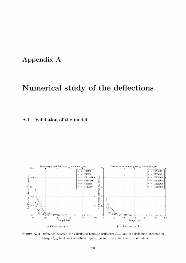
Appendix A
Numerical study of the deflections
A.1 Validation of the model
0 20 40 60 80 100Length [m]
0
10
20
30
40
50
%di
ffer
ence
betw
eenδ abq
andδ calc
Geometry 2 (cellular type): fa = 0.8 and fw=0.7
IPE300IPE600HE320MHE650MHE320AHE650A
(a) Geometry 2.
0 20 40 60 80 100 120Length [m]
0
10
20
30
40
50
%di
ffer
ence
betw
eenδ abq
andδ calc
Geometry 3 (cellular type): fa = 1.0 and fw=0.7
IPE300IPE600HE320MHE650MHE320AHE650A
(b) Geometry 3.
Figure A.1: Difference between the calculated bending deflection δcalc and the deflection obtained in
Abaqus δabq in % for the cellular type subjected to a point load in the middle.
93
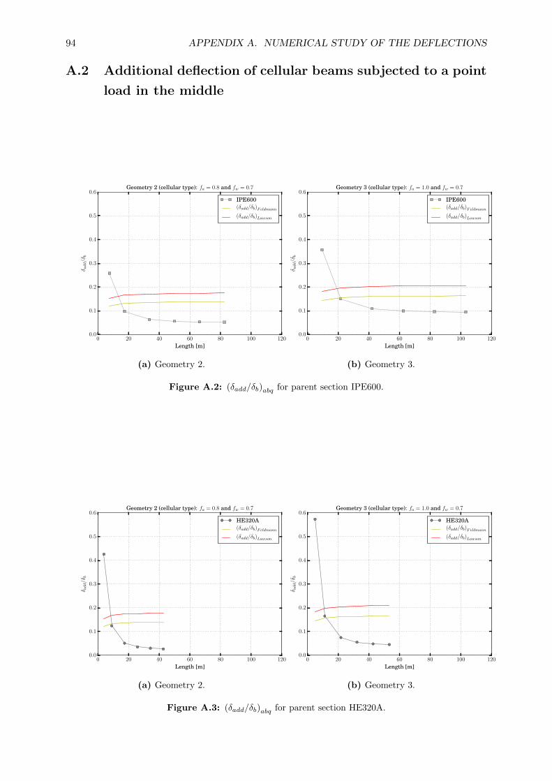
94 APPENDIX A. NUMERICAL STUDY OF THE DEFLECTIONS
A.2 Additional deflection of cellular beams subjected to a point
load in the middle
0 20 40 60 80 100 120
Length [m]
0.0
0.1
0.2
0.3
0.4
0.5
0.6
δ add/δb
Geometry 2 (cellular type): fa = 0.8 and fw = 0.7
IPE600(δadd/δb)Feldmann
(δadd/δb)Lawson
(a) Geometry 2.
0 20 40 60 80 100 120
Length [m]
0.0
0.1
0.2
0.3
0.4
0.5
0.6
δ add/δb
Geometry 3 (cellular type): fa = 1.0 and fw = 0.7
IPE600(δadd/δb)Feldmann
(δadd/δb)Lawson
(b) Geometry 3.
Figure A.2: (δadd/δb)abq for parent section IPE600.
0 20 40 60 80 100 120
Length [m]
0.0
0.1
0.2
0.3
0.4
0.5
0.6
δ add/δb
Geometry 2 (cellular type): fa = 0.8 and fw = 0.7
HE320A(δadd/δb)Feldmann
(δadd/δb)Lawson
(a) Geometry 2.
0 20 40 60 80 100 120
Length [m]
0.0
0.1
0.2
0.3
0.4
0.5
0.6
δ add/δb
Geometry 3 (cellular type): fa = 1.0 and fw = 0.7
HE320A(δadd/δb)Feldmann
(δadd/δb)Lawson
(b) Geometry 3.
Figure A.3: (δadd/δb)abq for parent section HE320A.

A.2. ADDITIONAL DEFLECTIONOF CELLULAR BEAMS SUBJECTED TOA POINT LOAD IN THEMIDDLE95
0 20 40 60 80 100 120
Length [m]
0.0
0.1
0.2
0.3
0.4
0.5
0.6δ add/δb
Geometry 2 (cellular type): fa = 0.8 and fw = 0.7
HE650A(δadd/δb)Feldmann
(δadd/δb)Lawson
(a) Geometry 2.
0 20 40 60 80 100 120
Length [m]
0.0
0.1
0.2
0.3
0.4
0.5
0.6
δ add/δb
Geometry 3 (cellular type): fa = 1.0 and fw = 0.7
HE650A(δadd/δb)Feldmann
(δadd/δb)Lawson
(b) Geometry 3.
Figure A.4: (δadd/δb)abq for parent section HE650A.
0 20 40 60 80 100 120
Length [m]
0
1
2
3
4
5
δ add/δb
Geometry 1 (cellular type): fa = 1.3 and fw = 0.1
HE320A(δadd/δb)Feldmann
(δadd/δb)Lawson
(a) parent section HE320A.
0 20 40 60 80 100 120
Length [m]
0
1
2
3
4
5
δ add/δb
Geometry 1 (cellular type): fa = 1.3 and fw = 0.1
HE320M(δadd/δb)Feldmann
(δadd/δb)Lawson
(b) parent section HE320M.
Figure A.5: (δadd/δb)abq for geometry 1.

96 APPENDIX A. NUMERICAL STUDY OF THE DEFLECTIONS
0 20 40 60 80 100 120
Length [m]
0
1
2
3
4
5
δ add/δb
Geometry 1 (cellular type): fa = 1.3 and fw = 0.1
HE650A(δadd/δb)Feldmann
(δadd/δb)Lawson
(a) parent section HE650A.
0 20 40 60 80 100 120
Length [m]
0
1
2
3
4
5
δ add/δb
Geometry 1 (cellular type): fa = 1.3 and fw = 0.1
IPE600(δadd/δb)Feldmann
(δadd/δb)Lawson
(b) parent section IPE600.
Figure A.6: (δadd/δb)abq for geometry 1.

Appendix B
Geometric constraints for cellular
and castellated members
B.1 Considered sets of geometries for the cellular and castel-
lated members
For the castellated members, several sets of geometries do not fulfil the geometric constraints for
any parent section. These sets are listed in Table B.1. Additionally, for parent section HE320M,
several other sets of geometries do not fulfill certain geometric constraints. These are listed
in Table B.2. The sets of geometries that do not fulfil the geometric constraints for cellular
members are listed in Table B.3. Under remarks, the specific constraints are mentioned which
are not fulfilled so that those sets are not considered for the parametric study of strong-axis
flexural buckling.
Table B.1: Sets of geometries that do not fulfil the geometric constraints for castellated members (any
parent section).
fH α fw Remarks
1.4 45.00 0.5 Eq. 2.11
1.4 60.00 0.1 Eq. 2.11
1.4 75.00 0.1 Eq. 2.11
1.5 45.00 0.5 Eq. 2.11
1.5 60.00 0.1 Eq. 2.11
1.5 75.00 0.1 Eq. 2.11
1.6 45.00 0.5 Eq. 2.11
1.6 60.00 0.1 Eq. 2.11
1.6 75.00 0.1 Eq. 2.11
97

98 APPENDIX B. GEOMETRIC CONSTRAINTS
Table B.2: Sets of geometries that do not fulfil the geometric constraints for castellated members (parent
section HE320M).
fH α fw Remarks
1.6 45.00 0.1 Eq. 2.16
1.6 45.00 0.3 Eq. 2.16
1.6 60.00 0.3 Eq. 2.16
1.6 60.00 0.5 Eq. 2.16
1.6 75.00 0.3 Eq. 2.16
1.6 75.00 0.5 Eq. 2.16
Table B.3: Sets of geometries for cellular members that do not fulfil the geometric constraints.
fa fw Remarks
IPE300 1.2 0.7 Eq. 2.10, Eq. 2.16, Eq. 2.17
IPE600 1.2 0.7 Eq. 2.10
HE320A 1.0 0.7 Eq. 2.16
1.2 0.4 Eq. 2.16
1.2 0.7 Eq. 2.10, Eq. 2.16, Eq. 2.17
HE650A 1.2 0.7 Eq. 2.10
HE320M 1.0 0.7 Eq. 2.16
1.2 0.1 Eq. 2.16
1.2 0.4 Eq. 2.16
1.2 0.7 Eq. 2.10, Eq. 2.16, Eq. 2.17
HE650M 1.2 0.7 Eq. 2.10, Eq. 2.16

Appendix C
Parametric study
C.1 Overview of the studied geometries
Table C.1: Overview of the properties of the cellular geometries.
IPE300 min max IPE600 min max
a [m] 0.240 0.360 a [m] 0.480 0.720
H [m] 0.374 0.471 H [m] 0.760 0.950
CSflange 1 1 CSflange 1 1
CSopening 2 2 CSopening 2 2
CSweb 4 4 CSweb 4 4
CSall 4 4 CSall 4 4
aeff [m] 0.030 0.101 aeff [m] 0.144 0.301
HE320A min max HE650A min max
a [m] 0.248 0.372 a [m] 0.512 0.768
H [m] 0.387 0.487 H [m] 0.811 1.014
CSflange 1 1 CSflange 1 1
CSopening 2 2 CSopening 2 2
CSweb 2 4 CSweb 4 4
CSall 2 4 CSall 4 4
aeff [m] - 0.034 aeff [m] 0.122 0.283
HE320M min max HE650M min max
a [m] 0.287 0.359 a [m] 0.534 0.802
H [m] 0.450 0.530 H [m] 0.847 1.059
CSflange 1 1 CSflange 1 1
CSopening 2 2 CSopening 2 2
CSweb 1 1 CSweb 2 4
CSall 2 2 CSall 2 4
aeff [m] - - aeff [m] - 0.070
99

100 APPENDIX C. PARAMETRIC STUDY
Table C.2: Overview of the properties of the castellated geometries.
IPE300 min max IPE600 min max
a [m] 0.240 0.360 a [m] 0.480 0.720
H [m] 0.420 0.480 H [m] 0.840 0.960
CSflange 1 1 CSflange 1 1
CSopening 2 2 CSopening 2 2
CSweb 4 4 CSweb 4 4
CSall 4 4 CSall 4 4
aeff [m] 0.062 0.109 aeff [m] 0.208 0.309
HE320A min max HE650A min max
a [m] 0.248 0.372 a [m] 0.512 0.768
H [m] 0.434 0.496 H [m] 0.896 1.024
CSflange 1 1 CSflange 1 1
CSopening 2 2 CSopening 2 2
CSweb 3 4 CSweb 4 4
CSall 3 4 CSall 4 4
aeff [m] - 0.040 aeff [m] 0.187 0.292
HE320M min max HE650M min max
a [m] 0.287 0.359 a [m] 0.534 0.802
H [m] 0.503 0.539 H [m] 0.935 1.069
CSflange 1 1 CSflange 1 1
CSopening 2 2 CSopening 2 2
CSweb 1 1 CSweb 3 4
CSall 2 2 CSall 3 4
aeff [m] - - aeff [m] - 0.076

C.2. OBSERVED LOCAL BUCKLING DURING THE PARAMETRIC STUDY FOR NCR101
C.2 Observed local buckling during the parametric study for
Ncr
Several members failed during the LBA analyses due to local buckling at the supports of the
column. Their specifications are listed in Table C.3. These members were not further considered
in the parametric study.
Table C.3: Castellated members for which local buckling occurred during the LBA analyses.
Ncr,abq Ncr,2T L fH α fw n
[kN] [kN] [m] [-] [◦] [-] [-]
IPE600
ca1 10904.0 11402.4 20.426 1.4 45 0.1 31
ca6 9611.7 11280.3 20.536 1.4 45 0.3 20
ca26 10630.0 11472.6 20.363 1.4 60 0.5 21
C.3 Additional results for Ncr
0 20 40 60 80 100 120
Length [m]
−35
−30
−25
−20
−15
−10
−5
0
∆Ncr,
0=Ncr,abq/N
cr,0−
1[%
]
Cellular columns
IPE300IPE600HE320AHE650AHE320MHE650M
Figure C.1: Deviation between Ncr,abq and Ncr,0 for cellular columns.

102 APPENDIX C. PARAMETRIC STUDY
0 20 40 60 80 100 120
Length [m]
−35
−30
−25
−20
−15
−10
−5
0
∆Ncr,
0=Ncr,abq/N
cr,0−
1[%
]
Castellated columns
IPE300IPE600HE320AHE650AHE320MHE650M
Figure C.2: Deviation between Ncr,abq and Ncr,0 for castellated columns.
C.4 Observed local failure during the parametric study for NRd
Several members failed during the GMNIA analyses due to plastic failure of the web near the
supports. An example of a castellated member is found in Fig. 6.11, an example of a cellular
member is found in Fig. C.3. A summary of their specifications can be found in Tables C.4 and
C.5. These members were not further considered in the parametric study.
Figure C.3: Local failure at the end web post of HE320A c31 (L=11.16 m, fa=1.2 and fw=0.1) (figure
obtained with the program Abaqus).
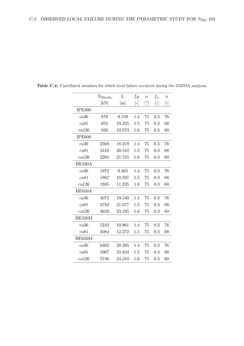
C.4. OBSERVED LOCAL FAILURE DURING THE PARAMETRIC STUDY FOR NRD 103
Table C.4: Castellated members for which local failure occurred during the GMNIA analyses.
NRd,abq L fH α fw n
[kN] [m] [-] [◦] [-] [-]
IPE300
ca36 879 9.159 1.4 75 0.3 76
ca81 853 10.255 1.5 75 0.3 68
ca126 826 10.873 1.6 75 0.3 60
IPE600
ca36 2569 18.319 1.4 75 0.3 76
ca81 2410 20.510 1.5 75 0.3 68
ca126 2294 21.745 1.6 75 0.3 60
HE320A
ca36 1972 9.465 1.4 75 0.3 76
ca81 1867 10.597 1.5 75 0.3 68
ca126 1935 11.235 1.6 75 0.3 60
HE650A
ca36 4074 19.540 1.4 75 0.3 76
ca81 3782 21.877 1.5 75 0.3 68
ca126 3629 23.195 1.6 75 0.3 60
HE320M
ca36 5243 10.961 1.4 75 0.3 76
ca81 5084 12.272 1.5 75 0.3 68
HE650M
ca36 6382 20.395 1.4 75 0.3 76
ca81 5907 22.834 1.5 75 0.3 68
ca126 5746 24.210 1.6 75 0.3 60

104 APPENDIX C. PARAMETRIC STUDY
Table C.5: Cellular members for which local failure occurred during the GMNIA analyses.
NRd,abq L fa fw n
[kN] [m] [-] [-] [-]
IPE300
c1 3107.30 9.048 0.8 0.1 34
IPE600
c1 2580.00 18.096 0.8 0.1 34
HE320A
c1 1962.16 9.350 0.8 0.1 34
c16 1924.23 10.323 1 0.1 30
c31 1905.73 11.16 1.2 0.1 27
HE650A
c1 4118.56 19.302 0.8 0.1 34
HE320M
c1 5272.64 10.827 0.8 0.1 34
c16 5204.64 11.9547 1 0.1 30
HE650M
c1 6487.21 20.147 0.8 0.1 34
C.5 Additional results for NRd
Table C.6: List of the cellular members for which NRd,abq exceeded Ncr,abq.
Ncr,abq NRd,abq L fa fw n
[kN] [kN] [m] [-] [-] [-]
IPE600 c5 452440 454914 91.0 0.8 0.1 172
IPE600 c10 455140 456345 88.6 0.8 0.4 131
IPE600 c20 432700 438436 99.2 1.0 0.1 150
IPE600 c25 432080 436562 96.5 1.0 0.4 114
IPE600 c30 421850 422558 89.0 1.0 0.7 86
IPE600 c35 412860 420776 107.1 1.2 0.1 135
IPE600 c40 412250 418045 103.7 1.2 0.4 102
HEM650 c20 1110500 1113223 110.4 1.0 0.1 150
HEM650 c25 1113300 1113836 107.4 1.0 0.4 114
HEM650 c35 1068100 1073009 119.3 1.2 0.1 135
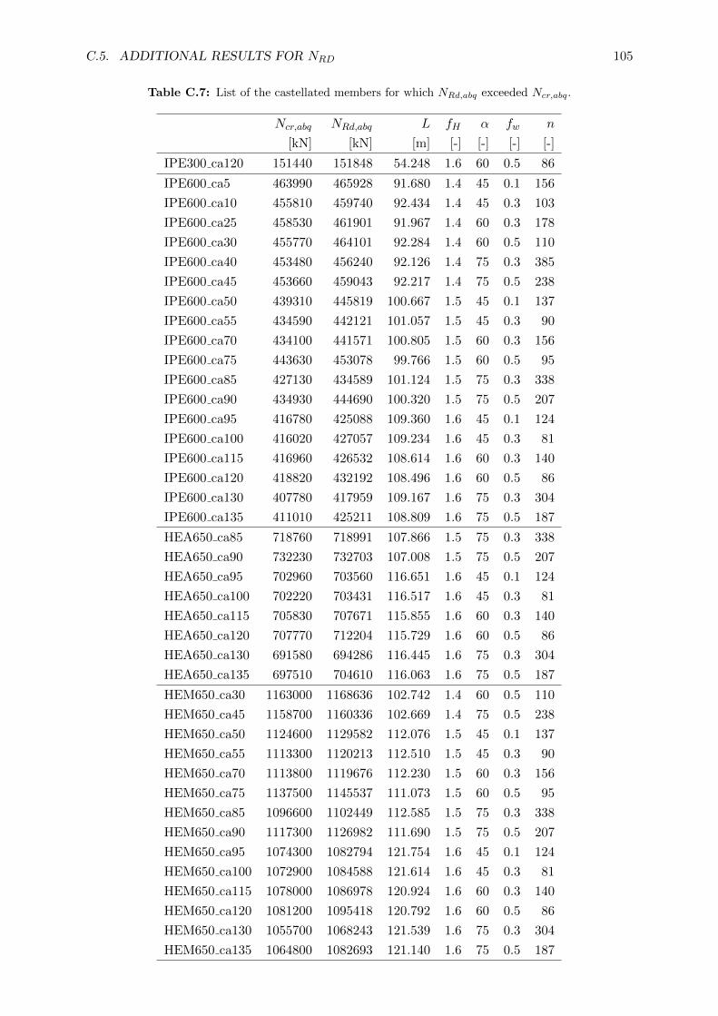
C.5. ADDITIONAL RESULTS FOR NRD 105
Table C.7: List of the castellated members for which NRd,abq exceeded Ncr,abq.
Ncr,abq NRd,abq L fH α fw n
[kN] [kN] [m] [-] [-] [-] [-]
IPE300 ca120 151440 151848 54.248 1.6 60 0.5 86
IPE600 ca5 463990 465928 91.680 1.4 45 0.1 156
IPE600 ca10 455810 459740 92.434 1.4 45 0.3 103
IPE600 ca25 458530 461901 91.967 1.4 60 0.3 178
IPE600 ca30 455770 464101 92.284 1.4 60 0.5 110
IPE600 ca40 453480 456240 92.126 1.4 75 0.3 385
IPE600 ca45 453660 459043 92.217 1.4 75 0.5 238
IPE600 ca50 439310 445819 100.667 1.5 45 0.1 137
IPE600 ca55 434590 442121 101.057 1.5 45 0.3 90
IPE600 ca70 434100 441571 100.805 1.5 60 0.3 156
IPE600 ca75 443630 453078 99.766 1.5 60 0.5 95
IPE600 ca85 427130 434589 101.124 1.5 75 0.3 338
IPE600 ca90 434930 444690 100.320 1.5 75 0.5 207
IPE600 ca95 416780 425088 109.360 1.6 45 0.1 124
IPE600 ca100 416020 427057 109.234 1.6 45 0.3 81
IPE600 ca115 416960 426532 108.614 1.6 60 0.3 140
IPE600 ca120 418820 432192 108.496 1.6 60 0.5 86
IPE600 ca130 407780 417959 109.167 1.6 75 0.3 304
IPE600 ca135 411010 425211 108.809 1.6 75 0.5 187
HEA650 ca85 718760 718991 107.866 1.5 75 0.3 338
HEA650 ca90 732230 732703 107.008 1.5 75 0.5 207
HEA650 ca95 702960 703560 116.651 1.6 45 0.1 124
HEA650 ca100 702220 703431 116.517 1.6 45 0.3 81
HEA650 ca115 705830 707671 115.855 1.6 60 0.3 140
HEA650 ca120 707770 712204 115.729 1.6 60 0.5 86
HEA650 ca130 691580 694286 116.445 1.6 75 0.3 304
HEA650 ca135 697510 704610 116.063 1.6 75 0.5 187
HEM650 ca30 1163000 1168636 102.742 1.4 60 0.5 110
HEM650 ca45 1158700 1160336 102.669 1.4 75 0.5 238
HEM650 ca50 1124600 1129582 112.076 1.5 45 0.1 137
HEM650 ca55 1113300 1120213 112.510 1.5 45 0.3 90
HEM650 ca70 1113800 1119676 112.230 1.5 60 0.3 156
HEM650 ca75 1137500 1145537 111.073 1.5 60 0.5 95
HEM650 ca85 1096600 1102449 112.585 1.5 75 0.3 338
HEM650 ca90 1117300 1126982 111.690 1.5 75 0.5 207
HEM650 ca95 1074300 1082794 121.754 1.6 45 0.1 124
HEM650 ca100 1072900 1084588 121.614 1.6 45 0.3 81
HEM650 ca115 1078000 1086978 120.924 1.6 60 0.3 140
HEM650 ca120 1081200 1095418 120.792 1.6 60 0.5 86
HEM650 ca130 1055700 1068243 121.539 1.6 75 0.3 304
HEM650 ca135 1064800 1082693 121.140 1.6 75 0.5 187

106 APPENDIX C. PARAMETRIC STUDY
Table C.8: Deviation betweenNRd,abq andNRd,i determined according to buckling curve i for castellated
members. The most appropriate buckling curve for each parent section is underlined.
IPE300 ∆min ∆max ∆mean ∆med∑
(χabq − χ)2
[ % ] [ % ] [ % ] [ % ] [-]
∆NRd,a -4.73 11.80 2.29 2.64 0.036
∆NRd,b -0.47 17.35 9.73 11.15 0.091
∆NRd,c 4.33 40.15 17.82 19.89 0.351
∆NRd,d 12.76 40.15 31.60 33.90 1.027
IPE600 ∆min ∆max ∆mean ∆med∑
(χabq − χ)2
[ % ] [ % ] [ % ] [ % ] [-]
∆NRd,a -3.90 13.30 3.78 4.05 0.028
∆NRd,b 0.42 18.90 11.40 12.53 0.114
∆NRd,c 5.29 42.10 19.67 21.68 0.390
∆NRd,d 13.83 42.10 33.78 36.12 1.064
HEA320 ∆min ∆max ∆mean ∆med∑
(χabq − χ)2
[ % ] [ % ] [ % ] [ % ] [-]
∆NRd,a -13.04 1.44 -4.91 -5.05 0.180
∆NRd,b -3.99 6.53 1.99 3.29 0.017
∆NRd,c 0.63 28.96 9.50 11.07 0.086
∆NRd,d 8.74 28.96 22.30 24.15 0.509
HEA650 ∆min ∆max ∆mean ∆med∑
(χabq − χ)2
[ % ] [ % ] [ % ] [ % ] [-]
∆NRd,a -5.49 11.84 2.01 2.28 0.048
∆NRd,b -1.27 17.39 9.42 11.01 0.081
∆NRd,c 3.50 39.52 17.48 19.78 0.321
∆NRd,d 11.86 39.52 31.23 33.88 0.970
HEM320 ∆min ∆max ∆mean ∆med∑
(χabq − χ)2
[ % ] [ % ] [ % ] [ % ] [-]
∆NRd,a -12.80 2.43 -4.36 -4.30 0.113
∆NRd,b -3.71 7.37 2.48 3.83 0.011
∆NRd,c 1.40 28.52 9.92 11.73 0.056
∆NRd,d 10.32 28.52 22.63 24.42 0.328
HEM650 ∆min ∆max ∆mean ∆med∑
(χabq − χ)2
[ % ] [ % ] [ % ] [ % ] [-]
∆NRd,a -5.49 11.99 2.32 2.54 0.047
∆NRd,b -1.18 17.47 9.72 11.29 0.083
∆NRd,c 3.68 39.72 17.77 20.15 0.322
∆NRd,d 12.21 39.72 31.50 33.92 0.968

C.5. ADDITIONAL RESULTS FOR NRD 107
Table C.9: Deviation between NRd,abq and NRd,i determined according to buckling curve i for cellular
members. The most appropriate buckling curve for each parent section is underlined.
IPE300 ∆min ∆max ∆mean ∆med∑
(χabq − χ)2
[ % ] [ % ] [ % ] [ % ] [-]
∆NRd,a -6.31 11.59 1.87 3.01 0.024
∆NRd,b -1.92 17.17 9.27 10.78 0.037
∆NRd,c 3.03 39.76 17.31 19.75 0.144
∆NRd,d 11.69 39.76 31.02 34.15 0.434
IPE600 ∆min ∆max ∆mean ∆med∑
(χabq − χ)2
[ % ] [ % ] [ % ] [ % ] [-]
∆NRd,a -5.42 13.49 3.26 3.95 0.019
∆NRd,b -1.03 19.26 10.76 12.22 0.049
∆NRd,c 3.92 41.82 18.92 21.48 0.170
∆NRd,d 12.59 41.82 32.84 35.89 0.481
HEA320 ∆min ∆max ∆mean ∆med∑
(χabq − χ)2
[ % ] [ % ] [ % ] [ % ] [-]
∆NRd,a -15.35 0.84 -5.94 -5.02 0.065
∆NRd,b -5.64 5.93 1.06 2.41 0.007
∆NRd,c 1.18 28.10 8.66 9.37 0.020
∆NRd,d 9.45 28.10 21.60 21.53 0.134
HEA650 ∆min ∆max ∆mean ∆med∑
(χabq − χ)2
[ % ] [ % ] [ % ] [ % ] [-]
∆NRd,a -6.82 10.48 1.33 2.49 0.030
∆NRd,b -2.52 16.06 8.72 10.43 0.034
∆NRd,c 2.33 39.23 16.75 19.17 0.133
∆NRd,d 10.83 39.23 30.43 33.50 0.414
HEM320 ∆min ∆max ∆mean ∆med∑
(χabq − χ)2
[ % ] [ % ] [ % ] [ % ] [-]
∆NRd,a -15.32 1.67 -5.12 -3.92 0.049
∆NRd,b -5.57 6.57 1.75 3.06 0.005
∆NRd,c 1.98 28.08 9.23 10.17 0.018
∆NRd,d 10.84 28.08 22.00 22.07 0.115
HEM650 ∆min ∆max ∆mean ∆med∑
(χabq − χ)2
[ % ] [ % ] [ % ] [ % ] [-]
∆NRd,a -6.75 11.45 1.80 2.85 0.028
∆NRd,b -2.35 17.00 9.18 10.98 0.035
∆NRd,c 2.61 39.39 17.21 19.71 0.135
∆NRd,d 11.27 39.39 30.89 33.89 0.416
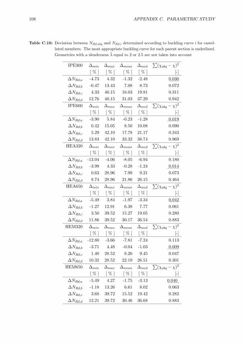
108 APPENDIX C. PARAMETRIC STUDY
Table C.10: Deviation between NRd,abq and NRd,i determined according to buckling curve i for castel-
lated members. The most appropriate buckling curve for each parent section is underlined.
Geometries with a slenderness λ equal to 2 or 2.5 are not taken into account
IPE300 ∆min ∆max ∆mean ∆med∑
(χabq − χ)2
[ % ] [ % ] [ % ] [ % ] [-]
∆NRd,a -4.73 4.32 -1.32 -2.48 0.030
∆NRd,b -0.47 13.43 7.08 8.73 0.072
∆NRd,c 4.33 40.15 16.03 19.81 0.311
∆NRd,d 12.76 40.15 31.03 37.29 0.942
IPE600 ∆min ∆max ∆mean ∆med∑
(χabq − χ)2
[ % ] [ % ] [ % ] [ % ] [-]
∆NRd,a -3.90 5.84 -0.23 -1.28 0.019
∆NRd,b 0.42 15.05 8.50 10.08 0.090
∆NRd,c 5.29 42.10 17.78 21.17 0.343
∆NRd,d 13.83 42.10 33.32 38.74 0.969
HEA320 ∆min ∆max ∆mean ∆med∑
(χabq − χ)2
[ % ] [ % ] [ % ] [ % ] [-]
∆NRd,a -13.04 -4.06 -8.05 -6.94 0.180
∆NRd,b -3.99 4.33 -0.28 -1.24 0.014
∆NRd,c 0.63 28.96 7.99 9.21 0.073
∆NRd,d 8.74 28.96 21.86 26.15 0.464
HEA650 ∆min ∆max ∆mean ∆med∑
(χabq − χ)2
[ % ] [ % ] [ % ] [ % ] [-]
∆NRd,a -5.49 3.84 -1.97 -3.34 0.042
∆NRd,b -1.27 12.91 6.38 7.77 0.061
∆NRd,c 3.50 39.52 15.27 19.05 0.280
∆NRd,d 11.86 39.52 30.17 36.54 0.883
HEM320 ∆min ∆max ∆mean ∆med∑
(χabq − χ)2
[ % ] [ % ] [ % ] [ % ] [-]
∆NRd,a -12.80 -3.66 -7.81 -7.24 0.113
∆NRd,b -3.71 4.48 -0.04 -1.03 0.009
∆NRd,c 1.40 28.52 8.26 9.45 0.047
∆NRd,d 10.32 28.52 22.19 26.51 0.301
HEM650 ∆min ∆max ∆mean ∆med∑
(χabq − χ)2
[ % ] [ % ] [ % ] [ % ] [-]
∆NRd,a -5.49 4.27 -1.75 -3.13 0.040
∆NRd,b -1.18 13.26 6.61 8.02 0.063
∆NRd,c 3.68 39.72 15.52 19.42 0.282
∆NRd,d 12.21 39.72 30.46 36.68 0.883
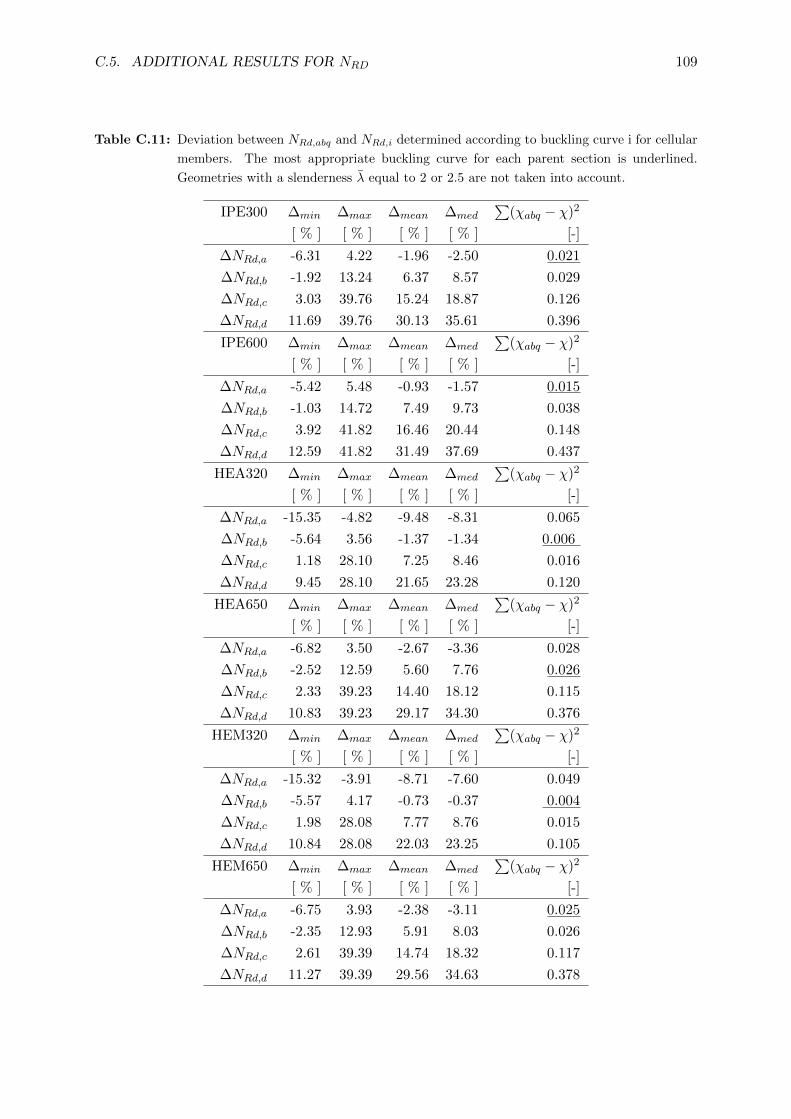
C.5. ADDITIONAL RESULTS FOR NRD 109
Table C.11: Deviation between NRd,abq and NRd,i determined according to buckling curve i for cellular
members. The most appropriate buckling curve for each parent section is underlined.
Geometries with a slenderness λ equal to 2 or 2.5 are not taken into account.
IPE300 ∆min ∆max ∆mean ∆med∑
(χabq − χ)2
[ % ] [ % ] [ % ] [ % ] [-]
∆NRd,a -6.31 4.22 -1.96 -2.50 0.021
∆NRd,b -1.92 13.24 6.37 8.57 0.029
∆NRd,c 3.03 39.76 15.24 18.87 0.126
∆NRd,d 11.69 39.76 30.13 35.61 0.396
IPE600 ∆min ∆max ∆mean ∆med∑
(χabq − χ)2
[ % ] [ % ] [ % ] [ % ] [-]
∆NRd,a -5.42 5.48 -0.93 -1.57 0.015
∆NRd,b -1.03 14.72 7.49 9.73 0.038
∆NRd,c 3.92 41.82 16.46 20.44 0.148
∆NRd,d 12.59 41.82 31.49 37.69 0.437
HEA320 ∆min ∆max ∆mean ∆med∑
(χabq − χ)2
[ % ] [ % ] [ % ] [ % ] [-]
∆NRd,a -15.35 -4.82 -9.48 -8.31 0.065
∆NRd,b -5.64 3.56 -1.37 -1.34 0.006
∆NRd,c 1.18 28.10 7.25 8.46 0.016
∆NRd,d 9.45 28.10 21.65 23.28 0.120
HEA650 ∆min ∆max ∆mean ∆med∑
(χabq − χ)2
[ % ] [ % ] [ % ] [ % ] [-]
∆NRd,a -6.82 3.50 -2.67 -3.36 0.028
∆NRd,b -2.52 12.59 5.60 7.76 0.026
∆NRd,c 2.33 39.23 14.40 18.12 0.115
∆NRd,d 10.83 39.23 29.17 34.30 0.376
HEM320 ∆min ∆max ∆mean ∆med∑
(χabq − χ)2
[ % ] [ % ] [ % ] [ % ] [-]
∆NRd,a -15.32 -3.91 -8.71 -7.60 0.049
∆NRd,b -5.57 4.17 -0.73 -0.37 0.004
∆NRd,c 1.98 28.08 7.77 8.76 0.015
∆NRd,d 10.84 28.08 22.03 23.25 0.105
HEM650 ∆min ∆max ∆mean ∆med∑
(χabq − χ)2
[ % ] [ % ] [ % ] [ % ] [-]
∆NRd,a -6.75 3.93 -2.38 -3.11 0.025
∆NRd,b -2.35 12.93 5.91 8.03 0.026
∆NRd,c 2.61 39.39 14.74 18.32 0.117
∆NRd,d 11.27 39.39 29.56 34.63 0.378

110 APPENDIX C. PARAMETRIC STUDY
Table C.12: Deviation between NRd,abq and NRd,i determined according to buckling curve i for castel-
lated members. The most appropriate buckling curve for each parent section is underlined.
Only geometries with a slenderness λ equal to 0.5 are taken into account.
IPE300 ∆min ∆max ∆mean ∆med∑
(χabq − χ)2
[%] [%] [%] [%] [-]
∆NRda -4.730 -3.401 -4.069 -4.150 0.0214
∆NRdb -0.472 0.990 0.320 0.172 0.0003
∆NRdc 4.335 15.391 5.271 5.189 0.0298
∆NRdd 12.763 15.391 13.942 14.034 0.1765
IPE600 ∆min ∆max ∆mean ∆med∑
(χabq − χ)2
[%] [%] [%] [%] [-]
∆NRda -3.903 -2.878 -3.547 -3.574 0.0130
∆NRdb 0.415 1.897 0.907 0.827 0.0009
∆NRdc 5.290 16.634 5.929 5.922 0.0300
∆NRdd 13.834 16.634 14.720 14.719 0.1567
HEA320 ∆min ∆max ∆mean ∆med∑
(χabq − χ)2
[%] [%] [%] [%] [-]
∆NRda -8.076 -5.996 -7.012 -6.941 0.0635
∆NRdb -3.985 -1.820 -2.826 -2.845 0.0098
∆NRdc 0.634 11.165 1.900 1.754 0.0043
∆NRdd 8.735 11.165 10.182 10.188 0.0951
HEA650 ∆min ∆max ∆mean ∆med∑
(χabq − χ)2
[%] [%] [%] [%] [-]
∆NRda -5.490 -4.173 -4.795 -4.794 0.0296
∆NRdb -1.269 0.253 -0.454 -0.531 0.0004
∆NRdc 3.498 14.465 4.442 4.454 0.0212
∆NRdd 11.856 14.465 13.020 12.968 0.1542
HEM320 ∆min ∆max ∆mean ∆med∑
(χabq − χ)2
[%] [%] [%] [%] [-]
∆NRda -8.259 -6.741 -7.288 -7.236 0.0450
∆NRdb -3.711 -2.256 -2.808 -2.805 0.0062
∆NRdc 1.399 11.613 2.232 2.320 0.0036
∆NRdd 10.316 11.613 11.036 11.319 0.0718
HEM650 ∆min ∆max ∆mean ∆med∑
(χabq − χ)2
[%] [%] [%] [%] [-]
∆NRda -5.495 -4.097 -4.723 -4.723 0.0286
∆NRdb -1.181 0.370 -0.276 -0.346 0.0003
∆NRdc 3.685 14.891 4.735 4.715 0.0238
∆NRdd 12.209 14.891 13.503 13.593 0.1640

C.5. ADDITIONAL RESULTS FOR NRD 111
Table C.13: Deviation between NRd,abq and NRd,i determined according to buckling curve i for cellular
members. The most appropriate buckling curve for each parent section is underlined. Only
geometries with a slenderness λ equal to 0.5 are taken into account.
IPE300 ∆min ∆max ∆mean ∆med∑
(χabq − χ)2
[%] [%] [%] [%] [-]
∆NRda -6.31 -4.19 -5.15 -5.14 0.0160
∆NRdb -1.92 0.38 -0.69 -0.57 0.0005
∆NRdc 3.03 14.54 4.34 4.34 0.0095
∆NRdd 11.69 14.54 13.12 12.94 0.0722
IPE600 ∆min ∆max ∆mean ∆med∑
(χabq − χ)2
[%] [%] [%] [%] [-]
∆NRda -5.42 -3.54 -4.34 -4.29 0.0114
∆NRdb -1.03 1.05 0.11 0.19 0.0002
∆NRdc 3.92 15.26 5.12 5.09 0.0132
∆NRdd 12.59 15.26 13.90 13.76 0.0813
HEA320 ∆min ∆max ∆mean ∆med∑
(χabq − χ)2
[%] [%] [%] [%] [-]
∆NRda -7.73 -7.03 -7.34 -7.26 0.0138
∆NRdb -3.54 -2.69 -3.11 -3.11 0.0023
∆NRdc 1.18 10.76 1.65 1.58 0.0006
∆NRdd 9.45 10.76 10.01 9.80 0.0182
HEA650 ∆min ∆max ∆mean ∆med∑
(χabq − χ)2
[%] [%] [%] [%] [-]
∆NRda -6.82 -4.65 -5.75 -5.94 0.0200
∆NRdb -2.52 -0.20 -1.41 -1.41 0.0014
∆NRdc 2.33 13.58 3.48 3.68 0.0063
∆NRdd 10.83 13.58 12.05 12.13 0.0616
HEM320 ∆min ∆max ∆mean ∆med∑
(χabq − χ)2
[%] [%] [%] [%] [-]
∆NRda -7.60 -7.44 -7.53 -7.56 0.0143
∆NRdb -3.09 -2.89 -2.97 -2.94 0.0020
∆NRdc 1.98 11.48 2.15 2.12 0.0010
∆NRdd 10.84 11.48 11.09 10.96 0.0215
HEM650 ∆min ∆max ∆mean ∆med∑
(χabq − χ)2
[%] [%] [%] [%] [-]
∆NRda -6.75 -4.60 -5.51 -5.41 0.0183
∆NRdb -2.35 -0.03 -1.06 -0.89 0.0009
∆NRdc 2.61 14.08 3.96 4.01 0.0080
∆NRdd 11.27 14.08 12.73 12.61 0.0679

112 APPENDIX C. PARAMETRIC STUDY

Appendix D
Further research towards design
rules
D.1 Evaluation of the deviation between Ncr,abq and Ncr,2T
Fig. D.1 and D.2 display the deviation between Ncr,abq and Ncr,2T according to Eq. D.1 for
cellular and castellated columns respectively. The largest deviations occur for members with
an equivalent slenderness λ equal to 0.5 (see Fig. D.3 and D.4), which corresponds to lengths
smaller than approximately 20 m. These members will be investigated further to determine the
influence of the geometry of the member on the critical buckling load. Based on those results, a
design rule will be proposed for the critical buckling load Ncr. It is based on Ncr,2T multiplied
with a reduction factor, as a comparison between Ncr,2T and Ncr,abq illustrated that Ncr,2T
overestimates the critical buckling load (the deviation ∆Ncr,2Tin Fig. D.1 and D.2 is negative,
which indicates that Ncr,2T is larger than Ncr,abq).
∆Ncr,2T=
(Ncr,abq
Ncr,2T− 1
)· 100 (D.1)
D.1.1 Influence of the width of the web post
The width of the web post w is determined as in Eq. D.2 for cellular members and as in Eq. D.3
for castellated members. a stands for the height of the opening and c is the length of the inclined
part of a hexagonal opening. The geometry of cellular and castellated members is discussed in
section 2.3.
w = fw · a (D.2)
w = fw`0 = fw(w + 2c) (D.3)
Cellular columns
In Table D.5, the specifications of the different geometries and the deviation ∆Ncr,2Tare given
for cellular columns with λ = 0.5. The geometries for which the largest deviation occurs (c16
and c31) are summarized in Table D.1. In this table there are no members based on parent
113

114 APPENDIX D. FURTHER RESEARCH TOWARDS DESIGN RULES
0 20 40 60 80 100 120
Length [m]
−30
−20
−10
0
10
20
30
∆N
2T
=Ncr,abq/N
cr,2T−
1[%
]
Cellular columns
IPE300IPE600HE320AHE650AHE320MHE650M
Figure D.1: Deviation between Ncr,abq and Ncr,2T for cellular columns.
0 20 40 60 80 100 120
Length [m]
−30
−20
−10
0
10
20
30
∆N
2T
=Ncr,abq/N
cr,2T−
1[%
]
Castellated columns
IPE300IPE600HE320AHE650AHE320MHE650M
Figure D.2: Deviation between Ncr,abq and Ncr,2T for castellated columns.

D.1. EVALUATION OF THE DEVIATION BETWEEN NCR,ABQ AND NCR,2T 115
0.0 0.5 1.0 1.5 2.0 2.5 3.0
λ [-]
−30
−20
−10
0
10
20
30
∆Ncr,
2T
=Ncr,abq/N
cr,2T−
1[%
]
Cellular columns
IPE300IPE600HE320AHE650AHE320MHE650M
Figure D.3: Deviation between Ncr,abq and Ncr,2T for cellular columns, in function of λ.
0.0 0.5 1.0 1.5 2.0 2.5 3.0
λ [-]
−30
−20
−10
0
10
20
30
∆Ncr,
2T
=Ncr,abq/N
cr,2T−
1[%
]
Castellated columns
IPE300IPE600HE320AHE650AHE320MHE650M
Figure D.4: Deviation between Ncr,abq and Ncr,2T for castellated columns, in function of λ.

116 APPENDIX D. FURTHER RESEARCH TOWARDS DESIGN RULES
sections HE320A and HE320M as for geometries c16 and c31 of those parent sections local
failure occurred in the GMNIA analyses. Hence, they are not further considered.
Geometries c16 and c31 have the factor fw = 0.1 in common which results in the smallest
width of the web post of all geometries considered for cellular columns. As such, the deformation
of the web post is larger for those geometries than for the others, resulting in a lower critical
buckling load. This is not taken into account in the determination of Ncr,2T , so that Ncr,2T is at
most 26% larger than the numerically obtained Ncr,abq (for HE650A c31). Hence, the influence
of the width of the web post should be taken into account in a reduction factor for Ncr,2T .
Table D.1: Summary of the cellular members with λ = 0.5 and with the largest deviation ∆Ncr,2T.
IPE300 fa fw a [m] w [m] H [m] L [m] ∆Ncr,2T[%]
c16 1.00 0.10 0.300 0.030 0.441 9.990 -22.91
c31 1.20 0.10 0.360 0.036 0.471 10.800 -24.01
IPE600 fa fw a [m] w [m] H [m] L [m] ∆Ncr,2T[%]
c16 1.00 0.10 0.600 0.060 0.890 19.980 -19.31
c31 1.20 0.10 0.720 0.072 0.950 21.600 -19.85
HEA650 fa fw a [m] w [m] H [m] L [m] ∆Ncr,2T[%]
c16 1.00 0.10 0.640 0.064 0.950 21.312 -25.68
c31 1.20 0.10 0.768 0.077 1.014 23.040 -26.92
HEM650 fa fw a [m] w [m] H [m] L [m] ∆Ncr,2T[%]
c16 1.00 0.10 0.668 0.067 0.992 22.244 -24.85
c31 1.20 0.10 0.802 0.080 1.059 24.048 -25.99
Castellated columns
In Tables D.6 and D.7, the specifications of the different geometries and the deviation ∆Ncr,2T
are given for castellated columns with λ = 0.5. The geometries for which the largest deviation
occurs (ca116 and ca131) are summarized in Table D.2. In this table there are no members
based on parent section HE320M because the geometric constraints mentioned in section 2.4 are
not fulfilled for geometries with fH = 1.6 for this parent section. Hence, they are not further
considered.
For geometry ca116 (fH = 1.6, α = 60◦ and fw = 0.5) is the width of the web post w the
largest of all the considered geometries. Geometry ca131 (fH = 1.6, α = 75◦ and fw = 0.5)
results in the smallest length c of the inclined part of the hexagonal opening for fH = 1.6 (fH
indicates the increased height H of the castellated member). The largest deviations between
Ncr,abq and Ncr,2T occur thus for geometries with wide web posts paired with a large angle α
(which results in small lengths c of the inclined part of the hexagonal opening) and for geometries
that result in the largest increase in height H (fH = 1.6). This does not comply with what was
found for cellular columns.
However, the largest deviations for castellated columns with a slenderness λ equal to 1.0
occur for those geometries that result in the smallest c and the smallest w (see Table D.3),
regardless of the value of fH , which does agree with the conclusion drawn for cellular columns.
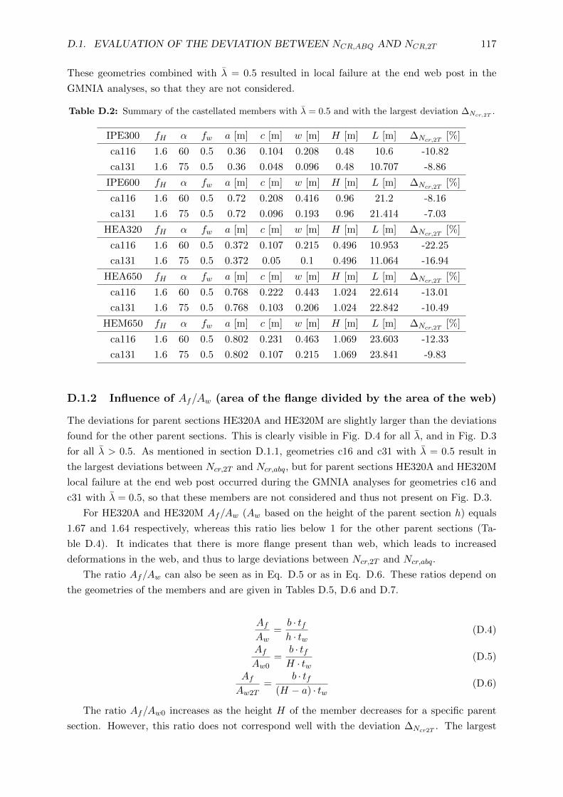
D.1. EVALUATION OF THE DEVIATION BETWEEN NCR,ABQ AND NCR,2T 117
These geometries combined with λ = 0.5 resulted in local failure at the end web post in the
GMNIA analyses, so that they are not considered.
Table D.2: Summary of the castellated members with λ = 0.5 and with the largest deviation ∆Ncr,2T.
IPE300 fH α fw a [m] c [m] w [m] H [m] L [m] ∆Ncr,2T[%]
ca116 1.6 60 0.5 0.36 0.104 0.208 0.48 10.6 -10.82
ca131 1.6 75 0.5 0.36 0.048 0.096 0.48 10.707 -8.86
IPE600 fH α fw a [m] c [m] w [m] H [m] L [m] ∆Ncr,2T[%]
ca116 1.6 60 0.5 0.72 0.208 0.416 0.96 21.2 -8.16
ca131 1.6 75 0.5 0.72 0.096 0.193 0.96 21.414 -7.03
HEA320 fH α fw a [m] c [m] w [m] H [m] L [m] ∆Ncr,2T[%]
ca116 1.6 60 0.5 0.372 0.107 0.215 0.496 10.953 -22.25
ca131 1.6 75 0.5 0.372 0.05 0.1 0.496 11.064 -16.94
HEA650 fH α fw a [m] c [m] w [m] H [m] L [m] ∆Ncr,2T[%]
ca116 1.6 60 0.5 0.768 0.222 0.443 1.024 22.614 -13.01
ca131 1.6 75 0.5 0.768 0.103 0.206 1.024 22.842 -10.49
HEM650 fH α fw a [m] c [m] w [m] H [m] L [m] ∆Ncr,2T[%]
ca116 1.6 60 0.5 0.802 0.231 0.463 1.069 23.603 -12.33
ca131 1.6 75 0.5 0.802 0.107 0.215 1.069 23.841 -9.83
D.1.2 Influence of Af/Aw (area of the flange divided by the area of the web)
The deviations for parent sections HE320A and HE320M are slightly larger than the deviations
found for the other parent sections. This is clearly visible in Fig. D.4 for all λ, and in Fig. D.3
for all λ > 0.5. As mentioned in section D.1.1, geometries c16 and c31 with λ = 0.5 result in
the largest deviations between Ncr,2T and Ncr,abq, but for parent sections HE320A and HE320M
local failure at the end web post occurred during the GMNIA analyses for geometries c16 and
c31 with λ = 0.5, so that these members are not considered and thus not present on Fig. D.3.
For HE320A and HE320M Af/Aw (Aw based on the height of the parent section h) equals
1.67 and 1.64 respectively, whereas this ratio lies below 1 for the other parent sections (Ta-
ble D.4). It indicates that there is more flange present than web, which leads to increased
deformations in the web, and thus to large deviations between Ncr,2T and Ncr,abq.
The ratio Af/Aw can also be seen as in Eq. D.5 or as in Eq. D.6. These ratios depend on
the geometries of the members and are given in Tables D.5, D.6 and D.7.
AfAw
=b · tfh · tw
(D.4)
AfAw0
=b · tfH · tw
(D.5)
AfAw2T
=b · tf
(H − a) · tw(D.6)
The ratio Af/Aw0 increases as the height H of the member decreases for a specific parent
section. However, this ratio does not correspond well with the deviation ∆Ncr2T. The largest

118 APPENDIX D. FURTHER RESEARCH TOWARDS DESIGN RULES
Table D.3: Summary of the castellated members with λ = 1.0 and with the largest deviation ∆Ncr,2T.
IPE300 fH α fw a [m] c [m] w [m] H [m] L [m] ∆Ncr,2T[%]
ca37 1.4 75 0.3 0.240 0.032 0.028 0.420 18.236 -2.90
ca82 1.5 75 0.3 0.300 0.040 0.034 0.450 20.108 -2.34
ca127 1.6 75 0.3 0.360 0.048 0.041 0.480 21.621 -1.99
IPE600 fH α fw a [m] c [m] w [m] H [m] L [m] ∆Ncr,2T[%]
ca37 1.4 75 0.3 0.480 0.064 0.055 0.840 36.472 -2.25
ca82 1.5 75 0.3 0.600 0.080 0.069 0.900 40.215 -1.68
ca127 1.6 75 0.3 0.720 0.096 0.083 0.960 43.242 -1.10
HEA320 fH α fw a [m] c [m] w [m] H [m] L [m] ∆Ncr,2T[%]
ca37 1.4 75 0.3 0.248 0.033 0.028 0.434 18.844 -6.06
ca82 1.5 75 0.3 0.310 0.042 0.036 0.465 20.778 -5.78
ca127 1.6 75 0.3 0.372 0.050 0.043 0.496 22.342 -5.83
HEA650 fH α fw a [m] c [m] w [m] H [m] L [m] ∆Ncr,2T[%]
ca37 1.4 75 0.3 0.512 0.069 0.059 0.896 38.903 -3.52
ca82 1.5 75 0.3 0.640 0.086 0.073 0.960 42.896 -3.11
ca127 1.6 75 0.3 0.768 0.103 0.088 1.024 46.125 -2.69
HEM320 fH α fw a [m] c [m] w [m] H [m] L [m] ∆Ncr,2T[%]
ca37 1.4 75 0.3 0.287 0.038 0.033 0.503 21.822 -5.81
ca82 1.5 75 0.3 0.359 0.048 0.041 0.539 24.062 -5.61
HEM650 fH α fw a [m] c [m] w [m] H [m] L [m] ∆Ncr,2T[%]
ca37 1.4 75 0.3 0.534 0.072 0.061 0.935 40.605 -3.33
ca82 1.5 75 0.3 0.668 0.089 0.077 1.002 44.773 -2.83
ca127 1.6 75 0.3 0.802 0.107 0.092 1.069 48.143 -2.49
Table D.4: Af/Aw for the different parent sections.
IPE300 IPE600 HE320A HE650A HE320M HE650M
Af/Aw 0.75 0.58 1.67 0.9 1.64 0.87
D.2. PRELIMINARY PROPOSAL FOR ADESIGN RULE TODETERMINE THE CRITICAL BUCKLING LOAD119
deviation is noticed for geometries c16 and c31 for cellular columns; for those geometries the
width of the web post w is the smallest. For geometry c31 Af/Aw0 is the smallest, whereas the
ratio is in the middle for geometry c16. This is logical as geometry c31 results in the highest
height H of all considered geometries, and thus results in the smallest ratio Af/Aw0: the only
parameter that changes in this ratio for the different geometries is H. As the width of the web
post is not taken into account in Af/Aw0, the ratio found for geometry c16 lies in the middle
of the ratios found for the different geometries. Additionally, for each parent section there is a
variation in the deviation ∆Ncr2Tof about 15%. The variation in the ratio Af/Aw0 is only about
10%.
For castellated columns the ratio Af/Aw0 only depends on fH , so that there is no influence
of the shape of the opening. As such, little agreement is found between Af/Aw0 and ∆Ncr2T
for castellated members. Yet, the ratio is still larger than 1 for parent sections HE320A and
HE320M, and below 1 for the other parent sections, both for castellated and cellular columns.
The ratio Af/Aw2T is also only depended of fH , as both the height H and the height of the
hexagonal opening a are determined with this factor for castellated members. As such, little
agreement is found with the deviation ∆Ncr2T. For cellular members however the geometry of
the opening does influence Af/Aw2T . Yet, there is a variation between the different geometries
of almost 1, and the largest ratio Af/Aw2T does not occur for the geometry with the largest
deviation ∆Ncr2T. Hence it can be concluded that this ratio will not be helpful for the proposal
of a reduction factor for Ncr,2T .
D.2 Preliminary proposal for a design rule to determine the
critical buckling load
The aim is to find an equation that accurately predicts the critical buckling load of castellated
and cellular members. For longer members (with slenderness λ > 0.5), the deviation between
Ncr,2T and Ncr,abq is deemed acceptable (see Fig. D.3 and D.4), so that a reduction factor will
only be applied on Ncr,2T for members that have a slenderness equal to 0.5.
As it is pointed out in section D.1.1 that the width of the web post w has a large influence
on the deviation ∆Ncr,2T, the ratio nw/L is considered first. It is the width of all the web posts
combined, divided by the total length of the member. The values of nw/L for the different
geometries can be found in Tables D.5, D.6 and D.7. nw/L is the same for each considered
geometry, regardless of the parent section. This is illustrated in Eq. D.7 for cellular members.
There is a difference of 0.3 between the maximum and minimum value found for nw/L and the
minimum value is found for c16 and c31, the maximum value for c11. For those geometries,
the most and the least reduction is required of Ncr,2T respectively. However, for castellated
members, little agreement is found between the deviation ∆Ncr,2Tand the ratio nw/L. It was
already indicated in section D.1.1 that the deviation for castellated columns was not largest for
the members with the smallest width of the web post w, and it is confirmed by the values of
nw/L.
nw
L=
nfwa
n · a+ (n− 1)w + 2 ·wend=
nfwfah
nfah+ (n+ 3)fwfah=
nfwfanfa + (n+ 3)fwfa
(D.7)

120 APPENDIX D. FURTHER RESEARCH TOWARDS DESIGN RULES
Another way to take the geometry of the openings into account is by considering the ratio
of the area of the web to the area of the unperforated web (Eq. D.8 for cellular columns and
Eq. D.9 for castellated columns). For this ratio, again a good agreement is found with the
deviation found for cellular columns: the lowest value occurs for those geometries that have a
large deviation between Ncr,abq and Ncr,2T . The same can not be said for castellated columns,
although the ratios found for geometries ca116 and ca131 are among the lowest values found
for the different geometries. So far, this is the ratio which results in the closest agreement
with the deviation ∆Ncr,2T. Yet, it does not account for the differences between the different
parent sections nor is there as much variation between the extreme values as there is between
the extreme values of the deviation.
hwebL− nπa2
4
hwebL(D.8)
hwebL− n(c+ w)a
hwebL(D.9)
The idea for the design rule is to multiply Ncr,2T with the ratios mentioned in Eq. D.8
and D.9 for cellular and castellated columns respectively (this is only done for members with
a slenderness λ = 0.5). However, as the maximum value of this ratio equals 0.72, this might
result in values for the critical buckling load that are almost 30% smaller than Ncr,abq obtained in
Abaqus which would be very conservative. As such, Ncr,2T will be multiplied with the mentioned
ratio augmented by a certain factor as in Eq. D.10 and D.11. The deviation between the thus
obtained critical buckling load and the critical buckling load obtained in Abaqus Ncr,abq is
displayed in Fig. D.5 and D.6. In these graphs, ’factor’ is taken equal to 0.28 as this value
resulted in the smallest variation about a deviation equal to 0% (1= 0.28+0.72 (the maximum
value of Eq. D.8 or Eq. D.9)). Yet, this value is arbitrarily determined so that more research
regarding this ’factor’ is recommended. Also, the differences that occur between the different
parent sections are not taken into account in the determination of the critical buckling load,
which should actually be done to determine a more accurate prediction of the critical buckling
load. To be able to incorporate this in the design rule more research should be conducted.
Ncr,proposal =
(hwebL− nπa2
4
hwebL+ factor
)π2EI2TL2cr
(D.10)
Ncr,proposal =
(hwebL− n(c+ w)a
hwebL+ factor
)π2EI2TL2cr
(D.11)
D.3 Conclusions
From an evaluation of the deviation between Ncr,abq and Ncr,2T it could be concluded that larger
deviations arise for parent sections HE320A and HE320M. This is reflected in the ratio Af/Aw
which is larger than 1 for those parent sections and below 1 for the other parent sections. It
indicates that the flanges are heavier than the web of the sections, leading to increased defor-
mations in the web and thus to a lower critical buckling load than the numerically determined
Ncr,2T .

D.3. CONCLUSIONS 121
0 20 40 60 80 100 120
Length [m]
−30
−20
−10
0
10
20
30
∆Nproposal=Ncr,abq/N
cr,proposal−
1[%
]Cellular columns
IPE300IPE600HE320AHE650AHE320MHE650M
Figure D.5: Deviation between Ncr,abq and Ncr,proposal for cellular columns.
0 20 40 60 80 100 120
Length [m]
−30
−20
−10
0
10
20
30
∆Nproposal=Ncr,abq/N
cr,proposal−
1[%
]
Castellated columns
IPE300IPE600HE320AHE650AHE320MHE650M
Figure D.6: Deviation between Ncr,abq and Ncr,proposal for castellated columns.
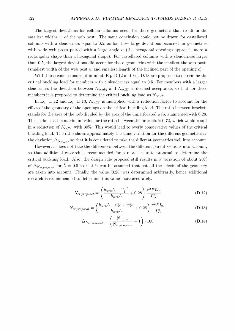
122 APPENDIX D. FURTHER RESEARCH TOWARDS DESIGN RULES
The largest deviations for cellular columns occur for those geometries that result in the
smallest widths w of the web post. The same conclusion could not be drawn for castellated
columns with a slenderness equal to 0.5, as for those large deviations occurred for geometries
with wide web posts paired with a large angle α (the hexagonal openings approach more a
rectangular shape than a hexagonal shape). For castellated columns with a slenderness larger
than 0.5, the largest deviations did occur for those geometries with the smallest the web posts
(smallest width of the web post w and smallest length of the inclined part of the opening c).
With those conclusions kept in mind, Eq. D.12 and Eq. D.13 are proposed to determine the
critical buckling load for members with a slenderness equal to 0.5. For members with a larger
slenderness the deviation between Ncr,abq and Ncr,2T is deemed acceptable, so that for those
members it is proposed to determine the critical buckling load as Ncr,2T .
In Eq. D.12 and Eq. D.13, Ncr,2T is multiplied with a reduction factor to account for the
effect of the geometry of the openings on the critical buckling load. The ratio between brackets
stands for the area of the web divided by the area of the unperforated web, augmented with 0.28.
This is done as the maximum value for the ratio between the brackets is 0.72, which would result
in a reduction of Ncr,2T with 30%. This would lead to overly conservative values of the critical
buckling load. The ratio shows approximately the same variation for the different geometries as
the deviation ∆Ncr,2T, so that it is considered to take the different geometries well into account.
However, it does not take the differences between the different parent sections into account,
so that additional research is recommended for a more accurate proposal to determine the
critical buckling load. Also, the design rule proposal still results in a variation of about 20%
of ∆Ncr,proposalfor λ = 0.5 so that it can be assumed that not all the effects of the geometry
are taken into account. Finally, the value ’0.28’ was determined arbitrarily, hence additional
research is recommended to determine this value more accurately.
Ncr,proposal =
(hwebL− nπa2
4
hwebL+ 0.28
)π2EI2TL2cr
(D.12)
Ncr,proposal =
(hwebL− n(c+ w)a
hwebL+ 0.28
)π2EI2TL2cr
(D.13)
∆Ncr,proposal=
(Ncr,abq
Ncr,proposal− 1
)· 100 (D.14)

D.3. CONCLUSIONS 123
Table D.5: Geometries with λ = 0.5 for cellular columns.
IPE300 fa fw a [m] w [m] H [m] L [m] ∆Ncr2T[%] Af/Aw0 Af/Aw2T nw/L Eq.D.8
c6 0.8 0.4 0.240 0.096 0.401 9.024 -6.34 0.58 1.50 0.28 0.67
c11 0.8 0.7 0.240 0.168 0.374 8.256 -4.82 0.62 1.83 0.39 0.71
c16 1.0 0.1 0.300 0.030 0.441 9.990 -22.91 0.53 1.73 0.09 0.51
c21 1.0 0.4 0.300 0.120 0.429 9.600 -7.35 0.54 1.92 0.28 0.61
c26 1.0 0.7 0.300 0.210 0.396 9.300 -5.59 0.59 2.66 0.38 0.66
c31 1.2 0.1 0.360 0.036 0.471 10.800 -24.01 0.49 2.25 0.09 0.45
c36 1.2 0.4 0.360 0.144 0.456 10.512 -9.36 0.51 2.64 0.27 0.57
IPE600 fa fw a [m] w [m] H [m] L [m] ∆Ncr2T[%] Af/Aw0 Af/Aw2T nw/L Eq.D.8
c6 0.8 0.4 0.480 0.192 0.811 18.048 -4.87 0.44 1.12 0.28 0.67
c11 0.8 0.7 0.480 0.336 0.760 16.512 -3.29 0.47 1.33 0.39 0.72
c16 1.0 0.1 0.600 0.060 0.890 19.980 -19.31 0.40 1.28 0.09 0.51
c21 1.0 0.4 0.600 0.240 0.866 19.200 -5.30 0.41 1.41 0.28 0.62
c26 1.0 0.7 0.600 0.420 0.803 18.600 -3.15 0.44 1.89 0.38 0.67
c31 1.2 0.1 0.720 0.072 0.950 21.600 -19.85 0.37 1.65 0.09 0.45
c36 1.2 0.4 0.720 0.288 0.921 21.024 -6.35 0.39 1.91 0.27 0.57
HEA320 fa fw a [m] w [m] H [m] L [m] ∆Ncr2T[%] Af/Aw0 Af/Aw2T nw/L Eq.D.8
c6 0.8 0.4 0.248 0.099 0.415 9.325 -12.81 1.29 3.41 0.28 0.66
c11 0.8 0.7 0.248 0.174 0.387 8.531 -11.15 1.39 4.19 0.39 0.71
c21 1.0 0.4 0.310 0.124 0.443 9.920 -15.47 1.21 4.39 0.28 0.61
HEA650 fa fw a [m] w [m] H [m] L [m] ∆Ncr2T[%] Af/Aw0 Af/Aw2T nw/L Eq.D.8
c6 0.8 0.4 0.512 0.205 0.866 19.251 -7.50 0.69 1.76 0.28 0.67
c11 0.8 0.7 0.512 0.358 0.811 17.613 -5.93 0.74 2.11 0.39 0.72
c16 1.0 0.1 0.640 0.064 0.950 21.312 -25.68 0.63 2.03 0.09 0.51
c21 1.0 0.4 0.640 0.256 0.925 20.480 -8.73 0.64 2.23 0.28 0.62
c26 1.0 0.7 0.640 0.448 0.857 19.840 -6.87 0.70 3.02 0.38 0.67
c31 1.2 0.1 0.768 0.077 1.014 23.040 -26.92 0.58 2.63 0.09 0.45
c36 1.2 0.4 0.768 0.307 0.983 22.426 -10.91 0.60 3.05 0.27 0.57
HEM320 fa fw a [m] w [m] H [m] L [m] ∆Ncr2T[%] Af/Aw0 Af/Aw2T nw/L Eq.D.8
c6 0.8 0.4 0.287 0.115 0.482 10.799 -11.72 1.33 3.81 0.28 0.65
c11 0.8 0.7 0.287 0.201 0.450 9.880 -9.61 1.44 4.79 0.39 0.70
c21 1.0 0.4 0.359 0.144 0.515 11.488 -13.49 1.24 5.08 0.28 0.59
HEM650 fa fw a [m] w [m] H [m] L [m] ∆Ncr2T[%] Af/Aw0 Af/Aw2T nw/L Eq.D.8
c6 0.8 0.4 0.534 0.214 0.904 20.093 -7.11 0.67 1.76 0.28 0.66
c11 0.8 0.7 0.534 0.374 0.847 18.383 -5.53 0.72 2.13 0.39 0.71
c16 1.0 0.1 0.668 0.067 0.992 22.244 -24.85 0.61 2.04 0.09 0.50
c21 1.0 0.4 0.668 0.267 0.965 21.376 -8.24 0.63 2.26 0.28 0.61
c26 1.0 0.7 0.668 0.468 0.895 20.708 -6.25 0.68 3.10 0.38 0.66
c31 1.2 0.1 0.802 0.080 1.059 24.048 -25.99 0.57 2.68 0.09 0.44
c36 1.2 0.4 0.802 0.321 1.027 23.407 -10.23 0.59 3.14 0.27 0.56

124 APPENDIX D. FURTHER RESEARCH TOWARDS DESIGN RULES
Table D.6: Geometries with λ = 0.5 for castellated columns.
IPE300 fH α fw a [m] c [m] w [m] H [m] L [m] ∆Ncr2T[%] Af/Aw0 Af/Aw2T nw/L Eq.D.9
ca1 1.4 45 0.1 0.240 0.120 0.027 0.420 9.173 -5.43 0.55 1.34 0.09 0.71
ca6 1.4 45 0.3 0.240 0.120 0.103 0.420 9.223 -4.73 0.55 1.34 0.22 0.72
ca21 1.4 60 0.3 0.240 0.069 0.059 0.420 9.185 -5.49 0.55 1.34 0.23 0.71
ca26 1.4 60 0.5 0.240 0.069 0.139 0.420 9.145 -5.39 0.55 1.34 0.32 0.72
ca41 1.4 75 0.5 0.240 0.032 0.064 0.420 9.453 -7.40 0.55 1.34 0.33 0.71
ca46 1.5 45 0.1 0.300 0.150 0.033 0.450 10.000 -4.92 0.51 1.62 0.09 0.66
ca51 1.5 45 0.3 0.300 0.150 0.129 0.450 9.857 -5.58 0.51 1.62 0.22 0.67
ca66 1.5 60 0.3 0.300 0.087 0.074 0.450 9.873 -5.63 0.51 1.62 0.23 0.67
ca71 1.5 60 0.5 0.300 0.087 0.173 0.450 9.873 -6.88 0.51 1.62 0.32 0.68
ca86 1.5 75 0.5 0.300 0.040 0.080 0.450 10.128 -7.65 0.51 1.62 0.33 0.67
ca91 1.6 45 0.1 0.360 0.180 0.040 0.480 10.680 -4.71 0.48 2.07 0.09 0.62
ca96 1.6 45 0.3 0.360 0.180 0.154 0.480 11.160 -6.66 0.48 2.07 0.22 0.63
ca111 1.6 60 0.3 0.360 0.104 0.089 0.480 11.075 -5.57 0.48 2.07 0.23 0.63
ca116 1.6 60 0.5 0.360 0.104 0.208 0.480 10.600 -10.82 0.48 2.07 0.31 0.64
ca131 1.6 75 0.5 0.360 0.048 0.096 0.480 10.707 -8.86 0.48 2.07 0.32 0.63
IPE600 fH α fw a [m] c [m] w [m] H [m] L [m] ∆Ncr2T[%] Af/Aw0 Af/Aw2T nw/L Eq.D.9
ca21 1.4 60 0.3 0.480 0.139 0.119 0.840 18.370 -4.34 0.42 1.02 0.23 0.71
ca41 1.4 75 0.5 0.480 0.064 0.129 0.840 18.906 -6.09 0.42 1.02 0.33 0.71
ca46 1.5 45 0.1 0.600 0.300 0.067 0.900 20.000 -3.30 0.40 1.24 0.09 0.66
ca51 1.5 45 0.3 0.600 0.300 0.257 0.900 19.714 -3.96 0.40 1.24 0.22 0.67
ca66 1.5 60 0.3 0.600 0.173 0.148 0.900 19.745 -4.20 0.40 1.24 0.23 0.67
ca71 1.5 60 0.5 0.600 0.173 0.346 0.900 19.745 -5.21 0.40 1.24 0.32 0.68
ca86 1.5 75 0.5 0.600 0.080 0.161 0.900 20.257 -6.19 0.40 1.24 0.33 0.67
ca91 1.6 45 0.1 0.720 0.360 0.080 0.960 21.360 -2.72 0.37 1.58 0.09 0.62
ca96 1.6 45 0.3 0.720 0.360 0.309 0.960 22.320 -4.44 0.37 1.58 0.22 0.63
ca111 1.6 60 0.3 0.720 0.208 0.178 0.960 22.150 -3.87 0.37 1.58 0.23 0.63
ca116 1.6 60 0.5 0.720 0.208 0.416 0.960 21.200 -8.16 0.37 1.58 0.31 0.64
ca131 1.6 75 0.5 0.720 0.096 0.193 0.960 21.414 -7.03 0.37 1.58 0.32 0.63
HEA320 fH α fw a [m] c [m] w [m] H [m] L [m] ∆Ncr2T[%] Af/Aw0 Af/Aw2T nw/L Eq.D.9
ca1 1.4 45 0.1 0.248 0.124 0.028 0.434 9.479 -11.25 1.23 3.03 0.09 0.71
ca6 1.4 45 0.3 0.248 0.124 0.106 0.434 9.530 -9.95 1.23 3.03 0.22 0.71
ca21 1.4 60 0.3 0.248 0.072 0.061 0.434 9.491 -10.90 1.23 3.03 0.23 0.71
ca26 1.4 60 0.5 0.248 0.072 0.143 0.434 9.450 -10.80 1.23 3.03 0.32 0.72
ca41 1.4 75 0.5 0.248 0.033 0.066 0.434 9.768 -13.72 1.23 3.03 0.33 0.71
ca46 1.5 45 0.1 0.310 0.155 0.034 0.465 10.333 -11.45 1.15 3.70 0.09 0.66
ca51 1.5 45 0.3 0.310 0.155 0.133 0.465 10.186 -12.46 1.15 3.70 0.22 0.67
ca66 1.5 60 0.3 0.310 0.089 0.077 0.465 10.202 -11.78 1.15 3.70 0.23 0.66
ca71 1.5 60 0.5 0.310 0.089 0.179 0.465 10.202 -14.23 1.15 3.70 0.32 0.67
ca86 1.5 75 0.5 0.310 0.042 0.083 0.465 10.466 -14.64 1.15 3.70 0.33 0.66
ca91 1.6 45 0.1 0.372 0.186 0.041 0.496 11.036 -12.40 1.08 4.76 0.09 0.62
ca96 1.6 45 0.3 0.372 0.186 0.159 0.496 11.532 -15.69 1.08 4.76 0.22 0.63
ca111 1.6 60 0.3 0.372 0.107 0.092 0.496 11.444 -12.60 1.08 4.76 0.23 0.62
ca116 1.6 60 0.5 0.372 0.107 0.215 0.496 10.953 -22.25 1.08 4.76 0.31 0.64
ca131 1.6 75 0.5 0.372 0.050 0.100 0.496 11.064 -16.94 1.08 4.76 0.32 0.62

D.3. CONCLUSIONS 125
Table D.7: Geometries with λ = 0.5 for castellated columns (parent sections HE650A, HE320M and
HE650M).
HEA650 fH α fw a [m] c [m] w [m] H [m] L [m] ∆Ncr2T[%] Af/Aw0 Af/Aw2T nw/L Eq.D.9
ca1 1.4 45 0.1 0.512 0.256 0.057 0.896 19.570 -6.47 0.66 1.61 0.09 0.71
ca6 1.4 45 0.3 0.512 0.256 0.219 0.896 19.675 -5.66 0.66 1.61 0.22 0.72
ca21 1.4 60 0.3 0.512 0.148 0.127 0.896 19.594 -6.49 0.66 1.61 0.23 0.71
ca26 1.4 60 0.5 0.512 0.148 0.296 0.896 19.510 -6.40 0.66 1.61 0.32 0.72
ca41 1.4 75 0.5 0.512 0.069 0.137 0.896 20.167 -8.54 0.66 1.61 0.33 0.71
ca46 1.5 45 0.1 0.640 0.320 0.071 0.960 21.333 -6.14 0.62 1.97 0.09 0.66
ca51 1.5 45 0.3 0.640 0.320 0.274 0.960 21.029 -6.83 0.62 1.97 0.22 0.67
ca66 1.5 60 0.3 0.640 0.185 0.158 0.960 21.062 -6.79 0.62 1.97 0.23 0.67
ca71 1.5 60 0.5 0.640 0.185 0.370 0.960 21.062 -8.24 0.62 1.97 0.32 0.68
ca86 1.5 75 0.5 0.640 0.086 0.171 0.960 21.607 -8.98 0.62 1.97 0.33 0.67
ca91 1.6 45 0.1 0.768 0.384 0.085 1.024 22.784 -6.20 0.58 2.51 0.09 0.62
ca96 1.6 45 0.3 0.768 0.384 0.329 1.024 23.808 -8.33 0.58 2.51 0.22 0.63
ca111 1.6 60 0.3 0.768 0.222 0.190 1.024 23.627 -6.96 0.58 2.51 0.23 0.62
ca116 1.6 60 0.5 0.768 0.222 0.443 1.024 22.614 -13.01 0.58 2.51 0.31 0.64
ca131 1.6 75 0.5 0.768 0.103 0.206 1.024 22.842 -10.49 0.58 2.51 0.32 0.63
HEM320 fH α fw a [m] c [m] w [m] H [m] L [m] ∆Ncr2T[%] Af/Aw0 Af/Aw2T nw/L Eq.D.9
ca1 1.4 45 0.1 0.287 0.144 0.032 0.503 10.977 -10.55 1.27 3.36 0.09 0.69
ca6 1.4 45 0.3 0.287 0.144 0.123 0.503 11.037 -9.01 1.27 3.36 0.22 0.70
ca21 1.4 60 0.3 0.287 0.083 0.071 0.503 10.991 -10.17 1.27 3.36 0.23 0.70
ca26 1.4 60 0.5 0.287 0.083 0.166 0.503 10.944 -9.68 1.27 3.36 0.32 0.70
ca41 1.4 75 0.5 0.287 0.038 0.077 0.503 11.312 -13.02 1.27 3.36 0.33 0.70
ca46 1.5 45 0.1 0.359 0.180 0.040 0.539 11.967 -10.49 1.18 4.22 0.09 0.64
ca51 1.5 45 0.3 0.359 0.180 0.154 0.539 11.796 -10.86 1.18 4.22 0.22 0.65
ca66 1.5 60 0.3 0.359 0.104 0.089 0.539 11.814 -10.64 1.18 4.22 0.23 0.65
ca71 1.5 60 0.5 0.359 0.104 0.207 0.539 11.814 -12.04 1.18 4.22 0.32 0.66
ca86 1.5 75 0.5 0.359 0.048 0.096 0.539 12.120 -13.50 1.18 4.22 0.33 0.65
HEM650 fH α fw a [m] c [m] w [m] H [m] L [m] ∆Ncr2T[%] Af/Aw0 Af/Aw2T nw/L Eq.D.9
ca1 1.4 45 0.1 0.534 0.267 0.059 0.935 20.426 -6.12 0.65 1.61 0.09 0.70
ca6 1.4 45 0.3 0.534 0.267 0.229 0.935 20.536 -5.37 0.65 1.61 0.22 0.71
ca21 1.4 60 0.3 0.534 0.154 0.132 0.935 20.452 -6.16 0.65 1.61 0.23 0.71
ca26 1.4 60 0.5 0.534 0.154 0.309 0.935 20.363 -6.10 0.65 1.61 0.32 0.72
ca41 1.4 75 0.5 0.534 0.072 0.143 0.935 21.049 -8.14 0.65 1.61 0.33 0.71
ca46 1.5 45 0.1 0.668 0.334 0.074 1.002 22.267 -5.72 0.60 1.98 0.09 0.66
ca51 1.5 45 0.3 0.668 0.334 0.286 1.002 21.949 -6.46 0.60 1.98 0.22 0.67
ca66 1.5 60 0.3 0.668 0.193 0.165 1.002 21.983 -6.38 0.60 1.98 0.23 0.66
ca71 1.5 60 0.5 0.668 0.193 0.386 1.002 21.983 -7.86 0.60 1.98 0.32 0.67
ca86 1.5 75 0.5 0.668 0.089 0.179 1.002 22.553 -8.56 0.60 1.98 0.33 0.66
ca91 1.6 45 0.1 0.802 0.401 0.089 1.069 23.781 -5.67 0.56 2.56 0.09 0.61
ca96 1.6 45 0.3 0.802 0.401 0.344 1.069 24.850 -7.81 0.56 2.56 0.22 0.63
ca111 1.6 60 0.3 0.802 0.231 0.198 1.069 24.661 -6.44 0.56 2.56 0.23 0.62
ca116 1.6 60 0.5 0.802 0.231 0.463 1.069 23.603 -12.33 0.56 2.56 0.31 0.63
ca131 1.6 75 0.5 0.802 0.107 0.215 1.069 23.841 -9.83 0.56 2.56 0.32 0.62

126 APPENDIX D. FURTHER RESEARCH TOWARDS DESIGN RULES
References
ArcelorMittal. (2008a). ACB (R). Cellular Beams.
ArcelorMittal. (2008b). Angelina TM beam.
ArcelorMittal. (2008c). Sections and Merchant Bars. Sales catalogue.
CEN. (1992). ENV 1993-1-1: 1992. Eurocode 3: Ontwerp van stalen draagsystemen. Deel 1-1:
Algemene regels en regels voor gebouwen. Retrieved from http://poj.peeters-leuven
.be/content.php?url=article&id=2005504 doi: 10.2143/EPN.3.4.2005504
CEN. (1998). ENV 1993-1-1. Eurocode 3: Design of steel Structures. Part 1-1: General rules
and rules for buildings. Annex N: Openings in webs. Brussels: CEN (European Committee
for Standardization).
CEN. (2005). EN 1993-1-1 Eurocode 3: Design of steel structures - Part 1-1: General rules and
rules for buildings. CEN (European Committee for Standardization).
CEN. (2006). EN 1993-1-5. Eurocode 3- Design of steel structures - Part 1-5: Plated Structural
Elements.
CEN. (2010). EN 1993-1-1 Eurocode 3: Design of steel structures - Part 1 - 1: General rules and
rules for buildings - National annex. CEN (European Committee for Standardization).
CTICM. (2006). Arcelor Cellular Beams: Detailed Technical Description. CTICM (Centre
Technique Industriel de la Construction Metallique).
Dassault Systemes. (2014). Abaqus v.6.14.
ECCS. (1976). Manual on Stability of Steel Structures (no. 22) (ECCS, Ed.).
ECCS. (1978). European Recommendations for Steel Construction.
El-Sawy, K. M., Sweedan, A. M., & Martini, M. I. (2009, November). Major-axis elastic buckling
of axially loaded castellated steel columns. Thin-Walled Structures, 47 (11), 1295–1304.
Retrieved from http://linkinghub.elsevier.com/retrieve/pii/S0263823109000810
doi: 10.1016/j.tws.2009.03.012
Feldmann, M., Muller, C., Bureau, A., Cajot, L.-G., Vassart, O., Lawson, R., . . . Veljkovic, M.
(2006). LWO+: Design Guide (en) (Tech. Rep.).
Gietzelt, R., & Nethercot, D. (1983). Biegedrillknicklasten von Wabentragern. Stahlbau, 11 ,
346–349.
Grunbauer. (2010). wat zijn raatliggers? Retrieved 2014-12-18, from www.grunbauer.nl/
index.html
Lawson, R., & Hicks, S. (2011). Design of composite beams with large web openings (SCI P355).
SCI (Steel Construction Institute).
Nethercot, D., & Kerdal, D. (1982). Lateral-torsional buckling of castellated beams. The
Structural Engineer , 60B(3), 53–61.
127

128 REFERENCES
Sonck, D. (2014). Global Buckling of Castellated and Cellular Steel Beams and Columns. Phd
thesis, Ghent University.
Sweedan, A. M., El-Sawy, K. M., & Martini, M. I. (2009, April). Identification of the buck-
ling capacity of axially loaded cellular columns. Thin-Walled Structures, 47 (4), 442–454.
Retrieved from http://linkinghub.elsevier.com/retrieve/pii/S0263823108001973
doi: 10.1016/j.tws.2008.08.009
Taras, A. (2010). Contribution to the Development of Consistent Stability Design Rules for Steel
Members. Phd thesis, Graz University of Technology.
Trahair, N. (1993). Flexural-Torsional buckling behaviour of structures (1st ed. ed.; Chapman
& Hall, Ed.). E & FN Spon.
Van Impe, R. (2011). Berekening van Metaalconstructies. Ghent University.
Van Impe, R., & Caspeele, R. (2013). Structural Analysis III. Ghent University.
Vassallo, C. (2014). Deflection of steel and composite beams with web openings. Master thesis,
University of Surrey.
List of Figures
1.1 Parent sections are flame-cut and welded back together (extracted from Arcelor-
Mittal (2008a)). . . . . . . . . . . . . . . . . . . . . . . . . . . . . . . . . . . . . . 2
2.1 Fabrication of a castellated or cellular member starting from a plain-webbed par-
ent section (extracted from Sonck (2014)). . . . . . . . . . . . . . . . . . . . . . . 7
2.2 Indication of the main parameters of cellular and castellated members (extracted
from Sonck (2014)). . . . . . . . . . . . . . . . . . . . . . . . . . . . . . . . . . . 9
2.3 Critical dimensions for cutting (extracted from CTICM (2006)). . . . . . . . . . 11
2.4 Geometry of beams with multiple openings in the web (extracted from (CEN,
1998)). . . . . . . . . . . . . . . . . . . . . . . . . . . . . . . . . . . . . . . . . . . 11
3.1 General structural behaviour of a member. Based on (Trahair, 1993) . . . . . . . 14
3.2 Indication of the axes and the dimensions of the member. . . . . . . . . . . . . . 14
3.3 Different buckling modes (extracted from Van Impe (2011)). . . . . . . . . . . . . 16
3.4 Eurocode 3 buckling curves (CEN, 2005). . . . . . . . . . . . . . . . . . . . . . . 18
3.5 Residual stress distribution for hot-rolled members proposed by the ECCS (ex-
tracted from Sonck (2014)) . . . . . . . . . . . . . . . . . . . . . . . . . . . . . . 21
3.6 Proposed σres patterns for cellular and castellated members by Sonck (2014). The
ratio h/b is the depth to width ratio of the original parent section. . . . . . . . . 23
3.7 Example of a laced (left) and battened compression member (right) (extracted
from Van Impe and Caspeele (2013)) . . . . . . . . . . . . . . . . . . . . . . . . . 24
3.8 Efficiency factor µ (extracted from EC3 (CEN, 2005)). . . . . . . . . . . . . . . . 25
3.9 Indication of the different parameters. . . . . . . . . . . . . . . . . . . . . . . . . 26
3.10 Variation of reduction factor β for: a) (w + a)/a=1.11, b) (w + a)/a=1.25 (ex-
tracted from Sweedan et al. (2009)). . . . . . . . . . . . . . . . . . . . . . . . . . 27
4.1 Cellular beam broken down into panels of different types (extracted from CTICM
(2006)). . . . . . . . . . . . . . . . . . . . . . . . . . . . . . . . . . . . . . . . . . 30
4.2 Geometry 1, geometry 2 and geometry 3 of the cellular type for parent section
IPE300. . . . . . . . . . . . . . . . . . . . . . . . . . . . . . . . . . . . . . . . . . 32
4.3 Indication of the parameters used in Eq. 4.7 (extracted from ArcelorMittal (2008b)). 33
4.4 Geometry 1, geometry 2 and geometry 3 of the castellated type for parent section
IPE300. . . . . . . . . . . . . . . . . . . . . . . . . . . . . . . . . . . . . . . . . . 33
4.5 Load case for the deflection. . . . . . . . . . . . . . . . . . . . . . . . . . . . . . . 36
129

130 LIST OF FIGURES
4.6 Difference between the calculated bending deflection δcalc and the deflection ob-
tained in Abaqus δabq in % for plain-webbed beams subjected to a point load in
the middle. . . . . . . . . . . . . . . . . . . . . . . . . . . . . . . . . . . . . . . . 37
4.7 Definition of the axes (extracted from Sonck (2014)). . . . . . . . . . . . . . . . . 38
4.8 Difference between the deflection obtained in Abaqus δabq and the calculated
bending and shear deflection of plain-webbed members. . . . . . . . . . . . . . . 38
4.9 The program ACB+ of ArcelorMittal. . . . . . . . . . . . . . . . . . . . . . . . . 39
4.10 ∆ACB+ for the smaller parent sections (geometry 2). . . . . . . . . . . . . . . . . 40
4.14 IPE300: example of the two extreme geometries. . . . . . . . . . . . . . . . . . . 42
4.11 Deflection of the parent sections for geometry 1. . . . . . . . . . . . . . . . . . . 43
4.12 Deflection of the parent sections for geometry 2. . . . . . . . . . . . . . . . . . . 43
4.13 Deflection of the parent sections for geometry 3. . . . . . . . . . . . . . . . . . . 43
4.15 (δadd/δb)abq for parent section IPE300. . . . . . . . . . . . . . . . . . . . . . . . . 44
4.16 (δadd/δb)abq for parent section HE320M. . . . . . . . . . . . . . . . . . . . . . . . 45
4.17 (δadd/δb)abq for parent section HE650M. . . . . . . . . . . . . . . . . . . . . . . . 45
4.18 (δadd/δb)abq for geometry 1. . . . . . . . . . . . . . . . . . . . . . . . . . . . . . . 46
4.19 Cellular beam subjected to a point load: geometry 1. . . . . . . . . . . . . . . . . 47
4.20 Cellular beam subjected to a point load: geometry 2. . . . . . . . . . . . . . . . . 47
4.21 Cellular beam subjected to a point load: geometry 3. . . . . . . . . . . . . . . . . 48
4.22 Castellated beam subjected to a point load: geometry 1. . . . . . . . . . . . . . . 48
4.23 Castellated beam subjected to a point load: geometry 2. . . . . . . . . . . . . . . 49
4.24 Castellated beam subjected to a point load: geometry 3. . . . . . . . . . . . . . . 49
4.25 (δadd/δb)abq for parent section IPE300 subjected to a line load. . . . . . . . . . . 51
4.26 Shear force. . . . . . . . . . . . . . . . . . . . . . . . . . . . . . . . . . . . . . . . 51
4.27 Cellular beam subjected to a line load: geometry 1. . . . . . . . . . . . . . . . . . 52
4.28 Cellular beam subjected to a line load: geometry 2. . . . . . . . . . . . . . . . . . 52
4.29 Cellular beam subjected to a line load: geometry 3. . . . . . . . . . . . . . . . . . 53
4.30 Castellated beam subjected to a line load: case 1. . . . . . . . . . . . . . . . . . . 53
4.31 Castellated beam subjected to a line load: geometry 2. . . . . . . . . . . . . . . . 54
4.32 Castellated beam subjected to a line load: geometry 3. . . . . . . . . . . . . . . . 54
5.1 ’Modelling of the cross-section. The shell elements are located at the dashed line
and the overlap between the elements is shown in black.’ Sonck (2014). . . . . . 66
5.2 ’Boundary conditions and constraints at the supports. U1, U2 and U3 are the
displacements in the x-, y- and z-direction respectively, while UR1 is the rotation
about the x-axis.’ Sonck (2014) . . . . . . . . . . . . . . . . . . . . . . . . . . . . 66
5.3 Buckling of the web of IPE600 c2 for boundary conditions applied at the inter-
section of the web and the flanges. . . . . . . . . . . . . . . . . . . . . . . . . . . 68
5.4 Rotation of the member about the middle of the web of IPE600 c1 for boundary
conditions applied at the middle of the web. . . . . . . . . . . . . . . . . . . . . . 68
5.5 Assumed residual stress distribution in the web (figure obtained in Abaqus). . . . 70
6.1 Indication of the main parameters of cellular and castellated members (extracted
from Sonck (2014)). . . . . . . . . . . . . . . . . . . . . . . . . . . . . . . . . . . 72

LIST OF FIGURES 131
6.2 Illustration of some geometries for cellular and castellated members. . . . . . . . 74
6.3 Local buckling near the supports of IPE600 ca26. . . . . . . . . . . . . . . . . . . 76
6.4 Deviation between Ncr,abq and Ncr,2T for cellular columns. . . . . . . . . . . . . . 78
6.5 Deviation between Ncr,abq and Ncr,2T for castellated columns. . . . . . . . . . . . 78
6.6 Deviation between Ncr,abq and Ncr,battenings for cellular columns. . . . . . . . . . 80
6.7 Deviation between Ncr,abq and Ncr,battenings for castellated columns. . . . . . . . . 80
6.8 Deviation between Ncr,abq and Ncr,Ieq for cellular columns. . . . . . . . . . . . . . 81
6.9 Deviation between Ncr,abq and Ncr,Ieq for castellated columns. . . . . . . . . . . . 82
6.10 Diagram of the load proportionality factor versus the displacement along the z-
axis during a GMNIA analysis (obtained with the program Abaqus). . . . . . . . 83
6.11 Local failure at the end web post of HE320M ca81 (L=29.79 m, fH=1.5, α=75◦and
fw=0.3) (figure obtained with the program Abaqus). . . . . . . . . . . . . . . . . 83
6.12 NRd compared with the buckling curves for cellular columns. . . . . . . . . . . . 85
6.13 NRd compared with the buckling curves for castellated columns. . . . . . . . . . 85
6.14 NRd compared with the buckling curves for cellular columns. (λ determined with
Ncr,abq). . . . . . . . . . . . . . . . . . . . . . . . . . . . . . . . . . . . . . . . . . 86
6.15 NRd compared with the buckling curves for cellular columns. (λ determined with
Ncr,abq). . . . . . . . . . . . . . . . . . . . . . . . . . . . . . . . . . . . . . . . . . 86
A.1 Difference between the calculated bending deflection δcalc and the deflection ob-
tained in Abaqus δabq in % for the cellular type subjected to a point load in the
middle. . . . . . . . . . . . . . . . . . . . . . . . . . . . . . . . . . . . . . . . . . 93
A.2 (δadd/δb)abq for parent section IPE600. . . . . . . . . . . . . . . . . . . . . . . . . 94
A.3 (δadd/δb)abq for parent section HE320A. . . . . . . . . . . . . . . . . . . . . . . . 94
A.4 (δadd/δb)abq for parent section HE650A. . . . . . . . . . . . . . . . . . . . . . . . 95
A.5 (δadd/δb)abq for geometry 1. . . . . . . . . . . . . . . . . . . . . . . . . . . . . . . 95
A.6 (δadd/δb)abq for geometry 1. . . . . . . . . . . . . . . . . . . . . . . . . . . . . . . 96
C.1 Deviation between Ncr,abq and Ncr,0 for cellular columns. . . . . . . . . . . . . . . 101
C.2 Deviation between Ncr,abq and Ncr,0 for castellated columns. . . . . . . . . . . . . 102
C.3 Local failure at the end web post of HE320A c31 (L=11.16 m, fa=1.2 and fw=0.1)
(figure obtained with the program Abaqus). . . . . . . . . . . . . . . . . . . . . . 102
D.1 Deviation between Ncr,abq and Ncr,2T for cellular columns. . . . . . . . . . . . . . 114
D.2 Deviation between Ncr,abq and Ncr,2T for castellated columns. . . . . . . . . . . . 114
D.3 Deviation between Ncr,abq and Ncr,2T for cellular columns, in function of λ. . . . 115
D.4 Deviation between Ncr,abq and Ncr,2T for castellated columns, in function of λ. . . 115
D.5 Deviation between Ncr,abq and Ncr,proposal for cellular columns. . . . . . . . . . . 121
D.6 Deviation between Ncr,abq and Ncr,proposal for castellated columns. . . . . . . . . . 121


132 LIST OF FIGURES

List of Tables
3.1 Table to determine the buckling curve (extracted from CEN (2005)). . . . . . . . 19
3.2 Imperfection parameter α. . . . . . . . . . . . . . . . . . . . . . . . . . . . . . . . 19
4.1 Dimensions of the considered parent sections. . . . . . . . . . . . . . . . . . . . . 32
4.2 Summary of the considered configurations for cellular beams. . . . . . . . . . . . 32
4.3 Summary of the considered configurations for the castellated beams. . . . . . . . 33
4.4 Summary of the different considered geometries of the cellular type. . . . . . . . 34
4.5 Summary of the different considered geometries of the castellated type. . . . . . . 35
4.6 Comparison between the results from Abaqus and ACB+ for the smaller parent
sections. . . . . . . . . . . . . . . . . . . . . . . . . . . . . . . . . . . . . . . . . . 40
4.7 Comparison between the results from Abaqus and ACB+ for the larger parent
sections. . . . . . . . . . . . . . . . . . . . . . . . . . . . . . . . . . . . . . . . . . 41
4.8 Considered compositions that were evaluated in Abaqus. . . . . . . . . . . . . . . 57
4.9 Comparison between the results of Vassallo (2014) and those obtained in Abaqus. 58
4.10 Results of Vassallo (2014) for a UB 457x152x82 profile with rectangular openings
(`0=300 mm, h0=300 mm). . . . . . . . . . . . . . . . . . . . . . . . . . . . . . . . 59
4.11 Comparison between δtot,abq obtained in Abaqus and δtot,V assallo for rectangular
and circular openings respectively. . . . . . . . . . . . . . . . . . . . . . . . . . . 59
4.12 Comparison between (δtot,add/δb)abq obtained in Abaqus and what Eq. 4.29 and
Eq. 4.30 predict for rectangular and circular openings respectively. . . . . . . . . 60
4.13 Results of Vassallo (2014) for a UB 457x152x82 profile with circular openings of
diameter 300 mm. . . . . . . . . . . . . . . . . . . . . . . . . . . . . . . . . . . . . 61
5.1 Comparison between Ncr,y and Ncr,abq for boundary conditions applied at the
intersection of the web and the flanges and in the middle of the web. . . . . . . . 69
6.1 Dimensions of the considered parent sections. . . . . . . . . . . . . . . . . . . . . 72
6.2 Considered values for fa and fw. . . . . . . . . . . . . . . . . . . . . . . . . . . . 73
6.3 Considered values for fH , α and fw. . . . . . . . . . . . . . . . . . . . . . . . . . 74
6.4 Extreme values of the considered lengths for the different parent sections. . . . . 75
6.5 The maximum found ∆Nbatteningsfor the castellated columns (λ = 0.5 for all
parent sections). . . . . . . . . . . . . . . . . . . . . . . . . . . . . . . . . . . . . 81
B.1 Sets of geometries that do not fulfil the geometric constraints for castellated mem-
bers (any parent section). . . . . . . . . . . . . . . . . . . . . . . . . . . . . . . . 97
133

134 LIST OF TABLES
B.2 Sets of geometries that do not fulfil the geometric constraints for castellated mem-
bers (parent section HE320M). . . . . . . . . . . . . . . . . . . . . . . . . . . . . 98
B.3 Sets of geometries for cellular members that do not fulfil the geometric constraints. 98
C.1 Overview of the properties of the cellular geometries. . . . . . . . . . . . . . . . . 99
C.2 Overview of the properties of the castellated geometries. . . . . . . . . . . . . . . 100
C.3 Castellated members for which local buckling occurred during the LBA analyses. 101
C.4 Castellated members for which local failure occurred during the GMNIA analyses. 103
C.5 Cellular members for which local failure occurred during the GMNIA analyses. . 104
C.6 List of the cellular members for which NRd,abq exceeded Ncr,abq. . . . . . . . . . . 104
C.7 List of the castellated members for which NRd,abq exceeded Ncr,abq. . . . . . . . . 105
C.8 Deviation between NRd,abq and NRd,i determined according to buckling curve i
for castellated members. The most appropriate buckling curve for each parent
section is underlined. . . . . . . . . . . . . . . . . . . . . . . . . . . . . . . . . . . 106
C.9 Deviation between NRd,abq and NRd,i determined according to buckling curve i for
cellular members. The most appropriate buckling curve for each parent section
is underlined. . . . . . . . . . . . . . . . . . . . . . . . . . . . . . . . . . . . . . . 107
C.10 Deviation between NRd,abq and NRd,i determined according to buckling curve i
for castellated members. The most appropriate buckling curve for each parent
section is underlined. Geometries with a slenderness λ equal to 2 or 2.5 are not
taken into account . . . . . . . . . . . . . . . . . . . . . . . . . . . . . . . . . . . 108
C.11 Deviation between NRd,abq and NRd,i determined according to buckling curve i for
cellular members. The most appropriate buckling curve for each parent section is
underlined. Geometries with a slenderness λ equal to 2 or 2.5 are not taken into
account. . . . . . . . . . . . . . . . . . . . . . . . . . . . . . . . . . . . . . . . . . 109
C.12 Deviation between NRd,abq and NRd,i determined according to buckling curve i
for castellated members. The most appropriate buckling curve for each parent
section is underlined. Only geometries with a slenderness λ equal to 0.5 are taken
into account. . . . . . . . . . . . . . . . . . . . . . . . . . . . . . . . . . . . . . . 110
C.13 Deviation between NRd,abq and NRd,i determined according to buckling curve i for
cellular members. The most appropriate buckling curve for each parent section
is underlined. Only geometries with a slenderness λ equal to 0.5 are taken into
account. . . . . . . . . . . . . . . . . . . . . . . . . . . . . . . . . . . . . . . . . . 111
D.1 Summary of the cellular members with λ = 0.5 and with the largest deviation
∆Ncr,2T. . . . . . . . . . . . . . . . . . . . . . . . . . . . . . . . . . . . . . . . . . 116
D.2 Summary of the castellated members with λ = 0.5 and with the largest deviation
∆Ncr,2T. . . . . . . . . . . . . . . . . . . . . . . . . . . . . . . . . . . . . . . . . . 117
D.3 Summary of the castellated members with λ = 1.0 and with the largest deviation
∆Ncr,2T. . . . . . . . . . . . . . . . . . . . . . . . . . . . . . . . . . . . . . . . . . 118
D.4 Af/Aw for the different parent sections. . . . . . . . . . . . . . . . . . . . . . . . 118
D.5 Geometries with λ = 0.5 for cellular columns. . . . . . . . . . . . . . . . . . . . . 123
D.6 Geometries with λ = 0.5 for castellated columns. . . . . . . . . . . . . . . . . . . 124

LIST OF TABLES 135
D.7 Geometries with λ = 0.5 for castellated columns (parent sections HE650A, HE320M
and HE650M). . . . . . . . . . . . . . . . . . . . . . . . . . . . . . . . . . . . . . 125
