strke mecanics stdy

7/23/2019 Strke Mecanics Stdy

http://slidepdf.com/reader/full/strke-mecanics-stdy 1/49

1

1

2

3

4

5

Are running speeds maximized with simple-spring stance mechanics? 6

7

8

Kenneth P. Clark and Peter G. Weyand9

10

11

12

Southern Methodist University, Locomotor Performance Laboratory, Department of Applied13

Physiology and Wellness, Dallas, TX 7520514

15

16

17

key words: sprinting performance, musculoskeletal mechanics, ground reaction forces, gait,18

spring-mass model19

20

Running head: Sprinting patterns of ground force application21

22

23

*Address correspondence to:24

25

Peter Weyand26

Locomotor Performance Laboratory27

Department of Applied Physiology and Wellness28

Southern Methodist University29

5538 Dyer Street30

Dallas, TX 7520631

email: [email protected]

33

Articles in PresS. J Appl Physiol (July 31, 2014). doi:10.1152/japplphysiol.00174.2014

Copyright © 2014 by the American Physiological Society.



2

Abstract34

Are the fastest running speeds achieved using the simple-spring stance mechanics predicted by35

the classic spring-mass model? We hypothesized that a passive, linear-spring model would not36

account for the running mechanics that maximize ground force application and speed. We tested37

this hypothesis by comparing patterns of ground force application across athletic specialization38

(competitive sprinters vs. athlete non-sprinters; n=7 each) and running speed (top speeds vs.39

slower ones). Vertical ground reaction forces at 5.0 m•s-1

, 7.0 m•s-1

and individual top speeds40

(n=797 total footfalls) were acquired while subjects ran on a custom, high-speed force treadmill.41

The goodness of fit between measured vertical force vs. time waveform patterns and the patterns42

predicted by the spring-mass model were assessed using the R 2 statistic (where an R

2of 1.00 =43

perfect fit). As hypothesized, the force application patterns of the competitive sprinters deviated44

significantly more from the simple-spring pattern than those of the athlete, non-sprinters across45

the three test speeds (R 2 < 0.85 vs. R

2 ≥ 0.91, respectively), and deviated most at top speed46

(R 2=0.78±0.02). Sprinters attained faster top speeds than non-sprinters (10.4±0.3 vs. 8.7±0.347

m•s-1) by applying greater vertical forces during the first half (2.65±0.05 vs. 2.21±0.05 body48

weights), but not the second half (1.71±0.04 vs. 1.73±0.04 body weights) of the stance phase.49

We conclude that a passive, simple-spring model has limited application to sprint running50

performance because the swiftest runners use an asymmetrical pattern of force application to51

maximize ground reaction forces and attain faster speeds.52

53



3

Introduction54

Running swiftly is an athletic attribute that has captivated the human imagination from pre-55

historic times through the present day. However, interest in running speed as an athletic56

phenomenon has probably never been greater than at present. A number of factors have57

heightened contemporary interest and focused it upon the determinants of how swiftly humans58

can run. These factors include the globalization and professionalization of athletics, the parallel59

emergence of a performance-training profession, advances in scientific and technical methods for60

enhancing performance, and record-breaking sprint running performances in recent international61

competitions. Yet despite interest, incentives, and intervention options that are arguably all62

without precedent, the scientific understanding of how the fastest human running speeds are63

achieved remains significantly incomplete.64

At the whole-body level, the basic gait mechanics responsible for the swiftest human65

running speeds are well established. Contrary to intuition, fast and slow runners take essentially66

the same amount of time to reposition their limbs when sprinting at their different respective top67

speeds (36, 38). Hence, the time taken to reposition the limbs in the air is not a differentiating68

factor for human speed. Rather, the predominant mechanism by which faster runners attain69

swifter speeds is by applying greater forces in relation to body mass during shorter periods of70

foot-ground force application (36, 38). What factors enable swifter runners to apply greater71

mass-specific ground forces? At present, this answer is unknown. Moreover, the limited72

scientific information that is available offers two competing possibilities.73

The first possibility is drawn from the classic view of steady-speed running mechanics.74

In this classic view, runners optimize force production, economy, and overall performance by75

using their legs in a spring-like manner during each contact period with the ground (13, 16, 31).76



4

During the first portion of the stance phase, the limb is compressed as the body is pulled77

downward by the force of gravity, storing strain energy in the elastic tissues of the leg. In the78

latter portion of the stance phase, this strain energy is released via elastic recoil that lifts and79

accelerates the body into the next step (30). The stance phase dynamics observed have been80

modeled as a lumped point-mass bouncing atop a massless leg spring (2, 4, 18, 19, 26, 32). This81

simple model makes the basic predictions illustrated in Figure 1A: 1) the ground reaction force82

vs. time waveform will take the shape of a half-sine wave, 2) the displacement of the body’s83

center of mass during the compression and rebound portions of the contact period will be84

symmetrical about body weight, and 3) the peak force will occur at mid-stance when the center85

of mass reaches its lowest position. Despite its mechanical simplicity, the classic spring-mass86

model provides relatively accurate predictions of the vertical force vs. time waveforms observed87

at slow and intermediate running speeds.88

The second possibility emerges from the more limited ground reaction force data that are89

available from humans running at faster speeds. These more limited data (3, 5, 10, 23, 25, 35,90

37, 38) generally exhibit vertical ground reaction force vs. time waveforms that are asymmetrical91

and therefore not fully consistent with the simple, linear-spring pattern predicted by the spring-92

mass model. Indeed, the tendency toward asymmetry appears to be most pronounced in the93

ground reaction force waveforms from the fastest speeds (3, 10, 37, 38) which show an94

appreciably steeper rising vs. trailing edge and a force peak that occurs well before mid-stance95

(Fig. 1B, Example 1). The more asymmetrical pattern at faster speeds may result from greater96

impact-phase limb decelerations (14) that elevate the ground reaction forces in the early portion97

of the stance phase. This mechanism would enhance ground force application within the short98



5

contact periods available during sprint running (36, 38) and appears to be consistent with gait99

kinematics used by the fastest human sprinters (24).100

We undertook this study to evaluate whether the fastest human running speeds are101

achieved using simple, linear-spring stance mechanics or not. We did so using the vertical102

ground reaction force vs. time relationship predicted by the spring-mass model in Figure 1A as a103

null standard for comparisons. We quantified conformation to, or deviation from, the pattern of104

ground force application predicted by the spring-mass model from the degree of overlap (i.e.,105

goodness of fit, R 2) between modeled and measured waveforms as illustrated in Figure 1B. Two106

experimental tools were used to test the idea that the fastest human running speeds are attained107

using an asymmetrical pattern of ground force application that deviates from the simple, linear108

spring predictions of the spring-mass model: 1) athletic specialization, and 2) running speed. In109

the first case, we hypothesized that patterns of ground force application of competitive sprinters110

would deviate more from spring-mass model predictions than those of athlete non-sprinters. In111

the second case, for subjects in both groups, we hypothesized that patterns of ground force112

application would deviate more from spring-mass model predictions at top speed versus slower113

running speeds.114

115



6

Methods116

Experimental Overview and Design117

Spring Model Predictions: Per the methods Alexander et al. (2) and Robilliard and Wilson (32),118

half-sine wave formulations of the vertical ground reaction force waveforms predicted by the119

spring-mass model were determined from the runner’s contact (t c), aerial (t aer ) and step times120

(t step = t c + t aer ):121

122

•

• sin π • , 0 ≤ < .1 123

0, t c ≤ t < t step 124

125

where F(t) is the force and W b is the body weight. The peak mass-specific force F peak /W b occurs126

during ground contact t c at time t = t c/2:127

128

= π2 • .2

129

The degree of overlap between the measured vertical ground reaction force-time waveforms vs.130

those predicted by the spring-mass model was determined using the R 2 goodness of fit statistic131

and mass-specific force values as follows. First, differences between the force values measured132

during each millisecond and the overall waveform mean value were squared and summed to133

obtain an index of the total variation present within the waveform, or the total sum of squares134

[SS total = Σ( F/F Wb, measured – F/F Wb, mean)2]. Next, the predictive error of the spring model was135

determined from the difference between the spring-modeled values (eqs. 1 and 2) and measured136

F(t)/W b

=



7

force values also using the same sum of squares method [SS error = Σ( F/F Wb, measured – F/F Wb, spring137

model)2]. Finally, the proportion of the total force waveform variation accounted for by the spring-138

mass model was then calculated using the R 2 statistic:139

140

R = 1 .3

141

Accordingly, our “spring-model goodness of fit” R 2 values have a theoretical maximum range of142

0.00 to 1.00 (where R 2 = 0.00, no agreement; R

2 = 1.00, exact agreement with the spring model).143

In practice, and on the basis of prior literature (14), we expected patterns that were relatively144

well predicted by the model to have R 2 agreement values ≥ 0.90 and patterns that were predicted145

relative poorly to have agreement values 0.90. This somewhat subjective threshold was146

identified simply to facilitate goodness-of-fit interpretations. The example waveforms appearing147

in Figure 1B provide a frame of reference between the degree of waveform overlap with the148

spring-model and corresponding numeric R

2

values. In accordance with our respective149

hypotheses, we predicted that: 1) the R 2 values for competitive sprinters would be significantly150

lower than those of athlete non-sprinters and 2) the R 2 values at top speed would be significantly151

lower than those at slower running speeds for the subjects in both groups.152

In addition to the relative values provided by our R 2 spring-model goodness of fit index,153

we also quantified the agreement between measured patterns of ground force application and the154

spring model-predicted patterns in the units of force most relevant to sprinting performance155

( F/F Wb). We did so using the root mean square error (RMSE) statistic as follows:156

157



8

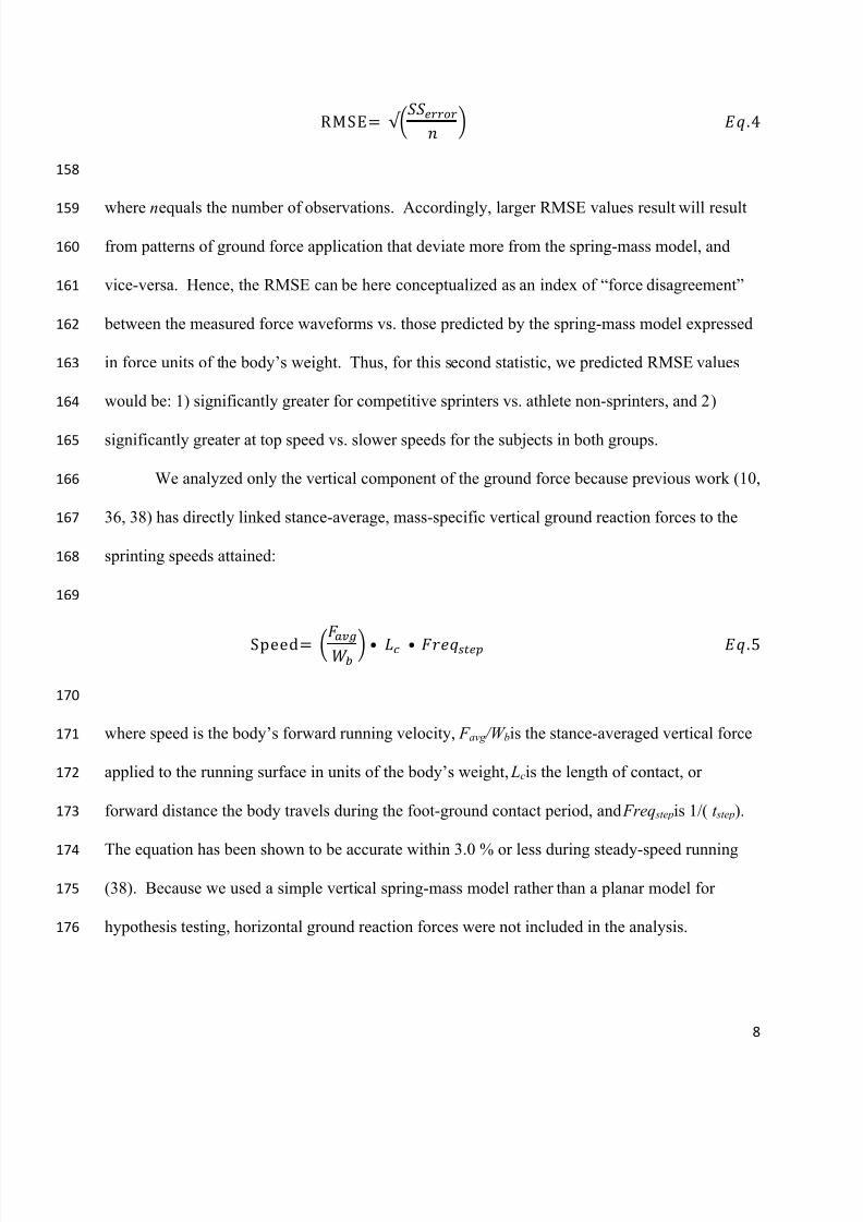
RMSE= √ .4

158

where n equals the number of observations. Accordingly, larger RMSE values result will result159

from patterns of ground force application that deviate more from the spring-mass model, and160

vice-versa. Hence, the RMSE can be here conceptualized as an index of “force disagreement”161

between the measured force waveforms vs. those predicted by the spring-mass model expressed162

in force units of the body’s weight. Thus, for this second statistic, we predicted RMSE values163

would be: 1) significantly greater for competitive sprinters vs. athlete non-sprinters, and 2)164

significantly greater at top speed vs. slower speeds for the subjects in both groups.165

We analyzed only the vertical component of the ground force because previous work (10,166

36, 38) has directly linked stance-average, mass-specific vertical ground reaction forces to the167

sprinting speeds attained:168

169

Speed= • • .5

170

where speed is the body’s forward running velocity, F avg /W b is the stance-averaged vertical force171

applied to the running surface in units of the body’s weight, Lc is the length of contact, or172

forward distance the body travels during the foot-ground contact period, and Freq step is 1/( t step).173

The equation has been shown to be accurate within 3.0 % or less during steady-speed running174

(38). Because we used a simple vertical spring-mass model rather than a planar model for175

hypothesis testing, horizontal ground reaction forces were not included in the analysis.176



9

Design and Data Acquisition Strategies: For the competitive sprinter group, we recruited only177

track athletes who specialized in the 100 and 200-meter events and who had intercollegiate track178

and field experience or the equivalent. For the athlete non-sprinter group, we recruited athletes179

who regularly ran at high speeds for their sport specialization, but who were not competitive180

sprinters. In both groups, we recruited and enrolled only those athletes with mid- and fore-foot181

strike patterns because the fast subjects we were seeking to enroll do not heel strike when182

running at high speeds.183

We maximized ground reaction force data quality and quantity by conducting tests on a184

high-speed force treadmill capable of acquiring a large number of consecutive footfalls at185

precisely controlled speeds. Acquiring equivalently robust data for the purpose of quantifying186

patterns of foot-ground force application using in-ground force plates would be difficult, or187

perhaps impossible, given that overground conditions greatly limit the number of footfalls188

acquired, and substantially increases the variability present in both running speeds and foot-189

strike patterns. For athletic subjects running on a treadmill versus overground, prior studies have190

demonstrated a close correspondence between sprint running performances (9), sprinting191

kinematics (20) and patterns of ground force application at speeds at which comparative data are192

available (22, 29).193

Although we acquired data from many speeds, we used the ground reaction force data194

from only three of these for hypothesis testing: 5 m•s-1

, 7 m•s-1

, and individual top speed.195

196

Subjects and Participation197

A total of fourteen subjects, eight men and six women, volunteered and provided written,198

informed consent in accordance with the requirements of the local Institutional Review Board.199



10

All subjects were between 19 and 31 years of age and regularly active at the time of the testing.200

The compositions of the competitive sprinter group (age = 23.9 ± 1.6 years, height = 1.72 ± 0.03201

m, mass = 73.8 ± 4.3 kg) and the athlete non-sprinter group (age = 21.7 ± 1.5 years, height =202

1.77 ± 0.03 m, mass = 75.8 ± 4.6 kg) were gender balanced; both included four males and three203

females. Subjects ranged in athletic experience from intercollegiate team-sport athletes to204

professional, world-class track athletes. In the athlete, non-sprinter group, all seven subjects had205

intercollegiate athletic experience. In the competitive sprinter group, six of the seven subjects206

had intercollegiate track and field experience, five had international experience, and four had207

participated in both the Olympics and Track and Field World Championships. Physical208

characteristics and athletic descriptions of all participants appear in Table 1. Also provided are209

the 100 and 200 m personal records of the competitive sprinters.210

211

Measurements212

Top Speed (m•s-1

): Participants were habituated to running on a custom, high-speed force213

treadmill during one or more familiarization sessions before undergoing top speed testing. For214

all trials, subjects were fastened into a safety harness attached to an overhead suspension that215

would support them above the treadmill belt in the event of a fall. The harness and ceiling216

suspension had sufficient slack to not impede the subjects’ natural running mechanics. A217

progressive, discontinuous treadmill protocol similar to Weyand et al. (36) was administered to218

determine each subject’s top speed. The protocol began at speeds of 2.5 or 3.0 m•s-1

and219

typically increased in 1.0 m•s-1

increments for each trial at slower speeds and 0.2-0.5 m•s-1

at220

faster speeds. Trial speeds were progressively increased until a speed was reached at which the221

subject could not complete eight consecutive steps without backward movement exceeding 0.2 m222



11

on the treadmill. Subjects typically made two to three unsuccessful attempts at the failure speed223

before the test was terminated. The top speed successfully completed was within 0.3 m•s-1

of the224

failure speed for all subjects. For each trial, subjects straddled the treadmill belt as it was225

increased to the desired trial speed. Handrails on the sides of the treadmill were set at waist-226

height and aided the subject in their transition onto the moving belt. Once the treadmill belt had227

increased to the selected speed, subjects transitioned onto the belt by taking several steps before228

releasing the handrails. Data acquisition was not initiated until the subject had released the rails.229

There was no limit on the number of handrail-assisted steps the subjects could complete during230

their transition onto the belt. Trials at speeds slower than 5 m•s

-1

typically lasted 10 to 20231

seconds while trials at speeds faster than 5 m•s-1

typically lasted less than 5 seconds. Subjects232

were instructed to take full recovery between trials. They typically took one to two minutes233

between slow and intermediate speed trials, and one to ten minutes between faster speeds trials.234

To reduce the risk of injury or muscle soreness, testing was terminated before top speed was235

attained if the subjects reported muscle or joint discomfort.236

237

Treadmill Force Data: Ground reaction force data was acquired at 1,000 Hz from a high-speed,238

three-axis, force treadmill (AMTI, Watertown, MA, USA). The treadmill uses a Baldor239

BSM100C-4ATSAA custom high speed servo motor and a Baldor SD23H2A22-E stock servo240

controller and is capable of speeds of over 20 meters per second. The custom embedded force241

plate has a length of 198 cm and a width of 68 cm and interfaces with an AMTI DigiAmp242

amplifier running NetForce software. The force data was post-filtered using a low-pass, fourth-243

order, zero-phase-shift Butterworth filter with a cutoff frequency of 25 Hz (39).244



12

Stride timing, length, and center of mass motion variables were determined as follows.245

For each footfall, contact times were determined from the time the vertical force signal exceeded246

a threshold of 40 N. Aerial times were determined from the time elapsing between the end of247

one period of foot-ground contact and the beginning of the next. Step times were determined248

from the time elapsing during consecutive foot-ground contact and aerial times. Step frequencies249

were determined from the inverse of step times. Limb repositioning, or swing times, were250

determined from the time a given foot was not in contact with the running surface between251

consecutive steps. Contact lengths were determined by multiplying the time of foot-ground252

contact by the speed of the trial. Trial speeds were determined from the average belt velocity253

over time. The vertical displacement of the COM during ground contact period was determined254

by double integration of the vertical force waveforms following the procedures of Cavagna (12).255

256

Force Data Acquired : Individual subjects completed from 12 to 20 treadmill trials during their257

top speed tests to failure. The number of consecutive footfalls from which force waveforms258

were acquired during these tests was generally greater for the slower, less demanding trials. For259

example, we typically acquired > 20 consecutive footfalls for slow and intermediate speeds, 10260

to 20 at moderately fast speeds, and eight to 12 during top-speed, and near top-speed trials.261

The number of footfalls acquired at the subset of three speeds used for formal statistical testing262

purposes reflect the general pattern of acquiring fewer footfalls at faster speeds. For the263

competitive sprint and athlete non-sprint subjects, the average number of footfalls acquired at the264

three hypothesis test speeds were as follows: 31 and 28 at 5.0 m•s-1

, 23 and 13 at 7.0 m•s-1

and 10265

and 9 at top speed, respectively. The number of force waveforms acquired from the three266



13

selected speeds used for statistical testing purposes was 797. The total number of footfalls267

acquired from all subjects at all speeds was > 3000.268

For illustrative purposes, ensemble-averaged waveforms were determined for individual269

subjects and the two subject groups at all of the trial speeds completed including the top sprinting270

speed. For individual subjects at each speed of interest, ensemble-averaged waveforms were271

generated by averaging the force from each millisecond of the stance period for all of the272

waveforms acquired. At those speeds completed by all seven subjects of the respective groups,273

the seven individual ensemble-averaged waveforms were combined to form ensemble-averages274

for each of the respective groups. These group force-time waveforms were compiled by275

standardizing the vertical force values to units of the body’s weight and time values to the276

percentage of the total stance contact time. Neither the individual nor group ensemble averages277

were used for formal hypothesis testing purposes.278

To provide a supplementary assessment of waveform shape characteristics, we also279

performed a basic Fourier analysis in the tradition of Alexander & Jayes (1) that appears in the280

Appendix.281

282

Statistics283

Both hypothesis tests were evaluated using a two-factor ANOVA (Group x Speed) that analyzed284

the mean goodness of fit (R 2 values) between spring-model predicted ground reaction force285

waveforms and those directly measured from our subjects. Secondary tests of the same286

hypotheses were conducted using the RMSE statistic. For both force application hypothesis test287

one (group effect) and test two (speed effect), the a priori thresholds for significance were set at288

the α = 0.05 level. Homogeneity of variance was tested using the Fligner-Killeen test.289



14

Percentage differences between group means for all variables were calculated as:290

[(Larger – Smaller)/((Larger + Smaller)/2)] x 100. For stance-averaged vertical forces, mean291

percentage differences were calculated after subtracting a baseline value equal to 1.0 W b for292

running at zero speed, or standing.293

294



15

Results295

Top Speeds and Stance-Averaged Vertical Forces296

Group means (± SE) for top speeds, stance-averaged vertical forces, contact times, aerial times,297

swing times and contact lengths at top speed appear in Table 2. The table includes the overall298

group means for the competitive sprinters and athlete non-sprinters as well as the within-group299

means for the males and females. For the overall means, the between-group differences in two300

variables: top speed (∆ = 1.64 m•s-1

) and stance-averaged vertical forces (∆ = 0.21 W b), when301

expressed on a percentage basis (top speed ∆ = 17.2%; stance-average vertical force ∆ = 19.2%),302

were nearly identical. The similar percentage differences in top speed and stance-averaged force303

means variables across the groups resulted from the lack of variation in mean contact lengths and304

step frequencies (eq. 5).305

When considered for the respective genders, between-group differences in top speeds and306

stance-averaged vertical forces were both slightly larger for the female vs. male subjects (top307

speed ∆ = 1.76 vs. 1.56 m•s-1

; stance-averaged vertical force ∆ = 0.27 vs. 0.17 W b). Because308

neither step frequencies nor stance-averaged vertical forces varied appreciably by gender, the top309

speed differences between male and female subjects resulted largely from differences in contact310

lengths. The latter were 10.8% shorter for the overall female vs. male mean (female vs. male311

∆Lc: sprinters = 13.6%, athlete non-sprinters = 8.0%).312

313

Patterns of Ground Force Application as a Function of Running Speed314

Ground force application data from the same two female subjects, one sprinter and one athlete315

non-sprinter appear in Figures 2 through 4 to allow the relationships between original force316

waveforms (Figure 2), stance-averaged vertical forces (Figure 3), and patterns of ground force317



16

application (Figure 4) to be fully illustrated. The step-by-step, ground reaction force waveforms318

from these athletes’ respective top-speed trials (Figure 2A and B, respectively) were greater in319

magnitude and briefer in duration for the competitive sprinter vs. the athlete non-sprinter.320

The mass-specific, stance-averaged vertical forces for both athletes (Figure 3, panels A321

and B) increased in a largely linear fashion with speed, from a jog of 3.0 m•s-1

through top speed,322

with values for the sprinter being 0.2 W b greater across common speeds. Ensemble-averaged323

patterns of ground force application for the respective athletes at the same trial speeds (Figure 4,324

panels A and B) illustrate that both athletes had relatively symmetrical waveforms at the slowest325

speed of 3.0 m•s

-1

. With increases in speed above 3.0 m•s

-1

, patterns of ground force application326

by the sprinter became progressively less symmetrical. The corresponding waveforms for the327

athlete non-sprinter were relatively symmetrical across all speeds, including her top sprinting328

speed.329

330

Patterns of Ground Force Application vs. the Spring-Mass Model331

Ensemble-averaged patterns of ground force application at 5.0 m•s-1 , 7.0 m•s -1 and top speed, as332

well as their quantitative relationship to the spring-mass model predicted waveforms, appear in333

Figure 5 for one male sprinter (panels A, C, E) and one male athlete non-sprinter (panels B, D,334

F). The male sprinter’s waveforms have a qualitatively biphasic appearance due the rapid rising335

edge and early force peaks present on the waveforms at all three speeds. Thus, patterns of336

ground force application for the sprinter were generally in relatively poor agreement with the337

spring-mass model at all three speeds (all R 2 values < 0.80). Because the rising edges of the338

waveforms were steeper, and the early force peaks were greater in magnitude at faster speeds,339

the degree of conformation of the sprinters waveforms to the spring-mass model decreased as340



17

speed increased, reaching an R 2 minimum of 0.67 at top speed. The ground reaction force341

waveforms of the male athlete non-sprinter lacked a rapid rising edge and conformed relatively342

closely to the spring-mass model at all three speeds (R 2

range: 0.93-0.94).343

The ensemble-averaged waveform patterns of ground force application for the344

competitive sprint group and athlete non-sprint groups at the three test speeds (Figure 6)345

exhibited the same patterns similar to those of the individual athletes in Figure 5, albeit to a346

slightly smaller degree. The rising edge of the group ensemble-averaged waveform for the347

competitive sprinters was steeper in general than that of the athlete non-sprinters, and became348

progressively more steep at the faster speeds. The group ensemble-averaged patterns of ground349

force application of the athlete, non-sprinters conformed closely to the spring-modeled350

waveforms at all three speeds (all R 2 values ≥ 0.93), exhibiting little discernible speed-related351

deviation.352

The relative stance times at which the peak force occurred during top speed running, as353

assessed from the group composite waver forms in Figures 6E and F, were t =30.2% of t c for354

competitive sprinters and t =45.7% of t c for the athlete non-sprinters. The corresponding values355

for the percentage of the total contact time at which the center of mass reached its minimum356

height, as determined from the double-integration of the composite, top speed waveforms in357

Figure 6 were t =40.5% of t c and t =48.7% of t c for the competitive sprinters and athlete non-358

sprinters, respectively.359

360

Hypothesis One and Two: Statistical Test Results361

The R 2 goodness of spring fit and RMSE force disagreement values (mean ± SE) from the362

footfall waveforms (n=797) analyzed at 5.0 m•s-1

, 7.0 m•s-1

and top speed appear in Table 3. In363



18

keeping with our first hypothesis, the patterns of ground force application of the competitive364

sprinters conformed significantly less to the spring-mass model predictions than those of athlete365

non-sprinters when evaluated with the R 2 goodness of fit statistic (two-factor ANOVA, F =366

243.8, p < 0.001). This was the case even when the much greater variability in the waveforms of367

the sprinters vs. athlete non-sprinters was taken into account by the Fligner-Killeen test. In368

partial support of our second hypothesis test using R 2 goodness of fit values, the patterns of369

ground force application conformed less to the simple spring-predicted pattern for sprinters at370

top speed than at 5.0 and 7.0 m•s-1

. However, there were no significant differences across speed371

for athlete non-sprinters whose goodness of fit values were nearly identical at 5.0 m•s

-1

, 7.0 m•s

-1

372

and top speed. Hence, interaction between athletic group and running speed was significant [F =373

51.5, p < 0.01].374

The hypothesis test results obtained when RMSE values were used to evaluate patterns of375

ground force application vs. those predicted by the spring-mass model were fully consistent with376

the results of the R 2 tests. The main effect of athletic group was significant and there was an377

interaction between group and running speed. After again accounting for the lack of378

homogeneity of variance as tested by the Fligner-Killeen test, the RMSE force disagreement379

values vs. the simple-spring patterns predicted by the spring-mass model at all three test speeds380

were significantly greater for the competitive sprinters than the athlete non-sprinters [F = 442.8;381

df = 1, 795; p < 0.001]. RMSE values were also statistically different across the three running382

speeds [F = 104.0; df = 5, 791; p < 0.001] with post-hoc testing indicating that this difference383

was present for the competitive sprinters, but not the athlete, non-sprinters (Table 3).384

385

386



19

Individual Variability in Patterns of Ground Force Application387

At each of the three analysis speeds, the standard errors about the R 2 and RMSE means were388

approximately two times greater for the sprinters than the athlete non-sprinters (Table 3). The389

greatest within-group stratification for both variables existed among the four males in the390

competitive sprinter group. For the ensemble-averaged waveforms, Subjects 1 and 2 had391

respective R 2 goodness of fit values to the spring-mass model predicted waveforms of 0.78 and392

0.73 across the three test speeds while subjects 3 and 4 had respective values of 0.89 and 0.91.393

The corresponding RMSE values for subjects 1 and 2 were 0.62 and 0.58 W b, respectively, vs.394

0.35 and 0.37 W b for subjects 3 and 4. Top speed patterns of ground force application for these395

respective pairs of competitive male sprinters (subjects 1 and 2, elite vs. subjects 3 and 4, sub-396

elite) and the corresponding ensemble average of all of the male subjects in the athlete non-397

sprinter group (n = 4) appear in Figure 7A. The trend most evident for male sprinters was398

present throughout the entire sample. Differences in the stance-average vertical forces applied at399

top speed were determined entirely during the first half of the stance period (Figure 7B) as all 14400

subjects in our sample applied nearly the same vertical force over the second half of the stance401

phase (1.72 ± 0.04 W b).402

403

404

405



20

Discussion406

Our first objective was to answer the basic question posed in our title: is running speed407

maximized with simple-spring, stance mechanics? Although selected results did not conform408

precisely to our predictions, our data in total provided a definitively negative answer. With409

nearly complete consistency, we found that the runners who applied the greatest mass-specific410

vertical forces, and thereby attained the fastest speeds, deviated most from the simple-spring411

pattern of ground force application predicted by the spring-mass model (Figures 2, 4, 5, 6 and 7,412

Table 3). Given the need for all runners to reduce periods of ground force application as they413

run faster, these data provide two closely linked conclusions. First, the simple-spring patterns of414

ground force application generally regarded as advantageous at slower speeds (15, 17) likely415

constrain force application and performance at faster ones. Second, deviating from simple-416

spring, stance mechanics appears to be a strategy that sprinters use (14) to apply the greater417

mass-specific ground forces needed to attain faster speeds.418

419

Hypothesis Test Outcomes: Simple-Spring Stance Mechanics at the Fastest Speeds?420

From a strictly experimental perspective, our first simple-spring hypothesis test outcome421

conformed to our expectations in full, while our second outcome conformed only in part. As422

predicted, test one, which used athletic specialization as an experimental tool, revealed that the423

patterns of ground force application of the competitive sprinters deviated more from simple-424

spring predicted behavior than those of athlete non-sprinters regardless of speed (Table 3).425

Between-group quantitative differences were sufficiently large to be qualitatively obvious from426

the shapes of the waveforms, whether for individual athletes (Figures 4 and 5), or the entire427

athletic specialty groups (Figures 6 and 7). However, test two, which used across-speed428



21

comparisons as an experimental tool, yielded results that were mixed by athletic specialization;429

differences across speed were present for the competitive sprinters, but absent for the athlete430

non-sprinters. For the competitive sprinters, R 2 pattern-agreement and RMSE force-431

disagreement values at 5.0 and 7.0 m•s-1

were similar to one another (R 2 range: 0.83 to 0.85;432

RMSE range: 0.43 to 0.44 W b, Table 3) while their top-speed patterns deviated significantly433

more from model predictions (R 2< 0.80; RMSE > 0.55 W b). Using our R

2 threshold of 0.90 for434

simple-spring vs. non-simple-spring patterns, the sprinters did not conform to simple-spring435

predictions at any of the three speeds, and deviated most at top speed. In contrast, the athlete436

non-sprinters used patterns of ground force application that conformed relatively closely (R

2

>437

0.90) regardless of whether they were running at top speed or the two fixed test speeds of 5.0 and438

7.0 m•s-1

(Table 3). Unlike the competitive sprinters, the athlete non-sprinters exhibited virtually439

no differences in their patterns of ground force application across speed. Both their R 2 pattern-440

agreement and RMSE force-disagreement values vs. the model predicted patterns model were441

essentially identical across 5.0 m•s-1

, 7.0 m•s-1

and top speed ( ∆R 2 < 0.02; ∆RMSE = 0.03 W b).442

Although our results across running speed were mixed with respect to our hypothesis, the443

conclusions regarding the force application patterns that maximize running speed were fully444

consistent. The across-speed results obtained from the competitive sprinters suggest that445

deviating from a simple-spring pattern of ground force application may be a mechanism these446

athletes used to attain faster speeds. Athlete non-sprinters, in contrast, did not alter their patterns447

across speed, nor deviate appreciably from simple-spring pattern at any speed. Notably, we448

found essentially the same pattern contrasts across individual subjects of differing performance449

capabilities. Of the four males in the competitive sprinter group, the two non-elite athletes450

(subjects 3 and 4) used top-speed, stance-limb mechanics reflective of their intermediate451



22

performance status. Specifically, these two sub-elite males had stance-limb mechanics that452

deviated more from the simple-spring predicted pattern than the athlete non-sprinters whom they453

could outperform. However, their mechanics deviated less from the pattern (R 2 means of 0.83454

vs. 0.71, respectively) than those of the two world-class males (Figure 7A, Table 3).455

Collectively, these observations suggest that the deviation from the simple-spring pattern456

observed for the world-class sprinters may be a force-augmentation mechanism that sub-elite457

sprinters cannot utilize to the same degree, and that athlete non-sprinters may be generally458

unable to use at all.459

460

The Applicability of the Spring-Mass Model to High-Speed Running 461

The broad acceptance of the spring-mass model over the course of the last two decades has been462

heavily based on running and hopping data from relatively slow speeds (4, 18, 19, 26, 33). The463

more recent application of the model to faster running speeds (25, 27, 34) is understandable464

given positive results from slower speeds and the limited data available at faster ones (6). The465

data set we have compiled here includes hundreds of high-speed running footfalls from athletes466

spanning a broad range of sprinting abilities. The emergent finding from these data that fastest467

speeds are achieved via consistent, specific deviation from the model’s predictions warrants468

critical evaluation of the spring-mass model’s assumed applicability to sprint running.469

One means of assessing relative conformation to the spring-mass model is examining the470

model-predicted force-motion dynamics vs. those actually observed. The model predicts that the471

peak force will occur at the temporal mid-point of the foot-ground contact period (i.e. at t =50%472

of t c), and that the center of mass will reach its lowest position at the same time. We found that473

our athlete non-sprinters conformed to these model predicted behaviors somewhat (Figure 6F),474



23

while our competitive sprint subjects conformed little or not at all. For the competitive sprinters475

at top speed, the group-averaged, ensemble waveform exhibited a force peak at t =30% of t c 476

(Figure 6E), and a corresponding height minimum of the center of mass at t =40% of t c rather477

than the model-predicted values of t =50% for both. Many of the individual sprinter’s waveforms478

at faster speeds had force peaks that occurred at t ≤25% of t c (Figures 2A, 4A, 5E) , and some479

exhibited two force peaks, with the first occurring at t ≈20% and the second at t ≈50% of t c 480

(Figure 5C). By even the most generous assessment, these results indicate that the spring-mass481

model is a poor descriptor of the stance-limb mechanics of high-caliber sprint athletes. These482

findings also raise basic questions about using the vertical and limb stiffness variables derived483

from the spring-mass model to describe the mechanics of running at higher speeds (25, 27, 34).484

The value of these stiffness variables as descriptors of sprint running mechanics is at best unclear485

if sprinting performance is optimized by not conforming to the assumptions required to calculate486

them.487

The prior success of the spring-mass model as a descriptor of running mechanics raises488

an immediate question regarding our negative test outcomes for sprinters: why do these athletes489

not conform to the model when so many other runners and hoppers do? Our results suggest that490

the performance demands of sprinting are probably not compatible with the stance-limb491

mechanics predicted by the simple, linear spring in the spring-mass model. The latter were492

formulated as a mechanical approximation for describing the apparently spring-like center of493

mass dynamics observed in the early, classic studies on gait mechanics (4, 11, 26). The presence494

of spring-like mechanics that the original investigators inferred at the level of the whole limb495

have subsequently been measured in selected muscles, tendons and ligaments that contribute to496

the limb’s overall behavior (21, 30). Indeed, during slower-speed running and hopping, the497



24

tissue-level stretch-shortening cycles (21, 31) that conserve mechanical energy could contribute498

as theorized to waveform patterns that generally conform to the predictions of the spring-mass499

model at these speeds (8). However, as considered in detail elsewhere (10), the success of500

sprinters does not depend upon either the conservation of mechanical energy or locomotor501

economy, but rather upon the ability to apply large mass-specific forces to the ground quickly.502

An important caution is warranted in the interpretation of our finding that the mechanics503

of the fastest human runners generally do not conform to the predictions of the spring-mass504

model. Specifically, the deviations we report from the simple, linear-spring predicted behavior505

of the model should not be interpreted more broadly as an absence of either spring-like dynamics506

or energy storage. Indeed, the greater ground reaction forces observed in faster runners and at507

faster speeds almost certainly coincide with relatively greater tissue strains and energy storage508

(21, 31). Rather, our findings are best understood within the context of our test objectives and509

the limitations of the classic spring-mass model. Our objectives required a null standard of510

comparison for the purpose of quantifying different patterns of ground force application. We511

used the simple, linear-spring predictions of the spring-mass model for this purpose because512

these waveforms have served as the literature standard for well over a decade. However, our513

objectives could have been just as easily met by using some other pattern as a standard of514

comparison. Accordingly, we caution against interpreting the patterns reported in a spring515

dynamics and energy storage framework.516

517

Ground Force Application Strategies for Speed518

Swifter runners are known to attain their faster top speeds primarily by applying greater mass-519

specific forces to the ground, but the mechanism by which they do so has not been previously520



25

identified. Here, two design strategies helped us to elucidate the force application strategy they521

use. First, we chose to analyze force application on a millisecond-by-millisecond basis rather522

than by averaging over the full stance period (per Figure 3) as previously (36-38). Second, we523

recruited a pool of athletic subjects with a fairly broad range of individual top speeds. The latter524

strategy included enrolling four sprinters who were world-class track athletes (Table 1, subjects525

1, 2, 5, 6) and a fifth who was a national-class athlete with Olympic and World Championship526

experience (subject 7). The scores of sprint-running force waveforms acquired from this527

heterogeneous group of fast-running athletes provided force and speed data not previously528

available from this population. The consistent manner in which faster runners deviated from the529

pattern predicted by the simple spring-mass model to apply greater mass-specific forces provided530

crucial mechanistic insight.531

Our finding that speed is maximized via a common force application strategy was532

certainly not a foregone conclusion at the outset of the study. From a purely theoretical533

perspective, the data acquired might have resulted in several outcomes other than the one we534

obtained. For example, faster athletes might have applied greater forces while utilizing a simple,535

linear-spring pattern. Alternatively, they might have employed an asymmetrical strategy that536

resulted in the greatest forces occurring later, rather than earlier, in the stance period. Finally,537

different athletes might have used different patterns to maximize force application and speed.538

Our finding that the degree of conformation to a particular pattern was consistently related to539

magnitude of the mass-specific force applied and top speeds attained provides two basic540

conclusions. First, our data indicate that the fastest human runners have converged on a common541

mechanical solution for maximizing ground force and speed. Second, the convergence on a542



26

common solution implies the existence of a single most effective mechanism by which human543

runners can maximize speed.544

Indeed, the mechanical strategy identified was so consistent that even simple approaches545

to examining stance-phase patterns of force application were sufficient to reveal it. When the top546

speed forces of our 14 subjects were assessed by dividing the stance period into halves (Figure547

7B), this simple analysis revealed that individual differences in the total stance-averaged forces548

were all but completely determined during only one of the two periods. Specifically, we found a549

strong positive relationship between top speed and the average force applied during the first half550

of the stance period, and essentially no relationship to the average force applied during the551

second half. These respective results are illustrated in Figure 7B, with the first-half, best-fit552

relationships being provided by sex to appropriately account for the leg and contact length553

differences (eq. 5, Table 2) that directly influence top speeds.554

An immediate question raised by our findings is why essentially all of the differences in555

stance-averaged forces at top speed are attributable to a relatively small portion of the total556

stance period. We cannot answer this question fully on the basis of force application data alone.557

However, the results illustrated in Figure 7 and those from our Fourier analysis (see Appendix)558

are consistent with the impact-phase, limb-deceleration mechanism we have recently described559

(14). This mechanism appears to explain how several of the gait features classically associated560

with competitive sprinters (24) translate into the greater mass-specific ground forces they apply.561

First, the knee elevation sprinters achieve late in the swing phase appears to contribute to early-562

stance ground force application by allowing greater limb velocities to be achieved prior to foot-563

ground impact (24). Second, the erect stance-phase posture sprinters adopt likely contributes to564

the stiffness required to decelerate the limb and body relatively quickly after the instant of foot-565



27

ground impact. The progressive, rising-edge deviation observed vs. the simple spring pattern, in566

relation to both top sprinting speeds (Figures 5, 6, and 7) and across different speeds in567

individual sprinters (Figures 2A, 5A, C, E, 6A, C, E and 7) is consistent with the impact-phase,568

limb deceleration differences that may present across these trials (14).569

570

Concluding Remarks – A Ground Force Signature for Speed571

We conclude that a relatively specific, asymmetrical pattern of force application maximizes the572

ground forces runners can apply during the brief contact periods that sprinting requires. The573

factors responsible for the pattern are not yet fully known, but result in the fastest sprinters574

applying substantially greater forces than non-sprinters during the early portion of the stance575

period. Consistent pattern asymmetry among the swiftest sprinters, and less pronounced pattern576

asymmetry among less-swift athletes lead us to conclude that: 1) the fastest athletes have577

converged on a common mechanical solution for speed, and 2) that less-swift athletes generally578

do not execute the pattern. On this basis, we suggest that the force-time pattern documented here579

for the most competitive sprinters in our sample (Figure 7A) constitutes a ground force580

application signature for maximizing human running speeds.581

582

583

584

585

586

587

588

589



28

Appendix590

Vertical ground reaction force waveforms during running are composed of high frequency591

components due to the acceleration of the lower limb during the impact phase, and low592

frequency components due to the acceleration of the rest of the body during the entire contact593

phase (14). Fourier analysis can be used to analyze these components.594

Any time-varying signal s(t) can be represented as a sum of sine waves (39, Equation 2.3,595

p. 28) and can be expressed as596

597

() = (2 ) ( 1)

598

where ao is the mean of the signal, and f n, an, and θ n are the frequency, amplitude, and phase599

angle of the nth

harmonic. The signal or waveform can be reproduced from these variables using600

N harmonics, with reproductive accuracy increasing as N increases.601

To serve as an example of performing the Fourier analysis, the measured force data and602

modeled half-sine waveforms from Figures 5E and 5F were analyzed using Equation A1. For603

both the Competitive Sprinter and the Athlete Non-Sprinter, the trial average contact time was604

0.102 seconds. The force data was measured on an instrumented force treadmill and filtered at605

25 Hz. Four harmonics ( N =4) were sufficient to accurately reproduce the original measured data606

and the modeled half-sine waveforms.607

Tables A1-A4 provide the terms for the variables described in Equation A1. The608

waveforms appearing in panels A and B of Figure A1 were generated from the terms listed in609

Tables A1 and A3. Low frequency components (green line) include terms n=0 and n=1 and high610



29

frequency components (red line) include terms n=2, n=3, n=4. The summation of all611

components (blue line) accurately reproduces the original measured data.612

The appearance of waveform differences above, but not below, the 10 Hz domain, is613

consistent with the time course of the impact-phase, force-enhancement mechanism proposed614

recently (14) and included here to explain the differences observed between the patterns of615

ground force of competitive sprinters vs. athlete, non-sprinters.616

617

618

619

620

621

622

623

624

625

626

627

628

629

630

631

632

633

634

635



30

Acknowledgments636

The authors would like to thank Dr. Laurence Ryan for assistance with the data collection,637

instrumentation, technical support, manuscript critiques, and substantial contributions to the638

scientific analysis, Dr. Kyle Roberts for his contributions to the statistical analysis, Coach639

Andreas Behm and Dr. Robert Chapman for strategic guidance and support, and the 14 athletes640

who made the study possible by volunteering their time and effort.641

642

Grants643

This work was partially supported by a US Army Medical and Materiel Command award644

(DAMD 17-02-2-0053) to PGW and funding from SMU’s Simmons School of Education and645

Human Development to KPC.646

647



31

References648

1. Alexander RM, Jayes AS. Fourier analysis of the forces exerted in walking and running. 649

J Biomech 13: 383-390, 1980. 650

2. Alexander RM, Maloiy GMO, Hunter B, Jayes AS, Nturibi J. Mechanical stresses651

during fast locomotion of buffalo (Syncerus caffer) and elephant (Loxodonta africana). J652

Zool Lond 189: 135-144, 1979.653

3. Bezodis IN, Kerwin DG, Salo AIT. Lower-limb mechanics during the support phase of654

maximum-velocity sprint running. Med Sci Sports Exerc 40: 707-715, 2008.655

4.

Blickhan R. The spring-mass model for running and hopping. J Biomech 22: 1217-1227,656

1989.657

5. Bruggeman GP, Arampatzis A, Emrich F, Potthast W. Biomechanics of double658

transtibial amputee sprinting using dedicated sprint prostheses. Sports Technol 1: 220– 659

227, 2009.660

6. Brughelli M, Cronin J. A review of the literature on the mechanical stiffness in running661

and jumping: methodology and implications. Scand J Sport Med 18: 417-426, 2008.662

7. Bullimore SR, Burn JF. Consequences of forward translation of the point of force663

application for the mechanics of running. J Theo Biol 238: 211-219, 2006.664

8. Bullimore SR, Burn JF. Ability of the planar spring–mass model to predict mechanical665

parameters in running humans. J Theo Biol 248: 686-695, 2007.666

9. Bundle MW, Hoyt RW, Weyand PG. High speed running performance: a new667

approach to assessment and prediction. J Appl Physiol 95: 1955–1962, 2003.668

10. Bundle MW, Weyand PG. Sprint Exercise Performance: Does Metabolic Power Matter?669

Exerc Sport Sci Rev 40: 174-182, 2012.670



32

11. Cavagna GA, Sabiene FP, Margaria R. Mechanical work in running. J Appl Phyisol 671

19: 249-256, 1964.672

12. Cavagna GA. Force platforms as ergometers. J Appl Physiol 39: 174-179, 1975.673

13. Cavagna GA, Heglund NC, Taylor CR. Two basic mechanisms for minimizing energy674

expenditure. American Journal of Physiology 233: R243-61, 1977.675

14. Clark KP, Ryan LJ, Weyand PG. Foot speed, foot-strike and footwear: linking gait676

mechanics and running ground reaction forces. J Exp Biol 217: 2037-2040, 2014.677

15. Dalleau G, Belli A, Bourdin M, Lacour JR. The spring-mass model and the energy678

cost of treadmill running. Eur J Appl Physiol 77: 257-263, 1998. 679

16. Dickinson MH, Farley CT, Full RJ, Koehl MA, Kram R, Lehman S. How animals680

move: an integrated view. Science, 288: 100-106, 2000.681

17. Farley CT, Blickhan R, Saiot J, Taylor CR. Hopping frequency in humans: a test of682

how springs set stride frequency in bouncing gaits. J Appl Physiol 71: 2127-2132, 1991.683

18. Farley CT, Gonzalez O. Leg stiffness and stride frequency in human running. J Biomech684

29: 181–186, 1996.685

19. Farley CT, Houdijk HHP, Van Strien C, Louie M. Mechanism of leg stiffness686

adjustment for hopping on surfaces of different stiffnesses. J Appl Physiol 85:1044-1055,687

1998.688

20. Frishberg BA. An analysis of overground and treadmill sprinting. Med Sci Sports Exerc689

15: 478–485, 1983.690

21. Ker RF, Bennett MB, Bibby SR, Kester RC, Alexander RM. The spring in the arch691

of the human foot. Nature 325: 147-149, 1987.692



34

33. Srinivasan M, Holmes P. How well can spring-mass-like telescoping leg models fit716

multi-pedal sagittal-plane locomotion data? J Theo Biol 255: 1-7, 2008.717

34. Taylor MJD, Beneke R. Spring-mass characteristics of the fastest men on earth. Int J718

Sport Med 33: 667-670, 2012.719

35. Usherwood JR, Hubel TY. Energetically optimal running requires torques about the720

centre of mass. J R Soc Interface 9: 2011-5, 2012.721

36. Weyand PG, Sternlight DB, Bellizzi MJ, Wright S. Faster top running speeds are722

achieved with greater ground forces not more rapid leg movements. J Appl Physiol 81:723

1991–1999, 2000.724

37. Weyand PG, Bundle MW, McGowan CP, Grabowski A, Brown MB, Kram R, Herr725

H. The fastest runner on artificial limbs: different limbs, similar function? J Appl Physiol726

107: 903-911, 2009.727

38. Weyand P, Sandell R, Prime D, Bundle M. The biological limits to running speed are728

imposed from the ground up. J Appl Physiol 108: 950-961, 2010.729

39.

Winter DA. Biomechanics and Motor Control of Human Movement. 2nd ed. NY: John730

Wiley and Sons, Inc., 1990.731

732

733



35

Figure Captions734

Figure 1. A schematic illustration of the classic spring-mass model (modified from Reference735

12) during forward running and the half-sine waveform representing the vertical force produced736

by the mathematical expression of the model (A). The half-sine waveform representing the737

spring-mass model (solid black line) vs. two different example waveforms. Example 1 (dashed738

black line) has low conformation to the model while Example 2 (dotted grey line) has greater739

conformation to the model (B). Ground reaction forces are presented in mass-specific form (i.e.740

after standardization to body weight) in all illustrations.741

Figure 2. Vertical ground reaction forces from four steps for a female competitive sprinter742

(panel A) and a female athlete non-sprinter (panel B) at their individual top speeds (10.3 and 8.1743

m•s-1

, respectively). The stance-averaged vertical forces applied during the respective trials are744

represented by the dashed horizontal lines. The competitive sprinter applies greater stance-745

averaged and peak vertical forces during briefer contact phases than the athlete non-sprinter.746

Figure 3. Stance-averaged, vertical force application across the range of running speeds for the747

same female competitive sprinter (squares) and female athlete non-sprinter (circles) whose data748

appear in Figure 2. For both subjects, stance-averaged vertical forces increased across the range749

of speeds. The competitive sprinter applied greater forces at equal speeds and top speed.750

Figure 4. Trial-averaged composite vertical ground reaction force waveforms across the range751

of running speeds for the same female competitive sprinter (panel A) and female athlete non-752

sprinter (panel B) whose data appeared in Figures 2-3. For both subjects, stance-averaged753

vertical forces increased and ground contact times decreased across the range of speeds.754

[Confidence intervals are omitted for clarity, here and in subsequent figures]. 755



36

Figure 5. The trial-averaged composite vertical ground reaction force waveform for a756

representative male competitive sprinter and representative male athlete non-sprinter are plotted757

against the half-sine waveform predicted by the spring-mass model for 5.0 m•s-1

, 7.0 m•s-1

, and758

each individual’s top speed (11.1 and 9.4 m•s-1

for the competitive sprinter and athlete non-759

sprinter, respectively). The stance mechanics of the competitive sprinter increasingly deviated760

from the spring model as the speeds increased from 5.0 m•s-1 to 7.0 m•s

-1 to top speed (panels761

A, C, and E), while the stance mechanics of the athlete non-sprinter generally conformed to the762

spring-mass model at all speeds (panels B, D, and F).763

Figure 6. The trial-averaged composite vertical ground reaction force waveform for the764

competitive sprinter group and the athlete non-sprinter group are plotted against the half-sine765

waveform predicted by the spring-mass model for 5.0 m•s-1

, 7.0 m•s-1

, and top speed. The stance766

mechanics of the competitive sprinters increasingly deviated from the spring-mass model as the767

speeds increased from 5.0 m•s-1to 7.0 m•s

-1 to top speed (panels A, C, and E), while the stance768

mechanics of the athlete non-sprinters generally conformed to the spring-mass model at all769

speeds (panels B, D, and F).770

Figure 7. Trial-averaged composite vertical ground reaction force waveforms at top speed for771

the two male elite sprinters (solid black line), the two male sub-elite sprinters (dotted black line),772

and four male athlete non-sprinters (solid grey line) (A). Average vertical forces for the first- and773

second-half of ground contact for subjects in both groups across the range of top speeds. Circles774

represent male subjects and triangles represent females subjects; open symbols represent average775

vertical forces for the first-half of ground contact while shaded symbols represent average776

vertical forces for the second-half of ground contact. Line fits for the data from the first-half of777

the ground contact period are provided by sex to appropriately account for the leg and contact778



37

length differences (eq. 5, Table 2) that influence top speeds. A single line fit for the data from the779

second-half of the ground contact period is plotted for all 14 subjects since the values are similar780

in magnitude across group and sex (B) [Linear best-fit regression equations appearing in B that781

relate ground force to top running speeds are as follows: Males 1st half stance, Force (W b) =782

0.26•Spd – 0.22; Females•1st half stance, Force (W b) = 0.23•Spd + 0.41, All subjects 2

nd half783

stance force, Force (W b) = 0.004•Spd + 1.68].784

785

Figure A1: Force vs. time waveforms as generated from the Fourier terms listed in Tables A1786

(Competitive Sprinter at 11.1 m•s

-1

, Panel A) and A3 (Athlete Non-Sprinter at 9.4 m•s

-1

, Panel787

B). Low frequency components (green line) include terms n=0 and n=1 and high frequency788

components (red line) include terms n =2, n =3, n =4. The summation of all components (blue789

line) accurately reproduces the original measured data.790



38

Table 1. Descriptive characteristics of the subjects.791

Group Gender Age Height (m) Mass (kg) Sport 100m PR (s) 200m PR (s)

Sprinter Male 28 1.85 91.6 Track and Field 9.96 20.57




Sprinter Female 23 1.70 61.8 Track and Field 11.12 22.29



Non-Sprinter Male 23 1.95 101.5 NCAA Varsity Football N/A N/A

Non-Sprinter Male 19 1.74 72.7 NCAA Club Lacrosse N/A N/A

Non-Sprinter Male 30 1.74 74.6 Former NCAA Varsity Soccer N/A N/A

Non-Sprinter Male 20 1.79 78.4 NCAA Distance Runner N/A N/A

Non-Sprinter Female 19 1.76 72.6 NCAA Varsity Soccer N/A N/A



792

793

794

795

796

797

798

799

800

801

802

803

804

805

806



39

Table 2. Top-speed gait mechanics.807

Group Top Speed (m•s-1) Favg (Wb) Lc (m) Tc (s) Taer (s) Tsw (s) Freqstep (s-1)

Sprinter

Males 10.84 ± 0.12 2.18 ± 0.02 1.10 ± 0.04 0.102 ± 0.004 0.114 ± 0.004 0.330 ± 0.010 4.65 ± 0.14

Females 9.73 ± 0.35 2.22 ± 0.06 0.96 ± 0.05 0.099 ± 0.002

0.118 ± 0.004

0.335 ± 0.006 4.61 ± 0.06

Average 10.36 ± 0.27 2.20 ± 0.03 1.04 ± 0.04 0.100 ± 0.002 0.116 ± 0.003 0.332 ± 0.006 4.63 ± 0.08

Non-Sprinter

Males 9.28 ± 0.17 2.01 ± 0.07 1.04 ± 0.06 0.112 ± 0.006 0.111 ± 0.006 0.334 ± 0.012 4.49 ± 0.14

Females 7.97 ± 0.19 1.95 ± 0.01 0.96 ± 0.02 0.121 ± 0.001 0.113 ± 0.005 0.346 ± 0.010 4.29 ± 0.10

Average 8.72 ± 0.29 1.99 ± 0.04 1.01 ± 0.03 0.116 ± 0.004 0.112 ± 0.004 0.340 ± 0.008 4.40 ± 0.09

Values are means ± SE.808

809

810

811

812

813

814

815

816

817

818

819

820

821

822

823

824



40

Table 3. Mean R2 Agreement and RMSE Force Disagreement values vs. the Spring-Mass Model825

Group No. of Steps R 2 RMSE (Wb)

Sprinters

5.0 m•s-1 218 0.829 ± 0.007 0.440 ± 0.009

7.0 m•s-1 163 0.843 ± 0.008 0.437 ± 0.012

Top Speed 67 0.782 ± 0.016* +

0.571 ± 0.025* +

Non-Sprinters

5.0 m•s-1 194 0.910 ± 0.003 0.276 ± 0.004

7.0 m•s-1 89 0.923 ± 0.004 0.276 ± 0.007

Top Speed 66 0.915 ± 0.006 0.307 ± 0.012

Values are means ± SE.826

Competitive sprinters differed significantly from athlete non-sprinters across all speeds for both R 2 pattern827

agreement and RMSE force disagreement values (ANOVA, main effects, p < 0.001).828

829

* Significantly different from 5.0 m•s-1830

+ Significantly different from 7.0 m•s-1

831

832

833

834

835

836

837

838

839

840

841

842

843

844



41

Table A1. Fourier Terms of Competitive Sprinter at 11.1 m•s-1 Measured Force Data845

n f n (Hz) an (Wb) θ n (radians)

0 - 2.1739 -

1 9.8039 1.5513 -0.9871

2 19.6078 0.6461 -1.2683

3 29.4118 -0.3049 0.66764 39.2157 -0.0678 0.0262

846

847

Table A2. Fourier Terms of Competitive Sprinter at 11.1 m•s-1 Modeled Half-Sine Waveform848


0 - 2.1739 -

1 9.8039 1.4664 -1.5721

2 19.6078 0.2968 -1.5733

3 29.4118 -0.1297 1.5672

4 39.2157 0.0740 -1.5755849

850

Table A3. Fourier Terms of Athlete Non-Sprinter at 9.4 m•s-1 Measured Force Data851


0 - 2.1199 -

1 9.8039 1.5324 -1.3331

2 19.6078 0.4448 -1.4240

3 29.4118 -0.1038 0.8629

4 39.2157 -0.0382 0.4151

852

853

Table A4. Fourier Terms of Athlete Non-Sprinter at 9.4 m•s-1 Modeled Half-Sine Waveform854


0 - 2.1199 -

1 9.8039 1.4299 -1.5721

2 19.6078 0.2895 -1.5733

3 29.4118 -0.1265 1.5672

4 39.2157 0.0722 -1.5755

855



2

2

Figure 1

V e r t i c a l F o r c e ( W

b )

Contact Time (%)

B

A



F o r c e ( W b )

Time s

Competitive Sprinter at 10.3 m•s-1 A

Stance-Averaged

Vertical Force

Athlete Non-Sprinter at 8.1 m•s-1 B

Stance-Averaged

Vertical Force

Figure 2



Figure 3

Body Weight



Figure 4

Contact Time (s)

V e r

t i c a l F o r c e ( W b )

Athlete Non-Sprinter

Competitive Sprinter

0

A

B



Figure 5

V e r t i c a l F o r c e ( W b )

Contact Time (s)

Competitive Sprinter

0

1

2

3

4

0 0.1 0.2

0

1

2

3

4

0

1

2

3

4

0 0.1 0.2

Athlete Non-Sprinter

R2 = 0.77RMSE (Wb) = 0.49

R2 = 0.93RMSE (Wb) = 0.25

R2 = 0.75RMSE (Wb) = 0.54

R2 = 0.94RMSE (Wb) = 0.26

R2 = 0.67RMSE (Wb) = 0.70

R2 = 0.93RMSE (Wb) = 0.30

5.0 m•s-1 5.0 m•s

-1

7.0 m•s-1 7.0 m•s

-1

9.4 m•s-1 11.1 m•s

-1

A B

C D

E F



0 25 50 75 100

0

1

2

3

4

0

1

2

3

4

0

1

2

3

4

0 25 50 75 100

Competitive SprinterGroup Average

5.0 m•s-1

5.0 m•s-1

7.0 m•s-1 7.0 m•s

-1

Top Speed Top Speed

R2 = 0.93

RMSE (Wb) = 0.25

R2 = 0.87

RMSE (Wb) = 0.42R

2 = 0.94

RMSE (Wb) = 0.24

R2 = 0.80

RMSE (Wb) = 0.56

R2 = 0.93

RMSE (Wb) = 0.29

V e r t i c a

l F o r c e ( W b )

Contact Time (%)

Athlete Non-SprinterGroup Average

R2 = 0.88

RMSE (Wb) = 0.39

Figure 6

A B

C D

E F



Figure 7

V e

r t i c a l F o r c e ( W b )

Contact Time (%)

A

V e r t i c a l F o r c e ( W b )

Top Speed (m•s-

)

B

First Half of

Ground Contact

Second Half of

Ground Contact



Figure A1.

strke mecanics stdy

Documents